phase light curves for extrasolar jupiters and saturnsulyana/ · phase light curves for extrasolar...

PHASE LIGHT CURVES FOR EXTRASOLAR JUPITERS AND SATURNS

Ulyana A. Dyudina,1, 2

Penny D. Sackett,2and Daniel D. R. Bayliss

3

Research School of Astronomy and Astrophysics, Mount Stromlo Observatory, Australian National University,

Cotter Road, Weston Creek, Canberra, ACT 2611, Australia

S. Seager

Observatories of the Carnegie Institution of Washington, 5241 Broad Branch Road NW, Washington, DC 20015

Carolyn C. Porco

CICLOPS, Space Science Institute, 3100 Marine Street, Suite A353, Boulder, CO 80303-1058

and

Henry B. Throop and Luke Dones

Southwest Research Institute, 1050 Walnut Street, Suite 426, Boulder, CO 80302

Received 2004 June 16; accepted 2004 September 16

ABSTRACT

We predict how a remote observer would see the brightness variations of giant planets similar to those in oursolar system as they orbit their central stars. Our models are the first to use measured anisotropic scatteringproperties of solar system giants and the first to consider the effects of eccentric orbits. We model the geometry ofJupiter, Saturn, and Saturn’s rings for varying orbital and viewing parameters, using scattering properties for the(forward scattering) planets and (backward scattering) rings as measured by the Pioneer and Voyager spacecraft at0.6–0.7 �m. Images of the planet with and without rings are simulated and used to calculate the disk-averagedluminosity varying along the orbit; that is, a light curve is generated. We find that the different scattering propertiesof Jupiter and Saturn (without rings) make a substantial difference in the shape of their light curves. Saturn-sizedrings increase the apparent luminosity of a planet by a factor of 2–3 for a wide range of geometries, an effect thatcould be confused with a larger planet size. Rings produce asymmetric light curves that are distinct from the lightcurve that the planet would have without rings, which could resolve this confusion. If radial velocity data areavailable for the planet, the effect of the ring on the light curve can be distinguished from effects due to orbitaleccentricity. Nonringed planets on eccentric orbits produce light curves with maxima shifted relative to the po-sition of the maximum phase of the planet. Given radial velocity data, the amount of the shift restricts the planet’sunknown orbital inclination and therefore its mass. A combination of radial velocity data and a light curve for anonringed planet on an eccentric orbit can also be used to constrain the surface scattering properties of the planetand thus describe the clouds covering the planet. We summarize our results for the detectability of exoplanets inreflected light in a chart of light-curve amplitudes of nonringed planets for different eccentricities, inclinations, andazimuthal viewing angles of the observer.

Subject headingg: methods: data analysis — planetary systems — planets: rings —planets and satellites: individual (Jupiter, Saturn) — scattering

1. INTRODUCTION

Modern space-based telescopes and instrumentation are nowapproaching the precision at which reflected light from extra-solar planets can be detected directly (Jenkins & Doyle 2003;Walker et al. 2003; Green et al. 2003; Hatzes 2003). Since1995,more than 100 extrasolar planets (or exoplanets) have been de-tected indirectly by measuring the reflex motion of their parentstar along the line of sight (radial velocity or Doppler method).One of these radial velocity planets, Gl876b, has been confirmedby measuring the parent star motion on the sky (astrometry;Benedict et al. 2002), and a second, HD 209458b, by measur-ing the change in parent star brightness as the planet executesa partial eclipse of its host (transit photometry; Charbonneauet al. 2000; Henry et al. 2000). Three exoplanets have now

been detected by transit photometry (Udalski et al. 2002a,2002b, 2003) and then confirmed with Doppler measure-ments (Konacki et al. 2003, 2004; Bouchy et al. 2004). It is ex-pected that in the next decade, as photometric techniques areimproved from both the ground and in space, detection of thereflected light from exoplanets will prove useful not only in ex-panding the number of known exoplanets but also in detailingtheir characteristics.4

Reflected light from an exoplanet can be detected in twoways. First, with precise, integrated photometry, one cansearch for temporal variations in the combined parent star andexoplanet light curve due to the planet changing phase in re-flected light throughout its orbit, in the same way as the Moonchanges phase. The vast majority of the light comes from thestar itself, with a small constant thermal contribution for giantplanets, but if the periodic variations due to light reflected bythe planets can be extracted from the total phase light curve, the1 NASA Goddard Institute for Space Studies, 2880 Broadway, New York,

NY 10025.2 Planetary Science Institute, Australian National University, ACT 0200,

Australia.3 Victoria University of Wellington, New Zealand.

4 Reviews and references on extrasolar planets and detection techniquescan be found at http://www.obspm.fr /encycl /encycl.html.

973

The Astrophysical Journal, 618:973–986, 2005 January 10

# 2005. The American Astronomical Society. All rights reserved. Printed in U.S.A.

planetary phase as a function of time can be deduced. Fur-thermore, since the planet’s light and the starlight need notbe spatially resolved, relatively distant planetary systems andplanets at small physical orbital radii can be studied.

Already, ground-based observations of known short-periodexoplanets have been conducted to search for reflected lightsignatures in high-resolution spectroscopy (Charbonneau et al.1999; Collier Cameron et al. 2002; Leigh et al. 2003a, 2003b).To date, no signature of reflected light has been detected, but be-cause the orbital phase is known from radial velocity measure-ments, these nondetections constrain the gray geometric albedop of the planet for an assumed phase curve, orbital inclination,and planetary radius. For the assumed parameters of � Boo b,HD 75289b, and the innermost planet of � And, nondetectionsseem to imply that p < 0:4 (Collier Cameron et al. 2002; Leighet al. 2003a, 2003b).

Second, with sufficient spatial resolution, direct imaging canresolve the planet and the star in space, so that the projectedplanetary orbit can be tracked simultaneously with the mea-surement of the planet’s phases in reflected light. To be de-tected, planets must be at orbital distances large enough to beeasily resolved from their parent star and yet close enough thatthe reflected brightness is large enough to be detected againstthe background. Consequently, the first extrasolar planets to bedetected directly in this way are likely to be giants orbiting rel-atively nearby stars (at tens of parsecs) at intermediate semi-major axes (1–5 AU; Clampin et al. 2001; Lardiere et al. 2004;Trauger et al. 2003; Krist et al. 2003; Codona & Angel 2004;Dekany et al. 2004).

Direct imaging can yield both the orbit and the luminosityof the planet simultaneously and thus yield robust detections.Although direct exoplanet imaging from either the ground orspace may not be available for several years, our model lightcurves can be used for planning future observations of spatiallyresolved planets in reflected light.

The potential of exoplanet detection in reflected light and thepossibility of detecting planetary rings is demonstrated by thenumber of works published in the last few years. Seager et al.(2000) modeled the atmospheric and cloud composition andsimulated the light curves for close-in giant planets with var-ious cloud coverages. Sudarsky et al. (2003) modeled cloudsand spectra for extrasolar planets at different distances from thestar. Barnes & Fortney (2004) modeled transit light curves for aplanet with rings. Arnold & Schneider (2004) simulated lightcurves for planets with rings of different sizes, assumingplanets with isotropically scattering (Lambertian) surfaces andrings with isotropically scattering particles, and provided adiscussion of the possibility of ring presence at different stagesof planetary system evolution.

Our model, however, is the first to use the observed aniso-tropic scattering of Jupiter, Saturn, and Saturn’s rings and thefirst to calculate light curves for eccentric orbits. We find thatanisotropic scattering yields light curves that are substantiallydifferent from those assuming Lambertian planets and iso-tropically scattering rings and thus is more likely to give anaccurate description for extrasolar planets similar to Jupiter andSaturn.

In x 2 we describe our model. In x 3 we present our lightcurves for nonringed exo-Saturn and exo-Jupiter planets onan edge-on circular orbit, for variously oriented oblate exo-Saturns and for a ringed planet (with Saturnian scattering prop-erties) at variously inclined circular orbits. In addition, we modela nonringed exo-Saturn, an exo-Jupiter, and a Lambertianplanet on eccentric orbits. In x 4 we discuss the uncertainties

of our model and the detectability of the light curves bymodern and future instruments. Conclusions are presented inx 5.

2. MODEL

We model the reflected brightness of an exo-Jupiter or exo-Saturn by tracing how light rays from the central star are re-flected by each position on the planet. We then produce images(maps with a resolution of 16–200 pixels across, depending onthe acceptable error level) of the planet and its rings for dif-ferent geometries. The light rays from the star illuminating theplanet are assumed to be parallel, consistent with both star andplanet being negligible in size compared with the star-planetdistance. The reflected rays collected by the observer are as-sumed to be parallel, consistent with a remote observer. Themodel includes reflection from the planet and rings and therings’ transmission and shadows but does not incorporatesecond-order effects such as ring shine on the planet or planetshine on the rings. We account for the planet’s oblateness insome of our simulations by using the 10% oblateness of Saturnas an example.The planetary reflected brightness in our model is derived

from the data as an average brightness integrated along theplanet’s spectrum, weighted by the wavelength-dependenttransmissivity of the Pioneer red filter, which is nonzero in therange 0.595–0.720 �m. Our notation matches that of mostobservational papers on Saturn and Jupiter. To compare ourresults with those from the models of Arnold & Schneider(2004), we list both our and their parameter names in Table 1.Figure 1 demonstrates the geometry of a ringed planet on a

circular orbit defined by the angles listed in Table 1. Besidesthe angles shown in Figure 1, which define the geometry of theplanet as a whole, the scattering brightness of each position onthe planet’s or ring’s surface depends on three angles: the phaseangle � , the incidence angle via its cosine �0, and the emissionangle via its cosine �, as defined by the surface scattering phasefunction P(�0, �, � ). We obtain P(�0, �, � ) for Jupiter, Saturn,and the rings from the data as described in the subsectionsbelow.

2.1. ReflectinggProperties of Jupiter, Saturn, and RinggsFigure 2 shows the scattering phase function for a given

geometry, used in our model to describe surfaces of Jupiter,Saturn, and its rings. The normalized brightness of a point onthe surface is plotted versus scattering phase angle � :

P(�0; �; � ) � I(�; �0; �)=(F�0); ð1Þ

where F�0 is the ‘‘ideal’’ reflected brightness of a white, iso-tropically scattering (Lambertian) surface, �0 is the cosine ofthe incidence angle measured from the local vertical, and F(� sr)is the solar flux at the planet’s orbital distance. In our notation,� ¼ 0

�indicates backscattering and � ¼ 180

�indicates for-

ward scattering. Note the logarithmic scale of the ordinate andthe large amplitudes of the phase functions. Lambertian scat-tering with reflectivity 0.82 (matching the observed Saturn’sfull-disk albedo at opposition) is shown as a horizontal solid linefor comparison. We also indicate, for the same ring opacity,albedo, and geometry, the ring phase function used by Arnold& Schneider (2004), which assumes isotropically scatteringparticles. Figure 2 shows reflected light only for the geometryin which the Sun is 2� above the horizon (�0 ¼ 0:035) and theobserver moves from the Sun’s location (� ¼ 0

�) across the

DYUDINA ET AL.974

Fig. 1.—Angles defining the geometry of a ringed planet on a circular orbit observed from a large distance. Dashed lines show the normal to the ring plane andthe line of intersection of the ecliptic with the ring plane. The observer’s azimuth relative to the rings, !r , is positive when the rings are tilted from the ecliptic towardthe observer, is negative when the rings are tilted from the ecliptic away from the observer, and changes from �90� to 90�. We do not consider other possible valuesof !r ¼ �(90� 180�) because these orientations produce light curves symmetric to those with !r ¼ �(0� 90�) !r ¼ �0�. For a nonringed planet, the geometry isfully determined by the inclination i and the orbital angle �(t). For a ringed planet, the geometry is fully determined by i, �(t), !r, and the obliquity �.

TABLE 1

Parameters Used in Modeling

This Work Arnold & Schneider (2004) Quantity

A, B .......................... CoeDfficients of the Backstorm law

AHG........................... CoeDfficient for Jovian phase function

a, a1.......................... Semimajor axis of the planet’s orbit (AU)

DP ............................. Planet-star distance (km)

E ............................... Eccentric anomaly (polar angle parameterization)

e................................ Eccentricity

F ............................... � Intensity of a white Lambertian surfacea (W m�2 sr�1)

g1, g2, f ...................... Parameters of Henyey-Greenstein function

I ................................ Lp, IR, IT , Lps, Lpr Intensity (or brightness, or radiance) of the surface (W m�2 sr�1)

i ................................ i Inclination of the orbit (0�: face-on; 90�: edge-on) (deg)LP.............................. Luminosity of the planet b in reflected light

L*.............................. Luminosity of the star b

M .............................. Mean anomaly (time parameterization)

p................................ Full-disk albedo,b LP=(�R2PF )

P(�0, �, � ) .............. Scattering phase function of the surface

R ............................... Star’s magnitude in R band

RP ............................. rp Equatorial radius of the planet ( km)

rpix ............................ Pixel size (km)

V ............................... Star’s magnitude in V band

� ............................... � Phase angle (deg)

�t............................... Temporal shift of light-curve maximum from pericenter (days)

� ................................ Planet’s obliquity (deg)

� .............................. ¼ ��90� Orbital angle (�180�: minimum phase; 0�: maximum phase) (deg)

�0, �......................... �0, � Cosines of the incidence and emission angle

! ............................... Argument of pericenter (90�: observed from pericenter, �90�: from apocenter) (deg)

!r .............................. Observer’s azimuth relative to the rings (deg)

a F(� sr) is the incident stellar flux at the planet’s orbital distance (which is also sometimes called F but has W m�2 units, unlike our intensity Fmeasured per unit solid angle).

b The ‘‘red’’ or ‘‘blue’’ optical properties are the convolution of the planet’s (or the ring’s or the solar) spectrum with the wavelength-dependenttransmissivity of the Pioneer filter (which is nonzero between 0.595 and 0.720 �m for the red filter and between 0.390 and 0.500 �m for the bluefilter).

zenith toward the point on the horizon opposite the Sun(� ¼ 178

�). We used different methods to obtain P(�0, �, � )

for Jupiter, Saturn, and the rings from Pioneer and Voyagerdata.

2.1.1. Jupiter

For Jupiter we fitted a simple four-parameter analyticalfunction (two-term Henyey-Greenstein function) to the pub-lished data,

P(�0; �; � ) � AHG f PHG(g1; � )þ (1� f )PHG(g2; � )½ � ð2Þ

(Tomasko et al. 1978; Tomasko & Doose 1984). The coeffi-cient AHG is fitted to match the amplitude of the observedphase function. The individual terms are Henyey-Greensteinfunctions representing forward- and backward-scattering lobes,respectively:

PHG(g; � ) � 1� g2

(1þ g2 þ 2g cos � )3=2; ð3Þ

where � is the phase angle, f 2½0; 1� is the fraction of theforward versus backward scattering, and g is g1 or g2; g12½0; 1�controls the sharpness of the forward-scattering lobe, whileg22½�1; 0� controls the sharpness of the backward-scatteringlobe.

Figure 3 shows our fit of the Henyey-Greenstein function tothe data points from the Pioneer 10 and 11 images (Tomaskoet al. 1978; Smith & Tomasko 1984). This fitted function alsoreproduces the full-disk albedos observed by Karkoschka (1994,1998) at the wavelengths corresponding to the red passband ofPioneer. Pioneer images taken with broadband blue (0.390–0.500 �m) and red (0.595–0.720 �m) filters show surface loca-tions on Jupiter with different properties. In particular, Tomaskoet al. (1978) and Smith & Tomasko (1984) have indicated twotypes of locations: the belts, usually seen as dark stripes onJupiter (Fig. 3, crosses), and the zones, usually seen as brightstripes on Jupiter (Fig. 3, plus signs). The relative calibration

between Pioneer 10 and Pioneer 11 data is not as well con-strained as the calibration within each data set. If we acceptthe calibrations given in Tomasko et al. (1978) for Pioneer 10and those given in Smith & Tomasko (1984) for Pioneer 11,our model curve better represents the observations in the redfilter (black data points) than in the blue. The Pioneer 11 bluedata at moderate � in Figure 3 seem to be systematically off-set from the Pioneer 10 points, which may be a result of rel-ative calibration error. Consequently, we do not model the bluewavelengths.In addition to Pioneer data, images of Jupiter from a variety

of angles were taken by Voyager,Galileo, andCassini, althoughwe are not aware of any other published data of the scatteringphase functions for the Jovian surface.5 Data for � > 150� donot exist because these directions would risk pointing space-craft cameras too close to the Sun. Our derived light curves arenot severely affected by our extrapolation for � > 150�, how-ever, since when the forward scattering is important, the ob-served crescent is small, and the reflected light phase curveundergoes its minimum.

2.1.2. Saturn

The scattering phase function and albedo of Saturn are rep-resented by the Backstorm law, which was used by Dones et al.(1993) to fit observations of Saturn’s scattering:

IF

¼ A�

��0

�þ �0

� �B; ð4Þ

where A and B are coefficients that depend on the phaseangle � . The coefficients are fitted by Dones et al. (1993) toPioneer 11 phase function tables, which were produced by themultiple-scattering model of Tomasko & Doose (1984). Weaveraged the coefficients published by Dones et al. (1993)separately for zones and belts through Pioneer’s blue andred filters. Table 2 gives the resulting coefficients; Figure 2displays the red filter curve only. Figure 4 demonstrates the

5 One of us, U. A. D., plans to work on obtaining the spectral phasefunctions from Cassini nine-filter visible images in the immediate future.

Fig. 2.—Our model scattering phase functions for a Lambertian surface,Saturn, Jupiter, and Saturn’s rings and the phase function for rings consistingof isotropically scattering particles used by Arnold & Schneider (2004). Thephase functions are plotted for a single sample geometry: �0 is fixed (the Sunis 2

�above the horizon), while the observer moves in the plane that includes

the Sun and the zenith. The wavelengths correspond to visible red light (0.6–0.7 �m).

Fig. 3.—Our fit of the Henyey-Greenstein function (solid line; g1 ¼0:8; g2 ¼ �0:38; f ¼ 0:9, and AHG ¼ 2) to the Pioneer 10 data (P10), pub-lished as Tables IIa and IIb of Tomasko et al. (1978), and to the Pioneer 11data (P11), published as Tables IIa and IIb of Smith & Tomasko (1984). Thedata represent belts (dark stripes) and zones (bright stripes) on Jupiter ob-served with the red (0.595–0.720 �m) and blue (0.390–0.500 �m) filters.

DYUDINA ET AL.976 Vol. 618

difference between the blue and red phase functions forSaturn. The values for the blue curve are 1.5–2 times smaller,indicating that Saturn is darker in blue wavelengths because ofhigher absorption by photochemical hazes.

2.1.3. Saturn’s Ringgs

The ring brightness in reflection (illuminated side) andtransmission (unilluminated side) is provided by a physicalscattering model of the ring. This model calculates multiplescattering within the rings using a ray-tracing code. The modelring is populated with macroscopic bodies of size 1 m, withoptical depth and albedo profiles chosen to match those ofDones et al. (1993). The model reproduces well the bright-nesses observed by Voyager 1 and 2. We use the code to predictring brightness at geometries not observed by Voyager, bin theoutput into a look-up table, and then use the table to producethe ring images.

The ring brightness at each point is a function of threeangles (� , �, and �0), the optical depth, and the albedo. Becauseof data volume restrictions, we have binned output in ratherlarge steps, which depend on parameter values. These steps areclearly seen in the ring phase function in Figure 2 (dotted line).

2.2. Full-Disk AlbedoTo produce light curves of the fiducial exoplanets that we

model, images of the planet for a set of locations along the orbitare generated. For each image, we integrate the total light

coming from the planet and the rings (if any) to obtain the full-disk (or geometric) albedo p(� ):

p(� ) ¼P

pix I(�; �0; � )r 2pix=F�R2

P; ð5Þ

where rpix is the pixel size and RP is the planet’s radius. Thefull-disk albedo is the planet’s luminosity LP normalized bythe reflected luminosity of a Lambertian disk with the planet’sradius at the planet’s orbital distance, illuminated and ob-served from the normal direction:

p � LP=(�R2P F ): ð6Þ

2.3. Eccentric OrbitsIn addition to modeling light curves from ringed planets

traveling in circular orbits, we also model light curves ofnonringed planets moving in eccentric orbits. Although mostof the planets in the solar system orbit the Sun with low ec-centricities, the extrasolar planets detected to date display awide range of eccentricities.6 As can be seen in Figure 5, thegeometry of an ellipse introduces an additional parameter, inaddition to inclination, in the observer’s azimuthal perspectiveof the system. This parameter is the argument of pericenter, !,which is the angle (in the planet’s orbital plane) between theascending node line7 and pericenter (Murray & Dermott 2001).

To model the reflected light as a function of time, we cal-culate the angular position of the planet and the planet-starseparation over a complete period using a solution to Kepler’sequation: M ¼ E � e sin E, where M is the mean anomaly (aparameterization of time), E is the eccentric anomaly (a param-eterization of the polar angle), and e is the eccentricity. Kepler’sequation is transcendental and cannot be solved directly. Ap-plying the Newton-Ralphson method8 to Kepler’s equation, weobtain the iterative solution for the planet’s position:

Ei þ1 ¼ Ei � Ei � e sin Ei � Mi

1� e cos Ei: ð7Þ

3. RESULTS

The shape of the phase light curve depends on many pa-rameters: the planet’s orbit, its geometry relative to the ob-server, the planet’s oblateness, the scattering properties of the

TABLE 2

Coefficients for the Backstorm Function for Saturn

Phase Angle � 0� 30� 60� 90� 120� 150� 180�a

A (red, 0.64 �m).................... 1.69 1.59 1.45 1.34 1.37 2.23 3.09

B (red, 0.64 �m).................... 1.48 1.48 1.46 1.42 1.36 1.34 1.31

A (blue, 0.44 �m) ................. 0.63 0.59 0.56 0.56 1.69 1.86 3.03

B (blue, 0.44 �m) ................. 1.11 1.11 1.15 1.18 1.20 1.41 1.63

Note.—Coefficients for the Backstorm function for Saturn are averaged between belt and zone valuespublished in Table V of Dones et al. (1993).

a The coefficients at � ¼ 180� are not constrained by observations and were estimated by linearlyextrapolating the coefficients at 120� and 150�.

Fig. 4.—Scattering phase functions for Saturn in the red (0.595–0.720 �m)and blue (0.390–0.500 �m) passbands adopted from Dones et al. (1993) forthe same scattering geometry as in Fig. 2. The optical depth at the samplepoint on the rings (1.7 times Saturn’s radii from the planet’s center) is 2.3; thealbedo of the ring particles is 0.56. The ring is observed from the illuminatedside.

6 Eccentricities of extrasolar planets are listed at http://exoplanets.org /almanacframe.html.

7 The reference plane is formed by the observer’s line of sight and itsnormal in the ecliptic plane, which is also the ascending node line.

8 The application of the Newton-Ralphson method to Kepler’s equation isdescribed in Murray & Dermott (2001).

LIGHT CURVES FOR EXTRASOLAR PLANETS 977No. 2, 2005

planet’s surface, and the presence and geometry of rings. Tostudy whether these signatures can be identified unambiguouslyin the light curve, we modeled several geometries for the plan-etary system, i.e., different orbital eccentricities e for nonringedplanets and different ring obliquities � relative to the ecliptic forringed planets on circular orbits. For each of these cases, wemodeled a variety of observer locations, i.e., different orbital in-clinations i as seen by the observer and different azimuths !of the observer relative to the orbit’s pericenter or to the rings(!r). In what follows, we compare light curves for these differ-ing geometries and discuss whether or not different geometriceffects can be distinguished from one another.

3.1. Ligght Curvves for Jupiter vversus a Ringgless SaturnWe first compare spherical ringless exoplanets with different

surface reflection characteristics on circular orbits. Figure 6compares edge-on light curves for a ringless Saturn, a Jupiter,and a Lambertian planet. The reflected planet luminosity isnormalized by the incident stellar illumination to obtain thefull-disk albedo p as described in equations (5) and (6). Themodel planets have identical radii; the curves differ only be-cause of the different surface scattering of the three planets.

The full-disk albedo can be converted to the planet’s lumi-nosity LP as a fraction of the star’s luminosity L�*for a planet ofequatorial radius RP at an orbital distance DP,

LP=L� ¼ (RP=DP)2p: ð8Þ

For example, for Saturn at 1 AU, RP=DPð Þ2�1:6 ; 10�7. Theabscissa of Figure 6 indicates the azimuthal angle of the planetin its orbital plane (the orbital angle � of Fig. 1), starting atminimum planet phase (� ¼ �180�). The plot can be trans-formed into a time-dependent light curve simply by dividing� by 360

�and multiplying by the planet’s orbital period.

The light curve for Jupiter peaks much more sharply atfull phase (� � 0�) than the light curves of Saturn or the

Lambertian planet because of the sharp backscattering peak inJupiter’s scattering phase function (at � � 0� in Fig. 2). Nearzero phase (� � �180�) in Figure 6, Jupiter is more luminousthan the other two models because of the large forward scat-tering from its surface (� � 180�) in Figure 2. Such differ-ences in phase functions are commonly attributed to largerparticle size in the main cloud deck on Jupiter. For example,Tomasko et al. (1978) suggest particle sizes larger than 0.6 �mto explain the forward scattering.

3.2. Ligght Curvve for Oblate Planets vversus Spherical PlanetsNext we examine the effect of planet oblateness. Saturn’s

equatorial radius is 10% larger than its polar radius. This ob-lateness of Saturn (6% for Jupiter) makes the planet appearlarger when looking at the pole than when looking at the

Fig. 6.—Comparison of light curves for a spherical Jupiter, a sphericalSaturn, and a spherical Lambertian (isotropically scattering) planet, assumingthe planets are ringless and have the same radii RP. The planets differ onlyin their surface scattering properties. Albedos are shown for visible red light(0.6–0.7 �m).

Fig. 5.—Argument of pericenter, !, an additional angle needed to define the geometry of a nonringed planet on an eccentric orbit.


equator, which affects the light curves. Figure 7 compares lightcurves for a spherical planet, a 10% oblate planet viewed at itsequator, and a 10% oblate planet viewed at 45� latitude.

All three sample planets have the same equatorial radius andscattering properties as Saturn. We display light curves for anedge-on orbit (i ¼ 90�) of a planet rotating ‘‘on its side’’(� ¼ 90�), because this geometry emphasizes the effects ofoblateness in the reflected light. The differences among thecurves are created by differences in the observer’s azimuthrelative to the planet’s equator, an angle analogous to !r butmeasured with respect to the equatorial plane rather than thering plane. Observing the planet at the equator decreases thecross section of the planet and thus decreases the amplitude ofthe curve. Observing the planet at the pole yields a curve in-distinguishable from the solid curve for a spherical planet; this

is not shown in Figure 7. Observing the planet at 45� latitudeproduces a small asymmetry in the curve.

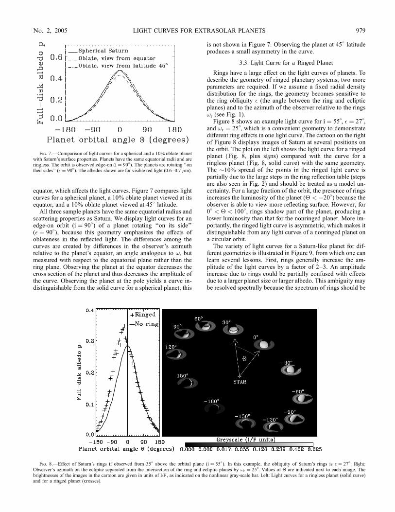
3.3. Ligght Curvve for a Ringged PlanetRings have a large effect on the light curves of planets. To

describe the geometry of ringed planetary systems, two moreparameters are required. If we assume a fixed radial densitydistribution for the rings, the geometry becomes sensitive tothe ring obliquity � (the angle between the ring and eclipticplanes) and to the azimuth of the observer relative to the rings!r (see Fig. 1).

Figure 8 shows an example light curve for i ¼ 55�, � ¼ 27�,and !r ¼ 25

�, which is a convenient geometry to demonstrate

different ring effects in one light curve. The cartoon on the rightof Figure 8 displays images of Saturn at several positions onthe orbit. The plot on the left shows the light curve for a ringedplanet (Fig. 8, plus signs) compared with the curve for aringless planet (Fig. 8, solid curve) with the same geometry.The �10% spread of the points in the ringed light curve ispartially due to the large steps in the ring reflection table (stepsare also seen in Fig. 2) and should be treated as a model un-certainty. For a large fraction of the orbit, the presence of ringsincreases the luminosity of the planet (� < �20

�) because the

observer is able to view more reflecting surface. However, for0� < � < 100�, rings shadow part of the planet, producing alower luminosity than that for the nonringed planet. More im-portantly, the ringed light curve is asymmetric, which makes itdistinguishable from any light curves of a nonringed planet ona circular orbit.

The variety of light curves for a Saturn-like planet for dif-ferent geometries is illustrated in Figure 9, from which one canlearn several lessons. First, rings generally increase the am-plitude of the light curves by a factor of 2–3. An amplitudeincrease due to rings could be partially confused with effectsdue to a larger planet size or larger albedo. This ambiguity maybe resolved spectrally because the spectrum of rings should be

Fig. 7.—Comparison of light curves for a spherical and a 10% oblate planetwith Saturn’s surface properties. Planets have the same equatorial radii and areringless. The orbit is observed edge-on (i ¼ 90�). The planets are rotating ‘‘ontheir sides’’ (� ¼ 90�). The albedos shown are for visible red light (0.6–0.7 �m).

Fig. 8.—Effect of Saturn’s rings if observed from 35� above the orbital plane (i ¼ 55�). In this example, the obliquity of Saturn’s rings is � ¼ 27�. Right:Observer’s azimuth on the ecliptic separated from the intersection of the ring and ecliptic planes by !r ¼ 25

�. Values of � are indicated next to each image. The

brightnesses of the images in the cartoon are given in units of I/F, as indicated on the nonlinear gray-scale bar. Left: Light curves for a ringless planet (solid curve)and for a ringed planet (crosses).


rather flat, whereas the planetary atmosphere is expected to bedark at a set of prominent gaseous absorption bands.

The second lesson is that light curves for a ringed planet areasymmetric. There are two types of asymmetry. The first, whichis potentially easier to detect, is the offset of the curve’s maxi-mum relative to � ¼ 0�, the maximum of the light curves for aringless planet (Fig. 9, vertical lines). The offset of the maxi-

mum itself occurs in a rather small fraction of the plots. How-ever, since the entire curve is asymmetric, the effect would bedetectable as an overall deviation from the simple symmetriccurves likely to be used to fit the first detections of reflected light.If radial velocity data exist for a planet, the exact timing of the� ¼ 0� point would be measurable. In this case, a shifted maxi-mum in the light curve would yield direct evidence of the rings.

Fig. 9.—Light curves for Saturn for different geometries. Different ring obliquities � are shown on each subplot as black curves of different line type. A curve for aspherical planet without rings is shown in gray. Each column corresponds to a different orbital inclination i. Each row corresponds to a different azimuth !r of theobserver relative to the rings.


The shifted maximum is a strong photometric signature thatwas also noted in the ring simulation of Arnold & Schneider(2004) as a ‘‘-shift.’’ We stress, however, that other processesmay be capable of producing such a -shift. Similar, althoughprobably smaller, shifts may be induced by a seasonal bright-ness variation on the planet. Note, however, that none of thegiant planets in the solar system have pronounced seasonalbrightness variations. The -shifts could also be produced by aglobal asymmetry of the brightness distribution over the planetor by the planet’s oblateness (see x 3.2). Again, spectroscopymay help to resolve the ambiguity between asymmetries causedby rings and those caused by processes on the planet surface.Abrupt asymmetric changes in the fine structure of the lightcurve give a more robust indication of the rings than a -shift,but resolving such detail would require another order of mag-nitude in instrument sensitivity.

The third lesson that we can draw from Figure 9 is that in thecase of face-on orbits (right column), both radial velocity ob-servations and precise photometry would give no signal for anonringed planet. A ringed planet, on the other hand, typicallyproduces a double brightness maximum, as the rings are illu-minated first from the observer’s side and then from the backside during the orbit (dotted curve). Double maxima can alsobe produced in eccentric orbits, but these have different finestructure (see x 3.4). We note, however, that a double peak maybe generated by seasonal variations or by an uneven brightnessdistribution at the planet’s surface.

3.4. Ligght Curvve for a Planet on an Eccentric OrbitAs an example of the effect orbital eccentricity may have on

the light curve of a planet in reflected light, Figure 10 showslight curves for a ringless planet with the orbital characteristicsof exoplanet HD 108147b and the equatorial radius of Jupiter.HD 108147b provides an interesting test case because someof the very first planets to be detected in reflected light will be‘‘close-in’’ and yet on eccentric orbits (HD 108147b has e ¼0:498 even though its semimajor axis is small at a ¼ 0:104 AU).We compare Lambertian, Jovian, and Saturnian scattering prop-erties in Figure 10 (top) to demonstrate the effect of anisotropicscattering, but the primary motivation for Figure 10 is to showthe effect of orbital eccentricity.9 The orbital parameters as-sumed for Figure 10 are those determined for HD 108147b byprecise radial velocity measurements (Pepe et al. 2002). Weassume the planet to be 10% oblate, as is Saturn. We plot thelight curve over one complete orbit, beginning at pericenter.

The light curves of Figure 10 can be rescaled easily for aplanet with the same orbital eccentricity but different semimajoraxis a1 by multiplying the luminosity by (a=a1)2 and multi-plying the time axis by the ratio of the orbital periods (a1=a)3=2.Since the inclination of the orbital plane cannot be determinedfrom radial velocity measurements, we display in Figure 10(bottom) light curves for inclinations between i ¼ 90

�(edge-

on) and 0�(face-on). Here we use Jovian scattering as our test

case because it produces the most prominent inclination fea-tures in the light curves. The argument of pericenter ! (seeFig. 5) can be derived from radial velocity measurements. ForHD 108147b, ! ¼ �41�, which means that we are fortunateto be at the azimuth at which the fullest planet phase � ¼ 0�

(Fig. 10, vertical line) is separated from pericenter by only

41�. With such a geometry, the phase-induced and eccentricity-induced maxima on the light curve amplify one another. As aresult, the amplitude of the curve for the edge-on case is about3:5 ; 10�5, nearly 5 times larger than for the face-on case, inwhich only the orbital distance variation matters.

Figure 11 illustrates the importance of the argument ofpericenter in determining the light curves of a given systemmeasured by the observer. The light curves assume the sameorbit as in Figure 10, but the argument of pericenter is now setto ! ¼ 60� rather than �41�. Such a change in the observer’sposition causes a threefold decrease in the amplitude of theedge-on (i ¼ 89

�) light curves.

For the ! ¼ 60� geometry, a secondary peak located close topericenter appears on the edge-on Jovian light curve. If the planetis less forward scattering than Jupiter (e.g., Saturn or a Lambertianplanet), the second peak does not appear. The i ¼ 89� and 75�

light curves display a sharp trough in which the amplitude of re-flected light is reduced almost to zero. This trough is due to theplanet showing no phase (‘‘newmoon’’) at this point of its orbit.

3.4.1. Temporal Shift of Ligght-Curvve Maximum �t

The position of the light-curve maximum relative to the peri-center (the temporal shift, �t, in Fig. 11) can yield important

Fig. 10.—Light curves for a planet on an eccentric orbit (orbital character-istics of exoplanet HD 108147b: a ¼ 0:104 AU, e ¼ 0:498), assuming Jupiter’sequatorial radius and 10% oblateness. The planet’s luminosity LP is normalizedby the star’s luminosity L

*and plotted vs. time. The argument of pericenter is

! ¼ �41�. The corresponding time of the planet’s maximum phase � ¼ 0�

(vertical line) is �0.4 days after pericenter (which defines time zero). Top:Comparison of edge-on light curves for planets with Jovian, Saturnian, andLambertian surfaces. Bottom: Comparison of different orbital inclinations fromface-on to edge-on orientations (i ¼ 1�–89�, respectively).

9 We do not expect a close-in planet such as HD 108147b to have cloudssimilar to those of Jupiter or Saturn, and we do not attempt to model in detailthe scattering properties of close-in planets. Our scattering models are moreappropriate for planets covered by water or ammonia clouds.


constraints on the inclination of the orbit and the cloud coverof the planet. First, as the inclination increases, the maximummoves from pericenter toward the time of the maximum phase� ¼ 0

�; i.e., �t increases. Unlike the amplitude of the curve,

which is also an indicator of inclination, �t cannot be producedby altering the planet’s size or albedo. However, this inter-pretation can be confused by the unknown strength of back-scattering at the planet’s ‘‘surface’’ (see Fig. 11, top).

Figure 12 summarizes the sensitivity of �t to the inclinationof the orbit and different atmospheric scattering properties.If radial velocity data exist for the planet, then the orbital ec-centricity e and argument of pericenter ! are known, and theshift, indicated by color coding in Figure 12, is observable. Theorbital inclination i (Fig. 12, ordinate) is generally not known,unless transit or astrometric data are available.

Our method of constraining the orbital inclination i usingFigure 12 is achieved by matching the measured �t values withthose along the vertical line corresponding to the known !on the plot with the appropriate eccentricity e, as measured byradial velocity techniques. An ambiguity remains because ofthe unknown scattering properties of the planet’s surface, whichcan sometimes be resolved by comparing the detailed shape ofthe light curves.

Second, �t may also serve to constrain the surface propertiesof the planet. In some cases, a lower limit may be put on thestrength of backscattering from the planet’s surface. For anyscattering surface, the maximum possible �t occurs on theedge-on orbit (i ¼ 90�); see examples in Figure 11 (top). Thelargest �t values are possible only from a strongly backscat-

tering planet. For example, in Figure 11, a 2 day �t can beproduced only by the Jovian planet.To learn whether the observed �t is high enough to restrict

atmospheric scattering, one can examine the three columns ofFigure 12, which summarize scattering from Jovian (left col-umn), Saturnian (middle column), and Lambertian planets (rightcolumn). As an example, if e ¼ 0:4, ! ¼ 60�, and the observedtemporal shift is 25% of the orbital period (green; �t values),only the left column, corresponding to Jovian scattering, dis-plays green anywhere along the! ¼ 60� vertical line; thus, onlystrongly backscattering planets like Jupiter could be consistentwith such an observation. Note, however, that this restrictionon atmospheric scattering may be contaminated by ring effects,large-scale bright patches on the planet’s surface, or seasonalvariation of the cloud coverage.

3.4.2. Contrast: Amplitude of Ligght-Curvve Variations

The contrast, or difference between the maximum and min-imum amplitude of the light curve, gives a measure of thedegree of variability that the planet’s reflected light displays. Itis this variation that new-generation space- or ground-basedphotometers may be able to detect if they can achieve the re-quired levels of precision.We plot the light-curve contrast for all possible orbital ori-

entations in Figure 13. These contour maps display the degreeof contrast for various orbital inclinations and arguments ofpericenter at given eccentricities. Note that the backscatter-ing peak of Jupiter’s surface makes the planet much darker atlow orbital inclinations than a Saturnian or Lambertian planet.For a given orientation, the more eccentric orbits show muchhigher contrast than do the circular orbits, although the amountof contrast depends strongly on both the inclination and theargument of pericenter. At high eccentricities, favorable ge-ometries (such as i ¼ 90� and ! ¼ �90) can increase thecontrast by approximately 5 times over those of less favorableorientations.

4. DISCUSSION

4.1. UncertaintiesOur model provides a rather accurate description of reflected

light curves for Jupiter and Saturn. The largest uncertainties aredue to the lack of observations at large phase angles (forwardscattering at � > 150

�) for the surfaces of Jupiter, Saturn, and

its rings. The extrapolations we have made to the phasefunctions could result in a factor of a few error in the brightnessat these angles, at which the light curves have their minimum.The contrast in the highest amplitude light curves (edge-onorbits) is constrained to within a few percent by high spectralresolution, ground-based observations of Saturn and Jupiter. Inour study, the uncertainty of these maximum amplitudes is10%–20% because the brightness of a planet varies with wave-length by about this amount within the 0.6–0.7 �m spectralrange (Karkoschka 1998).Reflectivity of the rings may be in error by as much as 50%

because many geometries, especially those for face-on ringillumination and face-on ring observation, are not constrainedby observations. New observations by the Cassini spacecraftwill fill this gap in the data. Another source of ring error is thescattering properties of the coarse grid in the tabulated ring (seex 2.1.3). This grid-induced noise is usually below 30% of thering’s luminosity.Rings around close-in, short-period exoplanets may be un-

likely because of tidal disruption and in any case can consist

Fig. 11.—Light curves for the same eccentric orbit as in Fig. 10, except thatthe argument of pericenter is ! ¼ 60�. The temporal shift �t is marked for theJovian nearly edge-on (i ¼ 89�) light curve.


only of rock. (Saturn’s rings are 99% ice.) Ice rings are stableagainst evaporation outside�7 AU for solar-type stars (Mekler& Podolak 1994). Rocky rings may be several times darker thanice rings but would still backscatter for geometric reasons.

The total ring size for an exoplanet may be very differentfrom that of Saturn’s rings, which would have a large effect onthe ring luminosity. We refer the reader to the work of Arnold& Schneider (2004), who investigate ring size effects.

The optical depth of rings around an extrasolar planet mayalso differ substantially from that of Saturn’s. It is important tonote that when a ring has an optical depth greater than about

3–5, the brightness of the illuminated side and thus the ampli-tude of the light curve become insensitive to further increases ofoptical depth. More than half the area of Saturn’s rings has anintermediate optical depth of 0.5–3, which can be consideredneither optically thin nor optically thick. These optical depthscause the unilluminated side of Saturn’s ring to be quite bright.If the rings are optically thin, some asymmetry due to shadowswill remain, but the light-curve asymmetry due to the differentsides of the ring will decrease.

Applying our model light curves to the bodies of short-period(a< 0:1 AU) giant exoplanets, whose bright light curves are the

Fig. 12.—Summary of the temporal shift �t of the light-curve maximum from pericenter for eccentric orbits at different observational geometries for planets withJovian (left column), Saturnian (middle column), and Lambertian (right column) scattering properties. Shifts are measured as a fraction of the orbital period. Eachplanet is assumed to be 10% oblate. The eccentricity of the orbit increases from the top row of subplots to the bottom row. The viewing geometry is described by theorbital inclination and argument of pericenter, plotted on the ordinate and abscissa, respectively, of each subplot.


most observable, has a number of complications related tochemistry. The clouds on these exoplanets are expected to becomposed of solid Fe, MgSiO3, Al2O3, and other condensatesthat are stable at high temperatures (Burrows & Sharp 1999;Seager et al. 2000), rather than the water and ammonia icespredicted for solar system giants (Weidenschilling & Lewis1973). Thus, clouds may be darker, and the corresponding light-curve amplitudes may be several times smaller. It is possiblethat forward- and backward-scattering maxima typical of Jupiterand Saturn could occur for cloud-covered exoplanets even if theircloud composition is different. Remarkably, no direct spectral

signature of ammonia or water ice particles is found on Jupiterexcept in small weather patches that cover only a few percent ofJupiter’s area (Simon-Miller et al. 2000; Baines et al. 2002),which may be due to the coating of the condensate particles byphotochemically produced materials. Whether the photochem-istry on extrasolar giant planets could alter the surface of cloudparticles is beyond the scope of this paper, but any direct com-parison of clouds made of pure silicate on short-period extra-solar planets, for example, with the clouds made of pure ammoniaon Jupiter and Saturn, is probably oversimplified. The most im-portant parameter in determining the brightness of a planet is

Fig. 13.—Summary of light-curve variability amplitudes, or contrast, for eccentric orbits at different observational geometries for Jovian (left column), Saturnian(middle column), and Lambertian scattering properties (right column) with surface albedo 0.82, which matches Saturn’s observations at opposition (see x 2.1).Planets are assumed to be 10% oblate.


the presence or absence of clouds, which depends on poorlyknown (even for Jupiter and Saturn) vertical atmospheric cir-culation. Detection or nondetection of a light curve with theexpected amplitudes would be most indicative of such cloudpresence.

4.2. Prospects for Detection by Modern InstrumentsWhat are the prospects for detection of reflected light from

exoplanets? Our model light curves can serve as a guide. Theamplitudes in Figures 6–9 can be converted to measurableunits of fractional luminosity LP /L�*by using equation (8) andcompared with expected observational sensitivities. For a typi-cal extrasolar planet discovered to date, for example, with a ra-dius equal to Jupiter’s (71,400 km) and an orbital semimajoraxis in the range 0.3–3 AU, a conversion factor between2:5 ; 10�4 and 2:5 ; 10�8 multiplying the order-of-unity light-curve amplitudes displayed in Figures 6–9 yields LP /L�*. Forconvenience, we have scaled the amplitudes in the summaryplot in Figure 13 to a Jovian analog with a semimajor axisequal to 5 AU. The ratio LP /L�*depends inversely on the squareof the planet’s orbital distance, independent of the star’s dis-tance to the observer.

Short-period giant planets are the easiest targets for detec-tion by precise, spatially unresolved photometry because theyare well illuminated by the star. As discussed in x 3, lightcurves for such planets may differ from those we present herefor Jupiter and Saturn because their hotter temperatures (andpossibly different evolution as a result of migration) alter theiratmospheres and clouds and thus their surface scattering prop-erties. Nevertheless, our model light curves do provide a first-order approximation for an exoplanet covered by ammonia orwater clouds, which the models of Sudarsky et al. (2000) pre-dict outside about 1 AU around solar-type stars and at consid-erably smaller radii around stars of later spectral class.

The ability of precise space-based photometers such asMOST (which has been launched but has no survey capability)and Kepler (for which the launch is planned in 3–4 years andwhich will have survey capability) to detect reflected light fromextrasolar planets depends on the signal-to-noise ratio (S/N)of the observations and thus the apparent brightness of thetarget parent star. Precisions approaching 10�6 are expected forbright V 6 stars with MOST (Green et al. 2003; Walker et al.2003) and �7 ; 10�5 for faint R ¼ 12 stars with Kepler10(Jenkins & Doyle 2003; Koch et al. 2000; Jenkins et al. 2000;Remund et al. 2002).

Within a fiducial survey volume of radius 30 pc, in whicha solar-type star would have V 7:2 and R 6:9, MOSTand Kepler would thus be able to provide measurements withprecisions of �2 ; 10�6 and �6 ; 10�6, respectively, exceptwhen they are dominated by instrumental or stellar noise. Ac-tual sensitivities may differ somewhat since for short-periodplanets the S/Nmay be increased by repeated observations overseveral orbits, and longer period planets may be confused withfluctuations in stellar luminosity on the order of 10�5 (Jenkins& Doyle 2003). As Figure 13 shows, gas giants with semimajoraxes a 0:2 and Jovian, Saturnian, or Lambertian scatteringproperties should exhibit detectable signatures above 10�5 for awide range of viewing angles and orbital eccentricities. If, onthe other hand, albedos of close-in planets are as low as those

predicted by Sudarsky et al. (2000), such planets will be con-siderably more difficult to detect with MOST and Kepler.

Our models are particularly relevant to the direct, spatiallyresolved imaging planned for future space instruments such asthe Terrestrial Planet Finder Coronagraph (TPF-C) or ground-based adaptive optics systems, including those planned for theExtremely Large Telescopes (ELTs). These instruments will beable to detect much fainter planets if the planets are sufficientlydistant from their parent star to be separable from the angularsize of the optical point-spread function (Clampin et al. 2001;Lardiere et al. 2004; Trauger et al. 2003; Krist et al. 2003;Dekany et al. 2004; Codona & Angel 2004).

For example, Lardiere et al. (2004) used detailed simula-tions of adaptive optics systems with different actuator pitchesplaced on a ground-based ELTof various aperture sizes locatedin varying atmospheric conditions to calculate the planet-to-star flux ratio that would be required to reach a given S/N.Generally speaking, they concluded that a 30 m diameter ELTon one of the best sites in the world (e.g., at Mauna Kea or inthe Antarctic) could easily detect, with S=N ¼ 3 and in just onenight’s observation, planets with brightness ratios as small as1 ; 10�9 over the range of projected planet–host star separa-tions corresponding to 0B1–1B0. These separations correspondto planets with semimajor axes 1 AU a 10 AU for sys-tems 10 pc distant from Earth (and about a factor of 10 greaterat 30 pc). Such planets are more likely to have the tempera-tures of Saturn and Jupiter and thus the scattering propertiesthat we have assumed here. We note that a ratio of 1 ; 10�9 cor-responds to the purple contrast levels shown in Figure 13, indi-cating that over almost the entire range of orbital eccentricities,viewing angles, and scattering properties that we have consid-ered here, planets would be detectable by such systems, even ifthey orbited 10 AU from their host. Many technical challengesmust be overcome before contrast levels of 1 ; 10�9 becomedetectable from the ground, but recent laboratory measurements(W. Traub 2004, private communication) have already indicatedthat this level of contrast is feasible for the TPF-C.

Projected onto the sky plane, a planet is most separated fromits host star (and thus best spatially resolved) near half-phase,i.e., at � ��90� (Figs. 6–9). Lambertian planets may over-estimate the reflected light amplitudes of anisotropically scat-tering planets at half-phase (see Fig. 6). On the other hand, ringsmay increase the reflected brightness by a factor of 2–3 or moreif they are larger than those of Saturn, increasing the chance oflight-curve detection, as would larger planets. In this light, it isinteresting to note that because planet size is not believed togrow substantially with planet mass for planets heavier thanJupiter (Guillot et al. 1996), searching for the photometric sig-nature of large rings of extrasolar planets (if they exist) may bean easier task than searching for the planets themselves.

5. CONCLUSIONS

We have examined the effects of rings, realistic scatteringproperties as actually measured for Saturn and Jupiter, viewinggeometry, and orbit eccentricity on the characteristics of re-flected light from extrasolar planets and their combined planet–host star light curve. In particular, we have noted signatures ofringed planets and orbital eccentricity and have indicated casesin which these may be distinguished from or confused withother effects. In Table 3, we summarize several signatures thatmay be observed in exoplanet light curves in reflected light andindicate their generic features if caused by planetary rings, ec-centric orbits, or planetary surface effects.

10 We model wavelengths here that are more similar to the R passband thanthe V band.


Our studies of planets with Jovian, Saturnian, and Lamber-tian scattering properties moving in eccentric orbits hold thefollowing messages for observers:

1. An anisotropically scattering planet is considerably fainterat half-phase (� ¼ �90

�) than is a Lambertian planet (see Fig. 6).

2. Anisotropically scattering planets are also fainter at lowinclinations than are Lambertian planets.

3. For many geometries, the eccentricity of the orbit mayincrease the maximum amplitude of the reflected light curve bya large amount compared with that of a planet on a circular orbitwith the same semimajor axis (see Fig. 13).

4. Over a wide range of possible geometries, the timing ofthe light-curve maximum with respect to pericenter can be usedto constrain the orbital inclination and/or atmospheric back-scattering properties (see Fig. 12).

5. Accounting for realistic ring scattering properties and ringshadows, rings such as those of Saturn can increase the totalamplitude of the reflected light curve by factors of 2–3 (seeFig. 9).In summary, eccentric orbits, rings, and atmospheric scatteringproperties of exoplanets may be detected in the next decade orso by the effects they create on the light curve of the planet’sreflected light, and these effects can often be distinguished bythe shape of the observed light curve.

We thank R. A. West for useful references on Jupiter’sscattering. This work began at the NASA Goddard Institute forSpace Studies while U. A. D. was supported by Anthony D.Del Genio under the Cassini Project.

REFERENCES

Arnold, L., & Schneider, J. 2004, A&A, 420, 1153Baines, K. H., Carlson, R. W., & Kamp, L. W. 2002, Icarus, 159, 74Barnes, J. W., & Fortney, J. J. 2004, ApJ, 616, 1193Benedict, G. F., et al. 2002, ApJ, 581, L115Bouchy, F., Pont, F., Santos, N. C., Melo, C., Mayor, M., Queloz, D., & Udry, S.2004, A&A, 421, L13

Burrows, A., & Sharp, C. M. 1999, ApJ, 512, 843Charbonneau, D., Brown, T. M., Latham, D. W., & Mayor, M. 2000, ApJ,529, L45

Charbonneau, D., Noues, R., Korzennik, S., Nisenson, P., Jha, S., Vogt, S., &Kibrick, R. I. 1999, ApJ, 522, L145

Clampin, M., et al. 2001, BAAS, 33, 1356Codona, J. L., & Angel, R. 2004, ApJ, 604, L117Collier Cameron, A., Horne, K., Penny, A., & Leigh, C. 2002, MNRAS,330, 187

Dekany, R., Stapelfeldt, K., Traub, W., Macintosh, B., Woolf, N., Colavita, M.,Trauger, J., & Ftaclas, C. 2004, PASP, submitted

Dones, L., Cuzzi, J., & Showalter, M. 1993, Icarus, 105, 184Green, D., Matthews, J., Seager, S., & Kuschnig, R. 2003, ApJ, 597, 590Guillot, T., Burrows, A., Hubbard, W. B., Lunine, J. I., & Saumon, D. 1996,ApJ, 459, L35

Hatzes, A. P. 2003, in ASP Conf. Ser. 294, Scientific Frontiers in Research onExtrasolar Planets, ed. D. Deming & S. Seager (San Francisco: ASP), 523

Henry, G. W., Marcy, G. W., Butler, R. P., & Vogt, S. S. 2000, ApJ, 529, L41Jenkins, J. M., & Doyle, L. R. 2003, ApJ, 595, 429Jenkins, J. M., Witteborn, F., Koch, D. G., Dunham, E. W., Borucki, W. J.,Updike, T. F., Skinner, M. A., & Jordan, S. P. 2000, Proc. SPIE, 4013, 520

Karkoschka, E. 1994, Icarus, 111, 174———. 1998, Icarus, 133, 134Koch, D. G., Borucki, W. J., Dunham, E. W., Jenkins, J. M., Webster, L., &Witteborn, F. 2000, Proc. SPIE, 4013, 508

Konacki, M., Torres, G., Jha, S., & Sasselov, D. 2003, Nature, 421, 507

Konacki, M., et al. 2004, ApJ, 609, L37Krist, J. E., Clampin, M., Petro, L., Woodruff, R. A., Ford, H. C., Illingworth,G. D., & Ftaclas, C. 2003, Proc. SPIE, 4860, 288

Lardiere, O., Salinari, P., Jolissaint, L., Carbillet, M., Riccardi, A., & Esposito,S. 2004, Proc. SPIE, 5382, 550

Leigh, C., Collier Cameron, A., Horne, K., Penny, A., & James, D. 2003a,MNRAS, 344, 1271

Leigh, C., Collier Cameron, A., Udry, S., Donati, J., Horne, K., James, D., &Penny, A. 2003b, MNRAS, 346, L16

Mekler, Y., & Podolak, M. 1994, Planet. Space Sci., 42, 865Murray, C. D., & Dermott, S. F. 2001, Solar System Dynamics (CambridgeUniversity Press)

Pepe, F., Mayor, M., Galland, F., Naef, D., Queloz, D., Santos, N., Udry, S., &Burnet, M. 2002, A&A, 388, 632

Remund, Q. P., Jordan, S. P., Updike, T. F., Jenkins, J. M., & Borucki, W. J.2002, Proc. SPIE, 4495, 182

Seager, S., Whitney, B., & Sasselov, D. 2000, ApJ, 540, 504Simon-Miller, A. A., Conrath, B. J., Gierasch, P. J., & Beebe, R. F. 2000,Icarus, 145, 454

Smith, P. H., & Tomasko, M. G. 1984, Icarus, 58, 35Sudarsky, D., Burrows, A., & Hubeny, I. 2003, ApJ, 588, 1121Sudarsky, D., Burrows, A., & Pinto, P. 2000, ApJ, 538, 885Tomasko, M. G., & Doose, L. R. 1984, Icarus, 58, 1Tomasko, M. G., West, R. A., & Castillo, N. D. 1978, Icarus, 33, 558Trauger, J., et al. 2003, BAAS, 203, 0303Udalski, A., Pietrzynski, G., Szymanski, M., Kubiak, M., Zebrun, K.,Soszynski, I., Szewczyk, O., & Wyrzykowski, L. 2003, Acta Astron., 53, 133

Udalski, A., Zebrun, K., Szymanski, M., Kubiak, M., Soszynski, I., Szewczyk,O., Wyrzykowski, L., & Pietrzynski, G. 2002a, Acta Astron., 52, 115

Udalski, A., et al. 2002b, Acta Astron., 52, 1Walker, G., et al. 2003, PASP, 115, 1023Weidenschilling, S. J., & Lewis, J. S. 1973, Icarus, 20, 465

TABLE 3

Signatures of Rings, Orbital Eccentricity, and Planetary Surface in the Light Curve

Signature Rings Eccentric Orbit Alternative

Double peak...................................................................... Rare smooth peaks Rare, sharp trough near one peak Surface asymmetry a or seasons

Large-scale asymmetry ..................................................... Common Common Surface asymmetry,a oblateness, or seasons

Light-curve fine structure ................................................. Abrupt changes Smooth

Shift of curve maximum from

� ¼ 0�(requires radial velocity data) ........................... Often

Never for circular orbit,

calculable for eccentric orbits

Surface asymmetry,a oblateness,

seasons, or backscatteringb

a Planet-scale asymmetry of the brightness distribution, e.g., bright poles.b The strength of the backscattering peak of the planetary phase function changes the shift of the curve maximum relative to � ¼ 0

�, which is known within the

range of the assumed phase functions (see Fig. 12).

DYUDINA ET AL.986

phase light curves for extrasolar jupiters and saturnsulyana/ · phase light curves for extrasolar...

Documents