phase-field models of microstructure evolution in a system

The Pennsylvania State University

The Graduate School

Department of Materials Science and Engineering

Phase-field Models of Microstructure Evolution in a

System with Elastic Inhomogeneity and Defects

A Thesis in

Materials Science and Engineering

by

Shenyang Hu

Submitted in Partial Fulfillment of the Requirements

for the Degree of

Doctor of Philosophy

May 2004

The thesis of Shenyang Hu was reviewed and approved* by the following:

Long-Qing Chen Professor of Materials Science and Engineering Thesis Advisor Chair of Committee

David J. Green Professor of Ceramic Science and Engineering

Qiang Du Professor of Mathematics

Zi-Kui Liu Associate Professor of Materials Science and Engineering

James P. Runt Professor and Associate Head for Graduate Studies Materials Science and Engineering

*Signatures are on file in the Graduate School

iii

Abstract

Solid state phase transformations are often utilized to control materials

microstructures and thus properties. Quantitative understanding of the thermodynamics

and kinetics of phase transformations and the accompanying microstructure evolution can

provide a scientific basis for designing advanced materials. In this thesis, the phase-field

approach is employed to study the effect of elastic inhomogeneity and structural defects

on phase separation kinetics and morphological evolution in bulk and film systems, the

precipitation of 'θ phase (Al2Cu) in Al-Cu alloys, and solute strengthening of alloys.

An accurate and efficient iteration method is proposed to solve the mechanical

equilibrium equations in a solid with elastic inhomogeneity. By combining the iteration

method for calculating the elastic energy and a semi-implicit spectral method for solving

the Cahn–Hilliard equation an extremely efficient phase-field model is developed for

studying morphological evolution in coherent systems with large elastic inhomogeneity.

The morphological dependence of isolated particles as well as a phase separated multi-

particle system on the degree of elastic inhomogeneity is systematically studied.

The iteration method is further extended to a thin film system with the

simultaneous presence of dislocations, compositional strains and a substrate constraint.

Spinodal decomposition in a thin film with periodically distributed arrays of interfacial

dislocations is simulated. The results show that the periodic stress field associated with

the array of interfacial dislocations leads to a directional phase separation and the

iv

formation of ordered microstructures. It is demonstrated that when the period of the

dislocation array becomes small, the wave length of the ordered microstructure tends to

be the same as that of the dislocation array. The results have important implications that

an ordered nanostructure could be designed by controlling the interfacial dislocation

distribution.

The metastable θ’ (Al2Cu) precipitates are one of the primary strengthening

precipitates in Al-Cu alloys. They are of a plate-like shape with strong interfacial energy

and mobility anisotropies. A phase-field model which can automatically incorporate the

thermodynamic and kinetic information from databases is developed. The relationships

between phase-field model parameters and material thermodynamic and kinetic

properties are established. Systematic simulations of 'θ growth in 1D, 2D and 3D are

carried out. The growth of a single 'θ precipitate in 1D exactly reproduces the results

from analytical solutions. The equilibrium shape simulated in two dimensions is in good

agreement with that predicted by the Wulff construction based on the interfacial energy

anisotropy. 2D and 3D simulations produce typical precipitate morphologies and

precipitate configurations that are observed in prior experiments. The simulation results

on the growth of an isolated precipitate in 2D show that the lengthening is diffusion-

controlled, and follows the 2/1t growth law whereas the thickening follows the 3/2t

growth law. The elastic energy associated with the lattice mismatch between the

precipitate and the matrix was shown to speed up the lengthening while decrease the

thickening and coarsening process. The phase-field model can serve as a basis for

v

quantitative understanding of the influence of elastic energy, interface energy anisotropy

and interface mobility anisotropy on the precipitation of 'θ in Al-Cu alloys.

Precipitates and solutes are commonly used to strengthen alloys. A phase field

model of dislocation dynamics, which employs 12 order parameter fields to describe the

dislocation distribution in a single fcc crystal, and one composition field to describe the

solute distribution, is developed for a binary alloy. This model is able to simulate phase

transformation, solute diffusion, dislocation motion as well as their interaction under

applied stresses. A new functional form for describing the eigenstrains of dislocations is

constructed, which eliminates the dependence of the magnitude of the dislocation Burgers

vector on applied stresses and provides a correct dislocation stress field. A relationship

between dislocation velocity and applied stresses is obtained by theoretical analysis,

which can be used to determine phase-field model parameters with kinetic data of

dislocation mobility. The effect of dislocation velocities on Cottrell atmosphere, and the

dynamic dragging force of Cottrell atmosphere on the dislocation motion are simulated.

The results demonstrate that the phase-field model correctly describes the long-range

elastic interactions and short-range interaction that determines dislocation reactions.

vi

TABLE OF CONTENTS

LIST OF FIGURES ix

LIST OF TABLES xvii

ACKNOWLEDGEMENTS xvii

Chapter 1 Introduction 1 1.1 Research objective 4 1.2 Thesis outline 11

Chapter 2 Phase-field Model 14

2.1 Phenomenological description of solid state phase transformations 14 2.2 Phase-field model of solid state phase transformations 22

Chapter 3 Elasic Solution in a Solid with Strongly Elastic Inhomogeneity and an Arbitrary Spatial Distribution of Defects 26

3.1 Mechanical equilibrium equations 27 3.2 Elastic solution in a bulk system with periodic boundary conditions 31 3.2.1 Zeroth-order approximation 31 3.2.2 First-order approximation 32 3.2.3 Higher-order approximation 33 3.2.4 Elastic energy 34 3.2.5 Verification of the iteration method in bulk system 35 3.3 Elastic solution in films with surface and substrate constrain 47 3.3.1 Verification of the iteration method in a film system 50 3.4 Conclusion 54

Chapter 4 Spinodal Decomposition in Buck and Film Systems 55

4.1 Phase field model of spinodal decomposition 56 4.2 Spinodal decomposition in buck systems 59 4.2.1 Morphological dependence of isolated precipitates on elastic inhomogeneity 59 4.2.2 Morphological dependence of multi precipitates on elastic inhomogeneity 61 4.3 Spinodal decomposition in a film with periodically distributed interfacial

vii

dislocations 72 4.3.1 Phase-field model 74 4.3.2 Evolution equation 75 4.3.3 Results and discussions 77

4.4 Conclusion 85 Chapter 5 A Phase-field Model of Dislocation Dynamics 86

5.1 Total free energy of the system 86 5.1.1 Chemical free energy 87 5.1.2 Elastic energy 88 5.1.3 ‘Crystalline energy’ associated with dislocations 89 5.2 Phase-field kinetic equations 90 5.3 Results and discussions 93 5.3.1 Stress fields of dislocations 93 5.3.2 Phase-plane analysis of dislocations velocity 102 5.3.3 Dislocation velocity and discretization effect 106 5.3.4 Average velocity of dislocations 109 5.3.5 Solute atmosphere 113 5.3.6 Portevin-Le Chatelier effect and dynamic dragging stresses 113 5.4 Conclusion 119

Chapter 6 Quantitative Simulations of 'θ Precipitation in Al-Cu Alloys 120

6.1 Review of experimental facts 123 6.1.1 Crystal structures 123 6.1.2 Stress-free strain of θ’ phase 127 6.1.3 Nucleation of θ’ precipitates 131 6.1.4 Growth behavior of θ’ precipitates 134 6.1.5 Equilibrium shape and interface energy 135 6.1.6 Morphology of precipitates and interface mobility 137 6.1.7 Effect of stresses on the morphology of precipitates 139 6.1.8 Mechanical properties 141 6.2 Phase-field model 143 6.2.1 Chemical free energy 147 6.2.2 Elastic energy 150 6.2.3 Kinetic equations 152 6.3 Determination of model parameters 153 6.3.1 Equilibrium solution 153 6.3.2 Interfacial energy 157 6.3.3 Thin-interface limit 160 6.4 Model parameters used in the simulation 164 6.5 Results and discussions 167 6.5.1 Velocity of a flat interface 171

viii

6.5.2 Equilibrium shape of an isolated 'θ precipitate 175 6.5.3 Growth of an isolated 'θ precipitate 181 6.5.4 Coarsening of two precipitates in two dimensions 191 6.5.5 Growth of multi-precipitates in two dimensions and three dimensions 194 6.5.5.1 Growth of multi-precipitates in two dimensions 196 6.5.5.2 Growth of multi-precipitates in three dimensions 200 6.6 Conclusion 202

Chapter 7 Conclusions and Future Directions 203

7.1 Conclusions 203 7.2 Future directions 205

References 206

ix

LIST OF FIGURES

Fig. 3.1 Stress distributions along the x-direction across the center of a hard precipitate.

The open squares and circles represent the xxσ and yyσ components obtained

from the proposed iteration method. The crosses and pluses represent the

corresponding results from a conjugate gradient method (CGM). 41

Fig. 3.2 The xxσ component of the elastic stress along the x direction across the center

of the hard precipitate as a function of iteration numbers (or the order of

approximations) from the perturbation iterative method. 42

Fig. 3.3 Stress distributions along the x-direction across the center of a soft precipitate.

The open squares and circles represent the xxσ and yyσ components obtained

from the proposed iteration method. The crosses and pluses represent the

corresponding results from a conjugate gradient method (CGM). 43

Fig. 3.4 The yyσ component of the stress along the x-direction across the center of the

hard precipitate as a function of iteration numbers (or the order of

approximations) from the iterative method. 44

Fig. 3.5 The xxσ component of the stress along the x-direction across the center of the

soft precipitate as a function of iteration numbers (or the order of


x


soft precipitate as a function of iteration numbers (or the order of


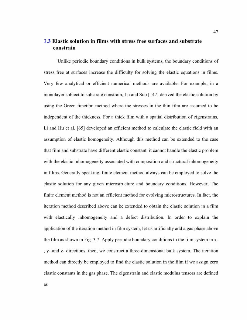
Fig. 3.7 Schematic drawing of an elastically inhomogeneous system. 49

Fig. 3.8 The image dislocation in the gas phase and the real dislocation below the

surface forms a dislocation loop. 51

Fig. 3.9 Gzxx /)(σ along AA − line shown in Fig.3.8. 52

Fig. 3.10 Gzzz /)(σ along AA − line shown in Fig.3.8. 53

Fig. 4.1 The precipitate shape as a function of time for a soft precipitate

( 40,3.0 == Rβ ). 61

Fig. 4.2 Evolution of compositional profiles as a function of time for a soft precipitate

( 40,3.0 == Rβ ), (a) along the x-direction, (b) along the diagonal direction.

63

Fig. 4.3 The shape of an isolated precipitate as a function of elastic inhomogeneity, (a)

70.1=β , (b) 35.1=β , (c) 00.1=β , (d) 60.0=β , (e) 45.0=β , (f) 3.0=β .

64

Fig. 4.4 Young’s modulus as a function of direction: dot-dashed line—matrix; dashed

line—precipitate; and solid line—a homogeneous solution. (a) Homogeneous

bulk and shear moduli but inhomogeneous elastic anisotropy; (b) homogeneous

bulk modulus and anisotropy but inhomogeneous shear modulus; (c)

homogeneous shear modulus and anisotropy but inhomogeneous bulk

modulus. 67

xi

Fig. 4.5 Two-phase morphology as a function of elastic inhomogeneity caused by

different degrees of elastic anisotropy in the matrix and precipitate ( Pδ , Mδ ):

(a) (1.00, 1.00), (b) (1.14, 0.89), (c) (1.34, 0.79), (d) (1.63, 0.72), (e) (2.05,

0.66), (f) (2.80, 0.61). Both the bulk and shear moduli are homogeneous.

68


different shear moduli in the two phases (a) β = 1.0, (b) β = 1.2, (c) β = 1.5,

(d) β = 1.9, (e) β = 2.6, (f) β = 3.6. The precipitate and matrix have the same

bulk moduli and the same degree of elastic anisotropy. 69

Fig. 4.7 Temporal evolution during phase separation of a homogeneous solid solution

into a two phase mixture for the case of elastic inhomogeneity caused by

different shear moduli in the two phases, β = 2.6. The precipitate and matrix

have the same bulk moduli and the same degree of elastic anisotropy. 70


different bulk moduli in the two phases (a) 0.1/ =MP BB , (b) 5.1/ =MP BB .

The precipitate and matrix have the same shear moduli and the same degree of

elastic anisotropy. 71

Fig. 4.9 Simulation cell of a thin film system. 76

Fig. 4.10 Temporal morphological evolution during spinodal decomposition in a thin film

under a uniform substrate constraint. 80


with two interfacial dislocations in both x- and y- directions. 81

xii

Fig. 4.12 Composition profile along A-A line shown in Fig.4.11 during spinodal

decomposition. 82

Fig. 4.13 Microstructural patterns formed during spinodal decomposition with different

interfacial dislocation arrays. 83

Fig. 4.14 Effect of film thickness on microstructural patterns with eight interfacial

dislocations in both x- and y- directions. 84

Fig. 5.1 Schematic illustration of a dislocation loop located at the center of a 2D

computational cell. 94

Fig. 5.2 Comparison of dislocation stress distributions calculated from numerical and

analytical solutions along A-A line shown in Fig. 5.1, the solid lines for

analytical solution and the symbol lines for numerical solutions. 97

Fig. 5.3a Order parameter profiles under different applied stresses *31σ with a nonlinear

dependence of the dislocation eigenstrain on order parameter. 98

Fig. 5.3b Order parameter profiles under different applied stresses *31σ with the linear

expression of the dislocation eigenstrain on order parameter. 99

Fig. 5.4a Shear stress distributions along the slip plane for a moving dislocation with the

linear eigenstrain expression. 100

Fig. 5.4b Shear stress distributions along the slip plane for a moving dislocation with the

non-linear eigenstrain expression. 101

Fig. 5.5a Average velocity of a dislocation vs applied shear stress shows the effect of

discretization. 107

xiii

Fig. 5.5b Average velocity of a dislocation vs applied shear stress shows the effect of

different eigenstrain expressions. 108

Fig. 5.6a Average velocity of a dislocation as a function of 0* / LdMM = for different

overall compositions under an applied stress 04.0*31 =σ . 111

Fig. 5.6b Average velocity of a dislocation as a function of 0* / LdMM = for overall

composition 15.00 =c under different applied stresses. 112

Fig. 5.7 Solute atmosphere around a moving dislocation in a solid solution with overall

composition 15.00 =c . (a), (b) and (c) were obtained under applied stress

04.0*31 =σ and with =*M 0.005, 0.2 and 3.0 respectively; (d), (e) and (f) were

obtained with 5.0* =M under different applied stresses 0.06, 0.1 and 0.14,

respectively. 114

Fig. 5.8a Dislocation velocity under applied stress 1.0*31 =σ . 115

Fig. 5.8b Dynamic dragging stress of solute atmosphere under applied stress 1.0*31 =σ .

116

Fig. 6.1 Al rich portion of the Al-Cu phase diagram. 121

Fig. 6.2 Crystal structure of the stable and metastable phases observed during

precipitation in Al-Cu alloys (reconstructed from Hornbogen [93] ). 125

Fig. 6.3 Transimission electron microgragh associated with the maximum peak of

hardness in an Al-1.7at%Cu alloy aged at 190oC for 30 hours. The foils were

oriented along matrix

001 . (from Ringer et al [197]). 126

xiv

Fig. 6.4 (a) orientation relationship of a plate-like 'θ precipitate, (b) two different

interface configurations around the rim of the plate where the interface is

incoherent. 130

Fig. 6.5 Two possible locations for 'θ nucleation near a dislocation. 133

Fig. 6.6 Equilibrium shape of a precipitate from the Gamma plot and the Wulff

Construction. 136

Fig. 6.7 Hardness curves vs aging time (from Silcock [255]). 142

Fig. 6.8 (a) Coordinate system associated with 'θ , (b) Definition of ϕ which is used to

describe the interfacial energy and mobility anisotropies. 146

Fig. 6.9 Chemical free energies of α (FCC solid solution) and 'θ phases calculated

from equations (6.10) and (6.11) at different temperatures. 149

Fig. 6.10 The height of chemical potentials in two phase equilibrium system. 170

Fig. 6.11 One-dimensional model of a 'θ precipitate growth. 172

Fig. 6.12 Moving distance of the interface as a function of time, (a) vs t (b) vs t . 173

Fig. 6.13 Comparison of composition profiles obtained by the phase-field simulations and

analytical solutions at different times. 174

Fig. 6.14 Morphological evolution of a precipitate from an initially non-equilibrium

shape to equilibrium in the absence of elastic energy. 176

Fig. 6.15 Composition evolution, (a) along the long axis, and (b) along the short axis of

the elliptic precipitate in the absence of elastic energy. 177


shape to equilibrium in the presence of elastic energy. 179

xv


the elliptic precipitate in the presence of elastic energy. 180

Fig. 6.18 Morphological evolution of a single precipitate represented by the composition

field in the absence of elastic energy. The white line is a contour of

composition 03.0=c . 183


field in the presence of elastic energy. The white line is a contour of

composition 03.0=c . 184

Fig. 6.20 Composition evolution, (a) along the length direction, and (b) along the

thickness direction in the absence of elastic energy. 185


thickness direction in the presence of elastic energy. 186

Fig. 6.22 Lengthening and thickening of a precipitate. 187

Fig. 6.23 Lengthening and thickening of a precipitate at the growth stage. 188

Fig. 6.24 Lengthening and thickening of a precipitate without elastic energy and the

coherent interface is immobile. 189

Fig. 6.25 Lengthening and thickening of a precipitate with elastic energy and the

coherent interface is immobile. 190

Fig. 6.26 Coarsening of two precipitates in the absence of elastic energy. 192

Fig. 6.27 Coarsening of two precipitates in the presence of elastic energy. 193

Fig. 6.28 Growth of multi-precipitates in two dimensions. 198

Fig. 6.29 TEM graph of 'θ precipitates from Weiland [180]. 199

Fig. 6.30 Growth of two precipitates in three dimensions. 201

xvi

LIST OF TABLES

Table 3.1 Convergence of the iteration method 40

Table 6.1 Stress-free strain zε in terms of interface configurations m:n 129

Table 6.2 The dependence of maximum grid spacing on the height of potential f∆ 169

xvii

ACKNOWLEDGEMENTS

I would like to express my sincere gratitude to my advisor, Dr. Long-Qing Chen, for his

constant advice, guidance, encouragement and understanding through the course of my

graduate study at Penn State. I thank Dr. David J. Green, Dr. Qiang Du and Dr. Zi-Kui

Liu for serving on my Ph.D. committee and providing insightful comments. I would like

to thank Dr. Yu-Xi Zheng for the help in the phase plane analysis for the phase-field

model of dislocation dynamics. I am also grateful to our collaborators, Dr. Hasso

Weiland, Dr. Joanne L. Murray and Dr. Wang Wei at ALCOA, Dr. Chris Wolverton at

Ford Motor Company, Dr. Qiang Du, Dr. Zi-Kui Liu and Dr. Peng Yu at Penn State for

their helpful discussions. I wish to thank my labmates, Dr. Yulan Li, Dr. Jaiho Choi, Dr.

Dongjin Seol, Dr. Venugopalan Vaithyanathan, Dr. Jingzhi Zhu and others, for the

pleasant collaborations and many helpful discussions. I am grateful for the financial

supports from NSF and ALCOA for my research. Of course, I cannot forget my deep

gratitude to my wife Yulan and to my daughters Lina and Lisa for their love and support.

1

Chapter 1

Introduction

Many important properties of a material can be engineered by controlling its solid

state phase transformations and the accompanying microstructure evolution. Examples

include the improvement of mechanical properties through solid state precipitation

reactions in alloys such as Ni-based superalloys and age-hardened Al-alloys, the useful

dielectric properties and electro-mechanical coupling effects by manipulating phase

transitions in ferroelectric crystals, the memory effect of shape-memory alloys by

utilizing martensitic transformations. Essentially all solid state phase transformations

produce coherent microstructures at their early stages. In a coherent microstructure, the

lattice directions and planes are continuous across the interfaces separating the parent and

product phases or separating different orientation domains of the product phase. In order

to maintain this lattice continuity, the lattice mismatch between the product and parent

phases and among the orientation domains of the product phase must be accommodated

by elastic displacements of atoms from their equilibrium lattice positions. Therefore,

formation of coherent microstructures generates coherency elastic strain energy whose

magnitude depends on the degree of lattice mismatch, the elastic properties of both the

parent and product phases, and the shape and spatial distributions of coherent particles or

domains [1,2]. The coherency elastic strain energy not only affects the thermodynamic

equilibrium properties such as transformation temperature, equilibrium composition and

equilibrium precipitate shape but also kinetic properties such as interface mobility and

2

coarsening behavior [3-9]. There have been intensive theoretical studies and various

computational simulations on the effect of coherency elastic strain energy on the

morphology of a coherent microstructure and its coarsening behavior, and they have been

recently reviewed [3,4]. Structural defects such as dislocations, grain boundaries,

interfaces and free surfaces inevitably exist in a crystalline solid. The structural

distortions around defects generate a stress field which may compensate the coherency

stress field associated with the coherent microstructure. They may also dramatically

changes the atom mobility. For example, the diffusivity along free surface, grain

boundary and dislocation is often several orders larger than that in the corresponding

bulk. As a consequence, the presence of defects may affect the nucleation, growth and

coarsening [10–19]. Recrystallization is an excellent example of using a heterogeneous

nucleation on dislocations to refine the grain size [20-27]. Therefore, quantitative

understanding of the effect of coherency stresses and defects on thermodynamics and

kinetics in solid state phase transformations would provide a scientific basis for

controlling solid state phase transformation and obtaining desired properties of materials.

Phase-field method is based on a diffuse-interface description [28-30], which is

used for modeling and predicting complex microstructure evolutions on a mesoscopic

length scale in many important materials processes. In this method, an arbitrary

microstructure is described by a set of field variables that are spatially continuous and

time-dependent. There are two types of field variables, conserved and non-conserved.

Conserved variables have to satisfy the local conservation condition. The most familiar

example of conserved field variables is the concentration field characterizing composition

3

variation. The field variables that do not satisfy the local conservation condition are non-

conserved variables, for example, the well-defined physical order parameters in order-

disorder transformations which characterizes structural heterogeneity. Phase-field theory

assumes that the microstructure evolution takes place to reduce the total free energy,

including the bulk chemical free energy, interfacial energy, elastic energy and

electrostatic energy. Following non-equilibrium thermodynamics, the conserved field

variables satisfy the Cahn-Hilliard equation [31], and the non-conserved phase-field

variables satisfy the Allen-Cahn equation (also called the Time Dependent Ginzburg-

Landau equation) [32]. Therefore, modeling the microstructure evolution in the

framework of phase-field theory is reduced to finding the solutions of Cahn-Hilliard

and/or Ginzburg-Landau equations. When the Langevin noise terms associated with

thermal fluctuations in composition and lro (long-range order) parameters [33,34] are

introduced, nucleation phenomena could be simulated as well.

Throughout the past decade, the phase-field method has been extensively

employed to simulate microstructure evolutions during solid state phase transformations,

including spinodal decomposition [35-42], precipitation of an ordered phase from a

disordered matrix [43-46], cubic to tetragonal transformation [47-52], hexagonal to

orthorhombic transformations[53-56], grain growth[57-64], ferroelectric domain

formation [65-68], and martensitic transformation [69-70]. However, most existing

models are limited to bulk systems that are often assumed to be elastically homogeneous

and free of structural defects. Moreover, most existing models are qualitative and usually

employ model free energy functions and model parameters. In this thesis, phase-field

4

models are developed to simulate microstructure evolutions in an elastically

inhomogeneous system with structural defects such as dislocations and stress free

surfaces in film systems, dislocation dynamics in a single crystal with diffusive solutes

and precipitates, and θ’ precipitation in Al-Cu alloys which involves strongly interface

energy anisotropy and interface mobility anisotropy.

1.1 Research Objectives

Elastic properties in different phases are often different. The elastic

inhomogeneity could be very strong in many practical materials such as multi-void and

film materials. Like the elastic anisotropy, the elastic inhomogeneity modifies the

coherency stress field, and hence, affects the kinetics of microstructure evolution. The

main challenge is to efficiently and accurately calculate the coherency stresses and elastic

energy in an elastically inhomogeneous system. There have been a number of efforts to

incorporate elastic inhomogeneity in diffuse-interface models. Onuki et al. [35-37]

derived a first-order elastic solution assuming weak elastic inhomogeneity. The effect of

elastic inhomogeneity on the particle morphology [35-39] and coarsening process [38,39]

was studied with phase-field models in binary alloys. Schmidt et al. [71,72] studied the

equilibrium shape of a coherent precipitate using a boundary integral method with a

sharp-interface description. However, the temporal evolution of precipitate morphologies

through the diffusion transport of atoms was not considered. Jou et al. [73] examined the

temporal evolution of precipitate shapes in elastically inhomogeneous solids by

simultaneously solving a diffusion equation and elasticity equations using the boundary

5

integral method. Since the interfaces are considered to be sharp in the boundary integral

method, it is difficult to handle certain topological changes that take place, for example,

the formation and disappearance of interfaces during the initial stage of spinodal phase

separation and during precipitate coalescence and splitting. Leo et al. [74] developed a

diffuse-interface model for modeling the microstructure evolution in elastically

inhomogeneous systems by coupling the Cahn–Hilliard diffusion equation with elasticity

equations. In his method, the elasticity equations are numerically solved by a conjugate

gradient method (CGM) at any given moment during microstructure evolution. A similar

diffuse-interface model using CGM was proposed by Zhu et al. [75]. However, the

numerical results show that CGM has a slow convergence, consequently is not a very

efficient method for an application in a system with an evolving microstructure.

Khachaturyan et al. [76] developed an analytical solution with a perturbation method

(PM) and sharp-interface description. The strain energy is expressed as a sum of

multiparticle interactions between finite elements of the constituent phases, pair-wise,

triplet, quadruplet and so on, the n-particle interaction energy being related to the (n-2)th

order term in the Taylor expansion of the Green function with respect to the elastic

modulus misfit. The order of approximation required for a given system depends on the

desired accuracy and the degree of elastic inhomogeneity. However, a direct application

of the analytical elastic energy expression to numerical simulations of coherent

microstructure evolutions in elastically inhomogeneous systems is difficult since the

elastic strain energy involves multidimensional integrals in both real and Fourier spaces.

More recently, Wang et al [77-78] proposed a new method by coupling the Eshelby’s

equivalent inclusion concept and Time Dependent Ginzburg-Landau equation. This

6

method has an unknown tensor, i.e., the mobility coefficients in Time Dependent

Ginzburg-Landau equations. The efficiency of the method depends on the choice of the

unknown tensor as well as the microstructure.

In this thesis, an efficient iteration method is proposed to solve the mechanical

equilibrium equations in a solid with strongly elastic inhomogeneity. It can be easily

incorporated into phase field models, and can take into account elastic anisotropy,

strongly elastic inhomogeneity and any kind of structural transformations such as cubic to

tetragonal and hexagonal to orthorhombic. If a gas phase, where the elastic constants are

zero, is introduced into a film system, the elastic solution in the film with a rough surface

can be obtained with the iteration method. This enables phase-field model to simulate the

effect of elastic energy on microstructure evolutions in films.

It has long been recognized that structural defects such as dislocations play an

important role in diffusion processes and phase transformations in solids. For example,

the interaction between solute atoms and a dislocation results in solute segregation and

depletion, leading to the formation of so-called “Cottrell atmosphere” [79]. The

nucleation of new phases around dislocations is often observed in experiments. Cahn [80]

first studied the nucleation of a second-phase precipitate around a dislocation with a

theoretical model that a cylindrical nucleus was assumed to replace the dislocation core,

thus providing additional driving force for nucleation compared to that in the bulk.

Dollins [81] and Barnett [82] considered the nucleation of a coherent precipitate on an

edge dislocation under some assumptions such as elastic isotropy and dilatational lattice

7

mismatches between precipitates and the matrix. Xiao and Hassen [83] re-examined the

coherent nucleation problem near an edge dislocation by considering the effect of Cottrell

atmosphere on coherent nucleation. However, they again had to assume isotropic elastic

modulus for the solid solution and a spherical shape for the nucleus. To relax many of the

assumptions in the analytical theories and to study the kinetic diffusion process, there

have been a number of computer simulation models proposed. For example, Wang et al.

studied the segregation profile around an edge dislocation, and the effect of the

segregation on dislocation dynamics using a discrete Monte-Carlo model [84]. The

interactions between dislocations and coherent precipitates were studied by using the

discrete atom method (DAM) [85]. The effect of dislocations on the morphological

evolution during spinodal decomposition was investigated by Le´onard and Desai [86].

They directly introduced the analytical elastic solution of a dislocation into the Cahn–

Hilliard equation. In summary, the analytical and computational models reviewed above

employ the analytical elastic solution of a dislocation. Although convenient in the study

of the effect of static dislocations on phase transformations in two dimensions, it is

difficult to do so in three dimensions with these models. Furthermore, dislocations might

even move due to the elastic interaction between dislocations and the evolving

microstructure during phase transformations. Therefore, a more realistic three-

dimensional defect model needs to be developed.

In micromechanics [2], ‘eigenstrain’ has been used to describe the distortion

associated with crystal defects for a long time. In this thesis, defects will be introduced

into phase field models with the ‘eigenstrain’ concept, which demonstrates two main

8

advantages. One advantage is that it allows people to easily represent an arbitrary spatial

distribution of defects into the systems and efficiently obtain the elastic solution by

combining Khachaturyan’s microelasticity theory [1] and the iteration method developed

in this thesis. The other advantage is that defect dynamics, such as dislocation motion and

crack propagation, can be simulated in phase-field framework if the distribution of

defects is described by order parameter field variables, as shown by Wang et al [87, 88].

The well-known advantage of phase-field models is that it avoids explicitly

tracking a boundary in conventional sharp boundary models by using a diffuse-interface.

However, the drawback is that it is hard to use phase-field models quantitatively. The

limit for a quantitative simulation comes from two main challenges. One is that it is often

computationally too stringent to choose a small enough gradient energy or grid size to

resolve the desired sharp-interface limit of the phase-field model, even on computers of

today. This severely restricts the size of simulation cell. The other one is how to

incorporate thermodynamic data, kinetic data and material properties into a phase field

model. Progress has recently been made to overcome these difficulties in solidification

simulation. Karma and Rappel [89-90] developed a quantitative phase field model of

alloy solidification with equal thermal conductivities in the solid and liquid by using a

‘thin-interface’ analysis. Their results show that the model parameters from ‘thin-

interface’ analysis can map onto the standard set of sharp-interface limit, yield a much

less stringent restriction on the interface thickness, and eliminate interface kinetic effects.

Kim [91] developed a phase field model of alloy solidification that is free from the limit

in the interface thickness and correctly generates the solute trapping phenomena at high

9

interface velocity. However, solid state phase transformations often evolve strongly

elastic interaction, strong interface energy anisotropy and interface mobility anisotropy,

which causes difficulties in the development of a quantitative phase field model.

In Al-Cu alloys, metastable 'θ ( CuAl2 ) precipitates are one of the primary

strengthening precipitates [92-104]. The study of 'θ ( CuAl2 ) precipitation is interesting

because the anisotropy of interfacial energy and interface mobility, and lattice

mismatches affect the precipitation process, hence the microstructure and mechanical

properties. With a conventional phase-field model, Li and Chen [105] simulated stress-

oriented nucleation and growth of 'θ precipitates. Vaithyanathan, et al [106] fitted a

chemical free energy function based on first principle calculations. The effect of elastic

energy, interface energy anisotropy and interface mobility anisotropy on the morphology

and growth of 'θ precipitates are simulated. However, to correctly describe 'θ

precipitation, the following factors should be further taken into consideration.

'θ ( CuAl2 ) is a compound phase. Its chemical free energy is only defined at 3/1=c (the

mole fraction of Cu composition). The question is how to construct the total chemical

free energy of a system with compound phases. The experimental observations show that

'θ precipitates are plate-like with a flat and broad interface. This implies that the

expression of interface energy should have cusps according to the Wulff construction of

an equilibrium precipitate shape. In addition, in order to develop a quantitative phase-

field model, the relationship between phase-field model parameters and thermodynamic

10

and kinetic data should be established. In this thesis, Al-Cu alloy is considered as a model

alloy for describing and verifying a quantitative phase field model.

Good understandings of dynamic interactions among dislocations, solutes,

precipitates and other defects are important in developing high strength alloys. Within

the continuum mechanics framework, there has been tremendous amount of effort

devoted to dislocation dynamics. A number of analytical models based on the concept of

low energy dislocation structures [107], reaction-diffusion approach [108-112], the

concept of dislocation sweeping mechanism [113,114], and stochastic dislocation

dynamic description [115,116]) have been proposed. A common feature of these models

is that the behavior of a dislocation system is described in analogy to other physical

problems such as spinodal decomposition, oscillating chemical reactions at a continuum

level. The properties of individual dislocations are taken into account indirectly.

Computer simulations of discrete dislocation dynamics in 2D and 3D have also been

performed [117-123]. Due to the long-range nature of elastic interactions between

dislocations, the direct numerical integration of dislocation dynamic equations is a very

time-consuming process, and thus, the size of the simulation cell and the number of

dislocations is limited. Recently, a significant advance in the application of phase-field

models in dislocation dynamics was made by Wang et al [87,88]. In their phase-field

model, the dislocation loops are labeled by a set of order parameter field variables. The

temporal evolution of the order parameter fields, i.e., dislocation motion, is described by

the phenomenological Time Dependent Ginzburg-Landau (TDGL) equation. The results

show that both long-range elastic interactions among dislocations and short-range

11

interactions, such as multiplication and annihilation of dislocations, are taken into

account in the model.

In this thesis, a phase field model of alloy strengthening is developed by coupling

the phase-field model of dislocation dynamics with diffusive solutes, elastically

inhomogeneity and defects. A new eigenstrain function of dislocations is constructed

which can eliminate the dependence of Burgers vector on applied stresses in the original

phase field model of dislocation dynamics [87]. Using phase plane analysis in two

dimensions, a relationship between dislocation mobility, velocity and applied stresses is

established, which can be used to determine the mobility coefficient in the evolution

equations with dislocation mobility data calculated by molecular dynamic simulation,

first-principle calculation and experiments.

1.2 Thesis Outline

This thesis has been organized into 7 chapters.

Chapter 1 consists of an introduction to the significance of coherency stresses and

defects in solid state phase transformations, the application of phase-field models in solid

state phase transformations, followed by the research objectives and the thesis outline.

Chapter 2 presents a phenomenological description of the phase-field approach in

solid state phase transformations.

12

In Chapter 3, an iteration method is proposed to obtain the elastic solution in a

solid with strongly elastic inhomogeneity and an arbitrary spatial distribution of defects.

The accuracy and efficiency of the iteration method are verified by comparing to existing

analytical solutions.

In Chapter 4, phase-field models are developed to simulate spinodal

decomposition in a bulk system with strongly elastic inhomogeneity and in a thin film

with a periodic array of interfacial dislocations. The iteration method described in

Chapter 3 is employed to obtain the elastic solution. Morphological dependence of an

isolated precipitate and multi-precipitates on elastic inhomogeneity is simulated in two-

dimensions. Directional spinodal decomposition induced by the stresses of periodically

distributed interfacial dislocations is studied.

In Chapter 5, a phase-field model of dislocation dynamics in a fcc single crystal

with diffusive solutes and immobile defects is developed. One composition field variable

that describes the solute concentration, and 12 order parameter field variables describing

the dislocation spatial distribution of 12 dislocation slip systems are employed. As an

example of the potential application of the developed phase-field model in alloy

strengthening, it is used to study the interaction between moving dislocations and

diffusive solutes.

In Chapter 6, a phase-field model is described for studying the 'θ precipitation in

Al-Cu alloys. This model takes into account interface energy anisotropy, interface

13

mobility anisotropy and elastic energy. The relationships between phase-field model

parameters and material constants are established by analyzing the static and dynamic

solutions of the kinetic equations in one dimension, which is the basis for a quantitative

simulation. A systematical testing in 1D, 2D and 3D of the model is made.

Chapter 7 summarizes the contributions of this thesis to phase-field theory and

discusses future work directions.

14

Chapter 2

Phase-field Model

2.1 Phenomenological description of solid state phase transformations

In order to better understand the phase-field model of microstructure evolution

during solid state phase transformations, let us briefly review the phenomenological

description of solid state phase transformations (see [124,125] for details). In principle,

any solid-state phase transformation can be characterized by physically well-defined

order parameters that distinguish the parent and product phases. For example, the

magnitude of a long-range order parameter in order-disorder transformation is

proportional to the intensity of a superlattice reflection corresponding to the ordered

superstructure, and the order parameter for a ferroelectric phase transition is the local

polarization vector which is proportional to the relative displacement of opposite-charged

ions. Since solid state phase transformations always involve structural changes, the

transformation strain, which is a measure of the strain state of a crystal during a phase

transformation with respect to the parent phase, could be seen as an order parameter. For

phase transformations in a homogeneous system, the transformation strain is determined

by the constraint conditions. In stress free phase transformations the transformation

strain (also called eigenstrain or stress-free strain) is a secondary order parameter in a

sense that there is another primary physical order parameter which characterizes the

phase transformation. In other word, it is a function of the primary physical order

parameters.

15

In a phenomenological description, the local free energy function is typically

expressed as a polynomial of order parameters using a conventional Landau-type of

expansion. All the terms in the expansion are required to be invariant with respect to the

symmetry operations of the high-temperature phase. The dependence of a phase

transformation on strain is primarily determined by the coupling between the primary

order parameters and strains, which has been discussed in great detail in an excellent

textbook by Salje [126].

To illustrate the role of elastic strain in phase transformations in a homogeneous

system, let us consider a simple model system with two degenerate states for the product

phase [127]. With a clamped boundary condition, the transformation strains ijε are given

constants. The Helmholtz free energy density, f, of the homogeneous system is a function

of order parameter η and total strains, and expressed as

),( ijff εη= (2.1)

If Helmholtz free energy density f is expanded with respect to the order parameter to the

fourth order and to the strain to the second order. Including only terms in strain to second

order is equivalent to assuming linear elasticity. Assuming that the coupling between the

strain (εij) and the order parameter (η) is linear-quadratic, the thermodynamics of the

system can be described by

16

( ) klijijklijijco TTf εελεδγηβηηα21

41

21 242 +−+−= (2.2)

where 0α , β , and γ are phenomenological coefficients which can be obtained by fitting

experimentally measured or computed properties with a clamped boundary condition. ijδ

is the Kronecker-delta functions. ijklλ is the elastic modulus tensor.

The critical temperature, i.e., the temperature below which the high temperature

phase becomes unstable, is obtained from

( ) 020

2

2

=−−=

∂∂

=

ijijco TTf εγδαη η

(2.3)

where, Tc is the critical temperature at clamped boundary condition 0=ijijεδ . The

equilibrium value for the order parameter at 0=ijijεδ can be obtained from

0=∂∂ηf (2.4)

It is given as a function of temperature by

17

( ) βαη coeq TT −±= (2.5)

Minimizing the Helmholtz free energy with respect to strain ijε

0=∂∂

ij

fε

(2.6)

we have

2γηδε klijklij s= (2.7)

where ijkls is the inverse elastic compliance tensor. With a linear elastic approximation,

the stress and elastic strain, eijε , satisfy the following relation ship

eij

ijfε

σ∂∂

= (2.8)

The elastic strain is equal to the difference between total strain (transformation strain in

this case) and eigenstrain,

0ijij

eij εεε −= (2.9)

18

Equations (2.6-2.9) illustrate that Helmholtz free energy reaches the minimum when the

transformation strain ijε is exactly equal to the stress free strain 0ijε . This means that the

phase transformation occurs under stress free boundary conditions. Therefore, the stress-

free strain reads

20 γηδεε klijklijij s== (2.10)

where ijkls is the compliance tensor.

Substituting the strain, ijε , into expression (2.2), the free energy as a function of

order parameter at stress free can be expressed as

( ) 42 '41

21 ηβηα +−= co TTf (2.11)

where klijklij s δδγββ 22' −= . In equation (2.11), 0α and 'β should be measured at

stress-free boundary conditions. cT should be measured at the clamped boundary

condition ( 0=ijε ).

With equation (2.11), the free energy at the clamped boundary condition, i.e., a

given strain state, can be rewritten as

19

( ) ( )( )oklkl

oijijijklco TTf εεεεληβηα −−++−=

21'

41

21 42 (2.12)

Equation (2.2) and (2.12) are equivalent. From equations (2.3 and 2.12), it can be found

that the clamped boundary condition affects the transformation temperature

oijijcTT αεδ /2+= (2.13)

One can also formulate the local free energy as a function of order parameter at a

given stress state since

( ) ( )( ) ijijoklkl

oijijijklco TTf εσεεεεληβηα −−−++−=

21'

41

21 42 (2.14)

where ijσ is the stress. Eliminating ijε from the equation (2.14), we have the free energy

at a given stress state ijσ ,

( )

( ) 242

42

21'

41

21

21'

41

21

γηδσσσηβηα

εσσσηβηα

klijklijklijijklco

oijijklijijklco

ssTT

sTTf

−−+−=

−−+−= (2.15)

20

It is evident that an applied stress will affect the critical temperature because 0ijε is a

quadratic function of η . Therefore, the transformation temperature depends on both the

clamped boundary conditions and applied stresses.

The shift from a chemical spinodal to a coherent spinodal is another example on

the effect of elastic strain on phase transformations [3,31,128]. In a solid solution, the

lattice parameter is a function of composition. For a cubic crystal, the stress-free strain

can be written in terms of composition c as,

)( 000 ccijij −= δεε (2.16)

where 0c is the composition of the reference state, dcda

a00

1=ε , a and 0a are lattice

constant corresponding to composition c and 0c , respectively. Under clamped boundary

conditions, elastic energy density due to the change in composition from the 0c can be

calculated by [3]

20

20 )(

112 cc

vvE −

−+

= εµ (2.17)

where µ is the shear modulus, ν the Poisson’s ratio. The total free energy density

includes chemical free energy of the solute solution )(0 cf and the elastic energy

21

20

200 )(

112),(),( cc

vvTcfTcf −

−+

+= εµ (2.18)

The phase boundary between stable (including metastable) and unstable states is

determined by the condition,

0114

),(),( 202

02

2

2

=−+

+∂

∂=

∂∂ εµ

vv

cTcf

cTcf (2.19)

The spinodal given by (2.19) is called the coherent spinodal. While the spinodal (without

any strain effect) which is given by

0),(

20

2

=∂

∂c

Tcf (2.20)

is sometimes called the chemical spinodal [3]. It can be seen that the coherent spinodal

differs from the chemical spinodal. When the system is inside the spinodal region,

0),(

20

2

<∂

∂c

Tcf and 0

114 2

0 >−+ εµ

vv (2.21)

22

The former promotes phase decomposition while the latter depresses it. Therefore,

spinodal decomposition accompanied by elastic strain does not always take place

throughout the chemical spinodal region. The chemical spinodal is shifted to a lower

temperature due to elastic energy.

In actual metallic materials, the effect of elastic energy on phase transformation

could be more complicated. The reason is that actual metallic materials are, in general,

anisotropic and inhomogeneous arising from crystal structural anisotropy and

inhomogeneity, composition inhomogeneity and the presence of structural defects. It is

commonly accepted that the elastic energy might affect transformation temperature,

critical nucleus size, precipitate morphology, precipitate arrangement, equilibrium

composition, and kinetics of phase transformations. One of the main objectives of the

present thesis is to study the effect of elastic energy on phase separation in bulk and thin

solid films.

2.2 Phase-field model of solid state phase transformations

Microstructures are compositional and structural inhomogeneities that arise from

processing of materials [129]. To model microstructure evolution during solid state phase

transformations, one can simply extend the above phenomenological description of solid

state phase transformations in homogeneous systems to inhomogeneous systems. In a

heterogeneous microstructure, both the order parameters (and/or composition) and the

strain (or stress) are space-dependent. A phase-field model describes a microstructure by

23

using a set of field variables that might be composition, order parameter, polarization

vector and orientation. There are two types of field variables, conserved and non-

conserved. Conserved variables have to satisfy the local conservation condition like

composition. The field variables are continuous across the interfacial regions. In a phase-

field model, the total free energy of an inhomogeneous microstructure system described

by a set of conserved field variables ( Nccc ,,, 21 L ) or/and non-conserved ( pηηη ,,, 21 L )

field variables is given by

( ) ( )

( ) ,'

,,,,,,,E11

22121

∫∫

∫ ∑∑

+

∂

∂

∂

∂+∇+=

==

xxdd'-G

xdxx

ccccf

33

3P

p j

p

i

pij

N

nnnPN

xx

ηηβαηηη LL

(2.22)

where f is the local free energy density which defines the fundamental thermodynamics

of the system. The gradient energy terms in the first volume integral, which are local

contributions to the free energy, describe the interaction between long-wave fluctuations

in adjacent finite volumes and are responsible for the field continuity. The gradient

energy coefficients nα and ijβ are related to interfacial energy and interface thickness.

Therefore, the first volume integral represents the contribution from local and short-range

chemical interactions. The second integral represents the contributions from long-range

interactions, such as elastic interactions, electric dipole-dipole interactions and

electrostatic interactions. The temporal and spatial evolution of the field variables is

24

governed by the reduction of the total free energy, and described by the Cahn-Hilliard

nonlinear diffusion equation [130] for conserved field variables

),(),(

),( txtxc

EMt

txci

jij

i ξδδ

+∇=∂

∂ (2.23)

and the Ginzburg-Landau equation [32] for non-conserved field variables

),(),(

),(t

tEL

tt

pq

pqp x

xx

ζδη

δη+−=

∂

∂ (2.24)

where ijM and pqL are related to atom or interface mobility, and iξ and pζ are the noise

terms. The origin of the noise terms comes from the microscopic degrees of freedom, i.e.,

from the thermal vibrations (phonons) and/or high-order correlations with short

relaxation time. The noise terms, which aid in the nucleation of precipitates [131,132],

are random numbers with Gaussian distributions, and their correlations satisfy

requirements of the fluctuation-dissipation theorem [133].

For a given system under consideration, once the total free energy is formularized,

modeling the microstructure evolution in the framework of phase-field theory is

essentially reduced to find the solutions of Cahn-Hilliard and/or Ginzburg-Landau

equations under initial and boundary conditions. In principle, the local free energy

function can be obtained from thermodynamic calculations and data from atomic scale

25

simulations such as first principle calculations and molecular dynamic simulations, and

experiments. All phenomenological model parameters ( nα , ijβ , ijM and pqL ) can be

calculated with the relationships between model parameters and material properties,

which can be derived by theoretical analysis of equilibrium solutions and dynamic

solutions (see section 6.2 for details). Most existing phase-field models employ model

free energy functions; see recent review papers [8] for details of free energy constructions

and the calculations of long-range interaction energies in most important applications of

phase-field models.

26

Chapter 3

Elastic Solution in a Solid with Strongly Elastic Inhomogeneity and Arbitrary Spatial Distribution of Defects

Microstructure evolution takes place to reduce the total free energy that may

include the bulk chemical free energy, interface energy, elastic energy, and/or under

applied external fields such as applied stresses [129]. In a coherent microstructure, the

elastic energy arises from lattice mismatches is often comparable to the change in the

interface energy or chemical free energy. Therefore, an efficient and accurate method to

calculate the elastic energy is desirable for predicting microstructure evolutions. A

number of calculation methods of elastic energy in a solid with an evolving

microstructure were developed, which have been reviewed in the introduction. In this

chapter, an accurate and efficient iteration method is proposed to calculate the elastic

energy in a solid with strongly elastic inhomogeneity and arbitrary spatial distribution of

defects during solid state phase transformations. It is quite convenient to incorporate this

method into phase-field models. Furthermore, the elastic energy in a film subject to

substrate constraint can also be obtained with the iteration method if a gas phase, where

the elastic constant is zero, is introduced [134-136]. Thus, the application of phase-field

models can be extended to an entirely new research field: the effect of elastic energy on

microstructure evolutions in thin films.

27

3.1 Mechanical equilibrium equations

To present the method of solving the elastic problem in a solid with elastic

inhomogeneity and arbitrary spatial distribution of defects, we take a binary solid

solution with a compositional inhomogeneity )(xc as an example, where )(xc is the

mole or atom fraction at position x . The local elastic modulus tensor is assumed to be a

linear function of the compositional inhomogeneity through [137]

meq

peq

meqp

ijklmeq

peq

peqm

ijklijkl

xxx

cccc

cccc

−

−+

−

−=

)()()( λλλ (3.1)

where mijklλ and p

ijklλ are the elastic modulus tensors for the matrix with equilibrium

composition mepc and for the precipitate with equilibrium composition p

epc , respectively. It

is easy to show that the local elastic modulus tensor (3.1) can be rewritten as

)()( '0 xx ijklijklijkl cδλλλ += (3.2)

where 0)()( ccc −= xxδ , 0ijklλ is a constant representing the elastic modulus tensor for a

homogeneous solid solution with composition 0c , and 'ijklλ is given by

meq

peq

mijkl

pijkl

cc −

− λλ . We

assume that the local stress-free strain tensor can be described in terms of the

compositional inhomogeneity ))(,( xxcik cε . If the variation of stress-free lattice

28

parameter, a, with composition obeys the Vegard’s law, the local stress-free strain

associated with the compositional inhomogeneity is given by,

ijcij xxx δδεε )())(,( 0 cc = (3.3)

where dcda

a1

0 =ε is the composition expansion coefficient of the lattice parameter and

ijδ is the Kronecker–Delta function

Most structural defects such as dislocations, grain boundaries, cracks and slip

bands can be introduced into a phase-field model using their corresponding spatially

dependent stress free strain [2,87,88,138-142]. For the case of dislocations, the stress

field of a dislocation loop on slip plane p with a Burgers vector b, is described by the

stress free strain,

)())(21)( 0

0

xxxdisij −+= δε b(j)n(ib(i)n(j)

d (3.4)

where n is the unit vector normal to the slip plane, 0d is the interplanar spacing of the

slip planes, )( 0xx −δ is the Dirac delta function and 0x is a point inside the dislocation

loop on the slip plane. For a spatial distribution of many dislocation loops, the total stress

free strain can be obtained by adding the stress free strain of individual dislocation loops.

29

We use )(xdisijε to denote the total stress free strain due to the spatial distribution of

dislocations or other defects. Therefore, the total stress free strain associated with the

composition inhomogeneity and defects can be written as

)()()(0 xxx disij

cijij εεε += (3.5)

Let’s use )(xijε to denote the total strain measured with respect to a reference

lattice and assume linear elasticity, the Hooke’s law gives the local elastic stress,

)]()()][([ 0'0 xxx klklijklijklelij εεδλλσ −+= c (3.6)

During the evolution of composition and defects, since the mechanical equilibrium with

respect to elastic displacements is usually established much faster than any material

processes, for any given distribution of composition, the system is always at mechanical

equilibrium,

0=∂

∂

j

elij

xσ

(3.7)

where jx is the jth component of the position vector, x . Following Khachaturyan

[143,144], the total strain )(xijε may be represented as the sum of homogeneous and

heterogeneous strains:

30

)()( xx ijijij δεεε += (3.8)

where the homogeneous strain, ijε , is defined so that

0)( =∫ xd 3

vij xδε (3.9)

The homogeneous strain is the uniform macroscopic strain characterizing the

macroscopic shape and volume change associated with the total strain, )(xijε .let us use

)(xiu to denote the ith component of displacement of heterogeneous deformation.

According to the relationship of strain and displacement, the heterogeneous strain can be

expressed as,

∂

∂+

∂∂

=k

l

l

kkl

xxxx

ux

u )()(21)(δε (3.10)

Substituting equations (3.4-6) and (3.10) to the mechanical equilibrium equation (3.7),

one has

31

])()][([

)())((

0'0

'2

0

klklijklijklj

klj

ijkllj

ijkl

xx

xx

εεδλλ

δλλ

−+∂∂

=

∂∂

∂∂

+∂∂∂

cx

ux

cxxx

(3.11)

The determination of the equilibrium elastic field for an elastically inhomogeneous solid

with spatial arbitrary distribution of defects is reduced to solving the mechanical

equilibrium equation (3.11) subject to appropriate boundary conditions.

3.2 Elastic solution in bulk systems with periodic boundary conditions

With periodic boundary conditions, Fourier transforms method can be employed

to solving the mechanical equilibrium equation (3.11).

3.2.1 Zeroth-order approximation

Because of the non-linearity of the mechanical equilibrium equation (3.11), in

general, it cannot be solved analytically. However, if one ignores the elastic modulus

inhomogeneity, 0' =ijklλ , the mechanical equilibrium equation becomes linear and is

given by

j

klijkl

lj

kijkl xxx

u∂

∂=

∂∂∂ )()( 0

002

0 xx ελλ (3.12)

32

where )(0 xku denotes the kth component of the displacement in the zeroth order

approximation and Equation (3.12) can be readily solved in the Fourier space [144],

)()()( 000 ggg mnijmnjikk giGv ξλ−= (3.13)

where )(0 gkv and )(0 gmnξ are Fourier transforms of )(0 xku and )(0 xmnε , respectively, g is

a reciprocal lattice vector, jg is the jth component of g, and )(gikG is the inverse tensor

to ljijklik nngG 021 ))(( λ=− g with ggn = . The back Fourier transform of )(0 gkv gives the

real-space solution for the displacement field in the zeroth order approximation,

ggx x 303

0 )()2(

1)( devu igkk

⋅∫=π

(3.14)

3.2.2 First-order approximation

With the zeroth-order solution, one can analytically obtain the solution or the

displacement field with a first-order approximation. To do this, we replace the

displacement in the nonlinear term in equation (3.11) using the zeroth order solution and

move it to the right-hand side,

33

∂

∂∂∂

−−+∂∂

=∂∂

∂

l

k

jijklklklijklijkl

jlj

kijkl x

uc

xc

xxxu )(

)(])()][([)( 0

'0'012

0 xxxxxδλεεδλλλ (3.15)

where )(1 xku represents the kth component of displacement in the first-order

approximation. Equation (3.15) has essentially the same structure as equation (3.12)

except for a slightly more complicated right-hand side in equation (3.15). Therefore, the

solution )(1 xku can also be analytically obtained using Fourier transforms, i.e.

g

xxxxgg

∂

∂−−+−=

n

mijmnmnmnijmnijmnjikk x

uccgiGv

)()(])()][([)()(

0'0'01 δλεεδλλ (3.16)

A significant difference between equation (3.12) and equation (3.15) is the fact that the

homogeneous strain, klε enters equation (3.15). As a result, with a first-order

approximation, an applied strain or stress will affect the heterogeneous elastic

displacements.

3.2.3 High-order approximations

Higher order solutions for )(xnku can be obtained using an iteration process. For

example, the nth order solution for displacement, )(xnku , can be obtained from the

following equation,

34

∂

∂∂∂

−−+∂∂

=∂∂

∂ −

l

nk

jijklklklijklijkl

jlj

nk

ijkl xu

cx

cxxx

u )()(])()][([

)( 1'0'0

20 xxxxx

δλεεδλλλ 3.17)

where )(1 x−nku is the solution from a lower-order approximation. Again the elastic

displacement in the nth order approximation can be obtained from equation (3.17) using

Fourier transforms.

3.2.4 Elastic energy

The elastic strain energy density for a given compositional distribution in an

elastically inhomogeneous is given by

)]()()()][()()([

)]([21

21 '0

xxxxxx

xe

dkl

cklklij

dij

cijijij

ijklijklelkl

elijijklel

εεδεεεεδεε

δλλεελ

−−+−−+

+== c (3.18)

The total strain energy is given by

xdeEv

elel3∫= (3.19)

In equation (3.18), )(xklδε is given by

[ ] gggx xg 33 )()(

2)2(1)( degvgvi i

ijjiij⋅+= ∫π

δε (3.20)

35

where )(giv is the ith component of the displacement. The corresponding elastic stress is

given by equation (3.6). The homogeneous strain in equation (3.15) and equation (3.8) is

determined by the boundary constraint. If the boundary is clamped so that the system is

not allowed to have any homogeneous deformation, the homogeneous strain, ijε is equal

to zero. Similarly, if the system is subject to an initial applied strain, aijε , then the

boundary is held fixed, aijij εε = . On the other hand, if the system is stress-free, i.e., the

system is allowed to deform so that the average stress in the system is zero, the

homogeneous strain is obtained by minimizing the total elastic energy with respect to the

homogeneous strain [145].

3.2.5 Verification of the iteration method in bulk systems

Here, the convergence and accuracy of iteration method are examined

systematically. In principle, the efficiency and accuracy of the proposed iteration method

for a given order of approximation can be tested with analytical solutions which are

available for certain special precipitate shapes [2]. However, the analytical solutions are

available only for systems with a sharp-interface description whereas the interfaces in our

numerical calculation are diffuse. Therefore, to examine accuracy, we compare the results

from the proposed method with those obtained from an independent calculation using a

conjugate gradient method (CGM) with the same diffuse-interface description [75]. In

CGM, the elastic equation is numerically solved until the results converge.

36

For the sake of simplicity, we consider a two dimensional model binary alloy with

its chemical thermodynamics described by the following local incoherent free energy

density,

42 )5.0(5.2)5.0()( −+−−= cccf , (3.21)

where c is the composition. The equilibrium compositions determined from equation

(3.21) are 0.053 and 0.947, respectively. We introduce a circular precipitate with

composition 0.947 and a radius of xR ∆= 10 in a square domain of matrix

( xx ∆×∆ 256256 ) with composition 0.053. x∆ is the dimensionless grid spacing. Periodic

boundary conditions are applied along both Cartesian axes. The initially sharp

composition profile describing the precipitate is allowed to relax for a certain number of

time steps by solving the Cahn–Hilliard diffusion equation (4.5) with a gradient energy

coefficient 5.10 =κ , but without including the stress effect. The resulting two-

dimensional diffuse compositional profile is then used to calculate the stress distributions

using the proposed iteration method with different orders of approximation and the CGM

[75]. For comparing the results, the number of time steps to relax the profile is not

particularly important since we use the same profile for the two independent calculations.

Both calculations employed the spectral method for the spatial discretization of the

elasticity equation. The composition expansion coefficient, 0ε , is chosen to be 0.05. The

elastic constants used are 300011 =C , 1000

12 =C , 100044 =C for the matrix; 150'

11 =C ,

37

50'12 =C , 50'

44 =C for hard precipitates and 150'11 −=C , 50'

12 −=C , 50'44 −=C for soft

precipitates, all in units of TkN BV . ijC and 'ijC is the elastic stiffness in Voigt’s notation.

This set of elastic constants produce more than 50% difference in the elastic constants

between the precipitate and matrix, which is artificially large compared to the typical

elastic inhomogeneity in most of the practical two phase alloys.

Examples of equilibrium stress distributions, ( )11σσ =xx and ( )22σσ =yy , as a

function of position along a line cut through the center of the precipitate in the 1x

direction are shown in Fig. 3.1 for a hard precipitate, and Fig. 3.2 for a soft precipitate.

The shear component, ( )12σσ =xy , is zero along the line, so it is not shown. In both Fig.

3.1 and 3.2, the squares and circles represent the results from the proposed perturbation

method and the crosses and pluses represent those from the CGM. It can be seen that for

both hard and soft precipitates, the results from two calculations agree very well for both

stress components. Both calculations converge to essentially the same results although

the two calculations were performed using two entirely independent computer codes. It is

shown that although the stresses in the matrix are similar for both the hard and soft

precipitates, the absolute magnitude within the hard precipitate is significantly higher

than that within the soft precipitate. It is easily understandable since we used exactly the

same two-dimensional compositional profile for the hard and soft precipitates and the

larger elastic constants for the hard precipitates would produce larger stresses. To

examine the convergence of the elastic solution as a function of iteration number, or the

order of approximation, the stress components, xxσ and yyσ , as a function of position for

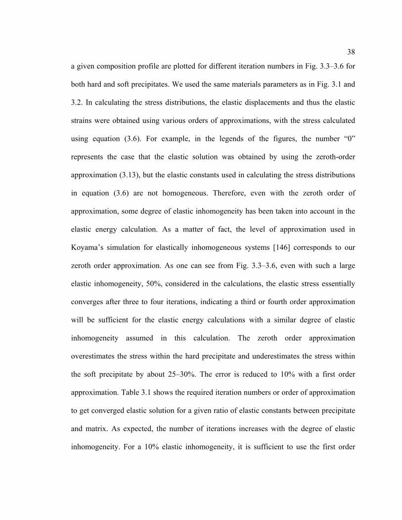
38

a given composition profile are plotted for different iteration numbers in Fig. 3.3–3.6 for

both hard and soft precipitates. We used the same materials parameters as in Fig. 3.1 and

3.2. In calculating the stress distributions, the elastic displacements and thus the elastic

strains were obtained using various orders of approximations, with the stress calculated

using equation (3.6). For example, in the legends of the figures, the number “0”

represents the case that the elastic solution was obtained by using the zeroth-order

approximation (3.13), but the elastic constants used in calculating the stress distributions

in equation (3.6) are not homogeneous. Therefore, even with the zeroth order of

approximation, some degree of elastic inhomogeneity has been taken into account in the

elastic energy calculation. As a matter of fact, the level of approximation used in

Koyama’s simulation for elastically inhomogeneous systems [146] corresponds to our

zeroth order approximation. As one can see from Fig. 3.3–3.6, even with such a large

elastic inhomogeneity, 50%, considered in the calculations, the elastic stress essentially

converges after three to four iterations, indicating a third or fourth order approximation

will be sufficient for the elastic energy calculations with a similar degree of elastic

inhomogeneity assumed in this calculation. The zeroth order approximation

overestimates the stress within the hard precipitate and underestimates the stress within

the soft precipitate by about 25–30%. The error is reduced to 10% with a first order

approximation. Table 3.1 shows the required iteration numbers or order of approximation

to get converged elastic solution for a given ratio of elastic constants between precipitate

and matrix. As expected, the number of iterations increases with the degree of elastic

inhomogeneity. For a 10% elastic inhomogeneity, it is sufficient to use the first order

39

approximation. Even with inhomogeneities as large as 100%, it requires only about five

iterations.

40

Table 3.1 Convergence of the iteration method

Mij

Pij

CC

0.19 0.37 0.55 0.73 0.91 1.00 1.09 1.27 1.45 1.63 1.99

Iterations 5 4 3 2 1 0 1 2 3 4 5

41

Fig. 3.1 Stress distributions along the x-direction across the center of a hard precipitate.

The open squares and circles represent the xxσ and yyσ components obtained from the

proposed iteration method. The crosses and pluses represent the corresponding results

from a conjugate gradient method (CGM).

42

Fig. 3.2 The xxσ component of the elastic stress along the x direction across the center

of the hard precipitate as a function of iteration numbers (or the order of approximations)

from the perturbation iterative method.

43

Fig. 3.3 Stress distributions along the x-direction across the center of a soft precipitate.

The open squares and circles represent the xxσ and yyσ components obtained by the

proposed iteration method. The crosses and pluses represent the corresponding results

from a conjugate gradient method (CGM).

44


hard precipitate as a function of iteration numbers (or the order of approximations) from

the iterative method.

45

Fig. 3.5 The xxσ component of the stress along the x-direction across the center of the

soft precipitate as a function of iteration numbers (or the order of approximations) from


46


soft precipitate as a function of iteration numbers (or the order of approximations) from


47

3.3 Elastic solution in films with stress free surfaces and substrate constrain

Unlike periodic boundary conditions in bulk systems, the boundary conditions of

stress free at surfaces increase the difficulty for solving the elastic equations in films.

Very few analytical or efficient numerical methods are available. For example, in a

monolayer subject to substrate constrain, Lu and Suo [147] derived the elastic solution by

using the Green function method where the stresses in the thin film are assumed to be

independent of the thickness. For a thick film with a spatial distribution of eigenstrains,

Li and Hu et al. [65] developed an efficient method to calculate the elastic field with an

assumption of elastic homogeneity. Although this method can be extended to the case

that film and substrate have different elastic constant, it cannot handle the elastic problem

with the elastic inhomogeneity associated with composition and structural inhomogeneity

in films. Generally speaking, finite element method always can be employed to solve the

elastic solution for any given microstructure and boundary conditions. However, The

finite element method is not an efficient method for evolving microstructures. In fact, the

iteration method described above can be extended to obtain the elastic solution in a film

with elastically inhomogeneity and a defect distribution. In order to explain the

application of the iteration method in film system, let us artificially add a gas phase above

the film as shown in Fig. 3.7. Apply periodic boundary conditions to the film system in x-

, y- and z- directions, then, we construct a three-dimensional bulk system. The iteration

method can directly be employed to find the elastic solution in the film if we assign zero

elastic constants in the gas phase. The eigenstrain and elastic modulus tensors are defined

as

48

+=

substrateandfilminphasegasthein

disij

cij

disij

ij )()()(

)(0

xxx

xεε

εε (3.22)

and

+=+=

substrateandfilminphasegasthein

ijklijklijklijklijkl )(

0.0)()( '0

'0

xxx

λλλλλ (3.23)

where )(xdisijε is the eigenstrain associated with the distribution of real dislocations in the

solid and image dislocations in the gas phase, )(xcijε is the eigenstrain associated the

composition inhomogeneity, )(0 xijε in the total eigenstrain. )(0 xijklλ is the elastic constant

of one of the phases in the system, )(' xijklλ is the change in elastic constants with respect

to )(0 xijklλ . Notice that the elastic constant is zero in the gas phase, so all stress

components are zero in the gas phase. From the continuity of stresses at the interface

between gas phase and solid phase, the elastic solution obtained satisfies the stress-free

boundary conditions at the surface of the film ( fhzx ==3 ), and the bottom of the

substrate ( shzx ==3 ). In this thesis, we assume the film and substrate are elastic

homogeneous, i.e., )(' xijklλ =0, and the surface is flat. The iteration method has been

employed to simulate the formation of quantum dots where the surface is rough [4].

49

Fig. 3.7 Schematic drawing of an elastically inhomogeneous system.

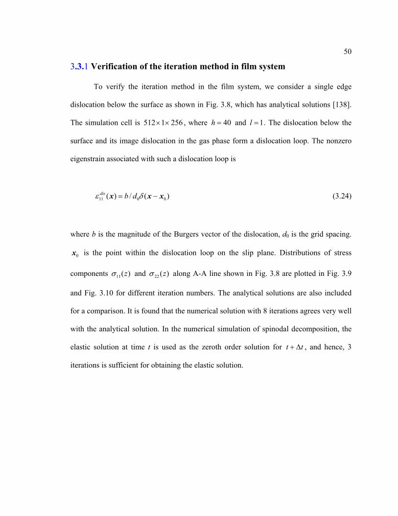
50

3.3.1 Verification of the iteration method in film system

To verify the iteration method in the film system, we consider a single edge

dislocation below the surface as shown in Fig. 3.8, which has analytical solutions [138].

The simulation cell is 2561512 ×× , where 40=h and 1=l . The dislocation below the

surface and its image dislocation in the gas phase form a dislocation loop. The nonzero

eigenstrain associated with such a dislocation loop is

)(/)( 0011 xxx −= δε dbdis (3.24)

where b is the magnitude of the Burgers vector of the dislocation, d0 is the grid spacing.

0x is the point within the dislocation loop on the slip plane. Distributions of stress

components )(11 zσ and )(22 zσ along A-A line shown in Fig. 3.8 are plotted in Fig. 3.9

and Fig. 3.10 for different iteration numbers. The analytical solutions are also included

for a comparison. It is found that the numerical solution with 8 iterations agrees very well

with the analytical solution. In the numerical simulation of spinodal decomposition, the

elastic solution at time t is used as the zeroth order solution for tt ∆+ , and hence, 3

iterations is sufficient for obtaining the elastic solution.

51

Fig. 3.8 The image dislocation in the gas phase and the real dislocation below the

surface forms a dislocation loop.

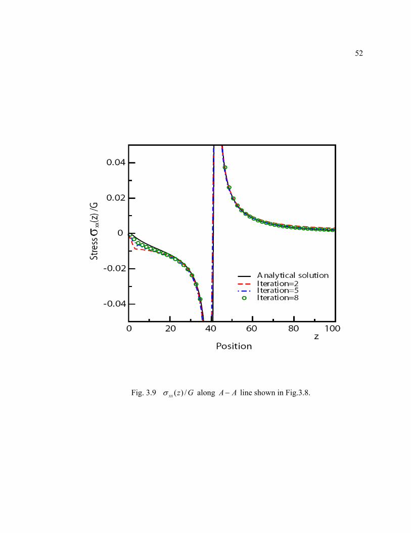
52

Fig. 3.9 Gzxx /)(σ along AA − line shown in Fig.3.8.

53

Fig. 3.10 Gzzz /)(σ along AA − line shown in Fig.3.8.

54

3.4 Conclusion

For an elastically inhomogeneous bulk or film system with spatial arbitrary

defects, an iteration method is proposed to calculate the elastic energy. The accuracy and

the efficiency of the iteration method are numerically verified by comparing the

analytical solution of testing problems. The numerical results demonstrate that once the

0ijklλ are set to be the elastic constant of the hardest phase in the elastically

inhomogeneous system the iteration method is always convergence, and 5~8 iterations

even for strongly elastic inhomogeneity can give a good elastic solution. For the

application of the iteration method for solving the elastic solution in evolving

microstructures, 2~3 iterations are sufficient to obtain the elastic solution for a updated

microstructures. Therefore, the iteration method is a very efficient approach for the

simulation of microstructure evolutions. The defects are introduced by using the concept

of “eigenstrains” in micromechanics which allow that the elastic fields from structural

defects and coherent compositional/structural inhomogeneity are obtained within exactly

the same formulation in the framework of Khachaturyan’s microelasticity theory.

55

Chapter 4

Spinodal Decomposition in Bulk and Film Systems

In spinodal decomposition, phase separation occurs by the spontaneous

amplification of compositional fluctuations when a homogeneous solute solution is

quenched to the unstable part of a miscibility gap. Because the two phases form by a

continuous process they start out coherent with one another [147]. If the elastic constant

is a function of composition, one phase becomes gradually harder and harder while the

other phase becomes softer and softer during the spinodal decomposition. It is evident

that the coherency stress field depends on the degree of such an elastic inhomogeneity.

Therefore, the elastic inhomogeneity will affect the kinetics of spinodal decomposition

and resulting patterns of separated phases. Furthermore, structural defects such as

dislocations exist inevitably in crystalline solids. For example, in a film deposited on

different substrates, a coherent interface becomes semi-coherent or incoherent by the

generation of interfacial dislocations as the lattice mismatch between the film and the

substrate increases. As a result, the uniform constraint stress field corresponding to the

coherent interface becomes a localized constraint stress field corresponding the

incoherent interface. If the film is unstable with respect to spinodal decomposition,

different patterns of separated phases may form due to the density and distribution of

interfacial dislocations.

56

Since Cahn first introduced the elastic energy term in the expression of the total

free energy of the system [148], there have been numerous studies on the

thermodynamics of coherent systems including the interaction of composition and stress

in crystalline solids [1, 149-153]. The effect of dislocations on the morphological

evolution during spinodal decomposition was investigated by Le´onard and Desai [154]

who directly introduced the analytical elastic solution of a dislocation into the Cahn–

Hilliard equation. Formulations for spinodal decomposition have recently been developed

especially for confined geometry such as thin films or plates in accordance with recent

interests in thin film applications of materials [155-157].

In this chapter, phase-field models are developed to simulate the spinodal

decomposition in a bulk system with strongly elastic inhomogeneity and in a thin film

with a periodic array of interfacial dislocations. The iteration method described in

Chapter 3 is employed to obtain the elastic solutions. Morphological dependence of an

isolated precipitate and multi-precipitates on elastic inhomogeneity is simulated in two-

dimensions. Directional spinodal decomposition induced by the stresses of periodic

distributed interfacial dislocations is studied.

4.1 Phase-field model of spinodal decomposition

We consider a binary solid solution which is unstable to spinodal decomposition.

One phase-field variable, ),( tc x , representing the mole or atom fraction at position x

and time t, is needed to describe the composition evolution or morphological evolution of

57

separated phases. For the elastic problem, the same notations and assumptions described

in section 3.2 and section 3.3 are applied. Then, the Helmholtz free energy of the system

includes three contributions: bulk chemical free energy, interfacial energy and elastic

energy,

xdttttcTtcfE klijijklv

322

)],(),(),(21)),((

2)),,(([ xxxxx εελκ

+∇+= ∫ . (4.1)

where ),( Tcf is the chemical free energy density of the solid solution, κ is the gradient

energy coefficient which is determined by the interfacial energy and thickness. The third

term in (4.1) is the elastic energy density.

Since the composition is a conserved field variable, the kinetic equation of the

composition field is described by the Cahn-Hilliard-type diffusion equation given by

),(),(),(

)),,((

),(),(

),(

22 ttctdc

TtcdfM

ttc

EMt

tc

el xxxx

xx

x

ξµκ

ξδδ

+

+∇−∇⋅∇=

+∇=∂

∂

(4.2)

where ),( txξ is the noise term representing composition fluctuation. M is chemical

mobility. If we assume that the atomic mobilities of species 1 and 2 are equal, the

mobility, M, is given by

58

TktctDcM

B

)),(1)(,( xx −= (4.3)

where D is the chemical diffusion coefficient, Bk is the Boltzmann constant and T is the

temperature. The mobility is further simplified by assuming that the factor

)),(1)(,( tctc xx − is a constant given by )1( 00 cc − where 0c is the overall composition.

elµ is the elastic potential due to the coherency strain and is given by [158]

20000'00'

'

00000000

))((23)())()((2

))())(()((21

)())()((

xxxx

xxx

xxx

cc

cN

klijijklklijdisijijijkl

klklijdisijijijkl

klijijklijijdisijijijklelV

δεελδεδεεελ

δεεδεεελ

δεελεδεεελµ

+++−

++++

++++−=

(4.4)

where vN is the number of atoms per unit volume, and ijij δεε 000 = .

The simulations are performed in two or three dimensions. In simulations,

periodic boundary conditions are employed. The elastic stress field is calculated by the

iteration method proposed in section 3.3. The chemical free energy density of the solid

solution is expressed by

42 )5.0),((5.2)5.0),(()),,(( −+−−= tctcTtcf xxx (4.5)

The equilibrium compositions determined from equation (4.5) are 0.053 and 0.947,

respectively. The evolution equation (4.2) is solved by semi-implicit schemes [159].

59

4.2 Spinodal decomposition in a bulk system

4.2.1 Morphological dependence of isolated precipitates on elastic inhomogeneity The shapes of a single coherent precipitate in elastically inhomogeneous systems

have been studied with boundary integral equation method [71,72] and discrete atom

method (DAM) [160]. With the phase-field model and the proposed iteration method, the

shape evolution of an isolated precipitate and its dependence on elastic inhomogeneity

are re-examined in this section. The shape evolution of an isolated particle towards

equilibrium is obtained by solving the Cahn–Hilliard diffusion equation (4.2). A

simulation cell of 256256× grids is used. A circular precipitate ( 40=R ) is placed in the

center of the simulation cell. The initial composition within the precipitate is assigned the

incoherent equilibrium value determined from the local free energy density function

),( Tcf , c = 0.947, whereas c = 0.06 in the matrix which is higher than the incoherent

equilibrium composition, 0.053. The coherent equilibrium compositions are not known in

advance and will be automatically achieved during the temporal evolution towards

equilibrium. The dimensionless time step for integrating the Cahn–Hilliard equation is

5.0)( 2

* =∆

∆=∆

xtTMkt B , and the gradient energy coefficient is 5.1

)( 2

22* =

∆=

xTkk

B

κ where

x∆ is the grid spacing. The composition expansion coefficient is 05.00 =ε . The elastic

constants used are 232011 =C , 1530

12 =C and 117044 =C in units of TkN Bv [161], which

has cubic anisotropy. To examine the effect of shear modulus inhomogeneity, keep the

bulk modulus ( 1211 CCB += for the plane problem) and the ratio of anisotropy

60

( )/(2 121144 CCC −=δ ) the same in the matrix and the precipitate, while changing the

ratio of shear modulus mp CC 4444 /=β in which p and m denote the precipitate and matrix,

respectively. As an example, the temporal evolution of a soft precipitate with 3.0=β

from the initially circular precipitate ( 40=R ) is shown in Fig. 4.1. It can be seen that the

particle shapes evolves from a isotropic circle to an anisotropic “star”. It is well known

that the shape of the particle is controlled by the competition between interfacial energy

and elastic strain energy. In this particular example, the interfacial energy is assumed to

be isotropic, so the development of anisotropic particle shape shown is entirely due to an

anisotropic elastic stress field caused by the cubically elastic anisotropy and elastic

inhomogeneity. Simulation and experimental results [148] show that the precipitate has a

cubic shape in elastically homogenous and cubically anisotropic solid. Therefore, it can

be concluded that the elongation of the particle along the 11 and 11 diagonal

directions is due to the fact that the particle is softer than the matrix. A very similar shape

change was observed by Lee using the discrete atom method [160]. The composition

distributions along the 10 direction and the 11 diagonal direction passing through the

center of the precipitate are plotted as a function of time in Fig. 4.2. The coherent

composition within the precipitate decreases from the initially assigned value (the

incoherent equilibrium composition of the precipitate) whereas in the matrix the

composition increases the initial incoherent equilibrium composition. The composition

distribution inside the precipitate is highly inhomogeneous due to the presence of

coherent stress. The simulation results show that there is no significant change in the

shape of the precipitate and the composition distribution inside the precipitate after about

61

t =16,500. However, due to the application of the periodic boundary conditions and the

slow solute redistribution towards equilibrium, the last morphology shown in Fig. 4.3. is

close to, but not exactly the equilibrium shape of an isolated precipitate. Precipitate shape

as a function of elastic inhomogeneity ( 70.1=β , 1.35, 1.00, 0.60, 0.45 and 0.30) is

shown in Fig. 4.4. They all started with an initially circular precipitate with radius 40. For

an elastically homogeneous precipitate, the equilibrium shape is cubic with rounded

corners. With the decrease in β , i.e., when the precipitate becomes softer than the

matrix, the boundaries of the cuboid along the 10 or 01 directions become concave,

whose curvature strongly depends on the ratio of shear modulus β . The hard precipitate

has convex boundaries, but the dependence of equilibrium shape on β is rather weak

compared to the elastically soft precipitate. Existing studies using other computational

approaches predicted similar results [71,160].

4.2.2 Morphological dependence of multi precipitates on elastic inhomogeneity

In order to characterize the elastic inhomogeneity of a two-phase cubic system,

three quantities, i.e., the bulk modulus ( 1211 CCB += ), the shear modulus ( 44CG = ), and

the anisotropy ( )/(2 121144 CCC −=δ ) are used. The inhomogeneity effect of each of

these three quantities by holding the other two constant on the morphologies of multi-

precipitates are simulated. In the first case, the bulk and shear modulus are homogeneous

62

Fig. 4.1 The precipitate shape as a function of time for a soft precipitate

( 40,3.0 == Rβ ).

63

Fig. 4.2 Evolution of compositional profiles as a function of time for a soft precipitate

( 40,3.0 == Rβ ), (a) along the x-direction, (b) along the diagonal direction.

64

Fig. 4.3 The shape of an isolated precipitate as a function of elastic inhomogeneity, (a)

70.1=β , (b) 35.1=β , (c) 00.1=β , (d) 60.0=β , (e) 45.0=β , (f) 3.0=β .

65

while the bulk modulus is a function of composition. As an example, the moduli are set to

be 300011 =C , 1600

12 =C and 70044 =C [161]. Keep the same bulk modulus ( 460=B )

and the shear modulus ( 140=G ) in the two phases, and change their anisotropy ratio

( Pδ =1.00, 1.14, 1.34, 1.63, 2.05, 2.80, Mδ = 1.00, 0.89, 0.79, 0.72, 0.66, 0.61). The

angular dependent Young’s moduli as a function of direction for the precipitate, the

matrix and a uniform solid solution are plotted in Fig. 4.4a for the case of 80.2=pδ and

61.0=mδ . For cubic systems, Young’s modulus )(θE is given by

))4cos(2()23(41)( 441211441211 θθ CCCCCCE −−+++= (4.6)

where θ is the angle with respect to the elastic main axis. It is easy to see from Fig. 4.4a

that the Young’s moduli along 11 and 11 directions are the same for both phases

while the precipitate has larger modulus than the matrix along the 01 and 10

directions. The morphological dependence of a phase-separated two-phase system on the

anisotropy ratio is shown in Fig. 4.5. In the simulations, the gradient energy coefficient,

composition expansion coefficient, and the time increment for integration are the same as

in the last example for a single precipitate evolution. The simulations were started with

an average concentration of 0.5 with a small random concentration fluctuation. The white

regions in Fig. 4.5 stand for the phase with larger Young’s moduli along the 01 and

10 directions than the black regions. It is shown that with an increase in difference in

the moduli between the two phases, the phase with larger moduli becomes disconnected

66

and forms isolated cuboidal composition domains. It is worth pointing out that although

the elastically soft direction for the precipitate phase in Fig. 4.5f is along 11 and 11

directions, the overall spatial distribution of the isolated domains displays alignment

along the 01 and 10 directions. As expected, when the anisotropy for both the

precipitate and matrix is rotated by 45°, the hard phase still appears as isolated

precipitates but the alignment is now along the 11 and 11 directions. In the second

case, the bulk modulus and the anisotropy are the same for the precipitate and matrix

phases while the shear modulus is a function of composition. In the numerical example,

300011 =C , 2000

12 =C , 100044 =C , B =500 and 2=δ are used. The ratios of shear

modulus between the two phases are β =1.0, 1.2, 1.5, 1.9, 2.6, 3.6. The Young’s moduli

as a function of direction for the precipitate, the matrix and a uniform solid solution are

plotted in Fig. 4.4b for the case of 6.3=β . In this case, one phase is harder than the

other in all directions. Fig. 4.6 presents the morphological dependence on elastic

inhomogeneity for this case. The result is quite similar to the first case. At large

inhomogeneity, the harder phase consists of isolated particles and the softer phase is a

connected matrix wrapping the hard phase. The particles are aligned along the elastically

soft directions, 01 and 10 . The temporal morphological evolution during phase

separation of a homogeneous solid solution to a two-phase mixture is shown in Fig. 4.7.

The morphology during the initial stage of phase separation is very similar to spinodal

phase separation without elastic interactions since the elastic interaction is very weak. As

the phase separation process progresses, morphological alignment along the elastically

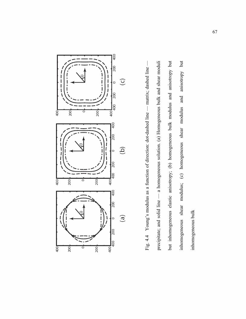
67

Fig.

4.4

Y

oung

’s m

odul

us a

s a

func

tion

of d

irect

ion:

dot

-das

hed

line

— m

atrix

; das

hed

line

—

prec

ipita

te; a

nd s

olid

line

— a

hom

ogen

eous

sol

utio

n. (

a) H

omog

eneo

us b

ulk

and

shea

r m

odul

i

but

inho

mog

eneo

us e

last

ic a

niso

tropy

; (b

) ho

mog

eneo

us b

ulk

mod

ulus

and

ani

sotro

py b

ut

inho

mog

eneo

us

shea

r m

odul

us;

(c)

hom

ogen

eous

sh

ear

mod

ulus

an

d an

isot

ropy

bu

t

inho

mog

eneo

us b

ulk

68


different degrees of elastic anisotropy in the matrix and precipitate ( Pδ , Mδ ): (a) (1.00,

1.00), (b) (1.14, 0.89), (c) (1.34, 0.79), (d) (1.63, 0.72), (e) (2.05, 0.66), (f) (2.80, 0.61).

Both the bulk and shear moduli are homogeneous.

69


different shear moduli in the two phases (a) β = 1.0, (b) β = 1.2, (c) β = 1.5, (d) β =

1.9, (e) β = 2.6, (f) β = 3.6. The precipitate and matrix have the same bulk moduli and

the same degree of elastic anisotropy.

70

Fig.

4.7

Tem

pora

l evo

lutio

n du

ring

phas

e se

para

tion

of a

hom

ogen

eous

sol

id s

olut

ion

into

a tw

o ph

ase

mix

ture

for t

he c

ase

of e

last

ic in

hom

ogen

eity

cau

sed

by d

iffer

ent s

hear

mod

uli i

n th

e tw

o ph

ases

, β =

2.6

.

The

prec

ipita

te a

nd m

atrix

hav

e th

e sa

me

bulk

mod

uli a

nd th

e sa

me

degr

ee o

f el

astic

ani

sotro

py.

71


different bulk moduli in the two phases (a) 0.1/ =MP BB , (b) 5.1/ =MP BB . The

precipitate and matrix have the same shear moduli and the same degree of elastic

anisotropy.

72

soft directions developed. With further coarsening, the initially interconnected hard phase

breaks into isolated particles. In the third case, the shear modulus and anisotropy are

independent of composition while the bulk modulus varies with composition. Fig. 4.4c

shows the Young’s moduli as a function of direction for the hard and soft phases. The

morphologies of a phase-separated two-phase system with different bulk modulus

inhomogeneity is shown in Fig. 4.8. It is found that the bulk modulus inhomogeneity has

essentially no important effect on the morphology. It should be emphasized although the

first-order approximations [37-39] predict the qualitatively correct two-phase

morphology, the local stress distributions described by a first-order approximation for a

system with strongly elastic inhomogeneity can be in serious error as shown in section

3.2.5. Therefore, the elastic energy contribution to the driving force for microstructure

evolution such as coarsening for two phase systems is not accurately determined in a first

order approximation, As a result, kinetics of microstructure evolutions and resulting

microstructures would be affected.

4.3 Spinodal decomposition in a film with periodically distributed interfacial dislocations

The translational symmetry in bulk materials is broken due to the presence of a

surface and an interface in a thin film on a substrate [162]. As a result, the kinetics of

phase transition in a film may differ dramatically from that in bulk materials. For

example, quasi-two dimensional diffusion may occur in a very thin film, and results in

the formation of cylindrical particles perpendicular to the surface during spinodal

decomposition. For a thick film, the stress relaxation at surface or stress gradient along

73

the film thickness causes an inhomogeneous decomposition rate and the development of

alternating layers of the phases lying parallel to the surface [42, 162-164]. Experiments

demonstrated that a regular network of pure edge-type dislocations with a spacing of

several nanometers could be formed directly at the heterointerface, which has extremely

large lattice mismatches between the film and substrate [165,167]. Like a surface, a

strained or patterned substrate breaks the translational symmetry in the film plane, which

can be used to control the wave length of spinodal decomposition and develop

nanostructures [162,168-172]. Romanov, et al [170] investigate the possibility of using

such dislocation arrays as to control the nucleation of self-assembled quantum dots.

Johnson, et. al [162,168,169] performed two-dimensional simulations of phase

decomposition in a film on a patterned substrate. Greaney, et al [172] studied the effect of

a rigid, periodically strained substrate on spinodal decomposition in a film. A linear

stability analysis [172] showed that a film will undergo spinodal decomposition with the

dominant wavelength determined by the periodicity of the substrate strain. The propose

of this section is to develop a three-dimensional (3D) phase field model for simulating the

spinodal decomposition in a film with periodically distributed interfacial dislocations or

lattice mismatches and subject to an elastically substrate constraint. The iteration method

described in section 3.3 is employed to solve the mechanical equilibrium equations in

thin films in the simultaneous presence of dislocations, compositional strains, and a

substrate constraint. In the thesis, only the results of spinodal decomposition in films with

a flat surface are presented. For the general case with a curve film surface, the formation

of self-assembled quantum dots due to surface instabilities is reported in our paper [136].

74

4.3.1 Phase-field model

Consider a cubic thin film grown heteroepitaxially on a cubic substrate at high

temperature and assume that a periodically dislocation array is formed at the interface

shown in Fig. 4.9. The Burgers vectors of dislocations are assumed to be along ]011[21

and ]011[21 , respectively. For simplicity, we assume the film is a binary solid solution,

which is unstable with respect to spinodal decomposition at the temperature of interest. In

the phase-field framework, the composition ),( tc x , which represents the mole or atom

fraction at position x and time t, is chosen as the phase variable. If we ignore the

microstructural evolution of the substrate and the dislocation core energy, then the total

energy of the system includes chemical free energy, gradient energy due to composition

inhomogeneity, and elastic energy,

xdttttctcfE klijijklv

322

)],(),(),(21)),((

2)),(([ xxxxx εελκ

+∇+= ∫ . (4.7)

where )),(( txcf is the chemical free energy density, κ is the gradient energy coefficient.

The third term in (4.7) is the elastic energy density. The chemical free energy density

(4.5) is employed. The elastic problem is described in the section 3.3, and is solved by the

iteration method [158].

75

4.3.2 Evolution equation

The kinetic equation of the composition is the same as the equation (4.2). In the

present work, we ignore the morphological instabilities in the film surface, and assume

the composition flux at the surface of the film and interface between the film and the

substrate are zero. Therefore, the temporal evolution of the composition field is obtained

by solving the equation (4.2) together with the initial conditions and the following

boundary conditions

0),(=

∂∂

−= fhzztxc and 0),(

0

=∂

∂

=zztxc (4.8)

To numerically solve this evolution equation, a Fourier-spectral method is used in x and y

directions. Since the zero-flux boundary conditions at film surface and film/substrate

interface cannot be satisfied by a Fourier expansion, a second-order finite difference

method with FFT (Fast Fourier Transform) is used in the z-direction. In time

discretization, a semi-implicit method is employed [159].

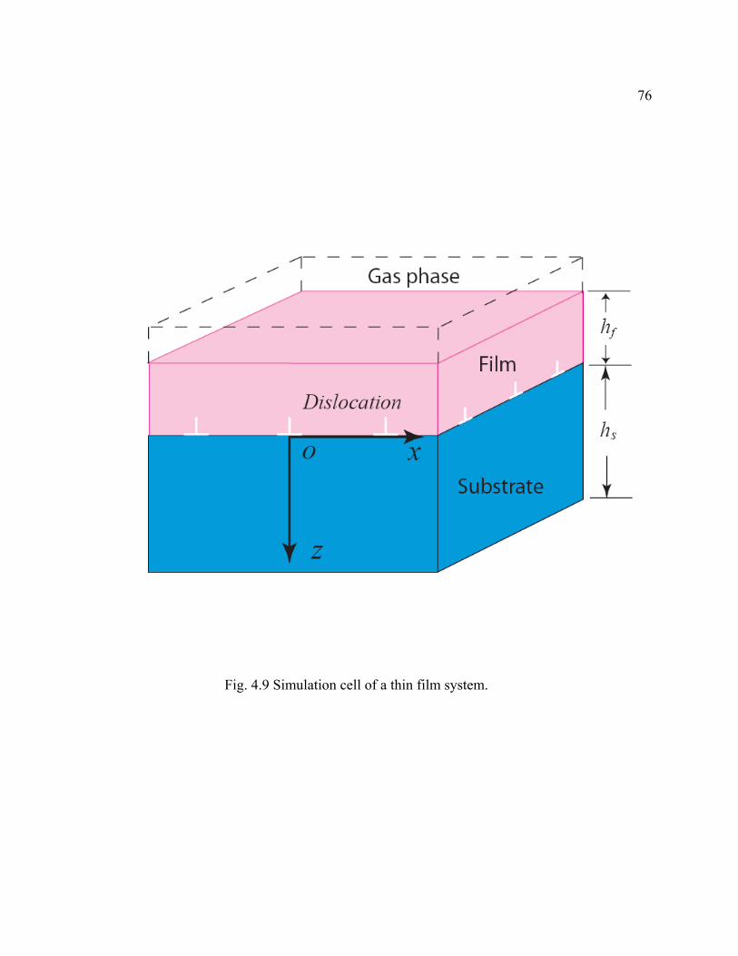
76

Fig. 4.9 Simulation cell of a thin film system.

77

4.3.3 Results and discussions

In the simulation, 32128128 ×× discrete grid points are used. The thickness of the

substrate is 18=sh . In order to study the effect of the film thickness on the

microstructure pattern, three different film thickness 3=fh , 5 and 9 are considered,

respectively. The dimensionless time *t∆ is chosen to be 0.05. The interfacial energy is

assumed to be isotropic, and the dimensionless gradient energy coefficient, 2*κ , is taken

to be 0.5. The overall reduced composition used in this study is 0.5. The isotropic elastic

constants are assumed for both film and substrate, 30011 =C , 10012 =C , 10044 =C , in

the unit of TkN BV where VN is the number of atoms per unit volume. Considering that

the linear elasticity theory is only valid outside the dislocation core region, the

characteristic length 0d is taken to be 10b about dislocation core size, where b is the

magnitude of the Burgers’ vector of the dislocation. In the present work, our main

concern is the effect of nonuniform lattice mismatches at the film/substrate interface on

morphological evolution during spinodal decomposition. Particularly, the nonuniform

interface lattice mismatches are related to a distribution of interfacial dislocations.

Assume nx edge dislocations and ny edge dislocations are uniformly distributed in x- and

y- directions, respectively. The nonzero components of the eigenstrain tensor related to

such a dislocation distribution can be described as

0)),5.0128(()()),5.0128(()(1

221

1121

<−−=−−= ∑∑==

zifny

ydb

nxx

db ny

n

disnx

n

dis δεδε00

rr (4.9)

78

First let us compare the composition evolution in two cases. In case I, the lattice

mismatch is uniform, 00165.02211 == disdis εε . And in case II, the total lattice mismatch is

the same as that in case I, but the uniform lattice mismatch is replaced by two

dislocations in both x- and y- directions. The thickness of the film is 03d . We start the

simulation with a very small composition fluctuation. Fig. 4.10 shows the snapshots of

composition evolution in the course of spinodal decomposition. The red color denotes

solute rich region while white color solvent rich region. It is clearly seen that two

interconnected phases gradually formed in case I. Since the film is very thin, and the

diffusion fluxes normal to the surface and the interface are assumed to zero, the diffusion

occurs on the plane parallel to the interface. As a result, each phase has a columnar

morphology perpendicular to the interface. Our previous results [42] show that as the film

thickness increases, the morphology of each phase becomes a 3D network similar to that

of bulk materials. For case II, the interaction between stress fields from interfacial

dislocations and compositional strains dominates the spinodal decomposition process and

causes a directional spinodal decomposition. Fig. 4.11 presents the morphological

evolution during spinodal decomposition in the film. To see more clearly the composition

wave evolution, Fig. 4.12 plots the temporal composition evolution along A-A line

shown in Fig. 4.11. It can be seen that at the initial stage the local stress results in the

formation of composition waves near the dislocation along the direction perpendicular to

the dislocation line on the film plane as well as along the thickness direction. The

composition wave along thickness is transient. As the time increases, such a composition

wave disappears. The composition wave along the direction perpendicular to the

79

dislocation line on the film plane propagates directionally as time increases. Finally, an

mesoscopically ordered microstructure is formed.

To illustrate the effect of the wavelength of dislocation distributions on the

microstructure pattern, four different dislocation distributions ( 2== nynx , 4, 8 and 16)

are simulated. Fig. 4.13 presents the microstructure patterns at simulation step 1000=t .

It can be seen that with the increase of the dislocation density or the decrease of the

wavelength, the morphology of two decomposed phases changes dramatically from

interconnected to isolated particles. The results demonstrate that a nanostructure can be

obtained by decreasing the wavelength of dislocation distributions. Fig. 4.14 illustrates

how the thickness of the film affects the microstructure patterns. The microstructures at

simulation step 1000=t are shown for three different simulations corresponding to three

different film thickness 3=fh , 5 and 9 for the case with 8 dislocations ( 8== nynx ).

The left figure presents the morphology of the solute rich phase. It is clearly seen that as

the thickness increases, the composition wave along the thickness direction starts to form.

With sufficient thickness, a microstructure with two alternating layers of the phases is

developed. In addition, the morphology of the phases in each layer is different from that

in the thin films ( 3=fh )

80


under a uniform substrate constraint.

81


with two interfacial dislocations in both x- and y- directions.

82

Fig. 4.12 Composition profile along A-A line shown in Fig.4.11 during spinodal

decomposition.

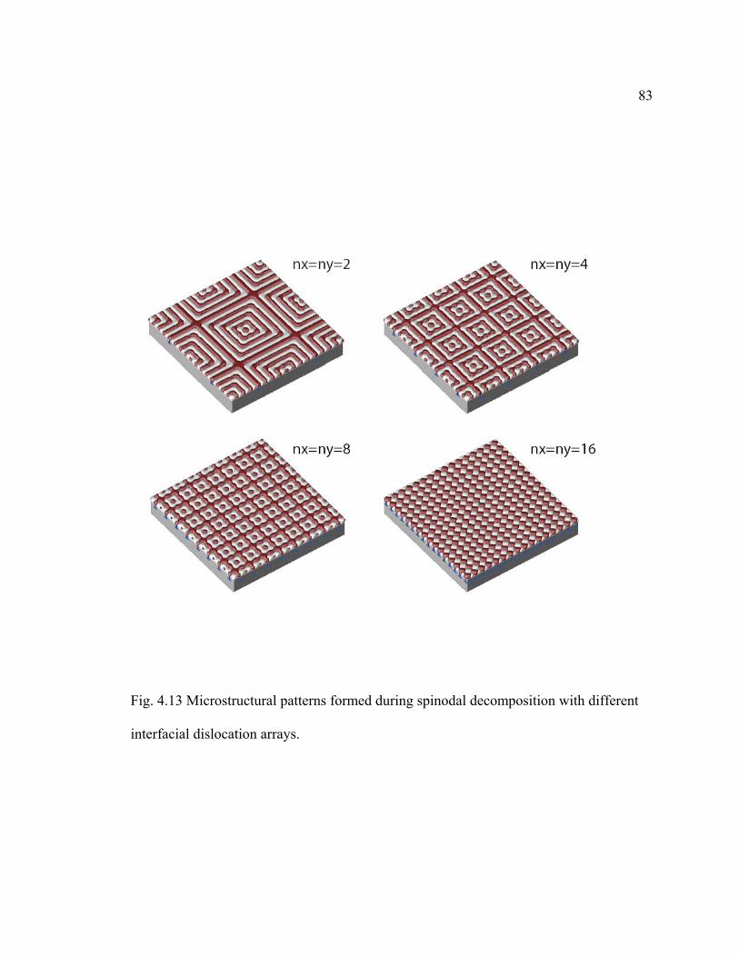
83

Fig. 4.13 Microstructural patterns formed during spinodal decomposition with different

interfacial dislocation arrays.

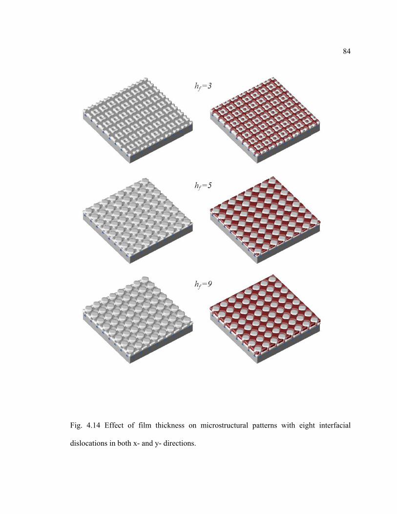
84

Fig. 4.14 Effect of film thickness on microstructural patterns with eight interfacial

dislocations in both x- and y- directions.

85

4.4 Conclusion

A phase-field model is developed to simulate the spinodal decomposition in a

solid with strongly elastic inhomogeneity and with a spatial distribution of dislocations.

The iteration method is used to calculate the elastic energy. As examples, the

morphological dependence of the separated phases on elastic inhomogeneity in 2D and

spinodal decomposition in a film with periodically distributed interfacial dislocations in

3D are studied. For a solid with cubic elastic anisotropy the equilibrium shape of an

isolated precipitate is studied as a function of the ratio of shear modulus in the precipitate

and the matrix. The results show that the hard connected phase becomes gradually

unconnected particles and the particles align along the softer directions 10 and 01 as

the inhomogeneity in shear modulus or elastic anisotropy increases. The inhomogeneity

of bulk modulus does not affect the morphology of separated phases. Simulation results

in films demonstrate that dislocation stresses induce a directional spinodal

decomposition. Periodically distributed interfacial dislocations can be used to create self-

assembled nanostructures. The nanostructure can be changed by varying the film

thickness and the wavelength of the interfacial dislocation distribution.

86

Chapter 5

A Phase-field Model of Dislocation Dynamics

To describe the phase-field model of dislocation dynamics, a binary alloy with

mobile dislocations and diffusive solutes is taken as a model system. Two sets of phase

field variables, i.e., compositional field ),( tc x and order parameter fields ),( txη , are

employed to describe the mole fraction of solutes and dislocation distribution at position

x and time t, respectively. If the single crystal of interest has N slip systems, N order

parameter fields ),( txαβη ( ∑ ==

p mN1α α , α =1,2,…, p ; 1=β ,2,…, αm ) are needed to

completely describe the dislocation distribution, where p denotes the number of

elementary slip planes and αm denotes the number of elementary Burgers vectors on the

slip plane α . For instance, in a FCC single crystal, there are four slip planes: (111),

( 111 ), (1 1 1), (11 1 ), and three slip directions on each slip plane, and hence it requires

12 order parameter fields ),( txαβη (p=4, and 3=αm ( 4,3,2,1=α ))

5.1 Total free energy of the system

The total free energy E in a binary system with dislocations includes (1) the

chemical free energy Echem which consists of both the local bulk free energy of a binary

solution and the composition gradient energy, (2) elastic energy Eelast associated with

solutes, defects and applied stresses, and (3) ‘crystalline energy’ Ecryst which includes the

local structural energy and the structural gradient energy. For a perfect dislocation, the

87

crystalline energy is exactly associated with the dislocation core energy. Therefore, the

total free energy of the system is described by

crystelastchem EEEE ++= (5.1)

5.1.1 Chemical free energy

In a binary system with a spatial composition distribution ),( tc x , the chemical

free energy can be described as the sum of two contributions, i.e., the local bulk free

energy and the gradient energy. It reads

dVccfEV

chem ∫ ∇+= ])(2

)([ 22

0κ (5.2)

where the first term )(0 cf is the bulk free energy density of a binary solution; the second

term is the gradient energy density, and κ is the gradient energy coefficient. For a

regular solution, )(0 cf has the form,

)]1ln()1()ln()1([)(0 ccccccRTcf −−++−= ϕ (5.3)

where R is the ideal gas constant, T is the absolute temperature, and ϕ is a material

constant. For an ideal solution, ϕ is equal to zero.

88


The elastic energy can be calculated by (see [1,139] for detail)

dVE elkl

elij

Vijkl

elast εελ∫=21 (5.4)

where

)(),()),(()( xxxx defij

disij

cijijij

elij ttc εεεδεεε −−−+= (5.5)

ijklλ is the elastic stiffness tensor, ijε the homogeneous macroscopic strain characterizing

the macroscopic shape and volume change, )(xijδε heterogeneous strains, )),(( tccij xε

the eigenstrain due to the composition inhomogeneity and )(xdefijε the eigenstrain

associated with immobile defects such as inclusions. The eigenstrain ),( tdisij xε is

associated with the dislocation distribution,

( ) ( ) ( ) ( ) ( ) ( ) ( )∑∑ =+

=βα

αβαββα

ααβααβ ηβαεηε,,

),(),(),(2

, tftfd

injbjnibt dis

ijo

disij xxx (5.6)

89

where ( )),( tf xη is the shape function which describes the change of Burgers vector

across the dislocation core. In the original phase-field model of dislocation dynamics

[87,88], ( )),( tf xη has assigned a linear function of ),( txη ,

),()),(( ttf xx ηη = (5.7)

It is found that such a shape function leads to a dependence of Burgers vector on applied

stress, hence, a wrong stress field of dislocations. In this thesis, a new shape function is

constructed which can eliminate the dependence of the magnitude of the dislocation

Burgers vector on the applied stress and provide a correct stress field of dislocations. The

new shape function has the following form [173]

( ) ( )),(2sin21),(),( tttf xxx πηπ

ηη −= (5.8)

The function )),(( tf xη has two properties: (i) it is exactly equal to ),( txη when ),( txη

is an integer; and (ii) its derivatives at integer values of ),( txη are zero.

5.1.3 ‘Crystalline energy’ associated with dislocations

As a microscopic interpretation, the order parameter ),( txαβη represents the

relative displacement between two atomic planes on the slip plane. Imitating the ‘Peierls

90

potential’ in a crystal and the gradient energy in phase field theory, Khachaturyan et al

[87,88] constructed a ‘Crystalline energy’ of dislocations

xdx

tbx

tbBtAEl

k

j

ip q

ijkl

p qcryst 321

1 121

2

1 1

),,(),,(),(2

)],([sin),(1 2

∂∂

∂∂

+= ∑∑∫ ∑∑= == =

xxx ααααγπηβα

α ααβ

α β

(5.9)

where γ is a positive constant, ),( βαA and ),( βαijklB are material constants that can be

obtained by fitting the core energy and core size of dislocations, and ),,( txb α is the total

Burgers vector of dislocations at x on slip plane α ,

∑=

=α

βαβαβηα

m

tt1

),(),,( xbxb (5.10)

In equation (5.9) the first term is the ‘Peierls potential’ (local structural energy), and the

second term is the structural gradient energy.

5.2 Phase-field kinetic equations

The temporal evolution of solute composition c is described by the Cahn-Hilliard

equation

),(),(

),( ttc

EMt

tc xx

x ξδδ

+∇=∂

∂ (5.11)

91

where E is the total free energy of the system, M is a kinetic coefficient related to the

solute diffusion mobility, and ),( txξ is the noise term reflecting the thermal fluctuation.

Substituting the total energy into the Cahn-Hilliard equation (5.11) and taking the first

variational derivatives with respect to the composition function ),( tc x . The composition

field kinetic equation is given by

[ ] ( )( )

( ) ( )ttcc

tcf

tf

tctMt

tc

defkl

disklijijkl

klijijklklklijijkl

,),(),(

)](),(),([

),(),(),(

20

,

0

2002

xxx

xx

xxx

ξκ

εηβαεδελ

δδελδεεδελ

αββα

+∇−∂

∂+

++

++−∇=∂

∂

∑ (5.12)

The order parameter fields describing the dislocation distribution are non-conserved, and

their temporal evolutions are described by the time-dependent Ginzburg-Landau

equations:

),,,(),(

),(t

tEL

tt

xx

xβαζ

δηδη

αβαβ

αβ +−=∂

∂ (5.13)

where αβL is the kinetic coefficient characterizing the dislocation mobility, and

),,,( txβαζ is the Langevin Gaussian noise term simulating the thermal fluctuations.

Equation (5.13) can be rewritten as

92

( )

( )

( ) ),,,(),(2

),(2sin

)](),(),(),(

),([),(

),(),(

,

0

tttA

tftc

ttf

Lt

t

defkl

disklkl

klkldisijijkl

xxx

xxx

xxx

βαζηφγπηπ

εηβαεδε

δεεη

ηβαελ

η

αβαβ

αββα

αβ

αβαβ

αβ

+∂∂

−−

−−−

+∂

∂=

∂

∂

∑ (5.14)

where ),( βαAA = is assumed to be constant in the simulation for simplicity, and

∑ ∑= = ∂∂

∂∂

=p p

l

k

j

iijkl x

tbx

tbBt

1 121

211 2

]),,(),,(

),([),(α α

ααααφ

xxx (5.15)

To facilitate the computation, the following dimensionless parameters are introduced,

20

*20

elas*elas

20

0*0

20

20

*20

*

20

*20

20

*20

*

0

ij*ij

0

ij*ij

ijkl*ijkl

0

00

0

*

0

*

GεRTχ ,

GεEE ,

Gε(c)f

(c)f

εGdκκ ,

LdMM

tLGεt ,ε2Gd

γγ ,Gε

AA

Gεσ

σ,εε

ε ,Gλ

λ

da

ε,d

xd,d

===

==

===

===

=∆

==xx

(5.16)

where G is the shear modulus, and x∆ is the grid spacing of the computational mesh.

93

The elastic equilibrium equation and the kinetic equations are solved numerically.

The semi-implicit spectral method [159] is employed, which implies the use of periodic

boundary conditions along x-, y- and z-directions ( xx =1 , yx =2 , zx =3 ). In all the

simulations, the following parameters are fixed: 0.311 =C , 0.112 =C , 0.144 =C ,

05.0* =A , 25.0* =γ , 05.0* =κ , 075.00 =ε , 09.0* =χ , 25.00 =ε , 02.0* =dt ;

0.1* =d , 00 4ad = where 0a is the length of Burgers vector. The dimensionless

parameters *M , ϕ , 0c and *ijε are systematically changed to study their effect on

dislocation-solute interactions under applied stresses. In the simulations, elastic

inhomogeneity and immobile defects are not considered. But it is straightforward to

incorporate these effects into the phase-field model of dislocation dynamics with the

iteration method developed above.

5.3 Results and discussions

5.3.1 Stress fields of dislocations

Eigenstrain of dislocations is described by equation (5.6). Different shape

functions )),(( txf η might affect the dislocation stress field. To examine the dislocation

stress field, a two-dimensional simulation cell with a dislocation loop shown in Fig. 5.1 is

considered because an analytical elastic solution exists in this case. We assume that the

composition of solutes is zero. The dislocation loop with xR ∆= 120 is introduced into

the center of the simulation cell 512512× by assigning the initial value 1=η on the grid

94

Fig. 5.1 Schematic illustration of a dislocation loop located at the center of a 2D

computational cell.

95

points inside the dislocation loop on the slip plane and 0=η outside the loop. The

Burgers vector of the dislocation loop is b=(100) along the x- direction, and its slip plane

is the n=(001) plane. The equilibrium profile )(0 xη of kinetic equation (5.14) in the

absence of applied stresses is used to calculate the stress field of the dislocation. Fig. 5.2

plots the normal and shear stress distributions of the edge dislocation in the right side of

simulation cell along A-A line just below the slip plane shown in Fig. 5.1. The

corresponding analytical solution is also plotted for comparison. The results show that the

stress fields obtained with the new expression of dislocation eigenstrains (5.8) are in good

agreement with the analytical elastic solution except for two or three points where the

stresses of analytical solutions are singular. In addition, it is found that numerical stresses

are continuous at the dislocation line. This means that the singularity of the stress field at

the dislocation line is removed. It is a natural result since the discontinuous displacement

at a dislocation line in classical elastic theory is replaced by a continuous displacement in

the phase field model. Therefore, phase-field models of dislocations provide similar

elastic stress fields as the non-local elastic theory [108,109]. The elimination of

singularity not only brings the dislocation stress field much closer to the real situation but

also benefits the stability of numerical calculations.

For a static dislocation, the linear expression (5.7) is able to provide a correct

stress field. However, it results in the dependence of the magnitude of the dislocation

Burgers vector on applied stresses, hence, an incorrect stress field for a moving

dislocation. To examine the effect of two dislocation eigenstrain expressions on the stress

96

field of moving dislocations, the kinetic equation (5.14) is solved under different applied

shear stresses *31σ . Fig. 5.3 shows the temporal order parameter profiles at ** 400dtt = ,

*800dt , ,1200 *dt and *1600dt with a loading history *31σ = 0.0, 0.015, 0.02 and 0.025 for

every 400 time steps. The related shear stress distributions on the slip plane are plotted in

Fig. 5.4. It is observed in Fig. 5.3b that the order parameter values inside and outside the

dislocation loop increase with the magnitude of the applied stress for the case that the

dislocation eigenstrain expression is a linear function of the order parameter in equation

(5.7). This implies that dislocation Burgers vector depends on the applied stress. From

Fig. 5.4b, it can be seen that an extra stress field due to the change of Burgers vector

greatly reduces the effect of the applied stress. As a result, the extra stress slows down the

dislocation velocity. However, the new eigenstrain expression (5.8) proposed in the

present thesis eliminates this dependence. The order parameter profiles in Fig. 5.3a show

that the order parameter values far away from the dislocation core do not change under

applied stresses with the new eigenstrain expression. The applied stresses and internal

stresses affect only the order parameter profile in the dislocation core. Therefore, the

dislocation stress field far away from the dislocation core remains the same during

dislocation motion under different applied stresses, which can be seen from Fig. 5.4a.

These results demonstrate that the new dislocation eigenstrain expression can provide a

correct stress field for both static and moving dislocations. It should be pointed out that

the internal stress fields produced by other crystal defects such as other dislocations and

cracks will also lead to a change in the Burgers vector if the linear eigenstrain expression

is employed. Such a dependency is eliminated using the new eigenstrain expression.

97

Fig. 5.2 Comparison of dislocation stress distributions calculated from numerical and

analytical solutions along A-A line shown in Fig. 5.1, the solid lines for analytical

solution and the symbol lines for numerical solutions.

98

Fig. 5.3a Order parameter profiles under different applied stresses *31σ with a nonlinear

dependence of the dislocation eigenstrain on order parameter.

99

Fig. 5.3b Order parameter profiles under different applied stresses *31σ with the linear

expression of the dislocation eigenstrain on order parameter.

100

Fig. 5.4a Shear stress distributions along the slip plane for a moving dislocation with the

non-linear eigenstrain expression.

101

Fig. 5.4b Shear stress distributions along the slip plane for a moving dislocation with

the new dislocation eigenstrain expression.

102

5.3.2 Phase-plane analysis of dislocation velocity

The coefficient αβL in the evolution equation (5.14) is unknown, which is the

kinetic coefficient characterizing the dislocation mobility. A relationship among the

coefficient αβL , the dislocation velocity and applied stresses can be established through

the phase-plane analysis [174]. With such a relationship, experimental data about the

dislocation velocity versus applied stress can be used to determine the coefficient αβL .

To do the phase plane analysis, consider a single dislocation located in the center

of the simulation cell shown in Fig. 5.1. The evolution equation of dislocation (5.14)

becomes

])(2)2sin([ 3131 ηηεσπηπγηη

∂∂

+−=fAL dis

xxt (5.17)

with boundary conditions:

βηαη =∞=−∞ ),(,),( tt (5.18)

where 31σ is the total stress component included the dislocation self-stress and the

applied stress. The subscript of η means its partial derivative, for instance, tt ∂

∂=

ηη ,

103

2

2

xxx ∂∂

=ηη . α and β , which depend on the form of function )(ηf , are the roots of the

following equation when ±∞→x , respectively,

0)(2)2sin( 3131 =∂∂

+−ηηεσπηπ fA dis (5.19)

Because the dislocation self-stress field is zero as ±∞→x , .2 310313131 constdisdis == εσεσ

031σ is the applied stress. If ηη =)(f , the equation becomes

02)2sin( 31031 =+− disA εσπηπ (5.20)

It is found that the equilibrium values, α and β , depend on applied stress. However, for

the new shape function (5.8), the equation reads

0)2sin( =− πηπA (5.21)

The equilibrium values, 1=α and 0=β , are independent of the applied stress.

Therefore, the same conclusion, the new shape function can eliminate the dependence of

Burgers vector on the applied stress, can be obtained from the analysis of equilibrium

properties of the solution for the order parameter variable.

104

In the derivation of dislocation velocity under applied shear stress 031σ with phase-plane

analysis, the new shape function ππηηη

2)2sin()( −=f is employed. The equation (5.17)

in a dimensionless form is written as

))2cos(1()(2)2sin(2 *31

*31

*031

*** πηεσσπηπηγη ζζ −++−= disdis

tA (5.22)

with boundary conditions

0),(,1),( ** =∞=−∞ tt ηη (5.23)

where *31disσ is the self-stress of the dislocation.

Assume equation (5.23) has a traveling wave )( *xη solution and the velocity is

v . In the moving coordinate ** vtx −=ζ , equation (5.22) is rewritten as

))2cos(1()(2)2sin(2 *31

*31

*031

** πηεσσπηπηγη ζζζ −++−=− disdisAv (5.24)

with the boundary conditions

0)(,1)( =∞=−∞ ηη (5.25)

105

Introduce a function φ and let ζηφ = , equation (5.24) becomes

))2cos(1()(2)2sin(2 *31

*31

*031

** πηεσσπηπφφγ ζ −+−+−= disdisAv (5.26)

with the boundary conditions

0)(,0)( =∞=−∞ φφ (5.27)

Multiply both sides of equation (5.26) with φ and integrate from ),( ∞−∞

ζπηεσσφπφπφφζφφγ ζ dAvd disdis ))]2cos(1()(2)2sin([2 *31

*31

*031

*2* −+−−−= ∫∫∞

∞−

∞

∞−

(5.28)

the velocity is given by

∫

∫ −+−= 1

0

1

0

*31

*31

*031 ))2cos(1()(2

ηφ

ηπηεσσ

d

dv

disdis

(5.29)

Since the stress component *31disσ is asymmetric, it becomes

106

∫−= 1

0

*031

*0312

ηφ

εσ

dv

dis

(5.30)

where φ is the solution of equation (5.26) under applied stresses. As a first order

approximation, assume that φ is independent of applied stress when applied stress is

small. Therefore, it can be seen that there exists a linear relationship between dislocation

velocity v and applied stress 031σ .

5.3.3 Dislocation velocity and discretization effect

To examine numerically the relationship between the velocity of a dislocation and

the applied stress, the motion of dislocations in two dimensions shown in Fig. 5.1 is

simulated under different applied stresses. The velocities (the displacement of the

dislocation within a fixed number of time steps) are calculated. Fig. 5.5a shows the

velocity of the dislocation as a function of applied stresses and grid sizes for eigenstrain

expressions (5.8). There are three observations. First, the dislocation velocity strongly

depends on the grid size (i.e., discretization effect). It increases as the grid size decreases

for a given applied stress. However, the velocity is convergent when the grid size *d is

less than 0.1 . Second, a linear relationship between the dislocation velocity and the

applied stress exists for the convergent cases. From the phase-plane analysis discussed in

the last section, the dislocation velocity can be calculated with

107

Fig. 5.5a Average velocity of a dislocation vs applied shear stress shows the effect of

discretization.

108

Fig. 5.5b Average velocity of a dislocation vs applied shear stress shows the effect of

different eigenstrain expressions.

109

*031

*1

0

*031

*0312 σ

ηφ

εσ Sd

vdis

=−=

∫ (5.31)

The value )/(3.5 *0

* tdS = calculated is in good agreement with the numerical result

)/(1.5 *0

* tdS = for the convergent cases. Finally, the fact, that the velocity tends to zero

as the applied stress tends to zero, implies that no critical stress exists for moving an

isolated dislocation. In other words, Peierls stress is not taken into account in this phase

field model although the total energy includes the term ‘Peierls potential’. Any critical

stress appearing in the cases with larger grid sizes comes from discretization effect. For a

comparison, the same simulations are performed by using eigenstrain expressions (5.7).

Similar discretization effect is observed. From Fig. 5.5b, it can be found that the velocity

obtained by using eigenstrain expressions (5.7) is much smaller than that obtained by

using eigenstrain expressions (5.8) under the same applied stress. This is consistent with

the discussion in section 5.3 that part of the work done by the applied stress is spent on

increasing the Burgers vector of the dislocation for the case of eigenstrain expression

(5.7), and hence the corresponding dislocation velocity is reduced.

5.3.4 Average velocity of dislocations

The dynamic interaction between moving dislocation and diffusive solutes will

affect the response of dislocations to applied stress, hence, the average velocity of

dislocations. Fig. 5.6 presents the average velocity of a dislocation during 1200

simulation steps as a function of the ratio *M of solute mobility to dislocation mobility,

110

overall composition 0c and applied stress. It is quite apparent from the results shown in

Fig. 5.6a that average velocity decreases with the increase in overall composition 0c for a

given *M and applied stress *031σ . The reason is the fact that higher overall solute

composition causes more solute segregation near a moving dislocation, hence larger

dragging stress. Three characteristic velocities of dislocations can be observed from Fig.

5.6a-b for any given overall solute composition and applied stress. One extreme case is

that *M tends to zero. This implies that solute diffusion becomes very slow compared to

dislocation motion. As a result, solute segregation mainly occurs in the dislocation core

region where a high driving force exists due to the large stress gradient. The dislocation

velocity reaches maximum which is almost independent of the overall compositions, but

depends on the magnitude of the applied stress.

Another extreme case is the instantaneous establishment of equilibrium solute

segregation profile around a dislocation, i.e. solutes diffuse much faster than the

dislocation motion when *M becomes very large. The average dragging stress exerted on

the dislocations by the solutes decreases, and tends to a constant. Such a constant

dragging stress depends on the equilibrium solute segregation affected by the overall

solute composition and the dislocation velocity or applied stresses. As a result,

dislocation velocity increases and becomes a constant. Finally, it is shown that there

exists a certain ratio *M of solute diffusion mobility to dislocation mobility that leads to

the minimum in dislocation velocity. From the results it can be found that such a *M is

independent of solute overall

111

Fig. 5.6a Average velocity of a dislocation as a function of 0* / LdMM = for different

overall compositions under an applied stress 04.0*31 =σ .

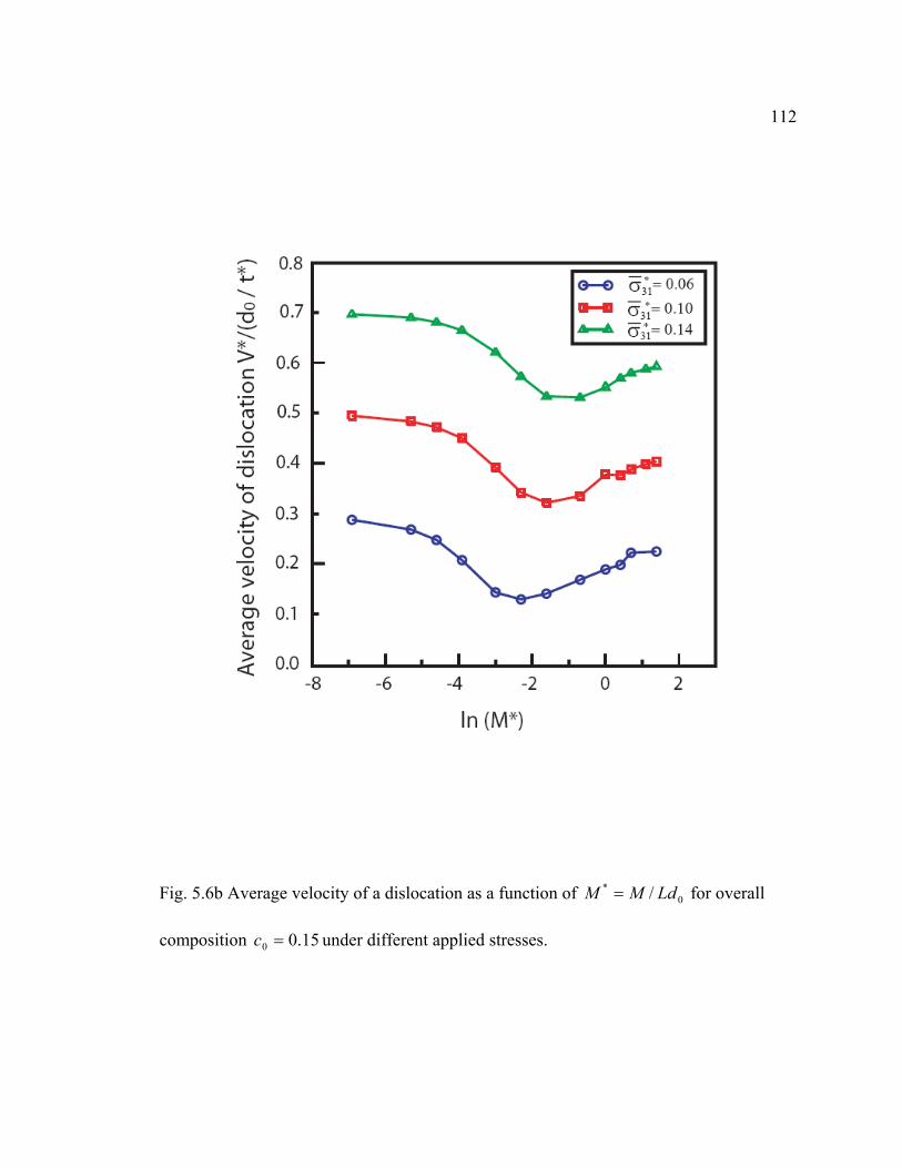
112

Fig. 5.6b Average velocity of a dislocation as a function of 0* / LdMM = for overall

composition 15.00 =c under different applied stresses.

113

composition but increases with the increase in applied stresses. The solute atmosphere

and dragging stress at such a critical situation will be analyzed in the following sections.

5.3.5 Solute atmosphere

For a given overall solute composition 15.00 =c and applied stress 04.0*031 =σ ,

three characteristic profiles of solute atmospheres around a moving dislocation are shown

in Fig. 5.7a-c. As expected, *M dramatically affects the size, shape and composition

profile of solute atmospheres. It is important to notice the position of the dislocation with

respect to the solute atmosphere. Comparing the solute atmospheres and average

velocities for the two cases in Fig. 5.7b-c, we find that it is not necessarily true that

higher segregation causes larger dragging stress. *M affects not only the solute

atmosphere profile but also the relative position of the profile with respect to the

dislocation, and thus the dragging stress. For the case of 5.0* =M under different

applied stresses 06.0*031 =σ , 0.1 and 0.14, steady-state solute atmospheres form around

moving dislocations. Fig. 5.7d-f show the steady-state atmospheres. We can see that the

size of atmosphere region decreases with the increase in applied stress.

5.3.6 Portevin-Le Chatelier effect and dynamic dragging stresses

Portevin-Le Chartelier (PLC) effect in solid solutions is related to the dynamic

interaction between diffusing solute atoms and mobile dislocations, i.e., an alternating

114

Fig. 5.7 Solute atmosphere around a moving dislocation in a solid solution with overall

composition 15.00 =c . (a), (b) and (c) were obtained under applied stress 04.0*31 =σ and

with =*M 0.005, 0.2 and 3.0 respectively; (d), (e) and (f) were obtained with 5.0* =M

under different applied stresses 0.06, 0.1 and 0.14, respectively.

115

Fig. 5.8a Dislocation velocity under applied stress 1.0*31 =σ .

116

Fig. 5.8b Dynamic dragging stress of solute atmosphere under applied stress 1.0*31 =σ .

117

process of the formation of solute atmosphere at dislocations and the unlocking of

dislocations from their solute atmospheres. The Portevin-Le Chatelier effect [175-179] is

characterized by a number of experimental observations such as the upper yield point,

serration in the tensile stress vs strain curves, and abnormal yield stress which increases

and then decreases as temperature increases. The average dislocation velocity as a

function of time presented in section 5.6 exhibits similar phenomenon to the macroscopic

Portevin-Le Chatelier effect. *M is the ratio of solute mobility to dislocation mobility.

Dislocation mobility depends on the atomistic structure of the dislocation core. If we

assume that the dislocation mobility is constant, Fig. 5.6 shows a relation between

average dislocation velocity and solute mobility. For substitutional solutes, its mobility

strongly depends on temperature. Solute mobility increases as temperature increases.

Therefore, the −x axes in Fig. 5.6 can be viewed as temperature axes. All results in Fig.

5.6 demonstrate a common tendency, i.e., the average dislocation velocity decreases and

then increases as temperature increases. Such a dependence of dislocation velocity

implies that the macroscopic yield stress increases and then decreases with an increase in

temperature, i.e. the Portevin-Le Chatelier effect.

The origin of Portevin-Le Chatelier effect in solute solution is the dynamic

interaction between diffusing solute atoms and mobile dislocations. In order to examine

the dynamic interaction, temporal dislocation velocities and dynamic dragging stress of

solute atmospheres are calculated for the cases shown in Fig. 5.7a-c in which the

dislocation has the characteristic velocities. Temporal dislocation velocity versus the

distance of dislocation motion is plotted in Fig. 5.8a. A number of observations can be

118

made from the results. First, the formation of solute atmosphere slows down the

dislocation velocity to the characteristic average velocity. For example, the velocity

decreases from 0.45 to 0.29( *0 / td ) after dislocation moves about 010~5 d distance for

the case of 2.0* =M . Since in our simulation we assume there is no solute segregation

around the dislocation at 0* =t , the initial velocity should be the same at 0.45 for

different *M . Secondly, the dynamic interaction between the moving dislocation and its

solute atmosphere, which results in a temporal composition change at the dislocation

core, causes a periodic variation of dislocation velocity. It is found that the strength of

dynamic dragging corresponding to the amplitude of velocity oscillation is almost

independent of *M . However, the frequency of dislocation velocity oscillation depends

on *M . Finally, it is interesting to find that the average dislocation velocity decreases as

the frequency of dislocation velocity oscillation increases.

In continuum mechanics, the dragging stress of the solute atmosphere is defined

as the stress at the dislocation line. Fig. 5.8b presents the dragging stress of solute

atmosphere at dislocation line ( 5.0=η ) during the dislocation motion for the three cases

in Fig. 5.7a-c. As expected, the dragging stress changes periodically during the

dislocation motion, and the change frequency of the dragging stress is consistent with that

of the dislocation velocity. In our phase field model, the dislocation core is spread out

within the glide plane. Therefore, the stress at the dislocation line ( 5.0=η ) is not exactly

the total dragging stress of the solute atmosphere. However, it is found that the average

119

value of the dragging stress during a periodic variety of the dislocation velocity might

reflect a total dragging stress.

5.4 Conclusion

A phase field model is developed for modeling the dynamic interaction between

moving dislocations and diffusive solutes. Both the chemical potential of solid solution

and elastic interaction among solutes and dislocations are taken into consideration. A new

shape function is constructed which can eliminate the dependence of Burgers vector on

applied stress in the pervious phase field model of dislocation dynamics. A relationship

among dislocation mobility coefficient, applied stress and dislocation velocity is

established which can be used to determine the dislocation mobility coefficient for

quantitative simulation. The simulation results using a single dislocation in a two-

dimensional model system demonstrate that the model is able to describe correctly the

dynamic interaction between diffusive solutes and moving dislocation. The dynamic

dragging stress, average velocity of dislocation and solute flow around a moving

dislocation can be obtained. It is shown that the dynamic interaction between solutes and

dislocation results in the Portevin-Le Chatelier phenomena under certain ratios of solute

mobility to dislocation velocity. It is straightforward to extend this model to alloy system

with elastic inhomogeneity and arbitrary spatial defects.

120

Chapter 6

Quantitative Simulations of 'θ Precipitation in Al-Cu Alloys

The low density combined with high strength has made aluminum alloys one of

the primary materials used for automobile and aircraft applications, where higher

strength-to-weight ratio is a major design consideration. The significant contribution to

the high strength of heat-treatable aluminum alloys is due to fine spatial distributed

precipitates formed from a supersaturated solid solution that will act as obstacles to

moving dislocations. Composition, heat treatment and manufacturing technology all

affect the precipitation reactions, hence, the microstructures and the strengthening

response. Understanding well, especially in a quantitative manner, how these controlling

factors exert their influences on microstructures is central for developing advanced

aluminum alloys that could achieve the progressively desired level of performance.

Al-Cu alloys with copper contents of around 3 ~ 4.5 wt% Cu form the basis of an

important class of heat treatable aluminium alloys. It is a system with multi-stage

precipitation reactions involving transitional metastable phases which include Al solid

solution phase (α phase with a disordered fcc structure), metastable phases GPI, GPII

(also known as ''θ phase) and θ’-Al2Cu, and thermodynamic stable θ -Al2Cu phase. Fig.

6.1 presents the Al-Cu phase diagram in terms of temperature (F) and Cu composition

(wt%) at the Al-rich portion that is constructed from thermodynamic calculations [180].

121

Fig. 6.1 Al rich portion of the Al-Cu phase diagram.

122

The full precipitation sequence in a binary Al-Cu alloy is [181-182]: Solid

solution → GPI → GPII → θ’ → θ. However, for a given alloy system, a number of

experimental conditions such as the quenching rate, aging temperature and applied

stresses affect the real precipitation sequence. For example, around 150 ~ 190Co the

precipitation sequence starts with the appearance of GP zones, while the sequence begins

directly with θ’ precipitates if the aging temperature is higher than 190oC. The metastable

θ’ (Al2Cu) precipitates are one of the primary strengthening precipitates in Al-Cu alloys.

There are extensive experimental investigations about the atomistic structures and

morphologies of different phases in Al-Cu alloys [183-189]. However, little is known

about the effect of interfacial energy anisotropy, interfacial mobility anisotropy, coherent

or semi-coherent stress field and applied stressed on the morphology of θ’ precipitates

[190].

In this chapter, a quantitative phase-field model is developed for simulating 'θ

(Al2Cu) precipitation process in Al-Cu alloys using thermodynamic and kinetic data and

the material properties as input. The effect of interfacial energy anisotropy, interfacial

mobility anisotropy, coherent /or semi-coherent stress field and applied stressed on

growth behavior and morphology of theta prime precipitates are systematically studied.

123

6.1 Review of experimental facts

6.1.1 Crystal structures

The structures of GP zones, θ and θ’ phases have been identified [181, 183-189].

Fig. 6.2 presents the crystal structures of stable and metastable phases observed during

precipitation in Al-Cu alloys. Generally, GPI is considered to be a monolayer of copper

along 1 0 0 planes, while GPII (also called as ''θ ) consists of two or more 100 layers

of copper atoms separated by three layers of Al [189-191]. Both GPI and GPII are

coherent with the matrix. Although GPI structure is commonly accepted, there are

different opinions on the GPII structure. For example, other possible GPII structure

proposed by Guinier is a periodic arrangement of one layer of Al and 3 Cu-rich layers.

Some people consider GPII just to be a coarsened form of GPI [192]. But some people

consider GPII a separate ordered phase based on the discontinuity observed in the

hardness curves. First-principle calculation shows that the GPII structure is energetically

favorable [193], however, kinetic Monte Carlo method fails to prove the prediction of

First-principle calculation.

The 'θ -Al2Cu phase is a metastable precipitate. It has a tetragonal structure with

an orientation relationship matrix)100(||)100( 'θ . Experimental results demonstrate that

'θ precipitate is partially coherent [93,94], and its shape is plate-like [94,97,194]. The

broad face of a plate-like 'θ precipitate is coherent while the interface is semicoherent

around the rim of the plates. The orientation relationship matrix)100(||)100( 'θ and the

tetragonal crystal structure imply that there are three orientational variants of 'θ

124

precipitates with their c-axes parallel to the three cubic axes of the fcc matrix. Fig. 6.3 is

a transmission electron micrograph obtained from an Al-1.7at% Cu alloy aged to peak

hardness at 190oC for 30 hours. The morphologies of two 'θ precipitate variants, which

are edge-on, are clearly observed in Fig. 6.3 because the thin foil is viewed along a

matrix001 direction. Experimental results also show that the maximum hardness is

always associated with the presence of 'θ precipitates in the microstructure [195,196].

Therefore, 'θ precipitates are considered as one of the most favorable strengthening

precipitates in Al-Cu alloys. In the present work, we focus on simulating the precipitation

of 'θ precipitates.

θ -Al2Cu phase has a tetragonal structure (see Fig. 6.2). It is thermodynamically

stable phase, but kinetically unfavorable for direct precipitation from the solid solution,

especially at temperatures below 2500C. The large difference of lattice constants between

θ -Al2Cu phase and the matrix (see Fig. 6.2) results in a large interfacial energy and

elastic energy, leading to a large nucleation barrier. Therefore, to overcome this kinetic

barrier, the precipitation reaction of the equilibrium θ -Al2Cu phase often proceeds

through metastable transition phases that gradually change in structure from fcc to

tetragonal. As a result, the precipitates gradually lose coherency in the precipitation

reaction. Therefore, θ -Al2Cu precipitates are incoherent and have irregular-shape. To

maximize the strength of Al-Cu alloys, its formation is undesirable because incoherent

precipitates often reduce the strength of alloys.

125

Fig. 6.2 Crystal structure of the stable and metastable phases observed during

precipitation in Al-Cu alloys (reconstructed from Hornbogen [93] ).

126

Fig. 6.3 Transimission electron microgragh associated with the maximum peak of

hardness in an Al-1.7at%Cu alloy aged at 190oC for 30 hours. The foils were oriented

along matrix

001 . (from Ringer et al [197]).

127

6.1.2 Stress-free strain of θ’ phase

Fig. 6.4 shows a schematic graph of a plate-like 'θ precipitate in the matrix.

According to the orientation relationship between 'θ and the matrix and lattice constants

of 'θ and the matrix, the stress-free strains can be calculated by

−=

−==

α

αθ

α

αθ

ε

εε

nanamca

aa

z

yx

'*

'**

(6.1)

where 'θa , 'θc and αa are lattice constants of 'θ and the matrix, respectively. m and n are

the numbers of unit cells in 'θ and the matrix sides, i.e., m 'θ unit cells align with n unit

cells of fcc matrix across the interface around the rim of the plate-like precipitate. Based

on first-principle calculations at 0K [95], the stress free lattice constants of fcc solid

solution and 'θ are

nmcnmanma 5684.0,4019.0,3989.0 '' === θθα (6.2)

The stress-free strains are 00746.0** == yx εε which are independent of m and n.

Substituting the above lattice constants with different interface configuration m:n into

equation (6.2), Table 6.1 lists the stress-free strain *zε vs m:n. It can be clearly seen that

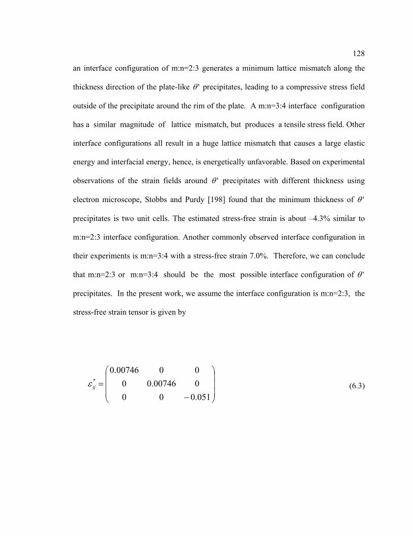
128

an interface configuration of m:n=2:3 generates a minimum lattice mismatch along the

thickness direction of the plate-like 'θ precipitates, leading to a compressive stress field

outside of the precipitate around the rim of the plate. A m:n=3:4 interface configuration

has a similar magnitude of lattice mismatch, but produces a tensile stress field. Other

interface configurations all result in a huge lattice mismatch that causes a large elastic

energy and interfacial energy, hence, is energetically unfavorable. Based on experimental

observations of the strain fields around 'θ precipitates with different thickness using

electron microscope, Stobbs and Purdy [198] found that the minimum thickness of 'θ

precipitates is two unit cells. The estimated stress-free strain is about –4.3% similar to

m:n=2:3 interface configuration. Another commonly observed interface configuration in

their experiments is m:n=3:4 with a stress-free strain 7.0%. Therefore, we can conclude

that m:n=2:3 or m:n=3:4 should be the most possible interface configuration of 'θ

precipitates. In the present work, we assume the interface configuration is m:n=2:3, the

stress-free strain tensor is given by

−=

051.000000746.000000746.0

*ijε (6.3)

129

Table 6.1 Stress-free strain zε in terms of interface configuration m:n

n

m 1 2 3 4 5

1 41.4% -29.3%

2 41.4% -5.1% -29.3%

3 41.4% 6.9% -14.5%

4 41.4% 41.4%

5 41.4%

130

(a)

Fig. 6.4 (a) orientation relationship of a plate-like 'θ precipitate, (b) two different

interface configurations around the rim of the plate where the interface is incoherent.

(b)

131

6.1.3 Nucleation of θ’ precipitates

There are varying views concerning the nucleation or formation of 'θ . Hardy and

Heal [199] found that the formation of 'θ stems from a rearrangement of atoms within a

high Cu concentration zone in the solid solution. This occurs by a gradual evolution of

the crystal structure rather than by nucleating a new phase by forming an embryo.

Another view considers that 'θ precipitates nucleate heterogeneously at the ''θ /Al matrix

interface or at defects such as dislocations. There are some experimental evidences that

'θ precipitate nucleates around dislocations [200,201]. It is also observed that small

amount of cold work prior to artificial aging enhances age hardening in a number of Al-

Cu-Mg alloys because of the introduction of dislocations that act as preferential

nucleation sites [202-208]. These results suggest that nucleation is independent of GP

zones or ''θ , and the initial distribution of 'θ is highly heterogeneous which reflects the

initial dislocation density in a particular grain. In addition, an analysis of the lattice

mismatch between 'θ and the matrix shows that 'θ preferentially nucleates on a/2<110>

dislocations, which can relieve the lattice mismatch in the <100> matrix directions. From

an estimate of the elastic interaction between coherent stresses associated with the lattice

mismatch and dislocation stress, two possible locations of 'θ nucleation are

schematically drawn in Fig. 6.5.

Like defect stresses, an applied stress also affects the nucleation of precipitates. Li [209]

first explained the phenomenon using the classical nucleation theory in which external

work by the applied stress compensates the strain energy associated with the lattice misfit

132

of the coherent precipitate nuclei. Tanaka et al. [210] employed a chemical reaction rate

approach [211,212] in which the applied stress effect was incorporated as a change in the

binding energy due to elastic interactions among solute atoms. They found that a very

small perturbation imposed on the binding energy corresponding to the stress effect might

change the nucleation rate drastically, which was in agreement with their experimental

observation in Fe–N single crystals. A directional applied stress might lead to preferred

directional nucleation and the precipitate alignment. Hosford and Agrawal’s results for

Al–3.98Cu aged at 210°C [213] show that the stress-orienting effect occurred during both

nucleation and growth stages of the θ’-precipitates but was more effective during the

nucleation stage which agrees with a recent phase-field simulation [105]. Using a two-

step (low-temperature+ high-temperature) aging procedure Eto et al’s observation [214]

demonstrated that the stress-orienting effect was initiated and determined during the

nucleation stage. The particular variant(s) of Guinier Preston (GP) zones was/were

preferentially formed under the directional stress and the aligned GP zones grew to θ’

plates through GP[II]. Sankaran’s explanation [215] took into account the preferred

nucleation on the stress-oriented dislocation structures.

In the present work, we ignore the nucleation process that involves atomistic

scale events. Therefore, in our simulations, embryos of the 'θ precipitates, which are

larger than the critical nucleus size, are arbitrarily put into the simulation cell.

133

Fig. 6.5 Two possible locations for 'θ nucleation near a dislocation.

x

z

o

134

6.1.4 Growth behavior of θ’ precipitate

Although there exist some experimental measurements about the lengthening and

thickening of θ’ precipitates, the growth behavior still lacks complete understanding. A

diffusion-controlled lengthening, i.e., it follows a 2/1t law, can be reasonably explained

based on the bulk diffusivity estimated from the measured lengthening rate. However,

Boyd and Nicholson’s experiments [96,97] showed that at the beginning of aging the

lengthening of θ’ precipitates followed a t1/3 law. For the thickening, experimental

measurements [216,217] showed that the thickening was much slower than the

lengthening. Aaronson and Laid [216,217], based on their kinetic measurements and

interface structure observations, concluded that thickening was interface-controlled with

the ledge growth mechanism. However, Chen and Doherty [218,219] analyzed the

thickening kinetics of plate-like precipitates. They found a diffusion-controlled

thickening behavior, and showed that the thickening with the ledge mechanism does not

imply an interface-controlled growth. A slower thickening kinetics was due to the lack of

growth ledges. The ledge nucleation on a coherent interface needs to overcome a high-

energy barrier because of the large lattice mismatch along the ledge’s edge. Hence, at the

early stage of aging, there is not plenty of growth ledges. During this time, lengthening

dominates and the aspect ratio increases monotonously. In the later stage of aging,

sufficient growth ledges become available, and the thickening speeds up. It is expected

that the aspect ratio decreases, and the precipitate return to its equilibrium shape. The

kinetic measurements of Merle et al. [98,99], Sankaran et al. [100,101] and Lui et al

[220] demonstrated that the aspect ratio of precipitates was changing during the aging

135

process. The measured aspect ratio increases monotonously to a maximum value and then

decreases monotonously. These are consistent with Doherty’s analysis. In the present

work, the growth of a single precipitate and the effect of the elastic energy, the interface

mobility anisotropy and the interface energy anisotropy will be simulated systematically.

6.1.5 Equilibrium shape and interfacial energy

The equilibrium shape of a precipitate is determined by the minimization of

interface energy if the effects of other energies such as elastic energies are ignored. For

the case that the interfacial energy does not depend on orientation, the shape which gives

the minimum surface to volume ratio is a sphere. In crystalline materials the interface

energy is always dependent on orientation. The orientation dependence of interfacial

energy can be represented by a radial vector whose magnitude is proportional to the

energy. This is the so–called gamma-plot. The equilibrium shape can then be found by

the Wulff construction [221]. The observed shape of 'θ precipitates is plat-like, which

has a broad and flat interface and a large aspect ratio. This illustrates that the 'θ

precipitate has a strong interfacial energy anisotropy. In addition, a plat-like precipitate

implies that the gamma-plot should at least have two cusps shown as in Fig. 6.6. A direct

experimental measurement of interfacial energies is difficult although there are some

attempts to estimate the interfacial energies of 'θ precipitates. For example, the interface

energies obtained by Boyd and Nicholson [96,97] were 1530 and 21520 mJ/m2 for

coherent and semicoherent interfaces, respectively. Aaronson et al [217] estimated

136

Fig. 6.6 Equilibrium shape of a precipitate from the Gamma plot and the Wulff

Construction.

137

theoretically the interfacial energy that includes two energetic contributions. One arises

from the difference in chemical bonding across the interface, and the other arises from

the presence of misfit strain and/or misfit dislocations at the interface. Aaroson et al

ignored the misfit strain at the coherent interface and replaced the lattice misfit at semi-

coherent interface with equivalent dislocations. The estimated interface energies were

about 30mJ/m2 and 350mJ/m2. At T=0K, first-principle calculation has been employed to

determine the interfacial energies of 'θ precipitates [95,106]. Assuming the interfacial

configuration m:n=2:3, the interfacial energies from first-principles calculation are

235mJ/m2 and 615mJ/m2 for coherent and semi-coherent interfaces, respectively. It is

interesting to find that the first-principle calculation and the simple theoretical estimates

of Aaronson and Laird [217] produce a similar value for the semi-coherent interfacial

energy. However, the coherent interface energy obtained from the first-principle

calculation is one order of magnitude larger than that from Aaronson’s estimate. The

interfacial energy anisotropy based on first-principle calculations is 3, which is four times

smaller than Aaronson’s estimate. Such a difference gives a completely different estimate

of the equilibrium shape of 'θ precipitates.

6.1.6 Morphology of precipitates and interface mobility

The morphological evolution of 'θ precipitates is determined by the kinetics of

interface migration or, more specifically, the interface mobility and the driving force. The

interface mobility is known to be a sensitive function of alloy composition, interface

atomistic structure, and direction of interface migration and temperature. The driving

138

force could be from the chemical free energy for the 'θ precipitation (growth), the

interfacial energy (coarsening), or the interface curvature, internal stresses associated

with composition and/or structural inhomogeneity and applied stresses. If the driving

force is small, the interface velocity (V) can be approximated by a linear relation,

MPV = (6.4)

where M is the interface mobility, and P is the driving force. The mobility is usually

assumed to be a unique property of the interface and, therefore, should be independent of

the nature of driving force. Generally speaking, a coherent interface has smaller mobility

compared to semi-coherent and incoherent interfaces. Experimental [222] and simulation

[223] data suggest that M is an Arrhenius function of temperature T

kTHeMM /0

∆−= (6.5)

where H∆ is the activation energy for interface migration.

Recent experiments [224-226] show that stresses may affect the interface

mobility. The change in the mobility with stresses in certain cases can be linearly

proportional to the stress. For a moving planar interface under uniform a uniaxial stress,

the mobility increases with increasingly tensile stress. The stress dependence of the

139

interfacial mobility has been measured during the amorphous to crystalline

transformation in Si [225]. The mobility, M, was found to depend upon stressσ as

)/exp()( 0 kTVMM ijijij σσ =

where ijε is the activation strain, 0M is the mobility of the interface in the absence of

stress, k is Boltzmann's constant and T is temperature.

Like the measurement of interface energy, it is difficult to directly measure the

interface mobility. However, indirect experimental method and atomistic simulations

such as the Monte Carlo method [227] and Molecular dynamics simulations [228] can be

employed to examine the interface mobility. Unfortunately, as far as I know, there is no

available data about the interface mobility of θ’ precipitates in the literatures. Based on

the observation of θ’ precipitate thickening and lengthening behavior, it is clear that the

interface mobility anisotropy may play an important role in θ’ growth. Therefore, the

present phase-model takes the interface mobility anisotropy into account, which are

defined as a function of interface normal directions.

6.1.7 Effect of stresses on the morphology of precipitates

Stress is often present in solid-solid phase transformations, since the lattice

constants of the phases are usually different, or due to an applied stress. Stresses give rise

to elastic energy that can affect the equilibrium properties of a system and the driving

140

force of a phase transformation. It can also alter the diffusion coefficients in the solids

[229,230]. For a system with coherent interfaces, i.e., the interfacial energy is small, and

the total elastic energy is usually comparable to the total interfacial energy. Therefore, the

stress can significantly modify the kinetics of precipitation, hence, the morphology of

precipitates. This subject has been reviewed extensively in [4,127,231,233].

An applied stress not only affects the nucleation stage, but also the growth and

coarsening stages of precipitation. The effect of a directional applied stress on the

orientation distribution of precipitate structures has been investigated extensively in many

age-hardenable alloy systems [105,217,233-252]. Particularly, for the Al–Cu system,

Hosford and Agrawal [213] found that an alignment of θ’ precipitates takes place during

aging of an Al–3.98wt%Cu alloy at 210°C under either a compressive or tensile stress of

48 MPa, whereas there was no noticeable orienting effect under a stress of 34.5 MPa.

However, Eto et al. [214] could not reproduce these results under the same aging

conditions using an alloy with lower copper content—Al–3.71wt%Cu. Their results

demonstrated that the alignment of θ’ precipitates is due to the alignment of GP zone

where θ’ precipitates form. Li and Chen [105] treated the stress effect with a phase-field

model and conducted a computer simulation of nucleation and growth of θ’-precipitates

in an Al–Cu system in two-dimensions. Focusing only on the θ’phase without possible

precursor GP zones, they demonstrated that the stress-orienting effect occurred during

both nucleation and growth stages of the θ’-phase but was more effective during the

nucleation stage. This result is somewhat contradictory with Eto et al’s observation [214]

in Al–3.71Cu but agrees with Hosford and Agrawal’s results for Al–3.98Cu aged at

141

210°C [213]. Skrotzki et al. [248] found that there were threshold values of the stress

that must be exceeded for the formation of preferentially oriented plate-shaped

precipitates in the tensile-stress-aged samples of Al–5Cu and of Al–Cu–Mg–Ag alloys.

Hosford and Agrawal [253] proposed a different orienting mechanism based on stress-

biased diffusion of solute atoms which was once suggested by Stobbs et al. [254].

6.1.8 Mechanical properties

In Al-Cu alloys, solute strengthening and precipitate strengthening coexist, but

precipitate strengthening provides the main contribution. Experimental measurements

show that the hardness or yield stresses depend on aging time, aging temperature and Cu

composition as shown in Fig. 6.7 [255]. It can be easily seen that with the increase of

aging time, the hardness increases, and then decreases for any given Cu composition and

aging temperature. A lower aging temperature and a higher Cu composition usually result

in a higher yield stress. Note the various phases that lead to the peaks in hardness. We

can find that for a temperature of less than 150oC, the peak of hardness is found to occur

with the formation of ''θ , while for a temperature larger than 190oC, the maximum

hardness is associated with the presence of 'θ in the microstructure. Although ''θ

precipitates result in higher strength compared to 'θ , enhancement of kinetics (shorter

aging time to reach peak hardness) without compromising a lot on strength (by aging at

higher temperatures) presents 'θ as the most favorable strengthening precipitate.

142

Fig. 6.7 Hardness curves vs aging time (from Silcock [255] )

143

6.2 Phase-field model

Fig. 6.8a shows one of three 'θ orientation variants which has a broad interface

with normal direction along 001 . In order to describe the 'θ (Al2Cu) precipitation

process in Al-Cu alloy, four field variables, i.e. composition field ),( tc x associated with

Cu composition and three order parameter fields ),( ti xη )3,2,1( =i associated with three

'θ orientation variants are employed. We define the order parameter 1),( =ti xη in 'θ

precipitates and 0),( =ti xη in α phase. In order to simplify the description in the

deviation, in the following sections, we only consider one orientational variant ),(3 txη in

the system. So two field variables are needed to describe the system, i.e., composition

field ),( tc x and order parameter field η . It is straightforward to rewrite the formula for a

general case with three orientational variants.

Following the chemical free energy construction in Kim’s solidification model

[91], the chemical free energy of the system is written as

( ) ( ) ( ) )(,)(,)(1),,( ' ηηηη θθ

αα wgTcfhTcfhTcG ++−= ′ (6.6)

where )(ηg is a double-well potential, the function )(ηh is a monotonously changing

function from 0)0( =h to 1)1( =h . w is the height of the double well potential. In solid-

solid phase transformation, the total free energy ),,( TcF η includes chemical free energy

and interfacial energy as well as elastic energy elastE .

144

xdETcGTcF elast 322

0

]2

)(),,(1[),,( ∫ +∇+= ηϕκηΩ

η (6.7)

where 0Ω is the mole volume, )(ϕκ is gradient coefficient which is associated with

anisotropically interfacial energy. ϕ is the angle between two normal directions of

interface at x and broad interface of the 'θ precipitate as shown in Fig. 7.9.

Like Kim’s solidification model [91], we considered the interfacial region to be a mixture

of α phase and 'θ phase with compositions αc and 'θc and with the same chemical

potential, i.e. αc and 'θc satisfy the following set of equations for a binary system,

( )[ ] ( ) '1 θα ηη chchc +−= (6.8)

( ) ( )'

''

θ

θθ

α

αα

ccf

ccf

∂∂

=∂

∂ (6.9)

There are two main advantages of Kim’s approach compared to the WBM model [256].

One is the fact that for an interface at equilibrium, there is no contribution of the actual

chemical free energy, αf and 'θf , to the total interfacial energy. The interfacial energy

and interfacial width are entirely determined by the double-well potential and the gradient

energy coefficient in the artificial phase field. As a result, a larger interfacial width may

be employed to fit the same interfacial energy, thus increasing the length scale of a phase-

field simulation even with the usual numerical methods using uniform grids. From the

145

mathematic point of view, Kim’s model is interface thickness free as they stressed [91]

by choosing the depth of the double-well potential (w). However, our numerical results

show that the depth of the double-well potential (w) cannot be chosen too small compared

to the actual chemical driving force described by αf and 'θf for phase transformations

during a phase-field simulation, and thus the interfacial width that one can use is also

limited. Otherwise numerically stability may develop in a phase-field simulation, leading

to incorrect path for the microstructure evolution. Furthermore, the additional constraint

conditions (6.8) and (6.9) requires the numerically solve αc and 'θc for each set of c and

η at each time step, and this process can be computationally very expensive. The other

advantage of Kim’s model is that we found that it is able to directly use a potential of

compound, i.e., which is only defined at a specific composition. This is one of our

motivations to extend Kim’s model to simulate 'θ -Al2Cu precipitation process in Al-Cu

alloys.

146

Fig. 6.8 (a) Coordinate system associated with 'θ , (b) Definition of ϕ which is used to

describe the interfacial energy and mobility anisotropies.

147

6.2.1 Chemical free energy

The chemical free energy of α (FCC solid solution) and 'θ phases are from

Murray based on thermodynamic assessment [180]. They have the following forms,

]/[]2/))21(31)(06993.1619683(

)21)(91235.38.40399()18944.1824085)[(1()]1ln()1()ln([),(

2 molJcT

cTTccccccRTTcf

α

ααα

αααααα

−+−+−+

−−+−−−+−−+=

(6.10)

]/[579.08.9245),( molJTTcf +−=′′

θθ (6.11)

where αc and 'θc are the mole fraction of Cu atom in α and 'θ phases, respectively, T is

the absolute temperature, and R is the ideal gas constant. The chemical free energies

versus the composition of Cu atoms are plotted in Fig. 6.9 at given temperatures. Since

'θ phase is modeled as a line compound, its chemical free energy is defined at one point

3/1' =θc . With the constraint conditions (6.8 and 6.9), for given composition c and phase

field η if we assume the composition of 'θ precipitates changes in a very small region

around the equilibrium composition 3/1' =θc , and the derivative ( )

'

''

θ

θθ

ccf

∂∂

at 3/1' =θc is

undefined, then the constraint conditions are satisfied automatically for 3/1' =ecθ and αc

with

148

( )( )ηη θ

α hchc

ce

−−

=1

' (6.12)

Therefore, for free energies of solid solution and a compound, we can analytically obtain

αc and 'θc from the constraint conditions for each set of c and η at each time step. It

should be pointed out that when 1→η there are multiple solutions of the constraint

conditions, but we can choose 3/1'' == ecc θθ and ecc αα = based on the equilibrium

conditions of the real system. In our simulations, two sets of free energy functions are

tested. One is the actual free energy function described by equations (6.10 and 6.11). The

other consists of parabolic approximations of the actual free energies for both of α (FCC

solid solution) and 'θ phases, i.e.

2210),( ααα

α cAcAATcf ++=

2'2'10'

' ),( θθθθ cBcBBTcf ++= (6.13)

where constants iA and iB are determined by fitting the values of the actual free

energies, first and second derivatives at equilibrium compositions for a given

temperature. With the parabolic approximation, the constraint conditions becomes,

θα ηη ′+−= chchc )())(1(

'2121 22 θα cBBcAA +=+ (6.14)

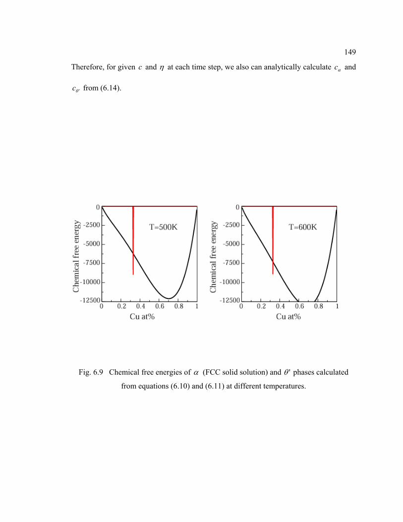
149

Therefore, for given c and η at each time step, we also can analytically calculate αc and

'θc from (6.14).

Fig. 6.9 Chemical free energies of α (FCC solid solution) and 'θ phases calculated

from equations (6.10) and (6.11) at different temperatures.

150


The third term in equation (6.7) represents the elastic energy associated with the

compositional and structural inhomogeneity. Since the mechanical equilibrium is often

established much faster than any other material processes, for any given microstructure,

the system is always at mechanical equilibrium

0=∂

∂

j

ij

rσ

(6.15)

)),,()(( 0 ηεελσ crr klklijklij −= (6.16)

where σij is the local elastic stress, rj is the jth component of the position vector, r, ijklλ is

the elastic stiffness tensor which may vary with space, εjk(r) is the total strain state at a

given position in a microstructure, and )(roklε is the local stress-free strain or

transformation strain or eigenstrain which is also a function of position through its

dependence on field variables. The method described in Chapter 3 will be used to obtain

the elastic solution of the mechanical equilibrium equation (6.15). Then, the elastic

energy density can be calculated

)(21),,( 0

ijijijelas crE εεση −= (6.17)

Since the stress-free strain )(roklε is a function of phase-field variables, the elastic energy

density depends on phase-field variables and thus the microstructure.

151

We employed two sets of phase-field variables, i.e., composition field c and order

parameter field η to describe the microstructure during the precipitation process in Al-Cu

alloys. For a given orientational 'θ variant, the stress-free strain )(roklε could be

described in three different ways

===

))(),(()())(()())(()(

00

00

00

rrcrrrrcr

ijij

ijij

ijij

ηεεηεε

εε (6.18)

Since the stress-free strains reflect the lattice mismatch, these different forms of stress-

free strains should be same in terms of the position vector, r, for a given microstructure.

However, we have notice that the driving force of microstructure evolutions is the

variation of total free energy with respect to the field variables, it is clear that the forms

of stress-free strains will affect the driving force, hence the microstructural evolution. For

simplicity, we assume the stress-free strains are a function of the order parameter field

variable η . It is written as

20

051.000000746.000000746.0

)( ηε

−=rij (6.19)

Therefore, the elastic energy density only depends on the order parameter field η .

152

6.2.3 Kinetic equations

In all phase-field models, the temporal and spatial evolution of the field variables

follows the same set of kinetic equations. A conserved field, composition field c ,

evolves with time according to the Cahn-Hilliard equation [31] (Cahn 1961), or simply

the diffusion equation in the case that no gradient energy is introduced for the conserved

variable, whereas the non-conserved fields, order parameter field η, are governed by the

Allen-Cahn equation [257] (Allen and Cahn 1977), i.e.

])2

)(([)()( 02

2

00 η

ηϕκηη

ϕδηδϕη

∂∂

Ω−∇∂∂

Ω−∂∂

−Ω

=−=∂∂ elaEGLFL

t (6.20)

))(),((cG

GTD

tc

cc ∂∂

∇⋅∇=∂∂ η

(6.21)

With the total free energy (6.6), they can be rewritten as

])(])(

)(

)()()[()2

)(([)(

0

22

00

ηη

ηηϕκη

ϕη

α

αα

θα

θθ

αα

∂∂

Ω−′−∂

∂−−

−′+∇∂∂

Ω−Ω

=∂∂

′

′′

elsEgwc

cfcc

cfcfhLt

(6.22)

)))(('),(()),((

))(),((

' ηηηη

ηη

θα

η

∇−⋅∇+∇⋅∇=

∇+∇⋅∇=∂∂

cchTDcTD

cGGG

TDtc

ccccc (6.23)

together with the constraint conditions,

θα ηη ′+−= chchc )())(1( , (6.24)

153

θ

θθ

α

αα

′

′′

∂∂

=∂

∂c

cfc

cf )()(, (6.25)

where ),( TD η is diffusion coefficient, and )(ϕL is interface mobility coefficient. In this

model there are two sets of variables ),( ηc and ),( 'θα cc . Their relationship is described

by equations (6.24 and 6.25).

6.3 Determination of model parameters

There are three unknown model parameters in the evolution equation (6.20 and

6.21), i.e., )(ϕL , )(ϕκ and w which relate to materials constants such as interface

mobility )(ϕM , interface thickness )(2 ϕλ and interface energy )(ϕσ . For a quantitative

simulation, we first need to establish the relationships between these model parameters

and material constants. To do so, we consider a system with a flat interface between two

coexisting isotropic phases 'θ and α . The system can be viewed as one-dimensional

problem. In the following sections, the relationships between model parameters and

materials constants will be derived by analyzing equilibrium and kinetic properties of

evolution equation (6.20 and 6.21) using 22 )1()( ηηη −=g and 32 23)( ηηη −=h .

6.3.1 Equilibrium solution

At equilibrium, both the order parameter field and composition field become

independent of time. Let )(0 xc and )(0 xη denote the equilibrium profiles of composition

and order parameter field in one dimension. If the effect of elastic energies on

154

equilibrium properties is ignored, and the gradient coefficient )(ϕκ is assumed to be

constant κ , from kinetic equations (6.20 and 6.21), we have

020

22

00

=Ω+∂∂

−xd

dG ηκ

η (6.26)

0))(),((0

0

00

=∂∂cG

dxd

GTD

dxd

cc

η (6.27)

At equilibrium the chemical potential should be constant throughout the system, hence,

equation (6.27) is equivalent to

ecG

cG

=∂∂

0

(6.28)

where ecG is constant.

From equations (6.6), (6.8) and (6.9), we have

θ

θθ

α

αα

′

′′

∂∂

=∂

∂=

∂∂

ccf

ccf

cG )()(

0

(6.29)

Therefore, )(xcα and )(' xcθ are constant, and equal to the equilibrium compositions,

ecxc αα =)( and

ecxc '' )( θθ = (6.30)

155

Substituting ecxc αα =)( and ecxc '' )( θθ = into equation (6.24), we have the equilibrium

composition

ee cxhcxhxc '000 ))(()))((1()( θα ηη +−= (6.31)

Now let us find the equilibrium solution )(0 xη of Equation (6.26). Substitute free energy

G (6.6) and solution (6.30) into equation (6.26), it becomes

0)('])(

)()()()[(' 0'''

020

22

0 =−∂

=∂−−−+Ω ηη

ηκ

α

ααα

θαθθ

αα wg

cccf

cccfcfhxd

d eeeee (6.32)

After multiplying dxd /0η on both sides of equation (6.32) and integrating it from

−∞=x to ∞=x , we get

0)(

)()()( ''' =

∂=∂

−−−α

ααα

θαθθ

αα

cccf

cccfcfe

eeee (6.33)

Equations (6.29) and (6.33) show the well-known equilibrium condition

ee

eee

ce

cc cccfcf

cfcfG'

''

'' )()(

)()('

θα

θθ

αα

θθ

αα

θα −−

=== (6.34)

156

Therefore, equation (6.33) can be rewritten

)( 020

22

0 ηη

κ gwdx

d ′=Ω (6.35)

Multiply dxd /0η on both sides of the equation above,

)()(21

0202

0 ηη

κ wgdxd

dxd

dxd

=Ω (6.36)

we have

)()(21

0202

0 ηη

κ wgdx

d=Ω (6.37)

Integrating equation (6.37) from −∞=x to ∞=x with 22 )1()( ηηη −=g and the

following boundary conditions,

0)1(,0)1(,1, =====−∞= ηηη hgx

0)0(,0)0(,0, =====∞= ηηη hgx (6.38)

0)(=

−∞=dx

xdη

0)(=

∞=dxxdη

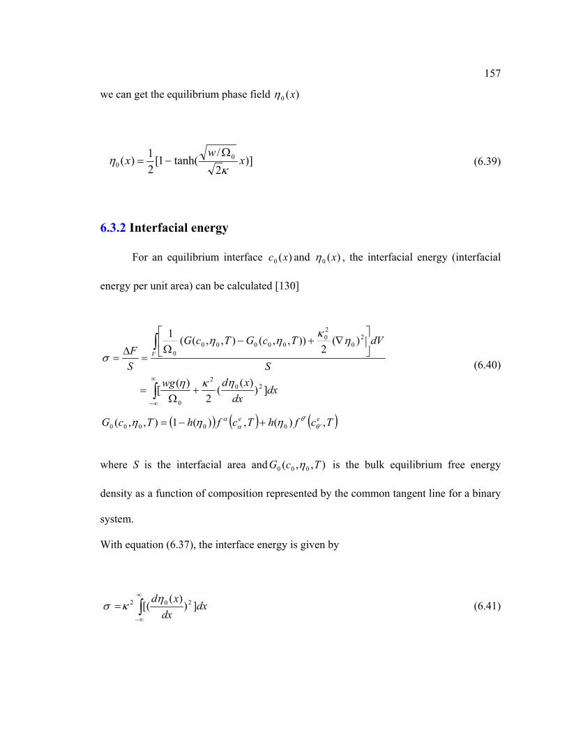
157

we can get the equilibrium phase field )(0 xη

)]2/

tanh(1[21)( 0

0 xw

xκ

ηΩ

−= (6.39)

6.3.2 Interfacial energy

For an equilibrium interface )(0 xc and )(0 xη , the interfacial energy (interfacial

energy per unit area) can be calculated [130]

dxdx

xdwgS

dVTcGTcG

SF V

]))(

(2

)([

)(2

)),,(),,((1

202

0

20

20

000000

ηκη

ηκ

ηησ

+Ω

=

∇+−

Ω=

∆=

∫

∫

∞

∞−

(6.40)

( ) ( ) ( )TcfhTcfhTcG ee ,)(,)(1),,( '00000 θθ

αα ηηη ′+−=

where S is the interfacial area and ),,( 000 TcG η is the bulk equilibrium free energy

density as a function of composition represented by the common tangent line for a binary

system.

With equation (6.37), the interface energy is given by

dxdx

xd])

)(([ 202 η

κσ ∫∞

∞−

= (6.41)

158

For an interface at equilibrium, the total gradient energy is half of the total interfacial

energy. Analytical expressions for the interfacial energy in terms of free energy

parameters and the gradient energy coefficients are only available for very simple cases

that an analytical solution for the equilibrium profile of field variable across the interface

can be derived. For example, in our case we have an analytical solution (6.39) with the

double well potential 22 )1()( ηηη −=g . Substitute the solution into equation (6.41), a

relationship between the interface energy and model parameters is obtained

23/ 0Ω

=wκ

σ (6.42)

From equation (6.39), we have

dxwgd 20

00

)(2κη

ηΩ

= (6.43)

If we define that ξηξ −≤≤ 10 is the interface, the interface thickness )2( λ can be

calculated by

00

01 2

0

/2

)(22

Ω=

Ω= ∫

−

wwgd κα

ηηκ

λξ

ξ

(6.44)

159

where α is a constant which depends on ξ (the definition of the interface). When

1.0=ξ , 2.2=α . When 05.0=ξ , 94.2=α . Equations (6.42) and (6.44) show the

relationship between model parameters (the height of double well potential w and

gradient coefficient κ ) and material constants (interface energyσ and interface

thickness λ2 ).

For the specific Al-Cu alloy system, 'θ precipitates have strong interface energy

anisotropy. A number of approaches have been proposed to describe the interfacial

energy anisotropy in phase-field models. One straightforward and most often employed

approach is to make the square root of the gradient coefficient have the same directional

dependence as the interfacial energy (according to relation (13)). Another approach is to

add higher order gradient energy terms [258-261]. In the present work, the interfacial

energy anisotropy is described in terms of the normal of the interface as

≤≤−−+−≤≤+−++−≤≤−++

+=

2/2/),sin(12/2/),cos(1

2/2/),sin(1

1)(

021

00

0210

πϕϕπϕγγϕπϕϕπϕγϕπϕπϕγγ

γσ

ϕσ (6.45)

where 0σ is the interfacial energy at 0=ϕ , )sin(/)cos( 001 ϕϕγγ = , )sin(/ 02 ϕγγ = , γ

is determined by the interfacial anisotropy, and 200/0 πϕ = is chosen as a very small

angle to describe the cusps [262]. Equation (6.45) reflects a cylindrical symmetry of the

interfacial energy for plate-like 'θ precipitates. The gama plot of the interface energy has

160

two cusps at 2/πϕ ±= for describing the flat interface of 'θ precipitates. As a result,

the interfacial energy along the edge is assuming isotropic.

6.3.3 Thin-interface limit

In this section we focus on deriving the relationship between the phase field

mobility coefficient and the interface kinetics coefficient, which is a proportionality

constant between the driving force for an interface motion and the interface moving

velocity. Let us consider a system with a flat interface which moves with a constant

velocity V. In a moving coordinate system with the same velocity V, we can rewrite

kinetic equations (6.20) and (6.21) by using the following transformations

tVxx −=' , tt ='

)(),( 'xctxc = , )(),( 'xtx ηη = (6.46)

'

'

'

' )(),(x

Vtx

xtx

ttx

∂∂

−=∂∂

∂∂

=∂

∂=

∂∂ ηηηη

'''

' )(),(xx

xxx

xx

tx∂∂

=∂∂

∂∂

=∂

∂=

∂∂ ηηηη

where 'x is the coordination in the moving coordinate system. In the new coordinate

system, the equations (6.20) and (6.21) are rewritten as

161

)](])(

)()()()[('

[' 2

22

00

ηηηκη

α

αα

θαθθ

αα gw

ccf

cccfcfhdxdL

xV ′−

∂∂

−−−′+ΩΩ

=∂∂

− ′′′

(6.47)

))('

),(('' α

αα

η cfdxd

GTD

dxd

xcV c

cc

=∂∂

− (6.48)

Integrating equation (6.48) from λ−='x to 'x

λα

α

λα

αα

αθ

ηη

ηη

α

αα

−=

−=

−=

−=−−

'

'

int'

')'()()(

')(

)('

)()('

)(])'([

xcc

ccc

cc

xc

ccc

cc

dxxdcG

GDcf

dxd

GD

cfdxd

GDcf

dxd

GDcxcV

(6.49)

where int'θc is the composition of 'θ phase at the interface λ−='x . Assume

0.0)('

=−= λ

ηx

D or 0.0')'(

'

=−= λxdx

xdc , then

])'([)(

)('

int'θα

α

ηαcxcV

DGcf

dxd cc

c −−= (6.50)

Since )()( ''' θ

θα

αθα

cfcf cc = , we have

])'([)(

)('

int''

'' θθ

θ

ηθcxcV

DGcf

dxd cc

c −−= (6.51)

162

Integrating equation (6.50) and (6.51) from λ−='x to 'x ,

dxcxcVDG

cfcfx

cccc ∫

−

−−=λ

θαα

αα

ηαα])([

)()()( int

'int (6.52)

dxcxcVDG

cfcfx

cccc ∫

−

−−=λ

θθθ

αα

ηθα])([

)()()( int

'int

'''

(6.53)

Assume there is a very small fluctuation in composition profile of traveling wave, to first

order,

ααα δccc e +=

''' θθθ δccc e +=

ααα

αα

αα δ

αccfcfcf e

ce )()()( += (6.54)

''''

'' )()()(

' θθθ

θθ

θθ δ

θccfcfcf e

ce +=

ααα

αα

αα δ

ααααccfcfcf e

cce

cc )()()( +=

we have

)()()()(

)()()(()()()()(

'''

''''

αα

θαθθ

αα

αα

αα

θααα

θαθθ

αα

α

ααα

cfcccfcf

cfcfcccfcccfcf

ceeee

ecc

eec

−−−=

−−−=−−− (6.55)

163

Multiply eq.(6.47) with 'dx

dη , and integrate from [-λ, λ],

ηηη

α

αα

θαθθ

αα

λ

λ

dhc

cfcccfcfdxdxd

LV )(])()()()([')

'(

0

1

20 ′

∂∂

−−−=Ω

− ∫∫ ′′′

−

(6.56)

Using equation (6.51), (6.55) and )()()()( ''' e

ceeee cfcccfcf α

αθαθ

θα

αα

−=− ,

ηηη

η

λθθα

λ

λ

θθ

αα

θα θα

dhdxcxcDGccdx

dxd

L

cfcfccV

xccee

ce

cee

)()'])'([)(

()(')'

(

))()()((0

1

int''

20

int'

'' '

′−−+Ω

−−=

∫ ∫∫−−

(6.57)

To the first order in the Peclet number, DVp ~/2λ= ( D~ is average interface diffusivity),

and assume )'()'( 0 xx ηη = and )'()'( 0 xcxc = , we can calculate interface velocity V for

given interfacial mobility coefficient L by

−−Ω

= )]()[(1 int'

''

0' θ

θθα θ

cfGccMV cec

ee (6.58)

Where M is the interface kinetic coefficient,

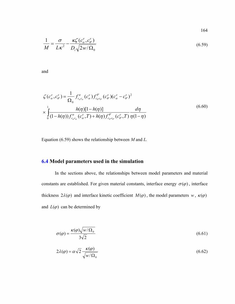
164

0

'2 /2

),(1Ω

−=wD

ccLM i

eeθακζ

κσ

(6.59)

and

)1(),()(),())(1()](1)[(

))(()(1),(

1

0 ''

2''

'

0'

''

''

ηηη

ηηηη

ζ

θθ

αα

θαθθ

αα

θα

θθαα

θθαα

−+−−

×

−Ω

=

∫d

TcfhTcfhhh

cccfcfcc

ecc

ecc

eeecc

ecc

ee

(6.60)

Equation (6.59) shows the relationship between M and L.

6.4 Model parameters used in the simulation

In the sections above, the relationships between model parameters and material

constants are established. For given material constants, interface energy )(ϕσ , interface

thickness )(2 ϕλ and interface kinetic coefficient )(ϕM , the model parameters w , )(ϕκ

and )(ϕL can be determined by

23/)(

)( 0Ω=

wϕκϕσ (6.61)

0/)(2)(2Ω

=wϕκαϕλ (6.62)

165

0

'2

/2),()(

)(1

1)()()(

Ω+

=

wDcc

M

L

i

eeθαζϕκ

ϕϕκϕσϕ (6.63)

Input parameters in simulations include the grid spacing x∆ , the interface thickness 12λ ,

the constant α in equation (6.62), the interfacial energies of semi-coherent interface,

mole volume 0Ω , and 0ϕ in equation (6.45). With these parameters, the model

parameters w , )(ϕκ can be determined. For example, consider the 'θ precipitate shown in

Fig. 6.8, with nmx 1=∆ , the semi-coherent interface thickness of 'θ precipitates

x∆= 62λ at 0=ϕ , the interfacial energy 21 /600 mmJ=σ , mole volume

molm /10 350

−=Ω , and 2.2=α , the height of the double potential can be calculated

from equation (6.61) and (6.62).

λασ

26 1=w (6.64)

The coherent interface energy at 2/πϕ = is taken to be 22 /200 mmJ=σ . From

equation (6.61) and (6.45) with the values of 1σ , 2σ and 200/0 πϕ = , )(ϕκ can be

fitted. Since there is no available experimental data of interface kinetic coefficient )(ϕM ,

the interface mobility coefficient )(ϕL are artificially defined as

166

≤≤−−+−−≤≤+−++−≤≤−++

+=

2/2/),sin(12/2/),cos(12/2/),sin(1

1)(

012

00

0120

πϕϕπϕββϕπϕϕπϕβϕπϕπϕββ

βϕ

LL (6.65)

where 0L is the interface mobility coefficient at 0=ϕ , )sin(/)cos( 001 ϕϕββ = ,

)sin(/ 02 ϕββ = , and β is determined by the interface mobility anisotropy.

200/0 πϕ = is chosen as a very small angle, which implies that only the broad interface

has a very small mobility. In simulations, the system is assumed to be elastically

homogeneous. The elastic constants of Al-Cu alloys [243] are

GPaCGPaCGPaC 29;61;108 441211 ===

For simplicity, assume that the diffusion coefficient ),( TD η only depends on

temperature T [180],

−=

RTQDTD exp)( 0 6.66)

where scmD /45.0 20 = , molkcalQ /8.31= , and R is the universal gas constant. The

precipitate temperature KT 500= is used in simulations.

167

Using dimensionless variables 20

* / ltDt = and lxx /* = where l represents the

grid spacing ( x∆ ) or the characteristic length, the kinetic equations (6.22) and (6.23) are

simplified to

])(])()(

)()()[()()[(

**

*

***2****

ηη

ηηϕκϕη

α

αα

θα

θθ

αα

∂∂

−′−∂

∂−−

−′+∇⋅∇=∂∂

′

′′

elsEgwc

cfcc

cfcfhLt

(6.67)

)))((')(())(( *'

****** ηη θα ∇−⋅∇+∇⋅∇=

∂∂ cchTDcTDtc

(6.68)

where

0

*

44

*

044

*

044

''

''*

044

*2

44

2*

0

244*

)()(;;

;)(

)(,)(

)(;)()(;)()(

DTDTD

CEE

Cww

Ccf

cfC

cfcf

lCDlCLL

elsels ==

Ω=

Ω=

Ω=== θ

θ

θθα

α

ααϕκϕκ

ϕϕ

In simulations, periodic boundary conditions in x-, y- and z-directions are employed. The

kinetic equations are solved numerically using Fourier-Spectral method [159].

6.5 Results and discussions

Extensive testing on the dimensionless time *t and the grid spacing or the

characteristic length xl ∆= were first conducted to ensure the stability of numerical

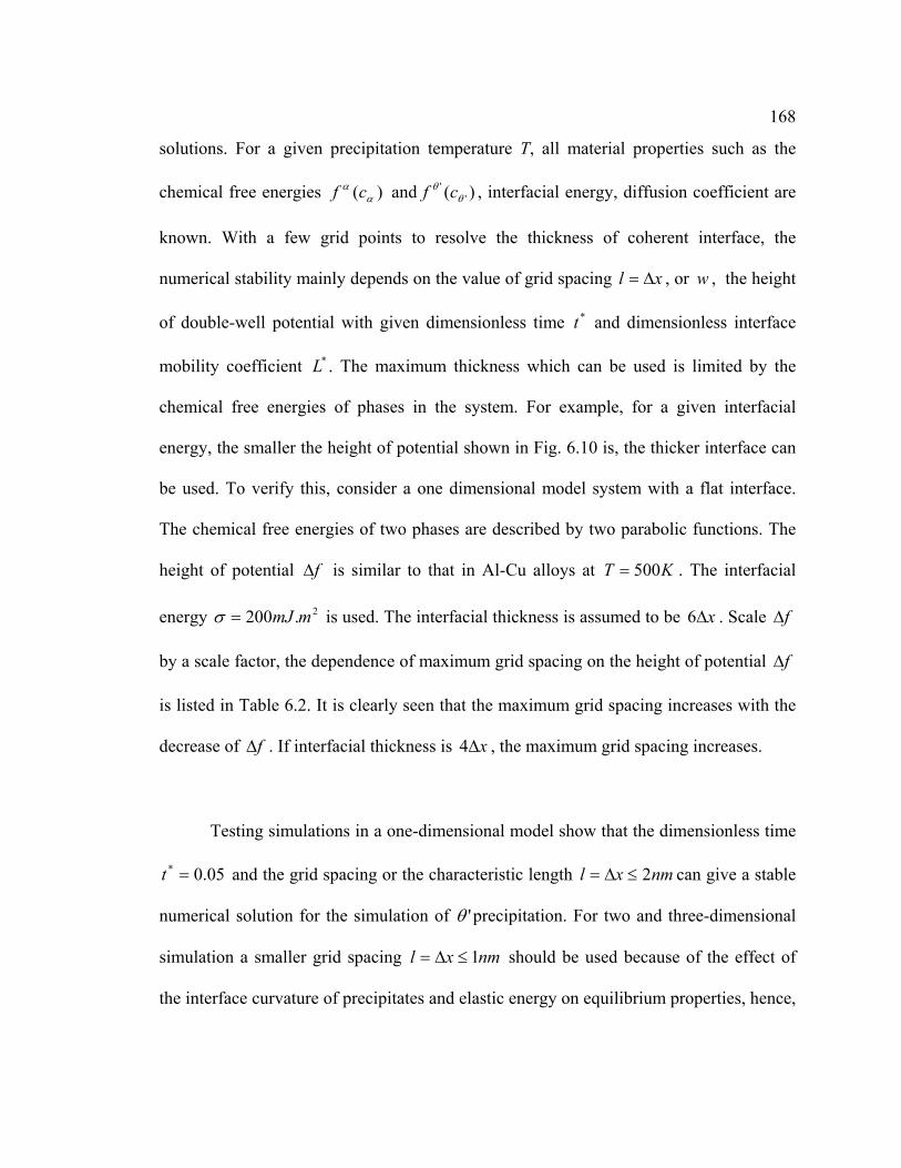
168

solutions. For a given precipitation temperature T, all material properties such as the

chemical free energies )( αα cf and )( '

'θ

θ cf , interfacial energy, diffusion coefficient are

known. With a few grid points to resolve the thickness of coherent interface, the

numerical stability mainly depends on the value of grid spacing xl ∆= , or w , the height

of double-well potential with given dimensionless time *t and dimensionless interface

mobility coefficient *L . The maximum thickness which can be used is limited by the

chemical free energies of phases in the system. For example, for a given interfacial

energy, the smaller the height of potential shown in Fig. 6.10 is, the thicker interface can

be used. To verify this, consider a one dimensional model system with a flat interface.

The chemical free energies of two phases are described by two parabolic functions. The

height of potential f∆ is similar to that in Al-Cu alloys at KT 500= . The interfacial

energy 2.200 mmJ=σ is used. The interfacial thickness is assumed to be x∆6 . Scale f∆

by a scale factor, the dependence of maximum grid spacing on the height of potential f∆

is listed in Table 6.2. It is clearly seen that the maximum grid spacing increases with the

decrease of f∆ . If interfacial thickness is x∆4 , the maximum grid spacing increases.

Testing simulations in a one-dimensional model show that the dimensionless time

05.0* =t and the grid spacing or the characteristic length nmxl 2≤∆= can give a stable

numerical solution for the simulation of 'θ precipitation. For two and three-dimensional

simulation a smaller grid spacing nmxl 1≤∆= should be used because of the effect of

the interface curvature of precipitates and elastic energy on equilibrium properties, hence,

169

numerical stability. Therefore, the grid spacing nmxl 1=∆= and 05.0* =t are used in all

simulations except for very special cases.

Table 6.2 The dependence of maximum grid spacing on the height of potential f∆

Scale factor x∆ (10-9m) w (J/mol) ∆f (J/mol)

1 0.4 22000 7500

0.2 1.8 3666 1500

0.1 3.5 1650 750

0.02 18 366 150

0.002 200 26 15

170

Fig. 6.10 The height of chemical potentials in two phase equilibrium system.

171

6.5.1 Velocity of a flat interface

Based on the discussions presented in the last several sections, the interface

mobility coefficient *L is the only remaining parameter to be determined. To evaluate the

role of this parameter, a one-dimensional model of 'θ precipitate growth is considered.

The velocity of a flat interface and composition evolutions are simulated for different

values of *L . Fig. 6.11 shows a 'θ precipitate placed in the center of a simulation cell.

The size of the precipitate and the simulation cell are x∆40 and x∆2048 , respectively.

x∆ is 0.5nm. The initial composition is set to be the equilibrium composition c=0.33 in

the precipitate and c=0.08 in the α phase (the solid solution). The moving distance of the

interface as a function of time and square root of time is presented in Fig. 6.12a and Fig.

6.12b, respectively. It can be clearly seen that the relationship between the moving

distance and time becomes increasingly linear as *L decreases, and more parabolic

as *L increases. These reveal a fact that the model parameter *L can be used to describe

the growth of 'θ precipitates either interface-controlled or diffusion-controlled. For the

set of model parameters of Al-Cu alloys at KT 500= , the simulation results illustrate

that when 05.0* <L , the growth is interface-controlled, and diffusion-controlled when

50* >L .

In one dimension, the growth of a 'θ precipitate can also be modeled using the

commercial program (DICTRA) [263] assuming a sharp interface and purely diffusion-

controlled growth. In the case of constant diffusion coefficient, one can easily find an

analytic solution for the growth kinetics. Fig. 6.13 presents a comparison of the evolved

172

composition profiles obtained by the phase-field simulation and calculated with an

analytical solution. Dashed lines and solid lines represent the analytical solution and the

numerical solution, respectively. It can be seen that the evolved composition profiles

obtained by two methods are in good agreement except at the interface region where the

analytical solution has a sharp interface while the phase-field solution has a diffusion

interface.

Fig. 6.11 One-dimensional model of a 'θ precipitate growth.

173

(a)

(b)

Fig. 6.12 Moving distance of the interface as a function of time, (a) vs t (b) vs t

174

Fig. 6.13 Comparison of composition profiles obtained by the phase-field simulations and

analytical solutions at different times.

175

6.5.2 Equilibrium shape of an isolated 'θ precipitate

In this section, the equilibrium shape of an isolated 'θ precipitate in two

dimensions is simulated. The equilibrium shape is determined by the minimization of the

total free energy of the system which includes interface energy and elastic energy. The

kinetic process, i.e., how the precipitate reaches its equilibrium shape, should not affect

the equilibrium shape. Therefore, the simulations take the interface energy anisotropy and

elastic energy into account while the interface mobility anisotropy is ignored. In the

simulations, an elliptic 'θ precipitate with a long axis xa ∆= 45 and a short axis

zb ∆= 20 is initially placed in the center of the simulation cell zx ∆×∆ 128256 . The

precipitate and the matrix are assigned their equilibrium compositions, 33.0=c and

0072.0=c , respectively. The thickness of the coherent interface is assumed to be x∆6 .

In order to eliminate the effect of grid numerical pinning, a smaller grid size

nmxz 333.0333.0 =∆=∆ in z-direction is used. As a result, the dimensionless time

*t should be reduced. Fig. 6.14 shows the evolution of an initially non-equilibrium

precipitate without the contribution of elastic energy. The blue region denotes the matrix

and the red for the precipitate. The transition region of the color implies the interfacial

region. Since the interfacial energy of the coherent interface ( 21 /200 mmJ=σ ) is lower

than that of the semi-coherent interface ( 21 /600 mmJ=σ ), it can be seen that the

thickness of the coherent interface is smaller than that of the semi-coherent interface. The

composition evolution along the long and short axes of the elliptic precipitate is showed

176

Fig. 6.14 Morphological evolution of a precipitate from an initially non-equilibrium shape to equilibrium in the absence of elastic energy.

177

(a)

(b)

Fig. 6.15 Composition evolution, (a) along the long axis, and (b) along the short axis of the elliptic precipitate in the absence of elastic energy.

178

in Fig. 6.15a-b, respectively. It is found that the initially elliptic precipitate becomes a

plate-like precipitate at equilibrium. The aspect ratio of the equilibrium precipitate is

close to 3 as it can be expected from the Wulff construction. A closer observation shows

that the equilibrium compositions in both precipitate and matrix are slightly higher than

that calculated from the chemical free energies. It can be explained with the Gibbs

Thomson effect that the solubility increases with the decrease of precipitate size or the

curvature increase of precipitate interfaces.

Fig. 6.16 shows the morphological evolution of the precipitate with the

contribution of elastic energy. It can be seen that the effect of stresses around the 'θ

precipitate on the equilibrium shape is obvious. From the stress-free strain tensor (6.19)

associated with the 'θ precipitate, it is found that the maximum component of the stress-

free strain is 051.0*33 −=ε , which generates a large tensile stress 33σ in both precipitate

and matrix. A thinner precipitate results in a lower elastic energy. Unlike the case without

elastic energy, the thickness of the precipitate is smaller in the presence of the elastic

energy, i.e., the elastic energy increases the aspect ratio of the precipitate. In this case the

aspect ratio is about 8.5. The composition evolution along the long and short axes of the

elliptic precipitate is showed in Fig. 6.17a-b. It can be seen that the presence of elastic

energy shifts the equilibrium composition in both the precipitate and the matrix.

179


shape to equilibrium in the presence of elastic energy.

180

(a)

(b)


the elliptic precipitate in the presence of elastic energy.

181

6.5.3 Growth of an isolated 'θ precipitate

In this section, the phase-field model is employed to study the growth behavior of

a single 'θ precipitate. In the simulations, the interfacial energy and mobility are

described by functions (6.45) and (6.65), respectively. The model parameters are

20 /600 mmJ=σ , 2=γ , 1000=β and 100*

0 =L . The nucleation process of the

precipitate is ignored, so an elliptic 'θ precipitate with a long axis xa ∆= 40 and a short

axis zb ∆= 20 is initially placed in the center of the simulation cell zx ∆×∆ 512256 . The

initial composition in the precipitate and the matrix are 33.0=c and 05.0=c ,

respectively. The thickness of the coherent interface is assumed to be x∆6 . In order to

eliminate the effect of grid numerical pinning, a smaller grid size

nmxz 333.0333.0 =∆=∆ in z-direction is used. Fig. 6.18 and Fig. 6.19 show the

morphological evolution of the single precipitate without and with the elastic energy,

respectively. The figures are contours of composition field. The white lines in the figure

show the contour lines with 03.0=c . From Figs. 6.18 and 6.19, it is found that the

stresses associated the lattice mismatch between the precipitate and the matrix speed up

lengthening and slow down thickening. The composition evolution along the length and

thickness directions is plotted in Fig. 6.20 and Fig. 6.21. It can be clearly seen that the

velocity of the interface decreases as time increases. Fig. 6.22 plots the moving distance

of the interface as a function of time. These curves are fitted with non-linear functions.

For example, the thickness is described by ntHHH 10 += . For comparison, the fitted

curves are also plotted in the Fig. 6.22 with solid or dashed lines. A large fitting error

demonstrates that one function cannot completely describe the whole growth process.

182

The precipitate growth might be separated into three stages, i.e., at initial stage, growth

stage and later growth stage. At the initial stage, because a small precipitate with a sharp

interface is put into the simulation cell, such an initial condition might be different from

that in a real situation. The precipitate undergoes an initial relaxation in both composition

and shape. At the latter growth stage, the interaction among precipitates due to periodic

boundary conditions becomes strong. Therefore, for the growth behavior of an isolated

precipitate, the data at initial and later growth stage should be removed. The fitted curves

and functions are redrawn in Fig. 6.23. These results show that the thickening follows

3/2t law. Elastic energy affects the lengthening law, which leads to a faster lengthening

and a slower thickening compared with the case without elastic energies. The growth

behavior of an isolated precipitate is also simulated for an extreme case, i.e., the coherent

interface is almost immobile. In this case, a smaller interface mobility coefficient

2000=β in the coherent interface, and a larger grid spacing nmxz 1=∆=∆ in z-

direction are used. The other model parameters are the same as that in the previous case.

Fig. 6.24 shows lengthening and thickening without elastic energies for different initial

thickness nmandH 3630,24( 0 = ). It is evident that the length increases linearly while

the thickness remains the same for different initial thickness. The thinner the precipitate

is, the faster it grows. In the presence of elastic energy, the lengthening and thickening

kinetics are plotted in the Fig. 6.25. One can reach the same conclusion, i.e., elastic

energy speeds up the lengthening of the precipitates.

183


field in the absence of elastic energy. The white line is a contour of composition

03.0=c .

184


field in the presence of elastic energy. The white line is a contour of composition

03.0=c .

185


thickness direction in the absence of elastic energy.

186


thickness direction in the presence of elastic energy.

187

Fig. 6.22 Lengthening and thickening of an isolated precipitate.

188

Fig. 6.23 Lengthening and thickening of an isolated precipitate at the growth stage.

189

Fig. 6.24 Lengthening and thickening of a precipitate without elastic energy and the

coherent interface is immobile.

190

Fig. 6.25 Lengthening and thickening of a precipitate with elastic energy and the coherent

interface is immobile.

191

6.5.4 Coarsening of two precipitates in two dimensions

Coarsening is driven by the reduction in the interface energy. During coarsening,

the oversize size of precipitates increases. As a result, elastic energy increases. If the

change in the elastic energy during coarsening is comparable to the change in the

interface energy, the coarsening process depends on the competition between the

interface energy decrease and elastic energy increase. In the simulations, two precipitates,

a small one and a large one, are placed in the simulation cell. It is checked that the size of

the small one is larger than the critical size. The simulation cell and model parameters are

the same as that used in section 6.5.3, but the precipitate and the matrix have their own

equilibrium compositions 33.0=c and 0072.0=c , respectively. Fig. 6.26 and 6.27 show

the morphological evolution for the cases without and with elastic energies, respectively.

It can be found that the small precipitate gradually disappears in both cases. After that,

the single precipitate will reach its equilibrium shape as presented in section 6.5.2.

Notice the time shown in the figure, it can be seen that the elastic energy slows down the

coarsening process. These results demonstrate that the developed phase-field model can

properly describe the coarsening process.

192

Fig. 6.26 Coarsening of two precipitates in the absence of elastic energy.

193

Fig. 6.27 Coarsening of two precipitates in the presence of elastic energy.

194

6.5.5 Growth of multi-precipitates in two and three dimensions

All derivations in section 6.2 are carried out for one 'θ orientational variant 3η

which has a coherent interface with a normal direction 001 . In three dimensions, there

are three orientational variants. The function )(ηh and )(ηg are replaced by

)(2)(3),,( 33

32

31

23

22

21321 ηηηηηηηηη ++−++=h

23

22

21

41

42

23

43

41

22

43

42

21

23

22

21

23

22

21

43

42

41

33

32

31

23

22

21321

)()()(

)(

)()(2)()),,((

ηηηηηηηηηηηη

ηηηηηη

ηηηηηηηηηηηη

+++++++

+++

+++++−++=g

(6.69)

The stress-free strain tensor is defined as

23

22

21

0

051.000000746.000000746.0

00746.0000051.000000746.0

00746.000000746.0000051.0

)(

η

η

ηε

−+

−+

−=rij

(6.70)

The chemical free energy and total free energy of the system are given by

( ) ( )( ) ),,(,),(

,),,(1),,,,(

321'3,21

321321

ηηηηηη

ηηηηηη

θθ

αα

wgTcfh

TcfhTcG

++

−=′

, (6.71)

195

xdEk

TcGTcFV

elast

ii

i 323

1

2

3210

321 ]2

)(),,,,(1[),,,,( ∫ ∑ +∇+

Ω=

=

ηϕ

ηηηηηη (6.72)

where iϕ is the angle between two normal directions of interface at x and broad

interface of the ith 'θ precipitate variant.

Kinetic equations of the order parameter fields and concentration field can be

described as,

])2

)(([)()( 02

2

00 i

ela

ii

ii

i

ii

i EGLFLt η

ηϕκ

ηηϕ

δηδϕ

η∂∂

Ω−∇∂∂

Ω−∂∂

−Ω

=−=∂∂

(6.73)

))(),,(

( 3,21

cG

GTD

tc

cc ∂∂

∇⋅∇=∂∂ ηηη

(6.74)

with the constraint conditions

( )[ ] ( ) '321321 ,,,,1 θα ηηηηηη chchc +−=

( ) ( )'

''

θ

θθ

α

αα

ccf

ccf

∂∂

=∂

∂ (6.75)

It is clear that three variables ,, 21 ηη and 3η are equivalent in the phase-field model

described above. If any two of the three variables are equal to zero, the kinetic equations

are degenerated to equations (6.20) and (6.21). Therefore, all results deduced in section

(6.2) are applicable to any one of ,, 21 ηη and 3η .

196

In the simulations of the growth of multi-precipitates in two and three dimensions,

an uniform grid spacing ( nmzyx 1=∆=∆=∆ ) are employed to enlarge the simulation

cell and time step *t . The same expressions (6.45) and (6.65) and parameters:

20 /600 mmJ=σ , 2=γ , 1000=β and 100*

0 =L are used just by replacing ϕ with iϕ .

Simulation results show that the coherent interfaces are mobile with such an uniform grid

and interface mobility anisotropy. Some extent of numerical grid pinning is observed at

the coherent interface because the grid spacing is a little large for coherent interfaces, to

completely eliminate the grid pinning the grid spacing should be nmzyx 33.0=∆=∆=∆ .

6.5.5.1 Growth of multi-precipitates in two dimensions

60 small precipitates with different sizes are randomly placed into a 2D

simulation cell xx ∆×∆ 10241024 . In the precipitates, the composition is 33.0=c , and the

order parameter fields 1η or 3η are assigned to be 1 which depends on the orientation of

the precipitates. In the matrix, the composition is 05.0=c , and the order parameter fields

1η and 3η are assigned to be 0. The morphological evolutions of the precipitates are

shown in Fig. 6.28. It can be clearly seen that the lengthening of precipitates is much

faster than thickening, which consists with experimental observations. Some typical

configurations of precipitates are the same as that observed in the experiments shown in

Fig. 6.29. For example, when one precipitate hits another precipitate which has a

different orientation, it stops growing. As a result, a “T” like precipitate configuration is

formed as marked by “ T ” in the Fig. 6.28 and 6.29. When two precipitates with same

orientations grow in opposite directions and hit each other, they connect or coarsen only

197

if the spacing between the precipitates is very small as marked by “ C ” in the Figures.

The simulation results reveal that the coarsening behavior of plat-like precipitate should

be totally different from that of spherical precipitates, which could be explained by the

difference in composition fields and precipitate shapes. For plate-like precipitates the

composition field with large gradient is localized around the ram of the precipitate, which

is a very small fraction of the interface area while localized around the whole interface

for a spherical precipitate. Two particles connect or coarsen depends on the overlap of

their composition and/or parameter fields. As a result, the connection and coarsening of

plate-like precipitates are mostly controlled by the interaction among the fields around

the rams of precipitates. Therefore, the probability of connection or coarsening of two

plate-like precipitates is small compared to spherical precipitates. More simulations are

needed to reveal the coarsening behavior of 'θ precipitates. This will be left for future

work.

198

Fig. 6.28 Growth of multi-precipitates in two dimensions.

199

Fig. 6.29 SEM graph of 'θ precipitates from Weiland [180].

200

6.5.5.2 Growth of multi-precipitates in three dimensions

Because of the limitation of computer resources, it is hard to perform a large-scale

3D simulation even with a parallel code. However, to demonstrate the performance of the

developed phase-field model in 3D, the growth of two precipitates is simulated in a small

simulation cell xxx ∆×∆×∆ 12864128 . The simulation includes interface energy

anisotropy, interface mobility anisotropy and elastic energy. In the precipitates, the initial

composition is 33.0=c , and the order parameter fields 2η or 3η are assigned to be 1

which depends on the orientation of the precipitates. The composition is 05.0=c , and

the order parameter fields 1η and 3η are assigned to be 0 in the matrix. Fig. 6.30 shows

the morphological evolution of the precipitates. Comparing Fig. 6.2 and Fig. 6.30, it can

be found that the simulation reproduces a similar precipitate morphology observed in the

experiments [180]. Although the model can be used to study and reveal the fundamental

features and mechanisms about plate-like precipitate growth in 1D, 2D and 3D,

challenges remain. These include increasing the length and time scales, and extending the

model to multi-component systems.

201

Fig. 6.30 Growth of two precipitates in three dimensions.

202

6.6 Conclusion

A phase-field model which can automatically incorporate the thermodynamic and

kinetic information from databases is developed for studying the precipitation of 'θ phase

in Al-Cu alloys. In addition, the relationships between model parameters and material

thermodynamic and kinetic properties are established, which enable people to

quantitatively simulate the microstructure evolution in material processes. Systematical

test in 1D, 2D and 3D has been carried out. The growth of a single 'θ precipitate in 1D

exactly reproduces the results from analytical solutions. The equilibrium shape simulated

in two dimensions is in good agreement with that predicted by the Wulff construction

based on the interface energy anisotropy. 2D and 3D simulations produce typical

precipitate morphologies and precipitate configurations which are observed in the

experiments. The simulation results show that the lengthening and thickening laws of an

isolated precipitate in 2D depends on the mobility of coherent interface and the elastic

energy. If the coherent interface is immobile, the lengthening follows t law while the

thickness remains no change during growth. The elastic energy associated with the

lattice mismatch between the precipitate and the matrix speeds up the lengthening, but

slows down the thickening and coarsening process. All simulation results demonstrate

that the developed phase-field model is able to simulate the precipitation of 'θ in Al-Cu

alloys, which involves plate-like precipitates, strong interface energy anisotropy,

interface mobility anisotropy and elastic energy.

203

Chapter 7

Conclusions and Future Directions

7.1 Conclusions

In this thesis, the phase-field approach is applied to a number of microstructure

problems involving elastic inhomogeneity, structural defects such as dislocations, and

precipitates with strong interfacial energy and mobility anisotropy. The main

contributions to the phase-field theory includes:

(1) An efficient iteration method is proposed to solve the mechanical equilibrium

equations in a solid with elastic inhomogeneity, even with voids or a vapor phase

where the elastic constants are zero. Therefore, the phase-field model can be

extended to study the effect of strongly elastic inhomogeneity on microstructure

evolutions, and simulate microstructure evolutions in films with curved surface

and subject to substrate constraint.

(2) The structural defects such as dislocations are introduced into the phase-field

model with the concept “eigenstrain” in mesomechanics. Two unique features are

realized. The first one is that the lattice distortion due to structural defects and

compositional and/or structural inhomogeneity is expressed with one eigenstrain

tensor. The calculation of elastic energy is computationally efficient, particularly

for three-dimensional cases. The second is that it becomes particularly convenient

204

to simulate defect dynamics. As a matter of fact, phase-field models of

dislocation dynamics [87,88] is based on the same idea proposed in this thesis.

(3) A general phase-field model of dislocation dynamics in an alloy with mobile

dislocations, diffusive solutes and immobile defects such as inclusions is

developed. A new eigenstrain function of a dislocation loop is constructed, which

eliminate the dependence of dislocation Burgers vector on applied stresses in the

original phase-field model of dislocation dynamics. As a result, it provides a

correct dislocation stress field for both static and moving dislocations. This model

can be applied to study the strengthening of alloys.

(4) A phase-field model is extended to simulate the precipitation of 'θ phase in Al-Cu

alloys. The effect of elastic energy associated with the lattice mismatch between

'θ precipitates and matrix, the interface energy anisotropy and the interface

mobility anisotropy on the growth of 'θ precipitates are taken into account. The

relationships between phase-field model parameters and thermodynamic and

kinetic data of alloys are established, which is the basis for quantitative

simulations. A systematic testing of the growth of 'θ precipitates is performed in

1D, 2D and 3D with the developed model. The results demonstrate the potential

applications to simulating the growth of precipitates with abnormal shape such as

plate-like and needle-like precipitates.

205

7.2 Future directions

The phase-field models developed in this thesis could further be improved or

applied to other interesting microstructure problems. For example:

(1) The formation of three-dimensional islands or self- assembly microstructure patterns

on a substrate is of both scientific interest and technological importance. The

developed phase-field model in a solid with elastic inhomogeneity is applicable to

studying such a material process.

(2) The phase-field model of dislocation dynamics is able to correctly describe the

elastic interaction among coherency microstructures, dislocations and other

defects, the dislocation multiplication by Frank-Read mechanism, and dislocation

annihilation. However, it cannot take the crystal friction resistance, dislocation

climb and dislocation reactions such as dissociation into account. To incorporate

these features into the model will broaden its practical applications.

(3) For the phase-field model of the precipitation of 'θ precipitates in Al-Cu alloys, it is

desired to increase the simulation time step and simulation cell size for a practical

application. To do so, the following three aspects could be explored: the efficient

numerical method for solving the kinetic equations, a similar adaptive or multi-

scale treatment in coherent interfaces and multi-time scale methods. A practical

alloy is usually a multi-component system. Therefore, it will be important to

extend the model to a multi-component system. In addition, experimental

206

observation shows that defects such as dislocations are preferential nucleation

locations for 'θ . Therefore, it will be interesting to study the nucleation near

dislocations.

207

References

[1] A.G. Khachaturyan. Theory of Structural Transformations in Solids. Wiley, New

York, 1983.

[2] T. Mura. Micromechanics in Solids. Kluwer Academic, Dordrecht, 1982.

[3] M. Doi. Prog. Mater. Sci., 40, 79(1996).

[4] P. Fratzl and O. Penrose, et al. J. Stat. Phys., 95, 1429(1996).

[5] P.W. Voorhees and G. B. McFadden, et al. Acta Metall. Mater., 40, 2979(1992).

[6] L.Q. Chen and Y.Z. Wang. J. Miner. Met. Mater. Soc., 48, 13(1996).

[7] W. Baravosa-Carter and M.J. Aziz. Phys. Rev. Lett., 81, 1445(1998).

[8] M.J. Aziz, P.C. Sabin and G.Q. Lu. Phys. Rev., B44, 9812(1991).

[9] P.W. Voorhees and M.J. Aziz. In Interfaces for the Twenty-First Century: New

Research Directions in Fluid Mechanics and Materials Science, eds. M.K. Smith,

M.J. Miksis, G.B. McFadden, G.P. Neitzel and D.R. Canright, Imperial College

Press, London, 167(2002).

[10] The mechanism of phase transformations in metals, A Symposium organized by the

Institute of Metals and held at the Royal Institution, London, Richard Clay and

Company, 1956.

[11] A.P. Levanyuk and A.S. Sigov. Defects and structural phase transitions, Vol.6,

Gordon and Breach Science Publishers, New York, 1988.

[12] J.A. Krumhansl. Phase Transitions, B65, 109(1998).

[13] M.I. Katsnetson and A.V. Trefilov. Phys. Metals Metall., 64, 629(1987).

208

[14] G. Guenin and P.F. Gobin. Metall. Trans., A13, 1127(1982).

[15] A.R. Kuznetsov, Y.N. Gornostyrev, R.I. Kuznetsov and I.B. Polovov. Phys. Metals

Metall., 82, 449(1996).

[16] P. Entel, K. Kadau, R. Meyer, H.C. Herper, M. Schroteret and E. Hoffmann. Phase

Transitions, B65, 79(1998).

[17] M. Grujicic, S.G. Lai and P. Gumbsch. Mater. Sci. Eng., A231, 151(1997).

[18] U. Pinsook and G.J. Ackland. Phys. Rev., B59, 13462(1999).

[19] A.R. Kuznetsov, Y.N. Gornostyrev, M.I. Katsnelson and A.V. Trefilov. Mater. Sci.

Eng., A309–310, 168–172(2001).

[20] J. Vietz and I.J. Polmear. J. Ints. Metals, 94, 410(1996).

[21] Q. Li and R.N. Shenay. J. Mat. Sci., 32, 3401(1997).

[22] S.P. Ringer, B.C. Muddle and I.J. Polmear. Metall and Mat. Trans., A26,

1659(1995).

[23] H.K. Hardy. J. Inst. Metals, 83, 17(1954-55).

[24] R.N. Wilson and P.J.E. Porsyth. J. Inst. Metals, 948(1966).

[25] M. Hansen and K.L. Dreyer. Aluminium, 22, 134(1940).

[26] H.K. Hardy and T.J. Heal. The Mechanism of Phase Transformations in Metals and

Alloys. London (Ins. Metals), 1955.

[27] I.J. Polmear. TMS of AIME, 230, 1331(1964).

[28] J.D. van der Waals. Z. Phys. Chem., 13, 657(1894).

[29] J.S. Rowlinson. J. Stat. Phys., 20, 197(1979).

[30] J.W. Cahn and J.E. Hilliard. J. Chem. Phys., 28, 258(1958).

[31] J.W. Cahn. Acta Metall., 9, 795(1961).

209

[32] S.M. Allen and J.W. Cahn. J. Phys., 38, C7(1977).

[33] P.C. Hohenberg and B.I. Halperin. Rev. Mod. Phys., 49, 435 (1977).

[34] J.D. Gunton, M.S. Miguel and P.S. Sahni. In Phase Transitions and Critical

Phenomena, eds. C. Domb, J.L. Lebowitz, New York: Academic, 267(1983).

[35] H. Nishimori and A. Onuki. Phys. Rev., B42, 980(1990).

[36] A. Onuki and H. Nishimori. Phys. Rev., B43, 13649(1991).

[37] A. Onuki. J. Phys. Soc., Jpn 58, 3065(1989).

[38] C. Sagui, A.M. Somoza and R. Desai. Phys. Rev., E50, 4865(1994).

[39] C. Sagui, D. Orlikowski, A. Somoza and C. Roland. Phys. Rev., E58, 569(1998).

[40] Y. Wang, L.Q. Chen and A.G. Khachaturyan. Acta Metall. Mater., 41, 279 (1993)

[41] T.M. Rogers, K.R. Elder and R.C. Desai. Phys. Rev., B37, 9638(1988)

[42] D.J. Seol, S.Y. Hu, Y.L. Li, J. Shen, K.H. Oh and L.Q. Chen. Acta Mater., 51,

5173(2003).

[43] Y. Wang, D. Banerjee, C.C. Su and A.G. Khachaturyan. Acta Mater., 46, 2983

(1998)

[44] D.Y. Li and L.Q. Chen. Acta Mater., 47, 247(1998)

[45] V. Venugopalan and L.Q. Chen. Scripta Mater., 42, 967(2000)

[46] Y.H. Wen, Y. Wang, A.L. Bendersky and L.Q. Chen. Acta Mater., 48, 4125(2000)

[47] L. Proville and A. Finel. Phys. Rev., B64, 054104(2001).

[48] D.N. Fan and L.Q. Chen. J. Am. Ceram. Soc., 78, 769(1995)

[49] Y. Wang, H.Y. Wang, L.Q. Chen and A.G. Khachaturyan. J. Am. Ceram. Soc., 76,

3029(1993)

[50] D.N. Fan and L.Q. Chen. J. Am. Ceram. Soc., 78, 1680(1995)

210

[51] Y. Le Bouar, A. Loiseau and A.G. Khachaturyan. Acta Mater., 46, 2777(1998)

[52] Y. Le Bouar and A.G. Khachaturyan. Acta Mater., 48, 1705 (2000)

[53] Y.H. Wen, Y. Wang, A.L. Bendersky and L.Q. Chen. Acta Mater., 47, 4375(1999)

[54] Y.H. Wen, Y. Wang, A.L. Bendersky and L.Q. Chen. Philos. Mag., A80, 196(2000)

[55] Y.H. Wen, L.Q. Chen, P.M. Hazzledine and Y. Wang. Acta Mater., 49, 2341(2001)

[56] J.W. Cahn, S.C. Han and G.B. McFadden. J. Stat. Phys., 95, 1337(1999).

[57] L.Q. Chen and Y.H. Wen. Phys. Rev., B50, 15752(1994)

[58] I. Steinbach, F. Pezzolla, B. Nestler, M. Seesselberg. R. Prieler, et al. Physica D, 94,

135(1996).

[59] D.N. Fan and L.Q. Chen. Philos. Mag. Lett., 75, 187(1997).

[60] D.N. Fan and L.Q. Chen. Acta Mater., 45, 611(1997).

[61] B. Nestler. J. Cryst. Growth, 204, 224(1999).

[62] D.N. Fan and L.Q. Chen. J. Am. Ceram. Soc., 80, 1773(1997).

[63] A. Kazaryan, Y. Wang, S.A. Dregia and B.R. Patton. Phys. Rev., B61, 14275(2000).

[64] A. Kazaryan, Y. Wang, S.A. Dregia and B.R. Patton. Phys. Rev., B63,

184102(2001).

[65] Y.L. Li, S.Y. Hu, Z.K. Liu and L.Q. Chen. Appl. Phys. Lett., 78, 3878(2001).

[66] H.L. Hu and L.Q. Chen. J. Am. Ceram. Soc., 81, 492(1998).

[67] S. Nambu and D.A. Sagala. Phys. Rev., B50, 8538(1994).

[68] S. Semenovskaya and A.G. Khachaturyan. J. Appl. Phys., 83, 5125(1998).

[69] Y. Wang and A.G. Khachaturyan. Acta Mater., 45, 759(1997).

[70] Y.M. Jin, A. Artemev and A.G. Khachaturyan. Acta Mater., 49, 2309(2001).

[71] I. Schmidt and D. Gross. J. Mech. Phys. Solids, 45, 1521(1997).

211

[72] I. Schmidt, R. Mueller and D. Gross. Mech. Mater., 30, 181(1998).

[73] H.J. Jou, P.H. Leo and J.S. Lowengrub. J. Comput. Phys., 131, 109(1997).

[74] P.H. Leo, J.S. Lowengrub and H.J. Hou. Acta Mater., 61, 2113(1998).

[75] J.Z. Zhu, L.Q. Chen, J. Shen and V. Tikare. Model. Sim. Mat. Sci. Eng., 9,

401(2001).

[76] A.G. Khachaturyan, S. Semenovskaya and T. Tsakalakos. Phys. Rev., B52,

15909(1996).

[77] Y.U. Wang, Y.M.. Jin, et al. J. Appl. Phys., 92, 1351(2002)

[78] Y.U. Wang, Y.M. Jin and A.G. Khachaturyan. Appl. Phys. Lett., 80, 4513(2002).

[79] A.H. Cottrell. In Report of a Conference on Strength of Solids, ed. N. F. Mott. The

Physical Society, London, 30(1948).

[80] J.W. Cahn. Acta Metal., 5, 169(1957).

[81] C.C. Dollins. Acta Metall., 18, 1209(1970).

[82] D.M. Barnett. Scripta Metal., 5, 261(1971).

[83] S.Q. Xiao and P. Hassen. Scripta Metal., 23, 365(1989).

[84] Y. Wang, D.J. Srolovitz, J.M. Rickman and R. Lesar. Acta Mater., 48, 2163(2000).

[85] Lee JK, Metall. Mater. Trans., A29, 2039(1998).

[86] F. Le´onard and R. Desai, Phys. Rev., B 58, 8277(1998).

[87] Y.U. Wang, Y.M. Jin, A.M. Cuitino and A.G. Khachaturyan. Appl. Phys. Letters,

78, 3071(2001).

[88] Y.U. Wang, J.M. Jin, A.M. Cuitino and A.G. Khachaturyan. Acta Mater., 49,

1847(2001).

[89] A. Karma and W.J. Rappel. Phys. Rev., E57, 4323(1998).

212

[90] A. Karma. Phys. Rev. Lett., 87, 115701(2001).

[91] S.G. Kim, W.T. Kim and T. Suzuki. Phys. Rev., E60, 7186(1999).

[92] V. Gerrold. Z Metallkd., 45, 599(1954).

[93] E. Hornbogen. Aluminium, 43, 115(1967).

[94] C. Laird and H.I. Aaronson. Trans of the Metall. Soc. Of AIME, 242, 1393(1968).

[95] V. Vaithyanathan. Phase-field Simulations of Coherent Precipitate Morphologies

and Coarsening Kinetics, PhD thesis, Penn. State University, 2002.

[96] J.D. Boyd and R.B. Nicholson. Acta Metall., 19, 1101(1971).

[97] J.D. Boyd and R.B. Nicholson. Acta Metall., 19, 1379(1971).

[98] P. Merle and F. Fouquet. Acta Mater., 29, 1919(1981).

[99] P. Merle and F. Fouquet. Acta Mater., 29, 1929(1981).

[100] R. Sankaran and C. Laird. Scripta Metall., 11, 383(1977).

[101] R. Sankaran and C. Laird. Scripta Metall., 12, 877(1978).

[102] R. Wagner and R. Kampmann. In Material Science and Technology, vol. 5, ed.

R.W. Cahn, P. Haasen, and E.J. Krammer. VCH, Weinheim, 246(1991).

[103] L.F. Mondolfo. Aluminum Alloys: Structure and Properties. Butterworths, 1976.

[104] A.W. Zhu J. Chen and E.A. Jr Starke. Acta Mater., 48, 2239(2000).

[105] D.Y. Li and L.Q. Chen. Acta Mater., 46, 2573(1998).

[106] V. Vaithyanathan, C. Wolverton and L.Q. Chen. Phys. Rev. Lett., 88,

125503(2002).

[107] M.N. Bassim, W.A. Jesser, D. Kuhlmann-Wilsdorf and H.G. Wilsdorf. Mater. Sci.

Engng. 81, 1(1986).

[108] D. Walgraef and E.C. Aifantis. J. appl. Phys., 15, 688(1985).

213

[109] D. Walgraef and E.C. Aifantis. Int. J. Engng. Sci., 23, 1365(1985).

[110] L.P.Kubin, G. Canova, M. Condat, B. Devincre, V. Pontikis and Y. Brechet. Solid

State Phenomena, 23-24, 455(1992).

[111] I. Groma and G.S. Pawley. Philos. Mag., A67, 1459(1993).

[112] K. Shizawa, K. Kikuchi and H.M. Zbib. Mater. Sci. and Eng., A309, 416 (2001).

[113] A. Franek, R. Kalus and J. Kratochvil. Phlios. Mag., A64, 497(1991).

[114] J. Kratochvil, M. Saxlova, B. Devincre and L.P. Kubin. Mater. Sci. and Eng.,

A234, 318(1997).

[115] P. Hahner. Acta Mater., 44, 2345(1996).

[116] B. Bako and I. Groma. Phys. Rev., B60, 122(1999).

[117] H.M. Zbib and T. Daiz de la Rubia. Int. J. Plasticity, 18, 1133(2002).

[118] I. Groma and B. Bako. Mater. Sci. and Eng., A 309-310, 356(2001).

[119] B. Devincre, L.P. Kubin, C. Lemarchand and R. Madec. Mater. Sci. and Eng.,

A309, 211(2001).

[120] E. Van der Giessen and A. Needleman. Modelling and Simul. Mater. Sci. Eng., 3,

689(1995).

[121] M.C. Fivel, T.J. Gosling and G.R. Canova. Modelling and Simul. Mater. Sci. Eng.,

4, 581(1996).

[122] M.C. Fivel and G.R. Canova. Modelling and Simul. Mater. Sci. Eng., 7, 753(1999).

[123] O. Politano and J.M. Salazar. Mater. Sci. and Eng., A 309-310, 261(2001).

[124] L.Q. Chen and Y.Z. Wang. I. Miner. Met. Mater. Soc., 48, 13(1996)

214

[125] Y.Z. Wang and L.Q. Chen. In Methods in Materials Research, eds. E.N.

Kaufmann, R. Abbaschian, A. Bocarsly, C.L. Chien, D. Dollimore, et al., New

York, Wiley& Sons, 1999.

[126] E.K.H. Salje. In An Introduction for Mineralogists, Material Scientists, and

Physicists. Cambridge [England], New York, Cambridge University Press, 1990.

[127] L.Q. Chen and S.Y. Hu. In Continuum Scale Simulation of Engineering Materials,

eds. D. Raabe, L.Q. Chen, F. Barlat and F. Roters. 2004.


[128] J.W. Cahn. Acta Metall. 10, 179(1962).

[129] L.Q. Chen. Annu. Rev. Mater. Res. 32, 113(2002).

[130] J.W. Cahn and J.E. Hilliand. J. Chem. Phys., 28 258(1958).

[131] H.E. Cook. Acta Metall., 18, 297(1970).

[132] P.C. Hohenberg and B.I. Halperin. Rev. Mod. Phys., 49, 435(1977).

[133] K. Elder. Computers in Physics, 7, 27(1993).

[134] S.Y. Hu and L.Q. Chen. Acta Mater. (submitted , 2004)

[135] D.J. Seol, S.Y. Hu, K.H. Oh and L.Q. Chen. Metals and Materials

(International) (accepted, 2003).

[136] D.J. Seol, S.Y. Hu, K.H. Oh and L.Q. Chen. In MRS Symposium Proceedings, Fall

2003 (accepted, 2003).

[137] S.Y. Hu and L.Q. Chen. Acta Mater., 49, 1879(2001).

[138] V.L. Indenbom and J. Lothe. Elastic Strain Fields and Dislocation Mobility.

London, North-Holland, 1992.

215


[140] S.Y. Hu and L.Q. Chen. Computational Materials Science, 270, 23(2002).

[141] D. Rodney, Y. Le Bouar and A. Finel. Acta mater., 51, 17(2003).

[142] S.Y. Hu, Y.L. Li, Y.X. Zheng and L. Q. Chen. Int. J. Plasticty, 20, 403 (2004).

[143] A.G. Khachaturyan and G.A. Shatalov. Sov. Phys. Solid State, 11, 118(1969).

[144] L.Q. Chen, In Phase Transformations and Evolution in Materials, eds. P.E.A.

Turchi and A. Gonis, TMS, 209(2000).

[145] T. Koyama, T. Miyazaki and A.E. Mebed. Metal. Mater. Trans., A26, 2617(1995).

[146] W. Lu, Z. Suo. J. Mech. Phys. Solids, 49, 1937(2001).

[147] J.W. Cahn. Trans. AIME, 242,166(1968).


[149] J.W. Cahn and F.C. Larché. Acta Metall., 32, 1915(1984).

[150] F.C. Larché and J.W. Cahn. Acta Metall., 33, 331(1985).

[151] W.C. Johnson and P.W. Voorhees. Met. Trans., A18, 1213(1987).

[152] W.C. Johnson. Met. Trans. A18, 1093(1987).

[153] D. Orlikowski, C. Sagui, A. Somoza and C. Roland. Phys. Rev., B59, 8646(1999).

[154] F. Le´onard and R. Desai. Phys. Rev., B 58, 8277(1998).

[155] F.C. Larché and J.W. Cahn. Acta Metall. Mater., 40, 947(1992).

[156] J.W. Cahn and R. Kobayashi. Acta Metall. Mater., 43, 931(1995).

[157] G. Abadias, A. Marty and B. Gilles. Acta Mater., 46, 6403(1998).


[159] L.Q. Chen and J. Shen. Comput. Phys. Comm., 108, 147(1998).

[160] J.K. Lee. Metal. Mater. Trans., A27, 1449(1995).

216

[161] O. Paris, F. Langmanyr, G. Vogl and P. Fratzl. Z. Metallkd, 86, 860(1995).

[162] W.C. Johnson and S.M. Wise. Appl. Phys. Lett., 81, 919(2002).

[163] G. Brown and A. Chakrabarti. Phys. Rev., A46, 4829(1992).

[164] S.Puri and K. Binder. J. Stat. Phys., 77, 145 (1994).

[165] J.C.P.Chang, T.P. Chin and J.M. Woodall. Appl. Phys. Lett., 69, 981(1996).

[166] E.Y. Lee, S.Bhargava, M.A. Chin, V. Narayanamurti, K.J. Pond and K. Luo. Appl.

Phys. Lett., 69, 940(1996).

[167] H. Brune, M. Giovannini, K. Bromann and K. Kern. Nature, 394, 451(1998).

[168] S.M. Wise and W. C. Johnson. J. Appl. Phys., 94, 889(2003).

[169] P.H. Leo and W.C. Johnson. Acta Mater., 49, 1771(2001).

[170] A.E. Romanov, P.M. Petroff and J.S. Speck. Appl. Phys. Lett., 74, 2280(1999).

[171] P. Ipatova, V.G. Malyshkin and V.A. Shchukin. J. Appl. Phys., 74, 7198(1993).

[172] A. Greaney, B.M. Clemens, W.D. Nix and D.C. Chrzan. Appl. Phys. Lett., 83,

1364 (2003).

[173] S.Y. Hu, Y.L. Li, Y.X. Zheng and L.Q. Chen. Int. J. Plasticity, 20, 403(2004).

[174] P. Grindrod. Patterns and Waves: The Theory and Applications of Reaction,

Diffusion Equations, Clarendon Press, Oxford, p34, 1991.

[175] A.H. Cottrell and M.A. Jaswon. Proc. Roy. Soc., 104, A199(1949).

[176] H. Yoshinaga and S. Morozumi. Phil. Mag., 23, 1367(1971).

[177] L.P. Kubin and Y. Estrin. Acta mater., 38, 697(1990).

[178] M. Lebyodkin, Y. Brechet,Y. Estrin and L.P. Kubin. Phys. Rev. Lett., 23,

4758(1995).

217

[179] M. Lebyodkin, L. Dunin-Barkowskii, Y. Brechet,Y. Estrin and L.P. Kubin. Acta

Mater., 48, 2529(2000).

[180] H. Weiland. Private Communication

[181] V. GEROLD. Scripta Metall., 22, 927(1988).

[182] M.J. Starink and P. Van Mourik. Mater. Sci. Engng., A156,183(1992).

[183] F. Nakamura, F. Furukawa, M. Yanai and J. Takamura. Phil. Mag., A54, 67(1986).

[184] J.L. Murray. Int. Metall. Rev., 30, 211(1985).

[185] E. Matsabura and J.B. Cohen. Acta Metall., 33, 1945(1985).

[186] E. Matsabura and J.B. Cohen. Acta Metall., 33, 1957(1985).

[187] M. Wada, H. Kita and T. Mori. Acta Metall., 33, 1631(1985).

[188] S.P. Ringer, K. Hono and T. Sakurai, Metall. Mater. Trans., A26, 2207(1995).

[189] T. Sato and A. Kamio. Mater. Sci. Engng., A146,161(1991).

[190] M.J. Starink and A.M. Zahra. Journal of Materials Science Letters, 16, 1613(1997).

[191] A. Bigot, F. Danoix, P. Auger, D. Blavette and A. Menand. Appl. Surf. Sci., 94-95,

261(1996).

[192] E. Matsubara and J.B. Cohen. Acta Matall., 33,1945(1985).

[193] C. Wolverton. Phil. Mag. Lett., 79, 683(1999).

[194] R. D. Doherty. In Physical Metallurgy. ed. R. W. Cahn and P. Hassen. Elsevier

Science, 1996.

[195] H.K. Hardy. J. Inst. Metals, 79, 321(1951).

[196] H.K. Hardy. J. Inst. Metals, 82, 236(1953).

[197] S.P. Ringer, K. Hono and T. Sakura. Metall. Mater. Trans., A26, 2207(1995).

[198] W.M. Stobbs and G.R. Purdy. Acta Metall., 26, 1069(1978).

218

[199] H.K. Hardy and T.J. Heal. The Mechanism of Phase Transformations in Metals and

Alloys. London (Ins. Metals), 1955.

[200] Y.M. Koo, M.E. Wall, L.E. Wall, L.E. Tanner and J. B. Cohen. Scripta Metall., 21,

817(1987).

[201] G.C. Wheathly. Acta Metall., 18, 15(1970).

[202] J. Vietz and I.J. Polmear. J. Ints. Metals, 94, 410(1996).

[203] Q. Li, R.N. Shenay. J. Mat. Sci., 32, 3401(1997).

[204] S.P. Ringer, B.C. Muddle and I.J. Polmear. Metall and Mat. Trans., A26,

1659(1995).

[205] H.K. Hardy. J. Inst. Metals, 83, 17(1954-55).

[206] R.N. Wilson and P.J.E. Porsyth. J. Inst. Metals, 948(1966)

[207] M. Hansen and K.L. Dreyer. Aluminium, 22, 134(1940).

[208] I.J. Polmear. TMS of AIME, 230, 1331(1964).

[209] J. C. M. Li. Trans. ASM, 60, 226(1967).

[210] Y. Tanaka, A. Sato and T. Mori. Acta Metall., 26, 529(1978).

[211] K.A. Jackson. Phil. Mag., 7, 1117(1962).

[212] A. C. Damask, G. C. Danielson and G. J. Dienes. Acta Metall., 13, 973(1965).

[213] W. F. Hosford and S. P. Agrawal. Metall. Trans., A6, 487(1975).

[214] T. Eto, A. Sato and T. Mori. Acta Metall., 26, 499(1978).

[215] R. Sankaran. Metall Trans., A7, 77(1976).

[216] H.I. Aaronson. Scr. Metall., 11, 731(1977)

[217] H.I. Aaronson and C. Laird. In Ford Mtor Co. Scientific Laboratory Report, 1967.

[218] Y.H. Chen and R.D. Doherty. Scr. Metall., 11, 725(1977).

219

[219] R.D. Doherty, M. Ferrante and Y.H. Chen. Scr. Metall., 11, 733(1977).

[220] G. Liu, G.J. Zhang, X.D. Ding, J. Sun and K.H. Chen. Materials Science and

Engineering, A344, 113(2003).

[221] W.C. Johnson, C.L. White, P.E. Marth, P.K. Ruf, S.M. Tuominen, K.D. Wade,

K.C. Russell and H.I. Aaronson. Metll. Trans. A, 911(1975).

[222] M.I. Mendelev and D.J. Srolovitz, L.S. Shvindlerman and G.Gottstein. J. Mater.

Res., 17, 234(2002).

[223] R.J. Jhan and P.D. Bristowe. In MRS Symp. Proc., Pittsburgh, PA, 193(1990).

[224] W. Baravosa-Carter and M.J. Aziz. Phys. Rev. Lett., 81, 1445(1998).

[225] M.J. Aziz, P.C. Sabin, and G.Q. Lu. Phys. Rev., B44, 9812(1991).

[226] P.W. Voorhees and M.J. Aziz. In Interfaces for the Twenty-First Century: New

Research Directions in Fluid Mechanics and Materials Scienc., eds. M.K. Smith,

M.J. Miksis, G.B. McFadden, G.P. Neitzel and D.R. Canright. Imperial College

Press, London, 2002.

[227] G. Gottstein and L.S. Shvindlerman. Grain Boundary Migration in Metals. CRC

Press, Boca Raton, FL, 1999.

[228] M. Upmanyu, R.W. Smith and D.J. Shvindlerman. Z. Metallk., 66, 533(1975).

[229] C.P. Flynn. Point defects and diffusion. London, Clarendon Press, 1972.

[230] A. Van De Walle, M. Asta, and P. M. Voorhees. Phys. Rev., B67, 041308(2003).

[231] M. Doi M. Mater. Trans. JIM, 33, 637(1992).

[232] P.W. Voorhees. Annu. Rev. Mater. Sci., 22, 197(1992).

[233] H. Hargarter, M.T. Lyttle and E.A.Jr. Starke. Mater. Sci. Eng., A257, 87(1998).

[234] A. W. Zhu and E.A.Jr. Starke. Acta Mater., 49, 3063(2001).

220

[235] A. J. Bogers. Acta Metall., 10, 260(1962).

[236] M. R. Jr. Louthan. Trans. Metall. Soc., AIME, 227, 1166(1963).

[237] G. P. Walters. Electrochem. Technol., 4, 216(1966).

[238] D. G. Westlake. Trans. Metall. Soc., AIME, 236, 1229(1966).

[239] R. P. Marshall. J. Nucl. Mater., 24, 34(1967).

[240] Y. Nakada, W.C. Leslie and T.P. Churay. Trans. ASM, 60, 223(1967).

[241] J.M. Oblak, D. F Paulonis and D. S. Duvall. Metall. Trans., 5, 143(1974).

[242] Yu. D. Tyapkin, S. P. Gavrilova and V. D. Vasin. Fiz. Metal. Metalloed., 39,

1007(1975).

[243] T. Mori and M. Horie. J. Jpn. Inst. Metall., 39, 581(1975).

[244] G. Sauthoff. Z. Metallkde., 68, 500(1977).

[245] T. Miyazaki, K. Nakamura and H. Mori. J. Mater. Sci., 14, 1827(1979).

[246] W.T. Straver, H.C.F. Rozendaal and E.J. Mittemeijer. Metall. Trans., A15,

627(1984).

[247] P. Ferguson and K.H. Jack. Phil. Mag. A52, 509(1985).

[248] B. Skrotzki, G.J. Shiflet and E.A.Jr. Starke. Metall. Mater. Trans., A27,

3431(1996).

[249] H. Nishizawa, E. Sukedai, W. Liu and H. Hashimoto. Mater. Trans. JIM, 39,

609(1998).

[250] T. Takeda and Z. Chen, Metall. Mater. Trans., A30, 411(1999).

[251] A. K. Mukhopadhyay, J. Murken, B. Skrotzki and G. Eggeler. Mater. Sci. Forum,

331-337, 1555(2000).

221

[252] J. Murken, O. Girard, R. Hoeher, B. Skrotzki and G. Eggeler. Mater. Sci. Forum,

331-337, 1507(2000).

[253] W. F. Hosford and S. P. Agrawal. Metall. Trans., A7, 771(1976)

[254] W.M. Stobbs and G.R. Purdy. Acta Metall., 26, 1069(1978).

[255] J.M. Silcock, T.J. Heal and H.K. Hardy. J. Inst. Metals, 82, 239(1953-54)

[256] A.A. Wheeler, W. J. Boettinger, et al. Phys. Rev., A45, 7424(1992).

[257] S.M. Allen and J.W. Cahn. Journal de Physique C7, C7(1977).

[258] J.S. Langer, In Directions in Condensed Matter Physics. eds. G. Grinstein and G.

Mazenko, World Scientific, Singapore,165(1986).

[259] J.E. Taylor and J.W. Cahn. Physica D, 112, 381(1998).

[260] T.A. Abinandanan and F. Haider. Philos. Mag., A81, 2457(2001).

[261] W. Dreyer and W. H. Muller. Bioceramics 15, 240, 901(2003).

[262] I. Loginova. Phase-field Modeling of Diffusion Controlled Phase Transformations,

PhD thesis, Royal Institute of Technology, 2003.

[263] A. Borgenstam, A. Engstrom, L. Hoglund and J. Agren. J. Phase Equilib., 21,

269(2000).

Vita

Shenyang Hu was born in Zhejiang, P.R. China on November 17, 1963. He got his B.S.

degree in Solid Mechanics in 1984 from the Department of Mechanics, received his M.S.

degree in Solid State Physics in 1988 from the Department of Materials Science, Lanzhou

University. From 1989 to 1996 he worked as a faculty in Department of Material Science,

Lanzhou University, and was promoted as an associated professor in 1995. As a research

scholar, he worked at Staatliche Materialprufungsanstalt, Universitat Stuttgart, Germany,

Department of Applied Physical & Applied Mechanics, Institute of Industrial Science,

University of Tokyo, Japan, and the Department of Materials Science and Engineering,

Penn State University from 1996 to 2000. He enrolled in the Ph.D. program in the

Department of Material Science and Engineering at the Pennsylvania State University in

spring semester, 2001. He received the Kennametal Graduate Fellowship Award and the

EMS Muan/Wilson Fellow Award. His publications during his stay at Penn State are

listed below.

(1) S.Y. Hu and L.Q. Chen, Spinodal decomposition in a film with periodically

distributed interfacial dislocations, Acta Mater. (in press , 2004)

(2) S.Y. Hu, Y.L. Li, Y.X. Zheng and L.Q. Chen, Effect of Solutes on Dislocation

Motion—A Phase-field Simulation, Int. J. Plasticity, 20, 403, 2004.

(3) S.Y. Hu, Y.L. Li and L.Q. Chen, Effect of Interfacial Dislocations on Ferroelectric

Phase Stability and Domain Morphology a Thin Film—A Phase-Field Model, J.

Appl. Phys. 15, 2542, 2003.

(4) S.Y. Hu and L.Q. Chen, Diffuse-Interface Modeling of Composition Evolution in

the Presence of Structural Defects, Comp. Material Science 23, 270, 2002

(5) S.Y. Hu and L.Q. Chen, Solute Segregation and Coherent Nucleation and Growth

near a Dislocation--A Phase Field Model Integrating Defect and Phase

Microstructures, Acta. Mater. 49, 463, 2001.

(6) S.Y. Hu and L.Q. Chen, A Phase-Field Model for Evolving Microstructures with

Strong Elastic Inhomogeneity, Acta Mater. 49, 1879, 2001.

phase-field models of microstructure evolution in a system

Documents