phase diagram of stability for massive scalars in anti-de ... [email protected],...
TRANSCRIPT

Prepared for submission to JHEP
Phase Diagram of Stability for Massive Scalars in
Anti-de Sitter Spacetime
Brad Cownden,a Nils Deppe,b and Andrew R. Freya,c
aDepartment of Physics & Astronomy,
University of Manitoba
Winnipeg, Manitoba R3T 2N2, CanadabCornell Center for Astrophysics and Planetary Science and Department of Physics,
Cornell University
122 Sciences Drive, Ithaca, New York 14853, USAcDepartment of Physics and Winnipeg Institute for Theoretical Physics,
University of Winnipeg
515 Portage Avenue, Winnipeg, Manitoba R3B 2E9, Canada
E-mail: [email protected], [email protected], [email protected]
Abstract: We present the phase diagram of stability of 5-dimensional anti-de Sitter space-
time against horizon formation in the gravitational collapse of a scalar field, treating the scalar
field mass and width of initial data as free parameters. We find that the stable phase becomes
larger and shifts to smaller widths as the field mass increases. In addition to classifying initial
data as stable or unstable, we identify two other phases based on nonperturbative behavior.
The metastable phase forms a horizon over longer time scales than suggested by the lowest
order perturbation theory, and the irregular phase can exhibit non-monotonic and chaotic
behavior in the horizon formation times. Our results include evidence for chaotic behavior
even in the collapse of a massless scalar field.
arX
iv:1
711.
0045
4v2
[he
p-th
] 2
8 M
ar 2
018

Contents
1 Introduction 1
2 Review 3
2.1 Massive scalars, stability, and time scales 3
2.2 Methods 5
3 Phases 6
3.1 Metastable versus unstable phases 7
3.2 Behaviors of the irregular phase 10
4 Spectral analysis 14
4.1 Dependence on mass 14
4.2 Spectra of different phases 16
4.3 Evolution of spectra 16
5 Discussion 19
1 Introduction
Through the anti-de Sitter spacetime (AdS)/conformal field theory (CFT) correspondence,
string theory on AdS5 × X5 is dual to a large N conformal field theory in four spacetime
dimensions (R × S3 when considering global AdS5). The simplest time-dependent system
to study in this context is the gravitational dynamics of a real scalar field with spherical
symmetry, corresponding to the time dependence of the expectation value of the zero mode
of a single trace operator in the gauge theory. Starting with the pioneering work of [1–4],
numerical studies have suggested that these dynamics may in fact be generically unstable to-
ward formation of (asymptotically) AdSd+1 black holes even for arbitrarily small amplitudes.
While perhaps surprising compared to intuition from gravitational collapse in asymptotically
flat spacetimes, the dual picture of thermalization of small energies in a compact space is
more expected. In terms of the scalar eigenmodes on a fixed AdS background, the instability
is a cascade of energy to higher frequency modes and shorter length scales (weak turbulence),
which eventually concentrates energy within its Schwarzschild radius. In a naive perturbation
theory, this is evident through secular growth terms.
However, some initial scalar field profiles lead to quasi-periodic evolution (at least on
the time scales accessible via numerical studies) at small but finite amplitudes; even early
work [1, 5] noted that it is possible to remove the secular growth terms in the evolution of
– 1 –

a single perturbative eigenmode. A more sophisticated perturbation theory [6–17] supports
a broader class of quasi-periodic solutions that can contain non-negligible contributions from
many modes, and other stable solutions orbit the basic quasi-periodic solutions [14]. Stable
solutions exhibit inverse cascades of energy from higher frequency to lower frequency modes
due to conservation laws following from the high symmetry of AdS (integrability of the dual
CFT). Stable behavior also appears in the full non-perturbative dynamics for initial profiles
with widths near the AdS length scale [18–20]; however, analyses of the perturbative and full
dynamics in the literature have not always been in agreement at fixed small amplitudes. For
example, some perturbatively stable evolutions at finite amplitude actually form black holes
in numerical evaluation of the full dynamics [6, 21, 22]. Understanding the breakdown of the
approximations used in the perturbative theory, as well as its region of validity, is an active
and important area of research [23–27].
Ultimately, the main goal of this line of inquiry is to determine whether stability or
instability to black hole formation (or both) is generic on the space of initial data, so the
extent of the “islands of stability” around single-mode or other quasi-periodic solutions and
how it varies with parameters of the physics on AdS are key questions of interest. The
biggest changes occur in theories with a mass gap in the black hole spectrum, such as AdS3
and Einstein-Gauss-Bonnet gravity in AdS5, which cannot form horizons at small amplitudes.
While small-amplitude evolution in AdS3 appears to be quasi-periodic [28, 29], there is some
evidence to point toward late-time formation of a naked singularity in AdS5 Einstein-Gauss-
Bonnet gravity [30, 31] (along with a power law energy spectrum similar to that at horizon
formation). Charged scalar and gauge field matter [32] also introduces a qualitative change in
that initial data may lead to stable evolution or instability toward either Reissner-Nordstrom
black holes or black holes with scalar hair.
In this paper, we extend the study of massive scalar matter initiated in [33, 34]. Specifi-
cally, using numerical evolution of the full gravitational dynamics, we draw the phase diagram
of gravitational collapse as a function of scalar field mass and initial scalar profile width. By
considering the time to horizon formation as a function of the initial profile’s amplitude, we
identify several different classes of stable behavior and indicate them on the phase diagram.
Finally, we analyze and characterize these different stable behaviors. Throughout, we work in
AdS5, due to its relevance to strongly coupled gauge theories in four dimensions and because
previous literature has indicated massless scalars lead to greater instability than in AdS4 (the
main other case considered), which makes the effects of the scalar field mass more visible.
We note briefly two caveats for the reader. First, horizon formation always takes an
infinite amount of time on the AdS conformal boundary due to the usual time dilation effects
associated with horizons; this agrees with the understanding of thermalization in the CFT
as an asymptotic process. Horizon formation times discussed in this paper correspond to an
approximate notion of horizon formation that we will describe below, but alternate measures
of thermalization may be of interest. Second, the black holes we discuss are smeared on the
compact X5 dimensions of the gravitational side of the duality, as in most of the literature
concerning stability of AdS, and we are particularly interested in small initial amplitudes that
– 2 –

lead to black holes small compared to the AdS scale. As described in [35–37], small black
holes in this situation suffer a Gregory-Laflamme-like instability toward localization on X5
(which may in fact lead to formation of a naked singularity). At the same time, certain light
stable solutions for charged scalars (boson stars) are stable against localization on X5 [38].
We therefore provisionally assume that the onset of the Gregory-Laflamme-like instability
occurs only at horizon formation, not at any point of the earlier horizon-free evolution.
The plan of this paper is as follows: in section 2, we review the time scales associated with
horizon formation with an emphasis on the behavior of massive scalars and briefly discuss our
methods. Then, in section 3, we present the phase diagram of different stability behaviors,
and our analysis appears in 4. We close with a discussion of our results.
2 Review
In this section, we review results on the stability of scalar field initial data as well as our
methods (following the discussion of [34]).
2.1 Massive scalars, stability, and time scales
As in most of the literature, we work in Schwarzschild-like coordinates, which have the line
element (in asymptotic AdSd+1)
ds2 =1
cos2(x)
(Ae−2δdt2 +A−1dx2 + sin2(x)dΩd−1
)(2.1)
in units of the AdS scale. In these coordinates, a horizon appears at A(x, t) = 0, but reaching
zero takes an infinite amount of time (measured either in proper time at the origin or in
conformal boundary time); following the standard approach, we define a horizon as having
formed at the earliest spacetime point (as measured by t) where A drops below a specified
threshold defined in §2.2 below. Of course, horizon formation represents a coarse-grained
description since the pure initial state of the dual CFT cannot actually thermalize; a more
precise indicator of approximate thermalization may be the appearance of a power law energy
spectrum (exponentially cut off) in the perturbative scalar eigenmodes. This indicator is
tightly associated with horizon formation (though see [30, 31] for some counterexamples).
A key feature of any perturbative formulation of the gravitational collapse is that devi-
ations from A = 1, δ = 0 appear at order ε2, where ε is the amplitude of initial data. As a
result, horizons can form only after a time t ∼ ε−2; in the multiscale perturbation theory of
[6, 7, 9–11, 13–17], there is in fact a scaling symmetry ε → ε′, t → t(ε/ε′)2 that enforces the
proportionality tH ∝ ε−2, where tH is the (approximate) horizon formation time for unstable
initial data at small amplitude.
As a result, initial data can be divided into several classes with respect to behavior at
low amplitudes, as illustrated in figure 1 for massless scalars. Stable initial data evolves
indefinitely without forming a horizon. In practice, we identify this type of behavior in
numerical evolutions by noting rapid horizon formation at high amplitude with a vertical
– 3 –

0.440 0.552 0.664 0.776 0.888 1.000
ε
0
100
200
300
400
500
t H
(a) Stable initial data for σ = 1.5
1.280 2.824 4.368 5.912 7.456 9.000ε
0
100
200
300
400
500
t H
(b) Unstable initial data for σ = 0.25
0.640 1.312 1.984 2.656 3.328 4.000ε
0
100
200
300
400
500
t H
(c) Metastable initial data for σ = 0.85
0.860 1.088 1.316 1.544 1.772 2.000
ε
0
100
200
300
400
500
t H
(d) Irregular initial data for σ = 1.1
Figure 1: Classes of initial data for massless scalars and initial width σ. Blue dots represent
horizon formation; red triangles indicate a lower limit for tH . Red curves in subfigures 1b,1c
are tH = aε−2 + b matched to largest two amplitudes in the curve.
asymptote in tH just above some critical amplitude. In our numerical results, we see a
sudden jump at the critical amplitude to evolutions with no horizon formation to a large
time tlim, possibly with a small window of amplitudes with large tH just above the critical
amplitude. In a few cases, we have captured a greater portion of the asymptotic region. See
figure 1a. Unstable initial data, in contrast, forms a horizon at all amplitudes following the
perturbative scaling relation tH ∝ ε−2 as ε→ 0. In our analysis, we will verify this scaling by
fitting tH to a power law as described in section 2.2 below; if we limit the fit to smaller values
of ε, the scaling becomes more accurate. Figure 1b shows unstable data. The red curve is
of the form tH = aε−2 + b with a, b determined by matching the curve to the data for the
largest two amplitudes with tH ≥ 60 (not a best fit); note that the data roughly follows this
curve. The categorization of different initial data profiles with similar characteristic widths
– 4 –

into stable and unstable is robust for massless and massive scalars [34]; small and large width
initial data are unstable, while intermediate widths are stable. One of the major results of
this paper is determining how the widths of initial data in these “islands of stability” vary
with scalar mass.
A priori, there are other possible types of behavior, at least beyond the first subleading
order in perturbation theory. Metastable initial data collapses with tH ∝ ε−p with p > 2
at small amplitudes (or another more rapid growth of tH as ε → 0). We will find this
type of behavior common on the “shoreline” of islands of stability where stable behavior
transitions to unstable. As we will discuss further below, metastable behavior may or may
not continue as ε → 0; in principle, as higher order terms in perturbation theory become
less important, the behavior may shift to either stable or unstable as described above. We
in fact find circumstantial evidence in favor of the different possibilities. Figure 1c shows
metastable initial data that continues to collapse to times tH ∼ 0.6tlim but more slowly than
ε−2; note that tH for collapsed evolutions at small amplitudes lies significantly above the
curve tH = aε−2 + b (which is determined as in figure 1b). There was one additional type of
behavior identified by [34], which was called “quasi-stable” initial data at the time since the
low-amplitude behavior was not yet clear. We find here that these initial data are typically
stable at small amplitude but exhibit irregular, often strongly non-monotonic or even chaotic,
behavior in tH as a function of ε, so we will denote them as irregular initial data. Figure 1d
shows an example of irregular initial data. Later, we will see more striking examples of this
behavior for massive scalars.
2.2 Methods
For spherically symmetric motion, the Klein-Gordon equation for scalar mass µ can be written
in first order form as
φ,t =Ae−δΠ, Φ,t =(Ae−δΠ
),x, (2.2)
Π,t =(Ae−δ tand−1(x)Φ),x
tand−1(x)− e−δµ2φ
cos2(x), (2.3)
where Π is the canonical momentum and Φ = φ,x is an auxiliary variable. The Einstein
equation reduces to constraints, which can be written as
δ,x =− sin(x) cos(x)(Π2 + Φ2) (2.4)
M,x = (tan(x))d−1[A
(Π2 + Φ2
)2
+µ2φ2
2 cos2(x)
], (2.5)
A =1− 2sin2(x)
(d− 1)
M
tand(x), (2.6)
where the mass function M asymptotes to the conserved ADM mass at the boundary x = π/2.
We will restrict to d = 4 spatial dimensions. Since results are robust against changes in the
– 5 –
type of initial data [34], we can take the initial data to be a Gaussian of the areal radius in
the canonical momentum and trivial in the field. Specifically,
Π(t = 0, x) = ε exp
(−tan2(x)
σ2
), φ(t = 0, x) = 0. (2.7)
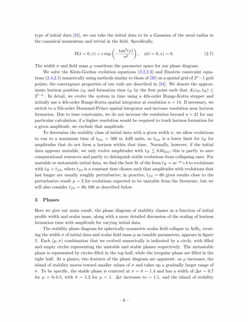
The width σ and field mass µ constitute the parameter space for our phase diagram.
We solve the Klein-Gordon evolution equations (2.2,2.3) and Einstein constraint equa-
tions (2.4,2.5) numerically using methods similar to those of [20] on a spatial grid of 2n−1 grid
points; the convergence properties of our code are described in [34]. We denote the approx-
imate horizon position xH and formation time tH by the first point such that A(xH , tH) ≤27−n. In detail, we evolve the system in time using a 4th-order Runge-Kutta stepper and
initially use a 4th-order Runge-Kutta spatial integrator at resolution n = 14. If necessary, we
switch to a 5th-order Dormand-Prince spatial integrator and increase resolution near horizon
formation. Due to time constraints, we do not increase the resolution beyond n = 21 for any
particular calculation; if a higher resolution would be required to track horizon formation for
a given amplitude, we exclude that amplitude.
To determine the stability class of initial data with a given width σ, we allow evolutions
to run to a maximum time of tlim = 500 in AdS units, so tlim is a lower limit for tH for
amplitudes that do not form a horizon within that time. Normally, however, if the initial
data appears unstable, we only evolve amplitudes with tH . 0.6tlim; this is partly to save
computational resources and partly to distinguish stable evolutions from collapsing ones. For
unstable or metastable initial data, we find the best fit of the form tH = aε−p+b to evolutions
with tH > tfit, where tfit is a constant time chosen such that amplitudes with evolutions that
last longer are usually roughly perturbative; in practice, tfit = 60 gives results close to the
perturbative result p = 2 for evolutions expected to be unstable from the literature, but we
will also consider tfit = 80, 100 as described below.
3 Phases
Here we give our main result, the phase diagram of stability classes as a function of initial
profile width and scalar mass, along with a more detailed discussion of the scaling of horizon
formation time with amplitude for varying initial data.
The stability phase diagram for spherically symmetric scalar field collapse in AdS5, treat-
ing the width σ of initial data and scalar field mass µ as tunable parameters, appears in figure
2. Each (µ, σ) combination that we evolved numerically is indicated by a circle, with filled
and empty circles representing the unstable and stable phases respectively. The metastable
phase is represented by circles filled in the top half, while the irregular phase are filled in the
right half. At a glance, two features of the phase diagram are apparent: as µ increases, the
island of stability moves toward smaller values of σ and takes up a gradually larger range of
σ. To be specific, the stable phase is centered at σ = σ ∼ 1.4 and has a width of ∆σ ∼ 0.7
for µ = 0, 0.5, with σ ∼ 1.2 for µ = 1. ∆σ increases to ∼ 1.1, and the island of stability
– 6 –

0 1 2 3 4
σ
0
5
10
15
20
µ
Figure 2: Phase diagram as a function of initial data width σ and scalar mass µ. Filled
circles represent the unstable phase, empty circles the stable phase, top-half-filled circles
metastability, and right-half-filled circles the irregular phase.
is centered at σ ∼ 0.9 for µ = 5, 10, while ∆σ ∼ 1.2 for µ = 15, 20 with the stable phase
centered at σ ∼ 0.8. Note that the transition between “light field” and “heavy field” behavior
occurs for µ > 1 in AdS units.
The metastable and irregular phases appear at the shorelines of the island of stability,
the boundary between unstable and stable phases. In particular, the slope of the power law
tH ∼ ε−p as ε → 0 increases as the width moves toward the island of stability, leading to a
metastable phase. We find metastability at the large σ shoreline for all µ values considered
and also at the small σ shoreline for several scalar masses. It seems likely that metastable
behavior appears in only a narrow range of σ for larger µ, which makes it harder to detect in
a numerical search, leading to its absence in some parts of the phase diagram. We find the
irregular phase at the small σ shoreline for every mass and at the large σ boundary for large
µ, closer to stable values of σ than the metastable phase. This phase includes a variety of
irregular and non-monotonic behavior, as detailed below. Truly chaotic behavior especially
becomes more prominent at larger values of µ, as we will discuss below.
3.1 Metastable versus unstable phases
While the stable and irregular phases are typically apparent by eye in a plot of tH vs ε,
distinguishing the unstable from metastable phase is a quantitative task. As we described in
section 2.2, we find the least squares fit of tH = aε−p + b to all evolutions with tH > tfit for
the given (µ, σ), running over values tfit = 60, 80, 100. Using the covariance matrix of the fit,
we also find the standard error for each fit parameter. We classify a width as having unstable
evolution if the best fit value of p is within two standard errors of p = 2 for tfit = 60, 80
or one standard error for tfit = 100 (due to a smaller number of data points, the standard
errors for tfit = 100 tend to be considerably larger).1 Considering larger values of tfit helps
1except for poor fits as described in our discussion of the irregular phase.
– 7 –

0.1 0.2 0.3 0.4 0.5 0.6 0.70
2000
4000
6000
8000
10000
a
Figure 3: Coefficient a from the fit tH = aε−p + b as a function of width σ using tfit = 60.
Shows data for µ = 0 (green diamonds), 0.5 (red triangles), 1 (yellow stars), 5 (black circles),
10 (cyan squares), 15 (magenta Y), and 20 (blue circles). The orange line is the best power
law fit.
to ensure that the particular initial profile does not reach the perturbative regime at smaller
amplitude values.
The fits tH = aε−p + b allow us to explore the time scale of horizon formation across the
phase diagram, for example through a contour plot of one of the coefficients vs σ and µ. In
most cases, this has not been informative, but an intriguing feature emerges if we plot the
normalization coefficient a vs σ for unstable initial data at small σ, as shown in figure 3 for
tfit = 60. By eye, the coefficient is reasonably well described by the fit a = 32.0(3)σ−2.01(2)
(values in parentheses are standard errors of the best fit values) independent of scalar field
mass. This is not born out very well quantitatively; the reduced χ2 for the fit is χ2/d.o.f.= 180,
indicating a poor fit. However, the large χ2 seems largely driven by a few outlier points with
large scalar mass, so it is tempting to speculate that the gravitational collapse in this region of
parameter space is driven by gradient energy, making all fields effectively massless at narrow
enough initial σ. The picture is qualitatively similar if we consider the parameter a for
tfit = 80, 100 instead.
Several examples of metastable behavior appear in figure 4. These figures show both data
from the numerical evolutions (blue dots and red triangles) and fits of the form tH = aε−p+ b
for points with tH > tfit = 60 (magenta curves). The best fit parameters are given in table
1.
Figures 4a,4b demonstrate behavior typical of most of the instances of metastable initial
data we have found; specifically, the initial data continue to collapse through horizon for-
mation times of tH ∼ 0.6tlim but with p significantly greater than the perturbative value of
p = 2. Note that the evolutions of figure 4b have been extended to larger values of tH to
demonstrate that the evolutions continue to collapse to somewhat smaller amplitude values.
Figure 4b is also of interest because its best fit value p ≈ 2.08 is approximately as close to
– 8 –

0.0310 0.0648 0.0986 0.1324 0.1662 0.2000ε
0
100
200
300
400
500t H
(a) µ = 15, σ = 1.5
0.05 0.09 0.13 0.17 0.21 0.25
ε
0
100
200
300
400
500
t H
(b) µ = 5, σ = 1.7
0.110 0.248 0.386 0.524 0.662 0.800ε
0
100
200
300
400
500
t H
(c) µ = 0, σ = 1.8
0.1960 0.2368 0.2776 0.3184 0.3592 0.4000
ε
0
100
200
300
400
500
t H
(d) µ = 0.5, σ = 1.7
Figure 4: Metastable behavior: blue dots represent horizon formation and red triangles a
lower limit on tH . Magenta curves are fits tH = aε−p + b over the shown range of amplitudes.
See table 1 for best fit parameters.
the perturbative value as several stable sets of initial data but has a smaller standard error
for the fit, so the difference from the perturbative value is more significant.
Figure 4c shows metastable evolution to tH . 0.6tlim but then a sudden jump to stability
until t = tlim. In the figure, the fit has been extended to the largest non-collapsing amplitude,
which demonstrates that there is no collapse over a time period significantly longer than the fit
predicts. This example argues that metastable data may in fact become stable at the smallest
amplitudes. On the other hand, figure 4d shows a similar jump in tH to values tH < tlim;
evolution at lower amplitudes shows metastable scaling with p ≈ 6 for 360 < tH < tlim. The
figure also shows a metastable fit with larger reduced χ2 at larger amplitudes corresponding to
tfit < tH < 0.4tlim. So this is another option: metastable behavior may transition abruptly to
metastable behavior with different scaling (or possibly even perturbatively unstable behavior)
– 9 –

a p b χ2/d.o.f.
µ = 15, σ = 1.5 0.10(1) 2.33(5) -27(4) 0.7736
µ = 5, σ = 1.7 0.89(5) 2.08(2) -33(2) 0.3248
µ = 0, σ = 1.8 0.06(2) 4.3(2) 30(5) 1.502
µ = 0.5, σ = 1.7 (tH < 0.4tlim) 4(32)×10−45 73(5) 70(2) 5.409
(tH > 0.72tlim) 0.02(3) 5.6(8) 260(20) 1.078
Table 1: Best fit parameters for the cases shown in figure 4 restricting to tH > tfit = 60 and
as noted. Values in parentheses are standard errors in the last digit. χ2/d.o.f. is the reduced
χ2 value used as a measure of goodness-of-fit.
at sufficiently small amplitudes. It is also reasonable to classify this case as irregular due to
the sudden jump in tH ; we choose metastable due to the clean metastable behavior at low
amplitudes.
3.2 Behaviors of the irregular phase
We have found a variety of irregular behaviors at the transition between the metastable and
stable phases which we have classified together as the irregular phase; however, it may be
better to describe them as separate phases. The phase diagram 2 indicates that the irregular
phase extends along the “inland” side of the small σ shoreline and at least part of the large
σ shoreline of the island of stability. What is not clear from our evolutions up to now is
whether each type of behavior appears along the entire shoreline or if they appear in pockets
at different scalar field masses. Examples of each type of behavior that we have found appear
in figure 5.
The first type of irregular behavior, shown in figure 5a, is monotonic (tH increases with
decreasing ε as usual), but it is not well fit by a power law. In fact, this behavior would
classify as metastable by the criterion of section 3.1 in that the power law of the best fit
tH = aε−p + b is significantly different from p = 2, except for the fact that the reduced χ2
value for the fit is very large (greater than 10) and also that different fitting algorithms can
return significantly different fits, even though the data may appear to the eye like a smooth
power law. In any case, this type of behavior apparently indicates a breakdown of metastable
behavior and hints at the appearance of non-monotonicity. So far, our evolutions have not
demonstrated sudden jumps in tH typical of stability at low amplitudes, however.
Figure 5b exemplifies non-monotonic behavior in the irregular phase. This type of behav-
ior, which was noted already by [18], involves one or more sudden jumps in tH as ε decreases,
which may be followed by a sudden decrease in tH and then resumed smooth monotonic
increase in tH . There are suggestions that this type of initial data is stable at low amplitudes
due to the usual appearance of non-collapsing evolutions, but it is worth noting that these
amplitudes could instead experience another jump and decrease in tH , just at tH > tlim.
Finally, [34] studied this type of behavior in some detail, denoting it as “quasi-stable.”
– 10 –

0.960 1.168 1.376 1.584 1.792 2.000ε
0
100
200
300
400
500t H
(a) µ = 0.5, σ = 1
3.370 3.496 3.622 3.748 3.874 4.000ε
0
100
200
300
400
500
t H
(b) µ = 5, σ = 0.34
8.420 8.736 9.052 9.368 9.684 10.000ε
0
100
200
300
400
500
t H
(c) µ = 20, σ = 0.16
6.640 6.912 7.184 7.456 7.728 8.000ε
0
100
200
300
400
500
t H
(d) µ = 20, σ = 0.19
Figure 5: Irregular behavior: blue dots represent horizon formation and red triangles a lower
limit on tH .
The last type of irregular behavior is apparently chaotic, in that tH appears to be sensitive
to initial conditions (ie, value of amplitude) over some range of amplitudes. This type of
behavior appears over the range of masses (see figure 1d for a mild case for massless scalars),
but it is more common and more dramatic at larger µ. Figures 5c,5d represent the most
extreme chaotic behavior among the initial data that we studied with collapse at tH <
50 not very far separated from amplitudes that do not collapse for t < tlim along with
an unpredictable pattern of variation in tH . This type of chaotic behavior has been seen
previously in the collapse of transparent but gravitationally interacting thin shells in AdS
[39] as well as in the collapse of massless scalars in AdS5 Einstein-Gauss-Bonnet gravity
[30, 31]. In both cases, the chaotic behavior is hypothesized to be due to the transfer of
energy between two infalling shells, with horizon formation only proceeding when one shell is
sufficiently energetic. In the latter case, the extra scale of the theory (given by the coefficient
– 11 –

0 20 40 60 80 100 120 140 160 180t
0
50
100
150
200
250
300
350
400
450|R|
(a) Upper envelope of Ricci scalar at origin
0 20 40 60 80 100 120 140tmid
1.5
1.0
0.5
0.0
0.5
1.0
1.5
2.0
log
10|∆|
(b) log |∆| vs. tmid
Figure 6: Left: The upper envelope of the Ricci scalar for amplitudes ε1 = 3.50 (blue circles),
ε2 = 3.51 (red triangles), and ε3 = 3.52 (green squares) for µ = 5, σ = 0.34. Right: log(|∆12|)and best fit (blue circles and line) and log(|∆23|) and best fit (red squares and line), calculated
as a function of the midpoint tmid of the time interval.
of the Gauss-Bonnet term in the action) leads the single initial pulse of scalar matter to break
into two pulses.
We should therefore ask two questions: does this irregular behavior show evidence of true
chaos, and is a similar mechanism at work here? To quantify the presence of chaos, we examine
the difference in time evolution between similar initial conditions (nearby amplitudes), which
diverge exponentially in chaotic systems. Specifically, any quantity ∆ should satisfy |∆| ∝exp(λt) for Lyapunov coefficient λ. Our characteristic will be the upper envelope of the Ricci
scalar at the origin per light crossing time, R(t). We consider the chaotic behavior exhibited
by three states: a massless scalar of width σ = 1.1 (see figure 1d), a µ = 5 massive scalar of
width σ = 0.34, and a µ = 20 scalar of width σ = 0.19 (figure 5d).
Figure 6 details evidence for chaotic evolution in the µ = 5, σ = 0.34 case; figure 6a shows
our characteristic function R(t) for the amplitudes ε1 = 3.50, ε2 = 3.51, and ε3 = 3.52. By
eye, R shows noticeable differences after a long period of evolution. These are more apparent
in figure 6b, which shows the log of the differences ∆ab ≡ Rεa −Rεb , along with the best fits.
Although there is considerable noise — or oscillation around exponential growth — in the
differences (leading to R2 values ∼ 0.2, 0.26 for the fits), the average slope gives Lyapunov
coefficient λ = 0.007 (within the error bar of each slope), and each slope differs from zero by
more than 3 standard errors. One interesting point is that the tH vs ε curve in figure 5b does
not appear chaotic to the eye, even though it shows some of the mathematical signatures of
chaos at least for ε1 < ε < ε3, the amplitude values near the visible spike in tH .
The story is similar for the massless and µ = 20 cases we studied, which exhibit λ values
that differ from zero by at least 1.9 standard deviations; see table 2. This is a milder version
– 12 –

λ average λ
µ = 0, σ = 1.1 ∆12 0.011(6) 0.011
∆23 0.011(5)
µ = 5, σ = 0.34 ∆12 0.006(2) 0.007
∆23 0.007(2)
µ = 20, σ = 0.19 ∆12 0.046(9) 0.032
∆23 0.019(7)
Table 2: Best fit Lyapunov coefficients λ for adjacent amplitude pairs and average λ value
for each µ, σ system studied. The parenthetical value is the error in the last digit.
of the chaotic behavior noted by [30, 31, 39], especially for the µ = 5 case studied. To our
knowledge, this is the first evidence of chaos in the gravitational collapse of a massless scalar
in AdS. One thing to note is that the strength of oscillation in log(|∆|) around the linear fit
increases with increasing mass, so that the two best fit Lyapunov exponents for µ = 20 are
no longer consistent with each other at the 1-standard deviation level.
The mechanism underlying the chaotic behavior seems somewhat different or at least
weaker than the two-shell or Einstein-Gauss-Bonnet systems. When examining the time
evolution of the mass distributions of these data, we see a single large pulse of mass energy that
oscillates between the origin and boundary without developing a pronounced peak. However,
there is also apparently a smaller wave that travels across the large peak. In the massless case
examined, this wave deforms the pulse, leading at times to the double-shoulder appearance
of figure 7a. In the µ = 5, σ = 0.34 case, the secondary wave is more like a ripple, usually
smaller in amplitude but more sharply localized, as toward the right side of the main pulse
in figure 7b. So the chaotic behavior may be caused by the relative motion of the two waves,
rather than energy transfer between two shells. In this hypothesis, a horizon would form
when both waves reach the neighborhood of the origin at the same time.
– 13 –

x0 0.2 0.4 0.6 0.8 1 1.2 1.4
M'
0
0.01
0.02
0.03
0.04
0.05
0.06
0.07
(a) µ = 0, σ = 1.1, ε = 1.01, t = 60
x0 0.2 0.4 0.6 0.8 1 1.2 1.4
M'
0
0.002
0.004
0.006
0.008
0.01
0.012
0.014
0.016
0.018
0.02
(b) µ = 5, σ = 0.34, ε = 3.52, t = 137
Figure 7: Radial derivative of the mass function at the indicated time for two chaotic
systems. Note the appearance of a secondary wave on top of the main pulse. (µ, σ, ε) as
indicated.
4 Spectral analysis
As we discussed in the introduction, instability toward horizon formation proceeds through a
turbulent cascade of energy to shorter wavelengths or, more quantitatively, to 1st-order scalar
eigenmodes with more nodes. Inverse cascades are typical of stable evolutions. Therefore,
understanding the energy spectrum of our evolutions, both initially and over time, sheds light
on the behavior of the self-gravitating scalar field in asymptotically AdS spacetime.
The (normalizable) eigenmodes ej are given by Jacobi polynomials as
ej(x) = κj cosλ+(x)P(d/2−1,
√d2+4µ2/2)
j (cos(2x)) (4.1)
(κj is a normalization constant) with eigenfrequency ωj = 2j+λ+ and λ+ = (d+√d2 + 4µ2)/2
in AdSd+1 for j = 0, 1, · · · (see [40, 41] for reviews). Including gravitational backreaction, we
define the energy spectrum
Ej ≡1
2
(Πj
2 − φjφj), (4.2)
where
Πj =(√
AΠ, ej
), φj = (φ, ej) ,
φj =(
cotd−1(x)∂x
[tand−1(x)AΦ
]− µ2 sec2(x)φ, ej
), (4.3)
and the inner product is (f, g) =∫ π/20 dx tand−1(x)fg. The sum of Ej over all modes is the
conserved ADM mass.
4.1 Dependence on mass
The most visibly apparent feature of the phase diagram of figure 2 is that the island of stability
both expands and shifts to smaller widths as the scalar mass increases. As it turns out, the
energy spectrum of the Gaussian initial data (2.7) provides a simple heuristic explanation.
– 14 –

1 2 3 4 5 6 7 8 9 1011121310-14
10-11
10-8
10-5
10-2
j
Ej/M
ADM
(a) Best fit gaussian energy spectra.
0.0 0.5 1.0 1.5
0
5
10
15
20
25
30
x
Π(x),e 0
(x)
(b) Best fit gaussian and zeroth eigenmode.
Figure 8: Left: Spectra of the best fit gaussians (2.7) to the j = 0 eigenmode for masses
µ = 0 (blue circles), 0.5 (yellow squares), 1 (empty orange circles), 5 (green diamonds), 10
(empty cyan squares), 15 (upward red triangles), and 20 (downward purple triangles). Right:
an overlay of the best fit Gaussian and e0 eigenmode for µ = 0 (solid blue is best fit, orange
dashed is eigenmode) and µ = 20 (solid green, red short dashes).
It is well established both in perturbation theory and numerical studies that initial data
given by a single scalar linear-order eigenmode is in fact nonlinearly stable, and the spectra
of many quasi-periodic solutions are also dominated by a single eigenmode. As a result, we
should expect Gaussian initial data that approximates a single eigenmode (which must be
j = 0 due to lack of nodes) to be stable. To explore how this depends on mass, we find the best
fit values of ε, σ for the j = 0 eigenmode for each mass that we consider (defined by the least-
square error from the Gaussian to a discretized eigenmode); this is the “best approximation”
Gaussian to the eigenmode. Then we find the energy spectrum of that best-fit Gaussian;
these are shown in figure 8a. From the figure, it is clear that the j = 0 eigenmode is closer
to a Gaussian at larger masses. That is, other eigenmodes contribute less to the Gaussian’s
spectrum at higher masses (by several orders of magnitude over the range from µ = 0 to 20).
Simply put, the shape of the j = 0 eigenmode is closer to Gaussian at higher masses, which
suggests that the island of stability should be larger at larger scalar field mass. Figure 8b
compares the j = 0 eigenmode and best fit Gaussian for µ = 0 and 20; on inspection, there
is more deviation between the eigenmode and Gaussian for the massless scalar.
In addition, the best-fit Gaussian width decreases from σ ∼ 0.8 for a massless scalar as
the mass increases. At µ = 20, the best-fit width is σ ∼ 0.31. This suggests that Gaussians
that approximate the j = 0 mode well enough are narrower in width at higher masses. An
interesting point to note is that the island of stability for µ = 0, 0.5 is actually centered
at considerably larger widths than the best-fit Gaussian. This may not be surprising, since
the best-fit Gaussians at low masses actually receive non-negligible contributions from higher
mode numbers; moving away from the best-fit Gaussian can actually reduce the power in
higher modes. For example, the stable initial data shown in figure 9a below has considerably
less power in the j = 2 mode.
– 15 –

j10 210 310
AD
M/M j
E
14−10
13−10
12−10
11−10
10−10
9−10
8−10
7−10
6−10
5−10
4−10
3−10
2−10
1−10
(a) µ = 0, σ = 1.5
j10 210 310
AD
M/M j
E
14−10
13−10
12−10
11−10
10−10
9−10
8−10
7−10
6−10
5−10
4−10
3−10
2−10
1−10
(b) µ = 0, σ = 0.25
j10 210 310
AD
M/M j
E
14−10
13−10
12−10
11−10
10−10
9−10
8−10
7−10
6−10
5−10
4−10
3−10
2−10
1−10
(c) µ = 5, σ = 1.7
j10 210 310
AD
M/M j
E
14−10
13−10
12−10
11−10
10−10
9−10
8−10
7−10
6−10
5−10
4−10
3−10
2−10
1−10
(d) µ = 0.5, σ = 1
j10 210 310
AD
M/M j
E
14−10
13−10
12−10
11−10
10−10
9−10
8−10
7−10
6−10
5−10
4−10
3−10
2−10
1−10
(e) µ = 5, σ = 0.34
j10 210 310
AD
M/M j
E
14−10
13−10
12−10
11−10
10−10
9−10
8−10
7−10
6−10
5−10
4−10
3−10
2−10
1−10
(f) µ = 20, σ = 0.16
Figure 9: Initial (t = 0) energy spectra for the indicated evolutions. In order, these repre-
sent stable, unstable, metastable, monotonic irregular, non-monotonic irregular, and chaotic
irregular initial data.
4.2 Spectra of different phases
A key question that one might hope to answer is whether the stability phase of a given (µ, σ)
can be determined easily by direct inspection of the initial data without requiring many
evolutions at varying amplitudes. The initial energy spectra for examples of each phase,
including monotonic, non-monotonic, and chaotic irregular behaviors, are shown in figure 9.
These spectra are taken from among the smallest amplitudes we evolved in order to minimize
backreaction effects.
Unfortunately, the initial energy spectra do not seem to provide such a method for deter-
mining the stability phase. Very broadly speaking, stable and metastable (µ, σ) correspond to
initial spectra that drop off fairly quickly from the j = 0 mode as j increases, while unstable
and irregular phases tend to have roughly constant or even slightly increasing spectra up to
j = 5 or 10. However, figure 9d shows that some irregular initial data have spectra that
decrease rapidly after a small increase from j = 1 to j = 2. Kinks in the spectrum are more
prevalent for widths of the AdS scale or larger, while spectra for smaller widths tend to be
smoother.
4.3 Evolution of spectra
While the initial spectrum for a given (µ, σ) pair does not have predictive value regarding the
future behavior as far as we can tell, the time dependence of the spectrum throughout the
evolution of the system is informative. Figure 10 shows the time-dependence of spectra for
examples of the stable, unstable, metastable, and chaotic irregular phases. In each figure, the
– 16 –
0.0
0.2
0.4
0.6
0.8
1.0
Σj(E
j/M
AD
M)
0 100 200 300 400 500t
0.0
0.1
0.2
0.3
0.4
0.5
0.6
0.7
0.8
Ej/M
AD
M
(a) µ = 0, σ = 1.8, ε = 0.13
0.0
0.2
0.4
0.6
0.8
1.0
Σj(E
j/M
AD
M)
0 10 20 30 40 50 60 70t
0.00
0.05
0.10
0.15
0.20
0.25
0.30
Ej/M
AD
M
(b) µ = 0, σ = 0.25, ε = 2.28
0.0
0.2
0.4
0.6
0.8
1.0
Σj(E
j/M
AD
M)
0 50 100 150 200 250 300 350t
0.0
0.2
0.4
0.6
0.8
Ej/M
AD
M
(c) µ = 0.5, σ = 1.7, ε = 0.216
0.0
0.2
0.4
0.6
0.8
1.0
Σj(E
j/M
AD
M)
0 10 20 30 40 50 60t
0.0
0.1
0.2
0.3
0.4
Ej/M
AD
M
(d) µ = 20, σ = 0.19, ε = 6.95
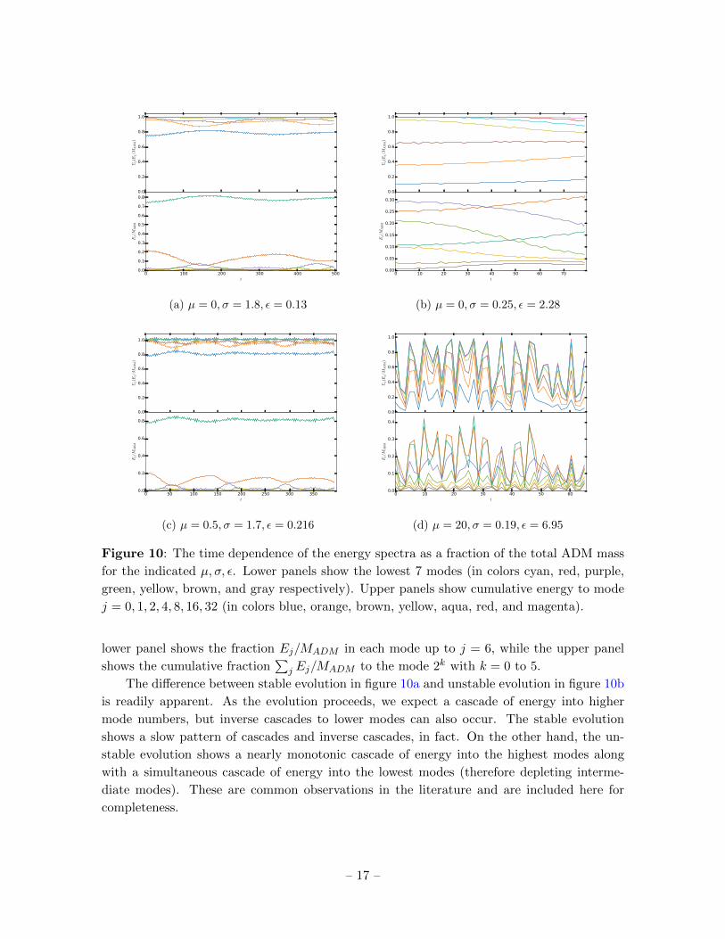
Figure 10: The time dependence of the energy spectra as a fraction of the total ADM mass
for the indicated µ, σ, ε. Lower panels show the lowest 7 modes (in colors cyan, red, purple,
green, yellow, brown, and gray respectively). Upper panels show cumulative energy to mode
j = 0, 1, 2, 4, 8, 16, 32 (in colors blue, orange, brown, yellow, aqua, red, and magenta).
lower panel shows the fraction Ej/MADM in each mode up to j = 6, while the upper panel
shows the cumulative fraction∑
j Ej/MADM to the mode 2k with k = 0 to 5.
The difference between stable evolution in figure 10a and unstable evolution in figure 10b
is readily apparent. As the evolution proceeds, we expect a cascade of energy into higher
mode numbers, but inverse cascades to lower modes can also occur. The stable evolution
shows a slow pattern of cascades and inverse cascades, in fact. On the other hand, the un-
stable evolution shows a nearly monotonic cascade of energy into the highest modes along
with a simultaneous cascade of energy into the lowest modes (therefore depleting interme-
diate modes). These are common observations in the literature and are included here for
completeness.
– 17 –

j10 210 310
AD
M/M j
E
14−10
13−10
12−10
11−10
10−10
9−10
8−10
7−10
6−10
5−10
4−10
3−10
2−10
1−10
(a) ε = 1.01
j10 210 310
AD
M/M j
E
14−10
13−10
12−10
11−10
10−10
9−10
8−10
7−10
6−10
5−10
4−10
3−10
2−10
1−10
(b) ε = 1.02
Figure 11: Spectra at time t ≈ 71 for µ = 0, σ = 1.1 for the two amplitudes given. ε = 1.1
forms a horizon at tH ≈ 71.1, ε = 1.02 at tH ≈ 248.0.
The metastable evolution shown in figure 10c is interesting in light of the stable and
unstable spectra. The amplitude shown is from the “unstable” portion of figure 4d, the part
consistent with the perturbative scaling tH ∼ ε−2. However, the spectrum shows a similar
pattern of slow cascades and inverse cascades to the stable phase example, though on a
somewhat faster time scale in this case. While perhaps surprising, this is in keeping with
the similarities noted between the initial spectra in figures 9a and 9c. We have also checked
that the time-dependent spectrum at a higher amplitude with tH ∼ 100 follows the same
pattern as 10c; in fact, it looks essentially the same but simply ends at an earlier time. This
lends some credence to the idea that the metastable phase is stable at lowest nontrivial order
in perturbation theory, with instability triggered by higher-order corrections. Alternately,
the instability could be caused by an oscillatory singularity in the perturbative theory, as
discussed in [15, 23–25] in the case of two-mode initial data. These divergences do not appear
in the energy spectrum.
Figure 10d shows the time-dependence of the spectrum in a chaotic irregular evolution,
specifically µ = 20, σ = 0.19 at ε = 6.95, which is in the chaotic region of the tH vs ε plot
in figure 5d. There is rapid energy transfer among modes, including cascades out of and
inverse cascades into mode numbers j ≤ 32 over approximately a light-crossing time. It is
easy to imagine that horizon formation might occur at any of the cascades of energy into
higher modes, leading to seemingly random jumps in tH as a function of amplitude.
Finally, the time-evolved energy provide another possible measure of approximate ther-
malization in the dual CFT; namely, the spectrum should approach an (exponentially cut-off)
power law at thermalization. In most cases, this occurs shortly before horizon formation, but
there are exceptions, such as the late time behavior of initial data below the critical mass for
black hole formation in Einstein-Gauss-Bonnet gravity [30]. In the case of chaotic behavior,
it is particularly interesting to know if the spectra for similar amplitudes approach a power
law at similar times even if horizons form at very different times. Figure 11 shows the en-
ergy spectra for two amplitudes in the chaotic region of the tH vs ε plot for µ = 0, σ = 1.1.
– 18 –

Figure 11a is the spectrum just before horizon formation for ε = 1.01, while figure 11b is
the spectrum at approximately the same time for ε = 1.02, which is very long before horizon
formation. In this example, we see that the spectrum does approach a power law for the
evolution that is forming a horizon, while the other evolution demonstrates apparently expo-
nential decay. Therefore, this example suggests that a power law spectrum may yield similar
results to horizon formation as a measure of thermalization in the dual CFT.
5 Discussion
We have presented the phase diagram of stability of AdS5 against horizon formation, treat-
ing the scalar field mass µ and width σ of initial data as free parameters. In addition to
mapping the location of the so-called “island of stability,” we have gathered evidence for
two non-perturbative phases on the “shorelines” of the island, the metastable and irregular
phases. While these must either exhibit stability (no collapse below some critical amplitude)
or instability (collapse at arbitrarily small but finite amplitude) as the amplitude ε → 0,
they are distinguished by their behavior at computationally accessible amplitudes. While
perturbatively unstable evolutions obey tH ∝ ε−2 as ε → 0, metastable initial data follows
tH ∝ ε−p for p > 2 over a range of amplitudes. The irregular phase is characterized by
horizon formation times tH that are not well described by a power law and sometimes exhibit
non-monotonicity or even chaos. Both of these phases appear across the range of µ values
that we study and at both small- and large-width boundaries of the stable phase.
At this time, it is impossible to say whether metastable initial data is stable or unstable
as ε → 0 (or if all metastable data behaves in the same way in that limit). Our numerical
evolutions include cases in which the lowest amplitudes jump either to metastable scaling
with smaller p or to evolutions that do not collapse over the timescales we study. In many
cases, too, the power law tH ∝ ε−p with p some fixed value > 2 is robust as we exclude larger
amplitudes from our fit. It is also possible that some of the metastable phase is stable in the
perturbative theory (ie, to ε3 order in a perturbative expansion) but not at higher orders.
The irregular phase seems likely to be (mostly) stable at arbitrarily small amplitudes
based on our numerical evolutions, though we have not found a critical amplitude for mono-
tonic irregular initial data. The irregular phase includes the “quasi-stable” initial data de-
scribed in [18, 34], which has a sudden increase then decrease in tH as ε decreases as well
as truly chaotic behavior. In fact, we have found evidence for weakly chaotic behavior at
the jump in tH for non-monotonic initial data in the form of a small but nonzero Lyapunov
coefficient. Both non-monotonicity and chaos become stronger and more common at larger
scalar masses; however, we have also found chaotic behavior for the massless scalar. To our
knowledge, this is the first evidence of chaos in spherically symmetric massless scalar collapse
in AdS, which is particularly interesting because there is only one physically meaningful ratio
of scales, σ as measured in AdS units.
Aside from the ultimate stability or instability of the metastable and irregular phases,
several questions remain. For one, black holes formed in massive scalar collapse in asymptoti-
– 19 –

cally flat spacetime exhibit a mass gap for initial profiles wider than the Compton wavelength
1/µ [42]. Whether this mass gap exists in AdS is not clear, and it may disappear through re-
peated gravitational focusing as the field oscillates many times across AdS; investigating this
type of critical behavior will likely require techniques similar to those of [43]. Returning to
our phase diagram, the physical mechanism responsible for chaos in the irregular phase is not
yet clear. Is it some generalization of the same mechanism as found in the two-shell system?
Also, would an alternate definition of approximate thermalization in the dual CFT, such as
development of a power-law spectrum, lead to a different picture of the phase diagram? Fi-
nally, the big question is whether there is some test that could be performed on initial data
alone that would predict in advance its phase? So far, no test is entirely successful, so new
ideas are necessary.
Acknowledgments
We would like to thank Brayden Yarish for help submitting jobs for the µ = 10 evolutions.
The work of ND is supported in part by a Natural Sciences and Engineering Research Council
of Canada PGS-D grant to ND, NSF Grant PHY-1606654 at Cornell University, and by a
grant from the Sherman Fairchild Foundation. The work of BC and AF is supported by
the Natural Sciences and Engineering Research Council of Canada Discovery Grant program.
This research was enabled in part by support provided by WestGrid (www.westgrid.ca) and
Compute Canada Calcul Canada (www.computecanada.ca).
References
[1] P. Bizon and A. Rostworowski, On weakly turbulent instability of anti-de Sitter space, Phys.
Rev. Lett. 107 (2011) 031102, [arXiv:1104.3702].
[2] D. Garfinkle and L. A. Pando Zayas, Rapid Thermalization in Field Theory from Gravitational
Collapse, Phys. Rev. D84 (2011) 066006, [arXiv:1106.2339].
[3] J. Jalmuzna, A. Rostworowski, and P. Bizon, A Comment on AdS collapse of a scalar field in
higher dimensions, Phys. Rev. D84 (2011) 085021, [arXiv:1108.4539].
[4] D. Garfinkle, L. A. Pando Zayas, and D. Reichmann, On Field Theory Thermalization from
Gravitational Collapse, JHEP 02 (2012) 119, [arXiv:1110.5823].
[5] O. J. C. Dias, G. T. Horowitz, and J. E. Santos, Gravitational Turbulent Instability of Anti-de
Sitter Space, Class. Quant. Grav. 29 (2012) 194002, [arXiv:1109.1825].
[6] V. Balasubramanian, A. Buchel, S. R. Green, L. Lehner, and S. L. Liebling, Holographic
Thermalization, Stability of Anti–de Sitter Space, and the Fermi-Pasta-Ulam Paradox, Phys.
Rev. Lett. 113 (2014), no. 7 071601, [arXiv:1403.6471].
[7] B. Craps, O. Evnin, and J. Vanhoof, Renormalization group, secular term resummation and
AdS (in)stability, JHEP 10 (2014) 048, [arXiv:1407.6273].
[8] P. Basu, C. Krishnan, and A. Saurabh, A stochasticity threshold in holography and the
instability of AdS, Int. J. Mod. Phys. A30 (2015), no. 21 1550128, [arXiv:1408.0624].
– 20 –

[9] F. V. Dimitrakopoulos, B. Freivogel, M. Lippert, and I.-S. Yang, Position space analysis of the
AdS (in)stability problem, JHEP 08 (2015) 077, [arXiv:1410.1880].
[10] A. Buchel, S. R. Green, L. Lehner, and S. L. Liebling, Conserved quantities and dual turbulent
cascades in anti–de Sitter spacetime, Phys. Rev. D91 (2015), no. 6 064026, [arXiv:1412.4761].
[11] B. Craps, O. Evnin, and J. Vanhoof, Renormalization, averaging, conservation laws and AdS
(in)stability, JHEP 01 (2015) 108, [arXiv:1412.3249].
[12] O. Evnin and C. Krishnan, A Hidden Symmetry of AdS Resonances, Phys. Rev. D91 (2015),
no. 12 126010, [arXiv:1502.03749].
[13] F. Dimitrakopoulos and I.-S. Yang, Conditionally extended validity of perturbation theory:
Persistence of AdS stability islands, Phys. Rev. D92 (2015), no. 8 083013, [arXiv:1507.02684].
[14] S. R. Green, A. Maillard, L. Lehner, and S. L. Liebling, Islands of stability and recurrence times
in AdS, Phys. Rev. D92 (2015), no. 8 084001, [arXiv:1507.08261].
[15] B. Craps, O. Evnin, and J. Vanhoof, Ultraviolet asymptotics and singular dynamics of AdS
perturbations, JHEP 10 (2015) 079, [arXiv:1508.04943].
[16] B. Craps, O. Evnin, P. Jai-akson, and J. Vanhoof, Ultraviolet asymptotics for quasiperiodic
AdS4 perturbations, JHEP 10 (2015) 080, [arXiv:1508.05474].
[17] B. Craps and O. Evnin, AdS (in)stability: an analytic approach, Fortsch. Phys. 64 (2016)
336–344, [arXiv:1510.07836].
[18] A. Buchel, S. L. Liebling, and L. Lehner, Boson stars in AdS spacetime, Phys. Rev. D87
(2013), no. 12 123006, [arXiv:1304.4166].
[19] M. Maliborski and A. Rostworowski, A comment on ”Boson stars in AdS”, arXiv:1307.2875.
[20] M. Maliborski and A. Rostworowski, Lecture Notes on Turbulent Instability of Anti-de Sitter
Spacetime, Int. J. Mod. Phys. A28 (2013) 1340020, [arXiv:1308.1235].
[21] P. Bizon and A. Rostworowski, Comment on “Holographic Thermalization, Stability of Anti–de
Sitter Space, and the Fermi-Pasta-Ulam Paradox”, Phys. Rev. Lett. 115 (2015), no. 4 049101,
[arXiv:1410.2631].
[22] V. Balasubramanian, A. Buchel, S. R. Green, L. Lehner, and S. L. Liebling, Reply to Comment
on “Holographic Thermalization, Stability of Anti–de Sitter Space, and the Fermi-Pasta-Ulam
Paradox”, Phys. Rev. Lett. 115 (2015), no. 4 049102, [arXiv:1506.07907].
[23] P. Bizon, M. Maliborski, and A. Rostworowski, Resonant Dynamics and the Instability of
Anti–de Sitter Spacetime, Phys. Rev. Lett. 115 (2015), no. 8 081103, [arXiv:1506.03519].
[24] N. Deppe, On the stability of anti-de Sitter spacetime, arXiv:1606.02712.
[25] F. V. Dimitrakopoulos, B. Freivogel, J. F. Pedraza, and I.-S. Yang, Gauge dependence of the
AdS instability problem, Phys. Rev. D94 (2016), no. 12 124008, [arXiv:1607.08094].
[26] F. V. Dimitrakopoulos, B. Freivogel, and J. F. Pedraza, Fast and Slow Coherent Cascades in
Anti-de Sitter Spacetime, arXiv:1612.04758.
[27] S. L. Liebling and G. Khanna, Scalar collapse in AdS with an OpenCL open source code,
arXiv:1706.07413.
– 21 –

[28] P. Bizon and J. Ja lmuzna, Globally regular instability of AdS3, Phys. Rev. Lett. 111 (2013),
no. 4 041102, [arXiv:1306.0317].
[29] E. da Silva, E. Lopez, J. Mas, and A. Serantes, Collapse and Revival in Holographic Quenches,
JHEP 04 (2015) 038, [arXiv:1412.6002].
[30] N. Deppe, A. Kolly, A. R. Frey, and G. Kunstatter, Black Hole Formation in AdS
Einstein-Gauss-Bonnet Gravity, JHEP 10 (2016) 087, [arXiv:1608.05402].
[31] N. Deppe, A. Kolly, A. Frey, and G. Kunstatter, Stability of AdS in Einstein Gauss Bonnet
Gravity, Phys. Rev. Lett. 114 (2015) 071102, [arXiv:1410.1869].
[32] R. Arias, J. Mas, and A. Serantes, Stability of charged global AdS4 spacetimes, JHEP 09 (2016)
024, [arXiv:1606.00830].
[33] H. Okawa, J. C. Lopes, and V. Cardoso, Collapse of massive fields in anti-de Sitter spacetime,
arXiv:1504.05203.
[34] N. Deppe and A. R. Frey, Classes of Stable Initial Data for Massless and Massive Scalars in
Anti-de Sitter Spacetime, JHEP 12 (2015) 004, [arXiv:1508.02709].
[35] V. E. Hubeny and M. Rangamani, Unstable horizons, JHEP 05 (2002) 027, [hep-th/0202189].
[36] A. Buchel and L. Lehner, Small black holes in AdS5 × S5, Class. Quant. Grav. 32 (2015),
no. 14 145003, [arXiv:1502.01574].
[37] A. Buchel, Universality of small black hole instability in AdS/CFT, arXiv:1509.07780.
[38] A. Buchel and M. Buchel, On stability of nonthermal states in strongly coupled gauge theories,
arXiv:1509.00774.
[39] R. Brito, V. Cardoso, and J. V. Rocha, Interacting shells in AdS spacetime and chaos, Phys.
Rev. D94 (2016), no. 2 024003, [arXiv:1602.03535].
[40] O. Aharony, S. S. Gubser, J. M. Maldacena, H. Ooguri, and Y. Oz, Large N field theories,
string theory and gravity, Phys. Rept. 323 (2000) 183–386, [hep-th/9905111].
[41] H. Nastase, Introduction to the ADS/CFT Correspondence. Cambridge University Press, 2015.
[42] P. R. Brady, C. M. Chambers, and S. M. C. V. Goncalves, Phases of massive scalar field
collapse, Phys. Rev. D56 (1997) 6057–6061, [gr-qc/9709014].
[43] D. Santos-Olivan and C. F. Sopuerta, Moving closer to the collapse of a massless scalar field in
spherically symmetric anti–de Sitter spacetimes, Phys. Rev. D93 (2016), no. 10 104002,
[arXiv:1603.03613].
– 22 –