phar 7633 chapter 15 multiple oral dose administration · did for an iv multiple dose regimen. ......
TRANSCRIPT
2/12/14, 7:01 PMc15
Page 1 of 15http://www.boomer.org/c/p4/c15/c15.html
PHAR 7633 Chapter 15
Multiple Oral Dose Administration
Multiple Oral Dose Administration
Student Objectives for this Chapter
After completing the material in this chapter each student should:-
be able to use the integrated equations for multiple oral dose administration to calculate plasma concentration orcalculate appropriate multiple dose regimenbe able to define, use, and calculate the parameter:
average plasma concentration,
be able to use the equation to calculate or adjust an appropriate dosing regimen
be able to use the superposition principle to calculate Cp after non uniform IV or oral dosing regimen
This page was last modified: Wednesday 26 May 2010 at 08:58 AM
Material on this website should be used for Educational or Self-Study Purposes Only
Copyright © 2001-2014 David W. A. Bourne ([email protected])
2/12/14, 7:01 PMc15
Page 2 of 15http://www.boomer.org/c/p4/c15/c15.html
PHAR 7633 Chapter 15
Multiple Oral Dose Administration
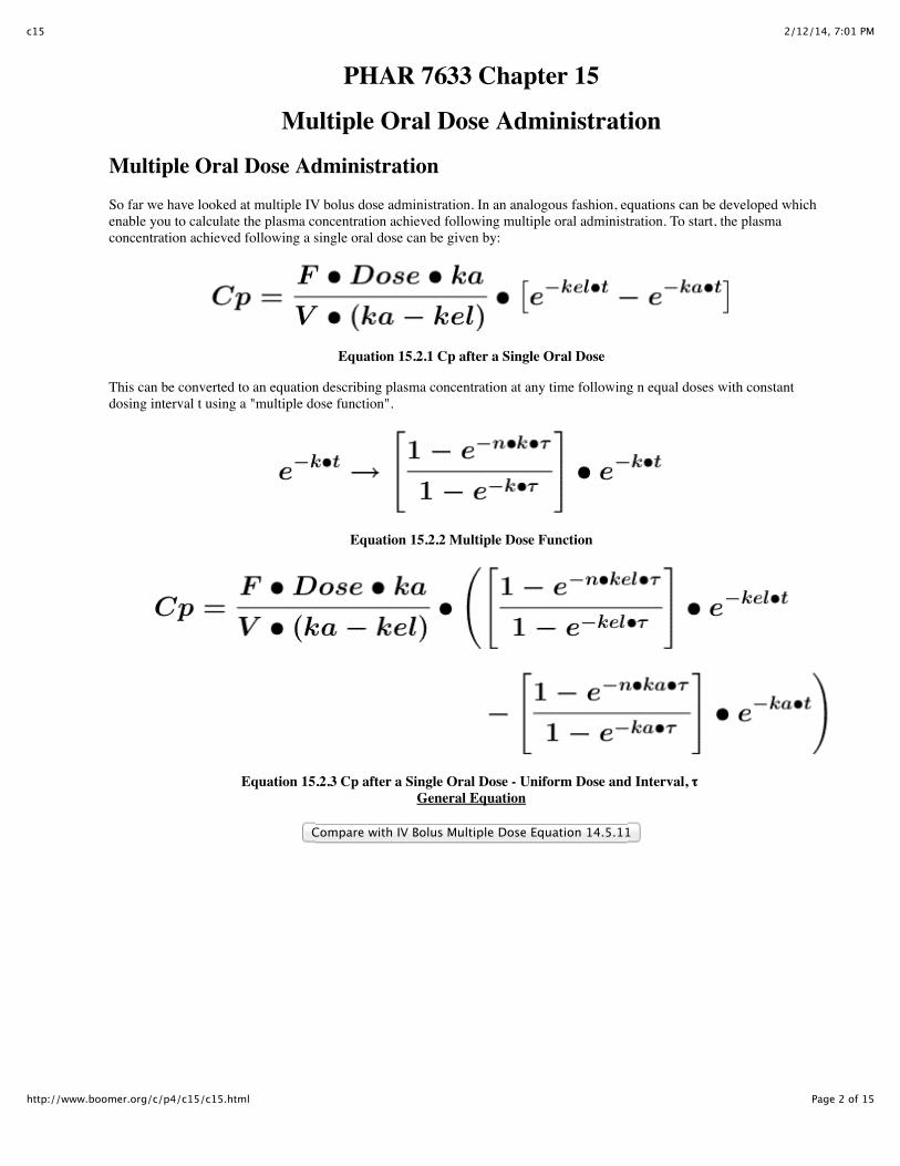
Multiple Oral Dose AdministrationSo far we have looked at multiple IV bolus dose administration. In an analogous fashion, equations can be developed whichenable you to calculate the plasma concentration achieved following multiple oral administration. To start, the plasmaconcentration achieved following a single oral dose can be given by:
Equation 15.2.1 Cp after a Single Oral Dose
This can be converted to an equation describing plasma concentration at any time following n equal doses with constantdosing interval t using a "multiple dose function".
Equation 15.2.2 Multiple Dose Function
Equation 15.2.3 Cp after a Single Oral Dose - Uniform Dose and Interval, τ General Equation
Compare with IV Bolus Multiple Dose Equation 14.5.11
2/12/14, 7:01 PMc15
Page 3 of 15http://www.boomer.org/c/p4/c15/c15.html
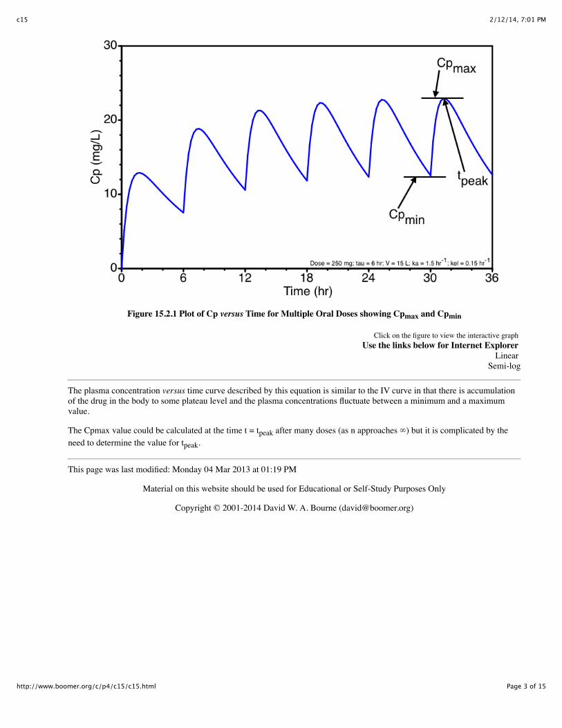
Figure 15.2.1 Plot of Cp versus Time for Multiple Oral Doses showing Cpmax and Cpmin
Click on the figure to view the interactive graph Use the links below for Internet Explorer
Linear Semi-log
The plasma concentration versus time curve described by this equation is similar to the IV curve in that there is accumulationof the drug in the body to some plateau level and the plasma concentrations fluctuate between a minimum and a maximumvalue.
The Cpmax value could be calculated at the time t = tpeak after many doses (as n approaches ∞) but it is complicated by theneed to determine the value for tpeak.
This page was last modified: Monday 04 Mar 2013 at 01:19 PM
Material on this website should be used for Educational or Self-Study Purposes Only
Copyright © 2001-2014 David W. A. Bourne ([email protected])
2/12/14, 7:01 PMc15
Page 4 of 15http://www.boomer.org/c/p4/c15/c15.html
PHAR 7633 Chapter 15
Multiple Oral Dose Administration
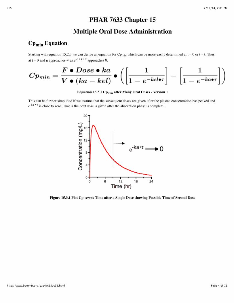
Cpmin Equation
Starting with equation 15.2.3 we can derive an equation for Cpmin which can be more easily determined at t = 0 or t = t. Thusat t = 0 and n approaches ∞ as e-n • k • τ approaches 0.
Equation 15.3.1 Cpmin after Many Oral Doses - Version 1
This can be further simplified if we assume that the subsequent doses are given after the plasma concentration has peaked ande-ka • τ is close to zero. That is the next dose is given after the absorption phase is complete.
Figure 15.3.1 Plot Cp versus Time after a Single Dose showing Possible Time of Second Dose

2/12/14, 7:01 PMc15
Page 5 of 15http://www.boomer.org/c/p4/c15/c15.html
Cpmin then becomes:
Equation 15.3.2 Cpmin after Many Oral Doses - Version 2
The relationship between loading dose and maintenance dose and thus drug accumulation during multiple dose administrationcan be studied by looking at the ratio between the minimum concentration at steady state and the concentration at the end ofthe first dosing interval,τ, after the first dose. [Assuming e-ka • τ is close to zero].
Equation 15.3.3 Ratio Between Cp after First and Last Dose
Which can be simplified to give:
Equation 15.3.4 Ratio Between Cp after First and Last Dose
This turns out to be the same equation as for the multiple IV bolus doses. Therefore we can estimate a loading dose just as wedid for an IV multiple dose regimen.
Equation 15.3.5 Loading Dose Equation
This equation holds if each dose is given after the absorption phase of the previous dose is complete.
We can further simplify Equation 15.3.2 when ka is high if we assume that ka >> kel then (ka - kel) is approximately equal toka and ka/(ka - kel) is approximately equal to one.
2/12/14, 7:01 PMc15
Page 6 of 15http://www.boomer.org/c/p4/c15/c15.html
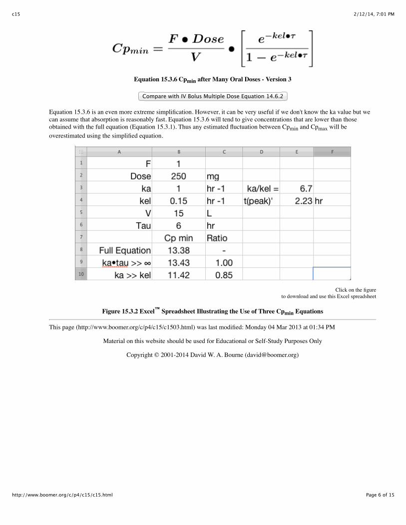
Equation 15.3.6 Cpmin after Many Oral Doses - Version 3
Compare with IV Bolus Multiple Dose Equation 14.6.2
Equation 15.3.6 is an even more extreme simplification. However, it can be very useful if we don't know the ka value but wecan assume that absorption is reasonably fast. Equation 15.3.6 will tend to give concentrations that are lower than thoseobtained with the full equation (Equation 15.3.1). Thus any estimated fluctuation between Cpmin and Cpmax will beoverestimated using the simplified equation.
Click on the figureto download and use this Excel spreadsheet
Figure 15.3.2 Excel™ Spreadsheet Illustrating the Use of Three Cpmin Equations
This page (http://www.boomer.org/c/p4/c15/c1503.html) was last modified: Monday 04 Mar 2013 at 01:34 PM
Material on this website should be used for Educational or Self-Study Purposes Only
Copyright © 2001-2014 David W. A. Bourne ([email protected])
2/12/14, 7:01 PMc15
Page 7 of 15http://www.boomer.org/c/p4/c15/c15.html
PHAR 7633 Chapter 15
Multiple Oral Dose Administration
Cpaverage Equation
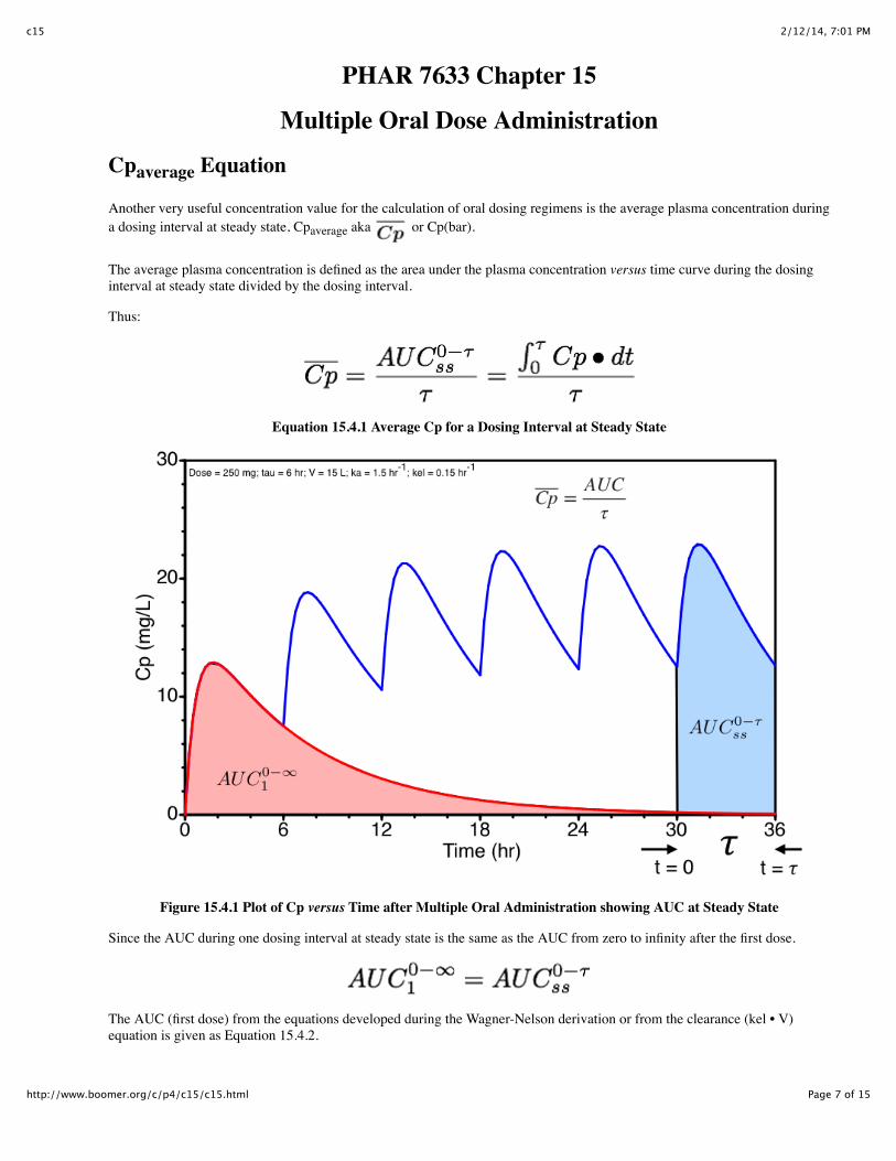
Another very useful concentration value for the calculation of oral dosing regimens is the average plasma concentration duringa dosing interval at steady state, Cpaverage aka or Cp(bar).
The average plasma concentration is defined as the area under the plasma concentration versus time curve during the dosinginterval at steady state divided by the dosing interval.
Thus:
Equation 15.4.1 Average Cp for a Dosing Interval at Steady State
Figure 15.4.1 Plot of Cp versus Time after Multiple Oral Administration showing AUC at Steady State
Since the AUC during one dosing interval at steady state is the same as the AUC from zero to infinity after the first dose.
The AUC (first dose) from the equations developed during the Wagner-Nelson derivation or from the clearance (kel • V)equation is given as Equation 15.4.2.
2/12/14, 7:01 PMc15
Page 8 of 15http://www.boomer.org/c/p4/c15/c15.html
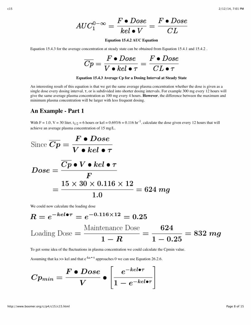
Equation 15.4.2 AUC Equation
Equation 15.4.3 for the average concentration at steady state can be obtained from Equation 15.4.1 and 15.4.2 .
Equation 15.4.3 Average Cp for a Dosing Interval at Steady State
An interesting result of this equation is that we get the same average plasma concentration whether the dose is given as asingle dose every dosing interval, τ, or is subdivided into shorter dosing intervals. For example 300 mg every 12 hours willgive the same average plasma concentration as 100 mg every 4 hours. However, the difference between the maximum andminimum plasma concentration will be larger with less frequent dosing.
An Example - Part 1
With F = 1.0, V = 30 liter, t1/2 = 6 hours or kel = 0.693/6 = 0.116 hr-1, calculate the dose given every 12 hours that willachieve an average plasma concentration of 15 mg/L.
We could now calculate the loading dose
To get some idea of the fluctuations in plasma concentration we could calculate the Cpmin value.
Assuming that ka >> kel and that e-ka • τ approaches 0 we can use Equation 26.2.6.

2/12/14, 7:01 PMc15
Page 9 of 15http://www.boomer.org/c/p4/c15/c15.html
Therefore the plasma concentration would probably fluctuate between 7 and 23 mg/L (very approximate) with an averageconcentration of about 15 mg/L. [23 = 15 + (15 - 7), i.e. high = average + (average - low), very approximate!].
An Example - Part 2As an alternative we could give half the dose, 312 mg, every 6 hours to achieve:
The would be the same
Thus the plasma concentration would fluctuate between about 10.4 to 20 with an average of 15 mg/L, Figure 15.4.2. The exactequation was used for the calculation in Figure 15.4.2.
Figure 15.4.2 Figure Illustrating Cpmax, Cpmin and Cp(average)
Some items to consider
2/12/14, 7:01 PMc15
Page 10 of 15http://www.boomer.org/c/p4/c15/c15.html
Item 1. Changing the dosing interval and the dose in the same proportion should produce the same Cpaverage concentration.However, the Cpmin and Cpmax can vary considerably.
With F = 1.0, V = 30 liter, t1/2 = 6 hours or kel = 0.693/6 = 0.116 hr-1, a dose of 600 mg given every 12 hours will achieve anaverage plasma concentration of approximately 15 mg/L. Try simulating this regimen and also the alternate regimen of 1200mg very 24 hours and 300 mg every 6 hours. Which regimen gives the least variation between Cpmax and Cpmin? Explore theproblem as a Plot - Interactive graph. (IE Version)
Item 2. Metabolism can be subject to a number of factors, such as genetics, disease state and co-administration of othercompounds. Other compounds may inhibit metabolism or induce metabolic activity. Some drugs are capable of inducing theirown metabolism.
Carbamazepine is a drug which can induce its own metabolism during the first few days of therapy (Hawkins Van Tyle andWinter, 2004). After the first dose, carbamazepine pharmacokinetic parameters include F = 0.8, V = 1.4 L/hr, CL = 0.028L/Kg/hr. After 3 to 5 days carbamazepine metabolism is induced such that the CL becomes 0.064 L/Kg/gr. For a 70 Kgpatients pre-induction (first-dose) parameter values are kel = 0.02 hr-1 and V = 100 L. After induction the kel changes to 0.045hr-1. Dose adjustment during the first few days can be difficult. Using post induction parameters for initial dosage regimencould cause toxic concentrations. For example, try the simulation again with a dose regimen of 600 mg every 12 hours withboth pre and post induction kel values. The typical therapeutic plasma concentration range is 4 - 12 mg/L. Explore theproblem as a Plot - Interactive graph. (IE Version)
Item 3. Theophylline has been studied extensively. It has been used commonly and has been the subject of therapeutic drugmonitoring (TDM) because of its variable pharmacokinetic parameters and narrow therapeutic window. Theophyllineparameter values vary considerably with disease state, enyzme status (drug co-administration or smoker status) andformulation factors. Currently, the therapeutic window ranges from 5 to 20 mg/L whereas earlier a range of 10 to 20 mg/L hadbeen used. Average plasma concentration targets includes values around 10 mg/L or in the range 8 to 15 mg/L (Aminimanizaniand Winter, 2004).
Theophylline is marketed in a number of oral dosage forms. Rapid release tablets generally are rapidly and completelyabsorbed with F close to 1.0 and ka values above 2 hr-1. The apparent volume of distribution is approximately 0.5 L/Kg (idealbody weight, IBW). Average values of theopylline clearance approximate 0.04 L/Kg/hr (based on IBW). A number of factorscan influence this average clearance value. For example; smoking x 1.6, cimetidine co-administration x 0.6, phenytoin co-administration 1.6, congestive heart failure x 0.5 (depending on status), cystic fibrosis x 1.5, hepatic cirrhosis x 0.5.Considering a 70 Kg (IBW) non-smoker patient the expected V and kel might be 35 L and 0.08 hr-1. For a patient that smokesthe kel would be expected to be approximately 0.125 hr-1. Try adjusting the parameter values according to these covariatesand adjust the dosing regimen to maintain appropriate therapeutic concentrations. Explore the problem as a Plot - Interactivegraph. (IE Version)
References
Hawkins Van Tyle, J. and Winter, M.E. 2004 Chapter 2 "Carbamazepine" in Basic Clinical Pharmacokinetics, 4thed., Winter, M.E., Lippincott Williams & Wilkins, Baltimore, MDAminimanizani, A. and Winter, M.E. 2004 Chapter 12 "Theophylline" in Basic Clinical Pharmacokinetics, 4th ed.,Winter, M.E., Lippincott Williams & Wilkins, Baltimore, MD
Practice problems involving Cpaverage, Cpmax and Cpmin at steady state after uniform multiple dose Oral doses.
This page (http://www.boomer.org/c/p4/c15/c1504.html) was last modified: Monday 04 Mar 2013 at 03:53 PM
Material on this website should be used for Educational or Self-Study Purposes Only
Copyright © 2001-2014 David W. A. Bourne ([email protected])
2/12/14, 7:01 PMc15
Page 11 of 15http://www.boomer.org/c/p4/c15/c15.html
PHAR 7633 Chapter 15
Multiple Oral Dose Administration
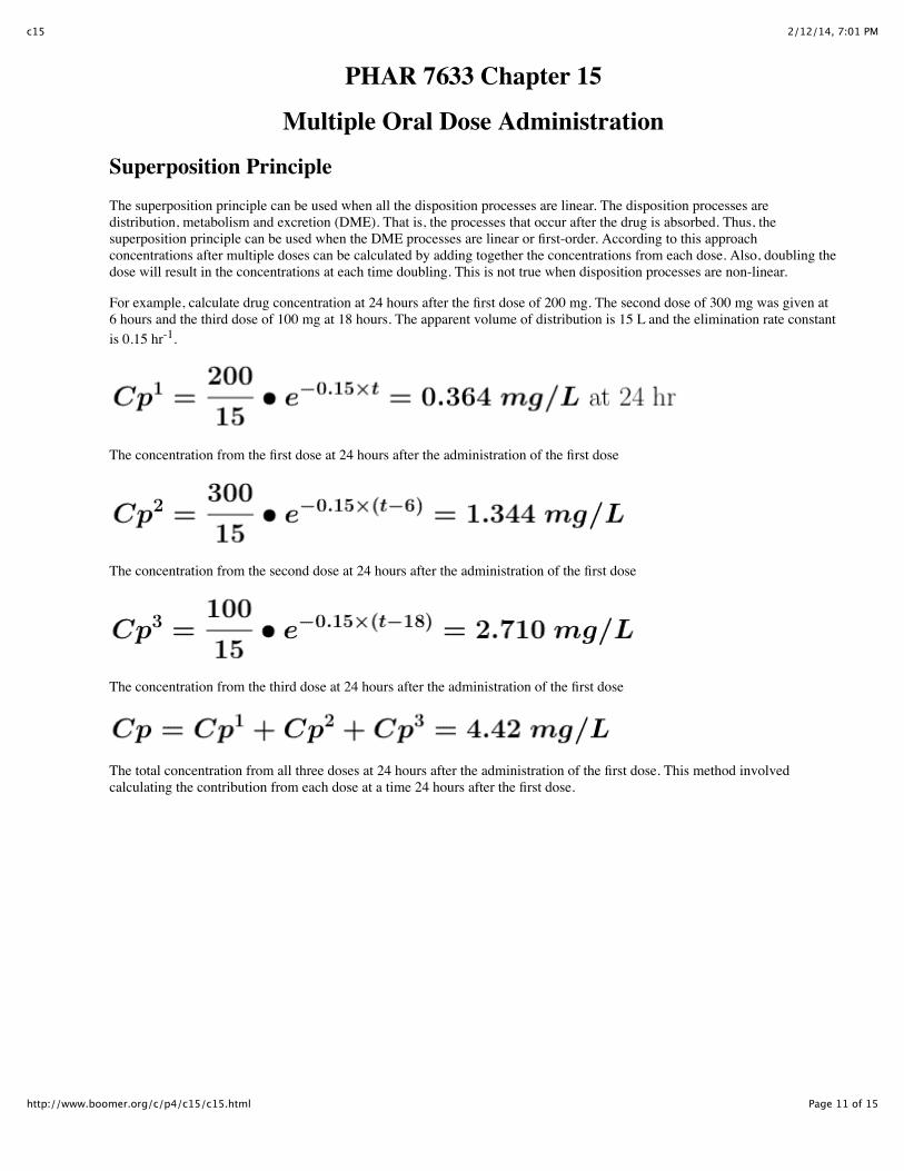
Superposition PrincipleThe superposition principle can be used when all the disposition processes are linear. The disposition processes aredistribution, metabolism and excretion (DME). That is, the processes that occur after the drug is absorbed. Thus, thesuperposition principle can be used when the DME processes are linear or first-order. According to this approachconcentrations after multiple doses can be calculated by adding together the concentrations from each dose. Also, doubling thedose will result in the concentrations at each time doubling. This is not true when disposition processes are non-linear.
For example, calculate drug concentration at 24 hours after the first dose of 200 mg. The second dose of 300 mg was given at6 hours and the third dose of 100 mg at 18 hours. The apparent volume of distribution is 15 L and the elimination rate constantis 0.15 hr-1.
The concentration from the first dose at 24 hours after the administration of the first dose
The concentration from the second dose at 24 hours after the administration of the first dose
The concentration from the third dose at 24 hours after the administration of the first dose
The total concentration from all three doses at 24 hours after the administration of the first dose. This method involvedcalculating the contribution from each dose at a time 24 hours after the first dose.
2/12/14, 7:01 PMc15
Page 12 of 15http://www.boomer.org/c/p4/c15/c15.html
The result of this calculation is shown graphically in Figure 15.5.1.
Figure 15.5.1 Drug Concentration after Three IV Bolus Doses
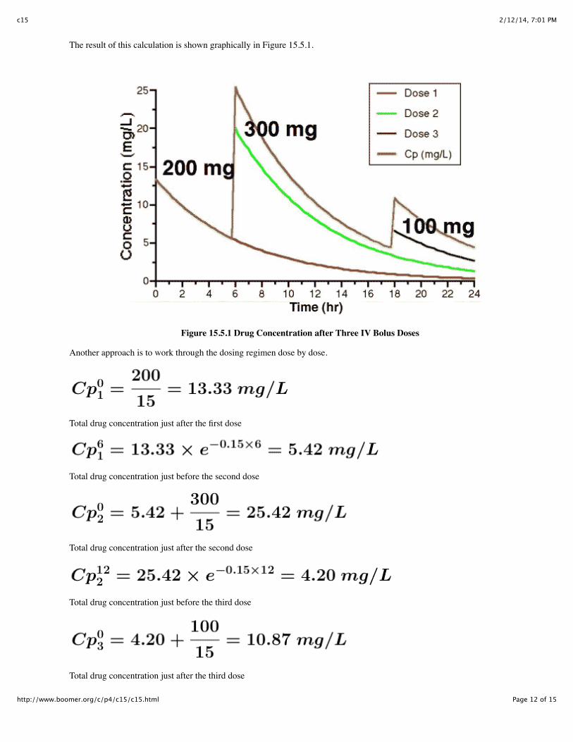
Another approach is to work through the dosing regimen dose by dose.
Total drug concentration just after the first dose
Total drug concentration just before the second dose
Total drug concentration just after the second dose
Total drug concentration just before the third dose
Total drug concentration just after the third dose

2/12/14, 7:01 PMc15
Page 13 of 15http://www.boomer.org/c/p4/c15/c15.html
Total drug concentration 6 hours after the third dose. This answer can also be calculated using an Excel spreadsheetillustrating the superposition principle.
Click on the figureto download and use this Excel spreadsheet
Figure 15.5.2 Excel™ Spreadsheet Illustrating the Superposition Principle - Multiple IV Doses
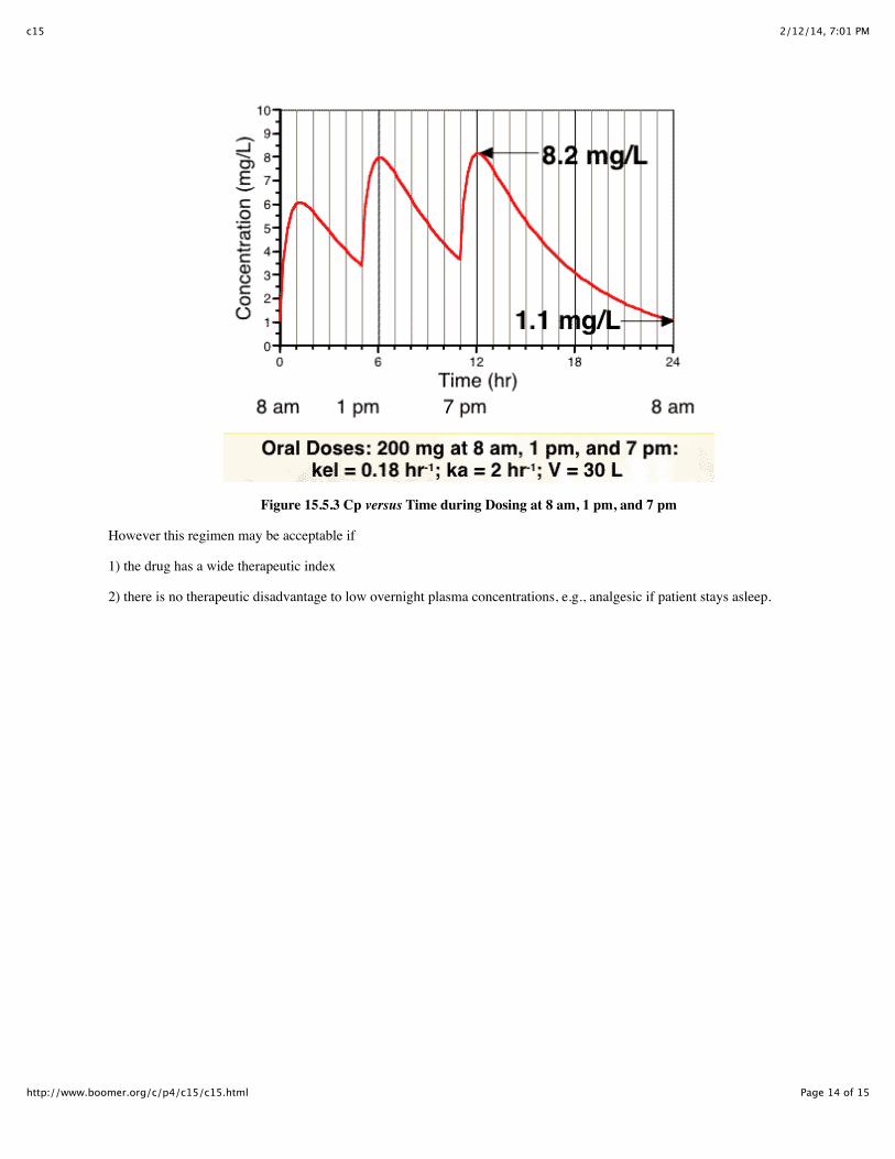
Non-uniform dosing intervalsPrior to this Chapter the calculations we have looked at consider that the dosing intervals are quite uniform, however,commonly this ideal situation is not adhered to completely.
Dosing three times a day may be interpreted as take with meals, the plasma concentration may then look like the plot in Figure60. The ratio between Cpmax and Cpmin is seven fold (8.2/1.1 = 7.45) in this example.
2/12/14, 7:01 PMc15
Page 14 of 15http://www.boomer.org/c/p4/c15/c15.html
Figure 15.5.3 Cp versus Time during Dosing at 8 am, 1 pm, and 7 pm
However this regimen may be acceptable if
1) the drug has a wide therapeutic index
2) there is no therapeutic disadvantage to low overnight plasma concentrations, e.g., analgesic if patient stays asleep.

2/12/14, 7:01 PMc15
Page 15 of 15http://www.boomer.org/c/p4/c15/c15.html
This regimen can be explored further using an Excel spreadsheet illustrating the superposition principle.
Click on the figureto download and use this Excel spreadsheet
Figure 15.5.4 Excel™ Spreadsheet Illustrating the Superposition Principle - Multiple Oral Doses AT Steady State
Other practice problems involving the calculation of Cp at three times during a uniform dosing interval with Linear or Semi-log graphical answers or calculation of Cp at three times during a non-uniform dosing interval with Linear or Semi-loggraphical answers
Student Objectives for this Chapter
This page (http://www.boomer.org/c/p4/c15/c1505.html) was last modified: Tuesday 05 Mar 2013 at 08:57 AM
Material on this website should be used for Educational or Self-Study Purposes Only
Copyright © 2001-2014 David W. A. Bourne ([email protected])