An Introduction to Formal Logic

Formal logic provides us with a powerful set of techniques for criticizing some arguments and showing others to be valid. Thesetechniques are relevant to all of us with an interest in being skilful and accurate reasoners. In this highly accessible book, Peter Smithpresents a guide to the fundamental aims and basic elements of formal logic. He introduces the reader to the languages of propositionaland predicate logic, and then develops formal systems for evaluating arguments translated into these languages, concentrating on theeasily comprehensible ‘tree’ method. His discussion is richly illustrated with worked examples and exercises. A distinctive feature is that,alongside the formal work, there is illuminating philosophical commentary. This book will make an ideal text for a first logic course, andwill provide a firm basis for further work in formal and philosophical logic.

PETER SMITH is Senior Lecturer in Philosophy at the University of Cambridge. His other books include Explaining Chaos (1998) andAn Introduction to Gödel’s Theorems (2007), and he is a former editor of the journal Analysis.

An Introduction toFormal Logic

Peter SmithUniversity of Cambridge

CAMBRIDGE UNIVERSITY PRESSCambridge, New York, Melbourne, Madrid, Cape Town, Singapore, São Paulo,Delhi, Mexico City

Cambridge University PressThe Edinburgh Building, Cambridge, CB2 8RU, UK

Published in the United States of America by Cambridge University Press, New York

www.cambridge.orgInformation on this title: www.cambridge.org/9780521801333

© Peter Smith 2003

This publication is in copyright. Subject to statutory exception and to the provisions of relevant collective licensing agreements, noreproduction of any part may take place without the written permission of Cambridge University Press.

First published 20036th printing 2013

Printed and bound in the United Kingdom by the MPG Books Group

A catalogue record for this publication is available from the British Library

ISBN 978-0-521-80133-3 HardbackISNB 978-0-521-00804-4 Paperback

Cambridge University Press has no responsibility for the persistence or accuracy of URLs for external or third-party internet websitesreferred to in this publication, and does not guarantee that any content on such we sites is, or will remain, accurate or appropriate.Information regarding prices, travel timetables and other factual information given in this work are correct at the time of first printing butCambridge University Press does not guarantee the accuracy of such information thereafter.

Contents Preface1 What is logic?2 Validity and soundness3 Patterns of inference4 The counterexample technique5 Proofs6 Validity and arguments

Interlude Logic, formal and informal

7 Three propositional connectives8 The syntax of PL9 The semantics of PL10 ‘A’s and ‘B’s, ‘P’s and ‘Q’s11 Truth functions12 Tautologies13 Tautological entailment

Interlude Propositional logic

14 PLC and the material conditional15 More on the material conditional16 Introducing PL trees17 Rules for PL trees18 PLC trees19 PL trees vindicated20 Trees and proofs

Interlude After propositional logic

21 Quantifiers22 QL introduced23 QL explored24 More QL translations25 Introducing QL trees26 The syntax of QL27 Q-valuations28 Q-validity29 More on QL trees30 QL trees vindicated

Interlude Developing predicate logic

31 Extensionality32 Identity33 The language QL=

34 Descriptions and existence35 Trees for identity36 Functions

Further readingIndex

Preface The world is not short of good introductions to logic. They differ widely in pace, style, the coverageof topics, and the ratio of formal work to philosophical commentary. My only excuse for writinganother text is that I didn’t find one that offered quite the mix that I wanted for my own students (first-year philosophy undergraduates doing a compulsory logic course). I hope that some other logicteachers and their students will find my particular combination of topics and approach useful.

This book starts from scratch, and initially goes quite slowly. There is little point in teachingstudents to be proficient at playing with formal systems if they still go badly astray when faced withground-level questions about the whole aim of the exercise. So I make no apology for working hard atthe outset to nail down some basic ideas.

The pace picks up as the book proceeds and readers get used to the idea of a formal logic. But eventhe more symbol-phobic students should be able to cope with most of the book, at least with a bit ofjudicious skipping. For enthusiasts, I give soundness and completeness proofs (for propositional treesin Chapter 19, and for quantifier trees in Chapter 30). The proofs can certainly be skipped: but I liketo think that, if explained in a reasonably relaxed and accessible way, even these more ‘advanced’results can in fact be grasped by bright beginners.

I have kept the text uncluttered by avoiding footnotes. You can follow up some of the occasionalallusions to the work of various logicians and philosophers (such as Frege or Russell) by looking atthe concluding notes on further reading.

The book has a web-site at www.logicbook.net. You will find there some supplementary teachingmaterials, and answers to the modest crop of exercises at the end of chapters. (And I’d like to hearabout errors in the book, again via the web-site, where corrections will be posted.)

I am very grateful to colleagues for feed-back, and to the generations of students who have more orless willingly road-tested versions of most of the following chapters. Special thanks are due to HilaryGaskin of Cambridge University Press, who first encouraged my plan to write this book, and theninsisted that I didn’t keep revising it for ever; to Dominic Gregory and Alexander Paseau, who readlate drafts of parts of the book, and provided many corrections; and to Laurence Goldstein, who didmuch more than it was reasonable to expect of a publisher’s reader.

Not least, I must thank Patsy and Zoë Wilson-Smith, without whose love and support this bookwould never have been finished.

Additional warm thanks are due to all those who kindly told me about mistakes in the first printedversion of the book. I have taken the opportunity of a reprint to make the needed corrections and tomake many other minor changes to improve clarity.

1

What is logic?

The business of logic is the systematic evaluation of arguments for internal cogency. And the kindof internal cogency that will especially concern us is deductive validity. But these brief headlinesleave everything to be explained.

What do we mean here by ‘argument’?What do we mean by evaluation for ‘internal cogency’?What do we mean, more particularly, by ‘deductive validity’?What sorts of ‘systematic’ evaluation of arguments are possible?

This introductory chapter makes a start on answering these questions.

1.1 What is an argument?By ‘argument’ we mean, roughly, a chain of reasoning in support of a certain conclusion. So we mustdistinguish arguments from mere disagreements and disputes. The children who shout at each other‘You did’, ‘I didn’t’, ‘Oh yes, you did’, ‘Oh no, I didn’t’, are certainly disagreeing: but they are notarguing in our sense, i.e. they are not yet giving any reasons in support of one claim or the other.

Reason-giving arguments are the very stuff of serious enquiry, whether it is philosophy or physics,literary criticism or experimental psychology. But of course, episodes of reasoning equally feature ineveryday, street-level, enquiry into what explains our team’s losing streak, the likely winner of nextmonth’s election, or the best place to train as a lawyer. For we quite generally want our opinions tobe true and to be defensible in the market-place of ideas, and that means that we should aim to havegood reasons backing up our opinions. That in turn means that we have an interest in being skilful andaccurate reasoners, using arguments which really do support their conclusions.

1.2 What sort of evaluation?The business of logic, then, is the evaluation of stretches of reasoning. Let’s take a very simple case(call it argument A).

Suppose you hold

(1) All philosophers are eccentric.

I then introduce you to Jack, who I tell you is a philosopher. So you come to believe

(2) Jack is a philosopher.

Putting these two thoughts together, you can obviously draw the conclusion

(3) Jack is eccentric.

This little bit of reasoning can now be evaluated along two quite independent dimensions.

First, we can ask whether the premisses (1) and (2) are true: are the ‘inputs’ to your reasoningcorrect? (1) in fact looks very disputable. And maybe Jack’s reflective skills are so limited thatwe’d want to dispute the truth of (2) as well.Second, we can ask about the quality of the inference from the premisses (1) and (2) to theconclusion (3). In this case, the movement of thought from the premisses (1) and (2) to theconclusion (3) is surely absolutely compelling. We have agreed that it may be open to questionwhether (1) and (2) are both true. However, if (1) and (2) are granted to be true (granted ‘for thesake of argument’, as we say), then (3) has got to be true too. There’s just no way that (1) and (2)could be true and yet (3) false. Someone who asserted that Jack is a philosopher, and that allphilosophers are eccentric, yet went on to deny that Jack is eccentric, would be implicitlycontradicting himself.

In brief, it is one thing to consider whether an argument starts from true premisses; it is another thingentirely to consider whether it moves on by reliable inferential steps. To be sure, we normally wantour arguments to pass muster on both counts. We normally want to start from true premisses and toreason by steps which will take us on to further truths. But it is important to emphasize that these aredistinct aims.

The premisses (and conclusions) of arguments can be about all sorts of topics: their truth is usuallyno business of the logician. If we are arguing about historical matters, then it is the historian who isthe expert about the truth of our premisses; if we are arguing about some matter of physics, then thephysicist is the one who can help us about the truth of our premisses; and so on. The specific concernof logic, by contrast, is not the truth of initial premisses but the way we argue from a given startingpoint. Logic is not about whether our premisses are true, i.e. match up to the world, but about whetherour inferences really do support our conclusions once the premisses are granted. It is in this sense thatlogic is concerned with the ‘internal cogency’ of our reasoning.

1.3 Deduction vs. inductionThe one-step argument A is a splendid bit of reasoning; if the premisses are true, then the conclusionis guaranteed to be true too. Here’s a similar case:

B (1) Either Jill is in the library or she is in the coffee bar.(2) Jill isn’t in the library.

So (3) Jill is in the coffee bar.

Who knows whether the premisses are true or not? But we can immediately see that necessarily, if thepremisses are true, then the conclusion will be true too: the inferential move is absolutely watertight.If premisses B(1) and B(2) here are both true, then B(3) cannot conceivably fail to be true.

Now consider the following contrasting case. Wild philosophical scepticism apart, you are

thoroughly confident that the cup of coffee you are drinking isn’t going to kill you (and if you weren’treally confident, you wouldn’t be calmly sipping as you read this, would you?). What justifies yourconfidence? Well, you believe something like

C (1) Cups of coffee that looked and tasted just fine haven’t killed you in the past.

You also know that

(2) This present cup of coffee looks and tastes just fine.

These premisses will prompt you to conclude

(3) This present cup of coffee won’t kill you.

And the inference that moves from the premisses C(1) and C(2) to the conclusion C(3) is, in thecircumstances, surely perfectly reasonable: the facts recorded in C(1) and C(2) do give you excellentgrounds for believing that C(3) is true. However – and here is the crucial contrast with the earlier‘Jack’ and ‘Jill’ examples – it isn’t the case that the truth of C(1) and C(2) absolutely guaranteesC(3) to be true too.

Perhaps someone has slipped a slow-acting tasteless poison into the coffee, just to make the logicalpoint that facts about how things have generally been in the past don’t guarantee that the trend willcontinue in the future.

Fortunately for you, C(3) no doubt is true. The tasteless poison is a fantasy. Still, it is a coherentfantasy. It illustrates the point that your grounds C(1) and C(2) for the conclusion that the coffee issafe to drink are strictly speaking quite compatible with the falsity of that conclusion. Someone whoagrees to C(1) and C(2) and yet goes on to deny C(3) might be saying something highly improbablegiven her premisses, but she won’t actually be contradicting herself. We can make sense of the idea ofC(1) and C(2) being true and yet C(3) false.

In his little book The Problems of Philosophy, Bertrand Russell has a nice example which presseshome the same basic point. Here is the chicken in the farmyard. Every day of its life, the farmer’swife has come into the hen yard in the morning to feed it. Here she comes again, bucket in hand. Thechicken believes that it is about to be fed, on the best possible evidence. But tough luck: today is theday when it gets its neck wrung. Again, what’s happened in the past is a very good guide to what willhappen next (what else can we rely on?): but reasoning from past to future isn’t absolutely watertight.

In summary, then, there is a crucial difference between the ‘Jack’ and ‘Jill’ examples on the onehand, and the ‘coffee’ example on the other. In the ‘Jack’ and ‘Jill’ cases, the premisses guarantee theconclusion. There is no conceivable way that A(1) and A(2) could be true and yet A(3) false:likewise if B(1) and B(2) are true then B(3) has to be true too. Not so with the ‘coffee’ case: it isconceivable that C(1) and C(2) are true while C(3) is false.

We’ll need some terminology to mark this difference: so, as a first shot definition, we will say

An inference step is deductively valid just if, given that its premisses are true, then itsconclusion is absolutely guaranteed to be true as well.

Equivalently, when an inference is deductively valid, we’ll say that the premisses logically entail theconclusion. So: arguments A and B each involve deductively valid inferential steps, but the coffeeargument C doesn’t. The latter argument instead involves reasoning from previously examined casesto a new case: this kind of extrapolation from the past to the future, or more generally from old casesto new cases, is standardly called inductive.

Note, the deductive/inductive distinction is not the distinction between good and bad reasoning.The ‘coffee’ argument is a perfectly decent one. It involves the sort of generally reliable reasoning towhich we rightly trust our lives, day in, day out. The conclusion is highly likely to be true given thepremisses. It is just that the inference in this case doesn’t guarantee that the conclusion is true, evenassuming the given premisses are true.

We’ll say very little more about inductive inferences in this book. They are an important anddifficult topic, but they are not our topic. Our concern is with arguments which aim to use deductivelyvalid inferences, where the premisses are supposed to logically entail the conclusion. And ourprincipal task will be to find various techniques for establishing whether a putatively valid inferentialmove really is deductively valid.

1.4 More examplesThe ‘Jack’ and ‘Jill’ arguments were examples where the inferential moves are obviously deductivelyvalid. Take the inference

D (1) All Republican voters support capital punishment.(2) Jo supports capital punishment.

So (3) Jo is a Republican voter.

That is equally obviously invalid. Even if D(1) and D(2) are true, D(3) doesn’t follow. Maybe lots ofpeople in addition to Republican voters support capital punishment, and Jo is one of them.

But questions of deductive validity needn’t be immediately obvious, one way or the other. Supposesomeone holds both of

E (1) Most Irish are Catholics.(2) Most Catholics oppose abortion.

On those grounds he concludes

So (3) At least some Irish oppose abortion.

What are we to make of this argument? I don’t know whether the premisses are true or not, andanyway that is hardly a matter for the logician (it is an empirical sociological matter to determine thedistribution of religious affiliation among the Irish, and to find out how many Catholics support theirchurch’s official teaching about abortion). So let’s leave aside the question of whether the premissesare in fact correct. What we can seek to determine here – from our armchairs, so to speak – iswhether the inferential move is valid: if the premisses are true, then must the conclusion be true too?

Suppose the Irish are a tiny minority of the world total of Catholics. Then it could be that nearly allthe other (non-Irish) Catholics oppose abortion, and hence most Catholics do, even though none of the

Irish oppose abortion. In other words, E(1) and E(2) could be true, yet E(3) false. The truth of thepremisses doesn’t absolutely guarantee the truth of the conclusion, so the inference step can’t be adeductively valid one.

Here’s a last example:

F (1) Some philosophy students admire all logicians.(2) No philosophy student admires any rotten lecturer.

So (3) No logician is a rotten lecturer.

Does this argument make a valid inferential move?So far, all we can do to find the answer is to cast around experimentally, trying to work out

somehow or other whether the truth of the premisses would guarantee the truth of the conclusion –though, as with the ‘Irish’ argument, a little thought should give the right answer (which is revealed in 3.1). Still, it would be good to be able to proceed more methodically and find some general

techniques for evaluating arguments like this. Ideally, we would like general techniques that workmechanically, that can be applied to settle questions of validity as automatically as we can settlearithmetical questions by calculation. But are such techniques for systematically evaluating argumentsever available?

Later we will explore some general techniques – though we will also have occasion to note thatthere are intriguing limitations on what can be done mechanically. First, however, we should say alittle more about what makes any kind of systematic approach possible.

1.5 The systematic evaluation of argumentsConsider again our first sample argument with its deductively valid inference step:

A (1) All philosophers are eccentric.(2) Jack is a philosopher.

So (3) Jack is eccentric.

And compare it with the following arguments:

A′ (1) All logicians are cool.(2) Russell is a logician.

So (3) Russell is cool.

A″ (1) All robins have red breasts.(2) Tweety is a robin.

So (3) Tweety has a red breast.

A″′ (1) All existentialists write bosh.(2) Sartre is an existentialist.

So (3) Sartre writes bosh.

(We can evidently keep on going ad nauseam, churning out arguments to the same A-pattern!)The four displayed arguments – and, of course, any others cast in the same mould – are all equally

good in the sense of all involving valid inference steps. In each case the truth of the premisses wouldlogically guarantee the truth of the conclusion. And plainly, it is no mere accident that the argumentsare all internally cogent. The validity of the inference move in the first argument hasn’t anythingespecially to do with being a philosopher or being eccentric. Likewise the validity of the inferencemove in the ‘robin’ argument isn’t due to special facts about robins. The four arguments all work forthe same reason: the shared pattern of inference is a reliable one.

We can describe the general principle here as follows.

Any inference step which moves from a pair of premisses, one of which says that everything of acertain kind has a given property, and the other of which says that a particular individual is ofthe former kind, to a conclusion which says that that individual has the latter property, isdeductively valid.

A moment’s reflection shows that this principle is a correct one. But we have hardly presented it inthe most perspicuous way. How much easier to put it instead like this:

Any inference step of the following type

All F are Gn is FSo, n is G

is deductively valid.

Here the italic letters ‘n’, ‘F’, ‘G’ are used to exhibit the skeletal pattern of an argument (with ‘n’holding the place for a name, ‘F’ and ‘G’ for predicates, i.e. expressions which attribute properties orpick out kinds of thing). How we flesh out the skeletal pattern or schema doesn’t matter: any sensibleway of substituting for the schematic variables (as we’ll call the likes of ‘n’, ‘F’, ‘G’) will yieldanother argument with a valid inference step of the same type.

We said at the outset, logic is concerned with the systematic study of validity. We now get a firstglimpse of how systematicity might be achieved – by noting that the same patterns or forms ofinference can appear in many different partic- ular arguments.

Some inference patterns like the one just shown are reliable. Others aren’t. For example, considerthis pattern of inference:

Most F are GMost G are HSo, at least some F are H

This is the pattern of inference the ‘Irish’ argument was relying on, and we saw that it doesn’t work.There will be much more on the idea of patterns of inference in later chapters; but first, a quick

summary.

1.6 SummaryWe can evaluate a piece of reasoning in two distinct ways. We can ask whether the premisses

are actually true. And we can ask whether the truth of the premisses actually supports the truth ofthe conclusion. Logic is concerned with the second dimension of evaluation: i.e. the province oflogic is the question whether a given argument internally hangs together, whether its inferentialmoves are cogent ones.We are setting aside inductive arguments (and other kinds of non-conclu-sive reasoning). Wewill be concentrating on arguments involving inferences that purport to be deductively valid. Inother words, we are going to be concerned with the study of inferences that aim to logicallyentail their conclusions – aim to be, as it were, absolutely watertight. (Imagine an argument as ahydraulic device: if truth is poured in at the top, then we want it to trickle down to the bottom.The arguments with non-conclusive, possibly leaky, inference moves are ones where puttingtruth in at the top doesn’t guarantee getting any truth out at the bottom; the deductively validinferences are those where truth in guarantees truth out.)Arguments typically come in families whose members share good or bad types of inferentialmove; looking at such general patterns of inference will be a step towards making logic asystematic study.

Exercises 1By ‘conclusion’ we do not simply mean what concludes, what is stated at the end of, a passage ofreasoning. We mean what the reasoning aims to establish – and that might in fact be stated at the outsetof an argument. Likewise, ‘premiss’ does not mean (contrary to what the Concise Oxford Dictionarysays!) ‘a previous statement from which another is inferred’. Reasons supporting a certain claimmight well be given after the target conclusion has been stated.

Indicate the premisses and conclusions of the following arguments. Which of these arguments doyou suppose involve deductively valid reasoning? Why? (We haven’t developed any techniques foryou to use yet: just improvise and answer the best you can!)

1. Whoever works hard at logic does well. Accordingly, if Russell works hard at logic, hedoes well.

2. Most politicians are corrupt. After all, most ordinary people are corrupt – and politiciansare ordinary people.

3. It will snow tonight. For the snow clouds show up clearly on the weather satellite,heading this way.

4. Anyone who is well prepared for the exam, even if she doesn’t get an A grade, will atleast get a B. Jane is well prepared, so she will get at least a B grade.

5. John is taller than Mary; and Jane is shorter than Mary. So John is taller than Jane.6. At eleven, Fred is always either in the library or in the coffee bar. And assuming he’s in

the coffee bar, he’s drinking an espresso. Fred was not in the library when I looked ateleven. So he was drinking an espresso then.

7. The Democrats will win the election. For the polls put them 20 points ahead, and no partyhas ever overturned even a lead of 10 points with only a week to go to polling day.

8. Jekyll isn’t the same person as Hyde. The reason is that no murderers are sane – but Hydeis a murderer, and Jekyll is certainly sane.

9. No experienced person is incompetent. Jenkins is always blundering. No competentperson is always blundering. Therefore Jenkins is inexperienced.

10. Many politicians take bribes. Most politicians have extra-marital affairs. So many peoplewho take bribes have extra-marital affairs.

11. (Lewis Carroll) Babies cannot manage crocodiles. Because babies are illogical. Butillogical persons are despised. And nobody is despised who can manage a crocodile.

12. (Lewis Carroll again) No interesting poems are unpopular among people of real taste. Nomodern poetry is free from affectation. All your poems are on the subject of soap bubbles.No affected poetry is popular among people of real taste. Only a modern poem would beon the subject of soap bubbles. Therefore all your poems are uninteresting.

13. ‘If we found by chance a watch or other piece of intricate mechanism we should infer thatit had been made by someone. But all around us we do find intricate pieces of naturalmechanism, and the processes of the universe are seen to move together in complexrelations; we should therefore infer that these too have a maker.’

14. ‘I can doubt that the physical world exists. I can even doubt whether my body reallyexists. I cannot doubt that I myself exist. So I am not my body.’

2

Validity and soundness

The first chapter briefly introduced the idea of an inferential move being deductively valid. Thischapter explores the idea of validity in a little more depth, and also emphasizes the centrality ofdeductive reasoning.

2.1 Validity and possibilityWe said that an inference step is valid just if, given the input premisses are true, then the outputconclusion is absolutely guaranteed to be true as well. But what do we mean here by an ‘absoluteguarantee’?

Previously, we gave a number of other, equally informal, explanations of the idea of validity interms of what is ‘conceivable’ or what it would be ‘self-contra-dictory’ to assert. Here now isanother definition of validity: and this time, it is a version of the standard, ‘classical’, textbookdefinition of validity.

An inference step from given premisses to a particular conclusion is (classically) valid if andonly if there is no possible situation in which the premisses would be true and the conclusionfalse.

We’ll take this as our official definition from now on. But it is only as clear as the notion of a‘possible situation’. It needs to be stressed, then, that ‘possible’ here is meant in the widest sense – asense related to those ideas of what is ‘conceiv-able’, or ‘involves no contradiction’ that we metbefore.

Consider, for example, this inference:

Premiss: Jo jumped out of a twentieth floor window (without parachute, safety net, etc.) andfell freely and unimpeded onto a concrete pavement.

Conclusion: Jo was injured.

And let’s grant that there is no situation that can really obtain in the actual world, with the laws ofphysics as they are, in which the premiss would be true and the conclusion false. In the world as it is,falling unimpeded onto concrete from twenty floors up will always produce serious (surely fatal)injury. Does that make the inference from the given premiss to the conclusion deductively valid?

No. Although it isn’t, let’s agree, physically possible to jump in those circumstances without beinginjured, it remains possible in a weaker sense: it is ‘logically possible’, if you like. We cancoherently conceive of situations in which the laws of nature are different or are miraculously

suspended, and someone jumping from twenty floors up will float delicately down like a feather.There is no internal logical contradiction in that idea. And all that is required for the deductiveinvalidity of an inference is that it is possible in this very weak sense for the premisses to be trueand the conclusion false. As we put it before, an inference is invalid if there is no internalcontradiction in the notion of the truth of the premisses being combined with the falsity of theconclusion.

This very weak notion of logical possibility (any consistent fantasy counts as possible in thissense) goes with a correspondingly strong notion of logical impossibility. If something is logicallyimpossible, like being circular and square at the same time, then it is absolutely ruled out: the veryidea is inconsistent, incoherent, logically absurd. For a classically valid inference, it is impossible inthis very strong sense for the premisses to be true and the conclusion false.

It will be useful to introduce a further definition:

A set of propositions is logically consistent if it is logically possible for the propositions all tobe true together. Likewise, a set of propositions is logically inconsistent if it is logicallyimpossible for the propositions to be true together.

If there is no possible situation in which a bunch of premisses would be true and a certain conclusionfalse, then the premisses and the denial of the conclusion form an inconsistent set of propositions. Soanother way of characterizing the notion of validity is this: an inference is classically valid if thepremisses taken together with the denial of the conclusion form an inconsistent set.

To be sure, we have still only gestured at the notions of logical possibility and logicalimpossibility that are in play here. As we go along, we will need to sharpen up our understanding ofthese ideas. Still, we’ve said enough to get us started.

2.2 What’s the use of deduction?It needs to be stressed again that deductively valid inferences are not the only acceptable ones.Inferring that Jo is injured from the fact she fell twenty stories onto concrete is perfectly reasonable.Inductive reasoning like this is very often good enough to trust your life to: the premisses may renderthe conclusion a racing certainty. But such reasoning isn’t deductively valid.

Now consider a more complex kind of inference: take the situation of the detective – call himSherlock. In the ideally satisfying detective story, Sherlock assembles a series of clues and thensolves the crime by an inference to the best explanation. In other words, the detective arrives at anhypothesis that neatly accommodates all the strange events and bizarre happenings, an hypothesis thatstrikes us (once revealed) as obviously the right explanation. Why is the bed bolted to the floor? Whyis there a useless bell rope hanging by the bed? Why is there a ventilator near the top of the ropeleading through into the next room? What is that strange music heard at the dead of night? All thepieces fall into place when Sherlock infers a dastardly plot to kill the sleeping heiress in herunmovable bed by means of a poisonous snake, trained to descend the rope in response to the music.But although this is an impressive ‘deduction’ in one everyday sense of the term, it is not deductivelyvalid reasoning in the logician’s sense. We may have a set of clues, and some hypothesis H may be theonly plausible explanation we can find: but in the typical case it won’t be a contradiction to supposethat, despite the way the evidence stacks up, our hypothesis H is false. That won’t be a logically

inconsistent supposition, only a very unlikely one. Hence, the detective’s plausible ‘deductions’ arenot (normally) valid deductions in the logician’s sense.

This being so, we might begin to wonder: if our inductive reasoning about the future on the basis ofthe past is not deductive, and if inference to the best explanation is not deductive either, just howinteresting is the idea of deductively valid reasoning?

To make the question even more worrisome, consider that paradigm of systematic rationality,scientific reasoning. We gather data, and try to find the best theory that fits; rather like the detective,we aim to come up with the best explanation of the actually observed data. But a useful theory goeswell beyond merely summarizing the data. In fact, it is precisely because the theory goes beyond whatis strictly given in the data that the theory is useful for making novel predictions. Yet since the excesscontent isn’t guaranteed by the data, because it is (in a broad sense) an induction beyond the data, thetheory cannot be validly deduced from observation statements. So again it might be asked: what’s theinterest of deductive validity, except maybe to mathematicians, if deductive inference doesn’t featureeven in the construction of scientific theories?

But that’s too quick! It is true that we can’t simply deduce a theory from the data it is based on.However, it just doesn’t follow that deductive reasoning plays no essential part in scientificreasoning.

Here’s a picture of what goes on in science. Inspired by patterns in the data, or by models of theunderlying processes, or by analogies with other phenomena, etc., we conjecture that a certain theoryis true. Then we use the conjectured theory (together with assumptions about ‘initial conditions’) todeduce a range of testable predictions. The first stage, the conjectural stage, may involve flair andimagination, rather than brute logic, as we form our hypotheses about the underlying processes. But atthe second stage, having made our conjectures, we need to infer testable consequences; and this doesinvolve deductive logic. For we need to examine what else must be true if the theory is true: we wantto know what our hypothesized theory logically entails. Once we have deduced testable predictions,we seek to check them out. Often our predictions turn out to be false. We have to reject the theory. Orelse we have to revise it as best we can to accommodate the new data, and then go on to deduce moretestable consequences. The process is typically one of repeatedly improving and revising ourhypotheses, deducing consequences which we can test, and then refining the hypotheses again in thelight of test results.

This hypothetico-deductive model of science (which highlights the role of deductive reasoningfrom theory to predictions) no doubt itself needs a lot of development and amplification andrefinement. But with science thus conceived, we can see why deduction is absolutely central to theenterprise after all.

2.3 The invalidity principleClassical validity is defined in terms of possibility and necessity. An inference is valid if it isimpossible for the premisses to be true and the conclusion false. Valid inferences are necessarilytruth-preserving. So, to evaluate for validity, we usually have to consider not only what is the case inthe actual world but also consider alternative ways things might have been – or, to use a helpfulimage, we need to consider what is the case ‘in other possible worlds’. Take, for example, thefollowing argument:

A (1) No Welshman is a great poet.

(2) Shakespeare is a Welshman.So (3) Shakespeare is not a great poet.

The premisses and conclusion are all false. But this fact is quite compatible with the inferential movehere being a valid one. Which indeed it is. For there is no possible situation in which the premisseswould be true and the conclusion false. In other words, any possible world which did make thepremisses true (Shake-speare being brought up some miles to the west, and the Welsh not going in forverse), would also make the conclusion true.

Take a couple more examples:

B (1) No father is female.(2) Bill Clinton is a father

So (3) Bill Clinton is not female.

C (1) No one whose middle name is ‘Winifrid’ is a Democrat.(2) George W. Bush’s middle name is ‘Winifrid’.

So (3) George W. Bush is not a Democrat.

These again are valid inferences (cut to the same reliable pattern as the Shakespeare inference), butthe inference step leads in argument B from true premisses to a true conclusion, and in argument Cfrom false premisses to a true conclusion.

That last claim may for a moment seem odd: how can a truth be validly inferred from twofalsehoods? Well, C(3) is true – George W. Bush is a Republican – but here in the actual world it hasnothing to do with facts about his middle name. It just happens to be true quite independently, andsomeone who believed C(3) on the basis of the daft premisses C(1) and C(2) would be right merelyby luck. Still, the point remains that in any world where those premisses were true, C(3) would alsobe true, and so the inference step is deductively valid.

There can of course be mixed cases too, with some true and some false premisses. So allowing forthese, we have in summary:

A valid inference can have actually true premisses and a true conclusion, (some or all) actuallyfalse premisses and a false conclusion, or (some or all) false premisses and a true conclusion.The only combination ruled out by the definition of validity is having all true premisses and afalse conclusion. Validity is about the necessary preservation of truth – so a valid inferencecannot take us from actually true premisses to a false conclusion.

That last point is worth stressing, and indeed we might usefully dignify it with a label:

The invalidity principle An inference with actually true premisses and an actually falseconclusion can’t be deductively valid.

We’ll see in 4.1 how this invalidity principle gets to do interesting work when combined with theobservation that arguments come in families sharing the same kind of inference step. But here’s an

immediate (if rather trivial) application. Consider the following line of reasoning:

D (1) No England cricket captain has written a world-famous philosophy text book.

(2) All world-famous philosophy text books are written by people with some knowledgeof philosophy.

(3) Anyone who has taught philosophy at a university has some knowledge of philosophy.So (4) No one who has taught philosophy at a university has captained England at cricket.

Here we have a three-premiss inference with a certain complexity, and it may take a moment’s thoughtto figure out whether the inferential move is valid or not.

The question is immediately settled, however, once you put together the fact that the premisses areall true with the esoteric bit of information that the conclusion is actually false (as it happens, theone-time England captain Mike Brear-ley previously was a university lecturer in philosophy). Hence,by the invalidity principle, the inference move in D must be invalid: and that settles that!

2.4 Inferences and argumentsSo far, we have spoken of inferential steps in arguments as being valid or invalid. For the moment,we’ll largely stick to this way of talking. But it is more common simply to describe arguments asbeing valid or otherwise. In that usage, we say that a one-step argument, like those we’ve beenlooking at so far, is valid just if the inference step from the premiss(es) to the conclusion is valid.

This is absolutely standard shorthand. But it can mislead beginners. After all, saying that anargument is ‘valid’ can sound rather like an all-in endorsement. However, to repeat, to say that anargument is valid is only to commend the cogency of the inferential move between premisses andconclusion. A valid argument, i.e. one that is internally cogent like A, can still have premisses that arequite hopelessly false.

It is useful, then, to have a term for arguments that do deserve all-in endorsement – which both startfrom truths and proceed by deductively cogent inference steps. The usual term is ‘sound’. So:

A (one-step) argument is valid just if the inference from the premisses to the conclusion is valid.

A (one-step) argument is sound just if it has all true premisses and the inference from thosepremisses to the conclusion is valid.

A few authors annoyingly use ‘sound’ to mean what we mean by ‘valid’. But everyone agrees there isa key distinction to be made between mere deductive cogency and the all-in virtue of having truepremisses and making a cogent inference. There’s just an irritating divergence over how this agreeddistinction should be labelled. Our usage of the labels is the majority one.

We typically want arguments that aim at deductive success to be sound in our double-barrelledsense. But not always! Sometimes we argue from premisses we think are false (or even inconsistent)precisely to bring out some absurd consequence of them, in the hope that a disputant will agree thatthe consequence is absurd and so come to accept that the premisses aren’t all true.

Note three immediate consequences of our definition:

(a) any sound argument has a true conclusion;(b) no pair of sound arguments can have inconsistent conclusions;(c) no sound argument has inconsistent premisses.

First, a sound argument starts from actually true premisses and involves a necessarily truth-preservinginference move – so it must end up with an actually true conclusion. Second, since a pair of soundarguments will have a pair of actually true conclusions, that means that the conclusions are truetogether. If they are actually true together, then of course they can be true together. And if they can betrue together then (by definition) the conclusions are consistent with each other. Finally, since a bunchof inconsistent premisses cannot all be true together, an argument starting from those premisses cannotfulfil the first half of the definition of soundness.

Replacing ‘sound’ by ‘(classically) valid’ in (a) to (c) yields falsehoods, however. That is easy tosee in the first two cases. For the third case, reflect again that sometimes we show that certainpremisses are implicitly inconsistent by validly drawing some explicit contradiction from them: we’llreturn to explore this point in Chapter 5.

2.5 What sort of thing are premisses and conclusions?The basic constituents of arguments are premisses and conclusions. But what sort of thing are they?Well, for a start, they are the sort of thing that can be true or false; and we’ll follow one convention bycalling the bearers of truth or falsity, whatever they should turn out to be, propositions. So in ourusage, arguments are uncontentiously made up out of propositions: but what are they?

A terminological aside Propositions, such as premisses and conclusions, are assessed fortruth/falsity. Inference moves are assessed for validity/ invalidity. These dimensions ofassessment, as stressed before, are fundamentally different: so we should mark the distinctionvery carefully. Despite the common misuse of the terms, we should never say that a propositionis ‘valid’ when we mean it is true, or that an argument is ‘true’ when we mean that it is valid (orsound).

You might suggest: propositions are just declarative sentences (like ‘Jack kicks the ball’ asopposed to questions like ‘Does Jack kick the ball?’, or imperatives like ‘Jack, kick the ball!’). But itwould be odd to identify premisses and conclusions with sentences in the sense of the actual printedinscriptions, particular physical arrays of blobs of ink on the page. Surely we want to say that thesame premisses and conclusions can appear in the many different printed copies of this book (orindeed, when the book is read aloud). So the suggestion is presumably that propositions aredeclarative sentence types, which can have printed instances appearing in many copies (and can havemany spoken instances too).

But even so understood, the suggestion is not without difficulties. Consider (a) an ambiguoussentence like the proverbial wartime headline ‘Eighth Army push bottles up Germans’ – are theGermans being bottled up by a push, or are the Eighth Army pushing bottles? The sentence says twodifferent things, one of which may be true and the other false: so, same sentence, different things said,i.e. different propositions expressed. What about (b) sentences involving pronouns? For example,consider the argument ‘No logician is irrational. Russell is a logician. So, he is rational.’ Wenaturally read this as a valid argument. But the conclusion as written is in a sense incompletely

expressed. Who is being referred to by ‘he’? In context, we take it to be Russell. In another context,the pronoun ‘he’ could refer to someone else. And ripped out of all context, an occurrence of ‘He isrational’ wouldn’t convey any determinate message – wouldn’t express any particular proposition. Soagain, same sentence but expressing different propositions (or none). (c) There can be conversecases, where it seems natural to say that different sentences express the same proposition. After all,don’t ‘Snow is white’ and ‘La neige est blanche’ say the same? Or within a language, how about ‘Jackloves Jill’ and ‘Jill is loved by Jack’?

Some find these sorts of reasons for distinguishing sentences and propositions compelling, andconclude that propositions aren’t sentences but are – as we’ve just been saying – what are expressedby declarative sentences. Others respond that cases of ambiguity and incompleteness only show thatwe need to identify propositions with fully interpreted sentences (i.e. sentences parsed as having acertain meaning, and with the reference of pronouns such as ‘he’, etc. deter-mined); and they will saythat cases of equivalent sentences (whether from different languages or the same one) are no morethan that – i.e. we have equivalent but still distinct propositions.

We aren’t going to try to settle that dispute. That may sound rather irresponsible. But it will turn outthat for our purposes later in this book, we don’t actually need to settle the nature of propositionshere. So we fortunately can leave that tricky issue in ‘philosophical logic’ hanging as we proceedwith our more formal explorations.

2.6 SummaryAlthough inductive arguments from past to future, and inferences to the best explanation, are notdeductive, the hypothetico-deductive picture shows how there can still be a central role fordeductive inference in scientific and other enquiry.An inference step is (classically) valid if and only if there is no possible situation in which itspremisses are true and the conclusion false.The relevant notion of a possible situation is (roughly) the notion of a coherently conceivablesituation, one whose characterization involves no internal contradiction.A one-step argument is valid if and only if its inference step is valid.An argument which is valid and has true premisses is said to be sound.The constituents of arguments (premisses and conclusions) are propositions. But we needn’tsettle the nature of propositions.

Exercises 2Which of the following claims are true, which false, and why?

1. If someone produces an invalid argument, his premisses and conclusion must make alogically inconsistent set.

2. If an argument has false premisses and a true conclusion, then the truth of the conclusioncan’t really be owed to the premisses: so the argument cannot really be valid.

3. Any inference with actually true premisses and a true conclusion must be truth-preservingand so valid.

4. If the conclusion of an argument is false and all its premisses are true, then the argumentcannot be deductively valid.

5. You can make a valid inference invalid by adding extra premisses.

6. You can make a sound inference unsound by adding extra premisses.7. You can make an invalid inference valid by adding extra premisses.8. If a set of propositions is consistent, then adding a further true proposition to it can’t make

it inconsistent.9. If a set of true propositions is consistent, then adding a further false proposition to it must

make it inconsistent.10. If a set of propositions is inconsistent, then if we remove some proposition P, we can

validly infer that P is false from the remaining propositions in the set.

3

Patterns of inference

We noted in the first chapter how arguments can come in families which share the same pattern ofinference step. We now explore this idea in more detail.

3.1 More patternsConsider again the argument:

A (1) No Welshman is a great poet.(2) Shakespeare is a Welshman.

So (3) Shakespeare is not a great poet.

The inference step here is deductively valid. Likewise for the parallel ‘Clinton’ and ‘Bush’ argumentsin 2.3. These are valid too:

A′ (1) No three-year old understands quantum mechanics.(2) Daisy is three years old.

So (3) Daisy does not understand quantum mechanics.

A″ (1) No elephant ever forgets.(2) Jumbo is an elephant.

So (3) Jumbo never forgets.

And we can improvise endless variations on the same theme.The inference steps in these arguments aren’t validated by any special facts about poets, presidents,

three-year-olds or elephants. Rather, they are all valid for the same reason, namely the meaning of‘no’ and ‘not’ and the way that these logical concepts distribute in the premisses and conclusion. Infact, we have

Any inference of the type

No F is Gn is FSo, n is not G

is valid.

As before ( 1.5), ‘F’ and ‘G’ here stand in for predicates – expressions that attribute properties like

being an elephant or understanding quantum mechanics – and ‘n’ holds the place for a name. Noteagain that this sort of use of symbols is in principle dispensable. We could say, e.g.,

Any one-step inference is valid which has one premiss which says that nothing of some givenkind has a certain property, whose other premiss says that a certain individual is of the givenkind, and whose conclusion says that the individual in question lacks the property in question.

But it is surely a lot more transparent to use the symbolic shorthand.Let’s be clear, then, that there is nothing essentially mathematical involved in this use of symbols

like ‘F’ and ‘n’. We are simply exploiting the fact that it is easier to talk about a pattern of inferenceby displaying the pattern using these ‘schematic variables’, instead of trying to describe it incumbersome words.

Here’s another, slightly trickier, example which we have met before ( 1.4):

B (1) Some philosophy students admire all logicians.(2) No philosophy student admires any rotten lecturer.

So (3) No logician is a rotten lecturer.

Do the premisses logically entail the conclusion?Suppose the premisses are true. Then by B(1) there are some philosophy students (as it might be,

Jack and Jill) who admire all logicians. We know from B(2) that Jack and Jill (since they arephilosophers) don’t admire rotten lecturers. That is to say, people admired by Jack and Jill aren’trotten lecturers. So in particular B(3), logicians – who are all admired by Jack and Jill – aren’t rottenlecturers. The inference is valid.

Having now done the work for the argument about rotten lecturers, and shown that it is valid, whatabout this following argument?

B′ (1) Some opera fans buy tickets for every new prod uction of Wagner’s Siegfried.(2) No opera fan buys tickets for any merely frivolous entertainment.

So (3) No new production of Wagner’s Siegfried is a merely frivolousentertainment.

That again is valid; and a moment’s reflection shows that it essentially involves the same type ofinference move as before, and can be shown to be valid in just the same kind of way. We could put itsymbolically like this:

Any inference of the type

Some F have relation R to every GNo F has relation R to any HSo, no G is H

is valid.

By talk of a relation we just mean whatever is expressed by a predicate with (as it were) more thanone slot in it waiting to be filled by subject terms. For example the predicate ‘… loves …’ has two

empty places waiting to be filled up by names like ‘Romeo’ and ‘Juliet’ (or by more complex termslike ‘Someone in this room’ and ‘every philosopher’). Likewise, ‘… is married to …’ also expressesa two-place relation, as does ‘… is taller than …’ and (to return to our examples) ‘… admires …’and ‘… buys tickets for …’. So, with that notion of a relation in play, we can see that the arguments Band B′ do share the same indicated pattern of inference.

And just try expressing that common pattern without using the symbols: it can be done, to be sure,but at what cost in perspicuity!

In summary, then, we have now displayed three examples of general patterns of valid inference. In 1.5 we noted the simple inference pattern

All F are Gn is FSo, n is G

We have just noted the pattern

No F is Gn is FSo, n is not G

and, rather more complicatedly,

Some F have relation R to every GNo F have relation R to any HSo, no G is H

Any inference following one of these three patterns will be valid. To repeat, it is not the specialsubject matter of the instances that makes them valid. The way that ‘all’, ‘every’ and ‘any’, ‘some’,‘no’ and ‘not’ distribute between the premisses and conclusion suffices for validity in these cases.

Here are some more examples of reliable inference patterns (with varying numbers of premisses –there is nothing special about having exactly two):

No F is GSo, no G is FAll F are HNo G is HSo, no F is GAll F are either G or HAll G are KAll H are KSo, all F are K

(Construct some instances, and convince yourself that your examples and other inferences of the sametypes will all be valid.)

In sum, evaluating a particular argument for validity very often goes with seeing a certain generalpattern of inference as doing the work in the argument. And evaluating this inference pattern will, inone fell swoop, simultaneously give a verdict on a whole range of arguments making the same sort ofinferential move. This point underlies the whole business of logic as a systematic study – though, as

we will explain in 3.4 below, the point does need to be handled with a bit of care. But first …

3.2 Three simple points about inference patternsPoint One Take again the inference pattern

All F are Gn is FSo, n is G

Does the following inference count as an instance of the pattern?

C (1) All men are mortal.(2) Snoopy is a dog.

So (3) Bill Clinton is female.

Of course not! True, when taken separately, C(1) is of the form All Fs are G (i.e. attributes a certainproperty to everything in some class), C(2) is a simple sub-ject/predicate claim of the form n is F,and likewise C(3) has the form n is G. But when we describe an inference as having a pair ofpremisses of the pattern

All F are Gn is F

and a conclusion

n is Gwe are indicating that the same predicate F is involved in the two premisses. Likewise, the name nand predicate G that are in the premisses should recur in the conclusion. The whole point of theschematic variables is to represent patterns of recurrence in the premisses and conclusion. So inmoving back from an abstract schema to a particular instance of the type, we must preserve thepatterns of recurrence by being consistent in how we interpret the ‘F’s and ‘G’s and ‘n’s. A schematicvariable is to be filled out the same way at each occurrence in the schema.

What about the following argument? Does this count as an instance of the displayed inferencepattern?

D (1) All philosophers are philosophers.(2) Socrates is a philosopher.

So (3) Socrates is a philosopher.

This time, instead of substituting at random, we have at least been consistent – though we havesubstituted in the same way for both ‘F’ and ‘G’. We will allow this as a special case. The crucialthing, to repeat, is that we must hold the interpretation of each of ‘F’ and ‘G’ fixed throughout theargument. If an argument pattern is reliably valid whatever the substitutions for ‘F’ and ‘G’, etc., itwill still be valid in the trivializing case where what is substituted for the ‘F’s and ‘G’s happens to

be the same.And indeed argument D is classically valid by our definition: it can’t have true premisses and a

false conclusion. The inference is certainly no use at all as a means for persuading someone of theconclusion who does not already accept that very proposition! But there’s an important distinction tomake here: truth-preservation is one thing, persuasiveness is something else. And once we firmlymake that distinction, counting D as deductively virtuous is acceptable. After all, an inference thatcovers no ground hasn’t got a chance to go wrong! (We will return to expand this remark in Chapter6.)

Point Two Consider the two arguments:

E (1) All men are mortal.(2) Socrates is a man.

So (3) Socrates is mortal.

E′ (1) Socrates is a man.(2) All men are mortal.

So (3) Socrates is mortal.

What’s the relation between the inferences here? Validity, recall, is defined this way: an inference isvalid just when there is no possible situation in which all the premisses are true and the conclusionfalse. Assessments of validity for inference steps are therefore quite blind to the order in which thepremisses are ‘fed in’. Hence for our purposes – concentrating, as logic does, on assessments ofvalidity – the order in which the premisses of an inference step are presented is irrelevant. So we’lltake the two E arguments as involving the same inference step. And generalizing, we’ll take twoschemas

All F are Gn is FSo, n is Gn is FAll F are GSo, n is G

as representing the same basic pattern of inference.

Point Three What is the relation between that pattern and these ones? –

All H are Km is HSo, m is KAll Φ are Ψα is ΦSo, α is Ψ

All are is

So, is

Again, all four schemas are just more possible ways of representing the same kind of inferentialmove. The choice of ‘F’s and ‘G’s as against ‘H’s and ‘K’s, or Greek letters, or some other place-holders, doesn’t matter at all; what we are trying to reveal is a pattern of recurrence, and the ‘F’s or‘Φ’s or whatever are just used to mark different places in the pattern. (It would be a rather badmistake, then, to identify the pattern of inference with one or other of these various symbolicexpressions used to display the pattern.)

3.3 Generality and topic neutralityOur examples so far have all had a very abstract structure. But consider:

F (1) Jill is a mother.So (2) Jill is female.

G (1) Jack has a first cousin.So (2) Jack’s parents are not both only children.

H (1) Tom is taller than Dick.(2) Dick is taller than Harry.

So (3) Tom is taller than Harry.

These arguments are all valid. If Jill is a mother, she is a female parent, and hence female. If Jack hasa first cousin (where a first cousin, by definition, is a child of one of his aunts or uncles) he must havean aunt or uncle. So his parents cannot both have been only children. And if three people are lined upin descending order of height, then the first must be taller than the last.

Now, in each case we can expose some inferentially relevant structure. The first two arguments arenot made valid by something peculiar to Jill or Jack. Any inference of these kinds is valid:

n is a motherSo, n is femalen has a first cousinSo, n’s parents are not both only children

Likewise, any argument with the following pattern is valid:

k is taller than ll is taller than mSo, k is taller than m

Here, then, we have further examples of reliable patterns of inference; but in an obvious sense, theseare less general patterns than before. In our earlier examples, we could display the pattern using, inaddition to the symbols, only very general vocabulary like ‘all’ or ‘none’ or ‘any’ or ‘not’. That

vocabulary can be called topic neutral, for it is vocabulary that we might equally well use indiscussing any topic, be it history, pure mathematics, philosophy or whatever. The logical structuresthat the skeletal forms displayed were correspondingly general. By contrast, our new examples ofvalid inference patterns involve concepts which belong to more specific areas of interest, concerningfamilial relations, or physical size.

These latest examples are none the worse for that; they are perfectly good kinds of validinferences. But in what follows we are not going to be much interested in arguments whose validitydepends on features of special-interest concepts like motherhood or tallness. We are going to beconcentrating on the kinds of argument whose salient patterns can be laid out using only topic-neutralvocabulary like ‘if’ and ‘or’ and ‘some’ and ‘all’, and so can occur when we are reasoning about anysubject matter at all.

3.4 Arguments instantiate many patternsConsider this inference again:

F (1) Jill is a mother.So (2) Jill is female.

Then note that this very simple one-step valid argument in fact exemplifies a number of differentpatterns of reasoning.

First, and most abstractly, it is an argument with one premiss and a (distinct) conclusion. So it is aninstance of the pattern (a) ‘A; so, C’ (rather than the repetitious ‘A; so, A’ or the two-premiss ‘A, B; soC’). It need hardly be remarked that the very general pattern of inference (a) is quite unreliable; mostof its instances are invalid.

Second, our inference has a premiss which attributes a certain property to a given individual, and aconclusion which attributes another property to the same individual. So it is an instance of the slightlymore specific pattern (b) ‘n is F; so, n is G’ – though again this is a totally unreliable inferential movein the general case.

To move to a third, more detailed, level of description, the argument is also an instance of the type(c) ‘n is a mother; hence n is female’. And this more specific pattern of reasoning plainly isdeductively reliable in the sense that all of its instances are valid.

Finally, we could take the inference to be the one and only exemplar of the type (d) ‘Jill is amother; so Jill is female’ – which is (so to speak) a pattern with all the details filled in. A reliablepattern again (of course!).

All this illustrates a very important general moral:

There is no such thing as the pattern of inference that a given argument can be seen asinstantiating.

The valid argument F exemplifies a number of different patterns of different levels of generality, someinvalid. Generalizing, while valid inferences are typically instances of reliable general patterns, theywill also be instances of other, ‘too general’, unreliable patterns. Or to put it the other way around, agenerally unreliable pattern of inference can have specific instances that happen to be valid (being

valid for some other reason than exemplifying the unreliable pattern). This point becomes importantin the next chapter.

Finally, a terminological remark. It is quite common to say that a type of inference is itself ‘valid’when all its instances are valid: otherwise the type is said to be ‘invalid’. This usage shouldn’t causeconfusion when you encounter it, so long as you remember that a generally invalid inference type(like ‘A; so, C’) can have valid instances (like F).

3.5 ‘Logical form’Consider the following arguments:

I (1) All dogs have four legs.(2) Fido is a dog.

So (3) Fido has four legs.

I′ (1′) Every dog has four legs.(2) Fido is a dog.

So (3) Fido has four legs.

I″ (1) Any dog has four legs.(2) Fido is a dog.

So (3) Fido has four legs.

In one obvious sense, these arguments exemplify different patters of inference, involving respectively‘all’, ‘every’ and ‘any’.

However it very tempting to say that the differences here are superficial and the underlying logicalstructure is intuitively the same. In each case, we have one premiss which says thateverything/anything/all things of a certain general kind has/have some property (those are arguablyjust different ways of expressing the same proposition); another premiss which says that a givenindividual belongs to the general kind in question; and a conclusion which says that the relevantindividual has the mentioned property.

It is tempting to put it this way: the various versions of I may differ in surface form, but they sharethe same logical form. At the level of the propositions expressed, the inferences are all instances of asingle pattern

All/every/any F are Gn is FSo, n is G

We might also want to say that arguments couched in e.g. Aristotle’s Greek or in a medievallogician’s Latin can again have this same inferential structure (even though they don’t involve thewords ‘all’, ‘any’ or ‘every’ at all).

Another simple illustration. At the beginning of the chapter, we cheerfully counted the inference in

A″ (1) No elephant ever forgets.

(2) Jumbo is an elephant.So (3) Jumbo never forgets.

as belonging to the family of inferences of the type

No F is Gn is FSo, n is not G

despite the absence of the words ‘is not’ from the conclusion. It is again very natural to say that thedifferent surface idiom provides only the lightest of disguises for the logical form that argument A″shares with others in the family.

So the suggestion is now emerging that the schematic representations of forms of inference thatwe’ve been introducing are perhaps best thought of, not as just displaying surface patterns in thesentences used in an argument, but rather as indicating underlying logical patterns in the propositionsexpressed. But again we are not going to try to really develop and explore this tempting suggestion.That’s because, as with the sentence/proposition distinction itself, we will find that we can largelysidestep issues about this idea of logical form. (For more discussion, see e.g. 12.3, 13.6.)

3.6 ‘Arguments are reliable in virtue of their form’We should, however, pause over one point. Talk of ‘logical form’ is associated with a popular slogan:Valid arguments are valid in virtue of their form. We will conclude this chapter with somedeflationary remarks.

We have seen that valid arguments typically exemplify a number of different inferential patterns,some good, some bad. It is therefore more than a bit misleading to say baldly that an argument is validin virtue of its form (as if it has only got one). The idea behind the popular slogan is presumably thatfor every valid argument there is some relevant inferential ‘form’ which captures what makes it valid.

But that idea is empty if we are allowed to take an argument as the one and only instance of its ownentirely specific inference pattern. Of course a valid argument always exemplifies some reliablepattern if you count the argument as a one-off pattern for itself! So, to avoid triviality, the claim hadbetter be something like this: every valid argument belongs to a family of valid arguments cut to thesame pattern, a family which also has other members, and the argument is valid in virtue of theinference pattern it shares with the other members of the family.

Well, that’s true of all our examples of valid arguments so far. Is it true in every case? Take forexample the following one-step argument:

J (1) Everyone is female.So (2) Any siblings are sisters.

This is valid. Any situation in which the premiss is true – for instance, a plague having killed off allthe men – must be a situation without brothers. But what more general but still reliable form does theinference exemplify? Certainly, at the surface level, there is no way of replacing various parts of theargument with place-holding letters so that you end up representing a schematic pattern whoseinstances are all valid. (You might reply: ‘Still, “sister” means female sibling so at the level of

propositions expressed the argument is of the valid general form

Everyone is F.So, anyone who is G is F and G.’

This riposte, however, takes us back to troublesome questions about propositions and theirconstituents. For a start, what makes it the case that the concept of a sister is to be analysed into theconstituents female and sibling, rather than the concept of a sibling being the complex one, to beanalysed as brother-or-sister? Let’s not open up these murky issues!)

As we will see later, e.g. in 13.6, there are good uses for crisply defined technical notions ofbeing ‘valid in virtue of logical form’. These notions will sharpen up the idea of owing validity to theway in which all-purpose, topic-neutral, logical concepts like ‘and’ and ‘not’ or ‘all’ and ‘some’distribute between the premisses and conclusion. However, these crisp notions are put to work incontexts where we want to contrast arguments which are valid in virtue of ‘logical form’ (in somenarrow, technical sense) with other kinds of valid arguments like examples F and J (which depend fortheir validity on something other than the presence of topic-neutral logical notions like ‘not’ and‘all’). Hence many valid arguments are not valid-in-virtue-of-form in the technical senses to be laterexplained.

In fact, it is very unclear whether there is any useful notion of being valid-in-virtue-of-form whichis applicable to all valid inferences.

3.7 SummaryArguments with valid inference steps are often – but not always – valid in virtue of the way thatvarious key logical concepts (like ‘all’, ‘no’ and ‘most’) are distributed in a patterned waybetween the premisses and conclusion.Inferential patterns can be conveniently represented using schematic variables, whose use isgoverned by the obvious convention that a given variables represents the same name orpredicate whenever it appears within an argument schema.Intuitively, inferential patterns can be shared even when the surface linguistic form differs (e.g. itis natural to say that various arguments beginning ‘Every man …’, ‘Any man …’, ‘Each man …’may yet exemplify the same inferential move).There is strictly no such thing as the unique form exemplified by an argument. Valid argumentswill typically be instances of reliable forms; but they can also be instances of other, moregeneral, unreliable forms.Our main concern henceforth will be with rather general, ‘topic-neutral’, patterns of inference.

Exercises 3A Which of the following types of inference step are valid (i.e. are such that all their instances are

valid)? If you suspect an inference-type is invalid, find an instance which obviously fails becauseit has plainly true premisses and a false conclusion.

1. Some F are G; no G is H; so, some F are not H.2. Some F are G; some F are H; so, some G are H.3. All F are G; some F are H; so, some H are G.4. No F is G; some G are H; so, some H are not F.

5. No F is G; no G is H; so, some F are not H.

(Arguments of these kinds, with two premisses and a conclusion, with each proposition being ofone of the kinds ‘All … are …’, ‘No … is …’ or ‘Some … are/are not …’, and each predicateoccurring twice, are the traditional syllogisms first discussed by Aristotle.)

B What of the following patterns of argument? Are these valid?

1. All F are G; so, nothing that is not G is F.2. All F are G; so, at least one thing is F and G.3. All F are G; no G are H; some J are H; so, some J are not F.4. There is an odd number of F, there is an odd number of G; so there is an even number of

things which are either F or G.5. m is F; n is F; so, there are at least two F.6. All F are G; no G are H; so, all H are H.

C Consider the following argument:

Dogs have four legs.Fido is a dog.So Fido has four legs.

Is it of the same inferential type as the I-family arguments in 3.5?

4

The counterexample technique

In this chapter we exploit the fact that many arguments come in families which share an inferentialstructure (Chapter 3) and put that together with the invalidity principle (Chapter 2) to give a techniquefor showing that various invalid arguments are indeed invalid.

4.1 The technique illustratedRecall the following argument ( 1.4):

A (1) Most Irish are Catholics.(2) Most Catholics oppose abortion.

So (3) At least some Irish oppose abortion.

We quickly persuaded ourselves that the inference is invalid by imagining how the premisses couldbe true and conclusion false. But let’s now proceed a bit more methodically. Notice first that thisargument exemplifies the argumentative pattern

M Most F are G Most G are H So, at least some F are H

And the ‘Irish’ argument surely stands or falls with this general pattern of inference – for if thispattern isn’t reliable, what else can the argument depend on?

So, next ask: is this inference pattern M in fact a reliable one? Are inferences of this shape alwaysvalid? Consider:

A′ (1) Most chess masters are men.(2) Most men are no good at chess.

So (3) At least some chess masters are no good at chess.

The premisses of this argument are true. Chess is a minority activity, and still (at least at the upperlevels of play) a predominantly male one. But the conclusion is crazily false. So we have truepremisses and a plainly false conclusion: hence by the invalidity principle, argument A′ is invalid.We have shown, then, that the inference pattern is not reliable: an inference of this type can have truepremisses and a false conclusion. There is no special feature to save the ‘Irish’ argument – the casesare exactly parallel – so that too shares in the general unreliability.

We need to be absolutely clear about what is going on here. We can’t just say ‘The inferencepattern M is unreliable, so any instance (such as A) is invalid’. For as we stressed in 3.4, agenerally unreliable pattern of inference may have special instances that happen to be valid. Still,when an unreliable pattern does happen to have a valid instance, there must be something else aboutthe argument (i.e. something other than exhibiting the unreliable pattern) which makes it valid. Sofaced with an instance of an unreliable pattern, if there are no other redeeming features of theargument, then we can conclude that the argument isn’t valid. That’s the case with A. The inferencepattern M is unreliable. There’s nothing else that the ‘Irish’ argument can be depending on for itsvalidity. In other words there’s nothing to make it any better than the invalid argument A′. They reallyare parallel cases. So A is invalid.

4.2 More illustrationsHere’s another example of the same technique for criticizing an argument. Consider the inference:

B (1) Some philosophers are great logicians.(2) Some philosophers are Germans.

So (3) Some great logicians are Germans.

This has true premisses and a true conclusion; so we can’t yet apply the invalidity principle. But theargument exemplifies the pattern

N Some F are G Some F are H So, some G are H

Argument B is valid if inference pattern N is reliable: and equally, it is invalid if N is unreliable – forargument B has no special feature that could make it valid for some other reason.

So is the pattern N reliable? Take this instance:

B′ (1) Some humans are adults.(2) Some humans are babies.

So (3) Some adults are babies.

True premisses, false conclusion: so by the invalidity principle, the inference in B′ is invalid. N isunreliable. And hence any argument like B that depends on this pattern is unreliable.

Another quick example: what are we to make of the following argument?

C (1) Most philosophy professors have read Spinoza’s Ethics.(2) Few football fans have read Spinoza’s Ethics.

So (3) Few philosophy professors are football fans.

This has one true and one false premiss (most philosophy lecturers have never waded through

Spinoza!). Maybe the conclusion is true as well. So we can’t apply the invalidity principle directly.But the argument evidently appeals to the inference move

O Most F are G Few H are G So, few F are H

Here’s another instance of O:

C′ (1) Most philosophy professors have got a doctorate in philosophy.(2) Few owners of televisions have got a doctorate in philosophy.

So (3) Few philosophy professors own televisions.

The premisses are true and the conclusion false (lots of philosophy professors are worldly enough tohave televisions!). So we have a ‘counterexample’ which shows the unreliability of the argument formO: this form of inference doesn’t guarantee to take you from truths to truths. The Spinoza argument Crelies on this form of reasoning – there is nothing to make it any better than argument C′; so it is a badargument.

4.3 The technique describedWe have been using a two-stage technique for showing arguments to be invalid. Let’s set down thegeneral recipe, and then use it in some more examples.

The counterexample techniqueStage 1 Locate the pattern of inference that the argument is actually relying on (i.e. the pattern ofinference that needs to be valid if the argument is to work).

Stage 2 Show that the pattern is not a reliable one by finding a counterexample, i.e. find anargument with this pattern which is evidently invalid, e.g. because it has actually true premissesand a false conclusion.

There is absolutely nothing mysterious or difficult or novel about this counterexample technique; weuse it all the time in everyday evaluation of arguments. We could also call it the ‘But you might aswell argue …’ gambit. Someone says that Mrs Jones must be a secret alcoholic, because she has beenseen going to the Cheapo Booze Emporium and everyone knows that that is where all the localalcoholics hang out. You reply, for example: ‘But you might as well argue that Hillary Clinton is aRepublican Senator, because she’s been seen going into the Senate, and everyone knows that that’swhere all the Republican Senators hang out’.

The gossip used the reasoning:

D (1) All the local alcoholics use the Cheapo Booze Emporium.(2) Mrs Jones uses the Cheapo Booze Emporium.

So (3) Mrs Jones is an alcoholic.

That has the form

P All (the) F are G n is G So, n is F

You then point out that this line of reasoning is unreliable by coming up with a simplecounterexample:

D′ (1) All the Republican Senators frequent the Senate.(2) Hillary Clinton frequents the Senate.

So (3) Hillary Clinton is a Republican Senator.

In sum, the counterexample technique is simple, powerful and natural. And its rationale is clear.Certain patterns of inference are guaranteed to be truth-preserving, other kinds of inferential move canlead from true premisses to a false conclusion. Now, given an argument, we want to know whether thepattern of inference it is crucially relying on is a safe one, that is bound to lead from true premisses toa true conclusion. Very obviously, the pattern will not be a safe one if you can find an instance of itwith actually true premisses and a false conclusion – in other words, if we can find a ‘real life’counterexample to the reliability of the inferential pattern.

And in fact, now we’ve got the basic point, we can see that telling counterexamples don’t have toconstructed from ‘real life’ situations. An uncontroversially coherent but merely imaginablecounterexample will do just as well. Why? Because that’s still enough to show that the inferentialpattern in question is unreliable: it doesn’t necessarily preserve truth in all possible situations. Using‘real life’ counterexamples just has the advantage that you don’t get into any disputes about what iscoherently imaginable.

4.4 More examplesConsider the following quotation (in fact, the opening words of Aristotle’s Nicomachean Ethics):

Every art and every enquiry, and similarly every action and pursuit, is thought to aim at somegood; and for this reason the good has rightly been declared to be that at which all things aim.

On the face of it – though many scholars rightly challenge this interpretation – this gives us an initialpremiss, roughly

E (1) Every practice aims at some good.

And then a conclusion is drawn (note the inference marker ‘for this reason’)

(2) There is some good (‘the good’) at which all things aim.

This argument has a very embarrassing similarity to the following one:

E′ (1) Every assassin’s bullet is aimed at some victim.So (2) There is some victim at whom every assassin’s bullet is aimed.

And that is obviously bogus. Every bullet has its target (let’s suppose), without there being a singletarget shared by them all. Likewise, every practice may aim at some valuable end or other withoutthere being a single good which encompasses them all.

Drawing out some logical structure, Aristotle’s argument appears to rely on the inference form

Q Every F has relation R to some G So, there is some G such that every F has relation R to it

and then the ‘assassin’ argument is a counterexample (an inference of the same pattern, which isevidently invalid).

Expressions like ‘every’ and ‘some’ are standardly termed quantifiers by logicians (see Chapter21); and the invalidity of Q shows that in general we can’t shift around the order of quantifiers in asentence. It is perhaps worth noting that a number of supposed arguments for the existence of Godcommit the same quantifier-shift fallacy. Thus, even if you grant that

E˜ (1) Every causal chain has an uncaused first link,

it does not follow that

(2) There is something (God) that is the uncaused first link of every causal chain.

Again, even if you suppose that

E° (1) Every ecological system has a designer,

(though that’s a premiss which Darwin exploded), it still does not follow that

(2) There is one designer (God) of every ecological system.

There may, consistently with the premiss, be no one Master Designer of all the ecosystems; perhapseach system was produced by a competing designer.

4.5 Countering the counterexample technique?Did Aristotle really use the terrible argument E? Many, perhaps most, scholars would deny that hedid, and offer alternative readings.

Quite generally, faced with a play of the ‘But you might as well argue …’ gambit, the defender ofthe argumentative text up for criticism may always try to counter that the intended form of argumenthas been misidentified, and that the supposedly parallel counterexample isn’t really parallel at all.And in complex cases, as with Aristotle’s text which we have ripped out of context, it may well not

be immediately obvious quite what the intended argument is and what pattern of inference is beingrelied on.

However, faced with an apparent counterexample, the proponent of the original argument must atleast meet the challenge of saying why the supposed counterexample fails to make the case, and musttell us what the principle of inference used in the argument really is. If Aristotle isn’t wanting to relyon the fallacious inference-type Q then what is he up to? His defender has to come up with analternative suggestion here.

This kind of interpretative exchange can be very instructive. More generally, there’s a considerableskill involved in taking a real-life passage and trying to tease out what is supposed to be going onargumentatively, and knocking it into its best shape. Rarely does ordinary prose serve up fully explicitarguments neatly packaged into premisses and conclusions all set out just waiting for the propositionsto be numbered off! Which is why there are whole books on ‘infor-mal logic’ which aim to foster theskill of extracting nuggets of hard argument from the relaxed prose presentations.

The focus of this book, however, is different. Here we will assume that that kind of interpretativework is done, and arguments are already neatly packaged into premisses and conclusions. Ourconcern is with the assessment of arguments once we have sifted them from the prose.

4.6 SummaryThe counterexample technique to show invalidity is applicable to a target argument when (1) wecan find a pattern of inference that the argument is depending on, and (2) we can show that thepattern is not a reliable one by finding a counterexample to its reliability, i.e. find an argumentexemplifying this pattern which has (or evidently could have) true premisses and a falseconclusion.This technique is familiar in everyday evaluation of arguments as the ‘But you might as wellargue …’ gambit.But in applications of this gambit to real-world arguments, step (1) – i.e. locating the relevantform of inference that is being relied upon – can be a contentious business.

Exercises 4Some of the following arguments are invalid. Which? Use the counterexample technique to proveinvalid the ones that are.

1. Many ordinary people are corrupt, and politicians are ordinary people. So, somepoliticians are corrupt.

2. Many great pianists admire Glenn Gould. Few, if any, unmusical people admire GlennGould. So few, if any, great pianists are unmusical.

3. Everyone who admires Bach loves the Goldberg Variations; some who admire Chopin donot love the Goldberg Variations; so some admirers of Chopin do not admire Bach.

4. Some nerds are trainspotters. Some nerds wear parkas. So some trainspotters wearparkas.

5. Anyone who is good at logic is good at assessing philosophical arguments. Anyone who ismathematically competent is good at logic. Anyone who is good at assessingphilosophical arguments admires Bertrand Russell. Hence no-one who admires BertrandRussell lacks mathematical competence.

6. (Lewis Carroll) Everyone who is not a lunatic can do logic. No lunatics are fit to serve ona jury. None of your cousins can do logic. Therefore none of your cousins is fit to serve ona jury.

7. Most logicians are philosophers; few philosophers are unwise; so at least some logiciansare wise.

8. Few Sicilians approve of abortion; many atheists approve of abortion; so few atheists areSicilians.

9. All logicians are rational; no existentialists are logicians; so if Sartre is an existentialist,he isn’t rational.

10. If Sartre is an existentialist, he isn’t rational; so if he is irrational, he is an existentialist.

5

Proofs

The counterexample technique is a way of demonstrating the invalidity of some inferences. Thischapter introduces a way of showing the validity of some other inferences.

5.1 Two sample proofsIt can be hard to pin down the deductive structure that is being relied on in a passage of argument. Butsuppose we have agreed what type of inference move is at stake. Then, if we can find acounterexample which shows the inference move is not reliable, that’s that. The argument is shown tobe invalid.

Suppose, however, that we have tried for some time to find a counterexample and failed. Whatdoes that show? Perhaps nothing very much. It could be that the argument is invalid but we have justbeen too dim to think up a suitable counterexample. Or it could be that the argument is in fact validafter all. But if failure to find a counterexample doesn’t settle the matter, how can we demonstrate thata challenged inference really is a valid one?

Take this charmingly daft example from Lewis Carroll:

A Babies are illogical; nobody is despised who can manage a crocodile; illogical persons aredespised; so babies cannot manage a crocodile.

This three-premiss inference is in fact valid. Maybe, just for a moment, that isn’t obvious. Soconsider the following two-step argument:

Here, we have inserted an extra step between the original premisses and the target conclusion. Theinference from the premisses to the intermediate step, and then the inference from there to theconclusion, are both evidently valid. So we can indeed get from the initial premisses to theconclusion by a truth-preserving route.

Here’s a second quick example, equally daft (due to Richard Jeffrey):

B Everyone loves a lover; Romeo loves Juliet; so everyone loves Juliet.

Take the first premiss to mean ‘everyone loves anyone who is a lover’ (where a lover is a personwho loves someone). Then this inference too is, slightly surprisingly, deductively valid!

For consider the following multi-step argument:

We have again indicated on the right the ‘provenance’ of each new proposition in the argument. Andby inspection we can again see that each small inference step is truth-preserving. As the argumentgrows, then, we are adding new propositions which must be true if the original premisses are true.These new propositions then serve in turn as inputs (as premisses) to further valid inferences.Everything is chained together so that, if the original premisses are true, everything later, and hencethe final conclusion, must be true too. Hence the inference B that jumps straight across theintermediate stages must be valid.

These examples illustrate how we can establish an inferential leap as valid – namely by breakingdown a big leap into smaller steps, each one of which is clearly valid. And as a first-shot definition,we’ll say:

When a chain of argument leads from initial premisses to a final conclusion via intermediateinferential steps, each one of which is clearly valid, then we will say that the argumentconstitutes a proof of the conclusion from those premisses.

More or less informal proofs, defending inferences by reducing them to a sequence of smaller steps,occur in everyday contexts. Some systems of formal logic – so-called ‘natural deduction’ systems –aim to regiment such everyday proofs into tidy deductive structures governed by strict rules. Ourexamples of proofs in this chapter fall somewhere between loose everyday argumentation and therigorous presentations of natural deduction systems. For want of a better label, these are semi-formalproofs.

5.2 Fully annotated proofsIn our two examples so far, we indicated at each step which earlier propositions the inferencedepended on. But we could do even better, and also indicate what type of inference move is beinginvoked at each stage.

Take another example from Lewis Carroll (an inexhaustible source!):

CAnyone who understands human nature is clever; every true poet can stir the heart; Shakespearewrote Hamlet; no one who does not understand human nature can stir the heart; no one other than atrue poet wrote Hamlet; so Shakespeare is clever.

The big inferential leap from those five premisses to the conclusion is in fact valid. (Try to prove thatit is, before reading on!)

There is a number of ways of demonstrating this. Suppose we grant that the following two patternsof inference are deductively reliable ones (which they are):

U Any/every F is G; n is F; so n is GV No one who isn’t F is G; so any G is F

Then we can argue as follows, using these two patterns:

That’s all very, very laborious, to be sure: but now we have the provenance of every move fullydocumented. Since each of the inference moves is clearly valid, and together they get us from theinitial premisses to the final conclusion, we can see that the original inference C must be valid.

Here, then, we glimpse an argumentative ideal – the ideal of setting out all the needed premissesand inferential moves systematically, with all the commitments of the argument explicitlyacknowledged. Call that a ‘fully annotated proof’.

Of course, setting out a fully annotated proof gives a critic a particularly clear target to fire at. Ifthe critic can rebut one of the premisses or come up with a counterexample to the general reliabilityof any one of the inference patterns that is explicitly called on, then the proof (as presented) issabotaged. On the other hand, if the premisses are agreed and if the inference moves areuncontentiously valid, then the proof will indeed establish the conclusion beyond further dispute.

5.3 EnthymemesPlato writes (Phaedrus 245c)

D Every soul is immortal. For that which is ever moving is immortal.

Plainly the premiss that whatever is ever-moving is immortal doesn’t by itself logically entail the

desired conclusion. We need some additional assumption. The intended extra assumption in this caseis obvious: Plato is assuming that every soul is ever-moving (whatever exactly that means!).

Another quick example. Consider the argument

E The constants of nature have to take values in an extremely narrow range (have to be ‘fine-tuned’)to permit the evolution of intelligent life. So the universe was intelligently designed.

For this to work as a deductively valid inference, we presumably need to add two more premisses.One is uncontroversial: intelligent life has evolved. The other is much more problematic: intelligentdesign is needed in order for the universe to be fine-tuned for the evolution of intelligent life. Onlywith some such additions can we get a cogent argument (exercise: construct a fully annotatedargument with versions of these additional premisses).

Arguments like D and E with missing premisses left to be understood (that is, with ‘suppressedpremisses’) are traditionally called enthymemes. And the exercise of trying to regiment informalreasoning into semi-formal annotated proofs can often help us in spotting an enthymeme and finding asuitable repair. Note too that the same exercise can also help identify redundancies, when it turns outthat a premiss given at the outset needn’t actually be used in getting to the conclusion.

5.4 Reductio argumentsSuppose someone couldn’t see why in the ‘crocodile argument’ A′ it was correct to infer that babiescannot manage a crocodile (given that nobody is despised who can manage a crocodile, and babiesare despised). How might we convince them? We might amplify that step, as follows:

Here we are arguing ‘indirectly’. We want to establish (6). But instead of aiming directly for theconclusion, we branch off by temporarily supposing the exact opposite is true, i.e. we suppose (3).This supposition is very quickly shown to lead to something that contradicts an earlier claim. Hencethe supposition (3) is ‘reduced to absurdity’: its opposite must therefore be true after all. The label‘(RAA)’ indicates that the argument terminates with a reductio ad absurdum inference.

Another quick example. We’ll demonstrate the validity of the inference ‘No girl loves any sexistpig; Caroline is a girl who loves whoever loves her; Henry loves Caroline; hence Henry is not asexist pig’.

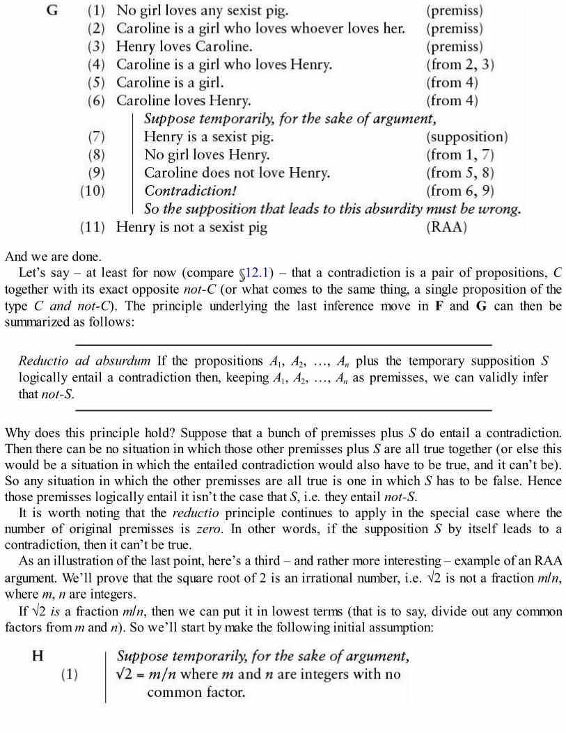
And we are done.Let’s say – at least for now (compare 12.1) – that a contradiction is a pair of propositions, C

together with its exact opposite not-C (or what comes to the same thing, a single proposition of thetype C and not-C). The principle underlying the last inference move in F and G can then besummarized as follows:

Reductio ad absurdum If the propositions A1, A2, …, An plus the temporary supposition Slogically entail a contradiction then, keeping A1, A2, …, An as premisses, we can validly inferthat not-S.

Why does this principle hold? Suppose that a bunch of premisses plus S do entail a contradiction.Then there can be no situation in which those other premisses plus S are all true together (or else thiswould be a situation in which the entailed contradiction would also have to be true, and it can’t be).So any situation in which the other premisses are all true is one in which S has to be false. Hencethose premisses logically entail it isn’t the case that S, i.e. they entail not-S.

It is worth noting that the reductio principle continues to apply in the special case where thenumber of original premisses is zero. In other words, if the supposition S by itself leads to acontradiction, then it can’t be true.

As an illustration of the last point, here’s a third – and rather more interesting – example of an RAAargument. We’ll prove that the square root of 2 is an irrational number, i.e. √2 is not a fraction m/n,where m, n are integers.

If √2 is a fraction m/n, then we can put it in lowest terms (that is to say, divide out any commonfactors from m and n). So we’ll start by make the following initial assumption:

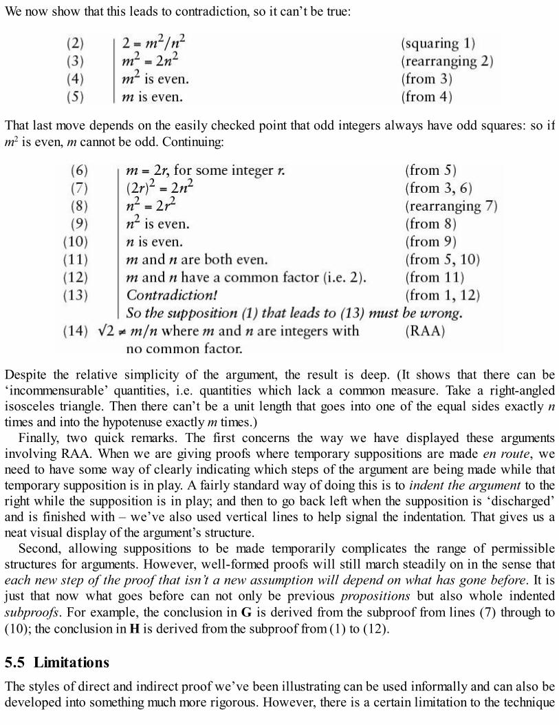
We now show that this leads to contradiction, so it can’t be true:

That last move depends on the easily checked point that odd integers always have odd squares: so ifm2 is even, m cannot be odd. Continuing:

Despite the relative simplicity of the argument, the result is deep. (It shows that there can be‘incommensurable’ quantities, i.e. quantities which lack a common measure. Take a right-angledisosceles triangle. Then there can’t be a unit length that goes into one of the equal sides exactly ntimes and into the hypotenuse exactly m times.)

Finally, two quick remarks. The first concerns the way we have displayed these argumentsinvolving RAA. When we are giving proofs where temporary suppositions are made en route, weneed to have some way of clearly indicating which steps of the argument are being made while thattemporary supposition is in play. A fairly standard way of doing this is to indent the argument to theright while the supposition is in play; and then to go back left when the supposition is ‘discharged’and is finished with – we’ve also used vertical lines to help signal the indentation. That gives us aneat visual display of the argument’s structure.

Second, allowing suppositions to be made temporarily complicates the range of permissiblestructures for arguments. However, well-formed proofs will still march steadily on in the sense thateach new step of the proof that isn’t a new assumption will depend on what has gone before. It isjust that now what goes before can not only be previous propositions but also whole indentedsubproofs. For example, the conclusion in G is derived from the subproof from lines (7) through to(10); the conclusion in H is derived from the subproof from (1) to (12).

5.5 LimitationsThe styles of direct and indirect proof we’ve been illustrating can be used informally and can also bedeveloped into something much more rigorous. However, there is a certain limitation to the technique

of trying to warrant inferences by finding step-by-step proofs. If we are lucky/clever, and spot a proofthat takes us from the given premisses to the target conclusion, that will show that a putative inferenceis indeed valid. But we may be unlucky/dim, and not spot the proof. In the general case, even if aproof exists, proof-discovery requires ingenuity, and failing to find a proof doesn’t show that theoriginal inference from premisses to conclusion is invalid. (Compare the counterexample technique:if we are lucky/ clever, deploying that technique will show us that an invalid inference is invalid. Butwe may miss the counterexample.)

It would be nice to have less hit-and-miss techniques for establishing validity and invalidity.Ideally, we would like a mechanical general technique for working out whether an inference is or isnot valid that doesn’t need any imaginative searching for proofs or counterexamples. Can we ever (asit were) calculate the validity or invalidity of inferences in as mechanical a way as we calculate howmuch five pints of beer will cost, given the price per pint?

Profound results (mostly discovered in the 1930s) show that, in general, a mechanically applicablecalculus will not in fact be available. But in a limited class of cases, we can pull off the trick. In thenext part of this book, starting in Chapter 7, we will be exhibiting one such calculus.

5.6 SummaryTo establish validity we can use many-step deductions, i.e. proofs, which chain together littleinference steps that are obviously valid and that lead from the initial premisses to the desiredconclusion.Some common methods of proof, however, are ‘indirect’, like reductio ad absurdum.In the general case, even if a proof exists, proof-discovery requires ingenuity.

Exercises 5Which of the following arguments are valid? Where an argument is valid, provide a proof. Some ofthe examples are enthymemes that need repair.

1. No philosopher is illogical. Jones keeps making argumentative blunders. No logicalperson keeps making argumentative blunders. All existentialists are philosophers. So,Jones is not an existentialist.

2. Jane has a first cousin. Jane’s father had no siblings. So, if Jane’s mother had no sisters,she had a brother.

3. Every event is causally determined. No action should be punished if the agent isn’tresponsible for it. Agents are only responsible for actions they can avoid doing. Hence noaction should be punished.

4. Something is an elementary particle only if it has no parts. Nothing which has no parts candisintegrate. An object that cannot be destroyed must continue to exist. So an elementaryparticle cannot cease to exist.

5. No experienced person is incompetent. Jenkins is always blundering. No competentperson is always blundering. So, Jenkins is inexperienced.

6. Only logicians are good philosophers. No existentialists are logicians. Someexistentialists are French philosophers. So, some French philosophers are not goodphilosophers.

7. Either the butler or the cook committed the murder. The victim died from poison if the

cook did the murder. The butler did the murder only if the victim was stabbed. The victimdidn’t die from poison. So, the victim was stabbed.

8. Promise-breakers are untrustworthy. Beer-drinkers are very communicative. A man whokeeps his promises is honest. No one who doesn’t drink beer runs a bar. One can alwaystrust a very communicative person. So, no one who keeps a bar is dishonest.

9. When I do an example without grumbling, it is one that I can understand. No easy logicexample ever makes my head ache. This logic example is not arranged in regular order,like the examples I am used to. I can’t understand these examples that are not arranged inregular order, like the examples I am used to. I never grumble at an example, unless itgives me a headache. So, this logic example is difficult.

6

Validity and arguments

Before turning to explore some formal techniques for evaluating arguments, we should pause to say alittle more about the ‘classical’ conception of validity for individual inference steps, and also saymore about what makes for cogent multi-step arguments.

6.1 Classical validity againIn Chapter 1, we introduced the intuitive idea of an inference’s being deductively valid – i.e.absolutely guaranteeing its conclusion, given the premisses. Then in Chapter 2, we gave the classicdefinition of validity, which is supposed to capture the intuitive idea. But does our definition reallydo the trick?

A reminder, and a quiz. We said that an inference is (‘classically’) valid if and only if there is nopossible situation in which the premisses are true and the conclusion false. So consider: according tothat definition, which of the following inferences are classically valid?

A Jo is married; so Jo is married.

B Socrates is a man; Jo is married; all men are mortal; so Socrates is mortal.

C Jack is married; Jack is single; so today is Tuesday.

D Elephants are large; so either Jill is married or she is not.

And then ask: which of the inferences are intuitively deductively compelling? Do your answersmatch?

(1) Trivially, there is no possible way that A’s premiss ‘Jo is married’ could be true and itsconclusion ‘Jo is married’ be false; so the first inference is indeed valid by the classical definition.

What is the intuitive verdict about this argument? Of course, the inference is no use at all as ameans for persuading someone who does not already accept the the conclusion as correct. Still, truth-preservation is one thing, being useful for persuading someone to accept a conclusion is somethingelse (after all, a valid argument leading to an unwelcome conclusion can well serve to persuade itsrecipient of the falsehood of one of the premisses, rather than the truth of the conclusion). Once wemake the distinction between truth-preservation and usefulness, there is no reason not to count the ‘Jo’argument as deductively valid. As we put it in 3.2, an inference that covers no ground hasn’t got achance to go wrong!

Objection: ‘It was said at the very outset that arguments aim to give reasons for their conclusions –and the premiss of A doesn’t give an independent reason for its conclusion, so how can it be a goodargument?’ Reply: Fair comment. We’ve just agreed that A isn’t a persuasive argument, in the sensethat it can’t give anyone who rejects the conclusion a reason for changing their minds. Still, to repeat,

that doesn’t mean that the inferential relation between premiss and conclusion isn’t absolutely secure.And the intuitive idea of validity is primarily introduced to mark absolutely secure inferences: A justillustrates the limiting case where the security comes from unadventurously staying in the same place.

(2) Argument B with a redundant and irrelevant premiss also comes out as valid by the classicaldefinition. There can be no situation in which Socrates is a man, and all men are mortal, yet Socratesis not mortal. So there can be no situation in which Socrates is a man, all men are mortal, and (as ithappens) Jo is married, yet Socrates is not mortal.

What’s the intuitive verdict on B? Well, introducing redundant premisses may be pointless (orworse, may be misleading). But B’s conclusion is still guaranteed, if all the premisses – including theones the really matter – are true.

Generalizing, suppose A1, A2, …, An logically entail C. Then A1, A2, …, An, B logically entail C, forany additional premiss B (both intuitively, and by our official definition).

Deductive inference contrasts interestingly with inductive inference in this respect. Recall the‘coffee’ argument in 1.3:

E (1) Cups of coffee that looked and tasted just fine haven’t killed you in the past.(2) This present cup of coffee looks and tastes just fine.

So (3) This present cup of coffee won’t kill you.

The premisses here probabilistically support the conclusion. But add the further premiss

(2′) The coffee contains a tasteless poison,

and the conclusion now looks improbable. Add the further premiss

(2″) The biscuit you just ate contained the antidote to that poison,

and (3) is supported again (for it is still unlikely the coffee will kill you for any other reason). Thisswinging to and fro of degree of inductive support as further relevant information is noted is onereason why the logic of inductive arguments is difficult to analyse and codify. By contrast, adeductively cogent argument can’t be spoilt by adding further premisses.

(3) So far so good. We can readily live with the results that completely trivial arguments andarguments with redundant premisses count as deductively valid by the classical definition. But nownote that there is no possible situation in which Jack is both married and single. That is to say, there isno possible situation where the premisses of argument C are both true. So, there is no possiblesituation where the premisses of that argument are both true and the conclusion false. So, this timemuch less appealingly, the inference in C also comes out as valid by the classical definition.

The point again generalizes. Suppose that a bunch of propositions A1, A2, …, An is logicallyinconsistent, i.e. there is no possible situation in which A1, A2, …, An are all true together. Then thereis also no situation in which A1, A2, …, An are all true and C is false, whatever C might be. Hence byour definition of classical validity, we can validly infer any proposition we choose from a bunch ofinconsistent premisses.

That all looks decidedly counter-intuitive. Surely the propositions ‘Jack is married’ and ‘Jack is

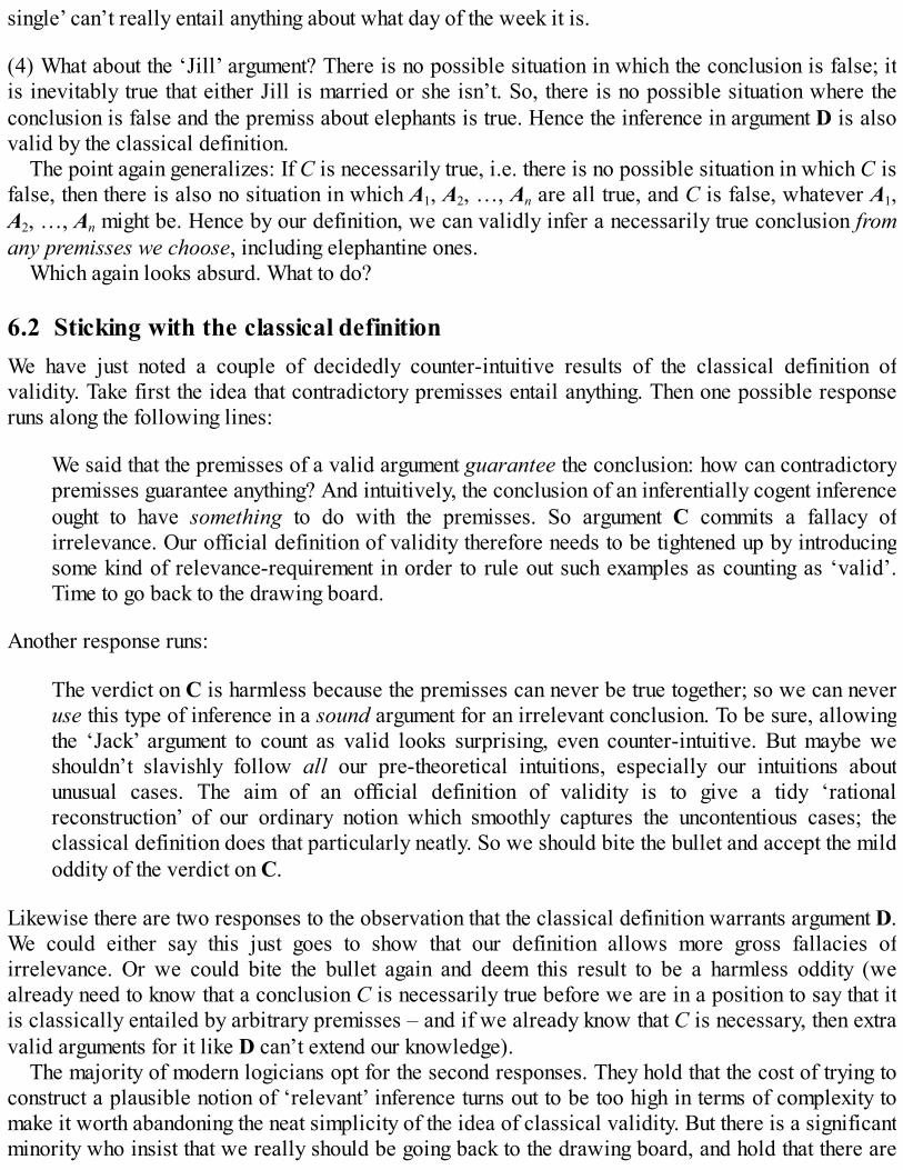
single’ can’t really entail anything about what day of the week it is.

(4) What about the ‘Jill’ argument? There is no possible situation in which the conclusion is false; itis inevitably true that either Jill is married or she isn’t. So, there is no possible situation where theconclusion is false and the premiss about elephants is true. Hence the inference in argument D is alsovalid by the classical definition.

The point again generalizes: If C is necessarily true, i.e. there is no possible situation in which C isfalse, then there is also no situation in which A1, A2, …, An are all true, and C is false, whatever A1,A2, …, An might be. Hence by our definition, we can validly infer a necessarily true conclusion fromany premisses we choose, including elephantine ones.

Which again looks absurd. What to do?

6.2 Sticking with the classical definitionWe have just noted a couple of decidedly counter-intuitive results of the classical definition ofvalidity. Take first the idea that contradictory premisses entail anything. Then one possible responseruns along the following lines:

We said that the premisses of a valid argument guarantee the conclusion: how can contradictorypremisses guarantee anything? And intuitively, the conclusion of an inferentially cogent inferenceought to have something to do with the premisses. So argument C commits a fallacy ofirrelevance. Our official definition of validity therefore needs to be tightened up by introducingsome kind of relevance-requirement in order to rule out such examples as counting as ‘valid’.Time to go back to the drawing board.

Another response runs:

The verdict on C is harmless because the premisses can never be true together; so we can neveruse this type of inference in a sound argument for an irrelevant conclusion. To be sure, allowingthe ‘Jack’ argument to count as valid looks surprising, even counter-intuitive. But maybe weshouldn’t slavishly follow all our pre-theoretical intuitions, especially our intuitions aboutunusual cases. The aim of an official definition of validity is to give a tidy ‘rationalreconstruction’ of our ordinary notion which smoothly captures the uncontentious cases; theclassical definition does that particularly neatly. So we should bite the bullet and accept the mildoddity of the verdict on C.

Likewise there are two responses to the observation that the classical definition warrants argument D.We could either say this just goes to show that our definition allows more gross fallacies ofirrelevance. Or we could bite the bullet again and deem this result to be a harmless oddity (wealready need to know that a conclusion C is necessarily true before we are in a position to say that itis classically entailed by arbitrary premisses – and if we already know that C is necessary, then extravalid arguments for it like D can’t extend our knowledge).

The majority of modern logicians opt for the second responses. They hold that the cost of trying toconstruct a plausible notion of ‘relevant’ inference turns out to be too high in terms of complexity tomake it worth abandoning the neat simplicity of the idea of classical validity. But there is a significantminority who insist that we really should be going back to the drawing board, and hold that there are

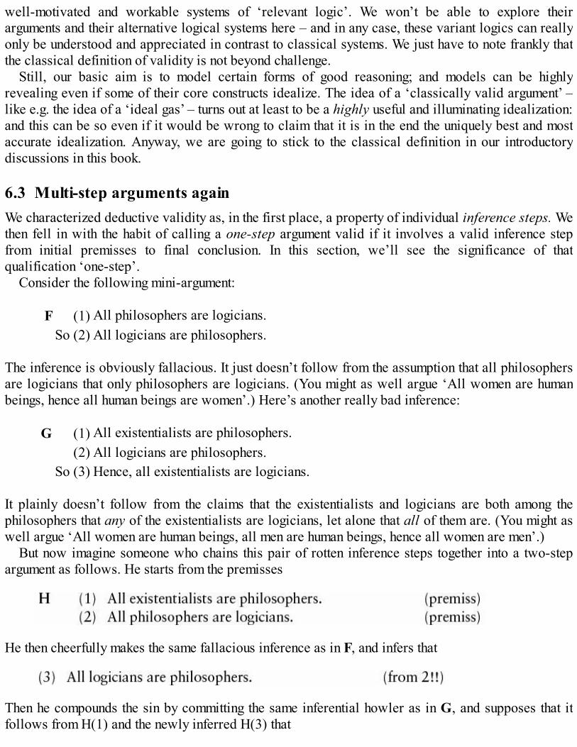
well-motivated and workable systems of ‘relevant logic’. We won’t be able to explore theirarguments and their alternative logical systems here – and in any case, these variant logics can reallyonly be understood and appreciated in contrast to classical systems. We just have to note frankly thatthe classical definition of validity is not beyond challenge.

Still, our basic aim is to model certain forms of good reasoning; and models can be highlyrevealing even if some of their core constructs idealize. The idea of a ‘classically valid argument’ –like e.g. the idea of a ‘ideal gas’ – turns out at least to be a highly useful and illuminating idealization:and this can be so even if it would be wrong to claim that it is in the end the uniquely best and mostaccurate idealization. Anyway, we are going to stick to the classical definition in our introductorydiscussions in this book.

6.3 Multi-step arguments againWe characterized deductive validity as, in the first place, a property of individual inference steps. Wethen fell in with the habit of calling a one-step argument valid if it involves a valid inference stepfrom initial premisses to final conclusion. In this section, we’ll see the significance of thatqualification ‘one-step’.

Consider the following mini-argument:

F (1) All philosophers are logicians.So (2) All logicians are philosophers.

The inference is obviously fallacious. It just doesn’t follow from the assumption that all philosophersare logicians that only philosophers are logicians. (You might as well argue ‘All women are humanbeings, hence all human beings are women’.) Here’s another really bad inference:

G (1) All existentialists are philosophers.(2) All logicians are philosophers.

So (3) Hence, all existentialists are logicians.

It plainly doesn’t follow from the claims that the existentialists and logicians are both among thephilosophers that any of the existentialists are logicians, let alone that all of them are. (You might aswell argue ‘All women are human beings, all men are human beings, hence all women are men’.)

But now imagine someone who chains this pair of rotten inference steps together into a two-stepargument as follows. He starts from the premisses

He then cheerfully makes the same fallacious inference as in F, and infers that

Then he compounds the sin by committing the same inferential howler as in G, and supposes that itfollows from H(1) and the newly inferred H(3) that

Here our reasoner has got from the initial premisses H(1) and H(2) to his final conclusion H(4) bytwo quite terrible moves: it would therefore be extremely odd to dignify his supposed ‘proof’ asdeductively cogent.

Note, however, that in this case the two howlers by luck happen to cancel each other out; there areno possible circumstances in which the initial premisses H(1) and H(2) are both true and yet the finalconclusion H(4) is false. If the existentialists are all philosophers, and all philosophers are logicians,then the existentialists must of course be logicians. Hence, the inferential jump from initial premissesto final conclusion is in fact valid.

So if we were to say (without any qualification) that an argument is valid if the initial premissesabsolutely guarantee the final conclusion, then we’d have to count the two-step argument H as ‘valid’.Which is, to say the least, a very unhappy way of describing the situation, given that H involves acouple of nasty fallacies!

The previous chapter reminds us that many arguments involve more than one inference step. To besure, we don’t very often set them out as semi-formal proofs; but multi-step arguments are commonenough in any form of extended enquiry – indeed our initial informal definition of an argument ( 1.1)was as a chain of reasoning. The point of multi-step chains is to show that you can legitimately infersome (perhaps highly unobvious) conclusion by breaking down the big inferential leap from initialpremisses to final conclusion into a series of smaller, more evident steps. But if an argument goesastray along the way, then it will be mere good luck if it happens to get back on track to a conclusionthat does genuinely follow via some other route from the starting premisses.

The moral here is a simple one: we need to make a distinction. Suppose we have a step-by-stepargument from premisses A1, A2, …, An to conclusion C. Then it is one thing to say that the overall,big-leap, inference from A1, A2, …, An to C is valid. It is another thing to say that the argument wegive from A1, A2, …, An to C is deductively cogent. Of course, in the case where the argument hasonly one step, then the argument is deductively cogent if and only if the overall inference is valid. Butas example H shows, in the case of multi-step arguments, this two-way link breaks down. Theinferential leap from the premisses to conclusion might still be valid, even if some step-by-stepargument we give to defend the inference is not deductively cogent.

You might think that we are making much ado about very little here. For doesn’t this just show thatwe must define a genuine proof – a deductively virtuous multi-step argument, where luck doesn’tenter into it – to be an argument whose individual inferential steps are all valid? (In fact, that wasour first-shot definition in 5.1.)

But things aren’t quite that easy. Not only must individual steps be valid, but they must be chainedtogether in the right kind of way.

To illustrate, consider this one-step inference:

I (1) Socrates is a philosopher.(2) All philosophers have snub noses.

So (3) Socrates is a philosopher and all philosophers have snub noses.

That’s trivially valid (if you are given A and B, you can infer A-and-B). Here is another equallytrivial but valid inference:

J (1) Socrates is a philosopher and all philosophers have snub noses.So (2) All philosophers have snub noses.

From A-and-B, you can infer B. And thirdly, this too is plainly valid:

K (1) Socrates is a philosopher.(2) All philosophers have snub noses.

So (3) Socrates has a snub nose.

Taken separately, then, those three little inferences are quite unproblematic. But now imaginesomeone chains them together, not in the usual way (where each step depends on something that hasgone before) but in the following tangle:

By separately valid steps we seem to have deduced the shape of Socrates’ nose just from the premissthat he is a philosopher! What has gone wrong?

The answer is obvious enough. In the middle of the argument we have gone round in a circle. L(2)is derived from L(3), and then L(3) is derived from L(2). Circular arguments can’t take us anywhere.

So that suggests we need an improved account of what makes for a deductively cogent proof: theindividual inferential steps must all be valid, and the steps must be chained together in a non-circularway, with steps only depending on what’s gone before in the argument.

That’s an improvement, but more still needs to be said. For recall, we need to allow for multi-steparguments like the ‘reductio’ arguments we met in 5.4 – i.e. arguments where we can introduce a newtemporary supposition that doesn’t follow from what’s gone before (and then later ‘discharge’ theassumption by an inference step that relies, not on prior propositions, but on a prior ‘sub-proof’).Then there will be more complications when we introduce ‘downward-branch-ing tree proofs’ (see 20.1). Recognizing such various argument-styles as all being in good order complicates the task offraming a definition of what makes for a deductively cogent proof in general. Fortunately, for ourpurposes in this book, we don’t need to come up with a general story here: so we won’t attempt to doso.

6.4 SummaryOur classical definition of validity counts as valid any inference which has inconsistentpremisses, or has a necessarily true conclusion. Despite being counter-intuitive, these areupshots we will learn to live with.It is unhappy to say that a multi-step argument is ‘valid’ just if there is no way the initialpremisses can be true and the conclusion false. For we don’t want to endorse arguments wherethere are inferential steps which are invalid but where it happens that the fallacies cancel each

other out.

Interlude

Logic, formal and informal

What has been covered so far?

We have explained, at least in an introductory way, the notion of a classically valid inference-step.We have explained the corresponding notion of a deductively valid one-step argument.We have distinguished deductive validity from other virtues that an argument might have (likebeing a good inductive argument).We have noted how different arguments may share the same pattern of inference. And weexploited this fact when we developed the counterexample technique for demonstratinginvalidity.We have seen some simple examples of direct and indirect multi-step proofs, where we showthat a conclusion really can be validly inferred from certain premisses by filling in the gapbetween premisses and conclusion with evidently valid intermediate inference steps.

What haven’t we done so far?

We still haven’t given a very sharp characterization of the notion of deductive validity (weinvoked an intuitive notion of ‘possible situation’ without really spelling out what that came to).Nor have we given a really clear story about what counts as a ‘pattern’ of inference.Nor have we given a sharp characterization of what counts as a legitimate ‘well-built’ form ofmulti-step proof.Indeed, we even set aside the question of the nature of the basic constituents of informalarguments, namely propositions (so in a sense, we don’t really know the first thing about validarguments, i.e. what they are made of).

At this point, then, we could go in a number of directions. We could remain content with an informallevel of discussion, and first explore more techniques for teasing out the inferences involved in real-life passages of extended prose argumentation. Then we could explore a variety of ways of evaluatinga wide range of everyday deductions. We could also turn our attention to various inductive,probabilistic modes of argument, and explore the sorts of fallacies we can fall into when trying toargue inductively. And that kind of wide-ranging study in informal logic (as it is often called) wouldbe a highly profitable enterprise. But this book takes a different direction. We are going to presupposethat we are already moderately competent at filleting out the bones of an argument from everydayprose; and we are going to be focusing on just a couple of broad classes of deductive inferences, withthe aim of constructing rigorous, comprehensive, formal theories about them.

We are going, in short, for depth rather than breadth. Our approach will give us a powerful set of

tools for dealing with certain kinds of real-life arguments. But that isn’t the only reason for taking theformal route. For just as in-depth theories about genes or electrons tell us what genes and electronsreally are, we might hope that these rigorous theories about some core types of argument will tell usmore about what validity for such arguments amounts to. Moreover, in the course of these discussionswe are going to be developing a range of other ideas which belong in the toolkit of any analyticphilosopher.

I’d claim, in fact, that the now well understood theory of ‘first-order quantification theory’ – themain branch of formal logic which we are introducing in this book – is one of the great intellectualachievements of twentieth-century logicians. It opens the door into a rich and fascinating field: andalthough, in this introductory book, there will only be occasional glimpses through the door, whatfollows will take us right to the threshold.

There are, however, different possible routes to the threshold, different (though ultimatelyequivalent) ways of starting to develop formal logical systems. Once upon a time, so-calledaxiomatic systems were the fashion. More recently, most students were introduced to serious logicvia some sort of ‘natural deduction’ system. More recently still, systems using ‘tree’ proofs havebecome popular, being particularly easy to understand and manipulate by those without amathematical bent. Given world enough and time, we’d develop all three main approaches, anddiscuss their pros and cons. But done in enough detail, that survey would take too long; and donequickly, it would just confuse beginners. We have to choose. So this book chooses to introduce formallogic by trees. What that involves will become clear soon enough.

7

Three propositional connectives

In the next part of the book, we will be concentrating on a very restricted class of inferences, whoselogical structure involves the so-called propositional connectives, ‘and’, ‘or’ and ‘not’. Sucharguments may not be very exciting in themselves: but the exercise of developing systematictechniques for evaluating them is the simplest way of introducing a number of the centrally importantconcepts and strategies of formal logic. This present chapter explains the advantages of introducing aformalized language in which to express arguments involving the propositional connectives.

7.1 ‘And’, ‘or’ and ‘not’Consider the following argument:

A (1) Either we are out of petrol or the carburettor is blocked.(2) We are not out of petrol.

So (3) The carburettor is blocked.

That argument is valid; so is this one:

A′ (1) Either Jill is in the library or she is in the coffee bar.(2) Jill isn’t in the library.

So (3) Jill is in the coffee bar.

Evidently, we can generalize here. Our two arguments have the form

Either A or BNot ASo, B

And any inference sharing the same form will be valid.Three quick comments about this. First, we are here using ‘A’ and ‘B’ to stand in for whole

propositions, such as ‘We are out of petrol’ or ‘Jill is in the coffee bar’. We can call these(schematic) propositional variables. We have used such propositional variables before (e.g. in 3.3and 5.4): contrast the use of ‘F’ and ‘G’ which schematically represent predicates, and ‘n’ whichholds the place of a naming or subject term.

Second, what about our representation of the form of the second premiss in each case? We havewritten Not A. But the premiss ‘We are not out of petrol’ does not begin with ‘not’. Still, inserting the‘not’ into ‘We are out of petrol’ has the result of denying what was asserted by the original sentence.

And we can very naturally represent the proposition which says exactly the opposite of A by Not A.Third, note that in representing the structure of the second argument we have ignored the surface

difference between using the name ‘Jill’ and using the pronoun ‘she’ to refer to Jill. You might say thatwe are trying to represent logical structure, not just surface form (see 3.5).

Here’s another pair of valid arguments:

B (1) It’s not the case that Jack played lots of football and also did well in his exams.(2) Jack played lots of football.

So (3) Jack did not do well in his exams.

B′ (1) It’s not true that Tony supports the policy and George does too.(2) Tony supports the policy.

So (3) George does not support it.

These two evidently share the same reliable inferential form, which we might represent as follows:

Not (A and B)ASo, not B

In each case, the first premiss says that something is not the case, where the something in question is acombination of two propositions linked by ‘and’. Why use brackets in representing this structure?Well, we certainly do want to distinguish

Not (A and B)

– which joins together A and B, and then says that this combination doesn’t hold – from

(Not-A and B)which denies A, but then adds that B does hold. For suppose we replace

A: The President orders an invasion.B: There will be devastation.

Then Not (A and B) represents the hopeful thought that it isn’t true that the President will order aninvasion with consequent devastation; while (Not-A and B) is the distinctly less cheering claim thatalthough the President will not order an invasion, there will still be devastation all the same.

We have seen, then, two examples of valid inference patterns where the relevant logical materialsare simply ‘and’ ‘or’ and ‘not’. Here is a patently invalid inference:

C (1) It is not the case that Alice is clever and Bob is clever too.So (2) Alice is not clever.

Suppose Alice is clever but Bob is a dunce: then the premiss is true and the conclusion false in thatsituation. More generally; from Not (A and B) you can’t in general infer Not A – for maybe B is toblame for the falsity of (A and B).

These initial examples are extremely trite; but they give us some first cases of arguments whosevalidity or invalidity depends on the distribution among the premisses and conclusion of the threepropositional connectives ‘and’ ‘or’ and ‘not’.

Talk of ‘connectives’ here is obviously apt for ‘and’ and ‘or’. Thus ‘and’ connects two propositionsA, B to give us the more complex proposition A and B. Likewise ‘or’ connects two propositions A, Bto give us the more complex proposition A or B. It is a bit stretched to call ‘not’ a connective, since itoperates on just one proposition and (so to speak) turns it on its head. Still, ‘not’ is like ‘and’ and ‘or’in giving us a way of building more complex propositions from simpler ones (and we will soondiscover some closer similarities). So we will follow convention and count ‘not’ as an honoraryconnective.

We are going to explore, then, arguments involving these three propositional connectives; and laterwe will present a mechanical way of demonstrating validity for such arguments. But before getting tothat point, a fair amount of preliminary but important ground-clearing needs to be done.

7.2 Quirks of the vernacularLet’s remark briefly on some of the complexities and quirks of ‘and’, ‘or’ and ‘not’ as they function invernacular English.

(1) We can use ‘and’ to conjoin a pair of matched expressions belonging to almost any grammaticalcategory – as in ‘Jack is fit and tanned’, ‘Jill won quickly and easily’, ‘Jack and Jill went up the hill’,or ‘Jo smoked and coughed’, where ‘and’ conjoins respectively pairs of adjectives, adverbs, propernames and verbs. But set aside all those uses, and consider only the cases where ‘and’ joins twowhole sentences to form a new one. In most such cases what we get is a sentence which expresses thebare conjunction of the propositions expressed by the original sentences:

The conjunction of two propositions A and B is true when A and B are both true, and is falseotherwise.

However, inserting an ‘and’ between two claims in English doesn’t always express their bareconjunction. Take the two claims

(a) There is not a word of truth in the reports that Jill loves Jack.(b) Jack loves Jill.

Perhaps both these are true: Jack’s love is sadly unrequited. But you could hardly assert this just bysticking an ‘and’ between (a) and (b). For that yields

(c) There is not a word of truth in the reports that Jill loves Jack and Jack loves Jill,

which is naturally heard as denying (b) rather than as asserting it! Mechanically gluing together twoclaims with ‘and’ isn’t an infallible way of arriving at their conjunction.

There is another kind of complication: compare

(d) Eve became pregnant and she married Adam.(e) Eve married Adam and she became pregnant.

These are naturally taken as conveying different messages about temporal order. Does ‘and’ inEnglish therefore sometimes mean more than bare conjunction and connote, e.g., temporal successionas well? It might appear so.

But perhaps appearances deceive. For delete the ‘and’ from (d), take what is left as two separatesentences, and the implication of temporal succession still remains because of our default narrativepractice of telling a story in the order the events happened. Since the implication remains evenwithout the use of the connective ‘and’, there is perhaps no need to treat temporal succession as onepossible meaning of the connective itself.

However, we won’t pursue that debate further. The point is that there is at least an issue here aboutwhether ‘and’ sometimes means more than pure conjunction.

(2) Turning next to ‘or’, we can again use this connective to combine a pair of matched expressionsbelonging to almost any grammatical category – as in ‘Jack is cycling or driving’, ‘Jack or Jill wentup the hill’, and so forth. But set aside all those uses, and consider only the cases where ‘or’ is usedto join two whole propositional clauses. The obvious complication here is that sentences of the kindA or B can often be heard as meaning A or B but not both (‘Either you will hand your logic exercisesin by midday or you will have to leave the class’; ‘Either a peace treaty will be signed this week orthe war will drag on another year’). But about equally often, such sentences can be heard as meaningA or B or perhaps both (of a student with bad grades, I say ‘Either he didn’t try, or he really isn’t anygood at logic’).

Those two readings of ‘or’ are called the ‘exclusive’ and ‘inclusive’ readings respectively. So:

The exclusive disjunction of two propositions A and B is true when exactly one of A and B istrue, and is false otherwise.

The inclusive disjunction of two propositions A and B is true when at least one of A and B istrue, and is false otherwise.

If we are going to consider the logic of ‘or’, then we will need for a start to have some explicit wayof signalling when we are dealing with exclusive disjunctions and when we are dealing withinclusive cases.

(3) The complexities in the behaviour of ‘not’ are different again. What concerns us here is theoperation which yields the negation of a proposition, which says the exact opposite of the originalproposition:

The negation of a proposition A is true exactly when A is false and is false exactly when A istrue.

In English we can often negate a claim by inserting the word ‘not’ at an appropriate place and thenmaking any required grammatical adjustments. Thus the negation of ‘Jo is married’ is ‘Jo is not

married’, and the negation of ‘Jack smokes’ is ‘Jack does not smoke’.But contrast: inserting a ‘not’ into the truth ‘Some students are good logicians’ at the only

grammatically permissible place in fact gives us another truth, namely ‘Some students are not goodlogicians’. Hence, inserting ‘not’ isn’t always sufficient to produce the negation of a proposition. Noris it always necessary (for example, replacing ‘some’ by ‘no’ in ‘Some students are good logicians’does give us the negation).

It might be supposed that English does have a cumbersome but sure-fire way of forming negations,namely prefixing a sentence with the phrase ‘It is not the case that’. For example, ‘It is not the casethat some students are good logicians’ is indeed the negation of ‘Some students are good logicians’.And this works in nearly every case. But not always. Compare

(f) Jack loves Jill and it is not the case that Jill loves Jack.(g) It is not the case that Jack loves Jill and it is not the case that Jill loves Jack.

Here, (g) results from prefixing ‘It is not the case that’ to (f). Yet on the natural readings, both (f) and(g) are false if Jack and Jill love each other; so these two sentences don’t express propositions whichare real contradictories. In fact, (g) is naturally read as having the form (Not-A and Not-B) – whilethe real negation of (f) would need to have the form Not (A and Not-B).

(4) Finally, let us note that English sentences which involve more than one connective can beambiguous. Consider

(h) Either Jack took Jill to the party or he took Jo and he had some fun.

Does this say that Jack went to the party with Jo and had fun, or else he went with Jill. Or does it say,differently, that he took Jill or Jo to the party and either way enjoyed himself?

Logicians talk about the scope of connectives (and other logical operators). For example, in thenatural reading of (g), the scope or ‘coverage’ of the first ‘It is not the case that’ is just the next clause,‘Jack loves Jill’. In (h), however, there is an ambiguity of scope, i.e. an ambiguity in how to grouptogether the clauses. Thus what is the scope of the ‘and’? Does it (first reading) just conjoin ‘he tookJo’ and ‘he had some fun’? Or is the scope or ‘coverage’ wider (second reading), so that the whole of‘either Jack took Jill to the party or he took Jo’ is being conjoined with ‘he had some fun’?

7.3 FormalizationEven the handful of examples in the previous section is enough to establish that natural-languageconnectives can behave in some rather quirky and ambiguous ways. The same goes for other logicallysalient constructions (as we will see later, for example, when discussing expressions like ‘all’ and‘any’ in 21.1). So to treat the logic of arguments couched in ordinary English really requires takingon two tasks simultaneously; we need both to clarify the many vagaries of English and to deal withthe logical relations of the messages variously expressible in the language.

Given our interest is in logic rather than linguistics, is there a way to divide the labour?Here is a very inviting, though radical, strategy. We can bulldoze past many of the problems

generated by the quirkiness of natural language if, instead of using the messy vernacular to expressarguments, we use some much more austere and regimented formal language which is designed to be

logically well-behaved and quite free of ambiguities and shifting meanings. We then assess argumentsinvolving (for instance) the English ‘and’, ‘or’ and ‘not’ by a two-step process. We start by (1)rendering the vernacular argument into a well-behaved artificial language; and then (2) we investigatethe validity or otherwise of the reformulated argument. Step (1) of this two-step process may raiseissues of interpretation: but as logicians we can largely focus on step (2). For even given thepremisses and conclusion translated into a perspicuous and unambiguous notation, the centralquestion of how to assess the argument for validity remains.

This two-step strategy has its roots as far back as Aristotle who used Greek letters as symbols inpresenting syllogisms. But the strategy came of age in the nineteenth century with the German logicianGottlob Frege (who wrote works such as the Begriffsschrift which presented a ‘concept-script’designed for the perspicuous representation of propositions). Frege was soon followed by, amongothers, Bertrand Russell and A. N. Whitehead early in the last century: their monumental PrincipiaMathematica aims to derive core chunks of classical mathematics from a tiny handful of axioms. Andin order to enforce total precision, the derivations are couched not in the informal mix of English andsymbols that mathematicians usually use, but in an artificial symbolic language.

In the rest of this book, we are going to follow this two-step strategy, which really underlies thewhole project of modern formal logic. The defence of this strategy is its abundant fruitfulness, andthat can only become fully clear as we go along. At this stage, therefore, you’ll have to take it on trustthat the (small) effort required in mastering some simple formal languages will pay off handsomely.

7.4 The design brief for PLFor our immediate purposes, then, we want to design an appropriate language for regimentingarguments involving conjunction, disjunction and negation, a language which must avoid the quirksand ambiguities of ordinary language.

PL (the label is supposed to suggest ‘Propositional Logic’) is a set of symbolic devices designedto do this job in an entirely straightforward and simple way. We can usefully carve up its design briefinto three parts.

(1) First, we want symbols for the three connectives.

So we give PL a connective ‘∧’ which is stipulated invariably to signify bare conjunction, nomore and no less: i.e. (A ∧ B) is always to be true just when A and B are both true.We add a connective ‘∨’ which is stipulated invariably to signify inclusive disjunction, nomore and no less (we will see later how to deal with exclusive disjunction in PL). So (A ∨ B)is always to be true just when A is true or B is true or both. ‘∨’ is often read vel, which is Latinfor inclusive ‘or’.Finally we add a negation prefix ‘¬’ which always works as the English ‘It is not the case that’usually works; i.e. ¬A invariably expresses the strict negation of A, and is true just when A isfalse.

By all means, read ‘∧’, ‘∨’ and ‘¬’ aloud as respectively ‘and’, ‘or’ and ‘not’ – but remember toothat these new symbols shouldn’t be thought of as mere abbreviations of their ordinary-languagereadings. For mere abbreviations would inherit the ambiguities of their originals, and then whatwould be the point of introducing them? These PL connectives are better thought of as cleaned-up

replacements for the vernacular connectives, which unambiguously express their originals’ coremeanings.

(2) Next, we want to avoid any structural scope ambiguities as in ‘Either Jack took Jill to the party orhe took Jo and he had a really good time’. So ambiguous expressions of the type A ∨ B ∧ C must bebanned. How should we achieve this? Compare arithmetic, where again we can form potentiallyambiguous expressions like ‘1 + 2 × 3’ (is the answer 7 or 9?). Here we can disambiguate by usingbrackets, and write either ‘(1 + (2 × 3))’ and ‘((1 + 2) × 3)’, which both have unique values. We’lluse the same simple device in PL. That is to say, we’ll insist on using brackets, and write either (A ∨(B ∧ C)) or ((A ∨ B) ∧ C). So, more generally:

every occurrence of ‘∧’ and ‘∨’ is to come with a pair of brackets to indicate the scope of theconnective, i.e. to demarcate exactly the limits of what they are connecting;but since the negation sign ‘¬’ only combines with a single sentence, we don’t need to usebrackets with that.

The convention, then, is that (roughly speaking) the negation sign binds tightly to the PL clause thatimmediately follows it. So:

in a sentence of the form (A ∨ (¬B ∧ C)), just B is being negated;in (A ∨ ¬(B ∧ C)), all the bracketed conjunction (B ∧ C) is negated;and in ¬(A ∨ (B ∧ C)), the whole of (A ∨ (B ∧ C)) is negated.

(3) Finally, what do these three connectives ‘∧’, ‘∨’ and ‘¬’ (ultimately) connect? Some simple,connective-free, sentences of the language. So we’ll need to give PL a base class of items whichexpress propositional messages: we can think of these as the atoms of an artificial language. Since forpresent purposes we are not interested in further analysing what is conveyed by these atomicsentences – we are concentrating on the logical powers of ‘and’, ‘or’ and ‘not’ when they connectwhole sentences – we might as well waste as little ink as possible and just use single letters for them.So, for maximum brevity, the single letters ‘P’, ‘Q’, ‘R’, ‘S’ can serve as atoms for the language.(Though, since we could well want to use more than four atoms, we’ll also allow ourselves to cookup as many more as we need by adding ‘primes’ to yield ‘P′’, ‘P′′’, ‘Q′′′′’, etc.)

And that’s all we need. So, by way of interim summary: PL has a base class of symbols whichexpress whole ‘atomic’ propositional messages, and which might as well be as simple as possible.More complex, ‘molecular’, symbolic formulae are then built up using ‘∧’, ‘∨’ and ‘¬’, bracketingvery carefully as we go. And since PL is purpose-designed for expressing arguments whose relevantlogical materials are just conjunction, disjunction and negation and no more, that is all the structurewhich we need to give the language.

7.5 Some simple examplesSuppose we adopt the following translation key:

‘P’ means Jack loves Jill.‘Q’ means Jill loves Jack.‘R’ means Jo loves Jill.

‘S’ means Jack is wise.

Let’s render the following into PL (even with our very quick explanations so far, these should notcause too much trouble: so try your hand at the translations before reading on).

1. Jack doesn’t love Jill.2. Jack is wise and he loves Jill.3. Either Jack loves Jill or Jo does.4. Jack and Jill love each other.5. Neither Jack loves Jill nor does Jo.6. It is not the case that Jack loves Jill and it is not the case the Jill loves Jack.7. Either Jack is not wise or both he and Jo love Jill.8. It isn’t the case that either Jack loves Jill or Jill loves Jack.

The first four are indeed done very easily:

1′. ¬P2′. (S ∧ P)3′. (P ∨ R)4′. (P ∧ Q)

Just three comments. First remember that we are insisting that whenever we introduce an occurrenceof ‘∧’ or ‘∨’, there needs to be a pair of matching brackets to indicate the scope of the connectives.To be sure, the brackets in (2′) to (4′) are strictly speaking redundant; if there is only one connectivein a sentence, there is no possibility of a scope ambiguity needing to be resolved by bracketing. Nomatter, our bracketing policy will be strict. Second, note that rendering the English as best we caninto PL isn’t a matter of mere phrase-for-phrase transliter-ation or mechanical coding. For example,in rendering (2) we have to assume that the ‘he’ refers to Jack; likewise we need to read (3) as sayingthe same as ‘either Jack loves Jill or Jo loves Jill’ – and assume too that the disjunction here isinclusive. Third, note that it is customary not to conclude sentences of our mini-language PL by fullstops.

To continue. We don’t have a ‘neither …, nor …’ connective in PL. But we can translate (5) in twoequivalent ways:

5′. ¬(P ∨ R)5′′. (¬P ∧ ¬R)

(Convince yourself that these renditions do come to the same.)The natural reading of (6), as remarked in 7.2, treats it as the conjunction of ‘It is not the case that

Jack loves Jill’ and ‘It is not the case the Jill loves Jack’; so translating into PL we get:

6′. (¬P ∧ ¬Q)

And the next proposition is to be rendered as follows:

7′. (¬S ∨ (P ∧ R))

(Check you see why the brackets need to be placed as they are.) Finally, we have

8′. ¬(P ∨ Q)

So far, so simple. But now we’ve got going, we can translate ever more complicated sentences.For example, consider

9. Either Jack and Jill love each other or it isn’t the case that either Jack loves Jill orJill loves Jack.

This is naturally read as the disjunction of (4) and (8); so we translate it by disjoining the translationsof (4) and (8), thus:

9′. ((P ∧ Q) ∨ ¬(P ∨ Q))

If we want to translate the negation of (9), we write

10′. ¬((P ∧ Q) ∨ ¬(P ∨ Q))

And so it goes.In the next chapter we will begin characterizing PL rather more carefully. This won’t involve any

major new ideas; the aim will be to be maximally clear and careful about what is going on. Butbefore plunging into those details, let’s just summarize again why we are engaging in this enterprise.

7.6 SummaryThere is a class of inferences whose validity (or invalidity) depends on the way conjunction,disjunction, and negation feature in the premisses and conclusion.‘And’, ‘or’ and ‘not’ in English are used to express conjunction, disjunction, and negation; butthere are many quirks and ambiguities in the way ordinary language expresses these logicaloperations.So to avoid the quirks of the vernacular, we are going to use a special-pur-pose language PL toexpress arguments whose relevant logical materials are the connectives ‘and’, ‘or’ and ‘not’.The design brief for PL is for the simplest language to do this without any ambiguities orobscurities.

Exercises 7A The strict negation of a proposition can usually be expressed by prefixing the operator ‘It is not the

case that’. Can you think of any exceptions in addition to the kind described in 7.2? Can you thinkof further cases which suggest that ‘and’ in English might sometimes mean more than bareconjunction?

B What is the most natural way in English of expressing the strict negations of the following?

1. No one loves Jack.2. Only unmarried men love Jill.3. Everyone who loves Jack admires Jill.4. Someone loves both Jack and Jill.5. Jill always arrives on time.6. Whoever did that ought to be prosecuted.7. Whenever it rains, it pours.8. No one may smoke.

C Two propositions are contraries if they cannot be true together; they are contradictories if one istrue exactly when the other is false. (Example: ‘All philosophers are wise’ and ‘No philosophersare wise’ are contraries – they can’t both be true. But maybe they are both false, so they are notcontradic-tories.) Give examples of propositions which are contraries but not contradictories of B1–7.

D Using the same translation manual as in 7.5, render the following into PL:

1. Jack is unwise and loves Jill.2. It isn’t true that Jack doesn’t love Jill.3. Jack loves Jill and Jo doesn’t.4. Jack doesn’t love Jill, neither is he wise.5. Either Jack loves Jill or Jill loves Jack.6. Either Jack loves Jill or Jill loves Jack, but not both.7. Either Jack is unwise or he loves Jill and Jo loves Jill.

8

The syntax of PL

In the previous chapter, we explained why it is advantageous to introduce an artificial language PL inwhich to express arguments involving conjunction, disjunction and negation. In this chapter, we’lldescribe the structure of our new language much more carefully.

8.1 Syntactic rules for PLThe grammar or syntax of PL determines which strings of symbols count as potentially meaningfulsentences of the language. In other words, to use the standard terminology, the syntax defines whatcounts as a well-formed formula of the language – henceforth ‘wff’ for short.

First, then, we specify which symbols form the basic building blocks for individual wffs:

The basic alphabet of PL is: P, Q, R, S, ′, ∧, ∨, ¬, (, ).

Later, we will want to string wffs together into arguments, and for those purposes it is useful to havethree more symbols, a comma (to separate wffs in lists of premisses), an inference marker (the PLanalogue of ‘therefore’), and an absurdity marker (meaning ‘Contradiction!’). So let’s add them to theofficial alphabet straight away. Hence,

The full alphabet of PL is the comma, plus: P, Q, R, S, ′, ∧, ∨, ¬, (, ), ∴, .

Now we must specify which strings of symbols from the basic alphabet form atomic wffs. Asexplained, we will set the atomic wffs to be as simple as possible:

P, Q, R, S, P′, Q′, R′, S′, P″, Q″, ….

But how are we supposed to continue the sequence here? We want to be absolutely precise: thereshould be no obscurity or vagueness about what does or doesn’t belong to the set of atomic wffs, soan open-ended list won’t really do. On the other hand, we can’t just list a few more atoms and thenstop, since we don’t want to put an arbitrary finite bound on the size of this set (if there were e.g. just14 atoms, we couldn’t use PL to encode an argument that involved 15 different propositionalcomponents). So, more formally, we will define the set of atomic wffs as follows:

(A1) ‘P’, ‘Q’, ‘R’ and ‘S’ are atomic wffs.(A2) Any atomic wff followed immediately by a prime ‘′’ is an atomic wff.(A3) Nothing is an atomic wff other than what can be shown to be so by the rules (A1) and

(A2).

By (A1) and (A2), ‘P′’ is an atomic wff; and then repeatedly applying (A2) again shows that ‘P′′’, ‘P′′′’, etc. are atomic wffs. (By the way, a rule like this, which can be reapplied to the results of its ownprevious application is standardly called recursive.) So (A1) and (A2) generate all the atomic wffswe want. But, as far as those first two rules go, Julius Caesar (for example) could count as an atomicwff too! To delimit the class of atomic wffs, we therefore need to rule him out by adding the‘extremal’ clause (A3). It is then a mechanical task to determine whether a given string of symbols isan atomic wff according to our definition (an idiot computer program can check an input string ofsymbols to see whether the first symbol is ‘P’ or ‘Q’ etc. and any following ones are primes).

Having fixed the class of atomic wffs, we next need to give the rules for building up more complexwffs out of simpler ones to arrive at the full class of wffs. For the record, we should state explicitlythat the atomic wffs do count as belonging to the full class of wffs, atomic or molecular: so,

(W1) Any atomic wff is a wff.

Second, we can build up wffs using the one-place (‘monadic’) connective ‘¬’:

(W2) The result of writing a negation sign followed by a wff is also a wff.

The two-place (or ‘binary’ or ‘dyadic’) connectives ‘∧’ and ‘∨’ take two wffs to yield another. Weinsisted that to avoid ambiguity, the two-place connectives always come with a pair of brackets toindicate their ‘scope’. We’ll build that requirement in as follows:

(W3) The result of writing a left-hand bracket followed by a wff followed by a conjunctionsign followed by a wff followed by a right-hand bracket is another wff.

(W4) The result of writing a left-hand bracket followed by a wff followed by a disjunctionsign followed by a wff followed by a right-hand bracket is another wff.

Finally, we again need an extremal clause which tells us that these initial four rules essentially wrapthings up (we need again to rule out Julius Caesar as a possible wff):

(W5) Nothing is a wff other than whatever can be constructed by using rules W1 to W4.

We can helpfully and perhaps more perspicuously summarize these rules using an obviousshorthand:

(W1) Any atomic wff is a wff.(W2) If A is a wff, so is ¬A.(W3) If A and B are wffs, so is (A ∧ B).(W4) If A and B are wffs, so is (A∨ B).(W5) Nothing else is a wff.

Here ‘A’ and ‘B’ are schematic variables standing in for whole wffs (wffs of any complexity, by theway). For example, the wff A might be ‘(Q ∧ P)’, and the wff B might be ‘¬(Q ∨ S′)’. Then rule W3tells us that ‘((Q ∧ P) ∧ ¬(Q ∨ S′))’ is a wff.

It is again a mechanical task to determine whether a given string of symbols is a wff according tothese recursive W-rules, though it is not quite so simple to write a program that will do the trick.(Exercise for enthusiasts: design the flow chart for an appropriate program. One answer is implicit in8.3 below.)

And that’s it. The A-rules plus the W-rules, elementary as they are, completely define the syntax ofPL.

8.2 Construction treesLet’s use our rules to check carefully (if very laboriously) that the sequence of PL symbols

is indeed a wff. We can set out a fully annotated proof in the style of 5.3, listing on the right theprinciples of construction that are being appealed to at each stage:

Here’s another example. To show

is a wff, we can set out the following equally laborious reasoning:

Any wff at all will have a ‘constructional history’ that can be set out in this sort of way because, by

rule W5, the wffs are just the strings of symbols that can be systematically built up using the buildingrules W1–W4.

However, these linear proofs aren’t the most revealing way of representing the constructionalhistory of a wff. We can rather naturally reorganize the proof A into this form

This presents the same derivation in a tree structure. At the tips of the branches we note that variousatoms are wffs. And as we move down the tree, we derive further facts about wffs in accordance withthe rule W2 (which keeps us on the same branch), or in accordance with the rules W3 and W4 (whenwe join two branches).

Don’t get fazed by the rather formal look of these trees: they just give us neatly perspicuousrenditions of some perfectly common-or-garden bits of reasoning about wffs, essentially beingcarried out in ordinary English!

Here’s proof B redone in tree form:

Now, we could, if we like, make things look even neater by not bothering to write down the theframe “‘…’ is a wff” which appears at each stage in A′ and B′, and just take that as understood. Thispruning would give us the following more austere trees:

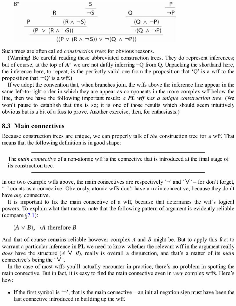
Such trees are often called construction trees for obvious reasons.(Warning! Be careful reading these abbreviated construction trees. They do represent inferences;

but of course, at the top of A″ we are not daftly inferring ¬Q from Q. Unpacking the shorthand here,the inference here, to repeat, is the perfectly valid one from the proposition that ‘Q’ is a wff to theproposition that ‘¬Q’ is a wff.)

If we adopt the convention that, when branches join, the wffs above the inference line appear in thesame left-to-right order in which they are appear as components in the more complex wff below theline, then we have the following important result: a PL wff has a unique construction tree. (Wewon’t pause to establish that this is so; it is one of those results which should seem intuitivelyobvious but is a bit of a fuss to prove. Another exercise, then, for enthusiasts.)

8.3 Main connectivesBecause construction trees are unique, we can properly talk of the construction tree for a wff. Thatmeans that the following definition is in good shape:

The main connective of a non-atomic wff is the connective that is introduced at the final stage ofits construction tree.

In our two example wffs above, the main connectives are respectively ‘¬’ and ‘∨’ – for don’t forget,‘¬’ counts as a connective! Obviously, atomic wffs don’t have a main connective, because they don’thave any connective.

It is important to fix the main connective of a wff, because that determines the wff’s logicalpowers. To explain what that means, note that the following pattern of argument is evidently reliable(compare 7.1):

And that of course remains reliable however complex A and B might be. But to apply this fact towarrant a particular inference in PL we need to know whether the relevant wff in the argument reallydoes have the structure (A ∨ B), really is overall a disjunction, and that’s a matter of its mainconnective’s being the ‘∨’.

In the case of most wffs you’ll actually encounter in practice, there’s no problem in spotting themain connective. But in fact, it is easy to find the main connective even in very complex wffs. Here’show:

If the first symbol is ‘¬’, that is the main connective – an initial negation sign must have been thelast connective introduced in building up the wff.

Otherwise a wff must have the form (A ∧ B) or (A ∨ B), where A and B are themselves wffs.Now, it is a trivial consequence of our rules that any wff A has to have the same number of left-hand and right-hand brackets (the number may be zero, of course!). So, to the left of the mainconnective, there is altogether one more left-hand than right-hand bracket (namely the openingone before the wff A). So, count from the left, find the first ‘∧’ or ‘∨’ which is preceded byexactly one more left-hand than right-hand bracket, and that has to be the main connective.

For an example, take the long wff

Since this doesn’t start with ‘¬’ we apply the second rule; and a simple bracket-count then shows thatthe main connective is the third ‘∨’.

This trick for finding main connectives also gives us a trick for growing construction trees from thebottom up. Start with the given wff. Find the main connective. If it is ‘¬’, write the wff again the nextline up, without its initial negation sign. If it is ‘∧’ or ‘∨’, so the wff has the form (A ∧ B) or (A ∨B), split the tree and write A (the part before the main connective, minus the opening bracket) on theleft branch, and B (the part after the main connective, minus the closing bracket) on the right branch.Repeat the process on the new wffs at the top of the branches, and keep on going until we get toatomic wffs which cannot be further disassembled. (Exercise: apply this to the two wffs in 8.2.)

We can apply this process, in fact, to any string of symbols, wff or otherwise. If all goes well, andwe end up with a completed construction tree with atoms at the tips of the branches, that shows thestring is indeed a wff. If the process breaks down, and we get garbage appearing on the tree where awff should be, then we know that the original string isn’t a wff.

Here’s a couple of quick examples. First, take the long string

Applying the rules for disassembling this into a construction tree, the counting trick yields

The left-hand side is unproblematic. Tackling the right-hand side, we next strip off the negation sign,and then apply the counting trick to get

And now we are obviously in trouble on the right-most branch: we are not going to be able tocomplete a well-formed tree, so the original string we started from cannot be a wff.

Suppose we’d started instead with the following horrendous string:

(Don’t panic, you aren’t really going to encounter this sort of monstrosity in practice: we’re justmaking the point that our technique works irrespective of complexity!) The counting trick tells us tofirst split the string like this:

The rules for bracket-counting and wff-splitting applied on the left, and for negation-stripping appliedon the right, tell us to continue the tree upwards thus:

Another cycle of bracket-counting and negation-stripping and we can go another level up the tree, asfollows:

By this stage it is clear that the tree is going to finish satisfactorily with atoms at the tip of everybranch (complete the tree to that show this claim is true). So the original horrendous string is agenuine wff.

8.4 Subformulae and scopeHere are two more useful syntactic notions which again are neatly introduced using the idea of aconstruction tree:

A wff S is a subformula of a wff A if S appears anywhere on the construction tree for A.The scope of a connective in A is the wff on A’s construction tree where the connective isintroduced.

So, a subformula is a string of symbols occurring within a wff which could equally stand alone as awff in its own right.

Returning to example B above, in the wff

the strings ‘P’, ‘¬P’, ‘(Q ∧ ¬P)’ and ‘¬(Q ∧ ¬P)’ are sample subformulae, and the string ‘¬S)) ∨

¬(Q’ isn’t.Note that our definition allows a wff A trivially to count as a subformula of itself, since it appears

on its own construction tree. The subformulae of A which are shorter than A itself can be called theproper subformulae of A.

Our other definition sharpens up the intuitive idea of scope. By our definition, the scope of the first‘∨’ in our sample wff B is ‘(P ∨ (R ∧ ¬S))’, the scope of the second ‘∨’ is the whole wff, and thescope of the second negation is ‘¬(Q ∧ ¬P)’. A wff, or the occurrence of another connective, is then‘in the scope of’ a given connective in the intuitive sense if it is literally in, i.e. is part of, the scopeas we’ve just technically defined it.

For example, compare the wffs ‘(P ∨ (Q ∧ R))’ and ‘((P ∨ Q) ∧ R)’. Intuitively ‘∧’ is in thescope of ‘∨’ in the first of these, and vice versa in the second. And that tallies with our definition.

Again, note that a connective counts as being in its own scope by our definition: but that’s aharmless wrinkle.

8.5 Bracketing stylesSo much, then, for the official story. Now a quick suggestion about how to make life easier – or atleast, how to make long wffs more readable: mark up pairs of brackets which belong together, toreveal more clearly how the wff is constructed. You can do this in handwriting by using differentsized brackets, or different coloured inks, to signal matching pairs. Here, in this book, we can makeuse of the different available styles for printing brackets. So, for example, take again the wff:

Then, if we bend some of the matching brackets into curly ones ‘{’, ‘}’ and straighten other pairs intosquare ones ‘[’, ‘]’, we get

and the string instantly looks rather more readable (and much more obviously a wff). But we will usethis dodge quite sparingly in what follows, since it is good to get used to reading less complex wffswithout this assistance.

8.6 A final brief remark on symbolismLanguages like PL have been studied and used for a century. In that time, a fair variety of symbolismhas been used. But things have settled down, and the symbolism used in this book is pretty much thestandard one. The only divergences between modern books you are likely to see are these:

some authors use ‘&’ rather than ‘∧’;some authors use ‘∼’ rather than ‘¬’;authors differ in which letters count as atoms, and some provide an unending list of atoms byusing numerical subscripts (thus, ‘P0’, ‘P1’, ‘P2’, …).

In addition, some allow a few special conventions for leaving out brackets in such a way that noambiguities will arise (e.g. you are allowed to omit outermost brackets). None of these variations

should cause you any problems if you encounter them elsewhere.You will find, however, that many books from the outset add to PL a fourth connective ‘⊃’ (or

‘→’). It will become clear soon enough why we aren’t following suit: this additional connective willget introduced in due course, at a more appropriate place (Chapter 14).

8.7 SummaryWe have described the official syntax of PL, which first defines the class of atomic wffs, andthen gives rules for constructing legitimate complex wffs out of simpler ones. The constructionalhistory of a wff can be set out as a unique construction tree.The main connective of a (non-atomic) wff is the final connective added to its construction tree.There are simple rules for finding the main connective of even very complex wffs, and hencesimple rules for ‘disassembling’ a complex string and recovering its construction tree, if it hasone.A subformula of a wff is a substring that would make a stand-alone wff. The scope of aconnective is the subformula where it is introduced in the construction tree.

Exercises 8A Show the following expressions are wffs by producing construction trees for them. Which is the

main connective of each wff? Also, list all the subformulae of the last two examples.

1. ((P ∨ P) ∧ R)2. (¬(R ∧ S) ∨ ¬Q)3. ¬¬((P ∧ Q) ∨ (¬P ∨ ¬Q))4. ((((P ∨ P) ∧ R) ∧ Q) ∨ (¬(R ∧ S) ∨ ¬Q))5. (¬(¬(P ∧ Q) ∧ ¬(P ∧ R))∨¬(P ∧ (Q ∨ R)))6. (¬((R ∨ ¬ Q) ∧ ¬S) ∧ (¬(¬P ∧ Q) ∧ S))

What is the scope of each connective in the wffs (3) and (4)? What wffs are in the scope of each‘∧’ in (5) and (6)?

B Which of the following expressions are wffs of PL?

1. ((P ∨ Q) ∧ ¬R))2. ((P ∨ (Q ∧ ¬R) ∨ ((Q ∧ ¬R) ∨ P))3. ¬(¬P ∨ (Q ∧ (R ∨ ¬P))4. ((P ∧ (Q ∨R)) ∧ (Q ∨R))5. (((P ∧ (Q ∧ ¬R)) ∨ ¬¬¬(R ∧ Q)) ∨ (P ∧ R))6. ((P ∧ (Q ∧ ¬R)) ∨ ¬¬¬((R ∧ Q) ∨ (P ∧ R)))7. (¬(P ∨ ¬(Q ∧ R)) ∨ (P ∧ Q ∧ R)8. ¬¬((¬P ∧ (S ∨¬S)) ∧ ((Q ∧ (P ∧ ¬R)) ∨¬S))

Repair the defective expressions by adding/removing the minimum number of brackets needed todo the job. Show the results are indeed wffs by producing construction trees in each case. What isthe main connective in each case?

9

The semantics of PL

Having described the syntax of PL, we now turn to semantics, i.e. to questions of meaning and truth.And while our syntactic story was thoroughly conventional, now there are more options: the stories invarious text books are subtly but importantly different. Introductory clarity requires that we fix on oneapproach and stick to it. Our line follows through the implications of the two-stage strategy forassessing arguments. The proposal, recall, is that we first render a vernacular argument into a well-behaved artificial language; and then we investigate the validity or otherwise of the reformulatedargument. But if the renditions of arguments into PL are still to be arguments, with contentfulpremisses and conclusions, that means that the atoms of PL cannot be left as mere uninterpretedsymbols: they must be given meaning.

9.1 Interpreting atomic wffsWe interpret the wffs of PL, then, in two stages. First, we assign content to the atomic wffs; and thenwe explain how to work out the meanings of molecular wffs, given we know what their atomiccomponents mean.

We have to specify the content of atoms by a bald list that fixes which propositions are expressedby which atoms – as follows, perhaps:

‘P’ means Alun loves Bethan.‘Q’ means Bethan loves Caradoc.‘R’ means Alun has a dog.‘S’ means The dog is in the kennel.‘P′’ means The cat is on the mat.‘Q′’ means ….

But how long should this list be? We want to be able to render arguments on all kinds of topics intoPL and then assess them: does that mean we need a single huge English-to-PL dictionary to enableall those translations?

No. Remember that our central concern is with the way that certain arguments depend for theirvalidity or invalidity on the use of conjunction, disjunction and negation (rather than on the meaning ofthe atoms). So the translation of atoms is a step to be got out of the way as simply as possible, beforerevealing how the propositional connectives are distributed among premisses and conclusions. Wetherefore treat the atoms of PL as available to code different messages on different occasions ofuse. On any particular occasion, we fix on a code-book that tells us how to interpret the atoms weneed. We’ve just described the beginnings of one code-book. We described another in 7.5. And if,for example, we want to express argument A of 7.1 – ‘Either we are out of petrol or the carburettoris blocked; we are not out of petrol; so the carburettor is blocked’ – we can stipulate that on this

occasion:

‘P’ means We are out of petrol.‘Q’ means The carburettor is blocked.

The argument then gets translated

(P ∨ Q), ¬P ∴ Q

(Now you see what the comma, and the familiar symbol ‘∴’ for therefore, are going to be neededfor!) If encoding that argument is our only current concern, then we don’t need to interpret any of themyriad other atoms of PL which are potentially available to code propositions.

Similarly, if we want to express argument B′ of 7.1 – ‘It’s not true that Tony supports the policyand George does too; Tony supports the policy; so George does not support it’ – then we can stipulatethat on this occasion

‘P’ means Tony supports the policy.‘Q’ means George supports the policy.

So the whole argument gets translated

¬(P ∧ Q), P ∴ ¬Q

In summary, then, the plan is to let the interpretation of atoms (enough atoms for the purposes athand) vary between different applications of PL to encode arguments. What stays permanently fixedas the reading of the atoms changes is the interpretation of the connectives.

9.2 Interpreting molecular wffsAs already explained in Chapter 7, the three connectives get the following constant interpretations.

‘∧’ invariably signifies bare conjunction, no more and no less. So a conjunctive wff of the form(A ∧ B) – i.e. a wff whose main connective is ‘∧’ – means just that A holds and B does too.Similarly, the vel sign ‘∨’ invariably signifies bare inclusive disjunction, no more and no less.In other words, a disjunctive wff of the form (A ∨ B) – i.e. a wff whose main connective is ‘∨’– expresses no more than that A holds, or B holds, or both hold.The basic rule for interpreting wffs starting with a negation sign is even simpler: a wff of theform ¬A expresses the contradictory of A, i.e. that proposition which denies exactly what plain Aasserts.

Given the meanings of the atoms in a wff, it is then easy to work out the corresponding meanings ofcomplex wffs (we’ve already implicitly assumed an ability to do this in the translation examples in 7.5). The only problems will be in hitting on reasonably natural vernacular versions thatunambiguously express the relevant message.

For example, suppose we set:

‘P’ means Jack took Jill to the party.‘Q’ means Jack took Jo to the party.

‘R’ means Jack had some real fun.

Then it won’t do to interpret

(P ∨ (Q ∧ R))

as

Either Jack took Jill to the party or he took Jo and he had some real fun,

for that just reintroduces the very kind of ambiguity which the careful bracketing in PL is there toeliminate (see 7.2, point (4)). An English rendition that expresses the correct interpretationunambiguously would be e.g.

Either Jack took Jill to the party or else he both took Jo and also had some real fun.

9.3 ValuationsOn the first set of interpretations above, ‘P’ means Alun loves Bethan. So ‘P’ says something true justso long as Alun really does love Bethan. Likewise, ‘Q’ means Bethan loves Caradoc. So ‘Q’ sayssomething true just so long as Bethan loves Caradoc. And so on. Now, it is up to us under whatconditions ‘P’ and ‘Q’ say something true, for that’s a matter of the meanings we assign. But havingassigned the meanings, and so fixed the conditions which have to hold for the various atomic wffs tobe true, it is up to the world whether the relevant conditions actually obtain. If Alun does love Bethan,then ‘P’ is true; if not, ‘P’ is false. Likewise if Bethan indeed loves Caradoc, then ‘Q’ is true; if not,then ‘Q’ is false. In this way, our readings of ‘P’, ‘Q’ etc. combine with the facts about Welsh life todetermine a truth-valuation of those interpreted atomic wffs, i.e. an assignment of a truth-value, oneof true or false, to each of them.

But you might ask: does an interpretation for ‘P’ combined with the facts always fix a determinatetruth-value for the atomic wff? Here are four sorts of case to think about:

Perhaps ‘P’ still means Alun loves Bethan, but Alun’s feelings are mixed, on the borderline oflove. So maybe it is neither definitely true that he loves Bethan nor definitely false.Perhaps you are told ‘P’ means Mr Brixintingle loves Bethan. But the name ‘Mr Brixintingle’has just been made up on the spur of the moment and denotes no one. We might be inclined to saythat in this case ‘P’ doesn’t express a complete proposition – there is, so to speak, a gap in it –and hence ‘P’ doesn’t get to the starting line for being assessed for truth or falsehood. Arguably,it is neither true nor false.Perhaps ‘P’ is interpreted as one of those paradoxical claims which says of itself that it is false.So if ‘P’ is false, it is true; and if it is true it is false. Contradiction! What should we say aboutsuch so-called ‘liar sentences’? Perhaps here too we have a case in which ‘P’ is neither true norfalse.Here’s a more sophisticated worry. It can be tempting to think of the truth of some mathematicalpropositions as consisting in their provability, and their falsehood as consisting in theirrefutability. Or at least that view can be tempting if you are puzzled by the alternative idea thatmathematical propositions are made true by how things are in a mysterious Platonic realminhabited by abstract mathematical entities. But then, on the truth-as-provability view, if ‘P’ is

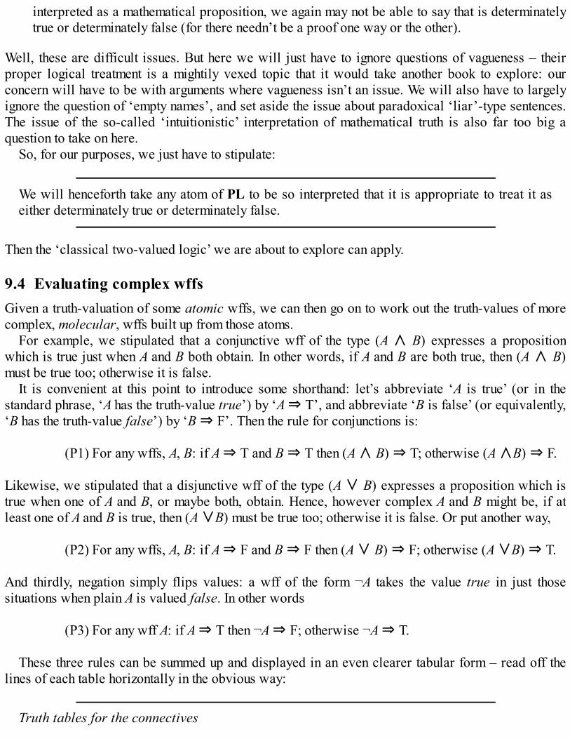
interpreted as a mathematical proposition, we again may not be able to say that is determinatelytrue or determinately false (for there needn’t be a proof one way or the other).

Well, these are difficult issues. But here we will just have to ignore questions of vagueness – theirproper logical treatment is a mightily vexed topic that it would take another book to explore: ourconcern will have to be with arguments where vagueness isn’t an issue. We will also have to largelyignore the question of ‘empty names’, and set aside the issue about paradoxical ‘liar’-type sentences.The issue of the so-called ‘intuitionistic’ interpretation of mathematical truth is also far too big aquestion to take on here.

So, for our purposes, we just have to stipulate:

We will henceforth take any atom of PL to be so interpreted that it is appropriate to treat it aseither determinately true or determinately false.

Then the ‘classical two-valued logic’ we are about to explore can apply.

9.4 Evaluating complex wffsGiven a truth-valuation of some atomic wffs, we can then go on to work out the truth-values of morecomplex, molecular, wffs built up from those atoms.

For example, we stipulated that a conjunctive wff of the type (A ∧ B) expresses a propositionwhich is true just when A and B both obtain. In other words, if A and B are both true, then (A ∧ B)must be true too; otherwise it is false.

It is convenient at this point to introduce some shorthand: let’s abbreviate ‘A is true’ (or in thestandard phrase, ‘A has the truth-value true’) by ‘A ⇒ T’, and abbreviate ‘B is false’ (or equivalently,‘B has the truth-value false’) by ‘B ⇒ F’. Then the rule for conjunctions is:

(P1) For any wffs, A, B: if A ⇒ T and B ⇒ T then (A ∧ B) ⇒ T; otherwise (A ∧B) ⇒ F.

Likewise, we stipulated that a disjunctive wff of the type (A ∨ B) expresses a proposition which istrue when one of A and B, or maybe both, obtain. Hence, however complex A and B might be, if atleast one of A and B is true, then (A ∨B) must be true too; otherwise it is false. Or put another way,

(P2) For any wffs, A, B: if A ⇒ F and B ⇒ F then (A ∨ B) ⇒ F; otherwise (A ∨B) ⇒ T.

And thirdly, negation simply flips values: a wff of the form ¬A takes the value true in just thosesituations when plain A is valued false. In other words

(P3) For any wff A: if A ⇒ T then ¬A ⇒ F; otherwise ¬A ⇒ T.

These three rules can be summed up and displayed in an even clearer tabular form – read off thelines of each table horizontally in the obvious way:

Truth tables for the connectives

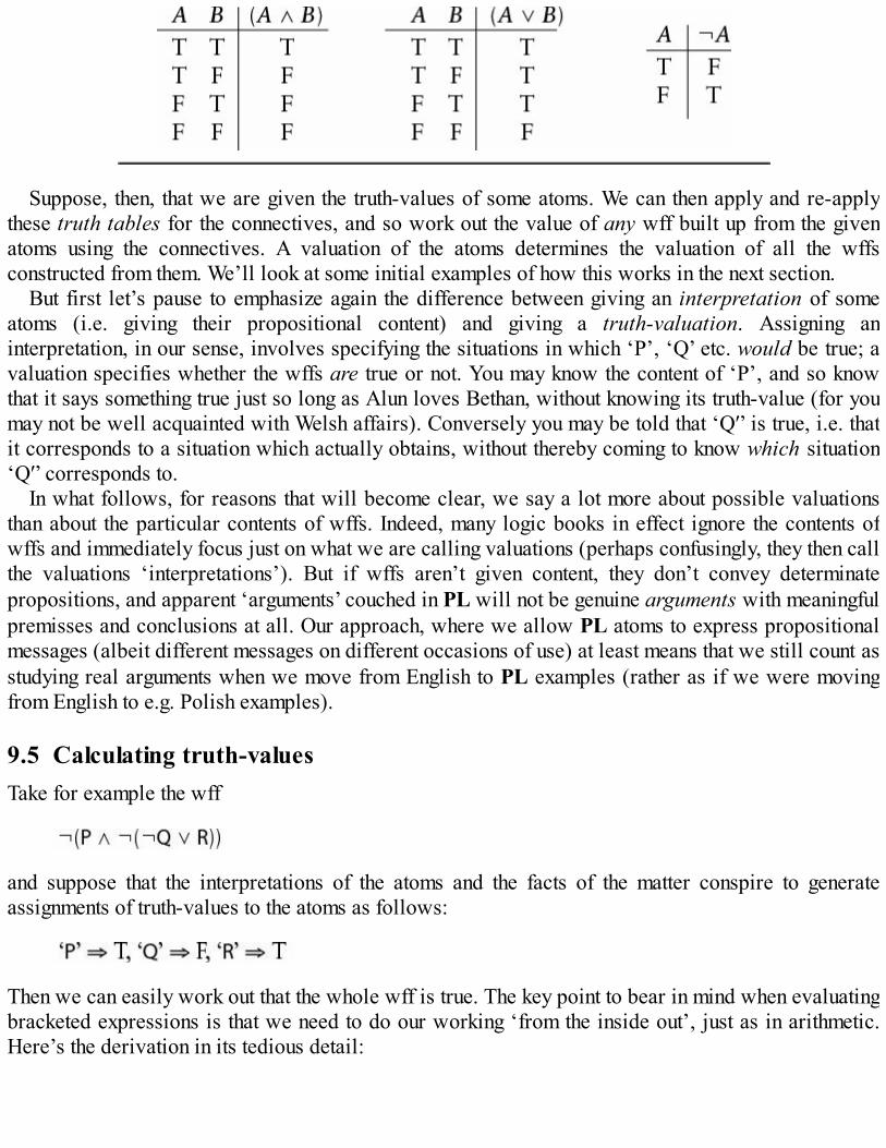
Suppose, then, that we are given the truth-values of some atoms. We can then apply and re-applythese truth tables for the connectives, and so work out the value of any wff built up from the givenatoms using the connectives. A valuation of the atoms determines the valuation of all the wffsconstructed from them. We’ll look at some initial examples of how this works in the next section.

But first let’s pause to emphasize again the difference between giving an interpretation of someatoms (i.e. giving their propositional content) and giving a truth-valuation. Assigning aninterpretation, in our sense, involves specifying the situations in which ‘P’, ‘Q’ etc. would be true; avaluation specifies whether the wffs are true or not. You may know the content of ‘P’, and so knowthat it says something true just so long as Alun loves Bethan, without knowing its truth-value (for youmay not be well acquainted with Welsh affairs). Conversely you may be told that ‘Q′’ is true, i.e. thatit corresponds to a situation which actually obtains, without thereby coming to know which situation‘Q′’ corresponds to.

In what follows, for reasons that will become clear, we say a lot more about possible valuationsthan about the particular contents of wffs. Indeed, many logic books in effect ignore the contents ofwffs and immediately focus just on what we are calling valuations (perhaps confusingly, they then callthe valuations ‘interpretations’). But if wffs aren’t given content, they don’t convey determinatepropositions, and apparent ‘arguments’ couched in PL will not be genuine arguments with meaningfulpremisses and conclusions at all. Our approach, where we allow PL atoms to express propositionalmessages (albeit different messages on different occasions of use) at least means that we still count asstudying real arguments when we move from English to PL examples (rather as if we were movingfrom English to e.g. Polish examples).

9.5 Calculating truth-valuesTake for example the wff

and suppose that the interpretations of the atoms and the facts of the matter conspire to generateassignments of truth-values to the atoms as follows:

Then we can easily work out that the whole wff is true. The key point to bear in mind when evaluatingbracketed expressions is that we need to do our working ‘from the inside out’, just as in arithmetic.Here’s the derivation in its tedious detail:

It is perhaps more perspicuous, though, to lay out the reasoning in a tree form:

Note the direct parallelism between these derivations (in linear and tree form) and the correspondingderivations A and A′ in 8.2 which showed that the wff in question is genuinely well-formed. This isno accident! We have expressly designed PL so that the syntactic structure of a wff, the way that thesymbols are put together into coherent strings, is a perfect guide to its semantic structure and the waythe truth-value of the whole depends on the truth-values of the atoms.

Here’s another example. Take the wff

and suppose ‘P’ ⇒ F, ‘Q’ ⇒ F, ‘R’ ⇒ T, ‘S’ ⇒ F. Then we have (in linear, step by step, detail)

Or putting the same derivation in tree form

Again, notice the exact parallelism with B and B′ in 8.2 above, where we showed that the wff inquestion is indeed a wff.

9.6 Three points about valuations(1) Note that we can do these calculations of the truth-values of complex wffs even when we’veforgotten what their constituent atoms are supposed to mean. That’s because the truth-values of wffsin PL depend only on the truth-values of their parts, and not on the interpretation of those parts.More on this very important point in Chapter 11.

(2) The fact that we evaluate a wff by in effect working down its construction tree means that thevalues of atoms which aren’t on the construction tree can’t matter for the value of the final wff. Inother words, the truth-value of a wff depends only on the assignment of values to the atoms it actuallycontains.

(3) A valuation of the atoms in a wff determines the value of that wff uniquely. That’s because acomplex wff has a unique construction tree; and once values are assigned to the atoms at the tips ofthe branches, the values of the increasingly complex subformulae encountered as you work down thetree are uniquely fixed at each stage by applying the truth-table for the connective introduced at thatstage.

Suppose we hadn’t adopted our strict policy requiring brackets to be used with the (two-place)connectives. Suppose, in other words, that we allowed expressions like ‘P ∨ Q ∧ R’ to count aswell formed. Then this expression would be structurally ambiguous in the sense that it wouldn’thave a unique construction tree. It could built up in either of the following ways:

Imagine that ‘P’ ⇒ T, ‘Q’ ⇒ T, ‘R’ ⇒ F. The wff would then evaluate in both these ways:

Here the final valuations differ because, on the left, the wff is being seen as con-joining a truth and afalsehood (‘∧’ has wider scope than ‘∨’), and on the right as disjoining a different truth andfalsehood (‘∨’ has wider scope). The syntactic structural ambiguity leads to a semantic ambiguity:

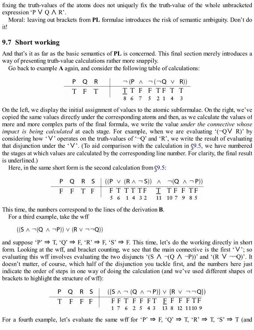
fixing the truth-values of the atoms does not uniquely fix the truth-value of the whole unbracketedexpression ‘P ∨ Q ∧ R’.

Moral: leaving out brackets from PL formulae introduces the risk of semantic ambiguity. Don’t doit!

9.7 Short workingAnd that’s it as far as the basic semantics of PL is concerned. This final section merely introduces away of presenting truth-value calculations rather more snappily.

Go back to example A again, and consider the following table of calculations:

On the left, we display the initial assignment of values to the atomic subformulae. On the right, we’vecopied the same values directly under the corresponding atoms and then, as we calculate the values ofmore and more complex parts of the final formula, we write the value under the connective whoseimpact is being calculated at each stage. For example, when we are evaluating ‘(¬Q∨ R)’ byconsidering how ‘∨’ operates on the truth-values of ‘¬Q’ and ‘R’, we write the result of evaluatingthat disjunction under the ‘∨’. (To aid comparison with the calculation in 9.5, we have numberedthe stages at which values are calculated by the corresponding line number. For clarity, the final resultis underlined.)

Here, in the same short form is the second calculation from 9.5:

This time, the numbers correspond to the lines of the derivation B.For a third example, take the wff

and suppose ‘P’ ⇒ T, ‘Q’ ⇒ F, ‘R’ ⇒ F, ‘S’ ⇒ F. This time, let’s do the working directly in shortform. Looking at the wff, and bracket counting, we see that the main connective is the first ‘∨’; soevaluating this wff involves evaluating the two disjuncts ‘(S ∧ ¬(Q ∧ ¬P))’ and ‘(R ∨ ¬¬Q)’. Itdoesn’t matter, of course, which half of the disjunction you tackle first, and the numbers here justindicate the order of steps in one way of doing the calculation (and we’ve used different shapes ofbrackets to highlight the structure of wff):

For a fourth example, let’s evaluate the same wff for ‘P’ ⇒ F, ‘Q’ ⇒ T, ‘R’ ⇒ T, ‘S’ ⇒ T (and

henceforth let’s not repeat the values of atoms on the right; and we’ll just number off the remainingsteps of the calculation):

Finally, let’s take the same valuation of atoms but this time evaluate the new displayed wff (again,we’ve not repeated the values of the atoms on the right):

Once more, we work from the inside outwards, evaluating the two subformulae in curly brackets, ‘{P∧ (¬S ∨ Q)}’ (step 3), and ‘{¬R ∧ ¬P}’ (step 6) which immediately yields the value of ‘¬{¬R ∧¬P}’ (step 7). That gives us the value of the square-bracketed conjunction (step 8), and so the value ofthe whole wff.

We will introduce some more ways of cutting down working in Chapter 11: but we’ve explainedenough to enable you to tackle some first examples. Of course, you don’t actually need to write downthe step numbers: that’s inessential commentary. Practice quickly makes perfect.

9.8 SummaryAtomic wffs in PL get interpreted, on a particular occasion of use, by being directly assignedmeanings (we do this for as many atoms as we need for the purposes at hand). The connectivesget meanings – expressing bare conjunction, inclusive disjunction, and strict negation – whichremain constant across different uses of PL.The factual meaning of an atom fixes its ‘truth-conditions’ (i.e. tells us which situation has toobtain for the atom to be true). The factual meaning and the state of the world combine to fix thetruth-value of (interpreted) atoms. Or at least, they do so given that we are setting aside cases ofvagueness, paradoxical sentences, etc.The standard interpretation of the connectives means that fixing the truth or falsity of each of thewffs A and B will also fix the truth or falsity of the whole conjunction (A ∧ B), the disjunction(A ∨ B), and the negation ¬A.This means that a valuation of the atoms in a wff of PL (i.e. an assignment of the value true orfalse to each of the relevant atoms) will in fact determine a valuation for the whole wff,however complex it is; and this valuation will be unique because of the uniqueness of itsconstructional history.

Exercises 9A Suppose ‘P’ means Plato is a great philosopher; ‘Q’ means Quine is a great philosopher; ‘R’ means

Russell is a great philosopher. Translate the following sentences into PL.

1. Either Quine is a great philosopher or Russell is.2. Neither Plato nor Quine is a great philosopher.

3. Plato, Russell and Quine are great philosophers.4. Not both Quine and Russell are great philosophers.5. Quine is a great philosopher and Russell isn’t.6. Either Quine and Russell are great philosophers, or Plato is.7. It isn’t the case the Quine is and Russell isn’t a great philosopher.

B Suppose ‘P’ means Fred is a fool; ‘Q’ means Fred knows some logic; ‘R’ means Fred is a rocketscientist. Translate the following sentences into PL as best you can. (What do you think is lost inthe translations, given that PL only has the ‘colourless’ connectives ‘∧’, ‘∨’ and ‘¬’?)

1. Fred is a rocket scientist, but he knows no logic.2. Fred’s a fool, even though he knows some logic.3. Although Fred’s a rocket scientist, he’s a fool and even knows no logic.4. Fred’s a fool, yet he’s a rocket scientist who knows some logic.5. Fred is not a rocket scientist who knows some logic.6. Fred is a fool despite the fact that he knows some logic.7. Fred knows some logic unless he is a fool.

C Confirm that all the following strings are wffs by producing construction trees. Suppose that ‘P’and ‘R’ are both true and ‘Q’ false. Evaluate the wffs by working down the trees. Then do theworking again in the short form.

1. ¬(P ∧ R)2. ¬¬¬¬(Q ∨ ¬R)3. (¬(P ∨ ¬R) ∧ Q)4. ((R ∨ ¬Q) ∧ (Q ∨ P))5. ¬(P ∨ ((Q ∧ ¬P) ∨ R))6. ¬(¬P ∨ ¬(Q ∧ ¬R))7. (¬(P ∧ ¬Q) ∧ ¬¬R)8. (((P ∨ ¬Q) ∧ (Q ∨ R)) ∨¬¬(Q ∨ ¬R))9. (¬(¬P ∨ ¬(Q ∧ ¬R)) ∨¬¬(Q ∨ ¬P))

10. ¬((¬(P ∧ ¬Q) ∧ ¬¬R) ∧ ¬(¬(P ∨ ¬R) ∧ Q))

10

‘A’s and ‘B’s, ‘P’s and ‘Q’s

Before putting PL to use in the following chapters, we should pause to make it absolutely clear howthe ‘A’s and ‘B’s, the ‘P’s and ‘Q’s, are being used, and why it is very important to differentiatebetween them. We should also explain the rules governing the use of quotation marks. By all means,skip this chapter for the moment if you are impatient to get to see our work on PL being put to use: butreturn later, because it is important to get clear on these points.

10.1 Styles of variable: our conventionsWe have been using two styles of symbols, both of which may sensibly be called ‘propositionalvariables’ – namely, italicized letters from early in the alphabet, and roman letters (from a differentfont) from much later in the alphabet. Why two styles? What’s the difference?

‘A’, ‘B’, etc. are handy augmentations of English: they are devices which we are employing inorder to help us speak snappily about patterns of inference, forms of propositions, etc. Forexample, in 7.1, we used them to enable us to talk briskly and clearly, in a slightly expandedEnglish, about patterns of argument involving conjunction and disjunction and couched inEnglish. In 9.4, we used the same variables in order to talk equally briskly and clearly – still inthe same augmented English – about wffs in PL.

As we noted before, such variables, used in presenting patterns in sentences and arguments,are often called schematic variables (the Concise Oxford Dictionary’s entry for ‘schematic’includes ‘representing objects by symbols’). Their use is always dispensable. At the expense ofsome long-windedness, we could always use plain unadorned English prose instead. Schematicvariables do the work that could instead be done by expressions like ‘a first proposition’, or ‘thesecond wff’ and more cumbersome variants. And hence, like those ordinary-language devices,these variables are used to talk about propositions or wffs but do not themselves expresspropositions.On the other hand, ‘P’, ‘Q’, etc. do not belong to English (augmented or otherwise) but insteadare sentences of a new artificial language, PL. And unlike the schematic variables, these newsymbols do themselves potentially express propositions; they encode whole messages, as itmight be about Alun’s loving Bethan, or George’s supporting the policy, or whatever.

We noted that, on different occasions when we translate into PL, we may use ‘P’, ‘Q’, etc. toexpress different messages. We can choose different code-books for associating PL atoms withspecific messages, depending on circumstances (what stays fixed from case to case is themeaning of the connectives). In this sense, the atomic letters can reasonably be thought of as akind of ‘variable’, meaning that the atoms are open to various interpretations. But the contrastremains: schematic variables like ‘A’, ‘B’, etc. are used in augmented English to talk about

propositions and arguments; ‘P’, ‘Q’ etc. belong to PL and express propositions on all kinds ofsubject matter, depending on the code-book or interpretation-manual currently in force.

Sometimes the point is put like this. ‘P’, ‘Q’ and so on belong to the language PL which is – for themoment – the object of our logical studies. In short, these symbols belong to the object-language.And we must in general distinguish the language which is the object of investigation from themetalanguage, i.e. the language in which we conduct the investigation and discuss what is going on inthe object-language. In this book, the metalanguage is English augmented with variables like ‘A’, ‘B’,etc. (so those schematic variables are often also called metalinguistic variables). In a Spanishtranslation of this book, the object language will again be PL, but then the metalanguage will beSpanish. (Of course, we may often want to discuss facts about the logical features of Englishsentences in English – and then the metalanguage subsumes the object language: but in the generalcase they are distinct.)

In this book we adopt the convention that the elements of formal languages like PL will alwaysbe printed in sans-serif type, like ‘P’ and ‘Q’. Symbols printed in serif italics, like ‘A’, ‘n’,‘F’, etc., are always augmentations of our English metalanguage.

An alternative convention widely adopted in other books is to use Greek letters as metalinguisticvariables.

10.2 Basic quotation conventionsNow for some quick remarks about our related usage of quotation marks. We start by warming upwith a few general observations.

If we want to mention a certain man, we may use his name – as it might be

Socrates.

But sometimes we want to discuss not the man but his name. There are various ways of picking outthat philosopher’s name, e.g. laboriously

The name consisting of the nineteenth letter of the alphabet, followed by the fifteenth letter,followed by the third letter, ….

Or indirectly, e.g.

The name which is displayed on the fourth line of this section.

Most simply, we can use quotation marks, thus:

‘Socrates’

with the convention that the whole expression including the quotation marks is to be construed asstanding for the word displayed inside the quotes.

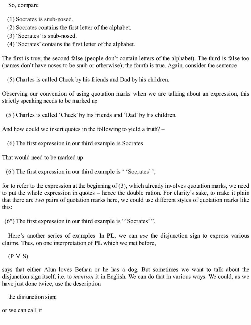
So, compare

(1) Socrates is snub-nosed.(2) Socrates contains the first letter of the alphabet.(3) ‘Socrates’ is snub-nosed.(4) ‘Socrates’ contains the first letter of the alphabet.

The first is true; the second false (people don’t contain letters of the alphabet). The third is false too(names don’t have noses to be snub or otherwise); the fourth is true. Again, consider the sentence

(5) Charles is called Chuck by his friends and Dad by his children.

Observing our convention of using quotation marks when we are talking about an expression, thisstrictly speaking needs to be marked up

(5′) Charles is called ‘Chuck’ by his friends and ‘Dad’ by his children.

And how could we insert quotes in the following to yield a truth? –

(6) The first expression in our third example is Socrates

That would need to be marked up

(6′) The first expression in our third example is ‘ ‘Socrates’ ’,

for to refer to the expression at the beginning of (3), which already involves quotation marks, we needto put the whole expression in quotes – hence the double ration. For clarity’s sake, to make it plainthat there are two pairs of quotation marks here, we could use different styles of quotation marks likethis:

(6″) The first expression in our third example is “‘Socrates’ ”.

Here’s another series of examples. In PL, we can use the disjunction sign to express variousclaims. Thus, on one interpretation of PL which we met before,

(P ∨ S)

says that either Alun loves Bethan or he has a dog. But sometimes we want to talk about thedisjunction sign itself, i.e. to mention it in English. We can do that in various ways. We could, as wehave just done twice, use the description

the disjunction sign;

or we can call it

the vel sign.

The vel sign itself is no part of English, though the expression ‘vel’ is used as part of logician’sEnglish: it is the name they use for the PL connective. We could also use quotation marks again, thus:

‘∨’

And this composite expression is available for use in English to refer to the disjunction sign in PL,as when we say that ‘∨’ is a two-place connective. (Compare: the word

soleil

is no part of English. However we can use the expression

‘soleil’

in an English sentence – as when we say that the French word ‘soleil’ means sun.)Similarly for the atomic letters of PL. With a translation manual in place, we can use them as

sentences of PL (to talk about Welsh affairs, or whatever it might be). But we also want to mentionthe atoms, i.e. talk about them in English, our metalanguage. Again the easiest way of doing that is touse quotation marks to form expressions (augmenting English!) to refer to expressions in PL. Thus wemay write, in English,

(7) The atomic sentences ‘P’ and ‘S’ are constituents of the molecular sentence ‘(P ∨ S)’.

Likewise, we may write, still in English,

(8) ‘P’ takes the value true.

So compare

(9) ‘P’ is a sentence of PL(10) ‘P’ is a sentence of English(11) “‘P’” is an expression which can occur in PL sentences(12) “‘P’” is an expression which can occur in English sentences

The first is true, but the second is false; the third is false too (since PL doesn’t contain quotationnames of anything, only atomic sentences and their molecular compounds). The last, however, is true;for example, (10) provides an instance of an English sentence where the quotation of ‘P’ occurs.

In summary: it is important to grasp both the distinction between object-language and metalanguage‘variables’ (signalled in this book by the use of different fonts), and also the distinction between theuse and mention of expressions (standardly signalled by quotation marks). And because thedistinctions matter and ignoring them can lead to confusion, it is important to fix on officialconventions for marking them clearly.

However, having said that, sometimes we can forgivably relax the conventions when doing so

promotes readability, and there is no danger of confusion – after all, we are in charge, and we don’tneed to be slaves to our own conventions! For example, strictly we should write e.g.

‘P’ takes the value true, ‘Q’ takes the value false.

Or (as we did in the last chapter)

‘P’ ⇒ T, ‘Q’ ⇒ F

But from now on we will typically take ‘⇒’ to come with unwritten quotation marks affixed, andwrite more causally

P ⇒ T, Q ⇒ F

and so forth. That’s a bit tidier, cutting down on a rash of quotation marks. But it must just beremembered these are still metalinguistic claims: the expression ‘⇒ T’ does not belong to PL, but isshorthand added to English.

10.3 A more complex conventionThis section notes a wrinkle, and straightens it out.

In 8.1, we stated the wff-building rule W3 in abbreviated form as

If A and B are wffs, so is (A ∧ B).

The intended reading of this rule would probably have been entirely obvious, even if we hadn’t givena non-abbreviated version of the rule at the same time. But our shorthand version does mix augmentedEnglish (the schematic variables ‘A’ and ‘B’) with expressions from PL (the conjunction sign, ofcourse, but also the two brackets as well). And we can’t untangle things by writing

If A and B are wffs, so is ‘(A ∧ B)’,

for what is inside the quotes here is not a wff of PL (remember, ‘A’ and ‘B’ are not symbols of thatlanguage).

If we want to be really accurate, then we will need to introduce a new brand of quotation marks(‘corner quotes’, often called ‘Quine quotes’ after their inventor). So we write

If A and B are wffs, so is (A ∧ B)

Here, ‘ (A ∧ B) ’ is short for

the result of writing ‘(’ followed by A followed by ‘∧’ followed by B followed by ‘)’.

For example, suppose A is the wff ‘(P ∨ S)’, and B is the wff ‘Q’. Then the conjunction of those twowffs is indeed (A ∧ B) , i.e. it is the result of writing ‘(’ followed by ‘(P ∨ S)’ followed by ‘∧’followed by ‘Q’ followed by ‘)’, which is ‘((P ∨ S) ∧ Q)’, just as we want.

Here’s another sort of case where we can use Quine-quotes. As we’ll note in 12.2,

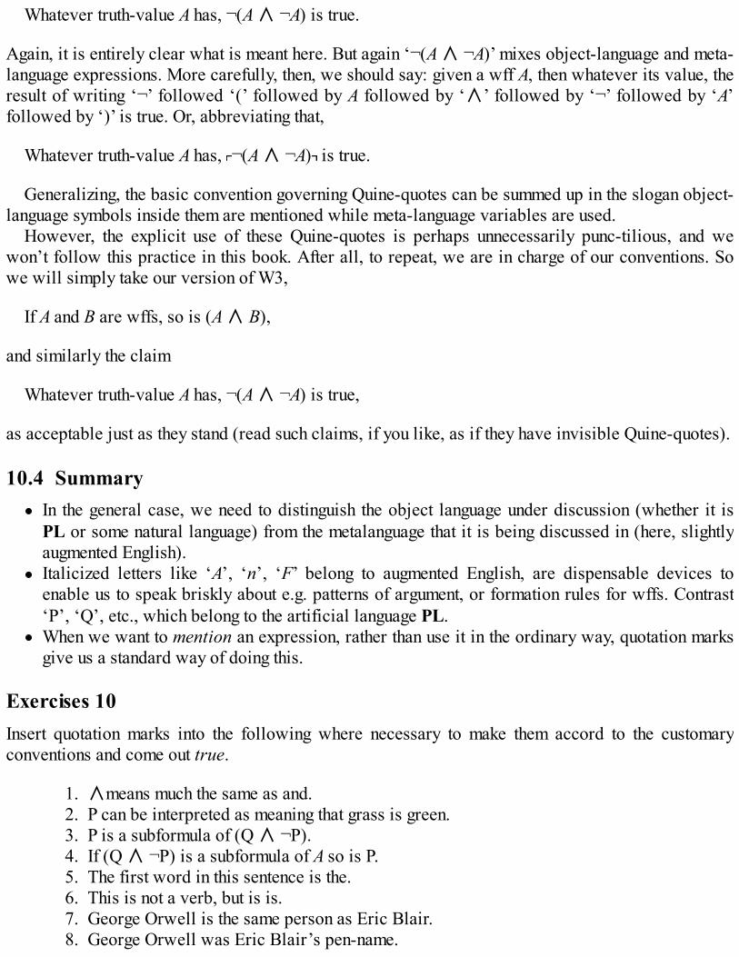
Whatever truth-value A has, ¬(A ∧ ¬A) is true.

Again, it is entirely clear what is meant here. But again ‘¬(A ∧ ¬A)’ mixes object-language and meta-language expressions. More carefully, then, we should say: given a wff A, then whatever its value, theresult of writing ‘¬’ followed ‘(’ followed by A followed by ‘∧’ followed by ‘¬’ followed by ‘A’followed by ‘)’ is true. Or, abbreviating that,

Whatever truth-value A has, ¬(A ∧ ¬A) is true.

Generalizing, the basic convention governing Quine-quotes can be summed up in the slogan object-language symbols inside them are mentioned while meta-language variables are used.

However, the explicit use of these Quine-quotes is perhaps unnecessarily punc-tilious, and wewon’t follow this practice in this book. After all, to repeat, we are in charge of our conventions. Sowe will simply take our version of W3,

If A and B are wffs, so is (A ∧ B),

and similarly the claim

Whatever truth-value A has, ¬(A ∧ ¬A) is true,

as acceptable just as they stand (read such claims, if you like, as if they have invisible Quine-quotes).

10.4 SummaryIn the general case, we need to distinguish the object language under discussion (whether it isPL or some natural language) from the metalanguage that it is being discussed in (here, slightlyaugmented English).Italicized letters like ‘A’, ‘n’, ‘F’ belong to augmented English, are dispensable devices toenable us to speak briskly about e.g. patterns of argument, or formation rules for wffs. Contrast‘P’, ‘Q’, etc., which belong to the artificial language PL.When we want to mention an expression, rather than use it in the ordinary way, quotation marksgive us a standard way of doing this.

Exercises 10Insert quotation marks into the following where necessary to make them accord to the customaryconventions and come out true.

1. ∧means much the same as and.2. P can be interpreted as meaning that grass is green.3. P is a subformula of (Q ∧ ¬P).4. If (Q ∧ ¬P) is a subformula of A so is P.5. The first word in this sentence is the.6. This is not a verb, but is is.7. George Orwell is the same person as Eric Blair.8. George Orwell was Eric Blair’s pen-name.

9. The Evening Star and The Morning Star denote the same planet.10. Sappho is a Greek poet.11. Sappho is the name of a Greek poet.12. If we want to refer not to Sappho but her name, we need to use the expression Sappho.

11

Truth functions

We noted in 9.6 that if we assign truth-values to the atoms in a wff of PL, then this will uniquelydetermine the truth-value of the whole wff. This feature of the language is called truth-functionality:it is the topic of the present chapter.

11.1 Truth-functional vs. other connectivesLet’s start with a definition.

A way of forming a complex sentence out of one or more constituent sentences is truth-functional if fixing the truth-values of the constituent sentences is always enough (whateverthose values are) to determine the truth-value of the whole complex sentence.

Note that this definition applies quite generally, to ordinary-language constructions as well as toconstructions in formal languages like PL.

Some ordinary-language devices do indeed seem to be truth-functional in this sense (e.g. many usesof ‘and’ as a propositional connective). For a contrasting case, consider the two-place connective‘because’. Suppose

(1) The bridge fell down,

and

(2) There was a storm yesterday,

are both true. That plainly doesn’t settle the truth-value of

(3) The bridge fell down because there was a storm yesterday.

The joint truth of (1) and (2) is compatible with the truth of (3); it’s equally compatible with thefalsehood of (3). Hence fixing the truth-values of the constituent sentences (1) and (2) isn’t alwaysenough to determine the truth-value of the complex sentence (3). Hence ‘because’ is not truth-functional.

Of course, if A is false or B is false, A because B will be false too. For example, (3) must be falseif the bridge in fact didn’t fall down, or if there wasn’t a storm. But for full truth-functionality, as wedefined it, the truth-values of the constituents must always determine the truth-value of the whole,

whatever the values are. As we’ve just seen, that doesn’t hold for ‘because’.The same goes for many other constructions which embed sentences inside more complex ones. For

example, consider:

It is widely believed that A.It is more likely that A than that B.It is necessarily true that A.

In each case, merely settling the truth-values of A and B won’t settle (or at least, won’t invariablysettle) the truth-value of the whole sentence.

It is worth pausing on the last of these. Compare, e.g.

(4) The President of the USA in 2008 was male.(5) If someone is a brother, then he is male.

Both are true. But the first might not have been so: we can readily imagine an alternative historicalscenario which leads to a woman President occupying the White House in 2008. The second,however, is necessarily true: just in virtue of what it is to be a brother (i.e. to be a male with at leastone sibling), we cannot coherently conceive of anyone who is a brother but not male. So despite thefact that (4) and (5) both take the truth-value true, the following differ in truth-value:

(4′) It is necessarily true that the President of the USA in 2008 was male.(5′) It is necessarily true that if someone is a brother, then he is male.

In short, the truth-value of ‘It is necessarily true that A’ is sensitive to the particular content of theembedded proposition A, and not just to A’s truth-value.

However, every wff of pure PL (no matter its degree of complexity) is a truth-functionalcombination of the atoms it contains. That is to say, fixing the truth-values of atoms always uniquelyfixes the truth-value of the whole wff. As we noted in 9.6, the basic valuation rules for the threeconnectives in PL plus our fussiness about bracketing secures this result.

11.2 A very brief word about ‘functions’Why is the term ‘truth-functional’ apt?

You will be familiar with the idea of an arithmetical function which takes as input one or morenumbers, and spits out a unique value. For example, ‘the square of x’ denotes a function mapping agiven number x to a definite value, the result of multiplying x by itself. ‘x + y’ denotes anotherfunction, this time mapping two numbers to their sum.

We can generalize this idea of a function to cover any sort of mapping that relates one or moreobjects to a single determinate ‘value’. For example, ‘the biological mother of x’ denotes a functionmapping people to other people. ‘The age in years of x’ denotes another function defined over people,this time correlating each person with a number. ‘The distance in metres between a and b’ maps twospatially located objects to another number.

By contrast, ‘teacher of x’, ‘house belonging to x’, and ‘daughter of x’ don’t express functions; theydon’t express ways of mapping people to unique ‘values’. Some people have more than one teacher,

more than one house and more than one daughter.Given our general notion of a function, what is expressed by a truth-functional mode of sentence

combination is indeed a truth-function. For by definition, a complex sentence which is truth-functional combination of simpler embedded sentences will always map the truth-values of itsconstituents sentences to a single determinate truth-value for the combination as a whole.

11.3 Full truth-tablesConsider again the wff ‘¬(P ∧ ¬(¬Q ∨ R))’. In 9.5, we specified one particular valuation for itsatoms. Because this is a truth-functional mode of combining the atoms, settling on that valuationsufficed to fix the value of the whole wff. But that was just one possible valuation out of many. Thereare in all eight possible valuations of three atoms. There are two ways we can assign a value to ‘P’,each of these can combine with either value for ‘Q’, and each of these combinations can combinewith either value for ‘R’, and 2 × 2 × 2 = 8.

Running through these eight valuations in turn, we can mechanically compute the truth-value of oursample wff in every case. We can set out the working in a neat tabular form. Putting in absolutely allthe details, we have:

On the left, we systematically display the eight different possible assignments of truth-values to thethree atoms. On the right we record the calculation of the truth-value of the wff using (as before) theconvention that we write the value of each subformula under the connective whose effect is beingcalculated. The supplementary numbers at the foot of the columns indicate the order in which we’veworked out the columns. We’ve first copied across the assignments of values to atoms. Then atsubsequent stages we evaluate subformulae of increasing complexity, until – at the final stage,yielding the underlined values – we get to evaluate the whole wff.

Here’s another example, this time involving four atoms, and so requiring sixteen lines of working:

[¬{(R ∨ ¬Q) ∧ ¬S} ∨ {¬(¬P ∧ Q) ∧ S}]

Note again how the little dodge introduced in 8.5 of using different styles of brackets can promotereadability: the main connective is evidently the second disjunction. And this time, as in the lastexamples in 9.7, let’s not bother repeating the values of the atoms on the right of the table (whichsaves time even if it perhaps slightly increases the risk of error):

Take careful note of the system used in listing the possible assignments of values to a sequence ofatoms. The last atom in the sequence gets alternating Ts and Fs; the previous one gets alternatingblocks of two Ts and two Fs; moving left-wards, we get next alternating blocks of four Ts and four Fs;and so it goes. This system is guaranteed to cover all the possible valuations. Any other systematiclayout will do, of course. But ours is pretty much the standard convention.

Suppose there are n different atoms in the wff A. There will be 2 × 2 × … × 2 (n times) = 2n

different possible valuations of these n atoms. We can then always construct a full truth-table for A,working out the truth-values of all the increasingly large subformulae of A until we reach the overallvalue of A for each possible valuation of the atoms. As n increases, however, the amount of labourrequired will explode exponentially.

11.4 ‘Possible valuations’Before continuing, an important word of clarification here. In the last section, we set out a couple ofcomplete truth-tables without any attention to the interpretations of the atoms in our example wffs.Truth-functionality means precisely that the truth-values of complexes can be settled by attending onlyto the truth-values of their atoms. Yet shouldn’t interpretations come back into the story after all?Suppose that (according to the code-book currently in play) ‘P’ has the content All brothers are male,and therefore expresses a necessary truth. In this case there is no valuation which respects themeaning of ‘P’ yet assigns it the value false. Or again, suppose that ‘P’ has the content Jack ismarried, and ‘Q’ the content Jack is single. In this case there is no valuation which respects themeanings of ‘P’ and ‘Q’ yet gives them the same truth-value.

Return then to our sample wff ‘¬(P ∧ ¬(¬Q ∨ R))’ which contains three atoms. Maybe not alleight different assignments of values to these atoms are genuinely possible ones: won’t that depend onthe interpretations of the atoms? So shouldn’t we take that into account when setting out the truth-table

for an interpreted wff?No. Or at least, not given the wider setting of our interest in PL. For our target in developing this

language is to give an account of the logic of arguments whose relevant logical materials are just theconnectives ‘and’, ‘or’ and ‘not’, i.e. arguments whose validity does not rely on the meaning of theiratomic propositional constituents. Given this target, we can and should temporarily ignore the factsabout the meaning of atoms, and concentrate only on those constraints on the overall assignments oftruth-values to wffs which are due to the meanings of the connectives ‘∧’, ‘∨’ and ‘¬’. Hence, givenour particular target, we should put no restrictions on the valuation of atoms. That means that we willcontinue to treat any assignment of T or F to the atoms ‘P’, ‘Q’, etc., as equally legitimate for ourspecial purposes, whatever the meanings of the atoms. In short, we will continue to allow anyvaluation of atoms.

11.5 Short cutsWith a bit of practice, we can learn to skip much of the laborious detail involved in setting out fulltruth tables. For a start, it quickly becomes easy to do some of the working ‘in our heads’. Supposethe formula to be evaluated is

(¬(P ∧ ¬Q) ∨ (R∨(Q ∧ P))).

This wff is the disjunction of the subformulae ‘¬(P ∧ ¬Q)’ and ‘(R∨(Q ∧ P))’, and it is relativelyeasy to work out the truth values of these disjuncts on a given valuation of the atoms in your head.That gives us the entries under the subformulae in the following table, leaving just the value of wholedisjunction to be worked out at the final step:

We can, however, speed things up even more by leaving out any redundant working. In particular, notethese two obvious truisms:

Once a disjunct has been shown to be true, the whole disjunction must be true (so it is redundantto evaluate the other disjunct).Once a conjunct has been shown to be false, the whole conjunction must be false (so it isredundant to evaluate the other conjunct).

Hence, in our last example, as soon as we have evaluated the first disjunct, we can get to the

following:

So we only need to evaluate the second disjunct on just two lines in order to complete the table.Here’s another example. Suppose we are faced with the wff

(¬{Q ∨ [(S ∧ R) ∨ ¬(R ∨ ¬Q)]} ∧ { P ∧ ¬ S})

Bracket-counting confirms that the main connective is indeed the second ‘∧’. So this is a conjunctionwhose second conjunct ‘{ P ∧ ¬ S}’ is simple to evaluate:

Since the big conjunction must be false whenever its second conjunct is false, that has immediatelysettled the value of the wff on twelve of the sixteen lines. Which leaves just four lines to go. Thesecond and fourth lines are relatively easy too. ‘{Q ∨ ((S ∧ R) ∨ ¬(R ∨ ¬Q))}’ is a disjunction

whose first disjunct is simply ‘Q’. Hence whenever ‘Q’ is true, that curly-bracketed subformula willbe true. So its negation is false. Thus we can quickly fill in two more lines of working:

Very quickly we are left with just two final lines of working to fill out. And then the table is speedilycompleted (do it!).

To be sure, even with these short cuts (which you soon get the hang of using), working out completetruth-tables for complex formulae is a tedious business. Fortunately, when it comes to using truth-tables in earnest, we rarely need to consider other than pretty simple formulae. There’s no need forpanic!

11.6 Truth-functional equivalenceSuppose we evaluate ‘((P ∧ ¬Q) ∨ (¬P ∧ Q))’ and ‘((P ∨ Q) ∧ ¬(P ∧ Q))’ for each possibleassignment of values to ‘P’ and ‘Q’. Suppressing the detailed working, we get

The two wffs thus share the same values on each valuation: the full tables with the working laid out inall its detail will of course be different, but the resulting table of final values for the whole wffs areexactly the same. We will say that wffs like this are (truth-functionally) equivalent. A little morecarefully:

The PL wffs A and B are truth-functionally equivalent just if, on each valuation of all the atomsoccurring in them, A and B take the same value.

Equivalent wffs A and B are true in exactly the same circumstances. That means, for example, that if Acan be inferred to be true on the basis of certain premisses, then so can B. Likewise, if A can be usedas a premiss in drawing a certain logical conclusion, then B could equally well be used for the samepurposes. In short, equivalent wffs have the same logical powers.

So when translating ordinary claims into PL for logical purposes, it cannot matter greatly which oftwo truth-functionally equivalent translations we choose. Suppose then we want to translate ‘EitherJack drank beer or he drank cider’ where the ‘or’ is in this case intended to be exclusive. Using ‘P’for Jack drank beer and ‘Q’ for Jack drank cider, we want a translation which comes out true whenexactly one of ‘P’ and ‘Q’ is true: we have just seen that ‘((P ∧ ¬Q) ∨ (¬P ∧ Q))’ or ‘((P ∨ Q) ∧¬(P ∧ Q))’ will do equally well.

That last point fulfils a much earlier promise to show how to express exclusive disjunction in PL (7.4). We could have introduced a new symbol ‘⊕’ into the language with the stipulation that a wff of

the form (A ⊕ B) is true when exactly one of A and B is true. But we can now see that this would bestrictly speaking redundant; we can capture exclusive disjunction using the three connectives alreadyto hand. More precisely: for any wff we could construct using ‘⊕’ in an extension of PL, there is atruth-functionally equivalent wff already available in original, unaugmented PL.

11.7 Expressive adequacyThat last point generalizes. Take any possible truth-functional combination of atoms (which we mightperhaps express using a new connective added to PL): then we can construct an equivalent wff usingjust the original three connectives of PL. This result is a very important one – for it shows that PL,despite its meagre resources, can express a lot more than you might guess. Its resources are enough tocapture any truth-functional way of combining propositions, and so the language is adequate for thewhole of the logic of truth-functions.

The proof of this result is pretty straightforward, but is interesting enough to be worth setting out ina little detail. (This is our first significant ‘metalogical’ result: i.e., it is a general result about ourformal logical apparatus.)

We start with a trivial notational point and then a definition. First, we are going to be writing downsome expressions which look like the following

(A ∧ B ∧ C){A ∨ B ∨ C ∨ D ∨ E}

when strictly speaking – given our rule that each occurrence of ‘∧’ and ‘∨’ comes with its own setof brackets – we ought to write something like

((A ∧ B) ∧ C)((((A ∨ B) ∨ C) ∨ D) ∨ E)

Still, the particular choice of internal bracketing for long unmixed conjunctions or for long unmixeddisjunctions evidently doesn’t affect the truth-value of the resulting wffs (see Exercise 11D). Soleaving out the bracketing in such cases will for once do no real harm, and will make for readability.

Now for our definition. Take any set of atomic wffs, as it might be {P, Q, S, P′}; a basicconjunction is formed by taking each of the atoms in turn, either naked or negated but not both, andthen (if we start with more than one atom) conjoin-ing the results, yielding e.g.

(P ∧ ¬Q ∧ ¬S ∧ P′)(¬P ∧ ¬Q ∧ S ∧ ¬P′)

(¬P ∧ ¬Q ∧ ¬S ∧ ¬P′)

A basic conjunction is true on one and only one assignment of values to its constituent atoms. In ourexamples, the first wff is true just when P ⇒ T, Q ⇒ F, S ⇒ F, P′ ⇒ T; the second true just when P ⇒F, Q ⇒ F, S ⇒ T, P′ ⇒ F; and the third when P ⇒ F, Q ⇒ F, S ⇒ F, P′ ⇒ F. In an obvious sense,then, a basic conjunction corresponds to a particular valuation of its atoms. (Incidentally, note thatour definition allows a basic conjunction to consist in a single atom, if that’s all we start off from!)

With those preliminaries, here’s the proof we want.

A way of constructing a sentence out of PL atoms is truth-functional if fixing the truth-values ofthe constituent atoms is enough to determine the value of the complex sentence. Hence, we canwrite down a truth-table displaying how the value of the truth-functional construction depends onthe values of its components. So our task is effectively this: to show that for any given truth-table, we can write down a PL wff with exactly that truth-table. Now, there are an unlimitednumber of different modes of truth-functional composition of atoms. But however many atomsare in question, one of three things must happen in the resulting truth-table for the combination:either it has ‘F’s all the way down; or it has ‘T’ on exactly one line; or it has ‘T’ on more thanone line. Take these cases in turn.First case When the truth-function is invariably false, it is easy to write down a PL wff using thesame atoms which is also invariably false. Just conjoin or disjoin some contradictions. If ‘!(P,Q, R, S)’ is defined to be a function of those four atoms which is false on every valuation, thene.g.

((P ∧ ¬P) ∨ (Q ∧ ¬Q) ∨ (R ∧ ¬R) ∨ (S ∧ ¬S))

is, careless bracketing apart, a corresponding wff of PL which involves the same atoms and isalso always false.Second case When the truth-function in question takes the value true on exactly one valuation ofatoms, simply write down the PL basic conjunction that corresponds to that particular valuation,and again we have a wff with the desired truth table. For example, if ‘%(P, Q, R, S)’ is true justwhen P ⇒ F, Q ⇒ T, R ⇒ F, S ⇒ T, then

(¬P∧Q∧¬R∧S)

is a wff with the right truth-table.Third case When the truth-function in question takes the value true on a number of differentvaluations of atoms, then (a) write down the PL basic conjunction corresponding to eachvaluation of atoms which makes the function come out true, and then (b) disjoin the results – i.e.write down a long disjunction, where each disjunct is one of those basic conjunctions. This wffwill come out true when and only when some disjunct is true, i.e. when one of those basicconjunctions is true, i.e. on the lines where the target truth-function is true. So our PL wff has thedesired truth-table. For example, the following table defines a perfectly good truth-function of the three atoms ‘P’,‘Q’ and ‘R’:

This dollar truth-function might not be a terrifically interesting one: still, we might want toexpress it, and we can express it in PL, without having to expand the language. Write down abasic conjunction corresponding to each assignment of values where $(P, Q, R) is true, and thendisjoin them. That yields

{(P ∧ Q ∧ ¬R) ∨ (¬P ∧ Q ∧ R) ∨ (¬P ∧ Q ∧ ¬R) ∨ (¬P ∧ ¬Q ∧ R) ∨ (¬P ∧ ¬Q∧ ¬R)}

This is custom built to have the right truth-table, for it comes out true on each line where one ofthe basic conjunctions is true. By construction, then, it is truth-functionally equivalent to $(P, Q,R). It may not be the simplest way of capturing the truth-function $ in PL – ‘(¬P ∨ (Q ∧ ¬R))’does the job, as you can easily verify – but it is certainly one way.

We can sum all that up as follows in another definition and a result:

A set of connectives is expressively adequate if a language containing just those connectives isrich enough to express all truth-functions of the atomic sentences of the language (i.e. rich enoughto enable us to construct a formula with any given truth-table). We have proved that the standardset of PL connectives {∧, ∨, ¬} is expressively adequate.

11.8 ‘Disjunctive normal form’Just for the record, and because you might come across the idea elsewhere, here’s a corollary of ourresult about expressive adequacy. (But you can skip this!)

Start with some more definitions. Let’s say that a wff is a primitive wff if it is either an atom or anegated atom (sometimes the alternative term ‘a literal’ is used). And let’s say that a wff is a basic*conjunction if it consists of a conjunction of one or more primitives. The big difference between abasic and a basic* conjunction is that the latter allows the same atom to appear both negated and un-negated, i.e. it allows contradictions. So basic conjunctions are basic*, but not always vice versa.(Note again we allow basic* conjunctions with only one ‘con-junct’!) Further, we say that a wff is indisjunctive normal form (DNF) if it consists of one or more disjuncts each of which is a basic*conjunction. (Note that we also allow the limiting case of a single ‘disjunct’; in other words, a basic*conjunction by itself counts as being in DNF.)

In these terms, then, what we have just shown is that any truth-functional combination of atoms

can be expressed by an equivalent wff in DNF. As we saw, in the first type of case in the proof in thelast section, where the combination is always false, we can use a disjunction of basic* conjunctionswhich are contradictions. In the second type of case, where the combination is true on just oneassignment of values to atoms, we use a single basic (and hence basic*) conjunction. And in the thirdtype of case, where the combination is true on more than one assignment of values to atoms, we use adisjunction of two or more basic (and hence again basic*) conjunctions.

Since any PL wff expresses a truth-functional combination of atoms, that shows that any wff istruth-functionally equivalent to one in DNF.

11.9 Other adequate sets of connectives.The key adequacy result is the one proved in the 11.7. But it is worth noting that we can do evenbetter: the set of connectives {∧, ¬} is adequate by itself. For a wff of the form (A ∨ B), which rulesout A and B being both false, is equivalent to the corresponding wff of the form ¬(¬A ∧ ¬B). So,given a wff involving occurrences of ‘∧’, ‘∨’ and ‘¬’, we can always construct an equivalent wffinvolving just ‘∧’ and ‘¬’: replace the disjunctions with equivalent negation-conjunctioncombinations.

We can likewise show that the set of connectives {∨, ¬} is adequate: simply note the result that (A∧ B) is equivalent to ¬(¬A ∨ ¬B), and then the argument goes similarly.

However, it is easily seen that {∧, ∨} is not expressively adequate. Looking at the truth-tablesfor those connectives, we see that any wff built using just conjunction and disjunction must be truewhen its atoms are all true. So using conjunction and disjunction we can never get anything equivalentto a wff like ‘¬P’ or ‘(¬P ∨ ¬Q)’ which happens to be false when its atoms are true. Hence there aretruth-functions which can’t be expressed using conjunction and disjunction alone.

The result that any truth-function can be expressed using just a pair of connectives is surely enoughto satisfy any sensible taste for economy. But it is mildly diverting to show in conclusion there are infact single connectives which, just by themselves, are expressively adequate.

Given that {∧, ¬} is expressively adequate, it is enough to find a single connective in terms ofwhich both those connectives can in turn be defined. Clearly it must be at last a two-place connective,and one candidate is the following:

An expression of the form (A ↓ B) says neither A nor B, i.e. that the connected expressions are bothfalse: so we have

¬A is equivalent to (A ↓ A), since that says that A and itself are both false. (A ∧ B), which saysthat neither ¬A nor ¬B, is equivalent to (¬A ↓ ¬B) and so can be expressed by ((A ↓ A) ↓ (B ↓ B)).

Thus any PL wff built up by conjunction and negation can in principle be laboriously rewritten usingjust the down-arrow. Hence, putting everything together, any truth-function can be expressed using

{∧, ∨, ¬}; and wffs using only these three connectives can be recast into formulae using just {∧,¬}; and these latter can in turn be recast using just ‘↓’. So that single connective is expressivelyadequate. QED.

We can similarly introduce the up-arrow which stands to the down-arrow as ‘∨’ stands to ‘∧’:i.e. while (A ↓ B) signals that both ¬A and ¬B, (A ↑ B) will say that either ¬A or ¬B, i.e. it is false justwhen A and B are both true. It is immediate that ¬A equivalent to (A ↑ A), so that (A ∨ B) isequivalent to ((A ↑ A) ↑ (B ↑ B)). That means that any wff built up using only {∨, ¬}, and hence anywff at all, is re-expressible using just the up-arrow. (Incidentally, the up-arrow was first noted by H.Sheffer in 1913, and was written by him as ‘|’ – hence the common label, ‘the Sheffer stroke’.)

11.10 SummaryA way of forming a complex sentence out of one or more constituent sentences is truth-functional if fixing the truth-values of the constituent sentences is always enough to determinethe truth-value of the complex sentence.All wffs of PL are truth-functions of their atoms. The value of a wff is fully determined by fixingthe values of the atoms – and we can calculate and set out in a truth-table the values that the wfftakes on each possible assignment of values to the atoms. This is tedious mechanical labour(though there are short-cuts that, if judiciously chosen, can reduce the work)Conversely, any truth-function of atoms can be expressed using the resources of PL.Indeed, any truth-function of atoms can be expressed using just ‘∧’ and ‘¬’, or just ‘∨’ and ‘¬’,or even solely the up-arrow or down-arrow.

Exercises 11A Give truth-tables for the following wffs (i.e. calculate the value of the wff for every assignment of

values to the atoms: you can, however, use short-cuts).

1. ¬(P ∧ ¬P)2. (P ∧ ¬(P ∧ Q))3. ((R ∨ Q) ∨ ¬P)4. (¬(P ∧ ¬Q) ∧ ¬¬R)5. ((P ∧ Q) ∨ (¬P ∨ ¬Q))6. ¬((P ∧ ¬Q) ∨ (¬R ∨ ¬(P ∨ Q)))7. (((P ∨ ¬Q) ∧ (Q ∨ R)) ∨¬¬(Q ∨ ¬R))8. (¬(¬P ∨ ¬(Q ∧ ¬R)) ∨¬¬(Q ∨ ¬P))9. (¬((R ∨ ¬Q) ∧ ¬S) ∧ (¬(¬P ∧ Q) ∧ S))

B Give equivalent wffs in DNF for each of A.1 to 7. (Read off the truth-table and use theconstruction in 11.7.)

C Show that ‘↓’ and ‘↑’ are the only two-place connectives which are expressively adequate takenby themselves.

D Show that ‘((P ∧ Q) ∧ R)’ and ‘(P ∧ (Q ∧ R))’ have the same truth-table. Show, moregenerally, that pairs of wffs of the forms ((A ∧ B) ∧ C) and (A ∧ (B ∧ C)) will have the sametruth-table. Generalize to show that how you bracket an unmixed conjunction, A ∧ B ∧ C ∧ D ∧…, doesn’t affect truth-values. Show similarly that it doesn’t matter how you bracket an unmixed

disjunction.

E Show that for any A, B, ¬(A ∧ B) is equivalent to (¬A ∨ ¬B), and ¬(A ∨ B) is equivalent to (¬A∧ ¬B). Along with the equivalences of ¬(¬A ∧ ¬B) with (A ∨ B), and ¬(¬A ∨ ¬B) with (A ∧B), these are called De Morgan’s Laws. Use De Morgan’s Laws to show that every PL wff isequivalent to one where the only negation signs attach to atoms.

F Instead of denoting the truth-value ‘T’ and ‘F’, use ‘1’ and ‘0’; and instead of writing theconnectives ‘∧’, ‘∨’, write ‘×’ and ‘+’. What rule of binary arithmetic corresponds to our rulefor distributing the ‘T’ and ‘F’s to a sequence of atoms when constructing a truth-table? Explorethe parallels between the truth-functional logic of ‘∧’ and ‘∨’ and binary arithmetic. What is the‘arithmetic’ correlate of negation?

12

Tautologies

In this chapter, we note a particularly important class of truth-functional proposition, namely thetautologies. Their status illuminates the strong notion of necessity that is involved in logical theory.

12.1 Tautologies and contradictionsFor any wff of PL, we can mechanically calculate its truth-value for each and every valuation of itsatoms. Usually, the wff will be true on some valuations and false on others. However, weoccasionally get a uniform result:

A wff of PL is a tautology if it takes the value true on every valuation of its atoms.

A wff is a contradiction if it takes the value false on every such valuation.

The following, for example, are three very simple tautologies:

(1) ¬(P ∧ ¬P)(2) (P ∨ ¬P)(3) ((P ∧ Q) ∨ (¬P ∨ ¬Q))

As is easily checked, it doesn’t matter what value we assign to ‘P’ and ‘Q’, these wffs are invariablytrue. And even without doing the calculations, we can see that these wffs should always be true:

(1) must hold because a proposition and its negation cannot both be true (since negation flipsvalues): this is Aristotle’s ‘Law of Non-contradiction’;

(2) reflects our stipulation that interpreted wffs of PL take one truth-value or the other; there isno middle option: this is the ‘Law of Excluded Middle’;

(3) obtains because either ‘P’ and ‘Q’ are both true or at least one of them is false.

But tautologies need not be quite as obvious as this! Here, for example, is another, as we can confirmby doing a truth-table:

(4) (¬{¬(P ∧ Q) ∧ ¬(P ∧ R)}∨¬{P ∧ (Q ∨ R)})

As the bracketing reveals, this is a disjunction, each of whose disjuncts is of the form ‘¬{…}’.

Evaluating the simpler disjunct first and then completing the working as necessary, we get

So the wff is indeed a tautology. And there can, of course, be tautologies involving arbitrarily manyconnectives.

If A always takes the value true, then ¬A will always take the value false. Hence we have thefollowing simple result: the negations of tautologies are contradictions. Conversely, the negationsof contradictions are tautologies.

Thus ‘¬((P ∧ Q) ∨ (¬P ∨ ¬Q))’, the negation of the tautology (3), counts as a contradiction. Notetherefore that, in our customary but slightly stretched usage of the term, not all contradictions have theform (A ∧ ¬A), where a wff is directly conjoined with its negation (compare 5.4).

12.2 Generalizing about tautologiesThere is, of course, nothing special here about the Ps and Qs in the examples above. For example,‘¬(R ∧ ¬R)’ and ‘¬(P′′ ∧ ¬P′′)’ are equally good instances of the law of non-contradiction. Indeed,any wff of the logical form

(1′) ¬(A ∧ ¬A)

is a tautology, whether A stands in for an atom or a complex wff.Why so? Well, whatever wff we replace A by, and whatever valuation we give its atoms, the wff

will be either true or false. And the same calculation which shows that ‘¬(P ∧ ¬P)’ is true whateverthe value of ‘P’ will equally show that ¬(A ∧ ¬A) is true whatever the value of A.

The point generalizes. Take any tautology. Systematically replace its atoms with schematicvariables like ‘A’, ‘B’, etc. (i.e. do it uniformly – same atom, same replacement variable). That givesus a template for wffs, that displays the basic form of the tautology, and encodes all the informationrequired to show that the wffs of this form are indeed tautologies. So any instance of this template, gotby uniformly substituting wffs for the schematic variables, will be another tautology.

So, the claim that e.g. ‘¬(P ∧ ¬P)’ or ‘¬((P ∧ Q) ∨ (¬P ∨ ¬Q))’ is a tautology is implicitlygeneral in two ways. First, it remains true however we interpret the atoms. That’s because the statusof a wff as a tautology depends only on truth-table calculations which don’t involve any assumptionsabout what its atoms actually mean. And second the claim remains true however we (uniformly)substitute wffs for atoms.

12.3 A point about ‘form’We just used the phrase ‘any wff of the logical form ¬(A ∧ ¬A)’. Much earlier we also talked aboutlogical form ( 3.5), and at that point we left the idea vague and inchoate. Now we can do much better.For when we say e.g. that a PL wff has the form ¬(A ∧ ¬A), we just mean that the wff can beconstructed from the negation sign, followed by a left-hand bracket, some wff A, the conjunction sign,A again, and a closing right-hand bracket. Or equivalently, we mean the wff can be produced from thetemplate ‘¬(A ∧ ¬A)’ by replacing each occurrence of the schematic variable by the same wff.

In short, the notion of form here is a syntactic one, a matter of the surface shape of a wff. Bycontrast, when we previously talked informally about the form of some vernacular claims, we foundourselves tempted to make the notion in part a semantic one (recall, we found it tempting to say that‘All dogs have four legs’ and ‘Any dog has four legs’ in some sense have the same logical form,despite the surface differences, because they mean much the same). The semantic character of theinformal notion made it slippery: just how close in meaning to sentences have to be to share logicalform? We left such questions on hold. But we can now explain why we don’t need to answer them forour purposes in the rest of this book. Henceforth, when we talk about ‘form’, we will be making useof a notion that can be characterized purely syntactically, i.e. it is a notion having to do with thesurface pattern in a wff or collection of wffs.

Of course, this syntactic notion is of interest to us because, in PL, surface form shadows semanticstructure in the intuitive sense ( 9.5, 9.6). But the point is that we can define form in a quiteunproblematic syntactic way.

12.4 Tautologies and necessityRecall again our stipulation in 9.3. We are taking it that atoms of PL are such as to be eitherdeterminately true or determinately false. So if we run through all the different assignments of valuesto the relevant atoms and construct a full truth-table for a wff W, then we exhaust the possible waysthings might turn out. And if each such possibility makes W true, then W is necessarily true. In sum,truth-functional tautologies are necessary truths.

But not all necessary truths encoded by wffs of PL are truth-functional tautologies. Suppose weread the atom ‘Q′′’ as expressing the proposition that all sisters are female. Then ‘Q′′’ expresses anecessary truth. Yet it obviously isn’t a tautology; no mere atom can be a tautology, for it won’t betrue on a valuation which assigns the value F to the atom. To be sure, a valuation which assigns F to‘Q′′’ won’t respect the intended content of this atom. But for reasons we sketched before ( 11.4), weare not requiring that valuations of atoms respect their meanings: i.e. for our purposes we can treatthe assignment of T or F to any atom as equally allowed, whatever its content – that’s because wewant to isolate those logical facts that don’t depend on the meanings of atoms.

The tautologies, then, are the necessary truths of PL whose necessity can be derived purely fromthe meaning of the connectives. In other words, the content of the atoms doesn’t matter in making e.g.‘((P ∧ Q) ∨ (¬P ∨ ¬Q))’ a tautology; rather, it’s because that wff has the form ((A ∧ B) ∨ (¬B ∨¬A)) that it is a tautology. So there is a good, sharp, technical sense in which we can say thattautologies are true in virtue of their logical form (i.e., to put it more carefully, they are true invirtue of the way they are formed using the connectives).

We can also describe claims in ordinary English as being tautologies, if they involve truth-functional connectives and their natural translation into PL is a tautology. And these claims too might

be said rather more loosely to be true in virtue of their logical form.

12.5 A philosophical aside about necessityPhilosophers have drawn a number of distinctions within the family of notions to do with kinds ofnecessity and possibility. (To keep things simple, we’ll consider the distinctions as they apply withinthe class of truths; there are similar distinctions to be made among the falsehoods.)

Necessary vs. contingent There does seem to be an intuitive distinction between those claimsthat just contingently happen to be true and which could have been false, and those claims whichare necessarily true (in the strong sense of being true in all conceivable possible worlds: see 2.1). So it happens to be the case that Jack has a sister; that’s a contingent truth about the actualworld. But it is necessarily true that if Jack has a sister, then he isn’t an only child (that is trueof any possible situation). Again, it just happens to be the case that there are nine planets (if westill count Pluto) but it is surely necessary that eight plus one is nine.A priori vs. a posteriori The previous distinction is a metaphysical distinction, concerning howthings are; our second distinction is an epistemological one, a distinction among the sorts ofgrounds on which we can know propositions to be true. And again there does seem to be anintuitive distinction between those claims that require relevant experiences for a knower toestablish them as true, and those claims that can be shown to be true without relying on anyparticular course of experience. It needs empirical investigation to establish that Jack has asister; that’s only knowable ‘a posteriori’ (on the basis of relevant experiences – maybe seeingher being born to Jack’s mother, or being reliably informed of the fact). But by pure thoughtalone, we can spot that if Jack has a sister, then he isn’t an only child: we can know that ‘apriori’. Again, it is a posteriori that there are nine planets (experience of the world is needed toestablish that) but it is knowable a priori, it is a ‘truth of reason’, that eight plus one is nine. Ofcourse, you can get to know arithmetical truths by empirical means, as when we justifiably relyon a pocket calculator. But the claim is that you don’t need to rely on empirical enquiry to justifya belief that eight plus one is nine, because rational reflection is enough by itself.

Or so the traditional story goes.Of course, the story raises a number of questions. How is that some propositions are true however

the world is (true, as they say, with respect to any possible world)? Why shouldn’t there be, so tospeak, unco-operative worlds? How can we know something to be true just by sitting in ourarmchairs and thinking, without checking the truth against the world? Why do the same examples sooften invite treatment both as necessary truths and as knowable a priori? – do the notions really pickout the same class of truths?

There’s a once-popular theory (though much less popular today) that aims to answer suchquestions. Supposedly, we can make a third distinction:

Analytic vs. synthetic Some claims are ‘merely verbal’, i.e. they are true in virtue of themeanings of the words involved. These are said to be ‘analytic’ truths. Other truths, the non-analytic ones which aren’t merely verbal, are said to be ‘synthetic’. It is analytic, true merely invirtue of the meanings of the words involved, that if Jack has a sister, then he isn’t an onlychild. Again, once the meanings of ‘eight’, ‘nine’ etc. are fixed, that fixes that eight plus one isnine is true.

And the theory is that the necessary truths are exactly the a priori truths which are exactly the analytictruths. That is to say, some propositions remain true however the world is because they say nothingsubstantive about the world, but are merely verbal truths: and that’s how we can know them a priori,merely by reflection – because they are empty of substantive content. Which is a nicely demystifyingtheory about necessity and aprioricity.

Note, by the way, the difference in status among the distinctions here. The necessary/contingent andthe a priori/a posteriori distinctions are supposed to be graspable pre-theoretically, and have a fairlyintuitive appeal. We think: some things happen to be so, others couldn’t have been otherwise; sometruths can only be established empirically, others can be justified by pure thought. The ana-lytic/synthetic distinction, by contrast, belongs to a philosophical theory about what grounds theseother, intuitively appealing, distinctions.

It’s a neat theory. And whatever the general difficulties with identifying the necessary with theanalytic, the PL tautologies do seem to provide us with a plausible case, where (rightly or wrongly)the idea of analyticity looks particularly attractive. We stipulated the meanings of the threeconnectives precisely in order to make PL wffs truth-functional. And it is a direct result of ourstipulations that a wff will take the value it does on a given valuation of its atoms. Hence (inparticular) it is a direct result of our stipulations that certain wffs come out true on every valuation. Inthis case, at least, it might seem that there is therefore nothing very puzzling about the resultingnecessary truths; they are just a spin-off from our linguistic stipulations. There is nothing mysteriouseither about our knowledge of the necessities here; we don’t need to inspect any worlds at all tocalculate that a certain wff comes out true, however things are.

It is a very moot question whether all other candidates for necessary truth can also usefully beregarded as analytic, as somehow resulting from linguistic conventions in the same sort of way. Forexample, are the deep theorems of number theory really, in the last analysis, ‘merely verbal’, simplydistant spin-offs from the basic linguistic conventions governing number talk?

Luckily, we don’t need to face up to such questions here. All we need now is the thought (no doubtitself still in need of further elucidation but surely pointing in the right direction) that the necessarytruth of tautologous wffs looks to be relatively unmysterious.

12.6 SummaryWffs of PL which are true on every valuation of their atoms are tautologies. Wffs that are falseon every valuation are contradictions: contradictions do not have to be of the form (A ∧ ¬A).A PL tautology remains a tautology whatever the meaning of the atoms; and uniformlysubstituting wffs for the atoms will yield further tautologies.PL tautologies are necessary truths: but not all necessary truths expressible in PL aretautologies.The necessity of tautologies is arguably unpuzzling, a result of the semantic rules governing theconnectives.

Exercises 12Which of the following wffs are tautologies, which contradictions, which neither?

1. (P ∧ ((¬P ∨ Q) ∧ ¬Q))2. ((Q ∧ (¬¬P ∨ R)) ∨ ¬(P ∧ Q))

3. ({P ∨ ¬(Q ∧ R)} ∨ {(¬P ∧ Q) ∧ R})4. ({P ∨ (Q ∧ ¬R)} ∨ ¬{(¬P ∨ R) ∨ Q})5. ({P ∧ (¬Q ∨ ¬R)} ∨ ¬{(P ∨ ¬R) ∨ ¬Q})6. ¬({¬(P ∧¬R) ∧¬(Q ∧¬S)} ∧ ¬{¬(P ∨ Q) ∨(R ∨ S)})

13

Tautological entailment

In this pivotal chapter, all our work on the language PL – at long last! – gets put to real use in theassessment of arguments. We introduce the crucial ‘truth-table test’ for demonstrating the validity ofsome inferences whose essential logical materials are conjunction, disjunction and negation.

13.1 Two introductory examplesConsider the argument

A Jack is logical. It isn’t the case that Jack is logical but Jill isn’t. Hence Jill is logical.

Rendered into PL via a suitable code-book, the argument can be re-expressed with premisses ‘P’ and‘¬(P ∧ ¬Q)’, and conclusion ‘Q’. Now, for each possible assignment of values to the atoms, let’sevaluate the premisses and the conclusion, setting out all the results in a table as follows:

(Here and henceforth, we will use a double line to separate off the list of possible valuations ofatoms from the part of the table which records the values of the premisses on each valuation, and thenuse another double line before giving the corresponding value of the conclusion.) Look along therows. We find that there is no assignment that makes the premisses true and the conclusion false.Hence there is no way the world could be with respect to ‘P’ and ‘Q’ that would make the premissestrue and conclusion false. So argument A must be valid.

That was intuitively obvious at the outset: but note that we have now proved that the argument isvalid, by examining all the different ways things might turn out as far as the truth-values of thepremisses and conclusion are concerned.

Take another example. Consider the argument

B Either Jack or Jill went up the hill. It isn’t the case that Jack went up the hill and Jodidn’t. Hence it isn’t the case that Jo went up the hill and Jill didn’t.

This argument can be rendered into PL with premisses ‘(P ∨ Q)’ and ‘¬(P ∧ ¬R)’, and conclusion‘¬(R ∧ ¬Q)’. Again, we will evaluate each premiss and the conclusion for each assignment of values

to the three propositional atoms, yielding the next table (we just give the final results of thecalculations).

This time, inspection reveals that there is an assignment which makes the premisses of B true and theconclusion false, namely P ⇒ T, Q ⇒ F, R ⇒ T. This assignment evidently represents a way theworld could be (i.e. Jack and Jo’s going up the hill without Jill) which makes the premisses true andconclusion false. So the argument is invalid. That was also probably obvious at the outset. But wehave now proved the point by a mechanical search through the possibilities.

The rest of this chapter sharpens and generalizes the simple but powerful ideas that we’ve justillustrated.

13.2 Tautological entailment in PLFirst, let’s give a formal definition:

The PL wffs A1, A2, …, An tautologically entail the wff C if and only if there is no valuation ofthe atoms involved in the Ai and C which makes A1, A2, …, An simultaneously all true and yet Cfalse.

If a bunch of premisses tautologically entails some conclusion, we’ll also say that the inference inquestion is tautologically valid.

The terminology here should seem quite natural. Compare: C is a tautology if it is true on anyvaluation; C is tautologically entailed by some bunch of wffs Ai if it is true on any valuation whichmakes all the Ai true.

And what is the relation between this technical notion of tautological entailment and our informalidea of logical entailment ( 2.1)? The key result is:

If the PL wffs A1, A2, …, An tautologically entail C, then A1, A2, …, An logically entail C.

In other words, if the inference from a bunch of premisses to conclusion C is tautologically valid, thenit is deductively valid. Here’s a proof (you can skip it on a first reading: and to avoid clutter, we’lljust run through the case where there is a single premiss A, as the generalization to the many-premiss

case is easy).

Suppose that the inference from A to C is invalid. Then there must be some possible situationwhich would make A true and C false. But when A and C are wffs of PL, a situation can onlymake A true and C false by imposing certain values on their atoms (remember, we are assumingthat atoms are determinately true or false; and the values of the atoms are all that matter forfixing the values of truth-functional wffs). Hence if the inference from A to C is invalid, theremust be a valuation of their atoms which makes A true and C false – and that means that Adoesn’t tautologically entail C. So, putting that the other way about, if A does tautologicallyentail C, then the inference from A does logically entail C in the classical sense. QED.

The converse result, however, does not always hold. Even if an argument is not tautologicallyvalid, it might yet be valid for some other reason. For example, take the reading of PL where ‘R’expresses the proposition that Jo is a sister and ‘S’ expresses the proposition that Jo is female. ‘R’doesn’t tautologically entail ‘S’ – witness the valuation ‘R’ ⇒ T, ‘S’ ⇒ F. Yet the inference frompremiss ‘R’ to conclusion ‘S’ is still deductively valid: there is no possible world in which someoneis a female sibling without being female. Showing that an inference is not tautologically valid onlyshows it is plain invalid if one of truth-value assignments that makes the premisses true andconclusion false corresponds to a real possibility, as it did in case B.

Of course, the valuation ‘R’ ⇒ T, ‘S’ ⇒ F does not respect the intended meaning of the atoms onthe described interpretation: but no matter (see 10.4). When we do a truth-table, we always runthrough a complete set of valuations for the relevant atoms, because the aim is to see which inferencesare valid purely in virtue of the way the three connectives work, without paying any regard to themeaning of the atoms.

So much, then, for basic matters of principle: now for practicalities. How do we establish whethera bunch of wffs tautologically entails some conclusion?

There are various ways to do this, and we’ll meet a much neater way of tackling the task in Chapter16. But the most direct way to settle the matter is by a brute force calculation, exactly as in the lastsection. We simply set out every valuation of the relevant atoms in a table, and then laboriously trackthrough calculating the values of the various wffs on the successive valuations until either we hit a‘bad’ valuation which does make the premisses true and conclusion false, or else we run out ofpossibilities. In short, we run a truth-table test.

It has to be admitted that the brute-force truth-table method is often a highly inefficient technique,sometimes quite ludicrously so. Take the fifty premisses ‘¬P, ¬P′, ¬P′′, ¬P′′′, …, ¬P′′...′’: it is obviousthat these don’t tautologically entail the conclusion ‘Q’. But suppose we set out a truth table (with allthe ‘P’s listed on the left before the ‘Q’). Then we have to wait until the very last assign-ment in thetruth-table, which assigns F to all the ‘P’s and to ‘Q’, before we get a line making all the ‘¬P’premisses true and the conclusion ‘Q’ false. So if we had set out to do an entirely mechanical truth-table test, even if we could write down a complete line per second, it would take half a million yearsbefore we got to that last line of the full 251 line truth-table! That’s why we will soon move on to lookat a much more elegant (and usually much faster) way of testing for tautological entailment. For thepresent chapter, however, we stick to using brute force.

13.3 Expressing inferences in PL

A brief aside. We’ve just described the argument A, when rendered in PL, as having premisses ‘P’and ‘¬(P ∧ ¬Q)’ and conclusion ‘Q’. But how would we present such a one-step inference in PLitself (remember, this is supposed to be a language in which we can phrase real, contentful arguments:cf. 7.4)?

An argument in English might consist of a list of premisses, and then a conclusion signalled by aninference marker like ‘so’, or ‘hence’, or ‘therefore’. Now, an inference marker does not describewhat follows as being the conclusion of an inference: rather, it conventionally signals that aninference is being drawn. PL users should presumably have some similar way of signalling when aninference is being drawn. That’s why, in 8.1, we put into our list of the language’s symbols thefamiliar sign ‘∴’ (to be read ‘therefore’) to use as an inference marker in PL. Further, though it isn’tstrictly necessary, we’ll use the comma in PL in order to punctuate lists of premisses. We quietly putthese symbols to use in 9.1.

So, with these additional devices in place, we can neatly present the PL renditions of the twoarguments above as follows:

A P, ¬(P ∧ ¬Q) ∴ QB (P ∨ Q), ¬(P ∧ ¬R) ∴ ¬(R ∧ ¬Q)

Rather oddly, counting ‘∴’ as part of PL is not standard; but we are going to be very mildly deviant.However, our policy fits with our general view of the two-stage strategy for testing inferences. Wewant to be able to translate vernacular arguments into a language in which we can still expressarguments; and that surely means not only that the individual wffs of PL should be potentiallycontentful, but also that we should have a way of stringing wffs together which signals that aninference is being made.

13.4 Truth-table testing in PLNext example: is this inference tautologically valid?

C (P ∨ Q), (R ∨ ¬P), (¬¬R ∨ ¬Q) ∴ R

Tautological validity doesn’t depend on the interpretation of the atoms: so imagine whatever readingof the atoms you like, though they need some interpretation if this is to be a real argument. There arethree different atoms and so eight different possible assignments of values to the atoms to consider.Here’s the complete truth-table (again omitting the working for the premisses and the conclusion, andjust giving the overall values):

A quick check shows that there is again no ‘bad line’, i.e. no valuation which makes the premissestrue and the conclusion false. So the premisses do indeed tautologically entail the conclusion.

Note, however, that as we searched through all the possible valuations, we could have speeded upthe working considerably by using a couple of simple tactics:

A line where the conclusion is true cannot be a bad one – i.e. one with true premisses and afalse conclusion. So an obvious tactic is to evaluate the conclusion first (at least, when this isnot much more complex than other wffs yet to be evaluated), and we can then avoid doing anyfurther work evaluating the premisses on the lines where the conclusion comes out true.Similarly, a line where a premiss is false cannot be a bad one: so another obvious tactic is toevaluate any simple premiss, and we can then avoid doing any further work evaluating the otherpremisses or the conclusion on the lines where the evaluated premiss comes out false.

Adopting these tactics, suppose we had (1) evaluated the conclusion of argument C, and then (2) wehad evaluated the simple first premiss on the four lines which are still potentially ‘bad’ (i.e. wherethe conclusion is false). That would have given us the following partial table, where we now onlyhave to fill in at most six slots to complete the task of checking for ‘bad’ lines:

Proceeding to evaluate (stage 3) the next simplest premiss, we find that it is false on two of therelevant valuations, ruling those out as candidate bad lines:

So at stage (4) we are left with just one candidate bad line, and the final premiss evaluates as false onthat line, to reveal that there is no bad line and hence that the argument is valid.

Here’s another example of our short cuts in operation. Consider the argument

D (¬P∨ R), (P ∨ Q), ¬(Q ∧ ¬S) ∴ (R ∨ S)

There are four atoms, and hence this time sixteen possible valuations to consider. Are there any badlines where the premisses are true and conclusion false? Start the table again by (1) evaluating theconclusion, and we find that it is true on no fewer than twelve lines; so that immediately leaves onlyfour potential bad lines. Next, evaluate the simplest premiss on those four lines – stage (2); and wereach the following:

We are down to just three candidate bad lines. Evaluating the next simplest premiss (stage 3)eliminates two more, and finally (stage 4) we knock out the last candidate bad line: see the completedtable. Hence D is another valid argument.

For a further example, what of the inference

E ¬((¬S ∧Q) ∧ (R ∨ Q)), (P ∧ R), ¬(Q ∧ S) ∴ ((P ∨ Q) ∧ ¬(R ∨ S)) ?

This time, the conclusion is a relatively complex wff, so let’s first evaluate the simplest premiss. Thatyields:

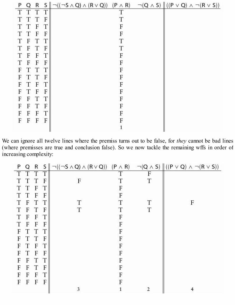
We can ignore all twelve lines where the premiss turns out to be false, for they cannot be bad lines(where premisses are true and conclusion false). So we now tackle the remaining wffs in order ofincreasing complexity:

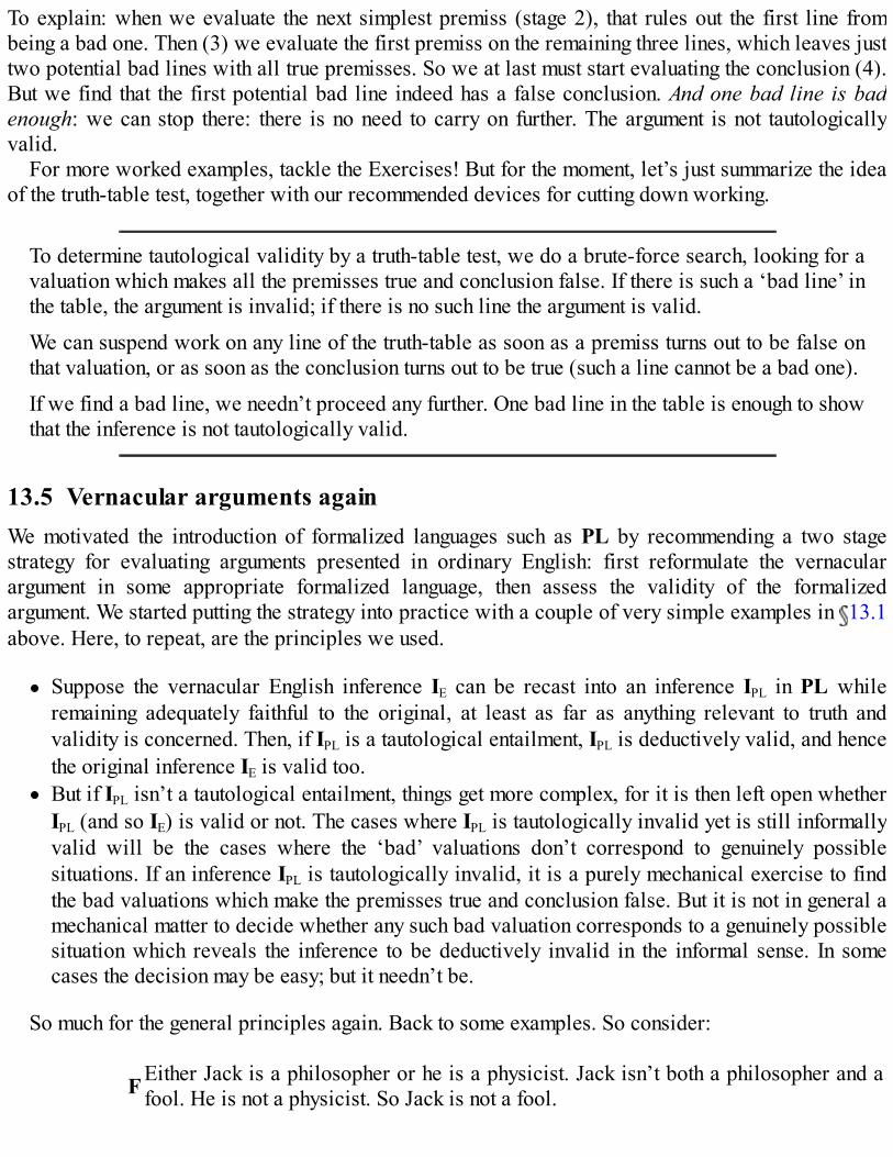
To explain: when we evaluate the next simplest premiss (stage 2), that rules out the first line frombeing a bad one. Then (3) we evaluate the first premiss on the remaining three lines, which leaves justtwo potential bad lines with all true premisses. So we at last must start evaluating the conclusion (4).But we find that the first potential bad line indeed has a false conclusion. And one bad line is badenough: we can stop there: there is no need to carry on further. The argument is not tautologicallyvalid.

For more worked examples, tackle the Exercises! But for the moment, let’s just summarize the ideaof the truth-table test, together with our recommended devices for cutting down working.

To determine tautological validity by a truth-table test, we do a brute-force search, looking for avaluation which makes all the premisses true and conclusion false. If there is such a ‘bad line’ inthe table, the argument is invalid; if there is no such line the argument is valid.

We can suspend work on any line of the truth-table as soon as a premiss turns out to be false onthat valuation, or as soon as the conclusion turns out to be true (such a line cannot be a bad one).

If we find a bad line, we needn’t proceed any further. One bad line in the table is enough to showthat the inference is not tautologically valid.

13.5 Vernacular arguments againWe motivated the introduction of formalized languages such as PL by recommending a two stagestrategy for evaluating arguments presented in ordinary English: first reformulate the vernacularargument in some appropriate formalized language, then assess the validity of the formalizedargument. We started putting the strategy into practice with a couple of very simple examples in 13.1above. Here, to repeat, are the principles we used.

Suppose the vernacular English inference IE can be recast into an inference IPL in PL whileremaining adequately faithful to the original, at least as far as anything relevant to truth andvalidity is concerned. Then, if IPL is a tautological entailment, IPL is deductively valid, and hencethe original inference IE is valid too.But if IPL isn’t a tautological entailment, things get more complex, for it is then left open whetherIPL (and so IE) is valid or not. The cases where IPL is tautologically invalid yet is still informallyvalid will be the cases where the ‘bad’ valuations don’t correspond to genuinely possiblesituations. If an inference IPL is tautologically invalid, it is a purely mechanical exercise to findthe bad valuations which make the premisses true and conclusion false. But it is not in general amechanical matter to decide whether any such bad valuation corresponds to a genuinely possiblesituation which reveals the inference to be deductively invalid in the informal sense. In somecases the decision may be easy; but it needn’t be.

So much for the general principles again. Back to some examples. So consider:

F Either Jack is a philosopher or he is a physicist. Jack isn’t both a philosopher and afool. He is not a physicist. So Jack is not a fool.

Translating this into PL, using ‘P’ for ‘Jack is a philosopher’, ‘Q’ for ‘Jack is a physicist’, ‘R’ for‘Jack is a fool’, we get an argument which can be symbolized

F′ (P ∨ Q), ¬(P ∧ R), ¬Q ∴ ¬R

Is this tautologically valid? If we first evaluate the conclusion (1), and then (2) the simplest premisson the potentially bad lines (i.e. where the conclusion is false) we are left with just two remainingpotential bad lines. Finishing the job (3) gives us

There is no line where the premisses are true and the conclusion false: so the argument istautologically valid. Hence the argument (as encoded in PL) is plain valid. But is the translationaccurate? Perhaps the first premiss is intended as an exclusive disjunction. However, this wouldn’t infact make a difference to the argument’s tautological validity (check that claim). So on either reading,the original argument is valid too.

What about this argument:

GIt is not the case that either Jack or Jill will be at the party. At least one of Jack andJames will be at the party. Hence it isn’t the case that James and not Jill will be at theparty.

Using the obvious translation, and setting out a truth-table (with the same ‘con-clusion-first’ short cut)we get:

In this case, there is a ‘bad line’. So the argument is not tautologically valid. And the bad assignmentwhere P ⇒ F (Jack won’t be at the party) and Q ⇒ F (Jill won’t be there) and R ⇒ T (James is at theparty) is evidently a genuine possibility – so we’ve found a way the premisses could be true and theconclusion false: the PL argument is invalid. Assuming that there are no worries about the translation,the original argument is invalid too.

Consider thirdly this example:

H

Jill’s either in the library or she’s in the coffee bar. And she’s either not in the library,or she’ll be working on her essay. It sure isn’t the case that she’s there in the coffeebar but not talking to her friends. So she’s either working on her essay or talking tofriends.

Is the inference here valid? Read the PL atoms to encode the following messages:

P: Jill is in the library.Q: Jill is in the coffee bar.R: Jill is working on her essay.S: Jill is talking to her friends.

Then a possible translation for the first premiss is simply ‘(P ∨ Q)’ – for after all, the premissesdon’t rule the coffee bar being in the library! If we take the ‘And’ at the beginning of the secondpremiss as just stylistic glue without logical function, then that premiss translates as ‘(¬P ∨ R)’. Thethird premiss translates as ‘¬(Q ∧ ¬S)’, though we lose in translation the rhetorical flourish of ‘Itsure isn’t the case that’ when we replace it by plain negation, and we also lose any fine differences oftone between ‘but’ and plain conjunction. Finally, we could translate the conclusion as ‘(R ∨ S)’. So,one rendition of the original argument into PL is:

H′ (P ∨ Q), (¬P ∨ R), ¬(Q ∧ ¬S) ∴ (R ∨ S)

But compare 13.4 D: the premisses here do tautologically entail the conclusion (for recall, the orderin which premisses are presented can’t make any difference to questions of validity). So the PLinference is a valid one. Hence assuming the adequacy of the translation, the original argument is

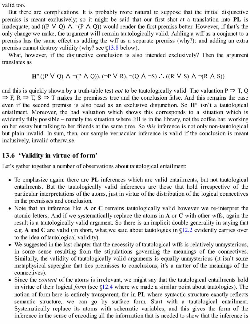
valid too.But there are complications. It is probably more natural to suppose that the initial disjunctive

premiss is meant exclusively; so it might be said that our first shot at a translation into PL isinadequate, and ((P ∨ Q) ∧ ¬(P ∧ Q)) would render the first premiss better. However, if that’s theonly change we make, the argument will remain tautologically valid. Adding a wff as a conjunct to apremiss has the same effect as adding the wff as a separate premiss (why?): and adding an extrapremiss cannot destroy validity (why? see 13.8 below).

What, however, if the disjunctive conclusion is also intended exclusively? Then the argumenttranslates as

H″ ((P ∨ Q) ∧ ¬(P ∧ Q)), (¬P ∨ R), ¬(Q ∧ ¬S) ∴ ((R ∨ S) ∧ ¬(R ∧ S))

and this is quickly shown by a truth-table test not to be tautologically valid. The valuation P ⇒ T, Q⇒ F, R ⇒ T, S ⇒ T makes the premisses true and the conclusion false. And this remains the caseeven if the second premiss is also read as an exclusive disjunction. So H″ isn’t a tautologicalentailment. Moreover, the bad valuation which shows this corresponds to a situation which isevidently fully possible – namely the situation where Jill is in the library, not the coffee bar, workingon her essay but talking to her friends at the same time. So this inference is not only non-tautologicalbut plain invalid. In sum, then, our sample vernacular inference is valid if the conclusion is meantinclusively, invalid otherwise.

13.6 ‘Validity in virtue of form’Let’s gather together a number of observations about tautological entailment:

To emphasize again: there are PL inferences which are valid entailments, but not tautologicalentailments. But the tautologically valid inferences are those that hold irrespective of theparticular interpretations of the atoms, just in virtue of the distribution of the logical connectivesin the premisses and conclusion.Note that an inference like A or C remains tautologically valid however we re-interpret theatomic letters. And if we systematically replace the atoms in A or C with other wffs, again theresult is a tautologically valid argument. So there is an implicit double generality in saying thate.g. A and C are valid (in short, what we said about tautologies in 12.2 evidently carries overto the idea of tautological validity).We suggested in the last chapter that the necessity of tautological wffs is relatively unmysterious,in some sense resulting from the stipulations governing the meanings of the connectives.Similarly, the validity of tautologically valid arguments is equally unmysterious (it isn’t somemetaphysical superglue that ties premisses to conclusions; it’s a matter of the meanings of theconnectives).Since the content of the atoms is irrelevant, we might say that the tautological entailments holdin virtue of their logical form (see 12.4 where we made a similar point about tautologies). Thenotion of form here is entirely transparent; for in PL where syntactic structure exactly reflectssemantic structure, we can go by surface form. Start with a tautological entailment.Systematically replace its atoms with schematic variables, and this gives the form of theinference in the sense of encoding all the information that is needed to show that the inference is

tautologically valid. And instances of this schematic form got by systematically substituting wffsfor the variables will all be tautologically valid.

Note, that last point helps us see exactly how the truth-table test relates to the informal technique forthe evaluation of inferences that we described in Chapter 4. Looking for a ‘bad line’ in a table is astripped-down version of looking for a counterexample. To explain: recall that a counterexample isan inference of the same form as the target inference up for assessment, which has true premisses anda false conclusion. In the case of a PL argument, that would mean abstracting away from theparticular atoms and then finding a substitution instance of the resulting schematic form with truepremisses and a false conclusion. But in PL, all that matters for the truth of premisses and falsity ofconclusion is the values of the atoms. So what ultimately matters about a counterexample is the valuesthe atoms take in it. We can therefore streamline things by skipping the step of actually writing downthe full counterexample and just latch on to the corresponding valuation of the atoms which makes thepremisses true and conclusion false. So in PL terms, looking for a counterexample comes down tolooking for a ‘bad line’ in the truth-table.

Now, as we noted in Chapter 4, failing to find a counterexample doesn’t normally demonstratevalidity. But in the special case of PL arguments, we can do a systematic search through all therelevantly different types of counterexample – i.e. all the different valuations of atoms that theyproduce. So in this special case, failure to find a counterexample, i.e. failure to find a bad valuation,does demonstrate validity.

To return to the point about ‘form’:

We complained before ( 3.6) about over-generalizing the thought that valid arguments are validbecause of their form. But, just as the concept of a tautology gives sharp content to the idea oftruth-in-virtue-of-form ( 12.4), the concept of tautological entailment gives a sharp content tothe idea of validity-in-virtue-of-form for one class of arguments.

As applied to arguments couched in PL, then, the idea of validity-in-virtue of form is clear-cut. Whatof arguments framed in English? Well, in so far as a vernacular argument can be well represented by atautologically valid PL translation, it too might readily be counted as tautologically valid and so, inthe explained sense, valid in virtue of form. (But questions of translation can be rather indeterminate,so the question whether a PL tautological entailment adequately captures the original vernacularargument can in turn be rather indeterminate.)

13.7 and ‘∴’That’s the main business of this chapter done. However, there’s another bit of standard shorthandsymbolism we really should introduce and comment on. Then in the next section we’ll use thesymbolism in stating some general results about tautological validity. (But by all means skip this andthe next section on a first reading).

It is standard to abbreviate the claim that the wffs A1, A2, …, An tautologically entail C by writing

(1) A1, A2, …, An C

(The symbol ‘ ’ here is often called the ‘double turnstile’ – and perhaps a useful mnemonic is to think

of it as made up by superimposing the two ‘t’s from ‘tauto-logical’.)Note, this symbol is being added to English. It is a metalinguistic shorthand for talking about the

relationship of some wffs in PL, and it doesn’t belong to PL itself. This point can get obscuredbecause it is both convenient and absolutely conventional to write, e.g.

(2) (P ∨ Q), ¬P Q

rather than write (as we should do, since we are talking metalinguistically)

(3) ‘(P ∨ Q)’, ‘¬P’ ‘Q’

In other words, it is conventional to take ‘ ’ as – so to speak – generating its own quotation marks.There is a very important contrast, then, between (2) and

(4) (P ∨ Q), ¬P ∴Q

(4) is an argument couched in some dialect of PL. So it makes three assertions, with the inferencemarker ‘∴’ signalling that the third assertion is being inferred from the other two. By contrast, (2) isnot an argument at all, it is a single statement made in shorthand English. It’s short for

(2′) The PLinference whose premisses are ‘(P ∨ Q)’ and ‘¬P’ and whose conclusion is‘Q’ is tautologically valid.

So don’t confuse ‘ ’ with ‘∴’!Finally, note again that (1) says that C is always true, on the condition that the Ai are true: so

(5) C

is naturally read as saying that C is true on no condition at all, i.e. that C is a tautology.

13.8 Some simple metalogical resultsIn 13.1–5, we’ve demonstrated a number of logical results, showing that various arguments areeither tautologically valid or invalid. Finally in this chapter, we go up a level, so to speak, and givesome metalogical results – i.e. results about the idea of tautological validity.

First, some further terminology that will come into its own later:

A set of PL wffs A1, A2, …, An is satisfiable or tautologically consistent if there is at least onepossible valuation of the relevant atoms which makes the wffs all true together. The set isotherwise unsatisfiable or tautologically inconsistent.

To start, note that

(i) A1, A2, …, An C if and only if A1, A2, …, An, ¬C are tautologically inconsistent.

This is immediate. A1, A2, …, An, C if and only if there is no valuation which makes the Ai true and Cfalse, i.e. just when there is no valuation which makes the Ai and ¬C all true, i.e. just when that set ofwffs is unsatisfiable.

Next, note three more results:

(ii) For any B, if A1, A2, …, An C then A1, A2, …, An, B C.(iii) If C is a tautology, then A1, A2, …, An C for any Ai.

(iv) If the wffs A1, A2, …, An are tautologically inconsistent, then A1, A2, …, An C for anyC.

If a valuation of the relevant atoms which makes the Ai all true makes C true as well, then a valuationwhich makes the Ai all true and B as well will still make C true (note, if any of the atoms in B are newones, their values cannot affect the values of the other wffs – see 9.6). In other words, (ii) addingfurther premisses cannot destroy a tautological entailment. Again, if C is true on any valuation of itsatoms, then it is true on any valuation of a wider collection of atoms, and so true on any valuationwhich makes the Ai true. Hence (iii) a tautology is tautologically entailed by any bunch of premisses.Checking (iv) is left as an exercise. (These three results reflect the fact that tautological validity is a‘classical’ notion of validity in the sense we explored in 6.1. Tautologically valid inference doesn’trequire any relation of relevance between the premisses and the conclusion.)

Next, recall the notion of truth-functional equivalence introduced in 11.6. A and B are equivalentsjust if they take the same value on all valuations of their atoms. So whenever A is true, B is, and viceversa. Hence we have

(iv) A and B are equivalents just when A B and B A.

And finally let’s note a result that justifies the use of reductio ad absurdum arguments to establishtautological entailments (for the general idea of such arguments, see again 5.4):

(v) If C is a contradiction, and A1, A2, …, An, B C, then A1, A2, …, An, ¬B

Suppose A1, A2, …, An, B C. Then whenever A1, A2, …, An and B are all true, C is true too. But if C isa contradiction, C is never true on any valuation. So given C is a contradiction, then A1, A2, …, An andB can never all be true together on any valuation. But if A1, A2, …, An and B can never be true together,then whenever A1, A2, …, An are true, B is false. Which shows, as we wanted, that A1, A2, …, An ¬B.

13.9 Summary• Given an argument involving just ‘and’, ‘or’, ‘not’ as its relevant logical materials, we can

evaluate it as follows:

1. Represent the argument in PL using ‘∧’, ‘∨’ and ‘¬’ as the connectives.2. Consider all the possible ways of assigning truth-values to the atoms in the premisses and

conclusion.3. Work out in each case (for each possible assignment) the truth-values of the premisses and

conclusion of the argument.

4. Ask: Is there a bad assignment, i.e. one that makes the premisses all true and yet theconclusion false?

5. If there is no bad assignment, then the argument is tautologically valid. If there is a badassignment, then the argument is tautologically invalid.

• Steps (2) to (5) involve an entirely mechanical procedure; a computer can test whether aninference presented in PL is tautologically valid.

1. As before, we are assuming that we are interpreting atoms of PL to express the sort ofpropositions where are determinately true or false. Tautological validity implies plainvalidity. Tautological invalidity does not always imply plain invalidity, but means that theoriginal argument, if valid at all, must depend for its validity on something other than thedistribution of the propositional connectives in the premisses and conclusion.

2. The test procedure, however, can be speeded up if we note that a line on the truth-table whereany premiss is false or the conclusion is true cannot be a bad line. Such lines can be ignoredin the search for bad assignments.

3. We introduced the symbol ‘ ’ as an augmentation of English, to express the relation oftautological entailment. It is important to distinguish the meta-linguistic ‘ ’ from the object-language inference marker ‘∴’.

Exercises 13A Use the truth-table test to determine which of the following arguments are tautologically valid:

1. ¬(P ∨ Q) ∴ ¬P2. (P ∧ Q) ∴ (P ∨ ¬Q)3. (P ∨ ¬Q), ¬P ∴ ¬¬Q4. (P ∧ S), ¬(S ∧ ¬R) ∴ (R ∨ ¬P)5. P, ¬(P ∧ ¬Q), (¬Q ∨ R) ∴ R6. (P ∨ Q), ¬(P ∧ ¬R), (R ∨ ¬Q) ∴ R7. (¬P ∨ ¬(Q ∨ R)), (Q ∨ (P ∧ R)) ∴ (¬P ∨ Q)8. (P ∨ Q), ¬(Q ∧ ¬¬R) ∴ ¬(R ∨ P)9. (P ∧ (Q ∨ R)) ∴ ((P ∧ Q) ∨ (P ∧ R))

10. (P ∨ Q), (¬P ∨ R), ¬(Q ∧ S) ∴ ¬(¬R ∧ S)

B Evaluate the following arguments:

1. Either Jack went up the hill or Jill did. Either Jack didn’t go up the hill or the water got spilt.Hence, either Jill went up the hill or the water got spilt.

2. It isn’t the case the Jack went up the hill and Jill didn’t. It isn’t the case that Jill went up thehill and the water got spilt. So either Jack didn’t go up the hill or the water got spilt.

3. Either Jack is lazy or stupid. It isn’t true that he is both lazy and a good student. Either Jackisn’t a good student or he isn’t stupid. Hence he isn’t a good student.

4. Either Jill hasn’t trained hard or she will win the race. It isn’t true that she’ll win the race andnot be praised. Either Jill has trained hard or she deserves to lose. Hence either Jill will bepraised or she deserves to lose.

C (Now read 13.7–8 if you took up the invitation to skip them on a first reading.) Which of thefollowing are true; which false; and why?

1. Any two tautologies are truth-functionally equivalent.2. If A tautologically entails C, then A entails any wff truth-functionally equivalent to C.3. If A and B tautologically entail C and B is a tautology, then A by itself tautologically entails

C.4. If A B, then ¬A ¬B.5. If A B, then ¬B ¬A.6. If A is a contradiction, then A B, for any B.7. If the set of wffs A1, A2, …, An is unsatisfiable, the set ¬A1, ¬A2, …, ¬An is satisfiable.8. If the set of wffs A1, A2, …, An is unsatisfiable, then A1, A2, …, An B, for any B.9. If A C, then (¬A ∨ C).

10. If A, B, C are tautologically inconsistent, then A (¬B ∨ ¬C).11. If A, B are tautologically inconsistent, so are ¬A, ¬B.12. If the wffs A, B together make a satisfiable set, and B, C do too, then the wffs A, C together

make a satisfiable set.

Interlude

Propositional logic

Let’s review the state of play again:

We have explained why it can be advantageous to adopt a two-stage strategy in logical theory –first translating inferences into a well-designed artificial language (eliminating obscurity andambiguity), and then evaluating the neatly regimented results.We have seen how to execute the first stage of this strategy in a very plausible and attractive wayfor arguments whose essential logical materials are the propositional connectives ‘and’, ‘or’ and‘not’, by deploying the artificial truth-functional language PL.We then developed a tight definition of ‘tautological validity’ for arguments in PL; this isvalidity in virtue of the distribution of the connectives. And we have seen how we canmechanically test for tautological validity, by the truth-table test.We are assuming we are interpreting atoms of PL to express the sort of propositions where aredeterminately true or false. Then, if an argument is tautologically valid, it is valid in the informalsense – though not always vice versa.

Along the way, we have started the work of tidying some of the loose ends we noted in the lastInterlude.

We acknowledged in the previous Interlude that we hadn’t given a very sharp characterization ofthe general notion of deductive validity. We now, at any rate, have a very clear notion oftautological validity that captures the intuitive notion as applied to one class of arguments.We also acknowledged earlier that we hadn’t given any clear account of the idea of aproposition, nor of what counts as the ‘logical form’ of a proposition or the ‘pattern’ of aninference. But we can at least now talk crisply and accurately about forms of PL wffs orschematic patterns of PL inferences: we can display such patterns by replacing atoms withmetalinguistic variables. The surface forms of PL wffs encode all the semantic facts (about thedistribution of connectives) that matter for the tautological validity of PL inferences,transparently and without any ambiguity. So we don’t need to dig any deeper. We don’t need hereany murkier notion of ‘underlying’ logical form. Nor indeed need we fuss about distinguishing(interpreted) wffs from the propositions they express.

Since PL is expressively adequate – i.e. has the resources to express any possible truth-functionalway of combining atoms – there’s a good sense in which our discussion so far covers the whole of thelogic of truth-functions. Something that we haven’t talked about yet is how we might express proofs(chains of tautological valid inference steps) in PL. But in a way, we don’t need to. The whole pointof using proofs, recall, is to enable us to warrant complex inferences by breaking down the big

inference step from premisses to conclusion into a number of smaller steps, each one of which isindubitably a valid move. However, we’ve just found a nicely mechanical and direct way ofdemonstrating tautological validity. Run a truth-table test and that settles the matter! So why botherwith proofs?

Still, despite the fact that we have – in a sense – already dealt with the whole logic of truth-functions, we are going to proceed over the next few chapters to discuss one more truth-function insome detail. We’ll be examining the so-called ‘material conditional’ which is a truth-functionalconnective that purports to capture (something of) the ordinary language conditional construction ‘ifA, then B’. Conditional propositions of that kind are so important in reasoning that it would be oddindeed to have no way of treating them in our logic. But as we’ll see, they raise a whole raft ofcontentious problems (which is why we’ve kept their treatment sharply separate from the relativelyuncontentious truth-functional logic of ‘and’, ‘or’ and ‘not’).

And despite the fact that it is – in a sense – otiose to lay down formal procedures for chainingtogether PL inferences into proofs, we’ll also spend some time developing what can be regarded asone proof system for propositional logic (though we’ll introduce it as a way of doing truth-tablesfaster). That’s because later, when investigating ‘quantificational logic’ we’ll need to consider proofsystems (there is no equivalent of a mechanical truth-table test for establishing quantificationalvalidity).

Overall, our menu

the basic syntax/semantics of PLtruth-table testingdiscussion of the material conditionala proof system

is, in one form or another, in one ordering or another, pretty much the standard offering in the first partof any elementary text on formal logic. Together, its elements constitute classical propositional logic.

14

PLC and the material conditional

We have seen how to evaluate arguments whose logical materials are the three connectives ‘and’, ‘or’and ‘not’. Can our truth-table techniques be extended to deal with arguments involving the conditionalconstruction ‘if …, then …’? Easily, if the core meaning of the conditional can be captured by a truth-function. The present chapter explores the only candidate truth-function, the so-called materialconditional.

14.1 Why look for a truth-functional conditional?Consider the following simple arguments:

A If Jack bet on Eclipse, then Jack lost his money. Jack did bet on Eclipse. So Jack lost his money.

B If Jack bet on Eclipse, then Jack lost his money. Jack did not lose his money. So Jack did not beton Eclipse.

C If Jack bet on Eclipse, then Jack lost his money. So if Jack didn’t lose his money, he didn’t beton Eclipse.

D If Jack bet on Eclipse, then Jack lost his money. If Jack lost his money, then Jack had to walkhome. So if Jack bet on Eclipse, Jack had to walk home.

E Either Jack bet on Eclipse or on Pegasus. If Jack bet on Eclipse, he lost his money. If Jack bet onPegasus, he lost his money. So, Jack lost his money.

These are all intuitively valid inferences, and are presumably valid in virtue of what ‘if …, then …’means.

Contrast the following arguments:

F If Jack bet on Eclipse, then Jack lost his money. Jack lost his money. So Jack bet on Eclipse.

G If Jack bet on Eclipse, then Jack lost his money. Jack did not bet on Eclipse. So Jack did notlose his money.

These are plainly fallacious arguments. The premisses of F can be true and conclusion false; foolishJack may have lost his money by betting on Pegasus, another hopeless horse. For the same reason, thepremisses of G can be true and conclusion false.

It would be good to have a systematic way of evaluating such arguments involving conditionals.Now, on the face of it, ‘if …, then …’ seems to be a connective like ‘… and …’ and ‘… or …’, atleast in respect of combining two propositions to form a new one. So the obvious question is: can wedirectly extend our techniques for evaluating arguments involving those other two-place connectives

to deal with the conditional as well?Here is a quick reminder how we dealt with arguments involving conjunction and disjunction.

The strategy has two stages: (a) we translate the arguments into PL, and then (b) we evaluate thetranslated arguments, by running the truth-table test.Step (a) presupposes that the ordinary language connectives ‘and’ and ‘or’ are close in their coremeanings to the corresponding connectives of PL. (If the translation were too loose, then averdict on the PL rendition couldn’t be carried back into a verdict on the original argument.)Step (b) depends on the PL connectives being truth-functional. The truth-table test requires that,given any assignment of values to the relevant propositional atoms, we can always work outwhether or not that assignment makes the premisses and conclusion false.

So, if the approach of the previous chapters is to be extended to cover arguments involving theconditional, we need to find some way of rendering conditional statements with tolerable accuracyusing a dyadic truth-function. Can we do the trick?

14.2 Introducing the material conditionalFirst, let’s introduce some entirely standard terminology:

Given a conditional if A then C, we refer to the ‘if’ clause A as the antecedent of theconditional, and to the other clause C as the consequent.An inference step of the form if A then C, A; hence C is standardly referred to by the labelmodus ponens. An inference step of the type if A then C, not-C; hence not-A is called modustollens.

Those two medieval Latin labels for the valid inference-moves in our examples A and B above arestill in such common use that you just need to learn them.

Now, it is quite easy to see that there is only one truth-function which is a serious candidate forcapturing conditionals: this much is agreed on all sides. We’ll first give a longer argument whichidentifies this truth-function by exhaustion of cases, and then a second, shorter, argument for the sameconclusion.

(1) Let’s for the moment informally use the symbol ‘⊃’ to represent a truth-function which is intendedto be conditional-like. The issue is how to fill in the ‘?’s in its truth-table. To repeat, there must be noindeterminate slots left in this table: if there were, we wouldn’t be able to apply the truth-table test tothis conditional connective, and the whole point of the current exercise would be thwarted.

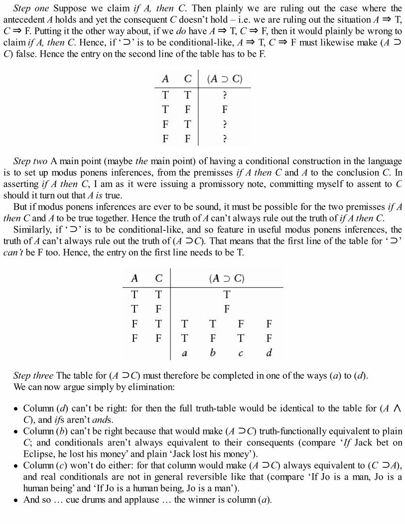
Step one Suppose we claim if A, then C. Then plainly we are ruling out the case where theantecedent A holds and yet the consequent C doesn’t hold – i.e. we are ruling out the situation A ⇒ T,C ⇒ F. Putting it the other way about, if we do have A ⇒ T, C ⇒ F, then it would plainly be wrong toclaim if A, then C. Hence, if ‘⊃’ is to be conditional-like, A ⇒ T, C ⇒ F must likewise make (A ⊃C) false. Hence the entry on the second line of the table has to be F.

Step two A main point (maybe the main point) of having a conditional construction in the languageis to set up modus ponens inferences, from the premisses if A then C and A to the conclusion C. Inasserting if A then C, I am as it were issuing a promissory note, committing myself to assent to Cshould it turn out that A is true.

But if modus ponens inferences are ever to be sound, it must be possible for the two premisses if Athen C and A to be true together. Hence the truth of A can’t always rule out the truth of if A then C.

Similarly, if ‘⊃’ is to be conditional-like, and so feature in useful modus ponens inferences, thetruth of A can’t always rule out the truth of (A ⊃C). That means that the first line of the table for ‘⊃’can’t be F too. Hence, the entry on the first line needs to be T.

Step three The table for (A ⊃C) must therefore be completed in one of the ways (a) to (d).We can now argue simply by elimination:

Column (d) can’t be right: for then the full truth-table would be identical to the table for (A ∧C), and ifs aren’t ands.Column (b) can’t be right because that would make (A ⊃C) truth-functionally equivalent to plainC; and conditionals aren’t always equivalent to their consequents (compare ‘If Jack bet onEclipse, he lost his money’ and plain ‘Jack lost his money’).Column (c) won’t do either: for that column would make (A ⊃C) always equivalent to (C ⊃A),and real conditionals are not in general reversible like that (compare ‘If Jo is a man, Jo is ahuman being’ and ‘If Jo is a human being, Jo is a man’).And so … cue drums and applause … the winner is column (a).

(2) Here’s a shorter argument for the same result. A proposition like If Jo is tall and dark then Jo istall is a necessary truth. Now suppose we translate it PL-style, using ‘⊃’ for a truth-functionalconditional. We get, say, ‘((P ∧ Q) ⊃P)’. This too should be a necessary truth, true in virtue of thetruth-functional meanings of ‘∧’ and ‘⊃’; so it should in fact be a tautology. Consider, therefore, thefollowing truth-table:

In the right-hand column we record the desired result that this conditional is a tautology. The middlecolumns give the values of the antecedent ‘(P ∧ Q)’ and the consequent ‘P’ of that conditional. Andby inspection, to get from the assignments in the middle columns to the values in the final column, atruth-functional conditional (A ⊃ C) must be true when A and C are both true; when A is false, and Ctrue; and when A is false and C false. That fixes three lines of the table. Which leaves the remainingcase when A is true, C is false: in that case (A ⊃ C) must be false (otherwise all conditionals will betautologous). So, again, …

The only candidate that even gets to the starting line as an approximately conditional-like truth-function is the material conditional, defined by:

Why ‘material conditional’? Let’s not worry about that. It’s one of those standard labels that hasstuck around, long after the original connotation has been forgotten. (This truth-function is alsosometimes known as the Philonian conditional, after the ancient Stoic logician Philo, who explicitlydefined it.)

14.3 ‘⊃’ is conditional-likeA bit later ( 14.5 below), we’ll officially add the horseshoe symbol ‘⊃’ to PL, adjusting the syntaxand semantics of that language to get an extended language we’ll call PLC. But for the moment we’llproceed casually, pretend that ‘⊃’ is already part of our language, and quickly check that if wetranslate the examples in 14.1 using ‘⊃’, and run a truth-table test, we get the right verdicts. Thus,

A If Jack bet on Eclipse, then Jack lost his money. Jack did bet on Eclipse. So Jack lost his money.

Translation: (P ⊃ Q), P ∴ Q

Truth-table test:

There are no bad assignments, where all the premisses are true and the conclusion is false: soargument A is tautologically valid as well as being intuitively valid. Skipping the next two simplecases (left as exercises!), we next treat

D If Jack bet on Eclipse, then Jack lost his money. If Jack lost his money, then Jack had to walkhome. So if Jack bet on Eclipse, Jack had to walk home.

Translation: (P ⊃ Q), (Q ⊃ R) ∴ (P ⊃ R)

Truth-table test:

Here we use the now familiar short cut of evaluating the conclusion first, and then only pursuingpotential bad lines, i.e. lines where the conclusion is false. There are no bad lines, so again theargument is tautologically valid.

The next argument exemplifies a common form of inference, often called argument by cases:

E Either Jack bet on Eclipse or on Pegasus. If Jack bet on Eclipse, he lost his money. If Jack bet onPegasus, he lost his money. So, Jack lost his money.

Translation: (P ∨ Q), (P ⊃ R), (Q ⊃ R) ∴ R

Truth-table test:

Again the argument is tautologically valid. So turn next to

F If Jack bet on Eclipse, then Jack lost his money. Jack lost his money. So Jack bet on Eclipse.

We noted before that the inference here is a gross fallacy (traditionally called affirming theconsequent). And the translation of F is tautologically invalid.

Translation: (P ⊃ Q), Q ∴ P

Truth-table test:

The bad line here evidently corresponds to a possible state of affairs – Jack’s not betting on Eclipseyet losing his money all the same – so that confirms that the original argument is plain invalid.

Likewise for

G If Jack bet on Eclipse, then Jack lost his money. Jack did not bet on Eclipse. So Jack did notlose his money.

That’s another horrible fallacy (traditionally called denying the antecedent). Translating and runninga truth-table test confirms this.

In sum, we see from examples A to G that the representation of some ordinary conditionals usingthe truth-functional conditional ‘⊃’ yields the right verdicts about validity and invalidity. So at leastin some respects, ‘⊃’ approximates to the vernacular ‘if …, then …’. In the next chapter, we consider

at length just how close this approximation is.

14.4 ‘If’, ‘only if’, and ‘if and only if’So far, we have only discussed ‘if’ conditionals, i.e. conditionals of the forms

(i) If A then C.

We can also write ‘if’ conditionals in the form

(i′) C, if A.

We take these two versions, without further ado, to be mere stylistic variants. However, there areother kinds of conditional which need to be discussed, in particular ‘only if’ conditionals. Considerthe pair

(ii) A only if C.(ii′) Only if C, then A.

Again, we’ll take this second pair to be trivial variants of each other. The interesting questionconcerns the relation between (i) if A then C and (ii) A only if C.

Consider the following line of thought. Given if A then C, this means that A’s truth implies C, so wewill only have A if C obtains as well – i.e. A only if C holds. Conversely, given A only if C, thatmeans that if A is true, then, willy-nilly, we get C as well. So plausibly, (i) and (ii) imply each other.To take an example, consider

Hi If Einstein’s theory is right, space-time is curved.Hii Einstein’s theory is right only if space-time is curved.

These two do indeed seem equivalent.However, we can’t always equate if A then C with the corresponding A only if C in this simple

way. Compare:

Ii If I drink malt whisky, then I get stupid.Iii I drink malt whisky only if I get stupid.

The latter, but not the former, surely suggests that I have to be stupid first before I make things worseby turning to the whisky. And note another complexity: these conditionals are naturally read to beabout general habits, not about particular situations. But we’ll set aside such quirks of the vernacular.Take the cases where A only if C and if A then C do come to the same; and then both will be renderedinto our extension of PL using the material conditional, by something of the shape (A ⊃ C), with theantecedent and consequent translated appropriately.

Be careful: translating ‘only if’ conditionals does get many beginners into a tangle! The basic ruleis: first put ‘only if’ conditionals into the form A only if C and then replace the ‘only if’ with thehorseshoe ‘⊃’, to get (A ⊃ C). The conditional A if C is of course translated the other way about,

since that is trivially equivalent to if C then A and so is to be rendered by (C ⊃ A).What then about the two-way conditional or biconditional, i.e. A if and only if C (quite often, in

philosophical English, this is written A iff C)? This is equivalent to the conjunction of A only if C andA if C. The first conjunct we’ve just suggested should be translated into our formal language as (A ⊃C); the second conjunct is to be rendered by (C ⊃ A). Hence the whole biconditional can be renderedby ((A ⊃ C) ∧ (C ⊃ A))

However that is a bit cumbersome. And so, although it isn’t necessary, it is common to introduceanother dyadic truth-functional connective, ‘≡’, to replace that construction. This, then, is the so-called material biconditional; and a simple calculation shows that its truth-table will be asdisplayed.

Finally, we should pause to connect the use of conditionals and biconditionals with talk ofnecessary and sufficient conditions. A condition C is necessary for A to hold just when we have Aonly if C. For example, it is a necessary condition of Jo’s being a sister that Jo is female – for Jo is asister only if she is female. But being female isn’t a sufficient condition for being a sister: somefemales are only children. A condition C is sufficient for A to hold just when we have if C then A. Forexample, it is a sufficient condition for Jo’s being a sister that she is a female twin – for if Jo is afemale twin, then she is a sister. But being a female twin isn’t a necessary condition for being a sister:some sisters aren’t twins. Finally, C is a necessary and sufficient condition for A just when A if andonly if C.

14.5 The official syntax and semantics of PLCThe material conditional – like any truth-function – can be expressed using the existing resources ofPL. For example it is easily checked that (¬A ∨ C) has the right truth-table to do the job. Likewise¬(A ∧ ¬C) has the same truth-table.

Similarly the material biconditional can be expressed using ‘∧’, ‘∨’ and ‘¬’. For example, wecould directly conjoin two translations of if A then C and if C then A to get something of the form((¬A ∨ C) ∧(¬C ∨ A)). Or looking at the truth-table for the biconditional, we see that ((A ∧ C)∨(¬A ∧ ¬C)) also has the right table. So we certainly don’t need to add special symbols for theconditional or biconditional.

But there are trade-offs between various kinds of simplicity here. On the one hand, there is thepleasing economy of having just three connectives in our language: the cost is that the translation ofconditionals and biconditionals into standard PL isn’t particularly pretty. On the other hand, if weadd new symbols for the conditionals, we thereby get neater translations: the cost will be that whenwe develop formal proof devices for dealing with arguments things get a bit more complicated (e.g.we need more inference rules). On balance, however, it is worth taking the second trade: so we’llnow officially expand PL by adding two new connectives for the material conditional andbiconditional. We’ll call the new language PLC. Its additional syntactic and semantic rules should beobvious, but here they are, for the record.

Syntax The full alphabet of PLC is the same as that for PL (see 8.1), with the addition of the twosymbols ‘⊃’ and ‘≡’.

The rules for what counts as an atomic wff in PLC stay the same. But we need add two new rulesfor building complex molecular wffs with ‘⊃’ and ‘≡’. Syntactically, however these behave like theother dyadic connectives. So the rules (in short form) are W1 to W4 as before ( 8.1), plus the twonew rules:

(W1) Any atomic wff is a wff.(W2) If A is a wff, so is ¬A.(W3) If A and B are wffs, so is (A ∧ B).(W4) If A and B are wffs, so is (A∨ B).(W5) If A and B are wffs, so is (A ⊃ B).(W6) If A and B are wffs, so is (A≡ B).(W7) Nothing else is a wff.

Semantics We’ll say quite a bit more about the pros and cons of the translation of ‘⊃’ as ‘if’ in thenext chapter. Here we’ll concentrate on valuations (see 9.3). The rules for evaluating wffs with theold three connectives stay the same, of course. So we just need to add:

(P4)For any wffs, A, B: if A ⇒ T and B ⇒ F then (A ⊃ B) ⇒ F; otherwise (A ⊃B) ⇒T.

(P5) For any wffs, A, B: if both A ⇒ T and B ⇒ T, or if both A ⇒ F and B ⇒ F, then (A ≡B) ⇒ T; otherwise (A ≡ B) ⇒ F.

In Chapter 9, we gave rules in this style first and then summed them up in truth-tables. This time,we’ve already given the truth-tables for ‘⊃’ and ‘≡’, and these new semantic rules evidently reflectthose tables.

Finally, just for the record, the notions of a tautology and of tautological entailment are defined forPLC exactly as they were for PL. A PLC wff is a tautology if it is true on all valuations of its atoms;a PLC inference is tautologically valid if there is no valuation of the atoms in the premisses and

conclusion which makes the premisses true and conclusion false.

14.6 , ‘∴’, ‘⊃’, ‘≡’, and ‘→’Recall that in 13.7 we drew a very sharp distinction between the object language inference marker‘∴’ and the metalinguistic sign ‘ ’ for the entailment relation. We now have another sign we must alsodistinguish very clearly from both of these, namely the object language conditional ‘⊃’. Let’s spellthings out carefully.

As we stressed before

(1) (P ∧ Q) ∴Q

is a mini-argument expressed in PL (or in PLC, since this extended language includes the originalone). Someone who asserts (1), assuming that some content has been given to the atoms, is assertingthe premiss, asserting the conclusion, and indicating that the second assertion is based on the first.Compare the English Jack is a physicist and Jill is a logician. Hence Jill is a logician.

By contrast

(2) ((P ∧ Q) ⊃Q)

is a single proposition in PLC; someone who asserts (2) asserts neither ‘(P ∧ Q)’ nor‘Q’. Comparethe English If Jack is a physicist and Jill is a logician, then Jill is a logician.

(3) (P ∧ Q) Q

is another single proposition, but this time in our extended English metalanguage, and the PLC wffsthere are not used but mentioned. For (3) just abbreviates the English

(3′) ‘(P ∧ Q)’ tautologically entails ‘Q’.

Note too the difference between the grammatical category of the PLC connective ‘⊃’ and theEnglish-augmenting sign ‘ ’. The horseshoe sign is a connective, which needs to be combined withtwo sentences (wffs) to make a compound sentence. The double turnstile expresses a relationbetween a premiss (or a set of premisses) and a conclusion, and needs to be combined with twodenoting expressions referring to wffs (or sets of wffs) to make a sentence.

There’s a bad practice of blurring these distinctions by talking, not of the ‘material conditional’,but of ‘material implication’, and then reading (A ⊃ B) as ‘A materially implies B’. If we also read A B as ‘A logically implies B’, this makes it sound as if (A ⊃ B) is just the same sort of claim as A

B, only weaker. But not so. Compare (2) and (3) again: one involves an object-language connective,the other a metalanguage relation.

The following important result, however, does link ‘logical implication’ in the sense of entailmentto ‘material implication’:

E/C A C if and only if (A ⊃ C).

Or in plain words: the one premiss argument A ∴ C is tautologically valid iff (i.e. if and only if) the

corresponding material conditional (A ⊃ C) is a tautology.

Proof: A C, i.e. A ∴ C is tautologically valid,iff there is no assignment of values to the atoms which appear in A and C which makes A true and C

false (by definition),i.e. iff there is no assignment of values to the atoms which appear in A and C which makes (A ⊃ C)

false (by the truth-table for ‘⊃’),i.e. iff every assignment of values to the atoms which appear in A and C makes (A ⊃ C) true,i.e. iff (A ⊃ C) is a tautology (by definition).

By similar reasoning, we can show that the argument A1, A2, …, An ∴ C is valid just when {(A1 ∧ A2

∧ … ∧ An) ⊃ C}, properly bracketed, is a tautology.Here’s a related result, relating equivalence to the biconditional:

E/B A and C are truth-functionally equivalent if and only if (A ≡ C).

Or in plain words: two wffs A and C have the same truth-table if and only the corresponding singlewff (A ≡ C) is a tautology.

Proof: A and C are truth-functionally equivalentiff every assignment of values to the atoms which appear in A and C gives the same values to A and

to C (by definition),i.e. iff every assignment of values to the atoms which appear in A and C makes (A ≡ C) true (by the

truth-table for ‘≡’),i.e. iff (A ≡ C) is a tautology (by definition).

Finally, we should note that ‘→’ is very often used as an alternative symbol for the conditional. ButI recommend the convention of using ‘⊃’ when the truth-functional material conditional is definitelymeant, keeping ‘→’ for more general use.

14.7 SummaryThe only truth-functional connective that is a candidate for translating the conditional of ordinarydiscourse is the so-called material conditional. If we represent this connective by ‘⊃’, then (A⊃ C) is true just when A is false or C is true.A number of ordinary-language arguments using conditionals can be rendered using ‘⊃’ whilepreserving their intuitive validity/invalidity.In many cases, corresponding pairs of the form if A then C and A only if C are equivalent. (Butof course if A then C and only if A then C are not equivalent and their conjunction yields abiconditional.)The only truth-functional connective that is a candidate for translating the biconditional A if andonly if C is the material biconditional. Representing this by ‘≡’, (A ≡ C) is true just when A andC are both true or both false.Since PL is expressively complete, we don’t need to add new symbols to the language toexpress the material conditional and material biconditional. But it is convenient to do so. The

extended language, with the symbols ‘⊃’ and ‘≡’ added in the obvious ways, will be termedPLC.It is important to distinguish the metalinguistic ‘ ’ from the object-language conditional ‘⊃’ andthe object-language inference marker ‘∴’.

Exercises 14A Given

‘P’ expresses Plato is a philosopher‘Q’ expresses Quine is a philosopher‘R’ expresses Russell is a philosopher‘S’ expresses Socrates is a philosopher

translate the following into PLC as best you can:

1. Quine is a philosopher only if Russell is.2. If either Quine or Plato is a philosopher, so is Russell.3. Only if Plato is a philosopher is Russell one too.4. Quine and Russell are both philosophers only if Socrates is.5. Russell’s being a philosopher is a necessary condition for Quine’s being one.6. Plato is a philosopher if and only if Quine isn’t.7. If Plato is a philosopher if and only if Socrates is, then Russell is one too.8. Only if either Plato or Russell is a philosopher are both Quine and Socrates philosophers.9. That Socrates is a philosopher is a sufficient condition for it to be a necessary condition of

Quine’s being a philosopher that Russell is one.10. Quine is a philosopher unless Russell is one.11. Provided that Quine is a philosopher, Russell is one too.

B Use truth-tables to determine which of the following arguments are tautologically valid:

1. P, (P ⊃ Q), (Q ⊃ R) ∴ R2. P, (P ≡ Q), (Q ≡ R) ∴ R3. (P ⊃ R) ∴ ((P ∧ Q) ⊃ R)4. ¬R, (¬P ⊃ R) ∴ P5. (P ≡ R) ∴ (¬R ≡ ¬P)6. (P ⊃ R) ∴ (¬R ⊃ ¬P)7. ¬R, (P ⊃ R), (¬P ⊃ Q) ∴ Q8. (P∨Q), (P ⊃ R), ¬(Q ∧ ¬R) ∴ R9. (R ≡ (¬P∨Q)), ¬(P ∧ ¬R) ∴ ¬(¬R∨Q)

10. (¬P∨Q), ¬(Q ∧ ¬R) ∴ (P ⊃ R)11. (P ∧ ¬R), (Q ⊃ R) ∴ ¬(P ⊃ Q)12. ¬(P ≡ (Q ∧ R)), (S∨¬Q) ∴ ¬(S ⊃ P)

C Which of the arguments that you have just shown to be tautologically valid correspond tointuitively valid arguments when ‘⊃’ is replaced by ‘if …, then …’, and ‘≡’ is replaced by ‘… ifand only if …’?

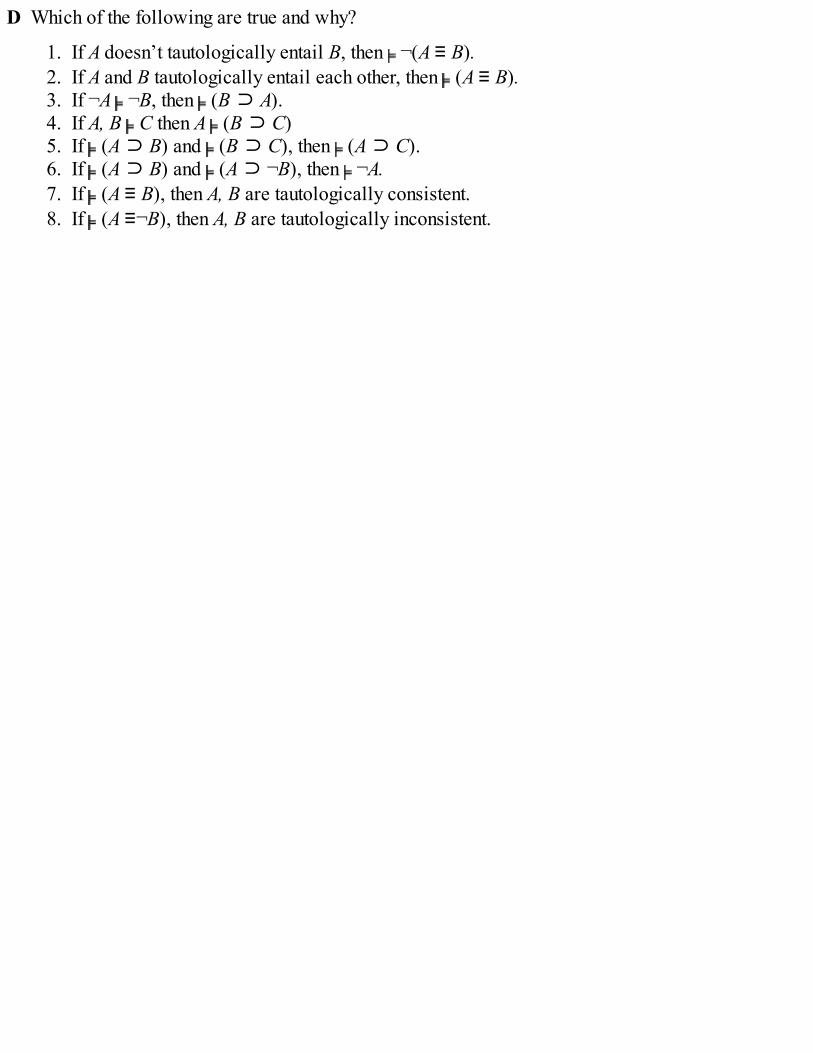
D Which of the following are true and why?

1. If A doesn’t tautologically entail B, then ¬(A ≡ B).2. If A and B tautologically entail each other, then (A ≡ B).3. If ¬A ¬B, then (B ⊃ A).4. If A, B C then A (B ⊃ C)5. If (A ⊃ B) and (B ⊃ C), then (A ⊃ C).6. If (A ⊃ B) and (A ⊃ ¬B), then ¬A.7. If (A ≡ B), then A, B are tautologically consistent.8. If (A ≡¬B), then A, B are tautologically inconsistent.

15

More on the material conditional

The last chapter introduced the material conditional. This chapter discusses more carefully itsrelation with conditionals in ordinary language. We begin by drawing a key distinction between typesof conditional.

15.1 Types of conditionalConsider the following memorable example (due to David Lewis):

(1) If kangaroos had no tails, they would topple over.

How do we decide whether this is true? By imagining a possible world very like our actual world,with the same physical laws, and where kangaroos are built much the same except for the lack oftails. We then work out whether the poor beasts in such a possible world would be unbalanced andfall on their noses. In short, we have to consider not the actual situation (where of course kangaroosdo have tails), but other possible ways things might have been. Let’s call a conditional that invitesthis kind of evaluation (i.e. evaluation by thinking about other ways things might have been) apossible-world conditional.

To introduce another memorable example, compare the following:

(2) If Oswald didn’t shoot Kennedy in Dallas, someone else did.(3) If Oswald hadn’t shot Kennedy in Dallas, someone else would have.

To evaluate (2), note that in the actual world, Kennedy was shot. Someone must have done it. Hence,if not Oswald, someone else. So (2) is true. Now in fact (let’s suppose), Oswald did shoot Kennedy,acting alone. Then, to decide whether (3) is true, we have to consider a non-actual possible world, aworld like this one except that Oswald missed. Keeping things as similar as we can to the actualworld, Oswald would still be acting alone. There would still be no conspiracy, no back-upmarksmen. In such a possible situation, Kennedy would have left Dallas unscathed. Hence (3) isfalse.

Given that they take different truth-values, the possible-world conditional (3) therefore mustdiverge in content from the simple conditional (2).

The logic of possible-world conditionals is beyond the scope of this book, but one thing is clear:possible-world conditionals are not truth-functional. A truth-functional conditional has its actualtruth-value fixed by the actual truth-values of its constituent sentences. By contrast, the truth-value ofa possible-world conditional depends on what happens in other possible scenarios; so its truth-valuecan’t be fixed just by the this-worldly values of the antecedent and consequent.

Hence, quite uncontroversially, the truth-functional rendition can at most be used for conditionalslike (2).

What is very controversial, though, is the range of ‘conditionals like (2)’. Cases like (3) areconventionally called subjunctive conditionals, for supposedly they are couched (according to sometraditional grammars) in the subjunctive mood. (2), and all the conditionals in arguments A to G in 14.1 above, are called indicative conditionals (being framed in the indicative mood). The trouble isthat the intended indicative/subjunctive division seems to carve up conditionals in an unhelpful way.For compare (3) with

(4) If Oswald doesn’t shoot Kennedy in Dallas, someone else will.

Someone who asserts (4) before the event – believing, perhaps, that a well-planned conspiracy isafoot – will after the event assent to (3). Likewise, someone who denies (4) before the event –knowing that Oswald is a loner – will deny (3) after the event. Either way, it seems that exactly thesame type of possible world assessment is relevant for (3) and (4): we need to consider what occursin a world as like this one as possible given that Oswald doesn’t shoot Kennedy there. Plausibly,then, we might well want to treat (3) and (4) as belonging to the same general class of possible-worldconditionals. But, in traditional grammatical terms, (4) is not subjunctive. So the supposed distinctionbetween subjunctive and indicative conditionals divides the past interpretation of (3) from the futureinterpretation of (4) in a pretty unnatural manner.

We can make a related point in passing. Someone who asserts (2) leaves it open whether Oswaldshot Kennedy; but someone who asserts (3) thereby implies that the antecedent is actually false, andthat Oswald didn’t miss. For that reason, conditionals like (3) are often called counterfactualconditionals. But (4) is not a counterfactual in this sense: someone who asserts (4) again leaves itopen whether Oswald will miss. So the counterfactual/non-counterfactual distinction againunnaturally divides (3) from (4).

We can’t pursue these matters further here. The point, to repeat, is that it isn’t obvious exactlywhere and how to draw the line between those possible-world conditionals like (3) which have to beset aside as definitely not apt for a truth-functional treatment, and those ‘indicative’ conditionals like(2) which are still in the running.

15.2 In support of the material conditionalWe noted that the material conditional (like any truth-function) can be expressed with the unaugmentedresources of PL; the two simplest ways of capturing the truth function using the original connectivesare ¬(A ∧ ¬C) and (¬A ∨ C). Do these equivalent ways of expressing the truth-function make it lookmore or less like a conditional? Well, consider the following two lines of thought:

If A then C rules out having A true while C is false; hence, borrowing the PL symbols forbrevity, if A then C implies the corresponding ¬(A ∧ ¬C). Suppose conversely that we believethat ¬(A ∧ ¬C), i.e. that we think that we don’t have A true while C is false. That seems to implythat if A is true, then C won’t be false, or in other words, if A then C. So, apparently, if A then Cimplies and is implied by ¬(A ∧ ¬C). Which is to say that the ordinary language conditional isequivalent to the material conditional.Suppose we hold that if A then C, and put that together with the law of excluded middle (¬A ∨

A). Then we either have ¬A, or we have A and so C. In other words, if A then C implies (¬A ∨C). Conversely, suppose we hold (¬A ∨ C); if A is in fact true, then – since that rules out thefirst disjunct – we can conclude C must be true as well. So, apparently, if A then C implies andis implied by (¬A ∨ C). Which is again to say that the ordinary language conditional isequivalent to the material conditional.

These arguments are enough to lead many logicians to hold that at least some ordinary ‘if …, then …’propositions are fundamentally truth-functional.

15.3 Against identifying vernacular and material conditionalsDo the arguments of the previous section really establish that the core meaning of indicativeconditionals is truth-functional (i.e. that these ordinary language conditionals are materialconditionals)?

Note that a material conditional, a proposition with the same truth-table as (¬A ∨ C), can be trueirrespective of any connection between the matters mentioned by A and C. All that’s required is A isfalse and/or C is true. You might hold that this simple observation is already enough to sabotage theclaim that ordinary ‘if’s can be treated as equivalent to material conditionals. For don’t ‘if’s signalsome kind of real connectedness between the topics of the antecedent and consequent?

No, not always. Suppose I remember that one of Jack and Jill has a birthday in April (I know thatthey threw a party last Easter, but I just can’t recall whose birthday it was celebrating). You say, a bithesitantly, that you think that Jack has an October birthday. So I respond

(1) If Jack was born in October, then Jill was born in April.

Surely in the context that’s a perfectly acceptable conditional, though I don’t for a moment think thatthere is any causal or other connection between the facts about their birth months. All I’m saying isthat either you are wrong about Jack, or else Jill was born in April: i.e., borrowing the PL symbolsagain, I’m just committing myself to

(2) (¬Jack was born in October ∨Jill was born in April).

So it seems that perfectly acceptable conditionals may be no-more-than-material.Of course, when we assert conditionals, we often do think that there is (for example) a causal

connection between the matters mentioned in the antecedent and the consequent (‘If you press thatbutton, it will turn on the computer’). But equally, when we assert disjunctions, it is often because wethink there is some mechanism ensuring that one disjunct or the other is true (‘Either the e-mail willbe sent straight away or you’ll get a warning message that the e-mail is queued’). However, even ifour ground for asserting that disjunction is our belief in an appropriate mechanism relating thedisjuncts, what we actually say is true so long as one or other disjunct holds (exclusively, in ourexample). Likewise, our reason for asserting a conditional may be a belief in some mechanism thatensures that if the antecedent holds the consequent does too. It could still be the case that what we sayis true just so long as the material conditional holds.

So far, the material conditional theory survives. But now compare the following (we’ll borrow‘⊃’ to signal the material conditional in English):

(3) Wordsworth didn’t write Pride and Prejudice. So, (Wordsworth wrote Pride andPrejudice ⊃Wordsworth wasn’t a novelist).

(4) Wordsworth didn’t write Pride and Prejudice. So, if Wordsworth wrote Pride andPrejudice then he wasn’t a novelist.

Grant (3)’s premiss that Wordsworth didn’t write Pride and Prejudice. The conclusion is of the form(A ⊃ C) with a false antecedent, so the conclusion must be true too. Hence the inference in (3) isvalid. That is no more puzzling than the validity of the inference from ¬A to (¬A ∨ C); indeed, (3) ineffect just is that trivial inference. By contrast, the inference in (4)looks decidedly unhappy. Manywill say: its conclusion looks unacceptable (being the author of Pride and Prejudice would surely beenough to make you a novelist!): so how can it validly follow from the true premiss that Wordsworthdidn’t write Pride and Prejudice?

Generalizing, the inference pattern

(M) not-A; so (A ⊃ C)

is unproblematically and trivially reliable. On the other hand, inferences of the type

(V) not-A; so if A then C

strike us as very often unacceptable (for indicative conditionals as well as subjunctive ones).Equating the vernacular conditional in (V) with the material conditional in (M) has the highlyimplausible upshot that the two inference patterns should after all be exactly on a par.

Now we seem to be in a mess. On the one hand, we presented in the last section what seemed agood argument for saying that if A then C implies and is implied by ¬(A ∧ ¬C), and then anothergood argument for saying that if A then C implies and is implied by (¬A ∨ C), where ¬(A ∧ ¬C) and(¬A ∨ C) are just two ways of expressing the material conditional. Yet here, on the other hand,we’ve emphasized what looks to be a very unwelcome upshot of treating ordinary ‘if’s as equivalentto material ‘⊃’s. What to do?

15.4 RobustnessGo back to a remark made in passing in 14.2. I said: when we claim if A then C, we are normallyissuing a promissory note, committing ourselves to assent to C should it turn out that A true.

Now imagine that I currently hold not-A, and on that ground alone hold (¬A ∨ C). Would I in thiscase be prepared to go on to issue a promissory note committing myself to assent to C should it turnout that in fact A after all? No! If it turns out that A, I’d retract my current endorsement of not-A, andso retract the disjunction (¬A ∨ C). Hence, if I accept (¬A ∨ C) – or equivalently (A ⊃ C) – on thegrounds that not-A, then I won’t be prepared to endorse the promissory conditional if A then C.

Let’s say, following Frank Jackson, that my assent to (¬A ∨ C), or equivalently (A ⊃ C), is robustwith respect to A if the discovery that A is true won’t lead me to withdraw my assent. Then the pointwe’ve just made comes to this: if my assent to (¬A ∨ C), or equivalently (A ⊃ C), isn’t robust withrespect to A, I won’t accept the force of the 15.2 argument from (¬A ∨ C) to if A then C.

Exactly similarly, suppose I endorse something of the form ¬(A ∧ ¬C) because I believe ¬A.Again, I’ll take it back if I discover than in fact A holds. So again I won’t accept the force of the 15.2

argument from ¬(A ∧ ¬C) to if A then C.This observation suggests a new account of ordinary, indicative conditionals, an account which

both recognizes the appeal of the arguments in 15.2 yet also recognizes the intuitive distinctionbetween the inferences (M) and (V) that we stressed in 15.3. The suggestion is that ordinaryconditionals are not just material conditionals, rather they are material conditionals presented asbeing robust (i.e. robust with respect to their antecedents).

Let’s explain that more carefully. Compare:

(1) Jack came to the party.(2) Even Jack came to the party.

These plainly differ in overall meaning. And yet it seems that the worldly state of affairs they reportis one and the same, namely Jack’s presence at the party. The difference between (1) and (2) doesn’tseem to reside in what they tell us about the world. Rather, the word ‘even’ functions rather like averbal highlighter – or a verbalized exclamation mark – typically used to signal the speaker’s feelingthat Jack’s presence was surprising or out of the ordinary.

Similarly, compare the following:

(3) Jack came to the party and had a dreadful time.(4) Jack came to the party but had a dreadful time.

Again, the worldly state of affairs these two report seems to be the same. The difference betweenthem is that the use of (4) signals, very roughly, that Jack’s going to the party without enjoying it wasagainst expectation.

Likewise, it is now being suggested that the difference between these –

(5) (Jack came to the party ⊃ Jack had a good time)(6) If Jack came to the party, then he had a good time.

– is again not a difference in what they say about the world. Each is strictly speaking true so long asits antecedent is false and/or consequent true. Rather the difference arises because someone who uses‘if’ signals that their claim is robust with respect to the antecedent. In other words, the speaker whouses (6) rather than (5) undertakes not to withdraw the conditional should it turn out that theantecedent is true and Jack did come to the party.

Go back to that example where I recall the Easter birthday party which shows that one of Jack andJill has an April birthday. We argued that it could be natural to endorse

(7) If Jack was born in October, then Jill was born in April.

That’s nicely in keeping with the current theory, since (in the circumstances) although (7) may be no-more-than-material in propositional content, it is robust.

Now since, on this theory, the core content of if A then C is exactly (A ⊃ C), it is no surprise that –quietly assuming robustness – we can construct plausible arguments as in 15.2, from (A ⊃ C) to if Athen C, as well as vice versa. But note too that, while we can accept the unproblematic inference

(M) not-A; so (A ⊃ C)

we won’t robustly endorse (A ⊃ C) if our ground for believing the material conditional is simply thefalsity of the antecedent. Hence, we won’t want to signal that the conclusion of argument (M) is beingheld robustly. In other words – according to our theory which equates ordinary-language conditionalswith material conditionals signalled as being robust – we won’t want to say something of the form

(V) not-A; so if A then C

Which accords exactly with the point of 15.3.In summary, the ‘robust material conditional’ theory is one theory about ordinary ‘if … then …’

which neatly accommodates both the attractions of the 15.2 arguments for thinking that indicativeconditionals are material conditionals, and also the 15.3 considerations that press against a pureequivalence.

15.5 ‘Dutchman’ conditionalsThe previous section’s theory about indicative conditionals is neat: but is it right? Is asserting aconditional always tantamount to giving a promissory note to accept the consequent should theantecedent turn out to be true? What about the following conditionals? –

(1) If George W. Bush is a great philosopher, then pigs can fly.(2) If George W. Bush is a great philosopher, then I’ll eat my hat.

Or, to take a paradigm example, consider

(3) If George W. Bush is a great philosopher, then I’m a Dutchman.

Here I assert the conditional inviting you to apply modus tollens, i.e. to infer from my assertion if Athen C, together with the obvious truth of not-C, that not-A. And my grounds for asserting theconditional are none other than my belief in not-A. I commit myself to no more than the corresponding(¬A ∨ C). Were I to discover that the antecedent A is in fact true – discover that Bush has a secretother life as the pseudonymous author of some much admired philosophical works – then I’d have totake back my scornful conditionals.

In short, these ‘Dutchman’ conditionals are mere material conditionals which are not robustlyasserted. What does that show?

You could take it as counting against the ‘robust material conditionals’ theory. But equally, youcould take the opposing line. After all, ‘Dutchman’ conditionals do strike us pre-theoretically asexceptional cases, as being a jokey idiom. And our theory explains why: they are conspicuously non-robust, and so offend against one aspect of the usual rules governing the assertion of conditionals,which is why they seem non-standard. So, you might hold that far from being refuted by the behaviourof ‘Dutchman’ conditionals, our theory explains it.

But we can’t pursue this tangled issue any further here. We’ve already followed the twists and turnsof arguments about the nature and variety of conditionals far enough. Two points, however, haveclearly emerged.

First, it should now be clear why, when introducing truth-functional logic, we didn’t attempt to dealwith conditionals right from the start. Rendering ‘if …, then …’ by a truth-function raises complexproblems of a quite different order to the issues raised by treating ‘and’, ‘or and ‘not’ as truth-functions. To clutter the initial discussion of PL inferences with these problems would have beenvery distracting; while to have introduced the material conditional straight off without much commentwould have seemed at best mystifying, at worst a cheat.

Secondly, on the ‘robust material conditional’ theory, the rendition of indicative conditionals by‘⊃’ captures that aspect of the content of ordinary indicative conditionals which has to do withmatters of truth and falsehood, and hence the aspect which logic (the study of truth-preservinginferences) needs to focus on. And we can now see that, on any theory, there is some considerableplausibility in at least treating indicative conditionals as having a truth-functional core, even if thereare other aspects of the use of vernacular conditionals that are missed if we try to insist on a baldequation between ‘if’ and ‘⊃’.

The moral, then, is this:

If you want to be able to regiment arguments involving the vernacular indicative conditional intoa form that you can test using the truth-table test, then there is nothing for it but to use thematerial conditional ‘⊃’. If you want to be able to apply the truth-table test, then the price is thatyou have to re-express the premisses and conclusion using ‘⊃’. The rendition preserves thevalidity/invalidity of arguments in at least some central cases. But arguably the translation is notalways an accurate one (even once we’ve set aside the possible world conditionals foralternative treat-ment). Something – in some cases, you may think, too much – may be lost intranslation.

Whatever you think about all the considerations in this chapter, the material conditional has to comewith the warning use with care.

15.6 SummarySubjunctive’ or ‘counterfactual’ conditionals are possible-world conditionals, and are not truth-functional.Even restricting ourselves to indicative conditionals, there are various valid inferencesinvolving the truth-functional conditional whose ordinary-language counterparts look dubious orpositively invalid.The ‘robust material conditional’ theory gives one possible explanation of some of thesedivergences. (Note, however, the theory is a contentious one!)The material conditional must come with a Logical Health Warning.

Exercises 15

A (a)

The pattern of inference C; so (A ⊃ C) is trivially valid. What about the inference C; so ifA then C? (Consider: given C is true, then it is true whether A is or not, so in particular it istrue if A is. But also compare the inference Bush will win the election; so if there is a hugefinancial scandal involving the Bush family then Bush will win the election.)

(b) The pattern of inference (B ⊃ C); so ((A ∧ B) ⊃ C) is trivially valid. What about theinference if B then C; so if A and B then C? (Con-sider, ‘If you strike this match, it willlight; so if you wet this match and strike it, it will light.’)

B

Consider the variant language PLF whose only one- or two-place connective is ‘⊃’, but whichhas – as well as the usual atoms, ‘P’, ‘Q’, etc. – the additional atomic wff ‘⊥’ which is governedby the semantic rule that it always takes the value F (so there is no option about how to evaluatethis atom).

(a) Show that negation, disjunction, and conjunction can be expressed in PLF. (Hint: start byconsidering material conditionals relating two propositions, one of which is ‘⊥’.)

(b) What does it mean to say that PLF is expressively adequate? Is it true?

(c)

You are familiar with the idea of a one-place truth-functional connective (like negation) and atwo-place connective (like conjunction): so what does it mean to talk of an n-place truth-functional connective? What, then, would be a 0-place truth-functional connective? Can wethink of ‘⊥’ as a 0-place connective?

(The symbol ‘⊥’ is often called the falsum; hence the label ‘PLF’.)

16

Introducing PL trees

In previous chapters we defined what it is for PL (and PLC) inferences to be tautologically valid. Wethen introduced one way of testing for tautological validity, namely the brute force truth-table test,where we search through every assignment of values to the relevant atoms to see if there is one whichmakes the premisses true and the conclusion false. In this chapter, we introduce another way of testingfor tautological validity, using ‘truth trees’. We begin with an informal exploration via examples: andfor the moment we will concentrate on PL inferences (we’ll extend the story to cover conditionals inChapter 18).

16.1 ‘Working backwards’Consider the following argument (here and henceforth you can give the atoms whatever content youlike to make things meaningful):

A (P ∧ ¬Q), (P′ ∧ Q′), (¬P″ ∧ ¬Q″) ∴ R

This is plainly not tautologically valid. But suppose we want to confirm this using a truth-table. Thereare seven different atoms involved in the argument, so using the direct truth-table test would meanwriting down a 128-line table, and checking each valuation until we find a line where we have truepremisses and a false conclusion. Fortunately, slogging through like this is utterly unnecessary. Forconsider the following chain of reasoning.

The inference in A is tautologically invalid if and only if there is a valuation which makes thepremisses true and conclusion false, i.e. a valuation where

(1) (P ∧ ¬Q) ⇒ T(2) (P′ ∧ Q′) ⇒ T(3) (¬P″ ∧ ¬Q″) ⇒ T(4) R ⇒ F

(for the convention of dropping quotes round the wff preceding ‘⇒’, see 10.2: but do remember that(1) etc. are still metalinguistic). (1) will hold just so long as we have both

(5) P ⇒ T(6) ¬Q ⇒ T

since a conjunction is only true if its conjuncts are true. Similarly, to guarantee (2) and (3) we need

(7) P′ ⇒ T(8) Q′ ⇒ T(9) ¬P″ ⇒ T

(10) ¬Q″ ⇒ T

To get these assignments (4) to (10), we just need the following valuation of the seven atoms:

P ⇒ T, P′ ⇒ T, P″ ⇒ F, Q ⇒ F, Q′ ⇒ T, Q″ ⇒ F, R ⇒ F

So we have very speedily located a valuation of the atoms in A, custom designed to make thepremisses true and conclusion false. Hence the inference is indeed tautologically invalid.

What we’ve done here is to ‘work backwards’. Instead of starting with the whole set of possiblevaluations for the atoms, and then working forward through each possibility, calculating the truth-values of the premisses and conclusion as we go, looking for a ‘bad’ valuation all the while, we trystarting from the other end. We suppose for the sake of argument that there is a ‘bad’ valuation wherethe premisses are true and the conclusion false. Then we try to work backwards towards a valuationof the atoms that has that unfortunate consequence. If we can do the trick, then obviously the inferenceis not valid.

A few more simple examples should help make the general strategy clear. So consider thefollowing inference:

B (P ∧ Q), ¬(¬R ∨S) ∴ ¬(R ∧ Q)

This will be invalid if and only if there is a valuation where

(1) (P ∧ Q) ⇒ T(2) ¬(¬R ∨S) ⇒ T(3) ¬(R ∧ Q) ⇒ F

To ensure that (1) holds, we evidently need

(4) P ⇒ T(5) Q ⇒ T

To get (2), we need

(6) (¬R ∨S) ⇒ F

and since a disjunction is false only when both disjuncts are false, that means

(7) ¬R ⇒ F(8) S ⇒ F

And, from (7), that means we need

(9) R ⇒ T

Finally, from (3) we have

(10) (R ∧ Q) ⇒ T

which requires, consistently with what we had before, that

(11) R ⇒ T(12) Q ⇒ T

In sum, then, we have backtracked to the valuation

P ⇒ T, Q ⇒ T, R ⇒ T, S ⇒ F

which is expressly constructed to yield the truth-value assignments (1), (2) and (3), and thus make thepremisses of B true and the conclusion false. Hence this second sample argument is again invalid.

Now consider this even simpler inference:

C (P ∧ ¬Q) ∴ ¬(Q ∧ R)

As before, this is invalid if and only if there is a valuation which makes the premiss true and theconclusion false, i.e. a valuation where

(1) (P ∧ ¬Q) ⇒ T(2) ¬(Q ∧ R) ⇒ F

From the specification (1) we can infer

(3) P ⇒ T(4) ¬Q ⇒ T

Next, (2) implies

(5) (Q ∧ R) ⇒ T

which in turn implies

(6) Q ⇒ T(7) R ⇒ T

But plainly, we can’t make ‘¬Q’ true (as (4) requires), and simultaneously make ‘Q’ true (as (6)requires). Hence the supposition that C is invalid puts contradictory demands on the valuation of therelevant atoms. And if that supposition leads to contradiction, C must be valid after all (that’s a

reductio argument: see 5.4).Even in this last mini-example, the ‘working backwards’ technique saves time as against writing

out an eight-line truth-table. Here’s another example where the saving is even greater:

D ¬(¬P ∨ Q), ¬(¬R ∨ S) ∴ (R ∨ ¬P)

A brute force truth-table evaluation would require examination of the sixteen possible valuations ofthe relevant atoms, and barring short cuts, forty-eight evaluations of wffs. Compare, however, thefollowing simple chain of reasoning. Suppose there is a valuation such that

(1) ¬(¬P ∨ Q) ⇒ T(2) ¬(¬R ∨ S) ⇒ T(3) (R ∨ ¬P) ⇒ F

Now, to get (1) and (2), we need

(4) (¬P ∨ Q) ⇒ F(5) (¬R ∨ S) ⇒ F

Again, for a disjunction to be false, both its disjuncts must be false. So it follows that for (3) to holdwe’d need

(6) R ⇒ F

while for (5) to hold we’d need

(7) ¬R ⇒ F

Contradiction! In sum, a valuation will only make the original premisses of D all true if it makes ‘R’true (as (7) requires), and it will only make the conclusion false if it makes ‘R’ false (as (6) says).That’s impossible. So D must be tautologically valid.

16.2 Branching casesTo summarize so far. Testing an argument for tautological validity is a matter of deciding whetherthere are any ‘bad’ valuations of the relevant atoms, i.e. valuations which make all the premisses trueand yet the conclusion false. One approach (embodied in the truth-table test) is to plod through everypossible valuation, to see if a ‘bad’ one turns up. It is usually quicker, however, to approach the samedecision task from the other end. We assume there is a bad valuation that makes the premisses and theconclusion false, and then work out what this ‘bad’ valuation must look like. If we can do the trick,that shows the entailment doesn’t hold. On the other hand, if working backwards from the assumptionof invalidity leads to contradictory results, then (by a reductio ad absurdum argument) that shows thatthere is no bad valuation after all and the argument is valid.

Unfortunately, however, when following through this new strategy in practice, things are typicallyrather more complicated than our examples so far reveal. Consider next this plainly bogus mini-

argument:

E (P ∨ Q) ∴ P

Working backwards by assuming that the premiss is true and the conclusion is false, we have

(1) (P ∨ Q) ⇒ T(2) P ⇒ F

This time we cannot deduce from (1) the values of ‘P’ and ‘Q’. All that (1) tells us is that (at least)one of these is true, but not which. So here we must consider the possible alternatives in turn. We canperspicuously represent the two cases we need to examine by drawing a forking pathway for ourinferences, thus:

(1) (P ∨ Q) ⇒ T(2) P ⇒ F

(3)

We know that, given (1), at least one of the forking alternatives at line (3) must hold; so we nowexamine the options in turn. The assignment P ⇒ T on the left-hand fork gives one way ofguaranteeing (1). But this alternative has in fact already been ruled out, since we earlier have P ⇒ Fat step (2). Taking the left-hand fork leads to contradiction. Let’s ‘close off’ a path like this where awff is assigned inconsistent values by writing a marker like ‘ ’ at its foot, to signal that we’ve hit anabsurdity. So we get

(1) (P ∨ Q) ⇒ T(2) P ⇒ F

(3)

However, while taking the left-hand fork leads straight to absurdity, there is no contradiction on theright-hand fork. Taking that fork gives us the valuation P ⇒ F, Q ⇒ T which makes the premiss of theargument true and conclusion false. Hence argument E is shown to be invalid.

We will work through some more examples to show how we typically need to trace down forkingalternatives when searching backwards for a ‘bad’ valuation. So consider next the valid ‘disjunctivesyllogism’ inference

F (P ∨ Q), ¬P ∴ Q

Starting by assigning truth to the premisses and falsehood to the conclusion, we have:

(1) (P ∨ Q) ⇒ T

(2) ¬P ⇒ F(3) Q ⇒ F

(4)

At (4) we have begun considering the alternative ways of verifying (1). We don’t know what values‘P’ and ‘Q’ have. But we know that one of them is true. This time we see that the left-hand option isinconsistent with (2), which of course implies that ‘P’ is false; and the right-hand option isinconsistent with (3). So both branches lead to absurdity:

(1) (P ∨ Q) ⇒ T(2) ¬P ⇒ F(3) Q ⇒ F

(4)

Hence there is no consistent way of making the premisses and negation of the conclusion all true; sothe argument is indeed valid.

For another example, consider

G ¬(P ∧ Q), (P ∧ R) ∴ ¬(R ∨ Q)

We start the same way, supposing that the premisses true and conclusion false:

(1) ¬(P ∧ Q) ⇒ T(2) (P ∧ R) ⇒ T(3) ¬(R ∨ Q) ⇒ F

To make these true, we definitely need

But now we can make no more firm deductions. (4) tells us that the conjunction of ‘P’ and ‘Q’ is false,so one of the conjuncts must be false. But we aren’t told which, so we need to consider the alternativepossibilities, thus

Here the left hand fork leads immediately to contradiction, as we already have P ⇒ T at (4). So wemust close off that path with the absurdity marker to indicate that no coherent valuation will emergeon this route, and turn our attention to the right-hand path. On this path, there is no explicitcontradiction yet; however, we still have to deal with the implications of (7). This says that at leastone, though we don’t yet know which, of ‘R’ and ‘Q’ must be true. We again need to consider forkingalternatives, so we’ll get the tree:

The new right-hand fork leads immediately to contradiction, since taking that route would require ‘Q’to be both false and true; hence that branch too can be closed off with an absurdity marker. But theremaining path down, where

P ⇒ T, Q ⇒ F, R ⇒ T

leaves us with a consistent valuation custom designed to make (1), (2) and (3) all hold (check that itdoes!), thus showing G to be invalid.

16.3 Signed and unsigned treesLet’s summarize again. We can test an argument for tautological validity by assuming that theinference is invalid and then ‘working backwards’, trying to find a consistent valuation whichwarrants that assumption. At various points, we may have to consider alternative valuations. Forexample, if we have arrived at (A ∨ B) ⇒ T, then we have to consider the alternatives A ⇒ T and B⇒ T. If, twist and turn as we might, all such alternatives lead in the end to contradictory assignmentsof values to atoms, then we know that the original assumption that the inference is invalid is incorrect.In other words, if all branches of the ‘tree’ on which we set out the working can be closed off withabsurdity markers, then the argument is valid. Conversely, if at least one alternative route through thetree involves no contradiction (even when all the complex wffs are fully unpacked), then theassumption that the argument is invalid is vindicated.

Now, so far, our ‘working backwards’ arguments we’ve been illustrating have been set out in theform of signed trees (we’ll speak of ‘trees’ here even if there is – as in 1 – only a trunk without anybranching). The trees are ‘signed’ in the sense that the wffs that appear on them are all explicitly

assigned a truth-value, either T or F. In the interests of neatness and economy, we are now going tomove to using unsigned trees.

As a major step towards doing this, note that by a couple of simple tricks, we can easily ensure thatevery wff which appears on a ‘working backwards’ tree in fact gets the uniform value T. Here’s how:

Trick one Instead of starting a tree by assuming that the premisses of the argument to be testedare true and the conclusion false, assume that the premisses and the negation of the conclusionare all true.Trick two Thereafter, avoid ever writing something of the form ‘C ⇒ F’ by always jumpinginstead to something of the form ‘¬C ⇒ T’.

So, for example, when we meet on a tree a claim of the kind

(a) ¬(A ∨ B) ⇒ T

don’t proceed via the obvious consequence

(b) (A ∨ B) ⇒ F

to

(c) A ⇒ F(d) B ⇒ F

but instead (trick two) jump straight from (a) to

(c*) ¬A ⇒ T(d*) ¬B ⇒ T

And so on. The resulting ‘T’-only trees are only very slightly less natural than the ‘T-and-F’ treeswe’ve been constructing so far.

Let’s quickly illustrate by re-doing a couple of examples in this style, with ‘T’-only trees: thechanges required are marginal. So return first to

D ¬(¬P ∨ Q), ¬(¬R ∨ S) ∴ (R ∨ ¬P)

Starting this time by assigning truth to the premisses and the negation of the conclusion, and we have:

(1) ¬(¬P ∨ Q) ⇒ T(2) ¬(¬R ∨ S) ⇒ T(3) ¬(R ∨ ¬P) ⇒ T

Now, let’s twice apply the rule just given for negated disjunctions (‘jump from ¬(A ∨ B) ⇒ T to addboth ¬A ⇒ T and ¬B ⇒ T’), and we immediately get

We can close off the tree with an absurdity marker because of (6) and (4): no wff and its negation canbe true together on a valuation. Since the tree starting from the supposition that the premisses andnegation of the conclusion are true leads to contradiction, the argument must be valid. (And why arethere two negation signs at line (4)? Because our rule said that if a negated disjunction is true, theneach negated disjunct is true; and if a disjunct already starts with a negation sign, as in ‘¬R’ in (2),then it acquires another when negated.)

For a second ‘T’-only tree, return to

G ¬(P ∧ Q), (P ∧ R) ∴ ¬(R ∨ Q)

Starting with the assumption that the premisses and negated conclusion are true we get:

The rule applied at (7) relies on the fact that, if a negated conjunction is true, then one or other of theconjuncts must be false (so we have the rule ‘given ¬(A ∧ B) ⇒ T, consider alternatives ¬A ⇒ T and¬B ⇒ T’). Not all branches of this resulting tree lead to absurdity. So there is a coherent way ofmaking the premisses and negated conclusion all true together, and so argument G must betautologically invalid.

It is worth quickly checking that our other sample trees can be rewritten with minimal changes as‘T’-only trees. But why care that we can do this?

Because if we make assignments of truth standard on trees, and avoid ever assigning falsehood,then it isn’t really necessary to keep on writing down ‘⇒ T’ against each and every wff in our back-tracking reasoning. We might as well just let it be understood as ever-present. So from now on, let’ssave time and ink by using ‘T’-only trees and then keep the uniform assignments of truth tacit.Suppressing the explicit assignments leads to unsigned trees. We’ll give some more examples in thenext section.

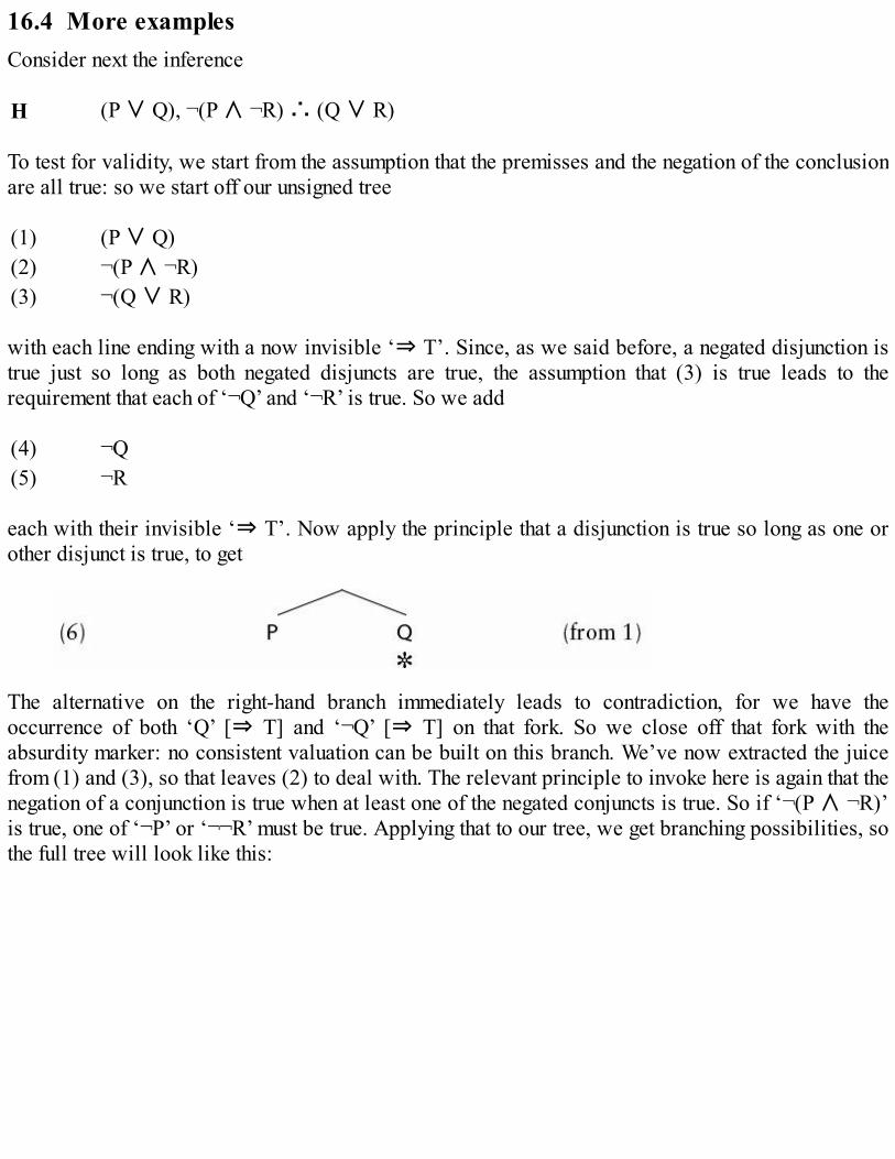
16.4 More examplesConsider next the inference

H (P ∨ Q), ¬(P ∧ ¬R) ∴ (Q ∨ R)

To test for validity, we start from the assumption that the premisses and the negation of the conclusionare all true: so we start off our unsigned tree

(1) (P ∨ Q)(2) ¬(P ∧ ¬R)(3) ¬(Q ∨ R)

with each line ending with a now invisible ‘⇒ T’. Since, as we said before, a negated disjunction istrue just so long as both negated disjuncts are true, the assumption that (3) is true leads to therequirement that each of ‘¬Q’ and ‘¬R’ is true. So we add

(4) ¬Q(5) ¬R

each with their invisible ‘⇒ T’. Now apply the principle that a disjunction is true so long as one orother disjunct is true, to get

The alternative on the right-hand branch immediately leads to contradiction, for we have theoccurrence of both ‘Q’ [⇒ T] and ‘¬Q’ [⇒ T] on that fork. So we close off that fork with theabsurdity marker: no consistent valuation can be built on this branch. We’ve now extracted the juicefrom (1) and (3), so that leaves (2) to deal with. The relevant principle to invoke here is again that thenegation of a conjunction is true when at least one of the negated conjuncts is true. So if ‘¬(P ∧ ¬R)’is true, one of ‘¬P’ or ‘¬¬R’ must be true. Applying that to our tree, we get branching possibilities, sothe full tree will look like this:

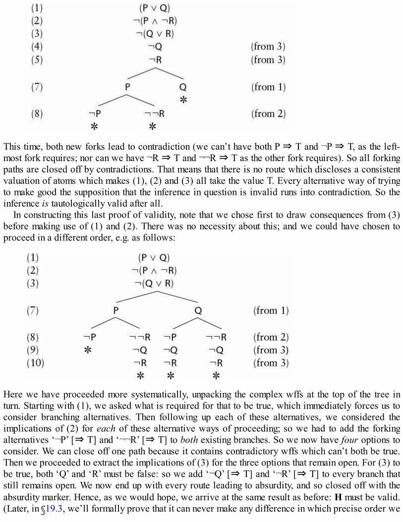
This time, both new forks lead to contradiction (we can’t have both P ⇒ T and ¬P ⇒ T, as the left-most fork requires; nor can we have ¬R ⇒ T and ¬¬R ⇒ T as the other fork requires). So all forkingpaths are closed off by contradictions. That means that there is no route which discloses a consistentvaluation of atoms which makes (1), (2) and (3) all take the value T. Every alternative way of tryingto make good the supposition that the inference in question is invalid runs into contradiction. So theinference is tautologically valid after all.

In constructing this last proof of validity, note that we chose first to draw consequences from (3)before making use of (1) and (2). There was no necessity about this; and we could have chosen toproceed in a different order, e.g. as follows:

Here we have proceeded more systematically, unpacking the complex wffs at the top of the tree inturn. Starting with (1), we asked what is required for that to be true, which immediately forces us toconsider branching alternatives. Then following up each of these alternatives, we considered theimplications of (2) for each of these alternative ways of proceeding; so we had to add the forkingalternatives ‘¬P’ [⇒ T] and ‘¬¬R’ [⇒ T] to both existing branches. So we now have four options toconsider. We can close off one path because it contains contradictory wffs which can’t both be true.Then we proceeded to extract the implications of (3) for the three options that remain open. For (3) tobe true, both ‘Q’ and ‘R’ must be false: so we add ‘¬Q’ [⇒ T] and ‘¬R’ [⇒ T] to every branch thatstill remains open. We now end up with every route leading to absurdity, and so closed off with theabsurdity marker. Hence, as we would hope, we arrive at the same result as before: H must be valid.(Later, in 19.3, we’ll formally prove that it can never make any difference in which precise order we

unpack wffs when ‘working backwards’.)Another example: what of the following inference?

I (P ∨ (Q ∧R)), (¬P ∨ R), ¬(Q ∨ ¬¬S) ∴ (S ∧ R)

We start off in the now familiar way, with the premisses and negated conclusion:

(1) (P ∨ (Q ∧R))(2) (¬P ∨ R)(3) ¬(Q ∨ ¬¬S)(4) ¬(S ∧ R)

A negated disjunction is true only if both disjuncts are false, i.e. the negated disjuncts are true. So (3)implies a couple of definite truth assignments

Where now? Well, we know that a pair of negation signs in effect cancel each other out. So we caninfer

Let’s now unpack the other complex wffs in turn. First we have

The right-hand branch doesn’t close off immediately, but if we have (Q ∧R) ⇒ T on that way ofmaking (1) true, then we must also have Q ⇒ T and R ⇒ T. So we can add to the right hand branchthus

And we’ve hit a contradiction between (5) and (9r) and can close off that branch. Proceeding downthe left-hand branch, we’ve so far ensured that (1) and (3) are true. To make (2) true we need either¬P ⇒ T or R ⇒ T. So we have

and the left-hand of the two branches we’ve added immediately closes off, since we can’t have ‘P’and ‘¬P’ both true. That leaves us with only (4) to unpack. So we apply the rule for negatedconjunctions again and the resulting tree from line (7) again looks like this:

So, all but one of the branches close. Looking at that remaining branch, however, and putting back thesuppressed assignments of truth, we can read off the following valuation

P ⇒ T, ¬Q ⇒ T (so Q ⇒ F), R ⇒ T, ¬S ⇒ T (so S ⇒ F).

This is designed to make the premisses of I true and the conclusion false (check that it does!). So theargument is tautologically invalid.

This tree technique is elegant and (usually) efficient. Our next task is to gather together the variousprinciples we have found for tree-building, check whether we need any others, and put them togetherin one systematic list. Though first, let’s briefly pause for breath.

16.5 SummaryTesting an argument for tautological validity is a matter of searching for ‘bad’ valuations. We cando this by a brute-force inspection of all possible valuations. Or we can ‘work backwards’, i.e.assume there is a bad valuation and try to determine what it would look like. If the suppositionthat there is such a bad valuation leads to contradiction, then the argument in question is valid.The ‘working backwards’ method, in the general case, will necessitate inspecting branchingalternative possibilities, e.g. looking at alternative ways of making a disjunction true. Theresulting working is naturally laid out in the form of a downward branching tree.By some simple tricks, we can ensure that every wff on such a tree is assigned the value T. Butthen, if every wff is assigned the same value, we needn’t bother to explicitly write down thevalue – giving us ‘unsigned’ trees.The official rules for tree-building follow in the next chapter.

Exercises 16Although we haven’t yet laid down formal rules, it is worth doing a bit of informal exploration to getmore feeling for the tree method before we dive into the official story. So, see how you get on testingthe following inferences for validity, using the techniques of this chapter. At this stage it might help tokeep writing down explicit ‘T’-only trees, appending ‘⇒ T’ alongside every wff to remind yourselfwhat you are doing and why you are doing it.

1. (R ∨ P), (R ∨ Q) ∴ (P ∨ Q)2. ¬(P ∧ ¬Q), P ∴ Q3. (¬P ∨ Q), (R ∨ P) ∴ (R ∧ Q)

4. ((P ∧ ¬Q) ∨ R), (Q ∨ S) ∴ (R ∧ S)5. P, ¬(P ∧ ¬Q), ¬(Q ∧ ¬R), (¬R ∨ S) ∴ S6. ((P ∧ Q) ∨ (R ∧ P)) ∴ ((Q ∨ R) ∨ P)

17

Rules for PL trees

This chapter gives a more formal description of the tree test for tautological validity. The firstsection, then, is necessarily going to be rather abstract. But it will really do no more than carefullyformulate the principles we’ve already used in the last chapter. (Those who get a bit fazed by this sortof abstraction can try skimming through the statement of the rules and the following illustrativesections a few times in quick succession, using each to throw light on the other.)

17.1 The official rulesAs we have seen, our ‘working backwards’ method of testing for tautological validity typicallyrequires us to explore alternatives. These explorations are most neatly set out in the form of trees(upside-down ones, with the ‘trunk’ at the top and the branches forking downwards). In fact, our treesare binary trees, meaning that a branch never forks more than two ways.

We’ll take the idea of a downward branching binary tree to be intuitively clear: we could getmathematically precise here, but little would be gained. The thing to emphasize is that trees fan outwithout branches being rejoined at a lower level: as in the case of a respectable family tree,incestuous reunions are banned.Some definitions will prove useful, though:

Positions on a tree are conventionally called nodes.Start from the topmost node of the tree, and and track down some route through the inverted treeto the bottom tip of a branch. The nodes en route form a path through the tree.In our truth-trees, the nodes are occupied by wffs. If a wff W occurs at a node on a path, we’llsay more briefly that W is on the path or that the path contains W.If a path contains a pair of wffs of the form W, ¬W, then the path is closed; otherwise it is open.If a tree has an open path it is open; otherwise the tree is closed.

And before we proceed, here’s a reminder of another definition:

A primitive wff is a wff which is either an atom or the negation of an atom ( 11.8). So a non-primitive wff is any wff that isn’t primitive (i.e. any complex wff that features more than asolitary negation sign).

Suppose, then, that we want to determine whether the premisses A1, A2, …, An tautologically entailthe conclusion C. We begin the truth-tree in the now familiar way by placing the Ai and ¬C at nodesdown the initial trunk of a tree (all accompanied by an invisible ‘⇒ T’). Then we try systematicallyto generate a ‘bad’ valuation that will indeed make these initial wffs all true.

The strategy at each stage is to infer, from the assumed truth of a non-primitive wff W already on

some path, shorter wffs which must also be true if that W is to be true (maybe we have to consideralternatives, so the path has to fork as we add them). When a path contains both a wff and its negation(both, of course, implicitly assigned the value T), then we know that this must be a contradictorydead-end and cannot lead to a consistent valuation of primitives. Such a path is closed, and we willmark off closed paths with the absurdity marker ‘ ’. We continue extending open paths by unpackingthe implications of non-primitive wffs on the path, with forks in the tree marking points where wehave alternatives to investigate. And we keep on going until either (i) all the paths we explore containcontradictory pairs of wffs and the tree is closed, or else (ii) we have no more wffs to unpack and weare still left with an open tree with at least one open path. (We’ll put that more carefully in a moment.)

What rules govern extending the tree at each stage? There are five, depending on the character ofthe non-primitive wff W we aim to unpack. The rules have already been illustrated informally in theprevious chapter, and are summed up in the box displayed opposite. Three quick comments:

The five rules exhaust all the cases of non-primitive wffs, as can be seen by quickly runningthrough the possibilities. Any wff is either an atom, or a conjunction (in which case apply rule(b)) or a disjunction (in which case apply rule (d)), or else the negation of something. In the lastcase, the wff must either be the negation of an atom, or of a conjunction (in which case applyrule (e)) or of a disjunction (in which case apply rule (c)), or finally it’s the negation of anegation (in which case apply rule (a)). So we have a rule to apply to every eventuality, until weget down to the level of primitives (atoms and negations of atoms).Why, in applying a rule to some wff W, must we add the appropriate (possibly alternative) wffsto the foot of every open path containing W? Because these different open paths containing W aresupposed to indicate alternative possible valuations where W is true – and we need to considerthe further implications of W’s truth for each of these alternative valuations.Note, these rules for unpacking wffs tell us what to do with a selected non-primitive W. But theydon’t tell us how to make the selection. Typically, the rules can be applied in various orders tothe same initial trunk of wffs. The chosen order won’t affect the ultimate verdict of the tree test.

Rules for unpacking wffs on PL trees

Suppose that W is a non-primitive wff on an open branch, which is supposed true on some valuation.One of the following cases must obtain:

(a) W is of the form ¬¬A. If W is true on a valuation, that means that A itself must be true: to unpackW, add A [⇒ T] to each open path through the tree containing W. Schematically,

(b) W is of the form (A ∧ B). If a conjunction W is true on a valuation, both its conjuncts must betrue: to unpack W, add both A [⇒ T] and B [⇒ T] to each open path containing W.Schematically,

(c) W is of the form ¬(A ∨ B). If the negation of a disjunction is true on a valuation, the disjunctionmust be false, and hence both its disjuncts false, and thus the negations of both disjuncts true. Soto unpack W, add ¬A [⇒ T] and ¬B [⇒ T] to each open path containing W. Schematically,

(d) W is of the form (A ∨ B). If W is true on a valuation, at least one of its disjuncts must be true.We have to explore alternatives. So to unpack W, add a new fork to each open path containing W,with branches leading to the alternatives A [⇒ T] and B [⇒ T]. Schematically,

(e) W is of the form ¬(A ∧ B). If W is true on a valuation, (A ∧ B) is false, and so at least one ofthe conjuncts must be false, i.e. at least one of their negations must be true. We have to explorealternatives. So to unpack W, add a new fork to each open path containing W, with branchesleading to the alternatives ¬A [⇒ T] and ¬B [⇒ T]. Schematically

Now, suppose that we have already applied the appropriate rule to some complex formula W. Thenit would be pointlessly redundant to apply the rule to the same W again. And it would be worse thanredundant to get ‘stuck in a loop’, repeatedly re-applying this same rule to W, time without end.Henceforth, then, we adopt the following structural rule for tree-construction:

When the appropriate rule has been fully applied to a non-primitive wff, we ‘check off’ the wff(with a ‘√’); and a wff, once checked off, can be thought of as ‘used up’, i.e. as no longeravailable to have one of the ‘unpacking’ rules applied to it.

This ensures that a properly constructed tree can’t go on for ever. Unpacking a wff generates shorterwffs: and since we are not allowed to revisit ‘used’ wffs, after a finite number of stages, we’ll run outof new wffs to check off, and there will be no more rules to apply.

So, with that ‘check off’ rule in play, here more carefully are step-by-step instructions for buildinga complete tree.

(1) Start off the trunk of the tree with the premisses A1, A2, …, An and the negation of conclusion C ofthe inference to be tested.

(2) Inspect any path which isn’t yet closed off by an absurdity marker to see whether it involves acontradiction, i.e. for some wff W it contains both W and also the corresponding formula ¬W. If itdoes, then we close that path with the marker, and ignore it henceforth.

(3) If there is no unchecked non-primitive formula W left on any open path, then stop!(4) Otherwise, we choose some unchecked non-primitive formula W that sits on an open path. We

then apply the appropriate rule from (a) to (e), and add the results to the foot of every open pathcontaining that W. We can then check off W.

(5) Loop back to step (2).

As just remarked, this tree-building procedure must eventually terminate. There are two possibleoutcomes. Either we end up with a closed tree, i.e. a tree such that every path through the tree closes(there is an absurdity marker at the foot of every branch). Or we end up with a completed open tree –i.e. one where some paths don’t close, and on each open path, we have repeatedly applied the rules(a) to (e) as much as we possibly can, so that every non-primitive formula on the path is used up andchecked off, but without always producing a contradiction.

Finally, here is the Basic Result about truth trees:

If, starting a tree with the wffs A1, A2, …, An, ¬C at the top, we can construct, using rules (a) to(e), a closed tree, then the argument from the premisses A1, A2, …, An to the conclusion C istautologically valid. Conversely, if applying the rules leads to some completed tree with an openbranch, then the argument in question is not tautologically valid.

We’ll prove the Basic Result in Chapter 19. But it should seem intuitively correct, since it onlyrestates the principle underlying all our worked examples in the previous chapter – namely, that if‘working backwards’ from the assumption that the premisses are true and the conclusion false landsus in self-contradic-tion, then that assumption can’t be made good and the given argument must bevalid after all; while if that assumption does lead to a consistent assignment of truth to variousprimitives, then the argument in question is invalid.

17.2 Tactics for treesA couple of pieces of tactical advice before we start working through more illustrative examples.

First, suppose that at a given point we have the option of applying either a ‘straight’ rule – i.e. oneof (a) to (c) – or one of the ‘branching’ rules (d) and (e). To take a very simple example, suppose wehave arrived at the following point on some branch of a tree:

How should we continue? Well, if we apply the ‘branching’ rule (d) first, and then rule (b), we willget

However, if we apply the rules in the reverse order, we get

This makes absolutely no difference in principle: either way we get a (sub)tree with two pathsthrough it, with exactly the same wffs occurring on the left path each time and exactly the same wffsoccurring on the right path each time. The only difference is that, in the case where we applied thebranching rule (d) first, we had to double the expenditure of ink when it came to applying rule (b),since we already had two branches to which to add ‘R’ and ‘S’. It is quicker and neater to proceed asin the second case. Moral: it generally pays to apply non-branching rules first when one has theoption.

The second bit of tactical advice is even more obvious: aim to close off branches as soon aspossible. If you have the option of applying a rule which will immediately lead to a path being closedoff, then it is good policy to select that option. Suppose, for example, that a tree begins

Then we have three options for applying the branching rule (d). If we blindly apply the rule to the firstwff first, and then deal with the others in turn, we get

Thus, after sprawling eight branches wide, most of the tree suddenly closes off, leaving us with justtwo open branches. One branch says that

¬R ⇒ T (so R ⇒ F), P ⇒ T, P′ ⇒ T and S ⇒ T

The other one yields

¬R ⇒ T (so R ⇒ F), Q ⇒ T, P′ ⇒ T and S ⇒ T

And either of those valuations will make the wffs on the trunk all true.But now suppose that we start again, and this time applying rule (d) to the premisses in the

opposite order. Then the completed tree looks like this:

We still end up with two open paths on the tree, carrying just the same wffs as before. But by ajudicious choice of the order of application for the branching rule, we have achieved a much moreneatly pruned structure. Evidently, it is sensible, wherever possible, to choose similarly to applyrules in an order which closes off branches as early as possible. A bit of practice enables you to spotgood choices!

(‘But hold on a moment! The first valuation just listed doesn’t explicitly assign any value to “Q”,

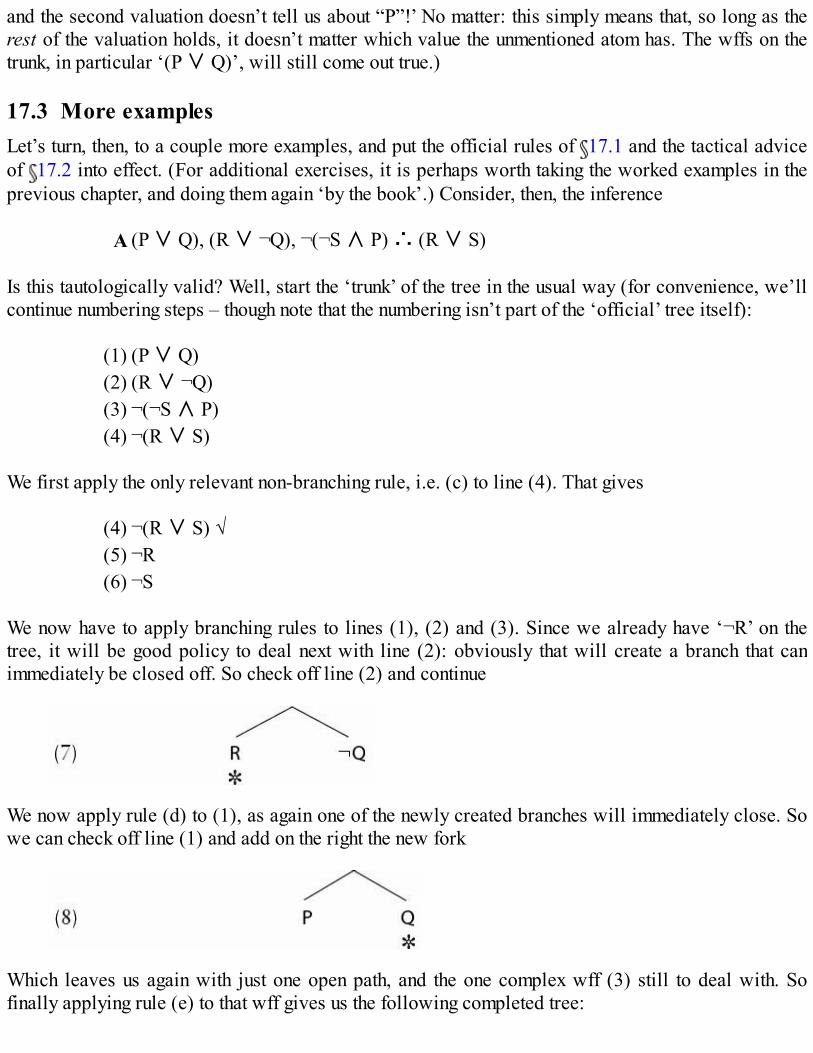
and the second valuation doesn’t tell us about “P”!’ No matter: this simply means that, so long as therest of the valuation holds, it doesn’t matter which value the unmentioned atom has. The wffs on thetrunk, in particular ‘(P ∨ Q)’, will still come out true.)

17.3 More examplesLet’s turn, then, to a couple more examples, and put the official rules of 17.1 and the tactical adviceof 17.2 into effect. (For additional exercises, it is perhaps worth taking the worked examples in theprevious chapter, and doing them again ‘by the book’.) Consider, then, the inference

A (P ∨ Q), (R ∨ ¬Q), ¬(¬S ∧ P) ∴ (R ∨ S)

Is this tautologically valid? Well, start the ‘trunk’ of the tree in the usual way (for convenience, we’llcontinue numbering steps – though note that the numbering isn’t part of the ‘official’ tree itself):

(1) (P ∨ Q)(2) (R ∨ ¬Q)(3) ¬(¬S ∧ P)(4) ¬(R ∨ S)

We first apply the only relevant non-branching rule, i.e. (c) to line (4). That gives

(4) ¬(R ∨ S) √(5) ¬R(6) ¬S

We now have to apply branching rules to lines (1), (2) and (3). Since we already have ‘¬R’ on thetree, it will be good policy to deal next with line (2): obviously that will create a branch that canimmediately be closed off. So check off line (2) and continue

We now apply rule (d) to (1), as again one of the newly created branches will immediately close. Sowe can check off line (1) and add on the right the new fork

Which leaves us again with just one open path, and the one complex wff (3) still to deal with. Sofinally applying rule (e) to that wff gives us the following completed tree:

Every downwards path closes off, showing that there is no consistent way of backtracking to avaluation of atoms which makes the premisses of the given argument true and the conclusion false.Hence A is valid.

Note carefully the application of rule (e) at the final step. The rule is: given a negated conjunction¬(A ∧ B) on an open path, add forks, with ¬A and ¬B on the two branches. Applied to (3), on the leftfork we need to add the negation of ‘¬S’, and that is ‘¬¬S’, not ‘S’. The application of (e), andlikewise (c), always results in the prefixing of a new negation sign. We can later use (a) to strip offpairs of negation signs if we need to: but this is a further step. In more advanced work, you willencounter logical systems with a non-classical understanding of negation. In particular, you’ll meetso-called intuitionistic logic (see 9.3), which lacks a rule like (a) and where ‘¬¬S’ is not equivalentto ‘S’. So it is bad to get into the habit of just ignoring double negations.

Another example. What are we to make of this inference?

B (P ∧ (Q ∨¬R)), ¬((P ∧ Q) ∧S)), (¬(P ∧ S) ∨R) ∴ ¬S

The truth-tree for this inference starts

NB again the doubling up of the negation signs at line (4). Let’s apply the non-branching rule (b) to(1), followed by the rule (e) to (2) to add

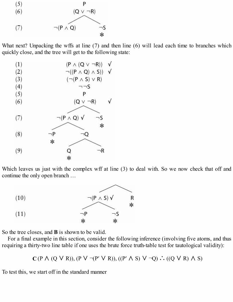
What next? Unpacking the wffs at line (7) and then line (6) will lead each time to branches whichquickly close, and the tree will get to the following state:

Which leaves us just with the complex wff at line (3) to deal with. So we now check that off andcontinue the only open branch …

So the tree closes, and B is shown to be valid.For a final example in this section, consider the following inference (involving five atoms, and thus

requiring a thirty-two line table if one uses the brute force truth-table test for tautological validity):

C (P ∧ (Q ∨ R)), (P ∨ ¬(P′ ∨ R)), ((P′ ∧ S) ∨ ¬Q) ∴ ((Q ∨ R) ∧ S)

To test this, we start off in the standard manner

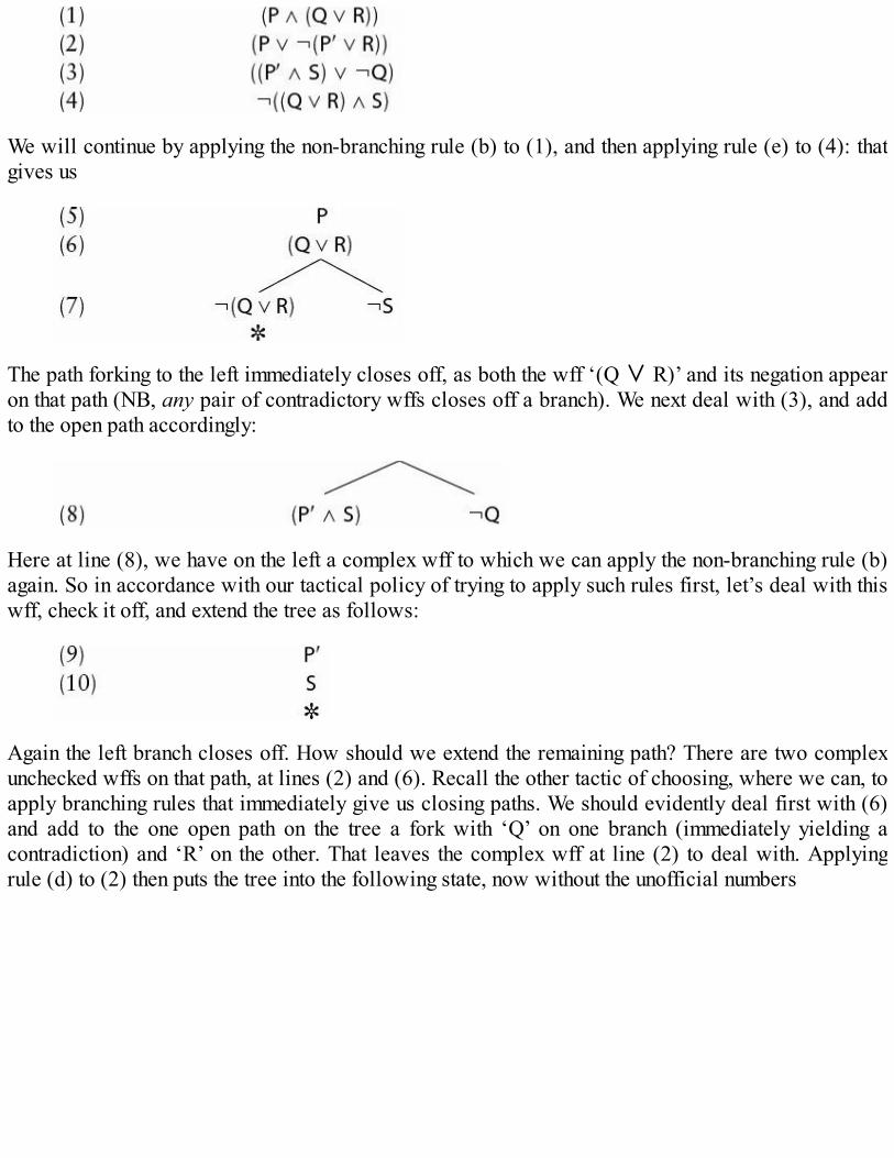
We will continue by applying the non-branching rule (b) to (1), and then applying rule (e) to (4): thatgives us

The path forking to the left immediately closes off, as both the wff ‘(Q ∨ R)’ and its negation appearon that path (NB, any pair of contradictory wffs closes off a branch). We next deal with (3), and addto the open path accordingly:

Here at line (8), we have on the left a complex wff to which we can apply the non-branching rule (b)again. So in accordance with our tactical policy of trying to apply such rules first, let’s deal with thiswff, check it off, and extend the tree as follows:

Again the left branch closes off. How should we extend the remaining path? There are two complexunchecked wffs on that path, at lines (2) and (6). Recall the other tactic of choosing, where we can, toapply branching rules that immediately give us closing paths. We should evidently deal first with (6)and add to the one open path on the tree a fork with ‘Q’ on one branch (immediately yielding acontradiction) and ‘R’ on the other. That leaves the complex wff at line (2) to deal with. Applyingrule (d) to (2) then puts the tree into the following state, now without the unofficial numbers

We are not quite done, since we have a new complex wff appearing on the right-hand branch at thelast line; so to finish the tree, we need to apply the relevant rule (c), and check off that complex wff asfollows:

Which at last does complete our tree: we now have ‘unpacked’ every complex wff featuring on openpaths, and we are still left at the end with an open pathway. From this branch, reading from the bottomup, we can read off the valuation P ⇒ T, R ⇒ T, ¬Q ⇒ T (so Q ⇒ F) and ¬S ⇒ T (so S ⇒ F). Thevalue of ‘P′’ is left undetermined, which means that the other values should suffice to fix the initialwffs on the trunk as true, no matter what value ‘P′’ has. And our valuation indeed verifies (1) to (4),as is easily checked. So C is invalid.

17.4 Testing for tautologiesThe tree test determines whether C has to be true, given the premisses Ai. As a special case, we canuse the test to determine whether C is a tautology, i.e. has to be true, period. We just suppose ¬C istrue, and then see if we can work backwards to extract a ‘bad’ valuation which will have thisconsequence. If we can, then C isn’t a tautology; if we can’t, then it is.

To take a fairly simple example, is

D ((P ∧ (Q ∨ R)) ∨ (¬P ∧ (¬Q ∧ ¬R)))

a tautology? Well, suppose it isn’t. Suppose that there is a valuation which makes

(1) ¬((P ∧ (Q ∨ R)) ∨ (¬P ∧ (¬Q ∧ ¬R)))

true. Unpacking (1) and making the next few tree-building moves we get

We now need to apply rule (e) to (3), and place the result (remember!) at the foot of each of the twoopen paths it heads. So we get

We have three marked paths that are evidently not going to close. But strictly speaking we are notquite finished yet. There are still non-primitive wffs on each of those paths, and we need to apply rule(a) in each case to strip off the double negations. So continuing we get …

And now we are finished. We have a completed open tree, and so D is not a tautology. (Exercise:read off the open branches the ‘bad’ valuations which make D false.)

For a final worked example, consider the wff

E (¬(¬(P ∧ Q) ∧ ¬(P ∧ R)) ∨ ¬(P ∧ (Q ∨ R)))

Is this a tautology? Well, start the tree:

(1) ¬(¬(¬(P ∧ Q) ∧ ¬(P ∧ R)) ∨ ¬(P ∧ (Q ∨ R)))

What now? How do we read this slightly monstrous wff? Working from the inside, we can usedifferent styles of brackets to make the groupings clearer, thus

(1) ¬[¬{¬(P ∧ Q) ∧ ¬(P ∧ R)} ∨ ¬{P ∧ (Q ∨ R)}]

which reveals (1) to be of the form ¬[A ∨ B], with A = ¬{¬(P ∧ Q) ∧ ¬(P ∧ R)}, and B = ¬{P ∧(Q ∨ R)}. So we need to apply rule (c) to get

(2) ¬¬{¬(P ∧ Q) ∧ ¬(P ∧ R)}(3) ¬¬{P ∧ (Q ∨ R)}

Next we obviously apply rule (a) to get rid of those paired negation signs

(4) {¬(P ∧ Q) ∧ ¬(P ∧ R)}(5) {P ∧ (Q ∨ R)}

Both of these wffs are conjunctions so we can apply rule (b) twice to get

(6) ¬(P ∧ Q)(7) ¬(P ∧ R)(8) P(9) (Q ∨ R)

The wffs at lines (1) to (5) have now all been checked off and ‘unpacked’, so we need now onlyworry about the wffs (6) to (9). Dealing with (6) and (7) first, we get

Which will leave just one unchecked non-primitive wff to deal with, at line (9). So to finish the tree…

Thus all branches close off, and the wff E is a tautology (you are hereby invited to check this byrunning a direct truth-table test…!).

17.5 Comparative efficiencyOperating the tree test for tautological validity often involves choices: in which order do we applythe unpacking rules? But we could make it fully mechanical by laying down strict rules for choosingwhich wff to unpack next. That would give us two mechanical tests for validity, the original truthtable test ‘search forwards’ through all valuations, looking for a bad one, and the tree test ‘searchbackwards’, starting from the assumption that there is a ‘bad’ valuation. As we’ve seen, runningthe tree test on an argument is often much faster than running the truth table test. Sometimes the gain isstaggering. Return to the example we gave in 13.2: take the inference from the 50 premisses ‘¬P, ¬P′,¬P′′, ¬P′′′, …, ¬P′′...′’ to the conclusion ‘Q’. Even if we could write down a line a second, just setting

out the 251 line truth-table (before looking for a bad line) would take half a million years. Writingdown a truth tree at the same rate would take less than a minute (just write down the premisses, thenegation of the conclusion and – hey presto! – we’ve got a complete open tree and the test is done).

Is the tree-test always more efficient? No. In the worst case scenario, trees can sprawl horribly.Take the inference with 50 premisses ‘(P ∨ P′), (P′ ∨P′′), (P′′ ∨ P′′′), …’ and conclusion ‘Q’.Obviously it is invalid. But running a tree-test, at least as we’ve so far described it, leads to anexponentially sprawling tree. When we unpack the first premiss, the tree splits into two branches;when we unpack the second premiss, each branch splits into two again; unpack the third premiss andwe get eight branches. So by the end of the tree, it has exploded into 250 branches; and even if wecould construct one complete downward path per second, that would be another ludicrous task.

Now, you might think that we just need to add some more bells and whistles to the tree test. Afterall, we can instantly spot that the last inference is invalid: we immediately see that the valuationwhich makes all the ‘P’s true and ‘Q’ false will make the disjunctive premisses all true andconclusion false. And if we can instantly spot that, can’t we build our way of doing the trick(whatever that is) into an improved tree test to speed things up? To which the answer is, yes, we canadd a few more particular tricks that can deal with some special cases: but there is no general-purpose trick that is guaranteed to avoid exponential sprawl. Put it this way: given an inferencewith fifty-something atoms, then with truth-tables and truth trees alike, even augmented with short-cuttricks, in the worst case applying either test for tautological validity is a million-year task.

Is there some other mechanical test for tautological validity which does better? No. (Or at least, soeveryone believes: but the issue relates to a still unsolved problem in the foundations of the theory ofcomputation.)

17.6 SummaryWe have set out the formal rules for building PL truth-trees to test inferences for tautologicalvalidity. The rules consist of step-by-step instructions for building a tree, ‘unpacking’ morecomplex wffs into simpler ones as the tree grows, checking off wffs as we use them up, andclosing off any paths which contain contradictory pairs of wffs.The instructions for tree-building don’t determine a unique tree, since we are allowed to choosewhich non-primitive wff to ‘unpack’ when there is more than one candidate.But it doesn’t matter which choices you make: the test will always give the same verdict. If thetree closes, then the argument under test is tautologically valid; if it doesn’t, it isn’t. (A proof ofthat comes later, in Chapter 19.)We can make life easier for ourselves by a couple of obvious tactics for tree building: applynon-branching rules before branching ones, and when possible choose to apply rules that lead toa branch quickly closing.The tree test can be used in an obvious extension to determine whether a given wff is a tautology.Running a tree test is very often quicker than a truth-table test. But not always.

Exercises 17A Revisit Exercises 13A, and now use the tree test to determine which of the arguments listed there

are tautologically valid.

B Revisit Exercises 12 and now use the tree test to determine which of (2) to (6) are tautologies.

C And since practice makes perfect, use the tree test to determine which of the following are true.

1. ((P ∨ Q) ∧ (P ∨ R)) ((Q ∧ R) ∨P)2. ((P ∧ ¬(P′ ∧R)) ∨ S), (P′ ∨ S) (R ∧ S)3. P, ¬(Q ∧ (P′ ∨ R)), ¬(¬Q ∧ P), ((P′ ∧S) ∨ (R ∧ S)) S4. (¬(¬(P ∧ Q) ∨ ¬(P ∧ R)) ∨ ¬(P ∨ (Q ∧ R)))5. ((P ∧ Q) ∨ (R ∧ P)), ¬(¬S ∧ P), ¬(Q ∧ R) (Q ∧ S)

D How would the rules and principles of tree-building need to be re-written if we had stuck to usingsigned trees, where wffs are explicitly assigned T or F?

18

PLC trees

We now extend the use of the tree test to cover inferences involving the material conditional.

18.1 Rules for PLC treesSuppose we want to extend the tree test for tautological validity to cover arguments expressed inPLC. We need rules that tell us how to disassemble wffs whose main connectives are ‘⊃’ and ‘≡’.

A wff of the form (A ⊃ B), which has ‘⊃’ as its main connective, is equivalent to thecorresponding wff (¬A ∨ B). So if (A ⊃ B) appears on a tree (silently assumed to be true, ofcourse), then we should unpack it as we would unpack (¬A ∨ B). So we’ll need to add new forks,leading to the alternatives ¬A and B.

Query: looking at the truth-table, aren’t there three ways of making (A ⊃ B) true – namely the waywhich makes A, B true, the way which makes ¬A, B true and the way which makes ¬A, ¬B true. Sowhy don’t we split the tree three ways, adding those pairs of wffs to the respective branches? Reply:no reason other than aesthetics! We could construct trees like that; it would in the end come to exactlythe same (see Exercise 18B). It is just prettier to stick to two-way splits.

To continue: a wff of the form (A ⊃ B) is only false when A is true and B false. So if ¬(A ⊃ B)appears on a path – i.e. (A ⊃ B) is assumed to be false – then that requires A, ¬B to be true on thesame valuation.

A wff of the form (A ≡ B) is true in two cases, when A and B are both true, and when A and B areboth false. So we should unpack (A ≡ B) disjunctively, adding new forks with A, B on one branch and¬A, ¬B on the other.

Finally, a wff of the form ¬(A ≡ B) is also true in two cases, when A is true and B false, and when Ais false and B true. So we should also unpack ¬(A ≡ B) disjunctively, this time adding new forks withA, ¬B on one branch and ¬A, B on the other.

These rules are summed up in the following box in the style of 17.1. The general principles forbuilding trees and then reading off the results of the test remain (of course) exactly the same as before.And there is an extended Basic Result: a PLC argument is tautologically valid if and only if its treecloses.

Further rules for unpacking wffs on PLC trees

Suppose that W is a non-primitive wff on an open branch, which is supposed true on some valuation.Then, as well as the five cases (a) to (e) as listed before, there are now four further possibilities tocover:

(f) W is of the form (A ⊃ B). To unpack W, add a new fork to each open path containing W, withbranches leading to the alternatives ¬A [⇒ T] and B [⇒ T]. Schematically,

(g) W is of the form ¬(A ⊃ B). To unpack W, add both A [⇒ T] and ¬B [⇒ T] to each open pathcontaining W. Schematically,

(h) W is of the form (A ≡ B). To unpack W, add a new fork to each open path containing W, with A[⇒ T] and B [⇒ T], on one branch, and ¬A [⇒ T] and ¬B [⇒ T] on the other. Schematically,

(i) W is of the form ¬(A ≡ B). To unpack W, add a new fork to each open path containing W, with A[⇒ T] and ¬B [⇒ T], on one branch, and ¬A [⇒ T] and B [⇒ T] on the other. Schematically,

18.2 ExamplesWe’ll immediately turn to a few examples. First, let’s test the following argument which we’ve metbefore (interpret the atoms as you will):

A (P ⊃ Q), (Q ⊃ R) ∴ (P ⊃ R)

Here’s the corresponding completed tree, where we apply the non-branching rule (g) first, and omitthe unnecessary line numbers.

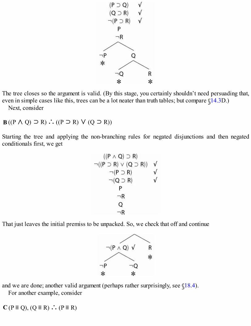
The tree closes so the argument is valid. (By this stage, you certainly shouldn’t need persuading that,even in simple cases like this, trees can be a lot neater than truth tables; but compare 14.3D.)

Next, consider

B ((P ∧ Q) ⊃ R) ∴ ((P ⊃ R) ∨ (Q ⊃ R))

Starting the tree and applying the non-branching rules for negated disjunctions and then negatedconditionals first, we get

That just leaves the initial premiss to be unpacked. So, we check that off and continue

and we are done; another valid argument (perhaps rather surprisingly, see 18.4).For another example, consider

C (P ≡ Q), (Q ≡ R) ∴ (P ≡ R)

This time the tree starts

and there are no non-branching rules to apply. So let’s just proceed by unpacking wffs from the topdown, remembering to add the necessary new forks at each stage to every open branch:

Again the tree closes and the argument is confirmed to be valid (make sure you follow exactly howthis tree has been constructed).

Next, we’ll test whether the following is a tautology:

D ((P ⊃ Q) ∨ (Q ⊃ P))

As before ( 17.4), to use a tree test we start with the negation of this wff and aim to findcontradictions. The negated disjunction unpacks into the negated disjuncts, and then we apply rule (g)a couple of times to get

so D comes out as a tautology. Perhaps that’s another surprising result, and we’ll again comment on itin 18.4.

What about the following?

E ({P ⊃ Q} ⊃ {(Q ≡ R) ⊃(P ⊃ R)})

A moment’s reflection suggests that this ought to be a tautology (why?); and indeed it is. Starting withthe negation of E and applying non-branching rules first we get

and now we apply the branching rules to the unchecked wffs to finish the tree

18.3 An invitation to be lazyNow for a slightly more complex example, which incidentally also illustrates a general point abouttrees (whether PL or PLC trees). Consider

F (P ⊃ (Q ⊃ R)), (S ⊃ (Q ∨ P)) ∴ (S ⊃ R)

The tree starts

So far, we’ve applied the non-branching rule to the negated conclusion first, and then the twobranching rules to the premisses (choosing first the application that immediately leads to a closedbranch). And now let’s pause here, though the tree isn’t completed yet, for neither of thoseoccurrences of ‘(Q ⊃ R)’ has been checked off.

Note, however, that the path up from the bottom left node is completed: i.e. there are no uncheckedwffs left on that path through the tree. Further work on the tree therefore can’t close off that path.Hence argument F is already shown to be tautologically invalid. For an argument to be validaccording to the tree test, all paths through the tree must close; that means that just one completedopen path is enough to show invalidity. In other words, an unfinished tree with a completed open pathdemonstrates invalidity. (Compare: for an argument to be valid according to the truth-table test, alllines of the truth table must be ‘good’. But one bad line is enough to show invalidity.)

Reading up that open branch, we find the primitives ¬P, Q, ¬R, S all silently assigned the valuetrue. So one valuation which makes the premisses true and conclusion false is P ⇒ F, Q ⇒ T, R ⇒ F,S ⇒ T. Completing the other two currently open branches will in fact reveal another valuation whichhas the same effect. But if you are feeling lazy, you can leave the tree unfinished.

For a final worked example, consider the argument

G ((¬Q ⊃ R) ⊃(Q ≡ S)), (P ∧ R), ¬(Q ∧ S) ∴ ¬((P ∧ Q) ⊃ (R ∧ S))

We can begin a tree thus:

So far, so obvious (let’s hope!). Now unpack the shorter of the two remaining unchecked wffs, and wehave to add the two forks

There are still three open branches. So now let’s take the remaining unchecked wff, apply rule (e),and continue the left-most branch.

The other two branches will get similar continuations, but again we’ll be lazy, as we’ve alreadyfound a completed open branch. As before, there is little point in filling out the rest of the tree, asfurther growth on the other branches won’t affect this open branch. The tree is not going to close, andthat settles that G too is tautologically invalid.

18.4 More translational issuesGiven the meaning of ‘⊃’, the results of the last two sections are entirely unproblematic. But acouple look a bit puzzling when we translate them back into English, using the vernacular ‘if …, then…’. We aren’t going to reopen all the debates of Chapter 15, but we shouldn’t just pass by withoutcomment.

(1) An example due to Richard Jeffrey. Consider again the inference

B ((P ∧ Q) ⊃ R) ∴ ((P ⊃ R) ∨ (Q ⊃ R))

We’ve shown this to be tautologically valid. Now consider the following, got by reading ‘P’ as thecaptain turns his key, ‘Q’ as the gunnery officer turns his key, and ‘R’ as the missile fires, andrendering the horseshoe connective by ‘if’.

If the captain turns his key and the gunnery officer turns his key, then the missile fires. Henceeither the missile fires if the captain turns his key, or else it fires if the gunnery officer turns hiskey.

That surely can’t be a valid inference, or there would be no dual-key fail-safe systems! What’s gonewrong? (Question for consideration: are the conditionals here, despite being ‘indicative’ in surfacegrammatical form, naturally read as possible-world conditionals? That is to say, we treat theconditionals as telling us what would happen if a key were turned, even if no key is turned in theactual world – which is why they are not truth-functional.)

(2) The conditional ‘If it is boiling hot, then it is freezing cold’ looks simply absurd; so does theconditional ‘If it is freezing cold, then it is boiling hot’. So consider the disjunction

Either it is freezing cold if it is boiling hot or it is boiling hot if it is freezing cold.

This looks to be disjunction of silly falsehoods; so it should be false. Put ‘P’ as it is freezing cold,‘Q’ as it is boiling hot, render ‘if’ by ‘⊃’, and we get

D ((P ⊃ Q) ∨ (Q ⊃ P))

which, far from being false, we’ve just shown is a tautology. Isn’t that quite unacceptable? (Questionfor consideration: when we take e.g. ‘If it is boiling hot, then it is freezing cold’ as plainly false arewe again reading it as a possible-world conditional?)

(3) I can’t resist adding another example, also due to Richard Jeffrey. Note that the inference

H ((P ⊃ Q) ⊃ R), ¬P ∴ R

is also tautologically valid (check that with a quick tree test!). But interpret ‘P’ as we advance, ‘Q’ asthe enemy retreats and ‘R’ as the enemy lose. Then this corresponds to the argument

If the enemy retreats if we advance, then they lose. But we won’t advance. So the enemy lose!

which is surely not valid. (You can’t zap the enemy with inaction plus mere logic. Question forconsideration: are the conditionals here really possible world conditionals yet again?)

And so it goes! There are numerous cases where, on the face of it, PLC arguments involving‘⊃’which are tautologically valid (and hence plain valid) become, at first blush, problematic anddubious when translated back into English using ‘if …, then …’. Maybe, with greater or lesser

difficulty, the problematic appearances can often be explained away. But the moral needs repeating:Treat the material conditional with great care.

18.5 SummaryThe tree-building rules we met in Chapter 16 can be simply extended to tell us how to unpackwffs whose main connectives are ‘⊃’ and ‘≡’.We have also noted that we can stop work on a tree once a complete open branch is found (i.e.an open branch with no unchecked non-primitives remaining). One completed open branch isenough to show than the argument being tested is invalid.

Exercises 18

A Redo Exercises 14B using the tree method to determine which of the arguments are tautologicallyvalid.

B (a) Suppose we added to our rules for tree-building the following: you can at any point extend anopen branch with a fork of the form

Show informally that this change would make no difference (in the sense that a tree which closesusing the original rules will still close, and a tree which stays open using the original rules willremain open).(b) Show that we could therefore replace our rule for unpacking conditionals with this morecomplex one:

(c) Conclude that we could therefore replace our rule for unpacking conditionals with thefollowing three-ply rule ( 18.1):

19

PL trees vindicated

The tree method appears to be a very elegant way of determining tautological validity. But now weought to confirm what we’ve been taking for granted, namely that the tree test gets things right (wecalled that the ‘Basic Result’ about trees). So the business of this short chapter is to vindicate the treetest. It can be skipped by those who have no taste for such ‘metalogical’ niceties!

19.1 The tree method is soundThe Basic Result ( 17.1) has two parts. The first half says:

(S)If, starting a tree with the wffs A1, A2, A3, …, An, ¬C at the top, we can construct a closedtree by following the official rules for tree building, then the inference from the premissesAi to conclusion C is indeed tautologically valid.

Equivalently: if an inference is invalid, then a corresponding tree can’t close.Let’s (re)establish a bit of terminology, before turning to the proof of (S). A set of wffs is

satisfiable if there is a valuation of the relevant atoms which makes all the wffs in the set true.Derivatively, we will call a path through a tree satisfiable if there is a valuation (of the relevantatoms that appear in wffs on the path) which makes all the wffs on the path true.

It is immediate that a satisfiable path through a tree cannot close. For a closed path by definitioncontains a contradictory pair of wffs, W and ¬W; and no valuation can make such a pair true together.And that observation underlies the following …

Proof of (S) Suppose that there is some valuation which ensures that

A1 ⇒ T, A2 ⇒ T, A3 ⇒ T, … , An ⇒ T, ¬C ⇒ T

and hence that the initial ‘trunk’ of the corresponding truth-tree is satisfiable (so the inference inquestion is invalid). Now consider what happens as we extend our tree, step by step, applying theofficial rules. At each stage, a satisfiable path will get extended to a longer satisfiable path.

That’s obvious with the non-branching rules: for example, if there is a valuation which makeseverything on a path true, including a wff (A ∧ B), then when we apply rule (b) to extend that pathby adding A and B, the same valuation will obviously make both these added new wffs true as well– since if the conjunction is true on a valuation, so are the conjuncts. So the extended path willremain satisfiable. You can easily check that the same is true for extensions by means of rules (a)and (c) – and for (g) as well, on those occasions when ‘⊃’ is also in play ( 18.1).

And in a case where we extend a satisfiable path by using a branching rule, one branch (atleast) of the extended tree must still remain satisfiable. For instance, if there is a valuation which

makes everything on a path true, including a wff (A ∨B), then when we apply rule (d) to extendthis path with A on one fork and B on the other, the same valuation must make at least one of thesenew wffs true. For if a disjunction is true on a valuation, so is one its disjuncts. Hence, at a fork wecan always choose at least one extension of a satisfiable path which remains satisfiable. And youcan easily check that the same is true for extensions by means of rule (e), and likewise for thebranching rules (f), (h) and (i) governing (bi)conditionals.

Thus, if we start with a satisfiable trunk, then however far down we extend the tree according toour rules, there will always remain at least one satisfiable path through it. But as we noted, asatisfiable path must stay open. Hence a tree with a satisfiable trunk can never fully close.

So, if a tree does close, then its trunk isn’t satisfiable. There is no valuation which makes true allthe premisses and the negation of the conclusion of the inference under test, and hence thatinference is valid. QED.

In summary: the tree method is indeed a reliable or sound one (a PL or PLC argument which theappropriate tree test says is tautologically valid really is tautologically valid).

19.2 The tree method is completeThe other half of the Basic Result says:

(C)If, starting a tree with the wffs A1, A2, A3, ..., An, ¬C at the top, we can construct acomplete open tree by following the official rules for tree building, then the inferencefrom the premisses Ai to conclusion C is tautologically invalid.

To prove this result, it is enough to prove two subsidiary results, as follows.

(C1)For any completed open path, there is a valuation which makes the primitives true(for the idea of a ‘primitive’ see 17.1).

(C2)If there’s a valuation for the atoms that appear in the wffs on a completed open pathwhich makes the primitives true, then it will make all the wffs on the path true.

For suppose (C1) and (C2) are correct. By definition, if a tree headed by the Ai and ¬C is open, then ithas at least one completed open path through it. By (C1), there’s a valuation which satisfies theprimitives on that path; hence by (C2) there’s a valuation which satisfies all the wffs on that path,including the wffs on the initial trunk. That valuation therefore makes all of Ai and ¬C true. So, as (C)claims, the inference from the premisses Ai to conclusion C must be tautologically invalid.

Hence we now just need to prove (C1) and (C2):

Proof of (C1) Take a completed open path. Climb up it from the bottom, and construct the followingvaluation for the atoms which occur in the wffs on the branch:

When you encounter a totally bare atom on the path, assign it the value T; any other atoms, thatappear only inside some non-atomic wff on the path, get the value F.

Call this the chosen valuation.

An example: suppose that as you climb up the chosen path you encounter in sequence the wffs

Q, ¬P, (¬P ∧ Q), R, (R∨S), ((R ∨ S) ∨ P), ((¬P ∧ Q) ∨S)

then the chosen valuation constructed as we march up the branch is

Q ⇒ T, P ⇒ F, R ⇒ T, S ⇒F

By construction, the chosen valuation makes all the primitives on the given path true. For aprimitive is either (i) a bare atom, or (ii) the negation of an atom. Case (i): the valuation triviallymakes the bare atoms true, because that’s how it was chosen! Case (ii): suppose the negation of anatom, say ‘¬P’, appears on the path. Since by hypothesis the path is open and contains nocontradictions, the corresponding bare atom ‘P’ can’t appear on the path. So the chosen valuationwill make ‘P’ false: and hence the primitive wff ‘¬P’ that does appear on the branch will, asrequired, be true. QED

We’ll now gives two proofs of (C2): first a brisk official proof, and then a more relaxed, intuitiveone.

Official proof of (C2) Take a completed open path, and suppose the primitives on this path are alltrue on some valuation, but also that this valuation makes one or more other wffs on the path false.Choose one of the shortest of these false wffs. Since the primitives are all true by hypothesis, thisshortest false wff is non-primitive. And since the path is a completed one, this wff must have beenchecked off, and had the corresponding rule applied to it. Now consider cases. Suppose theshortest false wff is of the form (A ∧ B); then both A and B must appear on the path, and beingshorter must by assumption be true. But that’s impossible: we can’t have (A ∧ B) false yet A and Beach true. Again, suppose the shortest false wff is of the form (A ∨ B); then either A or B mustappear on the chosen path, and being shorter must by hypothesis be true. But that’s impossible: wecan’t have (A ∨ B) false yet one of its disjuncts true. The other cases are similar. Hence the ideathat there are false wffs on the path, and hence shortest false wffs, leads to contradiction. Thus thechosen valuation which makes the primitives true makes every wff on the chosen path true. QED.

That argument is brisk, but perhaps it doesn’t really bring out why (C2) holds. So here is …

A more intuitive proof of (C2)? We’ll say that the wffs S1, S2, … are together truth-makers for W ifthe joint truth of S1, S2 … would ensure that W is true. For example, the wffs A, B are truth-makers for(A ∧ B); the wff ¬A by itself is a truth-maker for ¬(A ∧ B). And so on.

Take another look at the tree-building rules. They say, for example, that if W is of the form (A ∧B) we add its truth-makers A and B to its path; while if W is of the form ¬(A ∧ B) we split the path,adding the truth-maker ¬A to one fork, and the alternative truth-maker ¬B to the other. Likewise forthe other rules. Each rule enjoins us to extend a path (maybe forking) by adding appropriate truth-makers for non-primitive wffs.

Now, by the definition of a completed path, every non-primitive wff has been checked off and‘unpacked’ by the appropriate rule. So that means a completed open path set must contain truth-makers for every non-primitive wff (and if those truth-makers are non-primitive, there will befurther truth-makers for them, until we get down the shortest possible wffs).

Suppose, then, that we can find a valuation which does indeed make true the shortest wffs on thepath, i.e. it makes the primitives true. Then, truth will spread upwards. As we work back up thepath, the truth of the shortest wffs (the truth-makers for the next shortest wffs) will make those nextshortest wffs true, and then the next shortest, and so on up. So everything will be made true so longas we make the primitives true. QED.

So that establishes (C1) and (C2) and hence (C).(C) says, in effect, that we have enough rules for tree-building. Suppose we were allowed to use

only three of the rules instead of all five/nine. If a tree built using just these three rules closed, thatwould still indicate a valid argument. But the fact that a tree didn’t close would not mean that theargument is invalid: it might stay open because we didn’t have enough rules for dealing with (say)disjunctions. But (C) shows we have a complete set of tree-building rules; there are enough rules toestablish that any tautologically valid PL/PLC inference is indeed valid.

19.3 A corollary and a further resultFirst, we’ll quickly note a corollary of the Basic Result: as announced in 16.4, the order in which thetree-building rules are applied (when we have a choice) can’t matter. Why?

Well, note that the Basic Result entails that if an argument is tautologically valid, then any properlybuilt tree will close, irrespective of the order in which we apply the relevant tree-building rules.Likewise, if an argument is invalid, any appropriate tree will stay open, again irrespective of theorder in which tree-building rules are applied.

Secondly, let’s note a result which slightly extends our argument for (C). Let’s say that a set Σ ofPL wffs is saturated if the following conditions obtain:

(a) if a wff of the form ¬¬A is in Σ, then so is A;(b) if a wff of the form (A ∧ B) is in Σ, then so are both A and B;(c) if a wff of the form ¬(A ∨ B) is in Σ, then so are both ¬A and ¬B;(d) if a wff of the form (A ∨ B) is in Σ, then so is at least one of A and B;(e) if a wff of the form ¬(A ∧ B) is in Σ, then so is at least one of ¬A and ¬B.

Likewise a set of PLC wffs Σ is saturated if it satisfies (a) to (e) plus the conditions

(f) if a wff of the form (A ⊃ B) is in Σ, then so is at least one of ¬A and B;(g) if a wff of the form ¬(A ⊃ B) is in Σ, then so are both A and ¬B;(h) if a wff of the form (A≡B) is in Σ, then so are either both A and B or both ¬A and ¬B;(i) if a wff of the form ¬(A≡B) is in Σ, then so are either both A and ¬B or both ¬A and B.

(Why ‘saturated’? Because such a set is saturated with truth-makers, containing a truth-maker forevery non-primitive wff in it.)

We’ll also say that Σ is syntactically consistent if it contains no pairs of wffs of the form A, ¬A.(Compare the semantic definition of logical consistency in 2.1.)

The conditions (a) to (i) will have an entirely familiar look. They correspond exactly to the rulesfor building up a path on a PL (PLC) tree; so it is immediate that the wffs on a completed open pathform a syntactically consistent saturated set. The set will be consistent, since an open path contains nocontradictions, and saturated because checking off every non-primitive wff on the path in order to

complete the tree ensures that (a) to (i) are fulfilled on the path. So our earlier result that a completedopen path is satisfiable is just a version of the rather more general result that every syntacticallyconsistent saturated set Σ of PL (PLC) wffs is satisfiable – i.e. there is a valuation which makes allthe wffs in Σ true.

The proof of this result goes exactly as before. First, we define the chosen valuation for Σ: if theatom A appears naked in Σ, assign it the value T; otherwise assign that atom the value F. It is simple toshow – as in (C1) – that this chosen valuation makes all the primitives in Σ true, and then – as in (C2)– that a valuation which makes all the primitives in Σ true will make every wff in Σ true.

The advantage of talking about ‘consistent saturated sets of wffs’ as opposed to ‘sets of wffs on acompleted open branch of a tree’ is that it emphasizes that the arrangement of wffs onto a tree isn’t ofthe essence here. It’s the structure described by (a) to (i) above that ensures that the set, if consistent,is satisfiable.

And, if we abstract from the case where the wffs are to be written out on a common-or-gardenfinite tree, then we can even allow the case where the consistent saturated set Σ contains infinitelymany wffs. The proof that consistent saturated sets are satisfiable doesn’t depend on any assumptionof finitude. Of course, in the case of propositional logic, the consideration of infinite sets of wffs ismostly of ‘technical’ interest. But matters are different, as we will see in Chapter 30, when we turn tothinking about more complex logical systems.

19.4 SummaryWe have shown that the tree test is sound: i.e. if an argument is judged valid by the test – i.e. theappropriate tree closes – then it is indeed tautologically valid.We have shown that the tree test is complete: i.e. if an argument is tautologically valid, then thetree test will reveal it as such by the appropriate tree closing. Equivalently, if an appropriatetree stays open, the argument under test is invalid.The proof of these results shows that it doesn’t matter in which order we apply the tree-buildingrules (when we have a choice).

Exercises 19A Show how to extend the following sets of wffs into consistent saturated sets (hint: think of the

given sets as ‘trunks’ of trees; you want to extend the trunks to some compete open path).

1. ¬Q, (P ⊃ Q), (¬¬R ⊃ (P ∧ R))2. ¬(Q ∧ (P′ ∨ R)), ¬(¬Q ∧ P), ((P′ ∧S) ∨ (R ∧ S))3. (Q ⊃ (P ∨ R)), ¬(P ⊃ S), ((P ∨S) ∧ (¬Q ⊃ S)), ((S ∨ R) ⊃ ¬P)

In each case, what is the ‘chosen valuation’ for the set? Check that it does indeed make true all thewffs in the set.

B Rewrite the arguments (C1) and (C2) to turn them into explicit arguments for the thesis that everysyntactically consistent saturated set Σ of PL (PLC) wffs is satisfiable. Confirm that thesearguments don’t depend on whether Σ is finite.

20

Trees and proofs

The unsigned trees that we have been exploring were introduced as shorthand for signed trees, a wayof setting out arguments in English about PL inferences. But, as we will now explain, we can alsothink of them as proofs in PL.

20.1 Choices, choices …Outside the logic classroom, when we want to convince ourselves that an inference is valid, we don’tuse techniques like the truth-table test. As we pointed out way back in Chapter 5, we usually seekproofs: i.e. we try to show that the desired conclusion follows from the premisses by chainingtogether a sequence of obviously acceptable steps into a multi-step argument.

Suppose, then, that we want to develop ways of warranting PL inferences by means of proof-reasoning inside PL. How should we proceed? (By the way, take talk of ‘PL’ in this chapter to coverPLC as well.)

It is very important to stress that there is no single ‘right’ way of setting out proofs. Indeed, in thisbook we have already touched on no less than three different ways of setting out multi-steparguments.

(1)In Chapter 5, we introduced proofs set out linearly, one step below another (though wealso added an indentation device to signal when suppositions were being madetemporarily, for the sake of argument).

(2)

Then in Chapter 8 (see 8.2), we noted that some linear arguments can very naturally berearranged into tree structures, with the initial assumptions appearing at the tips ofbranches, and the branches joining as we bring together propositions to derive aconsequence. We work down the tree until we are left with the final conclusion of theproof at the bottom of the trunk. (Our examples happened to feature arguments inaugmented English about which strings of PL symbols are wffs.)

(3)

In Chapters 16–18, we found that some other arguments are naturally set out as invertedtrees. We start with some assumptions at the top of the tree, and work down trying to findcontradictions, splitting branches at various choice points as we descend the downwards-branching tree. (Our examples were again arguments in augmented English, but this timearguments about the tautological validity of PL inferences.

Which way of regimenting arguments in (augmented) English should we follow if we want to build aproof system for warranting inferences inside PL?

The headline answer is this: if our primary aim is to develop ways of arguing in PL that echo thenatural contours of ordinary-language arguments, then the first model is the one to emulate. For more

advanced technical work, the second model has a lot going for it. But for ease of manipulation bybeginners, downwards-branching trees are the thing.

20.2 Trees as arguments in PLTo develop that last point, note next that we in fact don’t have to do any new work to get a system forbuilding tree arguments in PL. For our unsigned downwards-branching trees can already bethought of as arguments in PL.

Of course, that is not how we introduced them. Given a PL inference

A (P ∧ R), ¬(P ∧Q) ∴ ¬Q

we set about warranting it by supposing there is a valuation which makes the premisses and negationof the conclusion false, and then trying to show that that supposition leads to contradiction(s). That’sall metalinguistic reasoning. Here’s a corresponding tree in full-dress form, quotation marks and all:

Now, we later got into the habit of writing trees in unsigned form for brevity’s sake, dropping thequotation marks and then the explicit assignment of truth:

But, at least as originally introduced, a pruned tree like this still abbreviates a way of arguingmetalinguistically, i.e. a way of arguing in English about whether there is a possible valuation whichmakes the premisses of the PL inference true and conclusion false.

However – and here’s the new suggestion – we can equally well look at the pruned tree anotherway. It can also be regarded as a multi-step argument framed purely in PL terms (recall that we

quietly announced at the very outset, 8.1, that ‘✼’ belongs to the alphabet of PL, so all the symbolson the tree really do belong to that language). Imagine again wanting to defend the inference A, butthis time without straying into meta-linguistic reasoning. We take the premisses ‘(P ∧ R)’, ‘¬(P ∧Q)’and the negated conclusion ‘¬¬Q’ as suppositions. Then we argue step-by-step, first to ‘P’ and ‘R’,then to ‘Q’, and then on, via the alternatives ‘¬P’ and ‘¬Q’, to absurdities. Our tree argument revealsthat our initial supposition leads to unavoidable contradiction. So that warrants the inference A isvalid (compare 13.8(i)).

The point generalizes. We can systematically re-read our originally meta-linguistic truth-trees asbeing arguments in PL, arguments that aim to reveal inconsistencies. If the tree headed A1, A2, …, An,¬C closes, i.e. ends up in contradictions, take that as an object-language argument warranting theinference A1, A2, …, An ∴ C.

20.3 More natural deductions?Still, it might very reasonably be said, this is certainly not the most natural way of building argumentsin PL.

Consider this very simple vernacular argument:

BPopper and Russell both wrote on political philosophy. It isn’t the case that bothPopper and Quine wrote on political philosophy. So Quine didn’t write on politicalphilosophy.

That is obviously valid. But if you need to convince yourself that it is valid, here’s a natural line ofargument, rather laboriously set out in the style of 5.4:

Now let’s render this natural reasoning into PL, using ‘P’ for ‘Popper wrote on political philosophy’,etc. The inference B gets translated as ‘(P ∧ R), ¬(P ∧Q) ∴ ¬Q’, i.e. as A again. And we mightreplicate the natural line of reasoning B′ in PL along the following lines (the numbering and Englishside-commentary isn’t part of the argument proper).

Let’s compare this ‘natural deduction’ in PL with the tree proof A″ warranting the same inference.One obvious difference is that B″, like most real-life arguments, ends with the desired conclusion.

To be sure, there is a passage of indirect argumentation en route, as we make a temporary suppositionfor the sake of argument: but the overall argument takes us ultimately to the desired conclusion. An A″-type tree however always starts by assuming the negation of the conclusion along with thepremisses, and unpicks the implications of that.

But that’s perhaps not the fundamental difference. Thinking about B″ more, note that at line (4) wemove from the premiss ‘(P ∧ R)’ to the interim conclusion ‘P’. This takes us from a more complex toa simpler wff by (so to speak) eliminating the connective ‘∧’ according to the rule ‘∧-Elimination’:

(∧E) From a wff of the form (A ∧ B) we can infer A, and equally we can infer B.

But then at line (5) we move from the two previous steps, ‘P’ and ‘Q’ to their conjunction ‘(P ∧ Q)’.Another perfectly valid inference of course! This time, however, we move from a pair of simplerwffs to a more complex one by introducing the connective ‘∧’ into a wff according to the rule

(∧I) From the wffs A, B we can infer their conjunction (A ∧ B).

This is typical of most proof systems. They have (in a phrase) both elimination and introductionrules for using connectives in inferences.

And now contrast the tree-building rules invoked in tree proofs ( 17.1). These rules always take usfrom more complex to simpler wffs. For example, if a conjunction like ‘(P ∧ Q)’ is already on apath, we add its conjuncts; but we never move in the opposite direction (never take a pair ofconjuncts and add the conjunction to the tree). Our tree-building rules are all ‘elimination’ rules.

The two noted differences between ‘natural deductions’ and tree proofs are of course intimatelyrelated. If we want to be able to argue directly to conclusions, and conclusions can themselves becomplex, we’ll typically need to be able to build up complex wffs by introducing connectives: sowe’ll need introduction rules.

However, once we have introduction rules available, proof-building can be trickier than in anelimination-rules-only system. Imagine, for example, that we’d started the proof B″ in the same waybut then got struck in a groove, applying and reapplying the rule (∧I):

These inferences are all perfectly valid, but take us further and further away from our desiredconclusion. They are, no doubt, daft inference moves to make, given we are trying to prove ‘¬Q’. Butthat’s the point: having introduction rules may well allow us to generate more ‘natural’ proofs, but italso allows us to drift off into cascades of irrelevancies. By contrast, systems of tree proofs (whichonly have elimination rules) put very much tighter constraints on what we can do at any point inbuilding a proof.

There’s no right choice here. It’s a trade-off between ‘naturalness’ and ease of proof-building. Forexperience suggests that trees are easier for beginners (after all, we’ve already pretty painlesslyslipped into using them). Less thought is required to get a tree proof to work. This is already so forsimple propositional logic: but is emphatically the case when we turn to the logic of quantifiers.

Which all goes to explain our choice of a less ‘natural’ proof-style in this book. (This way, we canstill convey the general idea of a formal proof-system, without having to spend too much time talkingabout strategies for proof-discovery in natural deduction systems.)

20.4 What rules for trees?So we’ll say no more about ‘natural deduction’ proofs (whether linear proofs like B″ or rearrangedinto downward-joining trees as in 8.2). But even if we fix on downward-branching trees as ourproof-structure of choice, that doesn’t fully determine which rules of proof-building we should adoptfor truth-functional logic. In 17.1 we fixed on one set of rules to adopt, but it isn’t unique.

The basic rule for tree-building is: extend an open branch by adding to it further wffs which mustalso be true assuming that wffs already on the branch are true (splitting the tree into two brancheswhen we have to consider alternatives).

Given that basic principle, we could adopt – for example – the following rules for dealing withnegated disjunctions and negated conjunctions. Schematically,

These new rules are legitimate because each tells us to add to the tree a wff which must be true if thegiven wff is true. In fact, we could replace our original rules (c) and (e) with these two new rules.For note, when combined with the existing rules (b) and (d) for unpacking conjunctions anddisjunctions, our new rules yield

which, in two steps, give us back the effects of our original one-step rules.That kind of possible variation in choice of rules is obviously pretty trivial. Here is a more

significant variation. For any C, (C ∨ ¬C) is always true on any valuation of its atoms. Hence addinga wff of that form to a branch would conform to the general principle that we can extend branches byadding further wffs which are true on the valuation which makes the initial wffs true. So we couldintroduce the rule that we can at any point extend a branch by adding an instance of the law ofexcluded middle ( 12.1; see also Exercise 18B). As you’d expect this makes no difference at all towhat we can prove using trees. A major cost of adding such a rule is that it introduces into our treesystem the possibility of getting lost adding irrelevancies. But intriguingly, having this additional ruleavailable can also speed up proofs radically (at least, that’s true when we extend trees to coverquantifier logic, in the style of Chapters 25 onwards). George Boolos has given a pretty example ofan inference which can be proved valid in a few pages when this new rule is available, and for which‘the smallest closed tree contains more symbols that there are nanoseconds between Big Bangs’ whenit isn’t! So if we particularly care about maximizing the number of proofs which are feasible (can bedone in a sensible amount of time) we’ll add the suggested new rule – and if we don’t, then we won’t.

These last remarks, like the discussion of the previous section, again drive home the point thatthere is no single ‘right’ proof system for truth-functional propositional logic. Which type of systemwe prefer to use, and which rules we adopt within that type of system, is a matter of how we weighttheir various virtues and shortcomings. Don’t be fazed when you discover that different logic textsmake different choices.

20.5 and , soundness and completenessThis is as good a place as any to introduce another bit of standard symbolism which you could wellencounter elsewhere. Suppose we pick on some preferred style of proof layout, and some set of rulesof inference for propositional logic. Call that proof system S. If there is some array of wffs whichcounts as a proof in S with premisses A1, A2, …, An and conclusion C, we write A1, A2, …, An S C.

Compare: ‘ ’ is a metalinguistic symbol, added to English (in 13.7) for abbreviatory purposes, toexpress the semantic relation that holds between some premisses and a conclusion when there is novaluation which makes the former all true and the latter false. ‘ S’ is also a metalinguistic symbol,added to English for abbreviatory purposes, this time to express the syntactic relation that holdswhen we can construct a suitable proof in system S. This is a syntactic relation because whether anarray of wffs counts as a proof doesn’t depend on their meaning, but only on whether the wffs arerelated in the ways allowed by the formal proof-building rules of S. (The use of the single turnstilefor the syntactic proof relation and the double turnstile for the semantic entailment relation is anabsolutely standard notational convention: learn it. If context makes it clear what proof-system S is inquestion, the subscript can be dropped.)

Obviously, for any proof system worth its keep, we want the following to hold for any Ai and C:

(S) If A1, A2, …, An S C then A1, A2, …, An C.

Suppose that didn’t hold. Then we could have a ‘proof’ in S that C followed from the Ai when in factC isn’t entailed by the premisses. The proof system wouldn’t be reliable, or sound (to use the usualterm).

We’d also like the following:

(C) If A1, A2, …, An C then A1, A2, …, An S C.

In other words, what we’d like is that, whenever the Ai taken together do in fact entail C, then there isa proof in S which reflects that. We’d like our proof system to be adequate to the task of warrantingall the tautologically valid inferences, or to be complete (again to use the standard term). There are alarge number of variant proof systems for propositional logic on the market which are, as we want,sound and complete.

Returning from generalities to the particular case of tree proofs: let’s now write A1, A2, …, An T Cwhen there is a closed PL/PLC tree headed by A1, A2, …, An, ¬C. Then we indeed have soundnessand completeness, i.e.

(SC) A1, A2, …, An T C if and only if A1, A2, …, An C.

For that just neatly sums up what we proved in Chapter 19.

20.6 SummaryPL trees were introduced as (shorthand for) metalinguistic arguments about truth-valuations ofPL wffs. But closed trees can easily be reinterpreted as object-language proofs (proofs of theinconsistency of the set of wffs A1, A2, …, An, ¬C, thus warranting the inference A1, A2, …, An ∴C).Tree proofs are not the most natural proofs, but are perhaps most easily managed by beginners.Different proof systems have different pros and cons: there is no ‘right’ system for truth-functional logic.

Interlude

After propositional logic

In the last seven chapters:

We have argued that the material conditional is the only candidate for translating ordinarylanguage conditionals by a truth-function, and we have discussed how good (or bad) atranslation this is.We found it convenient, though not strictly necessary, to add a special symbol to PL to expressthe material conditional, giving us the extended language PLC.We introduced truth-trees as a ‘fast track’ way of determining whether a PL or PLC inference istautologically valid.We showed that the tree method does indeed work as advertised (i.e. a correctly constructed treecloses if and only if the argument being tested is valid).Finally, we saw how to reconstrue trees (originally introduced as regimenting metalinguisticreasoning about PL/PLC wffs) as proofs in PL/PLC.

But put together with what has gone before – now making some twenty chapters and nearly twohundred pages in total – this still hasn’t taken us beyond elementary propositional logic.

Which, you might very well think, is really rather too much of a good thing. And, true enough, ourcareful extended treatment of propositional logic is none too exciting in itself. However, our mainreason for dwelling on it is that it does now give us a very secure basis from which to move on totackle something much more substantial, namely predicate logic (or first-order quantificationtheory, to use a more technical label).

This theory deals with the logic of inferences involving quantifiers such as ‘all’ and ‘some’ and‘no’ as well as the connectives. It’s arguable that this, together with the logic of identity, in effectcovers all the deductive reasoning that we need in mathematics and science. But whether or not thatbold thesis is right, it is undeniable that quantificational logic is very rich and powerful.

We’ll adopt the same two-stage strategy we used in tackling propositional logic. So we design asuitable formal language QL for expressing quantified propositions; then we look at how to assessarguments when framed in QL.

We’ll find that, while the syntax and semantics of PL/PLC was very straightforward, the designof the language QL, with its quantifier/variable notation, requires more sophistication.We can define a notion of q-validity for QL inferences, which is a sort of generalization of theidea of tautological validity for PL/PLC inferences.But there is no prospect of being able to mechanically test for q-validity in the way that we canmechanically test for tautologically validity (in fact, we can prove that there is no mechanicaltest for q-validity).

That means that when warranting QL inferences, proof methods really come into their own.We’ll build a proof system on the basis of the now familiar tree proofs for propositional logic. Itis a relatively easy extension.

Our first task, then, is to motivate the quantifier/variable notation on which QL is built.

21

Quantifiers

In this chapter, we reflect on some of the vagaries of quantifiers in ordinary English. We find somepointers for the design of an artificial language suitable for exploring the logic of quantifiers.

21.1 Quantifiers in argumentsIn Chapters 7 to 20, we were concerned with a very limited class of inferences, those whose validityor invalidity turns solely upon the way that the premisses and conclusion are built up using thepropositional connectives. So we didn’t need to discern any internal structure below the level ofwhole sentential clauses. We are now going to consider inferences whose validity (or lack of it) doesdepend on a finer level of structure. Take for example:

Fido is a cat.All cats are scary.So, Fido is scary.

The Baron hates anyone who loves Alma.Fritz loves Alma.So, the Baron hates Fritz.

Some philosophers admire every logician.No philosopher admires any charlatan.So, no logician is a charlatan.

These three arguments are all clearly valid, and equally clearly their validity is not a matter of thedistribution of propositional connectives (because they don’t contain any such connectives!). If weexposed no more than the way that whole sentential clauses are related by any propositionalconnectives, then these arguments could only be assigned the unrevealing and utterly unreliableinferential form A, B, so C. We therefore need to dig deeper.

What is crucial for these arguments is the occurrence of quantifying expressions such as ‘all’,‘anyone’, ‘some’, ‘every’, ‘no’, which are used to form complex terms like ‘all men’, ‘somephilosophers’ etc. Our target is to understand the logic of such arguments.

21.2 Quantifiers in ordinary languageEnglish expressions of generality behave in tediously complex ways. For example, consider thefollowing as stand-alone claims:

(1) Every play by Shakespeare is worth seeing.

(2) Any play by Shakespeare is worth seeing.

They express the same universal generalization about all the plays. But compare the way the samesentences embed in wider contexts:

(4) I don’t believe that every play by Shakespeare is worth seeing.(5) I don’t believe that any play by Shakespeare is worth seeing.(6) If every play by Shakespeare is worth seeing, I’ll eat my hat.(7) If any play by Shakespeare is worth seeing, I’ll eat my hat.

The messages expressed in each pair are quite different: so ‘every’ and ‘any’ sentences are notgenerally equivalent.

Next, consider:

(8) All plays by Shakespeare are worth seeing.(9) Each play by Shakespeare is worth seeing.

These also say, it seems, just the same as (1) and (2). And compare, e.g.

(10) I don’t believe that all plays by Shakespeare are worth seeing.(11) If all plays by Shakespeare are worth seeing, I’ll eat my hat.

(10) is equivalent to (4), and (11) to (6). So sentences containing ‘all’ typically behave on embeddinglike sentences with ‘every’ rather than ‘any’. Likewise for ‘each’ sentences (though they don’t seem toembed quite so naturally). So can at least we say that ‘all’, ‘each’ and ‘every’ constructions are juststylistic variants?

Well, here too there are complications. Not every occurrence of ‘all’ can be simply replaced by‘every’ or ‘each’: consider ‘All fresh snow is white’. And some ‘all’ propositions seem naturally totake the reading ‘all, considered as totality’, while a corresponding ‘each’ proposition takes thereading ‘each, considered separately’. For example, compare:

(12) Jack can read all of the plays in a day.(13) Jack can read each of the plays in a day.

(12) reports a feat of speed-reading; (13) makes Jack sound a bit slow.So, given that we are interested in the basic logic of arguments involving generalizations, but are

not especially interested in theorizing about the complexities of English usage, it seems veryattractive to pursue the strategy of constructing an artificial language with just one, simply-behaved,way of forming universal generalizations. Similarly for some other quantifiers. Then, as withpropositional logic, we can tackle the assessment of quantificational inferences in two stages. First,we translate the argument into our artificial language, treating the quantifiers in a uniform and tidyway; and then we assess the translated argument for validity.

21.3 Quantifiers and scope

There’s another reason for pursuing this strategy of building an artificial language, in addition towanting to side-step the multiple varieties of English usage. For English expressions of generality arebeset by scope ambiguities (for introductory remarks on scope ambiguity, see 7.2 and 9.6, wherewe first encountered the notion in connection with structurally ambiguous sentences of the kind A or Band C).

To work up to an example, consider the following pair of sentences:

(1) Some Republican senators smoked dope in the nineteen sixties.(2) Some women died from illegal abortions in the nineteen sixties.

As a shock headline in the newspaper, (1) is naturally read as saying, of some present Republicansenators, that they have a dark secret in their past (namely that they dabbled in illegal drugs in thesixties). But (2) is not to be read, ludicrously, as saying of some present women that they have asecret in their past (namely that they died of an illegal abortion back in the sixties). The claim is ofcourse that some women then existing died from illegal abortions. A natural way of describing thesituation is to say that we treat the tense operator ‘in the sixties’ as having a different scope in the twosentences. In the first case we take the tense operator to modify only the verb phrase ‘smoked dope’,while in the second case it is the whole proposition ‘some women died of illegal abortions’ which is(so to speak) to be evaluated with respect to the sixties. With a bit of grammatical butchery of tenses,and adding brackets for maximal clarity, we might thus represent the natural readings of the twosentences as follows:

(1′) (Some Republican senators are such that)(in the sixties it was true that) they smoke dope.(2′) (In the sixties it was true that)(some women are such that) they die from illegal abortions.

Here the final verbs are now deemed to be tenseless, and the order of operators shows the relativescopes of the tense operator and the quantifier, i.e. shows how much of the sentence concerns the past.

Consider, however, the following sentence:

(3) Some senior Republican senators plotted against the party leadership in 1988.

This seems simply ambiguous: are we saying that some of the then Republican senators plotted, orrather that some of the current lot plotted when they were young turks? We could be saying either

(3′) (In 1988 it was true that)(some senior Republican senators are such that) they plot;

or else

(3″) (Some senior Republican senators are such that)(in 1988 it was true that) they plot.

Both readings are fairly naturally available, so the original sentence is ambiguous. And the ambiguityis plausibly diagnosed as a scope ambiguity. The issue is: which has wider scope, which governsmore of the sentence, the tense operator or the quantifier?

Mixing expressions of generality and tense operators is prone to produce scope ambiguities. Sotoo is mixing quantifiers with modal operators (i.e. with expressions of necessity and possibility).

Consider, for example, the philosophical claim

(4) All sensory experiences are possibly delusory.

Does this mean that each and every sensory experience is one which, taken separately, is open todoubt, i.e.

(4′) (Every sensory experience is such that)(it is possible that) it is delusory?

Or is the thought that the whole lot could be delusory all at once, i.e.

(4″) (It is possible that)(every sensory experience is such that) it is delusory?

These claims are certainly different, and it is evidently philosophically important which reading ismeant e.g. in arguments for scepticism about the senses. For even if (4′) is true, (4″) doesn’t follow.Compare

(5) Every competitor might possibly win,

and its two readings:

(5′) (Every competitor is such that)(it is possible that) he wins.

(5″) (It is possible that)(every competitor is such that) he wins = (It is possible that) everycompetitor wins.

It could be that (5′) is true because the tournament is fairly run and the competitors well matched,while (5″) is false because it is a knock-out tournament with rules ensuring that only one ultimatewinner will emerge.

However, modal logic and the logic of tense operators are both beyond the scope of this book. So,to come to the kinds of case that do immediately concern us, let’s consider next what happens whenwe mix expressions of generality with negation.

We’ll take just one kind of example. Usually, a statement of the kind ‘Some Fs are not Gs’ is heardas entirely compatible with ‘Some Fs are Gs’. For example, ‘Some students are not logic enthusiasts’is no doubt sadly true; but it is compatible with the happier truth ‘Some students are logicenthusiasts’. But now consider the following case. Jack says ‘Some footballers deserve to earn fivemillion a year’. Jill, in response, takes a high moral tone, expostulates about the evils of huge wagesin a world of such poverty and deprivation, and concludes: ‘So some footballers damned well do notdeserve to earn five million a year’. Jill certainly doesn’t intend to be heard as saying somethingcompatible with Jack’s original remark! Thus, though vernacular English sentences of the form ‘SomeFs are not Gs’ are usually construed as meaning

(6′) (Some Fs are such that)(it is not the case that) they are Gs,

in some contexts the negation can be understood to have wide scope, i.e. to govern the wholesentence, with the resulting message being:

(6″) (It is not the case that)(some Fs are such that) they are Gs.

As in the tensed and modal cases, then, there is a potential for scope ambiguity when we mixquantifiers with negation – though context, emphasis, and plausibility considerations very often serveto privilege one reading and prevent misunderstanding.

Finally, let’s consider what can happen when a sentence contains more than one quantifier.Suppose you discover each of these is true:

(7) Jack is besotted with some film star;(7′) James is besotted with some film star;(7″) Jeremy is besotted with some film star.

Here you have found a property shared by each of Jack, James and Jeremy, namely the property ofbeing bewitched by some star or other (not necessarily the same one in each case). You might betempted to generalize from that sample to the rest of the logic class, and arrive at the ratherdepressing speculation that

(8) Every man in the class is besotted with some film star,

meaning that every man is like Jack, James and Jeremy in being enthralled by some star or other.Now a rather different scenario. This time you wonder whether any of these are true:

(9) Every man in the class is besotted with Cameron Diaz,(9′) Every man in the class is besotted with Gwyneth Paltrow,(9″) Every man in the class is besotted with Jennifer Lopez.

Here you have predicated the same property of each of Cameron Diaz, Gwyneth Paltrow and JenniferLopez, i.e. the property of being warmly admired by all men in the logic class. Now perhaps each ofthese predications turns out to be false (there is an exceptional man in each case). You might thenretreat to the less specific speculation that perhaps

(10) Every man in the class is besotted with some film star

meaning that there is some star who is admired by every man in the group. Here we have the samedoubly quantified sentence again as (8), but in the new context it conveys a different message. Forthere is all the difference between saying that everyone admires someone or other and saying thatsomeone is admired by everyone (just as there is all the difference between saying that every roadleads somewhere or other, and saying that there is somewhere where every road leads: compare 4.4). So the ordinary English sentence ‘Every man in the class is besotted with some film star’ ispotentially ambiguous between two readings:

(10′) (Every man in the class is such that)(there is some film star such that) he is besottedwith her.

(10″) (There is some film star such that)(every man in the class is such that) he is besotted

with her.

Again, therefore, we have a potential scope ambiguity, this time when we get certain doublyquantified sentences. Though again we should not exaggerate the problem; context and perhaps adefault preference for the first reading normally serve to remove this ambiguity in practice.

Note that these four kinds of scope ambiguity, where quantifiers are mixed with tense, modality andnegation and other quantifiers, do not occur when proper names are used instead of the quantifierexpressions. Consider:

(3°) John Doe plotted in 1988.(5°) Kasparov might possibly win.(6°) Michael does not deserve five million a year.(10°) Jack is besotted with Gwyneth Paltrow.

Those are all quite unambiguous. As it is sometimes put, genuine names are scopeless; whereas withquantifiers issues of relative scope can arise.

So all this points to a key design requirement on an artificial language apt for use when we areexploring the logic of generality. We must devise our notation so that the scope of a quantifier isalways clear and there is no possibility of scope ambiguities. And this means building in at groundlevel some way of marking the contrast between quantifiers and scopeless names.

21.4 Expressing quantification unambiguouslyHow then shall we express generality in a formal language? Well, consider again the linguistic devicewhich we slipped into using above, i.e. the device of using quantifier operators like ‘Every man in theclass is such that’, ‘Some Republican senator is such that’, …. These quantifier operators areprefixed to sentential forms constructed with pronouns, such as ‘he wins’, ‘he plotted’, ‘he is besottedwith her’, and so forth. The order of the quantifier operators with respect to other quantifiers andnegation (or other operators like tenses and modalities) then gives their relative scope according tothe obvious rule operators apply only to what follows them. This very natural device enables us toexpress ourselves very clearly and without ambiguity, even if at the expense of a little prolixity. Sowhy not use the very same device in a formal language?

There is just one wrinkle: suppose we want to express the thought that everyone loves someone orother using prefixed quantifiers. Then it won’t quite do to write

(1) (Everyone is such that)(there is someone such that) he/she loves him/her.

For that just introduces a new ambiguity. Which quantifiers are the pronouns respectively tied to? Isit, so to speak, everyone or someone who is doing the loving? But it is easy to rephrase: todisambiguate we just need something like

(2) (Everyone is such that)(there is someone such that) the former loves the latter,

which is plainly to be distinguished from

(3) (Everyone is such that)(there is someone is such that) the latter loves the former.

The expressions ‘the former’, ‘the latter’ function as pronouns linked to particular quantifiers. If wewere dealing with more than two quantifiers, we could instead use ‘the first’, ‘the second’, ‘thethird’, as in (say)

(4) (Every integer is such that)(every integer is such that)(there is some integer such that)the third is the product of the first and second,

which says that multiplying any two integers yields an integer.Using pronouns like ‘former/latter’ or ‘the first/second/third’ in a formal context, however, would

have considerable drawbacks. For when manipulating complex sentences with many quantifiers, whatcounts as ‘the first’ or ‘the second’ etc. will keep changing. So here’s a neat alternative trick,borrowed from the mathematicians. We introduce some new pronouns ‘x’, ‘y’, ‘z’ …; and then wetag our quantifier prefixes with these new pronouns in order to signal which quantifier goes withwhich pronoun. Then we can say ‘For any integers x and y there’s an integer z such that z is theproduct of x and y’. Or more stiltedly, we can put it like this:

(4′) (Every integer x is such that)(every integer y is such that)(there is some integer z suchthat) z is the product of x and y.

This use of ‘x’, ‘y’ and ‘z’ of course comes very naturally in this mathematical example: but thesame notation could be readily adopted for use much more widely, so that we write, e.g.

(2′) (Everyone x is such that)(someone y is such that) x loves y.(3′) (Someone x is such that)(everyone y is such that) y loves x.

There is nothing mysterious about the use of the so-called individual variables ‘x’ and ‘y’ here: theyare simply a snappier replacement for everyday pronouns.

Now for a bit of mere abbreviation. Instead of ‘every x is such that’, we could use simply thenotation ‘∀x’, with the rotated ‘A’ reminding us that this is also the all operator. And instead of‘there is some y such that’ let’s simply use ‘∃y’, with the rotated ‘E’ reminding us of another way ofexpressing that quantifier, namely ‘there exists some y such that’. Then, at least given a context whereit is clear that what is in question are people, our last two examples can be abbreviated very briskly,as

(2″) (∀x)(∃y)x loves y,(3″) (∃x)(∀y)x loves y.

Given a different context where it is clear that what is in question are integers, we can equally crisplywrite our arithmetical proposition

(4″) (∀x)(∀y)(∃z)(z is the product of x and y).

Now, so far, all this could still be treated as just so much augmented, abbreviated English. But, inessence, it exemplifies the notation for generality we will be adopting in QL, a version of thestandard logicians’ language for encoding quantificational arguments. We will use variablescorresponding to ‘x’, ‘y’, ‘z’ to do the work of pronouns, and use prefixed quantifiers on the model of‘∀x’, ‘∃y’ to do the work of ‘Every x is such that’ and ‘Some y is such that’. And that, apart from afew bells and whistles, will give us all we need.

In sum, the design of QL is guided by one very simple and compelling insight, namely thatpropositions involving quantifiers can be unambiguously expressed by using prefixed quantifieroperators applied to core clauses involving pronouns. Once that basic idea has been understood, therest really is plain sailing!

21.5 SummaryOrdinary English expressions of generality behave in complex ways (con-sider the availabilityof ‘all’, ‘every’, ‘any’, and ‘each’ to express universal generalizations, and compare thebehaviour of these quantifiers in complex contexts). And sentences involving such quantifiersare prone to scope ambiguities.So (following the ‘divide and rule’ strategy introduced in 7.3) we want to devise a formalartificial language QL that avoids the complexities and scope ambiguities of English. Our guidewill be a rather heavy handed and prolix apparatus already available in English, i.e. the use ofprefixed quantifiers operators of the kind ‘everyone is such that’, ‘someone is such that’, whichcan be used to express messages unambiguously.So, QL will be supplied with quantifiers like ‘∀x’, ‘∃y’, etc. which operate in a similar way,along with variables like ‘x’, ‘y’, etc. to act as corresponding pronouns.

22

QL introduced

In the last chapter we introduced the idea of the quantifier/variable notation for expressing generalpropositions. This chapter gives a relaxed, informal sketch of the formal language QL whichincorporates that idea.

22.1 Names and predicatesWe want, for a start, to be able to formalize arguments like ‘Fido is a cat; all cats are scary; so, Fidois scary’. We are going to use a quantifier/variable notation for expressing the second, general,premiss. But as a preliminary step, we first need to adopt a standard mode of expressing andrevealing the structure of non-general propositions such as the first premiss, ‘Fido is a cat’. Wetherefore need, as basic ingredients of QL, a stock of names and predicates.

Since we won’t be digging any deeper than the name/predicate/quantifier structure of sentences, thenames and predicates in QL might as well be as simple as possible, i.e. single letters. Hence, for thenames (or as we officially call them, individual constants) let’s for a start use

m, n, o, …

(i.e. lower case letters, not from the end of the alphabet).A predicate comes with a number of slots waiting to be filled up with names (or pronouns, etc.) to

form sentences. Thus compare the one-place English predicates ‘… smokes’, ‘… is a philosopher’;the two-place predicates ‘… is besotted with …’, ‘… was a pupil of …’; the three-place predicate‘… prefers … to …’, ‘… is between … and …’; and so forth. We will similarly supply QL with

one place predicates: F, G, H, …two place predicates: L, M, …three place predicates: R, S, …

and so on (all upper case letters).Then the rule for constructing the most basic sort of sentence of QL is simply that an n-place

predicate combines with n names (not necessarily different ones) to form an atomic wff. And just as amatter of convention (of no deep significance at all) we form that combination by writing thepredicate followed by the right number of names. Thus

Fn, Lnm, Loo, Rnmo, Romo

are sample atomic wffs.Of course, when we come to present the official syntax of QL, we’ll need to be more precise, and

not just give open-ended lists of the expressions which are to count as names/constants and

predicates. We’ll then also add to the class of atomic wffs. But in this chapter we will continue togive an incomplete and informal presentation (diving into the full-dress official story straight awaywould introduce distracting complications).

So much, then, for some unofficial syntax for atomic wffs. As for the informal interpretation of ouratomic wffs, that is equally straightforward. We fix on some code-book or interpretation for QL, forinstance the one where

‘m’ means Socrates‘n’ means Plato‘o’ means Aristotle‘F’ means … is wise‘L’ means … loves …‘R’ means … prefers … to …

Then the atoms above will, of course, get the following interpretation:

‘Fn’ means Plato is wise.‘Lnm’ means Plato loves Socrates.‘Loo’ means Aristotle loves himself.‘Rnmo’ means Plato prefers Socrates to Aristotle.‘Romo’ means Aristotle prefers Socrates to himself.

Note, the order in which names occur when combined with a predicate matters in QL just as it doesin English.

22.2 Connectives in QLQL has two ways of building up more complex expressions from simpler ones. The application ofquantifiers is one. But first, we will just take over from PLC our five propositional connectives(including ‘⊃’ and ‘≡’, and keeping the familiar bracketing conventions). The result of applying theseconnectives to a wff or pair of wffs of QL again yields another wff. So the following are wffs:

(Fm ∨Fn)¬(Lnm ∧ Lmn)(Rnmo ⊃(Lnm ∧¬Lno))((Fm ∨Fn)≡ (Lom ∨ Lon))

The meaning of the connectives remains as before. (Simple exercise: translate these, interpreting thenames and predicates as in the previous section.)

The only point to emphasize here is that the connectives added to QL remain essentiallypropositional connectives, i.e. they continue to combine proposition-like clauses. So we musttranslate

Plato and Aristotle are wise

as

(Fn ∧Fo)

and not as

F(n ∧o)

A propositional connective cannot connect constants; hence ‘(n ∧o)’ is simply ill-formed. Similarly,to translate

Plato is wise and handsome

we need something like

(Fn ∧Gn)

and not

(F ∧G)n

which is also ill-formed; a propositional connective can’t connect QL predicates.

22.3 Adding the quantifiersWe are following the design plan of 21.4, so we need to add to our language a stock of pronouns,more often called individual variables:

x, y, z, …

(i.e. lower case letters from the end of the alphabet). We also need a couple of symbols to use informing quantifiers

∀, ∃.

Either of those symbols followed by an individual variable yields a quantifier. Thus

∀x, ∀y, ∀z, …

are universal quantifiers meaning, roughly, ‘everyone/everything x is such that’, etc. We can alsoread them, more snappily, as ‘for all x’, ‘for all y’, etc. Likewise,

∃x, ∃y, ∃z, …

are existential quantifiers meaning, roughly, ‘someone/something x is such that’, etc. We can readthem, more snappily, as ‘for some x’, ‘for some y’, etc.

By the way, in our informal remarks before ( 21.4), we used bracketing round quantifiers: wewrote, e.g., ‘(∀x)(∃y)x loves y’. Such brackets aren’t needed, though many logic books do retainthem. We will henceforth opt for the more modern, bracket-free, notation. You will have no trouble atall reading the bracketed version if you are familiar with our austere version. (Though note that someolder books use simply ‘(x)’ instead of ‘(∀x)’.)

In the end, we want to construct complete quantified sentences, without pronouns dangling free (i.e.without pronouns that aren’t tied to associated quantifiers). So a natural first rule for building up QLwffs introduces quantifiers and variables together. The rule is: Take a wff with one or more

occurrences of some constant (i.e. some name); we then ‘quantify in’ to the place(s) in the wffoccupied by the constant; i.e. we replace all the occurrences of the constant with some variable, andthen prefix a quantifier formed from the same variable. Put schematically, the rule is:

Take a QL wff C(…c…c…) containing at least one occurrence of the constant c. Replace all theoccurrences of c with some variable v new to C, and prefix the result with ∀v or ∃v, so we get∀vC(…v…v…) or vC(…v…v…). That yields another wff.

The following expressions are then wffs by our rules:

Rmno∃zRzno∀x∃zRznx∀y∀x∃zRzyx

At each step here, we quantify in to one of the remaining places held by a constant using a newvariable. Why do we insist on new variables at each step? Well, otherwise we could form e.g.

Rmno∀xRxno∀x∀xRxnx∀x∀x∀xRxxx

In the last two expressions, the duplicate quantifiers are (at best) redundant.Here’s another longer chain of wffs, built up in stages from atoms by applying connectives or

quantifying in:

FnRmno (Fn ∧ Rmno)∃x(Fn ∧ Rmnx)∀y∃x(Fn ∧ Rynx)¬∀y∃x(Fn ∧ Rynx)(Fn ⊃¬∀y∃x(Fn ∧ Rynx))∀z(Fz ⊃¬∀y∃x(Fz ∧ Ryzx))

Note that, at the last stage, we are quantifying in to all three positions held by ‘n’.Now for the basic rules for interpreting quantified sentences. When we assert ‘∀xFx’, we are

saying ‘Everything x is such that x is F’ (fill in the appropriate interpretation of ‘F’). But what countsas ‘everything’? What are we generalizing over? It could be people, or living beings, or stars, ornumbers, or …. Until that’s fixed, we won’t know how to interpret the universal quantification. So, inorder to interpret quantified formulae, we need a specification of the domain of discourse, where thedomain is the collection of objects that we are ‘quantifying over’, the set of ‘everything’ we aretalking about. (And we’ll take it that the domain of discourse isn’t empty, i.e. it contains at least oneobject: for more on this, see 27.2, 29.3.)

‘∀xFx’ is then interpreted as saying that everything in the domain of discourse is F. Similarly,

‘∃xFx’ says that something in the domain of discourse is F.Extending this to more complex quantified wffs is fairly straightforward. Just bear in mind the

equivalence between a universal quantifier ∀v and the English ‘everything (in the domain) is suchthat’, and an existential quantifier ∃v and the English ‘at least one thing (in the domain) is such that’.

Putting that a bit more carefully, suppose again that C(…c…c…) is a wff containing one or moreoccurrences of the constant c. This says something more or less complicated about the object pickedout by c. In other words, C(…c…c…) attributes to that object some more or less complex property.Then:

∀vC(…v…v…) says that everything in the domain of discourse has the property which plainC(…c…c…) attributes to the object picked out by c.

∃vC(…v…v…) says that at least one thing in the domain has the property which plain C(…c…c…) attributes to the object picked out by c.

Some illustrations will help. Go back to the interpretation of the names and predicates introducedat the end of 22.1. Then ‘Fn’ is a wff meaning that Plato is wise. Quantifying in, this is a wff too:

∃xFx

To interpret it we need to know the domain of discourse. Suppose it is people. Then the wff willmean someone is wise. Hence

¬∃xFx

is also a wff and says that it isn’t true that someone is wise, i.e. it says no one is wise. (By the way,this quick availability of a way expressing ‘no one’ propositions shows why there would be no pointin adding a special quantifier to QL to capture the ‘no’ quantifier.)

Secondly, ‘¬Fn’ is also a wff (saying that Plato is unwise). By the syntactical building rule, we canquantify in to produce another wff,

∃x¬Fx.

And this (by the interpretation rule) says that someone has the property attributed to Plato by ‘¬Fn’;i.e. it says someone is unwise.

Note then that our last two wffs, which mix quantifiers and negation, are each quite unambiguous.As desired, we lose the potential scope ambiguity of the English ‘Someone is not wise’.

Another example: ‘(Fn ⊃Lmn)’ says that if Plato is wise, then Socrates loves him. In other words,it attributes Plato the complex property of being, if wise, then loved by Socrates. Replace the ‘n’ by avariable ‘x’, and quantify in:

∀x(Fx ⊃Lmx)

This says of everyone what (Fn ⊃Lmn) says of Plato; i.e. it says that everyone is such that if they arewise, then Socrates loves them (note: the connective still connects propositional clauses, though onesinvolving pronouns). In simpler words, it says: Socrates loves anyone who is wise.

A third example: since ‘Lmn’ is a wff, so is

∃yLmy.

By the associated semantic rule, this says that Socrates loves someone or other. Applying thesyntactic rule for a quantifier building again, we can quantify in to construct another wff

∀x∃yLxy.

By the semantic rule for reading ∀−propositions, this sentence says that everyone has the propertyattributed to the bearer of ‘m’ by ‘∃yLmy’: i.e. it says that everyone has the property of lovingsomeone or other (i.e. everyone is such that there is someone they love). Starting again from ‘Lmn’,we can also form the wff

∀xLxn

which says that Plato is loved by everyone; and then we can go on to construct

∃y∀xLxy.

By the interpretation rule, this says that someone has the property that ‘∀xLxn’ attributes to Plato; inother words, the last wff says that there is someone such that everyone loves them. So note that‘∀x∃yLxy’ and ‘∃y∀xLxy’ are each unambiguous, and have quite different interpretations.

Which is exactly as things should be, since the quantifier/variable notation is expressly designed togive us unambiguous ways of representing the different thoughts that can ambiguously be expressed bya single English sentence, ‘everyone loves someone’.

22.4 Domains, and named vs. nameless thingsFinally, a couple of important points worth emphasizing. First, suppose a wff

(1) Fn

is true. Then there is something (whatever it is which is named by ‘n’!) which has the propertyexpressed by ‘F’. Intuitively, then, (1) entails the corresponding existential quantification

(2) ∃xFx

But, to be a bit more careful, note that this entailment will only hold if the domain of discourse doescontain the thing named by ‘n’. So when we are interpreting QL, we need to ensure that everythingnamed by some constant is in the domain of discourse. Else the intuitive inference from (1) to (2)would fail.

With that assumption in play, any wff of the form

(3) C(…c…c…)

entails a corresponding existential quantification

(4) ∃vC(…v…v…)

But note – our second point – that (4) might be true, even if no corresponding wff of the form (3) istrue. For there may be items in the domain of discourse that have no name on a particular reading ofQL. Hence, it could be that no named item has the property expressed by C (so nothing like (3) istrue), but one of the nameless things does have that property, making (4) true.

Exactly similarly, if a wff like (3) is false, then the corresponding universal quantification

(5) ∀vC(…v…v…)

will be false. But the converse does not hold. A wff like (5) might be false on some interpretation ofQL, even if no corresponding wff of the form (3) is false. The named items might all have theproperty expressed by C, though one of the nameless things lacks it.

A wff like (1) is said to be a substitution instance of the wff (2). More generally a wff of the form(3) is a substitution instance of the corresponding (4) and (5); we arrive at it by stripping off thequantifier and substituting a name for the variable tied to that quantifier. Then the point we’ve justbeen making is this. We can’t in general say that a existential quantification is true if and only if oneof its substitution instances is true. There may not be enough named things! Likewise, we can’t saythat a universal quantification is true if and only if all of its substitution instances is true.

And here we’ll stop for the moment. We’ll devote Chapters 27 and 28 to setting the full-dressofficial syntax and semantics of QL: as always, the devil is in the details. When we have done that,we’ll be able to develop a sharp notion of q-validity for arguments couched in QL, analogous to oursharp notion of tautological validity for arguments couched in PL. But meanwhile, we have enough ofthe basics in view to be able to work through a stock of translation examples over the next twochapters, in order to develop a better feel for the language; and then we will informally introduce QLtrees. First, however, another quick …

22.5 SummaryQL is supplied with quantifiers such as ‘∀x’, ‘∃y’ (analogues of the semi-English ‘everythingx is such that’, ‘something y is such that), together with variables ‘x’, ‘y’, etc. to act ascorresponding pronouns. The rest of the language is a simple as can be: to represent the basicsubject–predicate structure of simple claims we use individual constants

m, n, o, ….

and predicates with various numbers of places.

F, G, … L, M, … R, S, …

The basic syntax of QL then is as follows: An atomic wff of QL is formed from an n-placepredicate followed by n constants. Complex wffs can be constructed using the familiarconnectives and also by ‘quantifying in’ – i.e. if C(…c…c…) is a wff, so are ∀vC(…v…v…)and ∃vC(…v…v…).

Interpreting QL sentences involves fixing on a domain of discourse, and explaining the meaningsto the basic vocabulary of names and predicates. And then the basic idea is that ∀vC(…v…v…)says that everything in the domain has the property expressed by C, i.e. the property that C(…c…c…) attributes to the object picked out by c. And ∃vC(…v…v…) says that there is at least one

thing in the domain which has that property.

Exercises 22Take the following interpretation of the language QL:

The domain of discourse is people‘m’ stands for Socrates‘n’ stands for Plato‘F’ means … is wise‘G’ means … is a philosopher‘L’ means … loves …

Check that the following are wffs, and then translate them into natural English:

1. (Fn ⊃∃xFx)2. ∃y(Gy ∧Fy)3. ∃x(Gx ∧Lmx)4. ∀x(Gx ∧Lmx)5. ∀x(Gx ⊃Lmx)6. ∃x¬(Fx ∧Lxn)7. ¬∃x(Fx ∧Lxn)8. (Fn ∧∀xLxn)9. ∃y(Fy ∧∀xLxy)

10. ∀z(Lzm≡Lnz)11. (Gn ⊃∃zLnz)12. (Gn ⊃∃z(Lnz ∧Fz))13. ∀y(Gy ⊃∃z(Lyz ∧Fz))14. ∃z(Fz ∧∀y(Gy ⊃Lyz))

23

QL explored

We will delay fussing about the fine details of QL until Chapters 26 and 27. This chapter and the nextone explore a variety of issues about translating between English and QL, the language of predicatelogic.

23.1 The quantifiers interrelatedSuppose, as before, that ‘F’ expresses the property of being wise, and the domain of discourse is allpeople. Then

∀x¬Fx

says everyone is unwise. So

¬∀x¬Fx

says it isn’t the case that everyone is unwise. In other words, it says that someone is wise. So it isequivalent to

∃xFx

More generally, a wff of the form

¬∀v¬C(…v…v…)

is true just so long as it isn’t the case that C is false of everything, i.e. just so long as

∃vC(…v…v…)

is true. Thus we have a general equivalence between ∃v and ¬∀v¬.Similarly

∃x¬Fx

says there is at least one person who is unwise. So

¬∃x¬Fx

says it isn’t the case that someone is unwise. In other words, it says that everyone is wise. So it isequivalent to

∀xFx

More generally, a wff of the form

¬∃v¬C(…v…v…)

is true just when

∀vC(…v…v…)

is true. Thus we have a general equivalence between ∀v and¬∃v¬.In short, the quantifiers are interdefinable using negation, just as conjunction and disjunction are

interdefinable using negation.The parallel is not surprising. We can think of ‘∃xFx’ as like a big disjunction, ‘(Fm ∨ Fn ∨ Fo

∨ …)’ and ‘∀xFx’ as like ‘(Fm ∧ Fn ∧ Fo ∧ …)’ – at least if we assume that everything has aname (cf. 22.4). Then, slightly abusing ‘≡’ to abbreviate ‘if and only if’, and being careless withbrackets, we have

∃xFx≡(Fm ∨ Fn ∨ Fo ∨ …) ≡¬(¬Fm ∧ ¬Fn ∧ ¬Fo ∧ …) ≡¬∀x¬Fx

We’ve already met the central type of equivalence, relating disjunctions to negated conjunctions, in 11.8. Analogously

∀xFx≡(Fm ∧ Fn ∧ Fo ∧ …) ≡¬(¬Fm ∨ ¬Fn ∨ ¬Fo ∨ …) ≡¬∃x¬Fx

We could therefore do quantificational logic using a language with just one of the quantifiers(universal or existential, take your pick) just as we could do truth– functional logic using just one ofconjunction or disjunction (plus negation, see 11.9). But just as it is customary and convenient to useboth conjunction and disjunction in PL, so it is customary and convenient to use both quantifiers inQL.

Note we also have

¬∃xFx≡¬¬∀x¬Fx≡∀x¬Fx

That gives us two simple translations of ‘No-one is wise’. We could have added a third basic style ofquantifier to QL, e.g. using the symbol ‘N’, so that NvCv holds when nothing is C. But that wouldmake the language more complicated, and increase the number of rules needed later for dealing withquantifier arguments. Yet the gain would be trivial, since we can so easily express the ‘no’ quantifierusing ‘∃’ or ‘∀’ with negation. The gain isn’t worth the cost.

23.2 Expressing restricted quantificationsWe saw that when we put QL to use, we need to fix the interpretation of the relevant constants andpredicates, and we also have to fix the intended domain of discourse. Further, these interpretationsmust all be kept fixed throughout a particular application. After all, even the inference

∀xFx ∴ ∀xFx

can have a true premiss and a false conclusion if we are allowed to change the domain in mid-argument.

Suppose we want to translate the claim

Some philosopher are logicians.

We could take the domain of discourse to be philosophers; and then we’d be able to translate this bysomething like ‘∃xGx’ (where ‘G’ is interpreted as meaning logician). Likewise, suppose we wantto translate

All logicians are rational.

Taking this just by itself, we could select a different interpretation of QL, with the domain this timebeing logicians; and then the translation could be simply e.g. ‘∀xHx’. But suppose we want toencode the whole argument

Some philosopher are logicians, all logicians are rational; so some philosophers are rational.

We can’t simultaneously take the domain of discourse to be the philosophers and also to be thelogicians (for these are distinct, if overlapping, groups). The translation of the whole argument into asingle version of QL must use a common domain while rendering all the quantifiers. So how can wedo this?

We start by selecting a domain of discourse wide enough to include everything we are interested in.In this case, the whole domain of people will do. We then need some way of expressing therestrictions on the generalizations that occur in the premisses and conclusion. But plausibly we have

Some philosophers are logicians ≡ (Someone x is such that)(x is a philosopher and x is a logician).

So, using ‘F’ for philosopher, we might translate the first premiss as

∃x(Fx ∧Gx).

And arguably we have also have

All logicians are rational ≡ (Everyone x is such that)(if x is a logician, then x is rational).

Here, the conditional very plausibly is just a material conditional. The claim that all logicians arerational makes no stronger claim about the connection between being a logician and being rationalthan that, for anyone you choose, either they aren’t a logician at all or they are rational. So the secondpremiss translates as

∀x(Gx ⊃Hx).

Then the whole argument can be rendered as

∃x(Fx ∧Gx), ∀x(Gx ⊃Hx) ∴ ∃x(Fx ∧Hx)

where now the interpretation of the predicate letters and the assignment of the domain of discourse is,as we want, stable throughout.

Note though that one thing is plainly lost in this translation. The English plurals in ‘somephilosophers are logicians’ surely indicate there’s more than one. The standard translation in QL says

only that there is at least one. Later, when we come to look at QL=, we’ll see how to express ‘morethan one’ with the resources of that richer language. But for the moment, we’ll swallow the slight lossof content in the translation; it’s worth the gain in simplicity.

Generalizing, the standard way of translating restricted quantifications into QL is as follows:

All A are B translates as a wff of the form ∀v(Av ⊃Bv) Some A is/are B translates as a wff ofthe form ∃v(Av ∧Bv)

Here we are using italicized schematic variables in the obvious double way (with ‘A’ re-used on theright for the QL translation of English predicate indicated by ‘A’ on the left, and so on).

But why does the translation of the restricted ‘all’ proposition need a conditional, while the ‘some’proposition needs a conjunction? Three observations should help clarify this point:

Translating (1) ‘all logicians are rational’ (for example) as (1′) ‘∀x(Gx ∧Hx)’ would plainlybe wrong; (1′) says that everyone is a rational logician!Translating (2) ‘some philosophers are logicians’ as (2′) ‘∃x(Fx ⊃Gx)’ must also be wrong.Suppose that no philosophers are logicians, but also that there is some non-philosopher called‘n’ in QL. Then (2) is false by hypothesis. But ‘(Fn ⊃Gn)’ would be true, in virtue of having afalse antecedent. So its existential generalization (2′) would also be true (see 22.4). Hence (2)and (2′) aren’t true in the same circumstances.Thirdly, note we have e.g.

Not all logicians are irrational ≡ some logicians are rational.

Compare the QL wffs

¬∀x(Gx ⊃¬Hx) ≡ ∃x¬(Gx ⊃¬Hx) ≡ ∃x(Gx ∧Hx)

Here the first wff is equivalent to the second by the ∀–∃ relation we met in 23.1, and thesecond is equivalent to the third given the way negated ‘⊃’s turn into ‘∧’s. Assume the left-hand wff translates the ‘not all’ claim. Then we have to translate the ‘some’ claim by the right-hand wff, the existential quantification of a conjunction, if the equivalences are to come outright.

Finally what about restricted ‘no’ propositions, such as ‘no logician is rational’? There are twoways to go, for compare

No logician is rational ≡ It isn’t the case that some logician is rational

≡ ¬∃x(Gx ∧Hx)

No logician is rational ≡ Every logician is non-rational

≡ ∀x(Gx ⊃¬Hx).

Generalizing again, we have

No A is B translates as a wff of the form ¬∃v(Av ∧Bv) or ∀v(Av ⊃¬Bv)

23.3 Existential importLeaving aside that issue about plurals noted in the last section, how far do these standard translationsreally capture the content of ordinary-language restricted quantifications? Consider these twopropositions:

(1) All logicians are rational.(2) Some logicians are rational.

Does (1) logically entail (2)? And compare their translations into QL:

(1′) ∀x(Gx ⊃Hx)(2′) ∃x(Gx ∧Hx)

Does (1′) logically entail (2′)?The second question is easily answered. Suppose it happens that there are no logicians in the

domain. Then ‘G’ is true of nothing in the domain. Then there is nothing of which ‘G’ and ‘H’ arejointly true. So (2′) is false. But everyone is such that (he is a logician ⊃he is rational), because theantecedent of the material conditional is always false and hence the conditional always true. So (1′) isthen true. Hence, there is a way of making (1′) true and (2′) false. So (1′) doesn’t logically entail (2′).

To be sure, (1′) plus the existential assumption ‘∃xGx’ will entail (2′). But the point is that thisadditional existential assumption is needed.

What, however, of the ordinary language claims? Traditionally it is supposed that (1) does entail(2) – i.e. that if it can correctly be said that all logicians are rational, then there must be somelogicians to be rational. On this view, then, the universal quantification in the vernacular (1) issupposed already to have ‘exis-tential import’, i.e. to embody the assumption that there are somelogicians. And if that is correct, the standard translation which renders (1) by something like (1′)which lacks existential import is inadequate.

Still, we might wonder whether tradition gets its right. Consider for example Newton’s second lawin the form

(3) All particles subject to no net force have constant velocity.

Surely to accept this law isn’t to commit ourselves to the actual existence of any such particles:doesn’t the law remain true even if, as it happens, every particle is subject to some net force? Anotherexample: couldn’t the notice

(4) All trespassers will be prosecuted!

be true even if there are no trespassers; indeed it might be because (4) is true that there are notrespassers.

We needn’t now argue the issue whether ordinary language All A are B propositions are actually

ambiguous between uses that have existential import (and so entail the existence of As) and uses thatdon’t. Let’s just make it clear that the default translation of such propositions into QL goes againsttradition and supposes that they don’t necessarily have existential import. We can always explicitlyadd back an explicit existential clause of the form ∃vAv into the translation of All A are B if, on aparticular occasion, we think it really matters.

23.4 More on variablesWhat’s the relation between ‘∀xFx’, ‘∀yFy’, and ‘∀zFz’? Well, fix the domain, fix theinterpretation of the predicate ‘F’, and these all say exactly the same thing. Alphabetic choice ofvariables is neither here nor there. Why so?

Well, recall that what matters about variables is the way they bind quantifiers to particular slots inpredicate expressions. They serve to mark links between quantifiers and places in predicates; itdoesn’t matter exactly how we mark the links, so long as the patterns of linkage remain the same. Thustake the following wffs:

(i) ∀x∃yLxy(ii) ∀y∃zLyz(iii) ∀y∃xLyx(iv) ∀y∃xLxy

(i), (ii) and (iii) differ only in using different variables to mark exactly the same pattern of linkagesbetween the quantifiers and the slots in the predicate ‘L’. In each case, the initial universal quantifiergets tied to the first slot in the predicate, and the existential quantifier to the second slot. The wffs sayexactly the same, e.g. that everyone has a beloved. (iv) expresses a quite different proposition, e.g.the thought that everyone is herself a beloved. To represent the common proposition expressed by (i)to (iii), we could in fact use a variable-free notation along the lines of

and then we can expresses the thought (iv) thus:

Indeed, as Quine has shown, we can not only do without the variables, but even do without thesebraces joining quantifiers to slots in predicates. So the standard quantifier/variable notation forexpressing generality is not the only possible notation that would serve our logical purposes ofexpressing general propositions without ambiguity. Still, any satisfactory logical symbolism forgenerality must embody the fundamental insights so perspicuously captured by the standard notation,namely that quantifiers are crucially different from names, and can be thought of as operators applyingto simpler expressions, where it is crucial which order these operators get applied in.

23.5 ‘Revealing logical form’

In the next chapter, the translational ideas explored in this chapter will be applied to a series ofincreasingly complex examples. But first it is worth pausing to make some general methodologicalcomments on what we are up to.

Typical ordinary-language quantifier phrases like ‘all men’, ‘some philosophers’, ‘none of thewomen in the logic class’ express restricted generalizations, running over some explicitlycharacterized class of things. And the class of things we are generalizing about often shifts betweenpremisses and conclusion as we develop an argument. In QL, by contrast, our two basic quantifiersare inter-preted as running over some domain held fixed throughout an argument (and the domain isnot explicitly characterized). To replicate in QL the content of everyday restricted quantifications, wemust thus use conditionals and conjunctions to carve out the relevant subclasses from the widerdomain.

Here’s another divergence between QL and English. Compare ‘Socrates is a man’, ‘Socrates ispale’, ‘Socrates is walking’. The first proposition involves a term which picks out a kind of being,man, and says that Socrates belongs to this kind. It is a response to the question ‘What kind of thing isSocrates?’. By contrast, the second proposition isn’t a response to that question; to be told thatSocrates is pale doesn’t tell you what kind of being Socrates is (a man, a dog, an elephant, a mountain…). Rather it is an answer to the question ‘What is Socrates like?’. The third proposition is ananswer to a different question again, i.e. ‘What is Socrates doing?’. And there’s a long tradition goingback to Aristotle which takes such distinctions marked in ordinary language to track metaphysicallyimportant differences between kinds, properties and activities. But QL cheerfully flattens any suchdistinctions, translating the English propositions by (as it might be) ‘Fn’, ‘Gn’, ‘Hn’.

Now, when it comes to evaluating QL arguments, we will find that the fact that QL usesunrestricted quantifiers, and flattens distinctions between attributions of membership of a kind andattributions of other properties, all makes for a very neat simplicity. The price we pay is a certaindistance from the semantic structures of ordinary English. But given our overall approach, that’s not aserious objection.

Some writers suppose that, when representing propositions in a formal language like QL, we areaiming to describe structure that it is already there in ordinary language, but just not visible to thenaked eye. Early in the last century, we find Bertrand Russell and Ludwig Wittgenstein gripped by theidea that the surface look of ordinary language disguises the true ‘logical form’ of propositions. Theyproposed that a central concern of philosopher-logicians should be to ‘analyse’ propositions to revealthis putative underlying structure. And following their lead, some logicians liked to think (perhapssome still like to think) that the now standard notations of logic perspicuously represent the truesemantic structures hidden under the surface complexities of language.

If you take some such line, then it is a real embarrassment that standard QL apparently discerns‘and’s and ‘if’s buried in common-or-garden generalizations (and flattens those distinctions wementioned). Is it really plausible to suppose, for example, that when we say ‘All logicians arerational’, we are already meaning to generalize – in some beneath-the-surface sort of way – overconditionals holding true in a wider domain?

However, that kind of question just doesn’t arise on our approach. We aren’t pretending that PL,QL and the like follow the contours of a logical skeleton underlying ordinary discourse. We aretaking a much more modest line. The claim is simply that, for certain purposes, it is good strategy toavoid the messy complexities of English usage (e.g. in respect of expressing generality) by (1)translating arguments into a nicely behaved, unambiguous language, and then (2) evaluating thearguments in their tidily regimented form. For this strategy to work, it is not necessary to suppose that

the artificial languages reveal structures already somehow present in English. It is enough that wffs inthe new language behave in truth-relevant ways which sufficiently respect the contents of the claimsmade in the original English. By those standards, QL is a pretty resounding success.

Whenever we deploy our overall strategy (whether in propositional logic, quantificational logic,the modal logic of necessity, or elsewhere), we’d ideally like both very direct translations into ourrelevant artificial language L, and a simple L which is easy to manipulate. But the more ‘natural’ wetry to make the translations between English and L, the greater the number of fine semanticdistinctions we may need to mark in L, and so the more complex everything will get. And that willmean, in particular, increased complexity when we come to evaluate arguments in L. In practice, then,we are often faced with a trade-off between closeness of translation and ease of logical manipulation.We’ve seen this before when we adopted the material conditional, giving us the simplicity of truth-functional logic for PLC, but at the price of some rather dubious-seeming translations of everyday‘if’s. And again, in the present case, there’s a trade-off. We buy the relative simplicity of QL at theprice of having to shoehorn our everyday restricted quantifications into a language where suchquantifications have to be mocked up using conjunctions and conditionals, and at the price too ofobliterating some metaphysically significant distinctions between kinds of predication. But the priceis right: the translations, although sometimes a little cumbersome, enable us to capture the truth-relevant content of ordinary claims well enough to assess the validity of a great number of argumentsrelying on the presence of quantifiers.

23.6 SummaryThe quantifiers of QL can be interdefined using negation, but we will continue to deploy both.The quantifiers of QL run over some given domain of discourse. To replicate the content ofeveryday restricted quantifications, we use conditionals and conjunctions to carve out therelevant restricted subclasses from the wider domain. Thus

All A are B translates as ∀v(Av ⊃Bv)Some A is/are B translates as ∃v(Av ∧Bv)No A is B translates as ¬∃v(Av ∧Bv) or ∀v(Av ⊃¬Bv)

Since QL is not being presented as somehow representing or encoding the ‘real’ underlyinglogical structure of ordinary language, the fact that we need to use conditionals and conjunctionsin expressing restricted quantifications is no objection.

Exercises 23A Suppose ‘m’ stands for Socrates, ‘n’ stands for Plato, ‘o’ stands for Aristotle, ‘Fx’ means x is a

philosopher, ‘Gx’ means x is wise, ‘Mxy’ means x taught y. Take the domain of discourse toconsist of people. And then translate the following into QL:

1. Socrates taught Plato and Plato taught Aristotle.2. Aristotle taught neither Socrates nor Plato.3. Plato taught someone.4. Some philosophers are wise.5. Some wise people aren’t philosophers.

6. No one taught Socrates.7. If Socrates taught Plato, then someone taught Plato.8. Whoever Socrates taught is wise.9. Any philosopher who was taught by Plato taught Aristotle.

10. No wise philosopher was taught by Aristotle.

B Which of the following pairs of wffs are equivalent (i.e. imply each other), and why? When theyaren’t equivalent, give interpretations to illustrate the non-equivalence.

1. ∃x∀y∃zRyxz;∃z∀y∃xRyzx2. ∃x∀y∃zRyxz;∃z∀x∃yRxyz3. (∀xFx ⊃Fn); (∀zFz ⊃Fn)4. (∀xFx ⊃∀xFx); (∀zFz ⊃∀yFy)5. ∃x∃yLxy;∃y∃xLxy6. ∀x∀yLxy;∀y∀xLxy7. ∀x(Fx ∧Gx); (∀xFx ∧∀xGx)8. ∀x(Fx ∨Gx); (∀xFx ∨∀xGx)9. ∃x(Fx ∧Gx); (∃xFx ∧∃xGx)

10. ∃x(Fx ∨Gx); (∃xFx ∨∃xGx)

C We can render ‘Plato and Aristotle are philosophers’ by e.g. ‘(Fm ∧Fn)’. Why can’t we render‘Plato and Aristotle are classmates’ by something like ‘(Gm ∧Gn)’? Consider other cases ofpredicates F where we can’t render something of the form ‘Plato and Aristotle are F’ by somethingof the type ‘(Fm ∧Fn)’. What can be learnt from such cases about the expressive limi-rations ofQL?

24

More QL translations

The best way to get really familiar with the language QL is to tackle some more translation exercises.That’s the business of this chapter. Some of the examples get fairly tricky. We rarely need to tanglewith such complex cases in practice: the point is just to show how the translations can be done with abit of care.

24.1 Translating English into QLLet’s adopt the following interpretations:

‘m’ means Maldwyn‘n’ means Nerys‘o’ means Owen‘F’ means is a man‘G’ means is a woman‘L’ means … loves …‘M’ means … is married to …‘R’ means … prefers … to …The domain of discourse is to be all people.

And we’ll translate the following reports of Welsh affairs:

1. Whoever is loved by Owen is loved by Maldwyn too.2. Every woman who loves Maldwyn is loved by Owen.3. Maldwyn loves some woman who loves Owen.4. No man who loves Nerys loves Owen or Maldwyn.5. Every man loves someone.6. Everyone Owen loves is loved by someone Nerys loves.7. No woman loves every man.8. No woman loves any man.9. If everyone loves Nerys then Owen does.

10. If anyone loves Nerys then Owen does.11. Someone who is married loves Nerys.12. Anyone who is married loves someone they aren’t married to.13. A married man only loves women.14. Not every married man loves any woman who loves him.15. Nerys loves any married men who prefer her to whomever they are married to.

Do pause here to see how many of these you can translate given our explanations so far. But don’tworry if that’s not a lot at this stage.

We’ll take the examples in turn, and proceed fairly systematically.

Stage one We re-express the claim in English using prefixed-quantifiers-plus-variables (alongthe lines of 21.4). Typically we’ll need to use restricted quantifiers – either simple ones such as‘some man x is such that’, ‘every woman y is such that’, or else ones involving relative clauseslike ‘everyone x who is a man is such that’ or ‘some woman y who loves Owen is such that’.Stage two We then translate these restricted quantifiers into QL following 23.2. So for thesimpler cases we use e.g. the following patterns:

(Every man x is such that)Cx ∀x(Fx ⊃Cx)(Some woman y is such that)Cx ∃y(Gy ∧Cx)(No man z is such that)Cx ∀z(Fz ⊃¬Cx) or ¬∃z(Fz ∧Cx).

Here and below, our new type of arrow ‘ ’ can be read as ‘translates as’; and we are againusing the same schematic letter for double duty in the obvious way. And what about the cases with relative clauses? ‘Everyone x who is F is such that …’ isequivalent to ‘Everyone x is such that, if x is F, then …’, and gets translated the same way.‘Some woman y who loves Owen’ is equivalent to ‘Someone y who-is-a-woman-and-loves-Owen’: so we can express this more complex quantification by using a conjunctive restrictiveclause.

Note, as we work through the second stage en route to the final result, we will allow ourselves towrite down some unholy mixtures of English and QL (rather than always doing the translation in onefell swoop). Purists will hate this. Let them fuss away! These bilingual intervening stages are a usefulheuristic, a very helpful ladder which can (to borrow a phrase) be thrown away once climbed. Suchintervening stages can be skipped as soon as you can do without them.

1. Whoever is loved by Owen is loved by Maldwyn too (Every x who is loved by Owen is such that) Maldwyn loves x (Every x who is loved by Owen is such that) Lmx ∀x(Lox ⊃Lmx)

2. Every woman who loves Maldwyn is loved by Owen (Every woman x who loves Maldwyn is such that) x is loved by Owen (Every woman x who loves Maldwyn is such that) Lox ∀x((Gx∧Lxm) ⊃ Lox)

for x is a-woman-who-loves-Maldwyn just if x is a woman and x loves Maldwyn.3. Maldwyn loves some woman who loves Owen

(Some woman x who loves Owen is such that) Maldwyn loves x (Some woman x who loves Owen is such that) Lmx ∃x((Gx∧Lxo) ∧Lmx)

4. No man who loves Nerys loves Owen or Maldwyn

(No man x who loves Nerys is such that) x loves Owen or Maldwyn(No man x who loves Nerys is such that)(Lxo∨Lxm)¬∃x((Fx ∧Lxn) ∧(Lxo∨Lxm)) or∀x((Fx ∧Lxn) ⊃¬(Lxo∨Lxm))

5. Every man loves someone (Every man x is such that)(someone y is such that) x loves y (Every man x is such that)(someone y is such that) Lxy (Every man x is such that) ∃yLxy ∀x(Fx ⊃∃yLxy)

The translation ‘∀x∃y(Fx ⊃Lxy)’ would in fact do as well (see 3 below on the thorny topicof moving quantifiers around). The other, very much less natural, reading of the English can berendered

(Someone y is such that)(every man x is such that) x loves y (Someone y is such that)(every man x is such that) Lxy (Someone y is such that)∀x(Fx ⊃ Lxy) ∃y∀x(Fx ⊃ Lxy)

6. Everyone Owen loves is loved by someone Nerys loves (Everyone x whom Owen loves is such that)(someone y who is loved by Nerys issuch that) x is loved by y (Everyone x whom Owen loves is such that)(someone y who is loved by Nerys issuch that) Lyx (Everyone x whom Owen loves is such that)∃y(Lny ∧Lyx) ∀x(Lox ⊃∃y(Lny ∧Lyx))

That at any rate captures the more natural reading. The other possible reading will come out as

∃y(Lny ∧∀x(Lox ⊃Lyx))7. No woman loves every man

(No woman x is such that)(every man y is such that) x loves y (No woman x is such that)∀y(Fy ⊃Lxy) ¬∃x(Gx ∧∀y(Fy ⊃Lxy)) or∀x(Gx ⊃¬∀y(Fy ⊃Lxy))

8. No woman loves any man (No woman x is such that)(some man y is such that) x loves y (No woman x is such that)∃y(Fy ∧Lxy) ¬∃x(Gx ∧∃y(Fy ∧Lxy)) or∀x(Gx ⊃¬∃y(Fy ∧Lxy))

Or at least, that’s the more obvious reading. But consider the conversation ‘Nerys seems to loveany man at all!’, ‘No! No woman (not even Nerys) loves any man’. So (8) can sometimes beread as saying the same as (7).

9. If everyone loves Nerys then Owen does If (everyone x is such that) x loves Nerys, then Owen loves Nerys

If∀xLxn, then Lon (∀xLxn ⊃ Lon)

Note the way this is bracketed: the proposition we are translating is overall a conditional,which has a universally quantified antecedent. Compare and contrast:

x(Lxn ⊃ Lon)

This wff is true in different circumstances. For suppose that Maldwyn loves Nerys and Owendoesn’t. Then ‘∀xLxn’ and ‘Lon’ are both false, so the conditional ‘(∀xLxn ⊃ Lon)’ is true.However, (Lmn ⊃ Lon) is false: so its universal quantification ‘∀x(Lxn ⊃ Lon)’ is false too.

10. In most contexts, ‘If anyone loves Nerys then Owen does’ says the same as ‘If there’s someoneor other who loves Nerys, then Owen loves her’. So:

If anyone loves Nerys then Owen does If (someone x is such that) x loves Nerys, then Owen loves Nerys If∃xLxn, then Lon (∃xLxn ⊃ Lon)

But consider the context ‘Anyone loves Nerys, and if anyone loves Nerys, then Owen does.’Here it seems that (10) can be read as expressing the same message as (9).

11. Someone who is married loves Nerys (Someone x who is married is such that) x loves Nerys (Someone x who is married is such that) Lxn ∃x(x is-married ∧Lxn)

Now, we have in our QL vocabulary the two-place predicate ‘M’ meaning … is married to ….But how do we translate the one-place predicate ‘… is married’? Well, to be married is to bemarried to someone. So ‘x is married’ can be translated ‘∃yMxy’. So we can finish thetranslation thus:

∃x(∃yMxy ∧Lxn)

12. Anyone who is married loves someone they aren’t married to (Everyone x who is married is such that)(there is someone y, who x isn’t married to,such that) x loves y

(Everyone x who is married is such that) ∃y(¬Mxy ∧Lxy) ∀x(x is-married ⊃∃y(¬Mxy ∧Lxy)) ∀x(∃zMxz ⊃∃y(¬Mxy ∧Lxy))

It is very good policy, when introducing new variables into a wff, always to use letters that don’talready appear in the wff. That way, tangles can’t arise. But in fact, as the official syntax inChapter 26 will make clearer, at the last step it would have been permissible to use ‘y’ again andwrite

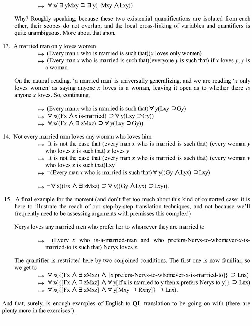
∀x(∃yMxy ⊃∃y(¬Mxy ∧Lxy))

Why? Roughly speaking, because these two existential quantifications are isolated from eachother, their scopes do not overlap, and the local cross-linking of variables and quantifiers isquite unambiguous. More about that anon.

13. A married man only loves women (Every man x who is married is such that)(x loves only women) (Every man x who is married is such that)(everyone y is such that) if x loves y, y isa woman.

On the natural reading, ‘a married man’ is universally generalizing; and we are reading ‘x onlyloves women’ as saying anyone x loves is a woman, leaving it open as to whether there isanyone x loves. So, continuing,

(Every man x who is married is such that)∀y(Lxy ⊃Gy) ∀x((Fx ∧x is-married) ⊃∀y(Lxy ⊃Gy)) ∀x((Fx ∧∃zMxz) ⊃∀y(Lxy ⊃Gy)).

14. Not every married man loves any woman who loves him It is not the case that (every man x who is married is such that) (every woman ywho loves x is such that) x loves y

It is not the case that (every man x who is married is such that) (every woman ywho loves x is such that)Lxy

¬(Every man x who is married is such that)∀y((Gy ∧Lyx) ⊃Lxy)

¬∀x((Fx ∧∃zMxz) ⊃∀y((Gy ∧Lyx) ⊃Lxy)).

15. A final example for the moment (and don’t fret too much about this kind of contorted case: it ishere to illustrate the reach of our step-by-step translation techniques, and not because we’llfrequently need to be assessing arguments with premisses this complex!)

Nerys loves any married men who prefer her to whomever they are married to

(Every x who is-a-married-man and who prefers-Nerys-to-whomever-x-is-married-to is such that) Nerys loves x.

The quantifier is restricted here by two conjoined conditions. The first one is now familiar, sowe get to

∀x({(Fx ∧∃zMxz) ∧ [x prefers-Nerys-to-whomever-x-is-married-to]} ⊃ Lnx) ∀x({[Fx ∧∃zMxz] ∧∀y[if x is married to y then x prefers Nerys to y]} ⊃ Lnx) ∀x({[Fx ∧∃zMxz] ∧∀y[Mxy ⊃ Rxny]} ⊃ Lnx).

And that, surely, is enough examples of English-to-QL translation to be going on with (there areplenty more in the exercises!).

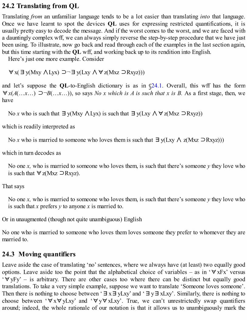
24.2 Translating from QLTranslating from an unfamiliar language tends to be a lot easier than translating into that language.Once we have learnt to spot the devices QL uses for expressing restricted quantifications, it isusually pretty easy to decode the message. And if the worst comes to the worst, and we are faced witha dauntingly complex wff, we can always simply reverse the step-by-step procedure that we have justbeen using. To illustrate, now go back and read through each of the examples in the last section again,but this time starting with the QL wff, and working back up to its rendition into English.

Here’s just one more example. Consider

∀x(∃y(Mxy ∧Lyx) ⊃¬∃y(Lxy ∧∀z(Mxz ⊃Rxyz)))

and let’s suppose the QL-to-English dictionary is as in 24.1. Overall, this wff has the form∀x(A(…x…) ⊃¬B(…x…)), so says No x which is A is such that x is B. As a first stage, then, wehave

No x who is such that ∃y(Mxy ∧Lyx) is such that ∃y(Lxy ∧∀z(Mxz ⊃Rxyz))

which is readily interpreted as

No x who is married to someone who loves them is such that ∃y(Lxy ∧ z(Mxz ⊃Rxyz)))

which in turn decodes as

No one x, who is married to someone who loves them, is such that there’s someone y they love whois such that ∀z(Mxz ⊃Rxyz).

That says

No one x, who is married to someone who loves them, is such that there’s someone y they love whois such that x prefers y to anyone x is married to.

Or in unaugmented (though not quite unambiguous) English

No one who is married to someone who loves them loves someone they prefer to whomever they aremarried to.

24.3 Moving quantifiersLeave aside the case of translating ‘no’ sentences, where we always have (at least) two equally goodoptions. Leave aside too the point that the alphabetical choice of variables – as in ‘∀xFx’ versus‘∀yFy’ – is arbitrary. There are other cases too where there can be distinct but equally goodtranslations. To take a very simple example, suppose we want to translate ‘Someone loves someone’.Then there is nothing to choose between ‘∃x∃yLxy’ and ‘∃y∃xLxy’. Similarly, there is nothing tochoose between ‘∀x∀yLxy’ and ‘∀y∀xLxy’. True, we can’t unrestrictedly swap quantifiersaround; indeed, the whole rationale of our notation is that it allows us to unambiguously mark the

difference between the messages expressed by e.g. ‘∀x∃yLxy’ and ‘∃y∀xLxy’. However,immediately adjacent quantifiers of the same kind can be interchanged.

To labour the point, consider the case where we have neighbouring existential quantifiers. ReadingQL as in 24.1, ‘∃yLny’ attributes to Nerys the property of loving someone. When we quantify in,we get ‘∃x∃yLxy’, which says that someone has the property that ‘∃yLny’ attributes to Nerys (cf. 22.3), i.e. the property of loving someone. So, ‘∃x∃yLxy’ holds just if there is a pair of people inthe domain (not necessarily distinct) such that the first loves the second. Likewise ‘∃xLxn’ attributesto Nerys the property of being loved by someone. Quantifying in, we get ‘∃y∃xLxy’, which saysthat someone has the property that ‘∃xLxn’ attributes to Nerys, i.e. the property of being loved bysomeone. So ‘∃y∃xLxy’ holds just if there is a pair of people in the domain (not necessarilydistinct) such that the first loves the second. That’s the same truth-condition as for ‘∃x∃yLxy’. Andthe point generalizes to any pair of wffs of the form ∃v∃wC(…v…w…), ∃w∃vC(…v…w…).Similarly for pairs of universal quantifiers.

Consider next another sort of case. Suppose we want to translate ‘Nerys is a woman everyoneloves’. The following will in fact do equally well:

(Gn ∧∀xLxn) or∀x(Gn ∧Lxn)

The latter holds just in case everyone x is such as to make it true that (Nerys is a woman and x lovesher), which holds just in case Nerys is a woman loved by everyone, which is what the first says.More generally (borrowing ‘≡’ to express equivalence), we have

(A ∧∀vB(…v…))≡∀v(A ∧B(…v…))

if the variable v doesn’t occur in A. The order of the conjuncts of course doesn’t matter. Similarly, wehave

(A ∧∃vB(…v…))≡∃v(A ∧B(…v…))

if the variable v doesn’t occur in A. Return to example (11) in 1, ‘Someone who is married lovesNerys’. We gave this translation:

∃x(∃yMxy ∧Lxn)

Now we see it would have been equally legitimate to write

∃x∃y(Mxy ∧Lxn)

given the variable ‘y’ does not occur in the second conjunct.And we can do similar manipulations with disjunctions. Suppose we want to translate ‘Either

Owen loves Nerys or nobody does’. We could equally well write

(Lon ∨∀x¬Lxn) or∀x(Lon ∨¬Lxn)

More generally, we have

(A ∨∀vB(…v…))≡∀v(A ∨B(…v…))

where v doesn’t occur in A, and the order of the disjuncts doesn’t matter. Likewise, we have

(A ∨∃vB(…v…))≡∃v(A ∨B(…v…))

The case where we really have to be careful involves conditionals. We have, as you might expect,

(A ⊃∀vB(…v…))≡∀v(A ⊃B(…v…))(A ⊃∃vB(…v…))≡∃v(A ⊃B(…v…))

However, note very carefully the following:

(∀vB(…v…) ⊃A)≡∃v(B(…v…) ⊃ A)(∃vB(…v…) ⊃A)≡∀v(B(…v…) ⊃ A)

Extracting a universal quantification from the antecedent of a conditional (when the variable doesn’toccur in the consequent) turns it into an existential quantification. This shouldn’t be surprising whenyou recall that antecedents of conditionals are like negated disjuncts – remember (A ⊃B) isequivalent to (¬A ∨B) – and recall too that when quantifiers tangle with negation they ‘flip’ into theother quantifier. Consider, for example, the following chain of equivalences:

But having noted the various equivalences in this section for the record, do be very, very cautiousin using them (careless application can lead to trouble)!

24.4 SummaryTranslation into QL can proceed semi-automatically, if (as a half-way house) we transcribevernacular sentences into an augmented English deploying quantifier operators of the kind‘Every/some/no A, v, which is B is such that’, and then use the schemas:

(Every A, v, which is B is such that)Cv ∀v((Av ∧Bv) ⊃Cv)(Some A, v, which is B is such that)Cv ∃v((Av ∧Bv) ∧Cv)(No A, v, which is B is such that)Cv ∀v((Av ∧Bv) ⊃¬Cv)

or ¬∃v((Av ∧Bv) ∧Cv)

The order of neighbouring quantifiers can be swapped if the quantifiers are of the same kind.And quantifiers inside conjunctions and disjunctions can, in certain circumstances, be ‘exported’outside the conjunction/disjunction.

Exercises 24A Suppose ‘m’ denotes Myfanwy, ‘n’ denotes Ninian, ‘o’ denotes Olwen, ‘Fx’ means x is a

philosopher, ‘Gx’ means x speaks Welsh, ‘Lxy’ means x loves y, and ‘Rxyz’ means that x is a childof y and z. Take the domain of discourse to consist of human beings. Translate the following intoQL:

1. Ninian is loved by Myfanwy and Olwen.2. Neither Myfanwy nor Ninian love Olwen.

3. Someone is a child of Myfanwy and Ninian.4. No philosopher loves Olwen.5. Myfanwy and Ninian love everyone.6. Some philosophers speak Welsh.7. No Welsh-speaker who loves Myfanwy is a philosopher.8. Some philosophers love both Myfanwy and Olwen.9. Some philosophers love every Welsh speaker.

10. Everyone who loves Ninian is a philosopher who loves Myfanwy.11. Some philosopher is a child of Olwen and someone or other.12. Whoever is a child of Myfanwy and Ninian loves them both.13. Everyone speaks Welsh only if Olwen speaks Welsh.14. Myfanwy is a child of Olwen and of someone who loves Olwen.15. Some philosophers love no Welsh speakers.16. Every philosopher who speaks Welsh loves Olwen.17. Every Welsh-speaking philosopher loves someone who loves Olwen.18. If Ninian loves every Welsh speaker, then Ninian loves Myfanwy19. No Welsh speaker is loved by every philosopher.20. Every Welsh speaker who loves Ninian loves no one who loves Olwen.21. Whoever loves Myfanwy, loves a philosopher only if the latter loves Myfanwy too.22. Anyone whose parents are a philosopher and someone who loves a philosopher is a

philosopher too.23. Only if Ninian loves every Welsh-speaking philosopher does Myfanwy love him.24. No philosophers love any Welsh-speaker who has no children.

B Take the domain of quantification to be the (the positive whole) numbers, and let ‘n’ denote thenumber one, ‘Fx’ mean x is odd, ‘Gx’ means x is even, ‘Hx’ means x is prime, ‘Lxy’ means x isgreater than y, ‘Rxyz’ means that x is the sum of y and z. Then translate the following into naturalEnglish:

1. ¬∃x(Fx ∧Gx)2. ∀x∀y∃zRzxy 3.∀x∃yLyx 4.∀x∀y((Fx ∧Ryxn) ⊃Gy)3. ∀x∀y((Gx ∧Rxyn) ⊃Fy)4. ∀x∃y((Gx ∧Fy) ∧Rxyy)5. ∀x∀y(∃z(Rzxn ∧Ryzn) ⊃(Gx ⊃Gy))6. ∀x∀y∀z(((Fx ∧Fy) ∧Rzxy) ⊃Gz)7. ∀x(Gx ⊃∃y∃z((Hy ∧Hz)∧Rxyz))8. ∀w∃x∃y(((Hx ∧Hy) ∧(Lxw ∧Lyw)) ∧∃z(Rzxn ∧Ryzn))

C Which of the following pairs are equivalent, and why?

1. ∀x(Fx ⊃Gx); (∀xFx ⊃∀xGx)2. ∃x(Fx ⊃Gx); (∃xFx ⊃∃xGx)3. ∃x(Fx ⊃Gx); (∀xFx ⊃∃xGx)4. ∀x(Fx ⊃Gx); (∃xFx ⊃∀xGx)

The claim that, e.g., that a wff of the form (A ∨∃xFx) is equivalent to one of the form ∃x(A∨Fx) depends on our stipulation that the domain of quantification isn’t empty. Why? Which other

equivalences we stated in 24.3 above also depend on that stipulation?

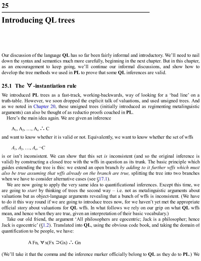
25

Introducing QL trees

Our discussion of the language QL has so far been fairly informal and introductory. We’ll need to naildown the syntax and semantics much more carefully, beginning in the next chapter. But in this chapter,as an encouragement to keep going, we’ll continue our informal discussions, and show how todevelop the tree methods we used in PL to prove that some QL inferences are valid.

25.1 The ∀-instantiation ruleWe introduced PL trees as a fast-track, working-backwards, way of looking for a ‘bad line’ on atruth-table. However, we soon dropped the explicit talk of valuations, and used unsigned trees. Andas we noted in Chapter 20, these unsigned trees (initially introduced as regimenting metalinguisticarguments) can also be thought of as reductio proofs couched in PL.

Here’s the main idea again. We are given an inference

A1, A2, …, An ∴ C

and want to know whether it is valid or not. Equivalently, we want to know whether the set of wffs

A1, A2, …, An, ¬C

is or isn’t inconsistent. We can show that this set is inconsistent (and so the original inference isvalid) by constructing a closed tree with the wffs in question as its trunk. The basic principle whichguides extending the tree is this: we extend an open branch by adding to it further wffs which mustalso be true assuming that wffs already on the branch are true, splitting the tree into two brancheswhen we have to consider alternative cases (see 17.1).

We are now going to apply the very same idea to quantificational inferences. Except this time, weare going to start by thinking of trees the second way – i.e. not as metalinguistic arguments aboutvaluations but as object-language arguments revealing that a bunch of wffs is inconsistent. (We haveto do it this way round if we are going to introduce trees now, for we haven’t yet met the appropriateofficial story about valuations for QL wffs. In what follows we rely on our grip on what QL wffsmean, and hence when they are true, given an interpretation of their basic vocabulary.)

Take our old friend, the argument ‘All philosophers are egocentric; Jack is a philosopher; henceJack is egocentric’ ( 1.2). Translated into QL, using the obvious code book, and taking the domain ofquantification to be people, we have:

A Fn, ∀x(Fx ⊃Gx) ∴ Gn

(We’ll take it that the comma and the inference marker officially belong to QL as they do to PL.) We

show this inference is valid by showing that the premisses and the negation of the conclusion form aninconsistent set. We start by setting down those wffs as the trunk of a tree:

(1) Fn(2) ∀x(Fx ⊃Gx)(3) ¬Gn

Now, how should we extend the tree? Assuming that those wffs are true together, what else has to betrue? Well, if everything in some domain satisfies some condition, then any particular named thing inthat domain satisfies that condition. So if something of the form ∀vC(…v…v…) is true, thenC(…c…c…) will be true, given c names something in the domain. In this case, we are assuming ‘Fn’is true, so ‘n’ certainly should name something in the domain (see 22.4). So the following ought alsobe true:

(4) (Fn ⊃Gn)

And now we can just press on, applying the usual tree-building rule for wffs of the form (A ⊃B); andthe tree closes.

The supposition that the premisses and negated conclusion of A are all true has been revealed to leadto contradiction. Which shows that the argument A is indeed valid.

Another simple example. Consider the inference

B∀x(Fx ⊃Gx), (Fn ∧¬Hn) ∴ ¬∀x(Gx ⊃Hx)

which renders e.g. ‘All logicians are philosophers; Russell is a logician who isn’t wise; so not allphilosophers are wise.’ Again, we assume that the premisses and negation of the conclusion are true,and set down those assumptions as the beginning of a tree.

(1) ∀x(Fx ⊃Gx)(2) (Fn ∧¬Hn)(3) ¬¬∀x(Gx ⊃Hx)

Now we can apply the familiar rules for unpacking the connectives:

(4) Fn(5) ¬Hn(6) ∀x(Gx ⊃Hx)

So far, so straightforward. To proceed further, we evidently need to extract some more ‘n’-relevantinformation. (1) says that any thing x satisfies the condition ‘(Fx ⊃Gx)’. So this will be true inparticular of what ‘n’ denotes. Whence

(7) (Fn ⊃Gn)

Similarly from (6) we have

(8) (Gn ⊃Hn)

Now it is easy to extract an inconsistency. Using the standard rule for the material conditional twice,we have:

And we are done. The assumption that the premisses and the negated conclusion of B are all truetogether leads to contradictions however we try to work through the consequences of that assumption;so the argument is valid.

The new rule for tree-building which we are using here is the ∀-instantiation rule (we’ll call it‘(∀)’ for short). The basic idea is that, given a universal quantification, then any substitution instanceof it must also be true: i.e. any wff which is got by stripping off the quantifier and replacing theremaining occurrences of the associated variable with some name of an object in the domain mustalso be true. But any constant we are already using is supposed to name something in the domain; sothat motivates the following schematic statement of the rule:

(∀) If ∀vC(…v…v…) appears on an open path, we can add C(…c…c…) to the foot ofthe path, where c is any constant which already appears on the path.

Note very carefully that – basically to keep our trees neatly pruned – this rule doesn’t insist that weadd all such instances of the quantified statement to every relevant path whenever we deploy it: therule simply permits us to draw out implications as and where needed. And because we don’t (andindeed can’t) ‘use up’ all the content of the quantified wff in a single application of (∀), we don’tcheck off the quantified wff after applying the instantiation rule.

Here’s a slightly more complex example of our new rule in operation, which illustrates the lastpoint. Consider the argument ‘Every great logician is also a great philosopher; either Moore orRussell is a great logician; so either Moore or Russell is a great philosopher.’ Translating this intoQL, and keeping the domain of quantification to be people, the inference is

C ∀x(Fx ⊃Gx), (Fm ∨Fn) ∴ (Gm ∨Gn)

This is plainly valid. Still, let’s prove that by supposing, in the usual way, that the premisses are trueand the conclusion false, and aiming for contradictions.

We can now use (∀) to extract more ‘m’-related information, instantiate (1) with the name ‘m’ andcontinue the left-hand branch:

Next, consider the right-hand branch. We could have added the wff ‘(Fm ⊃Gm)’ on this branch too,but that won’t do any useful work. What we need to do, in order to develop the right-hand branch, isextract ‘n’-related information from (1) using (∀) again. Now we see the importance of not havingchecked off (1), and marked it as ‘used up’. We hadn’t squeezed all the useful juice out of thatquantified wff; we need to revisit it and extract more implications. This second application (∀)enables us to finish the tree.

The tree closes, and the inference C is shown to be valid.

25.2 Rules for negated quantifiers

We’ve stated the tree-building rule for deducing implications from a wff of the form∀vC(…v…v…).What about a tree-building rule for dealing with a negated universal quantification, i.e. a wff of theform ¬∀vC(…v…v…)?

Well, ¬∀vC(…v…v…) is true just so long as ∃v¬C(…v…v…) is true (see 23.1). Hence apossible rule for treating negated universal quantifications is to transform them into equivalentexistential quantifications, and pass them over to be dealt with by the rule (∃) for dealing withexistential wffs – whatever that rule later turns out to be!

Similarly, note that ¬∃vC(…v…v…) is true just so long as ∀v¬C(…v…v…) is.Hence a possiblerule for treating negated existential quantifications is to transform them into equivalent universalquantifications, and pass them back to be dealt with by the rule for (∀).

We’ll adopt these rules for QL tree-building. Given a wff that starts with a negated quantifier, wecan move the initial negation sign past the quantifier, swapping ‘∀’ with ‘∃’ as it passes. Since thattransformation extracts all the content from the original wff – it takes us from one wff to an exactlyequivalent wff – this time we can check it off after the rule is applied. So schematically:

(¬∀) If ¬∀vC(…v…v…) appears on an open path, then we add the corresponding wff∃v¬C(…v…v…) to each open path that contains it, and check it off.

(¬∃) If ¬∃vC(…v…v…) appears on an open path, then we add the corresponding wff∀v¬C(…v…v…) to each open path that contains it, and check it off.

Let’s review two quick examples of these new rules at work. Consider

D ¬∃x(Fx ∧Gx), Fm ∴ ¬Gm

(Perhaps that translates ‘No logicians are wise; Russell is a logician; so Russell isn’t wise.’) Thecompleted tree looks like this:

At (4) we have applied the new (¬∃) rule to (1); and then we applied (∀) at the next step, and thetree almost immediately closes.

Here’s another intuitively valid argument:

E (Fm ∨Fn), ∀x(Fx ⊃Gx)∴ ∃xGx

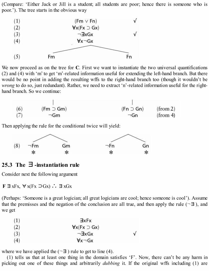
(Compare: ‘Either Jack or Jill is a student; all students are poor; hence there is someone who ispoor.’). The tree starts in the obvious way

We now proceed as on the tree for C. First we want to instantiate the two universal quantifications(2) and (4) with ‘m’ to get ‘m’-related information useful for extending the left-hand branch. But therewould be no point in adding the resulting wffs to the right-hand branch too (though it wouldn’t bewrong to do so, just redundant). Rather, we need to extract ‘n’-related information useful for the right-hand branch. So we continue:

Then applying the rule for the conditional twice will yield:

25.3 The ∃-instantiation ruleConsider next the following argument

F∃xFx, ∀x(Fx ⊃Gx) ∴ ∃xGx

(Perhaps: ‘Someone is a great logician; all great logicians are cool; hence someone is cool’). Assumethat the premisses and the negation of the conclusion are all true, and then apply the rule (¬∃), andwe get

where we have applied the (¬∃) rule to get to line (4).(1) tells us that at least one thing in the domain satisfies ‘F’. Now, there can’t be any harm in

picking out one of these things and arbitrarily dubbing it. If the original wffs including (1) are

consistent, no contradiction can ensue just from this act of selecting and naming. Let’s use a constantthat isn’t currently being used for other purposes – e.g. ‘a’ (for ‘arbitrary’!). So by hypothesis wehave

(5) Fa

What else do we know about the thing now dubbed ‘a’? Given the universal claims (2) and (4), wecan deduce particular claims about it as follows:

The tree closes. To repeat, the mere act of dubbing one of the things which are ‘F’ can’t have createdthe contradiction. So the contradiction must have been in the original assignments of truth to each of(1) to (3). Hence there can be no way of making (1) to (3) all true, and so the inference F is valid.

Another quick example. Take the evidently valid syllogism ‘All logicians are philosophers; allphilosophers are wise; so all logicians are wise.’ Using the obvious translation we get,

G ∀x(Fx ⊃Gx), ∀x(Gx ⊃Hx) ∴ ∀x(Fx ⊃Hx)

We start the tree in the standard way

(1) x(Fx ⊃Gx)(2) x(Gx ⊃Hx)(3) ¬∀x(Fx ⊃Hx)

and apply the (¬∀) rule to get

(4) ∃x¬(Fx ⊃Hx)

(4) tells us that there is at least one thing in the domain such that the condition expressed by ‘¬(Fx⊃Hx)’ holds of it. Pick one, and let’s dub it with a name not otherwise being used in this argument,say ‘a’ again. Then we have

(5) ¬(Fa ⊃Ha)

Applying the (∀) rule to (1) and (2), we get the following further information about this thing dubbed‘a’:

(6) (Fa ⊃Ga)(7) (Ga ⊃Ha)

Then applying the standard propositional rules to (5) to (7) in turn yields

So the tree closes. Again, the contradictions here cannot have been created by the mere act ofselecting and then dubbing something with a name not otherwise in use. Therefore the trouble must bein the original supposition that (1) to (3) are all true; so argument G is valid.

Note that absolutely crucial qualification: contradictions cannot be created by the mere act ofdubbing something with a name not otherwise in use. Of course, if a name has already been recruitedfor some other purpose, then using it again to dub something may very well cause trouble, as we shallnow see.

Consider the following very simple case. The inference ‘Someone is a great philosopher: henceDerrida is a great philosopher’ is obviously bogus. Similarly the inference

H∃xFx ∴ Fn

is equally invalid. Now suppose we start a tree, and then – at line (3) – instantiate the existentialpremiss with the name already in use, to get

(1) ∃xFx(2) ¬Fn

(3) Fn

We have then absurdly ‘proved’ that the fallacious argument H is valid!Here’s another example of the same mistake getting us into trouble. Consider the inference:

I∃xFx, ∃xGx ∴ ∃x(Fx ∧Gx)

Suppose we set out to build a quantifier tree, starting:

(1) ∃xFx(2) ∃xGx(3) ¬∃x(Fx ∧Gx)

We apply the (¬∃) rule to get

(4) ∀x¬(Fx ∧Gx)

Now, if there is at least one thing which satisfies ‘F’, it can do no harm to pick one and dub it ‘a’, sowe could write

(5) Fa

Likewise, if there is at least one thing which satisfies ‘G’, it can do no harm to pick one at dub it withsome name. But suppose we offend by wrongly using the same name again, and add

(6) Ga

to the tree. Given (4), we could continue

The tree then closes, giving the verdict that argument I is valid, which it isn’t! Compare ‘Someone isvery tall; someone is very short; hence someone is very tall and very short.’

It’s evidently step (6) that caused the trouble. To repeat, although (2) tells us that somethingsatisfies ‘G’, and it can do no harm to pick out such a thing and dub it, we mustn’t suppose that it isthe same thing that we have already dubbed ‘a’. At that step (6), we are only entitled to addsomething like

(6) Gb

We could continue

(7) ¬(Fa ∧Ga)

as before, and also add

(8) ¬(Fb ∧Gb)

But this plainly isn’t going to get the tree to close.In summary, then, all this motivates the following ∃-instantiation rule:

(∃)

Given an existential quantification of the form ∃vC(…v…v…) on an open path, thenwe can add C(…c…c…) to each open path that it is on, where c is a ‘new’ constant,i.e. one which hasn’t yet appeared on any of those paths; we then check off theoriginal wff.

∃vC(…v…) tells us that something – and it may be only one thing – is C. So picking such a thing(and dubbing it) exhausts the claim’s commitments: that’s why we need to check it off once the rule(∃) is applied.

Our two proposed rules for un-negated quantifiers might look confusingly similar, so let’s point upthe essential difference loud and clear.

The rule (∀) says that you can instantiate a universal quantifier with any name already in use(on the path).The (∃) rule says that you can instantiate an existential quantifier with any name that isn’talready in use (on the relevant paths).

In Chapter 28, we’ll return to motivate these quantifier tree-building rules much more carefully (butwe’ll need a proper account of the semantics for QL first). However, our quick-and-dirtyexplanations will suffice for the moment.

25.4 More examplesTo help fix ideas, let’s show that the following simple arguments are all valid by translating into QLand using trees (try these examples before reading on):

J Some chaotic attractors are not fractals; all Cantor sets are fractals; hence somechaotic attractors are not Cantor sets.

K If there is a logician who isn’t a philosopher, then Jones isn’t a philosopher. Jones isa philosopher. So every logician is a philosopher.

L Only if Owen is happy does he love someone. If anyone loves Nerys then Owen does.Maldwyn loves Nerys. So Owen is happy.

The first should raise no translational difficulties:

J′∃x(Fx ∧¬Gx), ∀x(Hx ⊃Gx) ∴ ∃x(Fx ∧¬Hx)

and the finished tree looks like this (still adding line numbers for ease of reference):

(1) ∃x(Fx ∧¬Gx) √(2) ∀x(Hx ⊃Gx)(3) ¬∃x(Fx ∧¬Hx) √(4) ∀x¬(Fx ∧¬Hx)(5) (Fa ∧¬Ga) √(6) (Ha ⊃Ga) √(7) ¬(Fa ∧¬Ha) √

How was this tree produced? The first three lines are automatic, and applying the (¬∃) ruleimmediately gives (4). That yields an existentially quantified wff and two universally quantified wffsunchecked.

Now, a useful rule of thumb is where possible apply the (∃) rule before the (∀) rule. Why?Because instantiating an existential quantification always introduces a new name, and you’ll probablyneed to go back to the universal quantifications afterwards to extract any needed information aboutthe named object. But in fact, in this case, we don’t get a choice anyway. The only rule we can applyonce we’ve got to line (4) is the (∃) rule to (1). So we pick one of the things which makes ‘∃x(Fx∧¬Gx)’ true, and dub it ‘a’, yielding (5), and checking off (1). We then extract ‘a’-relevantinformation from (2) and (4) by use of the (∀) rule. With (6) and (7) in place, the rest isstraightforward.

We can translate the next argument thus:

K′ (∃x(Fx ∧¬Gx) ⊃¬Gn), Gn ∴ ∀x(Fx ⊃Gx)

Note carefully the bracketing in the translation of the first premiss. The tree then starts in the standardway, applying the rule (¬∀) to (3):

The left-hand branch now continues

(6) ∀x¬(Fx ∧¬Gx)

(7) ¬(Fa ⊃Ga)

applying first the (¬∃) rule to (5), and then the (∃) rule to (4). Then, after applying the (∀) rule to(6), we quickly finish:

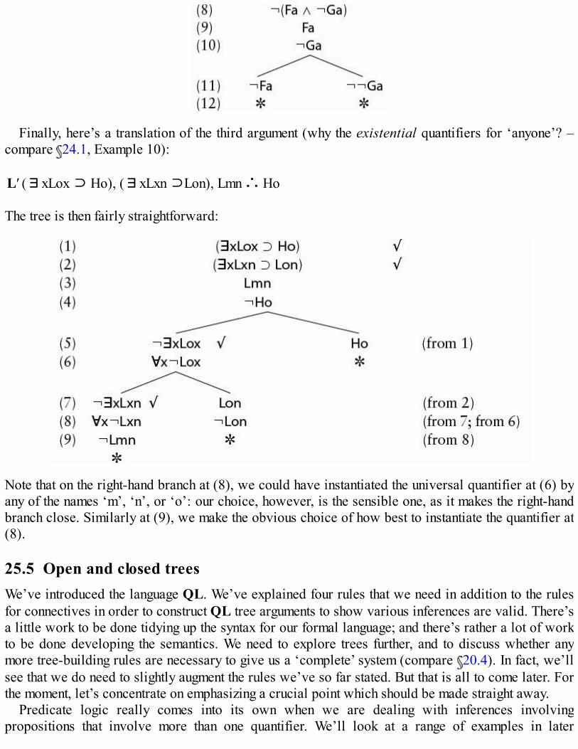
Finally, here’s a translation of the third argument (why the existential quantifiers for ‘anyone’? –compare 24.1, Example 10):

L′ (∃xLox ⊃ Ho), (∃xLxn ⊃Lon), Lmn ∴ Ho

The tree is then fairly straightforward:

Note that on the right-hand branch at (8), we could have instantiated the universal quantifier at (6) byany of the names ‘m’, ‘n’, or ‘o’: our choice, however, is the sensible one, as it makes the right-handbranch close. Similarly at (9), we make the obvious choice of how best to instantiate the quantifier at(8).

25.5 Open and closed treesWe’ve introduced the language QL. We’ve explained four rules that we need in addition to the rulesfor connectives in order to construct QL tree arguments to show various inferences are valid. There’sa little work to be done tidying up the syntax for our formal language; and there’s rather a lot of workto be done developing the semantics. We need to explore trees further, and to discuss whether anymore tree-building rules are necessary to give us a ‘complete’ system (compare 20.4). In fact, we’llsee that we do need to slightly augment the rules we’ve so far stated. But that is all to come later. Forthe moment, let’s concentrate on emphasizing a crucial point which should be made straight away.

Predicate logic really comes into its own when we are dealing with inferences involvingpropositions that involve more than one quantifier. We’ll look at a range of examples in later

chapters; but here’s just one to be going on with (and to set the scene for the point we need to make).Consider the argument ‘Everyone loves someone who is kind; no cruel person is kind; Caligula iscruel. Still, it follows that not everyone is cruel’. That’s evidently valid, if we read the first premissas meaning everyone loves at least one kind person. For take Caligula. Although he is cruel, he lovessomeone who is kind. And that person, being kind, isn’t cruel. So not everyone is cruel.

Let’s warrant this argument with a tree proof. Here’s a translation:

M∀x∃y(Fy ∧Lxy), ∀x(Gx ⊃¬Fx), Gn ∴ ¬∀xGx

The tree starts in the obvious way.

(1) ∀x∃y(Fy ∧Lxy)(2) ∀x(Gx ⊃¬Fx)(3) Gn(4) ¬¬∀xGx √(5) ∀xGx

We now have three universal quantifiers to instantiate, using the rule (∀). But we’ll tackle (1) first,so we can ‘get at’ the embedded existential quantifier. At the moment, we only have one constant inplay, so we have to instantiate (1) with that, to yield

(6) ∃y(Fy ∧Lny)

Now we’ll follow the heuristic rule we noted before: where possible, we apply the (∃) rule beforethe (∀) rule. We have to instantiate (6) with a name new to the argument:

(7) (Fa ∧Lna) √(8) Fa(9) Lna

We can now continue by extracting more ‘a’-relevant information by instantiating the universalquantifications (2) and (5):

And once more we are done.So far, so good. But note we could have taken a wrong turning after line (7). For we might be

struck by the fact that we now have the new name ‘a’ in play, and we could instantiate (1) again withthis new name, thus …

(8′) ∃y(Fy ∧Lay)

We then have a new existential quantification which we can instantiate in turn with a constant new tothe argument:

(9′) (Fb ∧Lab)

Now suppose we (unwisely, but quite legitimately) use the name ‘b’ to instantiate (1) again to infer

(10′) ∃y(Fy ∧Lby)

and instantiate this with respect to a new name:

(11′) (Fc ∧Lbc)

Evidently we could go on, and on, and on without end. The unwise strategy of returning to (1)whenever we can instantiate it with a new name could prevent the tree from ever closing! (Query: butwhat entitles us to suppose that there are all those different things in the domain to be named ‘a’, ‘b’,‘c’, …? Maybe the domain only contains one thing! Reply: the question is based on amisunderstanding. We are introducing a sequence of new names one after another; but maybe thenames refer to the same thing, maybe to different things: that is left open.)

So here we encounter a very deep and important difference between PL and QL trees. In thepropositional case it doesn’t matter (except for the aesthetics) in which order the available rules areapplied. If a tree closes, then any legally constructed tree with the same initial trunk will also close(see 16.4, 19.3). In the quantificational case, by contrast, the order in which rules are appliedmatters. Our first tree for M closed: but we’ve seen that a second tree, equally constructed inaccordance with the rules, could be extended without limit, without closing.

Now, finding one well-constructed closed tree for a QL argument is enough to prove that theargument is valid. If one line of reasoning from the assumption that the premisses and the negation ofthe conclusion are true leads to contradictions all round, that settles it: if the premisses are true, theconclusion must be true too. This result isn’t subverted by the fact that some other line of reasoningtrails off in the wrong direction and fails to reveal a contradiction.

How can QL trees have branches going on for ever when that can’t happen for PL trees? Becauseour rules for unpacking complex PL wffs systematically ‘use up’ wffs, always taking us to shorter andshorter wffs: and – assuming there are only a finite number of premisses to begin with – eventuallywe will simply run out of rules to apply. We must end up with a completed tree, either open or closed.In the quantificational case, however, we can get into cycles like the one that takes us from (6) to (8′)to (10′) to …, where the wffs don’t become any simpler, and so the tree never finishes.

Of course, our second, un-ending, tree for M is constructed according to a pretty crazy strategy.And in fact, there is a decently systematic strategy which will always deliver us a closed tree for anargument if there is one. But intriguingly, there is no mechanical test which will show us (in finitetime) whether applying this strategy will eventually deliver a closed tree; there is no mechanical testfor whether a quantified argument is valid or not. More on this anon (see Chapter 30).

But having seen where all this development of QL is taking us, and in particular having had a

glimpse of how we can develop a tree method for warranting inferences, we really need now toreturn to basics, to tidy up the details. That’s the business for the next few chapters.

25.6 SummaryWe have introduced four new rules for quantifier tree-building, which we’ve labelled (∀),(¬∀), (∃), (¬∃), and given some motivation for them. We’ll state the rules for QL trees morecarefully in Chapter 29.QL trees give us sound proofs of validity: i.e. when a properly constructed tree closes, theargument whose premisses and negated conclusion start the tree is indeed valid. But we notedthat valid arguments can also generate (infinite) open trees.QL trees are not a mechanical method for demonstrating the validity or invalidity of arguments.There can’t be one.

Exercises 25A Show the following simple arguments are valid by translating into QL and using trees.

1. Everyone is rational; hence Socrates is rational.2. No-one loves Angharad; hence Caradoc doesn’t love Angharad.3. No philosopher speaks Welsh; Jones is a philosopher; hence Jones does not speak Welsh.4. Jones doesn’t speak Welsh; hence not everyone speaks Welsh.5. Socrates is rational; hence someone is rational.6. Some philosophers speak Welsh; all Welsh speakers sing well; hence some philosophers sing

well.7. All electrons are leptons; all leptons have half-integral spin; hence all electrons have half-

integral spin.8. All logicians are philosophers; all philosophers are rational people; no rational person is a

flat-earther; hence no logician is a flat-earther.9. If Jones is a bad philosopher, then some Welsh speaker is irrational; but every Welsh speaker

is rational; hence Jones is not a bad philosopher.

B Consider the following rule

(¬∃′) If ¬∃vC(…v…v…) appears on an open path, then we can add ¬C(…c…c…) to that path,where c is any constant which already appears on the path.

Show informally that this rule would do as well as our rule (¬∃). What would be the analogousrule for dealing with negated universal quantifiers without turning them first into existentialquantifiers?

C Suppose we had set up predicate logic with a single quantifier formed using the symbol ‘N’, sothat NvCv holds when nothing is C. Show that the resulting language would be expressivelyequivalent to our now familiar two-quantifier language QL. What would be an appropriate set ofrules for tree-building in a language with this single quantifier?

26

The syntax of QL

Over the last four chapters, we have explored the language QL in an informal way, and we haveintroduced the tree method for warranting quantifier arguments once they are regimented into QLform. In this chapter, we pin down the syntactic details of QL much more carefully, as a preparationfor getting the semantics into clear focus in the next chapter. We start with a couple of preliminarysections, motivating the full-dress syntactic story in 26.3.

26.1 How not to run out of constants, predicates or variablesIn PL, we supplied ourselves with an unlimited number of atomic wffs. That’s because we didn’twant to put a limit on the complexity of arguments that we can express using that language. For exactlythe same reason, we will supply ourselves with an unlimited number of constants and predicates inQL. And we don’t want to run out of variables either, because we want to be able to expresspropositions with arbitrary numbers of quantifiers.

Consider predicates first. Each predicate of QL comes with a fixed number of slots to be filled upwith names (or individual variables). We won’t put any fixed limit on the number of places apredicate can have. Why shouldn’t we be able to argue with five-place or twenty-five-placepredicates?

So we want an unlimited supply of n-place predicates, for each n. Probably the neatest way ofsecuring this is to help ourselves to the numerals. Assume ‘P’ (for ‘predicate’) is in the alphabet ofQL; then we can adopt the rule that any occurrence of this letter with superscript and subscriptnumerals j, k (where j, k ≥ 0) counts as a predicate. The superscript fixes the number of places thepredicate has; and the subscript distinguishes the various predicates which share that number ofplaces. To be sure, it won’t look very pretty having predicates like

but at least we are not going to run out of supplies!We could produce the same effect more in the style of PL by using two sequences of primes (one

sequence to indicate the number of places, and another to distinguish among predicates with the samenumber of places): but that would be typographically even messier.

We’ll adopt the same device of using numerical subscripts to give us unlimited numbers of namesand variables. So we will assume that ‘c’ (for ‘constant’) is in alphabet of QL, and have the rule thatany occurrence of this letter with a subscript numeral k ≥ 0 counts as a constant. Similarly, let’sassume ‘v’ (for ‘varia-ble’) is in the alphabet; there shouldn’t be any confusion with the ‘∨’ sign fordisjunction. The corresponding rule to generate an unlimited number of variables is that anyoccurrence of ‘v’ with a subscript numeral counts as a variable.

By using the subscript trick, we now know we are not going to run out of constants, predicates andvariables.

On the other hand, we most certainly don’t want to be continually writing down ugly wffs like

or worse. Nor do we want retrospectively to rule out all our examples over recent chapters fromcounting as official wffs of QL. So, although it complicates things, let’s also add to our vocabularyall the unadorned letters for names, predicates, and variables that we’ve met before, plus a few extra.

One last comment. A three-place predicate like takes three names to form an atomic wff of QL.What about a zero-place predicate like (for note, we did allow the superscript indicating thenumber of places to take the value zero)? By parity of reasoning, a zero-place predicate is anexpression that takes zero names to make an atomic wff – in other words, it already is an atomic wff!So a zero-place predicate functions exactly like a propositional atom of PL. This has the kind ofneatness that mathematically inclined logicians just love. Instead of saying that our language QL hasboth predicates of all degrees from one upwards plus propositional atoms as well, we say morecrisply that the language has predicates of all degrees from zero upwards. (It could be convenient,however, to have a few simple letters for propositional atoms in addition to the zero-superscriptedinstances of ‘P’. Since ‘P’ and ‘R’ are already recruited for other uses, let’s add ‘A’, ‘B’, ‘C’ for thispurpose. By this stage in the game, no-one is going to confuse these object-language sans-serif letterswith the italic letters ‘A’, ‘B’, ‘C’ we use as metalinguistic schematic variables when generalizingabout wffs).

26.2 How to introduce quantifiersIn Chapter 22, we showed how we can build up quantified wffs by the operation of quantifying in.We take a wff with a constant in it, and then – in one go, so to speak – we replace the constant with avariable and also prefix a quantifier formed using that same variable (thereby ‘binding’ the variableto the quantifier). To take the simplest kind of example, we can start from the atomic wff ‘Fm’, andquantify in to form the wff ‘∃x Fx’.

Here’s an alternative way of proceeding. We could say that atomic wffs are formed by combining apredicate with the right number of constants and/or variables. So, by this more generous rule foratomic wffs, ‘Fx’ is itself a wff. Then the rule for adding quantifiers is: given a wff C(…v…v…)involving one or more occurrences of the variable v, but not already containing the quantifier ∀vor∃v, then we form another wff by prefixing one of those quantifiers. So since ‘Fx’ is a wff by ourfirst new rule, ‘∃xFx’ is a wff by the new second rule. (This second rule says we can only prefixquantifiers that link to variables that aren’t already tied to quantifiers. That prevents us going on toform expressions like ‘∃x∃xFx’ or ‘∃y∃xFx’.)

In Chapter 22, we quickly demonstrated that ‘∀y∀x∃zRzyx’ is a wff by setting out a possibleway of constructing it by three operations of quantifying in, with the following sequence of steps:

Rmno∃zRzno∀x∃zRznx∀y∀x∃zRzyx

Note, by the way, that we could equally well have followed the steps

Rnom∃zRzom∀x∃zRzox∀y∀x∃zRzyx

So on our previous story, wffs don’t have a unique ‘constructional history’ (cf. 8.2). But given ournew rules, to construct the same wff, we instead start from ‘Rzyx’ and simply add the quantifiers likethis:

Rzyx∃zRzyx∀x∃zRzyx∀y∀x∃zRzyx

and this constructional history is unique under our new rules. That’s one differ-ece between the oldand new rules. But the key difference between our two ways of proceeding is that on the new one,expressions with variables ‘dangling free’, like ‘Rzyx’ or ‘∀x∃zRzyx’ count as wffs, which theydidn’t before. Every old-style wff is a new-style wff, but not vice versa.

Quantifiers in QL need variables, and the point of variables is to be tied to quantifiers; so ourapproach in Chapter 22, where they get introduced in tandem is in some ways the more natural one.But the more liberal two-step approach, which also allows wffs with ‘free’ variables, has somepresentational advantages when we turn to technicalities. And perhaps more to the point, it is still themore common approach (to the extent that it would be odd to study quantificational logic and neverhear of wffs with free variables). We’ll follow the common convention and adopt the more liberalrules for forming wffs from now on.

26.3 The official syntaxWe’ll now put together all the ideas about syntax from Chapter 22, and from 26.1, 26.2 above, intoone composite story. This is done for convenience and for the sake of completeness; there are no newideas here. We state the rules using metalinguistic variables like ‘A’ and ‘v’ in the now familiar way.

The official syntax for QL

The alphabet for QL is as follows:

for forming constants: a,b,c,m,n,ofor forming predicates: A,B,C,F,G,H,L,M,P,R,Sfor forming variables: v,w,x,y,zfor superscripts and subscripts: the arabic numeralsfor constructing complex wffs: ∧, ∨, ¬, ⊃, ∀, ∃, (, )for expressing arguments: ∴, , plus also the comma.

The basic elements of QL are then:

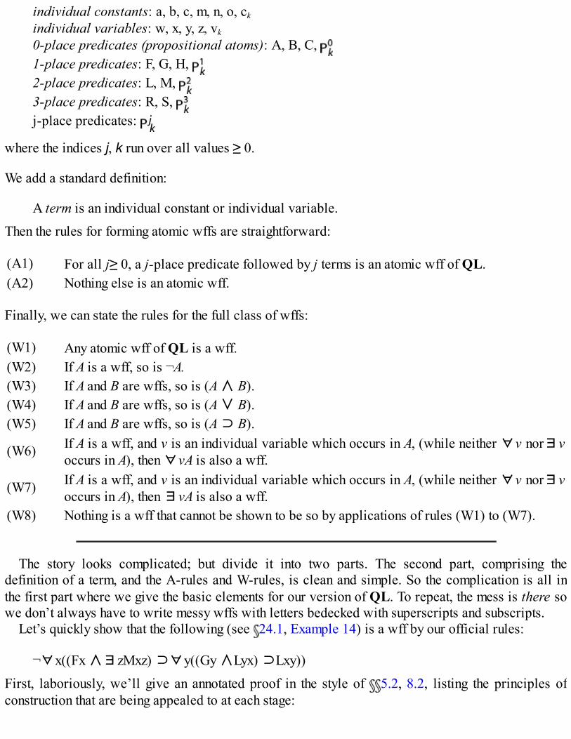
individual constants: a, b, c, m, n, o, ck

individual variables: w, x, y, z, vk

0-place predicates (propositional atoms): A, B, C, 1-place predicates: F, G, H, 2-place predicates: L, M, 3-place predicates: R, S, j-place predicates:

where the indices j, k run over all values ≥ 0.

We add a standard definition:

A term is an individual constant or individual variable.

Then the rules for forming atomic wffs are straightforward:

(A1) For all j≥ 0, a j-place predicate followed by j terms is an atomic wff of QL.(A2) Nothing else is an atomic wff.

Finally, we can state the rules for the full class of wffs:

(W1) Any atomic wff of QL is a wff.(W2) If A is a wff, so is ¬A.(W3) If A and B are wffs, so is (A ∧ B).(W4) If A and B are wffs, so is (A ∨ B).(W5) If A and B are wffs, so is (A ⊃ B).

(W6) If A is a wff, and v is an individual variable which occurs in A, (while neither ∀v nor∃voccurs in A), then ∀vA is also a wff.

(W7) If A is a wff, and v is an individual variable which occurs in A, (while neither ∀v nor∃voccurs in A), then ∃vA is also a wff.

(W8) Nothing is a wff that cannot be shown to be so by applications of rules (W1) to (W7).

The story looks complicated; but divide it into two parts. The second part, comprising thedefinition of a term, and the A-rules and W-rules, is clean and simple. So the complication is all inthe first part where we give the basic elements for our version of QL. To repeat, the mess is there sowe don’t always have to write messy wffs with letters bedecked with superscripts and subscripts.

Let’s quickly show that the following (see 24.1, Example 14) is a wff by our official rules:

¬∀x((Fx ∧∃zMxz) ⊃∀y((Gy ∧Lyx) ⊃Lxy))

First, laboriously, we’ll give an annotated proof in the style of 5.2, 8.2, listing the principles ofconstruction that are being appealed to at each stage:

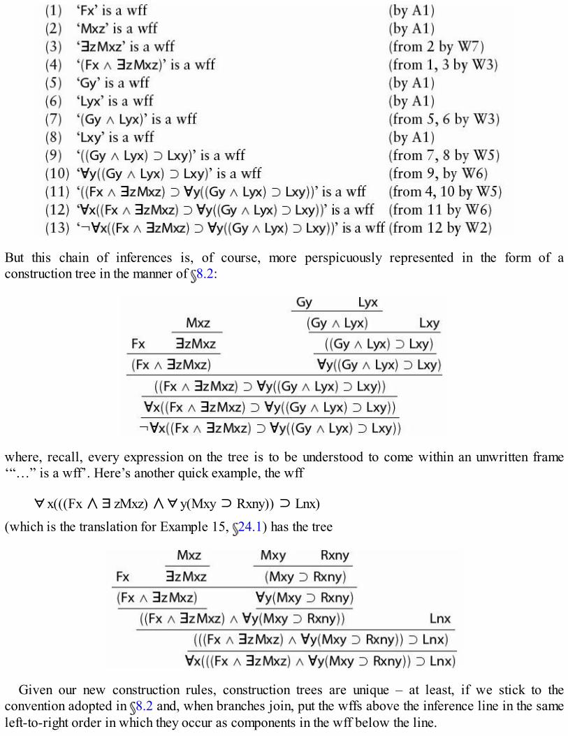
But this chain of inferences is, of course, more perspicuously represented in the form of aconstruction tree in the manner of 8.2:

where, recall, every expression on the tree is to be understood to come within an unwritten frame‘“…” is a wff’. Here’s another quick example, the wff

∀x(((Fx ∧∃zMxz) ∧∀y(Mxy ⊃ Rxny)) ⊃ Lnx)

(which is the translation for Example 15, 24.1) has the tree

Given our new construction rules, construction trees are unique – at least, if we stick to theconvention adopted in 8.2 and, when branches join, put the wffs above the inference line in the sameleft-to-right order in which they occur as components in the wff below the line.

One more construction tree, this time for

∀x(∃yMxy ⊃∃y(¬Mxy ∧Lxy))

(the second version of the translation for Example 12, 24.1). The variable ‘y’ in the end getsquantified twice; we want to show that this is legitimate.

Note that the two ‘∃y’quantifiers get introduced on separate branches of the tree. At eachintroduction, left and right, the quantifier is applied to a wff where the variable ‘y’ occurs and hasn’tyet been quantified. So the construction follows our rules. Compare

∀x(Fx ⊃∃x(Gx ∧Lxn))

which isn’t a wff by our rules. If we try to produce a tree, we could get as far as showing that ‘Fx’and ‘∃x(Gx ∧Lxn)’ are wffs, and so

(Fx ⊃∃x(Gx ∧Lxn))

is a wff. But we can’t use (W6) to add the quantifier ‘∀x’, because that last wff already contains oneof the quantifiers ‘∀x’ or ‘∃x’.

26.4 Some useful definitionsWe’ll define (or redefine) some useful syntactic notions. First, as in PL,

A wff A is a subformula of a wff B if A appears anywhere on the construction tree for B.

And, similarly to PL,

The main logical operator (quantifier or connective) of A is the operator introduced at the finalstep in the construction tree.

Next, we want to capture the idea of an expression being within the scope of an operator (quantifieror connective). As in 8.2, a neat way of doing this is to define some wff as being the scope of anoperator, and then any part of this wff will count as being in the scope of the operator:

The scope of a quantifier in a QL wff is the subformula that starts with that quantifier. In otherwords, it is the wff that occurs at the step on the construction tree where the quantifier isintroduced. Take for example the wff ‘∀x(∃yMxy ⊃∃y(¬Mxy ∧Lxy))’:

the scope of the first ‘∃y’ is ‘∃yMxy’;the scope of the second ‘∃y’ is ‘∃y(¬Mxy ∧Lxy)’;the scope of ‘∀x’ is the whole wff.

The scope of a connective is likewise the wff on the construction tree where the connective isintroduced.

Now let’s tidy up the intuitive notion of a ‘free’ variable. The idea is that a variable dangles freewhen it isn’t tied down by a matching quantifier. So let’s say

An occurrence of a variable v in a wff A is bound if and only if it is in the scope of somematching quantifier ∀v or ∃v that occurs in A.An occurrence of a variable v in a wff A is free if and only if it is not bound.

Thus consider the wffs

(Mxy ⊃ Rxny)∀y(Mxy ⊃ Rxny)((Fx ∧∃zMxz) ∧∀y(Mxy ⊃ Rxny))

In the first, both variables are free. In the second, ‘y’ is bound and ‘x’ is free. In the third, ‘y’ and ‘z’are both bound, but ‘x’ still remains free. Again, in

(Mxy ⊃∃y(¬Mxy ∧Lxy))

which counts as a wff by our rules, the first occurrence of ‘y’ is free but the others are bound (so wecan’t quantify the whole wff using ‘∀y’ again).

With that terminology now to hand, the rules (W6) and (W7) come to this: If A is a wff, and v is anindividual variable which only occurs free in A, then ∀vA and∃vA are also wffs.

We need a term for those wffs without any occurrences of variables remaining free:

A sentence of QL (alternatively, a closed wff) is a wff with no free occurrences of variables.If a wff isn’t closed it is open.

If ‘F’ means … is wise, then (remembering that variables operate like pronouns) we might read anopen wff like ‘Fx’ as meaning something like he is wise. But taken as a stand-alone claim, withoutanything to tell us who ‘he’ is referring to, this doesn’t express a determinate proposition: it isn’t yeteither true or false. By contrast, closed wffs can be true or false.

Finally, we define again the notion of a substitution instance of a quantified wff ( 22.4):

Suppose a wff C(…c…c…) results from ∀vC(…v…v…) or ∃vC(…v…v…) by stripping offthe initial quantifier, and then substituting some individual constant c for all the occurrences ofthe associated variable v. Then C(…c…c…) is said to be an instance of the quantified sentence.

26.5 SummaryWe have now taken a semi-permissive line on what is to count as an official wff of QL. We are

allowing wffs with free variables, though we are still ruling out expressions with redundant orduplicated quantifiers.We have given ourselves an unlimited supply of predicates, names and variables, usingnumerical subscripts and superscripts.The key building rule for constructing quantified sentences is: if A is a wff, and v is an individualvariable which only occurs free in A,∀vA and ∃vA are also wffs.Demonstrations that an expression is indeed a wff according to our rules can be set out asconstruction trees; looking at how the tree is built up will reveal the scope of the various logicaloperators, and which occurrences of variables are free at which stage of the construction.

Exercises 26Which of the following are wffs of QL? Which are sentences, i.e. closed wffs? In the open wffs,which occurrences of which variables are free? What is the main logical operator of each wff?

1. ∃z∀y(Myz ∨¬∀y(Mxy ∧Lxy))2. ∃z(∀yMyz ∨¬(Mxy ∧Lxy))3. ∃z(∀yMyz ∨¬∀y(Mxy ∧Lxy))4. ¬∃z(∀yMyz ∨¬∀x∀y(Mxy ∧Lxy))5. ∃z∀x(∀yMyz ∨¬∀y(Mxy ∧Lxy))6. ∀x(Gx ⊃∃y∃z(Hy ∧Hz) ∧Rxyz))7. (Gx ⊃∃x∃z((Hy ∧Hz) ∧Rxyz))8. ∀x∃y(Gx ⊃∃y¬∃z((Hy ∧Hz) ∧Rxyz))9. ∀x(Gx ⊃∃y∀x((Hy ∧Hz) ∧Rxyz))

10. (∀x(Gx ⊃∃z((Hy ∧Hz) ∧Rxyz)) ∨∃zHz)11. ∀x∀y∀z((Fx ∧Fy) ∧Rzxy) ⊃Gz)12. ¬∀x∀y(((Fx ∧Fy) ∧∀zRzxy) ⊃Gz)

27

Q-valuations

Having now tidied up the syntax, in this chapter we give the official story about the semantics of QL.In particular, we define the key notion of a q-valuation of QL wffs (the analogue of a truth-valuationfor PL).

27.1 Q-valuations vs. interpretationsWhen describing the semantics for PL in Chapter 9, we quickly moved on from discussinginterpretations of wffs to discussing valuations. A valuation, recall, starts with an assignment oftruth-values to some of the building blocks of PL (i.e. some atomic wffs). This initial assignment thengenerates a valuation of all the molecular wffs that can be built up from these atomic wffs using thelogical resources of the language (i.e. the connectives). We also defined the notion of tautologicalvalidity – where an inference is tautologically valid if every valuation which makes the premissestrue makes the conclusion true. Tautological validity implies plain validity; but there are validarguments (e.g. a PL translation of ‘Jo is a sister, hence Jo is female’) which are not tautologicallyvalid.

We now proceed similarly, by introducing the notion of a q-valuation. An interpretation of (some)QL wffs tells us what the relevant wffs mean; a q-valuation fixes which of these wffs are true. A q-valuation must start by fixing the domain of discourse; then it needs to assign truth-relevant values tosome of the building blocks of QL (i.e. some constants and predicates). This initial assignment thengenerates a valuation of all the wffs that can be built up from these ingredients using the logicalresources of the language. In particular it tells us which closed wffs (sentences, wffs without freevariables) are true. We can then define the key notion of q-validity, where an inference is q-valid ifevery q-valuation which makes the premisses all true makes the conclusion true. Q-validity impliesplain validity; but there are valid arguments (e.g. a QL translation of ‘Jo is a sister, hence Jo isfemale’) which are not q-valid.

Valuations are crucial for propositional logic, thought of as the study of arguments that are validbecause of the way that the truth-functional connectives distribute among premisses and conclusion.Q-valuations are crucial for quantificational logic, thought of as the study of arguments that are validbecause of the way connectives and quantifiers distribute among premisses and conclusion.Irritatingly and confusingly, you will find q-valuations are elsewhere usually called ‘interpretations’.But an interpretation (in the intuitive sense of the term, which accords with our use in this book) givesthe meaning or sense of some expressions: by contrast, a q-valuation just specifies the features ofthese expressions which fix the truth-values of wffs.

27.2 Q-valuations defined

Given a bunch of QL wffs, let’s say that their vocabulary is the set V of constants and predicates thatappear in those wffs. So a q-valuation for a set of wffs with vocabulary V needs to (1) fix a domain Dfor the quantifiers to run over, and then assign truth-relevant properties to (2) the constants and (3) thepredicates in V.

(1) We’ll allow the domain D to be any collection of objects, big or small. The domain might be a‘natural’ set like all people, or all numbers. But any old gerry-mandered collection, such as the set{The Eiffel Tower, the number four, Bill Clinton, Mount Everest} – or even the tiny set {JenniferLopez} containing just one item, namely Jennifer – can also serve as a domain of discourse.

Could we allow the domain to contain absolutely everything? It isn’t clear that this idea makessense. For take a domain as big as you like. Then isn’t there always a more inclusive collection ofthings containing all the objects in the original domain plus something else, namely the set of thoseobjects? But we won’t tangle here with that kind of issue. We’ll just allow domains to be anydeterminate collection of objects, however big that might possibly be.

To go to the other extreme, could we allow the domain to be empty, to have nothing in it? Thereare pros and cons to the proposal that we should allow empty domains. Tradition is on the side ofrequiring that any domain contains at least one object; and, as we’ll see, some technicalities do gomore smoothly if we follow tradition. So we’ll take the standard line and require domains to benon-empty. More on this in 29.3.

(2) Consider an ordinary-language sentence like ‘Bill is wise’. What is required for this to be true? Acertain man has to be wise. And the role of the name ‘Bill’ is to pick out the individual who has to bewise if the sentence is to be true. In other words, what matters about the name here, as far as truth isconcerned, is to whom it refers.

To be sure, there can be differences in associations, tone, or sense between names that have thesame reference, like ‘Bill’ and ‘Mr Clinton’. But as far as the truth of what we say goes, it normallydoesn’t matter which name we use. For example, ‘Bill kissed Monica’ and ‘Mr Clinton kissedMonica’ attribute the same action to the same man, and hence are true or false together.

Constants are the QL analogues of ordinary-language names. So similarly, what matters about aconstant, as far as truth is concerned, is which object it refers to. Or as we’ll say: the q-value of aconstant is its reference. Of course, this object should be in the domain of discourse; for the referenceof a constant c should be one of the things that is in question when we talk of ‘everything’!

(3) The third component of a q-valuation deals with predicates. Again, we take our lead fromelementary reflections about their ordinary-language correlates.

‘Bill is wise’ is true just if the man picked out by the name ‘Bill’ is one of the wise. That way ofputting it immediately suggests a simple way of looking at what matters about ‘… is wise’ as far astruth is concerned. The predicate is correlated with a set of things – the things that satisfy thecondition of being wise. If Bill is in that set, the sentence in question is true; if not, not.

The set of objects that satisfy a predicate is standardly called the extension of the predicate. Soanother way of putting things is this: a sentence like ‘Bill is wise’ is true just if the object referred toby the name is in the extension of the predicate. (Maybe no one is wise: in that case the extension ofthe predicate is empty.)

Moving from ordinary language to QL, we again can say that (as far as truth is concerned) whatmatters about a one-place predicate is its extension, the set of objects of which the predicate is true.

These objects should be in the domain D; the things of which a predicate is true should again beamong the things which count as ‘everything’. So the q-value of a one-place predicate F is a (possiblyempty) set of objects from the domain. And an atomic wff of the form Fc will be true if and only if theq-value of c (i.e. the object which c refers to) is in the q-value of F (i.e. is in the extension of F).

What about evaluating two-place predicates? Well, ‘Romeo loves Juliet’ is true just so long as thepair of people Romeo, Juliet is in the set of pairs such that the first in the pair loves the second.So what matters about a relational term like ‘loves’ is the set of pairs of things it picks out: this set ofpairs is the extension of the relation. Likewise for two-place relations in QL. The q-value of a two-place relation R is its extension, a set of pairs of things from the domain. And a wff of the form Rmnis true if and only if the q-values of the constants m and n taken in that order form a pair that belongsto the extension of R. (When we talk about pairs here, we of course mean ordered pairs, so that wecan indeed sensibly talk of a first and second member.)

Similarly, the q-value of a three-place relation S is a set of ordered triples (namely, the triples thatsatisfy S). A wff of the form Smno is true if the q-values of the names taken in order form an orderedtriple which is in the extension of the predicate. And so it goes.

It is useful to introduce some standard jargon here. We’ve spoken of individual objects, orderedpairs or couples, and ordered triples. What comes next, of course, are ordered quadruples,quintuples, and so on. So let’s refer to all such items as tuples: tuples with n members are, of course,n-tuples. We can then snappily say: for n > 0, the q-value of an n-place predicate is a set of n-tuples.(That works, at any rate, if we stipulate that ‘1-tuples of objects’ are just the objects.)

But remember, we are also allowing zero-place predicates in QL ( 25.1). Such expressions arealready atomic wffs in their own right, just like the propositional variables in PL. If there are anysuch expressions in the vocabulary V, then we will give them their own distinctive kind of values on aq-valuation, namely truth-values.

So putting all that together, we have the following definition:

A q-valuation defined over vocabulary V:

(1) specifies a (non-empty) collection of objects to be the domain D;(2) it assigns to any constant in V some object in D as its q-value;(3) it assigns a truth-value to any 0-place predicate in V; and it assigns to any n-place predicate in

V, where n > 0, a (possibly empty) set of n-tuples of objects from D.

27.3 The semantics of quantifiers: a rough guideA q-valuation defined over the vocabulary V fixes the truth-values for atomic sentences built fromconstants and predicates in V in the obvious way. An atomic sentence formed from an n-placepredicate followed by n constants is true just in case the n-tuple formed by taking the q-values of then constants in order is in the extension of the n-place predicate (except for the special case where n =0, when the q-valuation directly assigns the 0-place predicate its own truth-value).

Further, we’ll let QL’s truth-functional connectives look after themselves for the moment in theobvious way (so it will still be the case that a conjunction is true if both the conjuncts are true, and soon and so forth).

So the key question is how to deal semantically with quantified wffs. For example, when is the wff

‘∀xFx’ true?

We remarked before on a wrong answer. We can’t say that ‘∀xFx’ is true just when all itssubstitution instances in the given vocabulary V are true, i.e. when ‘Fm’, ‘Fn’, ‘Fo’, … are alltrue. There may not be names in V for every object in the domain; so even if all the instances wecan construct are true, ‘∀xFx’ could still be false, because of an uncooperative unnamed object(see 22.4).To introduce a correct answer, note that ‘Every man is such that he is mortal’ is true just so longit doesn’t matter which man in the domain we choose, he is mortal – i.e. if ‘He is mortal’ is true,whoever we use the pronoun ‘he’ to point to in the domain of men. We can say somethingsimilar about ‘∀xFx’ (for recall that we introduced variables in QL to do the work of pronouns,and remember too that we are now allowing expressions with free variables to count as wffs).So, ‘∀xFx’ is true if ‘Fx’ is true when ‘x’ is treated as a pronoun pointing to an object in thedomain, no matter which object in the domain the pronoun is taken to be picking out.

The rejected answer wrongly tries to explain when ‘∀xFx’ is true by generalizing about names. Ournew, correct, suggestion explains when it is true by generalizing about objects in the domain.

Following that lead, consider three wffs of the forms

(a) ∀vC(…v…v…)(b) ∃vC(…v…v…)(c) C(…v…v…)

Then the key idea is that (a) is true if the corresponding wff (c) comes out true when v is treated as apronoun, no matter what object in the domain the pronoun v is taken to be ‘pointing to’. Likewise (b)is true when there is some object in the domain such that (c) comes out true when v is treated as apronoun picking out that object.

This straightforward and entirely intuitive idea is the key that unlocks the semantics of quantifiers.Everything that follows in the rest of this chapter just develops this one idea a bit more formally; itshould be easy enough to grasp the official version as long as you don’t lose sight of this underlyingmotivation.

So, to develop the key idea, we now allow q-valuations to be extended to valuations which assigntemporary references to one or more variables. Take the simplest case where just one variable v isinvolved:

We extend a given valuation q by assigning an object o from the domain for v to ‘pick out’ whenthe variable occurs free. Call this extension q+. We can then treat wffs with free occurrences of vas if the variable is a temporary name for the object o assigned to the variable by q+. So,vC(…v…v…) is true on q just if C(…v…v…) is true on every possible extension q+ giving areference to v – i.e. no matter what object o in the domain is assigned to v, C(…v…v…) stillcomes out true when v is treated as a pronoun referring to o. Similarly, ∃vC(…v…v…) is trueon q if C(…v…v…) is true on some extension q+.

Let’s take a simple example. Suppose we are interpreting items in the vocabulary V = {‘m’, ‘F’, ‘L’}

to mean, respectively, Socrates, … is a philosopher, and … loves …, and we understand thequantifiers as running over all people (past and present). Then the corresponding q-valuation q willsay:

(1) the domain of discourse is the set of all people;

(2) ‘m’ refers to Socrates (i.e. has Socrates as its q-value);

(3) the extension of ‘F’ is the set of philosophers; and the extension of ‘L’ is the set ofpairs of people such that the first loves the second.

Helping ourselves to the obvious rules for the connectives, we can now work out the value of the wff

(a) ∃x(Fx ∧Lmx)

(translation: Socrates loves some philosopher). This is true so long as there is some extension q+ ofq, which assigns an object in the domain to ‘x’, which makes

(a*) (Fx ∧Lmx)

come out true. Which there is. Take the extension q+ which assigns Plato to ‘x’. Then, with thevariable/pronoun treated as referring expression picking out Plato, ‘Fx’ is true since Plato is in the setof philosophers; and ‘Lmx’ is true since the pair Socrates, Plato is famously in the set of pairssuch that the first member of the pair loves the second. Hence the conjunction ‘(Fx ∧Lmx)’ is true onq+.

Now compare

(b) ∀x(Fx ⊃Lmx)

(translation: Socrates loves every philosopher). This comes out false. For (b) is true only if

(b*) (Fx ⊃Lmx)

is true on every possible extension q+ of q. But consider the extension q+ which assigns BertrandRussell to ‘x’. Russell is in the set of philosophers, so ‘Fx’ is true on q+. ‘Lmx’ is false, because thepair Socrates, Russell is presumably not in the set of pairs such that the first member of the pairloves the second. So this q+ makes the antecedent of (b*) true and its consequent false, so makes (b*)false. Hence (b*) isn’t true on all possible extensions of q; so (b) is indeed false on the original q-valuation.

So far, so good. Things get only a little more complicated when have to deal with wffs involvingmore than one quantifier. We then have to consider extended valuations which assign references tomore than one variable. Take for example

(c) ∃y∃x(Fx ∧Lyx)

(translation: There’s someone who loves a philosopher). (c) is true on our valuation q so long as

(c*) ∃x(Fx ∧Lyx)

is true on some possible extension q+ which assigns a reference to the variable ‘y’. One suchextension q+ assigns Socrates to ‘y’. So let’s ask, is (c*) true on q+? Well, (c*) will be true on thatvaluation if there is some further extension q++ which as well as assigning Socrates to ‘y’ alsoassigns someone to ‘x’, where

(c**) (Fy ∧Lxy)

is true on q++. And there is such an extension – assign Plato to ‘x’ again!What about

(d) ∀y∃x(Fx ∧Lyx)

(translation: Everyone loves some philosopher)? This is true on q if for every extension q+ whichassigns a reference to ‘y’ there is a further extension q++ which assigns a reference to ‘x’ which makes(c**) true.

And so it goes. The main ingredients for our official story about the semantics of QL are now inplace. And it should already seem plausible that, however complex a closed QL wff W is, a q-valuation for its vocabulary suffices to fix W’s truth-value (just as a valuation of the atoms in acomplex PL wff fixes the truth-value of that wff). And generalizing: a q-valuation defined over thevocabulary V of some set of closed wffs Σ will similarly fix the truth-values of every wff in Σ.

The rest of this chapter just wraps up these ideas into an official story presented rather moreformally. But if you find that kind of more abstract presentation hard going, just skim and skip, or evenomit. Our informal presentation so far is all you really need to know.

27.4 The official semanticsTo summarize so far. The standard truth-valuational story about PL gives rules for working out thetruth-values of more complex wffs in terms of the values of their simpler constituent subformulae (9.4). We now want to give similar rules for working out the values of complex QL wffs in terms ofthe q-values of their constituents. En route, we will want to say how the value of the wff ‘∀xFx’relates to valuations of its subformula ‘Fx’, and similarly how the value of ‘∀y∃x(Fx ∧Lyx)’relates to valuations of its subformulae, ultimately ‘Fx’ and ‘Lyx’. But of course, those subformulaedon’t have a truth-value on a q-valuation just of constants and predicates. In order to do systematicsemantics, going via these subformulae with free variables, we are going to have to follow the idea ofthe last section and consider extended valuations which treat variables as if they have temporaryreferences. And the truth of ‘Fx’ on one extended valuation won’t ensure the truth of ‘∀xFx’. As wesaw, we have to generalize over extended valuations to give the right truth-conditions for quantifiedwffs.

So first, let’s augment the definition in the previous box ( 27.2) by defining extended valuations.That’s easy: Henceforth, we’ll use ‘(extended) valuation’ to cover both original q-valuations

An extended q-valuation defined over vocabulary V is a q-valuation defined over V, augmentedby an assignment of objects as q-values to one or more variables.

Henceforth, we’ll use ‘(extended) valuation’ to cover both original q-valuations and extended ones.We are also going to need the following definition: If q doesn’t assign any object to v already, then av-variant q′ will of course

An extended q-valuation q′ is a v-variant of the (extended) valuation q if q′ assigns some objecto as q-value to the variable v and otherwise agrees exactly with q.

If q doesn’t assign any object to v already, then a v-variant q′ will of course extend q by giving avalue to v. If q does already assign an object to v, then a v-variant q′ may (but needn’t) change thatassignment. To revisit an example from the last section, suppose q is the q-valuation defined over{‘m’, ‘F’, ‘L’} that we met before; q1 is just the same, except that it also assigns Socrates to ‘x’; andq2 is the same as q except it assigns Plato to ‘x’. Then q1 is an ‘x’-variant of q (and of q2), and q2 is an‘x’-variant of q1 (and of q).

With that notion to hand we can neatly give the rules that determine the truth value of any wff builtfrom vocabulary V, on some valuation q which covers V. First, we need the rule (Q0) to deal with theatomic wffs on valuations extended or otherwise (recall, ‘term’ means ‘constant or variable’, see 26.3):

(Q0)

An atomic wff, i.e. an n-place predicate followed by n terms, is true on the (extended)valuation q if either n = 0, and the q-value of the 0-place predicate is true, or else n > 0,and the n-tuple formed by taking the q-values of the terms in order is in the extensionwhich is the q-value of the n-place predicate. Otherwise it is false.

Second, here are the clauses to cover the various ways in which the truth-values of more complexwffs depend on the values of simpler ones. For brevity, we use ‘⇒q T’ to mean ‘is true on the(extended) q-valuation q’ (dropping quotation marks before ‘⇒’; see 16.3). Each clause is of courseintended apply to any valuation, and so can be read as if prefixed by ‘For all (extended) valuations q,…’:

(Q1) For any wff A, ¬A ⇒q T if A ⇒q F; otherwise ¬A ⇒q F.(Q2) For any wffs A, B: (A ∧B) ⇒q T if both A ⇒q T and B ⇒q T; otherwise (A ∧B) ⇒q F.(Q3) For any wffs A, B: (A ∨B) ⇒q F if both A ⇒q F and B ⇒q F; otherwise (A ∨B) ⇒q T.(Q4) For any wffs A, B: (A ⊃B) ⇒q F if both A ⇒q T and B ⇒q F; otherwise (A ⊃B) ⇒q T.

(Q5) For any wffs A, B: (A≡B) ⇒q T if either both A ⇒q T and B ⇒q T, or both A ⇒q F and B⇒q F; otherwise (A≡B) ⇒q F.For any wff C(…v…v…) with variable v free, ∀vC(…v…v…) ⇒q T if C(…v…v…)

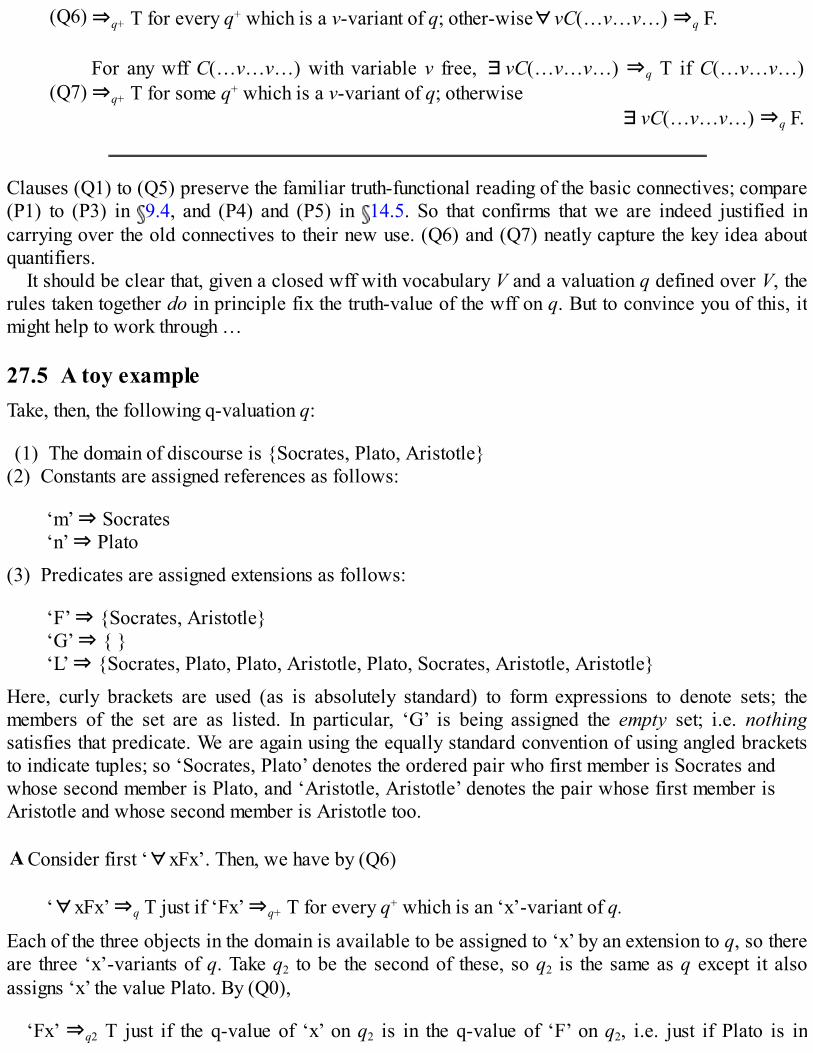
(Q6) ⇒q+ T for every q+ which is a v-variant of q; other-wise∀vC(…v…v…) ⇒q F.

(Q7)For any wff C(…v…v…) with variable v free, ∃vC(…v…v…) ⇒q T if C(…v…v…)⇒q+ T for some q+ which is a v-variant of q; otherwise

∃vC(…v…v…) ⇒q F.

Clauses (Q1) to (Q5) preserve the familiar truth-functional reading of the basic connectives; compare(P1) to (P3) in 9.4, and (P4) and (P5) in 14.5. So that confirms that we are indeed justified incarrying over the old connectives to their new use. (Q6) and (Q7) neatly capture the key idea aboutquantifiers.

It should be clear that, given a closed wff with vocabulary V and a valuation q defined over V, therules taken together do in principle fix the truth-value of the wff on q. But to convince you of this, itmight help to work through …

27.5 A toy exampleTake, then, the following q-valuation q:

(1) The domain of discourse is {Socrates, Plato, Aristotle}(2) Constants are assigned references as follows:

‘m’ ⇒ Socrates‘n’ ⇒ Plato

(3) Predicates are assigned extensions as follows:

‘F’ ⇒ {Socrates, Aristotle}‘G’ ⇒ { }‘L’ ⇒ {Socrates, Plato, Plato, Aristotle, Plato, Socrates, Aristotle, Aristotle}

Here, curly brackets are used (as is absolutely standard) to form expressions to denote sets; themembers of the set are as listed. In particular, ‘G’ is being assigned the empty set; i.e. nothingsatisfies that predicate. We are again using the equally standard convention of using angled bracketsto indicate tuples; so ‘Socrates, Plato’ denotes the ordered pair who first member is Socrates andwhose second member is Plato, and ‘Aristotle, Aristotle’ denotes the pair whose first member isAristotle and whose second member is Aristotle too.

A Consider first ‘∀xFx’. Then, we have by (Q6)

‘∀xFx’ ⇒q T just if ‘Fx’ ⇒q+ T for every q+ which is an ‘x’-variant of q.

Each of the three objects in the domain is available to be assigned to ‘x’ by an extension to q, so thereare three ‘x’-variants of q. Take q2 to be the second of these, so q2 is the same as q except it alsoassigns ‘x’ the value Plato. By (Q0),

‘Fx’ ⇒q2 T just if the q-value of ‘x’ on q2 is in the q-value of ‘F’ on q2, i.e. just if Plato is in

{Socrates, Aristotle}.

So, on q2, ‘Fx’ is false. Hence ‘∀xFx’ ⇒q F.

B Consider next ‘∀y¬(Fy ∧Gy)’. By (Q6), and then (Q1)

‘∀y¬(Fy ∧Gy)’ ⇒q T just if ‘¬(Fy ∧Gy)’ ⇒q+ T for every q+ which is a ‘y’-variant of q; i.e. justif ‘(Fy ∧Gy)’ ⇒q+ F for every q+ which is a ‘y’-variant of q.

Now consider any ‘y’-variant of q. Inspection shows that ‘(Fy ∧Gy)’ is indeed false on all of thembecause ‘Gy’ is always false. So that means ‘∀y¬(Fy ∧Gy)’ is true on q.

C Thirdly, consider ‘∀x∃yLxy’. By (Q6) again,

‘∀x∃yLxy’ ⇒q T just if ‘∃yLxy’ ⇒q+ T for every q+ which is an ‘x’-variant of q.

There are again three ‘x’-variants to consider. Take the first, q1, which assigns Socrates to ‘x’. Thenby (Q7)

‘∃yLxy’ ⇒q1 T just if ‘Lxy’ ⇒q++ T for some q++ which is a ‘y’-variant of q1.

Inspection shows that there is such an q++. Take the ‘y’-variant of q1 which assigns Plato to ‘y’. Onthis valuation, ‘Lxy’ is true, since the pair the q-value of ‘x’, the q-value of ‘y’, i.e. Socrates,Plato, is in the extension of ‘L’. So ‘ ∃yLxy’ is true on q1. Likewise, ‘∃yLxy’ comes out true on thetwo other ‘x’-variants of q. So ‘∀x∃yLxy’ ⇒q T.

These calculations are all more than a bit laborious (and just imagine if the domain had been a biggerone!). But tracking through this sort of toy example should convince you that the values of shortersubformulae – together with their values taken across families of appropriate variant valuations –will at least in principle always determine the values of more complex wffs in the intended way. Therules do indeed work as advertised!

27.6 Five results about (extended) q-valuations.In the next few chapters, we’ll invoke a number of elementary and intuitive results about (extended)q-valuations. It’s convenient to explain them here. But in fact it is enough if you read through claims(V1) to (V5) in their italicized informal versions, and are happy to accept them as intuitively true.You needn’t worry too much about the arguments which show that they are indeed true.

(V1) If a valuation makes a universal quantification true, it makes its instances true too (so longas we use names the valuation ‘knows about’). For example, suppose q is an (extended) valuationdefined over vocabulary V including the name ‘n’, and ‘∀xFx’ is true on q. Then ‘Fn’ must also betrue on q. (Proof: Let the reference of ‘n’ according to q be the object o. By assumption, ‘Fx’ is trueon every ‘x’-variant of q. So, in particular, ‘Fx’ must be true on the variant which assigns object o to‘x’. So o has to be in the extension of ‘F’. That means ‘Fn’ must be true.)

Relatedly, suppose that q is an (extended) valuation defined over vocabulary V which includes noconstants and ‘∀xFx’ is again true on q. Then there is an extension q+ of q to cover the vocabulary Vplus the new name ‘a’, such that ‘Fa’ is true on q+. (Proof: By definition there is at least one object oin the domain of q. And by assumption, ‘F’ is true of everything, so is true of o. Define q+ as q plus theassignment of o to the new name ‘a’. That will make ‘Fa’ true on q+.)

(V2) If a valuation makes an existential quantification true, it has an extension (which assigns a q-value to a new name) which makes an instance of the quantification true too. For example, supposeq is defined over vocabulary V which does not include the name ‘a’, and suppose ‘∃xFx’ is true onq. Then there is an extension q+ of q to cover the vocabulary V plus the new name ‘a’, such that ‘Fa’ istrue on q+. (Proof: By assumption, ‘Fx’ is true on some ‘x’-variant of q. So is there is some object o inthe domain that can be assigned to ‘x’ which makes ‘Fx’ true. Define q+ as q plus the assignment ofthis object o to the new name ‘a’. That will make ‘Fa’ true on q+.)

(V3) Valuations respect the equivalence between ¬∀v and ∃¬v. For example, suppose q is a an(extended) valuation which makes ‘¬∀xFx’ true. Then it makes ‘∃x¬Fx’ true. (Proof: By assumptionq must make ‘∀xFx’ false. So some ‘x’-variant of q of q makes ‘Fx’ false. So this variant makes‘¬Fx’ true. So q has an ‘x’-variant which makes ‘¬Fx’ true. So q makes ‘∃x¬Fx’ true.)

(V4) Valuations respect the equivalence between ¬∃v and ∀¬v. For example, suppose q makes‘¬∃xFx’ true. Then q makes ‘∀x¬Fx’ true. (Proof: Similar to proof for (V3).)

(V5) Extending a valuation to deal with a new constant doesn’t affect the values of wffs notcontaining that constant.(Proof: Inspection of the rules shows that when we calculate the truth-valueof a wff W on an (extended) valuation q, we only need to consider the specification of the domain,and the q-values of the names, free variables, and predicates actually in W. Suppose, for example, thename ‘a’ doesn’t appear in W; then it won’t matter what q assigns it. And if this wff W is true on someq that doesn’t evaluate ‘a’, it will remain true on an extension of q which assigns some reference tothat irrelevant name.)

Summing up, then, and putting things a little more formally:

(V1)

If an (extended) valuation q makes a wff of the form ∀vC(…v…v…) true, then (assumingq assigns a value to the constant c), q makes C(…c…c…) true. And if q doesn’t assign avalue to c, there is an extension of q to q+ which gives a q-value to c and makesC(…c…c…) true.

(V2)If q makes a wff of the form ∃vC(…v…v…) true, and c is a constant which q does notevaluate, there is an extension of q to q+ which gives a q-value to c and makesC(…c…c…) true.

(V3) If q makes a wff of the form ¬∀vC true, then it also makes true the corresponding wff ofthe form ∃v¬C.

(V4) If q makes a wff of the form ¬∃vC true, then it also makes true the corresponding wff ofthe form ∀v¬C.

(V5)Suppose q is defined over vocabulary V which doesn’t include the constant c; and supposeq+ extends q by assigning some object in the domain to c. Let W be some wff usingvocabulary from V. Then if q makes W true, so does q+.

27.7 SummaryA q-valuation defined over QL vocabulary V fixes a set of objects to be the domain of discourseD; it assigns individual constants in V objects in D as references; it assigns a truth-value to any0-place predicate in V; and when n > 0, it assigns an n-place predicate in V a (possible empty)set of n-tuples of objects in D.The key to understanding the semantics of the quantifiers is the following idea:∀vC(…v…v…)is true if C(…v…v…) would come out true, no matter which object we took v to pick out, if weregard v here as a pronoun. Simi-larly∃vC(…v…v…) is true if C(…v…v…) would come outtrue, for some possible reference for v.To implement this idea, we introduce the idea of an extended q-valuation, which assignsreferences to one or more variables as well as individual constants. Then we can say, roughly,that ∀vC(…v…v…) is true if C(…v…v…) is true no matter which object the extendedvaluation assigns to v, i.e. is true on all relevant extended valuations. And ∃vC(…v…v…) istrue if C(…v…v…) is true on some such extended valuation.Together with the natural rules for the propositional connectives, the rules for evaluatingquantified wffs ensure that a q-valuation defined over vocabulary V fixes a truth-value for anyclosed wff built up from that vocabulary.

Exercises 27Take the following q-valuation:

The domain is {Romeo, Juliet, Benedick, Beatrice}

Constants are assigned references as follows:

‘m’ ⇒ Romeo‘n’ ⇒ Juliet

Predicates are assigned extensions as follows:

‘F’ ⇒ {Romeo, Benedick}‘G’ ⇒ {Juliet, Beatrice}‘L’ ⇒ {Romeo, Juliet, Juliet, Romeo, Benedick, Beatrice,Beatrice, Benedick, Benedick, Benedick}

Then what are the truth values of the following wffs?

1. ∃x Lmx2. ∀x Lxm3 (∃x Lmx ⊃Lmn)

4. ∀x(Fx≡¬Gx)5. ∀x(Gx ⊃(Lxm ∨¬Lmx))6. ∀x(Gx ⊃∃yLxy)7. ∃x(Fx ∧∀y(Gy ⊃Lxy))

Now take the following q-valuation:

The domain is {4, 7, 8, 11, 12}

Constants are assigned references as follows:

‘m’ ⇒ 7‘n’ ⇒ 12

Predicates are assigned extensions as follows:

‘F’ ⇒ the even numbers in the domain‘G’ ⇒ the odd numbers in the domain‘L’ ⇒ the set of pairs m, n where m and n are in the domain and m is less than n

What are the truth values of the wffs (1) to (7) now?

28

Q-validity

Using the idea of a q-valuation introduced in the last chapter, we can now define the idea of a q-validargument (i.e. one whose conclusion must be true on a q-valuation if its premisses are). Unfortunately,we can’t mechanically test for q-validity in the way we can for tautological validity. But we willintroduce various ways of establishing arguments to be q-valid or q-invalid.

28.1 Q-validity definedBack in Chapter 13, we met the notion of a tautological entailment:

The PL wffs A1, A2, …, An tautologically entail the wff C if and only if there is no valuation ofthe atoms involved in the premisses Ai and the conclusion C which makes A1, A2, …, An

simultaneously all true and yet C false.

We can now introduce an analogous definition for q-entailment:

The QL closed wffs A1, A2, …, An q-entail the closed wff C if and only if there is no q-valuationof the vocabulary V involved in the premisses Ai and the conclusion C which makes A1, A2, …, An

simultaneously all true and yet C false.

Note we’ve defined q-entailment only for closed wffs – i.e. wffs with no variables dangling free, andwhich thus have determinate truth-values on a q-valuation of their vocabulary. When certainpremisses tautologically entail a conclusion we say that the inference in question is tautologicallyvalid; similarly, when a bunch of premisses q-entail a conclusion, we will say that the inference is q-valid.

Here are some more definitions:

First, if a q-valuation makes some collection of closed wffs all true, then the valuation is said tosatisfy those wffs or, equivalently, to be a model of those wffs. So another way of defining q-validity is this: an inference is q-valid just if there is no model of the premisses and negation ofthe conclusion.Second, if a q-valuation does make the premisses of some inference all true while making theconclusion false, then we will say that the valuation is a countermodel for the inference. So wecan also say: an inference is q-valid just if it has no countermodels.Third, we introduce the QL analogue of the PL notion of a tautology. A PL wff is a tautology ifit is true on all valuations of its atoms. Similarly, we will say that a closed QL wff is a q-

logical truth if it is true on all q-valuations of its vocabulary.

However, we should frankly signal that this last bit of terminology is entirely non-standard. In fact,the customary term for a q-logical truth seems to be ‘valid wff’ – which is a rather perverse bit ofnomenclature given the logician’s loud insistence elsewhere, as in 2.5, on emphaticallydistinguishing validity (a property of inferences) from truth (a feature of wffs or propositions)!

28.2 Some simple examples of q-validityTake the argument

A ∀x(Fx ⊃Gx), Fn ∴ Gn

which we might read as the QL rendition of ‘All philosophers are egocentric; Jack is a philosopher;hence Jack is egocentric’ ( 1.2, 25.1).

The inference here is certainly valid; and intuitively it is also q-valid, for it surely depends just onthe way the quantifier and the conditional works, and not on the particular interpretation of thepredicates. But how can we prove this? After all, we can’t directly check through each and everypermissible q-valuation to see what happens to the premisses and conclusion in each case: there arejust too many possibilities. The first step in specifying a q-valuation is fixing the domain ofdiscourse: but this can be any non-empty set you care to choose, however enormous. And havingchosen the domain, a one-place predicate can then have as its extension any arbitrarily selected set ofobjects from the domain. The possibilities here are literally endless. So how can we proceed?

Let’s try an indirect approach. Suppose there is a q-valuation q of the vocabulary {‘n’, ‘F’, ‘G’}which makes the premisses and the negation of the conclusion of A all true. We’ll use ‘⇒q T’ again asshorthand for ‘is T on valuation q’, dropping quotation-marks before ‘⇒’ (as we did in 16.1). Thenwe are supposing:

(1) Fn ⇒q T(2) ∃x(Fx ⊃Gx) ⇒q T(3) ¬Gn ⇒q T

At the end of the last chapter, we noted the obvious principle (V1): if the q-valuation q makes a wff ofthe form ∀vC(…v…v…) true, then q makes C(…c…c…) true, for any constant c which q evaluates.So, given (2), this principle tells us

(4) (Fn ⊃Gn) ⇒q T

Now we are in familiar territory with a familiar connective, and can continue:

But the left branch of (5) contradicts (1), and the right branch contradicts (3). Hence there can be no

such valuation q which is a countermodel to A. Which proves that the argument is indeed q-valid.For a second example, consider

B∃xFx, ∀x(Fx ⊃Gx) ∴ ∃xGx

which renders, as it might be, ‘Someone is a great logician; all great logicians are cool; hencesomeone is cool’.

Again, we need to proceed indirectly and assume for the sake of argument that there is a q-valuation q which makes the premisses true and conclusion false:

(1) ∃xFx ⇒q T(2) ∀x(Fx ⊃Gx) ⇒q T(3) ¬∃xGx ⇒q T

But if a valuation q makes ‘¬∃xGx’ true, it will make ‘∀x¬Gx’ true (as we noted in 27.6, V4). Sowe must also have

(4) ∀x¬Gx ⇒q T

Now, if a valuation q makes ‘∃xFx’ true, then some object in the domain must be in the extension of‘F’: so we can construct a q+ which extends q by assigning that object to be the referent of the newname ‘a’ ( 27.6, V2). And then

(5) Fa ⇒q+ T

What else holds on q+? If a wff not involving ‘a’ is true on a valuation q, then it remains true on anyextension q+ to deal with that constant (see 27.6, V5). So (2) implies that ∀x(Fx ⊃Gx) ⇒q+ T too;and applying (V1) again, we get

(6) (Fa ⊃Ga) ⇒q+ T

Similarly (4) implies

(7) ¬Ga ⇒q+ T

But unpacking (6) immediately generates contradictions:

There can be no q+ which makes (5) to (7) all true; hence there is no q that is a countermodel to B. Sothis argument is q-valid too.

Let’s take just one more example. Consider the inference

C (∃x(Fx ∧¬Gx) ⊃¬Gn), Gn ∴ ∀x(Fx ⊃Gx)

We again start be assuming that this is not q-valid. That is, we suppose that there is a q-valuation qsuch that:

(1) (∃x(Fx ∧¬Gx) ⊃¬Gn) ⇒q T(2) Gn ⇒q T(3) ¬∀x(Fx ⊃Gx) ⇒q T

Immediately, by (V3), we can infer

(4) ∃x¬(Fx ⊃Gx) ⇒q T

Applying to (1) the familiar rule for dealing with conditionals gives

We can apply the principle (V4) to continue the left-hand branch

(6) ∀x¬(Fx ∧¬Gx) ⇒q T

And now looking at (4), we can apply (V2) again: if a valuation q makes ‘∃x¬(Fx ⊃Gx)’ true, and‘a’ is a new constant that q doesn’t evaluate, then there must be an extension q+ of q to cover the newname ‘a’, such that

(7) ¬(Fa ⊃Ga) ⇒q+ T

We again remember that wffs not involving ‘a’ that are true on q must remain true on an extendedvaluation that assigns some object to ‘a’. That holds in particular of (6). So ‘∀x¬(Fx ∧¬Gx)’remains true on q+. And applying (V1) we get (8), and then can quickly finish:

We hit contradictions again. There can be no q+ which makes (7) and (8) both true; hence there is no q

is a countermodel to C, and so the inference is q-valid.But of course, we’ve seen trees very like these before! In fact, strip off the explicit assignments of

values and these are exactly the trees we met informally in Chapter 25 (Examples A, F, K). So whatis going on here?

28.3 Thinking about trees againRecall what we said about PL trees. We first introduced these as a way of presenting ‘workingbackwards’ arguments in English about valuations. We then dropped the explicit assignments of truth-values, for the sake of brevity. Still, the trees remained ways of presenting metalinguistic arguments.In Chapter 20, however, we pointed out that these same unsigned trees could equally well be read asobject-language arguments (i.e. arguments in PL, not arguments about PL). Read that way, theyrepresent inferences within PL, revealing the commitments of an initial bunch of assumptions. And aclosed tree shows that this bunch of assumptions is inconsistent.

In Chapter 25, we introduced QL trees. We didn’t then have the notions of a q-valuation and of q-validity to hand. So at that point, we couldn’t think of the trees metalinguistically, as arguments aboutQL valuations. We had to think of them in the second way, as representing inferences within QL, witha closed tree showing that an initial set of assumptions is inconsistent. And the tree inferences werethen justified intuitively, using an informal notion of validity.

But now we do have formal semantic notions in play. So we can now construct metalinguistic treearguments about possible q-valuations.

Looking at our three quick examples of metalinguistic trees, we see that the way they areconstructed exactly parallels the object-language arguments we met before. And the principles (V1)to (V5) of 27.6 justify analogues of the intuitive rules for the quantifiers that we adopted before. Inparticular, (V1) tells us that we can extend a tree argument about the q-valuation q by instantiating auniversal quantification with respect to a constant that q already ‘knows about’. And (V2) tells us thatif q makes an existential quantification true, then there will be an extension q+ which makes true aninstantiation of it by a new name. So we can extend a tree argument about the q-valuation q byinstantiating an existential quantification with respect to a new constant, to get something true on q+.

We will tidy up these observations in 30.1. But what they suggest is that the unsigned trees weintroduced in Chapter 25 (as arguments to establish the intuitive validity of certain QL inferences)can also be viewed as shorthand for arguments about q-valuations, with closed trees establishing notjust the validity but the q-validity of inferences.

28.4 Validity, q-validity, and ‘quantification logical form’The idea of tautological entailment captures the idea of an inferential move’s being valid by virtue ofthe distribution of the truth-functional propositional connectives among the premisses and conclusion(i.e. being valid irrespective of the meanings of the atoms the connectives connect). Similarly, theidea of q-validity captures the idea of an inference which is valid in virtue of ‘quantificational logicalform’, i.e. in virtue of the distribution of connectives and quantifiers among the premisses andconclusion (so valid irrespective of the meanings of the names and predicates that are involved in theargument).

Compare our remarks about logical form in 3.6 and 13.6. While the notion of logical form ingeneral is murky, the notion of a QL argument’s being valid in virtue of its quantificational logical

form is in perfect order and can be formally defined. It is just the notion of q-validity.An inference can be valid without being tautologically valid; and it can be valid without being q-

valid either. For example, consider the reading of QL where the domain of discourse is humans, thepredicate ‘F’ means father, and ‘G’ means male. Given those interpretations, the little argument

D∃xFx ∴ ∃xGx

is evidently valid (if there are fathers, there must be males). But it isn’t valid in virtue ofquantificational logical form. There are q-valuations of the vocabulary which make the premiss trueand the conclusion false: e.g., let the extension of ‘F’ be the set of great Cambridge philosophers, andlet the extension of ‘G’ be empty. Of course, this q-valuation doesn’t conform to the interpretation thatwe just gave ‘F’ and ‘G’. That’s allowed, though, exactly as we allowed PL truth-val-uations whichdo not respect the meanings of atoms (see 13.2). The q-valuations of wffs are intended to generateassignments of truth-values which are allowed so far as the meanings of the connectives andquantifiers are concerned.

However, although there can be arguments which are valid without being tautologically valid, wesaw that any PL argument which is tautologically valid is plain valid (see 13.2 again). Similarly,although there can be arguments which are valid without being q-valid, any QL argument which is q-valid is plain valid. Or to put it the other way about, if an argument isn’t valid, it can’t be q-valid.Why?

Take the single premiss case for simplicity (the generalization is trivial). If the inference from A toC is not valid, there must be some possible situation which would make A true and C false. But whenA and C are wffs of QL, a situation can only make A true and C false by fixing the domain andimposing certain q-values on the constituent names and predicates, since these values are all thatmatters for determining the truth-values of QL wffs. Hence if the inference from A to C is indeedinvalid, there must be a q-valuation of their vocabulary which makes A true and C false – and thatmeans that A does not q-entail C. (For a cautionary remark, however, see 34.4.)

Summing that up: q-validity stands to QL arguments as tautological validity stands to PLarguments.

28.5 The undecidability of q-validityWe saw that we can mechanically decide whether a PL argument is tautologically valid byexhaustively looking at all the possible different valuations of the atoms that occur in the argument(that’s a finite number, of course), and asking whether any valuation makes the premisses true and theconclusion false. As we remarked before, we can’t similarly test whether a QL argument is q-validby exhaustively looking at all the possible different q-valuations of the vocabulary that occur in theargument. There are just too many possibilities.

Still, although we can’t do a brute-force search through all possible q-valuations of somevocabulary, couldn’t there be some alternative mechanical method of determining whether anyargument is q-valid?

There are some special cases where there are mechanical tests: the simplest one is where all thepredicates that appear in the argument are one-place. Construct a QL tree, applying the rules as oftenas possible. Either it closes, and the argument is proved valid. Or it must terminate with no morerules left to apply (once we’ve instantiated any universal quantifier with every name in sight), but

leaving an open branch. And then we can read off a countermodel to show the argument is invalid:see 29.3.

However, as soon as there is even a single two-place predicate featuring in an argument, treesneedn’t terminate, and there won’t in general be a mechanical method for deciding q-validity. Thatresult is mathematically demonstrable. However, we can’t demonstrate it here. For a start, we wouldhave to carefully investigate the general theory of ‘mechanical methods’, which is in effect the generaltheory of what computers can do: and that is evidently a non-trivial business which would take us toofar afield. (The undecidability result belongs to a family of exciting ‘limitative’ results about what canbe done by mechanical methods, discovered in the 1930s by Kurt Gödel, Alan Turing and others.)

If we can’t in general test for q-validity by anything akin to a truth-table test, we have to resort tothe likes of tree proofs to demonstrate validity. And as we’ll see, our tree system can be beefed up tobecome a complete proof system in the sense that, if an argument is valid, we can always show it tobe valid using trees. But that point doesn’t conflict with the point about undecidability: claiming thatwe can always prove an argument is q-valid by some approved method if it is q-valid doesn’t meanthat there is a mechanical way of telling whether there is a proof or not.

In short, then, to explore the logic of QL arguments further we need to consider methods of proof,such as trees. So we return to them in the next chapter.

28.6 Countermodels and invalidityBut before moving on to consider tree proofs again, let’s consider how we might directly show that aq-invalid argument is q-invalid.

How do we do that? By finding q-valuations that work as countermodels, of course. Later, we’llsee how we can sometimes do this systematically by reading valuations off open trees ( 29.4, 30.4).Here we’ll just work very informally through a few examples.

Consider the inference:

E∀x(Fx ⊃ Hx), ∀x(Gx ⊃ Hx) ∴ ∀x(Fx ⊃ Gx)

Suppose we interpret the predicates so this translates as ‘All cats are mammals; all dogs aremammals; hence all cats are dogs’. We immediately see that E is invalid by the invalidity principle (2.3). And this interpretation can be parlayed into a formal countermodel to show the q-invalidity ofE. Just put

Domain of discourse is the set of animalsExtension of ‘F’ = the set of catsExtension of ‘G’ = the set of dogsExtension of ‘H’ = the set of mammals

and we get a q-valuation which makes the premisses true and the conclusion false.However, we just picked that counterexample/countermodel out of thin air. Can we proceed a little

bit more methodically?We are looking for a q-valuation which makes ‘∀x(Fx ⊃ Gx)’ false. That requires there to be an

object in the domain which is in the extension of ‘F’ but not in the extension of ‘G’ (why?). Let’sinsert an object into the domain to play this role – anything will do, e.g. Gwyneth Paltrow, Brad Pitt,… or the number 0. Take the latter (as it is less distracting!). And let’s try to be minimalist, and start

off with nothing else in the domain, so we’ll try to build up our q-valuation starting as follows:

Domain = {0}, i.e. the set containing just 0Extension of ‘F’ = {0}Extension of ‘G’ = { }, i.e. the empty set

This evidently makes the conclusion of E false; so far, so good. Next, to make ‘∀x(Fx ⊃ Hx)’ true,anything which is in the extension of ‘F’ must be in the extension of ‘H’ (why?). So, let’s put

Extension of ‘H’ = {0}

and the first premiss comes out true. And as it happens, that’s enough to make the second premiss truetoo. That’s because ‘∀x(Gx ⊃ Hx)’ is true on this valuation so long as ‘(Gx ⊃ Hx)’ comes out trueon every extension which assigns an object in the domain to ‘x’. The only object in the domain is 0;and ‘(Gx ⊃ Hx)’ is true when ‘x’ is treated as referring to that, since the antecedent of the conditionalwill be false and the conclusion true. Therefore our mini-model for the premisses is indeed anothercountermodel for the inference.

Take a second example:

F∀x(Fx ∨ Gx) ∴ (∀xFx ∨∀xGx)

This is q-invalid (and plain invalid for most readings of ‘F’ and ‘G’). Compare: every number is evenor odd; but it doesn’t follow that every number is even or that every number is odd. Hence, for acountermodel, suppose the domain is the set of natural numbers, the extension of ‘F’ is the evennumbers, and the extension of ‘G’ is the odd numbers.

Again, we can proceed more methodically. We are looking for a valuation which makes ‘(∀xFx∨∀xGx)’ false, i.e. makes each of ‘∀xFx’ and ‘∀xGx’ false. So there must be something in thedomain which isn’t in the extension of ‘F’ and also something in the domain which isn’t in theextension of ‘G’. Can we get a countermodel with a one-element domain? Well, if the domain is {0},then the extensions of ‘F’ and ‘G’ will have to be empty to make ‘∀xFx’ and ‘∀xGx’ false. But then‘∀x(Fx ∨ Gx)’ will be false too, so we haven’t got a countermodel.

So let’s try a two-element domain, say {0, 1}. A bit of experimenting shows that e.g.

Domain = {0, 1}Extension of ‘F’ = {0}Extension of ‘G’ = {1}

will do the trick and provide a countermodel.If we only have monadic predicates in play, things stay fairly simple (again, see 29.3). But if an

inference involves even one dyadic predicate, then we may need an infinite countermodel to showthat it is invalid. Thus consider

G ∀x∃yLxy, ∀x∀y∀z((Lxy ∧ Lyz) ⊃Lxz) ∴ ∃xLxx

Here, the first premiss says that everything stands in the relation L to something or other; and thesecond premiss says that L is a transitive relation (a relation L is transitive if when a has L to b, andb has L to c, then a has L to c: for example ‘being an ancestor of’ or ‘being taller than’ are transitive).

Now, suppose that these premisses are satisfied in a finite domain. Start from some element o1 in thedomain. Then by the first premiss, this initial element is related by L to some element o2 in thedomain, and o2 is related by L to some element o3, and so on and so forth. And if there are only afinite number of elements to choose from, we must in the end revisit some element on we’ve metbefore. In short, we will have a finite L-related chain of elements such that

o1 →o2 →… →on →on+1 →… →on

But, by the second premiss, if on is L to on+1, and on+1 is L to on+2, then on is L to on+2; and if on is L toon+2 and on+2 is L to on+3, then on is L to on+3. And so on. In other words, by the transitivity premiss, on

is L-related to everything further down the chain. So in particular, on is L-related to on itself. Whichmakes ‘∃x Lxx’ true. In short, if the premisses of G are true in a finite domain, so is the conclusion!

Yet the argument G is evidently invalid. Compare ‘Take any number, there is some number it is lessthan; if a number is less than a second number, and the second is less than a third, then the first is lessthan the third; hence there is a number which is less than itself’, which has true premiss and a falseconclusion. That’s a counterexample to the validity of G, and the corresponding infinite countermodelis

Domain = {0, 1, 2, …}, i.e. the infinite set of all positive integersExtension of ‘L’ = the set of pairs m, n such that m < n.

28.7 SummaryA q-valid inference is a QL inference which is such that, on any q-valuation of the vocabulary Vin the premisses and the conclusion, if the premisses are all true together, the conclusion is truetoo.There is no generally applicable mechanical method for determining whether an argument is q-valid (contrast the truth-table test for mechanically settling the tautological validity of PLarguments).We can establish a q-valid argument to be q-valid by showing that the idea that there is acountermodel (a q-valuation which makes the premisses true and conclusion false) leads tocontradiction. Such a proof is again naturally set out as a tree.We can establish a q-invalid argument to be q-invalid if we can find a countermodel. But in thegeneral case, countermodels may need infinite domains.

Exercises 28A Let’s use ‘ ’ now to abbreviate ‘q-entails’ (compare 13.7). Which of the following claims are

true? Provide arguments in the style of 28.2 and 28.6 to defend your answers.

1. ∀x(Fx ⊃Gx) ∀x(Gx ⊃Fx)2. ∀x(Fx ⊃Gx) ∀x(¬Gx ⊃¬Fx)3. ∀x∃yLxy ∀y∃xLyx4. ∀x((Fx ∧Gx) ⊃Hx) ∀x(Fx ⊃(Gx ⊃Hx))5. (∀xFx ∨∀xGx) ∀x(Fx ∨Gx)6. ∀x(Fx ⊃Gx), ∀x(¬Gx ⊃Hx) ∀x(Fx ⊃¬Hx)

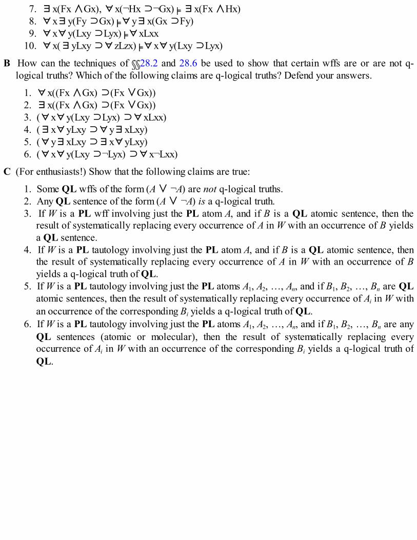
7. ∃x(Fx ∧Gx), ∀x(¬Hx ⊃¬Gx) ∃x(Fx ∧Hx)8. ∀x∃y(Fy ⊃Gx) ∀y∃x(Gx ⊃Fy)9. ∀x∀y(Lxy ⊃Lyx) ∀xLxx

10. ∀x(∃yLxy ⊃∀zLzx) ∀x∀y(Lxy ⊃Lyx)

B How can the techniques of 28.2 and 28.6 be used to show that certain wffs are or are not q-logical truths? Which of the following claims are q-logical truths? Defend your answers.

1. ∀x((Fx ∧Gx) ⊃(Fx ∨Gx))2. ∃x((Fx ∧Gx) ⊃(Fx ∨Gx))3. (∀x∀y(Lxy ⊃Lyx) ⊃∀xLxx)4. (∃x∀yLxy ⊃∀y∃xLxy)5. (∀y∃xLxy ⊃∃x∀yLxy)6. (∀x∀y(Lxy ⊃¬Lyx) ⊃∀x¬Lxx)

C (For enthusiasts!) Show that the following claims are true:

1. Some QL wffs of the form (A ∨ ¬A) are not q-logical truths.2. Any QL sentence of the form (A ∨ ¬A) is a q-logical truth.3. If W is a PL wff involving just the PL atom A, and if B is a QL atomic sentence, then the

result of systematically replacing every occurrence of A in W with an occurrence of B yieldsa QL sentence.

4. If W is a PL tautology involving just the PL atom A, and if B is a QL atomic sentence, thenthe result of systematically replacing every occurrence of A in W with an occurrence of Byields a q-logical truth of QL.

5. If W is a PL tautology involving just the PL atoms A1, A2, …, An, and if B1, B2, …, Bn are QLatomic sentences, then the result of systematically replacing every occurrence of Ai in W withan occurrence of the corresponding Bi yields a q-logical truth of QL.

6. If W is a PL tautology involving just the PL atoms A1, A2, …, An, and if B1, B2, …, Bn are anyQL sentences (atomic or molecular), then the result of systematically replacing everyoccurrence of Ai in W with an occurrence of the corresponding Bi yields a q-logical truth ofQL.

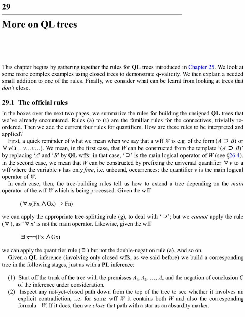
29

More on QL trees

This chapter begins by gathering together the rules for QL trees introduced in Chapter 25. We look atsome more complex examples using closed trees to demonstrate q-validity. We then explain a neededsmall addition to one of the rules. Finally, we consider what can be learnt from looking at trees thatdon’t close.

29.1 The official rulesIn the boxes over the next two pages, we summarize the rules for building the unsigned QL trees thatwe’ve already encountered. Rules (a) to (i) are the familiar rules for the connectives, trivially re-ordered. Then we add the current four rules for quantifiers. How are these rules to be interpreted andapplied?

First, a quick reminder of what we mean when we say that a wff W is e.g. of the form (A ⊃ B) or∀vC(…v…v…). We mean, in the first case, that W can be constructed from the template ‘(A ⊃ B)’by replacing ‘A’ and ‘B’ by QL wffs: in that case, ‘⊃’ is the main logical operator of W (see 26.4).In the second case, we mean that W can be constructed by prefixing the universal quantifier ∀v to awff where the variable v has only free, i.e. unbound, occurrences: the quantifier v is the main logicaloperator of W.

In each case, then, the tree-building rules tell us how to extend a tree depending on the mainoperator of the wff W which is being processed. Given the wff

(∀x(Fx ∧Gx) ⊃ Fn)

we can apply the appropriate tree-splitting rule (g), to deal with ‘⊃’; but we cannot apply the rule(∀), as ‘∀x’ is not the main operator. Likewise, given the wff

∃x¬¬(Fx ∧Gx)

we can apply the quantifier rule (∃) but not the double-negation rule (a). And so on.Given a QL inference (involving only closed wffs, as we said before) we build a corresponding

tree in the following stages, just as with a PL inference:

(1) Start off the trunk of the tree with the premisses A1, A2, …, An and the negation of conclusion Cof the inference under consideration.

(2) Inspect any not-yet-closed path down from the top of the tree to see whether it involves anexplicit contradiction, i.e. for some wff W it contains both W and also the correspondingformula ¬W. If it does, then we close that path with a star as an absurdity marker.

(3) If we have run out of rules to apply to unchecked non-primitive formulae left on any open path,then we have to stop!

(4) Otherwise, we choose some unchecked non-primitive formula W that sits on an open path. Wethen apply the appropriate rule, and extend the tree by adding more (closed) wffs in thedescribed way. We can then check off W, except after an application of rule (∀).

(5) Loop back to step (2).

Rules for building QL trees*

Suppose that W is a non-primitive wff on an open branch. We can then apply the corresponding rule:

(a) W is of the form ¬¬A: add A to each open path containing W. Check off W. Schematically,

(b) W is of the form (A ∧ B): add both A and B to each open path containing W. Check off W.(c) W is of the form ¬(A ∨ B): add ¬A and ¬B to each open path containing W. Check off W.(d) W is of the form ¬(A ⊃ B): add A and ¬B to each open path containing W. Check off W.

(e) W is of the form (A ∨ B): add a new fork to each open path containing W, with branches leadingto the alternatives A and B. Check off W.

(f) W is of the form ¬(A ∧ B): add a new fork to each open path containing W, with branchesleading to the alternatives ¬A and ¬B. Check off W.

(g) W is of the form (A ⊃ B): add a new fork to each open path containing W, with branches leadingto the alternatives ¬A and B. Check off W.

(h) W is of the form (A ≡ B): add a new fork to each open path containing W, leading to thealternatives A, B and ¬A, ¬B. Check off W.

(i) W is of the form ¬(A ≡ B): add a new fork to each open path containing W, leading to thealternatives A, ¬B and ¬A, B. Check off W.

(¬∀) W is of the form ¬∀vC: add ∃v¬C to each open path on which W appears. Check off W.(¬∃) W is of the form ¬∃vC: add ∀v¬C to each open path on which W appears. Check off W.

(∀) W is of the form ∀vC(…v…v…): add C(…c…c…) to an open path on which W appears,where c is a constant on that path (which hasn’t already been used to instantiate W on that path).W is not checked off.

(∃) W is of the form ∃vC(…v…v…): add C(…c…c…) to each open path on which W appears,where c is a constant new to the paths. Check off W.

As we saw ( 25.5), this process may not terminate in the case of QL trees – and it is possible forinjudicious choices at step (4) of the tree-building process to lead to a non-terminating tree eventhough other choices would lead to a closed tree.

Why do we check off a wff W when we apply the appropriate tree-building rule, except when W isuniversally quantified wff and we are applying the (∀) rule? Because in the other cases, theunpacking rules effectively exhaust the content of the wff we are unpacking (and there is no point indoing that twice over). By contrast, a universal quantified wff tells us that everything in the domainsatisfies a certain condition. We can of course infer that a particular named object in the domainsatisfies that condition. But there is more content to the original quantified claim than is given by thatparticular implication of it.

And why does the (∀) rule tell us not to re-instantiate a universally quantified wff using the sameconstant again on the same path? Because that would be quite redundant. It would just put a duplicateof the same wff on the same path.

29.2 Further examples of closed treesLet’s consider more inferences involving wffs with multiple quantifiers. Take first:

A Some people are boastful. No one likes anyone boastful. So some people aren’t likedby anyone.

To confirm the argument is valid, translate it into QL, e.g. by

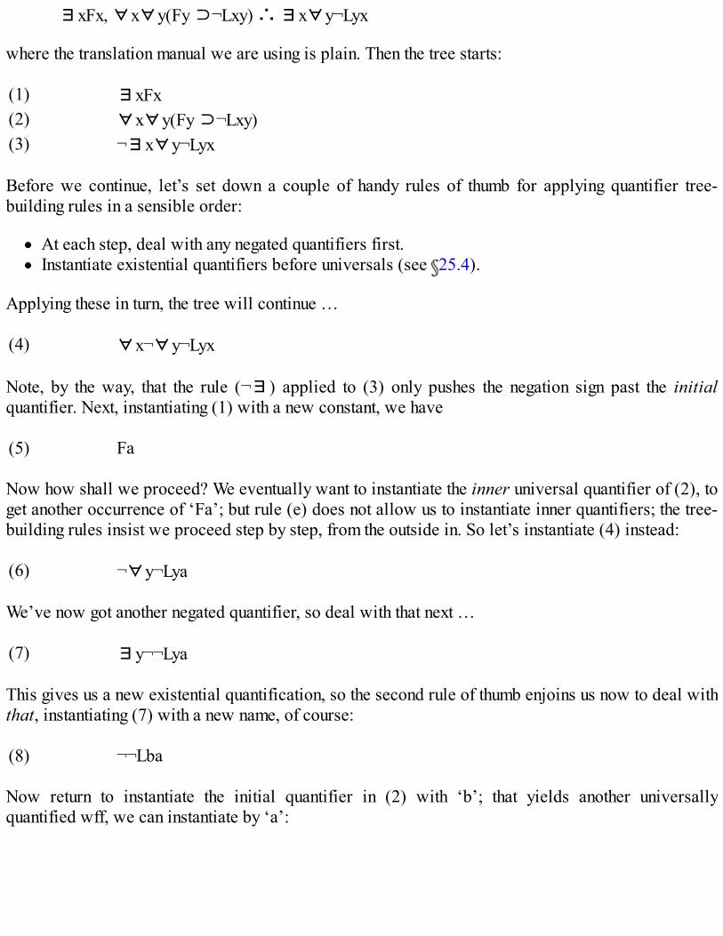
∃xFx, ∀x∀y(Fy ⊃¬Lxy) ∴ ∃x∀y¬Lyx

where the translation manual we are using is plain. Then the tree starts:

(1) ∃xFx(2) ∀x∀y(Fy ⊃¬Lxy)(3) ¬∃x∀y¬Lyx

Before we continue, let’s set down a couple of handy rules of thumb for applying quantifier tree-building rules in a sensible order:

At each step, deal with any negated quantifiers first.Instantiate existential quantifiers before universals (see 25.4).

Applying these in turn, the tree will continue …

(4) ∀x¬∀y¬Lyx

Note, by the way, that the rule (¬∃) applied to (3) only pushes the negation sign past the initialquantifier. Next, instantiating (1) with a new constant, we have

(5) Fa

Now how shall we proceed? We eventually want to instantiate the inner universal quantifier of (2), toget another occurrence of ‘Fa’; but rule (e) does not allow us to instantiate inner quantifiers; the tree-building rules insist we proceed step by step, from the outside in. So let’s instantiate (4) instead:

(6) ¬∀y¬Lya

We’ve now got another negated quantifier, so deal with that next …

(7) ∃y¬¬Lya

This gives us a new existential quantification, so the second rule of thumb enjoins us now to deal withthat, instantiating (7) with a new name, of course:

(8) ¬¬Lba

Now return to instantiate the initial quantifier in (2) with ‘b’; that yields another universallyquantified wff, we can instantiate by ‘a’:

And we are done. The inference is q-valid, and hence valid. (Make sure you see why it was sensibleto instantiate (2) with ‘b’ rather than ‘a’.)

Consider next

B Everyone admires some logician; whoever admires someone respects them. Soeveryone respects some logician.

The translation of the premisses and negated conclusion shouldn’t cause trouble by now (just note thatthe second premiss means that for any pair, if the first admires the second, then the first respects thesecond):

(1) ∀x∃y(Fy ∧Lxy)(2) ∀x∀y(Lxy ⊃ Mxy)(3) ¬∀x∃y(Fy ∧Mxy)

Checking off (3), the next steps are more or less automatic.

We could instantiate (6) using ‘a’, but that would be pointless. So let’s next instantiate (1) and (2)instead:

(7) ∃y(Fy ∧Lay)(8) ∀y(Lay ⊃ May)

Next, instantiating the existential quantification first (following our rule of thumb), and rememberingto use a new constant, we get

(9) (Fb ∧Lab)

Using this new constant to instantiate the two remaining universal quantifiers at (6) and (8), we get

(10) ¬(Fb ∧Mab)(11) (Lab ⊃ Mab)

Finally the tree closes using the familiar connective rules:

Let’s next revisit an example from 5.4:

C No girl loves any sexist pig. Caroline is a girl who loves whoever loves her; Henryloves Caroline; hence Henry is not a sexist pig.

Rendered into QL using an obvious translation dictionary, the tree will start:(1) ∀x(Gx ⊃¬∃y(Fy ∧Lxy))(2) (Gm ∧∀x(Lxm ⊃Lmx))(3) Lnm(4) ¬¬Fn

And the next few steps are straightforward. Just unpack the conjunction in (2), checking it off, andthen instantiate (1) with respect to ‘m’:

That leaves us with two universal quantifications, at (6) and (9), to instantiate. Instantiating (9) by ‘n’will give us ‘Fn’ in the scope of a negation, which should contradict the earlier ‘¬¬Fn’. And it does…

The obvious thing to do now is to instantiate (6) with respect to ‘n’ as well, to conclude the tree

We are done: the inference is valid.Our fourth sample argument is of a type which was recognized by medieval logicians as being

valid, but couldn’t be shown to be so within their logic of general propositions:

D All horses are mammals; so any horse’s head is a mammal’s head.

Modern logicians can do better than their predecessors here. In fact, as soon as we see how totranslate the conclusion into QL, finding a tree to show that D is indeed q-valid is straightforward.

First, then, the translational problem. ‘Any horse’s head is a mammal’s head’ is equivalent to ‘Forany x, if x is the head of some horse, then x is the head of some mammal’, i.e. ‘for any x, if (for somehorse y, x is the head of y), then (for some mammal z, x is the head of z)’. So, let’s fix on thedictionary

‘F’ means … is a horse‘G’ means … is a mammal‘M’ means … is the head of …

and set the domain to be e.g. earthly things. Then C’s conclusion can be rendered

x{∃y(Fy ∧Mxy) ⊃∃z(Gz ∧Mxz)}

The tree will therefore commence

That’s pretty much automatic given our two rules of thumb for tree-building. We dealt first with thenegated quantifier at (2) to give (3). That leaves us with the universally quantified (1) and theexistentially quantified (3), so we apply the ‘existentials before universals’ rule. Stripping off thequantifier ‘∃x’, and replacing every occurrence of ‘x’ with a new name gives us (4). Note thebracketing in (4); it is a negated conditional. So applying the relevant rule gives us (5) and (6). Again,we first deal with the negated quantifier, and check off (6) to yield

Now we have two universally quantified propositions at (1) and (7), and the existential quantificationat (5). So next instantiate (5) with a new name:

and then the rest is straightforward. Instantiating (1) and (7) with respect to ‘b’ (why try ‘b’ ratherthan ‘a’?), and then unpacking the connectives, we finish …

Finally in this section, we’ll return to 5.1, and again consider

E Everyone loves a lover; Romeo loves Juliet; so everyone loves Juliet.

We saw that this is valid if the first premiss is interpreted to mean ‘everyone loves anyone who is alover’ (i.e. ‘everyone x is such that, take anyone y, if y loves someone then x loves y’). Using ‘L’ forloves, etc., we begin the tree

(1) ∀x∀y(∃z Lyz ⊃Lxy)(2) Lmn(3) ¬∀xLxn

Following the rule of thumb ‘negated quantifiers first’, we can check off (3) and add:

(4) ∃x¬Lxn

Remembering the other tip, ‘existentials before universals’, we instantiate (4):

(5) ¬Lan

But now what? Let’s try instantiating the two quantifiers in (1) – one at a time! – with ‘a’ and ‘n’,which will make the consequent of the conditional ‘Lan’, preparing the way for a contradiction with(5). So we get

How do we carry on from here? Consider the argument we gave to show that this inference is valid in5.1. We in fact had to use the first premiss twice there, at lines (4) and (7) of the informal proof. We

might expect to have to use the premiss twice to close off this tree. So let’s press on, and instantiate(1) again

With a bit of effort, again we are done. The inference E is q-valid (and so valid).It’s worth pausing just a moment to compare this last demonstration of validity with the simple

informal proof in 5.1. Evidently, the tree proof is a lot less ‘natural’ and direct than the informal one.But remember: trees are not being sold as the best way of formally mimicking ordinary styles of

deduction (cf. 20.3): they are not a ‘natural deduction’ proof system. All that is being claimed is thattrees are one well-motivated and reasonably manageable way of showing that inferences are q-validwhen they are.

For yet more examples of our tree-rules at work, see Chapter 35.

29.3 Extending the (∀) ruleAs we noted before ( 28.3), our stated rules for tree-building certainly look sound (i.e. an argumentwarranted by a closed tree built following our rules is indeed q-valid). If we start a tree by assumingthat A1, A2, …, An, ¬C are all true on some valuation q, then the quantifier rules for extending the treeare warranted by the principles (V1) to (V5) about valuations ( 27.6). Hence, if the tree does end upin contradictions, there can be no such valuation q; and then the target inference A1, A2, …, An ∴ Cmust be q-valid. We’ll turn this rough and ready proof-idea into a tidier affair in the next chapter.

But is our basic set of rules complete (i.e. do we have enough tree-building rules to find a closedtree corresponding to every q-valid inference)?

Consider the inference ‘∀xFx ∴ ∃xFx’. If we try to construct a tree, we’ll get as far as

Then we have to stop, as there is no further rule to apply. So the tree doesn’t close. On the other hand,the inference is q-valid according to our account. Take any q-valuation q. If q makes ‘∀xFx’ true,then every object in q’s domain needs to be in the extension of ‘F’. Since domains are non-empty, thatmeans at least one thing is in the extension of ‘F’. So q must make ‘∃xFx’ true too.

Now, this last point only holds because we chose to say that domains always have at least onemember ( 27.2). Suppose we’d taken the other tack and allowed empty domains. Then ‘∀xFx ∴∃xFx’ would no longer be q-valid. Given an empty domain it is vacuously true that, if any object isin the domain, it is in the extension of ‘F’ (that’s a general conditional claim with an antecedent whichis always false). So ‘∀xFx’ is true in an empty domain. But ‘∃xFx’ will be false.

In sum, our tree-rules are currently out of harmony with our definition of q-validity. Our rules don’twarrant the inference ‘∀xFx ∴ ∃xFx’; our definition of q-validity does. What to do?

There is a forking of the paths here. You might think the obvious response is to backtrack hastily,revise our definition of validity, adopting instead the idea of q0-validity (defined in terms of q0-valuations, which are exactly like q-valuations except that they allow empty domains). And if we dothat, it can be proved that our current set of rules would then be complete. There are closed treesusing our existing rules for all and only the q0-valid arguments. So that looks like a happy restorationof harmony. Unfortunately, there is a snag.

Consider the inferences ‘∀xFx ∴ Fn’ and ‘Fn ∴ ∃xFx’. These are both straightforwardly q0-valid (take any valuation of the vocabulary in the premisses and conclusion: that will involveassigning an object as q-value to ‘n’; so these valuations won’t have empty domains). Then we have‘∀xFx ∴ Fn’ and ‘Fn ∴ ∃xFx’ are q0-valid and ‘∀xFx ∴ ∃xFx’ isn’t. Or putting it more starkly,we have A q0-entails B, B q0-entails C, but A does not q0-entail C. Which goes clean against ournormal assumption that entailments can be chained into longer arguments and our ultimate conclusionwill still follow from our initial premiss(es). What to do?

Well, we could adopt a notion of entailment which allows exceptions to that fundamentalassumption. Or we could be revisionary in another way and reject ‘∀xFx ∴ Fn’ as a validentailment in the absence of an explicit premiss to the effect ‘n exists’. But most logicians prefer tostick to the two assumptions that we can unrestrictedly chain entailments and endorse ‘∀xFx ∴ Fn’.

We are going to follow the majority here (though see Chapter 36 for some more comments). Hencewe shall not revise our definition of q-validity to allow empty domains. That means ‘∀xFx ∴∃xFx’ remains q-valid. It also means, however, that we need a further tree-building rule if we are tobe able to warrant every q-valid argument by means of a closed tree.

One popular option here is to relax the rule (∀) rather radically. The rule currently says that if Wis of the form ∀vC(…v…v…), then we can add C(…c…c…) to any open path on which W appears,where c is a constant already on the path. Suppose instead that we are allowed to instantiate W withany constant, old or new. Then we can close the tree which we had trouble with before:

Here we’ve just arbitrarily chosen to use the constant ‘c0’. Since we are assuming that there is at leastone thing in the domain, pick such an object, and we can surely use a new name to dub it. Instantiatingthe universal quantifications at (1) and (3) with a name of this object then exposes a contradiction.

But our suggested generous rule rather ruins the memorable symmetry between our rules (∀) and(∃), summed up in the slogan ‘instantiate universals with old constants, existentials with new ones’.There’s something unattractive too about relaxing (∀) to allow us to instantiate universals with anyconstant, and then immediately having to issue the warning that you’d be daft ever to instantiate auniversal with a random constant except in the very special circumstances that there are no otherconstants in sight to play with.

So rather than go too radical, here’s our preferred revision of the rule (∀). We’ll keep the old rulefor when there are constants already on the relevant path, and just add a clause to deal with thespecial case when we want to instantiate a universal quantification and there are no precedingconstants:

(∀′)

W is of the form ∀vC(…v…v…): add C(…c…c…) to an open path on which W appears,where c is a either a constant on that path (and which hasn’t been used to instantiate Wbefore), or is a new constant (and there are no other constants appearing on the path). W isnot checked off.

NB: Rule (∀′) still allows us to construct our mini-tree warranting ‘∀xFx ∴ ∃xFx’.We will show in the next chapter that this minor extension of our original rule does indeed give us

a sound and complete set of rules. So for the rest of this book, we’ll assume the revised rule (∀′) isin play.

29.4 What can be learnt from open trees?We have emphasized before that the fact that a quantifier tree doesn’t close doesn’t always show theargument under consideration is invalid. An injudicious sequence of choices of the rules to apply canmean that a trees trails off down an infinite path, when better choices would close off the tree (see 25.5 again).

However, in simple cases, a tree can terminate with no more rules left to apply, but leaving an openbranch. If there is an open branch on such a completed tree, then we can read off from the tree a q-valuation which makes the premisses true and conclusion false and which thus demonstrates q-invalidity. Consider, for example,

E ∀x(Fx ⊃ Hx), ∀x(Gx ⊃ Hx) ∴ ∀x(Fx ⊃ Gx)

Starting in the obvious way, and omitting the unofficial line numbers, we get:

The tree has open branches. The only unchecked wffs which aren’t atomic wffs or negations of atomicwffs are the universal quantifications at the top of the tree. But we have no new names available toinstantiate them with. So we can’t use the (∀′) rule again. There are no more rules to apply.

In the case of PL trees, if a branch stays open, we can read off a valuation which makes all thewffs on the branch true. The trick is to pick a valuation which makes the primitives on the branch,i.e. the atoms and negated atoms, all true. Then truth percolates up the branch. That makes the initialpremisses and negated conclusion all true, and the valuation therefore shows that the inference isinvalid (cf. 16.2, 19.2). Let’s try the very same trick here.

In the present case, it doesn’t matter which open branch we choose, the primitives on the branchare ‘Fa’, ‘¬Ga’, and ‘Ha’. We need to choose a reference for the name ‘a’. Let’s assign it the firstnumber, i.e., 0. And then, to give the primitives the right values, we need the extensions of ‘F’ and ‘H’to include 0, and the extension of ‘G’ not to include 0.

A domain must of course always contain any named objects and/or objects which are involved inthe extension of predicates. So in the present case, we know the domain must contain at least 0. Whatelse should we put in the domain? Nothing. We don’t want any extra objects in the domain which wehaven’t any information about (and which might therefore have unwanted effects on the truth-values ofquantified wffs). So, keeping the domain as small as possible, we get:

Domain = {0}, i.e. the set containing just 0.Reference of ‘a’ = 0.Extension of ‘F’ = extension of ‘H’ = {0}.Extension of ‘G’ = { }, i.e. the empty set.

This makes the primitives all true. And it is readily checked that this indeed makes all the wffs on anopen branch of our tree true; and in particular, it makes the premisses of E true and conclusion false(compare the discussion of the same argument in 28.5).

Here’s another example:

F ∀x(Fx ∨ Gx), ∀x(Gx ⊃ Hx) ∴ (∀xFx ∨∀xHx)

Using our rules of thumb, we get the following (again omitting line numbers):

Here, the initial steps are pretty automatic. Then we instantiate the two universal quantifications withevery name in sight, and unpack the resulting wffs. There are no more rules to apply, and the tree staysopen. So let’s try to construct a countervaluation for the argument. Take the open path, where we have

¬Fa, Fb, Ga, ¬Gb, Ha, ¬Hb

There are two names here to which we need to assign q-values. Let’s take them in order to refer to thefirst two numbers. Again we take the domain of discourse to be no larger than it needs to be toinclude those references for the names. The resulting valuation which makes the primitives all true isthen:

Domain = {0, 1}Reference of ‘a’ = 0Reference of ‘b’ = 1Extension of ‘F’ = {1}

Extension of ‘G’ = {0}Extension of ‘H’ = {0}

It is easily checked again that this valuation makes all the wffs on the open branches true. Inparticular, it makes the premisses of F true and conclusion false. Why does it make, e.g., the universalquantification (1) true? Because it makes an instance true for each object in the domain (to emphasize,there are no more objects in the domain than the named ones).

When does this trick work, i.e. this trick of reading valuations from the primitives on an openbranch on a QL tree and arriving at a countervaluation for the argument in question? For a start, itworks for arguments where the propositions don’t feature quantifiers embedded one inside the other.Instantiate all the existential quantifiers, thereby introducing a collection of new names; instantiate allthe universal quantifications with respect to all the names thereby introduced (plus any others in theoriginal premisses and conclusion). And if the tree doesn’t close, construct the ‘smallest domain’valuation which contains one object per name and which makes the primitives on some open branchtrue, and you’ll get the desired countermodel.

We saw, however, that when an argument involves embedded quantifiers life gets morecomplicated. It may be the case that the only countermodels which show that the inference is invalidare infinite ones; see the discussion of 28.5 G. Yet it may also be the case that, when we do find aninfinite branch that never closes, it doesn’t show that the argument is invalid, and we can’t read off agenuine countervaluation from the branch; see again the discussion of the example in 25.5. Lookingmore closely at the infinite open branch in that last case, we see that it in fact was constructed byignoring its lines (3) and (5). No surprise then that choosing a valuation that makes all the primitiveson that branch true won’t make (3) and (5) true too! We can only form countermodels from infinitebranches when the trees have been constructed more systematically, without ignoring any complexwffs on an open branch; but that’s not entirely straightforward (more on this in the next chapter).

29.5 SummaryWe summarized our original set of tree-building rules for quantifier trees, and argued for amodification of the rule (∀) to match our restriction to non-empty domains.A couple of useful heuristic tips – not strict rules, but guides for applying the rules in a sensibleorder: eliminate negated quantifiers first and then instantiate existentials before universals.In some simple cases at any rate, we can read countervaluations from open trees (choose a‘smallest domain’ interpretation that makes the primitives on an open branch true).

Exercises 29A Use QL trees to evaluate the entailment claims (1) to (10) in Exercises 28A.

B Using trees, show the following arguments are valid:

1. Some philosophers admire Jacques. No one who admires Jacques is a good logician. Sosome philosophers are not good logicians.

2. Some philosophy students admire all logicians; no philosophy student admires any rottenlecturer; hence, no logician is a rotten lecturer.

3. There’s a town to which all roads lead. So all roads lead to a town.4. Some good philosophers admire Frank; all wise people admire any good philosopher; Frank

is wise; hence there is someone who both admires and is admired by Frank.5. Any true philosopher admires some logician. Some students admire only existentialists. No

existentialists are logicians. Therefore not all students are true philosophers.6. Everyone loves a lover; hence if someone is a lover, everyone loves everyone!7. If anyone speaks to anyone, then someone introduces them; no one introduces anyone to

anyone unless they know them both; everyone speaks to Frank; therefore everyone isintroduced to Frank by someone who knows him. [Use ‘Rxyz’ to render ‘x introduces y toz’.]

8. Any elephant weighs more than any horse. Some horse weighs more than any donkey. If a firstthing weighs more than a second thing, and the second thing weighs more than a third, then thefirst weighs more than the third. Hence any elephant weighs more than any donkey.

C Redo the first three examples of 29.2 as signed trees (as in 28.2).

* But NB the extended version of the (∀) rule in 29.3!

30

QL trees vindicated

In this chapter, we prove the ‘Basic Result’ about QL trees: there is a closed QL tree for an argumentif and only if the inference is q-valid. Like Chapter 19, this can certainly be skipped by those with notaste for abstract metalogical argument. Still, the Basic Result is often located the other side of thethreshold that divides elementary logic from the serious stuff. So it is nice to show that the workwe’ve already done in fact allows us to give a fairly painless proof.

30.1 Soundness(Revision homework: re-read 19.1, 20.4, 27.4, 27.6, 28.2, 28.3!)

We first need to show that QL tree proofs are sound, i.e. reliable. If a properly constructed QLtree closes, then the argument under scrutiny is indeed q-valid. That’s equivalent to saying

(S) If an inference is not q-valid, then a corresponding QL tree will never close.

A quick reminder: we will say that a path through a tree is satisfiable if there is a q-valuationwhich makes all the wffs on the path true. A satisfiable path plainly cannot contain contradictory wffs,so can’t close.

Proof of (S) Suppose that the inference A1, A2, …, An ∴ C is not q-valid. Then there is somevaluation q which ensures that

A1 ⇒q T, A2 ⇒q T, …, An ⇒q T, ¬C ⇒q T

and the initial ‘trunk’ of the corresponding tree is satisfiable. Now consider what happens as weextend our tree, step by step, applying the tree-building rules. At each stage, a satisfiable path willget extended to a longer satisfiable path. So a tree with a satisfiable trunk will never close. To show that a satisfiable path always gets extended to a longer satisfiable path, we just have toinspect the building rules one at a time. It is easy to see that the result holds for the rules telling ushow to unpack wffs whose main logical operator is one of the connectives (compare 19.1). Take, forexample, the non-branching rule that unpacks a wff (A ∧ B) into its conjuncts. A q-valuation q whichsatisfies a path including (A ∧ B) will of course continue to satisfy the path we get by adding A andB, since q will make both these added new wffs true as well. Or take, for another example, thebranching rule which tells us to extend a path containing (A ∨B) by adding a fork with A on onebranch and B on the other. If q satisfies a path including (A ∨B) then at least one of A and B must betrue on q, hence q will continue to satisfy at least one of the extended paths. You can easily check thatthe same is true for extensions by means of other connective rules. Next, suppose q satisfies a path including a wff of the form ¬∀vC; then applying the relevant rule

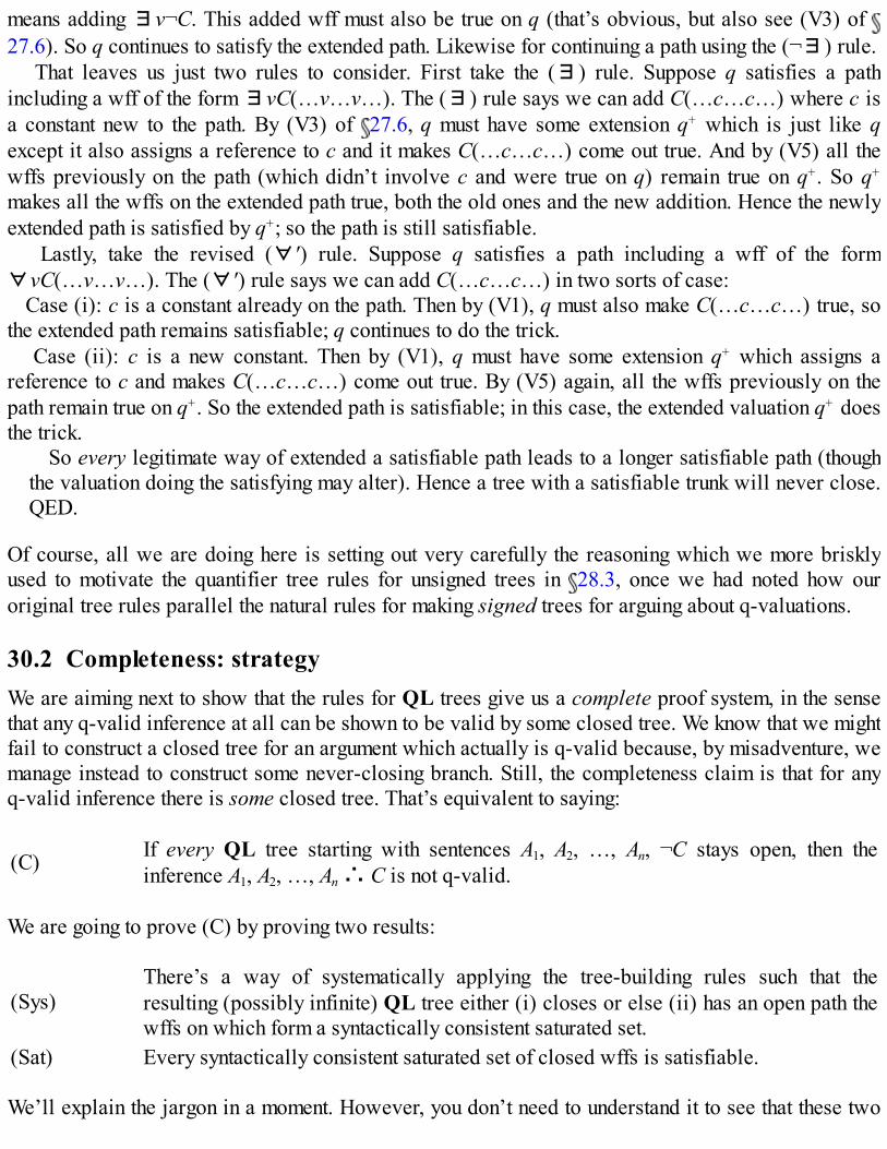
means adding ∃v¬C. This added wff must also be true on q (that’s obvious, but also see (V3) of 27.6). So q continues to satisfy the extended path. Likewise for continuing a path using the (¬∃) rule. That leaves us just two rules to consider. First take the (∃) rule. Suppose q satisfies a pathincluding a wff of the form ∃vC(…v…v…). The (∃) rule says we can add C(…c…c…) where c isa constant new to the path. By (V3) of 27.6, q must have some extension q+ which is just like qexcept it also assigns a reference to c and it makes C(…c…c…) come out true. And by (V5) all thewffs previously on the path (which didn’t involve c and were true on q) remain true on q+. So q+

makes all the wffs on the extended path true, both the old ones and the new addition. Hence the newlyextended path is satisfied by q+; so the path is still satisfiable. Lastly, take the revised (∀′) rule. Suppose q satisfies a path including a wff of the form∀vC(…v…v…). The (∀′) rule says we can add C(…c…c…) in two sorts of case: Case (i): c is a constant already on the path. Then by (V1), q must also make C(…c…c…) true, sothe extended path remains satisfiable; q continues to do the trick. Case (ii): c is a new constant. Then by (V1), q must have some extension q+ which assigns areference to c and makes C(…c…c…) come out true. By (V5) again, all the wffs previously on thepath remain true on q+. So the extended path is satisfiable; in this case, the extended valuation q+ doesthe trick.

So every legitimate way of extended a satisfiable path leads to a longer satisfiable path (thoughthe valuation doing the satisfying may alter). Hence a tree with a satisfiable trunk will never close.QED.

Of course, all we are doing here is setting out very carefully the reasoning which we more brisklyused to motivate the quantifier tree rules for unsigned trees in 28.3, once we had noted how ouroriginal tree rules parallel the natural rules for making signed trees for arguing about q-valuations.

30.2 Completeness: strategyWe are aiming next to show that the rules for QL trees give us a complete proof system, in the sensethat any q-valid inference at all can be shown to be valid by some closed tree. We know that we mightfail to construct a closed tree for an argument which actually is q-valid because, by misadventure, wemanage instead to construct some never-closing branch. Still, the completeness claim is that for anyq-valid inference there is some closed tree. That’s equivalent to saying:

(C) If every QL tree starting with sentences A1, A2, …, An, ¬C stays open, then theinference A1, A2, …, An ∴ C is not q-valid.

We are going to prove (C) by proving two results:

(Sys)There’s a way of systematically applying the tree-building rules such that theresulting (possibly infinite) QL tree either (i) closes or else (ii) has an open path thewffs on which form a syntactically consistent saturated set.

(Sat) Every syntactically consistent saturated set of closed wffs is satisfiable.

We’ll explain the jargon in a moment. However, you don’t need to understand it to see that these two

results will give us exactly what we want. If every possible tree starting from the sentences A1, A2, …,An, ¬C stays open, then by (Sys) there must in particular be a systematically built tree which has anopen path, the wffs on which form a consistent saturated set (the wffs are closed sentences, as on anylegal tree). By (Sat) there is a q-valuation which makes all the wffs in that set true. This q-valuationin particular makes all of the trunk A1, A2, …, An, ¬C true. So the inference A1, A2, …, An ∴ C is not q-valid. QED.

So to establish (C), we’ll prove (Sat) in the next section, and (Sys) in 30.4.

30.3 Consistent, saturated sets are satisfiable(Further revision homework: re-read 19.2, 19.3!)

As before, we’ll say that a set of wffs Σ is syntactically consistent if it contains no pairs of wffs ofthe form A, ¬A.

And a set Σ of closed QL wffs is saturated if the following conditions all obtain:

(a) if a wff of the form ¬¬A is in Σ, then so is A;(b) if a wff of the form (A ∧ B) is in Σ, then so are both A and B;(c) if a wff of the form ¬(A ∨ B) is in Σ, then so are both ¬A and ¬B;(d) if a wff of the form ¬(A ⊃ B) is in Σ, then so are both A and ¬B;(e) if a wff of the form (A ∨ B) is in Σ, then so is at least one of A and B;(f) if a wff of the form ¬(A ∧ B) is in Σ, then so is at least one of ¬A and ¬B;(g) if a wff of the form (A ⊃ B) is in Σ, then so is at least one of ¬A and B;(h) if a wff of the form (A≡B) is in Σ, then so are either both A and B or both ¬A and ¬B;(i) if a wff of the form ¬(A≡B) is in Σ, then so are either both A and ¬B or both ¬A and B;(¬∀) if a wff of the form ¬∀vC is in Σ, then so is ∃v¬C;(¬∃) if a wff of the form ¬∃vC is in Σ, then so is ∀v¬C;

(∀)if a wff of the form ∀vC(…v…v…) is in Σ, then so is C(…c…c…) for every constant cthat appears anywhere in Σ (and further, at least one such instance C(…c…c…) appears inΣ),

(∃) if a wff of the form ∃vC(…v…v…) is in Σ, then so is C(…c…c…) for some constant c.

Here’s a simple example of a saturated set:

((∀x∃yRxy ∧∀x¬Fx) ∨∃y∀xRxy), (∀x∃yRxy ∧∀x¬Fx), ∀x∃yRxy, ∀x¬Fx,∃yRmy, ∃yRny, ¬Fm, ¬Fn, Rmn, Rnn.

Now, when we introduced saturated sets of PL wffs, we explained the label by remarking thatthese sets are ‘saturated with truth-makers’. Every non-primitive wff W in such a PL set (i.e. everywff that isn’t either atomic or the negation of an atomic wff) has truth-makers in the set. In otherwords, take any non-primitive W, then there are one or two simpler wffs W1 and W2 also in the set,whose truth on a valuation is enough to make W true on that valuation.

Something similar holds for a saturated set of QL sentences, Σ. Take any non-primitive W in Σ;then – if we are careful about how we choose the domain of discourse – there are one or more wffs

Wi in Σ whose joint truth on a q-valuation is enough to make W true on that valuation.That’s obvious for any complex wff that isn’t a universal quantification. In each such case, the

relevant condition defining saturation plainly guarantees that if a wff W of a certain form is in the set,so are one or two wffs whose truth on a valuation would be enough to make W true too.

So what about a wff W of the form ∀vC(…v…v…)? Condition (∀) tells us that if W is in Σ, so isat least one substitution instance, and maybe very many more. However, we noted before ( 22.4) thateven if a lot of substitution instances C(…c…c…) are true, ∀vC(…v…v…) need not be. Somenameless thing in the domain may not satisfy the condition expressed by C. But suppose we choose aq-valuation for the wffs in Σ whose domain has a distinct object for each of the constants c thatappears in Σ, but has nothing else in it. With this special choice of domain in play, if all theinstances C(…v…v…) are true – one for each constant in Σ – then so is ∀vC(…v…v…).

In our mini-example above, suppose we make the primitives ‘¬Fm’, ‘¬Fn’, ‘Rmn’, ‘Rnn’ all true,and put nothing in the domain but the objects picked out by ‘m’ and ‘n’; then all the wffs in the set aretrue.

In sum: by choosing the right domain we can ensure that every non-primitive wff in the saturated setΣ has truth-makers in the set. The more complex wffs will have simpler truth-makers, which have yetsimpler truth-makers, … until we bottom out at the level of primitives. And now the argument will gopretty much as for the PL case. We can define a q-valuation q, designed to make all the primitives inΣ true. Having chosen the domain correctly, these true primitives will then make true the next level ofwffs in Σ, and these will be truth-makers for the next most complex wffs, and so on upwards. Hence qwill make true all the wffs in Σ, showing that the set is indeed satisfiable. Which proves (Sat), i.e.that every syntactically consistent saturated set of closed wffs Σ is satisfiable.

To really nail down this line of proof, then, we just need to confirm

(C1)for any syntactically consistent saturated set of closed wffs Σ, there is a q-valuation whichmakes the primitives true;

(C2)we can choose the domain of a q-valuation which makes the primitives in Σ true so that itwill make all the wffs in Σ true.

For the sake of elegance, though, we will first prove a restricted version of these claims, whichassumes that the constants in Σ are all of the form ck – i.e. constants with numerical subscripts – andalso that there are no zero-place predicates in Σ. Lifting these restrictions afterwards is very easy: itjust makes for a bit of mess.

Proof of (C1) Consider the following q-valuation (‘the chosen valuation’):

The domain: the set of numbers k such that ck is in Σ.

Constants: each ck has as q-value the corresponding number k.

Predicates: If F is a monadic predicate, then its extension is the set of numbers k such that thewff Fck is in Σ; if R is a dyadic predicate, then its extension is the set of pairs of numbers j, ksuch that the wff Rcjck is in Σ; if S is a three-place predicate, then its extension is the set of pairsof numbers i, j, k such that the wff Scicjck is in Σ; and so on.

This valuation evidently makes each (un-negated) atomic wff in Σ true. For example, if Fck is in

Σ, then by definition the q-value of ck (i.e. the number k) is in the extension of F. So Fck is true.Similarly for other atomic wffs. Suppose next that the negation of an atomic wff appears in Σ,e.g. ¬Fcj. Since Σ contains no contradictions, the corresponding bare atomic wff Fcj can’t appearin Σ. On the chosen valuation q, then, the number j is not in the extension of F; so Fcj is false andhence ¬Fcj is true. Similarly for other negated atomic wffs in Σ. Hence q makes all primitives inΣ true. QED.

Proof of (C2) Suppose that the chosen valuation q does not make all the wffs in Σ true. Choose one ofthe least complex of these false wffs (i.e. a false wff with the least number of connectives and/orquantifiers). Since the primitives are all true by (C1), this selected false wff is non-primitive. Andsince Σ is saturated, this wff must satisfy the appropriate condition for belonging to a saturated set. Sonow we just consider cases. Suppose the selected false wff is of the form (A ∧ B): then both A and B must be in Σ, and beingless complex must by assumption be true on q. But that’s impossible; we can’t have (A ∧ B) false onq yet A and B each true. Again, suppose the selected false wff is of the form (A ∨ B): then either A orB must appear in Σ, and being less complex must by hypothesis be true on q. That’s impossible too; we can’t have (A ∨ B) false yet one of its disjuncts true on q. The othercases where conditions (a) to (i) apply are similar. Suppose the selected false wff is of the form ¬∀vC: then by condition (¬∀) the equally complexcorresponding wff ∃v¬C must also be false and in Σ, so we turn our attention to that instead.Similarly suppose the selected false wff is of the form ¬∃vC: then the corresponding wff ∀v¬Cmust also be false and in Σ, and we turn our attention to that. Suppose next that the selected false wff is of the form ∃vC(…v…v…). Then by condition (∃) aninstance C(…c…c…) for some constant c is in Σ; and being less complex must be true on q. But then∃vC(…v…v…) must be true on q after all. Suppose finally that the selected false wff is of the form ∀vC(…v…v…). Then by condition (∀)the instance C(…c…c…) is in Σ for each constant c appearing anywhere in Σ; and being shorter,those instances must all be true on q. But we’ve chosen the domain of q to contain no more than thereferences of all the constants in c. So that means that C holds true of every object in the domain of q.So ∀vC(…v…v…) must be true on q after all.

In sum, there is no way that a non-primitive can be false on q. So q makes every wff in Σ true.QED.

To finish off, we just need to relax those two suppositions which we made for the sake of an elegantargument. First, suppose that Σ contains some of the six constants ‘a’, ‘b’, etc., which lack numericalsubscripts. Then form the chosen valuation by assigning them the numbers 0, 1, etc., as references,and then assign ck the number k + 6. Make compensating adjustments elsewhere; so, for example, ifFck is in Σ, put k + 6 into the extension of F. Then this will make all primitives true as before. Not soelegant, but it works!

Second, suppose that Σ contains some zero-place predicates (in effect, propositional letters).These need truth-values as q-values. We just follow the lead of our proof of the analogous result forPL and assign a zero-place predicate the q-value true just if it is in Σ. With this addition the chosenvaluation will still make all primitives true. (And, as a final wrinkle, if Σ only contains zero-placepredicates and so no constants and no quantifiers, you can choose anything you like to be the domain,

since it plays no further part in evaluating the wffs.)So we’ve established (C1) and (C2). And, to repeat, they together entail the desired conclusion

(Sat): every syntactically consistent saturated set Σ of closed QL wffs is satisfiable. Note carefullythat nothing in the argument for (Sat) depends on the size of Σ. The argument still goes through just thesame if Σ has infinitely many members.

30.4 Systematic treesWe now want to show (Sys): there’s a way of systematically applying the tree-building rules such thatthe resulting tree either closes or has an open path, the wffs on which form a syntactically consistentsaturated set.

Now, our systematic procedure may never terminate, and hence may describe an infinite tree. Sowe are going to need the following simple result about infinite trees, an instance of what’s called‘König’s lemma’ (a ‘lemma’ is a mini-theorem, a stepping stone to a more weighty result):

(KL) Any infinite tree built by our rules will have an infinite branch.

That’s because at any fork there are only two branches, so we can’t make an infinite tree of finiteheight by (so to speak) infinite sideways sprawl. If that remark doesn’t convince you, here’s a proof:

Proof of (KL) Call a node n which is above an infinite number of nodes (on paths through n)exciting; other nodes are dull. Suppose a node d is followed by a dull node – or two dull nodesif the branch forks there. Then d will have only a finite number of descendants, and be dull too.Hence if a node is exciting, then at least one of the nodes immediately below it must be excitingtoo. The top-most node n1 of an infinite tree is exciting by assumption. So there will be a node n2

immediately below it which is exciting; and a node n3 immediately below n2 which is exciting;and so on for ever, giving us an infinite branch n1→ n2→ n3→ …. QED.

Next, then, we will describe one possible systematic method of tree building (there are variousoptions here, but this is as simple as any):

A systematic procedure Start at the top of the tree, and work methodically downwardsexamining the wffs on the tree (at any level of the branching tree, look at the nodes at that levelfrom left to right). You can of course ignore wffs that are on closed branches. If the wff underexamination has a connective as the main logical operator, apply the appropriate tree-buildingrule of type (a) to (i) – see the box in 29.1. If the wff is of the form ¬∀vC or ¬∃vC, apply therelevant rule for negated quantifiers. If the wff is of the form ∀vC(…v…v…), then addC(…c…c…) to each relevant path for every constant c that appears on that path (or instantiatewith a new constant if there no other constants on the path). Finally, if the wff is of the formvC(…v…v…), then add C(…c…c…) to each relevant path where c is new to those paths, andthen instantiate again with this new name c every previously visited universally quantified wffon those paths, and add those new instantiations to the foot of every relevant path too.

The basic idea, of course, is that we keep using the rule (∀) to instantiate any universal quantifierswith every name on its path, systematically revisiting them if we add a new name to the path becausewe’ve just instantiated an existential quantifier. And we keep on going for ever, unless the tree closes

off, or we run out of rules to apply. Call the result a completed systematic tree. (‘Completed’ doesn’tmean finished in a finite number of steps: we are, so to speak, taking a God’s eye view of theprocedure! If you don’t like this dramatic idiom, drop it; just think of completed trees as ordered setsof wffs with the right structure.)

This completed systematic tree is either finite or infinite. In the finite case, the tree is obviouslyeither closed or open (either every branch ends in absurdity, or at least one doesn’t). What about theinfinite case? Can something weird happen then? No: if a tree is infinite then, by König’s lemma,there will be an infinite path through the tree – and an infinite path has to be open (for if it eventuallycontains A and ¬A, that path would be finitely terminated after all). So a completed tree is either finiteand closed, or it has an open path. And whether the open path is infinite or not, the wffs on it willform a saturated set, by construction. For compare the tree-building rules in 29.1 with our definitionof saturation. Clause by clause they match, so that the application of our tree-building rules (with asmany return visits to universals as there are names on the branch) is exactly what we need to producesaturation.

Which proves (Sys). In sum, our systematic way of tree-building produces a closed tree, or onewith an open path, whose wffs form a syntactically consistent, saturated set (finite or infinite).

30.5 Completeness completedPutting that all together: we’ve proved (Sat) in 29.3, (Sys) in 29.4; and as we already remarked atthe outset, those results trivially entail that any q-valid inference at all can be shown to be valid bysome closed tree.

So our tree proof system for QL is complete in the sense of 20.4. Which is a really beautifulmetalogical theorem.

Of course, we have made proving completeness easy for ourselves by choosing a tree-based proofsystem. For the key concept of saturated sets – which underlies the neatest completeness proofs forall the various alternative proof systems for QL – is so easy to motivate if we’ve encountered trees.But the relative ease of our proof doesn’t make it trivial. It is a deep and important result, with someintriguing consequences (topics for exploration in more advanced logic books).

Returning to our turnstile symbolism ( 20.4), if there is a QL tree-proof starting from A1, A2, …, An

and ¬C, we can write A1, A2, …, An QL C (and drop the subscript if it is clear which proof system isin question). Likewise, if the inference from A1, A2, …, An to C is q-valid, we can write A1, A2, …, An

q C (and again drop the subscript if it is clear which semantic notion of validity is in question). Whatwe have shown in this chapter, in briskest headline form, is the syntactic turnstile and the semanticturnstile relate the same wffs: that is,

A1, A2, …, An QLC if and only if A1, A2, …, An q C.

30.6 SummaryOur rules for extending trees are provably sound; i.e. if the original trunk A1, A2, …, An, ¬C issatisfiable, so is at least one path on the tree extended using the rules. Since a satisfiable pathcan’t close, that means that if a tree starts with a satisfiable trunk, it will stay open. Equivalently,if a tree closes, then its trunk won’t be satisfiable, i.e. the inference from A1, A2, …, An to C is q-valid.

A saturated set of (closed QL) wffs has truth-makers for every non-primitive wff in the set,assuming that there is one object in the domain per constant in the set.(Sat) Every syntactically consistent saturated set of closed wffs is satisfiable.(Sys) We can systematically apply the tree-building rules so that the resulting tree is eitherclosed or has an open path whose (closed) wffs form a syntactically consistent saturated set.(Sat) plus (Sys) entails that there is a closed tree corresponding to every q-valid inference, soour tree-based proof-system is complete.

Interlude

Developing predicate logic

In the last ten chapters:

We informally introduced the language QL which provides an elegant and well-motivatedsymbolism for unambiguously encoding quantified propositions. QL does ride roughshod overthe distinctions marked in ordinary language between e.g. saying what kind a thing belongs to,saying it has a certain property, and saying what it is doing ( 23.5). It also involves ignoring thedifferences between e.g. ‘all’, ‘any’ and ‘every’ ( 21.2). But the payoff is a certain uniformity oftreatment of closely related arguments. For example, consider the arguments (1) ‘All men aremortal, Socrates is a man, hence Socrates is mortal’, (2) ‘Anyone who is white is pale, Socratesis white, hence Socrates is pale’, (3) ‘Everyone who walks moves, Socrates is walking, henceSocrates is moving’. Despite dealing respectively with kinds, properties and activities, anddespite the different vernacular quantifiers, there is something, surely, in common here in theinferential moves. And they can all be rendered into QL in the same way: ‘∀x(Fx ⊃ Gx), Fn∴ Gn’.We noted that standard QL treats restricted quantifiers with a certain artificiality. That’s becausea QL valuation fixes on a certain domain of discourse as being in play throughout an argument,so that we need to use conjunctions and conditionals when we want to generalize over just partsof that fixed domain. The artificiality buys us ease of logical manipulation.We introduced QL trees as a way of showing valid QL inferences are indeed valid (we start byassuming the premisses and negation of the target conclusion, and derive contradictions). Incontrast to the logical apparatus available to our ancient and medieval predecessors, QL and itsproof methods allows us to deal smoothly with arguments involving multiply quantifiedpropositions.We then developed the formal syntax and semantics of QL: in particular, we explained the ideaof a q-valuation (which specifies a domain of discourse, and assigns objects in the domain toconstants and sets of n-tuples of objects from the domain to predicates). We explained how a q-valuation of the vocabulary in a closed wff without free variables fixes the truth-value of thewff.Next came the idea of q-validity. An argument is q-valid if every q-valuation which makes thepremisses true makes the conclusion true. The q-valid arguments are those that are valid invirtue of their quantificational logical form (i.e. in virtue of the way that quantifiers andconnectives are distributed in the premisses and conclusion). This gives us another sharp (butnar-row) notion of ‘validity in virtue of form’: compare 13.6.We noted (but didn’t prove) that there is no mechanical test for q-validity. However, we canestablish q-validity by assuming an inference has a countermodel and deriving a contradiction,tree-style.

We then looked at some more examples of trees in action, and also saw how we can in somecases use trees that don’t close to construct countermodels to show that an inference is invalid.Finally, we confirmed that our system of tree-building rules enables us to establish the q-validityof all (but only) the genuinely q-valid arguments.

The foundations of one version of classical predicate logic (i.e. first-order quantification theory) aretherefore in place. So after all this, where next?

First, we are going to back-track a little. When we were motivating the semantics of QL, weclaimed that what normally matters about an ordinary-language name – as far as the truth or falsity ofwhat we say using the name is concerned – is the reference of the name. This claim is worthexploring at greater length, and our next chapter on ‘extensionality’ does so.

We then extend our treatment of predicate logic in an absolutely standard way by adding a specialpredicate for identity (the notion involved in ordinary claims like ‘George Orwell is the one and thesame as Eric Blair’, ‘the Morning Star is one and the same as the Evening Star’). This notion ofidentity has the kind of generality and topic-neutrality to make it arguably a logical concept. Addingan identity predicate to the resources of QL very significantly increases the expressive power of thelanguage. For example, in plain QL, we can express ‘at least one thing is F’; in our extendedlanguage QL=, we can express ‘exactly one thing is F’ (or equivalently, ‘there is an F, and any F isone and the same thing as it’), ‘at least two things are F’, ‘everyone except n is F’, etc.

Having described this augmented language, we will then make a corresponding addition to ourlogical proof devices, adding rules for making QL= trees.

Another standard topic on our agenda is the treatment of ‘definite descriptions’, i.e. referringexpressions like ‘the current President’ or ‘the greatest living logician’. The standard way of dealingwith definite descriptions within QL= is via ‘Russell’s Theory of Descriptions’.

We’ll conclude by briefly considering a further extension of QL= to include expressions forfunctions.

31

Extensionality

QL is a fully extensional language; an ordinary language like English isn’t. This chapter discusseswhat this means and whether it matters.

31.1 Interpretations vs. valuationsFrom time to time, we have informally talked about sets (sets of propositions, sets of objects forminga domain, etc.). Sets are collections of things considered independently of their order and of the waythey are specified. In other words, A is one and the very same set as B if anything which is a memberof A is a member of B and vice versa. Sets are identical if they have the same members.

Consider then the set of humans and the set of terrestrial featherless bipeds. Anyone who is ahuman is a terrestrial featherless biped and vice versa. So we have just one set here. In other words,the predicates, ‘… is human’ and ‘… is a terrestrial featherless biped’ have the same set as theirshared extension. Likewise, take the set of humans over ten feet tall and the set of humans over 200years old. No one falls into either set. Vacuously, if anyone is a member of one they are a member ofthe other. So again these are the same set, in this case the empty set. Hence the two predicates ‘… is ahuman over ten feet tall’ and ‘… is a human over 200 years old’ also share the same extension.

But of course, the sentences ‘Jack is a human over ten feet tall’ and ‘Jack is a human over 200 yearsold’ don’t mean the same; the predicates here may share the same extension, but they differ inmeaning. Likewise the two predicates, ‘… is human’ and ‘… is a terrestrial featherless biped’ havedifferent meanings even if they have the same extension. If predicates mean the same, they mustshare extensions; but not vice versa.

Now, with some exceptions, the extension of a predicate is what matters for fixing the truth ofsentences that contain it. So, for the purposes of logic – which is all about truth-preserving arguments– our semantic story can concentrate on these extensions. But when we are trying to interpret whatsomeone is saying, we need to know more than the extensions of their predicates. On the ordinaryunderstanding of the term, an interpretation of a language needs to specify the meaning of a predicate(in other terms, it needs to give the sense of the predicate, or to indicate what concept is expressed bythe predicate).

It is pretty much agreed on all sides that we need a meaning/extension distinction for predicates.More controversially, a similar distinction seems to apply to names as well. Take for example‘Superman’ and ‘Clark Kent’, two different names of the same person. It is quite possible forsomeone not to know that these are two names for the same person. Thus Lois Lane has both names inher repertoire, but she thinks of Superman as the handsome superhero in tights, and of Clark Kent asthe bespectacled reporter. The names, for Lois, are associated with different ways of thinking aboutthe same person, different ‘modes of presentation’ (as Frege famously puts it); and she doesn’t makethe connection. That’s how she can assert ‘Superman can fly’ yet deny ‘Clark Kent can fly’. That’s

also how ‘Superman is Clark Kent’ can be informative for her.In interpreting Lois’s behaviour, and trying to see it as rational, we need to distinguish when she is

thinking about the person she is interacting with as Superman and when she is thinking about him asClark Kent. Why isn’t she alarmed when she sees the person in front of her leap out of a window?Because she takes him as being Superman (not Clark Kent). To report Lois as thinking that Clark Kentcan fly when she is reporting the man’s marvellous deeds and referring to him as ‘Superman’ wouldbe to misrepresent her take on the world.

In short, for the purposes of interpretation, we need to know more than the reference of the names.We need to know something of the modes of presentation Lois associates with the names, or (to useFrege’s term) need to know the sense the name has for her. Just as two predicates can have differentsenses but the same extension, two names can have different senses but the same reference, as do‘Superman’ and ‘Clark Kent’ for Lois. However, as far as the truth of her assertions is concerned, itdoesn’t seem to matter whether Lois says ‘Superman is F’ or ‘Clark Kent is F’; the claims will standor fall together depending on whether that single individual falls into the extension of the predicate.The truth (at least for most fillings for ‘F’) depends only on who is being referred to, not how he isbeing thought of.

By the way, don’t for a moment get distracted by the fact that we have gone along with a vividfictional example here. We could equally well, though perhaps much less memorably, use exampleslike ‘George Eliot’ vs. ‘Mary Ann Evans’, or Frege’s own example of ‘The Morning Star’ vs. ‘TheEvening Star’ (which he treats as two names for the planet Venus).

What goes for English also goes in principle for uses of artificial languages like QL. Pretend thatLois uses a QL-style code in her diary, using ‘m’ to record encounters when rescued by a superheroand ‘n’ to record the doings of her reporter colleague. Then to capture the thoughts she is expressingin her coded notes, we would need to translate ‘m’ as ‘Superman’ and ‘n’ as ‘Clark Kent’, rather thanvice versa. But this close translation, matching sense with sense, would not normally matter fordetermining the truth of what she writes: if our focus is on truth, then what matters is whom she isreferring to. Hence our claim that a q-valuation apt for logical purposes, which assigns truth-relevantproperties to expressions of QL, need only assign references (not senses) to constants.

31.2 Extensional and intensional contextsSuppose the q-valuation q assigns the two names m and n the same reference. Then it is easily seenthat a QL sentence of the form C(…m…m…), involving the name m, will be true on q if and only ifthe corresponding sentence C(…n…n…), where n appears instead of m, is also true on q. It is onlythe shared reference of m and n that matters for truth. Hence, co-referential names can beintersubstituted in QL wffs salva veritate (i.e., preserving the truth).

Again, suppose q assigns the two predicates F and G the same extension. Then similarly, a QLsentence C(…F…F…) involving the predicate F will be true on q exactly when the correspondingsentence C(…G…G…) is true on q. In other words, co-extensional predicates can be intersubstitutedsalva veritate.

We’ll call a context within which pairs of co-referential names and pairs of co-extensionalpredicates can be intersubstituted preserving the truth an extensional context. A language where allsentences are extensional contexts is called an extensional language. QL is in that sense anextensional language.

Now, very many sentences of a natural language like English are extensional. What matters for their

truth is the reference of names and the extensions of predicates (that’s what motivated the idea of a q-valuation for their QL ana-logues). But English is not a fully extensional language. Some ordinary-language constructions yield non-extensional or intensional contexts. In other words, we can formpairs of sentences C(…m…m…), C(…n…n…) which take different truth-values, despite the fact thatm and n are names denoting the same thing. Similarly, we can form pairs C(…F…F…),C(…G…G…) which take different truth-values, despite the fact that F and G have the sameextension.

We will look below at two main types of example (arising in psychological and modal contexts).First, however, we’ll limber up by saying something about the quotational contexts that may – or maynot! – provide a useful comparison case.

31.3 Quotation‘Bill’ and ‘Clinton’ are names picking out the same man. In many, many contexts we can interchangethe names, salva veritate. Take, for example,

(1) Bill kissed Monica.(2) Clinton kissed Monica.

These must either both be true or both be false. But compare

(3) ‘Bill’ has four letters.(4) ‘Clinton’ has four letters.

Here swapping the names ‘Bill’ and ‘Clinton’ leads from truth to falsehood.But how is that possible? How can swapping the names make a difference? The answer is

absolutely obvious and trivial. In (3), the expression

Bill

is no longer functioning to pick out the man, but is part of a longer expression, i.e. part of theexpression

‘Bill’

– including the quotation marks – that serves to pick out someone’s name (see 10.2 again for areminder about our conventions governing quotation marks). Likewise, in (4), the expression

Clinton

is part of a longer expression, i.e. part of the expression

‘Clinton’

that serves to pick out (not the same man, but) a different name. No wonder swapping the expressionsappearing as parts of the complete quotational expressions in (3) and (4) won’t always preserve truth.

Evidently, we get similar effects with quoted predicates. So, quotational occurrences ofexpressions, names and predicates, aren’t extensional.

Or at least, that’s one way of putting it. But maybe it is a bit misleading. Maybe we shouldn’t reallysay that the word ‘Bill’ has an occurrence in (3) at all, any more than the word ‘rat’ has an occurrencein ‘Socrates walked’. The sequence of letters ‘r’+‘a’+‘t’ appear within that sentence, but not as aseparate word. Likewise, it might be said, the sequence of letters ‘B’+‘i’+‘l’+‘l’ appears in (3) butnot as a separate word, but only as part of the longer denoting expression “‘Bill’”.

We won’t pause to try to decide the best way of thinking about quotational contexts. What is clearis that we can’t substitute salva veritate within them.

31.4 Intentional contexts are intensionalOur first more serious kind of example of a non-extensional context is suggested by the discussion of 31.1 above. The names ‘Superman’ and ‘Clark Kent’ are co-referential: and in simple,

straightforward, contexts they can be intersubstituted preserving the truth. For instance, compare

(5) Superman can fly.(6) Clark Kent can fly.

These stand or fall together, because Superman is Clark Kent. Yet, as we told the story, the followingsentences do differ in truth-value:

(7) Lois believes that Superman can fly.(8) Lois believes that Clark Kent can fly.

Swapping ‘Superman’ and ‘Clark Kent’ now leads from truth to falsehood. But how is that possible?How can swapping the names here make a difference?

This time the answer is non-obvious and non-trivial. One suggestion might be that (7) and (8) canbe analysed along the lines of

(7*) Lois accepts-as-true ‘Superman can fly’.(8*) Lois accepts-as-true ‘Clark Kent can fly’.

So, on this analysis, ‘Superman’ has a disguised quotational occurrence in (7*). And the reason wecan’t substitute co-referential names salva veritate in (7) is akin to the reason we can’t substitute co-referential names in (3).

This would be a very neat account of the failure of substitutivity if (7) could indeed be analysed as(7*). But, as it stands, the analysis is surely wrong. After all, Lois could have beliefs, including thebelief that Superman can fly, even if she is a monoglot French speaker and so doesn’t accept as trueany English sentence. But maybe we can try to patch things up, and provide a more sophisticated ‘dis-guised quotation’ analysis of (7) which still explains the failure of substitutivity in the same basicway.

An alternative line goes as follows (the idea here goes back at least to Frege). When we say ‘Loisbelieves that Superman can fly’ we are not relating her to a person; after all, she could have thisbelief even if Superman is a figment of her imagination. Rather, we are relating her to a way-of-thinking, the mode of presentation Superman which is a constituent of her thought. And if we insteadsay ‘Lois believes that Clark Kent can fly’, we’d be saying something different about the way she isthinking. In this sort of context, then, the truth of the whole sentence depends on the sense of the

embedded name. So substituting a name with a different sense usually won’t preserve truth (even ifthe names happen to have the same reference).

This second account shares with the quotational account the core idea that an occurrence of‘Superman’ after ‘believes that …’ no longer simply serves to pick out the man. The quotationalaccount has it that the reference shifts away from the man to the word ‘Superman’; the second account(at least in the classic Fregean version) has it that reference shifts to the sense of the word‘Superman’. Either way, that explains the failures of substitution.

We get similar effects with predicates. Consider the predicates ‘… is a unicorn’ and ‘… is adragon’. These have the same extension, namely the empty set. But plainly we can’t swap them inquotational contexts, and always hope to preserve truth. Neither can we do so after ‘believes that …’.For example, compare

(9) Helen believes that Pegasus is a unicorn.(10) Helen believes that Pegasus is a dragon.

The first could be true and the second false.How can that be? Well, again two stories could be run here. Obviously a quasi-quotational analysis

of ‘believes that …’ contexts would explain the failure of substitutivity. If (9) and (10) can beanalysed on the following lines –

(9*) Helen accepts-as-true ‘Pegasus is a unicorn’.(10*) Helen accepts-as-true ‘Pegasus is a dragon’.

– then changing the quoted predicate changes the sentence that Helen accepts, and she might acceptone sentence without accepting the other. Alternatively, the Fregean line would be (very roughly) thatwhen we say ‘Helen believes that Pegasus is a unicorn’ we are indicating that her thought involves theconcept unicorn. If we swap the predicate for one with a different sense, which expresses a differentconcept, then we change what we are saying about how Helen is thinking. No wonder then thatswapping co-extensional predicates with different senses won’t necessarily preserve truth in thiscase.

What goes for ‘believes that …’ contexts goes for other contexts governed by psychological verbswhich take ‘that’-clauses. For example, compare

(11) Lois hopes that Superman loves her.(12) Lois hopes that Clark Kent loves her.

Or compare

(13) Lois expects that Superman will save the world again.(14) Lois expects that Clark Kent will save the world again.

Again, substitutivity of co-referential names typically won’t preserve truth. The contexts areintensional.

In the philosophy of mind, states attributed by psychological ‘that’-clauses are standardly calledintentional states. We can likewise call contexts created by such clauses intentional contexts. So, ina slogan, intentional contexts (with a ‘t’) are intensional (with an ‘s’).

Is QL’s lack of intentional contexts a problem? You might think that it is an expressive shortcoming

of our logical symbolism. But arguably it is an advantage. In an extensional language, the reference ofa constant stays fixed. Not so in a language like English. For example, a name like ‘Superman’ mightsometimes pick out a superhero, and sometimes (as in ‘Lois believed that Superman loved her’) pickout a name or the sense of a name. Perhaps the intensionality here relates to a kind of ambiguity. Sowe might argue that it is good to be forced to recast what the English says using intentional idiomsinto an unambiguous extensional formalism like QL. Doing so would make it clear that sometimes weare speaking of heroes, sometimes of their names, sometimes of the sense of their names, so it revealsfrankly and unambiguously what is going on.

31.5 Modal contexts are intensionalHere’s a second major kind of case where extensionality fails in ordinary language. Consider thefollowing two sentences

(15) Necessarily, anything which is a human is a human.(16) Necessarily, anything which is a terrestrial featherless biped is a human.

The first is trivially true; the second is false (there could have been non-human featherless bipeds onearth). But the second results from the first by substituting one predicate for a co-extensional one.Likewise, consider

(17) It is logically possible that something exists which is a unicorn.(18) It is logically possible that something exists which is a square circle.

Again, it seems that the first is true, the second is false. But again, the second results from the first bysubstituting a predicate for a co-extensional one.

Notions of necessity, possibility and impossibility – notions of what could and couldn’t be the case– are standardly called modal notions. Contexts in the scope of modalities are intensional.

Why so? On one natural line of thought, ‘Necessarily P’ (for example) depends for its truth onwhether P holds across other possible worlds (see 12.5). If P involves some predicate F, thenwhether P is true at some other world depends on the extension F has at that world. Suppose G issome predicate that happens to have the same extension as F in the actual world. Typically, F and Gcan still have differing extensions at some other worlds. So swapping F for G won’t in the generalcase preserve the truth-value of P at other worlds. So the swap can change the value of ‘NecessarilyP’.

For example, suppose P is ‘Anything which is a human is a human’. That’s true however the worldis, or (as it is often put) is true at all possible worlds. So ‘Necessarily P’ is true. And now considerwhat happens when we replace the first occurrence of the predicate F = ‘human’ with the predicate G= ‘terrestrial featherless biped’. These predicates are co-extensional (in the actual world), but theirextensions can peel apart in other worlds: just imagine a possible world with where naked ostricheshave evolved. So swapping the predicates can change truth-values at other worlds. While the originalP is true at all worlds, after swapping predicates we get ‘Anything which is a terrestrial featherlessbiped is a human’ which is false at some worlds. So that’s how the swap can change the value of‘Necessarily P’.

Is QL’s lack of intensional modal contexts a shortcoming? Perhaps so. But then everyday modalcontexts are not easy to understand. Perhaps forcing ourselves to recast what English tries to say

using modal idioms into an extensional formalism like QL (which would involve e.g. doing somesome honest quantification over possible worlds) will again reveal frankly and unambiguously thecommitments of modal discourse. But that’s not a discussion we can even begin to pursue here.

31.6 SummaryQL is an extensional language, i.e. co-referential names and co-extensive predicates can alwaysbe intersubstituted salva veritate.English contains intentional contexts (as in ‘Lois believes Superman can fly’) which areintensional, i.e. non-extensional.Modal contexts (as in ‘It is possible that unicorns could exist’) are also non-extensional.It is moot whether QL’s lack of such non-extensional contexts is an expressive lack or amethodological advantage.

32

Identity

The idea of identity – involved, for example, in the claims that Superman is identical to (is one andthe very same as) Clark Kent, or that the Evening Star is identical to the Morning Star – has the kindof generality and topic-neutrality that makes it of interest to logic. In this chapter we briefly describethe fundamental principles governing the identity relation.

32.1 Numerical vs. qualitative identityCompare two types of cases:

(A)Jill and her twin sister Jane are (as we say) identical; you cannot tell them apart. You and Ihave identical sweaters. Simultaneously in London and Paris, Jack and Jacques arewrapping up identical bottles of Chanel No. 19 to send to their respective beloveds.

(B)

Since Jill and Jane are twins, Jill’s mother is identical to Jane’s mother (she is one and thesame person). There are two sweaters, but you and I bought them from the identical branchof Marks and Spencer. And as luck would have it, Jack’s beloved is one and the very sameas Jacques’s; the identical woman is the object of both men’s desires.

In type (A) cases, we have what is often called qualitative identity. Jill and Jane are distinct beingssharing the same intrinsic properties (well, in the real world, maybe not strictly all the sameproperties: but let’s pretend that they are perfect duplicates). Likewise for the two distinct butidentically similar sweaters and the two bottles of perfume. In the (B) cases, however, we don’t havemere duplicates but rather instances of numerical identity. It is one and the very same entity (the verysame mother, the very same shop, the very same beloved woman) that is in question each time.

Our topic in this chapter is the notion of identity in the latter sense of strict numerical identity.It is momentarily rather tempting to say that our concern is with the idea of ‘one object being the

very same thing as another’. But on a moment’s reflection, that cannot possibly be the right way to putit. If there really is ‘one object’ and ‘another object’ then there are two of them, and so they of coursecannot be numerically identical after all!

32.2 Equivalence relationsWe initially defined a relation as whatever is expressed by a predicate with two or more places (3.1). So, at least in that sense, what is expressed by ‘… is one and the very same as …’ is indeed atwo-place relation.

Moreover, strict numerical identity is an equivalence relation: as we shall also see, it is in a goodsense the ‘smallest’ equivalence relation. And the basic principle governing numerical identity is

Leibniz’s Law or, as it is often called, the ‘Indiscernibility of Identicals’. The rest of this chapterexplains these assertions. This section makes a start by defining the idea of an equivalence relation.

We first need to define three features a (two-place) relation R can have.

We have already defined what it is for a relation R to be transitive ( 28.6). To repeat, a relationR is transitive just if, whenever a has R to b, and b has R to c, then a has R to c. (Examples: ‘isheavier than’, ‘is an ancestor of’, and ‘is part of’ express transitive relations.)A relation R is symmetric just if, whenever a has R to b, then b has R to a. (Examples: ‘ismarried to’, ‘is the opposite sex to’, ‘is adjacent to’ express symmetric relations.)A relation R is reflexive just if, for any a, a has R to a. (Examples: ‘is as tall as’, ‘has a parent incommon with’, ‘drives the same make of car as’ express reflexive relations.)

In each case, we’ll assume that the objects a, b, c are ones which it makes sense to think of standingin the relation R. We don’t, for example, want to deny that being as tall as is a reflexive relation, justbecause it makes no sense to say e.g. that the number seven isn’t as tall as itself. We might say: beingas tall as is reflexive in its domain of application.

Relations can have these features in various combinations. For example ‘is heavier than’ istransitive, but not symmetric or reflexive. (Single-premiss) entailment is also transitive and notsymmetric, but is reflexive. Again, ‘has a parent in common with’ is reflexive, symmetric, but non-transitive, while ‘is not taller than’ is reflexive, transitive, but non-symmetric.

We are interested now, though, in relations which have all three features:

An equivalence relation is a relation which is transitive, symmetric and reflexive.

Examples: ‘is the same age as’, ‘has the same surname as’, ‘is a full sibling of’, ‘is parallel to’, ‘isexactly similar to’, ‘is truth-functionally equivalent to’ express equivalence relations.

Suppose we have got a domain of objects and an equivalence relation R defined over thoseobjects. Because of reflexivity, every object in the domain is R to something, if only itself. Note toothat if a is R to b and a is R to c then, by symmetry, b is R to a; and so by transitivity b is R to c. Inother words, if a is R related to two things they are R treated to each other. If you think about it, thatmeans that R carves up the domain into non-overlapping groups of things, where the members of agroup all stand in relation R to each other: these are R’s so-called equivalence classes.

For an example, take the domain of USA citizens, and take the equivalence relation having thesame legal surname as. This carves up the domain into equivalence classes of people who share thesame surname. Everyone is in one such class, and no one is in more than one class. (Some of theseequivalence classes are large: there are a lot of Smiths. Others may contain just one member – aphilosophy student once legally adopted the surname ‘qFiasco’, and it could well be that there is stillonly one qFiasco!)

For another example, take the domain of positive integers, and consider the relation differs by amultiple of 3 from. This is an equivalence relation (its symmetry and transitivity are obvious; and forreflexivity, note that a number differs by a zero multiple of three from itself). And the relation carvesup the numbers into the equivalence classes {0, 3, 6, 9, …}, {1, 4, 7, 10, …} and {2, 5, 8, 11, …}.

32.3 The ‘smallest’ equivalence relation

Let’s now add some informal symbolism to English. When a is indeed one and the very same thing asb, then we will write ‘a = b’ (read ‘a is identical to b’). Note that it is perfectly appropriate toborrow the familiar mathematical symbol here. For when in ordinary arithmetic we write, say, ‘2 + 3= 10 – 5’ we are claiming that the number which is the result of adding 2 and 3 is the very same as thenumber which results from subtracting 5 from 10. The left-hand and the right-hand of the equationaren’t just picking out qualitatively similar things; the expressions on either side pick out the verysame number.

What ‘=’ expresses is evidently reflexive, symmetric and transitive. Play along with the familiarfiction again. Then, first, Clark Kent is, of course, one and the very same as Clark Kent. Moregenerally,

For any a, a = a.

Second, if Clark Kent is one and the very same as Superman, then Superman must be one and the verysame as Clark Kent. Generalizing:

For any a and b, if a = b, then b = a.

And third, if Clark Kent is one and the very same as Superman, and Superman is one and the verysame as the Superhero from Krypton, then Clark Kent is one and the very same as the Superhero fromKrypton. Generalizing again:

For any a, b and c, if a = b and b = c, then a = c.

As with any equivalence relation, the identity relation carves up a domain of objects intoequivalence classes. But of course, in this case, the equivalence classes will all contain exactly oneitem each (the only being related to Clark Kent by the identity relation is that very person: to be sure,we may call him by a variety of names, but they all pick out one and the same individual). Theidentity relation, then, is the equivalence relation which partitions a domain into the smallest possibleequivalence classes, with each member of the domain in its own separate class.

Note, then, that the extension of the identity relation defined over a domain is just the set of pairs{ a, a, b, b, c, c, …} (running through each object in that domain). But any equivalencerelation defined over that domain also has in its extension those pairs, because every equivalencerelation is reflexive. What is distinctive about the identity relation is that these are the only pairs inits extension. In other words, given a domain, the extension of the identity relation is contained in theextension of every equivalence relation defined over that domain.

So in that sense, identity is the ‘smallest’ equivalence relation.

32.4 Leibniz’s LawThe crucial principle governing strict numerical identity is this:

(LL) If a and b are identical (i.e. are one and the same thing), then whatever property a has, b has.

There can be no exceptions to this. If the object a is one and the very same thing as the object b, thena’s having the property P just is the identical state of affairs as b’s having the property P.

Hence, if Superman is Clark Kent, then whatever properties Superman has, Clark has. If Supermancan fly, then so can Clark (though to look at him in the guise of a reporter, you might not realize it!). IfSuperman loves Lois, so does Clark. Likewise, if Jill’s mother is one and the very same person asJane’s mother, then Jill’s mother and Jane’s mother have the same properties. If Jill’s mother is alogician, so is Jane’s; if Jill’s mother has three children, so does Jane’s. And so on.

Our label ‘(LL)’ here is short for ‘Leibniz’s Law’. The principle is also often called theIndiscernibility of Identicals – if a and b really are the same thing, then of course you can’t tell‘them’ apart. It is trivially equivalent to another uncontroversial principle, which we can call the‘Diversity of the Dissimilar’:

(DD) If a has some property that b lacks, then a is not identical to b.

If Superman can fly and Clark can’t, then that settles the matter: Clark isn’t the superhero. If Jill’smother has red hair and Jane’s mother hasn’t, then they are different people.

Don’t confuse the correct principle of the Indiscernibility of Identicals with the reverse principleof the Identity of Indiscernibles. Leibniz himself held that if a and b share all the same properties thenthey must be one and the very same thing. If we are generous enough about what counts as a ‘property’this may be defensible. However, the Identity of Indiscernibles looks false if we mean ordinary,intrinsic, properties (properties that don’t consist in relations to other things). For example, the twopeas in the pod can surely, at least in principle, be qualitative duplicates in each and every intrinsicrespect, can be qualitatively identical, yet still be two distinct things, differing only e.g. in theirspatial location and their spatial relations to other things.

32.5 Leibniz’s Law and co-referential designatorsNote that Leibniz’s Law is a statement about things: if a and b are the same thing, then a and b havethe same properties. But it implies a claim about language, and the interchangeability of referringexpressions.

Let’s say that a designator is (roughly speaking) an expression whose standard function is to referto or pick out a particular individual person or thing. Names are paradigm designators: but otherinstances are expressions like ‘that table’, ‘Jill’s father’, ‘the man in the corner drinking a martini’.Two designators ‘a’ and ‘b’ are co-referential if they actually refer to the same thing: in that case, theidentity claim ‘a = b’ will be true. For example, the pair of designators ‘Jack’ and ‘Jill’s father’ areco-referential if the two designators pick out the same man, and so Jack is Jill’s father. With theterminology thus understood, (LL) implies the following linguistic principle:

(LL′)If ‘a’ and ‘b’ are functioning as co-referential designators in the claims C(…a…a…) andC(…b…b…), and also the context C expresses the same property in each case, then theseclaims say the same about the same thing, and so must have the same truth-value.

How does (LL′) square with the fact that we cannot exchange the normally co-referentialdesignators ‘Superman’ and ‘Clark Kent’ in the context ‘Lois believes that Superman can fly’ and

preserve the truth-value? Because, as we noted in the last chapter ( 31.4), in this sort of context thedesignators are not serving to pick out their normal common reference.

Here’s another apparent exception. Suppose Jack is known to his friends as ‘Fats’. So ‘Fats’ and‘Jack’ are co-referential designators. And no doubt ‘Fats is so-called because of his size’ is true. Butwe surely can’t infer that ‘Jack is so-called because of his size’. Is that an objection to (LL′)?

No. The predicate ‘is-so-called-because-of-his-size’, when attached to the name ‘Fats’, says thatFats (i.e. Jack) is called ‘Fats’ because of his size; while ‘is-so-called-because-of-his-size’, whenattached to the name ‘Jack’, says that Fats (i.e. Jack) is called ‘Jack’ because of his size. So althoughwe have ‘C(Fats)’ true and ‘C(Jack)’ false with the same linguistic filling for the context C each time,the repeated expression ‘is-so-called-because-of-his-size’ in fact expresses different properties in thetwo cases. That’s why (LL′) can’t be applied.

To repeat, (LL) is an exceptionless principle. And apparent exceptions to its linguistic correlate(LL′) are indeed merely apparent, involving cases where the designators aren’t in fact co-referentialor where the property expressed by the context C shifts.

32.6 SummaryWe must distinguish qualitative from strict numerical identity.Qualitative and strict numerical identity are both transitive, symmetric and reflexive relations,i.e. are both equivalence relations. But strict numerical identity is the ‘smallest’ equivalencerelation – it relates an object to nothing other than itself.The key principle governing identity is (LL) Leibniz’s Law: if a and b are identical thenwhatever property a has, b has.There is a linguistic version of this principle, (LL′): if ‘a’ and ‘b’ are functioning as co-referential designators in the claims C(…a…a…) and C(…b…b…), and also the context Cexpresses the same property in each case, then these claims must have the same truth-value.Apparent exceptions – e.g. the behaviour of designators in intentional contexts – can beexplained away.

Exercises 32In addition to the properties of relations already defined, we say that a relation R is Euclidean just if,whenever a has R to b, and a has R to c, then b has R to c. R is asymmetric if, whenever a has R to b,then b does not have R to a. R is irreflexive if no object has R to itself. These properties, along withthe properties of being reflexive, symmetric and transitive, can all be captured by QL wffs. Forexample, R’s being symmetric is captured by

∀x∀y(Rxy ⊃ Ryx)

Give wffs that similarly capture R’s having each of the other five properties. Then give both informalarguments and QL trees to show

1. If R is asymmetric, it is irreflexive.2 If R is transitive and irreflexive, it is asymmetric.3. If R is an equivalence relation, it is Euclidean.4. If R is Euclidean and reflexive, it is an equivalence relation.

What about

5. If R is transitive and symmetric, it is reflexive?

33

The language QL=

We now add to QL a symbol for the identity relation; and then we explore the expressive power ofthe resulting augmented language QL=.

33.1 Adding identity to QLIt would be consistent with the basic design of QL to introduce a predicate letter, say ‘I’, whichbelongs to the category of two-place predicates, and takes two names to form an atomic wff such as‘Imn’, to be read ‘m is identical to n’.

But it is absolutely standard (and a lot more perspicuous) to add the now familiar identity sign ‘=’to the basic alphabet of our language, and to allow this symbol to be written in the usual way betweena pair of terms (constants or variables), yielding expressions like ‘m = n’, ‘x = y’ and so on. There’sno need to introduce brackets with such expressions, any more than there is a need to bracket otherexpressions involving two-place predicates. We’ll call the resulting language QL=.

If we are going to allow these new kinds of expression, we must of course expand our rules forforming atomic wffs. So the syntactic rules for forming atomic wffs in QL ( 26.3) can be updated tobecome:

(A1=) For all j ≥ 0, a j-place predicate followed by j terms is an atomic wff of QL=.(A2=) A term followed by ‘=’ followed by a term is an atomic wff of QL=.(A3=) Nothing else is an atomic wff.

The rules for building complex QL= wffs remain exactly as for QL.What about the semantics of QL=? The basic idea is trivial: a wff like ‘m = n’ should come out true

just so long as the references of the constants ‘m’ and ‘n’ are the same. But, for a systematic semanticsin the style of Chapter 27, we need to allow wffs involving free variables, and then give rules forevaluating them on (extended) q-valuations which assign q-values to variables. What we need is:

(Q0+) An atomic wff of the form t1 = t2 is true on the valuation q just if the terms t1 and t2 areassigned the same objects as q-values by q.

Add that to (Q0) in 27.4. Then everything else remains semantically as in QL. In particular, we canapply the notions of q-validity, q-logical truth, etc. to cover wffs and inferences expressed in QL=.

It’s as easy as that!The general principles about reflexivity, symmetry and transitivity of identity can now be

expressed thus:

(Ref) ∀x x = x(Sym) ∀x∀y(x = y ⊃y = x)(Tran) ∀x∀y∀z((x = y ∧y = z) ⊃x = z).

And it is easy to show that these are, as we’d expect, q-logical wffs of QL= (see Chapter 35).What about Leibniz’s Law? Informally, this says: if x and y are identical, then for any property X, if

x has property X, y has it too. So what we’d like to be able to say in our formal language is somethinglike

(LL) ∀x∀y∀X(x = y ⊃ (Xx ⊃ Xy))

where we are not only quantifying over objects (‘take any things, x, y, …’) but also quantifying overproperties (‘for any property X’). However, we can’t do that in QL=. For in this language we onlyhave the first ‘order’ of quantifier, i.e. we only have quantifiers that run over objects in the domain.We don’t have quantifiers running over properties. For this reason, by the way, languages like QL andQL= are standardly called first-order languages, and their logic is therefore called first-order logic(contrast second-order logic, where we can quantify over properties too).

The fact that QL and QL= are first-order languages is arguably a major limitation: for example,some intuitive mathematical reasoning does seem to be essentially second-order, and so can’t becaptured in first-order terms. But we can’t explore this tricky issue here.

Lacking second-order quantifiers that run over properties, the best we can do in QL= toapproximate Leibniz’s Law is to say something like this:

Each way of filling out the following schema is true,

(LS) ∀v∀w(v = w ⊃ (C(…v…v…) ⊃ C(…w…w…)))

where v, w are variables, C(…v…v…) is a wff with just v free, and C(…w…w…) is the resultof substituing w for each occurence of v.

The idea, roughly, is that whatever QL= wff we put for C, then if v = w, C(…v…v…) impliesC(…w…w…). Which is indeed true, because QL= is an extensional language (cf. 31.2).

Instances of the Leibnizian schema (LS) include, say,

∀x∀y(x = y ⊃ (Fx ⊃ Fy))∀y∀z(y = z ⊃ ((Lay ∧Lby) ⊃ (Laz ∧Lbz)))∀x∀y(x = y ⊃ (∀z(Lxz ⊃z = m) ⊃∀z(Lyz ⊃z = m)))

But note that in saying that all instances of (LS) are true, we are in effect only committing ourselves tothe claim that identical objects share every feature expressible in QL=, which is a weaker claim than

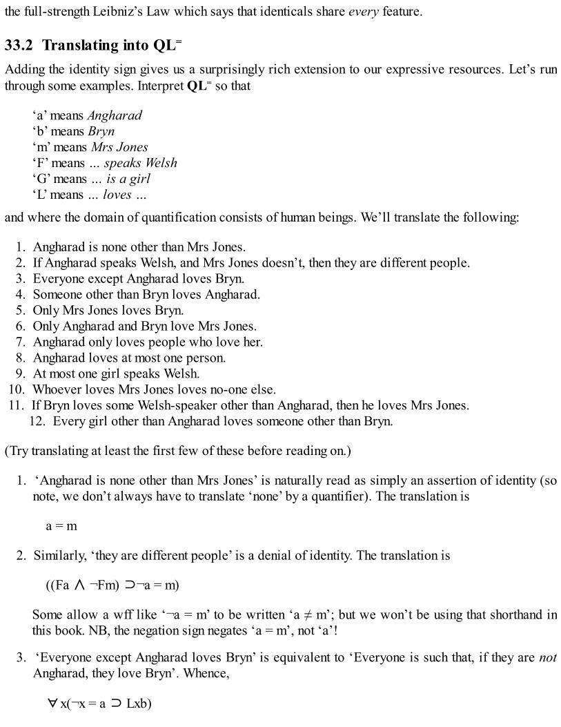
the full-strength Leibniz’s Law which says that identicals share every feature.

33.2 Translating into QL=

Adding the identity sign gives us a surprisingly rich extension to our expressive resources. Let’s runthrough some examples. Interpret QL= so that

‘a’ means Angharad‘b’ means Bryn‘m’ means Mrs Jones‘F’ means … speaks Welsh‘G’ means … is a girl‘L’ means … loves …

and where the domain of quantification consists of human beings. We’ll translate the following:

1. Angharad is none other than Mrs Jones.2. If Angharad speaks Welsh, and Mrs Jones doesn’t, then they are different people.3. Everyone except Angharad loves Bryn.4. Someone other than Bryn loves Angharad.5. Only Mrs Jones loves Bryn.6. Only Angharad and Bryn love Mrs Jones.7. Angharad only loves people who love her.8. Angharad loves at most one person.9. At most one girl speaks Welsh.

10. Whoever loves Mrs Jones loves no-one else.11. If Bryn loves some Welsh-speaker other than Angharad, then he loves Mrs Jones.

12. Every girl other than Angharad loves someone other than Bryn.

(Try translating at least the first few of these before reading on.)

1. ‘Angharad is none other than Mrs Jones’ is naturally read as simply an assertion of identity (sonote, we don’t always have to translate ‘none’ by a quantifier). The translation is

a = m

2. Similarly, ‘they are different people’ is a denial of identity. The translation is

((Fa ∧ ¬Fm) ⊃¬a = m)

Some allow a wff like ‘¬a = m’ to be written ‘a ≠ m’; but we won’t be using that shorthand inthis book. NB, the negation sign negates ‘a = m’, not ‘a’!

3. ‘Everyone except Angharad loves Bryn’ is equivalent to ‘Everyone is such that, if they are notAngharad, they love Bryn’. Whence,

∀x(¬x = a ⊃ Lxb)

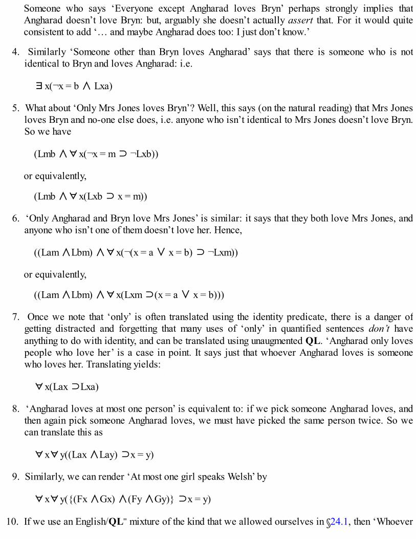
Someone who says ‘Everyone except Angharad loves Bryn’ perhaps strongly implies thatAngharad doesn’t love Bryn: but, arguably she doesn’t actually assert that. For it would quiteconsistent to add ‘… and maybe Angharad does too: I just don’t know.’

4. Similarly ‘Someone other than Bryn loves Angharad’ says that there is someone who is notidentical to Bryn and loves Angharad: i.e.

∃x(¬x = b ∧ Lxa)

5. What about ‘Only Mrs Jones loves Bryn’? Well, this says (on the natural reading) that Mrs Jonesloves Bryn and no-one else does, i.e. anyone who isn’t identical to Mrs Jones doesn’t love Bryn.So we have

(Lmb ∧∀x(¬x = m ⊃ ¬Lxb))

or equivalently,

(Lmb ∧∀x(Lxb ⊃ x = m))

6. ‘Only Angharad and Bryn love Mrs Jones’ is similar: it says that they both love Mrs Jones, andanyone who isn’t one of them doesn’t love her. Hence,

((Lam ∧Lbm) ∧∀x(¬(x = a ∨ x = b) ⊃ ¬Lxm))

or equivalently,

((Lam ∧Lbm) ∧∀x(Lxm ⊃(x = a ∨ x = b)))

7. Once we note that ‘only’ is often translated using the identity predicate, there is a danger ofgetting distracted and forgetting that many uses of ‘only’ in quantified sentences don’t haveanything to do with identity, and can be translated using unaugmented QL. ‘Angharad only lovespeople who love her’ is a case in point. It says just that whoever Angharad loves is someonewho loves her. Translating yields:

∀x(Lax ⊃Lxa)

8. ‘Angharad loves at most one person’ is equivalent to: if we pick someone Angharad loves, andthen again pick someone Angharad loves, we must have picked the same person twice. So wecan translate this as

∀x∀y((Lax ∧Lay) ⊃x = y)

9. Similarly, we can render ‘At most one girl speaks Welsh’ by

∀x∀y({(Fx ∧Gx) ∧(Fy ∧Gy)} ⊃x = y)

10. If we use an English/QL= mixture of the kind that we allowed ourselves in 24.1, then ‘Whoever

loves Mrs Jones loves no-one else’ is semi-translated by

∀x(Lxm ⊃x loves no-one other than Mrs Jones)

But ‘x loves no-one other than Mrs Jones’ can be translated as

∀y(¬y = m ⊃¬Lxy)

or equivalently,

∀y(Lxy ⊃y = m)

And plugging that in the half-completed translation, we finally get:

∀x(Lxm ⊃∀y(Lxy ⊃y = m))

As always, we could alternatively translate the ‘no-one’ quantification using the existentialquantifier:

∀x(Lxm ⊃¬∃y(Lxy ∧¬y = m))

11. The antecedent ‘Bryn loves some Welsh-speaker other than Angharad’ is translated by

∃x((Lbx ∧Fx) ∧¬x = a)

So the whole conditional translates as follows:

(∃x((Lbx ∧Fx) ∧¬x = a) ⊃Lbm)

12. Finally, we’ll again take ‘Every girl other than Angharad loves someone other than Bryn’ instages. As a half-way house we have this:

∀x((Gx ∧¬x = a) ⊃x loves someone other than Bryn)

Then ‘x loves someone other than Bryn’ translates as

∃y(Lxy ∧¬y = b)

So putting those together we get

∀x((Gx ∧¬x = a) ⊃∃y(Lxy ∧¬y = b))

33.3 Numerical quantifiersWe have just seen how to translate ‘there is at most one F’:

(1) ∀x∀y((Fx ∧Fy) ⊃x = y)

We know from before how to translate ‘there is at least one F’:

(2) ∃xFx

Putting these together, then, we can translate ‘there is exactly one F’ (i.e. there is at least one and atmost one F) by the conjunction:

(3) (∃xFx ∧∀x∀y((Fx ∧Fy) ⊃x = y))

Here’s an alternative, simpler, translation that will do as well:

(4) ∃x(Fx ∧∀y(Fy ⊃y = x))

(Convince yourself that those two indeed come to the same!) And here’s an even simpler version:

(5) ∃x∀y(Fy≡y = x)

We can formally show that (4) and (5) are q-equivalent, i.e. q-entail each other (see 35.1). But thisresult too should look intuitively right. For suppose x is the one and only F. Then take anything y youlike, if it is identical to x it is F (which gives you one direction of the biconditional); and if y is F itmust be none other than x again (which gives you the other direction of the biconditional).Incidentally, you will find that (4) – or equivalently (5) – is quite often abbreviated as

(6) ∃!xFx

But we won’t adopt that notation here.Now consider the following wffs,

(7) ∃x∃y((Fx ∧Fy) ∧¬x = y)

(8) ∀x∀y∀z(((Fx ∧Fy) ∧Fz) ⊃((x = y ∨y = z) ∨z = x))

The first says that there is an F and also another, distinct F. In other words, (7) says that there are atleast two Fs.

Note – by the way of a quick aside – that we can, if we want, similarly translate a proposition like‘Some philosophers are logicians’ into QL= and retain the indication that there is more than onelogical philosopher, by writing e.g.

(7*) ∃x∃y(((Gx ∧Hx) ∧(Gy ∧Hy)) ∧¬x = y)

(8), to continue, says that if we try to pick three things which are all F, then at least two of the Fswill be identical – i.e., there are at most two Fs. The conjunction of (7) with (8) will therefore saythat there are at least two Fs and at most two Fs, or in other words that there are exactly two Fs. Orwe could equally well, and more neatly, translate that by

(9) ∃x∃y({(Fx ∧Fy) ∧¬x = y} ∧∀z{Fz ⊃(z = x ∨z = y)})

which says that there is an F and another distinct F and any F you choose has to be one of those.Similarly

(10) ∃x∃y∃z({((Fx ∧Fy) ∧Fz) ∧((¬x = y ∧¬y = z) ∧¬z = x)} ∧∀w{Fw ⊃ ((w = x∨w = y) ∨w = z)})

says that you can find three Fs, all different, and any F you choose is one of them – in other wordsthere are exactly three Fs.

We can obviously keep going in a similar vein, expressing numerical quantifications (‘there are atleast n Fs’, ‘there are at most n Fs’, ‘there are exactly n Fs’) using just the familiar quantifiers, theconnectives, and identity.

But the link between logic and elementary arithmetic is closer than a mere point about QL=’scapacity to express numerical quantifiers. For suppose we abbreviate the forms (4), (9) and (10)respectively by ‘∃1vFv’, ‘∃2vFv’, ‘∃3vFv’. Then consider the long wff we can then abbreviate as

(11) ({(∃2vFv ∧∃1vGv) ∧¬∃x(Fx ∧Gx)} ⊃∃3v(Fv ∨Gv))

What does this say? That if there are two F and one G (and nothing is F and G), then we have threethings that are F-or-G. For example, if there are two things in my left hand, and one thing in my right,then there are three things in my hands altogether. Or, as we learnt to say in nursery school, two andone makes three.

So here we find that a bit of simple applied arithmetic is also expressible in QL=. But more thanthat, not only is this truth expressible in logical terms, but it is in fact a q-logical truth: it can beshown, with a bit of effort, to be true on all q-valuations. Which raises an intriguing, deep anddifficult question: just how much arithmetic is, so to speak, just logic in disguise?

33.4 SummaryWe add to QL the identity sign – governed by the syntactic rule that a term followed by ‘=’followed by a term is an atomic wff – to get QL=.The identity sign is governed by the semantic rule that an atomic wff of the form ‘t1 = t2’ is trueon the valuation q iff the terms t1 and t2 have the same reference according to q.QL= has the resources to express more complex quantifiers like ‘Everyone other than Angharad…’, ‘Exactly three people …’, ‘No one else …’ etc.

Exercises 33A More Welsh affairs! Using the same translation manual as 33.2, translate the following into QL=:

1. Angharad and Mrs Jones are one and the same.2. At least one Welsh speaker loves Bryn.3. Either Angharad or Bryn is Mrs Jones.4. Someone other than Bryn loves Angharad.

5. Mrs Jones loves everyone but Angharad.6. Some girls only love Bryn.7. Some girls only love people who love them.8. Only if she loves Bryn is Angharad loved by him.9. Exactly one girl who loves Bryn speaks Welsh.

10. If Angharad isn’t Mrs Jones, then at least two people love Bryn.

B Take the domain of quantification to be the (positive whole) numbers, and let ‘m’ denote thenumber zero, ‘n’ denote the number one, let ‘Mxy’ mean that x immediately follows y in thenumber series (equivalently, x is an immediate successor of y), and ‘Rxyz’ mean that x equals yplus z. Then translate the following from QL= into natural English:

1. ∀x∀y∀z((Mxz ∧Myz) ⊃x = y)2. ∀y∃xMxy3. ¬∃zMmz4. ∀x∀y∀z((Mxy ∧y = z) ⊃Mxz)5. ∀x∀y(Rxym ⊃x = y)6. ∀x∀y(Rxyn ⊃Mxy)7. ∀x∀y∀z(Rxyz≡Rxzy)8. ∃x(Rxxx ∧∀y(Ryyy ⊃y = x))9. ∀x∀y∃z(Rzxy ∧∀v0(Rv0xy ⊃v0 = z))

10. ∀z∃x((Mxz ∧∀y(Myz ⊃y = x)) ∧Rznx)11. ∃x∃y({[((Mxm ∨Mxn) ∧(Mym ∨Myn))] ∧¬x = y} ∧∀z{(Mzm ∨Mzn) ⊃(z = x ∨z

= y)})

34

Descriptions and existence

In this chapter, we extend our discussion of the expressive resources of QL= by considering how‘definite descriptions’ – i.e. expressions of the kind the F – can be translated using Russell’s Theoryof Descriptions. We will also see how various statements about existence can be translated.

34.1 Definite descriptionsConsider the expressions ‘the man in the corner drinking a martini’, ‘the oldest woman in the world’,‘the Queen of England’, ‘the smallest prime number’, ‘the present King of France’, ‘the largest primenumber’. Such expressions – more generally, expressions of the type ‘the (one and only) F’ – arestandardly called definite descriptions. A definite description is a designator, or more accurately itaims to designate a particular thing. As the last two cases remind us, definite descriptions may in factfail to pick out any entity: there may be nothing which is F, and so nothing which is the F.

Imagine we are at a party. I tell you that a number of professors from different disciplines are here,and say ‘The philosopher is over there, talking to George’. Then it certainly seems that you can inferthat there is (at least) one philosopher present.

Generalizing, if a claim of the form ‘The F is G’ is true, then so is the corresponding claim of theform ‘There is at least one F’ (ignoring for the moment some rogue cases, where G is filled by e.g.‘non-existent’ or ‘fictitious’).

Suppose we want to reflect this sort of logical entailment inside QL or QL=. How can we do that?Take ‘F’ to mean … is a philosopher and ‘G’ to mean … is talking to George; and let the domain

be, say, people present at the party. And imagine first that we render the designator ‘the philosopher’by a simple constant ‘n’. Then the valid inference ‘The philosopher present is talking to George; sothere is at least one philosopher present’ would get translated by something like ‘Gn ∴ ∃xFx’,which is of course not q-valid. The translation of ‘the philosopher’ by the simple constant ‘n’ misseslogically relevant structure: it ignores the key fact that the definite description embeds the predicate‘philosopher’.

Moral: if we want to capture the logical behaviour of definite descriptions, we need some way oftranslating them into our formalized language that similarly embeds the relevant predicate.

How shall we proceed? Well, remember that we can express the proposition that there is one andonly one philosopher at the party as follows (compare 33.3, (4)):

(1) ∃x(Fx ∧∀y(Fy ⊃ y = x))

Suppose we want to add that this one and only philosopher is talking to George. Then we can just addanother conjunct inside the scope of the quantifier:

(2) ∃x((Fx ∧∀y(Fy ⊃ y = x)) ∧Gx)

But now note, the claim (2) – there is one and only one philosopher (here at the party), and he istalking to George – seems to come to more or less the same as this: the philosopher (here at theparty) is talking to George. For if there is one and only one philosopher present, there is indeedsomeone to be the philosopher; and (2) says that that person is talking to George. Note too that (2)pretty trivially q-entails

(3) ∃xFx

So the rendition (2) does enable us to reflect in QL= the valid inference from ‘The philosopher (hereat the party) is talking to George’ to ‘There is a philosopher (here at the party)’.

Instead of (1), we could equally well use

(1′) ∃x∀y(Fy≡y = x)

to render the proposition that there is one and only one philosopher (compare 33.3, (5)). And hence,instead of (2), we could equally well use the snappier

(2′) ∃x∀y((Fy≡y = x) ∧Gx) or∃x(∀y(Fy≡y = x) ∧Gx)

to render the proposition that the philosopher is talking to George.And a third equivalent way of saying the same is the more long-winded

(2″) ({∃xFx ∧∀x∀y((Fx ∧Fy) ⊃ x = y)} ∧∀x(Fx ⊃ Gx))

i.e. ‘There is at least one philosopher and there is at most one philosopher and whoever is aphilosopher is talking to George’. In the next chapter we will develop the resources to show that (2),(2′) and (2″) are indeed q-equivalent, i.e. they q-entail each other: but for the moment let’s take thisintuitively correct claim on trust.

Generalizing – and fixing on translations like (2) or (2′) rather than (2″) for reasons of brevity –these remarks suggest the following thesis:

We can render a sentence of the kind ‘The F is G’ into QL= by corresponding wffs of the form

(R) ∃v((Fv ∧∀w(Fw ⊃ w = v)) ∧Gv)(R′) ∃v∀w((Fw≡w = v) ∧Gv)

(In stating the thesis this way, the metalinguistic ‘F’ and ‘G’ do double duty in a now familiar way,first holding the place for English expressions, and then holding the place for the respectivetranslations of these expressions into QL=: but the intended idea should be clear enough.)

The claim that The F is G can be rendered into QL= by (R) or (R′) is due to Bertrand Russell. It ispart of his famed Theory of Descriptions. But this Theory says quite a lot more. For Russell alsoclaims:

Translating The F is G by (R) is not merely the best available option, given the limited resourcesof QL=, but is fully accurate, in the sense of getting it exactly right about the conditions underwhich The F is G is true and the conditions under which it is false.

Moreover, the QL= translation reflects the true underlying logical form of sentences involvingdefinite descriptions. Descriptions really are, in some sense, a kind of quantifier in disguise.

Let’s briefly take these additional Russellian claims in turn.Plausibly, as we said, if (R) is true, then The F is G is true. But do the two match on falsehood?Suppose that there is no F. Then anything of the form ‘∃v(Fv ∧ …)’ will be false. Hence the QL=

rendition of The F is G comes out plain false when there is no F. Would we want to say the same,however, about The F is G? Russell himself uses the example ‘The present King of France is bald’. Isthis straightforwardly false? Maybe this sort of claim is better described as not even making thestarting line for consideration for being true or false, since the definite description fails to pick out areferent. In other words, we might want to say that the claim is neither true nor false.

Compare ‘Mr Brixintingle is bald’, where the apparent proper name ‘Mr Brixintingle’ is just afake, invented to look vaguely name-like, but in fact attached to no-one. That sentence fails to makeany determinate claim, and so plausibly lacks a truth-value. In other words, non-referring namesarguably create truth-value gaps. The anti-Russellian suggestion is that non-referring descriptions doso too. And if that is right, ‘The present King of France is bald’ – neither true nor false – is notequivalent to ‘There is one and only one King of France, and he is bald’, or to a rendition like (2) –which is straightforwardly false.

Now, it is agreed on all sides that a claim of the form The F is G can fail to be true in more thanone way. It can fail (a) because there isn’t an F; it can fail (b) because there are too many Fs (so weshouldn’t talk of the F); it can fail (c) when there is a unique F but it isn’t G. The Russellian willclaim that his rendition (R) captures this very nicely: The F is G can be false in three different ways,depending on which of the three conjuncts in the analysis (R) isn’t satisfied. The anti-Russelliandisagrees, and will instead say that only in case (c) is the claim actually false; in cases (a) and (b)The F is G is neither true nor false.

But what does this disagreement really come to? How do we decide such issues?It is very unclear what to say, and the principles that should guide debate here are intensely

disputed. We certainly can’t pursue these matters any further in this book. We just have to note thatthere is a minefield hereabouts!

There is another minefield around claims to do with ‘logical form’. Suppose that (R) does get itright about when The F is G is true and when it is false. It remains quite unclear what cash-value wecan give to the thesis that (R) somehow reveals the true semantic structure of vernacular claimsinvolving definite descriptions. And it is again quite obscure how we are to evaluate such claims. InChapter 36, we’ll say just a little more that is germane to these vexed issues, but without any hope ofresolving them.

So for the moment let’s set aside both of Russell’s more ambitious claims, and stick to basics. Thismuch, at any rate, is uncontroversial: given the limited resources of QL=, wffs of the Russellian form(R), (R′), or their equivalents, are the best we can do in rendering sentences involving definitedescriptions. We’ll therefore use the schemas (R) or (R′) henceforth, whenever we need to translatedescriptions.

34.2 Descriptions and scopeOne arguable resemblance between definite descriptions and quantifiers (not in itself enough towarrant treating the first as a disguised form of the second, but a suggestive resemblance none the

less) is that descriptions exhibit what plausibly can be construed as scope phenomena (compare 21.3). For example, just as ordinary-language quantifiers mixed with negation can produce scopeambiguity, so ordinary-language definite descriptions mixed with negation can produce ambiguity.

Suppose we are discussing famous baldies. You challenge me to name ten. I reel off a listbeginning

Yul Brynner is bald,Bruce Willis is bald,the actor who plays ‘Captain Picard’ in Star Trek is bald,the King of France is bald,

and you interrupt, saying

(A) No! That last one’s not right. The King of France isn’t bald – he doesn’t even exist!

Your protest is surely correct, and the way you have phrased it seems natural enough. But nowcompare a second occasion. This time we are discussing people who aren’t bald. So this time I reeloff a list of famous non-baldies:

The Queen of England isn’t bald,George W. Bush isn’t bald,Bill Clinton isn’t bald,

(B) the King of France isn’t bald,

and again you interrupt, this time saying

No! That’s not right. You can’t say that – he doesn’t even exist!

Again, you are surely right. But how can it be that my assertion (B) is flawed, when you, using exactlythe same words in (A), were saying something correct?

We will have to discern an ambiguity. ‘The King of France isn’t bald’ can be used to express twodifferent claims, one true, the other false. And Russell’s Theory of Descriptions gives us a very neatdiagnosis of the apparent ambiguity here; it treats it as a straightforward scope ambiguity. On onereading, the negation has wide scope, governing the whole sentence, and the resulting message can berendered

(1) ¬∃x((Fx ∧∀y(Fy ⊃ y = x)) ∧Gx)

This captures the truth that you asserted in (A). On the other reading, the negation has narrow scope,governing just the predicate ‘bald’, and the resulting message can be rendered

(2) ∃x((Fx ∧∀y(Fy ⊃ y = x)) ∧¬Gx)

And this is the falsehood which I apparently asserted in (B).Here’s another case of scope ambiguity, a modal case worth mentioning even though it takes us

beyond the resources of pure QL=. Consider:

(3) The President might have been a woman.

This again has two readings. Are we saying there’s a possible scenario in which a different politicalhistory leads to a President in that scenario who is a woman? Or are we saying of the actualPresident, that he (that very person) might have been a woman – contemplating some kind of sexchange, perhaps? If we imagine adding a modal operator ‘ ’ to be read as ‘It might have been thecase that’, then the Russellian will represent this ambiguity as between giving ‘ ’ wide or narrowscope, along the following lines:

(4) ∃x((Fx ∧∀y(Fy ⊃ y = x)) ∧Gx)

or

(5) ∃x((Fx ∧∀y(Fy ⊃ y = x)) ∧ Gx)

34.3 More translationsA few more quick examples. We’ll use the translation manual

‘a’ means Angharad‘b’ means Bryn‘m’ means Mrs Jones‘F’ means … speaks Welsh‘G’ means … is a girl‘L’ means … loves …‘M’ means … is taller than …

and where the domain of quantification again consists of human beings, and translate the followinginto QL=:

1. The Welsh speaker who loves Mrs Jones is taller than her.2. Bryn loves the girl who loves him.3. Bryn only loves the girl who loves him.4. The tallest girl speaks Welsh.5. The girl who loves Bryn loves the Welsh speaker who loves Angharad.

1. The first involves the definite description ‘The Welsh speaker who loves Mrs Jones’, and ‘x is aWelsh speaker who loves Mrs Jones’ is translated by ‘{Fx ∧Lxj}’. So following the Russellianschema (R), the complete translation will run

∃x(({Fx ∧Lxj} ∧∀y({Fy ∧Lyj} ⊃ y = x)) ∧Mxj)

If we’d used schema (R′), we’d get the brisker

∃x∀y(({Fy ∧Lyj}≡⊃ y = x) ∧Mxj)

2. This is similar: the definite description this time is ‘The girl who loves Bryn’, and ‘x is a girl who

loves Bryn’ is translated by ‘{Gx ∧Lxb}’. Using (R) again we arrive at

∃x(({Gx ∧Lxb} ∧∀y({Gy ∧Lyb} ⊃ y = x)) ∧Lbx)

We’ll leave the (R′)-style version to be done as an exercise.

3. To translate this, we need to add that for anyone other than this girl, x, Bryn does not love x; orequivalently, anyone he does love is none other than x again. Whence

∃x[(({Gx ∧Lxb} ∧∀y({Gy ∧Lyb} ⊃ y = x)) ∧Lbx) ∧∀z(Lbz ⊃ z = x)]

4. The tallest girl is the girl such that she is taller than all other girls. Now, ‘y is a girl who is tallerthan all other girls’ can be rendered ‘{Gy ∧∀z((Gz ∧ ¬z = y) ⊃Mzy)}. Plugging that into thesimpler (R′) schema, we get

∃x∀y(({Gy ∧∀z((Gz ∧¬z = y) ⊃Mzy)} ≡y = x) ∧Fx)

This time, we’ll leave the longer (R)-style version as an exercise.

5. Our last example involves two descriptions. Abbreviate ‘loves the Welsh speaker who lovesAngharad’ by ‘C’. And to reduce clutter, let’s again use schema (R′) straight off. Then we have, ashalf-way translations,

The girl who loves Bryn is C

∃x∀y(({Gy ∧Lyb}≡y = x) ∧Cx)

And (using different variables, so we don’t get into a tangle),

Cx ∃z∀w(({Fw ∧Lwa}≡w = z) ∧Lxz)

So, if we plug the one into the other, we get

∃x∀y(({Gy ∧Lyb}≡y = x) ∧∃z∀w(({Fw ∧Lwa}≡w = z) ∧Lxz))

The last translation does the trick! However, the messiness of this QL= rendition compared to therelative simplicity of the original English might very arguably begin to cast some doubt on theRussellian thesis that the Theory of Descriptions captures the true underlying ‘logical form’ of thevernacular claim.

34.4 Existence statementsWe’ll consider three types of existential statement:

examples like ‘Tame tigers exists’ and ‘Unicorns don’t exist’, i.e. statements of the kind ‘Fsdo/don’t exist’, with F filled by some more or less complex specification of a kind of thing;examples like ‘The Queen of England exists’ and ‘The King of France doesn’t exist’, i.e.statements of the kind ‘The F does/doesn’t exist’, with ‘The F’ a definite description;examples like ‘Gwyneth Paltrow exists’ (she’s a living breathing actress) and ‘Lois Lane doesn’texist’ (not really, she’s just a fictional character).

How do we render such claims into QL=?The first case is easy. ‘Tame tigers exist’ is equivalent to ‘There are some tame tigers’, so can be

rendered as

(1) ∃x(Fx ∧ Gx)

with the obvious interpretation of the predicates. Or if you want explicitly to capture the thought thatthere is more than one, as signalled by the English plural, then you can write:

(2) ∃x∃y({(Fx ∧ Gx) ∧(Fy ∧ Gy)} ∧¬x = y)

Likewise, ‘Unicorns don’t exist’, which is equivalent to ‘It is not the case that there are someunicorns’, can be rendered by

(3) ¬∃xHx

What about ‘The Queen of England exists’ and ‘The present King of France doesn’t exist’?The simplest suggestion is this. To say that the Queen of England exists is just to say that there is

one and only one (present) Queen of England. Rendering that into QL= (using ‘F’ for … is a Queen ofEngland), we’ll get

(4) ∃x(Fx ∧∀y(Fy ⊃ y = x))

And if we negate the whole thing –

(5) ¬∃x(Fx ∧∀y(Fy ⊃ y = x))

– we get something which, changing the translation manual, will render the claim that the present Kingof France does not exist.

Unsurprisingly, then, existence claims involving predicative expressions and definite descriptionsget rendered into QL= using the existential quantifier. But what about the third type of existence claim,the type involving names?

Take that interpretation of QL= which reads ‘m’ as a name of Gwyneth Paltrow. Can’t we simplyexpress the thought that Gwyneth exists, i.e. that there is indeed someone who is Gwyneth, asfollows? –

(6) ∃x x = m

At first sight, that looks satisfactory; but on reflection, there’s a problem. For note, (6) is a q-logicaltruth!

Why so? Well, consider any q-valuation q of the vocabulary in ‘∃x x = m’. By definition, q has toassign an object m to be the reference of ‘m’. And so q will always have an extension q+ which alsoassigns m to the variable ‘x’; hence q will always have an extension q+ which makes ‘x = m’ true. So,by definition, ‘∃x x = m’ is true on any q-valuation of its vocabulary. But if ‘∃x x = m’ is a q-logical

truth, then (we might surmise) it can’t really be a ideal rendition of ‘Gwyneth Paltrow exists’ (whichof course isn’t a logical truth).

To press the point further, consider the claim ‘Lois Lane doesn’t exist’. That’s another truth. But wecan’t render it into QL= by writing something like

(7) ¬∃x x = n

since (7) is false on all q-valuations of its vocabulary.Of course, these results about the status of (6) and (7) directly reflect the stipulation that q-

valuations assign a reference to any constant that is in play. By contrast, ordinary language has ‘emptynames’, names which fail to pick out an object, yet which have a role in the language and don’tproduce mere nonsense. In the Fregean terminology of 31.1, it seems that ordinary names can havesense even if that lack reference. That is why it is contentful to be told that Lois Lane or Santa Clausdon’t exist, but that there is such a person as Gwyneth.

There are two reactions we can have to all this.

One line is to proceed to extend QL and QL= to allow meaningful but non-denoting names. Thisyields a so-called free logic, i.e. a logic free of certain existence assumptions.The other line is to cling to the simplicity of QL/QL= (on the grounds that there is, after all, asense in which non-denoting names are linguistically defective when used in serious, fact-statingdiscourse, and we are in the business of constructing a logically ideal language).

Now, adopting a free logic does involve significant revisions and complications; so, rightly orwrongly, the second reaction is the standard one. But if we do stick to the standard semantic storyabout QL/QL=, then we must be aware of the implications of the built-in assumption that everyconstant we actually use has an object as its q-value, i.e. has a reference.

To summarize: in our languages QL and QL=, we require any constant we use to have a referencein the domain of discourse. The logical truths of those languages are then truths that are guaranteedonce that assumption of reference is in place. In particular, a wff like ‘∃x x = n’ always comes outtrue on a q-valuation. In this respect, there is arguably significant slippage between the semanticnature of some QL= wffs and the apparently corresponding ordinary language sentences. And becauseof that, there will be some q-valid (and hence valid) QL= arguments whose most tempting Englishrenditions are not valid. (Compare the argument of 28.4.)

A quick final remark. Apprentice philosophers often come across the slogan ‘Existence isn’t apredicate’. If this is read as saying that a language can’t have a predicative expression (i.e. anexpression with one slot waiting to be filled up by a designator) which applies to all the thingsassumed to exist in its domain of quantification, then the slogan misleads. In QL=, ‘∃x x = …’ woulddo the job perfectly: it is true of everything in the domain. The same expression works just as well insome free logics too. But if the philosophical slogan is intended to bring out the close relationbetween vernacular existence talk and the use of something fundamentally different from an ordinarypredicate, namely the operation of existential quantification, then the slogan is apt.

34.5 SummarySentences of the form The F is G are best rendered into QL= by a corresponding wff of the form

‘∃v((Fv ∧∀w(Fw ⊃ w = v)) ∧Gv)’, or equivalently by ‘∃v∀w((Fw≡w = v) ∧Gv)’.This uncontentious claim, part of Russell’s Theory of Descriptions, should be distinguished fromRussell’s much more contentious claims that this rendition gets the truth-conditions of The F is Gexactly right, and moreover in some sense reveals the true logical form of vernacular statementsinvolving descriptions.However, Russell’s analysis plausibly diagnoses certain apparent ambiguities involvingdescriptions as being scope ambiguities.Existential claims are naturally rendered using the existential quantifier (though there areproblems about cases involving proper names, given the assumption built into the semantics ofQL and QL= that names always have referents).

Exercises 34Yet more Welsh affairs! Using the same translation manual as 34.3, translate the following into QL=:

1. The Welsh speaker loves Mrs Jones.2. The girl who loves Angharad does not loves Bryn.3. Angharad loves the girl who loves Bryn.4. The Welsh speaker who loves Mrs Jones is either Angharad or Bryn.5. Someone other than the girl who loves Bryn is taller than Angharad.6. The one who loves Angharad is the one she loves.7. Only if she loves him does Bryn love the girl who speaks Welsh.8. The girl other than the girl who loves Bryn is Angharad.9. The shortest Welsh speaker loves Bryn.

10. The shortest Welsh speaker loves the tallest Welsh speaker.

35

Trees for identity

We now expand our treatment of quantifier trees to cover arguments involving identity, expressed inQL=. We first introduce and motivate two rules dealing with wffs involving identity. We exploresome introductory examples and also show that these rules can be used to demonstrate that the basiclaws of identity are q-logical truths. Then we consider some examples involving definite descriptionsand numerical quantifiers.

35.1 Leibniz’s Law againTake the argument: ‘Bertie is clever. Bertie is none other than Russell. So Russell is clever.’ That’svalid. Translating, we have

A Fm, m = n ∴ Fn

Starting a signed tree in the standard way, we suppose that there is a valuation q such that

(1) Fm ⇒q T(2) m = n ⇒q T(3) ¬Fn ⇒q T

How are we to proceed now? Consider again Leibniz’s Law, in the form we met in 32.5:

(LL′)If ‘a’ and ‘b’ are functioning as co-referential designators in the claims C(…a…a…) andC(…b…b…), and also the context C expresses the same property in each case, then theseclaims say the same about the same thing, and so must have the same truth-value.

We noted that, in English, different occurrences of the same predicate need not attribute the sameproperty (remember the behaviour of ‘… is so-called because of his size’). But in our tidy artificiallanguage QL= we just don’t have that troublesome kind of predicate. And our official semanticsindeed implies

(A) If ‘m’ and ‘n’ are co-referential designators according to q, then the claims ‘Fm’ and ‘Fn’must have the same truth-value on q.

Further, it is immediate that

The atomic wff ‘m = n’ is true on the valuation q just if ‘m’ and ‘n’ are assigned the same

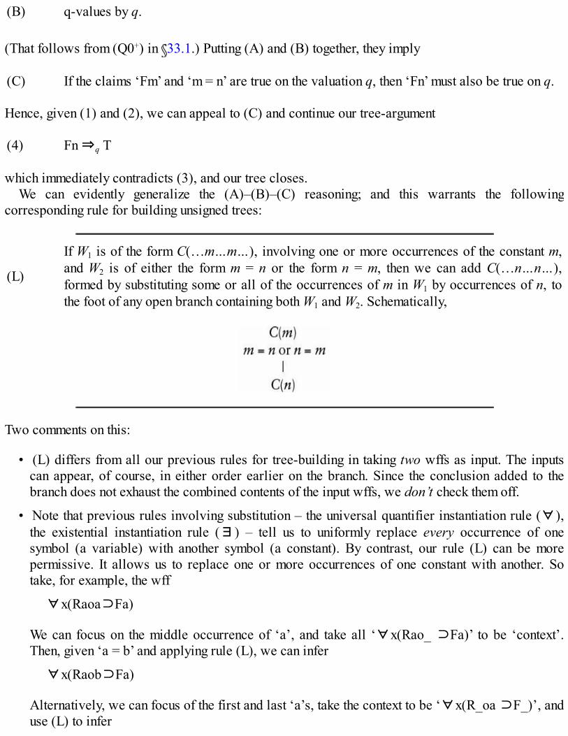
(B) q-values by q.

(That follows from (Q0+) in 33.1.) Putting (A) and (B) together, they imply

(C) If the claims ‘Fm’ and ‘m = n’ are true on the valuation q, then ‘Fn’ must also be true on q.

Hence, given (1) and (2), we can appeal to (C) and continue our tree-argument

(4) Fn ⇒q T

which immediately contradicts (3), and our tree closes.We can evidently generalize the (A)–(B)–(C) reasoning; and this warrants the following

corresponding rule for building unsigned trees:

(L)

If W1 is of the form C(…m…m…), involving one or more occurrences of the constant m,and W2 is of either the form m = n or the form n = m, then we can add C(…n…n…),formed by substituting some or all of the occurrences of m in W1 by occurrences of n, tothe foot of any open branch containing both W1 and W2. Schematically,

Two comments on this:

• (L) differs from all our previous rules for tree-building in taking two wffs as input. The inputscan appear, of course, in either order earlier on the branch. Since the conclusion added to thebranch does not exhaust the combined contents of the input wffs, we don’t check them off.

• Note that previous rules involving substitution – the universal quantifier instantiation rule (∀),the existential instantiation rule (∃) – tell us to uniformly replace every occurrence of onesymbol (a variable) with another symbol (a constant). By contrast, our rule (L) can be morepermissive. It allows us to replace one or more occurrences of one constant with another. Sotake, for example, the wff

∀x(Raoa⊃Fa)

We can focus on the middle occurrence of ‘a’, and take all ‘∀x(Rao_ ⊃Fa)’ to be ‘context’.Then, given ‘a = b’ and applying rule (L), we can infer

∀x(Raob⊃Fa)

Alternatively, we can focus of the first and last ‘a’s, take the context to be ‘∀x(R_oa ⊃F_)’, anduse (L) to infer

∀x(Rboa⊃Fb).

Or, of course, we can infer the result of simultaneously replacing all three occurrences of ‘a’.Each inference is plain valid.

So now let’s take some simple examples of our rule (L) in operation.First, consider the argument

B Either Alice or Mrs Brown is the winner. Alice isn’t the winner. So Alice isn’t MrsBrown.

It is trivial to render this into QL=, and the resulting tree is equally straightforward:

Here, the only step worth remarking on is (6), where we have used (L) to derive ‘Fa’ from (5) ‘Fb’and (4) ‘a = b’. The tree closes, hence the intuitively valid argument (B) is, as we’d expect, q-valid.

For another example, consider the following:

C Only Russell is a great philosopher. Bertrand is a great philosopher who smokes. HenceRussell smokes.

Put ‘F’ for great philosopher, ‘G’ for smokes, etc., and we can render this:

(Fm ∧∀x(Fx⊃x = m)), (Fn ∧Gn) ∴ Gm

A tree can then be constructed as follows:

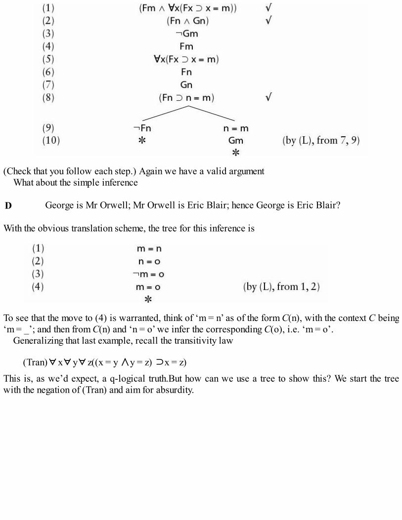
(Check that you follow each step.) Again we have a valid argumentWhat about the simple inference

D George is Mr Orwell; Mr Orwell is Eric Blair; hence George is Eric Blair?

With the obvious translation scheme, the tree for this inference is

To see that the move to (4) is warranted, think of ‘m = n’ as of the form C(n), with the context C being‘m = _’; and then from C(n) and ‘n = o’ we infer the corresponding C(o), i.e. ‘m = o’.

Generalizing that last example, recall the transitivity law

(Tran)∀x∀y∀z((x = y ∧y = z) ⊃x = z)

This is, as we’d expect, a q-logical truth.But how can we use a tree to show this? We start the treewith the negation of (Tran) and aim for absurdity.

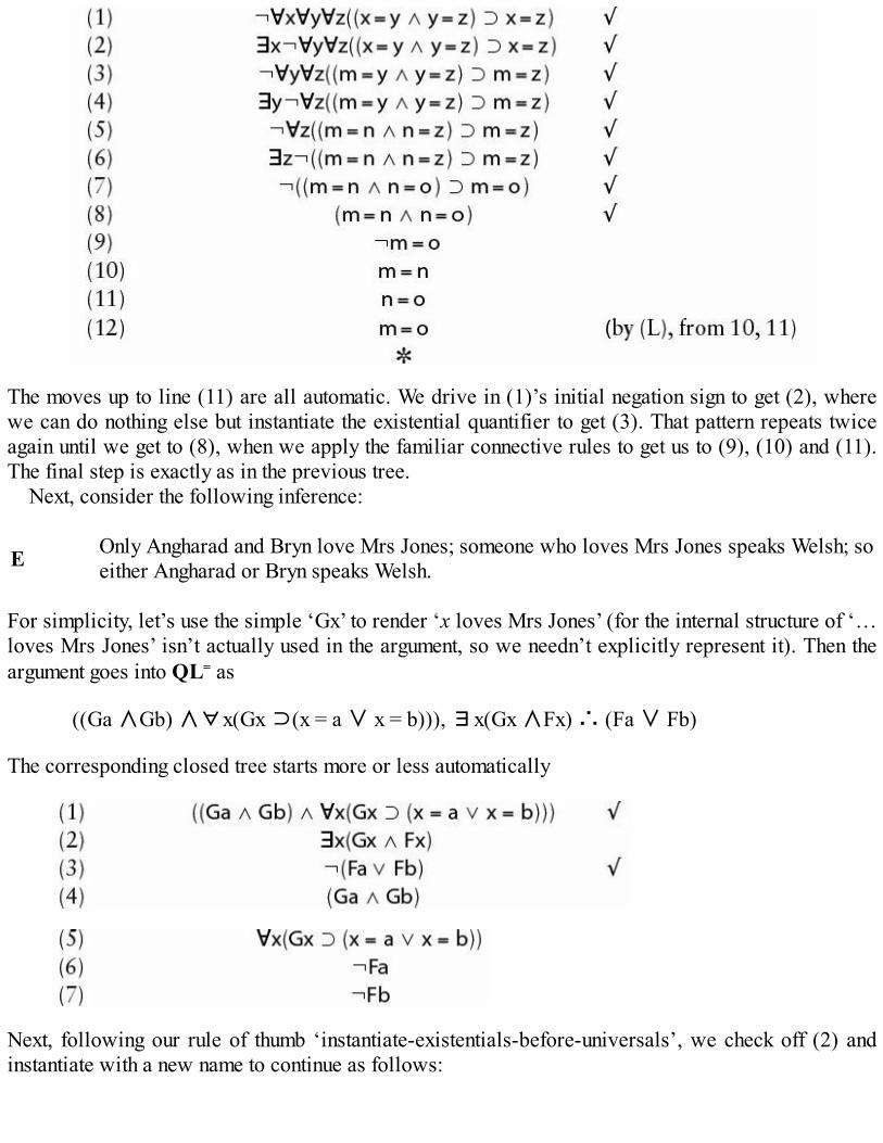
The moves up to line (11) are all automatic. We drive in (1)’s initial negation sign to get (2), wherewe can do nothing else but instantiate the existential quantifier to get (3). That pattern repeats twiceagain until we get to (8), when we apply the familiar connective rules to get us to (9), (10) and (11).The final step is exactly as in the previous tree.

Next, consider the following inference:

E Only Angharad and Bryn love Mrs Jones; someone who loves Mrs Jones speaks Welsh; soeither Angharad or Bryn speaks Welsh.

For simplicity, let’s use the simple ‘Gx’ to render ‘x loves Mrs Jones’ (for the internal structure of ‘…loves Mrs Jones’ isn’t actually used in the argument, so we needn’t explicitly represent it). Then theargument goes into QL= as

((Ga ∧Gb) ∧∀x(Gx ⊃(x = a ∨ x = b))), ∃x(Gx ∧Fx) ∴ (Fa ∨ Fb)

The corresponding closed tree starts more or less automatically

Next, following our rule of thumb ‘instantiate-existentials-before-universals’, we check off (2) andinstantiate with a new name to continue as follows:

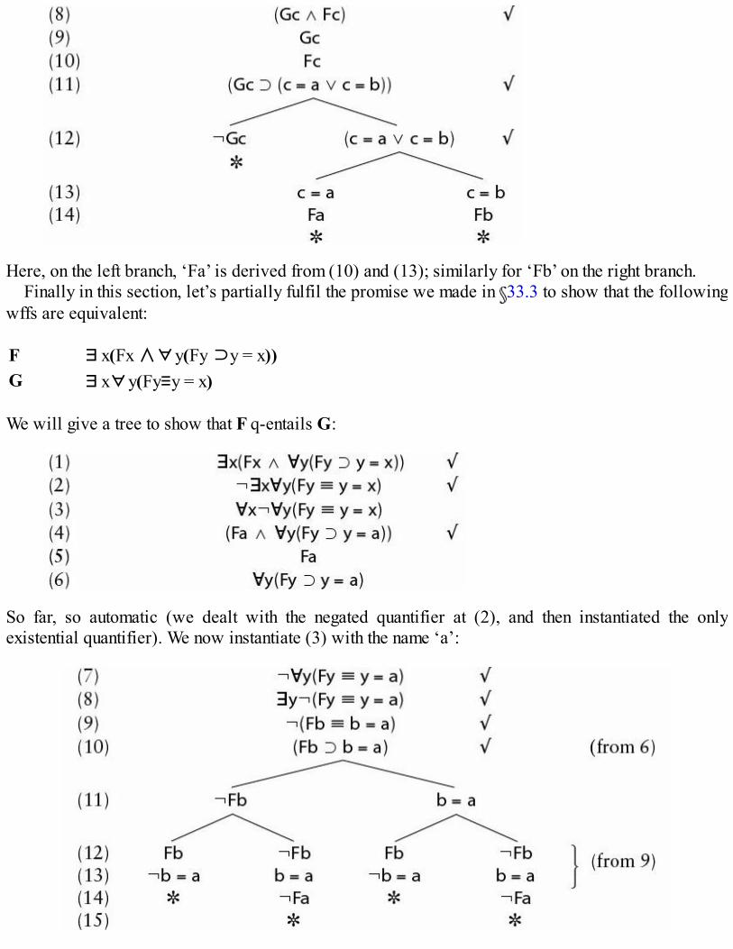
Here, on the left branch, ‘Fa’ is derived from (10) and (13); similarly for ‘Fb’ on the right branch.Finally in this section, let’s partially fulfil the promise we made in 33.3 to show that the following

wffs are equivalent:

F ∃x(Fx ∧∀y(Fy ⊃y = x))G ∃x∀y(Fy≡y = x)

We will give a tree to show that F q-entails G:

So far, so automatic (we dealt with the negated quantifier at (2), and then instantiated the onlyexistential quantifier). We now instantiate (3) with the name ‘a’:

We use (L) at line (14) to derive ‘¬Fa’ from the previous two wffs on the path: the other paths closeoff without appealing to (L). We will leave it as an exercise to show that, conversely, G q-entails F.

35.2 Self-identityConsider next the law of self identity

(Ref) ∀x x = x

This is again a q-logical truth. How can we construct a tree to show this? As usual, by assuming it isfalse on an evaluation and deriving an absurdity. Commencing the tree, we get:

Now, we haven’t yet exposed a formal contradiction in the sense of a pair of wffs of the form W and¬W. Still, getting to something of the form ¬n = n is surely just as bad! For plainly this is itself anoutright logical absurdity. Nothing can possibly fail to be identical to itself. So let’s adopt a new rulefor closing branches, which treats denials of self-identities on a par with contradictions.

Henceforth, then, our rules for QL= trees will be the QL rules, together with the new rule (L) forextending trees, and now also our new rule for closing branches – so we need to replace thestructural rule (2) given in 29.1 with this:

(2=)

Inspect any not-yet-closed path down from the top of the tree to see whether it involveseither an explicit contradiction (i.e. for some W, it contains both W and also thecorresponding formula ¬W), or a wff of the form ¬n = n. If it does, then we close that pathwith a star as an absurdity marker, and ignore it henceforth.

With our last new rule in place, we can also prove e.g. that identity obeys the symmetry law

(Sym) ∀x∀y(x = y ⊃y = x).

For consider the following tree:

Here, think of ‘¬b = a’ at (7) as being formed from a frame C (i.e. ‘¬b = _’) filled by ‘a’, and thenfrom C(a) and ‘a = b’ we get C(b) by Leibniz’s Law. We can close the tree as we’ve arrived at anabsurd denial of self-identity.

Two comments on this last proof. First, note that the wffs at lines (6) and (7), i.e. ‘a = b’ and ‘¬b =a’ are not a formal contradiction: for they are not strictly a pair of the form W and ¬W. Second, wecould have introduced a symmetry rule for identity, allowing us to move from a wff of the form m = nto one of the corresponding wff n = m. With that rule in play, we could have completed the last tree byapplying the symmetry rule to (6) to derive

and the tree would have closed off without appeal to our new closure rule. But with our new closurerule in play, an explicit symmetry rule would be redundant.

For another simple example, take the argument

H Only Bertrand is a great philosopher. Russell is a great philosopher. Hence Bertrand isRussell.

With an obvious rendition of the argument into QL=, the tree starts

Here we have completed the right-hand branch by dancing the same kind of two-step as before – i.e.we have treated ‘¬m = n’ as C(n), and used ‘n = m’ to infer the corresponding C(m), and then used our

new structural principle for closing trees.

35.3 Descriptions againIn this section, we’ll consider some arguments involving the use of Russell’s theory of descriptions.Consider firstly

I The author of the Iliad wrote the Odyssey. Homer wrote the Iliad. Hence, Homer wrote theOdyssey.

Taking ‘the author of the Iliad’ to mean ‘the person who wrote the Iliad’, this is a valid argument.Let’s use ‘F’ to render ‘wrote the Iliad’, ‘G’ for ‘wrote the Odyssey’. Then the argument can be

rendered

∃x((Fx∧∀y(Fy⊃y = x)) ∧ Gx), Fm ∴ Gm

And the corresponding tree is

Note, by the way, that had we rendered the designator ‘the author of the Iliad’ by a simpleunstructured name ‘n’ – so the first premiss is translated ‘Fn’ – we wouldn’t have been able to provevalidity.

Another example:

J Homer, and no-one else, wrote the Iliad. Homer wrote the Odyssey. Hence, the author ofthe Iliad wrote the Odyssey.

Translating, using the same key, we can start the tree

Unpacking (1) and eliminating the negated quantifier in (3), we immediately get

Instantiating the universal quantification in (6) with ‘m’ – what else? – we naturally continue

Now, we’ve almost got an explicit contradiction between the right-hand wff at (9) and (5): but notquite. ‘∀x(Fx⊃x = m)’ and ‘¬∀y(Fy⊃y = m)’ involve different variables and aren’t strictlyspeaking a pair of the form W and ¬W. If we’d had the foresight to render the initial premiss as‘(Fm∧∀y(Fy⊃y = m))’ – which would have been quite legitimate – then we would have had anexplicit contradiction by line (9). As things are, we have to continue as follows:

Instantiating (5) we have

And we are done. Note that, in this last case, we haven’t had to use the special rules for identity toshow this argument is valid. This is sometimes the way: use of the identity relation may be naturallyinvolved in the translation of the premisses and conclusion of an argument; but it may so happen thatshowing the resulting inference is q-valid only uses the fact that it is a relation and not the furtherspecial logical properties of this relation.

Here, though, is another case where we do have to appeal to the special laws of identity. Consider

K The author of the Iliad wrote the Odyssey. Hence at most one person wrote the Iliad.

According to Russell’s Theory of Descriptions, the premiss is only true if there is a unique author,and is false if there is more than one author. So, on Russell’s view, the argument is a valid one. Well,be that as it may about the vernacular argument, its closest rendition into QL= is certainly q-valid. Forconsider:

So far, we’ve unpacked (2) in automatic steps. Let’s now instantiate (1), using yet another new name,check it off and unpack the resulting triple conjunction:

Where now? Well, we plainly need to extract information from this last universal quantification. Itwould be pretty pointless to instantiate it with respect to ‘c’ (why?). But we have two other names toplay with, yielding

The right-hand branch is still open: what is there left to make use of? Well, note that at (8) we have‘¬a = b’, and now on the same branch we have both ‘a = c’, and ‘b = c’, and those wffs are clearly aninconsistent triad. Take ‘a = c’ as C(c), and use the ‘b = c’ to derive C(b) by (L), and the branchcloses thus …

We can similarly, and rather more simply, show that the following two arguments are also valid:

L The author of the Iliad wrote the Odyssey. Hence at least one person wrote the Iliad.

M The author of the Iliad wrote the Odyssey. Hence whoever wrote the Iliad wrote theOdyssey.

Those cases are left as exercises. But we will demonstrate the validity of

N A least one person wrote the Iliad. At most one person wrote the Iliad. Whoever wrote theIliad wrote the Odyssey. Hence, the author of the Iliad wrote the Odyssey.

The tree starts straightforwardly enough, following our familiar rules of thumb:

So far, so automatic. The right hand branch quickly closes, for we have

Meanwhile, the left-hand branch can be continued from (8) like this:

Inspection reveals that we haven’t yet made any appeal to (2). So let’s instantiate it with respect tothe two names in play, thus:

Once more, we arrive at a closed tree.Note, by the way, that we could put together the proofs for examples K to M to show that

(R) ∃x((Fx ∧∀y(Fy ⊃ y = x)) ∧Gx)

entails each of the conjuncts in the more long-winded triple conjunction

({∃xFx ∧∀x∀y((Fx ∧Fy) ⊃ x = y)} ∧∀x(Fx ⊃ Gy))

And the proof for N shows that this triple conjunction entails (R) – thus justifying the claim ( 34.1)that these two forms of Russell’s Theory of Descriptions for rendering ‘The F is G’ into QL= areequivalent.

35.4 ‘One and one make two’Finally in this chapter, consider the following inference:

which renders ‘There is exactly one F, there is exactly one G, nothing is both F and G, so there areexactly two things which are F or G’ (i.e. one thing and another thing make two altogether).

This inference is provably q-valid. To warrant O via a tree requires a little effort, but it is fun (of akind) to show that it can be done. We start:

First, then, eliminate the two negated quantifiers, and then instantiate the two existential quantifiers(what else?):

Now we might as well unpack the conjunctions in (7) and (8):

Next, instantiate (6) with a name, and deal with the resulting negated wff.

We now have to disentangle (15), which is a negated conjunction.

And on the rightmost branch, we obviously have to continue like this:

So far, in fact, this tree has almost written itself. We’ve applied the obvious building moves at eachstep. But now, checking back, we note that we haven’t yet made use of the two universalquantifications at (10) and (12). Instantiating (10), we can quickly close off the left of the tworemaining branches:

Phew! So the arithmetic inference O indeed turns out to be a piece of pure logic.And that is probably quite enough by way of examples of (closed) QL= trees! As for open trees,

the remarks about QL open trees in 29.3 carry over with only minor changes: to read offcountermodels from finished trees with open branches, we just must make sure that whenever wehave a wff of the form m = n on the open branch, the names involved are given the same object as q-value. But we won’t delay over this.

35.5 Soundness and completeness againFinally, we should add for the record that there is the predictable Basic Result about QL= trees too.Our collection of rules is sound and complete, so that a closed QL= tree correctly indicates a q-validargument, and there is a closed QL= tree corresponding to every q-valid argument involving identity.

To show this, we essentially need to re-run the arguments of Chapter 30. But we do need a few newtricks to handle identity, which make things just a bit more complicated. We’ll cut ourselves someslack and won’t give the details here.

35.6 SummaryWe have introduced two additional rules for quantifier tree-building, to govern trees with

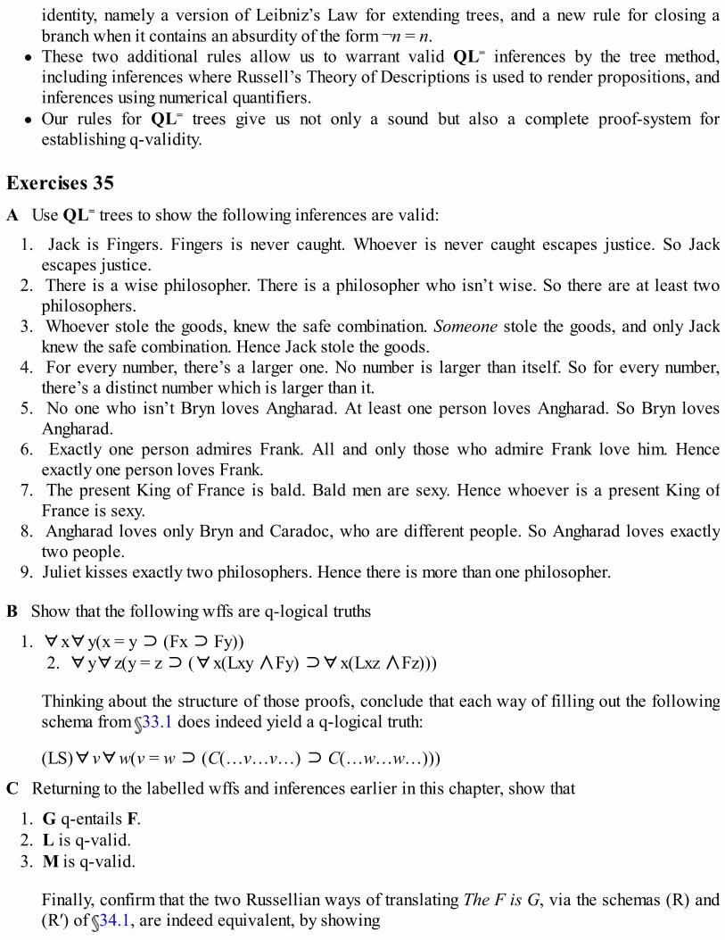
identity, namely a version of Leibniz’s Law for extending trees, and a new rule for closing abranch when it contains an absurdity of the form ¬n = n.These two additional rules allow us to warrant valid QL= inferences by the tree method,including inferences where Russell’s Theory of Descriptions is used to render propositions, andinferences using numerical quantifiers.Our rules for QL= trees give us not only a sound but also a complete proof-system forestablishing q-validity.

Exercises 35A Use QL= trees to show the following inferences are valid:

1. Jack is Fingers. Fingers is never caught. Whoever is never caught escapes justice. So Jackescapes justice.

2. There is a wise philosopher. There is a philosopher who isn’t wise. So there are at least twophilosophers.

3. Whoever stole the goods, knew the safe combination. Someone stole the goods, and only Jackknew the safe combination. Hence Jack stole the goods.

4. For every number, there’s a larger one. No number is larger than itself. So for every number,there’s a distinct number which is larger than it.

5. No one who isn’t Bryn loves Angharad. At least one person loves Angharad. So Bryn lovesAngharad.

6. Exactly one person admires Frank. All and only those who admire Frank love him. Henceexactly one person loves Frank.

7. The present King of France is bald. Bald men are sexy. Hence whoever is a present King ofFrance is sexy.

8. Angharad loves only Bryn and Caradoc, who are different people. So Angharad loves exactlytwo people.

9. Juliet kisses exactly two philosophers. Hence there is more than one philosopher.

B Show that the following wffs are q-logical truths

1. ∀x∀y(x = y ⊃ (Fx ⊃ Fy))2. ∀y∀z(y = z ⊃ (∀x(Lxy ∧Fy) ⊃∀x(Lxz ∧Fz)))

Thinking about the structure of those proofs, conclude that each way of filling out the followingschema from 33.1 does indeed yield a q-logical truth:

(LS)∀v∀w(v = w ⊃ (C(…v…v…) ⊃ C(…w…w…)))

C Returning to the labelled wffs and inferences earlier in this chapter, show that

1. G q-entails F.2. L is q-valid.3. M is q-valid.

Finally, confirm that the two Russellian ways of translating The F is G, via the schemas (R) and(R′) of 34.1, are indeed equivalent, by showing

4. ‘∃x∀y((Fy≡y = x) ∧Gx)’ q-entails ‘∃x((Fx ∧∀y(Fy ⊃ y = x)) ∧Gx)’.5. ‘∃x((Fx ∧∀y(Fy ⊃ y = x)) ∧Gx)’ q-entails ‘∃x∀y((Fy≡y = x) ∧Gx)’.

36

Functions

One of the first quantificational formal languages that you are likely to meet if you go on to slightlymore advanced work on logic is the language of arithmetic. And this – as you would expect – hassymbols for e.g. the addition and multiplication functions. So it would be odd to leave ourintroductory exploration of quantificational logic without briefly saying something about how toextend the language QL= to include such expressions for functions. Our discussion will also give usanother angle on the theory of descriptions.

36.1 Functions re-introducedWe’ve already touched on the basic idea of a function in 11.2. A function maps an object or objectsto some unique thing. For example, ‘the age in years (at January 1, 2009) of x’ expresses a functiondefined over living people, correlating each person with a single number. And ‘the product of x and y’expresses a function defined over numbers, correlating two numbers with another number.

Let’s quickly review an assortment of elementary points about functions, and fix nomenclature andinformal notation.

We call the input(s) to a function – the object(s) to which the function is applied – theargument(s) of the function. The unique output of the function for given argument(s) is the valueof the function. For example, the number 35 is the value of the function the age in years (atJanuary 1, 2009) for the argument Gwyneth. The number 35 is also the value of the productfunction for the arguments 5 and 7.The value of a function can be a quite different sort of entity from the argument: 35 is a number,Gwyneth is a woman. But of course the value can equally well be the same sort of thing as theargument(s): the product function maps numbers to numbers.A function can have more than one argument. For example, the arithmetical addition andmultiplication functions each take two arguments. Or consider the family of truth-functions. Thematerial conditional, for example, maps two truth-values (those of its antecedent andconsequent) to a truth-value; the trumped-up $ truth-function of 11.7 takes three truth-values asarguments; etc.Mathematicians notationally represent functions in various ways. For instance, the square rootfunction is expressed by the special prefixed symbol in ‘√9’; the product function is usuallyexpressed by the ‘infix’ multiplication symbol, i.e. the symbol placed in the middle of ‘5 × 7’;and the square function is indicated by the ‘postfix’ superscript in ‘92’. But the generic way ofrepresenting functions is by symbolism like ‘f( )’ or ‘g( , )’ etc., with one or more slots waitingto be filled in by designators for the arguments. Suppose that ‘f( )’ expresses the function thatmaps a number to its square. Then ‘f(2)’ is a complex designator denoting the number 4, ‘f(7)’

denotes 49, and so on. Likewise, if ‘g( , )’ expresses the product function, then ‘g(5, 7)’ denotesthe number 35.When an argument and value are objects of the same kind, we can apply that function again to theresults of previous applications. Thus ‘f(f(2))’ denotes the square of f(2), i.e 16. Similarly,‘g(f(2), f(3))’ denotes 36.

So far, so elementary! Now for two further points that will need more careful explanation. First,

We must distinguish the sense or interpretation of a function expression from its extension; thelatter is what fixes the truth-value of sentences involving the function expression.

Compare our distinction between the sense and extension of predicates ( 30.1). The sense is what isgrasped by someone who understands the predicate; but it is the extension which fixes the truth-valuesof sentences involving the predicates (if we forget about intensional contexts). Similarly here: thesense of a function sign is what you have to grasp in order to count as understanding the expression.We can typically think of this as a rule or procedure for correlating objects with other objects. Forexample, to grasp the sense of ‘square of ( )’, you need to understand the rule that we arrive at thevalue of the function for argument n by multiplying n by itself. The rule determines a set of pairings ofarguments and values, thus {0, 0, 1, 1, 2, 4, 3, 9, 4, 16, …}. This set of pairs isthe extension of the function.

Just as two predicate expressions can have different senses but the same extension, so too forfunction expressions. Here’s a very simple arithmetical example. Consider ‘(x + 1)2’ and ‘x2 + 2x +1’. These expressions have different senses, for they indicate different calculation procedures forassociating values with arguments. However, the resulting argument-to-variable pairings are thesame.

We needn’t argue about whether the word ‘function’ is ordinarily used to talk of a mappingprocedure or to talk of the resulting pairings of arguments and values. What matters is that we note therelevance of the sense/extension distinction here. The extension of a function is what fixes truth-values. For example, ‘f(m) = n’ is true if the pair m, n is in the extension of ‘ f’; ‘For all x, f(x) >x’ is true if for any pair m, n in the extension of ‘ f ’, n > m. And so on.

Finally, note that even when a rule for processing an argument is well-defined across some domain,it may not always deliver a value. Take for example the eldest-son-of function. The rule for getting avalue can be applied to any adult human: we look to see whether he or she has sons, and if so pick outthe eldest. But this procedure may well deliver a null return. Compare the square-of function: takeany integer as argument and this function always delivers a value. We therefore need to note thefollowing distinction:

Some functions are total functions, i.e. have a value for all arguments from the relevant domain.Others are strictly partial functions, which have no value for certain arguments.

36.2 Adding functions to QL=

It is syntactically pretty straightforward to add function expressions to QL=. And it is semanticallyunproblematic too, so long as we restrict ourselves to total functions defined over the wholedomain, with values in that domain (the real significance of this restriction will become clear in 36.4). An outline sketch of the resulting language QLf will suffice.

So, first we’ll want to add to QL=’s vocabulary some function expressions taking various numbersof arguments. We can start off with ‘naked’ lower case letters like ‘f’, ‘g’, ‘h’, …. (And then, if wewant to ensure we don’t run out of possible function expressions, we can again use superscripts andsubscripts, so is the kth j-argument function symbol.)

We will next need to complicate our definition of a term (compare 26.3).

(1) An individual constant or individual variable is a term.(2) If f is a function symbol taking one argument and t is a term, then f(t) is a term. More generally,

an n-argument function symbol followed by a left-hand bracket, following by n terms (separatedby commas), followed by a right-hand bracket, is also a term.

(3) Nothing else is a term.

This allows expressions like the following to count as terms:

f(m), f(y), g(m, n), g(x, f(m)), g(f(y), f(m)), g(g(m, n), f(m)), …

If a term doesn’t include any variables, it is a closed term (compare the idea of a closed wff, 26.4).The syntactic rules for building up wffs can stay as before, except that ‘atomic wff’ is now perhaps

something of a misnomer for the basic building block wff consisting of an n-place predicate followedby n terms, given that the terms can themselves be quite complex.

By the way, it is worth commenting that the use of bracketing and commas here in our notation forfunctions is strictly speaking redundant. However, it is absolutely standard (and you can easily seewhy: bracket-free expressions like ‘ggmnfm’ are horribly unreadable).

Now for the semantics. Start with the simplest case, a one-argument function. A q-valuation willassign this function a set of ordered pairs of objects (i.e. the pairs of argument and value), wherethese objects are both from the domain (they need to be among the things that count as ‘everything’).This set of pairs must have the following two features:

i. For each object m in the domain of discourse, there is some pair m, o in the extension, i.e.a pair whose first member is m.

ii. It contains no distinct pairs m, o and m, o′, where o differs from o′.

(i) must hold given we are currently restricting our attention to total functions.(ii) must hold because a function relates an object as argument to a unique object as value.

Similarly for a two-argument function. A q-valuation will assign this sort of function a set ofordered triples of objects from the domain. This set must have the following two features:

i′. For each pair of objects m, n in the domain of discourse – which serve as arguments to thefunction – there is some triple m, n, o in the extension .

ii′. It contains no distinct pairs m, n, o and m, n, o′, where o differs from o′.

The generalization to cover functions with n arguments is straightforward.The next stage in setting up the semantics is to give rules for evaluating terms including function

expressions. The basic idea is very simple. Suppose a q-valuation already assigns ‘m’ the object m asreference. And suppose that on the same q-valuation, the pair m, o is in the extension of the one-place ‘f’ (intuitively, the function maps m to o). Then the q-value of the term ‘f(m)’ is of course o.

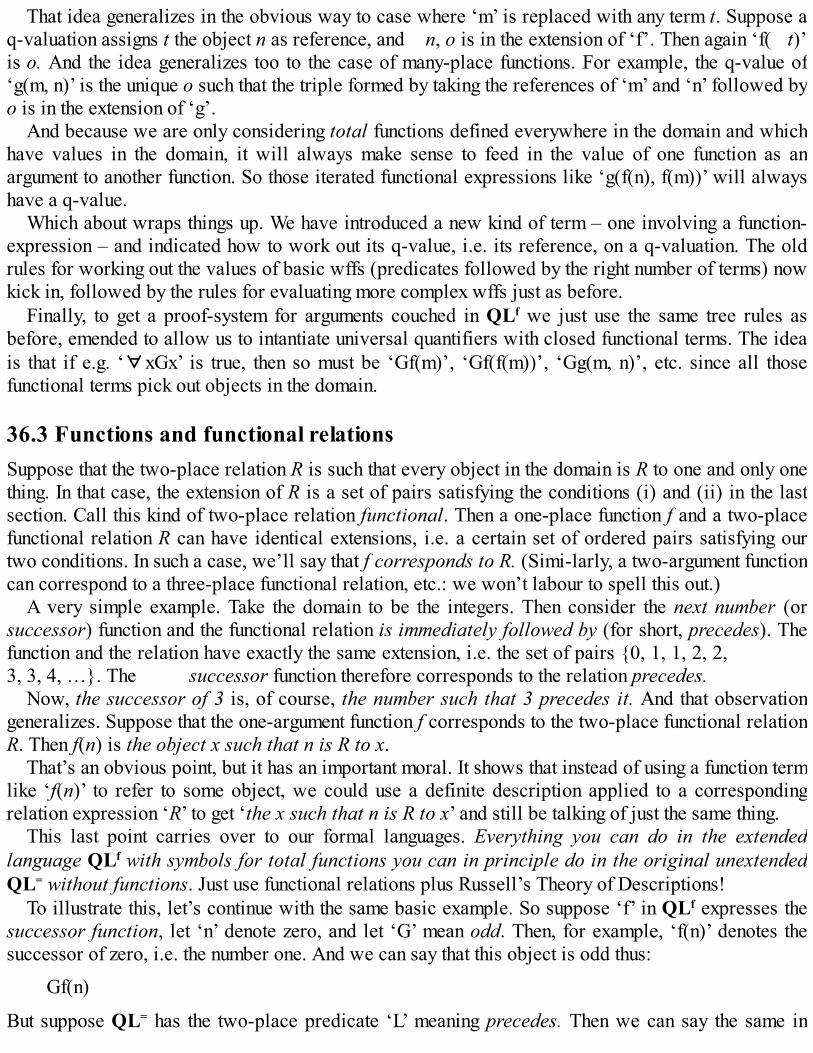
That idea generalizes in the obvious way to case where ‘m’ is replaced with any term t. Suppose aq-valuation assigns t the object n as reference, and n, o is in the extension of ‘f’. Then again ‘f( t)’is o. And the idea generalizes too to the case of many-place functions. For example, the q-value of‘g(m, n)’ is the unique o such that the triple formed by taking the references of ‘m’ and ‘n’ followed byo is in the extension of ‘g’.

And because we are only considering total functions defined everywhere in the domain and whichhave values in the domain, it will always make sense to feed in the value of one function as anargument to another function. So those iterated functional expressions like ‘g(f(n), f(m))’ will alwayshave a q-value.

Which about wraps things up. We have introduced a new kind of term – one involving a function-expression – and indicated how to work out its q-value, i.e. its reference, on a q-valuation. The oldrules for working out the values of basic wffs (predicates followed by the right number of terms) nowkick in, followed by the rules for evaluating more complex wffs just as before.

Finally, to get a proof-system for arguments couched in QLf we just use the same tree rules asbefore, emended to allow us to intantiate universal quantifiers with closed functional terms. The ideais that if e.g. ‘∀xGx’ is true, then so must be ‘Gf(m)’, ‘Gf(f(m))’, ‘Gg(m, n)’, etc. since all thosefunctional terms pick out objects in the domain.

36.3 Functions and functional relationsSuppose that the two-place relation R is such that every object in the domain is R to one and only onething. In that case, the extension of R is a set of pairs satisfying the conditions (i) and (ii) in the lastsection. Call this kind of two-place relation functional. Then a one-place function f and a two-placefunctional relation R can have identical extensions, i.e. a certain set of ordered pairs satisfying ourtwo conditions. In such a case, we’ll say that f corresponds to R. (Simi-larly, a two-argument functioncan correspond to a three-place functional relation, etc.: we won’t labour to spell this out.)

A very simple example. Take the domain to be the integers. Then consider the next number (orsuccessor) function and the functional relation is immediately followed by (for short, precedes). Thefunction and the relation have exactly the same extension, i.e. the set of pairs {0, 1, 1, 2, 2,3, 3, 4, …}. The successor function therefore corresponds to the relation precedes.

Now, the successor of 3 is, of course, the number such that 3 precedes it. And that observationgeneralizes. Suppose that the one-argument function f corresponds to the two-place functional relationR. Then f(n) is the object x such that n is R to x.

That’s an obvious point, but it has an important moral. It shows that instead of using a function termlike ‘f(n)’ to refer to some object, we could use a definite description applied to a correspondingrelation expression ‘R’ to get ‘the x such that n is R to x’ and still be talking of just the same thing.

This last point carries over to our formal languages. Everything you can do in the extendedlanguage QLf with symbols for total functions you can in principle do in the original unextendedQL= without functions. Just use functional relations plus Russell’s Theory of Descriptions!

To illustrate this, let’s continue with the same basic example. So suppose ‘f’ in QLf expresses thesuccessor function, let ‘n’ denote zero, and let ‘G’ mean odd. Then, for example, ‘f(n)’ denotes thesuccessor of zero, i.e. the number one. And we can say that this object is odd thus:

Gf(n)

But suppose QL= has the two-place predicate ‘L’ meaning precedes. Then we can say the same in

QL= by translating ‘The number such that zero precedes it is odd’. Applying the familiar Russellianschema, we’ll get

∃x((Lnx ∧∀y(Lny ⊃ y = x)) ∧Gx)

Likewise, have the following mappings from QLf wffs to QL= equivalents:

∃zGf(z) ∃z∃x((Lzx ∧∀y(Lzy ⊃ y = x)) ∧Gx)f(n)= m ∃x((Lnx ∧∀y(Lny ⊃ y = x)) ∧x = m)∀z(Gz ⊃f(z)= m) ∀z(Gz ⊃∃x((Lzx ∧∀y(Lzy ⊃ y = x)) ∧x = m))

and so on and so forth.Now, it is already clear that there is a real gain in clarity in having the function symbolism

available. The gain is very substantial when there’s more than one functional symbol to be translatedaway at the same time. Take for example the simple claim that addition in arithmetic is symmetric, i.e.for all x and y, x + y = y + x. This goes into standard QLf simply enough as something like

∀x∀y(h(x, y) = h(y, x))

if we use ‘h’ for the two-argument sum function. Or we may simply allow ourselves to borrow thefamiliar infix arithmetical function symbols in an extension of QL= so we can write

∀x∀y(x + y = y + x)

But suppose we try to manage instead in unaugmented QL=, using the three-place sum relation ‘S’,where ‘Smno’ means m + n = o. Then to express the symmetry of addition we need, informally,

∀x∀y(the v1 such that Sxyv1 = the v2 such that Syxv2)

Getting rid of the two descriptions now introduces another four quantifiers:

which is a lot less perspicuous!

36.4 Partial functions and free logicIn the light of what we’ve just said, the question whether to expand QL= to QLf really comes down tothe question of how important it is for us to have a logical formalism which can deal briskly andperspicuously with total functions (recall: QLf only deals with total functions). It is a trade-offbetween economy of resources and ease of manipulation.

But now it is worth stressing again that many functions are strictly partial. They abound inmathematics: to take the very simplest case, the division function doesn’t deliver a value everywhere(there is no output when you divide a number by zero).

You might wonder whether partial functions are much of an issue. To be sure, some definitions onlycharacterize partial functions, like the definition of division. However, can’t we just (as it were) fill

up the gaps in a partial function by arbitrary stipulation? For example, we could define the totaldivision* function, where m divided* by n is the same as m divided by n when n > 0, and is equal to(say) 0 when n is 0. And we could stipulate that the eldest son* function has the same value as theeldest son function when that has a value but outputs (say) the number 0 as a default in other cases.So, when we want to be logically tidy, can’t we pretend all our functions are ‘completed’ in this sortof way?

Unfortunately, wishing away partial functions doesn’t work. It is, for example, a fairly elementaryresult in the theory of computation that you can have a partial function f which is computable – i.e.there is a computer program that works out the value of f for every argument for which it is defined –but f ’s completion-by-stipulation yields a total function f* which is not computable by any possibleprogram. Moral: a general theory of functions has to take partial functions seriously. In short, if wewant to treat functions in a logical system, the natural aim will be to cover all functions, total andmerely partial.

So suppose now, to return to an earlier example, that ‘s( )’ expresses the partial eldest-son-offunction. Suppose too that ‘m’ denotes George Bush Snr., ‘n’ denotes Hillary Clinton, and ‘F’ means ismale. We will take the domain to be people. Then ‘s(m)’ is unproblematic: it is a term denotingGeorge W. Bush, and ‘Fs(m)’ straightforwardly evaluates as true.

What about ‘s(n)’? Hillary has no son, so this denotes no one, and ‘s(n)’ has no q-value. So whatshould we say about the value of ‘Fs(n)’? A wff consisting of a predicate followed by a term is onlytrue if the q-value of the term is in the extension of the predicate. So such a wff is certainly not true ifthe term lacks a q-value. Does that mean (1) that ‘Fs(n)’ is false? Or does it mean (2) that it lacks atruth-value?

Either option is technically workable, and we get two versions of free logic – i.e. a logic which isfree from the assumption that all closed terms (terms without free variables) denote. But option (2) isarguably more natural. For if we have no general beef against the idea of partial functions, then it ispretty unclear why we shouldn’t allow partial evaluation functions too, and hence allow some wffs tocome out neither true nor false. However, allowing such truth-value gaps will force major revisionsin the very fundamentals of our formal logic. For example, even instances of (A ∨¬A) needn’t alwaysbe true, at least if we keep the traditional truth-tables: replace A with a wff which is neither true norfalse and the disjunction will lack a truth-value too.

Option (1) is in some ways less radical. On this line, all wffs remain either true or false. But wewill still have to revise our logic. For a start, in our example, we could have ‘∀xFx’ true but ‘Fs(n)’is false. So we now can’t always instantiate universal quantifications with functional terms.

So in fact either version of free logic we have mentioned will be revisionary of the logic of QLf.Moreover, once we allow non-denoting functional terms, it is difficult to see why we shouldn’t allownon-denoting names as well, a further departure into a thoroughly free logic.

The situation in sum is this: QLf is an extension of QL=, which gives us a neat, brisk representationof total functions defined over a domain, more manageable than dealing with functions via definitedescriptions applied to functional relations. However, the restriction to total functions is ratherunnatural (though it enables us to preserve ‘classical’, two-valued logic). Going any further, andtaking partial functions seriously, requires significant innovations.

But we can’t explore these matters any further here, except to conclude by revisiting the issue of …

36.5 Definite descriptions again

Russell, we noted, held that his Theory of Descriptions in some sense revealed the true logical formof our everyday sentences involving definite descriptions. It is far from clear what the cash value ofsuch a claim is. Still, we are now in a position to make some pertinent comments.

Recall the very close connection between functions and descriptions noted in 36.3. We saw thatthe successor function, for example, can be defined by applying a definite description operator (a‘the’ operator) to the predecessor relation. Or consider Russell’s own paradigm example ‘the(present) King of France’ again. This invites treatment as a functional term, denoting the value of thethe king of function for the argument France. And ‘the king of …’ can, in turn, be thought of asequivalent to ‘the x such that x is king of …’ – i.e. as defined in terms of a ‘the’ operator applied to atwo-place functional relation ‘… is king of …’.

Suppose that we are dealing with a language which has expressions for both functions andfunctional relations. Then it is very natural to add a ‘the’ operator for making functions out offunctional relations. In 36.3, we were talking about how we might do without functions by usingfunctional relations instead; now we are considering how to move between relations and functionswhen you do have both in the language.

Let’s use the symbol ‘ι’ for our the operator – that’s a Greek letter iota, which is traditional for adescription operator, following Russell (though we certainly don’t want to get sidetracked here into adiscussion of the nuances of various uses of the iota symbol in the literature). The basic idea,therefore, will be that the ι-operator applied to an n + 1 place functional predicate R yields thecorresponding function of n arguments. And the natural way of implementing the idea is to make ‘ι’ avariable-binding operator akin to a quantifier. In other words: we use ‘ι’ with the variable ‘x’ or ‘y’or …, and this ties it to a slot in R with the same variable in it.

For example, take the two place functional relation ‘L’. Then

ιyLxy

means the thing y such that x has relation L to y. ‘ιyLxy’ is therefore a one-place functionalexpression that works like ‘f(x)’ (it lacks the brackets, but then the brackets we usually use withfunction expressions are only there to promote readability). If we replace the free variable with aconstant as in

ιyLmy

we get a term that works like ‘f(m)’.Four observations. (1) If we are still working in the context of QLf, then operators have to be

applied with care to make sure that the resulting functions indeed exist as total functions. But if wesuppose now that we are working in the context of a free logic which allows partial functions, then –if you will excuse the pun – we can be much more free in the use of our new operator.

(2) We said that applying the ι-operator to an n+1 place relation yields an n-place function. Let’sallow the case where n = 0. So applying the same ι-operator to a one place predicate yields a termwith zero slots left to be filled up – ‘ιxFx’ just serves to designate the x which is F. So, the ι-operatoris also a way of forming definite description terms out of monadic predicates.

(3) Since ‘ιxFx’ is like a closed term, ‘GιxFx’ is a sentence. And in some appropriate logicalsystems for a description operator – including some versions of free logic – we will be able to showthat

(F) GιxFx

(i.e. the thing which is F is G) is true in a valuation if and only if

(R) ∃x(Fx ∧ (∀y(Fy ⊃ y = x) ∧Gx))

is also true.(4) That shows that, even if Russell is right that the rendition (R) has the same truth-conditions as

‘The F is G’, it doesn’t mean that he is right that descriptions are fundamentally some kind ofquantifier. It could be that the description-former ‘the’ in natural language often works like the ‘ι’-operator, i.e. not as a quantifier but as a function-forming operator on relations. In other words,perhaps (R) has the same truth-conditions as ‘The F is G’ as a consequence of descriptions workingon the functional model, rather than because (R) itself reflects the correct story about the ‘logicalform’ of sentences with descriptions.

However, we can’t pursue this suggestion any further here. The issue of the proper treatment ofdefinite descriptions remains contentious a century after Russell first proposed his treatment. Whichis a salutary closing reminder that issues in logic are not always as cut-and-dried as text books – likethis one! – can make them seem.

36.6 SummaryWe could also extend QL= to include expressions for functions. The simplest extension, QLf,only allows expressions for total functions (i.e. functions that have a value for all arguments inthe domain).The logic of QLf is not very different to that of QL=, and it allows a much more economictreatment of functions compared with using functional relations and the theory of descriptions inQL=.However, QLf is arguably an unstable compromise: if we are going to treat functions, shouldn’twe also treat partial functions (i.e. functions that do not deliver a value for all arguments in thedomain)?To cope with partial functions, and hence the use of terms which lack reference, will meanadopting some kind of free logic, which will have significantly different logical laws from thosethat govern QL=.In a language which has functions, we could introduce a ι-operator (read ‘the’) that takes us froman n + 1-place predicate to a corresponding n-place function. Arguably, the vernaculardescription-forming operator ‘the’ works similarly.

Further reading These notes on further reading are divided into two parts. The first section lists references that aredirectly tied to points arising in the body of the book; the second suggests some text books for paralleland more advanced reading.

Matters arisingOn the nature of propositions ( 2.5), see

A. C. Grayling, An Introduction to Philosophical Logic (Blackwell, 3rd edn. 1997), Ch. 2.

Quine-quotes ( 10.3) are introduced in

W. V. O. Quine, Mathematical Logic (Harper and Row, 2nd edn. 1951), 6;

they are also well explained e.g. by

Graeme Forbes, Modern Logic (Oxford U.P., 1994), Ch. 2, 6.

Real enthusiasts might be amused by

George Boolos, ‘Quotational ambiguity’, in his Logic, Logic, and Logic (Harvard UP, 1988).

On the ideas of necessity, analyticity and the a priori ( 12.5), see

A. C. Grayling, An Introduction to Philosophical Logic, Ch. 3.

On the troublesome question of the meaning of ‘if’ (Chapters 14, 15), see

Frank Jackson, ed., Conditionals (Oxford UP, 1991). Frank Jackson, Conditionals (Blackwell, 1987).

The first of these books is a reader, collecting together a number of key papers on the interpretation ofconditionals (read V. Dudman’s concluding contribution if you aren’t yet persuaded of thecomplexities of the behaviour of conditionals). The reader reprints a paper by the Jackson himself,which proposes his ‘robust material conditional’ story about the meaning of indicative ‘ifs’ ( 15.4).This is developed in his own extremely readable short book. Our example ‘If kangaroos had no tails,they would topple over’ ( 15.1) is borrowed from the opening section of a modern classic,

David Lewis, Counterfactuals (Blackwell, 1973).

We said in 20.3 that tree proofs can sometimes be radically shortened by adopting the (evidentlysound) rule that at any point you can add an instance of the law of excluded middle, i.e. a wff of theform (C ∨ ¬C). For discussion, see

George Boolos, ‘Don’t eliminate cut’, in his Logic, Logic, and Logic.

For further discussion of the motivation for the quantifier-variable notation for generality ( 21.4),

see another modern classic,

Michael Dummett, Frege: Philosophy of Language (Duckworth, 2nd edn. 1981), Ch. 2.

We mentioned in passing ( 23.4) that with a bit of cunning we can do without variables (whileretaining the key idea that quantifiers are operators that are applied to predicates, and are quitedifferent from names). For more on this, see

W. V. O. Quine, ‘Variables explained away’, in his Selected Logic Papers (Harvard UP, 1995).

On Frege’s claim that names have sense as well as reference ( 31.1), see the much-reprinted

Gottlob Frege, ‘On sense and reference’ – or, as it is called in his Collected Papers (Blackwell,1984), ‘On sense and meaning’.

For a lively challenge to the conventional wisdom about how we can substitute co-referential namesin ‘simple’ contexts, see

Jennifer M. Saul, ‘Substitution and simple sentences’, Analysis 57 (1997), pp. 102–108.

For Russell’s Theory of Descriptions ( 34.1), see the essays in

Gary Ostertag, ed., Definite Descriptions (MIT Press, 1998)

especially Chs. 3 (Russell’s own statement), 8 and 11. And for a little on free logic ( 34.4), see

Graham Priest, An Introduction to Non-Classical Logic (Cambridge UP, 2nd edn. 2008), Ch. 13.

Other textsA Parallel reading For a classic text which covers similar ground to this present book, see

Richard Jeffrey, Formal Logic: Its Scope and Limits (McGraw-Hill, 3rd edn. 1990).

Another much used student text (which also concentrates on trees but goes rather more slowly thanJeffrey) is

Wilfrid Hodges, Logic (Penguin, 2nd edn., 2001).

B Some introductory texts that range more widely Three more good texts (at about the same level ofdifficulty as this book) which cover natural deduction proofs as well as trees are

Merrie Bergmann, James Moor and Jack Nelson, The Logic Book (McGraw-Hill, 3rd edn. 1998).

Graeme Forbes, Modern Logic (Oxford UP, 1994)

Paul Teller, A Modern Formal Logic Primer (Prentice Hall, 1989).

Teller’s text is in two volumes but don’t be put off by that: it is in fact quite short, and has aparticularly approachable, relaxed style. The bad news is that it is out of print; the good news is thatan electronic version is freely available at the book’s website, http://tellerprimer.ucdavis.edu.

But the best introduction to natural deduction is probably the elegant and sophisticated

Neil Tennant, Natural Logic (Edinburgh UP, 2nd edn. 1990).

While Teller, for example, presents a linear natural deduction system with indented subproofs,

Tennant goes straight for downwards-joining tree deductions (see our 20.1).

C Going further in first-order logic Two good places to start are

David Bostock, Intermediate Logic (Oxford UP, 1997)

Ian Chiswell and Wilfrid Hodges, Mathematical Logic (Oxford UP, 2007).

Despite their titles, neither book goes a great deal further than this one. But Bostock is very good onthe motivations for varying styles of logical system, on the relations between them, and on explainingsome key proof ideas. Chiswell and Hodges is also very clear and gives an excellent basis for moreadvanced work.

A classic text that has to be mentioned here is the wonderful

Raymond Smullyan, First-Order Logic (Springer-Verlag, 1968: Dover, 1995).

But this isn’t easy, as it packs a great deal into just over 150 pages; but at least read the first third tosee where all our work on trees in this book ultimately comes from. Another text that is elegantlydone and, like Smullyan, pushes well beyond the bounds of this book is

Dirk van Dalen, Logic and Structure (Springer-Verlag, 4th edn. 2004).

These two books should particularly appeal to the mathematically minded.

D Extending classical logic One or twice, we’ve mentioned modal logic, i.e. the logic of necessityand possibility. Three recent texts worth looking at (the third is based very much on trees) are

J. C. Beall and Bas C. van Fraassen, Possibilities and Paradox (Oxford UP, 2003).Rod Girle, Modal Logics and Philosophy (Acumen, 2000). Graham Priest, An Introduction to Non-Classical Logic, Chs 2, 3.

Another standard text is

Brian Chellas, Modal Logic: An Introduction (Cambridge UP, 1980).

The formal and philosophical aspects of second-order logic (where we quantify over properties aswell as things) are discussed in the terrific

Stewart Shapiro, Foundations without Foundationalism (Clarendon Press, 1991).

And for much, much more, see the (mostly excellent) survey articles in the four volumes of thesomewhat mistitled

D. Gabbay and F. Guenthner, eds., A Handbook of Philosophical Logic (D. Reidel. 1983–89).

E Philosophical logic Returning now from more advanced technicalities to philosophicalcommentary on the sort of formal logic covered in this book, the place to start has to be

Mark Sainsbury, Logical Forms (Blackwell, 2nd edn. 2000).

Each chapter ends with an extraordinarily helpful guide through the complications of the relevantliterature, and we need not repeat those guides here.

IndexSome standard logic symbols

∧, 59∨, 59¬, 59∴, 63, 73, 101

, 63, 149&, 70∼, 70⊃, 70, 127–128→, 70, 135

, 86↓, 98↑, 99|, 99

, 118≡, 132⊥, 144

, 190∀, 200, 204∃, 200, 204

257–258=, 304, 309≠, 311!, 313

, 320ι, 345

Some other symbols special to this book

⇒, 75⊕, 95

, 220⇒q, 257

∀-instantation rule, 230, 279–282a priori vs. a posteriori, 104alphabet

of PL, 63of PLC, 133of QL, 245of QL=, 309

analytic vs. synthetic, 105antecedent, 126argument, 1

by cases, 129deductive, 4inductive, 4multi-step, 37, 47–49reductio, 39–40schema, 6sound, 14valid, 13–14

Aristotle, 28, 32–33, 58, 101, 216atomic wff

of PL, 60, 63–64of PLC, 133of QL, 202, 245of QL=, 309

‘bad line’, 111Basic Result

for PL trees, 160, 179–182for PLC trees, 171for QL trees, 286for QL= trees, 337

Beall, J., 350Bergmann, M., 350biconditional, 131

material, 132Boolos, G., 190, 348, 349Bostock, D., 350

Carroll, L., 8, 34, 36, 37Chellas, B., 350Chiswell, I., 350classical propositional logic, 124classical validity, see validityclosed

path, 158tree, 160, 330wff, 248

completeness, 182, 191, 280, 287–291conclusion, 2, 7, 15conditional

counterfactual, 138‘Dutchman’, 142–143material, 128Philonian, 128possible-world, 137subjunctive, 138truth-functional, 126–128

conjunction, 55basic, 95–96

connective, 55, 203, 207binary, 64main, 67truth-functional, 88–90

consequent, 126consistency

logical, 10syntactic, 183, 288

constant, 202, 245, 251construction tree, 66–67, 77, 246contingent truth, 104contradiction, 40, 101–102counterexample, 31, 118

technique, 31–32countermodel, 263, 267–269

De Morgan’s Laws, 100deductive argument, 4

one-step, 13–14

multi-step, 47–49valid, 4

definite description, 316Russell’s Theory, 317, 331–335, 343, 345–346scope, 319–320

designator, 306, 316disjunction

exclusive vs. inclusive, 56, 95disjunctive normal form, 97–8disjunctive syllogism, 149domain of discourse, 205, 251

empty, 251, 280Dudman, V., 348Dummett, M., 349

∃-instantation rule, 236elimination rule, 188entailment

logical, 4tautological, 108see q-entailment

enthymeme, 39equivalence

class, 305relation, 304truth-functional, 94, 120, 134–135see q-equivalence

excluded middle, 101existence statements, 322–324existential import, 214existential quantifier, 204expressive adequacy, 97extension of predicate, 252, 296

vs. meaning, 297extensional context, 298extremal clause, 64

fallacyaffirming the consequent, 130denying the antecedent, 130of irrelevance, 46quantifier-shift, 33

falsum, 144first-order vs. second-order, 311, 350Forbes, G., 348, 349form

of inference, 6, 19–27logical, 25–27, 103–104, 215–217, 318–319, 321and validity, 26, 117, 266, 295

formal language, 58free logic, 323, 344–345free variable, 244, 248, 254Frege, G., 58, 297, 300, 349function, 89, 339–346

argument, 339extension, 340partial, 341, 344–345vs. relation, 342

total, 341value, 89, 339see truth-function

Gabbay, D., 351Girle, R., 350Gödel, K., 270Grayling, A., 348Guenthner, F., 351

Hodges, W., 349, 350hypothetico-deductive model, 11–12

iff, 131implication

logical vs. material, 134identity

of indiscernibles, 306numerical, 303qualitative, 303see Leibniz’s Law

indiscernibility of identicals, 306individual

constant, 202, 245, 251variable, 200, 245

inductive argument, 4, 45inference, 2

pattern, see form of inferenceto the best explanation, 10–11valid, 4, 13

infinitecountermodel, 268–269, 284tree, 239–240, 291–292see König’s lemma

informal logic, 34, 52intensional

context, 298vs. intentional, 301

interpretationof PL wffs, 72–73of QL wffs, 203–207vs. valuation, 75, 250–251, 296–297

introduction rule, 188intuitionistic logic, 164invalidity principle, 13

Jackson, F., 141, 348Jeffrey, R., 177, 349

König’s lemma, 291

languageformal, 58object, 83see metalanguage

law,de Morgan’s, 100excluded middle, 101

non-contradiction, 101see Leibniz’s Law

Leibniz, G., 306Leibniz’s Law, 306, 310, 325–326Lewis, D., 137, 349logical form, see formlogically consistent, 10logically possible, 10

main connective, 67main logical operator, 247material

biconditional, 132conditional, 128, 137–143implication, 134

mechanical technique, 5, 42, 64, 65, 90, 101, 108, 115, 124, 240, 269–270metalanguage, 83metalogical results, 95, 119, 134, 179– 184, 259–260, 286–293modal

context, 301–302logic, 197, 217, 350operator, 197, 320

model, 262modus ponens, 126modus tollens, 126Moor, J., 350

name, 199, 202,empty, 323scopeless, 199see constant

nameless things, 207natural deduction, 37, 187–188necessary

condition, 132truth, 104–106

negation, 57Nelson, J., 350node (of tree), 157

object language, 83‘only if’, 131open

path, 158tree, 160, 240, 282–284wff, 248

Ostertag, G., 349

path (on tree), 157closed vs. open, 158satisfiable, 179, 286

Philo, 128PL,

design brief, 59rules (for trees), 159semantics, 72–76syntax, 63–65tree, 151–170

PLC, 132–133rules (for trees), 172tree, 171–176

PLF, 144Plato, 38possibility, 9–10

see necessary truthpossible worlds, 12, 104, 137, 302predicate, 18, 202, 245

extension of, 252logic, 192

premiss, 2, 7, 15suppressed, 39

Priest, G., 349, 350proposition, 15–16

atomic, 60propositional logic, 124proof, 37

annotated, 38, 65downward-joining tree, 66, 185downward-splitting tree, 66, 185–187

q-entailment, 262q-equivalence, 313q-logical truth, 263, 322–323q-validity, 193, 250–251, 262, 266–267q-valuation, 250–253q-value,

of constant, 251of predicate, 252

QLatomic wff, 202individual constant, 202individual variable, 204predicate, 202quantifier, 204semantics

informal, 203–206official, 253, 256–257

syntaxinformal, 202–205official, 245

tree, 228–240, 265–266, 272–285QL=

syntax, 309semantics, 309–310tree, 325–336

QLf, 341–342quantifier, 33, 194–201, 204

existential, 204numerical, 313–314restricted, 211–213substitution instance, 208, 248universal, 204

quantifier-shift fallacy, 33‘quantifying into’, 205, 243Quine, W., 86, 215, 348, 349

quotation, 84, 298–299quotes

corner (or Quine), 86

recursive rule, 64reductio ad absurdum, 39–40, 120relation, 19

asymmetric, 307equivalence, 304Euclidean, 307functional, 342irreflexive, 308reflexive, 304symmetric, 304transitive, 268, 304

robustness, 141Russell, B., 3, 58, 216, 318

see definite descriptions

Sainsbury, M., 351salva veritate, 298satisfiable (set of wffs), 119, 179, 262saturated set, 182–183, 288Saul, J., 349schema, 6schematic variable, 6, 19, 21, 65, 82scientific reasoning, 11scope,

ambiguity, 57, 59, 78, 196–199, 320of connective, 57, 69, 247and descriptions, 319–320of quantifier, 196, 247

second-order, see first-ordersemantics, 72

of PL, 72–76of PLC, 133of QL, 203–206, 253, 256–257of QL=, 309–310

sense vs. reference, 297sentence, see closed wffShapiro, S., 351Sheffer, H. 99Sheffer stroke, 99short working, 78, 93, 111Smullyan, R., 350sound argument, 14soundness, 180, 190, 286–287structural ambiguity, 78subformula, 69, 247

proper, 69subproof, 41substitution instance, 208, 248sufficient condition, 132supposition, 39

discharged, 41syllogism, 28syntax, 63

of PL, 63–65of PLC, 133of QL, informal, 202–205of QL, official, 245

tautologicalentailment, 108, 133inconsistency, 119validity, 108

tautology, 101, 133Teller, P., 350Tennant, N., 350term, 245topic neutrality, 23tree

construction, 66–67, 77efficiency of, 169infinite, 239–240PL, 151–170PLC, 171–176as proofs, 186–187QL, 228–240, 265–266, 272–285QL=, 325–337rules for PL, 159rules for PLC, 172rules for QL, 230, 232, 236, 273–274, 281rules for QL=, 326, 330signed vs. unsigned, 151–153, 266truth, see PL tree

truth table, 75, 90–91test, 107–109

truth function, 88–90truth-functional,

biconditional, 132conditional, 126–128connective, 88–90equivalence, 94, 120, 134–135

truth-value, 74gap, 318

truth-valuation, 74–76tuple, 251Turing, A., 270turnstile, 118, 190, 293

undecidability, 269universal

generalization, 195quantifier, 204

use vs. mention, 84–85

vagueness, 74validity

classical, 9, 44–47deductive, 4, 14see q-validity

value,of function, 89

see q-value, truth-valuevan Dalen, D., 350van Fraassen, 350variable

bound, 248free, 244, 248, 254individual, 200, 215metalinguistic, 83propositional, 53, 82–83schematic, 6, 19, 65, 82

vel, 59

well-formed formula, see wffwff

closed, 248open, 248of PL, 63–65of PLC, 133primitive, 97, 157of QL, 202–205, 245of QL=, 309valid, 263

Whitehead, A. N., 58Wittgenstein, L., 216