perspectives and problems in nonlinear sciencejdvicto/pdfs/vikn03.pdf · perspectives and problems...

This is page iPrinter: Opaque this

Perspectives and Problemsin Nonlinear Science

A Celebratory Volume in Honour of Larry Sirovich

Jonathan Victor

Note

Erratum noted at eq. 2.20

This is page iiPrinter: Opaque this

This is page iiiPrinter: Opaque this

Perspectives and Problemsin Nonlinear Science

A Celebratory Volume in Honour ofLarry Sirovich

Editors:Ehud Kaplan, Jerry Marsden, and Katepalli Sreenivasan

This is page ivPrinter: Opaque this

Ehud KaplanJules and Doris Stein Research-to-Prevent-Blindness ProfessorDepartments of Ophthalmology, Physiology & MedicineNey York, NY 10029, [email protected] Jerrold Marsden

Control and Dynamical SystemsCalifornia Institute of TechnologyPasadena, CA 91125–8100, [email protected] Katepalli R. Sreenivasan

Distinguished University ProfessorGlenn L. Martin Professor of EngineeeringInstitute of Physical Sciences and TechnologyUniversity of MarylandCollege Park, MD 20742, [email protected]

Cover Illustration: Permission has been granted for use of . . . The photo is of . . . It was takenwhile . . .

The photograph of . . . on page v was taken by photographer . . .

Mathematics Subject Classification (2000),

IP data to come

ISBN Printed on acid-free paper.

c© 2002 by Springer-Verlag New York, Inc.

All rights reserved. This work may not be translated or copied in whole or in part with-out the written permission of the publisher (Springer-Verlag NewYork, Inc., 175FifthAvenue,New York, NY 10010, USA), except for brief excerpts in connection with reviews or schol-arly analysis. Use in connection with any form of information storage and retrieval, electronicadaptation, computer software, or by similar or dissimilar methodology now known or here-after developed is forbidden. The use in this publication of trade names, trademarks, servicemarks, and similar terms, even if they are not identified as such, is not to be taken as anexpression of opinion as to whether or not they are subject to proprietary rights.

Printed in the United States of America.

9 8 7 6 5 4 3 2 1 SPIN

Typesetting: Pages were created from author-prepared LATEX manuscripts using modificationsof a Springer LATEX macro package.

www.springer-ny.com

Springer-Verlag New York, Berlin, Heidelberg

A member of BertelsmannSpringer Science+Business Media GmbH

mailto:[email protected]



www.springer-ny.com

This is page vPrinter: Opaque this

To Larry SirovichOn the occasion of his 70th birthday,

with much admiration and warmthfrom his friends and colleagues worldwide.

Photo by . . .

This is page viPrinter: Opaque this

This is page viiPrinter: Opaque this

Contents

Preface ix

Contributors xi

1 Reading Neural Encodings using Phase Space Methods,by Henry D. I. Abarbanel and Evren Tumer 1

2 Boolean Dynamics with Random Couplings,by Maximino Aldana, Susan Coppersmith and Leo P. Kadanoff 23

3 Oscillatory Binary Fluid Convection in Finite Containers,by Oriol Batiste and Edgar Knobloch 91

4 ‘Solid Flame’ Waves, by Alvin Bayliss,Bernard J. Matkowsky and Anatoly P. Aldushin 145

5 Globally Coupled Oscillator Networks,by Eric Brown, Philip Holmes and Jeff Moehlis 183

6 Recent Results in the Kinetic Theory of GranularMaterials, by Carlo Cercignani 217

7 Variational Multisymplectic Formulations of NonsmoothContinuum Mechanics,by R.C. Fetecau, J.E. Marsden and M. West 231

8 Geometric Analysis for the Characterization of Nonstat-ionary Time Series, by Michael Kirby and Charles Anderson 263

9 High Conductance Dynamics of the Primary Visual Cortex,by David McLaughlin, Robert Shapley, Michael Shelley and JacobWielaard 295

10 Power Law Asymptotics for Nonlinear EigenvalueProblems, by Paul K. Newton and Vassilis G. Papanicolaou 321

11 A KdV Model for Multi-Modal Internal Wave Propagationin Confined Basins, by Larry G. Redekopp 345

12 A Memory Model for Seasonal Variations of Temperaturein Mid-Latitudes, by K.R. Sreenivasan and D.D. Joseph 363

13 Simultaneously Band and Space Limited Functions in TwoDimensions and Receptive Fields of Visual Neurons,by Bruce W. Knight and Jonathan D. Victor 377

14 Pseudochaos, by G.M. Zaslavsky and M. Edelman 421

vii

This is page xiPrinter: Opaque this

List of Contributors

Editors:

∗ Ehud KaplanDepts. of Ophthalmology, Physiologyand Biophysics

The Mount Sinai School of Medicine

New York, NY, [email protected]

∗ Jerrold E. MarsdenControl and Dynamical Systems 107-81California Institute of Technology

Pasadena, CA [email protected]

∗ Katepalli R. SreenivasanInstitute for Physical Science andTechnologyUniversity of Maryland

College Park, MD [email protected]

Authors:

∗ Henry D. I. AbarbanelDepartment of Physics and MarinePhysical Laboratory

Scripps Institution of Oceanography

9500 Gilman DriveMail Code 0402

La Jolla, CA 92093-0402

[email protected]

∗ Maximino AldanaJames Franck InstituteThe University of Chicago5640 S. Ellis Avenue

Chicago, Illinois 60637

[email protected]

∗ Anatoly P. AldushinInstitute of Structural Macrokinetics &

Materials Science

Russian Academy of Sciences142432 Chernogolovks, [email protected]

∗ Charles W. AndersonDepartment of Computer ScienceColorado State UniversityFort Collins, CO 80523

[email protected]

∗ Oriol BatisteDepartament de Fısica AplicadaUniversitat Politecnica de Catalunya

c/Jordi Girona 1–3, Campus Nord

[email protected]

∗ Alvin BaylissDepartment of Engineering Sciences &Applied Mathematics

Northwestern University

2145 Sheridan RoadEvanston, IL 60208-3125

[email protected]

∗ Eric BrownProgram in Applied andComputational Mathematics

Princeton University

Princeton, New Jersey [email protected]

∗ Carlo CercignaniDipartimento di Matematica

Politecnico di MilanoPiazza Leonardo da Vinci 32

20133 Milano, Italy

[email protected]

xi












This is page xiiPrinter: Opaque this

∗ Susan N. CoppersmithDepartment of Physics

University of Wisconsin-Madison1150 University Avenue

Madison, WI [email protected]

∗ Mark EdelmanCourant Institute of Mathematical

Sciences

251 Mercer StreetNew York NY 10012

[email protected]

∗ Razvan C. FetecauApplied and ComputationalMathematics

210 Firestone, M/C 217-50

California Institute of TechnologyPasadena, CA 91125

[email protected]

∗ Philip HolmesDepartment of Mechanical andAerospace Engineering

and Program in Applied and

Computational MathematicsPrinceton University

Princeton, New Jersey [email protected]

∗ Daniel D. JosephDepartment of Aerospace EngineeringUniversity of Minnesota

Minnealpolis, MN [email protected]

∗ Leo P. KadanoffThe James Franck InstituteThe University of Chicago5640 S. Ellis AvenueChicago, IL 60637

[email protected]

∗ Ehud KaplanDepts. of Ophthalmology, Physiology

and Biophysics

The Mount Sinai School of MedicineNew York, NY, [email protected]

∗ Michael J. KirbyDepartment of MathematicsColorado State UniversityFort Collins, CO 80523

[email protected]

∗ Bruce W. KnightLaboratory of Biophysics

The Rockefeller University1230 York Avenue

New York, New York 10021-6399

[email protected]

∗ Edgar KnoblochDepartment of PhysicsUniversity of California, Berkeley

Berkeley, CA 94720

[email protected]

orDepartment of Applied Mathematics

University of LeedsLeeds LS2 9JT, [email protected]

∗ Jerrold E. MarsdenControl and Dynamical Systems 107-81California Institute of Technology


∗ Bernard J. MatkowskyDepartment of Engineering Sciencesand Applied Mathematics

Northwestern University2145 Sheridan RoadEvanston, IL 60208-3125

[email protected]

∗ David W. McLaughlinDepartment of Mathematics andNeuroscienceNew York University

70 Washington Square SouthNew York, N.Y. 10012

[email protected]

∗ Jeff MoehlisProgram in Applied and

Computational Mathematics

Princeton UniversityPrinceton, NJ 08544

[email protected]

∗ Paul K. NewtonDepartment of Aerospace andMechanical EngineeringUniversity of Southern California

Los Angeles, CA 90089-1191

[email protected]

















This is page xiiiPrinter: Opaque this

∗ Vassilis PapanicolaouDepartment of Mathematics

National Technical University of AthensZografou Campus

GR-15780 Athens, [email protected]

∗ Larry G. RedekoppDeparment of Aerospace and

Mechanical Engineering

University of Southern CaliforniaLos Angeles, CA 90089-1191

[email protected]

∗ Robert ShapleyCenter for Neural Science NYU

New York NY [email protected]

∗ Michael J. ShelleyThe Courant Institute251 Mercer St.New York University

New York City, NY [email protected]

∗ Katepalli R. SreenivasanInstitute for Physical Science andTechnology

University of Maryland

College Park, MD [email protected]

∗ Evren TumerUCSD Dept of Physics andUCSD Institute for Nonlinear ScienceCMRR Bldg Room 112

9500 Gilman DrLa Jolla, CA [email protected]

∗ Jonathan D. VictorDepartment of Neurology andNeuroscience

Weill Medical College of CornellUniversity

1300 York Avenue

New York City, NY [email protected]

∗ WielaardLaboratory for Intelligent Imaging and

Neural ComputingDepartment of Biomedical Engineering

Mail Code 8904Columbia University

1210 Amsterdam Avenue

New York, NY 10027noemailaddress

∗ Matthew WestControl and Dynamical SystemsMail Code 107-81

California Institute of Technology


∗ George ZaslavskyDepartment of Physics andMathematics

Courant Institute of Mathematical

Sciences251 Mercer StrNew York, NY [email protected]

TEXnical Editors:

∗ Shang-Lin Eileen ChenCalifornia Institute of Technology1200 E. California Blvd.


∗ Wendy G. McKayControl and Dynamical SystemsM/C 107-81

California Institute of Technology

1200 E. California Blvd.Pasadena, CA 91125-8100

[email protected]

∗ Ross R. MooreMathematics Department

Macquarie University

Sydney, NSW 2109, [email protected]








mailto:noemailaddress






This is page xivPrinter: Opaque this

This is page 375Printer: Opaque this

13

Simultaneously Band andSpace Limited Functions inTwo Dimensions, andReceptive Fields of VisualNeurons

Jonathan D. VictorBruce W. Knight

To Larry Sirovich, on the occasion of his 70th birthday.

ABSTRACT Functions of a single variable that are simultaneously band-and space-limited are useful for spectral estimation, and have also been pro-posed as reasonable models for the sensitivity profiles of receptive fields ofneurons in primary visual cortex. Here we consider the two-dimensional ex-tension of these ideas. Functions that are simultaneously space- and band-limited in circular regions form a natural set of families, parameterizedby the “hardness” of the space- and band- limits. For a Gaussian (“soft”)limit, these functions are the two-dimensional Hermite functions, with amodified Gaussian envelope. For abrupt space and spatial frequency limits,these functions are the two-dimensional analogue of the Slepian (prolatespheroidal) functions (Slepian and Pollack [1961]; Slepian [1964]). Betweenthese limiting cases, these families of functions may be regarded as pointsalong a 1-parameter continuum. These families and their associated oper-ators have certain algebraic properties in common. The Hermite functionsplay a central role, for two reasons. They are good asymptotic approxima-tions of the functions in the other families. Moreover, they can be decom-posed both in polar coordinates and in Cartesian coordinates. This jointdecomposition provides a way to construct profiles with circular symmetriesfrom superposition of one-dimensional profiles. This result is approximatelyuniversal: it holds exactly in the “soft” (Gaussian) limit and in good ap-proximation across the one-parameter continuum to the “hard” (Slepian)limit. These properties lead us to speculate that such two-dimensional pro-files will play an important role in the understanding of visual processingin cortical areas beyond primary visual cortex. Comparison with publishedexperimental results lends support to this conjecture.

375

376 J. Victor and B. Knight

Contents

1 Introduction . . . . . . . . . . . . . . . . . . . . . . . 3782 Results . . . . . . . . . . . . . . . . . . . . . . . . . . . 380

2.1 Definitions . . . . . . . . . . . . . . . . . . . . . . . 3802.2 Algebraic Properties . . . . . . . . . . . . . . . . . . 3802.3 The Gaussian Case . . . . . . . . . . . . . . . . . . . 3822.4 One Dimension . . . . . . . . . . . . . . . . . . . . . 3832.5 Two Dimensions: Reorganization According to Rota-

tional Symmetry . . . . . . . . . . . . . . . . . . . . 3852.6 The Non-Gaussian Case: One Dimension . . . . . . . 3922.7 The Non-Gaussian Case: Another Viewpoint . . . . 3982.8 The Non-Gaussian Case: Two Dimensions . . . . . . 4112.9 V4 Receptive Fields . . . . . . . . . . . . . . . . . . 411

3 Discussion . . . . . . . . . . . . . . . . . . . . . . . . . 4144 Appendix . . . . . . . . . . . . . . . . . . . . . . . . . 417References . . . . . . . . . . . . . . . . . . . . . . . . . . . . 420

1 Introduction

The understanding of the structure of neural computations, and how theyare implemented in neural hardware, are major goals of neuroscience. Thevisual system often is used as a model for this purpose. For visual neu-rons, characterization of the spatial weighting of their various inputs is animportant concrete step in this direction. For an idealized linear neuron,this spatial weighting—the sensitivity profile of the receptive field—fullydescribes the spatial integration performed by that neuron. Real neurons,including those of the retina and primary visual cortex, exhibit nonlinearcombination of their inputs, but their receptive field profiles neverthelessprovide a useful qualitative description of these neurons’ response prop-erties. For example, the circularly symmetric center/surround antagonismthat characterizes typical retinal output neurons suggests a filtering pro-cess that removes overall luminance and other long-range correlations inthe retinal image. The strongly oriented receptive field profiles encounteredin primary visual cortex suggest extraction of one-dimensional features, ori-ented in corresponding directions.

The nervous system’s design must represent a balance among multiple,often conflicting, demands. Efficiency (that is, representation of the spa-tiotemporal visual input with as few cells as possible, and with a firingrate that is, on average, as low as possible) may appear to be a main crite-rion for fitness. However, efficient schemes have hidden costs. These includethe metabolic and morphological requirements of creating or decoding “effi-cient” representations (Laughlin, de Ruyter, and Anderson [1998]), the lack

13. Band and Space Limited Functions 377

of robustness of “efficient” representations in the face of damage to the net-work, the length and complexity of connections that may be required toimplement an efficient scheme, and the burden of specifying these connec-tions in genetic material. Nevertheless, views that consider a biologicallymotivated notion of efficiency, along with general aspects of the statistics ofnatural visual images as factors in shaping the nervous system, can providea successful account of receptive field properties, both in the retinal out-put (Atick and Redlich [1990]) and in primary visual cortex (Field [1994]).Regardless of whether efficiency plays a dominant role in shaping recep-tive fields in primary visual cortex, the empirical observation remains thatto a good approximation, many receptive field profiles are well-describedby a Gabor function (Daugman [1985]; Jones and Palmer [1987]; Marcelja[1980]), namely, a Gaussian multiplied by a sinusoid. Because the periodof the sinusoid and the width of the Gaussian envelope of neurons encoun-tered in primary visual cortex are comparable, these Gabor functions alsocan be well approximated by a Gaussian multiplied by a low-order oscilla-tory polynomial, such as a Hermite polynomial. Consequently, it may bethat simultaneous confinement in space and in spatial frequency suffices toaccount for the shape of receptive field profiles in primary visual cortex,and that orientation plays no special role. Without recourse to detailedanalyses of coding strategy and image statistics, one can argue that suchreceptive fields are good choices (Marcelja [1980]) to minimize wiring lengthand connectivity (by their confinement in space) and to analyze textures,features, and images at a particular spatial scale (by their confinement inspatial frequency).

It is not clear how to pursue the above line of inquiry beyond primaryvisual (striate) cortex. In extrastriate visual areas, neuronal properties be-come progressively less stereotyped, receptive fields are less well localized,and characterization methods based on standard systems-analysis proce-dures appear to be progressively less useful. We do not propose to solvethis problem here. However, it is striking to note that within primary vi-sual cortex, receptive field profiles appear suited for processing primarilyalong a single spatial dimension. On the other hand, many aspects of visualprocessing are essentially two-dimensional. These include extraction of low-level features such as T-junctions (Rubin [2001]), curvature (Wolfe, Yee,and Friedman-Hill [1992]), texture (Victor and Brodie [1978]) and shape(Wilkinson, Wilson, and Habak [1998]; Wilson and Wilkinson [1998]), aswell as higher-level processes such as letter and face identification. More-over, recordings from individual neurons beyond striate cortex reveal ev-idence of fundamentally two-dimensional processing (Gallant, Braun, andVan Essen [1993]; Gallant, Connor, Rakshit, Lewis, and Van Essen [1996];Tanaka, Saito, Fukada, and Moriya [1991]). Gallant’s work (Gallant, Braun,and Van Essen [1993]; Gallant, Connor, Rakshit, Lewis, and Van Essen[1996]) is particularly provocative in that it suggests that some of theseneurons are tuned to various kinds of circular symmetry.


These considerations motivate exploration of the consequences of simul-taneous space- and band-limitation in two dimensions. As elaborated in theDiscussion, our notion of “confinement” is distinct from that of Daugman[1985], whose analysis, based on a quantum-mechanical notion of “uncer-tainty,” led to the Gabor functions as playing an optimal role. Our notionof confinement has several parametric variations, and the family of func-tions that optimally achieve simultaneous confinement in space and spatialfrequency depends on them. However, these families of functions also havealgebraic properties and qualitative behavior that are independent of thesedetails. Each family includes functions that are good models for receptivefield profiles in primary visual cortex (that is, they resemble Gabor func-tions), but also functions that are intrinsically two-dimensional. One suchfamily of functions is the Hermite functions. These functions serve as goodasymptotic approximations for the other families. Their properties suggesthow circularly symmetric receptive fields can be built out of simple combi-nations of the receptive fields encountered in primary visual cortex, V1.

2 Results

2.1 Definitions

Following the general notation of Slepian and Pollack [1961], we considerspace-limiting operators D and band-limiting operators B. Both are linearoperators on functions f on the plane. We define a general space-limitingoperator D with shape parameter a and scale parameter d by

Da,df(x, y) = exp[−

( |x|2 + |y|2

d2

) 12 a]

f(x, y) . (2.1)

The corresponding band-limiting operators B are most readily definedin the frequency domain, by

Ba,b f(ωx, ωy) = exp[−

( |ωx|2 + |ωy|2

b2

) 12 a]

f(ωx, ωy) , (2.2)

where

f(ωx, ωy) =12π

∫∫f(x, y) exp [−i(ωxx+ ωyy)]dx dy , (2.3)

whence

f(x, y) =12π

∫∫f(ωx, ωy) exp [i(ωxx+ ωyy)] dωx dωy . (2.4)

Note that in the limit a→∞ thatD∞,d sets f to 0 outside of |x|2+|y|2 ≤d2, and leaves f unchanged within the disk of radius d, and analogouslyfor B∞,b. In equations (2.3) and (2.4), we use a symmetric form for theFourier transform; this choice will prove convenient for a later analysis (seeequation (2.108)).


2.2 Algebraic Properties

It follows immediately from the definition (equation 2.1) that Da,tDa,u =Da,ν , where 1

ta + 1ua = 1

νa , and that D∞,d is idempotent. This compositionrule guarantees the existence of functional square roots,

(Da,t)12 = Da,ν ,where ν = 2

1a t , (2.5)

which will be important below. Corresponding relationships hold for B.From here on, we will suppress subscripts whenever this does not lead

to ambiguities. D and B are evidently self-adjoint operators. Since they donot commute, BD and DB are not self-adjoint, but combinations such asDmBkDm and BmDkBm are self-adjoint. Moreover, if ψ is an eigenvectorof DuBDν with eigenvalue λ, then Dhψ is an eigenvector of Du+hBDν−h,also with eigenvalue λ. This is because

Du+hBDν−h(Dhψ) = Dh(DuBDνψ) = Dh(λψ) = λ(Dhψ). (2.6)

In particular, the operators DuBDv are isospectral for changes in u and νwhich leave u+ ν constant. These relations take a particularly simple formfor D∞ and B∞, which are idempotent.

It now follows that BD andDB have only real eigenvalues (since they areisospectral with the self-adjoint operators B

12DB

12 and D

12BD

12 ). More-

over, their eigenvalues λ are necessarily between 0 and 1. |λ| ≤ 1 followsfrom the observation that the operators D and B can only diminish themagnitude of a function, and λ ≥ 0 follows from the inner-product calcu-lation that for any function f,(

D12BD

12 f, f

)=

(B

12D

12 f ,B

12D

12 f

)≥ 0 . (2.7)

Consider now the problem of finding the function f that is most nearlypreserved by successive application of space- and band-limits via D andB, respectively. One way of formulating this problem is as follows. Sinceapplication of D and B can only reduce |f |2 ≡ (f, f), we can formulatethis problem as finding the function f that maximizes |BDf |2 subject to|f |2 = 1. We calculate

max|f |2=1

|BDf |2 = max(f,f)=1

(f,DB2Df) . (2.8)

The Lagrange multiplier method, applied to the right hand side of equa-tion (2.8), indicates that |BDf |2 is extremized when f satisfies the eigen-value equation

DB2Df = λf . (2.9)

By the remarks at the beginning of this section, the eigenfunctions ofDB2D can be obtained from the eigenfunctions of B2D2 by application of


D. The operator B2D2 is of the form BD, but with choices for the widthparameters b and d reduced by a factor of 21/a (equation 2.5). Note that inthe abrupt (a = ∞) case, the situation is particularly simple (Slepian andPollack [1961]): this change in scale is trivial, and eigenfunctions of BD,operated on by D, are in turn eigenfunctions of DB.

Other than this change of scale and the application of D, the eigenfunc-tion of BD with largest eigenvalue is the function f that is altered the leastby successive application of space- and band-limits. Similarly, eigenfunc-tions of successively lower eigenvalue correspond to functions that, withinsubspaces orthogonal to eigenfunctions of higher eigenvalue, have this prop-erty.

The notion of a function that is simultaneously both space- and band-limited can be expressed in other ways, such as a function that maximizes(DBDf, f) subject to |f |2 = 1. By the above remarks, the solutions tothe corresponding eigenvalue problems (equation 2.9) are readily obtainedfrom the eigenfunctions of BD, and this relationship is particularly simplein the abrupt case. (Note that the one cannot merely ask for functions thatmaximize (BDf, f) = 1 subject to |f |2 = 1. Since BD is not self-adjoint,this maximization does not lead to an eigenvalue problem for BD as didthe extremum problem of equation (2.8).)

Thus, we direct our attention to finding the eigenfunctions of BD.

2.3 The Gaussian Case

We focus on the Gaussian (a = 2) case, for several reasons. First, theeigenfunctions of BD (and hence, DB) have a simple closed form. Sec-ond, the operators D and B generically have rotational symmetry, but inthis case also separate in Cartesian coordinates. This leads to relationshipsbetween the eigenfunctions of the separated operators and eigenfunctionswith rotational symmetry. Finally, the Gaussian case provides a reason-able approximate description of the general case, as anticipated from theslowly-varying linear operator theory of Sirovich and Knight (Knight andSirovich [1982, 1986]; Sirovich and Knight [1981, 1982, 1985]).

We write Dgau,d ≡ D2,d√

2, an operator whose envelope is a productof one-dimensional Gaussians, each of standard deviation d. We use theanalogous convention for Bgau,b ≡ B2,b

√2. Now it is convenient to define

Dx,df(x, y) = exp[− x2

2d2

]f(x, y) , (2.10)

which space-limits only along the x-coordinate, and to analogously de-fine Dy,d, Bx,b and By,b. Dgau,d = Dx,dDy,d, Bgau,d = Bx,bBy,b, and theoperators also have the commutation relations Dx,dBy,b = By,bDx,d andDy,dBx,b = Bx,bDy,d. Thus, there will be eigenfunctions ψ(x, y) of


Bgau,bDgau,d with eigenvalue λ which have the form

ψ(x, y) = ψx(x)ψy(y) , (2.11)

where the factors ψx(x) and ψy(y) are eigenfunctions of the one-dimensionaloperators Bx,bDx,d and By,bDy,d with eigenvalues λx and λy, and

λ = λxλy . (2.12)

2.4 One Dimension

We now consider the one-dimensional operators Dgau,d ≡ D2,d√

2, Bgau,b ≡B2,b

√2, and suppress the subscripts. As the Fourier transform of a Gaussian

is another Gaussian, we have explicitly,(BDf

)(x) =

b√2π

∫f(u) exp

(− u2

2d2

)exp

(− 1

2b2(u− x)2

)du . (2.13)

Following Knight and Sirovich [1982, 1986], we seek solutions of

BDfn = λnfn (2.14)

in the form of a Hermite polynomial hn scaled by a factor k, multiplied bya Gaussian of standard deviation α,

fn(x) = hn(kx) exp(− x2

2α2

), (2.15)

and anticipate eigenvalues of the form

λn = ηn+ 12 . (2.16)

It is convenient to use Hermite polynomials that are orthogonal withrespect to a Gaussian of unit standard deviation, and whose highest co-efficient is unity. This convention, more convenient for what follows, isdifferent from the standard one (Abramowitz and Stegun [1964] equation22.2.14) for the Hermite polynomials Hn; the relationship between theseconventions is

hn(x) = 2−n/2Hn

( x√2

). (2.17)

Under our convention, the Hermite polynomials have the generating func-tion

∞∑n=0

zn

n!hn(x) = exp

(xz − 1

2z2). (2.18)

The assumed form for fn, equation (2.15), leads to a generating functionfor the right hand side of the eigenvalue equation (2.14):

∞∑n=0

zn

n!λnfn(x) = η

12 exp

(− x2

2α2+ kηxz − 1

2η2z2

). (2.19)


We can also write a generating function for the left-hand side of equation(2.14):

∞∑n=0

zn

n!(DBfn)(x) =

√b2

b2 + 1d2 + 1

α2

exp[− 1

2 (b2x2 + z2)]

exp[

12

(b2x+ kz)2

b2 + 1d2 + 1

a2

]. (2.20)

The two generating functions (equations (2.19) and (2.20)) have the sameform. Equating the coefficients of x2, xz, and z2 in the exponents, and alsoequating the two overall multiplicative factors, leads to constraints for theunknown quantities α, k, and η of equations (2.15) and (2.16). These con-straints are satisfied by

k = b

√1− η2

η, (2.21)

α2 =1±

√1 + 4b2d2

2b2, and (2.22)

η =b2

b2 + 1d2 + 1

α2

. (2.23)

Only the positive branch of equation (2.22) corresponds to eigenfunctionsthat approach zero for large x. The negative branch corresponds to imag-inary α and to real eigenfunctions that diverge for large x. We will focuson the positive branch.

These equations can be placed in a more dimensionless form by takingc = bd, κ = k

b , andβ = αb. With these parameters,

β2 =1±

√1 + 4c2

2, (2.24)

η =2c2

1 + 2c2 +√

1 + 4c2=

( 2c1 +

√1 + 4c2

)2

, and (2.25)

κ2 =√

1 + 4c2

c2. (2.26)

After some algebra, the eigenfunctions (2.15) can be written

fn

(χk

)= hn(χ) exp

(− 1

4χ2)

exp( χ2

4κ2c2

)= hn(χ) exp

(− 1

4χ2)

exp( χ2

4√

1 + 4c2

). (2.27)

Equation (2.15) and the more explicit form (2.27) are thus the func-tions that extremize simultaneous space- and band-limited functions in the

Jonathan Victor

Note

Left hand side should be BD, not DB


Gaussian sense that we have defined. The combination

c = bd (2.28)

is a product of the space limit and the bandwidth limit. As c → ∞, theGaussian envelope in equation (2.27) becomes progressively less promi-nent, and the eigenfunctions approach the unmodified Hermite functionshn(χ) exp

(− 1

4χ2).

2.5 Two Dimensions: Reorganization According toRotational Symmetry

We now consider the two-dimensional Gaussian case. As a consequenceof the Cartesian separation of equation (2.11), solutions of the two-dimen-sional eigenvalue problem equation (2.14) may be parameterized by integersnx and ny, with

fnx,ny(x, y) = fnx

(x) fny(y) , (2.29)

where the factors on the right hand side are given by equation (2.27). As aconsequence of equations (2.12) and (2.16), the eigenvalue associated withfnx,ny

isλnx,ny

= η1+nx+ny , (2.30)

where η is given by equation (2.23) or (2.25).Thus, eigenvalues are identical for eigenfunctions that share a common

value of n = nx + ny. These n+ 1 eigenfunctions, namely f0,n, f1,n−1, . . . ,fn−1,1, fn,0, are readily reorganized into new linear combinations that ex-hibit polar symmetry, as one would expect from the polar symmetry of theoperators B and D for the Gaussian (a = 2) case. To calculate these linearcombinations explicitly, we combine generating functions with the umbralcalculus of Rota and Taylor [1994]. The main steps are: (a) defining theumbral calculus, (b) writing a generating function for products of Hermitepolynomials in Cartesian coordinates, (c) using the umbral calculus to re-organize this generating function in terms of polar coordinates, and (d)matching coefficients to arrive at the desired reorganization.

The umbral calculus is essentially an algebra of polynomials in severalvariables. Addition in this algebra is the usual addition. Multiplication inthis algebra is a nonstandard operation that will be denoted ⊗. This oper-ation is defined in terms of its action on products of Hermite polynomials(which form a basis), and then is extended to all polynomials via linear-ity. The linearity condition is equivalent to stating that ⊗ and additionobey the distributive law. For Hermite polynomials with identical formalarguments, we define

hm(x)⊗ hn(x) = hm+n(x). (2.31)


For Hermite polynomials with distinct arguments, ⊗ acts like ordinarymultiplication:

hm(x)⊗ hn(y) = hm(x)hn(y) (2.32)

We use exponential notation p⊗m = p ⊗ p ⊗ . . . ⊗ p for iterated productsof any polynomial p, and we also write h = h1 so that h⊗n(x) = hn(x).For example, in this notation, the generating function (2.18) for Hermitepolynomials takes the form

∞∑n=0

zn

n!h⊗n(x) = exp

(xz − 1

2z2

). (2.33)

Now consider a generating function Q(z, t) defined by

Q(z, t) =∞∑

k=0

∞∑l=0

zk

k!tl

l!qk,l(x, y) , (2.34)

whereqk,l(x, y) = [h(x) + ih(y)]⊗k ⊗ [h(x)− ih(y)]⊗l . (2.35)

With k = a+ r and l = b+ s and application of the binomial expansion toeach term of equation (2.35) we find

Q(z, t) =∞∑

a,b,r,s=0

za+r

a! r!tb+s

b! s!ir(−i)s ha+b(x)⊗ hr+s(y) . (2.36)

Each term is of the form of equation (2.32) at this step, so ⊗ becomesordinary multiplication. Equation (2.36) now can be factored into

Q(z, t) =[ ∞∑

a,b=0

zatb

a!b!ha+b(x)

]·[ ∞∑

r,s=0

(iz)r(−it)s

r!s!hr+s(y)

]. (2.37)

Application of the binomial expansion collapses each of these factors:

Q(z, t) =[ ∞∑

m=0

(z + t)m

m!hm(x)

][ ∞∑m=0

(iz − it)m

m!hm(y)

]. (2.38)

It now follows from the generating function for h, equation (2.18), that

Q(z, t) = exp[x(z + t)− (z + t)2

2

]exp

[y(iz − it)− (iz − it)2

2

], (2.39)

or equivalently,

Q(z, t) = exp [(x+ iy)z + (x− iy)t− 2zt]. (2.40)


With the usual polar substitutions x = R cos θ and y = R sin θ, along withρ =

√zt and σ =

√zt , equation (2.40) becomes

Q(ρσ,

ρ

σ

)= exp

[Rρ

(eiθσ +

1eiθσ

)− 2ρ2

]. (2.41)

We now form a Taylor series expansion of the right hand side:

Q(ρσ,

ρ

σ

)=

∞∑s=0

1s!

(Rρ

(eiθσ +

1eiθσ

)− 2ρ2

)s

=∞∑

s=0

s∑g=0

1g!(s− g)!

(Rρ

(eiθσ +

1eiθσ

))g (−2ρ2

)s−g

=∞∑

s=0

s∑g=0

g∑j=0

1(s− g)!j!(g − j)!

(Rρ)g(−2ρ2

)s−g (eiθσ

)2j−g.

(2.42)

From the middle line of equation (2.42), we see that any term that involvesσµ must have g ≥ |µ|, and hence must be associated with ρ2ν+|µ| for somenon-negative integer ν. We therefore collect terms that involve ρ2ν+|µ|σµ

in equation (2.42). These are the terms for which j = 12 (|µ| + g) and s =

12 (|µ|+ g) + ν. Thus

Q(ρσ,

ρ

σ

)=

∞∑µ=−∞

∞∑ν=0

ρ2ν+|µ|σµeiµθR|µ|∑

g

(−2)12 (|µ|−g)+vRg−|µ|(

12 (|µ| − g) + ν

)!(

12 (g − |µ|)

)!

(2.43)where the inner sum is over all values of g for which the arguments of thefactorials are non-negative integers. With p = 1

2 (g − |µ|), we have

Q(ρσ,

ρ

σ

)=

∞∑µ=−∞

∞∑ν=0

ρ2ν+|µ|σµeiµθRµν∑

p=0

(−2)ν−pR2p

(ν + p)!p!(ν − p)!. (2.44)

We now convert the expression in equation (2.34) for Q to polar form inanother way. The definition of ⊗ leads to the identity

[h(x) + ih(y)]⊗ [h(x)− ih(y)] = h2(x) + h2(y). (2.45)

This is a crucial step: the left-hand side is a product of Hermite polynomialsin Cartesian coordinates, while the right-hand side depends only on theradius (as h2(u) = u2 − 1).

Repeated application of this identity to equation (2.35) yields

qk,l(x, y) = [h2(x) + h2(y)]⊗min(k,l) ⊗ [h(x)± ih(y)]⊗|k−l|, (2.46)

where the sign in the final term is chosen to match the sign of k − l.


Now consider the substitutions ν = min(k, l) and µ = k − l. As k and leach run from 0 to ∞, ν runs from 0 to ∞, and µ independently runs from−∞ to ∞ (see Figure 2.1). Moreover, k = ν+ µ

2 +∣∣µ2

∣∣ and l = ν− µ2 +

∣∣µ2

∣∣,so that (k, l) pairs of constant eigenvalue (constant k + l) correspond toconstant values of 2v + |µ|. (This is the reason for the reorganization ofterms between equations (2.42) and (2.43).) By use of the umbral identity(2.46), the expression (2.34) for Q(z, t) can be transformed to

Q(ρσ,

ρ

σ

)=

∞∑µ=−∞

∞∑ν=0

ρ2ν+|µ|(ν + µ

2 + |µ|2

)!

σµ(ν − µ

2 + |µ|2

)![h2(x) + h2(y)]⊗ν

⊗ [h(x)± ih(y)]⊗µ, (2.47)

where the sign in the final term is chosen to match the sign of µ.

10 2 3

3

2

1

0

k

l

A

0 1 2 3

-1

-2

-3

µ

B

3

2

1

0

ν

Figure 2.1. The change of indices from (k, l) (panel A) to (µ, ν) (panel B) viathe substitutions ν = min(k, l) and µ = k − l. Coordinates that correspond tothe eigenfunctions of equal eigenvalues are indicated by the gray enclosures.

We now equate the coefficient of ρ2ν+|µ|σµ in equation (2.47) with thecorresponding coefficient in equation (2.44). It suffices to consider µ ≥ 0.This yields

[h(x) + ih(y)]⊗µ ⊗ [h2(x) + h2(y)]⊗ν = eiµθRµPµ,ν(R2), (2.48)

where

Pµ,ν(r) =ν∑

p=0

(−2)ν−p (µ+ ν)!ν!(µ+ p)!p!(ν − p)!

rp. (2.49)

These equations, along with equation (2.15) or (2.27) that convert theHermite polynomials to the eigenfunctions of BD in one dimension, spec-ify how the eigenfunctions in Cartesian separation that share a common


eigenvalue can be reorganized into a polar separation. The right-hand sideof equation (2.48) is separated in polar coordinates and has angular depen-dence exp(iµθ). The radial dependence is Rµ times a polynomial Pµ,ν ofdegree ν in R2. Moreover, their relationship (see below) to the generalizedLaguerre polynomials implies that there are ν nodes along each radius.The left-hand side of equation (2.48) is a sum of terms hnx

(x)hny(y), as

specified by the properties of ⊗. The indices nx and ny that would appearon the left- hand side in Cartesian form are all those that satisfy

n = nx + ny = 2ν + |µ|. (2.50)

As an example of this reorganization, we take µ = 2 and ν = 3. Equation(2.48) becomes

[h(x) + ih(y)]⊗2 ⊗ [h2(x) + h2(y)]⊗3 = e2iθR2(R6 − 30R4 + 240R2 − 480).(2.51)

Reduction of the left-hand side via the definition of ⊗ leads to

[h(x) + ih(y)]⊗2 ⊗ [h2(x) + h2(y)]⊗3

= [h2(x) + 2ih1(x)h1(y)− h2(y)]⊗ [h6(x) + 3h4(x)h2(y) + 3h2(x)h4(y) + h6(y)]

= h8(x) + 2ih7(x)h1(y) + 2h6(x)h2(y) + 6ih5(x)h3(y)+ 6ih3(x)h5(y)− 2h2(x)h6(y)+ 2ih1(x)h7(y)− h8(y) . (2.52)

Thus, the real part h8(x) + 2h6(x)h2(y) − 2h2(x)h6(y) − h8(y) and theimaginary part 2h7(x)h1(y)+6h5(x)h3(y)+6h3(x)h5(y)+2h1(x)h7(y) arethe two polynomials associated with eigenfunctions of twofold axial sym-metry (µ = 2) and three radial nodes (ν = 3). These eigenfunctions areillustrated in Figure (2.2) for c = 4. Figure (2.3) shows another example ofthis reorganization, with threefold axial symmetry (µ = 3) and one radialnode (ν = 1), which emphasizes that the eigenfunctions in the polar sep-aration may have symmetries manifested by none of the eigenfunctions inthe Cartesian separation.

Properties of the polynomials Pµ,v

The polynomials Pµ,ν(R2) that appear on the right-hand side of equation(2.48) are a doubly-indexed set with several interesting properties. Consid-ered as functions on the plane, eiµθRµ Pµ,ν(R2) form an orthogonal familywith respect to a weight exp

(− 1

2R2). This can be seen as follows. Two

such functions that have different values of µ are orthogonal because oftheir differing angular dependence. Two such functions that share a com-mon value of µ but have different values of ν are orthogonal because theirCartesian decompositions are non-overlapping — since they have distincteigenvalues (see Figure (2.1)).


8 7 6 5 4 3 2 1 0nx:876543210ny:

µ=2,ν=3 real imaginary

Figure 2.2. An example of the reorganization of eigenfunctions in the Carte-sian separation into eigenfunctions in the polar separation. Top row: the nineeigenfunctions with nx + ny = 8. Bottom row: real and imaginary parts of polarseparation with twofold axial symmetry (µ = 2) and three radial nodes (v = 3),created from the Cartesian separation via equation (2.52). The space bandwidthproduct c = 4. The grayscale for each function is individually scaled.

5 4 3 2 1 0nx:543210ny:

µ=3,ν=1 real imaginary

Figure 2.3. A second example of the reorganization of eigenfunctions in theCartesian separation into eigenfunctions in the polar separation. Top row: thesix eigenfunctions with nx + ny = 5. Bottom row: real and imaginary parts ofpolar separation with threefold axial symmetry (µ = 3) and one radial node(v = 1). The space bandwidth product c = 4. The grayscale for each function isindividually scaled.


Since the eiµθRµPµ,ν(R2) are orthogonal on the plane with respect toexp

(− 1

2R2), the polynomials Pµ,ν(R2) are orthogonal on the plane with

respect to the weight R2µ exp(− 1

2R2). They thus can be considered to

be generalized Hermite polynomials. Reduction by integration over circlesshows that for fixed µ, these polynomials are also orthogonal with respectto a weight R2µ+1 exp

(− 1

2R2)

on the half-line. With the transformationζ = 1

2R2, this weight becomes

R2µ+1 exp(− 1

2R2)dR = (2ζ)µ exp (−ζ)dζ . (2.53)

This demonstrates a relationship between the generalized Hermite poly-nomials, which have the weight on the left, and the familiar generalizedLaguerre polynomials, which have the weight on the right. It extends the in-terrelationships expressed by equations 22.5.40 and 22.5.41 of Abramowitzand Stegun [1964].

We now find generating functions and normalization constants for thesepolynomials. We rewrite equation (2.41) as

Q(ρσ ,

ρ

σ

)= exp (−2ρ2) exp

[Rρ

(eiθσ +

1eiθσ

)](2.54)

and compare with the generating function for the ordinary Bessel functionsJn(χ) (equation 9.1.41 of Abramowitz and Stegun [1964]):

∞∑n=−∞

τnJn(χ) = exp[12χ(τ − 1

τ

)]. (2.55)

Taking τ = −ieiθσ and χ = 2iRρ leads to

Q(ρσ , ρ

σ

)= exp (−2ρ2)

∞∑n=∞

(−ieiθσ

)nJn(2iRρ) . (2.56)

On the other hand, substitution of equation (2.48) into equation (2.47)gives a second expression for Q

(ρσ, ρ

σ

). Equating coefficients of eiµθ now

yields (for non-negative µ)

∞∑ν=0

ρ2ν

(ν + µ)!ν!Pµ,ν(R2) = exp (−2ρ2)

Jµ(2iRρ)(iRρ)µ

, (2.57)

which is a generating function over ν for each series of polynomials Pµ,ν

with fixed ν.To determine the normalization of the polynomials Pµ,ν , consider

12π

∫∫ ∞∑0

zktlqk,l(x, y)k! l!

z′k′t′

l′qk′,l′(x, y)k′! l′!

exp[− 1

2 (x2 + y2)]dx dy


=12π

∫∫Q(z, t)Q(z′, t′) exp

[− 1

2 (x2 + y2)]dx dy (2.58)

in which the sum on the left hand side is over all values of k, l, k′, and l′.Via substitution of the expression (2.40) for the generating function Q andstraightforward algebra, this is seen to be

12π

∫∫ ∞∑0

zktlqk,j(x, y)k! l!

z′k′t′

l′qk′,l′(x, y)k′! l′!

exp[− 1

2 (x2 + y2)]dx dy

= exp(2zz′ + 2tt′

). (2.59)

Consequently,

12π

∫∫ ∣∣qk,l(x, y)∣∣2 exp

[− 1

2 (x2 + y2)]dx dy = 2k+lk! l! , (2.60)

and, as expected, cross-terms (k 6= k′ or l 6= l′) are zero. In polar form,recognizing (from equations (2.35) and (2.48)) that

qµ+ν,ν(x, y) = exp (iµθ)RµPµ,ν(R2), (2.61)

we find∫ ∞

0

∣∣Pµ,ν(R2)∣∣2R2µ+1 exp

(− 1

2R2)dR = 2µ+2ν(µ+ ν)! ν! , (2.62)

the normalization of the polynomials Pµ,ν .

2.6 The Non-Gaussian Case: One Dimension

We now return to the general band- and space-limiting operator BaDa, inwhich the profiles of the limiters are determined by the shape parameter a,as in equations (2.1) and (2.2). The eigenfunctions of the one-dimensionaloperator B∞D∞, the prolate spheroidal functions (Slepian functions, fromSlepian and Pollack [1961], closely resemble (Flammer [1957]; Xu, Haykin,and Racine [1999]) the eigenfunctions of the one-dimensional Gaussian op-erators B2D2, equation (2.27). A similar observation holds for the eigen-functions of the corresponding two-dimensional operators (Slepian [1964]).This is rather remarkable, since the operator B∞D∞ limits abruptly inspace and frequency, while the operator B2D2 applies smooth cutoffs. Inthis and the next sections, we provide a rationale for these similarities bydrawing on the theory of Sirovich and Knight (Knight and Sirovich [1982,1986]; Sirovich and Knight [1981, 1982, 1985]) of slowly varying linear op-erators. Our analysis applies not only to B∞D∞ but also to the operatorsBaDa for intermediate exponents a > 2. This result can be viewed as anextension of the known asymptotic relationship between the Hermite func-tions and the prolate spheroidal functions (Flammer [1957]). We consider


the one-dimensional case in some detail and then sketch how the argumentsextend to two dimensions.

The theory of Sirovich and Knight yields asymptotic eigenvalues andeigenfunctions for integral kernels that have a slow dependence in a specifictechnical sense. It also delivers exact results for a broad class of kernels towhich a quite general family of kernels are generically asymptotic over theprincipal part of their eigenspaces. It includes the WKB method for second-order differential equations as a special case. Reference Knight and Sirovich[1982] presents its application to problems related to the one here, and wenow summarize the relevant part of that reference.

An integral kernel K{x, x′} may be re-parameterized in terms of differ-ence and mean variables

ν = x− x′ and q = 12 (x+ x′) . (2.63)

In terms of these variables, the kernel is

K(ν, q) = K{q + 12ν , q −

12ν}. (2.64)

In the special case of a difference kernel K{x−x′}, the dependence on q inequation (2.64) is absent. The Wigner transform of K{x, x′} is defined as

W (K{x, x′}) = K(p, q) =∫ ∞

−∞e−ipνK(ν, q)dν

=∫ ∞

−∞e−ipνK

{q + 1

2ν, q −12ν

}dν . (2.65)

In the special case of a difference kernel K{x−x′}, equation (2.65) is simplya Fourier transform and the kernel’s eigenfunctions eipx have eigenvaluesK(p).

Note that if K{x, x′} is symmetric in its arguments, then K(p, q) is real,and the implicit relation

K(p, q) = λ , (2.66)

for real λ, will yield a set of contour lines on the (p, q) plane. If these contourlines are closed, then we may pick a subset of them with specific enclosedareas:

K(p, q) = λn , where (p, q) encloses area A(λn) = (2n+ 1)π . (2.67)

If λn+1 − λn is a stable small fraction of λn over a span of consecutiven’s, then equation (2.67) gives a good estimate of the nth eigenvalue. (Byexperience, taking liberties with the criterion shows the estimate is robust.)Estimated eigenfunctions also emerge from the analysis. If we solve equa-tion (2.67) for pn(q), then we find that locally at x, the nth eigenfunctionvibrates with changing x at a frequency 2πpn(x).


In one type of circumstance, the eigenvalues of equation (2.67) are ex-act : if the contours of equation (2.66) are concentric similar ellipses andif also, in (λ, p, q) 3-space the surface (2.66) is a paraboloid. In this case,the spacing between the consecutive eigenvalues is constant. In addition, inthis case the exact eigenfunctions also may be specified in terms of Hermitefunctions.

This exact result leads to useful asymptotics in general situations thatoccur commonly. If a kernel transform K(p, q) is expanded about an ex-tremum (p0, q0), then near that extremum the paraboloidal form is genericthrough second-order terms in (p − p0, q − q0). In the examples below,K(p, q) is symmetric under reflection of either axis. Thus it is extremizedat the origin, where Taylor expansion gives

K(p, q) ≈ K(0, 0) + 12Kpp(0, 0)p2 + 1

2Kqq(0, 0)q2 . (2.68)

For the right-hand expression, equation (2.67) is exact and yields exacteigenfunctions. Over the set of areas A(λn) in equation (2.67) for whichK(p, q) is well approximated by equation (2.68), the exact eigenvalues ofequation (2.68) will be good estimates of those sought, and similarly forthe exact eigenfunctions of equation (2.68).

These observations imply that a smooth area-preserving transformationon the (p, q) plane must map K(p, q) to the Wigner transform of anotherkernel with the same asymptotic eigenvalues given by equation (2.67). Asshown in Knight and Sirovich [1982], a more restrictive unimodular affinetransformation on (p, q), which preserves straight lines as well as areas,yields a new kernel with exactly the same eigenvalues. The new kernel K ′

is related to the original kernel by a similarity transformation T :

K ′ = TKT−1 . (2.69)

Here, T maps the orthonormal eigenfunctions of the original kernel to thoseof the new, and hence preserves inner products.

A unimodular affine transformation carries an ellipse to another ellipsewith equal area. Given an ellipse, a unimodular affine transformation maybe constructed which carries it to a circle centered at the origin. Construc-tion of the corresponding similarity transformation T (equation (2.69)) isalso straightforward and quite simple in the axis-symmetric case (equation(2.68)). The availability of the inverse transformation, from a centered cir-cle to an arbitrary ellipse of equal area, reduces the eigenvalue problem fora kernel whose Wigner transform yields contour lines which are concen-tric similar ellipses, to the eigenvalue problem for a kernel whose Wignertransform contours are origin-centered concentric circles.

Thus (still following Knight and Sirovich [1982]), we examine the eigen-value problem for a kernel whose Wigner transform is of the form

K(p, q) = K(p2 + q2) = K(J) . (2.70)


As noted above, the paraboloidal special case

K(p, q) = a+ b(p2 + q2) = a+ bJ (2.71)

satisfies the area rule (equation (2.67)) exactly, with

λn = a+ b(2n+ 1) . (2.72)

For other cases of equation (2.70), the area rule is not exact, and we mayfurnish a next-order error term

λn = K(2n+ 1) + 12KJJ(2n+ 1) . (2.73)

Nonetheless for kernels with Wigner transforms of the form (2.70), theeigenvalue problem may still be solved exactly. This may be shown (Knightand Sirovich [1982]) by relating two classical generating function formulas.The orthonormal eigenfunctions that emerge from equation (2.70) are thoseencountered in the limiting case (c → ∞) of equation (2.27), namely thenormalized Hermite functions

un(x) =14√π

1√n!hn

(√2x

)exp

(−1

2x2

). (2.74)

In terms of these, the classical Mehler’s formula (equation 22, section 10.3in Erdelyi [1955]) is

G{x, x′} =1√

π(1− z2)exp

{−

12 (z2 + 1)(x2 + x′

2)− 2zxx′

1− z2

}

=1√

π(1− z2)exp

{− 1

4

(1 + z

1− z(x− x′)2 +

1− z

1 + z(x+ x′)2

)}=

∞∑n=0

znun(x)un(x′) . (2.75)

The second line has been arranged in a form easier to compare to what’sabove and particularly with equation (2.63). Clearly G{x, x′} is an integralkernel whose nth eigenfunction is un(x) and nth eigenvalue is zn, whence

Gun = znun . (2.76)

Each term un(x)un(x′) on the right is a 1-dimensional projection ker-nel. Wigner transformation of Mehler’s formula (2.75) (a straightforward“complete the squares” integral) yields

G(p2 + q2, z) =2

1 + zexp

{−1− z

1 + z(p2 + q2)

}=

∞∑n=0

znW(un(x)un(x′)

). (2.77)


We can expand the left-hand expression in powers of z, which shows thateach projection kernel has a Wigner transform which is constant on con-centric circular contour lines. The “concentric circular contours” propertyclearly is inherited by any weighted sum of functions of (p, q) which indi-vidually have that property. Thus a kernel of the form

K{x, x′} =∞∑

n=0

λnun(x)un(x′) (2.78)

will have a circular-contour Wigner transform as in equation (2.70). Isthe converse true? Can any kernel which satisfies equation (2.70) be ex-pressed in the form (2.78) (which solves the eigenvalue problem)? Compareequation (2.77) with the generating function for the orthonormal Laguerrefunctions Ln(x) (derived from the generating function for the standard La-guerre polynomials Ln from equation 22.9.15 of Abramowitz and Stegun

[1964] with Ln(x) = (−1)ne−12xLn(x) ):

11 + z

exp{− 1

2

(1− z

1 + z

)J

}=

∞∑n=0

znLn(J) . (2.79)

We see thatW

(un(x)un(x′)

)= 2Ln(2J) (2.80)

and these functions are a complete orthonormal set. Thus a projectionintegral applied to equation (2.70) evaluates the eigenvalue:

λn =∫ ∞

0

K(J) · 2Ln(2J) dJ . (2.81)

Our converse holds because of the completeness of the Laguerre functions.The Wigner transform of equation (2.78) is

K(p2 + q2) =∞∑

n=0

λn · 2Ln

(2(p2 + q2)

). (2.82)

Each of the Laguerre functions here has a peaking form which gives adominant contribution to the sum when p2 + q2 is near n, in qualitativeagreement with the area rule (2.67). Below we will encounter kernels whichare associated with the non-Gaussian space- and band-limited kernels andwhich share their eigenfunctions. The Wigner transforms of these kernelsshow a central regime of near-circular contours with rapid radial variation,and this feature will confirm their asymptotic agreement with the form ofequation (2.70).

We will first apply the methodology of Sirovich and Knight to the space-and band-limited kernels themselves, which yields some insight but incon-clusive results. We will then work with the more definitive associated ker-nels.


A first step in applying this theory is to focus on the self-adjoint operator

D12BD

12 . We can write

D12BD

12 f(x) =

∫K{x, x′}f(x′) dx′, (2.83)

whereK{x, x′} = [D(x)]

12 [D(x′)]

12B(x− x′) . (2.84)

Here, D(x) is the spatial profile which corresponds to the space-limitingoperator D

D(x) = e−(|x|/d)a

, (2.85)

the one-dimensional analog of equation (2.1), and B(x) is the Fourier trans-form of the analogous frequency-limiting profile of B, namely

B(x) =1√2π

∫ ∞

−∞exp

[−

(|ω|b

)a]dω , (2.86)

with the convention following equation (2.4) for a = ∞. We make thesubstitutions ν = x− x′ and q = 1

2 (x+ x′), with the intent of consideringK as varying slowly with q or rapidly with ν. This corresponds to the limitthat the space-bandwidth product c = bd is large. We next calculate theWigner transform of K:

K(p, q) =∫ ∞

−∞e−iνpK(ν, q) du

=1√2π

∫ ∞

−∞

[D

(12ν + q

)] 12[D

(12ν − q

)] 12B(ν)e−iνp dν . (2.87)

For a = 2, the Wigner transform is exactly a Gaussian,

K(p, q) =bd√

1 + b2d2exp

(− q

2

d2− p2d2

1 + b2d2

). (2.88)

(Here we have used D = D2,d ≡ Dgau,d/√

2 and similarly for B; the deriva-tions from equations (2.13) to (2.27) used D = Dgau,d ≡ D2,d

√2.) The

contour lines are concentric, similar ellipses around the origin. To followthe discussion above, under the unimodular transformation

q =d

4√

1 + (bd)2q , p =

4√

1 + (bd)2

dp , (2.89)

equation (2.88) becomes

K(p2 + q2

)=

bd√1 + (bd)2

exp(− 1√

1 + (bd)2(p2 + q2)

). (2.90)


This is just the general form of G in (2.77) above. In that expression, ifwe let

z =

√1 + (bd)2 − 1√1 + (bd)2 + 1

, (2.91)

we see that

K(p2 + q2) =bd

1 +√

1 + (bd)2G

(p2 + q2,

√1 + (bd)2 − 1√1 + (bd)2 + 1

). (2.92)

Consequently, by equation (2.75), the eigenvalues are

λn =bd

1 +√

1 + (bd)2

(√1 + (bd)2 − 1√1 + (bd)2 + 1

)n

. (2.93)

The exact eigenfunctions likewise may be found from equation (2.75) andfrom the inverse transformation of the first member of equation (2.89).

If the space-bandwidth product bd is chosen to be large, we see fromequation (2.93) that for early n, a succession of eigenvalues will lie nearunity. Equation (2.90) similarly shows that for large bd, the Wigner trans-form will be near unity for an extended neighborhood around the origin,which extends to p2 + q2 = bd.

Figure 2.4 shows relief maps of the Wigner transform K for a rangeof shape parameters (a = 1, 2, 4,∞) and values of the space-bandwidthproduct c = bd (c = 1

4π, π, 4π). The top row of each part of Figure 2.5 showsa top-down view. We see that the asymptotic result found analyticallyabove for a = 2 of an extended region at an altitude near unity is alreadymanifest at the modest value of c = π and is more pronounced for a > 2. In fact, for the Slepian case of a = ∞, the known eigenvalue spectrumhas early values near unity and a sudden plunge to near zero at a criticaln which depends on the space-bandwidth parameter c. By applying thearea rule to the area of the plateau near unity in this case, we can get agood estimate of the critical n where the plunge occurs. However, the veryflatness of the plateau reflects the non-generic feature of numerous almost-degenerate eigenvalues, and this confounds attempts to deduce the featuresof the eigenfunctions from the features of the contour lines. In the a = ∞case this problem is particularly severe: the Wigner transform essentiallyinvolves the band-limited Fourier inversion integral of a function whichsuddenly jumps to zero. The consequent inevitable Gibbs phenomenon,which simply reflects the location of this jump, is the most prominentaltitude feature on the otherwise almost flat plateau.

2.7 The Non-Gaussian Case: Another Viewpoint

The above analysis is admittedly incomplete. For large values of the expo-nent a, the appearance of the Gibbs phenomenon complicates the asymp-totic behavior of the Wigner transform away from the origin. Moreover,


(A)

Figure 4A

a=1

qp

a=2

qp

a=4

qp

a=•

qp

(a)

(B)

Figure 4B

a=1

qp

a=2

qp

a=4

qp

a=•

qp

(b)

(C)

Figure 4C

a =1

qp

a =2

qp

a =4

qp

a = •

qp

(c)

Figure 2.4. Wigner transforms K(p, q) of the operator D12 BD

12 for four values

of the shape parameter a. The scale parameters b and d are given by b = d =√

c,where c = 1

4π (panel A), c = π (panel B), and c = 4π (panel C). Only one

quadrant is shown, since the transforms have even symmetry in both arguments.In each plot, the color scale runs from blue (at minimum amplitude) to deep red(at maximum amplitude).


the presence of a nearly flat high plateau, which reflects the presence ofnumerous nearly degenerate eigenvalues (a non-generic feature), disruptsthe straightforward application of the Sirovich–Knight methodology. Thesedifficulties can be circumvented by an alternative approach. This approachmakes explicit use of the Fourier transform relationship between the band-limiting and space-limiting operators B and D as well as the fact thattaking the functional square root of either operator is equivalent to makinga change in scale.

An examination of the band- and space-limiting kernel in terms of itsunderlying components gives some further insight into its mathematicalstructure. In the one-dimensional case, the natural inner product is

(f, g) =∫ ∞

−∞f∗(x)g(x) dx , (2.94)

where the asterisk indicates complex conjugation. For an operator A, itsadjoint operator A† is defined by

(A†f, g) = (f,Ag) . (2.95)

The adjoint of the adjoint operator is the original operator. An operator Amay be resolved as

A = 12 (A+A†) + 1

2 (A−A†) = AR + i AI . (2.96)

Substitution of the definitions of AR and AI above (in place of A) into equa-tion (2.95) shows that both are self-adjoint. An operator which commuteswith its adjoint

AA† = A†A (2.97)

is called “normal”; this is a generalization of “self-adjoint” and leads sim-ilarly to several valuable special properties. We note that equation (2.96)implies that for a normal operator, A, A†, AR, and AI all commute andhave a common set of eigenfunctions. As AR and AI are self-adjoint, theeigenfunctions may be chosen to be orthonormal. If an eigenfunction as-signs the eigenvalue λ(R) to AR and λ(I) to AI , then evidently the actionof A upon that eigenfunction yields the eigenvalue

λ = λ(R) + iλ(I) . (2.98)

An operator U which respects inner products

(Uf,Ug) = (f, g) . (2.99)

is “unitary.” If U and V are both unitary, clearly the concatenation UVinherits this property. We may regard the left expression of equation (2.99)as a particular case of the right expression of equation (2.95), whence

(U†Uf, g) = (f, g) , (2.100)


soU† = U−1 (2.101)

for a unitary operator. Since U−1 and U commute, a unitary operator isnormal and has orthonormal eigenfunctions. In equation (2.99) we maychoose both f and g to be eigenfunctions of U , and observe that the eigen-values of U lie on the unit circle. (The above material is reviewed in manyplaces, for example Halmos [1942]).

Now let us consider three particular operators:(i) The parity operator P defined by

Pf(x) = f(−x) . (2.102)

Clearly, P 2 = 1, whenceP−1 = P . (2.103)

If (Pf, Pg) is made explicit by use of equations (2.102) and (2.94), substi-tution of the integration variable

x = −x′ (2.104)

confirms that P is unitary.(ii) The scaling operator Sγ defined by

Sγf(x) =1√γf

(x

γ

). (2.105)

We noteS−1

γ = S1/γ . (2.106)

If (Sγf, Sγg) is made explicit by use of equations (2.105) and (2.94), sub-stitution of the integration variable

x = γx′ (2.107)

shows that Sγ is unitary.(iii) The Fourier transform operator F defined by

(Ff)(x) =1√2π

∫e−ixx′

f(x′) dx′ . (2.108)

Evidently the action of the operator P on equation (2.108) exchanges (−i)for (+i) and yields the inverse Fourier operator. Thus,

PF = F−1 whence PF 2 = 1 and F 2 = P . (2.109)

Furthermore,F 4 = 1 , (2.110)

so F has four eigenvalues which are the fourth-roots of unity: i,−1,−i, 1.


By equation (2.108), the familiar bilinear Parseval relation between apair of functions and their Fourier transforms may be written

(Ff, Fg) = (f, g) , (2.111)

which is an example of equation (2.99), so that F is unitary.Direct calculation verifies that the three operators defined above have

simple commutation relationships:

FP = PF , PSγ = SγP , SγF = FS1/γ . (2.112)

The first two pairs simply commute, and so have a common set of eigen-functions. The combination Fγ ≡ SγF defined by

(Fγf)(x) =1√2πγ

∫e−ixx′/γf(x′)dx′ , (2.113)

the “scaled Fourier transform operator”, will be used below to demonstratethat a set of results holds with even broader generality than is immediatelyapparent.

Two further properties of the Fourier operator F will prove importantbelow. It is fairly well known (see for example Vilenkin [1968] p. 565, sec. 4,equation (1)) that the orthonormal Hermite functions un(x) which we intro-duced in equation (2.74) are eigenfunctions of the Fourier operator, whichorder the eigenvalues we found at equation (2.110) by

Fun = (−i)nun . (2.114)

This is a special case of equation (2.76) for

z = i . (2.115)

This substitution in equation (2.75) reducesG to the definition of F given inequation (2.108). The second important property of F is the expression forits Wigner transform. Direct evaluation is straightforward, or, substitutionof equation (2.115) into G (equation 2.77) gives

F (p2 + q2) = (1 + i)e−i(p2+q2) . (2.116)

Thus, F has a constant amplitude on the (p, q) plane, and a phase whichis constant on circles and accelerates as a quadratic with increasing radius.

We next use the machinery developed above to further elucidate thestructure of the operator K{x, x′} in equation (2.83). The kernel given inequation (2.83) corresponds to the sequence of operators

K = D12BD

12 , (2.117)


where D corresponds to simple function multiplication and B to convolu-tion. Until further notice let us specialize by choosing the same limitationfunction for both space and frequency:

b = d =√c (2.118)

for equations (2.83) and (2.84). Then, in our present notation,

B = F−1DF (2.119)

and soK = D

12F−1DFD

12 . (2.120)

It is convenient to adopt the notation

D(x) =[D(x)

] 12 (2.121)

and to define the convolution operator

B = F−1DF . (2.122)

Then B in equation (2.119) may be expressed as the iterated convolution

B =(B

)2 =(F−1DF

)(F−1DF

)= F−1D2F

= F−1DF . (2.123)

Thus, equation (2.117) becomes

K = DB2D = DF−1D2FD . (2.124)

Now let us note that D(x) is an even function of x, so its multiplica-tive action commutes with the action of the parity operator P , defined inequation (2.102):

DP = PD . (2.125)

If we insert F−1 = PF (equation (2.109)) in equation (2.124) we find

K = DPFD2FD = PDFDDFD

= P(DFD

)2. (2.126)

Because P commutes with both D and F , from equation (2.126) we observethat the eigenfunctions ofK are the same as those of its associated operator

Z = DFD. (2.127)


As D is self-adjoint, and as F is unitary, we may now show that Z is anormal operator:

Z†Z =(DF−1D

)(DFD

)=

(DPFD

)(DFD

)=

(DFD

)(DPFD

)= ZZ† (2.128)

and so we expect that the operator Z = DFD will endow the eigenfunc-tions of K with complex eigenvalues. The possible separation of DFD intoa combination of two commuting self-adjoint operators (equations (2.96),(2.97)) corresponds to the possible separation of F into Fourier cosine andsine transforms,

F = FR + iFI . (2.129)

The Fourier cosine component FR is a self-adjoint operator and hence hasa Wigner transform that is real. It matches F on the subspace spanned bythe even-order eigenvectors and annihilates the subspace spanned by theodd-order eigenvectors. Similarly, the Fourier sine component FI is a self-adjoint operator and has a Wigner transform that is real, and iFI matchesF on the subspace spanned by the odd-order eigenvectors.

Corresponding statements hold for the integral kernel Z. Represented asan integral kernel, Z = DFD takes the form

Z{x, x′} =1√2π

D(x) e−ixx′D(x′) . (2.130)

Noting the steps in equation (2.96), we may write

Z{x, x′} =12π

(D(x) cos(xx′)D(x′)− iD(x) sin(xx′)D(x′)

)= ZR{x, x′}+ iZI{x, x′} (2.131)

where both ZR and ZI are manifestly symmetric kernels (and, as notedabove, will thus have Wigner transforms which are real).

Much structural information about the operatorK can be extracted fromequation (2.130). From equations (2.121) and (2.85), we have that D(x) isof the form

D(x) = e−12 ( |x|

d )a

= e−Γ(x), (2.132)

where Γ(x) is even, zero at x = 0, and monotone upward to infinity. Wenote that as x increases, D(x) is near unity until the value of |x|

d achievesa fair fraction of unity. If d is large, there will be a fair range of valuesx, x′ over which Z{x, x′} is reasonably close to F{x, x′}. As the first sev-eral eigenfunctions of F (2.74) are quite well confined to the neighborhoodof the origin by their quadratic exponential factor, there is room to sus-pect that they might well-approximate the near-the-origin eigenfunctions


of Z (which are those of K as well). We note that this was indeed thecase for the “soft” Gaussian-based limiter kernel whose eigenfunctions andeigenvalues were derived exactly above. In the “hard” limit of Slepian thisis likewise true: the Slepian eigenfunctions satisfy the second-order “pro-late spheroidal” ordinary differential equation, which for large bandwidthbecomes asymptotic to the “parabolic cylinder” ordinary differential equa-tion whose eigenfunctions are the Hermite functions. This is elaborated byFlammer [1957] (and has been exploited by Xu, Haykin, and Racine [1999]for the reduction of electroencephalographic data). We now pursue the con-jecture for those frequency- and space-limiting kernels that lie between the“soft” and “hard” limits.

We have seen that the eigenvalue spectrum of the kernel K must liebetween 1 and 0. We further noted that K commutes with the parity op-erator P (equations (2.112),(2.126)). Thus the eigenfunctions of K haveeven or odd symmetry, and assign to P the eigenvalues ±1 respectively. Inboth the Slepian and Gaussian cases these eigenfunctions, unsurprisingly,alternate in parity with descending eigenvalues of K. When we factor Pfrom K (equation (2.126)) the remaining operator Z2 thus must have realeigenvalues which are positive or negative according to the eigenfunction’sparity. Consequently the eigenvalue equation

Zϕn = ζnϕn (2.133)

must have eigenvalues which are positive or negative real for even par-ity, and are pure imaginary for odd parity. If we consider a sequence ofspace- and bandwidth-limiting operators K for which the bandwidth goesto infinity, we have

D → 1 and Z → F . (2.134)

This establishes that in the same limit the eigenvalues of Z go to {±1,±i}though it does not yet establish the choice of ±1 on the even eigenfunctionsnor ±i on the odd ones; and does not establish the eigenfunctions (2.74),because linear combinations with a common eigenvalue have not been ruledout. However, the exact solution for K in the “soft” (Gaussian) case doesyield the eigenfunctions of equation (2.74) in the limit and consequentlythe eigenvalue sequence of equation (2.114).

The Wigner transform of the kernel Z is

Z(p, q) =∫ ∞

−∞D

(q + 1

2ν)D

(q − 1

2ν) e−i(q2− 1

4 ν2+pν)√

2πdν

= e−i(p2+q2)

∫ ∞

−∞D

(q + 1

2ν)D

(q − 1

2ν)ei( 1

2 ν−p)2

√2π

dν

= e−i(p2+q2)

∫ ∞

−∞D

(q + p+ 1

2ν′)D(

q − p− 12ν

′)ei( 12 ν′)2

√2π

dν′,

(2.135)


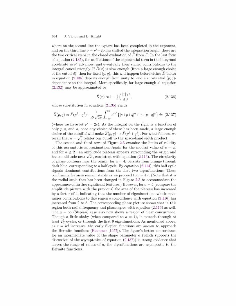
where on the second line the square has been completed in the exponent,and on the third line ν = ν′+2p has shifted the integration origin; these arethe two critical steps in the closed evaluation of F from F . In the last formof equation (2.135), the oscillations of the exponential term in the integrandaccelerate as ν′ advances, and eventually their signed contributions to theintegral cancel strongly. If D(x) is slow enough (from a large enough choiceof the cutoff d), then for fixed (p, q), this will happen before either D factorin equation (2.135) departs enough from unity to lend a substantial (p, q)-dependence to the integral. More specifically, for large enough d, equation(2.132) may be approximated by

D(x) ≈ 1− 12

( |x|d

)a

, (2.136)

whose substitution in equation (2.135) yields

Z(p, q) ≈ F (p2+q2)− 1da√

2π

∫ ∞

−∞eis2{

|s+p+q|a+|s+p−q|a}ds (2.137)

(where we have let ν′ = 2s). As the integral on the right is a function ofonly p, q, and a, once any choice of these has been made, a large enoughchoice of the cutoff d will make Z(p, q) → F (p2 + q2). For what follows, werecall that d =

√c relates our cutoff to the space-bandwidth product.

The second and third rows of Figure 2.5 examine the limits of validityof this asymptotic approximation. Again for the modest value of c = π,and for a ≥ 2 , an amplitude plateau appears surrounding the origin andhas an altitude near

√2 , consistent with equation (2.116). The circularity

of phase contours near the origin, for a = 4, persists from orange throughdark blue, corresponding to a half cycle. By equation (2.114), this half cyclesignals dominant contributions from the first two eigenfunctions. Theseconfirming features remain stable as we proceed to c = 4π. (Note that it isthe radial scale that has been changed in Figure 2.5 to accommodate theappearance of further significant features.) However, for a = 4 (compare theamplitude picture with the previous) the area of the plateau has increasedby a factor of 4, indicating that the number of eigenfunctions which makemajor contributions to this region’s concordance with equation (2.116) hasincreased from 2 to 8. The corresponding phase picture shows that in thisregion both radial frequency and phase agree with equation (2.116) as well.The a = ∞ (Slepian) case also now shows a region of clear concurrence.Though a little shaky (when compared to a = 4), it extends through atleast 2 1

4 cycles, or through the first 9 eigenfunctions. As mentioned above,as c = bd increases, the early Slepian functions are known to approachthe Hermite functions (Flammer [1957]). The figure’s better concordancefor an intermediate value of the shape parameter a (which supports thediscussion of the asymptotics of equation (2.137)) is strong evidence thatacross the range of values of a, the eigenfunctions are asymptotic to theHermite functions.


(A)

Figure 5A

p

a =1 a =2 a =4 a = •

q

K~

Z~

Z~

arg

(a)

(B)

p

a =1 a =2 a =4 a = •

q

K~

Z~

Z~

arg

Figure 5b(b)

(C)

Figure 5C

p

a =1 a =2 a =4 a = •

q

K~

Z~

Z~

arg

(c)

Figure 2.5. Comparison of the Wigner transforms K(p, q) and Z(p, q) for thevalues of the shape parameter a and scale parameters b and d of Figure 2.4. Ineach panel, first row: K(p, q); second row: amplitude of Z(p, q); third row: phase

of Z(p, q). A common color scale for amplitude, running from blue to deep red, isused for the first two rows. Color scale for third row: red corresponds positive real,yellow to positive imaginary, green to negative real, blue to negative imaginary.


Return to the general self-adjoint operator (Dd)12Bb(Dd)

12 = DdBdDd,

where Dd and Bb are defined by the one-dimensional analogs of equations(2.1) and (2.2), respectively. To show that the above considerations applyeven if b 6= d, we reconsider the scaled Fourier transform operator Fγ , asdefined by equation (2.113). It follows from the definitions of B and D that

Bb = PFγDbγFγ = (Fγ)−1DbγFγ , (2.138)

generalizing equation (2.119). Hence, if we choose

γ =d

b, (2.139)

we findDdBdDd = DdPFγDdFγDd . (2.140)

Symmetry considerations again require that any eigenfunction ψ ofDdBbDd is either even- or odd-symmetric. Thus, if ψ is an eigenfunctionof DdBbDd

DdBbDdψ = PZ2ψ, (2.141)

where we have definedZ = DdFγDd , (2.142)

generalizing equation (2.127).We now proceed to find the Wigner transform Z of Z, where

Z{x, x′} =1√2πγ

Dd(x)Dd(x′)e−ixx′/γ . (2.143)

The substitutions ν = x − x′ and q = 12 (x + x′), followed by Fourier

transformation with respect to ν, leads to an expression for the Wignertransform of Z,

Z(p, q) =1√2πγ

∫ ∞

−∞Dd

(q +

12ν

)Dd

(q − 1

2ν)e−i(q2− 1

4 ν2)/γe−iνp dν ,

(2.144)which is rearranged to

Z(p, q) =1√2πγ

e−i(q2/γ+p2γ)

∫ ∞

−∞Dd

(q + 1

2ν)Dd

(q − 1

2ν)ei(ν−2pγ)2/4γ dν ,

(2.145)generalizing equation (2.135). For a = 2, the integral can be performedexactly:

Z(p, q) =

√2

1bd − i

exp(− q

2

d2(1 + ibd)− p2d2

1− ibd

). (2.146)


In the limit of a → ∞, the second derivatives of the integral (2.145) atthe origin behave similarly to those of K: ∂2Z

∂p2 is analytic, ∂2Z∂p∂q is zero,

and ∂2Z∂q2 is undefined. Thus, a Gaussian approximation for Z is no more

justified than for K. However, as in the special case of b = d consideredabove, the integral (2.145) can be approximated directly for the generala > 2, if, within the vicinity of ν = 2pγ , the functions Dd are slowlyvarying. This condition translates to∣∣q ± pγ

∣∣ � 21/a d . (2.147)

(The factor 21/a originates from the square root of the operator Dd.) Thisalso takes the more symmetric form∣∣ q

√γ± p

√γ∣∣ � 21/a

√bd . (2.148)

The above condition is satisfied if both |q| � d and |p| � b, that is,within the band- and space-limits specified byD and B, respectively. In thisregime, the dominant contribution to the integral (2.145) can be obtainedby replacing D with its peak value, 1. This leads to

Z(p, q) ≈ (1 + i)e−i(q2/γ+p2γ) , (2.149)

generalizing the approximation of equation (2.135) by equation (2.116).The approximate Wigner transform, equation (2.149), has contour lines

that are ellipses parallel to the (q, p) coordinate axes. Moreover (similarto equation (2.89) above), these contour lines can be made circular by thesymplectic transformation q′ = q√

γ , p′ = p

√γ. Z is not Hermitian, but it

is normal — that is, it commutes with its adjoint. As we have seen above,this suffices for the analysis of Knight and Sirovich [1986] to be applicable.In particular, we can conclude that within the regime specified by equation(2.148), the eigenfunctions of Z, and hence of DdBdDd,are approximatedby the Hermite functions.

Thus, we have generalized the asymptotic relationship of Flammer [1957]between the Hermite functions and the Slepian functions (which extremizespace and band limits in the sense of a = ∞) to functions which extremizespace and band limits for any choice of the shape parameter a in (0,∞).As the next section shows, certain features of our analysis apply even moregenerally, and in particular do not require specification of the shape for thespace or band-limiter.

A Perturbation Analysis

For the particular case of a = 2 (the Gaussian case), we have an exactsolution for the eigenvalues and eigenfunctions of Z. We have seen thatthe spectrum separates naturally into four subsets which respectively are


given by {1,−i,−1, i}, each multiplied by a set of positive numbers lessthan unity and descending to zero. Since K = PZ2 (equations (2.126) and(2.127)), this characterization of the eigenfunctions and eigenvalues of Zdetermines the behavior of the eigenfunctions and eigenvalues of K.

Here we use a perturbation argument to show that this behavior isgeneric. In contrast to the previous arguments, this aspect of the analysisis rather general, and does not depend on the precise form of the space-limiting function D or the band-limiting function B, provided that theyare even-symmetric and Fourier transforms of each other.

Under these conditions, it suffices to consider the integral kernel of equa-tion (2.130), Z = DFD, which can be recast in the more general form

Z{x, x′} =1√2π

e−Γ(x,t)e−ixx′e−Γ(x′,t) , (2.150)

where t is a parameter that smoothly specifies the shape of the space-limiting function D (or D), and Γ is real. In particular, we can specify thatt = 0 corresponds to the Gaussian (“soft”) case, and t = 1 correspondsto the Slepian (“hard”) case, but for the present argument, the shapesspecified by intermediate values of t need not be specified. Several choicesof the parameterization by t are of interest, which includes allowing t tocontrol a or d, the parameters that already appear in the definition (2.85)of D. Our goal is to determine how the eigenvalues ζn of equation (2.133)depend on t.

Since the eigenvectors ϕn may be chosen to be orthonormal, it followsfrom the eigenvalue equation (2.133) that

ζn = (ϕn , Zϕn) . (2.151)

Consequently,

dζndt

= −(ϕn , (ΓtZ + ZΓt)ϕn

)= −2ζn(ϕn ,Γtϕn) , (2.152)

where Γt ≡ ∂∂tΓ(x, t). (We have used (ϕn ,

∂∂tϕn) = 0 which follows from

orthonormality.) The differential equation (2.152) is readily integrated toobtain an expression for the eigenvalues ζn:

ζn(t) = ζn(0)e−2∫ t0 cn(t′) dt′ , (2.153)

wherecn(t) =

(ϕn(t) ,Γtϕn(t)

). (2.154)

Thus, as the kernel Z of equations (2.130) and (2.150) varies parametricallywith t, its eigenvalues vary according to equation (2.153).

The integral in equation (2.153) is real. This means that the eigenvaluesζn(t) necessarily have the same phase as ζn(0). By choosing D = 1 at t = 0,(so Z = F , the infinite space-bandwidth limit) we can thus infer from


equation (2.114) that the phase of ζn(t) is equal to − 12nπ for the general

Z. Finally, we note that if the parametric dependence of γ on t is monotoneincreasing (corresponding, for example, to space-limiting functions D thatare successively narrower), then equation (2.153) implies that as t increases,each of the eigenvalues ζn(t) shrinks monotonically towards zero along acardinal axis.

2.8 The Non-Gaussian Case: Two Dimensions

The above analysis of the operator Z can be applied directly to the two-

dimensional operators D12BD

12 . This implies a corresponding asymptotic

relationship between the eigenfunctions for the general operators D12BD

12

(or BD) and those for the Gaussian case.In two dimensions, the operators B,D, and their products do not sep-

arate in Cartesian coordinates for a 6= 2 . However, they do have exactrotational symmetry (including a 6= 2). This symmetry, and the separationinto polar coordinates that it implies, means that one can find a completeset of eigenfunctions, all of which have an angular dependence of the formeiµθ for some integer µ. Conversely, for each integer µ, we anticipate a dis-crete set of eigenfunctions ψµ,ν(R, θ) = eiµθζµ,ν(R), where ν counts thenumber of zero-crossings in the radial dependence ζµ,ν(R). In the Gaussiancase, the corresponding eigenvalue λµ,ν depends only on 2ν + |µ|. This de-generacy is a consequence of the dual separation into polar and Cartesiancoordinates, equation (2.50).

In sum, the above analysis shows that for the general shape parametera, the two-dimensional functions are also parameterized by a non-negativeinteger ν that counts the number of zero-crossings along a radius, anda second integer µ (which may be negative) that describes the angulardependence. In view of the asymptotic relationship of the general one-dimensional functions and the Hermite functions, we anticipate that theeigenvalue associated with ν and µ asymptotically depends only on 2ν+|µ|.

2.9 V4 Receptive Fields

One of our motivations for studying functions that are simultaneouslyspace- and band-limited is to gain some insight into neural processing ofvisual images beyond primary visual cortex (V1), and especially in V4. Theextrastriate area V4 appears to be an important area for the analysis ofshape Merigan [1996]. The behavior of neurons in V4 differs dramaticallyfrom those of its inputs, V1 and V2. Neurons in V1 and V2 usually canbe characterized as having a single preferred orientation, and respond wellto a grating of an appropriately chosen spatial frequency, especially if thegrating is limited in spatial extent. Known differences between V1 and V2neurons are relatively subtle (Levitt, Kiper, and Movshon [1994]), and con-


sist mainly of differences in overall receptive field size, contrast sensitivity,and the prominence of responses to illusory contours (Grosof, Shapley, andHawken [1993]; von der Heydt, Peterhans, and Baumgartner [1984]). Incontrast, V4 neurons do not have a clear orientation preference, are oftendifficult to stimulate with gratings, and typically require complex stimulifor strong responses (Kobatake and Tanaka [1994]).

Consequently, systematic study of the spatial structure of the receptivefields of V4 neurons has been difficult. One of the few successful examples isthe provocative study by Gallant, Braun, and Van Essen [1993] and Gallant,Connor, Rakshit, Lewis, and Van Essen [1996]. V4 neurons were stimulatedwith patches of standard (“Cartesian”) gratings, and also patches of “po-lar” gratings and patches of “hyperbolic” gratings (Figure 2.6). The polargratings include target- and pinwheel-like stimuli; the hyperbolic gratingsconsist of alternating bands of light and dark that form rectangular hyper-bolae with shared asymptotes. The main finding was that many V4 neuronswere well-stimulated by particular examples of non-Cartesian stimuli. Al-though some neurons responded substantially better to members of oneclass of gratings than to the other two, most neurons had broad tuningsacross these classes (that is, they responded almost as well to some stimuliof the non-preferred class as to the best stimulus). Moreover, the typicalneuron responded relatively poorly to most stimuli, even within its pre-ferred class.

To determine whether this kind of behavior is expected from neuronsthat filter the image in a manner that is both space and band-limited,we performed a crude simulation. Receptive field profiles were constructedfrom the two-dimensional eigenfunctions for BD (Gaussian case), for val-ues of the circular symmetry index µ ∈ {0, 1, 2, 4} and for a range of radialnodes ν ∈ {0, 1, 2, 3}. We chose the space-bandwidth product c = bd = 4.The resulting profiles are shown in Figure 2.7. Raw “responses” were calcu-lated simply by evaluating the inner product of each stimulus in Figure 2.6with the receptive field profile. (The stimulus was considered to have a realpart, as specified by Gallant, Braun, and Van Essen [1993]; Gallant, Con-nor, Rakshit, Lewis, and Van Essen [1996], and a corresponding imaginarypart, obtained by replacing cosines by sines. Thus, this highly schematizedmodel essentially posits a quadrature pair operation that removes the ef-fect of the spatial “phase” of the Cartesian or non-Cartesian grating.) Foreach receptive field profile, the raw responses were then normalized by thelargest quadrature pair response encountered to any of the stimuli.

A histogram of the normalized responses obtained for each receptive fieldprofile is shown in Figure 2.8. Several features are immediately apparent.As in the data of Gallant, Braun, and Van Essen [1993]; Gallant, Con-nor, Rakshit, Lewis, and Van Essen [1996], most receptive fields respondedpoorly to most stimuli – as evidenced by the large peaks in most of the his-tograms at a response size of 0. The receptive fields corresponding to µ = 1responded almost exclusively to Cartesian gratings. This is a consequence


cartesian

polar

hyperbolic

Figure 2.6. Some of the stimuli used by Gallant, Braun, and Van Essen [1993];Gallant, Connor, Rakshit, Lewis, and Van Essen [1996]. The full stimulus setincluded three other spatial frequencies for each stimulus class, and also counter-clockwise variants of the “polar” stimuli — for a total of 30 Cartesian gratings,45 polar gratings, and 20 hyperbolic gratings.

µ=2

µ=1

µ=0

µ=4

ν=0 ν=1 ν=2 ν=3

Figure 2.7. Receptive field sensitivity profiles (real parts) used for the simulation.All profiles had a space bandwidth product c = 4. The size of the disk correspondsto the region of space that covered the test stimuli, taken from Gallant, Braun,and Van Essen [1993]; Gallant, Connor, Rakshit, Lewis, and Van Essen [1996](see Figure 2.6).


of the symmetry of these receptive fields. Among the other profiles, many(µ = 4) had optimal responses to polar gratings, and one (µ = 0, ν = 1)had an optimal response to a hyperbolic grating. The profiles correspond-ing to µ = 2 tended to have large responses to some Cartesian and somepolar gratings, while the profiles corresponding to µ = 4 tended to havelargest responses to polar gratings, with next-largest responses to hyper-bolic gratings.

3 Discussion

This paper describes two-dimensional profiles that are simultaneously lim-ited in spatial extent and in bandwidth. The main motivation is to general-ize ideas that have benefited the study of visual processing in primary visualcortex, V1. As outlined above, V1 neurons, to a first approximation, are of-ten thought of as one-dimensional spatial analyzers. They generally have awell-defined orientation preference, and typically they can be characterizedby their responses to windowed gratings. However, there are indicationsthat visual processing by individual neurons, even in V1, is not restrictedto a single orientation (Purpura, Victor, and Katz [1994]). Moreover, cer-tain aspects of early visual processing (whose physiologic locus is uncer-tain) make explicit use of two-dimensional information, such as extractionof T-junctions (Rubin [2001]), curvature (Wolfe, Yee, and Friedman-Hill[1992]), texture (Victor and Brodie [1978]) and shape (Wilkinson, Wilson,and Habak [1998]). Finally, neurons beyond V1 and V2 are generally notwell-stimulated by standard gratings or other simple stimuli, which makesquantitative study of such neurons a challenge (Gallant, Braun, and VanEssen [1993]; Gallant, Connor, Rakshit, Lewis, and Van Essen [1996]; Ko-batake and Tanaka [1994]; Tanaka, Saito, Fukada, and Moriya [1991]).

Our notion of simultaneous confinement in space and spatial frequencyis distinct from the notion in Daugman [1985] of minimizing uncertainty intwo important respects. First, (see equations (2.8) and (2.9) and surround-ing material), our notion seeks profiles that are least altered by applicationof linear operators that truncate influences that are non-local in space (D)or spatial frequency (B). In contrast, Daugman [1985]’s notion directlyadopts Gabor [1946]’s idea of seeking profiles that minimize joint spreadin space and spatial frequency, as quantified by a Heisenberg uncertaintyproduct. Secondly, our approach considers the profiles themselves as thesubject for extremization. Though the profiles naturally group into realand imaginary pairs (lower portions of Figure 2.2 and Figure 2.3), theyare intrinsically real, and their positive and negative lobes are intrinsic totheir extremal properties. Daugman’s approach focuses on the magnitude-squared of the profiles (Stork and Wilson [1990]); the positive and negativelobes of the derived profiles only arise because of phase factors eiωx that


µ=2

µ=1

µ=0

µ=4

ν=0

ν=1

ν=2

ν=3

Figure 2.8. Summary of responses of the receptive fields of Figure 2.7 to Carte-sian, polar, and hyperbolic gratings. The three histograms in each frame representresponses to the three classes of grating stimuli: Cartesian gratings (30 total),dark; polar gratings (45 total), gray; hyperbolic gratings (24 total), light. Thehorizontal axis represents response size, normalized by the largest quadrature pairresponse across all three classes. The height of each histogram bar represents thenumber of stimuli that elicited a response of each (normalized) size.


are irrelevant to the extremal properties.Interestingly, applying the Gabor/Daugman approach to real-valued func-

tions (Gabor [1946]; Stork and Wilson [1990]) identifies one-dimensionalHermite functions as playing an extremal role, but this role proves to bethat of maximizing uncertainty within the space of polynomials multipliedby Gaussians, rather than minimizing it (Klein and Beutter [1992]).

The families of functions presented here have attributes that recommendthem as a natural extension of windowed gratings. Since each family formsa complete orthogonal set, its members can serve as a basis for charac-terization of the quasilinear aspects of a neuron’s response, either as in-dividual stimuli presented in discrete trials or as members of a rapidly-presented stimulus sequence (Ringach, Sapiro, and Shapley [1997]). Moreimportantly, these functions can serve as a common stimulus set to deter-mine how spatial processing evolves from V1 to V4. From the point of viewof V1, these families of functions contain elements (those with one index 0in Cartesian separation) that are very similar to Gabor patches (Swanson,Wilson, and Giese [1984]). From the point of view of V4, the families (inpolar separation) contain elements that resemble the non-Cartesian grat-ings used by Gallant and co-workers. With these stimuli, hypotheses for theorganization and relationship of V1 and V4 receptive fields can readily betested. For example, if indeed V1 neurons are one-dimensional analyzers,there should be little response to functions which, in the Cartesian sepa-ration ψnx

(x)ψny(y), have both indices nx and ny nonzero. On the other

hand, if V1 neurons only appear to be one-dimensional analyzers becausethey have a limited space-bandwidth product, then neurons that respondto an intrinsically two-dimensional function such as ψ1(x)ψ1(y) should beabout as common as neurons that respond to a one-dimensional multilobedfunction, such as ψ2(x)ψ0(y), of equal eigenvalue. The hypothesis that pro-cessing in V4 is intrinsically two-dimensional, rather than just characterizedby an increased space-bandwidth product, makes the converse prediction.

As noted above, the “Gabor” profiles of typical neurons in V1 have onlyone or two major lobes, and equally well might be replaced by functionssuch as ψ1(x)ψ0(y) and ψ2(x)ψ0(y), with an appropriate choice of axes.Wilson [1999], drawing on anatomical work by Schoups, Tootell, and Orban[1995], has suggested that V4 neurons obtain their properties by pooling ofV1 responses across multiple orientations, and that circularly symmetric V4receptive fields might result from uniform pooling of one-dimensional pro-files in V1. Appropriately weighted combinations of profiles at orthogonalorientations also can lead to receptive field sensitivity profiles with n-foldrotational symmetry, for arbitrary n, as seen from the relationship betweenthe Cartesian and polar separations described above. Neurons with prefer-ences for n-fold rotational symmetry have been encountered in extrastriatecortices (Tanaka, Saito, Fukada, and Moriya [1991]). It is interesting (andalso highly speculative) to note that the relationship between the polarseparation and the Cartesian separation provides an economical way to


construct receptive fields of arbitrary rotational symmetry.Our crude analysis (Figure 2.8) of simulated neurons based on the eigen-

functions in polar separation indicates that these receptive field profilesindeed can be tuned for Cartesian and non-Cartesian gratings, as Gallant,Braun, and Van Essen [1993]; Gallant, Connor, Rakshit, Lewis, and VanEssen [1996] found for real V4 neurons. Given the highly schematized andsimple nature of our simulation, a detailed correspondence with physiol-ogy would be unexpected. Indeed, only certain aspects of Gallant et al.’sresults are accounted for by this scheme. Gallant et al. found tuning tohyperbolic gratings that was more prominent than our simulations sug-gest. They also found that responses were relatively insensitive to transla-tions of the stimulus. This suggests that the very simple scheme we usedhere (inner product followed by a quadrature-pair calculation) needs tobe augmented by additional stages of processing, perhaps in the form ofreceptive field subunits. More detailed modeling in this direction requiresadditional physiologic data, and is beyond the scope of this work. However,it is hoped that the considerations presented here will serve as a basis fora sound theoretically-motivated experimental approach to understandingvisual processing beyond the earliest cortical stages.

4 Appendix

Normalization of the Eigenfunctions in the Gaussian Case. Thenormalization of the eigenfunctions (2.29) requires integrals similar to equa-tion (2.58), but with respect to Gaussians of variance other than unity.The generating-function strategy used for the evaluation of the integrals ofequation (2.58) readily extends to this situation. First, consider

12πV

∫∫ ∞∑0

zktl qk,l(x, y)k! l!

z′k′t′l

′qk′,l′(x, y)k′! l′!

exp[− 1

2V(x2 + y2)

]dx dy

=1

2πV

∫∫Q(z, t)Q(x′, t′) exp

[− 1

2V(x2 + y2)

]dx dy (4.1)

in which the sum on the left-hand side is over all values of k, l, k′ and l′.Proceeding in the same manner as with equation (2.58), we find

12πV

∫∫ ∞∑0

zktlqk,l(x, y)k! l!

z′k′t′l

′qk′,l′(x, y)k′! l′!

exp[ 12V

(x2 + y2)]dx dy

= exp[2V (zz′ + tt′)

]exp

[2(V − 1)(zt+ z′t′) .

](4.2)

Because of the polar symmetry, terms for which k−l 6= k′−l′ are necessarily0. Extracting and equating terms corresponding to zµ+νtν(z′)µ+ω(t′)ω leads


to

12πV

∫∫qµ+ν,ν(x, y) qµ+ω,ω(x, y) exp

[− 1

2V(x2 + y2)

]dx dy

= (µ+ ν)!ν!(µ+ ω)!ω!∑

α,β,γ,δ

2α+β+γ+δ(V − 1)α+βV γ+δ

α!β! γ! δ!, (4.3)

where the sum is over all indices α, β, γ and δ satisfying

α+ γ = µ+ ν

α+ δ = ν

β + γ = µ+ ω

β + δ = ω . (4.4)

Equation (4.3) leads to

12πV

∫∫qµ+ν,ν(x, y) qµ+ω,ω(x, y) exp

[− 1

2V(x2 + y2)

]dx dy

= 2µ+ν+ω(µ+ ν)! ν! (µ+ ω)!ω!min(ν,ω)∑

s

(V − 1)ν+ω−2s V µ+2s

(ν − s)! (ω − s)! s! (µ+ s)!.

(4.5)

The general result (4.5) can also be recast as

1V

∫ ∞

0

Pµ,ν(R2)Pµ,ω(R2)R2µ+1 exp(−R

2

2V

)dR

= 2µ+ν+ω(µ+ ν)! ν! (µ+ ω)!ω!min(ν,ω)∑

s

(V − 1)ν+ω−2sV µ+2s

(ν − s)! (ω − s)! s! (µ+ s)!.

(4.6)

To see the relationship to the case V = 1 of equation (2.58), note that theonly nonzero contributions to the sum in equation (4.3) are for α = β = 0which forces γ = µ + ν = µ + ω and δ = ν = ω. In equations (4.5) and(4.6), this corresponds to the sole term s = ν = ω, which establishes thereduction to equation (2.60) with κ = µ + ν and l = ν and to equation(2.62).

Modest Non-Orthogonality After Shifts. The extent to which shift-ing a function spoils the orthogonality can be captured by consideringthe Hermite-function limit (large c) of the one-dimensional eigenfunctions.These eigenfunctions (see equations (2.21) and (2.27)) are given by

ϕn(x) = hn(kx) exp(− 1

4k2x2

), (4.7)


from which it follows that∞∑

n=0

zn

n!ϕn(x) = exp

(− 1

4k2x2 + kxz − 1

2z2). (4.8)

To determine the non-orthogonality of themth and nth eigenfunctions afterpositional shifts s, define

am,n(x) =k√2π

∫ ∞

−∞ϕm(x− s)ϕn(x+ s) dx . (4.9)

Consider a generating function defined by

A(s, y, z) =∞∑

m=0

∞∑n=0

ym

m!zn

n!am,n(s) . (4.10)

From the generating function (4.8) for ϕ, it follows that

A(s, y, z) =k√2π

∫ ∞

−∞exp

(− 1

4k2(x− s)2 + k(x− s)y − 1

2y2)

exp(− 1

4k2(x+ s)2 + k(x+ s)z − 1

2z2)dx , (4.11)

and hence,

A(s, y, z) =k√2π

exp(− 1

2k2s2 + ks(−y + z)

)∫ ∞

−∞exp

(− 1

2k2x2 + kx(y + z)− 1

2y2 + z2

)dx

= exp(− 1

2k2s2 + ks(−y + z) + yz

). (4.12)

Equating coefficients of terms ymzn in equations (4.10) and (4.12) yields:

am,n(s) =min(m,n)∑

j=0

(−1)m−jj!(m

j

)(n

j

)(ks)m+n−2j exp

(− 1

2k2s2

).

(4.13)Note that when s = 0, the only nonzero term on the right-hand side ofequation (4.13) has m+ n− 2j = 0, which can only occur if m = n (thus,recovering orthogonality when there is no shift). For nonzero s, the valuesof am,n(s) are controlled by the Gaussian envelope.

Acknowledgments: This work was supported by NIH NEI EY9314 andDARPA MDA972-01-1-0028. The authors thank Partha Mitra and LarrySirovich for several helpful discussions, Stan Klein and Hugh Wilson forinsightful comments on the manuscript, and Adam Kahn for programmingassistance.


References

Abramowitz, M. and I. A. Stegun [1964], Handbook of Mathematical Functions.National Bureau of Standards. Reprinted by Dover, New York, 1970.

Atick, J. and A. Redlich [1990], Towards a theory of early visual processing,Neural Comput. 2, 308–320.

Daugman, J. G. [1985], Uncertainty relation for resolution in space, spatial fre-quency, and orientation optimized by two-dimensional visual cortical filters, JOpt Soc Am [A]. 2, 1160–9.

Erdelyi, A. [1955], Higher Transcendental Functions. Bateman ManuscriptProject, Vol. II. New York: McGraw-Hill.

Field, D. J. (1994), What is the goal of sensory coding? Neural Comput. 6: 559–601.

Flammer, C. [1957], Spheroidal Wave Functions. Stanford: Stanford UniversityPress.

Gabor, D. [1946], Theory of communication, J. Inst. Elect. Eng. 93, 429–457.

Gallant, J. L., J. Braun, and D. C. Van Essen [1993], Selectivity for polar, hyper-bolic, and Cartesian gratings in macaque visual cortex, Science, 259, 100–3.

Gallant, J. L., C. E. Connor, S. Rakshit, J. W. Lewis, and D. C. Van Essen[1996], Neural responses to polar, hyperbolic, and Cartesian gratings in areaV4 of the macaque monkey, J Neurophysiol. 76: 2718–39.

Grosof, D. H., R. M. Shapley, and M. J. Hawken [1993], Macaque V1 neuronscan signal ‘illusory’ contours, Nature. 365, 550–2.

Halmos, P. [1942], Finite Dimensional Vector Spaces. Princeton: Princeton Uni-versity Press.

Jones, J. P. and L. A. Palmer [1987], An evaluation of the two-dimensional Gaborfilter model of simple receptive fields in cat striate cortex, J Neurophysiol. 58,1233–58.

Klein, S. A. and B. Beutter [1992], Minimizing and maximizing the joint space-spatial frequency uncertainty of Gabor-like functions: comment, J. Opt. Soc.Am. A 9, 337–40.

Knight, B. W. and L. Sirovich [1982], The Wigner transform and some exactproperties of linear operators, SIAM J. Appl. Math. 42, 378–389.

Knight, B. W. and L. Sirovich [1986], The eigenfunction problem in higher di-mensions: Exact results, Proc. Natl. Acad. Sci. USA 83, 527–530.

Kobatake, E. and K. Tanaka, [1994], Neuronal selectivities to complex objectfeatures in the ventral visual pathway of the macaque cerebral cortex, J Neu-rophysiol. 71, 856–67.

Laughlin, S. B., R. R. de Ruyter van Steveninck, and J. C. Anderson [1998], Themetabolic cost of neural information, Nat Neurosci. 1, 36–41.

Levitt, J. B., D. C. Kiper, and J. A. Movshon[1994], Receptive fields and func-tional architecture of macaque V2, J Neurophysiol. 71, 2517–42.

Marcelja, S. [1980], Mathematical description of the responses of simple corticalcells, J Opt Soc Am. 70, 1297–1300.


Merigan, W. H. [1996], Basic visual capacities and shape discrimination afterlesions of extrastriate area V4 in macaques, Vis Neurosci. 13, 51–60.

Percival, D. and A. Walden [1993], Spectral Analysis for Physical Applications:Multitaper and Conventional Univariate Techniques. Cambridge: CambridgeUniversity Press.

Purpura, K. P., J. D. Victor, and E. Katz [1994], Striate cortex extracts higher-order spatial correlations from visual textures, Proc Natl Acad Sci U S A. 91,8482–6.

Ringach, D. L., G. Sapiro, and R. Shapley [1997], A subspace reverse-correlationtechnique for the study of visual neurons, Vision Res. 37, 2455–2464.

Rota, G.-C. and B. D. Taylor [1994] The classical umbral calculus, SIAM J. Math.Anal. 25, 694–711.

Rubin, N. [2001], The role of junctions in surface completion and contour match-ing, Perception 30, 339–366

Schoups, A. A., R. B. Tootell, W. Vanduffel, and G. A. Orban [1995], Use of thedouble-label deoxyglucose approach to map the orientation columnar systembeyond area V1 and V2 in the macaque, and its plasticity, Soc. Neurosci. Abstr.21, 18.

Sirovich, L. and B. W. Knight [1981], On the eigentheory of operators whichexhibit a slow variation, Quart. Appl. Math. 38, 469–488.

Sirovich, L. and B. W. Knight [1982], Contributions to the eigenvalue problemfor slowly varying operators, SIAM J. Appl. Math. 42, 356–377.

Sirovich, L. and B. W. Knight [1985], The eigenfunction problem in higher di-mensions: Asymptotic Theory, Proc. Natl. Acad. Sci. USA. 82, 8275–8278.

Slepian, D. and H. O. Pollack [1961], Prolate spheroidal wave functions, Fourieranalysis and uncertainty I. Bell Syst. Tech. J. 40, 43–64.

Slepian, D. [1964], Prolate spheroidal wave functions, Fourier analysis and un-certainty IV: Extensions to many dimensions; generalized prolate spheroidalfunctions, Bell Syst. Tech. J. 43, 3009–3057.

Stork, D. G. and H. R. Wilson [1990], Do Gabor functions provide appropriatedescriptions of visual cortical receptive fields?, J. Opt. Soc. Am. A 7, 1362–73.

Swanson, W. H., H. R. Wilson, and S. C. Giese [1984], Contrast matching datapredicted from contrast increment thresholds, Vision Res. 24, 63–75.

Tanaka, K., H. Saito, Y. Fukada, and M. Moriya [1991], Coding visual images ofobjects in the inferotemporal cortex of the macaque monkey, J Neurophysiol.66, 170–89.

Victor, J. D. and S. Brodie [1978], Discriminable textures with identical Buffonneedle statistics, Biological Cybernetics 31, 231–234.

Vilenkin, N. J. [1968], Special Functions and the Theory of Group Representa-tions. American Mathematical Society.

von der Heydt, R., E. Peterhans, and G. Baumgartner [1984], Illusory contoursand cortical neuron responses, Science 224, 1260–2.

Wilkinson, F., H. R. Wilson, and C. Habak [1998], Detection and recognition ofradial frequency patterns, Vision Res. 38, 3555–68.


Wilson, H. R. [1999] Non-Fourier cortical processes in texture, form, and motionperception. In Cerebral Cortex, vol. 13, pages 445–477. ed: Ulinski et al. KluwerAcademic, New York.

Wilson, H. R. and F. Wilkinson [1998], Detection of global structure in Glasspatterns: implications for form vision, Vision Res. 38, 2933–47.

Wolfe, J. M., A. Yee, and S. R. Friedman-Hill, [1992], Curvature is a basic featurefor visual search tasks, Perception 21, 465–80.

Xu, Y., S. Haykin, and R. J. Racine [1999], Multiple window time-frequencydistribution and coherence of EEG using Slepian sequences and Hermite func-tions, IEEE Trans. Biomed. Engrg. 46, 861–866.

perspectives and problems in nonlinear sciencejdvicto/pdfs/vikn03.pdf · perspectives and problems...

Documents