VILNIUS UNIVERSITY

Andrej Kisel

PERSON IDENTIFICATION BY FINGERPRINTS AND VOICE

Doctoral Dissertation

Physical sciences, informatics (09 P)

Vilnius, 2010

2

The work was performed in 2005 – 2010 at Vilnius University

Supervisor:

Doc. Dr. Algirdas Bastys (Vilnius University, Physical sciences, informatics – 09 P)

1

Table of Contents

Table of Contents 1

Abstract 4

1 Introduction 4

1.1 Research Area............................................................................................. 4

1.2 Fingerprint biometrics ................................................................................ 5

1.2.1 Fingerprint structure ........................................................................... 5

1.2.2 Fingerprint acquisition ........................................................................ 6

1.2.3 Fingerprint features ............................................................................. 7

1.2.4 Fingerprint matching ........................................................................... 9

1.2.5 Fingerprint classification ..................................................................... 10

1.2.6 Extraction of fingerprint features ........................................................ 11

1.2.7 Fingerprint recognition performance evaluation ............................... 12

1.3 Voice Biometrics ......................................................................................... 14

1.3.1 Speaker identification and verification tasks ...................................... 14

1.3.2 Text-dependent and text-independent speaker recognition ............. 16

1.3.3 Speaker modeling techniques ............................................................. 18

1.3.3.1 Speech signal processing, features ............................................... 18

1.3.3.2 Mel Cepstrum ............................................................................... 19

1.3.3.3 Linear prediction ........................................................................... 20

1.3.3.4 LPC-based cepstral parameters .................................................... 22

1.3.3.5 Additional transformations .......................................................... 23

1.3.4 Models of Speakers and their matching ............................................. 24

1.3.4.1 Template Models .......................................................................... 25

1.3.4.2 Dynamic Time Warping ................................................................ 25

1.3.4.3 Vector Quantization approach ..................................................... 27

1.3.4.4 Nearest Neighbors method .......................................................... 28

1.3.4.5 Stochastic models ......................................................................... 28

1.3.4.6 Gaussian Mixture Model .............................................................. 30

1.3.5 Speaker recognition by Lithuanian authors ........................................ 32

2

1.4 Problem Relevance ..................................................................................... 33

1.5 Research Objects ........................................................................................ 34

1.6 The Objectives and Tasks of the Research ................................................. 34

1.7 Scientific Novelty ........................................................................................ 35

1.8 Practical Importance of the Work .............................................................. 35

1.9 Approval of Research Results ..................................................................... 36

1.10 Defended propositions ............................................................................... 36

1.11 Publications ................................................................................................ 37

1.12 Outline of the Thesis .................................................................................. 37

2 Fingerprint image synthesis 38

2.1 Introduction ................................................................................................ 38

2.2 SFINGE ........................................................................................................ 40

2.2.1 Fingerprint form .................................................................................. 40

2.2.2 Fingerprint type and orientation map ................................................. 41

2.2.3 Ridge density map generation ............................................................ 42

2.2.4 Ridge generation ................................................................................. 42

2.2.5 Analysis ................................................................................................ 44

2.3 Modified SFINGE Method .......................................................................... 44

2.4 Correlation of synthetic fingerprints and real fingerprints ....................... 47

2.5 Extraction algorithm performance evaluation .......................................... 49

2.6 Experiments ................................................................................................ 51

2.7 Summary and Conclusions of the Chapter ................................................. 55

3 Fingerprint matching 56

3.1 Introduction ................................................................................................ 56

3.2 Fingerprint Matching Without Global Alignment ...................................... 59

3.3 Local Matching ........................................................................................... 59

3.3.1 Local Structure ..................................................................................... 59

3.3.1.1 Similarity Score ............................................................................. 60

3.3.2 Correspondence Set Construction ...................................................... 61

3.4 Validation ................................................................................................... 62

3.4.1.1 Similarity Score ............................................................................. 64

3.5 Final Similarity Score .................................................................................. 64

3.6 Evaluation of threshold parameters .......................................................... 65

3

3.6.1 Threshold Parameters in Local Structures .......................................... 65

3.6.2 Threshold Parameters in Similarity Functions .................................... 66

3.7 Performance Evaluation ............................................................................. 67

3.8 Results ........................................................................................................ 68

3.9 Summary and Conclusions of the Chapter ................................................. 70

4 Speaker Recognition 71

4.1 Introduction ................................................................................................ 71

4.2 Group Delay Features of all-pole LP model ............................................... 73

4.2.1 Linear Prediction.................................................................................. 73

4.2.2 Phase of Spectrum of LP model .......................................................... 73

4.2.3 LPC Phase Spectrum Features ............................................................. 74

4.3 Speech Utterance Similarity Measure for Speaker Identification ............. 75

4.3.1 Features statistics. ............................................................................... 76

4.3.2 Similarity measure of two short speech utterances ........................... 76

4.4 Experimental Results .................................................................................. 80

4.4.1 Preprocessing of initial data ................................................................ 80

4.4.2 A graphical illustration of group delay features .................................. 80

4.4.3 Experimentation data sets and results................................................ 82

4.5 Summary and Conclusions of the Chapter ................................................. 83

5 Fusion 84

5.1 Introduction ................................................................................................ 84

5.2 Testing data ................................................................................................ 84

5.2.1 Voice database .................................................................................... 85

5.2.2 Fingerprints database .......................................................................... 85

5.3 Fusion ......................................................................................................... 85

5.3.1 Fingerprint + fingerprint fusion ........................................................... 85

5.3.2 Fingerprint + voice fusion .................................................................... 88

5.4 Summary and Conclusions of the Chapter ................................................. 91

6 Conclusions 91

6.1 Future Directions ........................................................................................ 92

Bibliography 93

List of Tables 99

Acronyms 100

4

Abstract

The purpose of this study is to investigate problematic areas that arise in

biometrics and solve them. Two biometric technologies (fingerprint

biometrics and voice biometrics) are addressed.

Fast synthetic fingerprint image generation is introduced. An application of

using synthetic images with predefined properties to evaluate fingerprint

extraction algorithm is proposed. An optimization technique that speeds up

fingerprint image generation is described in detail. Correlation between

synthetic and real fingerprints is evaluated.

Fingerprint matching algorithm that does not perform global registration and

can match deformed fingerprints is described and evaluated.

New speaker identification method is presented and multibiometrics using

fingerprints and voice is analyzed.

1 Introduction

1.1 Research Area

Biometric technologies are becoming very common in everyday life [1]. The

use of distinctive and unique features that can identify a person (such as

fingerprints, palm prints [2][3], face [31]], iris or voice) makes it possible to

determine an identity of a person in easy and convenient way. Many

countries integrate biometric features into the passports and identity cards.

Biometrics is used at companies to track working time, identity is checked

during elections to prevent multiple voting, at banks and in prisons to enforce

security.

The use of biometric technology grows every day and is forecasted to grow in

coming years what makes biometrics a very attractive branch of science. The

research area of this work is fingerprint and voice biometrics: fingerprint

5

image synthesis for fingerprint extraction algorithm performance evaluation,

distortion tolerant fingerprint matching, and speaker recognition.

1.2 Fingerprint biometrics

Fingerprint recognition is used for more than a hundred years. It is the most

used biometric today. The usage of fingerprints for person identification

became popular In Europe after Henry Fauld noticed in 1880 that fingerprints

are unique and can be used to identify a person. In 1888 Francis Galton

described features that can be used to identify fingerprints. In 1900 Edward

Henry proposed fingerprint classification into six classes. This classification

system is known as Henry system. Fingerprints are used by law enforcement

agencies from the beginning of the XX century.

When fingerprints databases became large, manual identification became a

difficult and problematic task. Starting from 1960 USA, Great Britain and

France police departments and criminal investigation bureau were developing

automatic fingerprint identification systems (AFIS). Nowadays AFIS is

commonly used in law enforcement agencies around the world. Automatic

fingerprint identification systems are also used in everyday life to enforce

security in banks and in schools, to control access to computer accounts, and

to track working time.

Although automatic fingerprint identification is used for more than fifty years,

this task is not completely solved so attention to this branch of science is still

high.

1.2.1 Fingerprint structure

Fingerprint is a structure of a fingertip lines (ridges and valleys) they appear

during the early development of body and does not change much through the

whole life. Burns, scratches and other imperfection can make a fingerprint

less readable, but in most cases it is still possible to identify a person.

6

Figure 1: Author’s fingerprint.

1.2.2 Fingerprint acquisition

Historically fingerprints were collected using ink and paper. A fingerprint was

soaked in ink and pressed against a paper to get a plain fingerprint, or rolled

on a paper from one side to another to get rolled fingerprint. Then a paper

was scanned to get a digital image of a fingerprint.

Fingertip has a sweat pores that constantly emit sweat and when a finger

contacts other objects, thin film of sweat and fat is left on the surface of the

object and represent a fingerprint that has left it. Such marks are collected by

criminal investigators and used as an evidence of the crime scene.

Such prints are called latent. Special chemicals are used to make them more

evident, and digital photographs made. Latent fingerprints are often of poor

quality and additional image processing is often performed before feature

extraction. Most of the current civil and forensic biometric systems use

fingerprint readers to obtain a fingerprint. Over the last decade, several

companies released fingerprint scanners that provide good image quality,

ease of use and attractive price

Almost all of the current fingerprint readers can be divided into three

categories: optical (measuring light reflection on the finger lines and the

spaces between them), semiconductor (directly measuring the characteristics

7

of a finger) and ultrasound (measuring the duration of the echo signal).

Although optical scanners are the oldest and most commonly used,

semiconductor scanners are becoming increasingly popular because they are

lightweight and small, can be installed in portable computers, mobile phones

and other devices.

Semiconductor readers by the principle of operation are divided into

capacitive, thermal and piezoelectric. Ultrasound scanners are not yet widely

used because of bigger size and larger price. Most fingerprint scanners

provide a flat image, but there are scanners that provide rolled fingerprint

image. Scanners for rolled fingerprints are used for large scale AFIS and they

are much more expensive than plain fingerprint scanners.

The most important fingerprint scanner specifications are resolution, scanning

area and the number of colors. Minimal resolution in accordance with the

requirements of the FBI is 500 pixels per inch. If the resolution is lower, it

becomes difficult to extract small features of a fingerprint. Readers with less

than 250 pixels per inch resolution are not used in practice. According to the

FB requirements, the area of the scanned fingerprint must be larger than 1

1 inches. Fingerprint color is not used in fingerprint recognition, so most

fingerprint readers return gray-scale images.

1.2.3 Fingerprint features

Fingerprint image consists of lines (ridges and valleys) that go almost in

parallel (Figure 1) Ridges sometimes split (bifurcate) into two or more ridges.

Global patterns can be noticed in places where ridges are curved and change

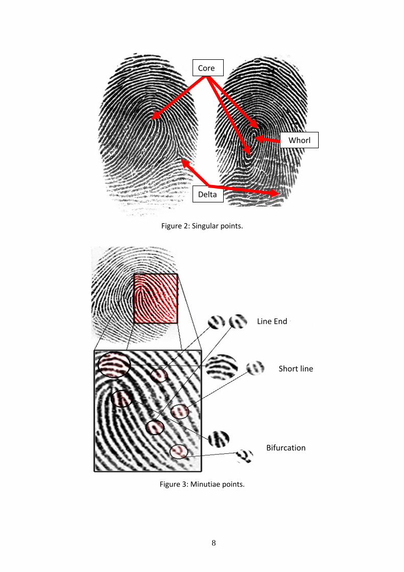
direction. Such areas of discontinuity are called singular points (Figure 2).

There are three types of singular points [20]: core (ridge lines make a 180

degree turnaround core point), delta (ridges from three directions and

connect in one point called delta) and whorl (ridge lines make a 360 degree

turn around whorl point).

8

Figure 2: Singular points.

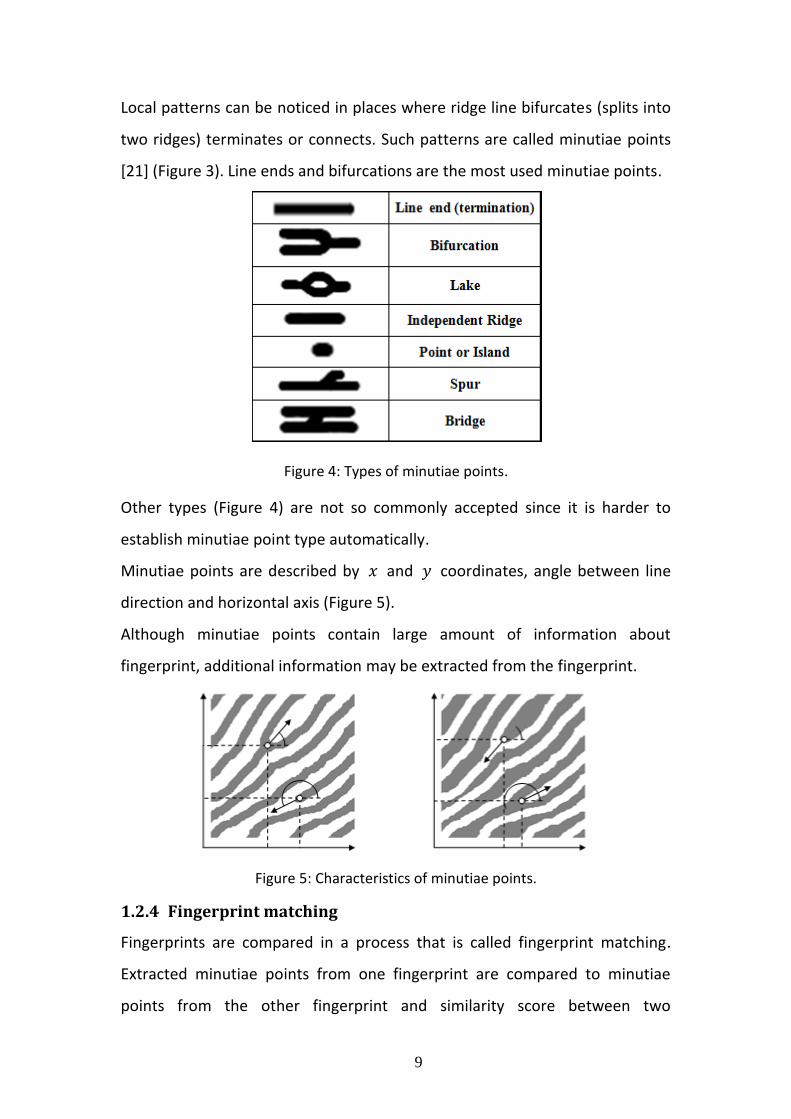
Figure 3: Minutiae points.

Delta

Whorl

Core

Line End

Bifurcation

Short line

9

Local patterns can be noticed in places where ridge line bifurcates (splits into

two ridges) terminates or connects. Such patterns are called minutiae points

[21] (Figure 3). Line ends and bifurcations are the most used minutiae points.

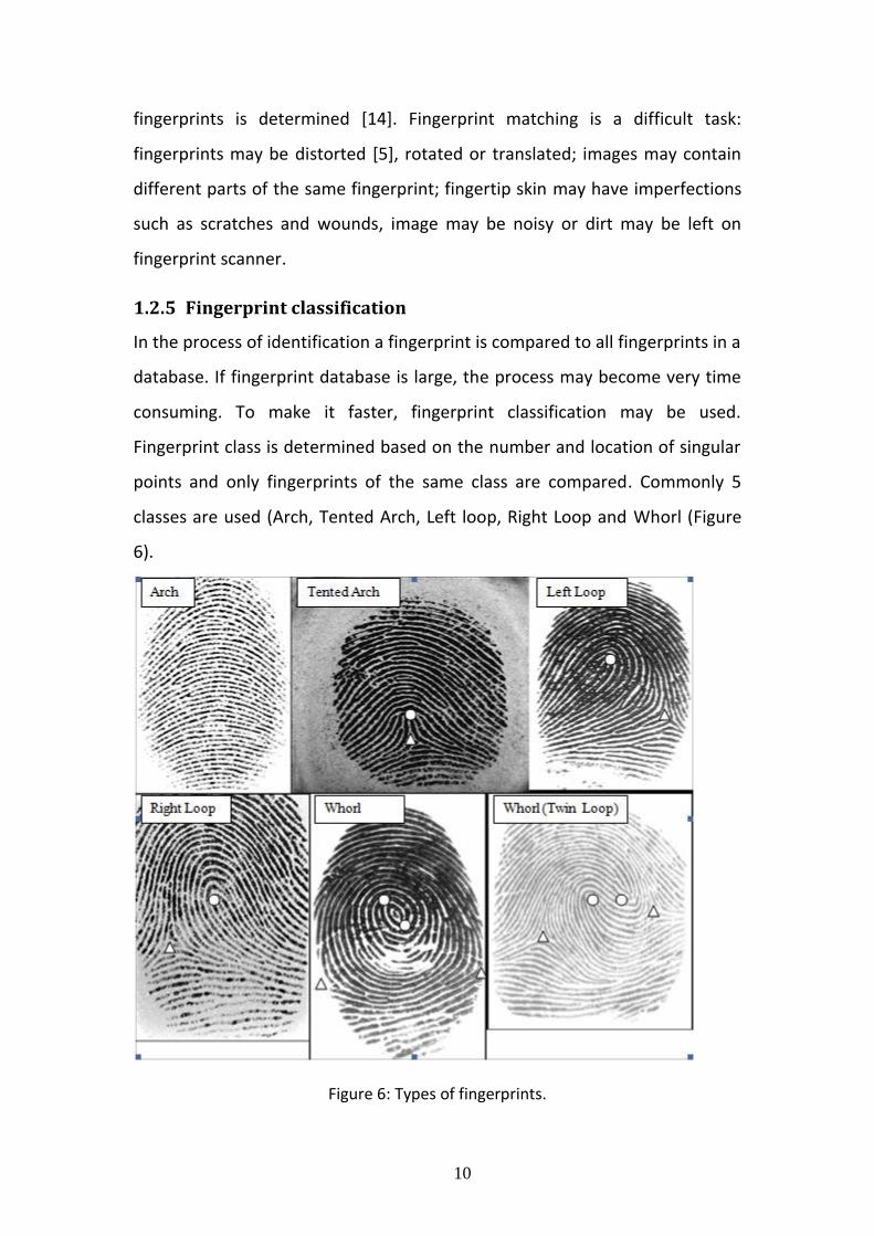
Figure 4: Types of minutiae points.

Other types (Figure 4) are not so commonly accepted since it is harder to

establish minutiae point type automatically.

Minutiae points are described by and coordinates, angle between line

direction and horizontal axis (Figure 5).

Although minutiae points contain large amount of information about

fingerprint, additional information may be extracted from the fingerprint.

Figure 5: Characteristics of minutiae points.

1.2.4 Fingerprint matching

Fingerprints are compared in a process that is called fingerprint matching.

Extracted minutiae points from one fingerprint are compared to minutiae

points from the other fingerprint and similarity score between two

10

fingerprints is determined [14]. Fingerprint matching is a difficult task:

fingerprints may be distorted [5], rotated or translated; images may contain

different parts of the same fingerprint; fingertip skin may have imperfections

such as scratches and wounds, image may be noisy or dirt may be left on

fingerprint scanner.

1.2.5 Fingerprint classification

In the process of identification a fingerprint is compared to all fingerprints in a

database. If fingerprint database is large, the process may become very time

consuming. To make it faster, fingerprint classification may be used.

Fingerprint class is determined based on the number and location of singular

points and only fingerprints of the same class are compared. Commonly 5

classes are used (Arch, Tented Arch, Left loop, Right Loop and Whorl (Figure

6).

Figure 6: Types of fingerprints.

11

Arch type fingerprints do not have any singular points. Tented arch type

fingerprints have two singular points: core and delta (delta is below core).

Loop type fingerprints also have two singular points: core and delta. Delta

point is located to the right (in case of left loop) or to the left (in case of right

loop) relative to core point. Whorl type fingerprints have two core and two

delta singular points. Ridge frequency and orientation maps (Figure 7) are

commonly used to evaluate fingerprint type automatically. Ridge frequency

map displays local ridge frequency and can also be used to separate

foreground from background.

Figure 7: Frequency map (left) Orients map (right).

1.2.6 Extraction of fingerprint features

Fingerprint features are extracted in feature extraction process. Typical

extraction algorithms use following image processing routines to extract

fingerprint features: segmentation (to remove background), normalization (to

stretch contrast), binarization (to distinguish ridges and valleys),

skeletonization (to make ridges thinner), and detection of minutiae points.

12

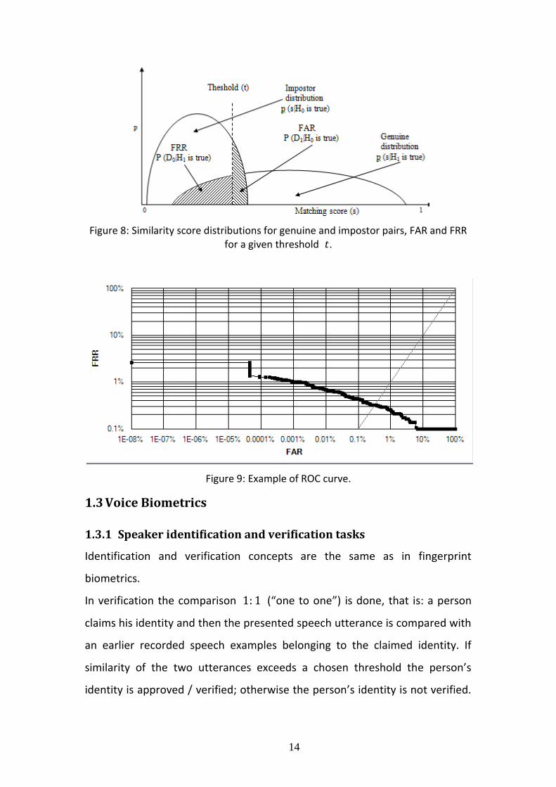
1.2.7 Fingerprint recognition performance evaluation

Biometric systems store biometric information (features) in the form of

template that characterizes a person. In case of fingerprints a template is a

file that keeps record of singular and minutiae points that were extracted

from a fingerprint image. The templates are stored in a database. During

verification input template from a person is compared to a stored template

and similarity is computed. Similarity score shows the

probability that templates and come from the same person. Null and

alternate hypotheses are:

, input template does not come from the same person as in stored

template T;

, templates and are from the same person.

The associated decisions are:

: person is not who he claims to be;

: person is who he claims to be. To make a decision, similarity score is

compared to a threshold . If similarity score is larger than threshold , the

decision is made that templates I and T come from the same person ( ). Two

types of error may occur:

Type I: false acceptance ( is decided when is true);

Type II: false rejection ( is decided when is true).

False Acceptance Rate (FAR) is the probability of type I error, False Rejection

Rate (FRR) is the probability of type II error:

To evaluate the performance of a biometric system on a specific database,

similarity score distribution must be collected on templates

from the same person (genuine similarity distribution), and distribution

on templates that come from different persons (impostor

similarity distribution). Figure 8 demonstrates FAR and FRR for a given

13

threshold . It is evident, that FAR is a percentage of impostor pairs whose

matching score is greater than or equal than threshold and FRR is a

percentage of genuine pairs whose similarity is less than threshold . Actually

FAR and FRR a functions depending on . Threshold is a tradeoff between

FAR and FRR. If threshold is increased, FAR decreases (system becomes more

secure), but at the same time FRR increases making it harder for a person to

be successfully identified. Additionally to FAR and FRR functions more simple

performance indicators are used:

Equal error rate (EER) is an error at such threshold t that FAR and FRR for that

threshold are equal.

Zero FRR is the lowest FAR at which no false rejections are made.

Zero FAR is the lowest FRR at which no false acceptances are made.

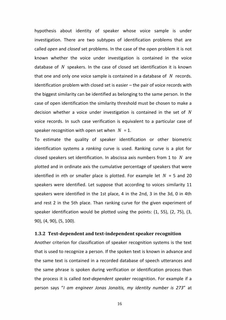
To compare different biometric systems FAR and FRR are computed for all

thresholds from 0 to maximum and a point (FAR(t), FRR(t)) is plotted on a

graphical plot for each threshold . The obtained curve demonstrates how

FAR depends on FRR for all possible thresholds is called receiver operating

characteristic (ROC) curve (Figure 9). ROC curve can be used to analyze such

biometric system parameters as FRR at given FAR (For example FRR@FAR =

0%, FRR@FAR = 0.1%, FRR@FAR = 0.01% or FRR at any other FAR). The lower

the ROC curve is, the better is the recognition performance. Although ROC

curve does not provide information about confidence intervals, this problem

is not significant since the number of impostor and genuine pairs is very high

even for small databases since each template in a database is verified against

all other templates. If a database consists of 1500 records (15 persons each

having 10 fingers scanned 10 times), the number of pairs is 1500*(1500-1) / 2

= 1124250.

14

Figure 8: Similarity score distributions for genuine and impostor pairs, FAR and FRR for a given threshold .

Figure 9: Example of ROC curve.

1.3 Voice Biometrics

1.3.1 Speaker identification and verification tasks

Identification and verification concepts are the same as in fingerprint

biometrics.

In verification the comparison (“one to one”) is done, that is: a person

claims his identity and then the presented speech utterance is compared with

an earlier recorded speech examples belonging to the claimed identity. If

similarity of the two utterances exceeds a chosen threshold the person’s

identity is approved / verified; otherwise the person’s identity is not verified.

15

Verification problem naturally arises in access control systems as in border or

immigration control services.

Any verification algorithm can make two types of errors: some percent of

genuine utterances may be rejected (not verified) and some percent of

speech utterances belonging to different persons may be claimed as being

genuine (belonging to the same person). The first type of error is called False

Rejection Rate (FRR) and the second is called False Acceptance Rate (FAR).

These two errors depend on chosen similarity threshold – higher thresholds

produce larger FRR and smaller FAR, and inversely the lower thresholds

produce smaller FRR but larger FAR. Graph of the parametric curve

, , where parameter t is the similarity

threshold, is called Detection Error Tradeoff (DET) curve. DET curve provides

visual representation of speaker verification algorithm performance. The

lower is the DET curve, the better is the quality of speaker verification

algorithm. DET curve is similar to a ROC curve that is commonly used in

fingerprint biometrics. The difference in the name appeared when fingerprint

biometrics and voice biometrics communities started using different names

for the same concept.

In identification comparison (“one to many” or “one to ”) is

performed, that is: a person does not claim his identity and the problem is to

find the most similar speaker among database of speakers or more

generally sort speakers in order of similarities to the speech utterance

under investigation. Person identification by voice has applications in

criminology or in security services (when for example, a mobile phone is

recorded and individuals that take part in conversations should be identified).

If there is no some additional information, the voices are arranged

according similarities of pairs of speech utterances where a pair consists

of voice sample under investigation and one of voice samples that are

recorded in a voice database. The pair with the largest similarity gives

16

hypothesis about identity of speaker whose voice sample is under

investigation. There are two subtypes of identification problems that are

called open and closed set problems. In the case of the open problem it is not

known whether the voice under investigation is contained in the voice

database of speakers. In the case of closed set identification it is known

that one and only one voice sample is contained in a database of records.

Identification problem with closed set is easier – the pair of voice records with

the biggest similarity can be identified as belonging to the same person. In the

case of open identification the similarity threshold must be chosen to make a

decision whether a voice under investigation is contained in the set of

voice records. In such case verification is equivalent to a particular case of

speaker recognition with open set when = 1.

To estimate the quality of speaker identification or other biometric

identification systems a ranking curve is used. Ranking curve is a plot for

closed speakers set identification. In abscissa axis numbers from 1 to are

plotted and in ordinate axis the cumulative percentage of speakers that were

identified in nth or smaller place is plotted. For example let = 5 and 20

speakers were identified. Let suppose that according to voices similarity 11

speakers were identified in the 1st place, 4 in the 2nd, 3 in the 3d, 0 in 4th

and rest 2 in the 5th place. Than ranking curve for the given experiment of

speaker identification would be plotted using the points: (1, 55), (2, 75), (3,

90), (4, 90), (5, 100).

1.3.2 Text-dependent and text-independent speaker recognition

Another criterion for classification of speaker recognition systems is the text

that is used to recognize a person. If the spoken text is known in advance and

the same text is contained in a recorded database of speech utterances and

the same phrase is spoken during verification or identification process than

the process it is called text-dependent speaker recognition. For example if a

person says “I am engineer Jonas Jonaitis, my identity number is 273” at

17

entrance and the same text is saved in utterances data base, speaker

recognition problem is text-dependent. Such recognition systems are used

more frequently in verification and require much shorter speech utterances

for speaker recognition. However text-dependent and even text-prompted

access control systems can be broken down by recorded examples of a person

speech utterance. A variation of text-dependent recognition may be used

when several different phrases of the same speaker are recorded in

utterances database and voice recognition system randomly asks to

pronounce a particular phrase during verification. Such systems belong to the

so called text-prompted systems and give additional flexibility to the speaker

verification process [60]. In the more general case a text-prompted system

can ask to pronounce any unknown in advance text.

In text-independent speaker recognition spoken and stored phrases have

different text content. Text-independent speaker recognition problem

naturally arises when we have a database of speech utterances of suspected

persons and a particular phrase or phrases recorded during phone call or by a

hidden microphone. One can remember recent examples of questionable Bin

Laden records where decision about speaker identity was done under text-

independent conditions. It is clear that speech utterances saved in speech

database should be sufficiently rich to cover possible phonetic range. If in

text-dependent speaker recognition requirement to a phrase duration is

about 10 sec., text-independent recognition requires speech examples 3-5

min. long.

Techniques that estimate text-dependent and text-independent speech

utterances use different approaches. In text-dependent speech recognition

systems Dynamic Time Warping (DTW) technique [61], [62] dominates. DTW

technique gives an elegant solution for compensation of variations in speed

with which the same phrase is pronounced. In speaker recognition using text-

independent speech examples Gaussian Mixture Model (GMM) [63], Vector

18

Quantization (VQ) [64], Arithmetic Harmonic Sphericity measure (AHS) [65],

and different variations of Hidden Markov Model (HMM) [66] dominate. Text-

independent recognition systems have an additional source of information

that is used in speaker recognition. This source is statistics of phonemes of

diphones used in free speech examples. The phonemes statistic can be

accumulated manually or using speech to text engines.

1.3.3 Speaker modeling techniques

A general structure of speaker recognition algorithms is presented in the

following scheme. For more detailed description of each step of the scheme

an overview on modern techniques that are used for speaker recognition was

used [67].

A typical scheme of speaker recognition system.

1.3.3.1 Speech signal processing, features

Any speech signal is first pre-emphasized. Pre-emphasizing filter enhances

high frequencies of the speech signal spectrum. The pre-emphasizing filter is

defined by the following formula:

The value of a parameter is taken from the interval and

depends on sampling rate of the speech signal. Some authors use signal

Target model Background model

Score normalization

Decision

Matching of models

Signal processing, feature extraction

19

adaptive values that depend on the contents of a frame. If features are

extracted using filter-banks or all-pass filters that have increasing resolution

with increase of frequency, application of pre-emphasizing filter is not

necessary. In general simple experiments with different values give

empirical answer to optimal a value. If pre-emphasizing gives only a small

increase in speaker recognition it is recommended not to apply this filter for

the speech signal. The initial speech signal is divided in frames and analysis is

done locally by applying a window to overcome boundary problem. A

windowed local speech signal is called a speech frame or just frame. Duration

of a frame is 20-30 milliseconds. The frames can have overlap and two

neighboring frames can be shifted in time 10 milliseconds back or forward.

These values are found empirically and are justified by an average physical

duration of time interval when the speech signal is approximately stationary.

In theory the shorter the frame the more stationary it is, however it would be

difficult to estimate the spectral content of a very short speech frame. 20

milliseconds duration allows estimating spectrum up to 100 hertz that is

sufficient for speaker recognition.

The Hamming and the Hanning windows are the most frequently used for

frame windowing. Both windows suppress boundary values that increases

signal-to-noise ratio in spectrum domain. The fast Fourier transform (FFT)

[68], [69] of the windowed signal represents the spectral content of the

frame. To apply FFT the samples of a frame should be padded by zeros to

have total number of samples that is a power of 2 (for example 256 or 512).

1.3.3.2 Mel Cepstrum

The modulus of the FFT represents power spectrum of the frame. The FFT

spectrum has a lot of fluctuations that can be reduced by application of a

filter-bank series. A fixed representative of the filter-bank averages FFT power

spectrum around central frequency. Standard deviation of the smoothing

filter increases with rise of central frequency that fits physiological property of

20

our hearing system. The parameters of the spectrum smoothing filter are

defined by their left, central, and right frequency. Filter can by triangular or

exponential type. In effort to copy the properties of our hearing system many

authors use the Bark/Mel scale for the central frequencies of the smoothing

filters. The central locations of the Mel scale are defined by the following

formula:

(

)

The presented formula is taken from [70]. More complicated versions of the

Mel scale exist but all formulas have a following property: for low frequencies

f (up to 1000) Mel scale converts frequency almost linearly and for high

frequencies the conversion becomes logarithmic.

Finally, the decimal logarithm is taken of this spectral envelope and is

multiplied by 20 in order to obtain the spectral envelope in decibels (dB). This

tradition comes from electronic engineers who use dB as a standard measure

unit. After this stage of the processing, a vector of features that encodes

spectral content of the frame is obtained. However such features have

redundant information and an additional transformation is performed to

reduce feature dimensionality. The cosine discrete transform is usually

applied here to produce cepstral coefficients [71], [72]:

∑ (

)

Here K is the number of power spectrum values smoothed on Mel scale

central frequencies and is the number of cepstral coefficients.

1.3.3.3 Linear prediction

In all-pole Linear Prediction (LP) model value of a signal is predicted by a

linear combination of its previous values [73]:

∑

21

where is the order of LP model; are linear prediction coefficients (LPC)

of the model; is a gain scaling factor and is the source for the present

input. The LPC parameters of LP approximation ∑ are

found by minimization of a sum of the squared approximation errors.

Traditionally the LP source is not modeled in speaker recognition that limits

the use of fundamental frequency to recognize speaker. This limitation can be

overcome by modeling of the source or by direct estimation of the

fundamental frequency and their statistics.

The LP model leads to the transfer function

( ∑

) ⁄⁄

where of the p-th order of all pole LP model. Mean

square error of the residuals is typically minimized because this

leads to more simple linear equations for the prediction of the coefficients

that are easily solved by computers.

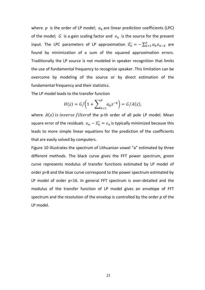
Figure 10 illustrates the spectrum of Lithuanian vowel “a” estimated by three

different methods. The black curve gives the FFT power spectrum, green

curve represents modulus of transfer functions estimated by LP model of

order p=8 and the blue curve correspond to the power spectrum estimated by

LP model of order p=16. In general FFT spectrum is over-detailed and the

modulus of the transfer function of LP model gives an envelope of FFT

spectrum and the resolution of the envelop is controlled by the order p of the

LP model.

22

Figure 10: Wave function of the Lithuanian vowel "a" (above) and its spectrum estimated by different methods (below).

1.3.3.4 LPC-based cepstral parameters

Coefficients of fixed order LP model are estimated for any speech frame. LPC

parameters are rarely used directly for speaker recognition. The prediction

coefficients are unstable in case of small perturbations of speech signal and

do not have a simple interpretation. It was discovered that some linear

combinations of the LP coefficients can give approximations of the cepstral

coefficients. If the order p of the LP model tends to infinity the

approximations tends to equalities [74].

Sou

nd

pre

ssu

re le

vel (

dB

/Hz)

Frequency (Hz)

23

The linear expressions that convert LPC to LP Cepstral Coefficients (LPC to

LPCC) are the following:

∑

∑

1.3.3.5 Additional transformations

Mel or LP Cepstral Coefficients allow a simple procedure for channel

compensation. Channel distortions can be modeled as additional filter that is

applied to the signal. Since the channel filter is approximately constant in time

and the cepstral coefficients correspond to the Fourier coefficients of the

logarithm of the power spectrum, the channel transfer function transforms

into an additional term which may be removed by subtracting mean values of

the cepstral coefficients. This operation is named cepstral mean subtraction

(CMS) and is often used to increase the tolerance of speaker recognition to

channel differences, differences in recording conditions, background noise,

etc. However CMS do note solves such problem as additional noise which has

no convolutive property. A partial solution for reduction of additive noise

problem can be equalization of variance of each cepstral component.

Cepstral coefficients do not contain information about dynamics of the

speech. For that purposes the so called delta (Δ) and delta-delta (ΔΔ)

parameters are added to cepstral coefficients. The delta and delta-delta

parameters are an approximation of first and second derivatives of the

cepstral coefficients as functions in time [75]. The derivatives can be

estimated by the following formulas:

∑

∑

,

∑

∑

,

24

where with upper index represents vector of cepstral coefficients of

the m-th frame and parameter = 1, 2 or 3. The first component of vector of

cepstral coefficients is not invariant to recording conditions and is

not included into features set; however the first component of

vectors becomes invariant to the level of loudness of recording

device and can be included into final features vector.

1.3.4 Models of Speakers and their matching

When speech utterance is represented as a sequence of feature vectors it is

called that features of the signal are extracted. To have possibility to compare

extracted features the same type of features are selected for target

(database) and for investigative (input) speech examples. However different

utterances may have different textual content, different duration and

therefore cannot be compared directly frame-by-frame. In this section a short

introduction to feature matching techniques is provided. Two groups of

measures that are used for estimation of speech utterances are known. The

first group constructs a statistical model for measured features vectors. If

features are dimensional vectors a density function that

maximizes likelihood of observed features of the frames is constructed. If at

authorization process a speech frame with features vector f is observed,

direct substitution of to gives likelihood of that frame for the target

speaker with the density function Such substitutions should be

done for each frame and an average value represents similarity

measure of the two speakers models. Much faster comparison of the two

voice samples can be done by constructing a density function for investigative

(input) voice record also and estimating the probability that two densities

correspond to the random source of features vector f. Another type of

measures directly compares pairs of features vectors that correspond to

different frames of the target (database) and investigative (input) voice and a

global measure of similarity is constructed from local comparisons of

25

similarity of pairs of frames. This technique is called template matching, it is

more intuitive, and in common, is more expensive. Both types of measures

have their merits and demerits, and therefore a combination of them is often

used.

1.3.4.1 Template Models

In the most simple template model only a single template , which is the

model target (database) speech record, is used. Template belongs to the

linear space of all possible feature vectors and can be defined as mean vector

of feature vectors of speech frames. Such approach minimizes mean square

Euclidean distance error between a fixed template and all frame feature

vectors. If we have feature vectors of M frames of a

target voice record, then target speaker template would be

∑

Distance between feature vector of an investigative (input) m-th frame

and target model is expressed by:

( ) √( )

Here is a feature components weighting matrix. Euclidean distance is

defined by identity matrix, covariance matrix of frame feature vectors define

Mahalanobis distance. If initial feature vectors are transformed to the space

which basis consists of orthogonal eigenvectors of the covariance matrix, the

Mahalanobis distance is equal to Euclidean distance and computational cost

of the latter is much smaller (proportional to the dimensionality of feature

vector) [76].

1.3.4.2 Dynamic Time Warping

If speaker recognition is text-dependent or text-prompted with vocabulary

covered in saved speech records database, template matching is an intuitive

approach and often used in speaker recognition. The idea is that even the

26

same phrases are pronounced by the same person, they sound more similar

than phrases pronounced by different speakers. Voice recognition is easier if

speakers cooperate with authorization system and pronounce personalized

utterances such as “I am Jonas Jonaitis, engineer, my personal number 375”

and “I am Petras Petraitis, my job position is in support division, personal

number 781”. It is natural to expect that average value of frame-to-frame

distance of both records of the same has good discriminative characteristic

for recognition of the claimed speaker. However in text-dependent and text-

prompted case small variations in speed by which utterances are spoken

appear. Dynamic Time Warping (DTW) [62] gives an elegant solution which in

some sense optimally arranges the frames that should by paired to compare

two utterances. The cost of DTW algorithm is moderate since distances

between all frames of two utterances should be estimated that makes

complexity quadratic. Suppose we have input voice features

vectors and target voice features vectors. Than DTW

algorithm gives non-decreasing set of indices

that minimizes with some additional

conditions the average distance ( ) ∑ ( )

Figure 11: Frame correspondences without alignment (left) and with DTW alignment (right).

Figure 11 illustrates identical alignment of frames of two curves

that have the same number of points (left part) and the one which minimizes

27

average distance between two curves (right part). Some attempts to explore

DTW method for text-independent speaker recognition are known, but since

DTW algorithm has quadratic complexity and text-independent speech

records are much longer than text dependent records, application of DTW

technique in such cases is limited.

1.3.4.3 Vector Quantization approach

The main drawback of DTW template matching approach is that this

technique does not work for text-independent speaker recognition. A direct

on templates matching of two speech samples would be estimation of

distances or similarities between all possible pairs of features vectors that

correspond to two speech utterances and minimization of the obtained

distances matrix by columns and rows and calculation of average minimal

distances. However such direct approach leads to big computational cost. For

example if we have two utterances 3, 5 minutes long with length and distance

between neighboring frames of 10 milliseconds, the total number frame pairs

similarity of which should be estimated will be 3x60x10 x 5x60x10 = 54 e 6

that is sufficiently big number even for modern computers. Vector

Quantization is an old well known technique which allows reducing initial

number of vectors by rounding them to centroids that contain the so called

codebook [98]. Vectors of codebook are usually formed by some clustering

procedure. The size of the codebook ranges in speaker recognition from 32 to

2048 and has tendency to grow recently. Let denote the codebook

constructed for target speaker vectors. Then the average quantization

distance of investigated voice feature vectors defines distance between the

two speakers. Formally for the distance such expression is used:

∑ ( )

28

The vector quantization technique reduces computational costs and is often

used as one of similarity/distance measure for voice comparison. To further

increase the speed of comparison of two voice records, the features vectors

of both vectors can be quantized and distances or similarities between code

words of the two vector codebooks can be used. However such approach

decreases the quality of speaker recognition. Sometimes such double

quantization approach is used for initial selection of most similar pairs of

records that are further investigated by traditional Vector Quantization

modeling.

1.3.4.4 Nearest Neighbors method

Nearest neighbors (NN) method combines strength of DTW and VQ methods.

Unlike the VQ method, NN method keeps all features vectors of the target

data [98]. For each input frame the most similar enrolled target frame is

found and for each enrolled target frame the most similar input frame is

found and the two series of minimal distances are averaged. This method is

the most computationally complex but it gives the best results in of text-

independent speaker recognition when the recognition is done by template

matching methodology.

1.3.4.5 Stochastic models

Template methods work well for text-dependent speaker recognition

however they are computationally complex expensive and not state of the art

quality when text-independent recognition is needed. In stochastic approach

a density function that maximizes the likelihood to observe the same feature

vectors for input phrases that are observed for target speakers is constructed.

For each target speaker a separate density function is constructed. Then the

estimation of the likelihood to observe feature vectors of unknown speaker

for all target models gives the measure of probability that the unknown input

speaker has the same identity as a target speaker. So we have set of

29

conditional probability distribution functions with the number of conditions

equal to the number of target speakers. Conditional probability density

function (pdf) of a target speaker is estimated from the set of training

features vectors and can be parametric on non-parametric. In any case

(parametric or non-parametric pdf) probability that feature vectors of

unknown speaker are generated by the claimed target model can be

estimated. This probability gives not normalized matching scores. To build

parametric model, a specific form of pdf should be assumed and then free

parameters of the model are determined by maximization of likelihood of

observed training features vectors. One possible assumption can be made

that the pdf is the multivariate normal density function. Then free parameters

of the model would be mean vector and covariance matrix C of the

multivariate normal distribution. In this case value

√

.

Here K is dimension of frame features vector, is determinant of the

covariance matrix. Having features training vectors mean

vector and covariance matrix of target model can be estimated by the

following expressions:

∑

∑ ( )

Here “ ” denotes point-wise multiplication. However multivariate normal

distribution is a very simple approximation of real training vectors and

therefore Gaussian Mixture Model (GMM) in which density function is a

normalized sum of a few different multivariate normal distributions is used.

More detailed description of this model is given in next chapter. Although

strictly speaking speech frames do not provide independent feature vectors it

is assumed that they are independent. Such assumption allows estimating

30

conditional probability of unknown speaker simply by multiplying frames

probabilities.

Another very popular stochastic model is Hidden Markov Model (HMM) [97].

Hidden Markov Model is a double embedded stochastic process in the sense

that the stochastic process is not directly observable. The HMM is defined by:

1. Finite set of states

2. NxN matrix of transition probabilities , which means “transit

at next time moment to the state if we were at state at

current time”. It is assumed that transition probabilities do not

depend on time.

3. Finite set of observable symbols ,

4. matrix of probabilities which means “probability to

observe symbol at state ,

5. probabilities that define state probabilities at initial

moment.

Having observations set and HMM it is easy to calculate probability of such

observation. However in practice HMM should be constructed from

observations. For fixed parameter the rest of HMM parameters and

sequence of states are chosen by maximizing probability to have the

observations set under the model and the states sequence.

These two problems are solved using Baum-Welch and Viterbi algorithms 98.

1.3.4.6 Gaussian Mixture Model

The most popular stochastic model that is successfully applied for many years

in speaker recognition is Gaussian Mixture Model (GMM). The authors of this

method are Reynolds and Rose [80]. In this model, pdf function is modeled by

the expression:

∑ ,

where √

(

)

31

is shifted multivariate normal distribution and

∑

are weights of the shifted and scaled normal distributions. The complete

Gaussian mixture density has I mean K dimensional vectors, K x K covariance

matrices and positive weights. However, it is often assumed that covariance

matrices have simple structure, for example diagonal, that save memory

required for model and simplifies the estimation of the model. GMM model

has simple interpretation. Speech signals are composed by different

phonemes that can by clustered in feature space and each component of

GMM density can represent a particular phoneme and the weights of mixture

represents frequency/probability of occurrence of that phoneme. Mean

vectors define acoustic positions of the phonemes and covariance

matrices sharpness of localization of phonemes around their acoustic

centre. GMM has advantage over VQ approach since the latter can be

interpreted as an approximation of pdf by a discrete histogram with centers in

code words. On the other hand, code words of VQ can be used for initial

positions of mean vectors that are later tuned by an iteration process that

maximizes a posteriori probability to observe training features vectors.

Let represents parameters of the GMM. Than

having target training features vectors the GMM parameters

are found by maximizing the a posteriori probability

( ) ∏ ( )

The a posteriori probability highly non-linearly depends on the model

parameters that require applying some iterative process for maximization of

the probability. Having constructed GM target model the measure of

correspondence of unknown voice to the target voice is estimated by

( ) ∏ ,

where are feature vectors of unknown speaker voice utterance.

32

1.3.5 Speaker recognition by Lithuanian authors

The most contribution to speaker recognition is done by Antanas Leonas

Lipeika with co-authors. In his and J. Lipeikiene first paper [81] speaker

identification problem is considered. In [82] a modification of VQ method for

speaker identification is proposed. The main contribution was in modification

of quantization algorithm that allowed increasing codebook by one and tune

it for optimization of speaker identification quality. In [83] a notion of pseudo

stationary segments was proposed and applied for speaker recognition.

Pseudo stationary segments were found by joining adjacent frames that have

similar spectral content. Similarities of spectral contents were estimated by

likelihood ratio distance [84]. When pseudo stationary segments are found, a

direct minimization of a likelihood distance is done for fixed segments of

investigative (input) voice versus all possible target (database) segments and,

vice versa, pseudo stationary segment of target voice is fixed and the most

similar to that segment investigative segment is found. Average values of

likelihoods of the pseudo stationary signals are used as final similarity

measure. In [85] an idea of application of LPC residual signal to increase the

quality of speaker recognition was proposed. It was shown that fusion of

ordinary speaker similarity measures with the ones estimated for LPC residual

signal can increase speaker recognition quality. In this paper usual Euclidean

metrics calculated on LPC derived cepstral coefficients were investigated and

likelihood ratio distance was mentioned. It was shown that for both metrics

an increase in speaker recognition quality after fusion of the two types of

feature metrics is observed. In [86] the possibilities of DTW based techniques

for speaker recognition were investigated. In [87] the details of GMM were

analyzed and a compact set of features that are estimated on the base of Line

Spectral Pairs (LSP) that are derived from marginal LPC variations was

proposed. It was shown that dimensionality of features can be reduced two or

more times compared to a conventional cepstral features without significant

33

loss in speaker recognition quality. Another work worth mentioning is [88],

where the usage of consonant-vowel diphones for speaker discrimination was

proposed.

1.4 Problem Relevance

It is easy to notice that biometric technologies are spreading across the world.

Even low cost notebooks and mobile phones have integrated fingerprint

scanners and users can log on with fingerprint instead of password.

Integrated webcams are used to identify a person by face, and microphones

are used to provide access to the system by the voice. All these technologies

provide faster and reliable access to data, bank account or computer than

password, because passwords can be stolen, forgotten, lost or unlocked by

specific software. These are the reasons why many universities, companies

and institutions invest time and money in research and development of

biometric algorithms.

Several international competitions were arranged to compare different

biometric algorithms and track progress in biometric research: FVC (FVC 2000,

FVC 2002, FVC 2004, FVC 2006 and FVC ongoing), NIST (National Institute of

Standards and Technology) MINEX (MINEX, MINEX II and Ongoing MINEX) and

PIV for fingerprints; NIST Face Recognition Vendor Tests (FRVT) for faces; NIST

Speaker Recognition Evaluation (SRE) for voice biometrics; NIST Iris Challenge

Evaluation (ICE), Independent Testing of Iris Recognition Technology (ITIRT)

for irises are the largest and most known biometric competitions. These

competitions show that in spite the progress in such aspects as reliability,

speed and interoperability is impressive, there are many difficult problems

left to overcome.

All biometric technologies are dependent on input quality: If obtained

fingerprint image is noisy, low contrast or deformed; recorded voice phrase is

of low volume or very short, iris image is obstructed by eyelids, reflections or

glasses, face image is acquired in poor lightning conditions or using low

34

quality camera, the task of verification becomes more difficult. The main

challenge of modern biometric algorithms is to overcome these difficult

conditions and extract as much data as possible. Innovative methods help

algorithm developers better understand the weaknesses of their algorithms

and address them. Algorithm developers have to take into consideration that

when the popularity of biometric technology increase, requirements to

algorithm accuracy also increase. Error rate of one percent may be suitable

for a small company using time attendance system based on biometrics, but

will make a lot of problems to a bank with millions of customers or during

elections to prevent multiple voting.

This work is about fingerprint and voice biometrics. Fingerprint biometrics is

the most popular biometrics: fingerprint scanners are cheap, easy to use and

the process of verification is fast.

Voice biometrics is the most available biometrics, because no additional

hardware is needed. Most computers have audio interface with possibility to

plug microphone, microphones are integrated into webcams, headphones

and mobile phones.

1.5 Research Objects

The thesis research objects are: performance evaluation of fingerprint

extraction algorithm using fingerprint synthesis, fingerprint matching method

that is able to match deformed fingerprints, person identification using voice

and fusion of both biometrics.

1.6 The Objectives and Tasks of the Research

The aim of the research was to complexly analyze research area and address

difficult problems. In the first part of the work fingerprint extraction algorithm

development problems are analyzed and fingerprint image synthesis is

suggested to overcome that problems. In the second part of the work

fingerprint matching algorithm problems are analyzed and new matching

35

algorithm is proposed to deal with them. New person identification by voice

method is addressed in the third part of the work and multibiometrics using

fingerprints and voice is proposed to increase identification accuracy.

1.7 Scientific Novelty

The new method of fingerprint image synthesis is introduced in first chapter.

Differently from already existing synthesis methods it can generate fingerprint

images with predefined features. Such images with known characteristics

allow evaluating the performance of fingerprint extraction algorithm

independently from fingerprint matching algorithm. A new practical

application for synthetic fingerprints is suggested: they can be used to

estimate the quality of images in a given database or the quality of a

fingerprint scanner.

New fingerprint matching algorithm that is described in the second chapter

does not perform fingerprint registration (evaluation of rotation and

translation) and is capable to match fingerprints with elastic deformations.

Multibiometrics using new person identification by voice method and new

fingerprint matching method is described in next chapters. The performance

was analyzed using specially prepared multibiometric database.

This work is the first attempt to prove that there is no correlation observed

between similarities based on fingerprints and similarities based on voice.

Such independence of two biometrics means that they can be successfully

combined into multibiometrics.

1.8 Practical Importance of the Work

Methods described in this work can be used to solve many difficult tasks.

Fingerprint image synthesis (chapter 2) can be used to generate large

fingerprint databases, to evaluate the performance of fingerprint extraction

algorithm. Since it is possible to generate a fingerprint image with pre-defined

properties and features, it becomes easy to evaluate such properties of

36

fingerprint extraction algorithm as stability to noise and accuracy of extracted

features.

New fingerprint matching method (chapter 3) allows accurate matching of

plain and rolled fingerprints with elastic deformations that are common in

rolled fingerprints and sometimes occur in plain fingerprints.

Multibiometrics using fingerprints and voice (chapters 4 and5) can provide

more flexible and accurate way of person identification.

1.9 Approval of Research Results

Research results were published in valuable international journal Informatica.

The conference papers were presented and an oral presentation in

INFORMATION TECHNOLOGIES (IT2010) conference was done.

1.10 Defended propositions

1. New fingerprint image synthesis method can generate

fingerprints with predefined features. Such fingerprints can be

used to test and develop biometric systems.

2. Fingerprint image synthesis uses iterative convolution with large

kernel that is a very time consuming operation. An optimization

that speeds up synthesis process several times was presented.

3. A method to evaluate the performance of fingerprint extraction

algorithm using synthetic fingerprints can be used evaluate

extractor’s performance.

4. Fingerprint matching method that does not perform fingerprint

registration and is able to match deformed plain and rolled

fingerprints with better accuracy.

5. New speaker identification method outperforms traditional

speaker identification methods.

37

6. Since fingerprint and voice similarities do not correlate much,

multibiometric using both fingerprints and voice can further

increase identification accuracy.

1.11 Publications

International journals which are included into the International Master

Journal List (ISI):

1. Andrej Kisel, Alexej Kochetkov, Justas Kranauskas (2008).

Fingerprint Minutiae Matching without Global Alignment Using

Local Structures INFORMATICA, 2008, Vol. 19, No. 1, 31-44 ISSN

0868-4952.

2. Algirdas Bastys Andrej Kisel, Bernardas Salna (2010). The Use of

Group Delay Features of Linear Prediction Model for Speaker

Recognition INFORMATICA, 2010, Vol. 21, No. 1, 1-12 ISSN 0868-

4952.

International journals which are included in the Scientific Master Journal

Proceeding List (ISI):

1. Andrej Kisel (2010). Fast Fingerprint Image Synthesis.

Proceedings of 16th International Conference on Information

and Software Technologies. April 21st - 23rd 2010, Kaunas

University of Technology, Lithuania, ISSN 2029-0063 pp. 107-

115.

Journal submissions under review:

1. Andrej Kisel (2010). Multibiometrics using fingerprints and

voice. Information technology and control, Kaunas University of

Technology.

1.12 Outline of the Thesis

The thesis consists of 3 main parts: fingerprint biometrics (chapters 2 and 3),

voice biometrics (chapter4) and multibiometrics (chapter 5).

38

The 2nd chapter describes fast fingerprint image synthesis method that can

be used to create large fingerprint databases and to evaluate the

performance of fingerprint extraction methods.

The 3d chapter is devoted to a fingerprint matching method that is robust to

deformations and does not perform fingerprint alignment.

The 4th chapter introduces the use of group delay features of linear

prediction model for speaker recognition.

The 5th chapter presents multibiometrics using fingerprints and voice.

The 6th chapter completes thesis with brief summary and conclusions. At the

end of the work a bibliography list is presented.

2 Fingerprint image synthesis

This chapter presents a fingerprint synthesis method that can generate a

fingerprint with predefined minutiae points. Fingerprint type is chosen

randomly and singular points positions and quantities are chosen randomly

according to the fingerprint type. Orientation map is generated using

fingerprint orientation model. Ridge frequency map is generated. Initial image

with drawn minutiae points that are oriented by orientation map is

constructed. Iterative filtering of the initial image with Gabor filters that are

oriented using orientation map and constructed using frequency map

produces fingerprint image with minutiae points located at the predefined

positions. An optimization of the iterative filtering is described. Synthetic

fingerprint images are used to evaluate extraction algorithm's stability to

noise. A measure of extraction algorithm’s robustness to noised fingerprint

images is proposed.

2.1 Introduction

Much attention is being paid to different biometric algorithms such as person

identification by unique features. Fingerprint identification is one of the most

39

popular ways to identify a person and much research is done in this area of

biometrics. Identification process consists of fingerprint image acquisition,

feature extraction and feature matching.

Different methods to evaluate algorithm performance are proposed [38], [39],

[40], [41] and most of them use fingerprint databases such as NIST SD4 [42]or

NIST SD14[43] to calculate accuracy. Features are extracted in enrollment

phase [44], [45] and then extracted features are matched against each other

in matching phase [13] [18] [46] to calculate Receiver Operating Characteristic

(ROC), Detection Error Trade-off (DET) or other statistics [47]. Many

competitions [18], [48] have been arranged to analyze and benchmark

different commercial and academic algorithms. The biggest and most

thorough of them was NIST arranged competition MINEX [49]: Vendors could

send their extraction or matching algorithms and best extractors and

matchers were selected. Majority of vendors send both algorithms and it is

interesting, that in many cases matching algorithms performed better with

extractors from the same vendors (it can be seen from scenario 1 in MINEX

report [49]). It can be easily explained, since many vendors develop both

matcher and extractor and they know about typical problems of their

extractors and can compensate for them in matching phase. It is hard to

develop an accurate extraction algorithm because it is hard to evaluate it

without a good matcher and since most vendors develop both algorithms,

they are not sure that even if performance of their matcher or extractor is

good enough, it will be good when used with other extractor (or matcher).

Estimation of biometric algorithms performance expressed in ROC or DET

curves depends on database of fingerprint images, quality of extraction and

quality of matching algorithm. To have the possibility to estimate extractor

and database quality separately from matching routine, we propose to utilize

synthesized fingerprints images. Synthesized images can serve as a reference

or as an ideal database that allows introducing some quantitative quality

40

measures for estimation of extractor’s performance for a particular database.

If one extractor is applied on several fingerprint image databases, the

database quality can be associated with the proposed quality measure. The

situation is similar to situation when the quality of several extraction

algorithms can be compared if same database for each extractor is used to

calculate statistics.

The ROC and DET characteristics of extracting algorithm can be replaced by a

quality measure that accounts information about exact positions, types and

orientations of minutiae. To have fingerprints images with predefined

minutiae points, we extend SFINGE fingerprint image synthesis method [50].

2.2 SFINGE

Different synthesis methods were analyzed [50], [51], [52] and SFINGE [50]

was chosen as a base method. It is well described and its ability to generate

finger-like images was tested in fingerprint verification competitions

(FVC2000 [38] FVC2002 [18] FVC2004 [48] and FVC2006), in which one of four

databases was generated synthetically. Generated fingerprints look like real

ones, and identification algorithms performance is similar to performance

obtained on real fingerprints.

SFINGE (Synthetic Fingerprint Generation) consists of several steps:

Fingerprint form generation, fingerprint type and orientation map generation,

density map generation, ridge generation.

2.2.1 Fingerprint form

Fingerprint generation is starting by fingerprint form determination.

Fingerprint form can be described by many different methods. For example, it

can be described by an ellipse, or by a square with rounded corners. SFINGE

method uses five coefficients, which can be generated randomly, or inserted

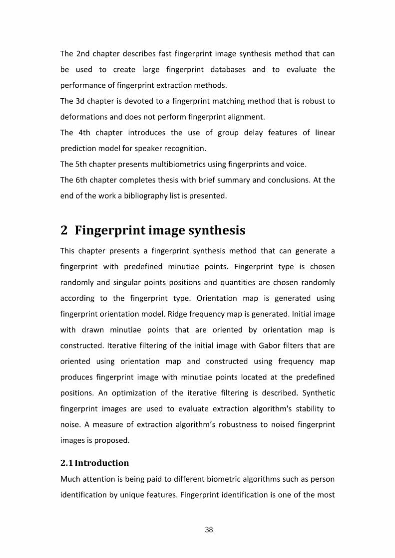
manually or derived from the real fingerprint (Figure 12).

41

Figure 12: Five coefficients that describe fingerprint form (left) and fingerprints of different form (right).

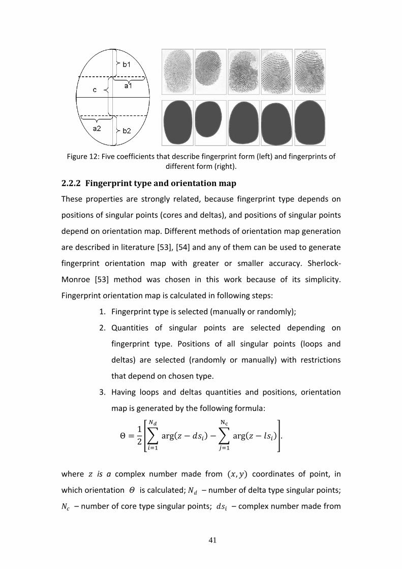
2.2.2 Fingerprint type and orientation map

These properties are strongly related, because fingerprint type depends on

positions of singular points (cores and deltas), and positions of singular points

depend on orientation map. Different methods of orientation map generation

are described in literature [53], [54] and any of them can be used to generate

fingerprint orientation map with greater or smaller accuracy. Sherlock-

Monroe [53] method was chosen in this work because of its simplicity.

Fingerprint orientation map is calculated in following steps:

1. Fingerprint type is selected (manually or randomly);

2. Quantities of singular points are selected depending on

fingerprint type. Positions of all singular points (loops and

deltas) are selected (randomly or manually) with restrictions

that depend on chosen type.

3. Having loops and deltas quantities and positions, orientation

map is generated by the following formula:

[∑

∑

]

where is a complex number made from coordinates of point, in

which orientation is calculated; – number of delta type singular points;

– number of core type singular points; – complex number made from

42

i-th delta coordinates; – complex number made from j-th loop

coordinates; – complex number argument;

Orientation is calculated in each pixel of fingerprint image (Figure 13).

Figure 13: Example of orientation maps for different type fingerprints.

2.2.3 Ridge density map generation

Ridge density map is generated using following information about fingerprint

characteristics: Default distance between ridges is 9 pixels (here and below

we assume that scanner’s resolution is 500 pixels-per-inch (DPI)), ridge

frequency is lower on the top of the image, and lower on the bottom [20].

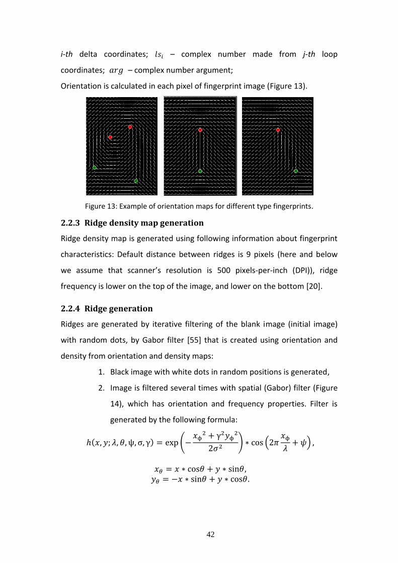
2.2.4 Ridge generation

Ridges are generated by iterative filtering of the blank image (initial image)

with random dots, by Gabor filter [55] that is created using orientation and

density from orientation and density maps:

1. Black image with white dots in random positions is generated,

2. Image is filtered several times with spatial (Gabor) filter (Figure

14), which has orientation and frequency properties. Filter is

generated by the following formula:

(

) (

)

43

In this equation, represents the wavelength of the cosine factor,

represents the orientation of the normal to the parallel stripes of a Gabor

function, is the phase offset, is the sigma of the Gaussian envelope and

is the spatial aspect ratio, and specifies the ellipticity of the support of the

Gabor function.

Figure 14: Gabor filter.

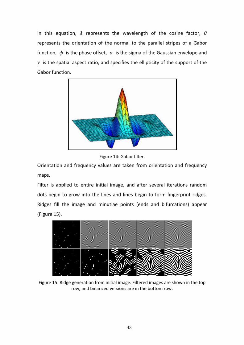
Orientation and frequency values are taken from orientation and frequency

maps.

Filter is applied to entire initial image, and after several iterations random

dots begin to grow into the lines and lines begin to form fingerprint ridges.

Ridges fill the image and minutiae points (ends and bifurcations) appear

(Figure 15).

Figure 15: Ridge generation from initial image. Filtered images are shown in the top row, and binarized versions are in the bottom row.

44

2.2.5 Analysis

An algorithm was implemented, and after experiments and research it was

modified to generate minutiae points not in random positions, but in

predefined ones. The following section describes a method that is fast and

can generate images with minutiae in given positions.

2.3 Modified SFINGE Method

Since method is based on SFINGE method, steps like orientations map

calculation and filtration are not described here once more. This section is

focused on the differences between original and modified method.

Main steps of fingerprint generation are:

1. fingerprint type is chosen (randomly or manually);

2. orientations (Figure 13) are generated;

3. Gabor filters of orientations that present in orientations image

are generated before filtering to speed up generation;

4. initial image is constructed;

5. initial image is filtered with Gabor filters that are oriented by

orientation image.

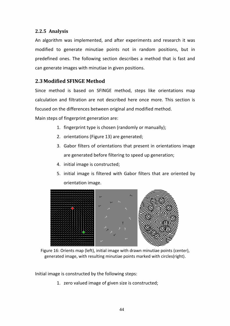
Figure 16: Orients map (left), initial image with drawn minutiae points (center),

generated image, with resulting minutiae points marked with circles(right).

Initial image is constructed by the following steps:

1. zero valued image of given size is constructed;

45

2. coordinates (positions) and types of minutiae points are

generated randomly or selected manually;

3. small images of minutiae are drawn on the initial image in the

selected positions so that minutiae orientations are aligned with

orientation map.

There are two types of minutiae points – line ends and bifurcations. Since

these types are invertible (line end is a bifurcation on the inverted image), a

bifurcation is drawn using positive (+1) value pixels, and line end is drawn

using negative (-1) value pixels (Figure 16 (center)).

The most straightforward way to generate a fingerprint is to filter the Initial

image with Gabor filters that are oriented by orientation image (Figure 13),

but since responses of Gabor filters are calculated in every pixel, it is a

computationally complex operation. An optimization was implemented to

perform iterative filtering only in those pixels that are required in current

iteration to generate a fingerprint. The main idea of the improvement is to

start filtering from positions of drawn minutiae and near it, and to extend

filtering area until entire image is generated. For example, if Gabor filter is 10

pixels wide, then in the first iteration pixels that are from 0 to 10 pixels away

from the drawn minutiae points are filtered, in the second iteration – pixels

that are from 1 to 11 pixels away from drawn minutiae points are filtered, in

third iteration – pixels that are from 2 to 12 pixels away from drawn minutiae

points are filtered, in fourth iteration – from 3 to 13 pixels away, and so on,

until the fingerprint is generated (no pixels are left to filter). To perform fast

calculation of distances to minutiae points, Euclidean Distance Map (EDM)

[56] is calculated from initial image. The EDM map is an image, and value of

each pixel indicates the distance to the nearest object (drawn minutiae point).

The order of filtering can be easily calculated from EDM. In the first filtering

iteration only pixels that have values from 0 to 10 in EDM are filtered, in

second filtering iteration only pixels with values from 1 to 11 in Euclidean

46

Distance Map are filtered in initial image, in third iteration only pixels with

values from 2 to 12 are filtered, in fourth iteration – from 3 to 13 and so on.

(Figure 17 shows an example)

Figure 17: Iterations of generation. An area that is white is filtered n each iteration.

Filtering is performed by applying Gabor filter (orientation is taken from

orientation map, frequency is taken from the frequency map) to each pixel

of the initial image in the order that is calculated from EDM.

Generated image can be noised or transformed after generation to provide it

more natural look.

The described optimization speeds up generation process more than 5 times

comparing to a straightforward version.

The resulting generation speed is more than 2 fingerprints per seconds on

Intel Core 2 Duo 6600 processor.

It can be noticed that though some additional minutiae points appear in result

image, all initial minutiae points are present and location, direction and type

of them are the same as in the initial image.

Similar synthesis approach was independently used in [57] with the aim to

investigate the possibility of fingerprint reconstruction from standard

template. The main differences in generation process are summarized in the

following table (Table 1):

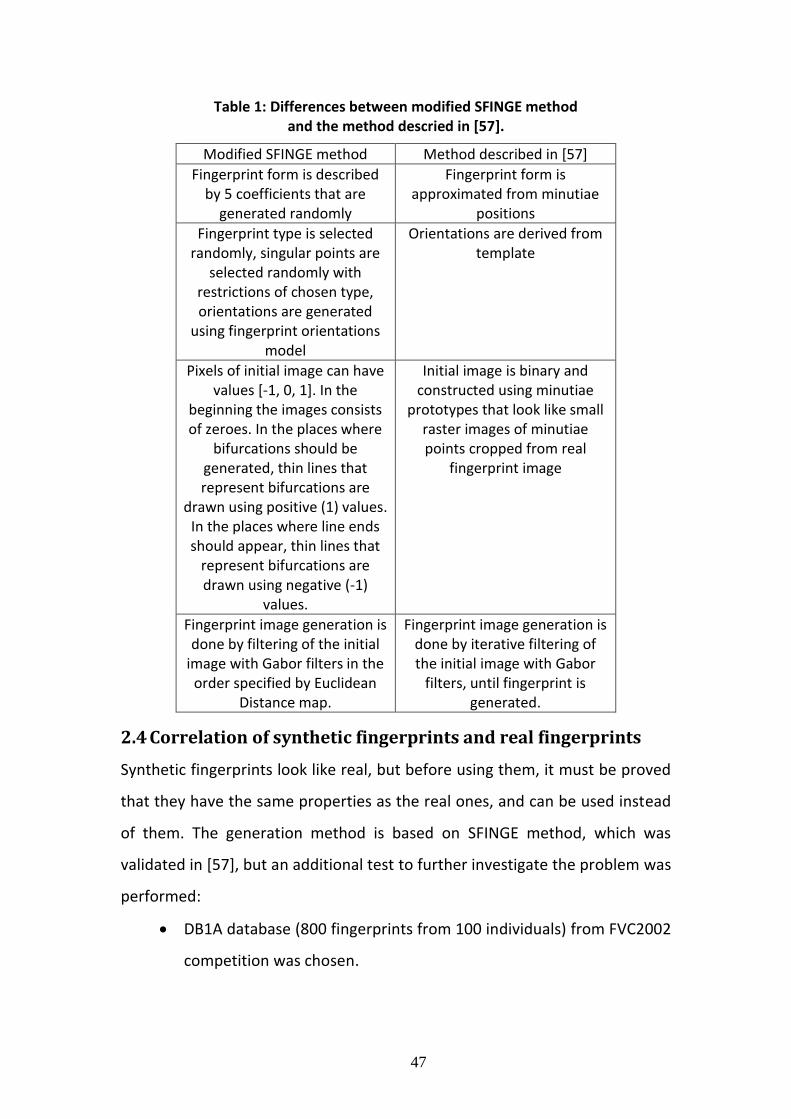
47

Table 1: Differences between modified SFINGE method and the method descried in [57].

Modified SFINGE method Method described in [57]

Fingerprint form is described by 5 coefficients that are

generated randomly

Fingerprint form is approximated from minutiae

positions

Fingerprint type is selected randomly, singular points are

selected randomly with restrictions of chosen type, orientations are generated

using fingerprint orientations model

Orientations are derived from template

Pixels of initial image can have values [-1, 0, 1]. In the

beginning the images consists of zeroes. In the places where

bifurcations should be generated, thin lines that represent bifurcations are

drawn using positive (1) values. In the places where line ends should appear, thin lines that

represent bifurcations are drawn using negative (-1)

values.

Initial image is binary and constructed using minutiae

prototypes that look like small raster images of minutiae points cropped from real

fingerprint image

Fingerprint image generation is done by filtering of the initial

image with Gabor filters in the order specified by Euclidean

Distance map.

Fingerprint image generation is done by iterative filtering of the initial image with Gabor

filters, until fingerprint is generated.

2.4 Correlation of synthetic fingerprints and real fingerprints

Synthetic fingerprints look like real, but before using them, it must be proved

that they have the same properties as the real ones, and can be used instead

of them. The generation method is based on SFINGE method, which was

validated in [57], but an additional test to further investigate the problem was

performed:

DB1A database (800 fingerprints from 100 individuals) from FVC2002

competition was chosen.

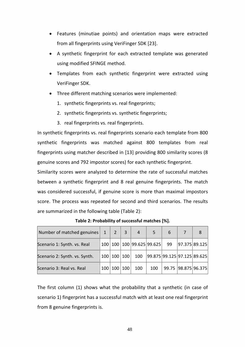
48

Features (minutiae points) and orientation maps were extracted

from all fingerprints using VeriFinger SDK [23].

A synthetic fingerprint for each extracted template was generated

using modified SFINGE method.

Templates from each synthetic fingerprint were extracted using

VeriFinger SDK.

Three different matching scenarios were implemented:

1. synthetic fingerprints vs. real fingerprints;

2. synthetic fingerprints vs. synthetic fingerprints;

3. real fingerprints vs. real fingerprints.

In synthetic fingerprints vs. real fingerprints scenario each template from 800

synthetic fingerprints was matched against 800 templates from real

fingerprints using matcher described in [13] providing 800 similarity scores (8

genuine scores and 792 impostor scores) for each synthetic fingerprint.

Similarity scores were analyzed to determine the rate of successful matches

between a synthetic fingerprint and 8 real genuine fingerprints. The match

was considered successful, if genuine score is more than maximal impostors

score. The process was repeated for second and third scenarios. The results

are summarized in the following table (Table 2):

Table 2: Probability of successful matches [%].

Number of matched genuines 1 2 3 4 5 6 7 8

Scenario 1: Synth. vs. Real 100 100 100 99.625 99.625 99 97.375 89.125

Scenario 2: Synth. vs. Synth. 100 100 100 100 99.875 99.125 97.125 89.625

Scenario 3: Real vs. Real 100 100 100 100 100 99.75 98.875 96.375

The first column (1) shows what the probability that a synthetic (in case of

scenario 1) fingerprint has a successful match with at least one real fingerprint

from 8 genuine fingerprints is.

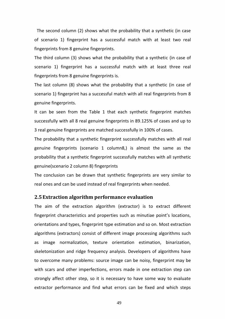
49

The second column (2) shows what the probability that a synthetic (in case

of scenario 1) fingerprint has a successful match with at least two real

fingerprints from 8 genuine fingerprints.

The third column (3) shows what the probability that a synthetic (in case of

scenario 1) fingerprint has a successful match with at least three real

fingerprints from 8 genuine fingerprints is.

The last column (8) shows what the probability that a synthetic (in case of

scenario 1) fingerprint has a successful match with all real fingerprints from 8

genuine fingerprints.

It can be seen from the Table 1 that each synthetic fingerprint matches

successfully with all 8 real genuine fingerprints in 89.125% of cases and up to

3 real genuine fingerprints are matched successfully in 100% of cases.

The probability that a synthetic fingerprint successfully matches with all real

genuine fingerprints (scenario 1 column8,) is almost the same as the

probability that a synthetic fingerprint successfully matches with all synthetic

genuine(scenario 2 column 8) fingerprints

The conclusion can be drawn that synthetic fingerprints are very similar to

real ones and can be used instead of real fingerprints when needed.

2.5 Extraction algorithm performance evaluation

The aim of the extraction algorithm (extractor) is to extract different

fingerprint characteristics and properties such as minutiae point’s locations,

orientations and types, fingerprint type estimation and so on. Most extraction

algorithms (extractors) consist of different image processing algorithms such

as image normalization, texture orientation estimation, binarization,

skeletonization and ridge frequency analysis. Developers of algorithms have

to overcome many problems: source image can be noisy, fingerprint may be

with scars and other imperfections, errors made in one extraction step can

strongly affect other step, so it is necessary to have some way to evaluate

extractor performance and find what errors can be fixed and which steps

50

need more attention. It would be very useful to have some reference

fingerprints, with known characteristics (Figure 18). The output of the

extractor could be compared to known characteristics and errors could be

calculated. Such task could be done by manual analysis of several real

fingerprints with marking all the necessary properties such as minutiae points,

fingerprint type, singular points locations and so on, but it is a very time

consuming operation and the resulting data will be non-objective (results will

depend on person. For example – one fingerprint can have more than

hundred minutiae points, and each minutiae point have such characteristics

as: location, direction, and type. To evaluate extractor’s performance to a

good degree of accuracy one may need to repeat this procedure hundreds or

thousands times so it becomes obvious that such work cannot be done

manually.

Fingerprint image synthesis can be used to evaluate extractor’s accuracy. For

example, many extractors perform orientation map estimation and since

orientation map in synthetic fingerprint is generated by a known

mathematical model, exact orientation in every pixel is known. It can be

compared to an estimated orientation and error can be calculated.

Fingerprint type, ridge frequency, minutiae point’s locations, types and

directions are all predefined and can be used to evaluate extractor's accuracy.

It is possible to generate thousands of fingerprints and evaluate extractor's

performance with unprecedented accuracy. Extractor's stability to noise,

deformations or scars can also be evaluated by adding artificial noise of

different power to generated images and then initial data can be compared to

the output of the extractor.

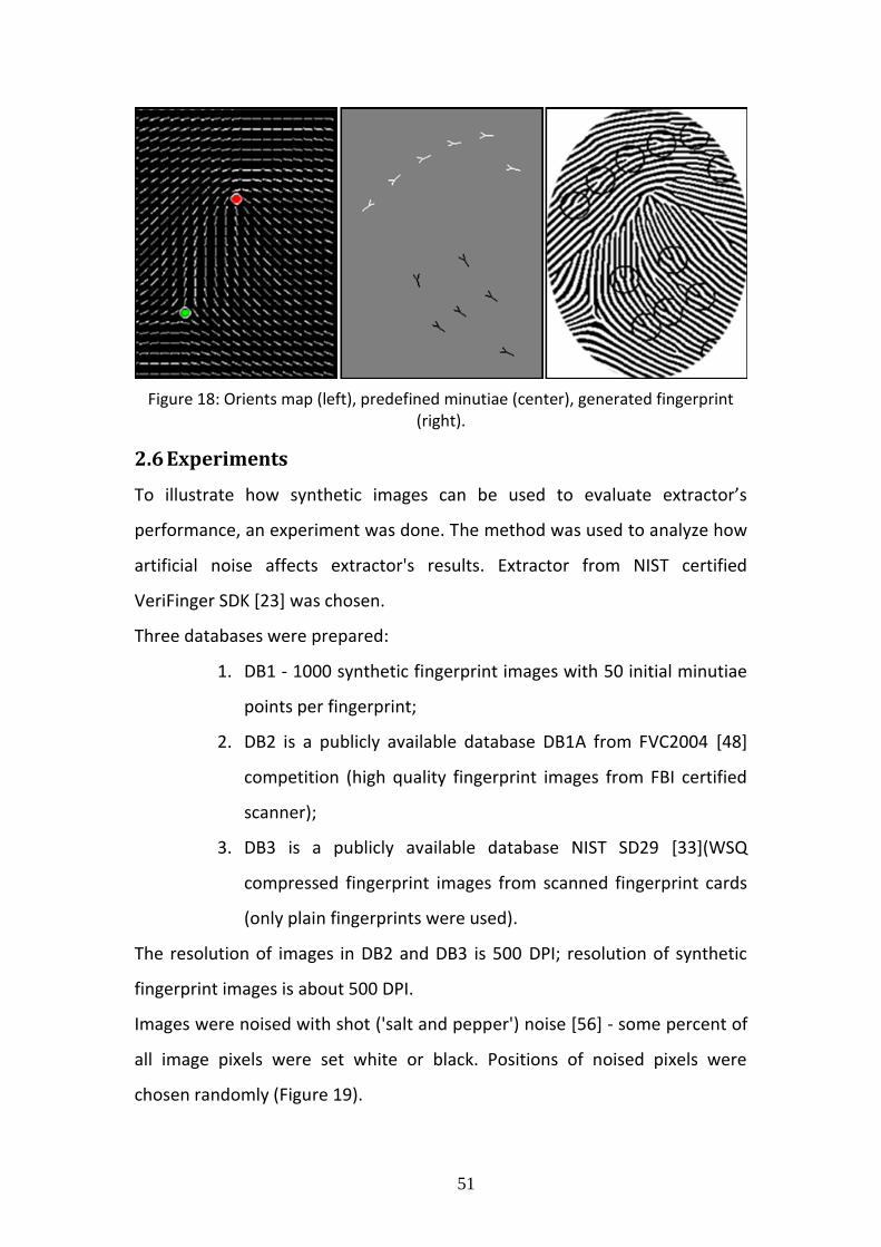
51

Figure 18: Orients map (left), predefined minutiae (center), generated fingerprint (right).

2.6 Experiments

To illustrate how synthetic images can be used to evaluate extractor’s

performance, an experiment was done. The method was used to analyze how

artificial noise affects extractor's results. Extractor from NIST certified

VeriFinger SDK [23] was chosen.

Three databases were prepared:

1. DB1 - 1000 synthetic fingerprint images with 50 initial minutiae

points per fingerprint;

2. DB2 is a publicly available database DB1A from FVC2004 [48]

competition (high quality fingerprint images from FBI certified

scanner);

3. DB3 is a publicly available database NIST SD29 [33](WSQ

compressed fingerprint images from scanned fingerprint cards

(only plain fingerprints were used).

The resolution of images in DB2 and DB3 is 500 DPI; resolution of synthetic

fingerprint images is about 500 DPI.

Images were noised with shot ('salt and pepper') noise [56] - some percent of

all image pixels were set white or black. Positions of noised pixels were

chosen randomly (Figure 19).

52

Figure 19: Examples of shot noise of different power on DB1 (left), DB2 (center), DB3 (right) (noise percentage: top left - 0%, right bottom – 80%).

Minutiae points from noised images were extracted and following statistics

for each noise density d (percentage of the noised pixels) from 0 to 100 were

calculated:

1. percent of initial minutiae points that was found on noised

image (Minutiae point was considered as found if it is the

nearest minutiae point to the initial minutiae point and the

distance to it is less than 10 pixels;

2. how found minutiae positions were affected by noise (the

average distance in pixels between initial minutiae and found

minutiae).

Since accurate minutiae positions on real databases are not known (as in

generated fingers), minutiae points extracted from not noised images were

considered as initial minutiae points. Results are presented in following

figures:

53

Figure 20: Quantity of initial minutiae points found on noised images (horizontal axis - noise density from 0% to 100%, vertical axis - quantity of found minutiae from 0

(0%) to 1 (100%).

Figure 21: Average distance between minutiae in noised image and minutiae in initial image (horizontal axis - noise density from 0% to 86%, vertical axis - average

distance in pixels.

0

0.1

0.2

0.3

0.4

0.5

0.6

0.7

0.8

0.9

1

1 8 15 22 29 36 43 50 57 64 71 78 85 92 99

DB1

DB2

DB3

0

0.5

1

1.5

2

2.5

3

3.5

1 5 9 13 17 21 25 29 33 37 41 45 49 53 57 61 65 69 73 77

DB1

DB2

DB3

54

It can be noticed from the Figure 20 that on DB1 more than 90% of minutiae

points are detected up to noise densities around 60% (when more than half of

image pixels are corrupted) and the average distance to initial minutiae point

is about 1.5 pixels (Figure 21).

On DB2 more than 90% of minutiae are detected if noise density is less than

20% (Figure 20), but the average distance to original minutiae point is still less

than one pixel (Figure 21).

On DB3 more than 90% of minutiae are detected only if noise density is less

than 5% (Figure21). At noise density 20% only 60% of minutiae are found and

the average distance to original minutiae point is more than one pixel (Figure

21).

Real fingerprint images have lower signal-to-noise ratio because some noise is

added during fingerprint acquisition process (dust on scanner, marks from

previously scanned fingerprints, digitization errors, image compression

artifacts).

We propose to use synthesized image database as references in estimation of

quality of the extractor. For example curve of Figure 20 that corresponds to

synthetic DB1 is the most right. We postulate that this curve corresponds for

ideal scanner or ideal database and has 100% quality. The measure of quality

can be defined as 100 * S1 / S1, where S1 is an area below the graph in Figure

20 that corresponds to DB1. Quality of DB2 and DB3 databases or their

corresponding scanners is 100 * S2 / S1 and 100* S2 / S1. Here S2 and S3 are

areas below the corresponding graphs in Figure 21. After calculation of the

areas, quantitative extractor quality on DB2 and DB3 was calculated. The

numbers are 64.7% for DB2 and 35.3% for DB3. Graphs in Figure 20 represent

proportion of reliable detected minutiae in respect of added “salt and

pepper” noise. Thus the calculated qualities represent extractor quality for

the two databases in the sense of quantity of reliably detected minutiae.

55

Graphs in Figure 21 can be used in the similar manner to estimate precision

of extracted minutiae positions. Average error on DB2 is 7.8 times higher than

on DB1, on DB3 – 11.1 times higher than on DB1. Note that in both cases

extraction qualities for DB3 were lower and this well correlates with published

ROC and DET characteristics for these databases [48], [58].

2.7 Summary and Conclusions of the Chapter

A method of fingerprint image generation was described in detail. The

method is fast, and can generate images with minutiae points that have

predefined properties such as location, direction and type. It can be used not

only to generate large databases of fingerprints, but to precisely evaluate

extraction algorithm performance and detect its weak sides (stability to noise,

scratches, deformations and other imperfections). Experiments show that

quality of generated images is much better than quality of real fingerprints

and since initial minutiae positions are known, the accuracy of evaluation is

higher.

It is common to evaluate database, extractor or matcher accuracy by

calculating statistics like ROC on some database, but the result of such

evaluation depends on all three components – quality of database, quality of

extractor and quality of matcher. When synthetic database is used, evaluation

results depend on only two components – quality of extractor and quality of

database. Influence of the matcher is eliminated by using synthetic database

as a reference. Two measures for extractor’s performance estimation on

different DB were introduced. The resulting quality is in the range of 0 and

100%, where 100% corresponds to the case of synthetic images. The obtained

numeric values of the qualities correspond to known ROC characteristics of

test databases.

The described method can be used to design an extraction algorithm that is

more tolerant to scanner noise, fingerprint scratches and deformations. Since

56

additional minutiae points appear in result image during generation process,

additional workaround may be needed to overcome this issue.

3 Fingerprint matching

3.1 Introduction

Most automatic fingerprint verification and identification systems use

minutiae information from fingerprints to align and compare images or their

templates to speed up the matching process. We refer to minutiae as ridge

ending or ridge bifurcation with any additional local features. Extraction of

minutiae from fingerprint image is out of the scope of this work.

Much effort has been made to create matching algorithms capable of dealing

with distortion and deformations in fingerprint images. Exhaustive overview

of possible methods is made in [20] and [21]. Thin-plate spline model is used

to deal with distortion in [5]: first, local matching is performed on structures

that consist of minutiae and its two closest neighboring minutiae points to

determine which minutiae possibly match, then global matching is made to

find registration parameters; after finding the global registration parameters

that coarsely align two fingerprints, elastic deformation is eliminated using

thin-plate spline model, and final match is made. The authors reported major

increase in performance. However, their approach uses registration

estimation that is not reliable when fingerprints are distorted since accurate

registration does not often exist, see Figure 22. Two distorted fingerprints are

presented. After registration, only small common part that is not distorted is

left.

57

Figure 22: Two different impressions of the same fingerprint before and after best registration.

Errors in registration lead to errors in further steps. Matching based on local

and global structures is described in [24]. Local matching uses local structures

that consist of minutiae point and its neighboring minutiae points and is

rotation and translation tolerant. Local structures from both fingerprints are

matched to find the best matching pair. This pair is used as a reference

correspondence point, and other minutiae points are aligned based on this

correspondence. After alignment global structure matching is performed. To

account for deformation, large bounding boxes are used, but to decrease the

probability of false match, the matching certainty level function that provides

some sort of match probability instead of just "matched" or "not matched"

result is defined. Although authors reported good matching performance, the

disadvantages of their matching algorithm are similar to [5]. If the fingerprints

are distorted, the exact registration parameters do not exist, and even the

reference local pair cannot be used to align them. Errors in choosing the right

reference point or incorrect alignment lead to incorrect match. Other

methods are described in literature [20], but most of them are either

variations of above described methods that use registration, or their

computational cost is too high or they use some other, not minutiae methods

to deal with distortion and cannot be used with existing fingerprint databases

based on minutiae. For example, an interesting method is introduced in [28]

where authors normalize the fingerprint image to a canonical form so that

ridges are equally spaced and less affected by distortion. In [7] a distortion

model that could describe elastic deformation found in fingerprint images is

58

presented. Authors validated it by manually setting deformation parameters,

but no automatic optimization technique that could be used to automatically

derive deformation parameters while matching minutiae is known. In general,

distortion elimination is a hard problem that could improve performance of

most matchers, if properly solved. After normalization or deformation

removal a rigid matcher could be used for direct comparison [18]. Another

normalization technique was introduced in [14] – the minutiae distance is

normalized at the matching stage according to the local ridge frequency. This

method could improve matcher performance for good quality fingerprints

where reliable frequency estimation is possible, and for minutiae pairs that

are not far from one another, so that changes in ridge frequency along the

fingerprint that occurs even in not distorted images are less than errors that

are made while estimating the frequency.

In this chapter, a completely new approach of minutiae matching is proposed

as a framework with broad range of possible implementations. One of the

most simple but effective implementation is discussed here. The method

consists of three main steps: matching of local structures, correspondence set

construction and validation of higher order local structures. The first step has

the following properties: Low false rejection ratio (FRR), rotation and

translation invariance, locality (for tolerance to deformations) and low

computational complexity.

Possible implementation will be discussed in section 3.3. The second step

receives a similarity matrix filled with similarity score of every minutiae point

from the first template compared with every minutiae point from the second

template. In spite of the fact, that one minutiae point from the first template

can be very similar to several different minutiae points from the second

template, every minutiae point can make only one correspondence between

the templates. Construction of minutiae correspondence set is discussed in

section 3.3.2. While constructing the minutiae correspondence set no

59

information about the global fingerprint structure is used. The last step of

global fingerprint structure validation is discussed in section 3.4.

3.2 Fingerprint Matching Without Global Alignment

This chapter is about a method of minutiae based fingerprint matching that is

robust to deformations and does not perform fingerprint alignment. It

concentrates on comparing rotation and translation invariant local structures

defined by minutiae point and its neighboring minutiae points. Then the

collection of most probable correspondences of matched minutiae is found.

Finally, the local structures of higher order are validated. All three steps are

completely rotation and translation invariant, robust to nonlinear

deformations and do not use any fingerprint alignment. Experimental results

on publicly available as well as internal databases showed an improved

performance of the proposed method in comparison with the traditional

minutiae based algorithms that perform fingerprint registration.

3.3 Local Matching

In most general case, template of fingerprint is the description of minutiae

points set. Two sets of minutiae must be compared while matching two

fingerprints. For simplicity, we will call (test set) – the first set of

minutiae and (sample set) – the second set of minutiae. The order of

sets is not important because the proposed method is symmetric. We define

local matching as a comparison of local structures from set to local

structures from set where every local structure is associated with minutiae

which serves as a reference point to that local structure. The result of local

matching step is a similarity matrix filled with similarities between

local structures.

3.3.1 Local Structure

Generally, local structure could be anything from a minutiae point identified

by a vector starting at and local ridge direction to a set of minutiae

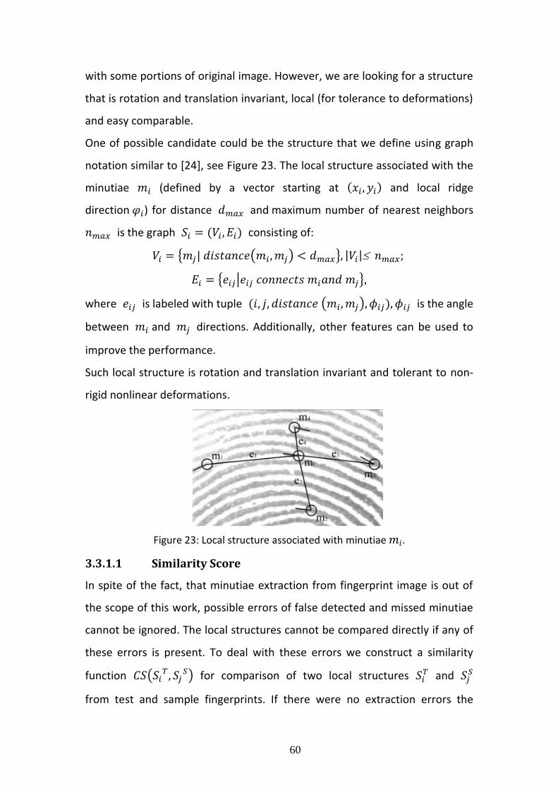
60

with some portions of original image. However, we are looking for a structure

that is rotation and translation invariant, local (for tolerance to deformations)

and easy comparable.

One of possible candidate could be the structure that we define using graph

notation similar to [24], see Figure 23. The local structure associated with the

minutiae (defined by a vector starting at and local ridge

direction ) for distance and maximum number of nearest neighbors

is the graph consisting of:

{ ( ) }

{ | },

where is labeled with tuple ( ) is the angle

between and directions. Additionally, other features can be used to

improve the performance.

Such local structure is rotation and translation invariant and tolerant to non-

rigid nonlinear deformations.

Figure 23: Local structure associated with minutiae .

3.3.1.1 Similarity Score

In spite of the fact, that minutiae extraction from fingerprint image is out of

the scope of this work, possible errors of false detected and missed minutiae

cannot be ignored. The local structures cannot be compared directly if any of

these errors is present. To deal with these errors we construct a similarity

function (

) for comparison of two local structures and

from test and sample fingerprints. If there were no extraction errors the

61

edges of every local structure could be sorted in clockwise (or

counterclockwise order) starting from the direction of associated minutiae

and compared directly by a function:

(

) ∑

| |

(3.1)

(

) {

(3.2)

| (

) (

)|,

| | | | ,

– thresholds, – predefined parameters.

However, we can deal with errors introduced by extraction in the following

way:

1. Sort edges in a clockwise order (starting from the direction

of associated minutiae) into a sequence ;

2. Sort edges in a clockwise order (starting from the direction

of associated minutiae) into a sequence ;

3. Find the longest common subsequence (LCS) of and

using the same similarity function CE from (3.2) for comparison

of sequence elements.

4. Sum up the similarities of edges that make the longest common

subsequence:

(

) ∑ (

)

(

)

(3.3)

As a convenient abuse of terminology we will use instead of to

represent similarity between two local structures.

3.3.2 Correspondence Set Construction

After calculating similarity between every local structure from test and

sample fingerprints similarity matrix is filled with these values. This

62

matrix can be used to construct a correspondence set of minutiae pairs where

every local structure belongs maximum to one correspondence:

{(

)|

} (3.4)

Though many different approaches can be used to find minutiae

correspondence set, a maximum weighted matching on bipartite graphs is

used to find the correspondence set maximizing the sum of similarities

between local structures.

Bipartite graph is constructed from similarity matrix with vertices defined by

local structures from both fingerprints and weighted edges defined by greater

than 0 similarities between associated local structures. We use Hungarian

algorithm [59] to solve this problem in time in worst case.

3.4 Validation

Until a correspondence set is constructed no global fingerprint registration is

used and for robustness to deformations it will not be used anywhere in the

proposed method. Although local structures from test and sample fingerprints

can have high similarity they can be located differently in respect to each

other in fingerprints (see Figure 24).

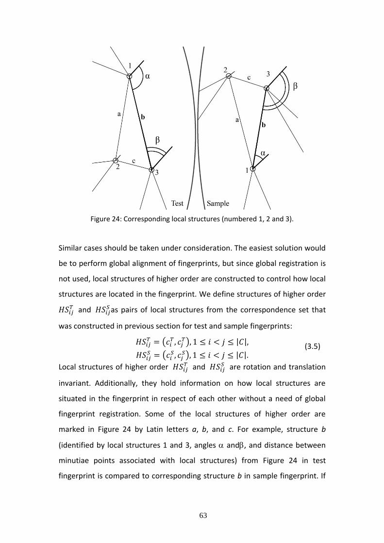
63

Figure 24: Corresponding local structures (numbered 1, 2 and 3).

Similar cases should be taken under consideration. The easiest solution would

be to perform global alignment of fingerprints, but since global registration is

not used, local structures of higher order are constructed to control how local

structures are located in the fingerprint. We define structures of higher order

and

as pairs of local structures from the correspondence set that

was constructed in previous section for test and sample fingerprints:

(

)

(

)

(3.5)

Local structures of higher order and

are rotation and translation

invariant. Additionally, they hold information on how local structures are

situated in the fingerprint in respect of each other without a need of global

fingerprint registration. Some of the local structures of higher order are

marked in Figure 24 by Latin letters a, b, and c. For example, structure b

(identified by local structures 1 and 3, angles and, and distance between

minutiae points associated with local structures) from Figure 24 in test

fingerprint is compared to corresponding structure b in sample fingerprint. If

64

the structures are not consistent they are not used in calculating similarity

score between fingerprints.

3.4.1.1 Similarity Score

We define similarity score SS between two local structures of higher order

and

as:

(

)

{

(3.6)

minutiae points associated with local structures from

| (

) (

)|

,

– angles between the segments connecting the local structures

of higher order and directions of their associated minutiae,

– predefined parameters.

3.5 Final Similarity Score

We define similarity score between two fingerprints as a sum of similarity

scores between all local structures of higher order (that passed a validation

step) combined with similarity scores of local structures that make them:

∑ (

)

(3.7)

where

,

are local structures that make and

,

( (

)

(

)) can be one of the following (but

not limited to):

(

)

(

(

)); (3.8)

65

(

)

(

) (3.9)

(

) √

. (3.10)

function is used to normalize similarity score for differently sized

fingerprints.

Selection of the most suitable and functions can improve matching

performance in cases when fingerprints of different sizes are compared.

and were used in this work together

with (3.9) equation.

3.6 Evaluation of threshold parameters

3.6.1 Threshold Parameters in Local Structures

Two threshold parameters are used in constructing local structures:

and . Experimental results show that changing value of parameter

hardly changes matching performance. However, to make structures

more local the value of pixels was chosen. Additional testing was

performed on several databases for choosing the value of parameter.

It showed that is a tradeoff between speed and quality. The value of 10

was chosen. The results are shown in Figure 25.

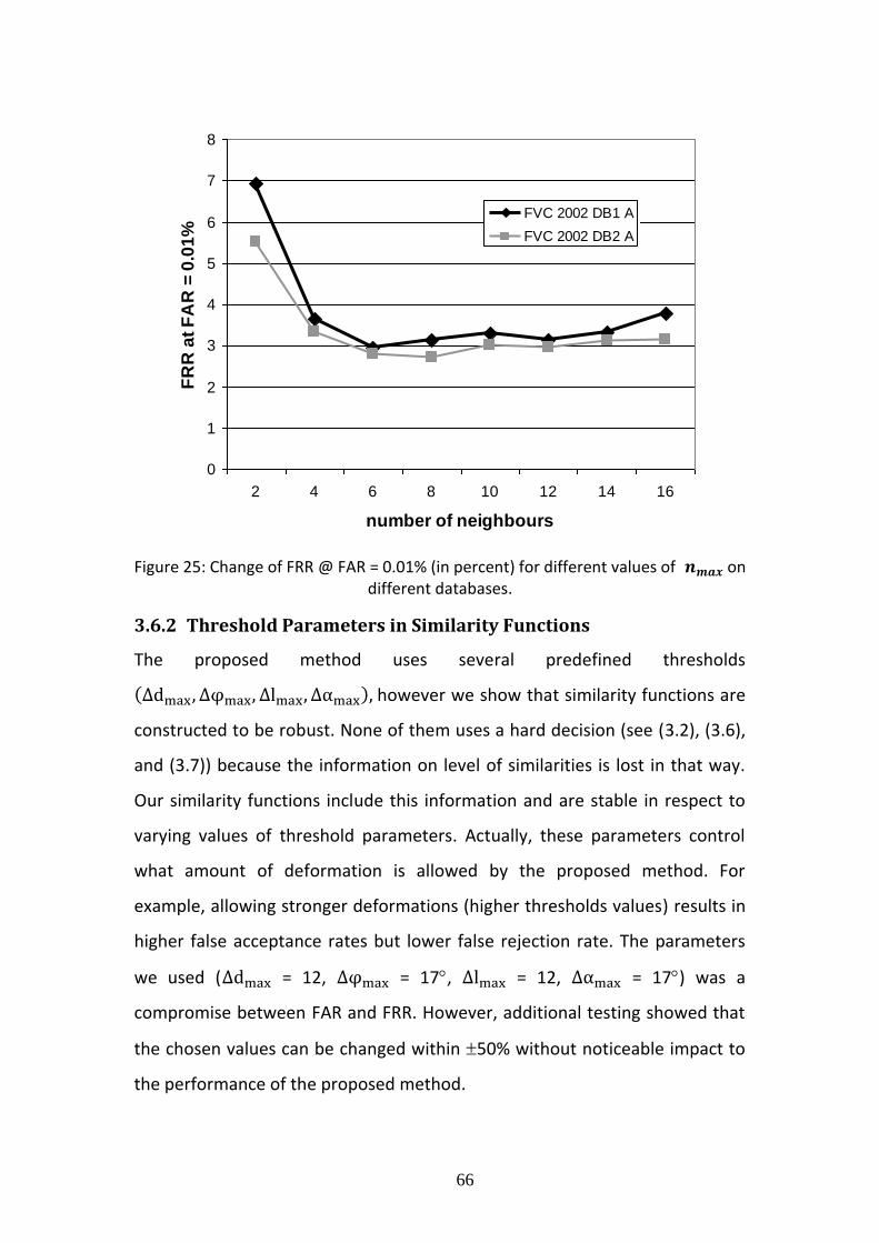
66

Figure 25: Change of FRR @ FAR = 0.01% (in percent) for different values of on different databases.

3.6.2 Threshold Parameters in Similarity Functions

The proposed method uses several predefined thresholds

however we show that similarity functions are

constructed to be robust. None of them uses a hard decision (see (3.2), (3.6),

and (3.7)) because the information on level of similarities is lost in that way.

Our similarity functions include this information and are stable in respect to

varying values of threshold parameters. Actually, these parameters control

what amount of deformation is allowed by the proposed method. For

example, allowing stronger deformations (higher thresholds values) results in

higher false acceptance rates but lower false rejection rate. The parameters

we used ( = 12, = 17, = 12, = 17) was a

compromise between FAR and FRR. However, additional testing showed that

the chosen values can be changed within 50% without noticeable impact to

the performance of the proposed method.

0

1

2

3

4

5

6

7

8

2 4 6 8 10 12 14 16

number of neighbours

FR

R a

t F

AR

= 0

.01

%

FVC 2002 DB1 A

FVC 2002 DB2 A

67

3.7 Performance Evaluation

The complexity of the algorithm consists of three man stages: local structure

matching, correspondence set construction and validation. The complexities

of the stages when number of features in first fingerprint is and in the

second fingerprint is are:

respectively, that gives resulting complexity of the algorithm:

.

The performance of the proposed method was tested on publicly available

NIST Special Database 29 [33] fingerprint database (hereafter referred as

SD29). The database consists of 216 ten-print fingerprint card pairs with both

the rolled and plains scanned at 19.7 pixels per mm. For direct comparison we

chose publicly available NIST fingerprint image software NFIS2 [34] minutiae

based fingerprint matching algorithm (hereafter referred as BOZORTH3).

Fingerprint minutiae extractor from NFIS2 (MINDTCT) was not used in the

evaluation because of big number of false minutiae it produces (BOZORTH3

matcher uses only 150 minutiae of best quality from the fingerprint template

to deal with this problem). We tested the proposed matching method with

commercially available fingerprint minutiae extraction algorithm of better

quality [23] (hereafter referred as COMM). We will refer to the proposed

method as Local Structure Matcher (LSM) in all experiments.

SD29 database consists only of fingerprint images that were scanned from

fingerprint cards. Additional tests were done to prove that the proposed

method works well with live scanned fingerprints. The following databases

were chosen:

1. DB1 from FVC2002 fingerprint verification competition [18]

collected with optical sensor "TouchView II" from Identix. The

database consists of 800 different fingerprints with 8

impressions per finger;

68

2. DB2 from FVC2002 fingerprint verification competition collected

with optical sensor optical sensor "FX2000" from Biometrika.

The database consists of 800 different fingerprints with 8

impressions per finger;

3. Neurotechnology’s internal database collected with optical

single-finger scanner "DFR 2090" from Identix (hereafter

referred as INTERNAL1). The database consists of 1400 different

fingerprints with 10 impressions per finger;

4. Neurotechnology’s internal database collected with high-quality

optical single-finger scanner "Cross Match Verifier 300"

(hereafter referred as INTERNAL2) recommended for large scale

automatic fingerprint identification systems. The database

consists of 1 400 different fingerprints with 10 impressions per

finger.

5. A relative comparison with other algorithms that perform

registration can be found at: http://bias.csr.unibo.it/fvc2006/

3.8 Results

NIST VTB fingerprint system with Bozorth98 matcher (previous version of

BOZORTH3) participated in Fingerprint Vendor Technology Evaluation (FpVTE)

2003 [36] and proved to be comparable to other commercial algorithms and

even better than almost half of the contestants. The following experiment

shows an improvement of the proposed method over BOZORTH3 matcher

with COMM minutiae extractor. 18 ROC curves were calculated on different

parts of SD29 [35] (P2P – plain vs. plain fingers, P2R – plain vs. rolled fingers,

R2R – rolled vs. rolled fingers, RT – right thumb, LT – left thumb, RI – right

index, LI – left index, RM – right middle, LM – left middle) of SD29 for both

methods. The results (False rejection rate – FRR when false acceptance rate –

FAR is 0.01%) are shown in Table 3 and

Table 4.

69

Table 3: COMM+BOZORTH3 FRR @ FAR = 0.01% on different parts of SD29

part RT LT RI LI RM LM average

P2P 7.1 6.2 18.9 15.0 14.8 14.1 12.68

P2R 12.7 12.8 14.7 18.6 14.6 12.2 14.27

R2R 16.3 11.3 6.6 5.9 8.3 6.0 9.08

Table 4: COMM+ LSM FRR @ FAR = 0.01% on different parts of SD29.

part RT LT RI LI RM LM average

P2P 7.14 9.89 14.8 11.5 15.9 13.2 12.07

P2R 5.36 9.34 9.07 12.5 9.62 9.34 9.205

R2R 4.95 7.69 4.4 6.59 5.49 8.79 6.318

The proposed method improves FRR at FAR = 0.01% from 12.01% to 9.20% on

average. As expected, the largest improvement was gained on rolled-to-rolled

fingerprint matching were stronger deformations of fingerprints are possible.

Figure 26 and Figure 27

Figure show the performance of the proposed method on live scan

fingerprints from FVC2002 databases that were collected with optical

scanners.

Figure 26: COMM+BOZORTH3 compared to COMM+LSM on FVC2002 DB1 database.

70

Figure 27: COMM+BOZORTH3 compared to COMM+LSM on FVC2002 DB2 database.

Summary of improvements (FRR @ FAR = 0.01%) over all databases is

presented in Table 5.

Table 5: FRR @ FAR = 0.01% on tested databases with commercial minutiae extractor

database BOZORTH3 LSM

SD29 (average) 12.01 9.20

FVC2002 DB1 8.73 3.29

FVC2002 DB2 5.82 3.00

INTERNAL1 5.65 2.3

INTERNAL2 1.78 0.44

The largest improvement was achieved for the live scanned fingerprints.

False rejection rate (FRR) at 0.01% FAR is up to 4 times (one-tailed paired t-

test; p < 0.0005; Table 5) lower comparing with BOZORTH3 matcher.

3.9 Summary and Conclusions of the Chapter

A framework to match deformed fingerprints was presented in this chapter. It

consists of simple and intuitive steps. The proposed implementation of the

steps is straightforward and flexible, does not use registration, and is capable

of matching deformed fingerprints. It leaves much freedom in combining the

suggested methods with other approaches. Evaluation of algorithm was made

71

on large data sets with different matching parameters. It has been shown that

proposed method is flexible and tolerant to rotation, translation and

deformation of fingerprint images. Performance of the method was compared

with BOZORTH3 matcher and improvements up to 4 times (one-tailed paired

t-test; p < 0.0005; Table 5) in false rejection rates at 0.01% FAR were

demonstrated.

4 Speaker Recognition

4.1 Introduction

New text independent speaker identification method is presented. In this

chapter. Phase spectrum of all-pole linear prediction (LP) model is used to

derive the speech features. The features are represented by pairs of numbers

that are calculated from group delay extremums of LP model spectrum. The

first component of the pair is an argument of maximum of group delay of all

pole LP model spectrum and the second is an estimation of spectrum

bandwidth at the point of spectrum extremum. A similarity metric that uses

group delay features is introduced. The metric is adapted for text

independent speaker identification with general assumption that test speech

channel may contain multiple speakers. It is demonstrated that automatic

speaker recognition system with proposed features and similarity metric

outperforms systems based on Gaussian mixture model with Mel frequency

cepstral coefficients, formants, antiformants and pitch features.

Automatic speaker recognition quality still remains pretty low in comparison

with other biometric identification methods based on fingerprints [13], irises

and even faces analysis [26] [30]. Conventionally, the front-end of the

recognition system uses features such as cepstral, Bark or Mel frequency

cepstral coefficients [4]. The features are based on spectrum amplitude of the

speech frames or their residual parts of linear prediction model [16][15]. In

72

our opinion mainstream of speaker recognition algorithms underestimate

information contained in phase spectrum. The idea that spectrum phase can

contain valuable information for speaker recognition is not very surprising

because it is known that traditional power spectrum resonant characteristics

can be derived exclusively from the phase spectrum [11], [22]. To resolve

stability problem, the phase spectrum of traditional Linear Prediction (LP)

model is used. In [32]the group delay features for speaker recognition were

derived directly from the Fourier spectrum of the speech frames. Such

approach requires special techniques dealing with instabilities of unwarped

Fourier spectrum. We combine [11] and [37] techniques to extract group

delay features of LP model. In [11] third order derivatives of the LPC phase

spectrum were used to extract speech formants. We explore only first and

second derivatives of LPC phase spectrum. The zero-crossings of the second

derivative provides information about formants positions. LPC phase first

derivative at formants frequencies gives simple approximations of the

formants bandwidth. In [37] a connection between LPC phase and Line

Spectrum Frequencies (LSF) is described. That inspired us to construct a

symmetrized form of LPC phase representation which saves features

computation cost and gives simple formulas for approximation of LPC

spectrum poles. Gaussian Mixture Model (GMM) (see[25], [11]) becomes a

standard technique for modeling of distributions of speakers features and

their comparison. Since our features are restricted to the rectangle

(0,1))(0, we estimated features distribution using histogram technique

and constructed an information theory based similarity measure for

comparison of speech utterances.

73

4.2 Group Delay Features of all-pole LP model

4.2.1 Linear Prediction

In Linear prediction (LP) model [10] samples of a speech frame are

represented in the form

∑

(4.1)

where are the Linear Prediction Coefficients (LPCs), is the

model order, and are the excitation gain and source, respectively. The

LPCs are derived adaptively for each 20-30 ms speech frame by minimization

of excitation mean square energy. For simplicity, we will assume that the

order of LP model is uneven, i.e. . The LPC spectrum or the

transfer function of the LP filtering is defined by:

(4.2)

where ∑

(4.3)

is the inverse filter. The LPC spectrum represents an envelope of the speech

spectrum.

4.2.2 Phase of Spectrum of LP model

Let us define symmetrical polynomial and antisymmetrical polynomial

by the formulas:

(4.4)

√ (4.5)

The and polynomials are related to the symmetrical polynomial

and of Line Spectrum Frequencies (LSF) analysis [37] by the

following formulas:

74

(4.6)

(4.7)

On the unit circle are real-valued,

(4.8)

and (4.9)

The equations (4.8) and (4.9) show that the frequency response and the

phase of the transfer function of the LP model satisfy the equations:

√ (4.10)

and ( ( )

( ))

√ .

(4.11)

4.2.3 LPC Phase Spectrum Features

The LPC spectrum in the all-pole representation has the following form:

∏

(4.12)

where is location of the m-th pole of the LPC spectrum, and

is the angular frequency of the pole. From Eq. (4.12) follows that

the mth pole contributes to the LPC phase spectrum with the additive term

).

Therefore for the first and second phase spectrum derivative we have:

∑

(4.13)

∑

(4.14)

The negative derivative of phase of the LP spectrum is called group delay of LP

model. The poles locations are not estimated and the phase spectrum

75

derivatives are calculated by numerical differentiation of Eq. (4.11) identity to

reduce calculation time.

Equation (4.13) gives that for the strong pole with close to 1 one can

expect local maximum of the group delay at a point close to the angular

frequency . The local maximum m can be found as second derivative

zero-crossing point which is closest to the . (4.13) gives:

(4.15)

and

(4.16)

Considering the provided observations, we define the group delay features of

a speech frame as a set of pairs

(

) (4.17)

where is the set of all zero crossings of the phase spectrum second

derivative that belong to the radian frequency interval and

(4.18)

defines a bandwidth of a formant of the speech frame.

4.3 Speech Utterance Similarity Measure for Speaker

Identification

Suppose there are two sampled speech utterances and and

similarity between them must be measured. Let's assume that samples

belong to a speaker of the training set and samples belong to a

speech utterance of one, two or even more test speakers. The similarity

measure should estimate the probability that speaker of the training set

speaks in speech utterances. Such speaker recognition scenario occurs in

forensic evaluation of the evidence using automatic speaker recognition

systems. In forensic evaluation speech utterance of a training speaker can be

recorded in a separate channel or manually segmented from multi speakers

76

speech utterances, and test speech utterances may consists of natural records

of persons under investigation.

4.3.1 Features statistics.

In previous section we introduced LPC phase spectrum variation features

which for the k-th speech frame consist of

pairs where is the

frequency position of the m-th local maximum of the group delay and a

bandwidth of the extremum point. The speech utterances are divided into

short time intervals of 1 sec. Duration and distribution of the group delay

features of their frames is estimated. Since distance between two neighbor

frames is sec., we have about pairs

of features

in 1 sec. duration utterance. Distribution of

is

estimated by division of

into rectangular boxes and

calculating number of pairs

that belong to the boxes. Warping

parameter is adapted to sampling frequency so that division

of frequency range

in equal width intervals corresponds roughly to

the Bark frequency scale. Possible bandwidth interval is divided into

increasing width intervals of total number .

4.3.2 Similarity measure of two short speech utterances

Similarity measure between two speech utterances is defined as a mutual

information of the two group delay feature distributions. Let is

total number of all possible rectangular boxes and

and

are feature vectors which components are numbers of

group delay features belonging to boxes . By definition, all the and

correspond to and seconds time intervals of and

speech utterances respectively. Let and

are Shannon's entropies of

the and

counts, i. e.,

77

∑

(4.19)

∑

(4.20)

∑

∑

(4.21)

Let

denotes conjoint counts of

and

and

∑

(4.22)

is the Shannon's entropy of the

. It is easy to prove the following

statement about a relation between the three entropies.

Theorem 1. For any counts and

and their conjoint count

the

following inequalities hold true:

(4.23)

where

(4.24)

and (4.25)

Proof. The Gibbs' inequality [17] for any two distributions and gives

∑

∑

Applying this inequality for

or

and

we have

∑

∑

|

| (

| |

) ∑

that proves the left hand side inequality of Eq. (4.23).

78

The right hand side inequality of Eq. (4.23) can be justified by information

theory reasoning.

is the average Shannon's information for appearance

of a text letter of the text with

letters counts. The information about a

letter of the text with conjoint

counts can be obtained using the

following procedure. At first the question is asked "is this letter from the text

with or

counts"? Then, depending on the answer to the first

question, the second question is asked "which letter is from the text with

counts?" or "which letter is from the text with

counts?" with probability

and respectively. Answer to the first question contains

bits of information and the second one contains

or

bits of information with probability and respectively. Since

the strategy of provided two questions is not optimal in general, we have the

right hand side inequality of Eq. (4.23).

To provide a formal proof of the right hand side inequality of Eq. (4.23) let us

consider continuous function:

It is easy to check that this function is subadditive, that is

Really, if is fixed then

( )

(

)

and

Therefore . Applying this inequality we

have:

∑ (

| |

| |) (

| |

| |)

∑

| | (

| |

)

∑

| | (

|

|)

.

79

Definition 1. Similarity of of time interval (in seconds) of

speech utterance of the speaker to the time interval of the

speaker(s) is the number

(4.26)

Theorem 1 gives that the similarity of any two speech utterances

and is always non-negative and not greater than 1 . The next

definition gives similarity of short speech utterance to all the

utterances.

Definition 2. Similarity of short speech utterance to the

utterances is the number

( ) ∑ ( )

, (4.27)

where is the amount of seconds in speech utterance. In other words,

similarity is the average similarity of utterance to the

set of all of one second duration utterances .

The last definition combines short segments similarities to an integrated

similarity of and utterances.

Definition 3. Similarity of speech utterances to the utterances is the

number

( ) (4.28)

The provided similarity measure is asymmetrical (in general

). This is explained by the asymmetry in and data:

consists of utterances of one speaker and may contain utterances of two

or even more speakers. If a priori contains speech utterances of only one

speaker too, the can be modified to symmetrical similarity by

skipping "half biggest" words in Definition 3. All provided speech similarity

80

measures are based on mutual information, are non-negative, and do not

exceed 1. If and are totally different, i.e. the and group delay

features points belong to non intersecting sets of boxes , then, with all

and ,

and . In the opposite case,

when the all counts are proportional (

)

and . Consequently, the similarity measure

has a probabilistic interpretation: is a probability that speaker

participates in dialogue.

4.4 Experimental Results

4.4.1 Preprocessing of initial data

The following standard steps of initial data preprocessing were used in all our

experimentations: Silent or low energy speech intervals were detected and

removed from the further analysis, sound data was pre-emphasized with first

order filter of the form . speech utterance was segmented into

msec. frames with msec. overlapping, frame samples were windowed

with Hanning window, first order all-pass filter with warping parameter

[29] was applied to the windowed speech data.

4.4.2 A graphical illustration of group delay features

A speech frame with LPC log power spectrum represented Figure 28

illustrates ideas about group delay features. The first derivative of LPC phase

spectrum of the same speech frame is presented in Figure 29. Comparing LPC

log power spectrum and LPC phase spectrum variation, one can notice that

the last has two additional formants (maximums of the spectrum). The rest

five formants of both spectrums have similar positions at frequency axis,

however, peaks of the first derivative of LPC phase spectrum are more

prominent than that of LPC log power spectrum.

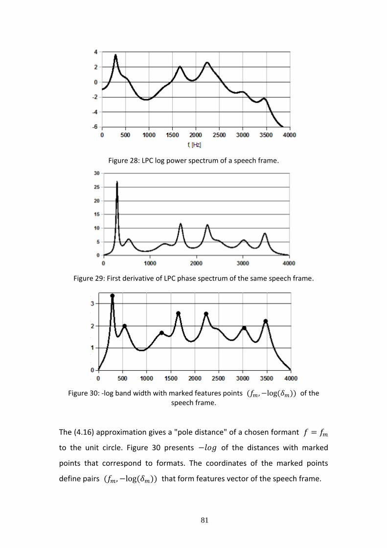
81

Figure 28: LPC log power spectrum of a speech frame.

Figure 29: First derivative of LPC phase spectrum of the same speech frame.

Figure 30: -log band width with marked features points of the speech frame.

The (4.16) approximation gives a "pole distance" of a chosen formant

to the unit circle. Figure 30 presents of the distances with marked

points that correspond to formats. The coordinates of the marked points

define pairs that form features vector of the speech frame.

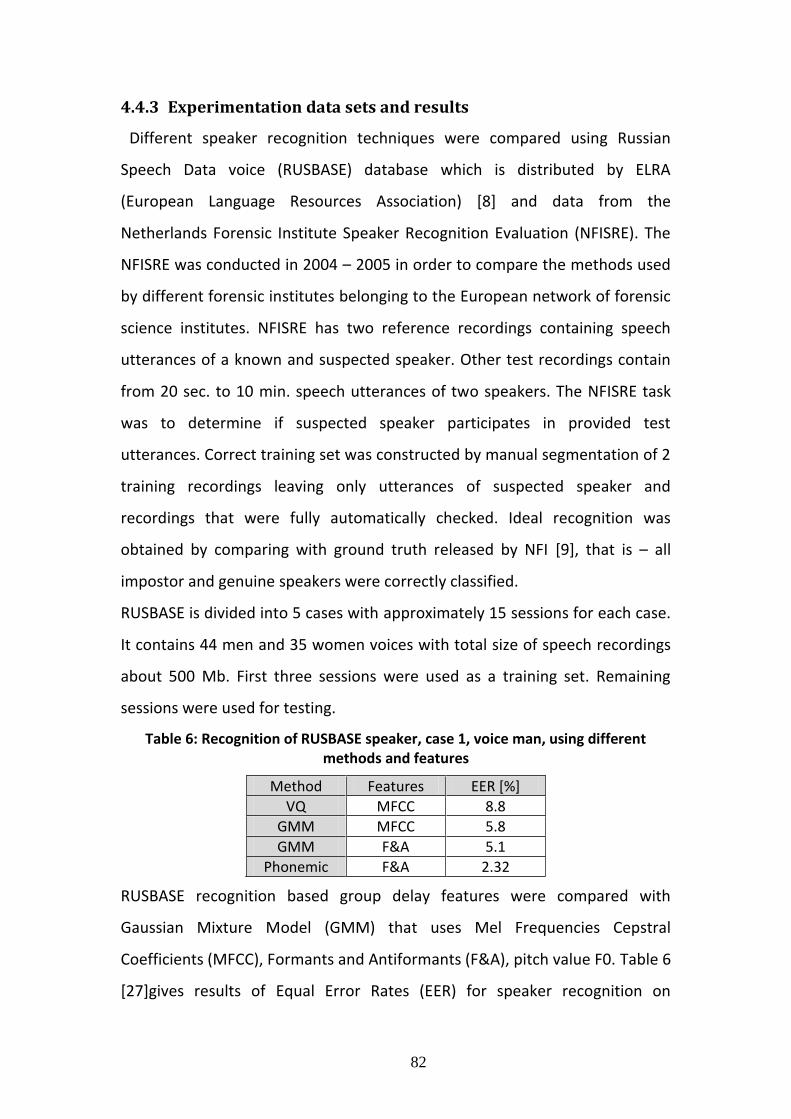
82

4.4.3 Experimentation data sets and results

Different speaker recognition techniques were compared using Russian

Speech Data voice (RUSBASE) database which is distributed by ELRA

(European Language Resources Association) [8] and data from the

Netherlands Forensic Institute Speaker Recognition Evaluation (NFISRE). The

NFISRE was conducted in 2004 – 2005 in order to compare the methods used

by different forensic institutes belonging to the European network of forensic

science institutes. NFISRE has two reference recordings containing speech

utterances of a known and suspected speaker. Other test recordings contain

from 20 sec. to 10 min. speech utterances of two speakers. The NFISRE task

was to determine if suspected speaker participates in provided test

utterances. Correct training set was constructed by manual segmentation of 2

training recordings leaving only utterances of suspected speaker and

recordings that were fully automatically checked. Ideal recognition was

obtained by comparing with ground truth released by NFI [9], that is – all

impostor and genuine speakers were correctly classified.

RUSBASE is divided into 5 cases with approximately 15 sessions for each case.

It contains 44 men and 35 women voices with total size of speech recordings

about 500 Mb. First three sessions were used as a training set. Remaining

sessions were used for testing.

Table 6: Recognition of RUSBASE speaker, case 1, voice man, using different methods and features

Method Features EER [%]

VQ MFCC 8.8

GMM MFCC 5.8

GMM F&A 5.1

Phonemic F&A 2.32

RUSBASE recognition based group delay features were compared with

Gaussian Mixture Model (GMM) that uses Mel Frequencies Cepstral

Coefficients (MFCC), Formants and Antiformants (F&A), pitch value F0. Table 6

[27]gives results of Equal Error Rates (EER) for speaker recognition on

83

RUSBASE, case 1, men voices, using MFCC, F&A, and F0 features and Vector

Quantization (VQ) (see [15]) and GMM recognition methods. The EER ranges

from 2.32% to 8.8 % (see Table 6). On the group delay and mutual information

based speaker recognition algorithm for the same data gives EER = 0.042%.

Table 7 provides full results of speaker recognition of RUSBASE. Here Zero FAR

is false acceptance rate (FAR) when false rejection rate (FRR) is 0% and Zero

FRR is False rejection rate (FRR) when false acceptance rate (FAR) is 0%.

Table 7: Speaker recognition using phase spectrum features and of mutual information type similarity. RUSBASE data set, case 1 – 5

Case Voice Zero FAR[%] EER[%] Zero FRR[%]

1 man 1.8 0.042 0.12

1 woman 1.96 0.042 0.07

2 man 0.8 0.084 0.12

2 woman 2.17 0.2 1.37

3 man 3.19 0.058 0.09

3 woman 1.96 0.033 0.06

4 man 0.6 0.01 0.02

4 woman 4.6 0.112 0.15

5 man 2.79 0.199 0.59

5 woman 0.44 0.007 0.01

The new speaker recognition technique showed a reduction of equal error

rate up to twenty times in comparison to traditional methods that use

features derived exclusively from the amplitude of the power spectrum.

4.5 Summary and Conclusions of the Chapter

It is shown that phase of transfer function defined by linear prediction model

can be used for derivation of features of utterances. The features represent

extremes of the group delay of the LP model. Similarity measure between two

speech utterances was defined as mutual information of the two group delay

feature distributions. The performance of group delay features and their

similarity metric was tested on two speaker datasets that contain text-

dependent and text-independent utterances. The new speaker recognition

technique showed up a reduction of equal error rate up to twenty times in

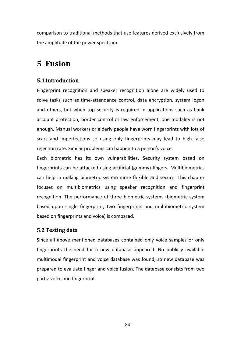
84

comparison to traditional methods that use features derived exclusively from

the amplitude of the power spectrum.

5 Fusion

5.1 Introduction

Fingerprint recognition and speaker recognition alone are widely used to

solve tasks such as time-attendance control, data encryption, system logon

and others, but when top security is required in applications such as bank

account protection, border control or law enforcement, one modality is not

enough. Manual workers or elderly people have worn fingerprints with lots of

scars and imperfections so using only fingerprints may lead to high false

rejection rate. Similar problems can happen to a person’s voice.

Each biometric has its own vulnerabilities. Security system based on

fingerprints can be attacked using artificial (gummy) fingers. Multibiometrics

can help in making biometric system more flexible and secure. This chapter

focuses on multibiometrics using speaker recognition and fingerprint

recognition. The performance of three biometric systems (biometric system

based upon single fingerprint, two fingerprints and multibiometric system

based on fingerprints and voice) is compared.

5.2 Testing data

Since all above mentioned databases contained only voice samples or only

fingerprints the need for a new database appeared. No publicly available

multimodal fingerprint and voice database was found, so new database was

prepared to evaluate finger and voice fusion. The database consists from two

parts: voice and fingerprint.

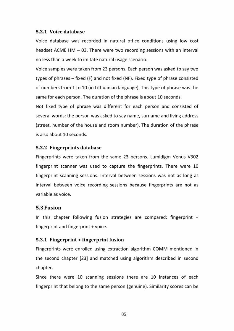
85

5.2.1 Voice database

Voice database was recorded in natural office conditions using low cost

headset ACME HM – 03. There were two recording sessions with an interval

no less than a week to imitate natural usage scenario.

Voice samples were taken from 23 persons. Each person was asked to say two

types of phrases – fixed (F) and not fixed (NF). Fixed type of phrase consisted

of numbers from 1 to 10 (in Lithuanian language). This type of phrase was the

same for each person. The duration of the phrase is about 10 seconds.

Not fixed type of phrase was different for each person and consisted of

several words: the person was asked to say name, surname and living address

(street, number of the house and room number). The duration of the phrase

is also about 10 seconds.

5.2.2 Fingerprints database

Fingerprints were taken from the same 23 persons. Lumidigm Venus V302

fingerprint scanner was used to capture the fingerprints. There were 10

fingerprint scanning sessions. Interval between sessions was not as long as

interval between voice recording sessions because fingerprints are not as

variable as voice.

5.3 Fusion

In this chapter following fusion strategies are compared: fingerprint +

fingerprint and fingerprint + voice.

5.3.1 Fingerprint + fingerprint fusion

Fingerprints were enrolled using extraction algorithm COMM mentioned in

the second chapter [23] and matched using algorithm described in second

chapter.

Since there were 10 scanning sessions there are 10 instances of each

fingerprint that belong to the same person (genuine). Similarity scores can be

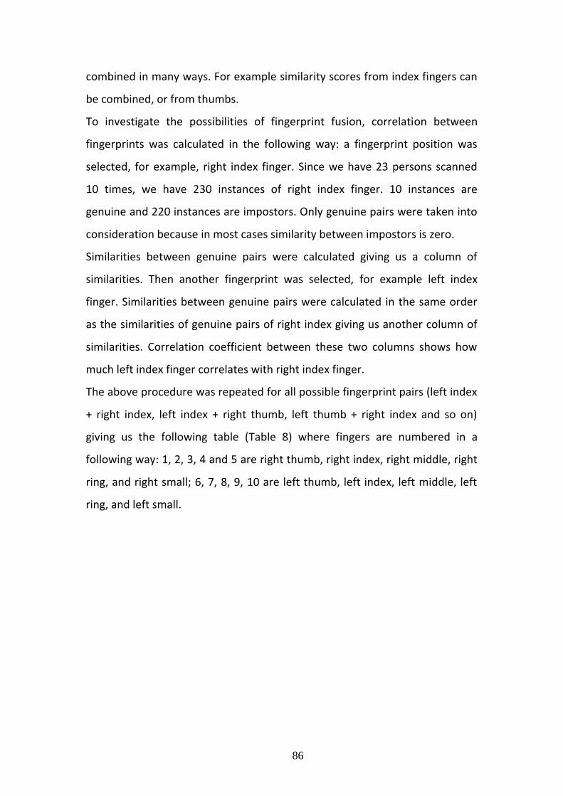
86

combined in many ways. For example similarity scores from index fingers can

be combined, or from thumbs.

To investigate the possibilities of fingerprint fusion, correlation between

fingerprints was calculated in the following way: a fingerprint position was

selected, for example, right index finger. Since we have 23 persons scanned

10 times, we have 230 instances of right index finger. 10 instances are

genuine and 220 instances are impostors. Only genuine pairs were taken into

consideration because in most cases similarity between impostors is zero.

Similarities between genuine pairs were calculated giving us a column of

similarities. Then another fingerprint was selected, for example left index

finger. Similarities between genuine pairs were calculated in the same order

as the similarities of genuine pairs of right index giving us another column of

similarities. Correlation coefficient between these two columns shows how

much left index finger correlates with right index finger.

The above procedure was repeated for all possible fingerprint pairs (left index

+ right index, left index + right thumb, left thumb + right index and so on)

giving us the following table (Table 8) where fingers are numbered in a

following way: 1, 2, 3, 4 and 5 are right thumb, right index, right middle, right

ring, and right small; 6, 7, 8, 9, 10 are left thumb, left index, left middle, left

ring, and left small.

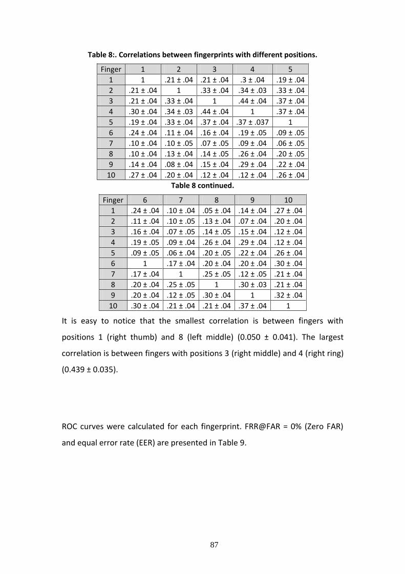
87

Table 8:. Correlations between fingerprints with different positions.

Finger 1 2 3 4 5

1 1 .21 ± .04 .21 ± .04 .3 ± .04 .19 ± .04

2 .21 ± .04 1 .33 ± .04 .34 ± .03 .33 ± .04

3 .21 ± .04 .33 ± .04 1 .44 ± .04 .37 ± .04

4 .30 ± .04 .34 ± .03 .44 ± .04 1 .37 ± .04

5 .19 ± .04 .33 ± .04 .37 ± .04 .37 ± .037 1

6 .24 ± .04 .11 ± .04 .16 ± .04 .19 ± .05 .09 ± .05

7 .10 ± .04 .10 ± .05 .07 ± .05 .09 ± .04 .06 ± .05

8 .10 ± .04 .13 ± .04 .14 ± .05 .26 ± .04 .20 ± .05

9 .14 ± .04 .08 ± .04 .15 ± .04 .29 ± .04 .22 ± .04

10 .27 ± .04 .20 ± .04 .12 ± .04 .12 ± .04 .26 ± .04

Table 8 continued.

Finger 6 7 8 9 10

1 .24 ± .04 .10 ± .04 .05 ± .04 .14 ± .04 .27 ± .04

2 .11 ± .04 .10 ± .05 .13 ± .04 .07 ± .04 .20 ± .04

3 .16 ± .04 .07 ± .05 .14 ± .05 .15 ± .04 .12 ± .04

4 .19 ± .05 .09 ± .04 .26 ± .04 .29 ± .04 .12 ± .04

5 .09 ± .05 .06 ± .04 .20 ± .05 .22 ± .04 .26 ± .04

6 1 .17 ± .04 .20 ± .04 .20 ± .04 .30 ± .04

7 .17 ± .04 1 .25 ± .05 .12 ± .05 .21 ± .04

8 .20 ± .04 .25 ± .05 1 .30 ± .03 .21 ± .04

9 .20 ± .04 .12 ± .05 .30 ± .04 1 .32 ± .04

10 .30 ± .04 .21 ± .04 .21 ± .04 .37 ± .04 1

It is easy to notice that the smallest correlation is between fingers with

positions 1 (right thumb) and 8 (left middle) (0.050 ± 0.041). The largest

correlation is between fingers with positions 3 (right middle) and 4 (right ring)

(0.439 ± 0.035).

ROC curves were calculated for each fingerprint. FRR@FAR = 0% (Zero FAR)

and equal error rate (EER) are presented in Table 9.

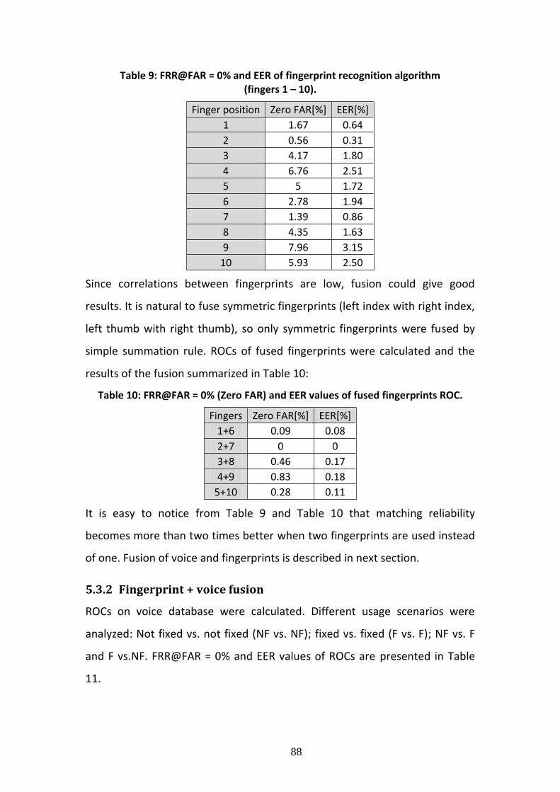
88

Table 9: FRR@FAR = 0% and EER of fingerprint recognition algorithm (fingers 1 – 10).

Finger position Zero FAR[%] EER[%]

1 1.67 0.64

2 0.56 0.31

3 4.17 1.80

4 6.76 2.51

5 5 1.72

6 2.78 1.94

7 1.39 0.86

8 4.35 1.63

9 7.96 3.15

10 5.93 2.50

Since correlations between fingerprints are low, fusion could give good

results. It is natural to fuse symmetric fingerprints (left index with right index,

left thumb with right thumb), so only symmetric fingerprints were fused by

simple summation rule. ROCs of fused fingerprints were calculated and the

results of the fusion summarized in Table 10:

Table 10: FRR@FAR = 0% (Zero FAR) and EER values of fused fingerprints ROC.

Fingers Zero FAR[%] EER[%]

1+6 0.09 0.08

2+7 0 0

3+8 0.46 0.17

4+9 0.83 0.18

5+10 0.28 0.11

It is easy to notice from Table 9 and Table 10 that matching reliability

becomes more than two times better when two fingerprints are used instead

of one. Fusion of voice and fingerprints is described in next section.

5.3.2 Fingerprint + voice fusion

ROCs on voice database were calculated. Different usage scenarios were

analyzed: Not fixed vs. not fixed (NF vs. NF); fixed vs. fixed (F vs. F); NF vs. F

and F vs.NF. FRR@FAR = 0% and EER values of ROCs are presented in Table

11.

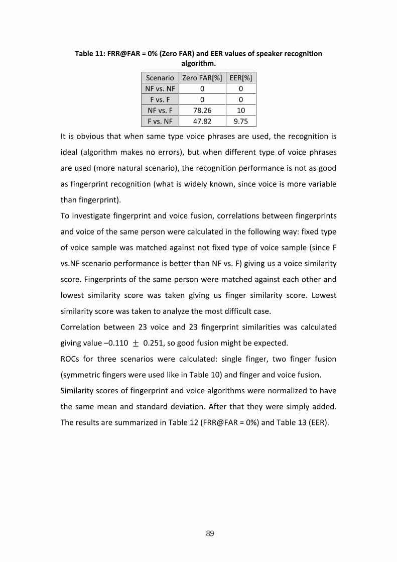
89

Table 11: FRR@FAR = 0% (Zero FAR) and EER values of speaker recognition algorithm.

Scenario Zero FAR[%] EER[%]

NF vs. NF 0 0

F vs. F 0 0

NF vs. F 78.26 10

F vs. NF 47.82 9.75

It is obvious that when same type voice phrases are used, the recognition is

ideal (algorithm makes no errors), but when different type of voice phrases

are used (more natural scenario), the recognition performance is not as good

as fingerprint recognition (what is widely known, since voice is more variable

than fingerprint).

To investigate fingerprint and voice fusion, correlations between fingerprints

and voice of the same person were calculated in the following way: fixed type

of voice sample was matched against not fixed type of voice sample (since F

vs.NF scenario performance is better than NF vs. F) giving us a voice similarity

score. Fingerprints of the same person were matched against each other and

lowest similarity score was taken giving us finger similarity score. Lowest

similarity score was taken to analyze the most difficult case.

Correlation between 23 voice and 23 fingerprint similarities was calculated

giving value –0.110 0.251, so good fusion might be expected.

ROCs for three scenarios were calculated: single finger, two finger fusion

(symmetric fingers were used like in Table 10) and finger and voice fusion.

Similarity scores of fingerprint and voice algorithms were normalized to have

the same mean and standard deviation. After that they were simply added.

The results are summarized in Table 12 (FRR@FAR = 0%) and Table 13 (EER).

90

Table 12: Comparison of three scenarios FRR @ FAR = 0% [%].

Single Finger Two

Fingers Finger and

Voice

1 1.67 1+6 0.09 1 0%

2 0.56 2+7 0 2 0%

3 4.17 3+8 0.46 3 0.22%

4 6.76 4+9 0.83 4 1.89%

5 5 5+10 0.28 5 0.67%

6 2.78 6+1 0.09 6 1.11%

7 1.39 7+2 0 7 0%

8 4.35 8+3 0.46 8 0.56%

9 7.96 9+4 0.83 9 1%

10 5.93 10+5 0.28 10 0.33%

Table 13: Comparison of three scenarios EER [%].

Single Finger Two

Fingers Finger and

Voice

1 0.64 1+6 0.08 1 0%

2 0.31 2+7 0 2 0%

3 1.80 3+8 0.17 3 0.11%

4 2.51 4+9 0.18 4 0.43%

5 1.72 5+10 0.11 5 0.25%

6 1.94 6+1 0.08 6 0.45%

7 0.86 7+2 0 7 0%

8 1.63 8+3 0.17 8 0.23%

9 3.15 9+4 0.18 9 0.22%

10 2.50 10+5 0.11 10 0.21%

It can be seen from Table 12 and Table 13 that in all cases finger and voice

fusion performers better than single fingerprint no matter what characteristic

(Zero FAR or EER) is considered.

In cases where correlation between two fingers is high, voice and fingerprint

fusion performs even better than two fingerprints fusion (see Table 12 row 1

(single fingerprint – 0.64%, two fingerprints – 0.09%, voice and fingerprint –

0%), row 3(single fingerprint – 4.17%, two fingerprints – 0.46%, voice and

fingerprint – 0.22%), and Table 13 rows 1 and 3).

91

5.4 Summary and Conclusions of the Chapter

Multibiometrics using fingerprints and voice was presented in this chapter.

Experiments show major increase in identification performance.

Multibiometric systems have many advantages over systems limited to only

one modality. They are more flexible and secure.

6 Conclusions

Fingerprint image synthesis method and two biometric algorithms (person

identification by fingerprints and speaker identification by voice) were

described in detail.

The speed of an earlier known synthesis algorithm has increased more than

three times. A new practical application of synthetic fingerprints to estimate

the quality of a fingerprint image by comparing it to an ideal noise free

synthetic fingerprint was found.

Problems in fingerprint matching are analyzed, and necessity of registration

(evaluation of rotation and translation) is discussed.

New Fingerprint matching algorithm is designed to match deformed

fingerprints. It consists of simple and intuitive steps. The proposed

implementation of the steps is straightforward and flexible, does not use

registration, and therefore is capable of matching deformed fingerprints. The

advantage of proposed fingerprint matching algorithm is validated on a set of

popular publically available fingerprint databases. One-tailed t-test showed

improvement in comparing with NIST matcher with p < 0.0005.

Speaker recognition algorithm uses phase of transfer function defined by

linear prediction model for derivation of features of utterances. The features

represent extremes of the group delay of the LP model. Similarity measure

between two speech utterances was defined as a mutual information of the

two group delay feature distributions.

92

The proposed voice recognition algorithm showed up to ten times better

performance in comparison with commonly accepted on Gaussian Mixture

Model based voice recognition algorithm.

Multibiometrics using fingerprints and voice was also presented. Experiments

showed significant decrease in EER and FRR@FAR = 0% when two fingerprints

or fingerprint and voice are used.

Voice and fingerprint fusion performs almost as well as two fingerprints

fusion.

This study is the first to demonstrate that similarities between voice samples

and similarities between fingerprints do not have any correlation what makes

them ideal for multibiometric.

6.1 Future Directions

Fingerprint synthesis method (chapter 2) can be used to create a fingerprint

with pre-defined properties and features. It would be interesting to

investigate the possibilities of synthesis to reconstruct low quality fingerprints

with scars, dirt and other imperfections.

During developing and testing of the fingerprint matching algorithm

(chapter3), minutiae features were limited to position and direction

information. Addition of other features (minutiae type, quality, texture

information) could further improve matcher performance.

It was shown that fingerprint fusion and voice fusion performs better than

fingerprints alone (chapter 5), and in some cases fingerprint and voice fusion

performs even better than fingerprint fusion. Such cases occur when

correlation between fingerprints is high. It would be useful to investigate such

occurrences and introduce additional normalization in fusion rule to account

fingerprint correlation.

93

Bibliography

[1] S. Pankanti and A. K. Jain.: Beyond Fingerprinting, Scientific American, 2008.

[2] A. K. Jain and J. Feng: Latent Palmprint Matching, IEEE Trans. on PAMI 2009.

[3] Anil K. Jain and Meltem Demirkus: On Latent Palmprint Matching, MSU Technical Report, 2008.

[4] L. D. Alsteris, K. K. Paliwal: Short-time phase spectrum in speech processing: A review and some experimental results. Digital Signal Processing 2007.

[5] A. M. Bazen, S. H. Gerez: Thin-plate spline modelling of elastic deformations in fingerprints. Proc. 3rd IEEE Benelux Signal Processing Symposium, 2002.

[6] A. Bastys, A. Kisel, A. Šalna: The use of group delay features of linear prediction model for speaker recognition. Informatica, 2010.

[7] R. Cappelli, D. Maio, D. Maltoni: Modelling plastic distortion in fingerprint images. Proceedings of the 2nd International Conference on Advances in Pattern Recognition, 2001.

[8] ELRA-S0050 Available at: http://www.linguistlist.org/issues/9/9-891.html, ELRA-S0050 Russian speech database (STC), 1998.

[9] T. Gambier-Langeveld: speaker recognition fake case evaluation. 8th Meeting of ENFSI Expert Working Group for Forensic Speech and Audio Analysis, Netherlands Forensic Institute, 2005.

[10] F. Itakura, S. Saito: Analysis synthesis telephony based upon the maximum likelihoood method. Reports on 6th Int. Conf. Acoust., 1968.

[11] Cai Jinhai, Jian Gangji, Zhang Lihe: New method for extracting speech formants using LPC phase spectrum. Electronic letters, 1993

[12] J. Kamarauskas: Speaker Recognition using Aussian Mizture Model, Electronics and Electrical Engineering, 5(85), January, 2008, 29-32.

[13] A. Kisel, A. Kochetkov, J. Kranauskas: Fingerprint Minutiae Matching without Global Alignment Using Local Structures. Informatica, 19(1), 2008, 31-44.

[14] D. Lee, K. Choi, J. Kim: A robust fingerprint matching algorithm using local alignment. In Proc. of 16th ICPR, 2002.

94

[15] A. Lipeika and J. Lipeikienė: Speaker identification using vector quantization. Informatica, 1995.

[16] A. Lipeika, J. Lipeikienė: Speaker Recognition Based on the Use of Vocal Tract and Residue Signal LPC Parameters. Informatica, 1999.

[17] D. J. C. MackKay: Information Theory, Inference, and Learning Algorithms. Cambridge University Press, 2003.

[18] A. Malickas, R. Vitkus: Fingerprint registration using composite features consensus. Informatica, 1999.

[19] D. Maio, D. Maltoni, R. Cappelli, J. L. Wayman, A. K. Jain: FVC2002: second fingerprint verification competition. Proceedings 16th International Conference on Pattern Recognition (ICPR2002), 2002.

[20] D. Maltoni, D. Maio, A. K. Jain, S. Prabhakar: “Handbook of fingerprint recognition. Springer”, 2003.

[21] D. Maltoni, D. Maio, A. K. Jain, and S. Prabhakar: "Handbook of Fingerprint Recognition", Second Edition, Springer, 2009.

[22] H. A. Murthy and B. Yeganarayana: Speech processing using group delay functions. Signal Processing, 1991.

[23] Neurotechnology MegaMatcher SDK Available at: http://www.neurotechnology.com/mm_sdk.html.

[24] N. K. Ratha, R. M. Bolle, V. D. Pandit, V. Vaish: Robust fingerprint authentication using local structural similarity. Fifth IEEE Workshop on. Applications of Computer Vision, 2000.

[25] D. A. Reynold, R. C. Rose: Robust Text-Independent Speaker Identification Using Gaussiam Mixture Speakers Models, IEEE transactions on speech and audio processing, 1995.

[26] S. Ribaric, I. Fratric, K. Kis: A Novel Biometric Personal Verification System Based on the Combination of Palmprints and Faces. Informatica, 2008.

[27] B. Šalna, J. Kamarauskas: Voice biometrics – evaluation of effectiveness of different methods in speaker recognition. In proc. of IEEE workshop on bio-inspired signal and image processing, 2008.

[28] A. Senior, R. Bolle: Improved fingerprint matching by distortion removal. IEICE Trans. Information and Systems, 2001.

[29] H. W. Strube: Linear prediction on a warped frequency scale, JASA, 1980.

[30] V. Struc, N. Pavesic: Gabor-Based Kernel Partial-Least-Squares Discrimination Features for Face Recognition. Informatica, 2009.

95

[31] T. Bourlai, A. Ross, and A. K. Jain: On Matching Digital Face Images Against Scanned Passport Photos, Proc. IEEE Int'l Conf. on Biometrics, Identity and Security (BIdS), 2009.

[32] T. Thiruvaran, E. Ambikairajah, J. Epps: Group Delay Features for Speaker Recognition. In Proc. Information, Communications & Signal Processing, 2007.

[33] C. I. Watson: NIST special database 29, plain and rolled images from paired fingerprint cards. U.S. National Institute of Standards and Technology (NIST), 2001.

[34] C. I. Watson, M. D. Garris, E. Tabassi, C. L. Wilson, R. M. McCabe, S. Janet: User's guide to NIST fingerprint image software 2 (NFIS2). National Institute of Standards and Technology (NIST), 2001.

[35] C. Watson, C. Wilson, K. Marshall, M. Indovina, R. Snelick: Studies of one-to-one fingerprint matching with vendor SDK matchers. National Institute of Standards and Technology (NIST), 2001.

[36] C. Wilson, R. A. Hicklin, H. Korves, B. Ulery, M. Zoepfl, M. Bones, P. Grother, R. Michaels, S. Otto, C. Watson:. Fingerprint vendor technology evaluation summary of results and analysis report. National Institute of Standards and Technology (NIST), 2004.

[37] A.-T. Yu and H.-Ch. Wang: Channel Effect Compensation in LSF Domain, EURASIP Journal on Applied Signal Processing, 2003.

[38] D. Maio, D. Maltoni, Cappelli, R., Wayman, J.L., A. K. Jain: FVC2000: Fingerprint Verification Competition, DEIS Technical Report, available online at: http://bias.csr.unibo.it/fvc. 2000.

[39] Jain, A.K., Prabhakar, S., Ross, A.: Fingerprint Matching: Data Acquisition and Performance Evaluation. MSU Technical Report, 1999.

[40] P. Jonathon Phillips, Martin Alvin, C. l. Wilson, Mark Przybocki: An Introduction to Evaluating Biometric Systems, Computer, February 2000.

[41] Biometrics Working Group: Best Practices in Testing and Reporting Performance of Biometric Devices, UK Government, (available online at: http://www.afb.org.uk/bwg/bestprac10.pdf.), 2000.

[42] C.L. Watson, C.L. Wilson: NIST Special Database 4, Fingerprint Database. NIST, 1992.

[43] C.L. Watson: NIST Special Database 14, Fingerprint Database. NIST, 1993.

96

[44] D. Maio, D. Maltoni: Direct Gray-Scale Minutiae Detection in Fingerprints, IEEE Transactions on Pattern Analysis and Machine Intelligence, 1997.

[45] F. Pernus, S. Kovacic, L. Gyergyek: Minutiae-Based Fingerprint Recognition, Proc. Fifth Int'l Conf. Pattern Recognition, 1980.

[46] X. Jiang et al.: Fingerprint Minutiae Matching Based on the Local And Global Structures. Proc. 15th Int'l Conf. Pattern Recognition, 2000.

[47] R. Cappelli, D. Maio, Maltoni, J.L. Wayman, Jain, A.K.: Performance evaluation of fingerprint verification systems. IEEE Transactions on Pattern Analysis and Machine Intelligence, 2006.

[48] D. Maio, D. Maltoni, R. Cappelli, J. L. Wayman, A. K. Jain: FVC2004: Third Fingerprint Verification Competition. Available online at: http://bias.csr.unibo.it/fvc2004/, 2004.

[49] P.J. Grother et al.: Minutiae Exchange Interoperability Test MINEX - Performance and Interoperability of the INCITES 378 Fingerprint Template. Technical Report NIST 7296, National Institute of Standards and Technology (NIST), available at: http://fingerprints.nist.gov/minex, 2006.

[50] R. Cappelli, D. Maio, D. Maltoni, A. Erol: Synthetic Fingerprint-Image Generation.

[51] C. J. Hill: Risk of Masquerade Arising from the Storage of Biometrics, B.S. Thesis, Australian National University (2001).

[52] J.L. Araque, M. Baena, B.E. Chalela, D. Navarro, P.R. Vizcaya: Synthesis of fingerprint images. Pattern Recognition, 2002.

[53] B.G. Sherlock, D.M. Monro: A model for interpreting fingerprint topology. Pattern Recognition, 1993.

[54] P.R. Vizcaya, L.A.Gerhardt: A nonlinear orientation model for global description of fingerprints. Pattern Recognition. 1999.

[55] J.K. Kamarainen: Feature extraction using Gabor filters. Ph.D. Dissertation, Lappeenranta University of Technology, 2003.

[56] John C. Russ: “Image Processing Handbook” 3rd ed. 1999.

[57] R. Cappelli, A. Lumini, D. Maio, and D. Maltoni: Fingerprint image reconstruction from standard templates, IEEE Trans. on Pattern Analysis and Machine Intelligence, 2007.

[58] C. I. Watson, C. L. Wilson: Effect of Image Size and. Compression on One-to-One. Fingerprint Matching. National Institute of Standards and Technology (NIST), 2005.

97

[59] H. W. Kuhn: The Hungarian method for the assignment problem. Naval Research Logistics Quarterly, 2(1-2):pp.83-97.

[60] Q. Li, B.-H. Juang, C.-H. Lee: Automatic verbal information verification for user authentication, IEEE Trans. on Speech and Audio Processing, 2000.

[61] G. M. White, R. Neely: Speech recognition experiments with linear prediction, bandpass filtering, and dynamic programming, IEEE Transactions on Acoustics, Speech and Signal Processing, 1976.

[62] R. L. Rabiner, A. E. Rosenberg, S. E. Levinson: Considerations in dynamic time warping algorithms for discrete word recognition, IEEE Transactions on Acoustics, 1978.

[63] D.A. Reynolds. Speaker identification and verification using Gaussian mixture speaker model. Speech Communication, 1995.

[64] T. Matsui and S. Furui: Comparison of text-independent speaker recognition methods using VQ-distortion and discrete/continuous HMMs, ICASSP, 1992.

[65] F. Bimbot and L. Mathan: Text-free speaker recognition using an arithmetic harmonic sphericity measure, Eurospeech, 1993.

[66] L. Rabiner, and B. H. Juang: An introduction to hidden Markov models, IEEE ASSP, 1986.

[67] F. Bimbot, at all: A tutorial on text-independent speaker verification. Journal on Applied Signal Processing, 2004.

[68] R. N. Bracewell: The Fourier Transform and Its Applications, 1999.

[69] A. V. Oppenheimand, R. W. Schafer: Discrete-Time Signal Processing, 1989.

[70] Fant Gunnar: Analysis and synthesis of speech processes. In Manual of phonetics, 1968.

[71] B. P. Bogert., M. J. R Healy., and J. W. Tukey: The frequency analysis of time series for echoes: cepstrum, pseudoautocovariance, cross-cepstrum and saphe cracking, in Proc. of the Symposium on Time Series Analysis, 1963.

[72] A. V. Oppenheim and R. W. Schafer: Homomorphic analysis of speech, IEEE Transactions on Audio and Electroacoustics, 1968.

[73] F. Itakura and S. Saito: Analysis synthesis telephony based upon the maximum likelihood method. Reports on 6th Int. Cong. Acoust., 1968.

[74] D. G. Childers, D. P. Skinner, and R. C. Kemerait: The Cepstrum. A Guide to Processing, Proceedings of the IEEE, 1977.

98

[75] S. Furui Comparison of speaker recognition methods using static features and dynamic features, IEEE Trans. Acoustics, Speech, and Signal Processing, 1981.

[76] R. Duda and P. Hart. “Pattern Classification and Scene Analysis”, 1973.

[77] F. K. Soong, A. E. Rosenberg, L. R. Rabiner, and B. H. Juang: A Vector Quantization Approach to Speaker Recognition. AT&T Technical Journal, pp. 14-26, 1987.

[78] A. Higgins, L. Bahler and J. Porter: Voice Identification Using Nearest Neighbor Distance Measure, In International Conference on Acoustics, Speech, and Signal Processing, 1993.

[79] B. H. Juang, L. R. Rabiner: Hidden Markov Models for Speech Recognition, Technometrics, 1991.

[80] D. A. Reynolds, and R. C. Rose: Robust Text-Independent Speaker Identification Using Gaussian Mixture Speaker Models, IEEE Transactions on Speech and Audio Processing, 1995.

[81] A. Lipeika, J. Lipeikienė: Speaker identification, 1993.

[82] A. Lipeika, J. Lipeikienė: Speaker identification using vector quantization. 1995.

[83] A. Lipeika, J. Lipeikiene: Speaker identification methods based on pseudo stationary segments of voiced sounds, 1996.

[84] R. M. Gray, A. Buzo, A. H. Gray, Y. Matsuyama: Distortion measures for speech processing, IEEE Trans. on Acoustic Speech and Signal Processing, 1980.

[85] A. Lipeika, J Lipeikienė: Speaker Recognition Based on the Use of Vocal Tract and Residue Signal LPC Parameters, 1999.

[86] A. Lipeika and J. Lipeikienė: Laiko skalės išlyginimas kalbos ir kalbančiojo atpažinime, Lietuvos matem. Rink. 2001.

[87] J. Kamarauskas: Speaker recognition using Gaussian Mixture Models, Electronics and Electrical Engineering, 2008.

[88] A. Rudžionis, V. Rudžionis: Consonant and speaker discrimination by consonant-vowel diphone components, Speaker Recognition in Telephony, 1996.

99

List of Tables

TABLE 1: DIFFERENCES BETWEEN MODIFIED SFINGE METHOD AND THE METHOD DESCRIED IN

[57]. ........................................................................................................... 47

TABLE 2: PROBABILITY OF SUCCESSFUL MATCHES [%]. ................................................. 48

TABLE 3: COMM+BOZORTH3 FRR @ FAR = 0.01% ON DIFFERENT PARTS OF SD29 ... 69

TABLE 4: COMM+ LSM FRR @ FAR = 0.01% ON DIFFERENT PARTS OF SD29. ............. 69

TABLE 5: FRR @ FAR = 0.01% ON TESTED DATABASES WITH COMMERCIAL MINUTIAE

EXTRACTOR ................................................................................................... 70

TABLE 6: RECOGNITION OF RUSBASE SPEAKER, CASE 1, VOICE MAN, USING DIFFERENT

METHODS AND FEATURES ................................................................................ 82

TABLE 7: SPEAKER RECOGNITION USING PHASE SPECTRUM FEATURES AND OF MUTUAL

INFORMATION TYPE SIMILARITY. RUSBASE DATA SET, CASE 1 – 5 ......................... 83

TABLE 8:. CORRELATIONS BETWEEN FINGERPRINTS WITH DIFFERENT POSITIONS. ............... 87

TABLE 9: FRR@FAR = 0% AND EER OF FINGERPRINT RECOGNITION ALGORITHM (FINGERS 1

– 10). ......................................................................................................... 88

TABLE 10: FRR@FAR = 0% (ZERO FAR) AND EER VALUES OF FUSED FINGERPRINTS ROC.

.................................................................................................................. 88

TABLE 11: FRR@FAR = 0% (ZERO FAR) AND EER VALUES OF SPEAKER RECOGNITION

ALGORITHM. ................................................................................................. 89

TABLE 12: COMPARISON OF THREE SCENARIOS FRR @ FAR = 0% [%]. ......................... 90

TABLE 13: COMPARISON OF THREE SCENARIOS EER [%]. ............................................. 90

100

Acronyms

AFIS Automatic Fingerprint Identification System

FVC Fingerprint Verification Competition

NIST National Institute of Standards and Technology

MINEX Minutiae Interoperability Exchange Test

ROC Receiver Operating Characteristic

DET Detection Error Tradeoff

SFINGE Synthetic Fingerprint Generation

EDM Euclidean Distance Map

WSQ Wavelet Scalar Quantization

DPI Dots per Inch

FRR False Rejection Rate

FAR False Acceptance Rate

EER Equal Error Rate

NFIS2 NIST Fingerprint Image Software Version 2

GMM Gaussian Mixture Model

LP Linear Prediction

LPC Linear Prediction Coefficient

NFISRE Netherlands Forensic Institute Speaker Recognition Evaluation

RUSBASE Russian Speech Data voice