JOURNAL OF ENVIRONMENTAL ECONOMICS AND MANAGEMENT 21, 127-139 (1991)

Permanent versus Interim Regulations: A Game-Theoretic Analysis’

ARUN S.MALIK

Economic Research Service, USDA, 1301 New York Avenue Northwest, Washington, D. C. 20005

Received August 16,1989; revised November 2 ,199O

When a regulator anticipates learning about the benefits or costs of regulations over time, quest ions can be raised about the appropriate regulatory policy. This paper compares permanent and interim regulations in a setting with initially uncertain pollution damages, a fixed capital input, and costly enforcement. The analysis shows that neither policy is first-best. Condit ions under which one policy dominates the other are identified with the help of a simulation. The results indicate that permanent regulations may be preferable to interim regulations even when there is substantial uncertainty about damages. o 1991 Academic PWS,

IllC.

INTRODUCTION

Government agencies are frequently forced to regulate firms despite consider- able uncertainty about the benefits and costs of doing SO.~ In many cases, this uncertainty diminishes over time as more is learned about the regulated activities and their consequences. In such cases, questions can be raised about the choice of regulatory policy. Should the agency issue interim regulations that can be revised in the future as more is learned about benefits and costs? Or should it issue “permanent” regulations that it commits to ma intaining well into the future?

When the inputs needed by firms to comply with the regulations are freely variable, it is clear that the agency should issue interim regulations that are continually revised as better information is obtained about benefits and costs. However, when one or more of the inputs is fixed (or costly to adjust), as is typically the case, it is unclear which policy is socially preferable. An interim regulations policy then gives firms an incentive to behave strategically when choosing their fixed compliance inputs. For example, in the context of pollution control, firms may be able to lim it the magn itude of future changes in em ission standards by adopting an inflexible, capital-intensive technology to comply with the current standard.

When we recognize that regulations are costly to enforce, the appropriate regulatory policy becomes even less apparent. Issuing regulations that are likely to be revised in the future creates uncertainty for firms, giving them an incentive to

‘I thank Gregory Amacher, A. Myrick Freeman, Robert Schwab, seminar participants at Resources for the Future, and the referees of this Journal for their helpful comments on earlier versions of this paper. The opinions expressed are my own and not necessari ly those of the U.S. Department of Agriculture.

‘This has been true for a variety of U.S. environmental regulations. A good example is the Water Pollution Control Act of 1972; see Freeman [51.

127 0095-0696/91 $3.00

Copyright 0 1991 by Academic Press, Inc. All rights of reproduction in any form reserved.

128 ARUN S. MALIK

delay compliance until a final set of regulations is issued. This wait-and-see behavior by firms is likely to make it more expensive to enforce interim regulations than permanent ones.3

In an attempt to formally compare the properties of alternative regulatory policies, I analyze a simple two-period model that captures both the fixity of compliance inputs and the costliness of enforcement. The regulatory policies are modeled as games between the regulator and the firm, with each policy defining a different game. The game corresponding to the permanent regulations policy is referred to as the precommitment game, and the one corresponding to the interim regulations policy as the discretionary game.

The games are described in terms of pollution control regulations. In each game, the regulator’s problem is to choose emissions standards given uncertainty about the damages from emissions. Fixity is incorporated in the model by specifying a capital input whose quantity cannot be varied once it is adjusted by the firm. The quantity of pollutant emitted by the firm depends on the stock of this fixed input.

In terms of the environmental literature, the paper is most closely related to Yao’s [16] work on strategic responses to automobile emissions regulations. Yao examines the dynamics of technology-forcing regulations given technological un- certainty and asymmetric information about innovation capabilities. In contrast, the focus here is on the effects of costly enforcement and damage uncertainty on the choice of regulatory policy when technology is certain and information is symmetric. The paper is also related to Viscusi’s [14, 151 work on environmental policy choice under uncertainty. However, issues of noncompliance and strategic behavior do not arise in his models.

Analytically, the paper shares much in common with the macroeconomic litera- ture on monetary policy games (e.g., Kydland and Prescott [8] and Canzoneri [4]). It also has elements in common with the literature on multiperiod principal-agent models (e.g., Baron and Besanko [l] and Laffont and Tirole [91X4 The model analyzed here differs from these principal-agent models in that I allow for costly enforcement and, like Yao, assume that the regulator is restricted to policies that are politically and administratively feasible. Thus, the regulator cannot employ complex payoff schedules or issue future standards contingent on the realization of uncertain parameters. As a result, the issues raised by this model and the optimal strategies for the regulator differ from those for the principal-agent models.

THE MODEL

Compliance Costs

The representative firm’s costs, excluding outlays on the fixed capital input, are summarized by a restricted cost function C(x, k). This function gives the reduction in profits from holding pollutant emissions and the fixed input constant at x and k, respectively. C(a) can be formally derived from the risk-neutral firm’s profit-

3The prevalence of this wait-and-see behavior contributed to the difficulty in enforcing environmen- tal regulations in the 1970s (e.g., see [lo]).

4For an excellent survey of this literature, see Caillaud et al. [3].

PERMANENT VS INTERIM REGULATIONS 129

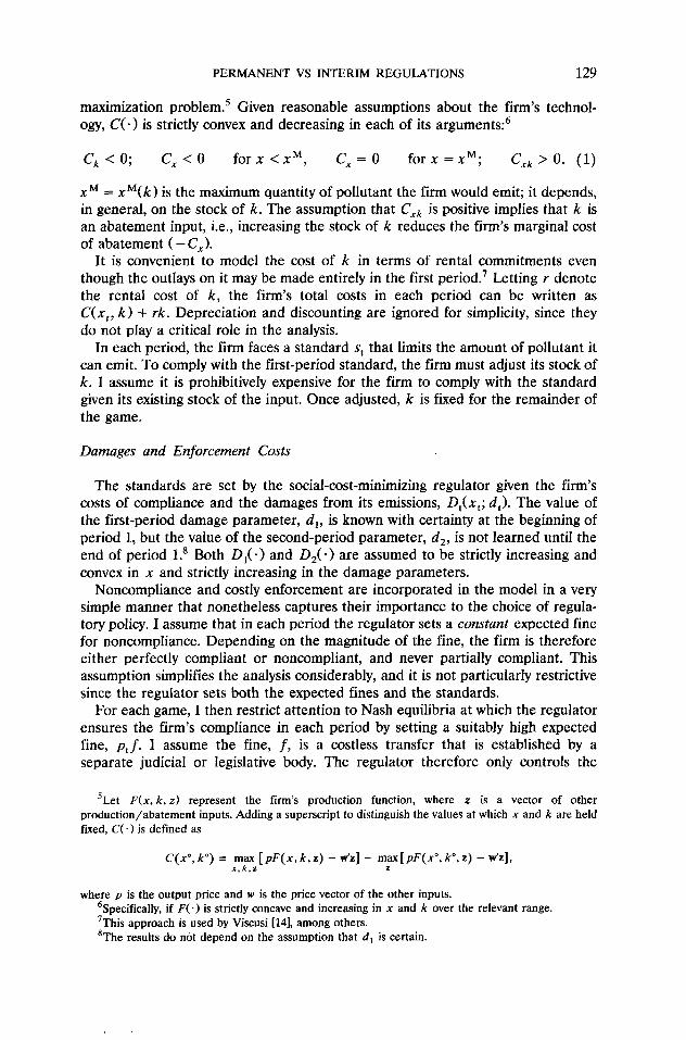
maximization problem.5 Given reasonable assumptions about the firm’s technol- ogy, C(* 1 is strictly convex and decreasing in each of its arguments?

c, < 0; c, < 0 for x <x”, c, = 0 for x =x~; Cxk ’ 0. (1)

xM = x”(k) is the maximum quantity of pollutant the firm would emit; it depends, in general, on the stock of k. The assumption that C,, is positive implies that k is an abatement input, i.e., increasing the stock of k reduces the firm’s marginal cost of abatement c-C,>.

It is convenient to model the cost of k in terms of rental commitments even though the outlays on it may be made entirely in the first period.’ Letting r denote the rental cost of k, the firm’s total costs in each period can be written as C(xI, k) + rk. Depreciation and discounting are ignored for simplicity, since they do not play a critical role in the analysis.

In each period, the firm faces a standard S, that lim its the amount of pollutant it can emit. To comply with the first-period standard, the firm must adjust its stock of k. I assume it is prohibitively expensive for the firm to comply with the standard given its existing stock of the input. Once adjusted, k is fixed for the remainder of the game.

Damages and Enforcement Costs

The standards are set by the social-cost-minimizing regulator given the firm’s costs of compliance and the damages from its emissions, D,(x,; d,). The value of the first-period damage parameter, d,, is known with certainty at the beginning of period 1, but the value of the second-period parameter, d,, is not learned until the end of period 1.8 Both D,(o) and D,(a) are assumed to be strictly increasing and convex in x and strictly increasing in the damage parameters.

Noncompliance and costly enforcement are incorporated in the model in a very simple manner that nonetheless captures their importance to the choice of regula- tory policy. I assume that in each period the regulator sets a constant expected fine for noncompliance. Depending on the magnitude of the fine, the firm is therefore either perfectly compliant or noncompliant, and never partially compliant. This assumption simplifies the analysis considerably, and it is not particularly restrictive since the regulator sets both the expected fines and the standards.

For each game, I then restrict attention to Nash equilibria at which the regulator ensures the firm’s compliance in each period by setting a suitably high expected fine, p,f. I assume the fine, f, is a costless transfer that is established by a separate judicial or legislative body. The regulator therefore only controls the

5Let F(x, k, z) represent the firm’s production function, where z is a vector of other production/abatement inputs. Adding a superscript to distinguish the values at which x and k are held fired, Cc.1 is defined as

c(p,k”) = xmkpxz[pF(x,k,z) - w’z] - max[M(n”,k”,z) - dzl, I 7 z

where p is the output price and w is the price vector of the other inputs. %pecifically, if F(.) is strictly concave and increasing in x and k over the relevant range. ‘This approach is used by Viscusi [14], among others. ‘The results do not depend on the assumption that d, is certain.

130 ARUN S. MALIK

probability of the fine, pt.9 The total costs of enforcement are given by &pt, where fit is the unit cost of raising the fine probability. Finally, I assume that all information is common knowledge and that the regulator can observe the firm’s choice of x and k.

COMMAND GAME

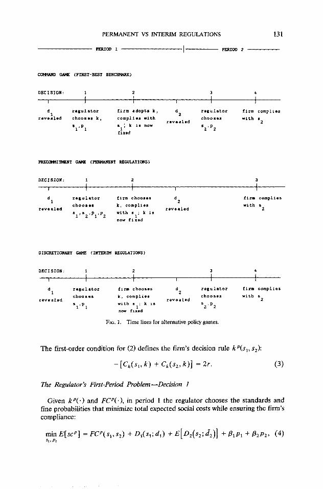
To begin, consider a benchmark game in which the regulator dictates both the pollutant standards and the firm’s stock of k, and sets the fine probabilities so that the firm is compliant. This command game corresponds, roughly, to a situation in which the regulator can specify the firm’s abatement technology, but the firm may delay adopting the technology and violate the standards if it does not face suitable penalties. The time line for the game is shown in Fig. 1.

The solution to this game, which I shall not characterize formally given space restrictions, is derived using a dynamic programming approach.” The solution is therefore time consistent; that is, there is no incentive for the regulator to change either the standards or the prescribed stock of k at any point during the game. Furthermore, since the regulator chooses k, the firm cannot engage in socially costly strategic behavior. As a result, the solution yields the first-best optimum given costly enforcement.

PRECOMMITMENT GAME

The regulator may be not be able to dictate the firm’s choice of k, however. In this case it could choose to play the precommitment game. In this game, the regulator issues both standards at the beginning of period 1 and makes a commit- ment not to modify them later on. The firm then sets its stock of k given these standards, The time line for the game is depicted in Fig. 1.

The Nash equilibrium for the game is characterized by the first-order conditions for the regulator’s and firm’s decision problems. The first-order conditions are derived sequentially, working backward from the last decision to the first.

The Firm’s Problem-Decisions 2 and 3

From Fig. 1, the firm’s decision to comply with s2 is the last one. The decision is a trivial one since the regulator ensures the firm’s compliance; thus, the firm simply sets its emissions x2 equal to s2.

In the next to last decision, the firm chooses the stock of k that minimizes its costs of complying with s1 and s2:

FCp(s,,s,) = mjn{C( sl, k) + C(s,, k) + 2rk). (2)

91 assume the regulator can commit to a fine probability that ensures the firm’s compliance. Although it is commonly assumed (implicitly) in the enforcement literature that the regulator can commit to punishment probabilities (e.g., see [7, ll]), it is not clear exactly how this is accomplished. As Guesnerie [6] points out, it could require some form of public lottery.

“The solution is conceptually similar to Yao’s [16] first-best benchmark.

PERMANENT VS INTERIM REGULATIONS 131

PERIOD 1 I P&RIOD 2

C- GAME (IXISI-BEST BENCIPIARK)

DECI SJON : 1 2 3 4 I I I I

I 1 I I

d d 1

r.gulator firm sdopts k, 2

regulator f irm complies tsvoslsd choosss k , complies with chooses

ravealsd with s

s .P ’ *l’

k is now 2 1 1 s2'p2

fixed

PRECC?WIIMENT GAME (PERMABENT REGULATIONS)

DECISION: 1 2 3

I I I I I

d regulator firm choosss d 1 2

firm complies choosss

r.vealed k, comp1i.s with s

revealed 2 sl’s2.Pl’P2 with I~; k is

now fixed

DISCRETIONARY GAME (INTERIM REGULATIONS 1

DECISION: 1 2 3 4 I I I I

I I

d 1

regulator firm chooses d 2

regulator firm compliss chooses k, complies chooses with L

revealed revealed 2 s1.p 1 with sl; Ir is s2. P 2

now fired

FIG. 1. Time lines for alternative policy games.

The first-order condition for (2) defines the firm’s decision rule k%,, sz):

-[C&1, k) + Ck(.Q, k)] = 2r. (3)

The Regulator’s First-Period Problem-Decision 1

Given kP( *) and FCP(.), in period 1 the regulator chooses the standards and fine probabilities that m inimize total expected social costs while ensuring the firm’s compliance:

n$y[scp] = FCp(s,,s,) +Dl(s,;d,) +E[D,(s,;&)] +&PI +@2P2, (4)

132 ARUN S. MALIK

s.t.

Plf 2 FCP(sl, %> - ([C(km X”( k,)) + rk,] + E[ Fc;(s;(d;))]), (5)

PJL [C(s,,kP) + rkp] - [C(X”(kP),kP) + rk”]. (6)

Constraint (6) ensures the firm’s compliance in period 2 by requiring the expected fine in this period to exceed the firm’s cost savings from noncompliance. The first term on the RHS gives the firm’s costs when it complies with s2 and the second term gives its costs when it does not. The second term can be explained as follows. Since I restrict attention to equilibria at which the firm is compliant, the firm would have been compliant in the first period and it would have anticipated being compliant in the second period. Therefore, it would have chosen its stock of k according to kp(+) in period 1. If, upon reaching period 2, the firm then decided to ignore the prevailing standard, it would choose the emission level that mini- mized its costs in this period. From (11, this emission level would be given by x”(kP). The firm’s second-period costs would therefore equal C(x”(kp), kP) + rkp.

Constraint (5) ensures the firm’s compliance in period 1. The RHS of the constraint gives the firm’s cost savings from noncompliance in this period. Once again, the firm would calculate these savings under the premise that it would become compliant in period 2. Thus, the expression in braces on the RHS of (5) gives the firms total costs if it delays compliance until period 2. The first term in braces can be explained as follows. Given the constant expected fine, the firm would not benefit from complying partially with si. Hence, the firm would not adjust its stock of k in period 1. It would simply choose the cost-minimizing emission level given its existing stock of k (if any), k,. From (11, this emission level would be x”(k,). The firm’s first-period costs would therefore equal C(x”(k,,>, k,) + rk,.

The firm’s second-period costs if it delays compliance are given by the second term in braces in (5). The derivation of this term is quite tedious and I have relegated it to the Appendix. Notice, however, that the term does not depend on the second-period standard announced at the beginning of the game, s2. This follows from the assumption that the regulator commits to s2 only if the firm is compliant in period 1. Otherwise, the regulator can revise s2 after d, is revealed. This seems more plausible than assuming that the regulator adheres to the preannounced standard even though the firm has not yet adjusted its stock of k.” (Note that the revised standard s;“(dJ is uncertain in period 1 since it depends on the value taken on by d2.)

Let wi and pZ be the Lagrange multipliers associated with constraints (5) and (6). The first-order conditions for pi and pZ imply that k1 = pi/f and pL2 = &/f.

“Although no formal proof is offered, not committing to the preannounced standard is likely to be the socially preferable alternative. Given the convexity of CT(.) in X, the attendant uncertainty about the second-period standard would lower the firm’s expected savings from noncompliance and thereby lower costs of enforcement.

PERMANENT VS INTERIM REGULATIONS 133

Using these equalities, the conditions for si and s2 can be written as

- (1 + Pl/f)C&,Y kP)

=-&(s,;d;)] + (P2/f)[W2,kP) - C,(x”(kp),kp)]g. (8) 2

These conditions together with (3) define the precommitment solution. Conditions (7) and (8) differ markedly from the simple rule that standards be set

to equate marginal abatement costs C-C,) and marginal damages. The extra terms here capture the effects of the standards on enforcement costs. Setting more lenient standards (i.e., increasing st) directly reduces enforcement costs in each period by lowering the costs of compliance. This effect is captured by the extra factor on the LHS of each condition. More lenient standards also induce the firm to choose a lower stock of k (dkP/&, < 0 given (3)). This indirectly raises enforcement costs in the second period by increasing the cost-savings from non- compliance in that period. This effect is captured by the extra term on the RHS of each condition. (The terms are positive since the bracketed expressions are negative given C,, > 0 and, presumably, s2 < x”.>

Properties of the Precommitment Solution

If damages were certain and enforcement were costless, the precommitment solution would clearly yield the first-best optimum. Conditions (7) and (8) would reduce to the usual requirement that marginal abatement costs and marginal damages be equated in each period. Moreover, the precommitment solution would be time consistent. Neither of these properties holds when costly enforcement or uncertain damages are incorporated.

Consider the effect of costly enforcement alone. As the discussion above makes clear, the firm’s choice of k influences the costs of enforcement. The firm, however, ignores these costs when choosing k. The regulator attempts to compen- sate for this externality by manipulating the standards, but this is socially costly since it affects compliance costs and pollution damages. As a result, the precom- mitment solution is not first-best.

It is also not time consistent. Once the firm has chosen k, there is an incentive for the regulator to cheat and change the previously announced second-period standard: the condition for the optimal standard at this point is given by (8) but without the last term.

The incentive to cheat is increased when uncertainty about damages is intro- duced. Upon learning the value of d, at the end of period 1, the regulator would almost surely want to change the second-period standard.

DISCRETIONARY GAME

Given the regulator’s incentive to cheat in the precommitment game, an alterna- tive game to consider is one in which the regulator only commits to the first-period

134 ARUN S. MALIK

standard at the beginning of the game. It does not issue the second-period standard until after the value of d, is learned. The firm must therefore choose k before the second-period standard is known. The time line for this discretionary game is shown in Fig. 1.

Once again, the first-order conditions characterizing the game’s Nash equilib- rium are derived sequentially, working backward from the last decision to the first. As in the precommitment game, the last decision (the fourth) is a trivial one where the firm sets its emissions equal to s2.

The Regulator’s Second-Period Problem-Decision 3

In the next to last decision, the regulator, having observed d,, minimizes second-period social costs while ensuring that the firm is compliant:

min sci = C( s2, k) + rk + D2( s2; d2) + &p2 %3P2

(9)

s.t. p2f a C(s,, k) - C(x”( k), k). (10)

Constraint (10) is virtually identical to (6) and can be explained similarly. Let A, be the Lagrange multiplier associated with (10). The first-order condition

for p2 implies that A, = &/f. Using this equality, the condition for s2 can be written as

-(l +P,/f)C,(s,,k) =Dds,;dd. (11) This condition is much simpler than the corresponding condition for the precom- mitment game, (8). Since sz is now issued after the firm chooses k, its stringency does not influence first-period enforcement costs and only influences second-period enforcement costs directly.

The Firm’s First-Period Problem-Decision 2

Let pi(k, d2) and s,d(k, d2) denote the decision rules defined by (10) and (11). Given s,“( .), in period 1 the firm will choose the stock of k that solves

EFCd(s,) = mp(E[C(sf(k,d;),k)] + C(s,,k) + 2rk>. (12)

The firm’s decision rule kd(s,) is defined by

-[C,(s,,k) +E[C,(s$(k,d;),k)]] = 2r+E Cx(~,d(ky&),k)f$ 1 . (13)

The primary difference between this condition and the corresponding condition for the precommitment solution (3) is the additional term on the RHS of (13). This term, which is positive, captures the firm’s strategic behavior: by choosing a small stock of k the firm can now induce the regulator to set a more lenient standard in period 2.12

“Differentiating (11) shows that as,d/ak < 0.

PERMANENT VS INTERIM REGULATIONS 135

The Regulator’s First-Period Problem-Decision 1

The regulator’s problem in period 1 is to m inimize total expected social costs while ensuring that the firm does not delay compliance:

m in E[ Scd] = EFCd( sl) + DI( s,; d,) + E[ D2( ii; d;)] S1r PI

+ PIP1 + PPq Isi] (14)

s.t. plf > EFCd(s,) - {[C(k,,, X”(k,)) + rk,,] + E[FC;(Q]}, (15)

where 5: = &kd, a,> and fig = p,d(kd, d;). The constraint (15) is identical to the one for the precommitment game, (5), except that the firm’s costs when compliant are now given by EFCd(s,); it can be justified similarly.‘3

Let A, denote the Lagrange multiplier associated with (15). The first-order condition for p1 implies that A, = /3,/f. The condition for s, can therefore be written as

II I $ 1

=D,,(s,;d,) + (P,/f)@&&kd) - C,(x”(kd),kd)]g. (16) 1

This condition together with (11) and (13) defines the dticretionary solution. The primary difference between (16) and the corresponding condition for the

precommitment solution (7) is the presence of the second term on the LHS of (16). This term, which has a positive sign, captures the regulator’s efforts to counter the firm’s strategic behavior. l4 It gives the expected second-period benefits of inducing the firm to choose a larger stock of k by making s1 more stringent (i.e., making s1 smaller).

Properties of the Discretionary Solution

Since the regulator sets s2 after the firm chooses k and after the uncertainty about damages is resolved, the discretionary solution is time consistent. It is not first best, however, given the firm’s socially costly strategic behavior when choosing k.15

WHICH GAME SHOULD THE REGULATOR PLAY?

The above results indicate that neither the precommitment solution nor the discretionary one is in general first best. The obvious question, then, is whether the

131n this discretionary game, the regulator always sets the second-period standard after d, is revealed and would take into account whether or not the firm had complied and adjusted its stock of k in the first period.

14Differentiating (13) shows that akd/as, < 0. 15A variant of the discretionary game would be one in which the regulator could control the firm’s

choice of k by punishing it for choosing the “wrong” k. This game would be very similar to the command game.

136 ARUN S. MALIK

regulator should play the precommitment game or the discretionary one. Unfortu- nately, drawing precise conclusions about the relative magnitude of expected social costs under the two games is difficult. However, a few observations can be made.

First, consider the simple case where damages are certain. It is not difficult to show that in this case the precommitment solution always yields lower expected social costs.16 (This is true with or without enforcement costs.) Putting off issuing the second-period standard does not yield any social benefits in this case. It simply gives the firm an opportunity to engage in strategic behavior, which is socially costly.

When uncertainty about damages is introduced, the relative magnitude of expected social costs at the two solutions becomes ambiguous. If we assume that enforcement is costless, then, as illustrated by an example in the next section, the relative magnitude of social costs depends on the degree of uncertainty about d,. If uncertainty is high, the discretionary solution yields lower expected social costs than the precommitment solution, while the opposite is true if uncertainty is low. In the latter case, the flexibility offered by the discretionary game is offset by the social costs associated with the firm’s strategic behavior.

The situation becomes more complicated when we add costly enforcement to the damage uncertainty. The relative magnitude of enforcement costs under the two games must now be determined. Although second-period enforcement costs are difficult to compare, one can argue that first-period enforcement costs are likely to be higher in the discretionary game because of the incentive it gives the firm to adopt a wait-and-see attitude and delay compliance.

It should be clear from the above discussion that the possible superiority of the discretionary solution is a function solely of the regulator’s ability to set the second-period standard after the uncertainty about damages is resolved.” If the standard had to be set before the uncertainty was resolved (but after the firm chose k), the discretionary solution would always be dominated by the precommit- ment one. This can be established using an argument similar to the one used earlier in the case of certain damages.

AN EXAMPLE

The above observations can be made more concrete by considering the following example. Let

C( x, k) = (1 - X)2/k0.5, Dl( x; d,) = dlx2, D2( x; d2) = d,x.

The results of a simulation based on these specifications are presented in Table I.

16The strategy of the proof is to specify a precommitment solution with the same standards as the discretionary one. Damages at this solution are the same as at the discretionary one but the firm’s costs are lower because it takes the standards as given when choosing the cost-minimizing stock of k. Enforcement costs are also lower because of the lower compliance costs.

t71f the regulator could commit to a schedule of second-period standards contingent on the value taken on by the damage parameter (a possibility I have ruled out because it is unlikely to be administratively feasible), the resulting precommitment solution would always dominate the discre- tionary one. However, the solution would not be first best given costly enforcement because the regulator would still not be able to costlessly control the firm’s choice of k. For an example of this approach in the context of monopoly regulation, see Baron and Myerson [2].

PERMANENT VS INTERIM REGULATIONS 137

TABLE I Differences in Expected Costs at the Precommitment and Discretionary Solutions (ESCP - ESCd)

P 0 1 2 3 9

0 - 0.080 - 0.034 0.010 0.054 0.297 1 - 0.048 -0.019 0.010 0.038 0.195 2 - 0.044 - 0.025 - 0.006 0.013 0.119 3 - 0.043 - 0.029 - 0.016 - 0.003 0.071 4 - 0.041 -0.031 - 0.022 - 0.013 0.041

The parameter values used in the simulation are d, = 10, & = 3, f = 4, k, = 0, and r = 10, along with the values specified in Table I.‘* Marginal enforcement costs for the two periods are equal (/3r = & = p>.

The entries in Table I give the differences in expected social costs at the precommitment and discretionary solutions. (The underlying expected social costs range from 6.247 to 9.441.) These cost differences are calculated for several values of the marginal cost of enforcement and of the variance of C$ (the relevant measure of uncertainty in this case).

Examining the first column, one can see that the precommitment solution consistently dominates the discretionary one when d, is certain, as argued above. The entries in the first row show that when enforcement is costless, the precom- m itment solution dominates the discretionary one when uncertainty about d, is low, but not when it is high.

Examining Table I as a whole, one can see that in the general case where damages are uncertain and enforcement is costly, the pattern of cost differences is quite complicated. The discretionary solution dominates the precommitment one when enforcement is not very costly and there is substantial uncertainty about damages. When enforcement is very costly (p 2 3), the discrefionary solution is dominant only if uncertainty about damages is very high WCd,) = 9); otherwise the precommitment solution is dominant.

Although they are not presented here, enforcement costs are consistently lower at the precommitment solution, in both periods. Expected firms costs are also lower at this solution, except when enforcement is costless and uncertainty about damages is low Md,) = 0,1X Expected damages are generally higher, with the same exceptions as those just noted. Thus, the benefits of playing the discretionary game are primarily in the form of reduced expected damages.

CONCLUDING OBSERVATIONS

The above results demonstrate that whether the regulator should play the discretionary game or the precommitment one depends, in a fairly complicated manner, on the uncertainty about damages and on the costs of enforcement. It is clear, however, that when enforcement is costly the precommitment game may be

“When x = 1 and k = 0, C(x, k) is set to equal to zero. For the parameter values chosen, it is always optimal for the regulator to restrict emissions in the first period, rather than to wait until the second period when the damage uncertainty is resolved.

138 ARUN S. MALIK

preferable to the discretionary one even if there is considerable uncertainty about damages.

A question I have thus far avoided is whether the precommitment solution is in fact feasible; that is, can the regulator credibly commit to the announced second- period standard given its ex post incentive to cheat? The nature of this commit- ment problem and possible solutions to it are similar to ones discussed in other contexts (e.g., see [4, 12, 161). Among the solutions that have been suggested is having the relevant legislative body tie the regulator’s hands by passing legislation specifying that standards cannot be modified over a suitable period of time. Another solution, which could be applied in a repeated game setting, is for the regulator to build a reputation for adhering to its preannounced standards.

Even if the precommitment solution is feasible, the analysis demonstrates that neither it nor the discretionary one yields the first-best optimum. In general, this is attained only when the regulator can specify the firm’s stock of k. An interesting implication of this result is that in an uncertain world with costly enforcement, an argument can be made for having the regulator prescribe the abatement technol- ogy the firm should employ. This is not true in the static, costless enforcement settings in which pollution control policies have typically been examined. In the arguably more realistic setting considered here, there are clear social benefits to having the regulator specify abatement technologies, provided, of course, that the underlying assumption of symmetric information about compliance costs is met. In practice, fairly accurate information about these costs is frequently available to the regulator. Moreover, it is not uncommon for existing regulatory policies to either recommend or specify abatement technologies. It may therefore be feasible in some cases to implement policies that yield the first-best optimum.

APPENDIX

The firm’s second-period costs if it delays compliance depend on: (i) the regulator’s ability to revise the second-period standard if the firm is noncompliant in period 1 and does not adjust its stock of k, and (ii) the regulator’s information about the firm’s first-period compliance status. As noted in the text, I assume that the regulator can revise the second-period standard if the firm is noncompliant in period 1. I also assume, for simplicity, that at the end of period 1 the regulator knows whether the firm has adjusted its stock of k.19 This implies that the regulator conducts a cursory inspection of the firm at least once while the first-period standard is in effect.20

“The analysis can be generalized to allow for the possibility that the regulator does not know the firm’s first-period compliance status. However, this complicates the analysis considerably without adding much insight.

“It does not imply that the first-period fine probability must equal one. In practice, there are numerous technical and legal hurdles that must be cleared before a fine can be imposed. The costs of conducting cursory audits that determine whether or not a firm has installed the necessary abatement equipment are much lower than the costs of taking the firm to court and ensuring that it is fined. As a result, many detected violations go unpunished. See Russell et al. 1131.

PERMANENT VS INTERIM REGULATIONS 139

Given these assumptions, in the second period, the noncompliant firm would choose the stock of k that solves

where ~2” is the revised second-period standard. Let kl(~z) denote the decision rule defined by this problem.

Given k,“(e), the regulator would choose the revised standard that m inimizes expected second-period social costs. 21 Let si(d2) denote the decision rule for the revised standard. Hence, from the perspective of the first period, when d, is uncertain, the firm’s expected second-period costs would be given by E[FC;(s2”(d2Nl.

REFERENCES

1. D. P. Baron and D. Besanko, Regulation and information in a continuing relationship, Inform. Econom. Policy 1,267-302 (1984).

2. D. P. Baron and R. Myerson, Regulating a monopolist with unknown costs, Econometrica 50, 911-930 (1982).

3. B. Caillaud, R. Guesnerie, P. Rey, and J. Tirole, Government intervention in production and incentives theory: A review of recent contributions, Rand J. Econom. 19, 1-26 (1988).

4. M. B. Canzoneri, Monetary policy games and the role of private information, Amer. Econom. Reu. 75, 1056-1070 (1985).

5. A. M. Freeman, Air and water pollution policy, in “Current Issues in U.S. Environmental Policy” (Paul R. Portney, Ed.), Johns Hopkins Univ. Press, Baltimore (1978).

6. R. Guesnerie, Hidden actions, moral hazard and contract theory, in “Allocation, Information, and Markets” (J. Eatwell et al., Eds.), Norton, New York (1989).

7. W. Harrington, Enforcement leverage when penalties are restricted, J. Public Econom. 37, 29-53 (1988).

8. F. Kydland and E. Prescott, Rules rather than discretion: The inconsistency of optimal plans, J. Polit. Econom. 85, 473-491 (1977).

9. J. J. Laffont and J. Tirole, The dynamics of incentive contracts, Econometrica 56, 1153-1175 (1988). 10. R. S. Melnick, “Regulation and the Courts: The case of the Clean Air Act,” Chaps. 2 and 7, The

Brookings Institution, Washington, DC (1983). 11. A. M. Polinsky and S. Shavell, The optimal tradeoff between the probability and magnitude of

fines, Amer. Econom. Rev. 69, 880-891 (1979). 12. J. F. Reinganum and N. L. Stokey, Oligopoly extraction of a common property natural resource:

The importance of the period of commitment in dynamic games, Internat. Econom. Rev. 26, 161-173 (1985).

13. C. S. Russell, W. Harrington, and W. J. Vaughan, “Enforcing Pollution Control Laws,” Chaps. 1 and 2, Resources for the Future, Washington, DC (1986).

14. W. K. Viscusi, Irreversible environmental investments with uncertain benefit levels, J. Environ. Econom. Management 15, 147-157 (1988).

15. W. K. Viscusi, Environmental policy choice with an uncertain chance of irreversibility, J. Enuiron. Econom. Management 12, 28-44 (1985).

16. D. A. Yao, Strategic responses to automobile emissions control: A game-theoretic analysis, J. Environ. Econom. Management 15,419-438 (1988).

*‘The regulator’s problem would be identical to (9)-(10) with s2 replaced by s;, k replaced by k,“(s,“), and x”(k) replaced by .x”(k,h