periodic little’s law - columbia.eduww2040/pll_030618_sub.pdfcompanion we provide evidence in...

Submitted to Operations Researchmanuscript (Please, provide the manuscript number!)

Authors are encouraged to submit new papers to INFORMS journals by means ofa style file template, which includes the journal title. However, use of a templatedoes not certify that the paper has been accepted for publication in the named jour-nal. INFORMS journal templates are for the exclusive purpose of submitting to anINFORMS journal and should not be used to distribute the papers in print or onlineor to submit the papers to another publication.

Periodic Little’s LawWard Whitt

Industrial Engineering and Operations Research, Columbia University, [email protected]

Xiaopei ZhangIndustrial Engineering and Operations Research, Columbia University, [email protected]

Motivated by our recent study of patient-flow data from an Israeli emergency department (ED), we establish

a sample-path periodic Little’s law (PLL), which extends the sample-path Little’s law (LL) of Stidham

(1974). The ED data analysis led us to propose a periodic stochastic process to represent the aggregate ED

occupancy level, with the length of a periodic cycle being one week. Because we conducted the ED data

analysis over successive hours, we construct our PLL in discrete time. The PLL helps explain the remarkable

similarities between the simulation estimates of the average hourly ED occupancy level over a week, using

our proposed stochastic model fit to the data, to direct estimates of the ED occupancy level from the data.

We also establish a steady-state stochastic PLL, similar to the time-varying LL of Bertsimas and Mourtzinou

(1997) and Fralix and Riano (2010).

Key words: Little’s law, L= λW , periodic queues, service systems, data analysis, emergency departments

History : submitted on April 29, 2017; revisions: October 31, 2017, March 6, 2018

1. Introduction

Many service systems with customer response times extending over hours or days can be modeled as

periodic queues with the length of a periodic cycle being one week. Examples are hospitals wards,

order-fulfillment systems and loan-processing systems. In this paper we establish a periodic version

of Little’s law, which can provide insight into the performance of these periodic systems.

We formulate our periodic Little’s law (PLL) in discrete time, assuming that there are d discrete

time points within each periodic cycle. In discrete time, the PLL states that, under appropriate

1

Whitt and Zhang: Periodic Little’s Law2 Article submitted to Operations Research; manuscript no. (Please, provide the manuscript number!)

conditions,

Lk =∞∑j=0

λk−jFck−j,j, k= 0,1, . . . , d− 1, (1)

where d is the number of time points within each periodic cycle, Lk is the long-run average number

in system at time k, λk is the long-run average number of arrivals at time k, and F ck,j , j ≥ 0, is the

long-run proportion of arrivals at time k that remain in the system for at least j time points, which

can be viewed as the complementary cumulative distribution function (ccdf) of the length of stay

of an arbitrary arrival. The long-run averages are over all indices of the form k+md, m≥ 0. These

quantities λk, F ck,· and Lk are periodic functions of the time index k, exploiting the extension of these

periodic functions to all integers, negative as well as positive.

In many applications, time is naturally continuous, in which case the analog of (1) is

L(t) =

∫ c

0

λ(t)F c(t− s, s)ds, 0≤ t < c, (2)

where c is the length of each periodic cycle. When time is continuous, we can construct a discrete-

time version by letting there be d subintervals of equal length within each continuous-time periodic

cycle, which we can refer to as time periods. We then obtain discrete-time processes by appropriately

counting what happens in each time period. But neither equal-length time subintervals in continuous

time nor a continuous-time reference is needed to have a bonafide discrete-time system.

On the other hand, if time is actually continuous, then we can use the discrete-time sample-path

PLL to define what we mean by a corresponding continuous-time sample-path PLL: we say that a

continuous-time PLL holds with (2) if the discrete-time PLL holds for all sequences of versions with

d periods in each continuous-time cycle with d→∞ and there is sufficient regularity in the limit

functions so that the limits in (1) can serve successive Riemann sums converging to the integral (2);

see §2.7 for further discussion.

We were motivated to develop the PLL because of a remarkable similarity between two curves

we observed in our recent study of patient-flow data from an Israeli emergency department (ED)

in Whitt and Zhang (2017a). As part of that study, we developed an aggregate stochastic model of

Whitt and Zhang: Periodic Little’s LawArticle submitted to Operations Research; manuscript no. (Please, provide the manuscript number!) 3

an emergency department (ED) based on a statistical analysis of patient arrival and departure data

from the ED of an Israeli hospital, using 25 weeks of data from the data repository associated with

the study by Armony et al. (2015). In §6 of Whitt and Zhang (2017a), we conducted simulation

experiments to validate the aggregate model of ED patient flow. One of these comparisons compared

direct estimates of the average ED occupancy level from data to estimations from simulations of the

stochastic model, where the distributions of the daily number of arrivals, the arrival-rate function

and the LoS distribution are estimated from the data. Figure 1 below shows that the two curves are

barely distinguishable. The PLL provides an explanation.

010

20

30

40

50

60

time of a week

num

ber

of patients

Sun Mon Tue Wed Thu Fri Sat

Estimated mean from dataEstimated mean from simulation

Figure 1 A comparison of the estimated mean ED occupancy level from (i) simulations of multiple replications

of the model fit to the data to (ii) direct estimates from the data.

In Whitt and Zhang (2017a), we suggested that this remarkable fit could be explained, at least

in part, by the time-varying Little’s Law (time-varying LL) from Bertsimas and Mourtzinou (1997)

and Fralix and Riano (2010). In this paper we elaborate on that idea by providing the new sample-

path version of PLL, because we think it may be important for constructing data-generated models

of service systems more broadly. While our primary focus here is on the PLL, in §3.4 and the e-

companion we provide evidence in support of the model we proposed in Whitt and Zhang (2017a).

The main contribution of this paper is the sample-path PLL in discrete time, Theorem 1, extending

the sample-path Little’s law (LL, L = λW ) established by Stidham (1974); also see El-Taha and


Stidham (1999), Fiems and Bruneel (2002), Little (1961, 2011), Whitt (1991, 1992) and Wolfe and

Yao (2014). This sample-path PLL is different in detail from all previous sample-path LL results

(known to us). For example, in addition to the usual limits of averages of the arrival rates and LoS

(waiting times), we need to assume a limit for the entire LoS distribution. The necessity of this

condition is shown by Example 1 in §2.4.

We also establish steady-state stochastic versions of the PLL, which relate more directly to the

time-varying LL in Bertsimas and Mourtzinou (1997) and Fralix and Riano (2010). This involves the

usual two forms of stationarity associated with arrival times and arbitrary times, that emerges from

the Palm theory of stochastic point processes; e.g., see Baccelli and Bremaud (1994) and Sigman

(1995), but now both are in discrete time, as in Section 1.7.4 of Baccelli and Bremaud (1994) and

Miyazawa and Takahashi (1992). Our steady-state stochastic versions of the PLL extend (and are

consistent with) an early PLL for the Mt/GI/1 queue in Proposition 2 of Rolski (1989).

The rest of the paper is organized as follows: In §2 we state and discuss the sample-path PLL.

In §3, we establish the steady-state stochastic versions of the PLL. In §3.4 and the e-companion

we elaborate on the ED application, reviewing the model we built in Whitt and Zhang (2017a),

illustrating how it relates to the PLL and providing evidence that the conditions in the theorems

are satisfied in our application. In §4 we provide the proofs of theorems in §2. Finally in §5 we draw

conclusions.

2. Sample-Path Version of the Periodic Little’s Law

In this section we develop the sample-path PLL. This version is general in that (i) we do not directly

make any stochastic assumptions and (ii) we do not directly impose any periodic structure. Instead,

we assume that natural limits exist, which we take to be with probability 1 (w.p.1). It turns out that

the periodicity of the limit emerges automatically from the assumed existence of the limits.

This section is organized as follows: In §2.1 we introduce our notation and definitions. In §2.2 we

state our main limit theorem. In §2.3 we discuss our assumptions and give an example showing that

the extra condition beyond what is needed for the LL is necessary. In §2.4 we establish a second


limit theorem showing that the natural indirect estimator for the average queue length based on the

arrival rate and waiting time is consistent. In §2.5 we establish a limit for the departure process as a

corollary to the main theorem. Finally, we conclude with some additional discussion to add insight. In

§2.6 we discuss the connection between our averages and associated cumulative processes. In §2.7 we

discuss the different orderings of events at discrete time points and the relation between continuous

time and discrete time.

2.1. Notation and Definitions

We consider discrete time points indexed by integers i, i ≥ 0. Since multiple events can happen

at these times, we need to carefully specify the order of events, just as in the large literature on

discrete-time queues, e.g., Bruneel and Kim (1993). We assume that all arrivals at one time occur

before any departures. Moreover, we count the number of customers (patients in the ED in our

intended application) in the system after the arrivals but before the departures. Thus, each arrival

can spend time j in the system for any j ≥ 0. Our convention yields a conservative upper bound on

the occupancy. We discuss other possible orderings of events and the relation between continuous

time and discrete time in §2.7.

With these conventions, we focus on a single sequence, X ≡ {Xi,j : i≥ 0; j ≥ 0}, with Xi,j denoting

the number of arrivals at time i that have length of stay (LoS) j. We also could have customers

at the beginning, but without lost of generality, we can view them as a part of the arrivals at time

0. We define other quantities of interest in terms of X. In particular, with ≡ denoting equality by

definition, the key quantities are:

Yi,j ≡∑∞

s=j Xi,s: the number of arrivals at time i with LoS greater or equal to j, j ≥ 0,

Ai ≡ Yi,0 =∑∞

s=0Xi,s: the total number of total arrivals at time i,

Qi ≡∑i

j=0 Yi−j,j =∑i

j=0Ai−j

Yi−j,j

Ai−j

: the number in system at time i,

all for i≥ 0. In the last line, and throughout the paper, we understand 0/0≡ 0, so that we properly

treat times with 0 arrivals.


We do not directly make any periodic assumptions, but with the periodicity in mind, we consider

the following averages over n periods:

λk(n) ≡1

n

n∑m=1

Ak+(m−1)d,

Qk(n) ≡1

n

n∑m=1

Qk+(m−1)d =1

n

n∑m=1

(k+(m−1)d∑

j=0

Yk+(m−1)d−j,j

),

Yk,j(n) ≡1

n

n∑m=1

Yk+(m−1)d,j, j ≥ 0,

F ck,j(n) ≡

Yk,j(n)

λk(n)=

∑n

m=1 Yk+(m−1)d,j∑n

m=1Ak+(m−1)d

, j ≥ 0, and

Wk(n) ≡∞∑j=0

F ck,j(n), 0≤ k≤ d− 1, (3)

where d is a positive integer.

Clearly, λk(n) is the average number of arrivals at time k, 0≤ k ≤ d− 1, over the first n periods;

Similarly, Qk(n) is the average number of customers in the system at time k, while Yk,j(n) is the

average number of customers that arrive at time k that have a LoS greater or equal to j. Thus,

F ck,j(n) is the empirical ccdf, which is the natural estimator of the LoS ccdf of an arrival at time k.

Finally, Wk(n) is the average LoS of customers that arrive at time k. We will let n→∞.

2.2. The Limit Theorem

With the framework introduced above, we can state our main theorem, the sample-path version of

the PLL. We first introduce our assumptions, which are just as in the sample-path LL, with one

exception. In particular, we assume that

(A1) λk(n)→ λk, w.p.1 as n→∞, 0≤ k≤ d− 1,

(A2) F ck,j(n)→ F c

k,j, w.p.1 as n→∞, 0≤ k≤ d− 1, j ≥ 0, and

(A3) Wk(n)→Wk ≡∞∑j=0

F ck,j w.p.1 as n→∞, 0≤ k≤ d− 1, (4)

where the limits are deterministic and finite. For the sample-path LL, d = 1 and we do not need

(A2).


The assumptions above only assume the existence of limits within the first period, but the limits

immediately extend to all k ≥ 0, showing that the limit functions must be periodic functions. We

then extend these periodic functions to the entire real line, including the negative time indices. We

give a proof of the following in §4.1.

Lemma 1. (periodicity of the limits) If the three assumptions in (4) hold, then the limits hold for all

k≥ 0, with the limit functions being periodic with period d.

We are now ready to state our main theorem; we give the proof in §4.2.

Theorem 1. (sample-path PLL) If the three assumptions (A1), (A2) and (A3) in (4) hold, then

Qk(n) defined in (3) converges w.p.1 as n→∞ to a limit that we call Lk. Moreover,

Lk =∞∑j=0

λk−jFck−j,j <∞, 0≤ k≤ d− 1, (5)

where λk and F ck,j are the periodic limits in (A1) and (A2) extended to all integers, negative as well

as positive.

Remark 1. (the extension to negative indices) To have convenient notation, we have extended the

periodic limit functions to the negative indices, but we do not consider the averages and their limits

in Assumptions (A1), (A2) and (A3) for negative indices.

2.3. The Assumptions in Theorem 1

When d= 1, the PLL reduces to the non-time-varying ordinary LL. In that case, k= 0 represents all

time indices since it is non-time-varying. In Theorem 1, L0 ≡ limn→∞

Q0(n) is the limiting time-average

number of customers in the system while limn→∞

λ0(n) = λ0 is the limiting average number of arrivals

at each time and the right hand side of (5) becomes

∞∑j=0

λk−jFck−j,j = λ0

∞∑j=0

F c0,j = λ0W0. (6)

And Theorem 1 claims that

L0 = λ0W0,


which is exactly the ordinary LL. Of course, the ordinary LL can be applied to the time-varying case

as well, but then we will lose the time structure and get overall averages.

There is a difference between our assumptions in (4) and the assumptions in the LL. For the LL,

we let L be the limiting time-average number in the system, λ be the limiting average arrival rate of

customers and W be the limiting customer-average waiting time (time spent in the system or length

of stay). Then, if both λ and W exist and are finite, then L exists and is finite, and L= λW . Our

limit for λk(n) in (A1) is the natural extension; the only difference is that now we require that λk(n)

converges w.p.1 for each k, 0≤ k ≤ d− 1. The third limit for Wk(n) in (A3) parallels the limit for

the average waiting time, but again we require that Wk(n) converges w.p.1 for each k, 0≤ k≤ d−1.

However, these two limits alone are not sufficient to determine the number of customers for the

periodic case. Now we need to require that the LoS distribution converges for each k, 0≤ k≤ d− 1,

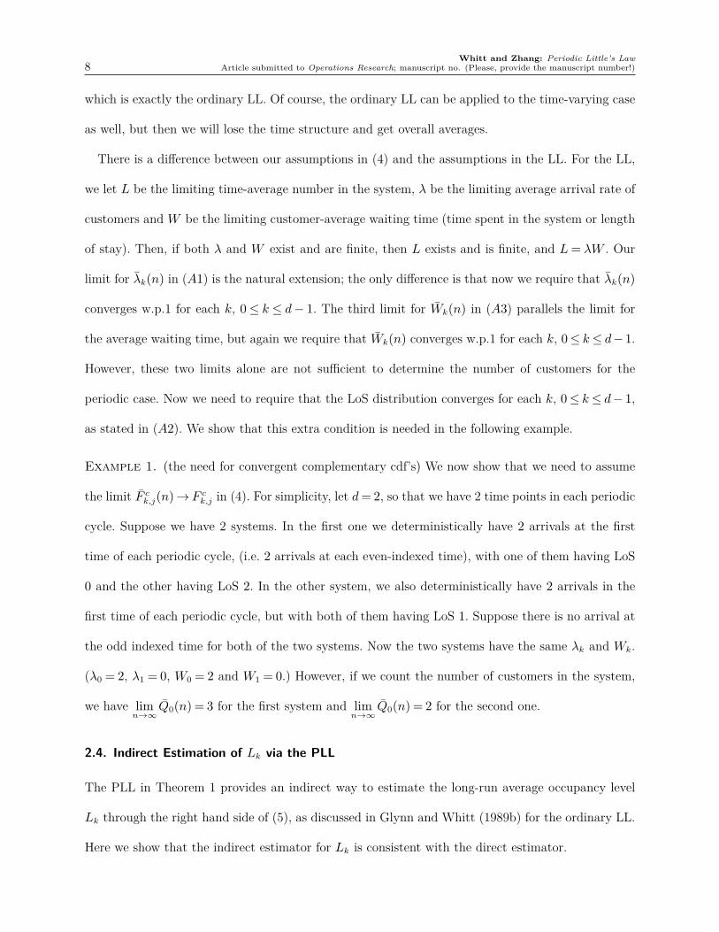
as stated in (A2). We show that this extra condition is needed in the following example.

Example 1. (the need for convergent complementary cdf’s) We now show that we need to assume

the limit F ck,j(n)→ F c

k,j in (4). For simplicity, let d= 2, so that we have 2 time points in each periodic

cycle. Suppose we have 2 systems. In the first one we deterministically have 2 arrivals at the first

time of each periodic cycle, (i.e. 2 arrivals at each even-indexed time), with one of them having LoS

0 and the other having LoS 2. In the other system, we also deterministically have 2 arrivals in the

first time of each periodic cycle, but with both of them having LoS 1. Suppose there is no arrival at

the odd indexed time for both of the two systems. Now the two systems have the same λk and Wk.

(λ0 = 2, λ1 = 0, W0 = 2 and W1 = 0.) However, if we count the number of customers in the system,

we have limn→∞

Q0(n) = 3 for the first system and limn→∞

Q0(n) = 2 for the second one.

2.4. Indirect Estimation of Lk via the PLL

The PLL in Theorem 1 provides an indirect way to estimate the long-run average occupancy level

Lk through the right hand side of (5), as discussed in Glynn and Whitt (1989b) for the ordinary LL.

Here we show that the indirect estimator for Lk is consistent with the direct estimator.


Since we only have data going forward in time from time 0, we start by rewriting (1) as

∞∑j=0

λk−jFck−j,j =

k∑i=0

λi

∞∑l=0

F ci,k−i+ld +

d−1∑i=k+1

λi

∞∑l=1

F ci,k−i+ld, 0≤ k≤ d− 1. (7)

Guided by (7), we let our indirect estimator for Lk be

Lk(n)≡k∑

i=0

λi(n)∞∑l=0

F ci,k−i+ld(n)+

d−1∑i=k+1

λi(n)∞∑l=1

F ci,k−i+ld(n), 0≤ k≤ d− 1, (8)

where λi(n) and F ci,j(n) are defined in (3). With data, it is likely that the infinite sums in (8)

would be truncated to finite sums, but at a level growing with n; we do not address that truncation

modification, which we regard as minor.

We now show that the estimator Lk(n) in (8) is asymptotically equivalent to the direct estimator

Qk(n) in (3); we will prove this result together with Theorem 1 in §4.2.

Theorem 2. (indirect estimation through the PLL) Under the conditions of Theorem 1,

limn→∞

Lk(n) =Lk w.p.1 for 0≤ k≤ d− 1, (9)

where Lk(n) is defined in (8) and Lk is as in Theorem 1.

In applications, the LoS often can be considered to be bounded, i.e., for some m> 1, Xi,j = 0 when

j ≥md. In that case, condition (A3) is directly implied by condition (A2) and it is possible to bound

the error between the direct and indirect estimators for Lk, defined as

Ek(n)≡ |Lk(n)− Qk(n)|, (10)

for Qk(n) in (3) and Lk(n) in (8), as we show now.

Corollary 1. (the bounded case) If, in addition to conditions (A1) and (A2) in Theorem 1, there

exists some mu > 0 such that Xi,j = 0 for i ≥ 0, j ≥ dmu, then assumption (A3) is necessarily

satisfied. If, in addition, there exists some λu > 0 such that Ai ≤ λu for i≥ 0, then

Rn ≡max0≤k≤d−1{Ek(n)} ≤λud(mu +2)2

2n, n≥mu, (11)

for Ek(n) in (10).


Proof: Here we show the proof of the first part of the corollary, i.e. if the LoS is bounded, then

assumption (A3) is implied from (A2), and we postpone the second half of proof until §4.3, since it

depends on part of the proof of Theorems 1 and 2.

If Xi,j = 0 for i≥ 0, j > dmu, then Fk,j(n) = 0 for 0≤ k≤ d− 1 and j ≥ dmu. So

Wk(n) =

dmu∑j=1

F ck,j(n), 0≤ k≤ d− 1,

is a finite summation and F ck,j = 0 for 0≤ k≤ d− 1 and j > dmu. Then

limn→∞

Wk(n) = limn→∞

dmu∑j=0

F ck,j(n) =

dmu∑j=0

limn→∞

F ck,j(n) =

dmu∑j=0

F ck,j =Wk,

which is assumption (A3).

Remark 2. (when (A2) implies (A3)) In addition to the boundedness condition presented in Corol-

lary 1, there are other mathematical conditions under which (A2) implies (A3), i.e., under which we

can interchange the order of the limits. Uniform integrability is a standard condition for this purpose;

see p. 185 of Billingsley (1995) and Section 2.6 of El-Taha and Stidham (1999). We prefer (A3) plus

(A2) because that makes our conditions easier to compare to the conditions in the ordinary LL.

2.5. Departure Processes

Besides relating the occupancy level with the arrival processes and the LoS as in the Little’s law, we

can also establish the relationship between the departure processes and the other quantities. This

will also be helpful to understand the error between different ways of counting what happens at each

time point, as we will explain in §2.7.

Let Di ≡∑i

j=0Xi−j,j , i≥ 0, be the number of departures at time i. Given the arrivals occur before

departures at each time, it is easy to see that

Di =Qi −Qi+1 +Ai+1, for i≥ 0. (12)

Paralleling (3), we look at the averages

δk(n)≡1

n

n∑m=1

Dk+(m−1)d, for 0≤ k≤ d− 1. (13)


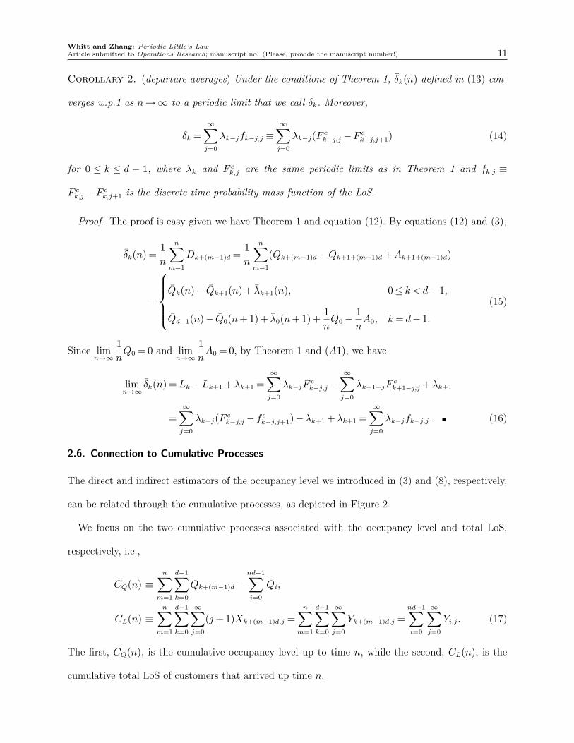
Corollary 2. (departure averages) Under the conditions of Theorem 1, δk(n) defined in (13) con-

verges w.p.1 as n→∞ to a periodic limit that we call δk. Moreover,

δk =∞∑j=0

λk−jfk−j,j ≡∞∑j=0

λk−j(Fck−j,j −F c

k−j,j+1) (14)

for 0 ≤ k ≤ d − 1, where λk and F ck,j are the same periodic limits as in Theorem 1 and fk,j ≡

F ck,j −F c

k,j+1 is the discrete time probability mass function of the LoS.

Proof. The proof is easy given we have Theorem 1 and equation (12). By equations (12) and (3),

δk(n) =1

n

n∑m=1

Dk+(m−1)d =1

n

n∑m=1

(Qk+(m−1)d −Qk+1+(m−1)d +Ak+1+(m−1)d)

=

Qk(n)− Qk+1(n)+ λk+1(n), 0≤ k < d− 1,

Qd−1(n)− Q0(n+1)+ λ0(n+1)+1

nQ0 −

1

nA0, k= d− 1.

(15)

Since limn→∞

1

nQ0 = 0 and lim

n→∞

1

nA0 = 0, by Theorem 1 and (A1), we have

limn→∞

δk(n) =Lk −Lk+1 +λk+1 =∞∑j=0

λk−jFck−j,j −

∞∑j=0

λk+1−jFck+1−j,j +λk+1

=∞∑j=0

λk−j(Fck−j,j − f c

k−j,j+1)−λk+1 +λk+1 =∞∑j=0

λk−jfk−j,j. (16)

2.6. Connection to Cumulative Processes

The direct and indirect estimators of the occupancy level we introduced in (3) and (8), respectively,

can be related through the cumulative processes, as depicted in Figure 2.

We focus on the two cumulative processes associated with the occupancy level and total LoS,

respectively, i.e.,

CQ(n) ≡n∑

m=1

d−1∑k=0

Qk+(m−1)d =nd−1∑i=0

Qi,

CL(n) ≡n∑

m=1

d−1∑k=0

∞∑j=0

(j+1)Xk+(m−1)d,j =n∑

m=1

d−1∑k=0

∞∑j=0

Yk+(m−1)d,j =nd−1∑i=0

∞∑j=0

Yi,j. (17)

The first, CQ(n), is the cumulative occupancy level up to time n, while the second, CL(n), is the

cumulative total LoS of customers that arrived up time n.


Figure 2 helps understand the two cumulative quantities. In the figure, we plot the time intervals

that each of the first 35 arrivals spends in the system as horizontal bars, each with height 1 placed

in order of the arrival times. The left end point is the arrival time, while the right end point is the

departure time, which need not be in order of arrival. We can see that CQ(n) and CL(n) correspond

to two areas respectively.

Figure 2 An example of a periodic queueing system with d = 5 and n = 4. The vertical line is placed at time

nd= 20. Area A corresponds to CQ(4) in (18) below, while Area A∪B corresponds to CL(4) in (18).

We can further relate the two cumulative processes to the averages in (3) and (8), as stated in the

following proposition.

Proposition 1. The cumulative processes and the averages are related by

Area(A) =CQ(n) = nd−1∑k=0

Qk(n),

Area(A∪B) =CL(n) = nd−1∑k=0

λk(n)Wk(n) = nd−1∑k=0

Lk(n). (18)


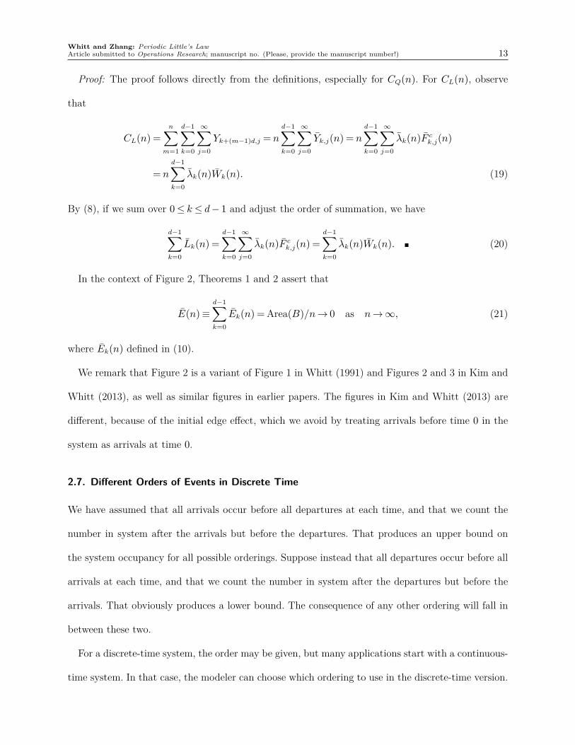
Proof: The proof follows directly from the definitions, especially for CQ(n). For CL(n), observe

that

CL(n) =n∑

m=1

d−1∑k=0

∞∑j=0

Yk+(m−1)d,j = nd−1∑k=0

∞∑j=0

Yk,j(n) = nd−1∑k=0

∞∑j=0

λk(n)Fck,j(n)

= nd−1∑k=0

λk(n)Wk(n). (19)

By (8), if we sum over 0≤ k≤ d− 1 and adjust the order of summation, we have

d−1∑k=0

Lk(n) =d−1∑k=0

∞∑j=0

λk(n)Fck,j(n) =

d−1∑k=0

λk(n)Wk(n). (20)

In the context of Figure 2, Theorems 1 and 2 assert that

E(n)≡d−1∑k=0

Ek(n) =Area(B)/n→ 0 as n→∞, (21)

where Ek(n) defined in (10).

We remark that Figure 2 is a variant of Figure 1 in Whitt (1991) and Figures 2 and 3 in Kim and

Whitt (2013), as well as similar figures in earlier papers. The figures in Kim and Whitt (2013) are

different, because of the initial edge effect, which we avoid by treating arrivals before time 0 in the

system as arrivals at time 0.

2.7. Different Orders of Events in Discrete Time

We have assumed that all arrivals occur before all departures at each time, and that we count the

number in system after the arrivals but before the departures. That produces an upper bound on

the system occupancy for all possible orderings. Suppose instead that all departures occur before all

arrivals at each time, and that we count the number in system after the departures but before the

arrivals. That obviously produces a lower bound. The consequence of any other ordering will fall in

between these two.

For a discrete-time system, the order may be given, but many applications start with a continuous-

time system. In that case, the modeler can choose which ordering to use in the discrete-time version.


We have chosen the conservative upper bound. In this section we derive an expression for the alter-

native lower bound and the difference between the upper bound and the lower bound. From that

difference, we can see that the difference between an initial continuous-time system and a discrete-

time “approximation” will become asymptotically negligible as we refine the discrete-time version by

increasing the number of discrete time points within a fixed continuous-time cycle.

For the alternative departure-first (lower-bound) ordering, let QLi be the number of customers in

the system at time i and let

QLk (n)≡

1

n

n∑m=1

QLk+(m−1)d. (22)

Assume that we keep the meaning of Xi,j and Yi,j .

Proposition 2. (the lower-bound occupancy) Under the conditions of Theorem 1, QLk (n) converges

w.p.1 as n→∞ to a limit that we call LLk , and we have

LLk =Lk − δk − 2λk +λkfk,0 ≤Lk for 0≤ k≤ d− 1, (23)

where Lk is in Theorem 1, λk is in (A1), δk and fk,0 are the same as in Corollary 2.

Proof. For the new departures-first ordering, the number of customers at time i is

QLi =

i∑j=1

Yi−j,j+1 −Yi,0 =i∑

j=1

Yi−j,j −i∑

j=1

Xi−j,j −Yi,0 =i∑

j=0

Yi−j,j −i∑

j=0

Xi−j,j − 2Ai +Xi,0

=Qi −Di − 2Ai +Xi,0, (24)

where we regard the summation as 0 if the lower bound is larger than the upper bound. By equation

(24) and (22), we have

QLk (n) =

1

n

n∑m=1

QLk+(m−1)d =

1

n

n∑m=1

(Qk+(m−1)d −Dk+(m−1)d − 2Ak+(m−1)d +Xk+(m−1)d,0)

= Qk(n)− δk(n)− 2λk(n)+ (Yk,0(n)− Yk,1(n)). (25)

Next observe that (A1) and (A2) imply that limn→∞

Yk,j(n) = λkFck,j , so that

limn→∞

QLk (n) =Lk − δk − 2λk +λk(F

ck,0 −F c

k,1) =Lk − δk − 2λk +λkfk,0. (26)


We can apply Proposition 2 to deduce that the error in an incorrect ordering of events is asymptot-

ically negligible if we start with a continuous-time system and choose sufficiently short time periods.

For the arrival process A(t), we assume that

t−1A(t)→Λ(t) as t→∞, (27)

where

Λ(t) =

∫ t

0

λ(u)du and 0<λU ≤ λ(u)≤ λU <∞, (28)

for all nonnegative u and t, with λ being a periodic function with period c. We make a similar

assumption for the departure process D(t) with the limiting rate being δ(t).

Corollary 3. (from continuous to discrete time) Suppose that we start with a continuous-time

periodic system with period c and construct a discrete-time system by considering d evenly spaced

time intervals within each periodic cycle. If the arrival and departure processes satisfy (27) and (28),

and if the conditions of Theorem 1 hold for each d, then the error in the discrete-time approximation

due to the order of events at each time point goes to 0 as d→∞.

Proof. From (23), we know that 0≤Lk −LLk = δk +2λk −λkfk,0. Hence, if we consider a sequence

of systems indexed by d, then the condition implies that λd,k → 0 and δd,k → 0 as d→∞.

We can use Corollary 3 to define what we mean by a continuous-time sample-path PLL. We also

exploit basic properties of Riemann integrals; see §6 of Rudin (1976).

Definition 1. (continuous-time sample-path PLL) Consider a continuous-time system with arrival

process having a periodic arrival rate and satisfying (27) and (28). A continuous-time sample-path

PLL holds, yielding relation (2), if

(i) the discrete-time PLL holds for each d when we form d time periods within each periodic cycle,

and

(ii) the sequence of discrete-time PLLs in (1) can be regarded as converging Riemann-sum approx-

imations for the continuous-time relation in (2).


3. Steady-State Stochastic Versions of the Periodic Little’s Law

We now discuss stochastic analogs of Theorem 1. In §3.1 we define a stationary framework in continu-

ous time. In §3.2 we derive a steady-state stochastic PLL by applying Theorem 1. In §3.3 we establish

a version of PLL for the Gt/GIt/∞ time-varying infinite-server model proposed in Whitt and Zhang

(2017a). In §3.4 we conduct additional analysis of the ED data to provide additional support for

the stochastic model proposed in Whitt and Zhang (2017a), despite the negligible support provided

by Figure 1. Finally, in §3.5 we establish a continuous-time stochastic PLL, which primarily follows

from Rolski (1989) and Fralix and Riano (2010).

For this initial version, we aim for simplicity. Thus, we assume that the basic stochastic process is

both stationary and ergodic, so that steady-state means coincide with long-run averages. The main

idea is that we now interpret the key quantities Lk and λk appearing in (1) as appropriate expected

values of random variables associated with the system in periodic steady state. As we see it, there

are two main issues:

1. What is meant by periodic steady state?

2. What is F ck,j or, equivalently, what is the probability distribution of the LoS of an arbitrary

arrival in period k?

3.1. Periodic Steady State

In order to construct periodic steady-state, we assume that the basic stochastic process {Yn : n∈Z}

with

Yn ≡ {Ynd+k,j : 0≤ k≤ d− 1; j ≥ 0} (29)

introduced in §2.1 is a stationary sequence of nonnegative random elements indexed by the integer

n. For each integer n, the random element Yn takes values in the space (Zd)∞ ≡Zd ×Zd × · · · . See

Chapter 6 of Breiman (1968) and Baccelli and Bremaud (1994), Sigman (1995) for background on

stationary processes and their application to queues. Just as for the time-varying LL, as discussed in

Fralix and Riano (2010), it is important to apply the Palm transformation, but we avoid that issue

by exploiting the established limits for the averages.


Without loss of generality, we now regard our stochastic processes as stationary processes on the

integers Z, negative as well as positive; see Proposition 6.5 of Breiman (1968). As usual, we mean

strictly stationary; i.e., the finite-dimensional distributions are independent of time shifts, which in

turn means that, for each k and each k-tuple (n1, . . . , nk) of integers in Z,

(Yn1, . . . ,Ynk

)d= (Yn1+m, . . . ,Ynk+m) for all m∈Z,

with d= denoting equality in distribution.

As a consequence of the stationarity assumed for {Yn : n ∈ Z}, we also have stationarity for the

associated stochastic process {(And+k,Qnd+k) : n∈Z}, where And+k is the number of arrivals at time

nd+k and Qnd+k is the number of customers in the system at time nd+k, both of which are defined

in §2.1, but now that we have stationarity on all integers, negative as well as positive. Thus, we have

And+k ≡ Ynd+k,0 and Qnd+k ≡∞∑j=0

Ynd+k−j,j.

Hence, with some abuse of notation, we let ({Yk,j : j ≥ 0},Ak,Qk) be a stationary random element.

In this stochastic setting, we have

λk ≡E[Ak] =E[Yk,0] and Lk ≡E[Qk] =∞∑j=0

E[Yk−j,j]. (30)

3.2. The Stochastic PLL

We now come to the second issue: In the stochastic setting it remains to define F ck,j ≡ P (Wk > j),

where Wk is the time in system for an arbitrary arrival in period k. It is natural to define F ck,j by

requiring that it agree with the limit of the averages F ck,j(n) in (3). That limit is well defined if we

assume that the basic sequence is ergodic as well as stationary, with 0<E[Yk,0]<∞ for all k.

With the stationary framework on all the integers, positive and negative, the stochastic PLL

becomes very elementary, because there are no edge effects.

Theorem 3. (stochastic PLL) Suppose that {Yn : n ∈ Z} in (29) is stationary and ergodic with

0<λk ≡E[Yk,0]<∞, 0≤ k≤ d− 1. Then, for each k, 0≤ k≤ d− 1, and j ≥ 0,

F ck,j(n)→ F c

k,j ≡E[Yk,j]

E[Yk,0]w.p.1 as n→∞ (31)


and

Lk ≡E[Qk] =∞∑j=0

λk−jFck−j,j. (32)

Proof. First, the stationary and ergodic condition with the specified moment assumptions implies

that

Yk,j(n)→E[Yk,j] = λkFck,j as n→∞ w.p.1

for all k and j in view of (3), (30) and the definition of F ck,j in (31). Then (31) follows immediately

by continuity under the division operation by a quantity with a strictly positive limit. If we multiply

and divide by λk within the representation for E[Qk] in (30), then we see that

E[Qk] =∞∑j=0

E[Yk−j,j] =∞∑j=0

λk

E[Yk−j,j]

λk

=∞∑j=0

λkFck−j,j.

In closing this section, we remark that the distribution Fk,j can be seen to be correspond to an

underlying Palm measure, but we do not develop that framework here; see Sigman and Whitt (2018).

3.3. The Discrete-Time Periodic Gt/GIt/∞ Model

The candidate model for the ED proposed in Whitt and Zhang (2017a) was a special case of the

periodic Gt/GIt/∞ infinite-server model, in which the LoS variables are mutually independent and

independent of the arrival process, with a ccdf F ck,j ≡ P (Wk ≥ j) for a steady-state LoS in time

period k that depends only on the time period k within the periodic cycle (a week). This strong local

condition provides a sufficient condition for the steady-state stochastic PLL. That can be seen from

the following proposition.

Proposition 3. (the Gt/GIt/∞ special case) For the stationary Gt/GIt/∞ infinite-server model

specified above, where Y≡ {Yn : n∈Z} in (29) is strictly stationary with finite mean values, then

E[Yk,j] = F ck,jE[Yk,0],

consistent with formula (31).


Proof. Let {Wk,i : i ≥ 1} be a sequence of i.i.d. LoS variables associated with arrivals in time

period k, which is also independent of the arrival process and the other LoS variables. Under those

conditions,

E[Yk,j] =∞∑

m=1

m∑i=1

P (Wk,i > j)P (Ak =m)

=∞∑

m=1

mF ck,jP (Ak =m) = F c

k,jE[Ak] = F ck,jE[Yk,0].

3.4. Further Statistical Tests of the Infinite-Server Model

We now report results directly testing the GIt assumption in the stochastic model proposed in Whitt

and Zhang (2017a). We briefly review the data analysis in the e-companion here.

Now we first test whether the LoS distribution in period k can be regarded as being independent

of the number of arrivals in period k. To be specific, let A(m)k be the number of arrivals in hour k

of week m, where in our ED case 1≤ k ≤ 7× 24 = 168 and m is from 1 to 25. And let W(i)k be the

average LoS of arrivals in hour k of week m. For each k, we compute the estimated (sample) Pearson

correlation coefficients of A(i)k and W

(m)k , using samples where A

(m)k > 0; See p.169 of Casella and

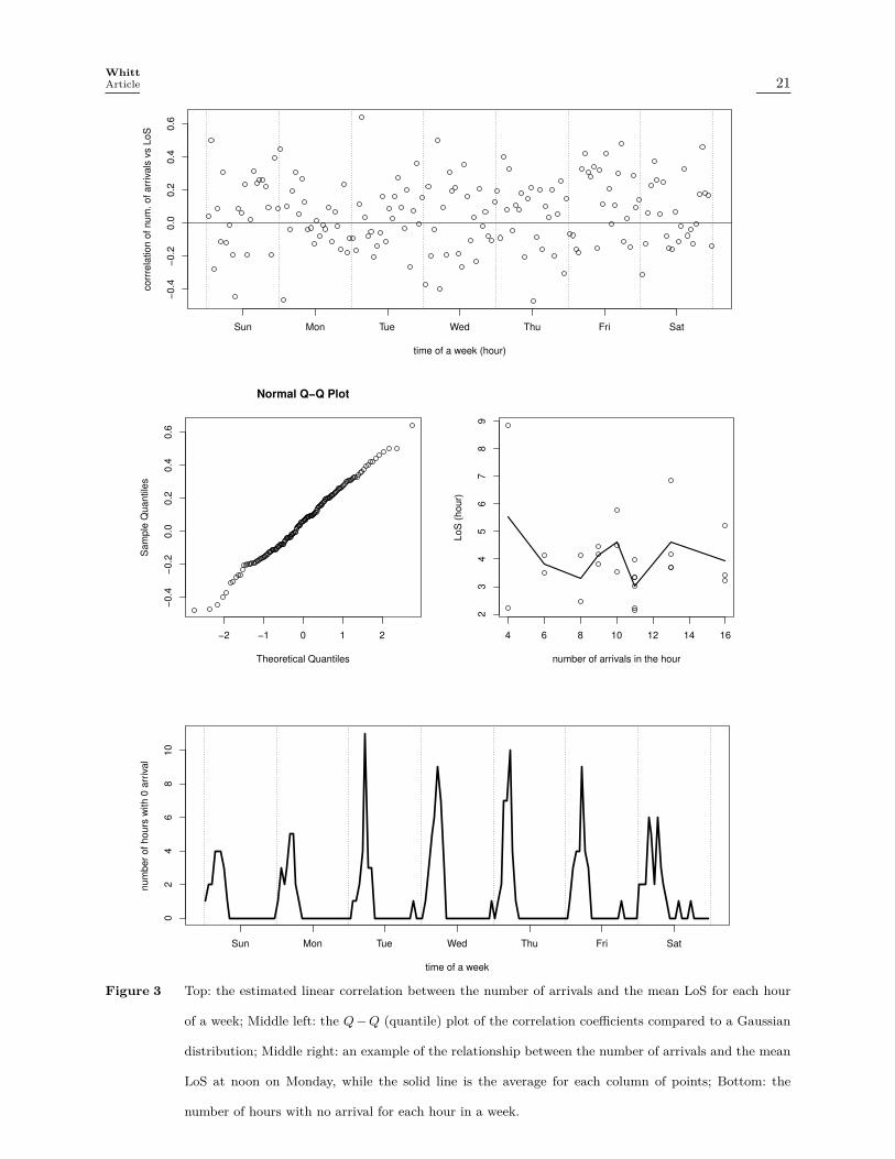
Berger (2002) for background. The plot in the top of Figure 3 shows the correlation coefficients (rk)

of all 168 hours in a week, where (if A(m)k > 0 for all m)

rk =

∑25

m=1(A(m)k − Ak)(W

(m)k − Wk)√∑25

m=1(A(m)k − Ak)2

√∑25

m=1(W(m)k − Wk)2

,

where Ak ≡ (1/25)∑25

i=1A(m)k and Wk ≡ (1/25)

∑25

i=1W(m)k . For any m such that A(m)

k = 0, we remove

those terms in the summation and the average correspondingly.

The middle left plot compares the quantile of the coefficients with the normal distribution, and

indicates that the distribution of the 168 correlation coefficients are approximately normal, with

sample mean 0.056 and sample standard error 0.21. It shows that there is no significant evidence

indicating that the LoS distribution is related to the number of arrivals within each hour. The middle

right plot is a scatter plot of (A(m)36 ,W

(m)36 ), i.e., at noon on Monday, excluding samples with no

arrivals, and the solid line is the mean of W(m)36 ’s with the same number of arrivals. Finally, the


bottom plot shows the number of hours with no arrival for each hour in a week, i.e., the number of

i’s such that A(m)k = 0 for k= 1,2, · · · ,7× 24 = 168.

In summary, the statistical results in this section provide additional support for the stochastic

model of the ED proposed in Whitt and Zhang (2017a). In the e-companion to this paper we review

the data analysis in Whitt and Zhang (2017a) and show the results of our studies that give evidence

that the ED data are consistent with the conditions of Theorem 1 and Proposition 3.


−0.4

−0

.20.0

0.2

0.4

0.6

time of a week (hour)

co

rrre

lation

of

nu

m. o

f arr

iva

ls v

s L

oS


−2 −1 0 1 2

−0.4

−0.2

0.0

0.2

0.4

0.6

Normal Q−Q Plot

Theoretical Quantiles

Sam

ple

Qu

antile

s

4 6 8 10 12 14 16

23

45

67

89

number of arrivals in the hour

LoS

(h

our)

02

46

81

0

time of a week

num

be

r of hours

with 0

arr

iva

l


Figure 3 Top: the estimated linear correlation between the number of arrivals and the mean LoS for each hour

of a week; Middle left: the Q−Q (quantile) plot of the correlation coefficients compared to a Gaussian

distribution; Middle right: an example of the relationship between the number of arrivals and the mean

LoS at noon on Monday, while the solid line is the average for each column of points; Bottom: the

number of hours with no arrival for each hour in a week.


3.5. Exploiting the Palm Theory in Continuous Time

Finally, we observe that the Palm theory in Rolski (1989) and Fralix and Riano (2010) also provides a

general steady-state stochastic PLL in the conventional continuous-time setting. For this steady-state

stochastic result, we now assume that the arrival process is a simple point process (arrivals occur

one a time) on the entire real line with a well defined arrival rate λ(t) at time t. This was satisfied

in the ED because the arrival times actually have very detailed time stamps.

Thus, letting N(t)−N(s) be the number of arrivals in the interval [s, t], we assume that

E[N(t)]−E[N(s)] =

∫ t

s

λ(s)ds, (33)

where the arrival-rate function λ(t) is a periodic function with periodic cycle length c, which is also

right continuous with left limits.

As in §2 of Fralix and Riano (2010), we let W (t) be the waiting time of the last arrival before time

t. That convention yields a well-defined waiting-time process {W (t) : t∈R}.

As a continuous-time analog of the periodic stationarity assumed in §3.1, we assume that the

queue-length (number in system) process Q≡ {Q(t) : t∈R} has a distribution that is invariant under

time shifts by c. The arrival process is included by the upward jumps on Q. As a consequence of this

c-stationarity, the set of Palm measures {Ns : s∈R} associated with the arrival process N is periodic

with period c. The mean queue length is expressed in terms of the tail probabilities

F ct,x ≡ Pt(W (t)>x) (34)

under the Palm measures Pt, which are periodic with period c.

Then, paralleling the remark after Theorem 3.1 of Fralix and Riano (2010), Theorem 3.1 of Fralix

and Riano (2010) implies the following continuous-analog of (1), which was already given for the

Mt/GI/1 special case in Rolski (1989).

Theorem 4. (continuous-time PLL following from Rolski (1989) and Fralix and Riano (2010))

Under the conditions above,

E[Q(t)] =

∫ ∞

0

F ct−s,sλ(t− s)ds

where F ct−s,s is defined in (34).


4. Proofs

We now provide the postponed proofs of Lemma 1, Theorems 1 and 2 and Corollary 1. Here all the

limits are in the sense of almost sure convergence. Hence, we can focus on one sample path where all

the limits exist.

4.1. Proof of Lemma 1

We will show that under the Assumptions (A1), (A2) and (A3) in (4), we have limn→∞

λk+ld(n),

limn→∞

F ck+ld,j(n) and lim

n→∞Wk+ld(n) exist for all 0≤ k≤ d− 1, l≥ 0, j ≥ 0, and

limn→∞

λk+ld(n)≡ λk+ld = λk, limn→∞

F ck+ld,j(n)≡ F c

k+ld,j = F ck,j, and lim

n→∞Wk+ld(n)≡Wk+ld =Wk,

(35)

where λk, F ck,j and Wk are the same constants as in (4).

By the definition of λk,

λk = limn→∞

λk(n) = limn→∞

1

n

n∑m=1

Ak+(m−1)d

= limn→∞

1

n(Ak +

n−1∑m=1

A(k+d)+(m−1)d) = limn→∞

n− 1

n

1

n− 1

n−1∑m=1

A(k+d)+(m−1)d

= λk+d. (36)

Next, by (3), we have Yk,j(n) = λk(n)Fck,j(n). By Assumptions (A1), (A2) and (A3) in (4), we

know that limn→∞

Yk,j(n) = λkFck,j exists for all 0≤ k ≤ d− 1 and j ≥ 0. Using the same argument as

for λk, we know that limn→∞

Yk+d,j(n) = limn→∞

Yk,j(n) for all 0≤ k≤ d− 1, j ≥ 0. Then,

F ck+d,j = lim

n→∞F c

k+d,j(n) =limn→∞

Yk+d,j(n)

limn→∞

λk+d(n)=

λkFck,j

λk

= F ck,j, for all 0≤ k≤ d− 1, j ≥ 0. (37)

Similarly, for Wk+d we have

Wk+d =∞∑j=0

F ck+d,j =

∞∑j=0

F ck,j =Wk for all 0≤ k≤ d− 1. (38)

By induction, we proved (35).


4.2. Proof of Theorems 1 and 2

The proof is done in two steps. In step 1, we show that limn→∞

Lk(n) =∑∞

j=0 λk−jFck−j,j for k =

0,1, · · · , d− 1, and then in step 2, we show that L≡ limn→∞

Qk(n) = limn→∞

Lk(n), thus completing the

proof of Theorem 1 and 2 together.

Step 1: Given a fixed ϵ > 0, by assumption (A1), there exists N1, such that for any n > N1, we

have sup0≤k≤d−1

|λk(n)− λk|< ϵ. Given assumption (A2), by the series form of Scheffé’s lemma (p.215

of Billingsley (1995)), we know that assumption (A3) is equivalent to

limn→∞

∞∑j=0

|F ck,j(n)−F c

k,j|= 0. (39)

So there exists N2, such that for any n > N2, we have sup0≤k≤d−1

∑∞j=0 |F c

k,j(n)− F ck,j| < ϵ. Let N3 =

max{N1,N2}, then when n>N3,

|Lk(n)−∞∑j=0

λk−jFck−j,j|

= |k∑

i=0

λi(n)∞∑l=0

F ci,k−i+ld(n)+

d−1∑i=k+1

λi(n)∞∑l=1

F ci,k−i+ld(n)

−k∑

i=0

λi

∞∑l=0

F ci,k−i+ld −

d−1∑i=k+1

λi

∞∑l=1

F ci,k−i+ld|

= |k∑

j=0

λk−j(n)Fck−j,j(n)+

∞∑m=1

d∑j=1

λd−j(n)Fcd−j,(m−1)d+j+k(n)

−k∑

j=0


∞∑m=1

d∑j=1

λd−jFcd−j,(m−1)d+j+k|

≤ |k∑

j=0

λk−jFck−j,j(n)+

∞∑m=1

d∑j=1

λd−jFcd−j,(m−1)d+j+k(n)

−k∑

j=0


∞∑m=1

d∑j=1

λd−jFcd−j,(m−1)d+j+k|

+ϵ( k∑

j=0

F ck−j,j(n)+

∞∑m=1

d∑j=1

F cd−j,(m−1)d+j+k(n)

)≤ ( max

0≤k≤d−1λk)( k∑

j=0

|F ck−j,j(n)− F c

k−j,j|+∞∑

m=1

d∑j=1

|F cd−j,(m−1)d+j+k(n)−F c

d−j,(m−1)d+j+k|)

+ϵ( k∑

j=0

F ck−j,j(n)+

∞∑m=1

d∑j=1

F cd−j,(m−1)d+j+k(n)

)≤ ( max

0≤k≤d−1λk)dϵ+ ϵd

(max

0≤k≤d−1Wk + ϵ

). (40)


Hence limn→∞

|Lk(n)−∑∞

j=0 λk−jFck−j,j|= 0 for all 0≤ k≤ d− 1.

Step 2: Next, we show that Lk ≡ limn→∞

Qk(n) = limn→∞

Lk(n). To do so, actually we will prove that

E(n)≡d−1∑k=0

Ek(n)≡d−1∑k=0

|Lk(n)− Qk(n)| → 0 as n→∞. (41)

We further divide this step into 2 substeps. In the first substep, we compute the expression of

E(n), and then in the second substep we show it goes to 0 as n goes to infinity.

Step 2.1: By some transformation, we know that

Qk(n) ≡1

n

n∑m=1

Qk+(m−1)d =1

n

n∑m=1

(k+(m−1)d∑

j=0

Yk+(m−1)d−j,j

)

=1

n

n∑m=1

k∑j=0

Yk−j+(m−1)d,j +1

n

n∑m=2

k+(m−1)d∑j=k+1

Yk−j+(m−1)d,j

=1

n

n∑m=1

k∑j=0

Yk−j+(m−1)d,j +1

n

n−1∑m=1

md∑j=1

Yd−j+(m−1)d,j+k

=1

n

n∑m=1

k∑j=0

Yk−j+(m−1)d,j +1

n

n−1∑m=1

d∑j=1

Yd−j+(m−1)d,j+k +1

n

n−2∑m=1

md∑j=1

Yd−j+(m−1)d,j+k+d

=1

n

n∑m=1

k∑j=0

Yk−j+(m−1)d,j +1

n

n−1∑s=1

n−s∑m=1

d∑j=1

Yd−j+(m−1)d,j+k+(s−1)d,

and

Lk(n) =k∑

j=0

Yk−j,j(n)+∞∑s=1

d∑j=1

Yd−j,j+k+(s−1)d(n)

=1

n

n∑m=1

k∑j=0

Yk−j+(m−1)d,j +1

n

∞∑s=1

n∑m=1

d∑j=1

Yd−j+(m−1)d,j+k+(s−1)d. (42)

We may now study the absolute difference between Lk(n) and Qk(n). Here

Ek(n) ≡ |Lk(n)− Qk(n)|

=1

n

n−1∑s=1

n∑m=n−s+1

d∑j=1

Yd−j+(m−1)d,j+k+(s−1)d +1

n

∞∑s=n

n∑m=1

d∑j=1

Yd−j+(m−1)d,j+k+(s−1)d

=1

n

n∑m=1

d∑j=1

∞∑s=n−m+1

Yd−j+(m−1)d,j+k+(s−1)d, (43)


and summing over k= 0,1, · · · , d− 1 further gives

E(n) ≡d−1∑k=0

Ek(n) =d−1∑k=0

1

n

n∑m=1

d∑j=1

∞∑s=n−m+1


=1

n

n∑m=1

d∑j=1

∞∑s=(n−m)d

Yd−j+(m−1)d,j+s. (44)

Step 2.2: Now it suffices to show that E(n)→ 0 as n→∞. For that purpose, Let N1,N2 and N3

be the same as in the beginning of the proof, depending on given ϵ. Then, when n>N3, we have

|∞∑j=0

Yk,j(n)−∞∑j=0

λkFck,j| = |

∞∑j=0

λk(n)Fck,j(n)−

∞∑j=0

λkFck,j|

≤ |∞∑j=0

λkFck,j(n)−

∞∑j=0

λkFck,j|+ ϵ

∞∑j=0

F ck,j(n)

≤ λk

∞∑j=0

|F ck,j(n)−F c

k,j|+ ϵ (Wk + ϵ)

≤ λkϵ+ ϵ (Wk + ϵ) . (45)

Assumptions (A1) and (A2) indicate that limn→∞

Yk,j(n) = λkFck,j . Again, by Scheffé’s lemma, (45)

is equivalent to

limn→∞

∞∑j=0

|Yk,j(n)−λkFck,j|= 0. (46)

For any ϵ > 0, since∑∞

j=0 λkFck,j converges for each k = 0,1, · · · , d− 1, we know that there exists

J , such thatd−1∑k=0

∞∑j=J

λkFck,j < ϵ.

Let N4 ≡ ⌈J/d⌉ where ⌈x⌉ means the smallest integer greater than x, then when n≥N4, we have

nd> J . By (46), there exists N5 such that when n>N5,

d−1∑k=0

∞∑j=0

|Yk,j(n)−λkFck,j|< ϵ.

And let N6 ≡max{N4,N5}, then when n≥N6,

d−1∑k=0

∞∑j=N6d

Yk,j(n)≤ 2ϵ. (47)


And let N7 ≡ ⌈N6/ϵ⌉, then when n > N7, we have (n − N6)/n > 1 − ϵ. Finally, when n >

max{N7,2N6},

E(n) =1

n

n∑m=1

d∑j=1

∞∑s=(n−m)d

Yd−j+(m−1)d,j+s

=d∑

j=1

1

n

n−N6∑m=1

∞∑s=(n−m)d

Yd−j+(m−1)d,j+s +d∑

j=1

1

n

n∑m=n−N6+1

∞∑s=(n−m)d

Yd−j+(m−1)d,j+s

≤d∑

j=1

1

n

n−N6∑m=1

∞∑s=N6d


j=1

1

n

n∑m=n−N6+1

∞∑s=0

Yd−j+(m−1)d,s

≤d∑

j=1

1

n

n∑m=1

∞∑s=N6d


j=1

1

n

n∑m=n−N6+1

∞∑s=0

Yd−j+(m−1)d,s

=d∑

j=1

∞∑s=N6d

Yd−j,j+s(n)+d∑

j=1

∞∑s=0

(Yd−j,s(n)−n−N6

nYd−j,s(n−N6))

≤ 2ϵ+2ϵ+ ϵ(d−1∑k=0

∞∑j=0

λkFck,j + ϵ). (48)

The inequality in the third line is just relaxing the index s, the next inequality is relaxing the index

m for the first term, and the last inequality is given by the definition of N6 and N7, where the first

term is bounded by 2ϵ by using (47), and the second term is bounded by

d∑j=1

∞∑s=0

(Yd−j,s(n)−n−N6

nYd−j,s(n−N6))

≤d∑

j=1

∞∑s=0

(Yd−j,s(n)− (1− ϵ)Yd−j,s(n−N6))

=d∑

j=1

∞∑s=0

(Yd−j,s(n)− Yd−j,s(n−N6))+ ϵYd−j,s(n−N6)

≤ 2ϵ+ ϵ(d−1∑k=0

∞∑j=0

λkFck,j + ϵ). (49)

So we have proved that Lk ≡ limn→∞

Qk(n) = limn→∞

Lk(n), which completes the proof of Theorem 1

and 2.

4.3. Proof of Second Half of Corollary 1

Proof: Here we give the second half of the proof of Corollary 1, i.e., the explicit bound in (11).


From equation (43), we know that

Ek(n) =1

n

n∑m=1

d∑j=1

∞∑s=n−m+1

Yd−j+(m−1)d,j+k+(s−1)d.

By the condition, we know that Yi,j = 0 for i≥ 0 and j ≥ dmu. Hence, when n≥mu,

Ek(n) =1

n

d∑j=1

n∑m=n−mu

mu+1∑s=n−m+1


≤ 1

n

d∑j=1

n∑m=n−mu

mu+1∑s=n−m+1

Ad−j+(m−1)d ≤1

n

d∑j=1

n∑m=n−mu

mu+1∑s=n−m+1

λu

=1

nλud

(mu +1)(mu +2)

2≤ λud(mu +2)2

2n. (50)

So we have proved Corollary 1.

5. Conclusions

In §2 and §3 we have established sample-path and stationary versions of a periodic Little’s law (PLL),

which we think can add insight into the performance of periodic stochastic models, which are natural

for many service systems. In particular, these new theorems explain the extraordinary model fit we

found in our data anlysis of an emergency department in Whitt and Zhang (2017a), as shown in

Figure 1. Nevertheless, in §3.4 we present additional evidence supporting the infinite-server model

proposed in Whitt and Zhang (2017a).

There are many directions for future research. We ourselves have already established a central limit

theorem (CLT) version of the PLL in Whitt and Zhang (2017b), which parallels the CLT versions of

Little’s law in Glynn and Whitt (1986, 1987, 1988) and Whitt (2012); these have important statistical

applications as in Glynn and Whitt (1989b), Kim and Whitt (2013).

Related to §3, there should be more related good theory to develop associated with discrete-time

and periodic Palm measures and their application to queues, supplementing §1.4 and Appendix D of

Sigman (1995), §1.7.4 of Baccelli and Bremaud (1994), Miyazawa and Takahashi (1992) and Whitt

(1983). Indeed, a contributioon will appear in Sigman and Whitt (2018).

As noted in El-Taha and Stidham (1999), Glynn and Whitt (1989a) and Whitt (1991), there are

many important generalizations of Little’s law, such as the relation H = λG. It remains to establish

such results in a periodic setting, but see Sigman and Whitt (2018).


Acknowledgments

Support was received from NSF grants CMMI 1265070 and 1634133.

References

Armony, M., S. Israelit, A. Mandelbaum, Y. Marmor, Y. Tseytlin, G. Yom-Tov. 2015. On patient flow in

hospitals: A data-based queueing-science perspective. Stochastic Systems 5(1) 146–194.

Baccelli, F., P. Bremaud. 1994. Elements of Queueing Theory. Springer, Berlin.

Bertsimas, D., G. Mourtzinou. 1997. Transient laws of non-stationary queueing systems and their applica-

tions. Queueing Systems 25 115–155.

Billingsley, P. 1995. Probability and Measure. 3rd ed. Wiley, New York.

Breiman, L. 1968. Probability. Addison-Wesley, New York.

Bruneel, H., B. G. Kim. 1993. Discrete-Time Models for Communication Systems Including ATM . Kluwer

Academic, Dordrecht.

Casella, G., R. L. Berger. 2002. Statistical Inference. 2nd ed. Duxbury, Pacific Grove, CA.

El-Taha, M., S. Stidham. 1999. Sample-Path Analysis of Queueing Systems. Kluwer, Boston.

Fiems, D., H. Bruneel. 2002. A note on the discretization of Little’s result. Operations Research Letters 30

17–18.

Fralix, B. H., G. Riano. 2010. A new look at transient versions of Little’s law. Journal of Applied Probability

47 459–473.

Glynn, P. W., W. Whitt. 1986. A central-limit-theorem version of L= λW . Queueing Systems 2 191–215.

(See Correction Note on L = λW , Queueing Systems, 12 (4), 1992, 431-432. The results are correct;

minor but important change needed in proofs.).

Glynn, P. W., W. Whitt. 1987. Sufficient Conditions for Functional Limit Theorem Versions of L = λW .

Queueing Systems 1 279–287.

Glynn, P. W., W. Whitt. 1988. Ordinary CLT and WLLN versions of L= λW . Mathematics of Operations

Research 13 674–692.


Glynn, P. W., W. Whitt. 1989a. Extensions of the queueing relations L = λW and H = λG. Operations

Research 37(4) 634–644.

Glynn, P. W., W. Whitt. 1989b. Indirect estimation via L= λW . Operations Research 37(1) 82–103.

Kim, S., W. Whitt. 2013. Statistical analysis with Little’s law. Operations Research 61(4) 1030–1045.

Kim, S., W. Whitt. 2014a. Are call center and hospital arrivals well modeled by nonhomogeneous Poisson

processes? Manufacturing and Service Oper. Management 16(3) 464–480.

Kim, S., W. Whitt. 2014b. Choosing Arrival Process Models for Service Systems: Tests of a Nonhomogeneous

Poisson Process. Naval Research Logistics 17 307–318.

Little, J. D. C. 1961. A proof of the queueing formula: L= λW . Operations Research 9 383–387.

Little, J. D. C. 2011. Little’s law as viewed on its 50th anniversary. Operations Research 59 536–539.

Miyazawa, M., Y. Takahashi. 1992. Rate conservation principle for discrete-time queues. Queueing Systems

12 215–230.

Rolski, T. 1989. Relationships between characteristics in periodic Poisson queues. Queueing Systems 4

17–26.

Rudin, Walter. 1976. Principles of Mathematical Analysis. third edition ed. McGraw Hill, New York.

Sigman, K. 1995. Stationary Marked Point Processes: An Intuitive Approach. Chapman and Hall/CRC, New

York.

Sigman, K., W. Whitt. 2018. Stationary processes and conservation laws in discrete time. Columbia Uni-

versity, in preparation, http://www.columbia.edu/∼ww2040/allpapers.html.

Stidham, S. 1974. A last word on L= λW . Operations Research 22 417–421.

Whitt, W. 1983. Comparing batch delays and customer delays. Bell System Tech. J 62(7) 2001–2009.

Whitt, W. 1991. A review of L= λW . Queueing Systems 9 235–268.

Whitt, W. 1992. Correction Note on L= λW . Queueing Systems 12 431–432. The results in the previous

papers are correct, but minor important changes are needed in somee proofs.

Whitt, W. 2012. Extending the FCLT version of L= λW . Operations Research Letters 40 230–234.


Whitt, W., X. Zhang. 2017a. A Data-Driven Model of an Emergency Department. Operations Research for

Health Care 12(1) 1–15.

Whitt, W., X. Zhang. 2017b. A central-limit-theorem version of the periodic little’s law. Available at

Columbia University, http://www.columbia.edu/∼ww2040/allpapers.html.

Wolfe, R. W., Y.-C. Yao. 2014. Little’s law when the average waiting time is infinite. Queueing Systems 76

267–281.

e-companion to Whitt and Zhang: Periodic Little’s Law ec1

Review of the Emergency Department Data AnalysisIn this e-companion we review the data analysis in Whitt and Zhang (2017a), which led to Figure

1, and present results of further tests, all of which provide background for §3.4 in the main paper.

EC.1. General Background

Our work exploited the fact that Armony et al. (2015) made their hospital data publicly available.

The data is from the large Rambam Hospital located in Haifa, Israel. The hospital has approximately

1000 beds, with about 40 belonging to the ED. In our analysis, we focus on the Emergency Internal

Medical Unit, which is the largest division of the ED, accounting for 60% of the patients visiting the

ED. Also the unit has independent resources, so it is reasonable to focus on it alone. For convenience,

we refer to the Emergency Internal Medical Unit as the ED.

The data contains the arrival time and departure time of each patient that visited the ED from

Jan. 2004 to Oct. 2007, but we only used data from the 25 weeks between December 2004 to May

2005. It is important to understand the definition of the departure time. The departure time is the

time when an admission decision is made in the ED for the patient, i.e. whether to release the patient

from the ED or to admit the patient to an Internal Ward (another department of the hospital) from

the ED. The length of stay (LoS) of each patient is the length of time between arrival and departure,

as defined above. Thus, the LoS does not include the important boarding time (the time between an

admission decision to admit and receiving a bed within the Internal Ward).

During the 25-week study period, 23,409 patients visited the ED, which is about 134 patients per

day. The mean LoS was about 4 hours, while the longest LoS was less than a week. Most of the

patients only stayed a few hours in the ED. Hence, the boundedness assumption in Corollary 1 is

appropriate in the present setting.

After carefully analyzing the data, we proposed an MTt /GIt/∞ queueing system as an aggregate

model for the patient flow of the ED. We also conducted simulations to validate our model. We will

briefly review the modeling and analysis in the following subsections. The details and supporting

materials is presented in Whitt and Zhang (2017a).

ec2 e-companion to Whitt and Zhang: Periodic Little’s Law

EC.2. The Model Components

EC.2.1. The Arrival Process

We confirmed the observation in Armony et al. (2015) that the arrival rate is time-varying, but

with significant day-to-day variation. We concluded that the arrival rate function can be regarded

as periodic over a week. We observed over-dispersion in the arrival process compared to the Poisson

process; i.e., the dispersion (ratio of the estimated variance σ2 to the estimated mean m) of the daily

number of arrivals is significantly larger than 1. Hence, we proposed a two-time-scale model for the

arrival process, in which we model the daily totals first and then describe the process within a day.

We used a linear model to model the successive daily totals. We assumed that the daily totals are

determined by

T (dw) =A+C × dw + ϵ, (EC.1)

where T (dw) represents the daily total, A, C are constant coefficients, dw is a factor (qualitative)

variable indicating the day-of-week and ϵ∼N(0, σ2) is a Gaussian distributed random error. We fit

the model to the 25× 7 = 175 daily totals. The statistical analysis indicated a good fit, with the

Gaussian residual assumption being supported. The regression coefficients are given in Table EC.1.

The estimated variance and dispersion were σ2 = 202 and σ2/m= 202/134≈ 1.50.

We applied statistical tests to test the assumption of a nonhomogeneuous Poisson process within

days, using the tests described in Kim and Whitt (2014b,a). We concluded that the within-day

arrivals (given the daily totals) fit a nonhomogeneuous Poisson process well.

EC.2.2. The Admission Decision

Let p(t) be the probability that a patient arriving at time t is admitted to the Internal Ward from the

ED. Our data analysis indicated that this probability also is time-varying, thus we include the arrival

time t as a parameter. In our model we assume that the successive admission decisions are mutually

independent Bernoulli random variables, with a probability that is determined by the arrival time.

We concluded that the function p(t) can be regarded as periodic with a period length of one day.

The admission probability is higher in the daytime than it is in the night. We found that a truncated

quadratic function provides a good fit.


Coefficients Estimate SE

A 133.766 2.842

C.Sun 28.234 4.019

C.Mon 14.634 4.019

C.Tue 11.274 4.019

C.Wed -1.366 4.019

C.Thu -0.526 4.019

C.Fri -23.886 4.019

C.Sat -28.366 4.019Table EC.1 Estimated regression coefficients for the single-factor model in (EC.1).

EC.2.3. The Length of Stay

We found that the patient LoS given their arrival time should also be modelled as time-varying.

Indeed, the correspnding MTt /GI/∞ model with i.i.d. service times failed to predict the number

of patients in the system. Because it is difficult to estimate continuously changing distributions,

we assumed that the LoS distribution is fixed within each hour but can vary from hour to hour.

Similar to the arrival process, we let the LoS distributions be periodic with a length of one week.

We considered the LoS for admitted and non-admitted patients separately. The model assumes that

each new LoS is independent of the system state upon arrival, having a distribution that depends

only on the hour of arrival (within the week) and the admission decision.

EC.3. Model Fitting and Simulations

In summary, we fitted our model as follows:

1. Fit the Gaussian model (EC.1) using daily total arrivals data of 25 weeks. The fitting result is

shown in Table EC.1.

2. Get the empirical hourly arrival rate function in a week view by combining data of 25 weeks.


3. Fit a quadratic function (p(t)) to the empirical admission rate (hourly proportion of admitted

patients) p(t), which is computed by combining all the days, and make it periodic with period 1 day.

p(t) =−0.001082(x− 13.5)2 +0.451996, where x= ((t− 1.5) mod 24)+1.5 and t∈ [0,24].

4. Get the hourly empirical LoS distributions for a week by combining 25 weeks data for each of

the 2 groups.

Then we conducted simulations to test our model as follows:

1. Generate i.i.d. samples of the daily numbers of arrivals for a week and 5 days before the week

from the fitted Gaussian model (EC.1).

2. Simulate the arrival times of patients within each day given the daily total arrivals (say N) by

generating N i.i.d. samples of random variables with a density proportional to the empirical arrival

rate function.

3. Independently determine the admission decision for each patient upon arrival (say t being the

arrival epoch) using independent Bernoulli random variables with mean p(t).

4. Independently draw a sample of LoS from the corresponding empirical LoS distribution which

depends on the arrival time and admission decision for each patient.

5. Compute the average occupancy level for each hour of the week.

6. Repeat the above procedure 1000 times. (Use 1000 i.i.d. replications.)

As we can see in Figure 1, the estimated mean number of patients from the model simulation

coincides almost perfectly with the empirical directly from the data. We think that the sample-path

PLL provides a good explanation.

EC.4. Testing the Assumptions of the Sample-Path PLL

As we can see in Figure 1, the estimated mean number of patients from the model simulation coincides

almost perfectly with the empirical directly from the data. We think that the PLL provides a good

explanation. However, to support that conclusion, we should investigate to what extent the data

satisfies the assumptions in the PLL theorems.

First, we investigate Assumptions (A1), (A2) and (A3) in the sample-path PLL in Theorem 1.

Toward that end, Figure EC.1 shows the convergence of the arrival rate, the empirical cumulative


distribution functions (empirical cdfs) and the mean LoS as the sample size increases. In particular,

the top figure shows the estimated hourly arrival rate as a function of the sample size (the number

of weeks), increasing from 1 to 25, with the shading becoming darker as the sample size increases.

Similarly, the two figures in the middle show the empirical cdfs at 10 a.m. and 4 p.m. as a function

of the sample size, while the bottom two figures show the average LoS at 10 a.m. and 4 p.m. as as

a function of the sample size, increasing from 1 week to 25. All five plots provide empirical support

for the assumptions.

Our model actually used these estimators. The simulation used arrivals from an nonhomogeneous

Poisson process given daily total arrivals according to the empirical arrival rate. The daily total

arrivals came from the Gaussian model and so are also unbiased. So our model replicated the limiting

arrival rate. Then we sampled the LoS of each patient based on the arrival time from the corresponding

empirical distribution. By law of large numbers, the average occupancy level from our simulation

converges to L.(25), which by Theorem 1 is close to Q.(25).

We test the independence assumptions in Proposition 3 in §3.4.


05

10

15

20

time of a week

arr

iva

l ra

te


25

19

13

7

1

0 2 4 6 8 10

0.0

0.2

0.4

0.6

0.8

1.0

10 a.m.

LoS (hour)

Fn(x

)

0 2 4 6 8 10

0.0

0.2

0.4

0.6

0.8

1.0

4 p.m.

LoS (hour)

Fn(x

)

5 10 15 20 25

4.0

4.2

4.4

4.6

10 a.m.

sample size (weeks)

ave

rage

LoS

(h

our)

5 10 15 20 25

3.2

3.4

3.6

3.8

4.0

4 p.m.

sample size (weeks)

ave

rage

LoS

(h

our)

Figure EC.1 Top: the estimated hourly arrival rate as a function of the sample size (number of weeks), ranging

from 1 to 25, with the shading becoming darker as the sample size increases; Middle: the estimated

LoS empirical cdfs at 10 a.m. and 4 p.m. as as a function of the sample size; Bottom: the average

LoS at 10 a.m. and 4 p.m. as as as a function of the sample size.

periodic little’s law - columbia.eduww2040/pll_030618_sub.pdfcompanion we provide evidence in...

Documents