Performance Optimization Under Thermal and Power Constraints

For High Performance Computing Data Centers

Osman Sarood

PhD Final Defense Department of Computer Science

December 3rd, 2013

!1

PhD Thesis Committee

• Dr. Bronis de Supinski

• Prof. Tarek Abdelzaher

• Prof. Maria Garzaran

• Prof. Laxmikant Kale, Chair

!2

Current Challenges

• Energy, power and reliability!

• 235 billion kWh (2% of total US electricity consumption) in 2010

• 20 MW target for exascale

• MTBF of 35-40 minutes for exascale machine1

1. Peter Kogge, ExaScale Computing Study: Technology Challenges in Achieving Exascale Systems!3

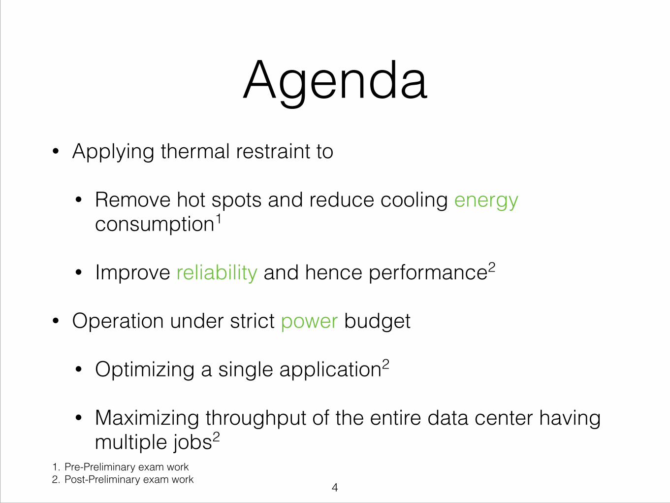
Agenda• Applying thermal restraint to

• Remove hot spots and reduce cooling energy consumption1

• Improve reliability and hence performance2

• Operation under strict power budget

• Optimizing a single application2

• Maximizing throughput of the entire data center having multiple jobs2

1. Pre-Preliminary exam work 2. Post-Preliminary exam work

!4

Thermal  Restraint!

!

Reducing  Cooling  Energy  Consumption

Publications• Osman Sarood, Phil Miller, Ehsan Totoni, and Laxmikant V. Kale. `Cool’ Load Balancing for High Performance

Computing Data Centers. IEEE Transactions on Computers, December 2012.

• Osman Sarood and Laxmikant V. Kale. Efficient `Cool Down’ of Parallel Applications. PASA 2012.

• Osman Sarood, and Laxmikant V. Kale. A `Cool’ Load Balancer for Parallel Applications. Supercomputing’11 (SC’11).

• Osman Sarood, Abhishek Gupta, and Laxmikant V. Kale. Temperature Aware Load Balancing for Parallel Application: Preliminary Work. HPPAC 2011. �5

Power Utilization Efficiency (PUE) in 2012

1. Matt Stansberry, Uptime Institute 2012 data center industry survey!6

PUEs for HPC Data Centers

• Most HPC data centers do not publish cooling costs

• PUE can change over time

Supercomputer PUE

Earth Simulator1 1.55

Tsubame2.02 1.31/1.46

ASC Purple1 1.67

Jaguar3 1.58

1. Wu-chen Feng, The Green500 List: Encouraging Sustainable Supercomputing 2. Satoshi Matsuoka, Power and Energy Aware Computing with Tsubame 2.0 and Beyond 3. Chung-Hsing Hsu et. al., The Energy Efficiency of the Jaguar Supercomputer!7

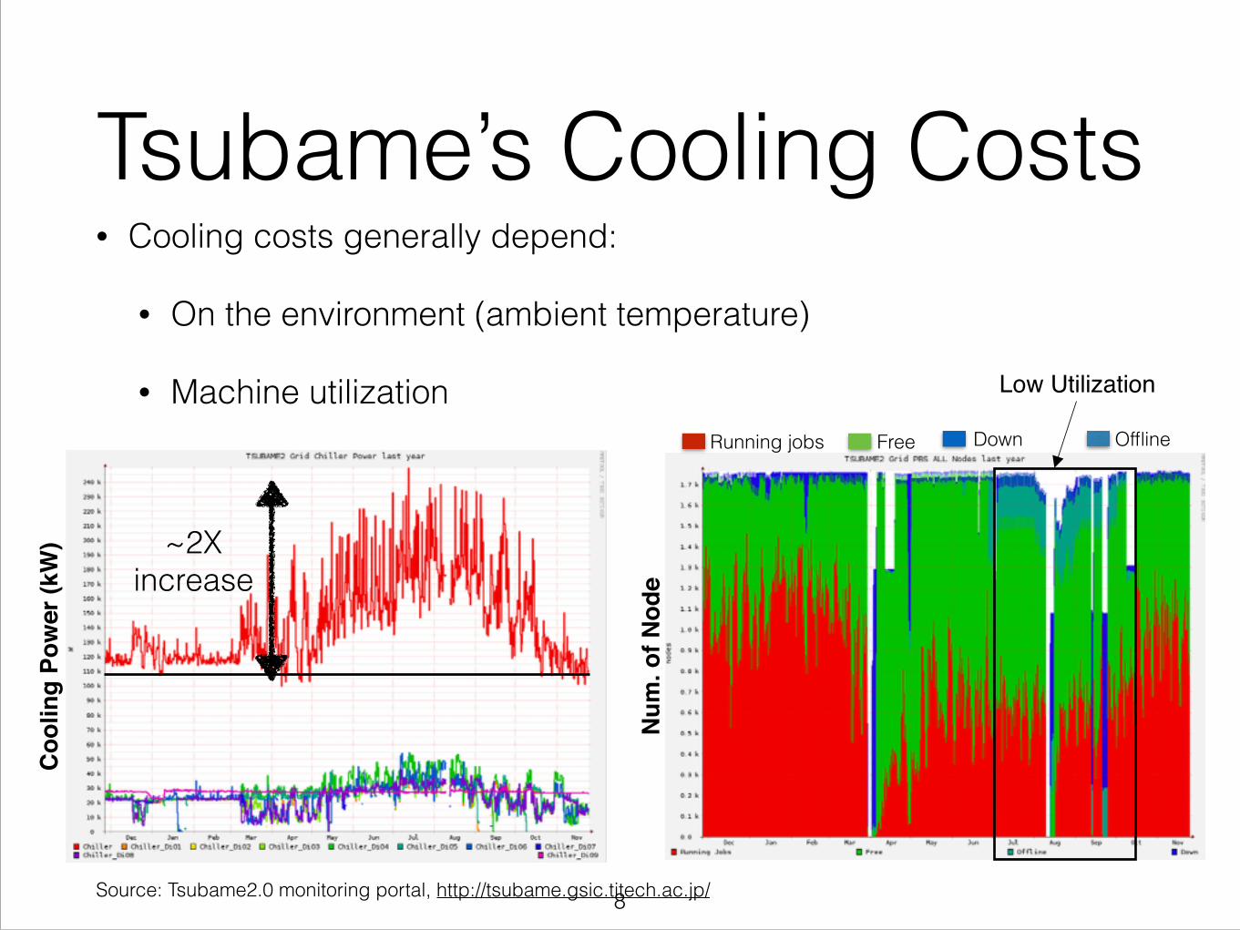
Tsubame’s Cooling Costs• Cooling costs generally depend:

• On the environment (ambient temperature)

• Machine utilization

~2X increase

Low Utilization

Source: Tsubame2.0 monitoring portal, http://tsubame.gsic.titech.ac.jp/

Coo

ling

Pow

er (k

W)

Num

. of N

ode

Running jobs Free Down Offline

!8

Hot spots

1. Dale Sartor, General Recommendations for High Performance Computing Data Center Energy Management Dashboard Display (IPDPSW 2013)

HPC Cluster Temperature Map, Building 50B room 1275, LBNL

Can software do anything to reduce cooling energy and

formation of hot spots?

!9

`Cool’  Load  Balancer

• Uses  Dynamic  Voltage  and  Frequency  Scaling  (DVFS)  • Specify  temperature  range  and  sampling  interval  • Runtime  system  periodically  checks  processor  temperatures  

• Scale  down/up  frequency  (by  one  level)  if  temperature  exceeds/below  maximum  threshold  at  each  decision  time  

• Transfer  tasks  from  slow  processors  to  faster  ones  • Using  Charm++  adaptive  runtime  system  • Details  in  dissertation

�10

Average  Core  Temperatures  in  Check

• Avg.  core  temperature  within  2  C  range  • Can  handle  applications  having  different  temperature  gradients

�11

CRAC  set-­‐point  =  25.6C          Temperature  range:  47C-­‐49C

Execution Time (seconds)

(32 nodes)

Benefits  of  `Cool’  Load  Balancer

�12

Normalization w.r.t run without temperature restraint

Thermal  Restraint!

!

Improving  Reliability  and  Performance

Publications• Osman Sarood, Esteban Meneses, and Laxmikant V. Kale. A `Cool’ Way of Improving the Reliability of HPC Machines.

Supercomputing’13 (SC’13).

Post-Preliminary Exam Work

�13

Fault tolerance in present day supercomputers

• Earlier studies point to per socket Mean Time Between Failures (MTBF) of 5 years - 50 years

• More than 20% of computing resources are wasted due to failures and recovery in a large HPC center1

• Exascale machine with 200,000 sockets is predicted to waste more than 89% time in failure/recovery2

1. Ricardo Bianchini et. al., System Resilience at Extreme Scale, White paper 2. Kurt Ferreira et. al., Evaluating the Viability of Process Replication Reliability for Exascale Systems, Supercomputing’11 !14

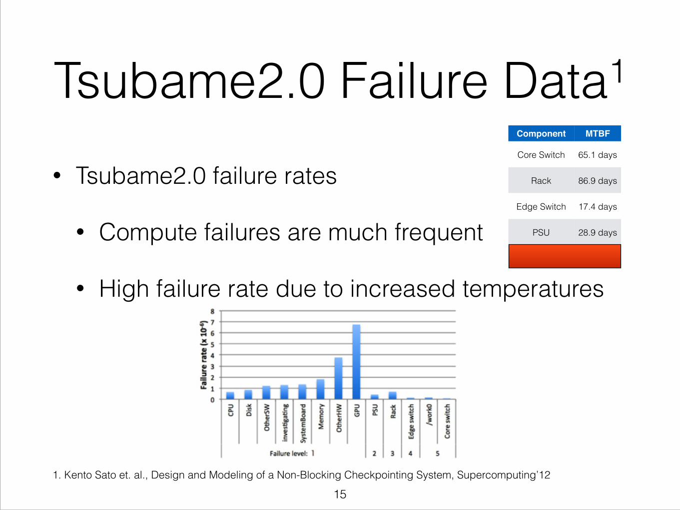
Tsubame2.0 Failure Data1

• Tsubame2.0 failure rates

• Compute failures are much frequent

• High failure rate due to increased temperatures

!

Component MTBF

Core Switch 65.1 days

Rack 86.9 days

Edge Switch 17.4 days

PSU 28.9 days

Compute Node 15.8 hours

1. Kento Sato et. al., Design and Modeling of a Non-Blocking Checkpointing System, Supercomputing’12

!15

Tsubame Fault Analysis

Jan Feb Mar Apr May Jun Jul Aug Sep Oct Nov0

1

2

3

4

5

6

Avg.

Fau

lts p

er d

ay

4.3

3.1

1.9

Tokyo Average Temperature~2X

increase!

Coo

ling

Pow

er

Num

. of N

odes

Source: Tsubame2.0 monitoring portal, http://tsubame.gsic.titech.ac.jp/

Running jobs Free Down Offline

!16

CPU Temperature and MTBF• 10 degree rule: MTBF halves (failure rate doubles) for

every 10C increase in temperature1 • MTBF (m) can be modeled as: !

where ‘A’, ‘b’ are constants and ’T’ is processor

temperature • A single failure can cause the entire machine to fail,

hence MTBF for the entire machine (M) is defined as: !!

1. Wu-Chun Feng, Making a Case for Efficient Supercomputing, New York, NY, USA

!17

Related Work

• Most earlier research focusses on improving fault tolerance protocol (dealing efficiently with faults)

• Our work focusses on increasing the MTBF (reducing the occurrence of faults)

• Our work can be combined with any fault tolerance protocol

!18

Distribution of Processor Temperature

• 5-point stencil application (Wave2D from Charm++ suite)

• 32 nodes of our Energy Cluster1

• Cool processor mean: 59C, std deviation: 2.17C

!

!

!

1. Thanks to Prof. Tarek Abdelzaher for allowing us to use the Energy Cluster !19

Estimated MTBF - No Temperature Restraint

• Using observed max temperature data and per-socket MTBF of 10 years (cool processor mean: 59C, std deviation: 2.17C)

• Formula for M:

50 55 60 65 70 75 8020

25

30

35

40

45

50

55

60

Maximum allowed temperature ( °C)

MT

BF

of

32

−n

od

e c

lust

er

(da

ys)

45 50 55 60 65 70 75 80 850

1

2

3

4

5

6

7

Nu

mb

er

of

pro

cess

ors

Processor temperature ( °C)

Cool ProcessorsHot Processors

!20

Estimated MTBF - Removing Hot Spot

• Using measured max temperature data for cool processors and 59C (same as average temperature for cool processors) for hot processors

50 55 60 65 70 75 8020

25

30

35

40

45

50

55

60

Maximum allowed temperature ( °C)

MT

BF

of

32

−n

od

e c

lust

er

(da

ys)

45 50 55 60 65 70 75 80 850

1

2

3

4

5

6

7

Nu

mb

er

of

pro

cess

ors

Processor temperature ( °C)

Cool ProcessorsHot Processors

!21

Estimated MTBF - Temperature Restraint

• Using randomly generated temperature data with mean: 50C and std deviation: 2.17C (same as cool processors from the experiment)

50 55 60 65 70 75 8020

25

30

35

40

45

50

55

60

Maximum allowed temperature ( °C)

MT

BF

of 32−

node c

lust

er

(days

)

45 50 55 60 65 70 75 80 850

1

2

3

4

5

6

7

Num

ber

of pro

cess

ors

Processor temperature ( °C)

Cool ProcessorsHot Processors

!22

Recap• Restraining temperature can improve the estimated

MTBF of our Energy Cluster

• Originally (No temperature control): 24 days

• Removing hot spots: 32 days

• Restraining temperature (mean 50C): 58 days

• How can we restrain processor temperature?

• Dynamic Voltage and Frequency Scaling (DVFS)5?5. Reduces both voltage and frequency which reduces power consumption resulting in temperature to fall

!23

Restraining Processor Temperature

• Extension of `Cool’ Load Balancer

• Specify temperature threshold and sampling interval

• Runtime system periodically checks processor temperature

• Scale down/up frequency (by one level) if temperature exceeds/below maximum threshold at each decision time

• Transfer tasks from slow processors to faster ones

• Extended by making it communication aware (details in paper):

• Select objects (for migration) based on the amount of communication it does with other processors

!24

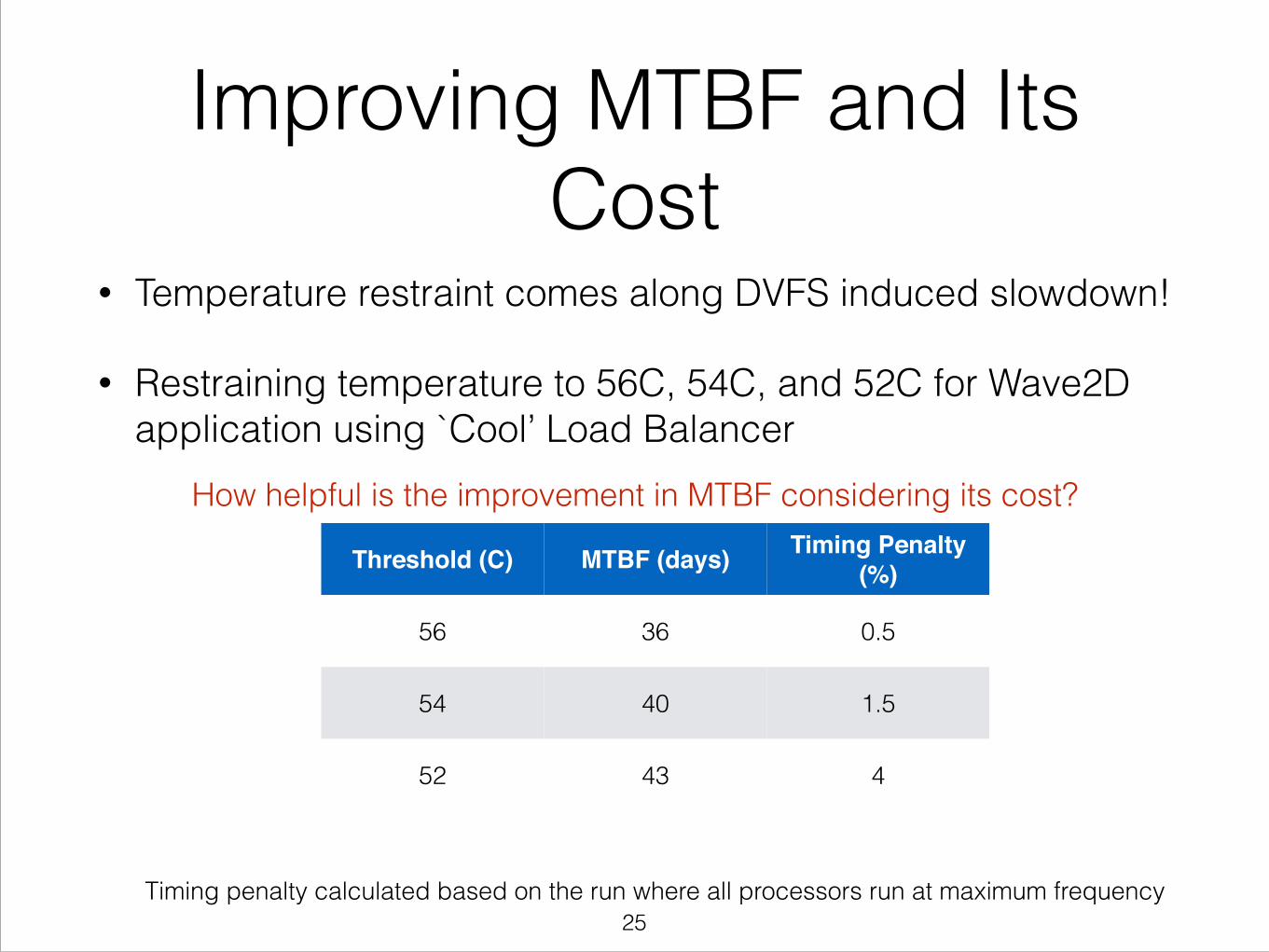
Improving MTBF and Its Cost

• Temperature restraint comes along DVFS induced slowdown!

• Restraining temperature to 56C, 54C, and 52C for Wave2D application using `Cool’ Load Balancer

Timing penalty calculated based on the run where all processors run at maximum frequency

Threshold (C) MTBF (days) Timing Penalty (%)

56 36 0.5

54 40 1.5

52 43 4

How helpful is the improvement in MTBF considering its cost?

!25

Performance Model

• Execution time (T): sum of useful work, check pointing time, recovery time and restart time

• Temperature restraint:

• decreases MTBF which in turn decreases check pointing, recovery, and restart times

• increases time taken by useful work

!26

Performance ModelSymbol Description

T Total execution time

W Useful work

Check point period

δ check point timeR Restart timeµ slowdown

1

1. J. T. Daly, A higher order estimate of the optimum checkpoint interval for restart dumps !27

Model Validation• Experiments on 32-nodes of Energy Cluster

• To emulate the number of failures in a 700K socket machine, we utilize a scaled down value of MTBF (4 hours per socket)

• Inject random faults based on estimated MTBF values using ‘kill -9’ command

• Three applications:

• Jacobi2D: 5 point-stencil

• LULESH: Livermore Unstructured Lagrangian Explicit Shock Hydrodynamics

• Wave2D: finite difference for pressure propagation

!28

Model Validation• Baseline experiments:

• Without temperature restraint

• MTBF based on actual temperature data from experiment

• Temperature restrained experiments:

• MTBF calculated using the max allowed temperature

!29

Reduction in Execution Time• Each experiment was longer than 1 hour having at

least 40 faults

• Inverted-U curve points towards a tradeoff between timing penalty and improvement in MTBF

Reduction in time calculated compared to baseline case with no temperature control

Times improvement in MTBF over baseline

!30

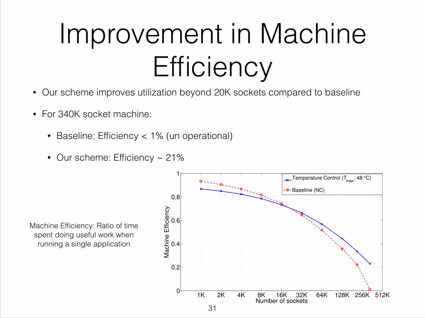
Improvement in Machine Efficiency

• Our scheme improves utilization beyond 20K sockets compared to baseline

• For 340K socket machine:

• Baseline: Efficiency < 1% (un operational)

• Our scheme: Efficiency ~ 21%

1K 2K 4K 8K 16K 32K 64K 128K 256K 512K0

0.2

0.4

0.6

0.8

1

Number of sockets

Ma

chin

e E

ffic

ien

cy

Temperature Control (Tmax

: 48 °C)

Baseline (NC)

Machine Efficiency: Ratio of time spent doing useful work when running a single application

!31

Predictions for Larger Machines

• Per-socket MTBF of 10 years

• Optimum temperature thresholds

Improvement in MTBF compared to baseline

Reduction in time calculated compared to baseline case with no temperature control !32

Power  Constraint!

!

Improving  Performance  of  a  Single  Application

�33

Publications• Osman Sarood, Akhil Langer, Laxmikant V. Kale, Barry Rountree, and Bronis de Supinski. Optimizing Power Allocation to CPU

and Memory Subsystems in Overprovisioned HPC Systems. IEEE Cluster 2013.

What’s the Problem?Exascale in

20MW!

Power consumption for Top500

Make the best use of each Watt of power!

!34

Overprovisioned Systems1

• What we currently do:

• Assume each node consumes Thermal Design Point (TDP) power

• What we should do (overprovisioning):

• Limit power of each node and use more nodes than a conventional data center

• Overprovisioned system: You can’t run all nodes at max power simultaneously

1. Patki et. al., Exploring hardware overprovisioning in power-constrained, high performance computing, ICS 2013

Example!10 nodes @ 100 W (TDP)

20 nodes @ 50 W

!35

Where Does Power Go?• Power distribution for BG/Q

processor on Mira

• CPU/Memory account for over 76% power

• No good mechanism of controlling other power domains

1. Pie Chart: Sean Wallace, Measuring Power Consumption on IBM Blue Gene/Q

Small with small variation over time

!36

Power  Capping  -­‐  RAPL

• Running  Average  Power  Limit  (RAPL)  library  • Uses  Machine  Specific  Registers  (MSRs)  to:  – measure  CPU/Memory  power    – set  CPU/memory  power  caps  

• Can  report  CPU/memory  power  consumption  at  millisecond  granularity

�37

Problem  Statement

Optimize  the  numbers  of  nodes  (n  ),  the  CPU  power  level  (pc)  and  memory  power  level  (pm  )  that  minimizes  execution  time  (t  )  of  an  application  under  a  strict  power  budget  (P  ),  on  a  high  performance  computation  cluster  with  p_b    as  the  base  power  per  node  i.e.  determine  the  best  configuration    (n  x  {pc,  pm})

�38

Applications  and  Testbed

• Applications  • Wave2D:  computation-­‐intensive  finite  differencing  application  

• LeanMD:  molecular  dynamics  simulation  program  • LULESH:  Hydrodynamics  code  

• Power  Cluster  • 20  nodes  of  Intel  Xeon  E5-­‐2620  • Power  capping  range:  

• CPU:  25-­‐95  W  • Memory:  8-­‐38W

�39

Profiling  Using  RAPL       Profile  configurations  (n  x  pc,  pm  )

n:  Num  of  nodes  pc:  CPU  power  cap  pm:  Memory  power  cap  !n:  {5,12,20}  pb:  {28,32,36,44,50,55}  pm:  {8,10,18}  pb:  38  Tot.  power  =    n  *  (pc  +  pm  +  pb)  

Profile  for  

(20x32,10)  

(12x44,18)  

(5x55,18)  

�40

Can  We  Do  Better?

!

• More  profiling  (Expensive!)  • Using  interpolation  to  estimate  all  possible  combinations

�41

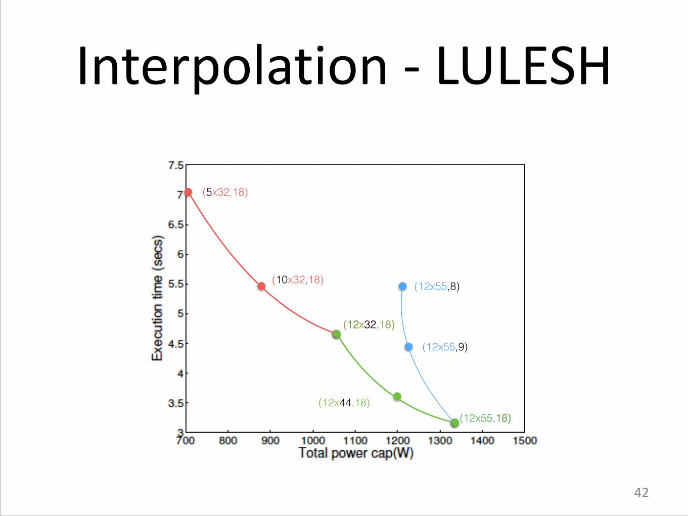
Interpolation  -­‐  LULESH

(12x55,8)

(12x55,9)

(12x55,18)(12x44,18)

(12x55,18)

(12x32,18)

(10x32,18)

(5x32,18)

(12x32,18)

�42

Evaluation

• Baseline  configuration  (no  power  capping):  !

!

!

• Compare:  – Profiling  scheme:  Only  the  profile  data  – Interpolation  Estimate:  The  estimated  execution  time  using  interpolation  scheme  

– Observed:  Observed  execution  for  the  best  configurations

�43

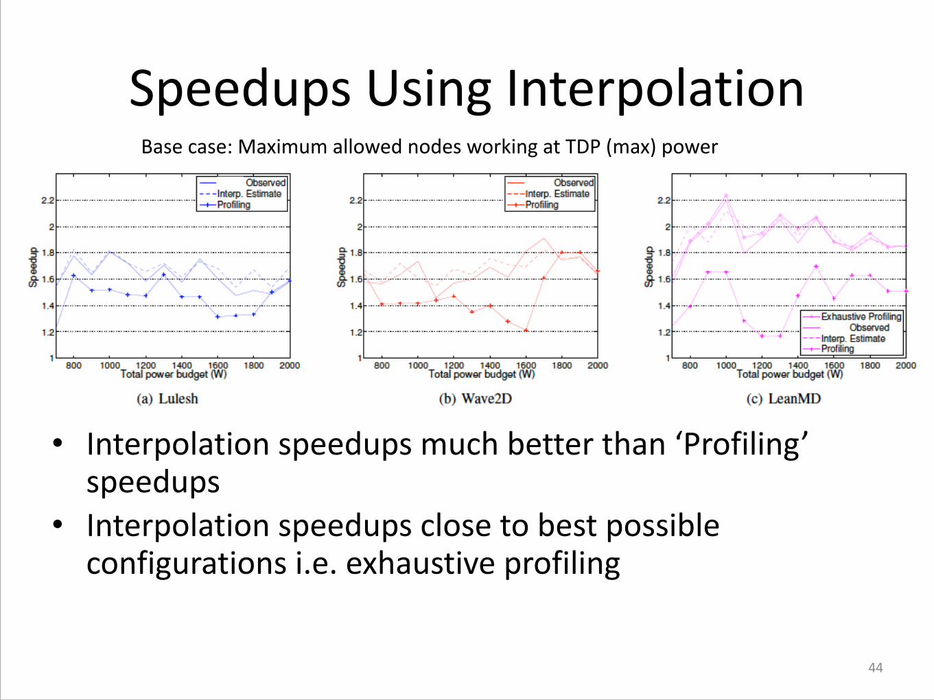
Speedups  Using  Interpolation

• Interpolation  speedups  much  better  than  ‘Profiling’  speedups  

• Interpolation  speedups  close  to  best  possible  configurations  i.e.  exhaustive  profiling

Base  case:  Maximum  allowed  nodes  working  at  TDP  (max)  power

�44

Optimal CPU/Memory PowersCPU/Memory  powers  for  different  power  budgets:  • M:  observed  power  using  our  scheme  • B:  observed  power  using  the  baseline

�45

Save power to add more nodes (Speedup~2X)

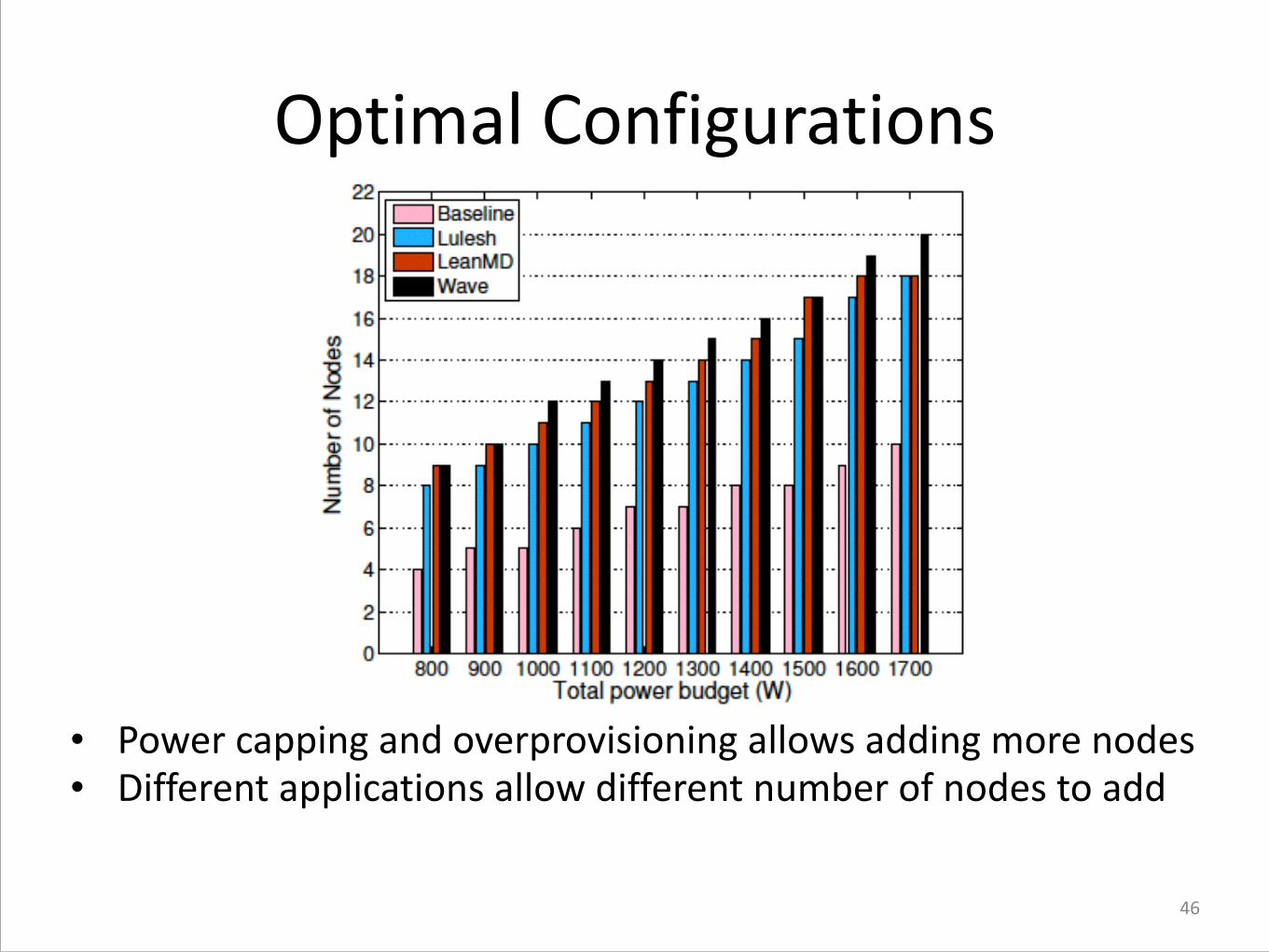
Optimal  Configurations

• Power  capping  and  overprovisioning  allows  adding  more  nodes  • Different  applications  allow  different  number  of  nodes  to  add

�46

Power ConstraintOptimizing Data Center Throughput having Multiple Jobs

Publications• Osman Sarood, Akhil Langer, Abhishek Gupta, Laxmikant Kale. Maximizing Throughput of Overprovisioned HPC Data Centers

Under a Strict Power Budget. IPDPS 2014 (in submission).

!47

Data Center Capabilities

• Overprovisioned data center

• CPU power capping (using RAPL)

• Moldable and malleable jobs

!48

Moldability and MalleabilityMoldable jobs

• Can execute on any number of nodes within a specified range

• Once scheduled, number of nodes can not change

Malleable jobs:

• Can execute on any number of nodes within a range

• Number of nodes can change during runtime

• Shrink: reduce the number of allocated nodes

• Expand: increase the number of allocated nodes

!49

The Multiple Jobs Problem

Given a set of jobs and a total power budget, determine:

• subset of jobs to execute

• resource combination (n x pc) for each job

such that the throughput of an overprovisioned system is maximized

!50

Framework

Scheduler

`Job  Arrives Job  Ends

Schedule  Jobs  (ILP)

Queue

Launch  Jobs/  Shrink-­‐Expand

Ensure  Power  Cap

Execution  framework

Triggers

Strong  Scaling  Power  Aware  Module

Resource  Manager

!51

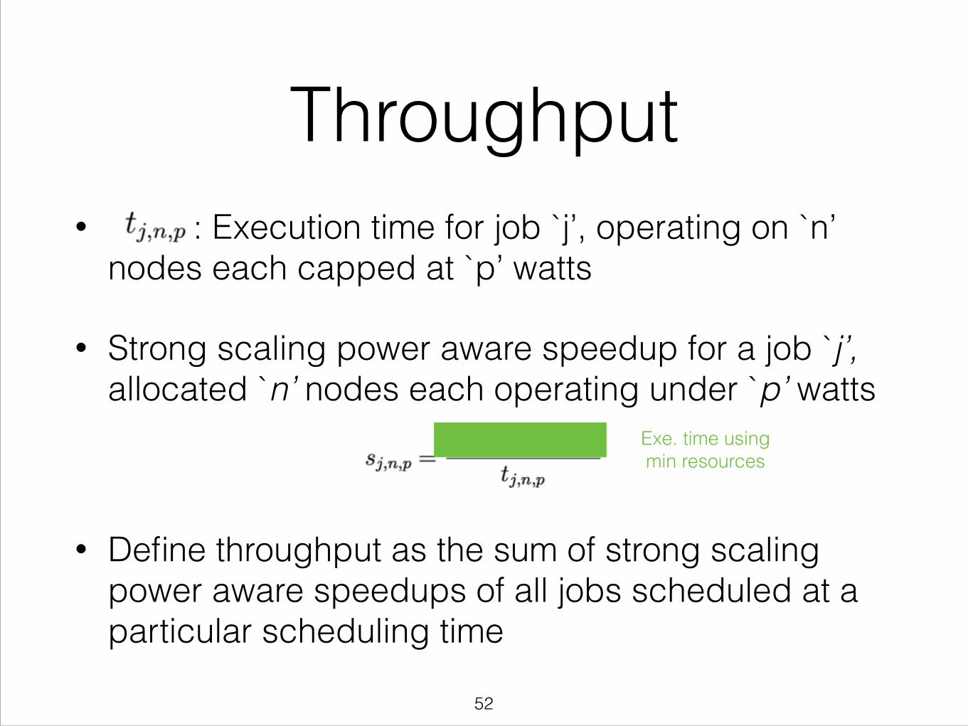
Throughput• : Execution time for job `j’, operating on `n’

nodes each capped at `p’ watts

• Strong scaling power aware speedup for a job `j’, allocated `n’ nodes each operating under `p’ watts

!

• Define throughput as the sum of strong scaling power aware speedups of all jobs scheduled at a particular scheduling time

Exe. time using min resources

!52

Scheduling Policy (ILP)Starvation!

!53

Making the Objective Function Fair

• Assigning a weight to each job `j’

!

• : arrival time of job `j’

• : current time at present scheduling decision

• : remaining time for job ‘j ’ executing at minimum power operating at lowest power level

Time elapsed since arrival

Remaining time using min resources Extent of fairness

!54

Objective Function

Scheduler

Framework

Job  Arrives Job  Ends

Schedule  Jobs  (ILP)

Queue

Launch  Jobs/  Shrink-­‐Expand

Ensure  Power  Cap

Execution  framework

Triggers

Strong  Scaling  Power  Aware  Module

Resource  Manager

Model

Job  Characteristics  Database

Profile  Table

!55

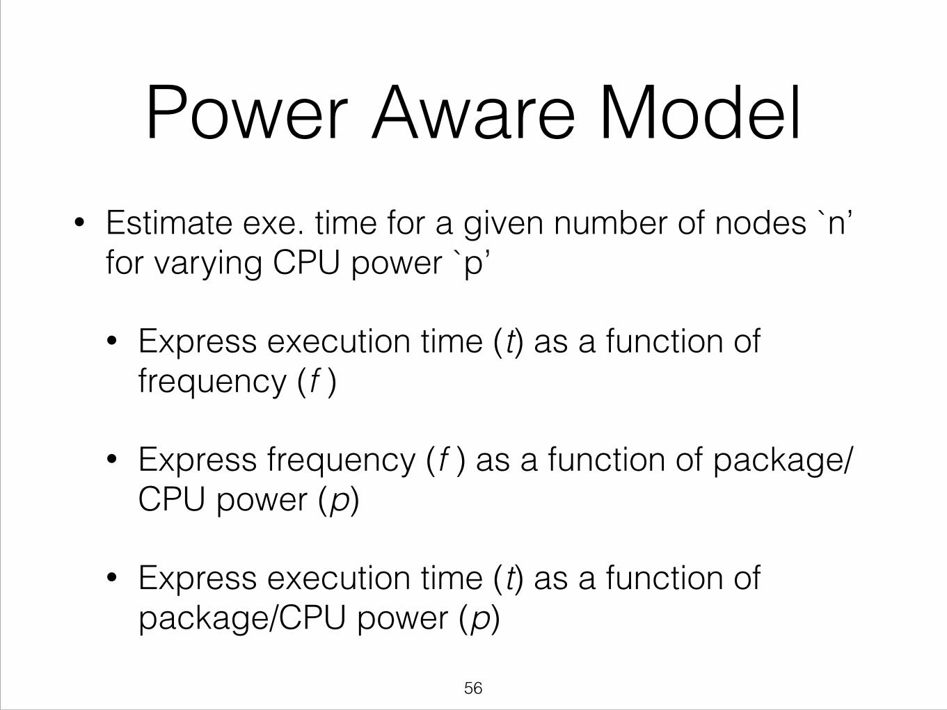
Power Aware Model• Estimate exe. time for a given number of nodes `n’

for varying CPU power `p’

• Express execution time (t) as a function of frequency (f )

• Express frequency (f ) as a function of package/CPU power (p)

• Express execution time (t) as a function of package/CPU power (p)

!56

Power Aware Strong Scaling

• Extend Downey’s strong scaling model

• Build a power aware speedup model

• Combine strong scaling model with power aware model

• Given a number of nodes `n’ and a power cap for each node `p’, our model estimates execution time

!57

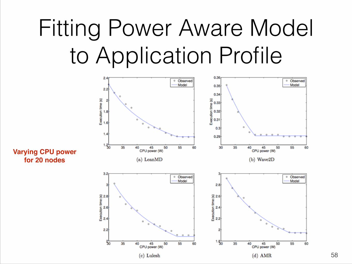
Fitting Power Aware Model to Application Profile

Varying CPU power for 20 nodes

!58

Power Aware Speedup and Parameters

Estimated Parameters

Speedups based on execution time at lowest CPU power

!59

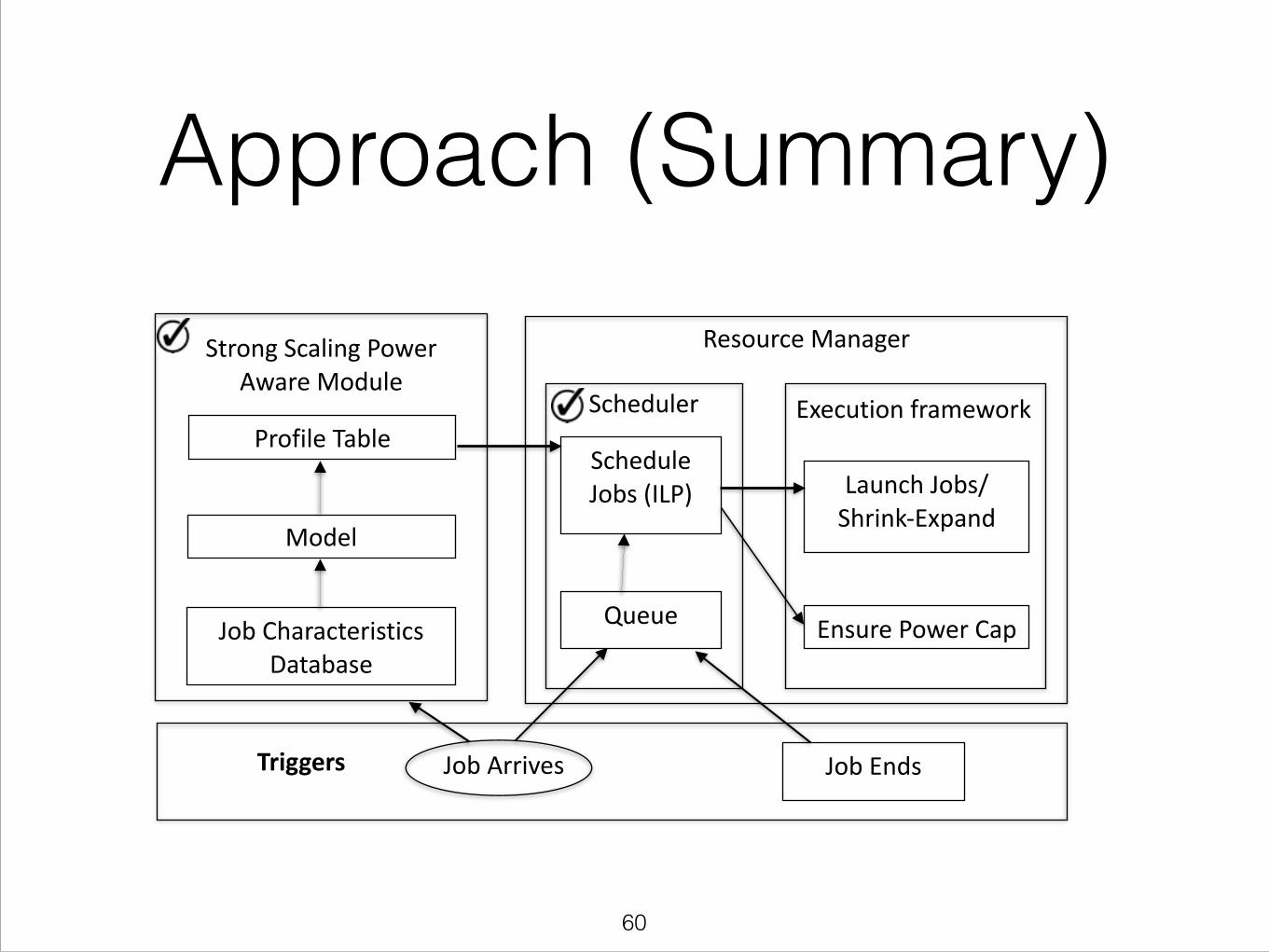
Scheduler

Approach (Summary)

Job  Arrives Job  Ends

Schedule  Jobs  (ILP)

Queue

Launch  Jobs/  Shrink-­‐Expand

Ensure  Power  Cap

Execution  framework

Triggers

Strong  Scaling  Power  Aware  Module

Resource  Manager

Model

Job  Characteristics  Database

Profile  Table

!60

Experimental Setup• Comparison with baseline policy of SLURM

• Using Intrepid trace logs (ANL, 40,960 nodes, 163,840 cores)

• 3 data sets each containing 1000 jobs

• Power characteristics: randomly generated

• Includes data transfer and boot time cost for shrink/expand

!61

Experiments: Power Budget (4.75 MW)

• noSE: Our scheduling policy with only moldable jobs. CPU power <=60W, memory power 18W and base power 38W, nodes > 40,960 nodes

• Baseline policy/SLURM: using 40,960 nodes operating at CPU power 60W, memory power 18W, and base power 38W. SLURM Simulator1

• wiSE: Our scheduling policy with both moldable jobs and malleable jobs i.e. shrink/expand. CPU power <=60W, memory power 18W and base power 38W, nodes > 40,960 nodes

1. A. Lucero, SLURM Simulator !62

Metrics

• Response time: Time interval between arrival and start of execution

• Completion time: response time + execution time

• Max completion time: Largest completion time for any job in the set

!63

Changing Workload Intensity ( )

• Multiplying arrival time of each job in a set with

• Compressing data set by a factor

• Impact of increasing job arrival rate

!64

Speedup

wiSE better than noSE

Increasing job arrival increases speedup

Not enough jobs: Low speedups

Speedup compared to baseline SLURM !65

Comparison With Power Capped SLURM

• Its not just overprovisioning!

• wiSE compared to a power capped SLURM policy using over provisioning for Set2

• Cap CPU powers below 60W to benefit from overprovisioning

!66

Tradeoff Between Fairness and Throughput

Aver

age

Com

plet

ion

Tim

e (s

)

!67

Varying Number of Power Levels

Increasing number of power levels:

• Increase cost of solving ILP

• Improve the average or max completion time

Aver

age

Com

plet

ion

Tim

e (s

)

!68

Major Contributions• Use of DVFS to reduce cooling energy consumption

• Cooling energy savings of up to 63% with timing penalty between 2-23%

• Impact of processor temperature on reliability of an HPC machine

• Increase MTBF by as much as 2.3X

• Improve machine efficiency by increasing MTBF

• Enables machine to operate with 21% efficiency for 340K socket machine (<1% for baseline)

• Use of CPU and memory power capping to improve application performance

• Speedup of up to 2.2X compared to case that doesn’t use power capping

• Power aware scheduling to improve data center throughput

• Both our power aware scheduling schemes achieve speedups up to 4.5X compared to baseline SLURM

• Power aware modeling to estimate an application’s power-sensitivity

!69

Publications (related)• Osman Sarood, Akhil Langer, Abhishek Gupta, Laxmikant Kale. Maximizing Throughput of Overprovisioned HPC Data

Centers Under a Strict Power Budget. IPDPS 2014 (in submission).

• Esteban Meneses, Osman Sarood, and Laxmikant V. Kale. Energy Profile of Rollback-Recovery Strategies in High Performance Computing. Elsevier - Parallel Computing (invited paper - in submission).

• Osman Sarood, Esteban Meneses, and Laxmikant V. Kale. A `Cool’ Way of Improving the Reliability of HPC Machines. Supercomputing’13 (SC’13).

• Osman Sarood, Akhil Langer, Laxmikant V. Kale, Barry Rountree, and Bronis de Supinski. Optimizing Power Allocation to CPU and Memory Subsystems in Overprovisioned HPC Systems. IEEE Cluster 2013.

• Harshitha Menon, Bilge Acun, Simon Garcia de Gonzalo, Osman Sarood, and Laxmikant V. Kale. Thermal Aware Automated Load Balancing for HPC Applications. IEEE Cluster.

• Esteban Meneses, Osman Sarood and Laxmikant V. Kale. Assessing Energy Efficiency of Fault Tolerance Protocols for HPC Systems. IEEE SBAC-PAD 2012. Best Paper Award.

• Osman Sarood, Phil Miller, Ehsan Totoni, and Laxmikant V. Kale. `Cool’ Load Balancing for High Performance Computing Data Centers. IEEE Transactions on Computers, December 2012.

• Osman Sarood and Laxmikant V. Kale. Efficient `Cool Down’ of Parallel Applications. PASA 2012.

• Osman Sarood, and Laxmikant V. Kale. A `Cool’ Load Balancer for Parallel Applications. Supercomputing’11 (SC’11).

• Osman Sarood, Abhishek Gupta, and Laxmikant V. Kale. Temperature Aware Load Balancing for Parallel Application: Preliminary Work. HPPAC 2011.

!70

Thank You!

!71

Varying  Amount  of  Profile  Data

• Observed  speedups  using  different  amount  of  profile  data  • 112  points  suffice  to  give  reasonable  speedup  

�72

Blue Waters Cooling

63F$62F$

69F$69F$

70F$69F$

68F$68F$

65F$65F$

63F$64F$

63F$63F$

Row$1$

Row$7$

Blue Waters Inlet Water Temperature for Different Rows

!73