performance of movable-head disk storage devices
TRANSCRIPT

Performance of Movable-Head Disk Storage Devices
C. C. G O T L 1 E B A N D G . t I . M A C E W E N
Univer~,:ity of Toronto, Toronto, Ontario, Canada
ABSTRACT. A queueing model of movable-head disk storage systems is developed so that the per- formance, as measured by the mean response time, can be calculated. Queue scheduling algorithms which improve the performance are considered. Single-module disk systems are analyzed, incor- porating the SCAN scheduling algorithm suggested by Denning so that comparisons with the FIFO algorithm are possible. This analysis is extended to multimodule systems whereby tables of approxi- mate glean response values time can be calculated over system parameters describing equipment characteristics, equipment configuration, system loading, file organization, and scheduling algorithm (SCAN or FIFO). The use of such tables is discussed and the applicability of the analysis to a re- cently marketed disk is noted.
KEY WORDS AND PHRASES: secondary storage, disk storage, queueing model, queueing analysis, scheduling, file organization, input/output, state-dependent queues, imbedded Markov chain, steady state analysis, system design
CR CATEGORIES: 4.3, 4.41, 6.2, 6.35
1. Introduction
Movable-head disk storage devices (simply called disks in the remainder of the paper) are commonly used for secondary storage, that is, for the storage of programs and data that are required lelatively infrequently but which may be needed at any time. They are attractive because of their size, speed, and cost, as compared with alternatives such as ma~metic tape or card devices. Many general purpose computing systems, as well as special purpose systems such as message switching systems, reservation systems, and information retrieval systems, use disks.
The overall processing efficiency and performance of computer systems depend criti- cally on the response time of secondary storage [2, 3], the time from the initiation of a data transfer request to the completion of the transfer operation. Disk devices have been evaluated from varying viewpoints, and with varying techniques [4-9]; the performance measure chosen reflects the approach taken in the evaluation. Fife and Smith [4] chose the performance measure of maximum mean data transfer rate to analyze multichannel disk configurations. This led them to assume full load conditions (that is, the queue of requests is never empty) in their analysis. A more common measure is mean response time [5-8] since it does not imply any such restriction.
Different ways of scheduling data transfer requests have been suggested [6, 8, 9] as a means of reducing mean response time. In particular, two scheduling algorithms are simple enough and yet potentially effective enough to be considered as alternatives to the FIFO (first-in-first-out) queue discipline which is generally adopted. The first,
Copyright © 1973, Association for Computing Machinery, Inc. General permission to republish, but not for profit, all or part of this material is granted provided that ACM's copyright notice is given and that reference is made to the publication, to its date of issue, and to the fact that reprinting privileges were granted by permission of the Association for Computing Machinery. Authors' present addresses: C. C. Gotlieb, Department of Computer Science, University of Toronto, Toronto MSS 1A7, Ontario, Canada; G. H. MacEwen, Department of Computing and Information Science, Queen's University, Kingston, Ontario, Canada. This paper is based on the Ph.D. thesis of G. H. MacEwen [1].
Journal of the Association for Computing Machinery, Vol. 20, No. 4, October 1973, pp. 604-623.

Performance of Movable-Head Disk Storage Devices 605
SCAN, 1 operates by sweeping the access arm in one direction across the disk, always moving from the cylinder 2 last involved in a da ta transfer to the closest cylinder (in the direction the arm is being swept) for which a da ta transfer request is waiting in the queue; if no such request exists, the direction of sweeping is reversed. The second schedul- ing algorithm, SSTF (shortest-seek-time-first), operates by simply moving the arm to the closest cylinder for which a data transfer request is waiting in t h e queue, regard- less of the direction.
Queueing theory is useful to represent the congestion of da ta transfer requests occur- ring in a heavily loaded disk system; no queueing model for multimodule 3 movable-head disks has previously been developed which incorporates a scheduling algorithm other than FIFO. In this paper, disk storage performance is analyzed by using queueing theory to calculate the mean response time over a range of parameters which determine the characteristics of the disk storage system.
A queueing model of a single-channel disk system is first developed so tha t mean re- sponse time, E[T], can be calculated as a function of:
(a) equipment characteristics; (b) equipment configuration (the number of disk modules is not restricted to large
values, as in [7], but is variable, as in [5], up to certain limits imposed by practical rather than theoretical reasons);
(c) file organizat ion--block lengths are taken to be uniformly distributed over a fixed range and Seaman's method [5] of channel act ivi ty analysis is generalized to incorporate this distribution;
(d) system loading; (e) request scheduling a lgor i thm--SCAN or FIFO. SCAN scheduling,rather t hanSSTF ,
is chosen for detailcd at tention on the basis of system equity; SSTF discriminates against requests accessing certain cylinders. Preliminary simulations showed tha t although SSTF yields lower values of E[T] than SCAN, most of the improvement over F I F O gained with SSTF is obtainable with SCAN.
E[T] is not obtained in a closed form, but a procedure is given whereby tables of ap- proximate values of E[T] are calculated and typical curves are produced. General con- clusions about disk systems, based on calculated results, are drawn. In addition, the use of such tables of E[T] for engineering design is discussed. Finally, the relevance of the work to newer types of disks is discussed.
I t should be added tha t a mathematical analysis of an idealized single-module disk model has recently been described [23]. This analysis examines two different versions of SCAN: one in which requests arriving during a sweep are serviced in the following sweep, and one in which each sweep is performed in the same direction.
2. The Disk Model
The type of device under study is typified by the IBM 2314 [10] which is used for illustra- tion in the remainder of this paper. The timing sequence occurring as a da ta transfer request 4 is satisfied, if software and hardware overhead times are ignored, is described by Figure 1. The data channel is needed to initiate arm motion. I t can be shown [1] tha t the time required to wait for the channel to become free to initiate arm motion may be ignored since its mean value is small compared to the times shown in Figure 1.
The disk model is a set of queues as shown in Figure 2. Each distinct module queue is considered, since one objective is to determine the response time for a varying number
1 SCAN, as described here, is called LOOK in [8]. A cylinder is a set of tracks (one or more per disk surface) written onto while the access arm is
stationary at one of a set of discrete mechanical positions to which it can be moved. a A disk module contains one independently movable access arm.
A request, generated by any process in the system, is received by the Input/Output Supervisor which manages the data transfer.

~ 0 6 C. C. GOTLIEB AND G. H. MAcEWEN
Module queueing
time
I Module | • queue
s~ce !
Arm Channel motion queueing time _ time _
m "W -
Channel queue service time
Rotational i Transfer delay time
r V
• Channel busy
Module busy
Response time
FwG. 1. Timing diagram for disk model
Mean request rate
~/M I/M ~/M
M MODULE QUEUES
L[ CHISEL
I QUEUE
FIo. 2. Queueing model of single-channel disk
of modules. Arm motion time constitutes the module queue service time, and rotational delay plus block transfer t ime constitute the channel queue service time. 5 Note from Figure 1 that a module queue server remains busy as long as the request it last served occupies the channel queue. It is necessary, therefore, to specify that a module queue server remains busy after serving a request until that request has completed its channel service time.
The following assumptions complete the specification of the model. (a) Requests are independent and arrive randomly in time at the queues, each module
being equally likely to be addressed. The interarrival distribution function is given by
I1 - e -~ , t > 0, F~(t) = O, t < O,
where X is the mean request rate. The interarrival t ime distribution of requests to each module queue is also exponential with a mean request rate of k / M .
Blocks of data are recorded on circular tracks which rotate under read/write heads mounted on the access arm.

Performance of Movable-Head Disk Storage Devices 607
Time in
milliseconds
120
80,
40'
A p p r o x i m a t V ~
ae
• A c t u a l
slope = a
l / I I I I
40 80 120 160 C=200
Cylinders travelled
FIG. 3. IBM 2314 arm movement time
The exponential distribution is chosen for two reasons. First, the assumption of random arrivals is the safest one in the absence of other information about the interarrival dis- tribution. (Information about arrival distributions of disk requests in actual systems is needed, and could be provided by a study analogous to that of Fuchs and Jackson [11] on computer communications traffic.) Second, a large body of useful queueing theory be- comes available if one assumes an exponential distribution for interarrival times.
(b) The plot of arm motion distance against time is approximated by a straight line as shown in Figure 3. C is the number of cylinders and a and b are determined by fitting a straight line to the actual module characteristics, shown for the 2314.
(c) The channel queue scheduling algorithm is FIFO. (d) The channel queue service time consists of the rotational delay plus the transfer
time. The distribution of this random variable depends on the manner in which blocks are stored on the disk and the lengths of the blocks. (For example, some disks store blocks on fixed length physical records called sectors. The waiting time for a randomly chosen sector to rotate under the heads is uniformly distributed between 0 and r, the total time to complete one full rotation. If block lengths, hence block transfer times, are uniformly distributed between 0 and B, the channel queue service time to transfer a randomly chosen block is given by a triangular distribution, nonzero between 0 and r + B. ) To ap- proximate a variety of situations and for ease of analysis, channel queue service time is taken to be uniformly distributed between 0 and r -4- B. Tile service time distribution function is, therefore,
t 0, t < 0, Fc(t) = t/R, 0_< t < R,
(1, t > R, whereR = r T B .
(e) Module queue scheduling is either FIFO or SCAN. (f) Cylinder addresses, which have integer values between 1 and C, are approxi-
mated by real numbers in the interval (0, C). A cylinder address is associated with each request. Each address is a random variable 8 z distributed according to a given continuous probability density function, fz (z). The function fz (z) is included in the model in an at- tempt to take into account the way in which disk storage space is allocated in a given
6 Boldface letters denote random variables.

6 0 8 c . c . GOTLIEB AND G. H. MAcEWEN
application. For this work, f , (z) is taken as the beta density function, given by
A(z) = 2 - (z/C)~-~(1 - z /C) ~-l, 0 _< z _< C,
z > C,
where 1 < ~ < ~ . The beta density function is uniform when ~ = 1 and becomes in- creasingly more peaked as ~ increases. Increasing f~, then, models the effect of grouping together the most-used files on contiguous cylinders.
(g) The cylinder address of each request in the queue is independent of the addresses of other requests in the queue. This assumption is valid for FIFO scheduling since arriving requests are independent and their ordering in the queue does not change. For SCAN scheduling, however, requests are selected for service on the basis of their cylinder ad- dresses. After such a selective procedure, the remaining requests in the queue are no longer independent. This assumption is discussed for SCAN scheduling in [1], where it is concluded that since the consequences of the assumption are negligible they can be ig- nored. In addition, simulation experiments have been conducted to verify the following analysis which is based partially on this assumption. Simulation results are presented in Section 3.
To summarize, the parameters of the disk model are: (a) a- - the slope of the approximated arm motion time characteristics, (b) b--the fixed component of arm motion time, (c) r - - the time to complete one rotation, (d) B-- the maximum block transfer time, (e) M-- the number of modules, (f) C-- the number of cylinders, (g) B--the beta distribution parameter, (h) k- - the mean request rate, (i) the module queue scheduling algorithm.
Assumption (g) deserves one further comment. SCAN discriminates to some extent against requests to the extreme cylinders; two full sweeps occur between servicings of an extreme cylinder, while only two half-sweeps occur between servicings of a central cylin- der. Consequently there is a tendency for requests to bunch at the extreme cylinders more than is actually indicated by f, (z). I t is this bunching that is ignored by assumption (g).
3. The Single-Module System
Two characteristics of the disk model introduce analytical complications:
(a) interdependence of requests arriving at the channel queue--requests leaving the module queues and arriving at the channel queue are no longer independent.
(b) module-channel queue interaction--a module queue server is kept busy until its last served request has left the channel queue. The operation of the module queues is therefore dependent on the operation of the channel queue.
A disk with only one module can be modeled by a single queue which combines the module and channel queue (see Figure 4), thus avoiding the complications resulting from the two characteristics noted above. For this reason, the single-module device is evalu- ated first. Analytical results obtahmd are then extended to the multimodule case.
Four analysis procedures are presented:
Scheduling algorithm
(A) 1 SCAN (B) 1 FIFO (C) > 1 SCAN (D) > 1 FIFO

Performance of Movable-Head Disk Storage Devices
Arm Queueing motion
time time Rotational i Transfer
delay time
I-
Channel J busy
Module busy (queue service time)
Response time
f I
Fla. 4. Timing diagram for single-module disk model
-I
609
Arriving requests
~ - - n requests
Fro. 5.
Inner intervals
/
F Cylinder address
• d i s t r i b u t i o n
|~ n randomly || ~ e d
I I I I I
--~-- /Continuum Access of arm cylinder addresses
The single-module disk model with uniform address distribution
(A) S C A N SCHEDULING WITH UNIFORM CYLINDER ADDRESS DISTRIBUTION (/~ = 1). Consider the sequence of discrete times at which service periods 7 (accesses) start. At each of these starting times the SCAN scheduling algorithm is applied and a request is se- lected from the queue for service. Let the number of requests in the queue at any starting t ime be n. From assumption (g), the n requests have n associated cylinder addresses which can be treated as a random sample of size n chosen from a population with uniform prob- ability distribution between 0 and c. There are, then, n randomly distributed cylinder addresses on the interval (0, C).
The position of the access arm at any service starting time is, by assumption (g), at a random point on the interval (0, C) (see Figure 5). This is so because the requests in the queue at the previous service starting t ime had a set of cylinder addresses uniformly distributed on the interval (0, C).
The arm position and the cylinder addresses define n + 1 random points on the interval (0, C). It can be shown [12, p. 21] that n -t- 1 random points on the interval (0, C) create
n + 2 intervals whose lengths have the common distribution.
7 The term service period is used in this section to avoid confusion with the service starting time.

610 C . C . GOTLIEB AND G. H. MAcEWEN
Prob [interval length > L] = (1 -- L / C ) "+1, 0 < L < C. (1)
The distance that the arm will move to service the request selected from the queue by the SCAN algorithm is given by one of the inner n intervals (see Figure 5). This is true regardless of the direction of SCAN or whether the arm continues its SCAN direction or reverses it. The distribution of the arm movement distance s is therefore
' - - (1 -- s/C) "+1, 0 < s < C, (2) Fsj , (s ln) = (1 , s _> C.
Note that the distribution is dependent on ~, the number of requests in the queue when the request being serviced is selected.
An expression for the service period distribution is now required. The service period can be broken down into three components:
(a) the fixed portion b of arm movement time; (b) the variable portion x of arm movement time; (c) the time c to position and transmit the block (the channel service time). x is a random variable distributed according to the function
Fxl , (x I n ) = -- (1 - x / a C ) "+1, 0 < x < aC, (1, x >_ aC,
where a is the slope of the arm movement time characteristic, c, according to assumption (d), is a random variable distributed according to the function
t C), c _< 0, F¢(c) = c /R , O < c < R,
(1 , c _> R,
where R is the maximum rotational plus transfer time. Therefore the service period is a random variable, t = b T c -t- x, whose distribution
Ft (t) :is found by taking the convolution of the three component distributions. Thus
Ftl~(t [ n ) = Fb( t ) .F¢ ( t ) .Fx l , ( t ] n ) ,
which yields [1]
F t l , ( t l n ) aC = -~-g[( t - b) /aC]u[( t - b)/aC]
aC R g[(t - b -- R ) /aC]u[ ( t - b - R) /aC] , (3)
where
~ t + (1 -- t )"+2 (n --{- 2) - 1 - ( n + 2)- ' , 0 < t _~ 1, g(t ) -- (n -t- 2)-~, t > 1, (4 ) It
and u (t) = the unit step function
jO, t < O, ( 1, t > 0 .
As expected, the mean service period decreases for higher values of n, the number of requests in the queue when service commences. A queue in which the service period de- pends upon the queue length is called state dependent [13, 14].
The queue is now completely specified and, in the queueing theory notation of Kendall, may be described as an M / G / l : ( ~ , SCAN) queue [15].
State dependent queues with an infinitely large family of general service period dis-

Performance of Movable-Head Di sk Storage Devices 611
tributions have not been treated in the literature. However, the case of exponentially distributed service periods has been examined by Harris [13, 14]. The imbedded Markov chain (IMC) approach provides the basis for Harris's method of solution. The states of the IMC of a queue are given by So = {0, 1, 2, 3, . . -} and represent the number of requests in the queue including the request undergoing service. The IMC changes state at discrete points in time, T, = { t~, t2, t3, • • • }, where t~ is the time immediately follow- ing the completion of service of the ith request to receive service. This homogeneous IMC is completely specified by its transition probability matrix,
kO1 kol o 0
p = 0 0 0
kH k2x kn k~ k51 . . .
k~ k~ ka~ k~l kst . . .
ko~ kn k22 kn k4~ - . -
0 koa kl~ k~ k~ . . .
0 0 key kit k24 " - 0 0 0 k05 kl~ "" 0 0 0 0 k06 " •
the dements of which are
P~j = Prob [the IMC is in state j at time t~ I it was in state i at time tn-l].
I t can be seen that
jks-i+l.~ , i > 1, tk~,l , i = O,
where
k~j = Prob [i requests arrive at the queue during a servicc period I there were j requests in the queue when service began].
From the assumption of exponentially distributed interarrival times, it follows that
I" k~ = 1/ i ! (Xt)~e -x' dFFtii(t I J ) . (5)
Before proceeding, it is necessary to prove that the IMC is ergodie, s i.e. that steady state probabilities for queue length exist. The required proof for a general service period distribution, given in [1], is a modified form of a proof for exponentially distributed service periods in [13]. The conditions for the existence of steady state are:
F t l ~ ( t l n ) has finite mean E[ t ln ] = ~'~, such that ~,~'j < 1, j >_ 1.
The method of determining the steady state probabilities of an ergodie Markov chain, used by Harris and followed here, requires an analytic expression for the k~s's. First the density function of the service period, f t l ~ ( t l n ) , is obtained by differentiating the fune- tion g (t) given by (4). Thus
t l - - (1 - - t ) '~+1, h( t ) = g' (t) = 1,
and
ftl~ ( t i n ) =
O < t _ < l , $ > 1,
( a C / R )h[ (t -- b )/aC]u[ (t - b )/aC] -- ( a C / R ) h i ( t -- b -- R ) / a C l u [ ( t -- b -- R ) /aC] . (6)
8 Loosely speaking, an ergodic Markov chain is one in which (a) every state can be reached from every other state, and (b) the mean time between occupancies of a state is finite for all states. See [14 and 16] for a more rigorous definition.

612 c . c . G O T L I E B AND G. H. M A c E W E N
Substituting ftl~ (t I J) dt for dFtls (t [ j ) in (5) and integrating, one obtains
k,~ = (X~/i!R(aC) j+~) ~ ~ + 1 n i (k! ( - 1 ) ~ / h k+l) n--0 k=0 n
• [(aC + b + R)J+l-~(b + R)~+~-ke-X(b + R) - (aC + b)J+l-~b~+i-ke -xb + (aC + b)J+l+~-ke -x(~c+b) (7)
-- (aC + b + R)J+l+~-ke -x(~c+b+a)]
--{- (Xi"/,. R(aC)J+i) k=0~(~)(k! (aC)~+l/hk+l)[e-Xbbi-k -- e-X(b+n)(b + R)i-k].
Note that the derivation of (7) has assumed that R < aC. This is valid for most disks including those used as examples in the thesis. I t is also the condition of most interest since SCAN attempts to reduce the variable portion of arm movement time; SCAN scheduling, then, is more effective for disks in which this time is large in comparison to the rotational times. This condition may not be valid in general.
Having specified the transition matrix P~j, and having proved that the IMC is ergodic, the steady state queue length probabilities can be determined. Let
~r~ = Prob [there are i requests in the queue immediately following a completion of service],
p~ = Prob [there are i requests in the queue, including the one undergoing service, at any random time].
The sequence of probabilities {Tri} call be found [16, p. 249] from the set of linear equa- tions
7r i = ~ p,~Trl, (8)
which hold for an ergodic Marker chain; iterating on the equations (8), one can de- termine • "~, i = l, 2, 3, • • • , k, in terms of ~o where all ~-~, i > k, are negligible. Such a k always exists for a queue with an ergodic IMC since the steady state mean queue length is finite, lr0 can be determined from
• - , = 1 ~ ~ ~-,. (9) i~O i~0
Since the object of the analysis is to determine the steady state behavior of the queue at any random time (as opposed to service completion times), the {p~} are required; un- fortunately, they are much more difficult to find than the {Try}. I t is assumed 9 for the remainder of this work that pl = lr~, i = 0, 1, 2, 3, • • • . From (8), It0 = p00~'0 + p10~'1. Therefore,
~ = ~ 0 [ ( 1 - ko~)/k0~] , ~ = ~ 0 [ ( 1 - k 0 ~ ) ( 1 - k u ) / k ~ l - k n / k 0 1 ] ,
and similarly all the 7r~, i = 1, 2, 3, • " , k, can be determined in terms of 7re (which is then determined from (9)). Note that it is not necessary to find an analytic expression for each 7r~ ; the coefficient of ~o for each lr~ may be calculated iteratively. When calculat- ing the coefficients, each value of k~j should be calculated only once (when first required) and then stored.
The mean queue length, E[n], is
E[nn] = iP~ ~ ~ iTr~. (10) i~O i~O
g The two sequences, {p~} and {~r~}, are identical for the M/G/1 :(¢~, FIFO) nonstate dependent queue [13]. Harris proved [14] that they are not identical for the state dependent queue. Since the {p~} are difficult to find, simulations of the disk model using SCAN were conducted to see if the sequence {lr~} is a good approximation to the sequence {p~}. Estimates for the {p~} and {~}, derived from these simulations, differed by less than one percent for all values of i.
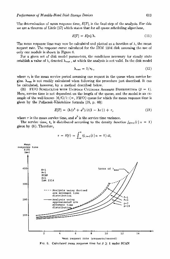
Performance of Movable-Head Disk Storage Devices 613
The determination of mean response time, E[T], is the final step of the analysis. For this we use a theorem of Little [17] which states that for all queue scheduling algorthms,
E[T] = E[n]/X. (11)
The mean response time may now be calculated and plotted as a function of ~, the mean request rate. The response curve calculated for the IBM 2314 disk assuming the use of only one module is shown in Figure 6.
For a given set of disk model parameters, the conditions necessary for steady state establish a value of k, denoted k . . . . . at which the analysis is not valid. In the disk model
Xmax = 1/T~, (12)
where r, is the mean service period assuming one request in the queue when service be- gins. km~ is not readily calculated when following the procedure just described. It can be calculated, however, by a method described below.
(B) F I F O SCHEDULING WITH UNIFORM CYLINDER ADDRESS DISTRIBUTION (~ : 1).
Here, service time is not dependent on the length of the queue, and the model is an ex- ample of the well-known M / G / l : (oo, FIFO) queue for which the mean response time is given by the Pollaczek-Khintchine formula [18, p. 40]:
E[T] = (X(r 2 + g2)/2(1 - Xr)) + r, (13)
where T is the mean service time, and a 2 is the service time variance. The service time, t, is distributed according to the density function ftJ,~=] (tl i~ = 1)
given by (6). Therefore,
0o
T = E[t) = tftln=l(t [ n = 1) dl,
Mean response time
E[T) (ms)
400
300
200
i00
s, s N=lM=l Locus of kmax ~/J/ SCAN IBM 2314
I ,'/ ~ ~ .... Analysis using derived ¢,'
arm movement time distribution
~ Analysis using ~" approximated arm movement time ~ ~ 8=7 distribution 8=19
FIG. 6.
i * i i i
4 6 8 i0 12
Mean request rate (requests/second)
Ca|eu]ated mean response time for ~ >_ I under SCAN
, DX 14

614 c . c . GOTLIEB AND G. H. MAcEWEN
which, on substitution, yields
r = [(aC)2(b + R ) 2 - (aC)~b 2 + (aC + b)~b "~ -- (aC + b + R)~(b + R ) ~ -- (aC + b) 4 + (aC + b + R ) ] / 2 R ( a C ) 2 + [2(aC 4- b) 4 - 2 (aC 4- b)b 3 4- 2 (aC 4- b 4- R ) (b 4- R ) 3 - 2 (aC 4- b 4- R)4] (14)
/ 3 R ( a C ) 2 4- [b 4 4- (aC 4- b 4- R ) 4 - (b 4- R ) 4 -- (aC 4- b)4]/4R(aC) 2.
Similarly,
E[t 2] = [(aC)e(b 4- R ) 3 - (aC)2b ~ 4- (aC 4- b)~b "J - (aC 4- b 4- R)2(b 4- R ) ~ - (aC 4- b) 5 4- (aC 4- b + R)5] /3R(aC) ~ 4- [2(aC 4- b) 5 - 2 (aC 4- b)b 4 4- 2 (aC 4- b 4- R ) ( b 4- R ) 4 (15) - 2 (aC 4- b 4- R ) 5 ] / 4 R ( a C ) 2 4- [55 4- (aC 4- b 4- R ) 5 - (b 4- R ) 5 -- (aC 4- b )5 ] /5R(aC) 2.
Calculating r and Ell 2] from (14) and (15) and a 2 from 2 = E[t~] _ r2, the mean response time can be calculated from (13). Figure 7 includes a response curve for the IBM 2314 disk assuming the use of only one module.
(C) S C A N SCHEDULING WITH NONUNIFORM CYLINDER ADDRESS DISTRIBUTION (~ > 1). Here, as with the uniform distribution model, we must find the distribution of the lengths of the n interior intervals created by n 4- 1 points on the interval (0, C) where the points are chosen as a random sample of size n 4- 1 from the distribution defined by fz (z). In the uniform case, it was sufficient to find the distribution of the ith interval, 1 < i < n, since all intervals were identically distributed. In the present case, the dis- tribution of a randomly chosen interval is required. The density function of this distribu- tion, which may be found directly [1] or through the use of order statistics [19], is
f; 1 g(8) = O~ + 1) A(u)A(u + 8) f~(z) dx + A(x) dx du. (16) U'~'8
Mean response time
E[T] (ms)
500
400
300
200
i00
M=i FIFO
Sai IBM 2314
Analysis using derived arm movement time ~ / distribution ~ ~ / A Z nalysisusing / approximated arm movement ~ /~/" time distribution /7 /
l i
4' 6' 8' 2 i0
Mean request rate (requests/second)
/
~=19
|
12
F*G. 7. Calculated mean response time for ~ >_ 1 under FIFO

Performance of Movable-Head Disk Storage Devices
f_tln(t{ n)
615
i/R
Approximated density function for $>1, n=2
--r----------[-~/] Density [ ~=i, n=- ' I~"- ~[functions _. _^ '1 ~ ' / f for $-i, n-z ; / I \ y / j B:i, n:l
b b+R b+R+aC
~-- E (B,n)
FIG. 8. Comparison of service time density functions
This function is intractable for any nontrivial fz (x))° Since fz (z) is taken here to be the beta distribution, f~ > 1, g(s) cannot therefore be used analytically to determine the arm movement distance. To overcome this difficulty, an approximation is made at this point in the analysis.
The approximation is based upon the assumption tha t the arm movement distance is a constant for every value of n, the number of requests in the queue. This constant, E ' (/~, n) , c is taken to be the mean arm movement distance. Thus E ' (~, n) = fo sg (s)ds.
The mean arm movement time is then E (~, n) = aE'(fl, n). Where needed (see formula (20)), E(/3, n) is calculated numerically u for given values of fl and n.
The approximated service time is
t = b + e T E ( ~ , n ) (17)
where b is the fixed portion of arm movement time, c is the channel service time, E(/~, n) is the variable portion of arm movement time, and t is distributed according to
t O, t < b --t- E ( ~ , n ) , ftla,,,(tlfl, n) = 1/R, b + E ( f ~ , n ) < t < b T R W E ( f l , n), (18)
[0, t > b -4- R -4- E(f~, n).
Figure 8 shows three of the density functions, from the family of functions derived for the t3 = 1 model, for n = 1, 2, and ~ . The approximated density function for fl > 1 and n = 2 is also shown in dot ted lines. The family of approximated density functions consists of identically shaped rectangular distributions displaced from the distribution for j3 = 1, n = ~ by an a m o u n t E ( f l , n) .
The true density functions, ftl~,~(tlfl, n), for fl > 1 are unknown. For a given value of n, however, the functions for ~ > 1 would be nonzero between b and b + R + aC and would have a lower mean value than the function for ~ = 1 since mean arm movement time would be less. As n increases, the true density functions and the approximate density functions both approach the rectangular distribution shown in Figure 8. The
,o Note that substituting fz(z) = l/C, 0 _< z _< C, yields g(s) = (n + 1)(1 -- s/C)'*, which agrees with (1), the formula previously used for the interval distribution when fz(z) was taken to be the uniform distribution. ** Calculation for the results shown used an 8-point Gaussian integration method.
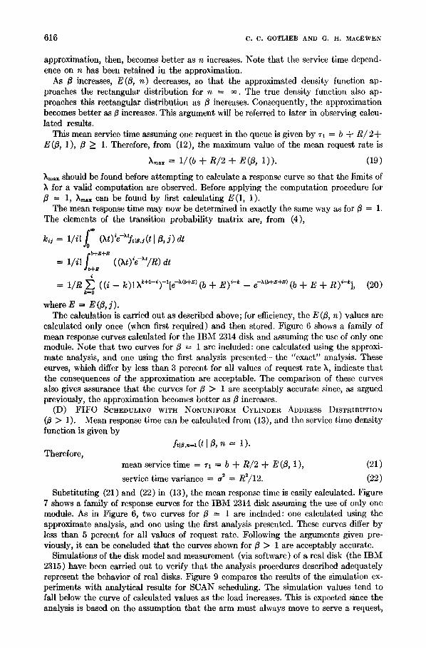
616 C.C . GOTLIEB AND G. H. MACEWEN
approximation, then, becomes better as n increases. Note that the service time depend- ence on n has been retained in the approximation.
As 8 increases, E(8, n) decreases, so that the approximated density function ap- proaches the rectangular distribution for n = ~ . The true density function also ap- proaches this rectangular distribution as 8 increases. Consequently, the approximation becomes better as ~ increases. This argument will be referred to later in observing calcu- lated results.
This mean service time assuming one request in the queue is given by rl = b -t- R~ 2 ÷ E ( 8 , 1 ), 8 _> 1. Therefore, from (12), the maximum value of the mean request rate is
hma. = 1/(b W R/2 + E(8, 1) ) . (19)
hma~ should be found before attempting to calculate a response curve so that the limits of for a valid computation are observed. Before applying the computation procedure for
8 = 1, hm~ can be found by first calculating E(1, 1). The mean response time may now be determined in exactly the same way as for 8 = 1.
The elements of the transition probability matrix are, from (4),
= (ht) e /t,0,¢(t[ 8,J) dt
f b÷E+R
= 1/i! ((ht)'e-~'/R) dt d b+E
i
= 1/R ~ ((i - k)! ~+l-')-'[e-~(b+E) (b + ~)'-~ -- e-~(b+E+~)(b + E + R)'-~], (20) k--0
where E = E (8, J). The calculation is carried out as described above; for efficiency, the E (8, n) values are
calculated only once (when first required) and then stored. Figure 6 shows a family of mean response curves calculated for the IBM 2314 disk and assuming the use of only one module. Note that two curves for 8 = 1 are included: one calculated using the approxi- mate analysis, and one using the first analysis presented--the "exact" analysis. These curves, which differ by less than 3 percent for all values of request rate h, indicate that the consequences of the approximation are acceptable. The comparison of these curves also gives assurance that the curves for 8 > 1 are acceptably accurate since, as argued previously, the approximation becomes better as 8 increases.
(D) FIFO SCHEDULING WITH NONUNIFORM CYLINDER ADDRESS DISTRIBUTION
(~ > 1). Mean response time can be calculated from (13), and the service time density function is given by
f t [B ,n -1 (t I S, n = 1). Therefore,
mean service time = 7"1 = b + R / 2 + E ( 8 , 1), (21)
service time variance = a 2 = R2/12. (22)
Substituting (21) and (22) in (13), the mean response time is easily calculated. Figure 7 shows a family of response curves for the IBM 2314 disk assuming the use of only one module. As in Figure 6, two curves for 8 = 1 are inclnded: one calculated using the approximate analysis, and one using the first analysis presented. These curves differ by less than 5 percent for all values of request rate. Following the arguments given pre- viously, it can be concluded that the curves shown for 8 > 1 are acceptably accurate.
Simulations of the disk model and measurement (via software) of a real disk (the IBM 2315) have been carried out to verify that the analysis procedures described adequately represent the behavior of real disks. Figure 9 compares the results of the simulation ex- periments with analytical results for SCAN scheduling. The simulation values tend to fall below the curve of calculated values as the load increases. This is expected since the analysis is based on the assumption that the arm must always move to serve a request,

Performance of Movable-Head Disk Storage Devices
Mean response time
E[T] (ms)
617
40(
300
200
i00
N=i M=i SCAN IBM 2314
8=1
Calculated ~ /
~ ~mulated (Runs 1 and 8)
FiG. 9.
I i I ! i !
2 4 6 8 i0 12 Mean request rate (requests/second)
Comparison of calculated and simulation results--SCAN
D
thus requiring at least the fixed portion of arm movement time. In practice, of course, the arm may not need to move, especially if ~ >> 1 or the load is heavy. The values de- rived from the simulations run at low request rates are sufficiently close to give assurance that the calculations do represent the behavior of the disk model.
Figure 10 compares the results of the measurement experiments with analytical results for SCAN scheduling. Again, the measured values tend to fall below the curve of cal- culated values as the load increases. Nevertheless, the measurements taken at low request rates are sufficiently close to give assurance that the calculations do represent the behavior of the model of the 2315 disk operating in a steady state condition.
4. The Multimodule System
Consider the M-module single-channel disk model represented by the set of queues in Figure 2 and the associated timing diagram in Figure 1. This model, de~ned in Section 2, is analyzed using a method based partially on a technique of Seaman et al. [5]; Seaman analyzes the channel queue by applying results from the "machine repair" queueing model. In this model there is a single repairman to service M machines, each of which may break down at any time. That is, the time to the next failure for each operating machine is exponentially distributed. A queue of inoperative machines awaiting repair may form.
In the disk model, the channel may be looked upon as the repairman in the machine repair model and the M model queues may each be looked upon as the machines. The event of a request leaving a module queue to joint the channel queue corresponds to the event of a machine breaking down and joining the queue for the repairman.
Seaman's channel queue analysis assumes an exponentially distributed channel ser- vice time; this analysis is generalized to permit a uniformly distributed channel service time. The analysis of Section 2 is then applied to calculate the mean response time for FIFO and SCAN scheduling.
Recall that the module queue server remains busy until the channel service time is

618 c . c . GOTLIEB AND G. H. MAcEWEN
Mean response time
E[T] (ms)
600
500
400
300
200
I00
®
.1 B-i- / 8=6
I I i ! : =
2 4 6 8 10
Mean request rate (requests/second)
FIG. 10. M e a s u r e d m e a n response t i m e - - S C A N
completed. Because of this interaction any one module queue, along with the channel queue, can be viewed as a single equivalent queue having a service t ime composed of: m, the arm movement t ime; q, the channel queueing time; and c, channel service time. Requests arrive at the equivalent queue with a mean request rate of k /M. If the mean and the variance of q can be determined, the mean response time for FIFO module queue scheduling can be calculated directly from
E[T] = (X/M(T 2 + a2)/2(1 -- hT/M)) + T,
where
and
T = mean service time = E[m] + E[q] + E[c],
(23)
(24)
a ~ = variance of service t ime = am 2 + aq 2 + ac 2. (25)
In order to find E[q] and aq 2, the channel queue is analyzed as follows. From the viewpoint of the channel queue, the M module queues can be looked upon as M sources, each of which generates requests a t an effective mean rate w. Assume tha t the requests are generated randomly in time, tha t is, requests arrive at the channel queue with exponen- t ially distr ibuted interarrival times. The M sources, because of the module-channel queue interaction described previously, do not, however, generate requests continuously; each source may contribute only one request a t a t ime to the channel queue and therefore does not generate requests if this contribution is in the queue. Note tha t
(a) the channel queue contains a t most M requests;

Performance of Movable-Head Disk Storage Devices 619
(b) w > h / M , since the mean arrival rate to the channel queue is h and the sources do not generate requests continuously.
The channel queue, as described here, is an example of the "machine repair" queueing model [18, p. 232]. Applying the theory which has been developed for such a queue [20] along with some general probabil i ty theory (see [1]), w is calculated as a function of using an i terative technique, 12 and E[q] and a~ are found to be
E[q] = ( M - 1 ) . R / 2 - ( 1 - ~rM-1)/W (26) where
lr~-1 = Prob [there are no requests in the channel queue immediately preceding completion of a service time],
M--1 2 a~ = ~ pk[R2/6 -- R2(1 -- pM)/9 + R2(M -- k -- 1)/12] (27)
k--0 where
pk = Prob [there are M - k requests in the channel queue a t any random time], O _ < k < i .
Tables of ~'M-1 and Pk, as functions of ~, can be calculated as described in [1]. We now examine the four possible combinations of scheduling (FIFO and SCAN)
with values of f~ = 1 and ~ > 1. (A) SCAN, f~ = 1. Channel queueing time, q, is assumed to be a constant; this ap-
proximation is necessary so tha t q can be incorporated into the previous analysis. This can be done by assuming tha t queueing time is par t of the fixed portion, b, of arm move- ment time. The equivalent queue is therefore identical to the single-module queue analyzed previously, and E (T) may be calculated by applying the corresponding single- module procedure with (i) b replaced by b -b E[q], and (ii) k replaced by h /M.
(B) FIFO, ~ = 1. Mean response time, E[T], is calculated directly from (23) where
t Tt r = r --~ E[q], = E[m] + E[c]
which is obtained from (14), 2' 2 t2 if2 q2t . jr 0-q2 0- 0-m 2 -~- ac E[t 2]
and E[f] is obtained from (15). (C) SCAN, /3 > 1. Following the argument of (a) above, E[T] is now calculated,
for SCAN and/~ > 1, by applying the corresponding single-module procedure with (i) b replaced by b -t- E[q], and (ii) h replaced by X/M.
(D) FIFO, B > 1. Mean response time is calculated directly from (23) where
T t ! ~" -- + E[q], ~- = E[m] + E[c] = b T R /2 T E(~, 1) (see (21)),
02 ---- ff2t ..~ 0-q2, O2~' = 0-m 2 "JC 0-c 2 "~ R2/12 (see (22)).
The values of parameters over which the calculations were performed are: M = 1, 2, 3, 4 (see footnote 12); R = 30, 40, 50 (maximum block transfer t ime of 5, 15, 25 ms) ; /~ = 1, 6 ; Scheduling: F IFO, SCAN.
12 Newton's method for solving the equation f(w) = O. Since f(w), as it occurs here, becomes a very long formula for m > 2, a formula manipulation system, FORMAC, was used to generate the formu- las for f(w). FORMAC is unable to evaluate formulas containing exponentials; consequently, the formulas were printed out, punched, and inserted into the Newton method program. This proce- dure became unmanageable for M > 4. For present purposes, however, calculations up to m = 4 are sufficient and no other method of generating the formulas was pursued.

620 c . c . GOTLIEB AND G. H. MAcEWEN
5. Use o.f Results
The improvement in mean response time resulting from SCAN, rather than FIFO, schedul- ing is illustrated in Figure 11. Note that the improvement is much greater for high re- quest rates. The improvement itself is not as significant as the smaller slope retained by the SCAN curve through higher request rates; this enables SCAN to operate satisfac- torily at values of ~ that would cause very long queues to build up under FIFO schedul- ing. SCAN, then, is most useful under very heavy loading conditions.
One can observe certain basic quantities illustrated in Figure 11 by hME(M, S), hsE(M, S), and ~lim(M, S):
hME(M, S)-- the change in E[T] produced by adding one module (thereby increasing the total amount of stored data by the capacity of a module) to an M -- 1 module con- figuration, assuming that h/M and the scheduling algorithm, denoted by S, are fixed. As shown, huE(M, S) for M = 2, hIM = 7.5, and S = FIFO, equals +18 ms.
~klira(M, S)-- the highest value of ~ for which E[T] falls below some given maximum allowable mean response time E[T] ..... As shown, ~lim(M, S) for M = 1, E[T]max = 240 ms, and S = FIFO, equals 7.5 requests/second.
hsE(M, S)-- the improvement in E[T] obtainable through scheduling (as opposed to no seheduling, i.e. FIFO), assuming that all other parameters are fixed. As shown, hsE(M, S) for M = 1, S = SCAN, and X = 7.5, equals --60 ms.
As a first approximation in estimating the changes resulting from adding more modules, one expects that adding m modules would, for example, increase the permissible range of
by some multiple of m. In other words, the quantity Mim (M, S) /M should not vary greatly as M increases. We find from Figure 9 the following variation:
M ~llm(M, S) ~llm(M, S)/M
1 7.5 7.5 2 14.5 7.3 3 20.4 6.8 4 25.2 6.3
klim (M, S) /M decreases as M increases. This decrease is to be expected from increasing congestion in the channel as the data transfer load increases; increasing M, and thereby ~, raises channel utilization which, as queueing theory predicts, results in a longer channel queue.
Channel congestion affects other quantities as well: hiE(M, S) indicates the cost in mean response time of connecting one additional module to a single channel. Assuming that each module has a mean request rate of 7.5 requests/second, hME(M, S) for S = FIFO varies as follows:
M AME(M, S) (ms) ~ME(M, S) (%)
2 18 8 3 57 22 4 160 51
Thus the addition of one module to a three-module system increases the mean response time of each of the three modules by 51 percent.
Fucther discussion, with examples, of the use of the results is given in [1]. In particular, different curves are plotted that illustrate the effect on E[T] of the module arm movement characteristics, thegrouping of files on adjacent cylinders, and the mean block length.
6. Extensions
Tables such as those represented by the data plotted in Figure 11 may be useful for evaluating system configurations without resorting to time-consuming and expensive simulation or measurement. To make comparisons between devices and to consider the

Performance of Movable-Head Disk Storage Devices
Mean response time
E[T] (ms)
FIFO
N = i '°°t M'1.2,3,4 I / / / / SCAN, Fzro / l / / / / B=i ! M-i / M=2 /M=3 / M:4 / IB-' ms 2
IBM 2314
300 SCAN
E [T]max ......... ¥ . . . . . 7- "
2ooi IV ME(M's/ V / ///
; 1; is 2; 2~ 3; Xlim(M, S)
Mean request rate (requests/second)
621
3~ " ~
FIG. 11. Variation in ELT] with M
trade-offs involved, similar tables are also needed for other devices such as drums and fixed head disks.
The system designer must, of course, be fully aware of the assumptions and approxi- mations upon which the calculation of the tables is based. These assumptions may not, however, seriously restrict the utility of the tables; in many design situations, the es- timates of system loading either are approximate or are bounds on an allowable range of load. Under such conditions tables provide: (a) a frame of reference within which the designer may work to evaluate various combinations of parameters; (b) some indica- tion of the theoretical limits within which the system must operate (given that the assumptions of randomness apply).
An empirical study of disk performance over a wide range of operating conditions is needed. Data from such a study would provide information about the applicability of the idealized disk model and, more importantly, would provide some insight into the behavior of real systems so that the model may be appropriately refined.
Although the SCAN scheduling algorithm was chosen for attention on the basis of system equity, the SSTF algorithm is not completely rejected; an analytical procedure for accurately determining the performance of disks using SSTF scheduling would contribute to understanding this algorithm. A modified SSTF may prove to be effective. For ex- ample, recording the waiting time of each data transfer request and giving service priority to requests that have waited an excessive amount of time, may prove to be effective under certain conditions. Unless the time limit were dynamically adjusted, however, this modified SSTF would degenerate to FIFO under a very heavy load.
.Both SCAN and SSTF are clearly better than FIFO with respect to mean response time. To investigate the characteristics of these as well as other algorithms [8] within a real system, experiments should be carried out by inserting a queue scheduling program

622
i
Module queueing
time
u L
C. C. GOTLIEB AND G. H. MAcEWEN
Module queue I. Channel queue ,I service time service time
Arm Rotational Channel Rotational Block motion delay to queueing delay transfer time sector time within sector . time
Module busy
Channel busy
Response time
FIG. 12. Timing diagram for IBM 3330 disk
module into the Input/Output Supervisor and measuring the performance under each algorithm. I t is encouraging to note in this regard that a version of SCAN scheduling has very recently been offered as an option in OS/360 [21]. 13
A hardware approach to reducing response time is taken in a recently marketed mow~ble-head disk, the IBM 3330. This device, available with 2, 4, 6, or 8 modules (as modules are defined here) eliminates use of the channel during part of the rotational
delay time. Channel utilization for a given value of X is thereby decreased and channel congestion is reduced accordingly.
The timing diagram for a 3330 disk model is shown in Figure 12. As in Figure 1, over- head times are ignored. The queueing diagram for the 3330 is the same as for the 2314 (Figure 2).
As with the 2314 model, the module queue server remains busy when a request leaves the module queue to join the channel queue (Time 1 ), until that request leaves the chan- nel queue (Time 2). Channel queueing time is either zero or a multiple of a full rotation time. Note that for a single-module configuration of such a disk, channel queueing time is always zero and the timing diagram reduces to that of Figure 4 (except for the chan- nel busy period shown in Figure 4). The model and analysis procedure described in Sections 2 and 3 are therefore valid for a disk of this type.
A multimodule disk model of a 3330-like disk can be analyzed as in Section 4 except that a new channel queue analysis, analogous to that contained in [1], is needed. The channel queue is similar to the drum model analyzed by Abate and Dubner [22] except for two important differences: first, the queue can only contain up to M requests; second, there are M, not one, distinct rotating surfaces. Nevertheless, Abate and Dubner's analysis may provide insight into the channel queue analysis needed here.
Note that it is important, in view of the flexible configuration of the 3330 disk (2, 4, 6, or 8 modules), to be able to analyze and compare multimodule models with differing numbers of modules.
The introduction of the IBM 3330 strengthens the opinion that movable-head disks will be important for a significant time to come. Recently, other types Of secondary storage devices, e.g. magnetic card devices, have become less important because they have not competed favorably with movable-head disks. At the same time, newer tech- nologies such as optimal recording have not progressed to a state whereby useful large capacity devices can be built.
za No information concerning performance measurements or implementation problems is currently available.

Performance of Movable-Head D i s k Storage Devices 623
ACKNOWLEDGMENTS. T h e a u t h o r s wish to t h a n k Professors J. J . H o m i n g a n d J. G. C. T e m p l e t o n for m a n y useful c o m m e n t s a n d suggest ions. T h e a u t h o r s also wish to t h a n k t h e N a t i o n a l Resea rch Counci l of C a n a d a for f inancia l ass is tance, a n d to acknowledge t h e p r o g r a m m i n g help of Miss M i n a Craig.
REFERENCES
1. MAcEwEN, G. H.
2.
3.
4.
5.
6.
7.
8.
9.
10.
11.
12.
13.
14.
15.
16. 17.
18. 19.
20. 21. 22.
23.
Performance of disk storage devices in computer systems. Ph.D. Th., Dep. of Computer Science, U. of Toronto, Toronto, Canada, 1971. FREEMAN, D . i . A storage hierarchy system for batch processing. Proc. AFIPS 1968 SJCC, Vol. 32, AFIPS Press, Montvale, N. J., pp. 229-243. GAVER, D. P. JR. Probabili ty models for multi-programming computer systems. J. ACM I.~, 13 (July 1967), 423-438. FIFE, D. W., AND SM:TH, J .L . Transmission capacity of disk storage systems with concurrent arm positioning. I E E E Trans. EC-1~4 (Aug. 1965), 575-582. SEAMAN, P. H., LIND, R. A., AND WILSON, T. L. An analysis of auxiliary storage activity. IBM Syst. J . 5, 3 (1966), 158-170. DENNING, P. J. Effects of scheduling on file memory operations. Proc. AFIPS 1967 SJCC, Vol. 30, AFIPS Press, Montvale, N. J., pp. 9-21. ABATE, J., DUBNER, H., AND WEINBURG, S.B. Queueing analysis of the IBM 2314 disk storage facility. J. ACM 15, 4 (Oct. 1968). 577-589. TEOREY T. J., AND PINKERTON, T. B. A comparative analysis of disk scheduling policies. Comm. ACM 15, 3 (Mar. 1972), 177-184. FRANK, H. Analysis and optimization of disk storage devices for time-sharing systems. J. ACM 16, 4 (Oct. 1969), 602--620. IBM System/360 component description--2314 direct access storage facility. Form A26-3599, IBM Syst. Ref. Library. FUCHS, E., AND JACKSON, P .E . Estimates of distributions of random variables for certain com- puter communications traffic models. Comm. ACM 13, 12 (Dec. 1970), 752-757. FELLER, W. An Introduction to Probability Theory and Its Applications, Vol. II . Wiley, New York, 1966. HARRIS, C .M. Queues with state dependent stochastic service rates. Oper. Res. 15, 1 (Jan. 1967), 117-130. HARRIS, C .M. Queues with state-dependent stochastic service rates. Ph.D. Th., Polytechnic Inst. of Brooklyn, Brooklyn, N. Y., 1966. KENDALL, D.G. Stochastic processes occurring in the theory of queues and their analysis by means of the imbedded Markov chain. Ann. Math. Slat. 25 (1953), 338-354. PARZEN, E. Stochastic Processes. Holden-Day, San Francisco, 1962. LITTLE, J. D .C . A proof of the queueing formula: L = XW. Oper. Res. 9, 3 (Mar. 1961), 383- 387. SAATY, T .L . Elements of Queuei~,g Theory with Applications. McGraw-Hill, New York, 1961. FOSTER, F . G . On stochastic matrices associated with certain queueing processes. Ann. Math. Slat. 24 (1953), 355-360. TAKACS, L. Introduction to the Theory of Queues. Oxford U. Press, New York, 1962. IBM Installation Newsletter, Issue No. 70&7, Apr. 1970. ABATE, J., AND DUBNER H. Optimizing the performance of a drum-like storage. IEEE Trans. C-18, 11 (Nov. 1969), 992-997. COFFMAN, E. G., KLIMKO, L. A., AND RYAN, BARBARA. Analysis of scanning policies for re- ducing disk seek times. S I A M J. Comp. (to appear).
RECEIVED MARCH 1971; REVISED MAY 1972
Journal of the Association for Computing Machinery, Vol. 20, No. 4, October 1073