performance networks - ahmadu bello university queueing system”, (b) ... queueing theory to...

PERFORMANCEANALYSIS OF

TELECOMMUNICATIONSAND

LOCAL AREANETWORKS

THE KLUWER INTERNATIONAL SERIESIN ENGINEERING AND COMPUTER SCIENCE

PERFORMANCEANALYSIS OF

TELECOMMUNICATIONSAND

LOCAL AREANETWORKS

by

Wah Chun ChanThe University of Calgary

KLUWER ACADEMIC PUBLISHERS NEW YORK, BOSTON, DORDRECHT, LONDON, MOSCOW

eBook ISBN: 0-306-47312-7Print ISBN: 0-792-37701-X

©2002 Kluwer Academic PublishersNew York, Boston, Dordrecht, London, Moscow

All rights reserved

No part of this eBook may be reproduced or transmitted in any form or by any means, electronic,mechanical, recording, or otherwise, without written consent from the Publisher

Created in the United States of America

Visit Kluwer Online at: http://www.kluweronline.comand Kluwer's eBookstore at: http://www.ebooks.kluweronline.com

To my wife Yu-Chih and our children

Eileen, Jean, Vivian and An-Wen

Wah-Chun Chan

This page intentionally left blank.

ABOUT THE AUTHOR

Wah-Chun Chan is Professor of Electrical and ComputerEngineering at the University of Calgary at Calgary, Alberta, Canada.He received his B.Sc. degree from National Taiwan University, M.Sc.degree from the University of New Brunswick and Ph.D. degree fromthe University of British Columbia. Prior to his appointment at theUniversity of Calgary in 1967, he was a Systems Engineer forNorthern Electric Co. (now Nortel Technology) in Ottawa, Ontario.

Dr. Chan has published extensively in professional journals. Inaddition to telecommunication systems, his research interests includeoptimal control systems, variable structure control systems, queueingtheory and reliability analysis.

Dr. Chan and his co-workers were awarded the IEE AmbroseFleming Premium in 1974 for the papers: (a) “Waiting time incommon-control queueing system”, (b) “Transient in a single-serverqueueing system”, and (c) “Multiserver computer controlled queueingsystem with preemptive priorities and feedback”.

PREFACE

A telecommunication network conveys information by means oftransmission links. These links are connected by switching systems andcontrolled by a signaling system. The network provides many services forexchange of information over distance. Thus, public-switched telephonenetworks as well as computer networks have become an integral part ofmodern society's infrastructure. Today, these networks are used extensivelyin business, in social life, in education and in entertainment. In particular,virtually all engineers and computer scientists need to understand the basicprinciples governing the operation and performance of telecommunicationsand computer networks.

SCOPE

The book is concerned with performance analysis intelecommunications and local area networks. It is designed to provide anunderstanding of the fundamental principles of teletraffic engineering.Emphasis is placed on the modeling techniques using queueing theory for thepublic-switched telephone network and local area networks.

The Telephone Network. The telephone network interconnectsmillions of telephones around the world. It offers a two-way, circuit-switched voice service and achieves a quality of service by setting up acommunication path between two or more users.

Local Area Networks. A local area network (LAN) providesinterconnection of a variety of data communicating devices within a smallarea. It is generally privately owned by a single organization. A typicalexample of the LAN technology is the Ethernet.

WHY WRITE SUCH A BOOK

These exist several books on the performance analysis of datanetworks or computer networks. Most of them are at a higher mathematicallevel.

This book attempts to present the essentials of queueing theory at alevel that undergraduate students and practicing engineers can understand.After presenting the theory, applications to the analysis of practical networksfollow.

WHO ARE THE INTENDED READERS

The book should appeal to undergraduate students. It can be used as atextbook for a course on telecommunications and local area networks. Withsome supplementary material the book can also be used for a graduatecourse. The practicing engineers may find the book useful for self-study,because of the emphasis on practical applications.

The material covered in this book is based on a series of lecture notesdeveloped by the author in the Department of Electrical and ComputerEngineering at the University of Calgary, Alberta, Canada.

The text is organized as follows. After an introductory chapterpresenting some basic concepts and terminology of teletraffic engineering,Chapter two provides some basic theory on transmission systems. Chapterthree discusses the congestion problem in switching systems, while Chapterfour introduces the basic principles of queueing theory. Emphasis is placedon modelling techniques and the physical significance of the theory. The restof the text, Chapter five to Chapter ten, is devoted to applications ofqueueing theory to performance analysis of the public-switched telephonenetworks and local area networks. There are numerous examples whichillustrate the applications of the theory. The text assumes that the reader hassome background in elementary probability theory and random processes.

ACKNOWLEDGEMENTS

The author owes a special thanks to Mrs. Ella Gee for her skillfultyping of the manuscript several times. In addition, the author wishes tothank his wife, Jane (Yu-Chih Liu). Without her support and understandingthis text could not have been written.

Contents

Preface . . . . . . . . . . . . . . . . . . . . . . . . . . . . . . . . . . . . . . . . . . . . . . . . . . . . . . . . . . . . . . . . . . . . . . . . . . . . . . . . . . . . . . . . . . . . . .

1. INTRODUCTION TO TELECOMMUNICATION SYS-TEMS . . . . . . . . . . . . . . . . . . . . . . . . . . . . . . . . . . . . . . . . . . . . . . . . . . . . . . . . . . . . . . . . . . . . . . . . . . . . . . . . . . . . . .

1-1 Introduction . . . . . . . . . . . . . . . . . . . . . . . . . . . . . . . . . . . . . . . . . . . . . . . . . . . . . . . . . . . . . . . . . . . .1-2 Examples of Telecommunication Systems .......................1-3 Elements of a Telecommunication System .......................1-4 Topological Structure of Telecommunication

Networks .........................................................................1-5 Signals and Their Characteristics .....................................1-6 Transmission Media and Their Characteristics .................1-7 Quality of Service in Telephone Networks ......................1-8 Fundamentals of Voice Traffic and Data Traffic ..............1-9 Outline of the Book ..........................................................1-10 Summary .........................................................................

References ........................................................................Problems ...........................................................................

2. TRANSMISSION SYSTEMS . . . . . . . . . . . . . . . . . . . . . . . . . . . . . . . . . . . . . . . . . . . . . . . . . . .2-1 Introduction ......................................................................2-2 Subscriber Loop Design ...................................................

2-2-1 Basic Resistance Design ......................................2-2-2 Basic Transmission Design ..................................

2-3 Unigauge Design for Telephone Customer LoopPlants ...............................................................................

2-4 Signal Multiplexing ..........................................................2-4-1 Space-Division Multiplexing ................................2-4-2 Frequency-Division Multiplexing .........................2-4-3 Time-Division Multiplexing .................................

ix

115

13

152121222428313232

3333404144

5152525354

xii

2-5 Digital Transmission Systems ..........................................2-5-1 Asynchronous Transmission ................................2-5-2 Synchronous Transmission ...................................

2-6 Optical Fiber Transmission Systems ................................2-7 Summary ..........................................................................


3. SWITCHING SYSTEMS..........................................................3-1 Introduction ......................................................................3-2 Centralized Switching .......................................................3-3 Switching Techniques .......................................................

3-3-1 Space-Division Switching ....................................3-3-2 Time-Division Switching .....................................3-3-3 Frequency-Division Switching .............................

3-4 Congestion in Space-Division Switching Networks .........3-4-1 Switching Matrices ...............................................3-4-2 Multistage Networks ............................................3-4-3 Link Systems ........................................................

3-4-3-1 Two-Stage Link Systems ........................3-4-3-2 Three-Stage Link Systems ......................3-4-3-3 Three-Stage Link Systems Using a

Collection Stage .....................................3-5 Nonblocking Networks .....................................................3-6 Three-Stage Networks with Retrials .................................3-7 Congestion in Time-Division Switching Networks ..........3-8 Summary ...........................................................................

References ..........................................................................Problems .............................................................................

4. MODELING OF TRAFFIC FLOWS, SERVICE TIMESAND SINGLE-SERVER QUEUES . . . . . . . . . . . . . . . . . . . . . . . . . . . . . . . . . . . . . . .

4-1 Introduction ......................................................................4-2 The Poisson Input Process ...............................................

55606062656666

69697276767778798284878890

9296

100101112112113

117117121

4-2-1 Distribution for Number of Arrivals in a FixedTime Interval .......................................................

4-2-1-1 Superposition of Independent PoissonInput Traffic Flows ................................

4-2-1-2 Decomposition of a Poisson Flow ..........4-2-2 The Interarrival Time Distribution .......................

4-2-2-1 The Markov Property or MemorylessProperty ..................................................

4-2-2-2 Relationship between the PoissonArrival Process and the InterarrivalTimes ......................................................

4-3 The Service Time Distribution .........................................4-4 The Residual Service Time Distribution ..........................4-5 The Birth and Death Process ............................................4-6 Little’s Formula for Mean Values for a General

Queue ..............................................................................4-7 The M/M/l Queue ............................................................4-8 The Pollaczek-Khinchin Formulas for the M/G/1

Queue ..............................................................................4-9 The GI/M/1 Queue ...........................................................4-10 The M/G/1 Queue with Priority Discipline .....................4-11 The M/G/1 Queue with Vacations ...................................4-12 Summary ..........................................................................

Appendix A - Review of Probability Theory ...................Appendix B - Review of Markov Chain Theory .............References ........................................................................Problems ...........................................................................

5. THE ERLANG LOSS AND DELAY SYSTEMS . . . . . . . . . . . . . . . . . . .5-1 Introduction ......................................................................5-2 The Erlang Loss System ..................................................5-3 The Erlang Delay System .................................................5-4 The Combined Delay and Loss System ...........................5-5 The Outside Observer’s Distribution and the

Arriving Customer’s Distribution .....................................

xiii

122

127130133

136

136138140143

154158

168186191198198200206211212

224224225237245

247

xiv

5-6 The Waiting Time Distribution Function for the ErlangDelay System with Service in Order of Arrival ...............

5-7 The Waiting Time Distribution Function for theCombined Delay and Loss System with Service inOrder of Arrival ................................................................

5-8 Overflow Traffic ...............................................................

5-9 The Equivalent Random Method .......................................5-10 Summary .........................................................................

References .......................................................................Problems .........................................................................

6. THE ENGSET LOSS AND DELAY SYSTEMS . . . . . . . . . . . . . . . . . . . .6-1 Introduction ......................................................................6-2 The Engset Loss System ..................................................

6-3 The Arriving Customer’s Distribution for the EngsetLoss System ......................................................................

6-4 The Offered Load and Carried Load in the EngsetLoss System ......................................................................

6-5 The Engset Delay System ................................................6-6 The Waiting Time Distribution Function for the Engset

Delay System with Service in Order of Arrival ...............6-7 The Offered Load and Carried Load in the Engset

Delay System ....................................................................6-8 The Mean Waiting Time in the Engset Delay System

with Service in Order of Arrival ......................................6-9 Summary ..........................................................................


7. INTRODUCTION TO LOCAL AREA NETWORKS . . . . . . . . . . .7-1 Introduction ......................................................................7-2 Description of Local Area Networks ................................7-3 Channel Access Techniques .............................................7-4 Fixed Assignment Access Methods ..................................

7-4-1 Frequency-Division Multiple Access ......................

251

256258263276277277

284284284

287

289292

294

296

296300301301

304304305308309310

7-4-2 Time-Division Multiple Access ..............................7-4-3 Code-Division Multiple Access ..............................

7-5 Random Access Methods .................................................7-5-1 Pure ALOHA Networks ........................................7-5-2 Pure ALOHA Networks with Captures .................7-5-3 Slotted ALOHA Networks ....................................7-5-4 Slotted ALOHA Networks with Captures .............

7-6 Central Control Access Methods ......................................7-7 Summary ..........................................................................


8. POLLING NETWORKS ...........................................................8-1 Introduction ......................................................................8-2 Operation of Polling Networks .........................................8-3 Performance Analysis of Polling Networks .....................8-4 Summary ..........................................................................


9. TOKEN RING NETWORKS . . . . . . . . . . . . . . . . . . . . . . . . . . . . . . . . . . . . . . . . . . . . . . . . . . .9-1 Introduction ......................................................................9-2 Token Ring Networks ......................................................9-3 Operation of Token Ring Networks .................................9-4 Performance Analysis of Token Ring Networks ..............

9-4-1 Average Transfer Delay for Multiple-TokenOperation .................................................................

9-4-2 Average Transfer Delay for Single-TokenOperation .................................................................

9-4-3 Average Transfer Delay for Single-PacketOperation .................................................................

9-5 Operation of Slotted Ring Networks ................................9-6 Performance Analysis of Slotted Ring Networks .............9-7 Register Insertion Rings ...................................................

xv

311315318318324325331331333334335

339339341342353354354

358358359360365

367

368

370373375381

xvi

9-8 Operation of Register Insertion Ring Networks ...............

9-9 Performance Analysis of Register Insertion RingNetworks .........................................................................

9-10 Summary ...........................................................................References ........................................................................Problems ...........................................................................

10. RANDOM ACCESS NETWORKS . . . . . . . . . . . . . . . . . . . . . . . . . . . . . . . . . . . . . . . .10-1 Introduction ....................................................................10-2 Performance Analysis of Slotted ALOHA with

Poisson Input .................................................................10-3 Performance Analysis of Slotted ALOHA with a

Finite Number of Stations ..............................................10-3-1 Throughput Analysis ..........................................10-3-2 Average Transfer Delay .....................................

10-4 Performance Analysis of Slotted ALOHA byEquilibrium Point ...........................................................

10-5 Carrier-Sense Multiple Access (CSMA) Protocols ........10-5-1 Throughput Analysis of Non-Persistent

CSMA ................................................................10-5-2 Throughput Analysis of Slotted Non-

Persistent CSMA ................................................10-6 Carrier-Sense Multiple Access with Collision

Detection (CSMA/CD) Protocols ...................................10-7 Summary ........................................................................

References .....................................................................Problems ........................................................................

Appendix A - Determination of qn and qr .............................Appendix B - Determination of the Limiting Values of qn

and qr .......................................................................................

Answer to Selected Problems . . . . . . . . . . . . . . . . . . . . . . . . . . . . . . . . . . . . . . . . . . . . . . . . . . . . . . . . .

Index ....................................................................................................

381

384394394395

399399

400

405408409

414419

422

428

432443444445449

453

456

462

CHAPTER 1

INTRODUCTION TO TELECOMMUNICATION SYSTEMS

1-1. INTRODUCTION

Telecommunications has played a vital role in the advancement ofengineering and science. In addition to its importance in public switchedtelephone network (PSTN), radio and television networks, the Internet, andATM networks, telecommunications has become an important and integralpart of modern society. For example, telecommunications is essential inworldwide airline reservation systems. It is also essential in commercialdata processing industries, in remote accessing of data bases, ininformation and financial services, in inventory control systems, inautomatic teller systems, and in automated order systems.

Since advancement in the theory and practice of telecommunicationsprovide the means for attaining good quality of service in voice and datacommunications, sharing data bases and computer resources, etc., mostengineers and scientists should have a good understanding of thefundamental concepts of telecommunications.

Historical Overview. The first significant work intelecommunications was F.B. Morse’s code for telegraphy. Othersignificant works in the early stages of the development oftelecommunications were due to A.G. Bell, G. Marconi and C.E. Shannon,among many others. In 1876, Bell invented a telephone system. In 1897,Marconi patented a wireless telegraph system. Teletypewriter service wasinitiated in 1931. Satellite communication was proposed by J. Pierce in1953 and began service in 1962. During the decade of 1960, TV systemsand cable TV services were offered commercially. Starting in 1969, theARPA net created the world's first network for computer communications.The fundamental basis of the ARPA net is that messages are transmitted ina store-and-forward manner.

Store-and-forward packet switching was invented by P. Baran in 1961in the United States. He proposed that if messages are divided into smallerunits called packets for transmission, it would be more reliable, lesssusceptible to nuclear annihilation, and more economical than the PSTN.By the early 1980s, computer communication networks, such as the ARPA

2 CHAPTER 1

net, the Systems Network Architecture (SNA) of IBM, and the DEC net ofDigital Equipment Corporation, etc. were interconnected to form theInternet.

In 1968, A.G. Fraser proposed the concepts of virtual circuits andfixed-size packets for Spider, the first asynchronous time-divisionmultiplexing (ATDM) network. Fraser’s work laid the foundation forasynchronous transfer mode (ATM) networking. By the late 1980s,CCITT agreed in principle that the broad-band integrated services digitalnetwork (B-ISDN) would be built using ATDM, and the internationalstandard was named ATM (asynchronous transfer mode).

Unlike the PSTN and the Internet, ATM technology is still underdevelopment. ATM networks try to combine the ideas of the telephonenetwork, such as connection-oriented service and end-to-end quality ofservice, and those of the Internet, such as the virtual circuits, fixed-small-size packets and integrated services.

Definitions. In order to provide the service which permits people ormachines to communicate at a distance, a telecommunication system mustprovide the means and facilities for connecting the user terminals ortelephones at the beginning of the service and disconnecting them when theservice is completed.

In telephone systems, each subscriber telephone is connected by asubscriber line to a central switching point, called a switching center, themain function of which is to provide immediate connection between pairsof subscribers. The term telephone call, or simply call, means the demandto set up a connection. A call can be regarded as a series of dialingattempts to the same number, where the last attempt is either abandoned orresults in a successful connection. The subscriber line, also known as thesubscriber loop, is the pair of wires connecting the subscriber to the localswitching center. The subscriber loop provides a path for the two-wayspeech signals, ringing, switching and supervisory signals, and ispermanently associated with a particular subscriber. The end office is thelocal central switching center typically serving only subscriber lines. Toset up a connection, the end office must perform switching, signaling, andtransmitting functions.

In automatic switching centers, the connections are performed bymeans of switching elements, generally referred to as switches. Atelephone switch actually has two parts: the switching hardware carrying

CHAPTER 1 3

voice, and the switch controller handling call set-up and tear-down signals.

In studying telecommunication engineering, we need to defineadditional terms that are necessary to describe telecommunication systems:

Trunks. A trunk in telephone systems is a communication path thatcontains shared circuits that are used to interconnect central offices; ingeneral, 2-wire lines are used for interlocal centers and 4-wire lines forintertoll centers.

Trunk Groups. A trunk group is a group of trunks between twopoints, both of which are switching centers and/or individual messagedistribution points, and which employ the same multiplex terminalequipment.

Junctors. A junctor is a connection between networks in the samecentral office. Its function is equivalent to an interoffice trunk.

Links. A link is a transmission path used to make a connectionbetween successive stages of a switching network.

Network. A network is a set of communication links and switcheswhich, when activated, is capable of supporting a multiplicity of distincttransmission paths for voice or data transmissions.

Central Offices. A central office is a central switching center thatcomprises a switching network and its control and support equipment.

Toll Points. A toll point is a class 4 (switching) office not offeringoperator assistance for incoming calls.

Toll Centers. A toll center is a class 4 office offering operatorassistance for incoming calls.

Tandem Offices. A tandem office is a switching center betweenlocal offices, reducing the number of direct trunks required.

Blocking. Blocking is the state of a group of paths between twopoints in a network in which all the paths are occupied and hence nofurther interconnections are possible.

4 CHAPTER 1

Blocking Network. A blocking network is a network that, undercertain conditions, may be unable to set up a connection from one end ofthe network to the other. In general, all networks used intelecommunications are of the blocking type.

BORSCHT Circuit. A BORSCHT circuit is a line circuit in thecentral office. It is used as a mnemonic for the functions that must beperformed by the circuit: Battery, Overvoltage, Ringing, Supervision,Coding (in a digital office), Hybrid and Testing.

Modems. A modem (modulator/demodulator) is a device whichmodulates and demodulates signals transmitted over communicationfacilities. The modulator is for transmission and the demodulator is forreception. A modem is used to permit digital signals to be sent overanalog lines.

Multiplexing. Multiplexing is a means for the division of atransmission facility into a number of channels either by splitting thefrequency band of the channel into narrower bands, each of which is usedas a distinct channel (FDM, frequency-division-multiplexing), or byallotting the entire channel to a number of users, one at a time on a time-shared basis (TDM, time-division-multiplexing).

Packets. A packet is a group of binary digits including data andcontrol information arranged in a specified format which is transmitted as abasic unit.

Protocols. A protocol is a well-defined set of rules or conventionswhich governs the format and control of information that is transmittedthrough a network or that is stored in a data base. The information may bevoice, text, data or image.

Telecommunications. The term telecommunications is a service thatpermits people and machines to communicate at a distance. It includestelephony, video-telephony, data transmission, teleconferencing, e-mail, etc.

Stations. A station in a telecommunication system is the device usedas a means of communication by the user to the system and to other users.It includes telephone sets, terminals, printers, computers, or other types ofdata-communicating and data-handling devices.

CHAPTER 1 5

1-2. EXAMPLES OF TELECOMMUNICATION SYSTEMS

In this section, we shall present several examples oftelecommunication systems.

Step-by-Step (S × S) Systems. The basic principle of a step-by-stepsystem is illustrated in the schematic diagram in Figure 1-1. The S × Ssystem makes use of two-dimensional stepping switches. These steppingor selection switches are designed for both vertical and horizontalmovements, which are called the selection and hunting stages, respectively.They can step a maximum of ten levels vertically in unison with dialpulses and then, in the hunting stage, automatically rotate horizontally overten positions to search for an idle path to the next selector or other circuit.They are directly controlled by the dialed pulses.

The line finders are simpler switches, one for each group of incomingsubscriber lines. The line finder, once connected, supplies a dial tone tothe calling subscriber.

To illustrate the processing of an intraoffice call within the S × Ssystem, consider the four-digit line numbers 2345 to be called from asubscriber. When the calling subscriber initiates a call (handset off-hook),an idle line finder (always associated with a selector) finds and connects tothe calling line. A dial tone is sent to the calling party by this first

6 CHAPTER 1

selector. Dialing the first digit, 2, steps the first selector vertically to itssecond level. This first selector then rotates horizontally to select an idlepath to a second selector that serves the 2000 - 2999 number series. Thenext digit, 3, will step the second selector to its third level where it willhunt for an idle path to connectors associated with lines in the 2300 - 2399number sequence. The digit, 4, will cause the connector switch to move toits fourth level. Since the connector has no' hunting feature, the last digit,5, will move this connector horizontally 5 positions, thereby connecting tothe called line number 2 3 4 5 . The connector next tests the called line. Ifit is idle, ringing current is applied. If it is busy, a busy tone is returned tothe caller.

The S × S system has the advantage of being inexpensive for smallsystems and highly reliable due to the distributed nature of equipment.However, the system has several drawbacks:

1. Since the office code digits specify the exact levels to which selectorsare stepped, it is not feasible to select an alternate route for interofficecalls if all the trunks are busy.

2. The last two digits of the called line number are specificallydetermined by their locations on the connector. Congestion couldarise when the connectors are heavily loaded.

Crossbar Systems. The crossbar switch is the simplest space-division switch. The crossbar switching system employs crossbar switchesand common control in order to obtain full access and nonblockingcapabilities. Active elements called crosspoints are placed between inputand output lines. In common control switching systems, the switching andthe control operations are separated. This permits a particular group ofcommon control circuits to route connections through the switchingnetwork for many calls at the same time on a shared basis.

The principal control device of the crossbar system consists of twotypes of controllers known as originating markers and terminating markers(see Figure 1-2). Each marker is capable of advancing the state of a call,but only remains with a call for about one-half second. Each intraofficecall is served by one originating marker and one terminating marker duringits setup.

CHAPTER 1 7

The philosophy of design of the No. 1 Crossbar system is based onthe assumption that the majority of traffic handled will be interoffice. It isoften used for telephone service in large metropolitan areas.

The originating calls are served by originating senders (devices forreceiving and buffering dialed digits) and markers (controllers capable oftranslating dialed digits and locating idle paths and trunks for routingcalls). After the originating marker sets up the connection, the originatingsender sends the dialed digits to the terminating sender, which calls in aterminating marker to complete the connection.

After having performed their operations, the originating andterminating senders and markers drop off. The originating senderdisengages after transmitting the last four digits, and the terminating senderreleases after signaling the incoming trunk circuit to ring the called stationor to return a busy tone to the calling station.

For intermediate size central offices with low and primarily intraofficetraffic, the No. 5 Crossbar system shown in Figure 1-3 has been widelyused in North America. Compared to the No. 1 Crossbar system, themarkers of a No. 5 Crossbar system are given more control functions andthe sender functions are reduced and modified. Originating registers accept

8 CHAPTER 1

dialed digits and need only transmit information to a sender for anoutgoing call. Two types of markers are employed, one for dial tonecontrol and the other for completing call connections.

The processing of an interoffice local call is as follows. A subscriberlifting the handset to initiate a call will activate the line relay on aparticular line-link frame, which in turn activates the associated connectorto seize an idle dial-tone marker. The dial-tone marker locates the callingline, and secures an idle originating register (a storage element capable ofstoring a number) on a trunk-line frame. It then closes a selected pathfrom the calling line terminals, through the junctor group and the trunk-linkframes, and to the originating sender before releasing. The originatingsender sends a dial tone to the calling party, and then receives andtemporarily stores the dialed digits. As soon as all the seven digits havebeen received, the originating sender calls for an idle completing markerand transmits the called line number to it.

Upon receiving the digits of the called number, the completingmarker identifies the office code. If it is an interoffice call, then thecompleting marker seizes an idle outgoing sender and transmits to it allseven digits received from the originating register. At the same time, the

CHAPTER 1 9

completing marker selects an idle outgoing trunk circuit on the trunk-linkframe to the distant central office. If the call is an intraoffice one, thecompleting marker directs the outgoing sender to prepare to transmit onlythe last four digits corresponding to the called line number and then closesa path to connect the calling line through the trunk-link frame to the calledline on the line-link frame. Note that for an interoffice call, the incomingtrunk in the distant central office is the terminating end of the previouslyselected outgoing trunk in the calling office.

When an incoming trunk is seized by the outgoing trunk circuit in thecalling office, it selects an incoming register. This register then signals theoutgoing sender in the calling office to send the four digits of the calledline number. It also selects an idle completing marker and forwards thefour digits and other related data to the marker. The marker then selectsthe particular line-link frame and locates and tests the called line. If it isidle, the marker selects a path to connect the called line on the line-linkframe with the incoming trunk on the trunk-link frame, and then releases.If the called line is busy, the marker instructs the incoming trunk circuit tocause its associated outgoing trunk circuit in the calling office to send abusy signal to the calling party. The outgoing trunk circuit supervises thecall and also controls the disconnection of the operated crosspoints of thecrossbar switches on the line-link and trunk-link frames when the callingparty hangs up the phone.

Stored-Program Control Electronic Switching System. Thestored-program control (SPC) electronic switching system (ESS) offersmuch greater flexibility, maintainability, lower cost and larger capacity thancrossbar switching systems. The former two advantages are the result ofthe stored-program control approach used, and the latter two are due tosolid-state electronic technology.

The major impact of electronic switching has been in the speeds ofswitching and control. Both the S × S and crossbar switching systems areelectromechanical systems. Their switching and control functions mayrequire several milli-seconds. With electronic switching, they require onlya few nano-seconds. The high switching speed makes it possible to designa single common control for the entire system.

Other advantages of electronic switching systems include the longservice life of the equipment and its capacity for adapting new features andservices without changing the system design. This design flexibility is the

10 CHAPTER 1

result of utilizing the stored program and changeable memory concepts forprocessing calls in electronic switching systems.

Figure 1-4 shows the schematic diagram for the organization of aspace-division ESS. The principal elements of the system are grouped intotwo main parts: the central processor and the switching network. Thesetwo parts are functioning separately. The central processor consists of aset of program stores (semipermanent memory), a set of call stores(temporary memory), and a central control. The principal peripheralequipment associated with the central processor are the subscriber lines andline scanners, junctors and junctor scanners, trunks and trunk scanners,signal distributors, and the master control center.

CHAPTER 1 11

There is a continuous exchange of information between the centralcontrol and the call store as well as the program store. This informationmay concern the state of subscriber lines, paths in the switching networkand outgoing trunks. Instructions for the call-processing operation arestored in the (semipermanent memory) program store. Informationconcerning the progress of a call is stored in the (temporary memory) callstore.

The switching network, comprised of the line-link frame, junctorgroups, and trunk-link frame, interconnects calling subscribers' lines withselected outgoing or intraoffice trunk circuits.

The line scanners, junctor scanners and trunk scanners are used toconstantly monitor subscriber lines, junctors, and trunk circuits for changesin their status. For example, a subscriber line may change its status fromon-hook to off-hook, indicating that a call (request for service) has beeninitiated. On the other hand, a subscriber line may change its status fromoff-hook to on-hook, indicating that a call has been terminated ordisconnected. A junctor circuit or trunk circuit may be idle or busy.Information concerning the status of lines, junctor circuits and trunkcircuits is detected by the corresponding scanners and periodically sentback to the central control.

The master control center administers the operation and maintenanceof the entire central office. It provides information for accounting, systemoperations and trouble reports.

The ARPA Net. The ARPA (Advanced Research Project Agency)net was developed to interconnect the various types of large computersthroughout the United States, allowing users at one computer center toaccess facilities at other computer centers at a distance. It is a resource-sharing communication network in which messages are first segmented intosmaller fixed-size units called packets. The packets traverse the networkindependently in a stored-and-forward manner until they reach thedestination node, where they are reassembled into the original message.Thus many packets of the same message may be transmittedsimultaneously in the network using different paths, thereby providing thepipelining effect in reducing the message transfer delay.

The primary functions of the ARPA net comprise message storage,coding, routing, flow control and error control, among others. These

12 CHAPTER 1

functions are performed by communication processors known as IMPs(Interface Message Processors).

When a complete message is received at the destination IMP, anacknowledgement will be sent back to the sender node, indicating thecorrect delivery of the message.

Message routing in the ARPA net uses the locally determined routingtechnique. Each node in the ARPA net makes its own decision as towhich node a given packet will be forwarded next.

The design objective for the ARPA net is to minimize the costsubject to the constraint that the average message delay between any twonodes be 0.2 second.

The SITA Network. The SITA (Societe Internationale deTelecommunications Aeronautiques) network is a worldwide airlinereservations network. It also handles airline teletype messages usingcircuit-switching techniques.

There are two types of traffic handled by the SITA network: theinquiry/response traffic labeled as type A and the telegraphic traffic labeledas type B.

The type A traffic consists of inquiries and responses between theagents, terminals in airline offices, and their associated reservationcomputers located at some geographic distance. The type B traffic includestelegraphic messages destined to and generated by airline teleprinters andcomputers, and messages to and from local Telex networks. In general,type A messages are much shorter than type B messages. Furthermore,type A messages receive priority over type B messages when traversing thenetwork. For the type A messages, the average response time is 3 seconds,while that for type B messages is in the order of several minutes.

Agents’ terminals are polled cyclically by the processor asking themto transmit (if any) waiting inquiry messages. Upon receipt of a pollingmessage, the agent will transmit his waiting inquiries to the processor.

Ethernet. The Ethernet is a baseband mode, broadcast bus-type localarea network designed at the Xerox Palo Alto Research Center, whosetransmission medium is a coaxial cable named the Ether. The accessmethod used is the carrier-sense multiple access with collision detection

CHAPTER 1 13

(CSMA/CD).

Since there is no centralized control structure superimposed onto theEther, it is purely a passive communication medium. Control of thenetwork is therefore distributed throughout the system.

The Ethernet specifications and the IEEE 802 standards specify thebaseband buses, the use of 50 coaxial cable and terminators, and a datarate of 10 Mbps. The terminators absorb signals, preventing reflectionfrom the ends of the bus. The main components of an Ethernet are: acoaxial cable with terminators, taps, transceivers, interfaces, andcontrollers. The transceiver makes a physical connection to the Ether by atap. The interface is used to serialize and deserialize the bit streamsbetween the controller and the transceiver. The controller is responsiblefor the correct transmission and reception of packets across the network.Figure 1-5 shows the main components of an Ethernet connection.

1-3. ELEMENTS OF A TELECOMMUNICATION SYSTEM

Messages or data may be defined as entities that convey meaning.They can be transmitted in either an analog or a digital form of signals.

14 CHAPTER 1

An analog signal is a physical quantity that varies with time in acontinuous fashion. Examples of analog signals are the acoustic pressureproduced by speech on the telephone, the sound waves generated from amusical instrument and the light intensity at a certain point in a televisionimage. A digital signal is an ordered sequence of symbols produced by amessage source. Examples of digital signals are the messages produced byteleprinters or computer terminals, and computer data.

A telecommunication system may be considered as a networkconsisting of the following four components:

1. End systems or stations

2 Transmission system

3. Switching system

4. Signaling system

End Systems. End systems in the telephone network have evolvedfrom analog telephones to digital handsets and cellular phones.

Transmission System. Signals generated by a station are carriedover transmission links. In general, a communication path between twodistant points can be set up by connecting a number of transmission linksin tandem. The transmission links include two-wire lines, co-axial cables,microwave radio, optical fibers, and satellites.

A transmission link can be characterized by its bandwidth, linkattenuation, and the propagation delay. As the length of a link increases,the quality of the carried signal degrades. To maintain signal quality, thesignal must be regenerated after a certain distance. However, with opticalfibers it is possible to build links that need regeneration only once every5000 km or so.

Switching System. A switching system is a collection of switchingelements arranged and controlled in such a way as to set up acommunication path between any two distant points. A switching center ofa telephone network comprising a switching network and its control andsupport equipment is called a central office. In computer communicationnetworks, switching is performed in a store-and-forward manner. Eachnode on the path of the message must store the message in a buffer, check

CHAPTER 1 15

for any errors, and route it to the next node. The switching technique usedin computer communication networks is known as packet switching ormessage switching, while the switching method used in telephonenetworks is called circuit switching.

Signaling System. A signaling system is a collection of facilitiesthat supply and interpret the control and supervisory signals needed toperform the supervisory, routing, and management operations in atelecommunication network. It links the various switching centers or nodesin a network to enable the network to function as a whole.

Modern telephone networks use a separate common channelinteroffice signaling network to interconnect switch controllers. Becausecontrol information is separated from the voice channel, common channelinteroffice signaling is called out-of-band signaling.

1-4. TOPOLOGICAL STRUCTURE OF TELECOMMUNICATIONNETWORKS

In a public switched telephone network, central offices may beinterconnected by direct trunk groups or by an intermediate office knownas a tandem, transit, toll, or gateway office. In the telephone network, theinterconnection of central offices may have the structure as shown inFigure 1-6. Note that a star connection utilizes a tandem office, such thatevery central office is interconnected via this tandem office. Starconnections may be used where the traffic level is comparatively low.Mesh connections are used when there are relatively high traffic levelsbetween offices such as in metropolitan networks.

In telecommunication networks using broadcasting, cable, radios orsatellites may be used. In all these networks, at any instant only one useris allowed to transmit. A conflicting situation arises when two or moreusers transmit simultaneously. To resolve this conflict we must have a ruleor protocol to specify which user may have permission to send messages ata given time.

The AT&T and ITU-T (or CCITT) Hierarchical Networks. In alarge telecommunication network, such as the public-switched telephonenetwork, the network structure is subject to continued changes as the usagegrows, subscribers' behavior alters, and equipment costs and characteristicschange. In selecting the structure and layout, we must give some

16 CHAPTER 1

consideration to the trade-off between the cost of the network and thegrade of service. A popular concept in networking is to provide alternaterouting when some parts of the network are congested. Furthermore, thenetwork must be adaptable to various traffic patterns, such as telephonecalls from resort areas in summer time, weekend traffic, Christmas traffic,etc.

Alternate routing introduces switching complexities. When alternateroutings are sought over a long distance on many transmission links, anumber of difficulties could arise. A call might be routed in a circle orover such a complex path that quality of the call suffers severely. In orderto avoid unnecessary complications, a logical scheme is to employ ahierarchy of switching offices.

To route traffic effectively and economically, national telephonenetworks employ some form of hierarchy, giving orders of importance ofthe exchanges (central offices) making up the network with certainrestrictions on traffic flow. There exist two types of hierarchical networkstoday, each serving about 50% of the world's telephones: (1) the AT&T(American Telephone and Telegraph in the United States) network,generally used in North America, and (2) the ITU-T (InternationalTelecommunications Union-Telecommunications sector) (or the CCITT(Consultative Committee on International Telegraph and Telephone))network, typically used in Europe and areas of the world under European

CHAPTER 1 17

influence.

The hierarchical structures of the AT&T and the CCITT networks areshown in Figure 1-7 and Figure 1-8, respectively. In a hierarchicalnetwork, traffic is always routed through the lowest available level of thenetwork. This approach not only uses fewer facilities but also providesbetter circuit quality because of shorter paths and fewer switching points.

18 CHAPTER 1

Trunk groups that are designed to overflow traffic to an alternateroute to establish a path to the desired destination are known as high-usagegroups. When the offered load to a high-usage group includes first-routetraffic only (no overflow traffic), the trunk group is called a primary high-usage group. When the offered load to a high-usage group includesoverflow traffic, it is called an intermediate high-usage group.

In Figure 1-7 the direct interoffice (high-usage) trunks are depicted asdashed lines, while the backbone trunks are shown with solid lines. Thehighest rank in the hierarchy is the class 1 center and the lowest, the class5 office (central office). In general, a high-usage trunk group may beestablished between any two switching centers regardless of location and

CHAPTER 1 19

rank, whenever the traffic volume and distance are considered to beeconomical. When routing is through the highest level in the hierarchy, theroute is called the final route. The nomenclature of the AT&T and theITU-T (or CCITT) hierarchy is shown in Table 1-1.

Routing Rules for Hierarchical Networks. The use of hierarchicalstructure in telephone networks can simplify network administration andswitch design, for only the information regarding the order of eachswitching center in the hierarchy and the high usage routes need be known.The CCITT (Rec. Q. 13) suggests the far-to-near rule for advancing calls,whereby the first choice in advancing a call is to advance the call as far aspossible using the backbone route to measure distances. The second choiceis the next best and so on. Thus the use of high-usage routes in thehierarchical network will reduce the number of links in a communicationpath and hence improve signal quality on long distance calls.

One weakness in hierarchical networks is the low network reliabilityand security in case of the loss of one or several links. The current trendis to reduce the number of ranks in the hierarchy and offer more alternateroutes. Large national telecommunication networks with computerswitching will be designed with only three levels of hierarchy.

For reasons of transmission quality and signaling, it is desirable tolimit the number of circuits for the connection of a call. According toCCITT Rec. Q. 13, section on Basic Rules for Routing, a specification onrouting design states that the maximum number of circuits to be used foran international call is 12, with up to a maximum of 6 circuits beinginternational. In a few exceptional cases, the total number of circuits usedby a call may be 14, of which the number of international circuits remainsat the maximum of 6. Therefore, the absolute maximum number of circuits

20 CHAPTER 1

to be used for the national portion is 8. Thus, 4 circuits are used for eachnational network.

Routing Methods. There are three methods of routing calls in atelecommunication network: (1) right-through routing, (2) own-exchangerouting, and (3) computer-controlled routing (with common-channelsignaling).

In right-through routing, the originating exchange determines theroute from source to sink and no alternate routing is allowed atintermediate switching points. However, the initial outgoing circuit groupmay have alternate routes. Because of its limitations in alternate routing,right-through routing is limited almost exclusively to the local areanetwork.

Own-exchange routing allows for changes in routing as the callproceeds to its destination. This routing method is particularly suited tonetworks with alternate routing and changes in routing pattern in responseto load configuration. Another advantage in own-exchange routing is itsflexibility. When new exchanges are added or the network is modified,minimal switch modifications are required in the network. Onedisadvantage is the possibility of forming a closed routing loop in thenetwork. However, the use of a hierarchical routing system would ensurethat such closed loops cannot be generated.

Conventional telephone networks have signaling information for aparticular call carried on the same path that carries the speech. This path iscalled the conversation path. Here signaling is the generation andtransmission of information that sets up a desired call and routes it throughthe network to its destination. Modern computer-controlled networks oftenuse a separate path to carry the signaling information. In this case, thecomputer in the originating exchange can optimally route the call throughthe network on a separate signaling path. The originating computer wouldhave a map of the network in the memory with updated details of networkconditions. The necessary adaptive information is broadcasted on aseparate path that connects the various computers in the network. Thismethod is called computer-controlled routing. Such routing is termedrouting with common-channel signaling and with adaptive networkmanagement signals.

CHAPTER 1 21

1-5. SIGNALS AND THEIR CHARACTERISTICS

Telecommunications engineering is mainly concerned with thetransmission of messages between two distant points. The signal thatcontains the message is usually converted into electrical waves beforetransmission. The most commonly used parameter that characterizes anelectrical signal is its bandwidth if it is an analogue signal, or its bit-rate ifit is a digital signal as shown in Table 1-2.

When a signal is transmitted via the transmission medium or channel,the signal will be degraded by the channel due to the bandwidth limitation,attenuation, distortion, and delay. Because of the presence of noise, themaximum theoretical capacity of a channel of bandwidth W Hz and asignal-to-noise power ratio (SNR) is given by Shannon's law:

1-6. TRANSMISSION MEDIA AND THEIR CHARACTERISTICS

The main transmission media for telecommunications and theircharacteristics are shown in Table 1-3.

22 CHAPTER 1

1-7. QUALITY OF SERVICE IN TELEPHONE NETWORKS

In this section, we shall present the criteria for the design oftelecommunication systems. Since equipment requirements in atelecommunication system are determined on the basis of the trafficintensity of a busy hour, it is necessary to precisely identify the criteria forthe measures of quality of service.

In order to quantitatively define the quality of service, we shallintroduce the degree of congestion as the primary measure ofinconvenience that a call will frequently encounter.

Grade of Service. Grade of service is a measure of congestionexpressed as the probability that a call will be blocked or delayed. Thisprobability represents the percentage of the offered traffic which will beblocked or delayed under busy hour conditions. Thus grade of service

CHAPTER 1 23

involves not only the ability of a system to set up a connection whenrequested, but also the rapidity with which the connections are made.

Grade of service is also commonly expressed as the fraction of callsor demands that fail to receive immediate service (blocked calls), or thefraction of calls that are forced to wait longer than a given length of timefor service (delayed calls).

Blocking Criteria. If the design of a system is based on the fractionof calls blocked (the blocking probability), then the system is said to beengineered on a blocking basis. Blocking can occur if all devices areoccupied when a demand for service is initiated. Blocking criteria areoften used for the dimensioning of switching networks and interoffice trunkgroups.

Delay Criteria. If the design of a system is based on the fraction ofcalls delayed longer than a specified length of time (the delay probability),the system is said to be engineered on a delay basis. Delay criteria areused in telephone systems for the dimensioning of registers where thedelay in providing a dial tone is specified. In computer communicationnetworks, the average transfer delay is commonly used, where the averagetransfer delay of a message shall not exceed a given value.

Note that when dealing with the grade of service in teletrafficengineering, it is important to differentiate between the concepts of timecongestion and call congestion. Congestion is the condition in a switchingcenter when a subscriber cannot obtain a connection to the wantedsubscriber immediately.

Time Congestion. Time congestion is the fraction of time duringwhich all the devices are busy (occupied) during the busy hour. It is theprobability that an outside observer who observes the system at a certaintime during the busy hour and finds all the devices busy. It is also calledthe probability of blocking.

Call Congestion. Call congestion is the fraction of calls that fail toreceive service at first attempt during the busy hour. It is the probabilitythat all facilities in the system are busy just prior to an arrival epoch of acall. Call congestion in a loss system, is also known as the probability ofloss while in a delay system it is referred to as the probability of waiting.

24 CHAPTER 1

When the input process of calls is Poisson, the time congestion andcall congestion are equal. In general, the time congestion and callcongestion are different; however, in most practical cases the discrepanciesare found to be small.

1-8. FUNDAMENTALS OF VOICE TRAFFIC AND DATATRAFFIC

The traffic intensity in a telecommunication system varies from hourto hour, day to day, and year to year. There is usually more traffic from9-11 a.m. and 4-5 p.m. on a work day, more traffic on Mondays andFridays, and less traffic on Wednesdays.

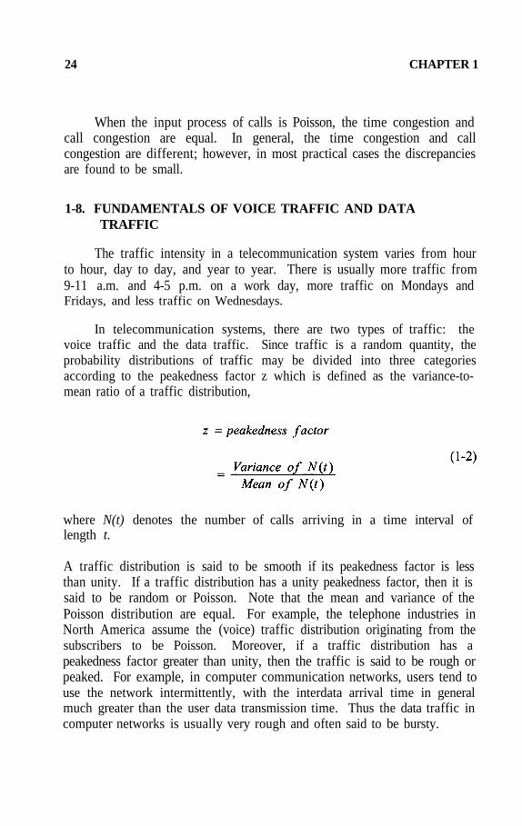
In telecommunication systems, there are two types of traffic: thevoice traffic and the data traffic. Since traffic is a random quantity, theprobability distributions of traffic may be divided into three categoriesaccording to the peakedness factor z which is defined as the variance-to-mean ratio of a traffic distribution,

where N(t) denotes the number of calls arriving in a time interval oflength t.

A traffic distribution is said to be smooth if its peakedness factor is lessthan unity. If a traffic distribution has a unity peakedness factor, then it issaid to be random or Poisson. Note that the mean and variance of thePoisson distribution are equal. For example, the telephone industries inNorth America assume the (voice) traffic distribution originating from thesubscribers to be Poisson. Moreover, if a traffic distribution has apeakedness factor greater than unity, then the traffic is said to be rough orpeaked. For example, in computer communication networks, users tend touse the network intermittently, with the interdata arrival time in generalmuch greater than the user data transmission time. Thus the data traffic incomputer networks is usually very rough and often said to be bursty.

CHAPTER 1 25

A fundamental problem in the design of telecommunication networksconcerns the dimensioning of a route. That is, for a given volume ofoffered traffic and a given grade of service, how many trunk circuits arerequired to interconnect two end offices? What capacity (in bits persecond) should be made available on each link of the network to provide aspecified grade of service for a given volume of offered traffic?

In order to answer the above questions, some statistical informationabout the nature of the offered traffic and the usage of the trunks or linksis needed. In general, the traffic offered to a group of devices (lines,circuits, links, trunks or traffic paths) can be specified by two parameters:

1. The average arrival rate that is, the average calling rate in calls perhour for voice traffic, or the average message arrival rate in messagesper second for data traffic.

2. The average service time that is, the average holding time per callin hours or 100 seconds for voice traffic, or the average transmissiontime per message in seconds for data traffic.

For voice traffic, the calling rate is usually defined as the number of callsper traffic path during the busy hour. The average holding time is theaverage duration of occupancy of a traffic path by a call. For data traffic,the average message arrival rate is the average number of messages persecond arriving at a node for processing. The reciprocal of the average

holding or service time, in calls per hour, is referred to as the

service rate. Moreover, the dimensionless quantity which is the ratio ofaverage arrival rate to the average service rate

is internationally called the erlang, named after A.K. Erlang, the father ofteletraffic theory. This quantity is also called the offered traffic or trafficintensity. One erlang represents a circuit occupied for one hour.

If a group of s trunk lines carried erlangs of traffic, then thecarried traffic per line

26 CHAPTER 1

is called the occupancy of a line, where

Example 1-1. Consider the voice traffic originating from a largenumber of subscriber lines with calling rate, calls/hour. Theaverage holding time of a call is minutes. Calculate (a) the trafficintensity or offered traffic, (b) the occupancy of a circuit if the trafficcalculated in (a) is offered to 10 circuits which encounter a 1% loss, and(c) the peakedness factor.

Solution. (a) The calling rate is calls/hour and the averageholding time is minutes. Thus the traffic intensity or offered trafficis given by

(b) The carried traffic is

Hence occupancy of a circuit is

(c) Since the number of subscriber lines is large, we may assume that theoriginating traffic is Poisson with calling rate According to the theoryof probability (see Example 4-1), it is known that the Poisson distributionhas equal mean and variance. This implies that if N(t) denotes the numberof calls originating in a time interval of t time units long, then

Therefore, using (1-2) we find the peakedness factor

CHAPTER 1 27

In the analysis and design of telecommunication systems, busy-hourtraffic data are commonly used. Traditionally, the design of telephoneswitching centers is based on the traffic intensity during the busy hour inthe busy season. In teletraffic analysis, the busy hour is defined as thatcontinuous sixty-minute period during which the traffic intensity is highest.

The concept of the busy hour can be defined in several ways. Thefour most commonly used definitions of busy hour traffic are as follows:

Definition 1. The average of the busy hour traffic on the 10 busiestdays of the year (North American standard).

Definition 2. The average of the busy hour traffic on the 30 busiestdays of the year (defined as the mean busy hour traffic).

Definition 3. The average of the busy hour traffic on the 5 busiestdays of the year (referred to as the traffic on exceptionally busy days.)

Definition 4. The average weekday traffic over one or two weeks ina given busy season (normal practice for manual or operator switchedtraffic).

From the above definitions, we see that the busy hour traffic based ondefinition 1 is greater than the one of definition 2. As a result the designbased on definition 1 would require more equipment than definition 2.

Teletraffic may be defined as the occupancy of certain devices in thenetwork during the process of setting up a connection. Note that traffic isgenerated from the moment the calling subscriber lifts the handset (thetelephone goes off hook), until the call is released by replacing the handsetback on its cradle (the telephone goes on hook).

Traffic Units. The international unit of telephone traffic is theerlang. One erlang represents the occupancy of a device for one hour.Thus one erlang equals one call-hour per hour. Note that the trafficintensity of a channel represents the occupancy or efficiency of thechannel.

Traffic Intensity. Traffic intensity is defined as the product of thecalling rate and the average holding time.

28 CHAPTER 1

When the average call holding time is expressed in hundred seconds,the resulting traffic unit is called hundred-call-seconds or centum-callseconds (CCS). In this case, 1 erlang equals 36 CCS, for there are 36hundred-seconds in 1 hour. The traffic unit CCS is only used in NorthAmerica.

Example 1-2. Consider a group of 1000 subscribers which generate500 calls during the busy hour. The average call holding time is 200seconds. What is the offered traffic in erlang and in CCS?

Solution. The offered traffic of the group is

or

The offered load or offered traffic is also referred to as the traffic intensity.

1-9. OUTLINE OF THE BOOK

In this book, we present the basic concepts and fundamental methodsfor analysis of telecommunication networks and local area networks. Forswitching networks the primary performance measure is the blockingprobability between a pair of inlet and outlet. For telephone networks withPoisson input traffic, such as the Erlang loss and Erlang delay systems, theperformance measures are the blocking probability and the delayprobability, respectively. For local area networks, the main performancemeasures are the average transfer delay for a message traversing thenetwork and the throughput.

Chapter 1 covers a brief historical overview of the development oftelecommunications. After defining some important terms needed for thedescription of telecommunication systems, we describe several typicaltelecommunication networks such as the public telephone network, theARPA network for computer communication, the SITA network for world

CHAPTER 1 29

wide airline reservation service, and the Ethernet for local area networks.In addition, we introduce the concepts of time congestion and callcongestion, the peakedness factor as a basic parameter for thecharacterization of the input traffic in a telecommunication network, andthe busy hour traffic.

Chapter 2 provides the background knowledge of transmissionsystems for telecommunication networks. We present methods forsubscriber loop design and digital transmission, and techniques for signalmultiplexing, and discuss their differences, advantages and disadvantages.

Chapter 3 introduces the basic principles of switching systems,switching techniques and methods of calculation of congestion. We usenetwork graphs and channel graphs to simplify the calculation. Also weinvestigate both the blocking and nonblocking networks.

Chapter 4 provides a detailed study of the modeling techniques oftraffic flows. We point out the important properties of the Poisson trafficflow and the Markov property of the exponential service time distribution.Using the methods of Markov chain and imbedded Markov chain, weinvestigate the M/M/1 queue, the M/G/1 queue, and the GI/M/1 queue indetail. We determine the state probability distributions for the M/M/1 andGI/M/1 queues and for the birth and death process, which forms a basicmodel for the study of congestion in telephone systems. Furthermore, wederive the Pollaczek-Khinchin formula for mean waiting time for theM/G/1 queue and also formulas for the average transfer delay in theM/G/1 queue with vacation and with priority discipline.

Chapter 5 investigates the Erlang loss and Erlang delay systems asthe central models for the design of telephone systems in North America.Using the result obtained from the birth and death process, we derive twoformulas for the calculation of congestion in telephone systems. Theseformulas are known as the Erlang B and the Erlang C formulas. Inaddition, we determine the waiting time distribution for the Erlang delaysystem with service in order of arrival. We also study the overflow inalternate routing networks and present the equivalent random method foranalysis and design.

Chapter 6 treats the Engset loss and Engset delay systems withquasi-random input. These systems form the primary models for thedesign of telephone systems in Europe. By means of the result obtained

30 CHAPTER 1

from the birth and death process, we determine two formulas for thecalculation of congestion in telephone systems. These formulas are knownas the Engset loss and Engset delay formulas.

Chapter 7 introduces the fundamentals of local area networks with abus structure. For simplicity of analysis we assume the data traffic to bePoisson. We discuss three multiaccess techniques for controlling theaccess to the transmission medium on the network: fixed assignment,random assignment, and demand assignment. We then calculate theaverage transfer delay and throughput for all three multiaccess methods.

Chapter 8 presents the basic features and the two modes of operationin polling networks as well as their configurations. Having described theoperation of a bus polling network with either roll-call polling or hub-polling, we examine the polling cycle and the average waiting time. Thenwe develop an expression for the average waiting time of the packet for anexhaustive network, partially gated network, and gated network. Finally,we obtain an expression for the average transfer delay in terms of theaverage waiting time.

Chapter 9 provides an investigation of the performance of token ringnetworks for multiple-token operation, single-token operation, and single-packet operation. After introducing the concepts of ring latency and stationlatency, we develop expressions for the average transfer delay for theabove three operations.

A basic problem in the design of slotted ring networks is to adjust thenumber of slots so that the gap is minimized. If the station latencies arenot sufficient for the required ring latency, artificial delays can be added inthe station latency.

We show that the throughput can be increased by allowing multiplepackets on the register insertion ring network. For the performanceanalysis of register insertion ring networks, a simplified model isemployed. In this case, the maximum throughput can be greater thanunity. The average transfer delay is shown to be the same for both thering priority and station priority schemes.

Chapter 10 investigates the performance of slotted ALOHA networksfor cases of Poisson input and a finite number of stations. For the lattercase, we present a Markov chain analysis for the study of the dynamic

CHAPTER 1 31

behaviour of the slotted ALOHA network. Moreover, we discuss ananalytical technique called equilibrium point analysis for the investigationof more complicated protocols.

We also carry out the performance analysis for both the carrier-sensemultiple access protocols and carrier-sense multiple access with collisiondetection protocols under the assumption that propagation delays are muchsmaller than the packet transmission time. By means of carrier-sense, thethroughput can be increased.

1-10. SUMMARY

This chapter gives a perspective on telephone networks, local areanetworks and computer communication networks. We define a number oftechnical terms pertinent to the understanding of the structure and operationof telephone and computer communication networks.

A telecommunication network can be viewed as a communicationnetwork which consists of a transmission subnetwork, a switchingsubnetwork, and a signaling subnetwork. These three subnetworks interactand function in a specific and cooperative way to provide good quality ofservice for communications.

To simplify network operation and management, two types ofhierarchical telephone networks, the AT & T and the ITU-T (or CCITT)networks, were established to serve all the countries in the world. Moderntrends in telecommunications are to establish a universal communicationnetwork known as the broad band integrated services digital network (B-ISDN) which can handle voice, data, video and image traffic. Theinternational standard for this network is named asynchronous transfermode (ATM).

It is well known that the call arrival process to a telephone network isa Poisson process with a constant arrival rate and that the data traffic isbursty. However, the bursty nature of data traffic is not well understoodand requires much research.

32 CHAPTER 1

REFERENCES

[1] Keshav, S., An Engineering Approach to Computer Networking,Reading, Mass.: Addison-Wesley, 1997.

[2] Flood, J.E., Telecommunication Networks, editor, Herts, England:Peter Peregrinus Ltd., 1975.

[3] Talley, D., Basic Electronic Switching for Telephone Systems,Rochelle Park, N.J.: Hayden Book, 1975.

[4] Martin, J., Telecommunications and the Computer, 2nd ed.,Englewood Cliffs, N.J.: Prentice Hall, 1976.

[5] Briley, B.E., Introduction to Telephone Switching, Reading, Mass.:Addison-Wesley, 1983.

[6] Boucher, J.R., Voice Teletraffic Systems Engineering, Norwood,M.A.: Artech House, 1988.

[7] Grunn, H.J., Principles of Traffic and Network Design, Geneva, I1.:abc TeleTraining Inc., 1986.

PROBLEMS

1-1. What is the difference between a primary high usage trunkgroup and an intermediate high-usage trunk group?

1-2. What is the grade of service for a telephone network?1-3. What is the difference between the concepts of time congestion

and call congestion?

1-4. Suppose that a data traffic distribution has a mean of 10messages per second and a standard deviation of 7 messages persecond. What is the peakedness factor of this data traffic?

1-5. Poisson traffic originates from 10,000 subscribers with a rate of500 calls per hour. The average holding time of the calls is 2.5minutes. (a) What is the offered load? (b) If the Poissontraffic is served by 25 circuits with a 2% loss, what is thecarried load? (c) What is the occupancy of a circuit?

CHAPTER 2

TRANSMISSION SYSTEMS

2-1. INTRODUCTION

The primary function of a transmission system is to provide circuitshaving the capability of accepting electrical signals at one point anddelivering them to a distant point with good quality. A transmissionsystem in its simplest form may be a pair of wires connecting twotelephones. In a telephone network, a call between two distant points canbe set up by connecting a number of transmission systems in series to forma communication path between the two points. The telephone set convertsthe acoustic signal (voice) into an electrical signal. It also converts areceived electrical signal to its corresponding acoustic form. In addition, itgenerates supervising signals (on-hook and off-hook) and the addressinformation for the switching system to establish connections.

A Simple Telephone Connection. A connection between twotelephones requires two wires as shown in Figure 2-1 (a). If the distancebetween the two parties is substantial, it may be necessary to use amplifiers(repeaters) to compensate for signal attenuation. Since amplifiers are uni-directional devices, for two-way communications it is necessary to use afour-wire transmission, as shown in Figure 2-l(b). However, the switchingequipment in the local office and the local loops on the premises aredesigned for only two-wire operation. Thus, we must convert the locallyused two-wire circuits to the four-wire circuits used for long distancetransmission. This conversion is accomplished by a hybrid coil (or hybridtransformer), as shown in Figure 2-l(c). The rules of operation for thehybrid transformer are that signals entering at A only go to C but not toB, while signals entering at C only go to B but not to A .

Twisted Pair Cable. A twisted pair is made by twisting twoinsulated conductors together. The wire pairs are stranded in units, and theunits are then cabled into cores. Common wire sizes used are 19-, 22-,24-, and 26-gauge.

The characteristics of a pair cable are determined by the primaryconstants: R, the series resistance in ohms per unit length; L, the seriesinductance in henries per unit length; G, the shunt conductance in Siemens

34 CHAPTER 2

per unit length; and C, the shunt capacitance in farads per unit length.These primary constants are functions of the frequency: only C isrelatively independent of the frequency; G is generally small; L decreasesto about 70 percent of its initial value as the frequency increases from 50kHz to 1 MHz and is stable beyond; and R, relatively constant over thevoice band, is proportional to the square root of the frequency at higherfrequencies due to the skin effect.

CHAPTER 2 35

Wire pairs may be used to transmit both analog and digital signals.The most common use of wire pairs is for the transmission of voice. If acircuit uses a separate transmission path for each direction, the circuits arecalled channels. Digital signals may be transmitted over an analog voicechannel by using a modem. Analog signals may be sent over a digitalchannel by using analog-to-digital conversion.

The Transmission Line. Consider a transmission line consisting of a paircable as shown in Figure 2-2. Analog signals may be sent over a digitalchannel by using analog-to-digital conversion.

Since and we can write the differential equations

where

and

36 CHAPTER 2

Using the conditions at the receiving end of the line, namely, whenand the solutions to the above differential equations are

given by

and

where

and

The characteristic impedance approaches a constant value of athigh frequencies. The significance of characteristic impedance is that whena transmission line is terminated in its characteristic impedance, any signalon the line is absorbed when it reaches the terminating resistance. Thusthere are no reflections. The propagation constant represents theattenuation in nepers per unit length, and the phase shift in radiansper unit length.

CHAPTER 2 37

By examining the propagation constant at various frequencies, weshall consider the approximate value for α in four different cases: thefrequencies and the frequencies

the frequencies and andhigher frequencies.

Case 3. If and then neglecting the termswith G and using the approximation

the value of attenuation reduces to

Case 4. If the frequency is higher than that of Case 3, then R isproportional to due to the skin effect and hence is proportional to

Note that the attenuation α is proportional to for both cases 2 and4. For most practical applications, twisted pair cables are used in thefrequency range of Case 2. Typical values of the primary constants for a0.63 mm diameter copper twisted pair are:

38 CHAPTER 2

However, attenuation is not the dominant effect of the operatingfrequencies of twisted pairs. The most important effect is the crosstalk,caused by the shunt capacitance between pairs in the same cable. Theeffect of crosstalk can be reduced by complicated balancing networks ofresistors and capacitors at each end of the cable. Nevertheless, crosstalkimposes a practical upper limit of 500 kHz on operating frequencies. Atfrequencies of 1 MHz or higher, coaxial cables may be used in order toovercome the crosstalk limitations of twisted pairs.

A Simple Transmission Scheme. Since the internal impedance of amicrophone is much less than that of the line, greater power transfer intothe telephone line may be achieved by the use of a transformer, as shownin Figure 2-3(b). Because of the necessity of service and replacement, it ismuch more economical to use a large central battery of -48V at the localexchange. Figure 2-3(c) shows a method of feeding the direct current intothe line. An auto-transformer is used in the instrument to match theimpedances and a capacitor is used to prevent the direct current flowingthrough the receiver. For signaling purposes, two equal inductors are usedto prevent the battery from producing a shunt on the signaling path. Theseinductors are part of a relay for signaling use.

Local Telephone Networks. A local telephone network includes thefollowing components:

1. The subscriber plant;

2. The local exchanges (central offices);

3. The trunk plant connecting local exchanges and those trunksconnecting local exchanges to the next level exchange of networkhierarchy (Class 4 exchanges or toll centers);

CHAPTER 2 39

40 CHAPTER 2

4. The class 4 exchanges (USA) or the primary centers (CCITT).

For a given quality of service, in order to build the most economicallocal network, certain constraints will have to be placed on the design.Important information required for the design includes:

• Geographic extension of the local area under consideration;

• Number of inhabitants and existing telephone density;

• Calling habits;

• Percentage of business telephones;

• Location of existing telephone exchanges and extension of theirserving area;

• Trunking scheme;

• Present signaling and transmission characteristics.

For the study of local telephone network design, we shall assumethat:

• Each exchange will be capable of serving up to 10,000subscribers;

• All telephones in the area have seven-digit numbers, the last fourof which are the subscriber number of the respective serving areaof each exchange;

• All subscribers are connected to their respective exchanges by wirepairs.

2-2. SUBSCRIBER LOOP DESIGN

The subscriber loop (the pair of wires connecting the subscribertelephone set to the local end office) is a dc loop powered by a battery of-48 V. It provides a metallic path for:

CHAPTER 2 41

• The talk battery for the telephone transmitter;

• An ac ringing voltage for the bell on the telephone;

• A current to flow through the loop when the telephone instrumentis taken out of its cradle (off hook), informing the switch of theneed for service and thus causing a line seizure at that switch;

• The telephone dial that, when operated, makes and breaks the dccurrent on the closed loop, indicating to the switching equipmentthe called party number with which communication is desired.

When designing subscriber loops, we must deal with the twolimiting factors on their length: attenuation and IR drop. Here attenuationrefers to energy loss in the line at a reference frequency, measured indecibels. The reference frequency is 1000 Hz in North America and 800Hz in Europe. As a telephone loop is extended in length, its loss at thereference frequency increases. Thus, at some point as the loop is extended,the subscriber cannot hear sufficiently well because of attenuation.Likewise, as the loop is extended in length while the battery (supply)voltage is constant, the effectiveness of signaling is decreased. Thislimit is due to the IR drop of the line. When a telephone is taken offhook, the telephone loop is closed and a current flows, closing a relay atthe local exchange. If the current flow is insufficient, the relay will notclose or will close and open intermittently (chatter) such that line seizurecannot be effected.

Suppose that the following limits are specified for a subscriber loop:

2-2-1. Basic Resistance Design. The formula for calculating the dcloop resistance for a copper conductor is

42 CHAPTER 2

where is the dc loop resistance in per kilometer and d is thediameter of the conductor in millimeters.

For a given loop length of, say, 10 km, the dc loop resistance iscalculated by the formula

or for a given dc loop resistance of a wire, the maximum subscriber looplength can be expressed as

where the loop length is defined as the distance from the subscriber to thecentral office.

Thus,

Table 2-1 lists the diameter and dc loop resistance for severalsubscriber cables of which the sizes of 19-, 22-, 24-, and 26-gauge are themost commonly used.

The diameter of copper wire required is then equal to

From the American wire gauge (Table 2-1), we see that a 22-gauge wire isrequired. Note that the wire resistance in (Table 2-1) must bedoubled for the loop resistance in since there is a go and returnpath in a loop.

CHAPTER 2 43

If the size of the gauge wire is given, we can determine themaximum loop length for a given signaling resistance from a loss andresistance table typified in Table 2-2.

For a 26-gauge loop and a 1250 loop resistance limit, themaximum permissible loop length is

This method of determining the maximum subscriber loop length using thesignal resistance limit as a basis is called the basic resistance design.

44 CHAPTER 2

Example 2-1. Consider a subscriber loop 10 km long. The dc loopresistance limit is assumed to be 1250 Calculate the dc loop resistanceand determine the cable gauge for the loop.

Solution. The dc loop resistance is given by

The diameter of the conductor is given by

Using Table 2-1, we find that a 22-gauge cable should be used.

2-2-2. Basic Transmission Design. The maximum permissible looplength may also be determined using the attenuation or loop loss as a basis.The formula for calculating the maximum permissible loop length is givenby

For a 26-gauge loop and a 6 dB loss, the maximum permissible looplength is

CHAPTER 2 45

This method of determining the maximum subscriber loop length using theattenuation limit (loop loss) is called the basic transmission design.

Example 2-2. Calculate the maximum subscriber loop length for a22-gauge cable with an attenuation limit of 6 dB.

Solution. For a 22-gauge cable, the loss per kilometer is 1.05 dB/km(see Table 2-2). The maximum permissible loop length is

Comparing this result with that of Example 2-1, we see that in thisparticular example the attenuation limit is more severe than the signalresistance limit.

If a 22-gauge cable with H-66 type of loading is used, then we seefrom Table 2-4 that the attenuation is reduced to 0.56 dB/km. In this case,the maximum permissible loop length is extended to

However, the diameter of the 22-H-66 cable has a loop resistance of 110and only has a dc loop resistance of 1178 Therefore, using a

22-H-66 cable will satisfy both the AC loss limit and the IR drop limit.

In many situations, it is desirable to extend subscriber loop lengthsbeyond the permissible limit without increasing the conductor diameter.Common methods involve the use of amplifiers and/or loop extenders, aswell as inductive loading coils.

A loop extender is a device that increases the battery voltage on aloop and hence extends its signaling range. It may also contain anamplifier, thereby extending the transmission loss limit as well.

46 CHAPTER 2

Inductive loading consists of inserting series inductances (loadingcoils) into the loop at fixed intervals. This will reduce the transmissionloss on subscriber loops.

Loaded cables are coded according to the spacing of the loadingcoils. The standard code for loading coils regarding spacing is shown inTable 2-3. The most commonly used spacings are B, D, and H.

When determining signaling limits in subscriber loop design,approximately 15 per loading coil should be added, as if the coils wereseries resistors.

Table 2-2 is useful for the calculation of attenuation of loaded loopsfor a given length. For example, for a 6 dB attenuation limit, themaximum permissible loop length using a 19-gauge wire is

However, using a 19-H-88 loaded cable, the maximum permissible looplength is extended to

CHAPTER 2 47

Table 2-4 shows more properties of cable conductors, where loadingarrangement code 19-H-88 indicates: the number 19 denotes the 19-gaugewire; H indicates the spacing between coils; the number 88 refers to theinductance (in milli-henries) of the coils.

Both the transmission limit and the signaling limit can be extended ata cost. If the pairs to be extended are few, they should be extended.However, if the pairs to be extended are many, it may be more economicalto set up a new exchange area. The current tendency is to reduce the wiregauge where possible.

The size of an exchange area depends on the subscriber density, thesubscriber traffic, and its distribution. Exchange sizes are often in units of10,000 lines. Ten thousand is a convenient number which has importantsignificance in telephone numbering. Consider a seven-digit number, say,284-5000. The first three digits identify the local exchange, and the lastfour digits identify the individual subscriber line and is called thesubscriber number. For a four-digit subscriber number, there are 10,000numbers, from 0000 to 9999. Also 10,000 lends itself to crossbar switchunit size and is an average unit for subscriber densities in suburban areasand midsized towns in fairly well-developed countries. The term wirecenter is often used to denote a single location housing one or more10,000-line exchanges. Some wire centers house up to 100,000 lines witha specific local serving area.

Various gauges of cables may be combined to provide goodtransmission with minimum plant cost. Figure 2-4 shows that customerswithin 15 kft of the central office are served with all 26-gauge nonloadedcables. Those between 15 and 18 kft are served with loops made up ofpartly 26-gauge and partly 24-gauge. Beyond 18 kft, inductive loadingmust be added. Customers between 40 and 50 kft are served with acombination of 19- and 22-gauge. In general, the longer the loop, thecoarser the gauge that must be used.

Loaded Cable Circuits. Loading coils are used in telephone cablecircuits. They have a resistance of a few ohms and an inductance of 10-100 milli-henries. They introduce lumps of inductance into the line atfixed intervals. These loading coils tend to enhance voice transmission

48 CHAPTER 2

CHAPTER 2 49

quality within the 0 to 4 kHz voice band.

Loading coils provide a means of introducing a fairly large amount ofinductance into a line. The coils are placed on the line at distances notmuch greater than a quarter-wavelength of the higher frequency transmittedso that the practical effect is much the same as if the distributed inductancewere increased. Loading coils, acting with the capacitance and inductanceof the line, constitute a low-pass filter. Thus, a line with loading coils willnot transmit the frequencies required for carrier-current transmission. Animportant practical effect of loading coils on the line is that thecharacteristic impedance is increased, and becomes more nearly resistiveand more nearly uniform over the range of frequencies transmitted. Thishelps with impedance matching. Loading also tends to equalize thevelocity of propagation at different frequencies, which tends to avoid delay

50 CHAPTER 2

distortion.

Figure 2-5 shows the marked reduction of attenuation of transmittedfrequencies that results from loading and the increase of attenuation as thecut-off frequency is approached.

To show that attenuation is reduced by increasing the inductance of acable, consider an approximation of the attenuation constant at radiofrequencies in (2-5); that is,

This expression shows that an increase in inductance will reduce theattenuation. This is the important practical reason for employing loadingcoil on telephone lines.

Note that if x is the distance between the sending end and thereceiving end of the line, an expression for attenuation on a line that is

CHAPTER 2 51

terminated in its characteristic impedance is

where and represent the sending power and receiving power,respectively. In terms of dB, attenuation is defined by

2-3. UNIGAUGE DESIGN FOR TELEPHONE CUSTOMER LOOPPLANTS

Using the basic resistance design method, customer loops aredeveloped with a maximum conductor resistance of 1300 ohms. In theBell system of the United States of America, in order to use minimumcopper while keeping within the 1300 limit, four standard cableconductor gauges (AWG 19, 22, 24 and 26) are used. For urban andsuburban loops up to 52 kft in length, a systematic approach known as theuniform gauge or unigauge design has been developed. This approachtreats the entire loop as one system including the local switchingequipment, the outside plant, and the telephone set. It is capable ofincreasing the transmission, signaling, and supervisory range of localswitching equipment from 1300 to 2500 thus permitting the exclusiveuse of 26-gauge conductors for all loops within 30 kft of the wire center.

Consider a typical layout of a subscriber plant based on the unigaugedesign (Bell system). It can be seen from Figure 2-6 that subscriberswithin 15 kft (5 km) of the switching center are connected over loopsmade up of 26-gauge nonloaded cable fed with the standard -48V battery.These loops are referred to as short unigauge loops. This length rangeincludes 80% of all Bell system main stations. All loops in the 15 to 30kft range are referred to as long unigauge loops, which are also servedover 26-gauge nonloaded cable but require a range extender in the centraloffice. This range extender provides 72V for signaling, an adequatetransmitter current, and a 5 dB midband gain for speech. To extend theloop to 30 k f t , 88 mH loading coils are added at 15 kft and 21 kft

52 CHAPTER 2

points. Loops measuring more than 30 kft long may also use theunigauge principle and are referred to as extended unigauge.

It should be noted that the long 15 kft nonloaded sections, intowhich the switch faces, provide a uniform impedance for all conditionswhen an active amplifier is switched in. This is an important factor withregards to stability.

The unigauge application is particularly attractive in wire centerserving areas that have the following characteristics:

• Extensive requirements for additional cable pairs in the 15-30 kftrange;

• Low requirement for party-line service;

• Low requirement for PBX and special service lines.

2-4. SIGNAL MULTIPLEXING

In telecommunication systems, it is almost always the case that thecapacity of the transmission medium exceeds that required for thetransmission of a single signal. To make cost-effective use of thetransmission system, it is desirable to use the medium by having it carryseveral signals simultaneously.

Multiplexing in transmission systems is a means of utilizing the sametransmission medium for many different users concurrently. There areseveral ways in which signals can be multiplexed, the most important onesbeing space-division multiplexing, frequency-division multiplexing, andtime-division multiplexing.

2-4-1. Space-Division Multiplexing. Space-division multiplexing isthe grouping of many physically separate transmission paths into acommon cable. A telephone cable consisting of hundreds (or thousands) oftwisted pairs constitutes a space-division multiplexed system since manyconversations can be carried on the single cable.

It should be emphasized that space-division multiplexing is notlimited to voice-frequency circuits. In fact, many high-capacitytransmission systems using either frequency or time-division multiplexing

CHAPTER 2 53

can also be space-division multiplexed. For example, a carrier system mayput thousands of message channels on a single coaxial line that is in turnpart of a large cable containing many coaxial lines.

2-4-2. Frequency-Division Multiplexing. In frequency-divisionmultiplexing (FDM), each channel of the system is assigned a fixedseparate segment of the total bandwidth of the transmission medium. Thesignal spectrum for each user’s signal is shifted into the proper bandwidthslot through modulation. Thus, many narrow bandwidth channels can beaccommodated by a single wide bandwidth transmission system.

54 CHAPTER 2

To separate the signals at the receiving end, band-pass filters, one foreach channel, are required so that each channel will be shifted back to theoriginal frequency spectrum.

2-4-3. Time-Division Multiplexing. Time-division multiplexing(TDM) is the sharing of a common transmission medium in time. TDMhas often been used in telephone communications. For example, mosttelephones are in use only a small portion of the time. Thus, severaltelephones can time share a common line to the nearest central office.

If the sharing of the transmission medium or multiplexing is carriedout by a deterministic, sequential allocation of time slots to each user, themultiplexer, transmitter, and receiver operate like a pair of synchronizedswitches. This type of multiplexing is also called synchronous time-division multiplexing (STDM). The time slots are often organized intoframes so that each user is allocated a time slot in each frame. As a resultof the fixed allocation of time slots, channel capacity is wasted if a userdoes not have a message to transmit in the allocated time slot.

Utilization of the shared channel can be significantly increased bycombining a number of signals into a central buffer and transmittingthrough the shared channel. This technique of multiplexing is referred toas asynchronous or statistical time-division multiplexing (ATDM). Figure2-7 shows a schematic diagram of a statistical multiplexer. ATDM allowstime slots to be allocated dynamically. An ATDM system assigns a timeslot only when a source becomes active. A time slot is eliminated when therespective source becomes inactive. Thus an ATDM system periodicallyredefines the length of its frame to change the number of time slots, andhence the number of channels. Circuit-switched telephone networks usesynchronous TDM whereas data networks use asynchronous TDMtechniques.

Each user has a short-term buffer to store input messages. Thesebuffers are polled by a scanner that transfers messages from the linebuffers into a central buffer. Since messages from all user inputs aremixed on the shared channel, each message must be given an identificationfor its destination.

Now it is appropriate to distinguish between multiplexing andconcentration. Multiplexing generally refers to static channel allocationschemes in which given frequency bands or time slots on a shared channel

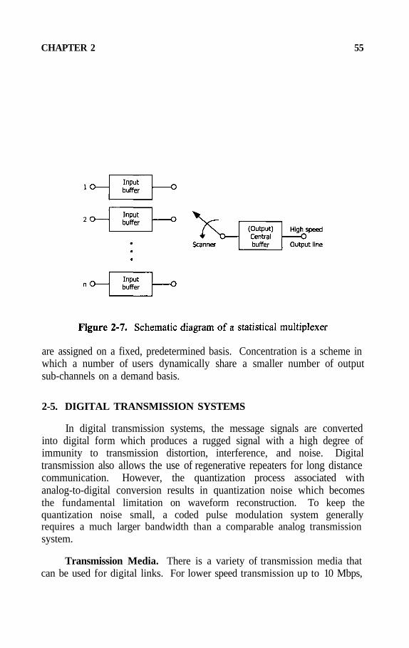
CHAPTER 2 55

are assigned on a fixed, predetermined basis. Concentration is a scheme inwhich a number of users dynamically share a smaller number of outputsub-channels on a demand basis.

2-5. DIGITAL TRANSMISSION SYSTEMS

In digital transmission systems, the message signals are convertedinto digital form which produces a rugged signal with a high degree ofimmunity to transmission distortion, interference, and noise. Digitaltransmission also allows the use of regenerative repeaters for long distancecommunication. However, the quantization process associated withanalog-to-digital conversion results in quantization noise which becomesthe fundamental limitation on waveform reconstruction. To keep thequantization noise small, a coded pulse modulation system generallyrequires a much larger bandwidth than a comparable analog transmissionsystem.

Transmission Media. There is a variety of transmission media thatcan be used for digital links. For lower speed transmission up to 10 Mbps,

56 CHAPTER 2

twisted pair cables are the most commonly used. For higher speeds up to1,000 Mbps, coaxial cables, microwaves, waveguides, and optical fibersmay be employed.

Twisted pair cables and coaxial cables have larger attenuations athigh frequencies. In addition to attenuation, twisted pair cables suffer fromcross-talk caused by electromagnetic coupling between physically isolatedcircuits.

A circular waveguide provides good transmission bandwidth and lowattenuation. Optical fibers provide still larger transmission capacity andlow transmission loss. Microwave systems have been extensively used forfrequency-division-multiplexed analog signals as well as for transmittingdigital signals by modulating a carrier.

The block diagram of a digital baseband transmission system isshown in Figure 2-8. With the exception of local area networks limited toa few kilometers at maximum, most data transmission links make use oflines of the public switched telephone networks. These lines haverelatively well-defined characteristics.

Table 2-5 summarizes typical capacities for transmission linktechnology.

CHAPTER 2 57

A digital transmission system may consist of a transmitter, atransmission channel (medium), and a receiver which contains an equalizer,a detector, and a clock (timing) recovery device. The main task of adigital transmission system is to transfer a digital signal from the source tothe destination. A digital signal is an ordered sequence of symbolsproduced by a discrete information source. Because of the finite bandwidthof the system, there is an upper limit for the signaling rate. In addition,distortion and noise can cause errors to the transmitted digital signal.Thus, signaling rate and error probability play important roles in theperformance of digital transmission systems.

The function of the transmitter is to provide a transmittable signalthat accurately represents the source information and is matched to thecharacteristics of the transmission channel, the interference, and thereceiver. The transmitter also supplies the required transmitted power.

In general, the characteristics of the transmission channel are time,frequency, amplitude, and temperature dependent. Therefore thetransmitted signal is always distorted during transmission via the channel.Also, interference such as cross-talk and noise are imposed on thetransmitted signal.

For theoretical analysis, the noise amplitude X is often assumed to beGaussian with zero mean and variance that is, the noise amplitude isrepresented by a Gaussian (or normal) random variable with the probabilitydensity function

58 CHAPTER 2

For polar binary signals with positive or negative pulses of amplitudeor with equal probability, an error occurs if the noise is more

negative than when the pulse is positive, or if the noise is morepositive than when the pulse is negative. Thus the error probabilitycan be expressed as

By making a change of variable, the integral term can bewritten as

Hence

CHAPTER 2 59

The integral term in (2-14) is known as the error function and isoften denoted by

Furthermore, the quantity is called the complementary errorfunction and is denoted by

Thus, in terms of the complementary error function, (2-14) can beexpressed as

This formula is useful in determining the probability of decision error indigital transmission.

If the transmission of pulses can take on any of m amplitude levelswith equal probability, then the separation between levels israther than for polar binary signals. Consequently, an error will occurif the magnitude of the noise at the decision time is greater than

In this case, the formula for determining the error probabilityfor polar m -ary signals is given by

Clearly, for formula (2-17) reduces to (2-16).

In digital data communication (analog or digital signal), afundamental requirement is that the receiver knows the starting time andduration of each bit that it receives.

60 CHAPTER 2

There are two schemes for meeting this requirement: asynchronoustransmission and synchronous transmission. Asynchronous transmission isthe earliest and simplest scheme for transmitting messages in separategroups. Within an individual group, a specific predefined time interval isused for each message. However, the durations of transmission of thegroups are unrelated to each other. Thus the sample clock in the receiveris reestablished for reception of each message. Synchronous transmissionis a more efficient scheme of transmitting digital data continually at aconstant rate. Hence the receiver must establish and maintain a sampleclock that is always synchronized to the incoming data.

2-5-1. Asynchronous Transmission. An asynchronous line can bein an idle state or in an active state. The idle state of the line is logical 1.In this scheme, data are transmitted one character at a time. Each characteris preceded by a start bit (a 0) and followed by a stop bit (a 1), as shownin Figure 2-9(a). When there is no data to send, the transmitter sends stopbits continuously. The receiver detects the beginning of a new characterby the transition from 1 to 0 and uses the start bit to synchronize itself tothe bit timing of the incoming signal. To establish synchronization, a clockrunning at 16 times the bit rate is used and the alignment is made to onesixteenth of a bit time.

This scheme works well at low speeds, but at higher rates, providinga 16 times clock can be a difficult problem. Also, transmitting the startand stop bits with every character means that the line utilization is only80% of its maximum. The main attraction of asynchronous transmission isthe ease of determining the sample times in the receiver. Asynchronoustransmission is used only in voiceband data sets (modems) for transmissionrates up to 1200 bps. The major drawback of asynchronous transmission isits poor performance in terms of error rates on noisy lines.

2-5-2. Synchronous Transmission. With synchronous transmission,bits or characters are transmitted without start and stop bits. To allow thereceiver to determine the beginning and end of a block of data,synchronization is required. Here a clock is maintained in the receiverwith the same frequency as the transmitter’s clock and the same phase asthe incoming data. Each block of data begins with a preamble bit patternand ends with a postamble bit pattern. Together, the preamble andpostamble plus the data are called a frame. Depending on whether theblock of data is character-oriented or bit-oriented, there are two types ofpreamble and postamble.

CHAPTER 2 61

With the character-oriented type, each block of data is preceded byone or more synchronization characters, as shown in Figure 2-9(b). Thesynchronization character, called SYNC, is chosen such that its bit patternis completely different from any of the regular characters being transmitted.The postamble is a different character. The receiver detects the beginningof an incoming block of data by the SYNC character and the end by thepostamble character.

The bit-oriented type treats the block of data as a bit stream. Thepreamble-postamble principle is the same, with one difference in that thepreamble or postamble pattern may possibly appear in the data. Toovercome this problem, the procedure known as bit stuffing may be used.For example, the high-level data link control and synchronous data linkcontrol bit-oriented schemes make use of the pattern 01111110 (called aflag) as both preamble and postamble. To avoid the appearance of thispattern in the data stream, the transmitter will always insert an extra 0 bitafter each occurrence of five 1’s in the data to be transmitted. When thereceiver receives a sequence of five 1’s, it examines the next bit. If the bitis 0, the receiver deletes it.

Advantages and Disadvantages of Digital Transmission

An important property of digital transmission is that the noisegenerated in the terminal and the noise encountered in the transmission linecan be separated. Quantization noise generated by the terminal equipmentcan be made smaller by proper choice of the codec (coder-decoder).Because of the regenerative repeater of the digital transmission system, linenoise has little effect on the message signal.

Because the signal-to-line noise ratio requirement is lower in digitalthan in analog transmission, digital transmission often results in betterutilization of noisy media. In cables, digital transmission can provide morechannels at a lower cost than can analog transmission. In radio media,digital transmission can tolerate greater external interference.

In digital transmission, because all signals are in digital form, there iscomplete freedom to intermix them in a common facility. This flexibilitymakes a digital system more useful than an analog system. A majordisadvantage of digital transmission is that much greater bandwidth isrequired.

62 CHAPTER 2

2-6. OPTICAL FIBER TRANSMISSION SYSTEMS

Optical fiber as a transmission medium possesses many specialcharacteristics such as low loss, high bandwidth, small physical crosssection, light weight, electromagnetic interference immunity, and security,which make it very useful for telecommunication systems. When comparedwith coaxial cable, a major advantage of optical fiber is that noequalization is necessary. Also, because of its low attenuation properties,optical fibers can have repeater separation in the order of 10 to 100 timesthat of coaxial cable for equal transmission bandwidth. Optical fiber linksneed regeneration only once every 5000 km or so.

The basic elements of an optical fiber transmission system, as shownin Figure 2-10, are the optical transmitter, the optical fiber, and the opticalreceiver.

CHAPTER 2 63

The optical transmitter consists of a semiconductor light source which maybe a laser diode or a light-emitting diode. The primary function of thelight source is to convert electrical signals (currents) into optical signals(lights). Optical fibers are grouped into two classes: single mode fibersand multimode fibers. Single mode fibers are designed such that only onemode is propagated. Multimode fibers allow the propagation of more thanone mode. In a multimode fiber, each mode travels with a slightlydifferent group velocity. Thus it causes a light pulse to have moredistortion than in a single mode fiber. Single mode fibers have two distinctadvantages. First, single mode fibers have smaller diameter cores. Second,single mode fibers have less internal (Rayleigh) scattering, which reducesattenuation.

As a transmission medium for telecommunication systems, opticalfibers are characterized by two important parameters: attenuation anddispersion. Attenuation, expressed in decibels per kilometer, determineshow far a light signal can travel in a fiber before it must be regenerated.Dispersion, expressed in megahertz per kilometer, is a measure ofdistortion of a light pulse. Dispersion at the receiver end is caused by twofactors: material dispersion and modal dispersion. Material dispersion iscaused by the change in the refractive index of the material with frequency.Modal dispersion arises in multimode fibers due to the fact that differentmodes have different phase and group velocities so that different modesarrive at the receiver at different times. Thus delay distortion (dispersion)will result.

Attenuation. The low attenuation or low transmission loss of opticalfibers has proven to be one of the most important factors in bringing abouttheir wide acceptance in telecommunications.

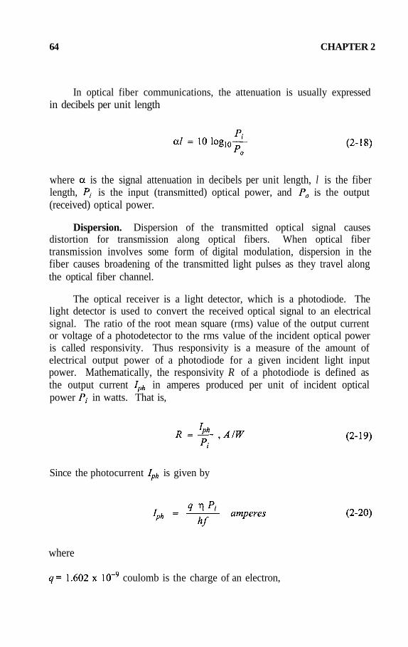
64 CHAPTER 2

In optical fiber communications, the attenuation is usually expressedin decibels per unit length

where is the signal attenuation in decibels per unit length, l is the fiberlength, is the input (transmitted) optical power, and is the output(received) optical power.

Dispersion. Dispersion of the transmitted optical signal causesdistortion for transmission along optical fibers. When optical fibertransmission involves some form of digital modulation, dispersion in thefiber causes broadening of the transmitted light pulses as they travel alongthe optical fiber channel.

The optical receiver is a light detector, which is a photodiode. Thelight detector is used to convert the received optical signal to an electricalsignal. The ratio of the root mean square (rms) value of the output currentor voltage of a photodetector to the rms value of the incident optical poweris called responsivity. Thus responsivity is a measure of the amount ofelectrical output power of a photodiode for a given incident light inputpower. Mathematically, the responsivity R of a photodiode is defined asthe output current in amperes produced per unit of incident opticalpower in watts. That is,

Since the photocurrent is given by

where

coulomb is the charge of an electron,

CHAPTER 2 65

= the quantum efficiency which is the ratio of the average number ofelectrons excited into the conduction band to the number of photons,

J - s is Planck’s constant, and

is the speed of light.

Using the relationship between the wave length and the frequencythe responsivity can be expressed as

where the unit of is in micrometers.

2-7. SUMMARY

The transmission system is the building block of a communicationnetwork. It provides the physical communication links to interconnect thenodes (or transmitting and receiving devices) in a network. The mostcommonly used transmission media for telephone and local area networksare the twisted pair cables and coaxial cables. Because of the relativelyhigh cost, at the current state of technology optical fiber links are suited forpoint-to-point long distance communications.

In the design of subscriber loops in telephone networks, theattenuation due to ac energy loss and IR drop in dc voltage must be takeninto account. These two factors limit the length of a subscriber loop. Wehave presented the basic resistance design and the basic transmissiondesign to determine the maximum permissible length of subscriber loops.To enhance voice transmission quality in telephone networks, loading coilsmay be introduced into the transmission lines at fixed intervals. For urbanand suburban loops, the unigauge design may be employed. This methodpermits the exclusive use of 26-gauge conductors for all loops within 30kft or 9 km of the wire center.

To increase the cost-effectiveness of the transmission system, signalmultiplexing techniques such as space-division multiplexing, frequency-division multiplexing and time-division multiplexing may be employed.

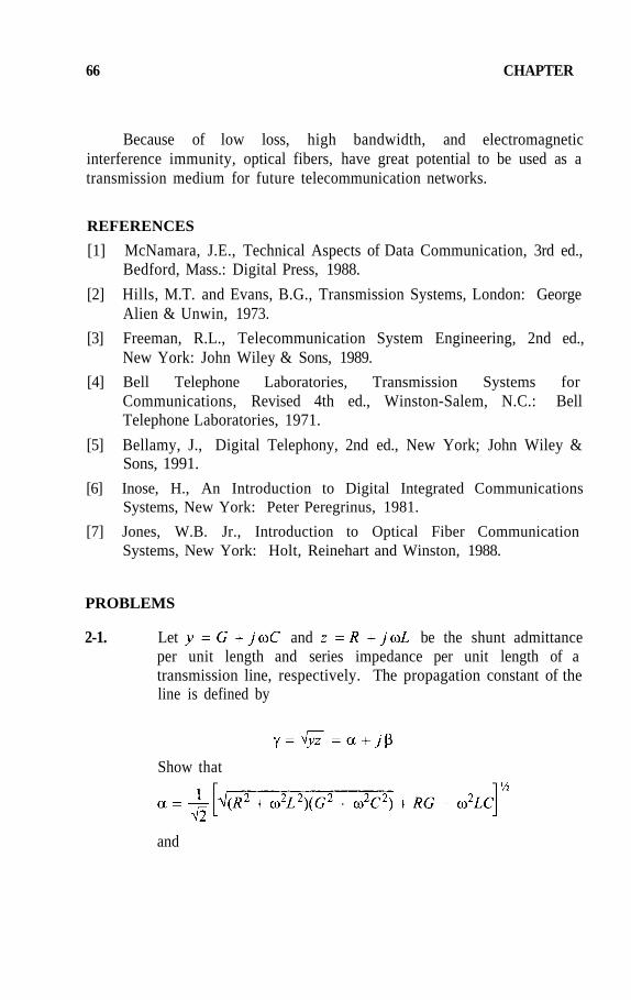
66 CHAPTER

Because of low loss, high bandwidth, and electromagneticinterference immunity, optical fibers, have great potential to be used as atransmission medium for future telecommunication networks.

REFERENCES

[1] McNamara, J.E., Technical Aspects of Data Communication, 3rd ed.,Bedford, Mass.: Digital Press, 1988.

[2] Hills, M.T. and Evans, B.G., Transmission Systems, London: GeorgeAlien & Unwin, 1973.

[3] Freeman, R.L., Telecommunication System Engineering, 2nd ed.,New York: John Wiley & Sons, 1989.

[4] Bell Telephone Laboratories, Transmission Systems forCommunications, Revised 4th ed., Winston-Salem, N.C.: BellTelephone Laboratories, 1971.

[5] Bellamy, J., Digital Telephony, 2nd ed., New York; John Wiley &Sons, 1991.

[6] Inose, H., An Introduction to Digital Integrated CommunicationsSystems, New York: Peter Peregrinus, 1981.

[7] Jones, W.B. Jr., Introduction to Optical Fiber CommunicationSystems, New York: Holt, Reinehart and Winston, 1988.

PROBLEMS

2-1. Let and be the shunt admittanceper unit length and series impedance per unit length of atransmission line, respectively. The propagation constant of theline is defined by

Show that

and

CHAPTER 2 67

2-2. For low-loss lines, the quantities and RG are small and canbe neglected. Calculate (a) the attenuation constant (b) thecharacteristic impedance if the dielectric losses are alsosmall, and (c) the attenuation constant with the additionalcondition as in (b).

2-3. Determine (a) the minimum value of by varying L, and (b)the corresponding phase shift

2-4. Given the values for the primary constants at 100 MHz,and

of a transmission line, can we assume that thisis a low-loss line?

(a) What is the value of the attenuation constant ?

(b) What is the value of the characteristic impedance ?

2-5. A low-loss transmission line which has a capacitanceand an inductance is

operated at radio frequencies. Calculate its characteristicimpedance

2-6. A particular cable operated at high frequencies has a capacitanceof and a characteristic impedance ofWhat is the inductance per kilometer of this cable?

2-7. What is the capacitance per kilometer of a transmission linehaving a characteristic impedance of 417 and an inductanceof 0.54 mH/km?

2-8. What is the maximum subscriber loop length for a 24 AWGloaded cable of diameter 0.511 mm with H–66 loading?

2-9. If the loop resistance limit is 1250 calculate the maximumpermissible loop length for a 26 AWG copper wire.

CHAPTER 3

SWITCHING SYSTEMS

3-1. INTRODUCTION

The purpose of a switching system is to provide a means to passinformation from one terminal device to any other terminal device selectedby the originator. In telephony, switching is used to establish acommunication path between two subscribers. Thus, a switch sets up acommunication path on demand and takes it down when a communicationpath is no longer needed. It performs logical operations to establish thepath and automatically charges the subscriber for usage.

User requirements for a telecommunication switching system may besummarized as follows:

1. The capability of providing a communication path between any twousers;

2. The connection time should be relatively small compared to theholding time or conversation time;

3. The probability of completion of a call should be high, usually 99%;

4. The availability to the user at any time;

5. The primary mode of communication for most users will be voice;and

6. The privacy of user conversation is assumed, but it is neitherspecifically requested nor guaranteed.

Basic Switching Functions. To set up a communication path, a localswitching center must respond to a calling signal originating from aterminal. The switching functions are remotely controlled by the callingsubscriber by off hook, on hook, and dial information. We shall give abrief explanation of each of the basic functions, according to the order ofoccurrence during the progress of a call in a switching system.

70 CHAPTER 3

Attending - When a call is originated from a station or throughanother office, a central office or switching center receives the signal ofrequest for service.

Signal Reception - After receiving the request for service, the centraloffice sends a dial-tone signal to the calling station. Upon receiving thedial information, usually numerical, it responds to address the desiredcalled station.

Signal Interpretation - Based on the received signal information, theswitching office interprets and carries out the required action.

Path Selection - The switching office finds an idle link or series oflinks or channels through the switching center network.

Route Selection - The switching office determines the trunk group towhich a path is to be established; includes intra-office calling.

Busy Testing - This function is to test whether a link or trunk is inuse or reserved for use on another call. When a tested link or trunk isfound busy, successive testing of trunks or links is known as hunting.

Path Establishment - This is the control of the elements of theswitching center network to establish a path for communication. In circuitswitching this function requires some form of memory to retain theconnection for the duration of the call.

Signal Transmission - For inter-office calls, this is the transmissionof the address of the called station to the distant office. Address signalingin station-office communication consists of rotary dial and touch tone.Signaling between telephone offices can be inband or out-of-band using asignal frequency. Moreover, a scheme for communication between thecontrols of central offices is used. This scheme is known as commonchannel inter-office signaling in which the controls of central offices aresent via a private channel.

Alerting - This informs the called station or office that a call is beingsent to it. For intra-office calls, this is known as ringing. For inter-officecalls, it is the transmission of the attending signal.

Supervision - This is to detect when the connection is no longerneeded and to effect its release. Supervision is also required for other

CHAPTER 3 71

purposes such as for call service features, which include call abandonment,no address transmitted, partial address received, unassigned addressreceived, and unequipped address received.

Types of Switching Systems - In telecommunication switching, thereare two principal types of switching known as circuit or line switching andmessage switching or store-and-forward switching.

Circuit Switching - Circuit switching is a form of switching whichsets up a dedicated communication path between two or more stationsthrough one or more intermediate switching nodes. It is also known as lineswitching. Circuit switching can also be applied to a system with aswitching center network that is used for two-way transmission with nochance of transmission delay due to passage through the network. Circuitswitching is widely used in telephone networks. The information may bevoice, data (including telex and teletypewriter), or video.

Store-and-Forward Switching - In this form of switching, messagesare received at intermediate routing points and recorded (stored), checkedfor any errors, and then retransmitted to a further routing point or to theultimate destination. This is also known as message switching. Generally,it implies that no switching center network is employed, but a signal accessnetwork is required. With message switching, it is not necessary toestablish a dedicated path between two stations. Line utilization isincreased. A substantial delay may be produced and may relate to one ofthe following factors:

1. The lack of a common user group of idle transmission facilities at themoment the message reaches the switching office;

2. The need for multiple transmissions of the same message and theneed for storage;

3. The called station or terminal being busy;

4. The speed of message transmission facilities or medium may be lessthan the received rate; or

5. The formatting or coding of the transmitted message being differentfrom the way it was received.

72 CHAPTER 3

The length of delay depends upon the memory capacity provided in aswitching center and the transmission capacity available for use in routingthe message to its destination. In these networks, it is desirable to employswitching memory at the expense of more adequate transmission facilities.

The message may be divided into smaller, usually uniform sizesegments called packets. This form of store-and-forward switching isknown as packet switching. In packet switching, each packet contains dataplus a destination address. If a station has a message to send that is of alength greater than the maximum packet size, the message is broken intopackets for transmission. There are two approaches for the network tohandle the packets: datagram and virtual circuit.

In the datagram approach, each packet is treated independently.Packets with the same destination address do not follow the same route.Thus, it is more flexible and more reliable. It has the advantage that thedelays are shared by all users rather than serving complete messages in theorder of arrival. Thus, many packets of the same message may be intransmission simultaneously, thereby giving one of the main advantages ofpacket switching, namely, the pipelining effect. As a result, thetransmission delay may be reduced considerably (over message switching).At the receiving node, the packets are reassembled to reconstruct theoriginal message.

In the virtual circuit approach, a logical connection is establishedbefore any packets are sent. Each packet now contains a virtual circuitidentifier as well as data. No routing decisions are required at each nodeon the preestablished route. Thus, it differs from the datagram approach.One disadvantage of the virtual circuit approach is that if a node fails, allvirtual circuits that pass through that node are lost.

3-2. CENTRALIZED SWITCHING

In a telephone system serving n subscriber stations, n (n – 1)/2 lineconnections or two-way transmission facilities are required forinterconnection. When every station is interconnected with every otherstation in a telecommunication system, the system is called a meshconnection or a full mesh. An eight-subscriber system, in which eachsubscriber station is directly connected to every other station, is shown inFigure 3-l(a).

CHAPTER 3 73

The switches per station used to select the required connection ofpaths at both ends of the transmission facilities are called crosspoints.Crosspoint is the term more commonly used to denote an electronic circuitthat can electrically connect or disconnect two conductors in response tosome external control signals. A telephone system consisting of n stationswould require n – 1 switches per station and hence in total n(n – 1)crosspoints. Full mesh systems have only limited applications, generallywhere n is small and the traffic levels are comparatively high. These fullyconnected systems are also known as noncentralized switching systems.

From the inception of telephony, the concept of centralized switchingwas realized to be more efficient. A centralized switching network withremote control is shown in Figure 3-l(b). With centralized switching, onlyone two-way line is required per station, but the number of crosspointsremains the same as that of noncentralized switching. The difference isthat for centralized switching the crosspoints must be remotely operated.Centralized switching can be made more efficient in reducing the numberof crosspoints, as shown in Figure 3-l(c), where only n(n – 1)/2 (or halfas many) crosspoints are required. This is known as a single stagenonblocking switching network, which can provide for all stations to beconnected simultaneously without any blocking at all. From Figure 3-l(c),we see that the saving in crosspoints is achieved at the expense ofintroducing the n – 1 links (or lines within the centralized switchingsystem or central office). If fewer than n/2 simultaneous connections arerequired at a given time, then fewer than n(n – l)/2 crosspoints may beused. The number of links required is determined by the desired grade ofservice for a given offered load. In Figure 3-l(d), we may useL < (n – 1)/2 links to further reduce the number of crosspoints. When allthe L links are used for connecting 2L stations simultaneously, theremaining n – 2L stations cannot be connected until one of the L linksbecomes available. Thus, congestion or blocking is always possible.

For a subscriber of one central office to communicate with asubscriber of another central office, call control information (signaling)between central offices is necessary. When more central offices and trunkgroups that connect them are added, it becomes clear that a centralizedswitching office, known as a tandem office in telephony, for central officesis needed (see Figure 3-2).

Typically, an exchange area defined for telephone service will bemade up of a number of local central offices and one or more tandem

74 CHAPTER 3

CHAPTER 3 75

76 CHAPTER 3

offices. The number of trunks between the offices will be based oneconomics to provide the required grade of service.

What we have discussed is the classical network problem of tradingoff between switching and transmission costs to minimize overall costs. Inaddition, certain functions can be located in the tandem office. Forexample, time and weather services may be located in the tandem office toavoid replication in each local office.

3-3. SWITCHING TECHNIQUES

There are three switching techniques based on the division of calls inspace, time and frequency: space-division switching, time-divisionswitching and frequency-division switching.

3-3-1. Space-Division Switching. A network consisting of metalliccontacts is called a space-division network because the communicationpaths set up by the closure of metallic contacts in series are physically

CHAPTER 3 77

separated from each other. The metallic contacts are called crosspoints.They are grouped in a two-dimensional array to form a switch unit. Inspace-division switching, different calls are connected through differentphysical paths separated in space for the duration of a call. A 4 × 4space-division switching is shown in Figure 3-3.

The advantage of space-division switching is its simplicity and goodtransmission properties. For example, the bandwidth of the signal is notunduly limited by the switch mechanism. The disadvantage of space-division switching is that the switches can be relatively slow to operate,can be bulky, and can involve a large amount of wiring because eachconnection needs a separate set of wires.

3-3-2. Time-Division Switching. In time-division switching, all theinlets and outlets are connected to a common transmission path via high

78 CHAPTER 3

speed switches. These switches connect the required inlet and outlet ontothe same path for a short time. Time-division switchings are applicable todigital switching only. Modem large switching systems often consist ofcombinations of time-division and space-division switches.

The signals are time-multiplexed by the switch onto a fast bus, andthe resulting signal is demultiplexed by accurately timed gates inaccordance with the user’s requirements. It uses much less switch pointsthan space-division switching. A typical example using time-divisionswitching in telephony is the pulse-code modulation (PCM) transmission ofvoice samples. Each voice signal is sampled at a rate of 8000samples/second with a sampling period of These samples aredigitized to 8 bits/sample, so that a typical PCM voice channel requires 64kbps of transmission capacity. If 24 8-bit voice channels are multiplexedwith 1 frame bit for each sample, the bit rate is bits/125

This is known as the Tl system. Note that the 24-channel frame can also be used for data transmission.

To carry out time switching, each frame arriving at the switch is firstwritten into a memory. Switching is then accomplished by reading out thestored data in a desired order. Such a device is called a time-slotinterchange (TSI) unit. Time switching may be integrated into digitaltransmission, so that modulation and demodulation take place only at thefar end of the system.

3-3-3. Frequency-Division Switching. As in time-divisionswitching, frequency-division switching also uses a common transmissionpath, but in this case, each signal is modulated onto a different carrierfrequency. Switching is achieved by providing each outlet with ademodulator which can have its carrier frequency changed. Frequency-division switching now finds application in demand-assigned satellitecommunication links. Figure 3-4 demonstrates a simple frequency-divisionswitching. Frequency-division switching can be used to increase the trafficcapacity of the satellite by making all carrier frequencies available to allground stations. Note that the toll telephone network also uses demandassignment.

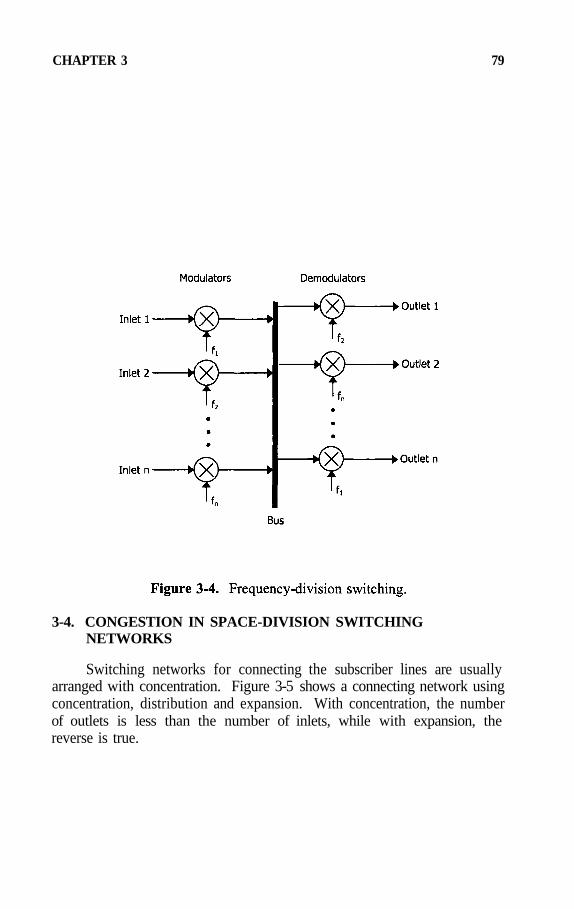
CHAPTER 3 79

3-4. CONGESTION IN SPACE-DIVISION SWITCHINGNETWORKS

Switching networks for connecting the subscriber lines are usuallyarranged with concentration. Figure 3-5 shows a connecting network usingconcentration, distribution and expansion. With concentration, the numberof outlets is less than the number of inlets, while with expansion, thereverse is true.

80 CHAPTER 3

The ratio of the number of inlets to the number of outlets is knownas the concentration ratio. Its value may vary from 2 for high calling rates,to 4 for medium calling rates, and to 6 for low calling rates. Theexpansion ratio is the inverse of the concentration ratio. Its value dependson the loading of the inlets and the desired level of internal blocking. Atypical design for local switching networks is based on an average inletloading of 0.6 erlang and total internal blocking not exceeding 0.002. Tollswitching network dimensions are based on an average inlet loading of 0.7erlang and first trial blocking of 0.005. Distribution (or intermediate)stages are usually arranged without concentration or expansion.

A basic requirement of switching network design is to minimize thetotal number of crosspoints needed to switch a given offered traffic load ata given grade of service. Other factors include complexity of control,flexibility for expansion, and overload performance.

The determination of offered traffic per line is complicated by the factthat an intra-office call occupies two lines, while an outgoing and incomingcall occupies only one line. Similarly, calculations of busy-hour traffic perline must take incoming calls into account. This situation can berepresented in a traffic H diagram as shown in Figure 3-6.

CHAPTER 3 81

In the traffic H diagram, the intra-office traffic is considered as a part ofthe originating traffic. The traffic H diagram is drawn with the assumptionthat the sum of the originating traffic and the terminating traffic is equal tothe sum of the incoming traffic and the outgoing traffic. In North Americathe offered traffic in CCS per line is calculated as the sum of theoriginating traffic and the terminating traffic (which means that the intra-office traffic is counted twice) divided by the number of lines. However,the busy-hour call (BHC) traffic in erlangs per line is calculated as the sumof the originating traffic and the incoming traffic (counting intra-officetraffic only once) divided by the number of lines.

Example 3-1. A switching network in a central office serving 10,000lines has an average origination rate of three calls per hour per line and anaverage holding time of 3 minutes. If the intra-office traffic is 10% of theoriginating traffic and the incoming traffic is 200 erlangs, what are theBHC and CCS traffic per line?

Solution. Since the calling rate per line is 3 calls per hour, the totaloriginating traffic is given by

or

82 CHAPTER 3

The intra-office traffic is equal to

The terminating traffic is the sum of the intra-office traffic and theincoming traffic, that is,

Hence, the BHC traffic per line is given by

and the CCS traffic per line is given by

Note that the BHC traffic per line is equivalent to 0.17 × 36 = 6.12 CCSper line.

3-4-1. Switching Matrices. Switching matrices are used to inter-connect inlet and outlet terminals in a switching network. In the design ofswitching matrices, the number of inlets and outlets, the specified blockingprobability and traffic characteristics, the cost of manufacturing, and thecost of control should be taken into consideration.

For space-division switching matrices, the building block is theswitch array. Figure 3-7 shows a typical switch array for the connection ofn inlets and m outlets (full availability).

CHAPTER 3 83

The one-stage matrix in Figure 3-7 has nm crosspoints. If the trafficoffered per inlet is a erlangs, then the total traffic offered to the switch isna erlangs and the traffic carried per outlet is na/m erlangs which is alsothe occupancy per outlet.

A one-stage square matrix with an equal number of inlets and outletshas the property of nonblocking, because a connection between a free inletand a free outlet can always be made, irrespective of other conditions inthe switch. However, nonblocking switching systems are unnecessarilycostly because terminals are used for only some proportion of the time.Nonblocking switches provide unnecessary switching capacity.

84 CHAPTER 3

3-4-2. Multistage Networks. It is possible to reduce the totalnumber of crosspoints if the switching network is constructed from anumber of stages consisting of smaller matrices. Generally, a switchingnetwork may consist of distribution stages, routing stages, and collectionstages. A distribution stage increases the number of paths from an inlet toan outlet through the network. Corresponding to the distribution stage, acollection stage must be used to collect the distributed paths. A routingstage also increases the number of paths within the network, which has nocorresponding collection stage, so that paths from a routing stage aredirected to different outlets.

To illustrate the idea, let us consider a switching network with 100inlets and 100 outlets. If a one-stage matrix is used, then100 × 100 = 10,000 crosspoints are required. Now suppose that a 10 × 10square matrix is used as the basic building block. One matrix can connectany of 10 inlets to 10 outlets. If each of these 10 outlets is connected to adifferent 10 × 10 matrix, each original inlet can then have access to a totalof 100 outlets. In this case, two crosspoints have to be operated to make aconnection.

This two-stage network introduces a new problem, known as internalblocking. Internal blocking occurs in the two-stage network, because thereis only one link between a particular first-stage switch and each of thesecond-stage switches. If a connection between any pair of first-stage andsecond-stage switches has been made, no further access between that pairwill be possible. Internal blocking is defined as the probability that a freeinlet fails to be connected to a free outlet because of the absence of a freepath (link) between them. The complete arrangement of this two-stagenetwork is shown in Figure 3-8.

The two-stage network in Figure 3-8 consists of a total of twenty10 × 10 basic switches, so that the total number of crosspoints is20 × 10 × 10 = 2,000 instead of 10,000 as in the case of one-stagenetwork.

A larger network can be constructed by adding a further stage.Figure 3-9 shows a construction of a three-stage network with 1000 inletsand 1000 outlets. The first ten 100 × 100 two-stage sub-networks areconnected to 100 separate third-stage switches. These then provide accessto a total of 1000 outlets. The extra inlets on the third-stage switches cannow be used by nine other 100 × 100 two-stage sub-networks.

CHAPTER 3 85

86 CHAPTER 3

Continuing this arrangement for K stages, each stage consisting ofmatrices as basic switches, gives a network with N inlets and N

outlets, where In this general arrangement, each stage ofswitches is called a distribution stage because outlets are distributed overmatrices in the next stage. Note that each stage consists of the samenumber of matrices, N/n.

Example 3-2. Consider the two-stage switching network of N inletsand N outlets. If basic matrices are used, calculate the number ofcrosspoints in the network.

Solution. Since each matrix has crosspoints and there are twostages, each stage consisting of N/n matrices, the total number ofcrosspoints in the network is

crosspoints

For a two-stage network, thus, the network requires a total ofcrosspoints.

Example 3-3. A switching network with N inlets and N outlets isconstructed by matrices. Calculate the optimal size of the matricesused and the number of distribution stages needed for N = 1000 byminimizing the number of crosspoints.

Solution. Let the number of distribution stages be K. Then thenumber of inlets N is related to K and n by the following expression

Thus

Since the number of crosspoints X in a K -stage network is equal to theproduct of the number of stages, K, the number of matrices per stage,N/n, and the number of crosspoints per matrix, then

CHAPTER 3 87

Differentiating X with respect to n and equating to zero gives

or

Hence, the optimal size n of the matrix is

or the optimal size of the basic matrix is

For a 1000-inlet and 1000-outlet network, the required number ofstages will be

For and , this arrangement yields a network ofinlets and 2187 outlets. This network uses a total of

crosspoints. Note that in this analysisthe problem of internal blocking has been ignored. When internal blockingis taken into consideration the optimal arrangement will be based on alarger matrix.

3-4-3. Link Systems. The method of connecting the inlets andoutlets via multistage of matrices is called the link system. A formaldefinition of the operation of the link system is as follows.

1. A connection between an inlet and an outlet in a link system isformed by one or more links;

88 CHAPTER 3

2. The link or links are seized at the same time as the chosen outlet;

3. Only the link or links which connect to the chosen outlet are seized(condition selection).

A switching network may consist of several stages and many linksand paths. In order to calculate the blocking probability, it is convenient touse a diagram known as the network graph to show the pattern of links.In the design and analysis of multi-stage networks, an even simpler graphis drawn for a particular inlet and a particular outlet. This simpler graph isknown as the channel graph.

Network Graph. A network graph of a switching network is agraph in which each switch is represented by a dot and each link by a linejoining appropriate dots in each stage.

Channel Graph. A channel graph of a switching network for aparticular pair of inlet and outlet is a graph in which only the links andintermediate stages that could be used are drawn.

Internal blocking occurs in a link system when there are no idle linksavailable for connection to an idle outlet. A convenient method forcalculating internal blocking in a link system is the linear graph methoddeveloped by C.Y. Lee in 1955. A linear graph, also known as a channelgraph, is a simplified network graph. In order to simplify the calculation ofinternal blocking in switching networks by use of channel graphs, we makethe following assumptions:

1. The occupancy of each link (the fraction of time that a link is in use)of the switching network is independent of other links;

2. The blockings in the basic switches are negligible; and

3. The traffic in the network is conserved.

3-4-3-1. Two-Stage Link Systems. Figure 3-10(a) shows a two-stage link system which uses matrices. Each stage consists of mmatrices and is thus a distribution stage. The corresponding network andchannel graphs are shown in Figure 3-10(b) and (c), respectively.

CHAPTER 3 89

To calculate the internal blocking between stage A and stage B, weassume that the traffic offered per inlet is erlangs. Then the linkoccupancy, which is the traffic carried by a link in the network, is simply

Since there is only one possible path between any A -stage inlet and anyB -stage outlet, the blocking probability is given by

90 CHAPTER 3

If the level of congestion is unacceptable, larger matrices may beused. Suppose that matrices are used, where two parallel paths(interstage links) are available between any A -stage inlet and any B -stageoutlet. In this case, the blocking probability is reduced to

3-4-3-2. Three-Stage Link Systems. Consider the three-stagenetwork depicted in Figure 3-11 (a) with all three stages being distributionstages. The corresponding network and channel graphs are shown inFigure 3-1 l(b) and (c), respectively.

If the traffic offered per inlet is erlangs, the occupancy on anA – B link is

and the occupancy on a B – C link is

Therefore, the blocking probability in a network with three distributionstages is given by

In general, if a network consists of K distribution stages in series, theblocking probability is given by

CHAPTER 3 91

because, for a particular pair of inlet and outlet, there are K – 1 linksconnected in series, each with an occupancy of a. In the derivation offormula (3-6), it has been assumed that the link occupancies in differentstages are independent.

92 CHAPTER 3

Table 3-1 shows the blocking probabilities for networks with differentnumbers of stages and with link occupancies of 5% and 10%, that is,

and 0.1.

From (3-6) or Table 3-1, we see that with an increasing number ofdistribution stages the blocking probability increases. In order to reducethe blocking probability, it is necessary to provide more than one pathbetween each first-stage and last-stage switching matrix.

3-4-3-3. Three-Stage Link Systems Using a Collection Stage.Consider the three-stage link system shown in Figure 3-12(a). The firststage of the network consists of matrices and the second stage,

matrices. Any inlet on the first stage has access to mk B – C links.In order to provide more paths, these mk links are connected to only kthird-stage switches (rather than mk switches, as in a distribution stage).This type of link pattern is called a collection stage. From Figure 3-12(a),we see that the addition of a collection stage to a two-stage network doesnot increase the number of outlets accessible from a first-stage switch, butit does increase the number of paths between switches on the first and laststages.

There are now m possible paths, each consisting of two linksconnecting any inlet on the first stage and any outlet on the last stage.The corresponding network graph and channel graph are shown in Figure

CHAPTER 3 93

3-12(b) and (c), respectively.

If the traffic offered per inlet is then the occupancy on an A – Blink is

94 CHAPTER 3

and the occupancy on a B – C link is

From Figure 3-12(c), the blocking probability is given by

where It will be shown in the next section that a three-stagenetwork becomes nonblocking if

For a three-stage network with and the blockingprobability is which is negligible.

Example 3-4. Consider the switching network whichconsists of K distribution stages. The offered traffic per inlet is a erlangs.Calculate the optimal size of the switches so that the total number ofcrosspoints is minimized.

Solution. Let the size of the switches be By taking thetraffic into consideration, the average number of outlets of the network isreduced to N(1 – a). Similarly, the average number of free linksaccessible from an switch is reduced to n(1 – a). Hence, by takingthe busy links into account, the effective size of a switch appears to be

Therefore, the average number of outlets accessiblefrom a first-stage switch becomes

It follows that the number of stages is given by

CHAPTER 3 95

and the number of crosspoints used in the network is

Differentiating X with respect to n and setting the result to zero yields

or

Suppose that erlangs and Using (3-10) we have

Thus the optimal size of switch is

By (3-9), we obtain the number of stages

Thus the number of stages needed is 6. With and the actualnumber of outlets is

and the number of crosspoints in the network is given by

96 CHAPTER 3

Upon comparison with the result of Example 3-3, we see that by taking thetraffic into account, the size of switches is slightly larger and thenumber of crosspoints is twice as many as when the traffic is notconsidered.

3-5. NONBLOCKING NETWORKS

It is possible to build a multi-stage network in which no internalblocking can occur and which still uses fewer crosspoints than a squarematrix. This problem was solved by C. Clos in 1953 with three stages.Figure 3-13 shows a Clos-type three-stage nonblocking network.

The first stage or A-stage comprises k switches with n inlets each,and the last stage or C-stage comprises k switches with n outlets each.The network has inlets and N outlets. The second stage or B-stagecomprises m switches, each with k inlets and k outlets, so that each Bswitch has one link to each A and C switch.

For nonblocking in stage A, m must not be less than n. However,this condition is insufficient to ensure the absence of blocking in laterstages. Consider the worst possible case for setting up a connection

CHAPTER 3 97

between a pair of inlet and outlet as shown in Figure 3-14. Suppose a freeinlet of switch requires connection to a free outlet of switch If theremaining n–1 inlets of switch are already connected to outlets ofswitches other than switch and the remaining n – 1 outlets of switch

are connected to inlets of switches other than switch thenswitches of stage B are unavailable to the new

call. Hence, the minimum number of switches in stage B to ensurenonblocking is The required nonblocking network then has kswitches in stages A and C, each and 2n – 1 switches instage B, each

98 CHAPTER 3

The total number of crosspoints is therefore given by

where is the number of inlets or outlets of the network. For agiven value of N, the minimum number of crosspoints can be determinedby differentiating X with respect to n and letting it be zero, i.e.

or

Thus, for large N or

Taking the minimum number of crosspoints is approximately

Note that it is possible to construct a 5-stage nonblocking network byreplacing each B switch in Figure 3-13 by a complete 3-stage nonblockingnetwork. In the same way, a 7-stage nonblocking network can beconstructed by replacing each C switch on the third stage in the 5-stagenetwork by a 3-stage network.

CHAPTER 3 99

Example 3-5. Design a three-stage nonblocking network capable ofswitching any of 1000 inlets to any of 1000 outlets. Suppose that the 1000inlets and 1000 outlets are both served by 100 switches. Calculate the totalnumber of crosspoints required.

Solution. Since the number of inlets per A -stage switch is

for the network to be nonblocking, the size of

switches on A -stage is The B -stage has 19 switches, each of sizeThe C -stage is a collection stage consisting of 100 switches,

each of size The complete nonblocking network is shown inFigure 3-15. The total number of crosspoints is

Note that in this simple example, the saving in crosspoints is considerablylarger as compared with the crosspoints in a simple square switch.However, the saving in crosspoints becomes more prominent when N islarger.

100 CHAPTER 3

3-6. THREE-STAGE NETWORKS WITH RETRIALS

If a call is connected to a trunk group, any idle trunk in the groupcan serve the purpose. If the first attempted trunk is busy, then retrialsmay be initiated. This is done by selecting another outlet and reattemptingto make a connection. In most cases, the inlet will make use of the sameset of A – B links but will attempt to match with a different set of B – Clinks as illustrated in the network graph and the equivalent channel graphin Figure 3-16(a) and (b), respectively.

For a call from an inlet to x idle outlets to be blocked, it is necessarythat either the A – B link is blocked, or the A – B link is not blocked butall the x trials failed. This situation is equivalent to that of havingx B – C links, as shown in Figure 3-16(b). The blocking probability is

CHAPTER 3 101

given by

where x is the number of trials, and a and b are the occupancies of the A- B link and B – C link, respectively.

3-7. CONGESTION IN TIME-DIVISION SWITCHINGNETWORKS

Time-division switching is a technique of sharing the crosspoints of aswitch for shorter periods of time so that individual crosspoints and theirassociated interstage links are continually reassigned to existingconnections. It is equally applicable to either analog or digital signals.

To illustrate the basic principle of time-division switching, weconsider the simple analog time-division switching structure shown inFigure 3-17, where a single switching bus is shared by a number ofconnections. The pulse amplitude modulation samples from receive lineinterfaces are interleaved to transmit line interfaces. The first cyclic controlcontrols gating of inputs onto the bus, one sample at a time. The secondcyclic control operates in synchronism with the first and selects theappropriate output line for each input sample. A complete set of pulses,one from each active input line, is referred to as a frame. The frame rateis equal to the sample rate of each line.

The analog switching matrix in Figure 3-17 is essentially a space-division switching matrix. By continually changing the connections forshort periods of time in a cyclic manner, the configuration of the space-division switch is replicated once for each time slot. This mode ofoperation is referred to as time multiplexed switching.

Usually digital time-division multiplexed signals require switchingbetween time slots, as well as between physical lines. This mode ofswitching consists of a second dimension of switching and is referred to astime switching. Figure 3-18 shows the basic requirement of a time-division switching network, where channel 3 of the first TDM link isconnected to channel 17 of the last TDM link. The return connection isrequired and realized by transferring information from time slot 17 of the

102 CHAPTER 3

last input link to time slot 3 of the first link. Thus each connectioninvolves translations in both time and space.

Time Slot Interchange. The time slot interchange (TSI) unit is thebasic building block of many time-division switches. A TSI unit operateson a synchronous TDM stream of time slots, or channels, by interchangingpairs of time slots. This is done by writing data into and reading data outof a digital memory. Figure 3-19(a) shows the basic functional operationof a TSI and Figure 3-19(b) depicts a mechanism for TSI.

The N input lines are synchronously multiplexed to produce a TDMstream with N time slots. To make the interchange of any two slots, theincoming data in a slot must be stored in the memory until they can besent out on the right channel in the next frame cycle. Hence, the TSIintroduces a delay and produces output slots in the desired order. These

CHAPTER 3 103

are then demultiplexed and routed to the appropriate output line. Since theframe must provide a time slot for each channel, the size of the TSI unit

104 CHAPTER 3

must be chosen for the capacity of the TDM line.

TSI is a simple, effective way to switch TDM data. However, thesize of TSI is limited by the memory access speed. Thus, a TSI unit cansupport only a limited number of connections.

Time Multiplexed Switching. For a fixed access speed, as the sizeof the TSI unit grows, the delay at the TSI increases. To overcome theseproblems, multiple TSI units are used. To interchange time slots betweentwo TDM streams of two different TSI units, some form of space-divisionmultiplexing is needed. This operation is known as time multiplexedswitching (TMS).

Multi-stage networks can be built up by connecting TMS and TSIstages: TMS stages, which move time slots from one TDM stream toanother, are referred to as S, and TSI stages are known as T.

To minimize blocking, three or more of these stages are used. Someof the more commonly used structures are: TST, TSSST, STS, SSTSS andTSTST.

The TMS unit must provide space-division connections between itsinput and output lines, and these connections must be reconfigured for eachtime slot.

In an STS network, the path between an incoming and outgoingchannel has a number of possible physical routes equal to the number ofTSI units. For a nonblocking network, the number of TSI units must bedouble the number of incoming and outgoing TDM streams.

Time-Division Switching and Space-Division Switching Analogy.A convenient way for the analysis of traffic flow on multi-stage time-division switching networks is to make use of their space-divisionswitching analogy. Figure 3-20(a) depicts a rectangular time-divisionswitch which connects n incoming and m outgoing lines, each having ktime slots in a frame. In this configuration, a time slot of the TDM streamin any one of the n incoming lines has access to the same time slot in anyone of the m outgoing lines. Thus, the time-division switch isfunctionally equivalent to k separate space-division switches asshown in Figure 3-20(b).

CHAPTER 3 105

Note that no connection between time slots of different frames ispossible with the time-division switch in Figure 3-20(a). However, we canobtain connections between time slots of different frames by connecting then incoming time-division lines to the m outgoing time-division lines byway of r intermediate time-division lines as shown in Figure 3-21 (a). The

106 CHAPTER 3

space-division equivalent of this configuration is shown in Figure 3-2l(b).

With this configuration, there is no distribution between the kequivalent space-division switches. In order to transfer data from one time

CHAPTER 3 107

slot to another time slot, a pulse shifter capable of interchanging anarbitrary time slot at its input to an arbitrary time slot at its output may beemployed. Using pulse shifters in the switch in Figure 3-20(a), thepreassigned time slot in its first time-division stage may be shifted to anyone of the k time slots, so that the network becomes equivalent to a three-stage space-division network as shown in Figure 3-22(a).

Similarly, by employing pulse shifters in the second time-divisionstage in Figure 3-21 (a), we obtain the network shown in Figure 3-23(a).

The networks shown in Figures 3-22 and 3-23 are two basicconfigurations for time-division switching networks. The first configurationis called the T-S-T type and the second configuration is called the S-T-Stype.

Consider the T-S-T (time-space-time) switch in Figure 3-24(a) whichis completely analogous to the three-stage space-division switch in Figure3-12. The corresponding channel graph is shown in Figure 3-24(b).

From the channel graph, we see that there are in total m parallelpaths, each having a blocking probability of where

and is the offered traffic per input channel. It follows thatthe blocking probability is

Note that the crosspoint settings of the space switch are changed, each ofthe m time intervals corresponding to the m time slots of TSIs. Theresultant space switch is called a time-multiplexed switch.

However, practical limitations of memory speed limit the size of a timeswitch, so that some space-division switching is also necessary in largeswitching networks.

Example 3-6. Calculate the blocking probability of the S-T-S switchin Figure 3-25(a) for and the offered traffic per inlet

erlangs.

If the switching network becomes nonblocking.

108 CHAPTER 3

CHAPTER 3 109

110 CHAPTER 3

CHAPTER 3 111

Solution. Since the channel graph for the S-T-S switch in Figure 3-25(b) is exactly the same as that of Figure 3-24(b), formula (3-13) applies.The link occupancy is

Thus, using (3-13) we obtain the blocking probability

112 CHAPTER 3

3-8. SUMMARY

This chapter first presents the basic functions required for publictelephone networks and then discusses the concepts of circuit switchingand store-and-forward switching. Circuit switching is used exclusively inpublic telephone networks and store-and-forward switching is used incomputer communication networks.

For efficient operation and economic reasons, the concept ofcentralized switching with remote control is very useful. However,application of this concept gives rise to the problem of internal blocking inswitching networks. This problem can be solved by trading off betweenswitching cost and transmission cost to minimize the overall cost.

Like signal multiplexing, switching techniques can be divided intospace-division, time-division, and frequency-division switchings. Inpractice, almost all switching networks are multi-stage networks whichconsist of a concentration, a distribution, and an expansion stage and aresubject to blocking with low probability. A typical problem in the designof multi-stage networks is to minimize the number of crosspoints for agiven blocking probability. For nonblocking switching networks, thethree-stage Clos-type of networks may be used.

Under reasonable assumptions, the calculation of blocking in aswitching network can be greatly simplified by the use of network graphsand channel graphs. Several examples are presented for illustration. Inthis respect the method developed by Lee is found to be very useful.

REFERENCES

[1] Hills, M.T., Telecommunications Switching Principles, Cambridge,Mass.: MIT Press, 1979.

[2] Bellamy, J., Digital telephony, 2nd ed., New York, John Wiley &Sons, 1991.

[3] Stalling, W., Local Networks, 3rd ed., New York, MacmillianPublishing Co., 1990.

CHAPTER 3 113

[4] Lee, C.Y., "Analysis of Switching Networks", Bell System Tech. J.,Vol. 34, 1955, pp. 1287-1315.

[5] Clos, C., "A Study of Nonblocking Switching Networks", BellSystem Tech. J., Vol. 32, 1953, pp. 406-424.

[6] Personick, S.D. and Fleckenstein, W.O., "Communications Switching- From Operators to Photonics", Proc. IEEE, Vol. 75, No. 10,October 1987, pp. 1380-1403.

[7] Hebuterne, G., Traffic Flow in Switching Systems, Norwood, MA:Artech House Inc., 1987.

[8] Ahmadi, H. and Denzel, W.E., "A Survey of Modern High-Performance Switching Techniques", IEEE J. Select. Areas Commun.,Vol. SAC-7, No. 7, September 1989, pp. 1091-1103.

[9] Broomell, G. and Heath, R.J., "Classification Categories andHistorical Development of Circuit Switching Topologies", ComputingSurveys, Vol. 15, No. 2, June 1983, pp. 95-133.

PROBLEMS

3-1. Consider a multiple stage switching network in whichthere are K-l distribution stages and 1 collection stage (the laststage). The network is comprised of matrices. Determinethe optimal size of the matrices such that the total number ofcrosspoints in the network is minimized. If what isthe total number of crosspoints?

3-2. Design a multiple stage switching network in whichthere are K - 1 distribution stages and 1 collection stage (thelast stage). The offered traffic per inlet is a erlangs and theswitch size is Taking the traffic into account, what is theoptimal size of n such that the total number of crosspoints in thenetwork is minimized? If the number of outlets of the networkis 1000 and the offered traffic per inlet is 0.05 erlangs, what isthe total number of crosspoints in the network?

3-3. Consider the three-stage switching network as shown in Figure3-26. Draw the network and channel graphs for the switchingnetwork. If and the offered traffic per inlet is

114 CHAPTER 3

0.005 erlangs, calculate the internal blocking in the network.

3-4. Consider the four-stage network with three distribution stagesand one collection stage as shown in Figure 3-27. Draw thenetwork and channel graphs and calculate the internal blockingfor with the offered traffic per inlet being 0.01erlangs.

3-5. Consider the network graph of a switching network as shown inFigure 3-28. If the offered traffic per inlet is 0.02 erlangs andthe size of the basic matrices is what is the internalblocking?

CHAPTER 3 115

116 CHAPTER 3

CHAPTER 4

MODELING OF TRAFFIC FLOWS, SERVICE TIMESAND SINGLE-SERVER QUEUES

4-1. INTRODUCTION

This chapter discusses the mathematical modeling techniques forinput processes or traffic flows and for service times. It also presents thefundamental concepts of single-server queues which have wide applicationsin teletraffic engineering and in computer communication systems. In thestudy of teletraffic engineering, it is necessary to not only model the trafficflow and the service time, but also to analyze their statisticalcharacteristics. The model of a physical quantity is a mathematicalexpression that reasonably and accurately represents the behavior of thequantity under consideration. A physical quantity (or system) may berepresented in many different ways and therefore may have many models,depending on the perspective of the investigation.

The traffic flow and the service times of calls or messages in manytelecommunication systems, such as telephone systems, data processingsystems, computer communication networks and so on, may be describedin terms of probability distributions. Such distributions may be obtainedby means of probabilistic laws governing a particular circumstance; themethods of the Markov chain and the imbedded Markov chain areappropriate examples.

Mathematical Models. The first step in the analysis of atelecommunication system is to derive its mathematical model. It isimportant to note that deriving a reasonable mathematical model for thetraffic flow, the service time, and the system is the most important part ofthe performance analysis.

Mathematical models, in general, may assume many different forms.Depending on the particular system and on the particular circumstance, onemathematical model may be more suitable than others. For example, intelephone systems, it is usually assumed that the incoming traffic flow is aPoisson process and that the holding time distribution is exponential.However, when the number of traffic sources is finite, a quasi random

118 CHAPTER 4

input process may be more suitable.

The primary function of a telecommunication system is to providecommunication paths between pairs of users upon demand. Since only asmall portion of users will be using the facility at any one time, theprovision of a permanent communication path between every pair of userswould be expensive and unnecessary. Thus, in practice, telecommunicationsystems are designed in such a way that facilities needed to establish andmaintain a communication path between a pair of users are provided in acommon pool; these facilities are to be used by a user when required andreturned to the pool when no longer needed. However, this arrangementintroduces the possibility that the system may be unable to set up a path ondemand because of lack of available equipment at that time. Therefore, aquestion often immediately arises: for a given amount of offered traffic,how much equipment must be provided so that satisfactory service at areasonable cost can be maintained?

In computer communication systems, small computers are used ascommunication processors or as message concentrators. They acceptmessages from data terminals or from computers connected to them, theyrecode message characters, and they buffer messages while waiting fortransmission. A basic question often arises: what size of buffers should beused so that the message loss or blocking probability will be withinspecified design limits?

In order to investigate this problem, it is necessary to take intoaccount the influence of chance elements on the operation of thetelecommunication system. The incoming traffic is not, as a rule, constant,but undergoes occasional fluctuation. Moreover, the time of serving theusers is always subject to fluctuation from one case to another. Thesechance elements may have different characteristics which can be studiedusing the concepts and methods of the theory of probability.

Characteristics of Queueing Models. Consider the followingphenomenon. Customers arrive and request the use of a certain type ofequipment (servers). If a server is available, the arriving customer willseize and hold it for some length of time, after which the server willbecome idle and be available to other customers. If the arriving customerfinds no available server, he will wait in a line (queue) or leaveimmediately. This phenomenon may be regarded as a queueing systemshown in Figure 4-1.

CHAPTER 4 119

Under certain idealized conditions, many queueing systems may becharacterized by random processes such as the input process and theservice times of customers. The statistical behavior of a queueing systemmay be obtained by relating these random processes. The mathematicaldescription of the queueing system characteristics is called a queueingmodel. The first step in the analysis of a queueing system is to derive itsmodel. The derivation of a reasonable model is the most important part ofthe entire analysis.

Once a mathematical model of the queueing system is obtained,various analytical and computational tools can be used for analysis andsynthesis purposes. In obtaining a model, we must make a compromisebetween the simplicity of the model and the accuracy of the results of theanalysis. Usually, the results obtained from the analysis are valid only tothe extent that the model approximates a given real system or phenomenon.

Digital computer simulation provides a method of analysis whenmathematical analysis is unmanageable, and it allows the analyst to modela real system in a more detailed and accurate manner than mathematicalanalysis would permit. However, simulation does not yield the sameinsight and information that a mathematical model would yield if it couldbe solved. But in cases where extreme accuracy is not required, it ispreferable to obtain only a reasonably simplified model.

The theory of queues is concerned with the analysis of mathematicalmodels representing real queueing processes. The development of

120 CHAPTER 4

queueing theory has its origins in the study of congestion in telephonesystems. In this chapter, we shall see that many of the assumptions madein queueing studies are precisely those which seem reasonable and valid inobtaining models of queueing processes associated with the telephonesystems. However, these assumptions may not always be applicable to thestudy of computer communication systems, where we may need somemodifications.

The principal characteristics of queueing processes are: (a) the inputprocess, (b) the service mechanism, and (c) the queue discipline. Thesecharacteristics were proposed by D.G. Kendall in 1951 and now widelyused to describe queueing models. In Kendall’s short hand notation, weuse A/B/C, where A specifies the arrival (input) process, B specifies theservice time, and C is the number of servers. Also, a modified form ofKendall’s notation A/B/C/D/E has been used, where D specifies themaximum number of customers who may be present in the system at anyone time (including those being served), and E identifies the queuediscipline.

Some examples of Kendall’s notation are:

M/M/1 represents a queueing model with Poisson (Markov) or randominput, exponential (Markov) service times, and one server;

M/G/1 denotes a queueing model with Poisson input, general(arbitrary) service times and one server;

denotes general, independently distributed interarrival times,Erlangian service times and s servers.

In theoretical studies of queueing systems, it is always assumed formathematical convenience that the waiting capacity is infinite. In additionto Kendall’s terminology, the queue discipline is usually specifiedseparately. Certain notations are commonly used:

FIFO represents first into the queue and first out of it into service, orfirst-come, first-served discipline, or service in order of arrival;

SIRO means service in random order, or customers are selectedrandomly from the queue to obtain service;

CHAPTER 4 121

LIFO denotes last-come, first-served discipline.

Other types of queue disciplines are associated with priority ruleswhen there are more than one class of customers. Customers belonging todifferent classes are indicated by a class index. Customers with priorityindex i are served before those with index i + 1, but customers belongingto the same class are served according to a FIFO rule. There are two typesof priority schemes: (a) preemptive priority and (b) non-preemptivepriority. If a customer of class i + 1 is being served, he may beinterrupted and displaced back into the queue the moment a customer ofhigher priority class enters the system. This is called preemptive priority.If, however, he is allowed to complete his service before the priority rulescome into operation, this is called non-preemptive priority service.

Note that the FIFO rule is the most natural queue discipline and isthe fairest from the point of view of customers, but it may not be the bestfrom the point of view of the servers.

Random Process. A random or stochastic process is a family ofrandom variables { X ( t ) } . Here, X(t) is in practice the observation at t,and is called a sample function of the process. A random process may bedefined as a random time function which, for a particular value of time, isa random quantity.

4-2. THE POISSON INPUT PROCESS

The incoming traffic flow of a telephone system is constituted by thestream of calls arriving in the central office in an orderly manner.Similarly, the data traffic flow is formed by the stream of messagesarriving in a computer network. The time epochs at which individual callsare seen at the central office or at which messages are seen at the datanetwork are called arrival epochs; the intervals between consecutive arrivalepochs are called interarrival times. Therefore an input traffic flow may bedescribed by a sequence of time epochs, T1, T2, … , with Ti being thearrival epoch of the ith arrival. The specification of the probabilisticbehavior of the input process may be made in several ways. We shallpresent two models for the input process: the Poisson distribution for thenumber of arrivals in a fixed time interval, and the exponential interarrivaltime distribution. In telephone systems, most analysis and design problemsare concerned with the busy-hour traffic. During such periods, the input

122 CHAPTER 4

process is considered to be sufficiently stationary.

4-2-1. Distribution for the Number of Arrivals in a Fixed TimeInterval

Consider a long record of call arrivals for busy-hour traffic at atelephone exchange. Let the total observation time interval be t, and thetotal number of calls arriving in t be The average calling rate isdefined by

We divide the time interval t into n small and equal subintervals:

If is sufficiently small such that there is either no or only one call inthen in general, For a given interval of length the

number of calls arriving in t can be described by a random variable N(t)with nonnegative integral values 0, 1, 2, … The important quantity to bestudied is the probability that exactly k calls arrive in the interval t,denoted by

Using the statistical (relative frequency) definition of probability, acall is found in an interval with probability

CHAPTER 4 123

and a call is not found in with probability

These probabilities are a direct consequence of the way we select thatis, there is either no or only one call arrival in

To describe the call arrival process mathematically in a more preciseway, we make the following assumptions:

1. The arrivals are orderly, stationary, and mutually independent; and

2. The arrival rate is constant.

The first assumption implies that a call made by one subscriber hasno effect on the calls made by any other subscribers. It also implies thatthe probability of a subscriber originating a call in a small time interval

is as given by (4-4), and hence, is constant for all Inother words, the probability of a call arrival in the intervaldepends on the calling rate and on the length of the interval but doesnot depend on

The second assumption of constant calling rate implies that thenumber of sources generating the input traffic must be infinite. For a finitenumber of sources, the effect of busy sources is to reduce the averagearrival rate because busy sources cannot generate calls. Thus, in practice,if the number of sources (subscribers) is large and their average activity isrelatively low, the arrival rate may be assumed to be constant.

Since, in each subinterval there can be no arrival or only onearrival, the event of a call arrival in can be regarded as a Bernoulli trialwhich has only two possible outcomes. That is, for each trial, an arrivaloccurs in with probability

124 CHAPTER 4

and no arrival occurs in with probability

Thus the random variable is a Bernoulli random variable. Clearly,the total number of trials is n, for the number of subintervals containedin the interval t is n. It follows that the probability of exactly k arrivalsin the interval t is given by the binomial distribution

where is the binomial coefficient. The binomial

distribution can be rewritten in the form

As this expression becomes

since the limits of the following factors hold:

CHAPTER 4 125

and

In words, formula (4-8) states that the probability of exactly k arrivals in afixed time interval t is a Poisson distribution with a constant arrival rate

The actual traffic offered to a central office may vary from time totime, and the calling rate is certainly not constant. However, the callingrate may be considered constant for fairly short time intervals; say, thebusy hour. Furthermore, a long time measurement may be obtained bytaking many busy-hour intervals of the same weekday and placing themtogether end to end. Therefore, the assumption of constant arrival rate isjustified.

Regarding the independence assumption, certainly not all calls areindependent. However, the proportion of those dependent calls is usuallyvery small and hence can be neglected from the population of independentcalls. Thus, the number of call arrivals in a fixed time interval can bepractically regarded as Poisson distributed in spite of the conditions(assumptions) of call independence and of constant probability ofoccurrence not being strictly fulfilled.

Example 4-1. Calculate the mean and variance of the Poissonrandom variable N(t) in (4-8).

Solution. The mean value of N ( t ) is the mathematical expectation

126 CHAPTER 4

since the last summation equals

The variance of N(t) is given by

Note that

CHAPTER 4 127

Hence

We see from this example that the Poisson distribution has equal mean andvariance and hence has a unity peakedness factor.

4-2-1-1. Superposition of Independent Poisson Input TrafficFlows. Consider a toll center with a pooled input traffic flow formed bym independent Poisson input traffic flows originating from local centers.

We shall show that if m independent Poisson traffic flows with ratesrespectively, are pooled to form a single traffic flow, the

pooled traffic flow is also a Poisson flow with the rate

First, consider the case Let X and Y be two mutuallyindependent Poisson random variables with rates and respectively,and let Z = X + Y. We observe that the event is the sum (orunion) of the mutually independent events for

We have

128 CHAPTER 4

By induction, in the general case, we have

where

Example 4-2. Consider the Poisson distribution of (4-8). Calculatethe probability generating function of N(t) and then show that if mindependent Poisson flows with rates are pooled to forma single input flow, the resultant pooled input flow is also a Poisson flow

with rate

Solution. By definition, the probability generating function of thePoisson random variable N(t) in (4-8) is given by

For the ith Poisson flow with rate the corresponding probabilitygenerating function is then given by

Since

CHAPTER 4 129

and are independent Poisson random variables, the generatingfunction of N(t) is equal to the product of the individual generatingfunctions

where We see that the generating function G(z) has the same

form as that of Therefore, the resultant pooled flow N(t) is also aPoisson flow with rate

Example 4-3. Calculate the mean and variance of the Poissonrandom variable N(t) using the generating function G(z) obtained inExample 4-2.

Solution. From Example 4-2, we have

Differentiating G(z ) once with respect to z, we get

Thus, by letting we obtain

130 CHAPTER 4

Similarly, we also have

Hence, letting yields

Since

it follows that

From this example, we see that a probability generating function can bevery useful for calculating the moments of a random variable.

4-2-1-2. Decomposition of a Poisson Flow. Suppose that callsarrive at a central office according to a Poisson process with rate Thesecalls are distributed to two machines for processing. If each call isdirected to the kth machine with probability where thenthe original Poisson arrival process is to be decomposed into two processesaccording to these probabilities. Let these processes be denoted by

and the original Poisson process by N(t). It follows that

CHAPTER 4 131

In addition, we shall show that and are independent Poissonprocesses with rates and respectively. First, we compute the jointprobability

Since

where and

we obtain

This result asserts that the decomposition of a Poisson process into twoprocesses according to probabilities and results in twoindependent Poisson processes with rates and respectively. Noticethat by repeating the same argument, we can show the decomposition of aPoisson process into m independent Poisson processes with rates

where

Example 4-4. Consider a Poisson input traffic flow with rateEach arrival of this traffic flow is randomly directed to the kth central

132 CHAPTER 4

office with probability as shown in Figure 4-2. In total, there are msuch offices. Show that the decomposed traffic flows are independentPoisson flows with the corresponding rate

Solution. Let denote the number of calls directed to the kthoffice in a fixed time interval t. The conditional joint probability

is themultinomial distribution

where

Since N(t) is a Poisson traffic flow, we have

CHAPTER 4 133

where for

Multiplying the conditional joint probability by we obtain

Since the joint probabilityis a product of m Poisson distributions, the random variables

are independent Poisson random variables.Therefore, the decomposed traffic flows are independent Poisson trafficflows with the corresponding rate

4-2-2. The Interarrival Time Distribution.

The interarrival time distribution provides another useful model forthe specification of input traffic process. Let be theith arrival epoch and let with bethe ith interarrival time. Assume that the interarrival times are mutuallyindependent and identically distributed with the common distributionfunction

Let is the probability that the interarrival timeis greater than t. Consider the possible events in the small time interval

The probability

134 CHAPTER 4

is equal to the conditional probability multipliedby the probability Hence,

Let the arrival rate be Suppose that the probability of one arrival inis and that the probability of more than one

arrival in is Then

where is an infinitesimal quantity of order higher than

Hence,

or

Passing to the limit gives the differential equation

whose solution is

for Finally, we obtain

CHAPTER 4 135

This result shows that under the given assumptions, the interarrival timedistribution of the input traffic flow with constant arrival rate is anexponential distribution.

The exponential distribution has some important properties that play acentral role in teletraffic analysis and in queueing theory. The expectedvalue of the interarrival time with distribution (4-10) is equal to

and the variance of the interarrival time is given by

136 CHAPTER 4

4-2-2-1. The Markov Property or Memoryless Property. Acontinuous nonnegative random variable X is said to have the Markovproperty if for every and every

A random variable with the Markov property (4-11) is often said to haveno memory. The Markov property plays an important role in teletraffictheory.

To illustrate the Markov property, consider the exponential distribution (4-10). The conditional probability on the left-hand side of (4-11) yields

This result shows that the exponential distribution (4-10) has the Markovproperty. The exponential distribution can be used to describe the holdingtime distribution of telephone calls.

4-2-2-2. Relationship between the Poisson Process and theExponential Interarrival Times. Recall that the input traffic flow can bemodeled by the Poisson process N(t) or by the exponential interarrival time

with and Furthermore, observe that theevents and are equivalent:

and that the event occurs if and only if thevalue of N(t) does not change during the interval

CHAPTER 4 137

Since equivalent events have equal probabilities, we have

for the random process N ( t ) has stationary and independent increments.The conditional probability on the left-hand side of the above expression istherefore independent of the value of i and and hence, we obtain

As this result is independent of the value of the index i, it follows that ifthe random process N ( t ) has stationary increments, then the interarrivaltimes will all have the same exponential distribution. That is,

Comments. In this section, we have presented two mathematicalmodels for the representation of the input traffic flow. The Poissondistribution (4-8) represents the probability distribution of the number ofcalls, N(t) , in a fixed time interval t. It has the property that the meanand variance are equal. The exponential distribution (4-10) for the callinterarrival time distribution, on the other hand, is a continuous timedistribution. We shall show in the following section that the exponentialdistribution can also be used to describe the holding time distribution ofcalls.

The importance of the exponential distribution is that it has theMarkov property. Hence, when the present is known, its future behaviordoes not depend on the past history. An input process obeying (4-8) or(4-10) is called a Poisson input with rate

138 CHAPTER 4

4-3. THE SERVICE TIME DISTRIBUTION

In the study of teletraffic engineering, the service time is the durationof time for which a subscriber makes use of the equipment forcommunication purposes. It is called the holding time of the call. In manycases, such as with trunk lines, the holding time is roughly equal to theduration of the call. In the case of control devices, such as markers, theholding time equals the time necessary to set up a path and is thus muchless than the duration of the call.

Let T denote the holding time with mean In teletrafficapplications, it is usually assumed that T follows an exponentialdistribution:

According to the measurement made by the American Telephone andTelegraph Company, the holding time distribution is close to exponential.Here, the holding time of a call is defined as the duration of occupancy ofa traffic path by a call. Sometimes the holding time is also referred to asthe average duration of occupancy of one or more paths by calls. Atypical distribution of the holding time is shown in Figure 4-3.

From Figure 4-3, we see that the observed curve follows anexponential distribution very closely except for a dip for t between 20 and30 seconds. This dip corresponds to a time that is too short for a

CHAPTER 4 139

successful call and too long for a misdialed or unsuccessful call. Inpractice, relatively few calls have holding times between these two limits.Furthermore, the distribution of holding times in long-distance traffic isalso close to exponential. Therefore, for practical applications, in mostcases, the holding times are very nearly exponential with a mean ofapproximately 3 minutes.

The Geometric Distribution. Consider a sequence of Bernoullitrials. Let p be the probability of success at any particular trial. Definethe discrete random variable N as the number of trials required up to andincluding the first success. Thus, N assumes the possible values1, 2, 3, … . Since if and only if the first k – 1 trials result infailures while the kth trial results in a success, the probability that the firstsuccess occurs at the kth trial is given by

where The probability distribution (4-14) is known as ageometric distribution. The geometric distribution can be used to describethe number of packets of a message in data communications.

The random variable N has the probability generating function

as well as the mean

and the variance

140 CHAPTER 4

The geometric distribution is the discrete counterpart of the exponentialdistribution. It also has the Markov property. To show this property, weconsider the probability that the number of trials required for the firstsuccess is greater than k

The conditional probability that N will be greater than j +k, given that Nis greater than j is, by definition,

which is independent of j. Therefore, we deduce that

Thus, the geometric distribution has the Markov property.

4-4. THE RESIDUAL SERVICE TIME DISTRIBUTION

Consider a single-server queue where an arbitrary arriving customerfinds a partially-served customer in the system. The remaining portion ofservice time for the partially-served customer is called the residual servicetime. Let R denote the residual service time, and let F(t) and f(t) be itsdistribution function and probability density function, respectively. Weshall determine F(t) and f(t) in terms of the original service time

CHAPTER 4 141

distribution function and mean service time Inparticular, we shall obtain an expression for the mean residual service timeas the second moment of the original service time divided by twice theoriginal mean service time.

Now let us consider the case of the arbitrary customer arriving in aspecial interdeparture time interval Y. First, we determine the probabilitydensity function g(y ) of this interdeparture time. Observe that the servicetime of the partially-served customer must be within Y and hence, thelength of Y must be proportional to the length of the service time aswell as to the probability of occurrence of such a service time [which isgiven by h(y)dy]. Thus, using this fact, we can write

where the left-hand side is and the right-hand sideexpresses the linear weighting with respect to the service time length y andto a constant K, which must be evaluated so as to properly normalize thedensity function g(y).

Integrating both sides of this expression from 0 to we find thatIt follows that the probability density function of the special

interdeparture time (interval) Y is given by

Since customers can arrive randomly at any point in the specialinterdeparture time, the occurrence of the residual service time R must beuniformly distributed with Y. Therefore, for a given value of wehave

Thus, the joint probability density function of R and Y can be expressed as

142 CHAPTER 4

Integrating over y from t to we obtain f(t), which is the unconditionalprobability density function of R, namely,

or

It follows that the distribution function of the residual service time R isgiven by

The Laplace-Stieltjes transform of F(t) is equal to

CHAPTER 4 143

from which we can calculate the average residual service time

where is the Laplace-Stieltjes transform of H(t). This resultindicates that the average residual service time is equal to the secondmoment of the original service time divided by twice the original averageservice time.

4-5. THE BIRTH AND DEATH PROCESS

The birth and death process is a special case of the discrete-statecontinuous-time Markov process, which is often called a continuous-timeMarkov chain. The basic feature of the method of Markov chains is theKolmogorov differential-difference equation, whose solution, for thelimiting case, can provide a solution to the state probability distribution for

144 CHAPTER 4

the Erlang systems and the Engset systems.

In applications, it is usually convenient to describe Markov chains interms of random variables. Let the state of a stochastic process bedescribed by the random variable N ( t ) , taking on nonnegative integralvalues. We say that the random variable N(t) is a continuous-timeMarkov chain if for all and nonnegative integersi,j,n(u),

In words, this expression states that a continuous-time Markov chainis a stochastic process with the Markov property that given the presentN(s) and the past N(u) the conditional probability of thefuture N(t + s) depends only on the present and is independent of thepast. If, in addition, the conditional probability

is independent of s, then the continuous-timeMarkov chain is said to have stationary or homogeneous transitionprobabilities.

Let N(t) be a random variable specifying the size of the population attime t. The process N(t) is said to be a birth and death process if N(t)can take only nonnegative integral values and can have positive andnegative jumps. Furthermore, the process is said to be in state k at time tif that is, the size of the population at time t is equal to k.

For a complete description of a birth and death process, we assumethat N ( t ) is in state k at time t and has the following properties:

(a) The probability of transition from state k to state k + 1 in the timeinterval is where is called the birth ratein state k.

(b) The probability of transition from state k to state k – 1 in the timeinterval is where is called the deathrate in state k.

CHAPTER 4 145

(c) The probability of transition in the time interval (t , ) fromstate k to a state other than a neighboring state k + 1 or k – 1 isequal to

(d) The probability of no change of state in the time intervalis equal to

According to these properties, we can draw a diagram for the processN(t) as shown in Figure 4-4(a) and a state-transition rate diagram asshown in Figure 4-4(b), where the numbered circles denote the states ofthe process at t.

Note that in the state-transition rate diagram Figure 4-4(b), the self-loop from state k back to state k is not included because such a diagramdisplays only the rate of transition to the neighboring states and not theprobabilities.

In many cases, the behavior of the process N ( t ) for large values of tis of primary interest; that is, we are interested in the behavior of theprocess after it has been in operation for a long period of time. Under thiscondition, the state probabilities of the process will be independent of theinitial conditions of the state, and the process is said to be in equilibrium.

Let denote the probability that the process is in state k at timet. Clearly, by definition,

Also, let denote the conditional probability that the process in state iat a certain moment after the passage of t time units changes to state k.These transition probabilities satisfy the following conditions:

According to the Markov theorem, which states that for any Markovprocess characterized by the transition probability the limit

146 CHAPTER 4

exists and does not depend on i, the probability if at the startingmoment 0, the process is in state i, is given by the formula of totalprobability.

CHAPTER 4 147

As we obtain

since

It follows from properties (a) - (d) of the birth and death process andfrom the formula of total probability that

or

As we have

148 CHAPTER 4

with

This set of differential-difference equations represents the dynamicbehavior of the birth and death process. To solve these equations for

the initial conditions are required. However, if the primaryinterest is the behavior of the process in equilibrium, then only theprobabilities are of main concern. In practical applications, this isindeed the case. Therefore, we shall determine only the equilibriumdistribution in the sequel.

Before solving for it is important to note that, as allderivatives

since, if any tended to values other than zero, then as

would increase infinitely.

Consequently, as (4-20) becomes

with

This set of linear equations, together with the normalization condition

CHAPTER 4 149

uniquely determine the required state probabilities If we let

then (4-21) can be written in the form

Since then

and hence

Consequently,

The probability can be determined by the normalization condition (4-22):

where the infinite series on the right-hand side is assumed to beconvergent.

It is interesting to point out that the set of differential-differenceequations can also be obtained by observing the state-transition-ratediagram. Consider a dynamic situation. Note that the difference between

150 CHAPTER 4

the rate at which the process enters state k and the rate at which theprocess leaves state k must be equal to the rate of change of flow into thatstate. This notion provides for us a simple means for writing down theequations of motion for of the process. Now we observe that therate at which probability flows into state k at time t is given by

Flow rate into state

and the flow rate out of that state at time t is is given by

Flow rate out of state

The difference between these two flow rates is the rate of change ofat time t; that is,

which is the same as (4-20).

By using the state-transition-rate diagram, we can also write down theequilibrium equation (4-21) by observing that


and


In equilibrium, these two rates must be equal:

which is the same as (4-21). Furthermore, the relationship (4-23), whichleads to the solution (4-24), can be written down by considering theconservation of flow across a vertical plane separating the adjacent states.Let us imagine a vertical plane separating state k–1 and state k as shown

CHAPTER 4 151

in Figure 4-5.

Note that

and

Equating these two flow rates yields the relationship (4-23).

The major significance of the birth and death process is that there aremany queueing systems whose behavior can be modeled by this process.

Example 4-5. Consider the birth and death process for which thebirth and death rates are, respectively,

and

for This process is called a pure birth process.Determine the state probability distribution where

for

152 CHAPTER 4

Solution. Applying the birth and death rates to the differential-difference equations (4-20) gives the differential-difference equation

In particular, for , (4-26) reduces to

for by definition. The solution to this equation is

Since

then

This result shows that as the length of the time interval (0, t) increaseswithout limit, the probability of no birth in this interval becomes zero.

To calculate for let us introduce the notation

and

CHAPTER 4 153

We can then write (4-26) in the form

It follows that for k = 1,

Hence,

where since for Consequently,we obtain

For k = 2, we obtain from (4-29),

whose solution is

or

for

154 CHAPTER 4

In general, we have

Hence,

This result shows that the random variable N(t) for the pure birth processhas a Poisson distribution with rate

4-6. LITTLE’S FORMULA FOR MEAN VALUES FOR AGENERAL QUEUE

Consider a general queueing system with a service facility. Theinterarrival time distribution and the service time distribution arecompletely arbitrary and assumed to be independent of each other. Theorder of service (the queue discipline) and the number of servers are alsoarbitrary.

Let us define some important random processes for the system. We denote

The number of customers in the system at t is then given by

Sample functions for and are shown in Figure 4-6.

CHAPTER 4 155

The total area between the two curves of A(t) and up to trepresents the total time that the customers have spent in the system(measured in units of customer-seconds) during the interval (0, t). Let this

cumulative area be A(t), where Moreover, let be the

average arrival rate (customers per second) during the interval (0, t); thatis,

Also, let be the average number of customers in the system during theinterval (0, t); that is,

The time spent in the system per customer, in the interval (0, t) isgiven by

156 CHAPTER 4

From these last three equations, we have

Let us assume that as the following limits exist:

It follows that the following limit also exists

Taking the limits in (4-34), we have

This result is known as Little’s formula. It states that the average numberof customers in a queueing system is equal to the product of the averagearrival rate and the average time a customer spends in the system.

When Little’s formula is applied to the queue, the relationship (4-35)becomes

where represents the average number of customers in the queue and Wis the average waiting time.

CHAPTER 4 157

If Little’s formula is applied to the service facility, the relationship(4-35) would be

where represents the average number of customers in the servicefacility (average number of busy servers), is the average servicetime, and a´ is the carried traffic.

Note that for a single-server queue, the utilization factor or serveroccupancy ρ , which is defined as the carried traffic per server, and theoffered traffic a are equal. Hence, for a single-server queue.

Since the total time delay in the system is equal to the sum of thewaiting time in the queue and the service time, it follows that their meanvalues satisfy the relation

Multiplying this expression by and using (4-36) and (4-37) gives

or

These formulas are useful for the calculation of the mean queue lengthand the mean waiting time W when the average number of customers N inthe system and the carried traffic a´ are known.

Now let us consider a general single-server queueing system (a G/G/1queue) with average arrival rate and average service time For thesystem to be stable, it is necessary that be smaller than unity. Supposethat the system is in equilibrium. Let be the probability that the server isidle at any instant t, or the fraction of the time interval (0, t ) during whichthe server is idle. Then, during the interval (0, t ) , the server is busy for

158 CHAPTER 4

seconds. The number of customers served during the interval(0, t) is equal to Thus, for large t, the number of arrivals isequal to the number of customers served during this interval; that is, whenthe system is in statistical equilibrium:

As we have

or

Therefore, for a single-server queueing system, the traffic intensity ρ isequal to the offered traffic a and hence is also equal to which isthe fraction of time the server is busy.

Note that formulas (4-35) and (4-36) are especially useful for thecalculation of the mean delay time and the mean waiting time in a single-server queueing system, since the quantities N and can be calculatedfrom the state probabilities ,

4-7. THE M/M/1 QUEUE

The M/M/1 queue is characterized by a Poisson input process withrate exponential service times with mean a single-server, andinfinite waiting capacity. It is important to note that state-transitions in theM/M/1 queue satisfy all four properties of the birth and death processdescribed in Section 4-5. The behavior of this single-server queue can bedescribed by the birth and death process. We shall determine theequilibrium probabilities the mean and variance of the number ofcustomers in the system, and the average waiting time.

For the single-server queue in question, we note that the birth ratecorresponds to the arrival rate

CHAPTER 4 159

and the death rate corresponds to the service rate

Using these birth and death rates in (4-24), we have

where the utilization factor and is given by (4-25)

Finally, we have the equilibrium probability distribution

The waiting probability is defined as the probability that upon arrival, acustomer finds the server busy and waits for service in the queue,

where is the arriving customer’s distribution. Equivalence of andfollows from the Poisson arrival assumption and the fact that Poisson

arrivals see time averages. These concepts will be elaborated upon in

160 CHAPTER 4

Section 5-5.

The average number of customers in the system is given by

The behavior of E [N] is plotted in Figure 4-7.

CHAPTER 4 161

The variance Var [N] is given by

The second moment of N is

Consequently, we find

By means of Little’s formula (4-35) and (4-44), we obtain the average timedelay T in the system:

The dependence of the average time delay T on the utilization factor ρ is

162 CHAPTER 4

shown in Figure 4-8.

We see from Figure 4-7 and Figure 4-8 that both the average number ofcustomers in the system and the average time delay in the system grow ina unbounded fashion as This type of behavior is characteristic ofalmost all queueing systems.

It follows from (4-38) and (4-46) that the mean waiting time W isgiven by

Note that when the single-server queue is used to model a datacommunication channel with a bit rate C in bits per second (bps), averagearrival rate in packets per second, and average packet length in bitsper packet, the average packet service rate becomes in packetsper second. Thus, the average service time per packet is given by

CHAPTER 4 163

Example 4-6. A computer supplier proposes a centralized dataprocessing system to a company for entry of orders. The system consistsof six visual display terminals which will be used for entry of orders sevenhours per day. To investigate whether the system can handle the job, themanager of computing services may apply the queueing theory for analysis.

Suppose that there are four types of orders to be entered as shown inthe following table.

The terminal operators are assumed to have an average keying rate of 2characters/sec. The transmission line has a speed of 4800 bits/sec., as wellas a line overhead due to polling and hardware delays of 100 ins/message.The average waiting time for a poll is about 130 ms, and the computerprocessing time for a message is 1 second.

Messages arriving at the system are assumed to follow a Poissonprocess with an average interarrival time consisting of the average keyingtime, the average think time, and the average system response time. Themessage service times are assumed to be independent, identical andexponentially distributed with 13 control characters (8 bits per character)per message.

164 CHAPTER 4

Solution. A schematic diagram of the proposed system may beillustrated by Figure 4-9.

In this example, the transmission line and the computer together areregarded as the server. The input traffic is generated by the messages fromthe keyboard.

In order to model this system by the M/M/1 queue, we have toidentify the average input rate, the average service time, and the server.Clearly, the input messages correspond to the customers. To calculate theaverage input rate, we shall first determine the characteristics of anequivalent message type by combining all four types of messages into one.The result is shown in the following table:

According to the assumptions, we calculate the average service time asfollows:

The average time required to transmit an input message is given by

CHAPTER 4 165

The average time required to transmit an output message is equal to

Since the number of input and output messages are the same, the total

166 CHAPTER 4

transmission time per message is Thistransmission time constitutes part of the average message service time.The average system response time consists of the average waiting time for

computer processing time of 1 second. Thus, the average system responsetime or the average service time is equal to

and the average message interarrival time per terminal is given by

Therefore, the total average arrival rate from all six terminals is

Suppose that messages are served in the order of arrival. Theutilization factor of the system is

The average waiting time in the input queue is given by

a poll of 130 ms, the average transmission time of 800 ms, and the average

CHAPTER 4 167

The utilization factor of the transmission line is

Since there are 2000 message entries per day, the total number of secondsrequired is

With 6 terminals available for 7 hours per day, the total number of secondsavailable is

However, if there were 5 terminals, the total time available would only be

Thus, 5 terminals would be insufficient to handle the work load. With 6terminals, the utilization of the terminals is

Note that in this example, the interarrival time depends on the servicetime. The average interarrival time is 64 sec., and the average service timeis 1.93 sec., which is also included in the calculated 64 sec. We see thatin practice, the assumption of independence of interarrival times andservice times may not be true in a strictly theoretical sense. However, ifthe effect is not significantly large, the independence assumption may be

168 CHAPTER 4

considered valid in an approximation sense.

4-8. THE POLLACZEK-KHINCHIN FORMULAS FOR THE M/G/1QUEUE

In this section, we shall investigate the M/G/1 queue using themethod of the imbedded Markov chain, which was introduced by D.G.Kendall in 1951. We shall say that a time epoch is a regeneration point ofa random process if the Markov property holds at that point. Thus, at aregeneration point, the future evolution of the random process depends onlyon the state at that regeneration point. It follows then that every time pointof a continuous-time Markov chain is a regeneration point.

Discrete-Time Markov Chain. A stationary discrete-time Markovchain is a random process whose values arecountable, and for which the transition probabilities satisfy

where and

Imbedded Markov Chain. An imbedded Markov chain is a Markovchain whose states are defined at a discrete set of regeneration points thatare imbedded in the nonnegative time points.

Consider a single-server queueing system with a Poisson input ofarrival rate and a general service time distribution H ( t ) with mean

We assume that the utilization factor This assumption impliesthat after a sufficiently long time, the system will attain equilibrium. Also,we assume that the waiting capacity is infinite.

CHAPTER 4 169

By means of the method of the imbedded Markov chain, we shallderive the Pollaczek - Khinchin formula for the mean queue length. Let

denote the number of customers in the system (including any customerbeing served) just after the service completion epoch of the kth departingcustomer, and let denote the number of customers that arrive during theservice time of this customer. The idea is to find an equation relating therandom variables and Depending on the value of , there aretwo cases, as shown in Figs. 4-10(a) and 4-10(b).

If then the (k + 1)th departure will leave behind those samecustomers in the queue left by the kth customer except for himself, plus allthose customers who arrived during the service time of the (k + 1)th

170 CHAPTER 4

customer. Thus,

On the other hand, if then the (k + 1)th departure will leavebehind just those customers who arrived during his service time. Thus,

These two equations can be combined into a single equation:

where the random variable is defined as

Squaring both sides of (4-48), we get

Since

and

CHAPTER 4 171

equation (4-50) can be written as

Taking expected values of (4-51) and using the fact that and areindependent random variables, we have

Similarly, taking expected values through (4-48), we obtain

Assuming that an equilibrium distribution exists, then as , we have

and

172 CHAPTER 4

In equilibrium, (4-53) becomes

and (4-52) reduces to

It remains for us to calculate E[X] and E[X2]. Note that E[X] is simplythe average number of arrivals during a service time:

where is the average service time.

Furthermore, the second moment of the number of customers arriving in aservice time can be expressed as

CHAPTER 4 173

where is the variance of the service time and the relation

has been used.

Substitution of (4-55) and (4-56) into (4-54) yields

Since the average number E [N] of customers in the system is equalto the average number of customers waiting in the queue plus theaverage number of customers being served,

Comparison of (4-57) and (4-58) gives the Pollaczek - Khinchin formulafor the mean queue length:

174 CHAPTER 4

It follows from Little’s formula (4-36) that

Note that in (4-60), instead of using and W as in (4-36), we use thenotations and E[W] for the mean queue length and the meanwaiting time, respectively. From (4-59) and (4-60), the average waitingtime in an M/G/1 queue is given by

which is the Pollaczek - Khinchin formula for the mean waiting time.

In particular, when the service time is a constant equal to thevariance of the service time becomes zero and formula (4-61) reduces to

A single-server queue with a Poisson input and with constant service timeis often referred to as an M/D/1 queue. We see that the constant servicetime gives the smallest mean waiting time in an M/G/1 queue.

Table 4-3 shows some important expected values for a single-serverqueue with Poisson input, FIFO service rule, and various types of servicetime, where the constant is the coefficient of variation, and where

and are respectively the mean and standard deviation of the servicetime

CHAPTER 4 175

Probability Generating Function of Number of Customers inSystem. By squaring the fundamental equation (4-48) and then takingexpectations, we obtain (4-57), the Pollaczek-Khinchin formula for meannumber of customers in the system. We could find the second moment

by first cubing (4-48) and then taking expectations. Similarly,higher moments can be obtained. However, the calculation will beuntractable.

We now try to determine the probability distribution for(actually, we consider the limiting random variable N) as shown in Figure4-10. As it turns out, we will obtain the probability generating function forN (see reference [4], Vol. 1, p. 191). By definition, the probabilitygenerating function for is given by

It follows that the probability generating function for N is given by

176 CHAPTER 4

where and N is the number of customers in the systemjust after a departure in the steady state.

By using the fundamental equation (4-48), we write

since and are independent random variables. Now takingthe limit as k goes to infinity yields

From example 4-7, we have

and hence

Thus, we obtain

CHAPTER 4 177

Using and solving for G (z), we find

This expression is referred to as one form of the Pollaczek-Khinchintransform equation, where is the Laplace-Stieltjes transform ofthe service time distribution H(t).

In principle, can be found by using the inversion formula,

But, in practice, computing the jth derivative is very difficult. However, ifthe service time has an exponential distribution with mean then

and

Thus we find From the right hand side,we find the state probability distribution for the M/M/1 queue as given by(4-42).

Direct Derivation of the Pollaczek-Khinchin Formula for theMean Waiting Time in the M/G/1 Queue. We have obtained thePollaczek-Khinchin formula for the mean waiting time by using the methodof the imbedded Markov chain. We shall show that the Pollaczek-Khinchin formula can be derived directly through the use of the concept ofresidual service time discussed in Section 4-4.

178 CHAPTER 4

Consider the M/G/1 queue where customers arrive at the systemaccording to a Poisson process with rate We assume that customers areserved in the order of arrival and that the service times

, are mutually independent, identically distributed, andindependent of the interarrival times. We also assume that the time averageand the statistical average of are equal:

Depending on the busy-idle condition of the server, the mean waiting timeE[W] of a test customer can have two components. Let us first define thefollowing events:

B = on arrival, the test customer finds the server busy with probabilityand customers waiting;

I = on arrival, the test customer finds the server idle with probability1 – ρ.

The mean waiting time of the test customer can then be expressed as

Note that for the M/G/1 queue under consideration, we have

and referring to Figure 4-11,

CHAPTER 4 179

Substituting this result into (4-65) and solving for E[W], we find the meanwaiting time

Substitution of the mean residual service time E[R] of (4-18) into (4-66)yields the desired Pollaczek-Khinchin formula (4-61).

Example 4-7. Let the arrival process be Poisson with rate H ( t )be the distribution function of service time and X be the number ofarrivals in a service time. Find the probability generating function of X,and calculate the first three moments of X using the probability generatingfunction.

Solution. Since the input process is Poisson with arrival rate Xhas a Poisson distribution when the service time is t. Thus,

180 CHAPTER 4

Since the service time has the general distribution function H(t), wehave

The probability generating function of X is given by

where is the Laplace-Stieltjes transform of the distribution functionH(t). Observe that the factorial moment of X is given by

In particular, the first three moments of X are given by

CHAPTER 4 181

and

Example 4-8. Information on the expected values of the queue sizeand the delay time may be insufficient to deduce further details about thebehavior of a queueing system. For instance, knowing only the averageresponse time is insufficient to determine whether a certain percentage, say,95%, of the response time will be less than a certain specified value, say, 3sec. In this case, the variance and standard deviation may be useful.Show that the variance of N for the M/G/1 queue is given by

where and is the service time.

Solution. It follows from (4-48) that

182 CHAPTER 4

Taking expected values on both sides and using the independence ofand we find

which, as reduces to

After substituting the values for by E[X] and using (4-54), (4-55), (4-56), and the results obtained in Example 4-7, we find

Finally, using (4-54) and the formula

we obtain the required result.

Table 4-4 shows some formulas for the variances of N, T, and W for asingle-server queue with Poisson input, FIFO queue discipline, and variousservice time distributions.

CHAPTER 4 183

Example 4-9. In a multi-programmed computer, the availablememory is shared by a number of processes. Several programs are heldsimultaneously in memory. The central processor divides its time amongthem according to resources such as channels or peripherals. However, achannel control unit of the computer can execute only one channel controlprogram at a time. Since the computer is operating in a multiprogrammedmode, there may be many programs requesting disk accesses via thischannel. Suppose that these requests follow a Poisson process with a rateof 10 requests per second, and that the requests which find the channelbusy will wait in the queue for service. A sample of 1000 requestscollected from observation data of the disk service times are as follows:

(a) Determine the average number of requests in the queue and theaverage waiting time. (b) Suppose that the input traffic is increased by10% from 10 to 11 requests per second. How does this increased inputtraffic affect the channel utilization, the average number of requests in thesystem, and the average time that a request spends in the system?

184 CHAPTER 4

Solution. (a) From the given data, we calculate the average servicetime:

and the variance of

Thus,

The coefficient of variation Since is not equal to 1,the service time distribution is clearly not exponential. The channelutilization is given by

CHAPTER 4 185

From Table 4-3, we find the average queue length:

and the average waiting time:

(b) For requests / sec.

Since will increase by 10 percent if is increased by 10 percent.Thus, for and we find

Therefore, the effect of a 10 percent increase in is that E[T] willincrease from 161 ms to 201 ms, which is about 25%, and that E[N] willincrease from 1.61 to 2.21, which is about 37%. This amplification effectbecomes more prominent when the utilization factor approaches 1, forthere is a factor in the denominator of the expressions for E[W]and

186 CHAPTER 4

4-9. THE GI/M/1 QUEUE

In Section 4-8, we studied the M/G/1 queue using the method of theimbedded Markov chain, where the service time has an arbitrarydistribution. Now we shall study the GI/M/1 queue for which theinterarrival times are mutually independent and identically distributedrandom variables and have an arbitrary distribution, and the service timehas an exponential distribution.

Suppose that customers arrive at time epochscorresponding to the arrival times. We assume that the interarrival times

are mutually independent andidentically distributed random variables, with the general distributionfunction and average interarrivaltime Arriving customers finding the server busy wait as long asnecessary for service. The service time has an exponential distributionwith mean

To analyze the GI/M/1 queue, we let be the number of customersin the system just prior to the arrival of the kth customer; thus, denotesthe number of customers present at time Figure 4-12 shows twoconsecutive arrivals:

From the formula of total probability, we write

CHAPTER 4 187

Since the conditional probability depends on theindices i and j, but not on the index k, we write

According to the theory of Markov chains, if then a unique

stationary distribution

exists. It follows that as (4-67) becomes

where the stationary probabilities are subject to the normalizationcondition

We now proceed to determine the transition probabilities First, weobserve that given that the value of is at most i + 1 or the(k+1)th arrival can find at most i + 1 customers in the system; hence, wehave

Next, for we consider the case where the (k + 1)th arrival finds

188 CHAPTER 4

the server busy; this server must have been continuously busy during theinterarrival time Since the service times areexponentially distributed with mean and the server has beencontinuously busy during the interarrival time the departureprocess obeys the Poisson distribution with rate It follows that theprobability of exactly departures during a given time interval oflength x is

Since has the distribution function G(x),

Substitution of (4-71) into (4-68) yields

To solve (4-72) for we assume a solution of the form

where A and are unknown quantities and remain to be determined.

Substitution of (4-73) into (4-72) yields

CHAPTER 4 189

where is the Laplace-Stieltjes transform of the interarrivaltime distribution function G(x). The quantity σ in (4-73) is a solution of(4-74).

Note that the function has the following properties:

and

Furthermore, for we have

Thus, (4-74) possesses a unique real solution for in the rangeThis is shown in Figure 4-13.

It remains to calculate the constant A. Note that using thenormalization condition (4-69) and (4-73) gives

190 CHAPTER 4

Hence,

and

Waiting Probability and the Mean Waiting Time for the GI/M/1Queue. An arriving customer must wait for service if, on arrival, he findsthe server busy. Therefore, the waiting probability is given by

CHAPTER 4 191

Using exactly the same argument as in the derivation of (4-66),except that the waiting probability is instead of and that E[R] issimply the mean service time because of the exponential service time, weimmediately obtain the mean waiting time for the GI/M/1 queue

4-10. THE M/G/1 QUEUE WITH PRIORITY DISCIPLINE

For priority queueing, customers are classified into different classes,each with a priority index. The usual convention to number the priorityclasses is that the smaller the priority index, the higher the priority; that is,customers of priority 1 are served before customers of priority

Within each priority class, there are different service disciplines. Themost common is head-of-the-line (HOL) service, which implies thatcustomers are served in order of arrival in a given class.

There are two other refinements possible in priority queueingsystems:

1. Preemptive

2. Nonpreemptive

For preemptive systems, a customer with higher priority is allowed todisrupt the service of a customer with lower priority. Such a disruptionleads to a further classification about whether the disrupted service is to becontinued from the point of interruption at a later time or be restarted fromthe beginning. For nonpreemptive systems, there is no interruption becausethe higher priority customer must wait until the service in progress iscompleted.

We shall consider the HOL nonpreemptive priority system with mpriority classes, and derive an expression for the average waiting delayencountered by a typical test customer from priority class j,Figure 4-14 illustrates a nonpreemptive HOL priority queueing system.

192 CHAPTER 4

Each priority queue operates on a first-come, first-served basis whilebeing serviced by the server. After a service is completed, the switchmoves to the highest priority queue which has customers ready for service.

Customers arrive at each priority queue from independent Poissonprocesses with arrival rate Let

denote the average service time for a customer ofpriority i.

Let

Then, by definition,

If denotes the total network offered traffic, then under steady-state and

CHAPTER 4 193

The average delay encountered by a test customer of priority j consistsof three components:

1. The average delay, if any, due to a customer already in service,

2. The average delay due to customers of higher or equal priorities thatarrive before the test customer and wait in queues, and

3. The average delay due to customers of higher priorities that arriveafter the test customer,

We shall derive expressions for the mean values of these three componentsof delay.

By definition, is precisely the mean value of the residual service time.Let denote the residual service time of a priority i customer. Its meanvalue can then be determined from the service time distribution of thepriority i customer.

If is the service time of a priority i customer and has anexponential distribution, then because of the Markov property of theexponential distribution, we have the relationship

If is not exponentially distributed, then is given by (4-18)

Since there are m priority classes and since the probability of apriority i customer being served at the arrival time of the priority j testcustomer is the average delay due to a customer of any priorityclass found in service is thus given by

194 CHAPTER 4

Now consider the average delay due to customers of higher orequal priorities that are in the system before the arrival of the test customerof priority j. Let denote the number of such customers from priorityclass

Since each of the customers requires an average service timethe total average service time for priority class i is then simplyNote that only those priority classes with an index will contribute to

Thus, the total average delay from priority classes with indexis given by

Using Little’s formula, we can write

Thus,

To calculate the average delay caused by customers of prioritywho arrive after the test customer, we let denote the number of

such customers. Now only customers with priority will contribute toTherefore, we obtain

CHAPTER 4 195

Since is caused by the average waiting time by using Little’sformula, we have

and

Hence,

Solving this equation for gives

In particular, when we have

and

196 CHAPTER 4

Substituting into this expression gives

For this particular case of only two priority groups, (4-82) yields theaverage delay W 0:

Example 4-10. Suppose that a computer system is modeled as asingle-server queue with two buffers storing two classes of jobs (messages)while they wait to be served by the CPU which has a processing speed of

The computer system is assumed to operate on a HOLnonpreemptive priority discipline so that the jobs in the first buffer havehigher priority than those in the second one. Each of the buffers operateson a first-come, first-served basis. Jobs in the second buffer will be servedonly when the first buffer is empty.

Jobs arrive at each priority buffer from independent Poisson processeswith rates messages/second, and messages/second. Letthe corresponding message length be exponentially distributed with mean

bits, and constant message length bits. Calculate theaverage delay for each class of message.

Solution.

CHAPTER 4 197

and

Note that for an exponential message length distribution, the secondmoment On the other hand, for a constant message length ,

The average residual service time is

and

198 CHAPTER 4

4-11. The M/G/1 Queue with Vacations

Generally, a queueing system will have busy periods with at least onecustomer present and idle periods with no customers present. A busyperiod is a time interval that begins when an arriving customer finds thesystem empty and ends when a departing customer leaves the systemempty. An idle period is the period between two successive busy periods.Clearly, busy and idle periods occur alternately and form a cycle.

Suppose that at the end of each busy period, the server goes onvacation for a random interval of time with first moment and secondmoment For computer communication networks, vacations correspondto transmissions of various kinds of control and record-keeping packetswhen there is little traffic.

To derive an expression for the mean waiting time in the M/G/1queue with vacations, the right-hand side of (4-65) must be modified byadding the delay This delay is caused by the mean residualvacation time, which is equal to with the probability of occurrence

With this modification, (4-65) now becomes

Solving for E[W] yields the mean waiting time

This result is an extension of (4-61) to the M/G/1 queue with servervacations. Thus (4-92) can be regarded as the Pollaczek-Khinchin formulafor the mean waiting time with server vacations.

4-12. SUMMARY

Performance analysis of telecommunication systems requires amathematical model for the representation of the systems. This chapterbegins with the modeling of the input traffic process for telephone systems,and develops a Poisson distribution with a constant calling rate as the basic

CHAPTER 4 199

model. The Poisson random variable represents the number of callsarriving in the system during a fixed time interval. In addition, anexponential distribution is obtained as a model for the interarrival time.Both models involve the same calling rate as a parameter and can be usedto represent the same physical input process.

According to measurements, the holding times have been found to bevery close to an exponential distribution with the reciprocal of the averageholding time as a parameter. The most important characteristic of theexponential distribution is the Markov property, or the memorylessproperty. This property plays an important role in the investigation of theperformance of telecommunication systems. It facilitates the investigationof the waiting time distribution and the departure process.

The birth and death process can be used as a fundamental model forthe study of many telecommunication systems and queueing systems. Bychoosing the corresponding birth and death rates, the state probabilitydistribution for the M/M/1 queue is determined under steady-stateconditions. Using Little's formula, we obtain the mean number ofcustomers in the M/M/1 queueing system, as well as the mean time delayin the system.

The method of the imbedded Markov chain is used for thedetermination of the state probability distribution at the regeneration pointsfor both the M/G/1 and GI/M/1 queues. We also obtain expressions forthe mean waiting time for the M/G/1 queue with and without prioritydiscipline and with vacations. The Pollaczek-Khinchin formula is obtainedby defining the random variable just after the departure epoch. Wedetermine the probability generating function for the state probabilitydistribution for the M/G/1 queue in terms of the Laplace-Stieltjestransform of the service time distribution.

200 CHAPTER 4

APPENDIX A - Review of Probability Theory

4A-1. Random Experiments

Consider an experiment which may be repeated many times underessentially identical conditions, each individual experiment giving a certaindefinite result. If the variability of these results are unpredictable, then theexperiment is said to be random.

Features of a random experiment:

(a) Each experiment may be repeated indefinitely many times underessentially identical conditions;

(b) Although a particular outcome of the experiment is unpredictable, theset of all possible outcomes of the experiment can be specified; and

(c) The individual outcomes of the experiment seem to occur randomly.

4A-2. The Sample Space and Events

An event is the result of an experiment. Events may be divided intotwo types: simple events and compound events. Simple events areindecomposable and compound events are aggregates of simple events andhence are decomposable.

In mathematics, the simple events are called sample points. Thetotality of all sample points (which represents the set of all possibleoutcomes of a given experiment) is called the sample space of theexperiment.

4A-3. Probability and Relative Frequency

If an experiment is repeated n times under the same conditions andthe event A occurs times, then the probability of occurrence of theevent A is defined by the limit of the relative frequency of occurrence ofthe event A.

CHAPTER 4 201

The relative frequency has the following properties:

(a)

(b) if and only if the event A occurs every time among the nrepetitions;

(c) if and only if the event A never occurs among the nrepetitions;

(d) If A and B are two mutually exclusive events and if is therelative frequency associated with the event A + B (A or B), then

Since, in any physical experiment, the number n must be finite,cannot be equated to a limit. The existence of the limit is a

hypothesis and not an experimental result. In practical applications, whenn is very large, we can assume

Note that the basis of modern probability theory due to A.N.Kolmogorov starts from the assumption that to all possible events in anexperiment a (real) numerical value is assigned. Thus the probability of Ais a nonnegative real number P(A) assigned to the event A . P(A) satisfiesthe following postulates:

(a)

(b) where S is the certain event;

(c) If A and B are mutually exclusive events, then

If are pairwise mutually exclusive events, then

202 CHAPTER 4

(d) If are pairwise mutually exclusive events, then

This approach to probability is often called the axiomatic approach,where the nonnegative real number P(A) is undefined.

4A-4. The Addition Rule of Probability

If A and B are any two events associated with a random experiment,then

This formula is called the addition rule of probability.

In particular, if A and B are mutually exclusive events, that is, theycannot occur together, then It follows from (4A-3)

4A-5. Conditional Probability and the Multiplication Rule ofProbability

The probability of A conditional on B, P(A\B), is the probabilitythat A occurs given that B has occurred. The conditional probabilityP(A\B) is defined as

It follows that P (AB) can be expressed as

CHAPTER 4 203

This expression is called the multiplication rule of probability. In general,the multiplication rule may be generalized to more than two events asfollows.

4A-6. (Statistically) Independent Events

In A and B are independent events, then

It follows from the definition of conditional probability that if A andB are independent events, then the probability of A does not depend on theoccurrence of B. Hence

4A-7. The Formula of Total Probability

If are pairwise mutually exclusive events, whichconstitute a complete system, that is, the sum or union of all equalsthe sample space S,

and

204 CHAPTER 4

then

where A is an arbitrary event with respect to S. This expression is calledthe formula of total probability.

4A-8. Random Variables

If X ( s ) is a function of s, where s is an element of the sample spaceS, then X ( s ) is called a random variable. In applications, X ( s ) iscommonly called a random variable and is denoted by X. Furthermore, if

that is, s and x are one-to-one correspondence, thenwhere denotes the range space of X. All events associated

with a random experiment is denoted by the random variable X in the formand is its corresponding probability. Thus,

is a function of x and is called the probability function of X .

4A-8-1. Discrete Random Variables

If X takes only a finite or countably infinite number of distinct values

x, with corresponding probabilities and then

X is said to be a discrete random variable.

4A-8-2. Continuous Random Variables

A random variable is said to be continuous if there exists a functionf ( x ) , called the probability density function of X, satisfying the followingconditions:

(a)

(b) and

(c) for any

where is called the distribution

CHAPTER 4 205

function of X.

4A-9. Mean and Variance

If X is a discrete random variable, its mean or expectation E [X] isdefined as

and its variance Var [X] is defined as

If X is a continuous random variable, its mean or expectation E[X] isdefined as

and its variance Var [X] is defined as

If X and Y are independent random variables, then

and

206 CHAPTER 4

The standard deviation is defined as the square root of the varianceVar [X], that is.

APPENDIX B - Review of Markov Chain Theory

4B-1. Discrete-Time Markov Chains

Consider a random process that takes on afinite or countable number of possible values. If then the processis said to be in state i at time k. Suppose that whenever the process is instate i, there is a fixed probability that it will next be in state j, that is,

for all states and all Such a random processis known as a Markov chain. The numbers are called the transitionprobabilities that must satisfy

The corresponding transition probability matrix denoted by

CHAPTER 4 207

is called the one-step transition probability matrix.

The n -step transition probabilities are denoted by

Note that The Chapman-Kolmogorov equations provide amethod for computing They are given by

The n -step transition probability matrix may be obtained bymultiplying the matrix P by itself n times. The n-step transitionprobabilities are the elements of the matrix

Two states i and j are said to communicate if for some integers nand m such that and If all states communicate, then theMarkov chain is said to be irreducible. A state i of a Markov chain isperiodic if there exists some integer such that and someinteger such that only if n is a multiple of d. A state of aMarkov chain is said to be aperiodic if none of its states is periodic.

A probability distribution is said to be a stationarydistribution for the Markov chain if

In applications, we will encounter only the irreducible and aperiodicMarkov chains. For such a chain, the limit

exists and is independent of the initial state

Furthermore, the limit

208 CHAPTER 4

exists with probability 1. This limit leads to the time average interpretationthat is the proportion of time during which the process is in state j.Note that does not depend on the initial state i.

In an irreducible, aperiodic Markov chain, the limit in (4B-5) mayhave two possible cases:

(a) for all in this case, the chain has no stationarydistribution;

(b) for all In this case, is the unique stationarydistribution of the chain.

Case (a) may arise in a queueing system where the arrival rateexceeds the service rate, and then the number of customers in the systemincreases to so that the steady-state probability of any finite j iszero. Note that this case can never arise when the number of states isfinite.

In case (b), the following equations are often useful for computing

for queueing systems. Multiplying the equation and

using (4B-4), we have

These equations are known as the global balance equations.

4B-2. Continuous-time Markov Chains

A continuous-time Markov chain is a random processtaking on values from the set of non-negative integers, that for all t,and non-negative integers i, j, x(u),

CHAPTER 4 209

Thus a continuous-time Markov chain is a random process having theMarkov property that given the present and the past X(u),the conditional probability of the future depends only on thepresent and is independent of the past. It has the property that each time itenters state i:

(a) The time it spends in state i is exponentially distributed with meanand

(b) When the process leaves state i, it will enter state j with probability

The rate at which the process makes a transition to jwhen in state i, is called the transition rate from state i to state j. For acontinuous-time Markov chain, the limit

exists and is independent of the initial state i. Furthermore, if is thetime the process X(t) spent in state j upto time t, then, regardless of theinitial state, the limit

exists with probability 1.

For continuous-time Markov chains, the Chapman-Kolmogorovequations are

210 CHAPTER 4

Since the amount of time that the process spent in a state isexponentially distributed, the probability of more than one transition in asmall time interval is Using this property and the Chapman-Kolmogorov equations, we obtain Kolmogorov’s backward equations

and Kolmogorov’s forward equations

where

and

Now if we let then assuming that we can interchange limit andsummation, we obtain

or

Thus we have the global balance equations for the continuous-time Markovchain

CHAPTER 4 211

where the relation has been used.

Note that may be viewed as the long-term frequency of transitionsfrom state i to state j. Thus the global balance equations (4B-7) or (4B-14) express that at equilibrium, the frequency of transitions out of state j(the left-hand side of (4B-7) or (4B-14)) equals the frequency of transitionsinto state j (the right-hand side of (4B-7) or (4B-14)).

REFERENCES

[1] Beckmann, P., Elementary Queueing Theory and Telephony, Rev.ed., Batavia, IL.: ABC Tele Training, 1981.

[2] Khintchine, A.Y., Mathematical Methods in the Theory of Queueing,2nd ed., New York: Hafner, 1969.

[3] Cooper, R.B., Introduction to Queueing Theory, 2nd ed., New York:Elsevier Science, 1981.

[4] Kleinrock, L., Queueing Systems, Vol. 1: Theory, Vol. 2: ComputerApplications, New York: John Wiley & Sons, 1975.

[5] Pritchard, J.A.T., Quantitative Methods in On-Line Systems, NewYork: Hayden Book, 1976.

[6] Syski, R., Introduction to Congestion Theory in Telephone Systems,2nd ed., New York: Elsevier Science, 1986.

[7] Ross, S.M., (a) Introduction to Probability Models, 4th ed., NewYork: Academic Press, 1989. (b) Stochastic Processes, New York:John Wiley & Sons, 1983.

[8] Feller, W., An Introduction to Probability Theory and ItsApplications, Vol. 1, 3rd ed., New York: John Wiley & Sons, 1968.

212 CHAPTER 4

[9] Cox, D.R. and Smith, W.L., Queues, London: Methuen and Co.,1961.

[10] Boucher, J.R., Traffic System Design Handbook, Piscataway, N.J.:IEEE, 1992.

[11] Bertsekas, D. and Gallager, R., Data Networks, 2nd ed., EnglewoodCliffs, N.J.: Prentice Hall, 1992.

[12] Chan, W.C., "Modeling of Data Networks", International J. ofModeling and Simulation, Vol. 13, No. 4, 1993, pp. 121-128.

[13] Kleinrock, L., "On the Modeling and Analysis of ComputerNetworks", Proc. of IEEE, Vol. 81, No. 8, August, 1993, pp. 1179-1191.

[14] Lavenberg, Steven S. and Sauer, Charles H., "Analytical Results forQueueing Models", Chapter 3, Computer Performance ModelingHandbook, edited by Lavenberg, Steven S., Academic Press, 1983,pp. 55-172.

[15] Akimaru, Haruo and Kawashima, Konosuke, Teletraffic Theory andApplications, New York: Springer-Verlag, 1993.

PROBLEMS

4-1. A communication network is modeled by three queuesconnected in series. The channel of each node must be busy ifmessages are present at its input queue. Under stable operatingconditions, the average message arrival rate in messages persecond, the average queue length in messages, and thechannel utilization are given in the figure.

(a) What is the average time delay for messages enteringqueue 2 through the network and the output channel?

(b) What is the average time delay for messages enteringqueue 1 through the complete network and the outputchannel?

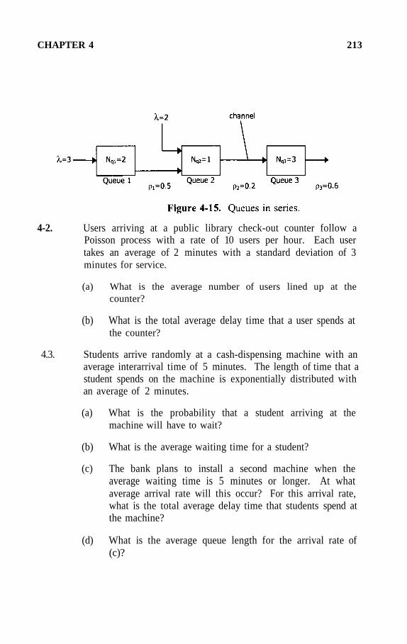
CHAPTER 4 213

4-2. Users arriving at a public library check-out counter follow aPoisson process with a rate of 10 users per hour. Each usertakes an average of 2 minutes with a standard deviation of 3minutes for service.

(a) What is the average number of users lined up at thecounter?

(b) What is the total average delay time that a user spends atthe counter?

4.3. Students arrive randomly at a cash-dispensing machine with anaverage interarrival time of 5 minutes. The length of time that astudent spends on the machine is exponentially distributed withan average of 2 minutes.

(a) What is the probability that a student arriving at themachine will have to wait?

(b) What is the average waiting time for a student?

(c) The bank plans to install a second machine when theaverage waiting time is 5 minutes or longer. At whataverage arrival rate will this occur? For this arrival rate,what is the total average delay time that students spend atthe machine?

(d) What is the average queue length for the arrival rate of(c)?

214 CHAPTER 4

4-4. A concentrator consists of n input lines and a buffer for storingmessages which are transmitted onto an output line with acapacity of 2400 bps. Messages arrive at an input line at anaverage rate of 0.1 messages per second and have anexponential distribution with an average length of 200 bits.

(a) If the maximum possible total average delay at theconcentrator is 1 second, how many input lines can theconcentrator handle?

(b) If what is the average number of messages storedin the buffer?

(c) What is the average waiting time in the buffer?

(d) What is the output line utilization?

4-5. A number of terminals are connected to a concentrator, wheremessages are stored in a buffer and then transmitted in order ofarrival to a computer over a 2400 bps synchronous line. Allmessages from the terminals are exactly 28 bytes long, witheach byte having 8 bits, whereas output messages from theconcentrator are 30 bytes long (the data of 28 bytes plus 2 bytesfor the terminal number). Messages randomly generated at eachterminal follow a Poisson process with an average rate of twomessages per minute.

(a) What is the maximum number of terminals that can beconnected to the concentrator for a stable operation?

(b) What is the total average delay time at the concentrator ifthe number of terminals is 100?

4-6. Measurements are made for a node of a computercommunications network with the following results:

Average number of packets stored in the buffer = 0.1 packets

Average packet length = 500 bits

The output channel has a capacity of

CHAPTER 4 215

(a) If all of the packets are 500 bits long, what is the packetarrival rate?

(b) What is the average transfer delay at the node?

4-7. The capacity of a node in a computer network is 9600 bps.Packets arrive randomly at the node and are all 52 bits long.Under equilibrium conditions, it is found that an average of 4packets are in the system (in the buffer and the output line).

(a) What is the average input rate of this node?

(b) What is the total average delay time through the system?

(c) What is the average number of packets in the buffer?

(d) What is the average waiting time in the buffer?

(e) What is the channel utilization?

4-8. Consider a single-server queueing system, where messagesarrive according to a Poisson process with a rate ofmessages/second. Suppose that the system is idle atFind the probability that the second arriving message will nothave to wait, and also find the average waiting time of thissecond message W for the following two cases: (a) The servicetime X is exponentially distributed with a mean of seconds,and (b)

4-9. Suppose calls arrive at a central office according to a Poissonprocess with a rate of calls per second. Let N be the numberof calls that arrive during a time interval of length T seconds,where T is a nonnegative random variable which is independentof the arrival process, and has the distribution function

mean and variance

Calculate (a) the first moment of N, (b) the second moment ofN, and (c) the variance Var [N].

4-10. Telephone calls arriving at a switchboard follow a Poissonprocess with a rate of 12 calls per minute. (a) What is theprobability that the time interval between the next two calls will

216 CHAPTER 4

be less that 7.5 seconds? (b) More than 10 seconds?

4-11. Consider the birth and death process with the birth and deathrates, and respectively,

and

which corresponds to an Erlang loss system with a single server.(a) Write the differential-difference equations for

and (b) Solve these equationsin terms of and

4-12. Measurements are made in the steady state for a station bufferof a local computer network with channel capacity

The following results are obtained:

Average number of packets stored in the system = 0.1 packets

Average packet waiting time in the buffer = 0.01 milli-seconds

Average packet length = 100 bits and standard deviation = 100bits.

(a) What is the average packet arrival rate?

(b) What is the offered traffic?

4-13. The capacity of the output line of a node in a computer networkis 10 K bps. Under steady-state conditions, it is known that anaverage of 10 messages are stored in the buffer of the node.The average message length is 100 bits and the arrival processis Poisson with an average message arrival rate of 20 messagesper second.

(a) What is the variance of the message length?

(b) What is the average total time delay through the node?

CHAPTER 4 217

(c) What is the average number of messages in the system?

4-14. The link connected to a node in a given network has a bit rateof Measurements in the steady state are obtained asfollows:

Average packet length = 100 bits;

Average number of packets in the buffer = 1.5 packets.

(a) What is the traffic intensity?

(b) What is the total average delay time T at the node?

4-15. Consider a queueing system modeled by a birth and deathprocess with the following birth and death rates:

and

where

(a) Determine the equilibrium probability distribution interms of and k, where and N is thenumber of people in the system;

(b) Find the average number of people in the system.

4-16. A concentrator has m input lines and one output line which hasa capacity of 1200 bps. Each input line has a message arrivalrate of 0.1 messages/second. The message lengths are identicaland exponentially distributed with a mean of 240 bits permessage. Suppose the concentrator can be modeled as anM/M/1 queue.

(a) If the total average concentrator delay is less than or equalto 1 second, how many input lines can the concentrator

Average input rate = 103 packets/sec.;

218 CHAPTER 4

handle?

Let the number of input lines be 30.

(b) What is the average number of messages stored in thebuffer?

(c) What is the average waiting time?

(d) What is the offered load?

4-17. Consider an M/M/1 queue in discrete time, where the time axisis divided into subintervals of 1 second in length. We assumethat events can occur only at the ends of these discrete timesubintervals. The probability of a single arrival is and theprobability of no arrival at that discrete time epoch isSimilarly, if the server is busy at an epoch, then the probabilitythat the service will be completed at the next epoch is andthe probability that it will not finish at the next epoch is

(a) Find the probability that the interarrival time X equals kseconds and the probability that the interdeparture time Yequals k seconds.

(b) Let where N is the number of customersat a discrete time epoch when the system is inequilibrium. Write down the equilibrium equations thatgovern the behavior of and solve them.

4-18. Suppose an M/M/1 queue is operated at an offered load of 0.7erlangs.

(a) What is the average number of customers in the queue?

(b) What is the average waiting time if the average time thata customer spends in the system is 10 seconds?

4-19. Students arrive at a Xerox machine in a Poisson pattern with arate of 10 students per hour. The length of Xeroxing time isexponentially distributed with a mean of 4 minutes.

(a) What is the probability that a student arriving at themachine will have to wait?

CHAPTER 4 219

(b) What is the average waiting time?

(c) What is the average number of students (waiting andbeing served) at the machine?

4-20. Consider a birth and death process with the following birth anddeath rates, respectively,

and

Find

(a) the steady-state probability distribution

(b) the average arrival rate; and

(c) the offered load and the carried load.

4-21. A concentrator with a 1200 bps output line is connected to acomputer. Messages from the input terminals of theconcentrator are all 30 bytes long. Each terminal generatesmessages randomly with a rate of 3 messages/minute.

(a) What is the maximum number of terminals that can beconnected to the concentrator?

(b) If the number of terminals is 80, what is the averagemessage waiting time?

4-22. Consider an M/M/1 queue with the arrival rate of customersper second and service rate of customers per second. Acustomer in the queue will leave without service withprobability in any time interval of length

220 CHAPTER 4

(a) Draw the state-transition-rate diagram.

(b) Express in terms of by equating the flow rate intoa vertical plane separating state k – 1 and state k to theflow rate out of this plane.

(c) Solve for the for

4-23. Consider a cyclic queue in which M customers circulate aroundand pass through two queues as shown below:

Both servers are exponential with rates and respectively.

Let pk = P {k customers in queue 1 and M – k in queue 2}

(a) Draw the state-transition-rate diagram.

(b) Write the relationship between the flow rates into and outof the states.

(c) Find

4-24. Consider a single-server queue (M/M/1) in which there is amaximum possible total of n customers (including the customerin service). Any further arriving customers will be refused andwill depart immediately without service. The arrival rate iscustomers per second and the service rate is customers persecond.

CHAPTER 4 221

(a) Find the equilibrium probability

(b) Find the average number of customers in the system.

(c) Calculate the average arrival rate and the average timethat a customer spends in the system.

4-25. Calculate the interdeparture time distribution function, D(t), foran M /G/1 queue.

(a) Find the Laplace-Stieltjes transform of D(t)conditioned firstly on a non-empty queue left behind, andsecondly on an empty queue left behind by a departingcustomer. Combine these results to obtain the Laplacetransform of the interdeparture time density, and fromthis, determine the probability density function.

(b) For an exponential service time

Find the density function d(t) and the distributionfunction D(t).

(c) For a constant service time

Find the density function d(t) and the distributionfunction D(t).

4-26. Consider an E2/M/1 queue for which the interarrival times ofcustomers have the Erlangian distribution

222 CHAPTER 4

of order r, For E2, we have

Calculate the probability in (4-74).

4-27. Calculate (a) the waiting-time distribution function in theGI/M/1 queue for a first-come, first-served queue discipline,and (b) the mean waiting time.

4-28. Consider a single-server queue with an exponential server ofrate and hyperexponential interarrival time distribution

where Suppose that andCalculate (a) in (4-74), (b) and (c) the mean

waiting time W.

4-29. A communication line capable of transmitting at a rate of 96Kbps will be used to connect 10 stations, each generatingPoisson traffic at a rate of 5 packets per second. Packet lengthsare identical and exponentially distributed with a mean of 1000bits. For each station, calculate (a) the average number ofpackets in the queue, (b) the average number of packets in thesystem, and (c) the average transfer delay per packet when theline is allocated to the stations by using (i) 10 equal-capacitytime-division multiplexed channels, and (ii) statisticalmultiplexing.

4-30. A data-storage device consists of a rotating disk which storesblocks of data in sectors. A sensor called a head is locatedclose to the rotating surface and can read or write data blocks atsome predetermined sector. All blocks begin on a sectorboundary. Suppose that read/write requests arrive at the headqueue according to a Poisson process with an average rate ofrequests per second. Each of these requests demands a block ofdata of fixed length b sectors beginning at a random sector

CHAPTER 4 223

boundary. Calculate the mean waiting time for a disk access,given that the disk rotates at a rate of r revolutions per secondand has s sectors. Assume that the system can be modeled byan M/G/1 queue.

CHAPTER 5

THE ERLANG LOSS AND DELAY SYSTEMS

5-1. INTRODUCTION

Having studied the birth and death process in detail in the lastchapter, this chapter will investigate several fundamental questionsconcerning the service of incoming calls by a number of lines. Theseincoming calls follow a Poisson process with a constant arrival rate.

The process of service operates in such a way that each incoming calloccupies a free line for a period of time, called the holding time or servicetime. While a line is busy with a call, it is inaccessible to other calls.

If, upon arrival, an incoming call finds all lines busy, the call is saidto be blocked. In problems of telephone system design, there are two waysto handle blocked calls: (a) The blocked call is simply refused and is lostas though it had not occurred at all. This type of system is called a losssystem; (b) A blocked call remains in the system and waits for a free line.This type of system is known as a delay system. These two types ofsystems differ from each other not only in details regarding solutions tobasic problems, but also in their structures. The important fact is that thegrade of service in these two systems are completely different. For a losssystem, the grade of service is the probability of blocking. On the otherhand, for a delay system, the grade of service is the probability of waiting,and the central problem involves the investigation of the waiting time as arandom variable.

In this chapter, we shall investigate both the Erlang loss and delaysystems. We shall also present some important features of the Erlangsystems and examine the two systems in separate sections.

Full Accessibility. A system with a collection of lines is said to be afully-accessible system if all of the lines are equally accessible to allincoming calls. For example, the trunk lines for interoffice calls are fully-accessible lines.

Characteristics of the Erlang Systems. The Erlang systems may bedefined by the following specifications:

CHAPTER 5 225

1. The arrival process of calls is assumed to be Poisson with a rate ofcalls per hour.

2. The holding times are assumed to be mutually independent andidentically distributed random variables following an exponentialdistribution with a mean of seconds.

3. The system has s lines serving the calls.

4. Calls are served in order of arrival.

Let the state of the system at time t be defined as the number of callsin the system at t, and consider the probabilities for the state transition in asmall time interval It follows from the above specifications thatthe probability of transition from state k to state k + 1 in is

for the probability of transition from state k tostate k – 1 in is since there are k busy lines andeach line becomes free in the time interval with a probability

For this transition probability becomesfor delay systems. By comparison of these state transition probabilities andthose of the birth and death process, we see that the behaviour of theErlang system in state k can be described by the birth and death processwith the birth rate and death rate The Erlang systems can bemodeled as an M/M/s queue.

5-2. THE ERLANG LOSS SYSTEM

Consider the Erlang loss system with s fully-accessible lines andexponential holding times. In queueing theory, servers associated withexponential service time distribution are often called exponential servers.A queueing model for the Erlang loss system is shown in Figure 5-1,where the waiting capacity is zero, i.e. no waiting is allowed.

The Erlang loss system can be modeled by the birth and deathprocess with the birth and death rates as follows:

and

226 CHAPTER 5

Under equilibrium conditions, the state probability distributioncan be obtained from (4-24) as follows:

Substitution of the birth and death rates (5-1) and (5-2) into (4-24) gives

By defining the offered traffic

(5-3) can be written as

CHAPTER 5 227

The probability is determined by the normalization condition

Therefore,

Finally, combination of (5-4) and (5-5) yields

This probability distribution is called the truncated Poisson distribution orErlang’s loss distribution.

In particular, when the probability of loss is given by

In the Unites States, (5-7) is called the Erlang loss formula or the Erlang Bformula and in Europe, it is called Erlang’s first formula and is denoted by

It is important to point out that the truncated Poisson distribution (5-6) is valid for any holding time distribution with a finite mean of eventhough the Markov property of the exponential holding time distributionwas used explicitly in the derivation. This remarkable fact was conjecturedby Erlang himself in 1917, and proven by Sevastyanov in 1957. Valuesfor B(s,a) obtained from (5-7) have been plotted against the offered traffica in erlangs for different values of the number s of lines. Two typical

228 CHAPTER 5

groups of Erlang B curves are given in Figures 5-2 and 5-3.

The Erlang B formula gives the time congestion of the system andrelates the probability of blocking to the offered traffic and the number oftrunk lines. In design problems, it is usually necessary to find the numberof trunk lines needed for a given offered traffic and a specified grade ofservice.

The ratio is called the offered load or offered traffic. It is adimensionless quantity that is numerically equal to the average number ofincoming calls that occur during an average holding time. Theinternational unit for the offered traffic is the erlang. One erlang representsthe amount of traffic that occupies one piece of traffic-sensitive equipment(a circuit or a trunk) busy for one hour. Thus one erlang is equal to one

CHAPTER 5 229

call-hour per hour and it is a dimensionless unit.

More generally, the offered load generated by a Poisson input processwith a rate of calls per hour may be defined as the average number ofincoming calls per holding time; that is,

where is the average number of incoming calls in a fixed time intervalof t hours and H(t) is the holding time distribution and is the averageholding time.

230 CHAPTER 5

The average number of occupied or busy trunks is defined as the carriedload:

For the Erlang loss system, the carried load is given by

Thus, the carried load is the portion of the offered load that is not lostfrom the system.

The carried load per line is known as the trunk occupancy:

The trunk occupancy is a measure of the degree of utilization of a groupof lines and is sometimes called the utilization factor.

Investigation of formulas (5-7), (5-10), and (5-11) indicates that asthe offered load and the number of lines are increased such that theprobability of blocking remains constant, the line occupancy increases. Inother words, large line groups are more efficient than small ones.Unfortunately, the size of a line group is limited by hardware complexity,and high-occupancy line groups are more vulnerable to service degradationduring periods of overload than the smaller line groups with the sameblocking probability but lower occupancy.

To illustrate this point, let us consider a trunk group with an offeredload of 4.5 erlangs and a blocking probability of 0.01. From the Erlang Bcurves in Figure 5-2, we find that 10 trunks are required. If the offeredload is increased to 12 erlangs, then in order to keep the blocking

CHAPTER 5 231

probability at 0.01, 20 trunks are needed. Since

we calculate the trunk occupancies as follows: Using (5-10) and (5-11),we get

and

Thus, the group of 20 trunks is more efficient than the group of 10 trunks.

For a trunk group of fixed size, occupancy increases with increasingload, thereby increasing trunk group efficiency; unfortunately, theprobability of blocking also increases with increasing load. Hence,efficient use of equipment must be balanced against the provision ofacceptable grade of service.

The above discussion does not take into account the effect of trafficoverload. In designing a telephone system, it is necessary to ensure thatthe system will operate satisfactorily under a moderate overload condition.Figure 5-4 shows the effect of overload on the blocking probability forvarious sized groups of trunk lines. For each sized group, the originaltraffic carried is assumed to be at a 0.01 grade of service. From Figure 5-4, we see that a 20% overload on a 10-line group causes the grade ofservice to worsen to 0.024. The same overload on a 20-line group causesthe grade of service to worsen to 0.035. The larger, more efficient groupis therefore more sensitive to overload. Above a certain traffic level, thenumber of lines needed is determined by the required overload performancerather than the basic offered traffic. For example, a typical designrequirement might be that a normal grade of service of 0.01 shouldincrease to no more than 0.02 for a 10% overload. In this case, the groupsize should be no more than 20 lines.

232 CHAPTER 5

In telephone switching networks, the term availability or accessibilityis used to define the capacity or number of outlets of a switch to access agiven route. For example, in an m × n switch, the availability is n. Theavailability is usually designated by the letter k.

The term full availability is applied when any inlet of a switch hasaccess to all of the trunks in a given route. In practice, it is moreeconomical to use smaller switches with restricted availability (restrictedblocking). However, it is also desirable to obtain good utilization. Thisimplies the use of a large number of crosspoints in a switching network.Thus, there is a compromise between the utilization and the overload

CHAPTER 5 233

performance.

Example 5-1. Consider the telephone trunking problem. Atelephone exchange A is to serve 10,000 subscribers in a nearby exchangeB as shown in Figure 5-5. Suppose that during the busy hour, thesubscribers generate a Poisson traffic with a rate of 10 calls per minute,which requires trunk lines to exchange B for an average holding time of 3minutes per call. Determine the number of trunk lines needed for a gradeof service of 0.01. Also calculate the lost traffic and the utilization factor.

Solution. Since there are 10,000 telephone subscribers, the inputtraffic may be assumed to be Poisson. The average calling rate iscalls/hour, and the average holding time is seconds. The offeredtraffic is erlangs.

Using the Erlang B curves in Figure 5-3, we find that for a grade ofservice of 0.01, the number of trunk lines needed is 41. Since the carriedload is given by

234 CHAPTER 5

the lost traffic is equal to

and the utilization factor is given by

Example 5-2. Consider a switch whose control causes it to searchsequentially for a free line. The control always starts searching in thesame order and from the same starting position. Suppose that the totaltraffic offered to the lines is a erlangs. Calculate the traffic carried by thenth line in the system under the condition that the input is Poisson andblocked calls will be cleared.

Solution. This system may be considered as an Erlang loss systemwith sequential hunting. The traffic lost to the (n – 1)th line isaB(n – 1, a), and the traffic lost to the nth line is aB(n ,a). However,the traffic lost to the (n – 1)th line is the traffic offered to the nth line.Thus, the traffic carried by the nth line is the difference between theoffered traffic and the lost traffic to the nth line,

where B(n, a) is given by (5-7) with

In particular, if a traffic of 5 erlangs is offered to a number of lines, thetraffic carried by the first line is

CHAPTER 5 235

The traffic carried by the second line is

and the traffic carried by the third line is

We see that the traffic carried by latter choice lines are getting smaller, buttheir presence is essential to provide the required grade of service.

Example 5-3. Four groups of terminals are to be multiplexed andconnected to a computer, as shown in Figure 5-6. In Figure 5-6(a), the

236 CHAPTER 5

traffic from each group uses a separate group of circuits. In Figure 5-6(b),all terminals are combined into one group using only one common groupof circuits. Determine the total number of circuits required in both caseswith a specified grade of service of 0.01. Assume that each terminal offersa traffic of 0.1 erlangs.

Solution. The offered traffic from each group of terminals in Figure5-6(a) is

CHAPTER 5 237

Since the average number of active terminals is much smaller than thenumber of terminals in a group, we may assume that the input traffic isapproximately Poisson.

Using the Erlang B curves for a grade of service of 0.01 at a loadingof 2 erlangs, 7 circuits are required for each group. Thus, theconfiguration of Figure 5-6(a) requires a total of 28 circuits.

The total offered traffic to the concentrator of Figure 5-6(b) is

From the Erlang B curves, we find that the required number of circuits fora grade of service of 0.01 at a load of 8 erlangs is 15.

This example demonstrates that combining several small trafficgroups into one large traffic group can provide significant savings in thetotal number of circuits required.

5-3. THE ERLANG DELAY SYSTEM

Consider a telephone exchange in which incoming calls follow aPoisson input process with calling rate The calls are served by s fully-accessible lines. The holding times are assumed to be mutuallyindependent, identical, and exponentially distributed with an averageholding time of

An incoming call must wait for service when it finds all s lines occupied.The probability of finding all of the lines occupied is called the probabilityof waiting. Waiting calls are served in order of arrival. A systemsatisfying these conditions is called an Erlang delay system.

The objective in the investigation of delay systems is not onlyconcerned with the frequency of delay, but also the distribution function ofthe waiting time. Thus, the nature of the waiting time W as a randomvariable plays a decisive role in the study of delay systems.

238 CHAPTER 5

Suppose that the system is in state k at an arbitrary moment; that is,there are k calls (in service and waiting) in the system. If k linesare occupied and no calls are waiting. If all s lines are occupiedand there are k – s calls waiting. A queueing model for the Erlang delaysystem is shown in Figure 5-7, which is an M/M/s queue.

Note that if the Erlang delay system is operated in exactly thesame way as the Erlang loss system, since for there are neither lostcalls nor waiting calls. However, when the operation is completelydifferent. Since the transition is now possible from state s into state s + 1which is impossible for a loss system, by taking the waiting calls intoconsideration, we can model the Erlang delay system by the birth anddeath process with the following birth and death rates, respectively,

and

Under equilibrium conditions, the state probability distributioncan be obtained by substituting these birth and death rates into (4-24) toyield

CHAPTER 5 239

Using the normalization condition

we find

where the condition has been assumed. Furthermore, theprobability of waiting (the probability of finding all lines occupied) is equalto

240 CHAPTER 5

where W is a random variable denoting the waiting time and is theprobability that the system is in state k just prior to an arrival. If the inputprocess is a Poisson process, then (see (5-30)). In the UnitedStates, (5-18) is called the Erlang delay formula or the Erlang C formula.In Europe, it is known as Erlang’s second formula and is denoted by

Two typical groups of Erlang C curves are given in Figures 5-8and 5-9.

CHAPTER 5 241

Unlike the Erlang loss system, the state probability distribution of theErlang delay system constitutes a proper distribution only when the offeredtraffic is less than the number of lines in the system.

From the definition of the carried load, we have

242 CHAPTER 5

Using (5-16) and (5-18), the last term on the right-hand side can be writtenas

Consequently, we obtain

This result shows that for an Erlang delay system, the carried and offeredloads are always equal. This is intuitively clear because in a delay system,all calls are served and there is no loss.

The Average Number of Calls in the Erlang Delay System andthe Mean Waiting Time. By definition, the average number of calls in adelay system is given by the general expression

Using (5-16), for the Erlang delay system, we have

CHAPTER 5 243

The first summation on the right-hand side is equal to

and the second summation may be written as

since the quantity in the brackets on the left-hand side is simply equal to

where

Consequently, we find the average number of calls in the system:

Note that the first term on the right-hand side is the average queue lengthor the average number of calls waiting in the queue, and the second

term is the average number of busy lines. Now, using Little’s formula, we

244 CHAPTER 5

find the mean waiting time:

Example 5-4. Consider the telephone trunking problem studied inExample 5-1, except that if, on arrival, a call finds all trunk lines busy, thiscall will wait until a line is freed. In this case, the grade of service is theprobability of waiting. Determine the number of lines needed for a gradeof service of 0.01, the average number of calls in the system, and the meanwaiting time.

Solution. From example 5-1, we have an offered traffic of 30erlangs. Using the Erlang C curves in Figure 5-9, we find that for aprobability of waiting of 0.01, the number of lines needed is 44.

In this example, we see that in order to avoid the loss of 0.3 erlangsas found in Example 5-1, it is necessary to add 3 more lines to the systemso that a probability of waiting of 0.01 is maintained.

Since the average number of calls in the

system is then given by

The mean waiting time is given by (5-20):

CHAPTER 5 245

5-4. THE COMBINED DELAY AND LOSS SYSTEM

In the Erlang loss system, no waiting is allowed, while in the Erlangdelay system, the waiting capacity is assumed to be infinite and hence noloss can occur. In practice, the waiting capacity is always finite.Investigation of this more realistic system is possible by means of thenotion of combined delay and loss system. The combined delay and losssystem can also be modeled by the birth and death process.

Consider the Erlang delay system of the last section with a finitewaiting capacity of n – s. Now we have, by taking into consideration thefact that the combined delay and loss system can have only n + 1 possiblestates, the modified birth and death rates

and

Substituting and into (4-24), we obtain

where

246 CHAPTER 5

The probability of waiting is given by

The probability of loss is equal to

Note that when (5-26) reduces to the Erlang B formula (5-7).Therefore,

Similarly, when the probability of waiting in (5-25) becomes theErlang delay formula (5-18):

Furthermore, the probability in (5-24) reduces to the in (5-17).Therefore, the Erlang loss system and the Erlang delay system may be

CHAPTER 5 247

regarded as special cases of the combined delay and loss system.

5-5. THE OUTSIDE OBSERVER’S DISTRIBUTION AND THEARRIVING CUSTOMER’S DISTRIBUTION

In the investigation of the Erlang systems, the state probabilitydistribution was derived from equations which relate the proportionsof time that the system spends in various states to each other. Therefore,for systems in equilibrium, may be interpreted either as the proportionof time that the system spends in state k or as the probability that thesystem is in state k at an arbitrary moment. The distribution of timethat the system spends in each state is called the outside observer’sdistribution. Now let denote the state probability distribution that anarriving call would encounter; that is, the state probability distribution withrespect to only those arrival instants of the call. In queueing theory, thedistribution is called the arriving customer’s distribution. It isimportant to realize that, in general, the outside observer’s distributionand the arriving customer’s distribution are different. However, forsystems with Poisson input, these two distributions are identical. This factis of central importance in the calculation of the waiting time distributionin the Erlang delay system.

Consider a record of the states of a telephone exchange shown inFigure 5-10. Suppose that n calls occur in the observation interval (0, t).The proportion of time that the system spends in state k is given by

where is the total time that the system spends in state k during

the interval (0,t) and where is the number of subintervals during whichthe system is in state k. In a telephone system with s lines, the quantity

is known as the time congestion. The observation interval

is usually taken as the sum of the BH (busy-hour) traffic on the 10 busiestdays of the year,

248 CHAPTER 5

Another important quantity of practical significance is the proportionof calls that, on arrival, find the system in state k:

where is the total number of calls that, upon arrival, find the system in

state k during the observation interval (0, t). The quantity

is known as the call congestion. In general, time congestion and callcongestion are not equal; they become equal when the input process isPoisson.

To investigate the relationship between the outside observer’sdistribution and the arriving customer’s distribution we letN(t) denote the number of calls in the system at time t, and letA (t, ) be the event that a call arrives in the time interval ( t , ).Let

CHAPTER 5 249

= the probability that the outside observer finds

the system in state j at time t,

and

= the probability that the system is in state j at time t

just prior to an arrival epoch.

By definition, we write

Using Bayes’ rule of probability theory, we can write

It follows that

If the arrival process described by A(t, ) is a birth and deathprocess, then

250 CHAPTER 5

and

This result shows that for a birth and death process,

If the arrival process is a Poisson process, then

for all j

In this case, we obtain from (5-29)

As or when the system is in equilibrium, we obtain

and hence,

CHAPTER 5 251

This result implies that for a queueing system with a Poisson input, thearriving customer’s distribution and the outside observer’s distribution areequal, and relation (5-30) is called Poisson Arrivals See Time Averages(PASTA).

5-6. THE WAITING TIME DISTRIBUTION FUNCTION FOR THEERLANG DELAY SYSTEM WITH SERVICE IN ORDER OFARRIVAL

Consider the probability that a test call entering thesystem at a random moment has a waiting time greater than t. Let

be the conditional probability of the event on theassumption that, on arrival, the test call finds the system in state k. Usingthe formula of total probability, we write

where is the probability that the system is in state k just prior to thearrival epoch of the test call. Since for andwe have

Since the input process is Poisson, then where is given by (5-16). It remains to determine the conditional probabilities forall

Note that if there must be k – s calls waiting for service inthe queue. If the queue discipline is first-come, first-served or service inorder of arrival, then a call finding k – s calls waiting in the queue willobtain service after the (k – s + l)th freeing of line. Thus, the conditionalprobability is equal to the probability that during the timeinterval t after the arrival of the test call, there will be at most k – s

252 CHAPTER 5

freeings of line. It follows that

where denotes the probability of exactly r freeings of line in the timeinterval t, which remains to be determined. Since the holding time hasthe exponential distribution

the probability that no freeings occur during the time interval t from thearrival moment of the test call is equal to

This implies that the number of freeings of line during the time interval tis a Poisson process with freeing rate Thus, the interfreeing timefollows an exponential distribution with mean Therefore, theprobability of exactly r freeings during the time interval t is given by aPoisson process with rate

This result indicates that when all s lines are busy, the process of freeingbusy lines follows a Poisson process with rate

Substituting into (5-32) yields

Since the input process is Poisson, for we obtain from (5-16) and(5-30):

CHAPTER 5 253

Substituting and into (5-31) gives

We see that, under the stated conditions, the waiting time has anexponential distribution with a parameter of Note that, asexpected

In addition, the waiting time distribution in (5-34) is valid for the Erlang

254 CHAPTER 5

delay system with service in order of arrival discipline and exponentialservice time distribution.

The mean waiting time is given by

which is the same as (5-20). The second moment of the waiting time isgiven by

Thus, the variance of the waiting time is given by

CHAPTER 5 255

Example 5-5. Consider an airline seat reservation office in whichthere are five assistants. Each has his own terminal connected to an on-line booking system. Assume that arriving customers follow a Poissonprocess with a rate of 40 customers during the busy hour of the day, andthat the five assistants give similar exponential services with an average of5 minutes. (a) How long a customer can expect to wait in a queue? (b)How long is the queue expected to be? (c) What is the effect of a 10%increase in the customer arrival rate on the mean waiting time and themean queue length? (d) What is the variance of the new waiting time?

Solution. (a) The mean arrival rate The

mean service time

The offered load is

Then the utilization factor Using the Erlang

delay curves, we find

Hence,

(b) Using Little’s formula, the mean queue length is given by

(c) For a 10% increase in the new input rate becomes

256 CHAPTER 5

and the corresponding utilization factor now becomes

Now the new offered load is

Then, the new mean waiting time is

which increases by (1.63 - 0.96)/0.96 = 70%, and the new mean queuelength is

which increases by (1.19 - 0.64)/0.64 = 86%.

(d) Using (5-36), we find

5-7. THE WAITING TIME DISTRIBUTION FOR THE COMBINEDDELAY AND LOSS SYSTEM WITH SERVICE IN ORDER OFARRIVAL

If the Erlang delay system has a finite n – s waiting capacity,arriving calls which find the system in state n will be lost. In this case,the system becomes a combined delay and loss system. Waiting ispossible only when If or and then

CHAPTER 5 257

Thus, using the formula of total probability, the waitingtime distribution with service in order of arrival can be writtenas

Using (5-23) and the conditional probability in (5-33), we find

where

258 CHAPTER 5

and is given by (5-24).

5-8. OVERFLOW TRAFFIC

For the Erlang loss system, it was assumed that blocked calls (thosecalls which find all circuits busy) would be cleared from the system andwould not return. In practical applications, blocked calls are routed toanother similar group of circuits. For example, calls in an alternate routingnetwork can take alternate routes when all of the circuits in the directroutes are busy. The traffic overflowed from the primary or direct routes(first-choice routes) is called the overflow traffic, and will be handled by analternate trunk group.

To study the overflow traffic, we shall determine the mean andvariance of the overflow distribution. First, we shall consider a queueingsystem composed of an s-server primary group and an infinite-serveroverflow group. The queueing model is shown in Figure 5-11.

CHAPTER 5 259

We assume that customers request service first from the s-serverprimary group, and that customers who find all servers busy in the primarygroup, overflow to and are handled by the infinite-server overflow group.The input traffic is Poisson with rate and the service times areindependent, identical and exponentially distributed with mean

Let M and N denote the number of customers that are being servedsimultaneously in the primary and overflow groups, respectively.Furthermore, we let

be the statistical-equilibrium state probability of the system.

Consider the possible changes of state during a small time interval(t, ) and display the possible transitions from state (j, k) to itsneighboring states by using a two-dimensional state-transition-rate diagramas shown in Figures 5-12(a) and (b).

260 CHAPTER 5

Using Figures 5-12(a) and (b), we write the following probabilityflow rates. For we have



For j = s, we write

CHAPTER 5 261



Equating the flow rates into and out of the corresponding states yield,respectively,

and

or

and

where

262 CHAPTER 5

This set of equations (5-40) and (5-41) is subject to the normalizationcondition

To solve the equations (5-40), (5-41), and (5-42), we consider theaugmented system of equations obtained from (5-40) by extending s toinfinity:

where

We shall solve the set of equations in (5-43) in such a way that

Define the two-dimensional probability-generating function

Multiplying (5-43) by and summing for j and k from 0 to yieldsthe partial differential equation

whose general solution is

CHAPTER 5 263

Using this generating function, R.B. Cooper (see reference [1], p.139), obtained the following formulas for the mean and thevariance Var[N] = v:

and

where is the offered load in erlangs and B (s, a) is the probabilityof loss given by the Erlang loss formula (5-7). Expressions (5-49) and (5-50) are called the Wilkinson formulas.

5-9. THE EQUIVALENT RANDOM METHOD

A telephone network where calls to a destination can take alternateroutes is called an alternate routing network. A simple alternate routingnetwork for direct distance dialing calls is shown in Figure 5-13. In thisfigure, switching nodes are denoted by lettered circles; first-choice routesand intermediate routes are represented by dashed lines which are high-usage routes, and final routes are represented by solid lines. The directionof overflow traffic is shown by a curved arrow.

The traffic originating from node A and destined for node D isassumed to be Poisson with a rate of calls per second. The holdingtimes of calls are independent, identical and exponentially distributedrandom variables with a mean of seconds. Thus, the primary trunkgroup of the first choice routes operates like an Erlang loss system. Thetraffic which overflows the primary trunk group will be handled by theintermediate routes. Similarly, the traffic which overflows the intermediatetrunk group will be handled by the final trunk group. Thus, both theintermediate trunk group and the final trunk group may carry the first-attempt Poisson traffic and act as alternate routes. The overflow traffic isnot Poisson and will be approximated by its mean and variance.

To investigate the blocking in the alternate routing network, we shallcalculate the proportion of calls which overflow the intermediate overflowgroup, given that these calls overflow the first-choice primary group.

264 CHAPTER 5

We shall describe an approximation technique, called the equivalentrandom method, which was developed by R.I. Wilkinson. We shall alsodetermine the number of servers and the particular server arrangementssuch that a sufficient number of servers will ensure that a prespecifiedprobability of loss (overflow from both primary and overflow servers) isnot exceeded.

Consider the alternate routing network whose model is shown inFigure 5-14. The network has n primary groups; each primary groupconsists of trunks and receives a direct Poisson offered load oferlangs. All traffic overflowing the n primary groups is handled by acommon overflow group of c trunks. The holding times on all groups areassumed to be independent, identical and exponentially distributed.

For the purpose of analysis, we represent approximately the load(traffic) that overflows the kth primary group by two parameters, the mean

and variance which are calculated by (5-49) and (5-50),respectively:

CHAPTER 5 265

This implies that the load overflowing a primary group is representedapproximately by the mean and variance of the overflow distribution thatwould result if the overflow traffic were handled by an infinite-serveroverflow group.

We shall calculate the probability that a call arriving at the kthprimary group and finding all sk lines busy will also find all c lines busy inthe overflow group. We denote by a the mean value of the load thatoverflows the s-server primary group.

We replace the n primary groups and their respective equivalentPoisson offered loads with a single equivalent random primary group and asingle equivalent random load so that we have the equivalent randommodel for Figure 5-14, as shown in Figure 5-15.

Since the n primary groups in Figure 5-14 are mutually independent,we choose both the number of s servers in the equivalent random primarygroup and the equivalent random (offered) load a in Figure 5-15 such thatthe total overflow load offered to the c-server overflow group is the sameas that in Figure 5-14. Thus, we let

266 CHAPTER 5

With the values of and v calculated by (5-53) and (5-54),respectively, we describe Rapp’s approximate formulas for determining thevalues of a and s from (5-49) and (5-50) as follows. In terms of thepeakedness factor

and

CHAPTER 5 267

These estimates of a and s are generally on the high side of the exactvalues. By rounding s down to its integral part we obtain thecorresponding value of a by solving (5-56):

It follows that the load overflowing the c-server overflow group isapproximately equal to

In the equivalent random system of Figure 5-15, the proportion of callsoverflowing both the equivalent random primary group and the overflowgroup is given by

which is the probability of blocking on the overflow group suffered by theoverflow traffic from the n primary groups. Similarly, the proportion oftraffic that is blocked on both the primary and overflow groups isapproximated by

The equivalent random method has proven to be useful in teletrafficengineering. Given a blocking probability, the values of a and s, we candetermine the number of trunks c in an alternate routing network using theErlang B curves.

The equivalent random method is to replace the network in Figure 5-14 with the network in Figure 5-15, where the values of a and s arechosen approximately such that the mean α and variance v of the overflowtraffic remain the same in both networks.

268 CHAPTER 5

Example 5-6. Consider the outgoing trunk groups on a privateswitching system. Suppose that blocked calls on these outgoing trunkgroups are neither queued nor rerouted so that the callers merely hang upand try again. Trunk groups operated in this way are known as stand-alone trunk groups. They carry first-route traffic only. Thus, the offeredtraffic to the stand-alone trunk groups is assumed to be random or Poisson.Figure 5-16 shows the traffic flow on a stand-alone trunk group.

Assume that the busy-hour offered traffic to the outgoing trunk groupis 5 erlangs.

(a) What is the apparent offered load if the grade of service or blockingfactor is 0.04?

(b) How many stand-alone trunks should be installed?

Solution. From Figure 5-16, we write

Thus,

CHAPTER 5 269

where

is called the apparent offered load adjustment factor. Furthermore, we alsowrite

Hence, using (5-61) and solving for a gives

where

is known as the offered-load adjustment factor.

(a) Since a = 5 erlangs and using (5-61) and (5-62), we get

(b) Using the Erlang loss curves in Figure 5-2, we find that the numberof required stand-alone trunks is equal to 9.

Example 5-7. Poisson traffic of a erlangs is offered to a primarygroup (or routes) of s trunks. Assume that blocked calls are routed to asecondary route.

270 CHAPTER 5

(a) Show that the variance of the carried traffic of the primary route isgiven by

(b) In particular, let a = 15 erlangs and the number of primary trunks be20. Calculate the mean and variance of the carried load. What is thepeakedness factor of the carried load?

(c) Calculate the mean and variance of the overflow traffic that is offeredto the secondary route. What is the peakedness factor of theoverflow traffic?

Solution. (a) Using (5-4), (5-9) and (5-10), we write

Writing in the form

and factoring out ( ) yield the required expression (5-65).

(b) Using (5-10), (5-65) and the Erlang loss curves in Figure 5-3, we get

CHAPTER 5 271

The peakedness factor of the carried load is given by

Note that " Thus, the carried traffic is smooth.

(c) Using (5-49) and (5-50), we obtain

The peakedness factor of the overflow traffic is given by

Since the overflow traffic has a peakedness factor greater than unity, it isrough.

Example 5-8. Consider the alternate routing network shown inFigure 5-17. Suppose that the mean and variance of the overflow trafficare 3.88 erlangs and 6.29, respectively. Determine the equivalent randomtraffic and the number of trunks in the primary route so that the blocking

272 CHAPTER 5

probability of both the primary and secondary routes will be 0.01. What isthe lost traffic of the network?

Solution. Since erlangs and v = 6.29, the peakednessfactor is

Using Rapp’s approximate formulas (5-55) and (5-56), we get

By rounding s to 6, we obtain from (5-57) the equivalent Poisson (random)traffic

CHAPTER 5 273

Using the Erlang loss curves in Figure 5-2 with the equivalent randomtraffic of 8.9 erlangs and blocking probability of 0.01, we find

since s = 6.

The lost traffic of the network is

Example 5-9. To illustrate the application of the equivalent randommethod, we consider the alternate routing network shown in Figure 5-18,where the offered load and the economic traffic are given as follows:

The economic traffic is known as the economic CCS (or ECCS) in theU.S.A. This is the minimum traffic that the last trunk in a trunk groupshould carry. If the last trunk in a trunk group carries less traffic than theeconomic traffic, it would be cheaper to reroute the last trunk’s traffic to analternate route.

(a) What is the number of trunks in the two direct routes such that thelast trunk in the trunk group will carry a traffic greater than thecorresponding economic traffic?

(b) Calculate the mean and variance of the overflow traffic from thedirect routes.

(c) What is the peakedness factor of the overflow traffic?

(d) Calculate the equivalent random traffic and the number of trunksrequired.

(e) Calculate the number of trunks in the alternate trunk group, given thatthe blocking probability in the final group is 0.01.

274 CHAPTER 5

Solution. (a) For the direct trunk group between nodes A and B, wefind by use of (5-12) and Figure 5-2 that

which is greater than or 0.409 erlangs. Note that(0.130 - 0.086) = 0.3168 erlangs which is less than Thus,

the number of trunks in this trunk group is 9. Similarly, for the directtrunk group between nodes A and C, we have

which is greater than and hence, the number of trunks in this trunkgroup is 12.

CHAPTER 5 275

(b) Using (5-51) and (5-52), we obtain

and

Thus,

(c) The peakedness factor of the overflow traffic is

(d) Using (5-55) and (5-56), we find

By rounding this value of s to 11, we obtain the equivalent randomtraffic using (5-57):

276 CHAPTER 5

and the required number of equivalent trunks is 11.

(e) For a blocking probability of 0.01 and an equivalent random offeredtraffic of 10.7972 erlangs, we find from the Erlang B curves

or

5-10. SUMMARY

The Erlang loss system and the Erlang delay system are investigatedusing the birth and death process as a model. By specifying thecorresponding birth and death rates, the Erlang loss distribution and theErlang loss formula are obtained. The carried load in the Erlang losssystem is then calculated in terms of the offered load and the lossprobability. Similarly, the Erlang delay formula for the calculation ofwaiting probability is derived. In addition, the average number of calls andthe mean waiting time in the Erlang delay system are determined.

It is important to note that the Erlang loss formula or the Erlang Bformula is valid for arbitrary holding time distributions. However, theErlang delay formula or the Erlang C formula is true only when the trunkoccupancy is less than unity so that the system can reach the steady stateor equilibrium conditions. In practical applications, curves for the ErlangB and Erlang C formulas are available and convenient to use.

When calculating the waiting time distribution, the queue disciplinemust be specified. The Erlang delay system assumes service in order ofarrival or FIFO queue discipline. When there are calls waiting for servicein the queue, all servers or trunk lines are busy. This leads to the fact thatunder the condition of all servers being busy, the departing process isPoisson with rate As a result, the calculation of the waiting time

CHAPTER 5 277

distribution is greatly simplified.

For the study of alternate routing networks, the equivalent randommethod is useful when the overflow traffic from the first choice routes isapproximated by its first two moments or the mean and variance. Anexample is given to illustrate the application.

REFERENCES


[2] Khintchine, A.Y., Mathematical Methods in the Theory of Queueing,2nd ed., New York: Hafner, 1969.


[4] Fry, T.C., Probability and Its Engineering Uses, 2nd ed., New York:Van Nostrand, 1965.

[5] Bucher, J.R., Traffic System Design Handbook, Piscataway, N.J.:IEEE, 1992.

[6] Hills, M.T., Telecommunications Switching Principles, Cambridge,Mass., MIT Press, 1979.

[7] Martine, R.R., Basic Traffic Analysis, Englewood Cliffs, N.J.:Prentice Hall, 1994.

[8] Wilkinson, R.I., "Theories for Toll Traffic Engineering in theU.S.A.", Bell System Tech. J., Vol. 35, No. 2, 1956, pp. 421-514.

PROBLEMS

5-1. An average of 150 calls per hour calling rate with an averageduration of five minutes per call is offered to a trunk group.The trunks must provide a 0.005 grade of service.

(a) How many stand-alone trunks are required?

(b) How many trunks are needed to ensure a 0.01 grade ofservice?

278 CHAPTER 5

(c) What is the grade of service for 20 trunks?

5-2. The following measurements were made on an outgoing trunkgroup during the busy hour:

Number of originating calls = 294.

Number of overflow calls = 6.

Number of times that all trunks are busy is 12, with an averageof 8 seconds per period.

(a) What is the time congestion?

(b) What is the call congestion?

5-3. Consider that a connection between the central computer of thehead office of a bank and a data terminal of its branch office isestablished at 1:00 A.M. Assuming that the average calling ratefor connection is 1 call per hour and the connection wasmaintained continuously. If data are transferred at a rate of9600 bits per second, determine the amount of traffic in erlangstransferred over the established connection between 1:00 A.M.and 1:45 A.M.

5-4. A group of 10,000 subscribers originate an average rate of 500calls per hour with a mean holding time of 200 seconds.

(a) What is the offered traffic in CCS?

(b) What is the offered traffic per subscriber in CCS?

(c) How many erlangs of traffic originated by a subscriber?

(d) If the system is operated on a blocked call cleared basiswith a group of 38 trunks, what is the blockingprobability?

(e) What is the carried load per trunk?

CHAPTER 5 279

5-5. Show that

5-6. Show that

5-7. Consider an Erlang delay system with s exponential lines ofmean service time seconds and Poisson input of ratecalls per second. A test call entering the system at findsall s lines busy with n waiting calls. Waiting calls are servedin order of arrival. Service times are assumed to be mutuallyindependent, identical, and exponentially distributed randomvariables.

(a) Find the mean waiting time for the test call in the queue.

(b) Suppose that no new calls arrive at the system afterWhat is the expected length of time from the arrival of thetest call at until the system finishes serving all thecalls?

(c) Let X be the order of completion of serving the test call;that is, if the test call is the kth call to have beencompletely served after Find

(d) What is the probability that the test call has beencompletely served before the call immediately ahead of itin the queue?

5-8. A concentrator consists of a number of input lines, each havingPoisson input traffic with a constant rate and 20 exponentialtrunks (output lines) with an average holding time of 3 minutes.Suppose that the total offered traffic is 14 erlangs.

(a) If blocked calls are cleared or lost, what is the blocking(or loss) probability? How many trunks should be addedto ensure a grade of service of 0.01?

(b) If blocked calls are delayed, what is the call waitingprobability? What is the mean waiting time? In order toensure a waiting probability of 0.02, how many trunksshould be added? What is the new mean waiting time?

280 CHAPTER 5

5-9. An apparent offered traffic of 45 erlangs is offered to a stand-alone trunk group. Suppose that 70% of blocked calls willretry.

(a) What is the original offered traffic if the blocking factor is0.02?

(b) What is the abandoned traffic?

(c) What is the carried load?

5-10. Poisson traffic of 8 erlangs is offered to a stand-alone trunkgroup. Suppose that 70% of blocked calls are re-attempted.

(a) Calculate the apparent load for a blocking factor of 0.05.

(b) Calculate the number of required trunks for the abovespecified grade of service.

5-11. Students arrive at a computer terminal at an average rate of 10per hour. The average length of time using the terminal is 6minutes. There is one extra chair which is used as a waitingposition. Students who find both the terminal and the extrachair occupied will go away.

(a) Assuming Poisson arrivals and exponential service times,find the steady-state probabilities for thesystem, where N denotes the number of students in thesystem.

(b) Find the average number of students served per hour.

(c) If there are two terminals (and no waiting positions), thencalculate the average number of students served per hour.

5-12. Calls arrive according to a Poisson process with an average rateof calls per hour at a group of 5 circuits. An arriving callwill be held in the system for exactly a random amount of timewith an exponential distribution and mean of hours, afterwhich the call will depart regardless of whether or not it isbeing served or is waiting in the queue.

CHAPTER 5 281

(a) Find the steady-state probability distributionwhere N denotes the number of calls in

the system at any time.

(b) Let q be the steady-state probability that an arriving calldoes not receive service. Show that

where is the

offered load and

(c) Also show that where is the carried load.

5-13. Calls arrive at a travel agency according to a Poisson processwith a mean arrival rate of 6 calls per hour. There are 5assistants at the agency, each having identical exponentialservice time distribution with a mean of 15 minutes per call.Services are in order of arrivals.

(a) What is the waiting probability of a call?

(b) What is the probability that a call will wait for more than 2minutes?

(c) Find the mean waiting time and its standard deviation.

5-14. A single-server queueing system with an infinite number ofwaiting positions is modeled as a birth and death process with

and

where births correspond to arrivals and deaths correspond to

282 CHAPTER 5

service completions.

(a) Find the steady-state probability whereN denotes the number of customers in the system.

(b) Show that the arriving customer’s distribution is

where

(c) Calculate the carried load and the offered load a.

5-15 An alternate routing network consists of two groups (primarygroups) of first-choice routes as shown in Figure 5-19.

The offered Poisson traffic is as follows:

CHAPTER 5 283

The blocking probability for the two primary groups and thealternate routes is 0.01.

(a) Calculate the mean and variance of the overflow traffic.

(b) What is the peakedness factor of the overflow traffic?

(c) Calculate the equivalent random traffic and the number oftrunks.

(d) What is the number of trunks required to handle theoverflow traffic?

5-16. Poisson traffic of 10 erlangs is offered to a primary group of 15trunks. Suppose that blocked calls are routed to a secondaryalternate group.

(a) Calculate the mean, variance, and peakedness factor of thecarried load.

(b) Calculate the mean, variance and peakedness factor of theoverflow traffic.

5-17. Consider the GI/M/1 queue of Section 4-9.

(a) Using the argument of Section 5-5, show that the arrivingcustomer’s distribution and the outsider observer’sdistribution are related by

(b) Show that the outside observer’s distribution is given by

where

CHAPTER 6

THE ENGSET LOSS AND DELAY SYSTEMS

6-1. INTRODUCTION

If the number of sources which generate the input traffic is finite, theinput traffic flow can no longer be modeled by the Poisson process becausethe arrival rate, in this case, is not constant and depends on the number ofidle sources. However, the behaviour of the system can still be describedby the birth and death process which was studied in Section 4-5.

This chapter investigates the Engset loss and delay systems using thebirth and death process as the basic model. By choosing appropriate birthand death rates, it is possible to obtain the steady-state probabilitydistribution for the Engset loss and delay systems.

Quasi-random Input. If an input traffic flow is generated by a finitenumber of n sources, with each source independently generating calls at arate of calls per hour when idle and rate zero otherwise, the input processis called a quasi-random input.

6-2. THE ENGSET LOSS SYSTEM

Consider a telephone system with a quasi-random input that isgenerated by n identical, independent sources and served by s lines, where

The holding time distribution of the calls is exponential with a

mean of seconds. An arriving call that finds the system in state s will

be cleared from the system. Thus, the system operates on a blocked-callcleared basis. A queueing system with a quasi-random input andexponential servers, which operates on a blocked-call cleared basis, iscalled an Engset loss system. A queueing model for the Engset losssystem is shown in Figure 6-1.

CHAPTER 6 285

According to the assumption of quasi-random input with nsources, only an idle source can generate calls at rate The probabili-ty of occurrence of a call in a small time interval when thesystem is in state k at time t, is assumed to be

and zero for Thus, the transition probability for the system tochange from state k to state in the interval is given by

Based on the assumption of exponential holding time distribution withservice rate the transition probability for the system to change from statek to state in the interval is given by

286 CHAPTER 6

Furthermore, the transition probability that the system does not changestate in the interval is equal to

Like the Erlang systems, these state transition probabilities satisfy the fourproperties of the birth and death process discussed in Section 4-5.

The Engset loss system can be modeled by the birth and deathprocess with the following birth and death rates when the system is in statek:

and

Under steady-state conditions, the state probabilities of the Engsetloss system can be obtained by substituting the birth and death rates of (6-1) and (6-2) into (4-24) to yield

where is called the offered load per idle source. Using the

normalization condition, we find

CHAPTER 6 287

Hence,

and for If we introduce the new notation

then

Substituting into (6-4) and multiplying the numerator and denominatorby yields the truncated binomial distribution,

Note that In other words, p can be interpreted as theprobability that an arbitrary source will be busy if there is no interactionamong the sources.

6-3. THE ARRIVING CUSTOMER’S DISTRIBUTION FOR THEENGSET LOSS SYSTEM

Suppose that the system is in equilibrium. Let be the portion oftime in which the system is in state k, and let t be the observation time.

288 CHAPTER 6

The average number of incoming calls during the interval is then equalto

The proportion of incoming calls during the interval t that find the systemin state k is then equal to the probability

which is just the probability that an incoming call finds the systemin state k:

Substitution of from (6-4) into this expression gives

In particular, the probability of loss is given by

CHAPTER 6 289

Formula (6-7) is often called the Engset loss formula. It is interesting tonote that the right-hand side of (6-6) is equal to Therefore, wesee that in the Engset loss system, the arriving customer’s distribution withn sources is equal to the outside observer’s distribution with n–1 sources;that is,

This result exemplifies that in general, the arriving customer’s distributionis not equal to the outside observer’s distribution. In a finite-sourcesystem, the proportion of call arrivals finding all lines busy is smaller than

because fewer arrivals occur during periods when all lines are busy.Thus, in a finite-source system, call congestion is always smaller than timecongestion.

It is important to point out that the Engset loss formula (6-7) is alsovalid for arbitrary interarrival time distribution and arbitrary holding timedistribution. Values for obtained from (6-7) have been plottedagainst the offered load per idle source for different values of thenumber of lines s (see, for example, T.C. Fry). Two typical groups ofEngset loss curves are given in Figure 6-2 and Figure 6-3 for probability ofloss equal to 0.001 and 0.01, respectively.

6-4. THE OFFERED LOAD AND CARRIED LOAD IN THEENGSET LOSS SYSTEM

Consider the n-source Engset loss system with lines. Supposethat the system is in equilibrium or the steady state. Let N denote theaverage number of calls in the system. By definition, the carried load isequal to N and can be expressed as

290 CHAPTER 6

Since the average number of idle sources is equal to n – N, then theoffered load, by definition, is equal to

Using (6-9) for N, (6-10) can be written as

We see that the offered load generated by a finite number of sources

CHAPTER 6 291

depends on the blocking probability However, if then therewill be no blocking in the system and In this case, (6-11)becomes

which is known as the intended offered load. Furthermore, if thedenominator of (6-5) reduces to unity and (6-5) becomes the binomialdistribution

292 CHAPTER 6

Example 6-1. Suppose that there are 200 sources to beaccommodated by a number of switches. Each switch is capable ofaccessing a group of 10 trunks. Assume that on average, each of thesesources during a busy-hour originates two calls of an average holding timeof 140 seconds. How many trunk groups are required in order to servethose sources for a 0.001 grade of service?

Solution. We know that calls /hour, and sec. Intelephone systems, the calling rate per source is expressed in terms of thenumber of calls per hour, and the mean holding time in seconds.Thus, we have the offered load per idle source:

call–seconds per source per hour

From the Engset loss curves in Figure 6-2, we find that for 10 trunks withan offered traffic per source of 280 call–seconds at a 0.001 grade ofservice, a group of 43 sources can be served. Therefore, the 200 sourcescan be divided into That is, 4 full trunk groups arerequired and the remaining 28 sources will then be accommodated by theodd group as follows.

The point on the chart which corresponds to 28 sources and anoffered load of 280 call-seconds per source per hour lies between 7 and 8.Hence, the odd group will require 8 trunks to carry the traffic. Thegrouping of the sources will therefore be four full groups, each with 43sources and one group with 28 sources. There will also be 4 trunk groups,each with 10 trunks and one group with 8 trunks. In total, 48 trunks arerequired.

6-5. THE ENGSET DELAY SYSTEM

If blocked calls in an Engset system wait as long as necessary forservice, there will be no loss of traffic in the system. In this case, we canmodify the birth and death rates to take into account the possible n–swaiting calls. Now we choose the birth rate

CHAPTER 6 293

and the death rate

Under equilibrium conditions, substitution of these birth and deathrates into (4-24) gives the state probability distribution

Note that for the situation is exactly the same as with the Engsetloss system. However, for , the death rate remains constant with rate

Therefore, we have

where

and is given by

Note that like the Engset loss system, the relation (6-8) remains true for theEngset delay system; that is,

294 CHAPTER 6

The probability that a call must wait for service is theprobability that an incoming call finds all s lines occupied. Therefore,

6-6. THE WAITING TIME DISTRIBUTION FUNCTION FOR THEENGSET DELAY SYSTEM WITH SERVICE IN ORDER OFARRIVAL

To calculate the waiting time distribution, using (5-31), we write

where the probability is given by (6-15) and (6-16) by replacing nby n – 1. The conditional waiting probability is given by (5-33):

It follows then that

CHAPTER 6 295

It follows then that

The quantity in the square brackets can be written in the form

Consequently, we find

where

and

296 CHAPTER 6

6-7. THE OFFERED LOAD AND CARRIED LOAD IN THEENGSET DELAY SYSTEM

For the Engset delay system, we assume that the size of the waitingroom is n – s so that no traffic is lost and the offered load and the carriedload are equal. Let denote the mean number of calls in the system inequilibrium and be the mean arrival rate. From Little’s formula or (4-40), we have

But from (6-10)

Eliminating N and then solving for a yields the offered load

where the mean waiting time W is given in (6-22) and is

6-8. THE MEAN WAITING TIME IN THE ENGSET DELAYSYSTEM WITH SERVICE IN ORDER OF ARRIVAL

Using (5-33), we can calculate the conditional mean waiting time:

CHAPTER 6 297

The mean waiting time E [W] can then be written as

Using (6-20) for W, the average time delay in the system can be expressedas

This expression is useful for computer system performanceevaluation. In this application, n terminals (sources) request the use of acomputer to process transactions. The time spent by the user in generatinga request is called the think time; that is, in this instance, is the averagethink time. The time duration from the instant a terminal generates arequest until the computer completes the transaction is called the responsetime; hence, E [T ] is the average response time. The rate at whichtransactions are processed is called the throughput; thus, µ a is the

298 CHAPTER 6

throughput.

Example 6-2. Consider a single-processor, time-sharing computersystem with n user-terminals. Assume that the processor times and thethink times are independent, identical and exponential random variableswith mean and respectively. Determine the average number ofrequests in the system and the average response time when the schedulingalgorithm is FIFO.

Solution. Figure 6-4 shows the model of the computer system inconsideration. This model has a finite-source of n terminals.

Let N be the number of requests for service in the system, and let the stateprobabilities be

Then,

CHAPTER 6 299

and

It follows that the offered traffic per idle terminal is

Now we may apply the Engset delay model to this system with the stateprobability given by (6-14) for

Now we may calculate the average response time E [T ] by (6-23):

where a is the offered load of the system, which remains to be determined.For a single-server queue with a quasi-random input, we have

where and are given by (6-24). Therefore, we obtain

300 CHAPTER 6

Now we can apply Little’s formula (4-35), (6-25) and (6-26) to find theaverage number of requests in the system.

Expressions (6-26) and (6-27) can be used for calculating the quantitiesE [T ] and E [N] for a single-processor, time-sharing computer system.

6-9. SUMMARY

The essential difference between the Engset systems and the Erlangsystems is found in their input processes. The Engset systems have a finitenumber of independent sources which generate a quasi-random input. TheErlang systems have an infinite source which generates a Poisson inputwith a constant rate.

Both the Engset loss system and the Engset delay system can bemodeled by the birth and death process. An expression for the calculationof the probability of loss, known as the Engset loss formula, is derived. Inthe Engset loss system, the arriving customer’s distribution with n sourcesrums out to be equal to the outside observer’s distribution with n - 1sources. Unlike the Erlang systems, the total offered traffic can only beexpressed in terms of the number of sources, the offered load per idlesource, the number of servers (or trunk lines), and the probabilityand

For the Engset delay system, expressions for the probability ofwaiting and the waiting time distribution are derived. These expressions arerelatively complicated. However, the expression for the mean delay timein the system turns out to be simple.

CHAPTER 6 301

REFERENCES



[3] Fry, T.C., Probability and Its Engineering Uses, 2nd ed., New York:Van Norstrand, 1965.

[4] Boucher, J.R., Traffic System Design Handbook, Piscataway, N.J.:IEEE, 1992.

[5] Akimaru, Haruo and Kawashima, Knosuke, Teletraffic Theory andApplications, New York: Springer-Verlag, 1993.

PROBLEMS

6-1. Thirty sources share access to trunk groups, each with fivetrunks. The input process is assumed to be quasi-random, andeach source generates 2 calls per hour with a mean holding timeof 3 minutes. Blocked calls are cleared.

(a) If the grade of service is 0.001, how many trunks arerequired?

(b) If the grade of service is 0.01, how many trunks areneeded?

6-2. Consider an Engset loss system in which there are two sourcesand a single server. An idle source can generate calls at a rateof 1/5 calls per hour with a mean holding time of 2 minutes.

(a) Find the offered load.

(b) Find the probability of loss.

(c) Find the carried load.

302 CHAPTER6

6-3. An Engset delay system consists of four sources and twoservers. An idle source generates calls at a rate of 2 calls perhour. The service time is exponentially distributed with a meanof 3 minutes.

(a) Find the probability of waiting.

(b) Calculate the server occupancy.

(c) Calculate the mean waiting time.

(d) What is the probability of waiting longer than 10 seconds?

6-4. Show that for an Engset delay system with n sources eachgenerating a quasi-random input, the following relationship isvalid:

6-5. Let

Show that

and

where the system is an Engset loss system with n sources and sservers,

CHAPTER 6 303

6-6. Consider the Engset loss system in Section 6-2 under steady-state conditions. If j particular servers are observed, show thatthe probability that they are all busy is

CHAPTER 7

INTRODUCTION TO LOCAL AREA NETWORKS

7-1. INTRODUCTION

A computer network is a communication network that providesinterconnections of computers and other terminal devices (such as wordprocessors, storage disks, printers, and graphic terminals) and a means forcommunication between computers and terminal devices. It is made up ofcommunication links which convey messages or data between computersand devices connected to the network. The communication links may beimplemented with twisted-pair wires, coaxial cables, optical fibers, or someother form of communication media.

Depending on the geographical extent covered by the network,computer networks can be classified into three categories: the local areanetwork (LAN), the metropolitan area network (MAN), and the wide areanetwork (WAN) or long-haul network. Local area networks cover only ashort distance of up to 25 kilometers. Wide area networks, on the otherhand, extend over large wide geographical areas which may be hundreds orthousands of kilometers in distance.

There are significant differences in the design of long-haul and localarea networks because of the different requirements for the node-to-nodelinks and network operations. For local area networks, it is possible toinstall high-speed, low-noise links. However, long-haul networks requirethe use of shared links for which large bit rate capacities are expensive.Furthermore, links for long-haul networks can be noisy.

Design requirements for long-haul networks may include:

1. Bit rate capacity assignments for connecting links;

2. Choice of network topology;

3. Routing algorithms;

4. Congestion control; and

CHAPTER 7 305

5. Network architectures and protocols.

Local area networks are usually designed so that all nodes areconnected by a single high-speed shared channel. Data or messages arepacketized and then transmitted through the common channel such that agiven packet can be received by all nodes on the network. Thus, routing isnot required. The primary issues for local area network design arecongestion control, channel access protocol, and network architecture.

7-2. DESCRIPTION OF LOCAL AREA NETWORKS

Local area networks are used to interconnect computers, wordprocessors, terminals, graphics terminals, local storage, line printers,telephones, and data files. One reason for utilizing a local area network isto share expensive resources; such as central data files. Another reason isto exchange data and information among systems.

Local Area Network. A local area network is defined as acommunication network that provides the interconnection of a variety ofdata communicating devices within a small area. The phrase "datacommunicating devices" includes any device that communicates over atransmission medium such as computers, terminals, sensors, telephones,facsimile, and peripheral devices.

The data rates of local area networks are in the range between 0.1 to100 Mbps and the distances in the range between 0.1 to 25 kilometers.The error rate is typically low, from to

Figure 7-1 shows an example of a local area network which is asingle shared communication link. To regulate the use of the singlecommunication link, a protocol to control the access of the link must bedeveloped. Local area networks are used to provide communicationsbetween computers and devices, distributed processing, rapid access to databanks, and sharing of expensive devices and resources. Data and messagestransmitted on the network are usually in digital form and are packetized.Each packet must carry with it a certain overhead, which includes sourceand destination addresses and redundant bits for error control.

In the performance analysis of local area networks, network topology,transmission media, network access techniques, and network interfaces aregiven. From the user point of view, an important performance measure is

306 CHAPTER 7

the response time. Response time is defined as the time required totransmit a packet from the source to the destination and to receive aresponse, which can be a single acknowledgement.

Response time depends on the state of the network and is thus arandom variable. In applications, most performance measures areexpressed as average values. Thus, the most common performancemeasure is simply the average or mean response time.

There are two components involved in the calculation of the averageresponse time:

1. The average one-way packet delay through the network and itsinterface; and

2. The delay for the user-station links.

The average packet delay through the network is a function of loadand the packet size. The delay for the user-station links is relatively loadindependent and is dependent on the access technique.

At the network level, throughput, which is a measure of the averagenumber of bits per second or packets per second that can pass through the

CHAPTER 7 307

network, becomes significant.

Note that maximizing throughput and minimizing delay for a givennetwork are conflicting requirements. In designing local area networks, wetherefore find it necessary to make the most effective compromise betweenthese two requirements. Thus, an important characteristic of many localarea networks is the delay-throughput tradeoff curve.

Throughput. Throughput, in bits per second, is a measure of the amountof data or messages passing through a network. It can be defined as theaverage number of bits passing a given point in a network per second.When calculating throughput, it is usual to include only the data bits oferror-free packets. Since the average input rate and the average output rateare equal for a given network in the steady state, throughput is the averagenumber of bits per second either entering or leaving the network.Frequently, throughput is normalized by dividing the average input rate bythe channel transmission rate. Normalized throughput is denoted by thesymbol S.

Let in packets per second, be the average input rate to a network,be the average packet length in bits, C in bits per second be the channel

transmission rate, and seconds be the average packettransmission time. Then the normalized throughput, or simply throughput,is just the product Thus, throughput, denoted by S, is adimensionless quantity and is given by

Channel Utilization or Efficiency. Channel utilization is defined asthe fraction of time a channel is busy transmitting packets. The symbolis used for channel utilization. If D is the number of data bits in thepacket and H is the number of overhead bits in the packet, then channelutilization is given by

In many applications, when the number of overhead bits is much smallerthan the number of data bits, the throughput and channel utilization are

308 CHAPTER 7

assumed to be equal.

Average Transfer Delay. Average transfer delay is defined as theaverage time from the arrival of the last bit of a packet into the sendingstation of a network until the last bit of this packet is delivered through thenetwork to its receiving station.

As with throughput, it is often convenient to normalize the averagetransfer delay T by dividing by the average packet transmission time sothat the normalized average transfer delay is given by

Local Area Network Traffic. The commonly used input traffic inthe performance analysis of telephone networks is the Poisson inputprocess. The Poisson process is mathematically attractive because theinterarrival times of calls possess the Markov property (or lack ofmemory).

In local area networks, the data or message traffic is considered to bebursty. A bursty traffic has the characteristic that the demand for service israre, but when service is needed it requires a high bit rate for bothcommunication and processing. Since the nature of bursty traffic is not yetwell understood, to facilitate the performance analysis of local areanetworks, the arrival process of packets to the network is assumed to bePoisson as an approximation and the packet length distributions are eitherexponential or constant.

In the analysis of local area networks, we assume that the arrivalprocess of packets at each station is an independent Poisson process withrate packets per second, and the packet transmission times are eitheridentical and exponentially distributed with an average length ofseconds or constant equal to seconds.

7-3. CHANNEL ACCESS TECHNIQUES

A characteristic of local area networks is that the transmissionmedium is shared by many users. Thus, it is possible for two or more userstations in the network to transmit simultaneously, thereby causing their

CHAPTER 7 309

signals to interfere and become garbled. To resolve these conflicts, somemeans of controlling access to the transmission medium is needed.

There are three major multiaccess techniques for controlling theaccess to the transmission medium on local area networks: fixedassignment, random assignment, and demand assignment.

In local area networks, the capacity of the transmission medium isusually much greater than that required for the transmission of a singlesignal. In this case, multiplexing schemes can be used with fixedassignment. Two techniques are in common use: the frequency-divisionmultiple access (FDMA) and the time-division multiple access (TDMA).Another well known technique is the code-division multiple access(CDMA).

Random assignments permit any user station to transmit a message atany time. There is no control mechanism for determining who may haveaccess to the transmission medium and no need for coordination amonguser stations. However, if two or more stations transmit at the same timeso that their packets overlap in time, interference results, and errors areproduced in the overlapping portion of the packets. In this case, a collisionhas occurred and retransmissions of the collided packets must be scheduledat later times. To avoid repeat collisions of the collided packets, theretransmission times are usually chosen at random by the stations involved.

The demand assignment method requires a central controller orcontrol computer to determine the access to the transmission medium atany time. The operation of a central control network also requires a two-way communication between the controller and the stations.

7-4. FIXED ASSIGNMENT ACCESS METHODS

Consider the local area network with M user stations, which share acommon communication medium as shown in Figure 7-2.

Let the channel capacity of the common transmission medium be Cbits per second. Packets of fixed length bits arrive at each stationat a rate of packets per second according to independent Poisson processand a buffer for storing the packets at each station is permitted. Thus, thepacket transmission time is seconds.

310 CHAPTER 7

7-4-1. Frequency-Division Multiple Access. The concept ofFDMA is to divide the channel capacity C into a number M of smallerindependent channels, each having a capacity of C/M bits per second. Inthis case, all stations can transmit their packets simultaneously on thenetwork and each signal is modulated onto a different carrier frequency.The carrier frequencies are sufficiently separated with guard bands so thatthe bandwidths of the signals do not overlap. The bandwidth of eachsignal with its carrier frequency at the center is called a channel.

Since each of the M channels operates independently with the samecapacity C/M bps, the local area network with a FDMA method can beregarded as M independent M/D/1 queues. Each of these M/D/1 queueshas the effective bit rate of C/M bps. Thus, the average transfer delay fora FDMA local area network is equal to the sum of the packet transmissiontime and the average queueing delay at the station. That is, using (4-62)with we can write the average transfer delay

where the utilization factor of each queue is

CHAPTER 7 311

For the FDMA local area network, the network throughput S in thesteady state is equal to the total input rate, M packets per second,multiplied by the packet transmission time. Thus, S is given by

From (7-5) and (7-6), we obtain

Thus, (7-4) can be written as

Dividing this expression by the average packet transmission timeyields the normalized average transfer delay

7-4-2. Time-Division Multiple Access. In TDMA networks, allsignals use the same carrier frequency and bandwidth but operate atdifferent times. Like the guard bands in FDMA networks, TDMA networksmake use of small time slots to separate signals from adjacent stations inorder to prevent cross-talks. Along with the signal, one synchronization bitis transmitted with each cycle of signals from the M stations. This cycleplus the controlling synchronization bit is known as a frame. Thus, thereare M equal length time slots in a frame, one for each station, as shown inFigure 7-3. The operation of TDMA is also known as synchronous time-division multiplexing (STDM). Packets arriving at a station are stored inthe station buffer and wait for their turn (or time slot) to be transmitted.

For simplicity, we assume that each time slot is one packettransmission time long. Thus, with M stations, each station can transmitone packet per frame. The length of a frame is M seconds.

312 CHAPTER7

Now consider a packet arriving at an arbitrary station. The averagetransfer delay consists of three components:

1. An average slot synchronization delay before the station gets its turnto transmit the packet on the network;

2. The average delay in the station buffer; and

3. The actual transmission time, seconds.

Here we have neglected the propagation delay on the channel. Since thearrival process is a purely random or Poisson process, the average slotsynchronization delay is one-half of the frame time or

To calculate the average delay in the station buffer, the network canbe modeled as M independent identical M/D/1 queues, each with arrivalrate packets per second. For each such queue, the effective packettransmission time is M From (4-62), replacing by M we obtainthe average delay in the buffer as

Note that for TDMA networks, the relations in (7-5) and (7-6) are alsovalid. Thus, (7-9) can be written as

CHAPTER 7 313

The average transfer delay T is the sum of the average synchronizationdelay, the average waiting time W in the buffer, and the packettransmission time, so that

Dividing this expression by gives the normalized transfer delay

By comparison of (7-8) and (7-12), we see that

Since the number of stations must be at least two, we conclude thatThus, for a network with more than two stations, FDMA

always yields greater average transfer delay than TDMA.

The average normalized delays for both FDMA and TDMA areplotted against network throughput S in Figure 7-4 (see p. 314) fordifferent values of M.

Example 7-1. Consider a local area network with 100 stations which areconnected to a multiaccess transmission medium. The packet arrivalprocess to each station is an independent Poisson process with a rate of 1packet per minute. The constant packet length is 200 bits. The networkhas a capacity of 1 M bps. Calculate the average transfer delay for thenetwork with (a) FDMA and (b) TDMA.

314 CHAPTER 7

Solution. The network data are:

packet/second,

stations,

bps, and

CHAPTER 7 315

Using (7-6), we obtain the throughput

(a) Using (7-7), the average transfer delay on a FDMA network is

(b) Using (7-11), the average transfer delay on a TDMA network is

7-4-3. Code-Division Multiple Access. As mentioned in Section 7-3, the two commonly used fixed assignment access methods are FDMAand TDMA. In FDMA, all M user stations can transmit simultaneouslybut using only 1/M of the channel capacity C (that is, C/M bps). InTDMA, all M users can use the full channel capacity C for transmission,but they are permitted to transmit one packet in a slot of a frame of Mslots, one station to a slot. The slot length is seconds. Furthermore,TDMA requires synchronization of all stations.

Both FDMA and TDMA work well under heavy traffic conditionsand with a small and fixed number of stations. If the number of stations islarge and continuously changing (stations are added and deleted), and if thetraffic is bursty, FDMA and TDMA may become inefficient. The basicproblem is that the allocated bandwidths or time slots to the stations willbe wasted when they have no packets to transmit.

If all M stations are permitted to transmit simultaneously, channelutilization can be improved by using some other method known as thecode-division multiple access (CDMA). Since all stations are using thechannel simultaneously, each station is assigned a unique code. Thepattern of the code specifies how a station to transmit its packet byspreading the signal over a length of seconds, where is the

316 CHAPTER 7

packet transmission time, L is the packet length in bits and C is thechannel capacity in bits per second.

If the codes assigned to the different stations do not overlap infrequency at any time, then CDMA is equivalent to FDMA or TDMA.However, in CDMA, the codes allow transmitted signals to overlap causingcollisions. A main feature of a CDMA network is that collisions are notdestructive; each of the signals involved in a collision would be receivedwith only a slight increase in error rate. The use of long codes andextensive error control procedures make it possible to allow severalsimultaneously transmitted signals without serious performancedegradation. Thus, the effect of collision can be minimized by the abilityof the receiver to lock on one packet (signal) while all other overlappingpackets appear as noise.

To accomplish CDMA, a class of signal techniques knowncollectively as spread-spectrum modulation is used. In particular, eachstation is assigned a unique code to perform a spread-spectrum modulation.Each code is approximately orthogonal with all the other codes. TheCDMA network operates asynchronously so that the transmission time of astation’s packet does not have to coincide with those of the other stations.

The use of CDMA provides three attractive features over TDMA:

• CDMA provides an external interference rejection capability;

• CDMA does not require synchronization of stations, which isessential for TDMA; and

• CDMA offers a gradual degradation in performance as the number ofstations is increased.

The transmission of signals on a CDMA network is illustrated inFigure 7-5.

Because of the spread-spectrum modulation, we assume that eachstation has a mean effective (or equivalent) packet transmission time equalto seconds. This average effective packet transmission time is difficultto estimate because it depends on many factors such as the packet lengthL, the chip width of the code, the channel capacity C and the number ofsimultaneously transmitted signals. The bit error probability is neglected inthe following approximate analysis. In the CDMA network, each station

CHAPTER 7 317

can be modeled as an M/D/1 queue with Poisson packet arrival rate ofpackets per second and mean effective packet transmission timewhere Using (4-62), the mean packet transfer delay can bewritten as the sum of the mean waiting time in the queue and the meaneffective packet transmission time

Since can be written as

The normalized mean transfer delay is given by

which is identical to (7-8). It follows from (7-13) that we can write

and conclude that for

318 CHAPTER 7

Comparison of (7-8) and (7-16) shows that CDMA and FDMA have thesame mean transfer delay under the assumption that the mean effectivepacket transmission time equals seconds. If this assumption is nottrue, then the result will be different.

7-5 RANDOM ACCESS METHODS

Consider the local area network as shown in Figure 7-2. Now theaccess method used is completely random in the sense that stationtransmissions occur randomly. The earliest and most basic of randomaccess methods, known as the pure ALOHA, was developed at theUniversity of Hawaii for ground based packet radio broadcasting networks.

On a random access network, whenever a station has a packet tosend, it will send immediately. Then the station listens for a length of timeequal to the maximum possible round-trip propagation time on the network(twice the time for sending a packet between the two most widelyseparated stations). If the station receives an acknowledgement during thistime, the transmission is successful; otherwise, it will resend the packet atan appropriate time later. A receiving station will check the message. Ifthe message is correct, the station acknowledges immediately. If themessage is in error due to noise on the network or because more than onestation transmits at the same time, interference results. This phenomenon isknown as a collision. In this case, no acknowledgement is sent by thereceiving station. Because of collisions, a pure ALOHA network has amaximum utilization factor of about 18%.

7-5-1. Pure ALOHA Networks. To calculate the transfer delay in apure ALOHA network, we assume that P seconds are required for thetransmission of a packet. This time includes the time for transmitting allthe bits in the packet and the maximum propagation time on the network.For local area networks, the maximum propagation time is usually muchsmaller than the packet transmission time. We also assume that the arrivalsof new packets as well as retransmitted packets that collided earlier fortransmission on the network follow a Poisson process with a rate of Apackets per second, so that the event of k arrivals in t seconds has theprobability distribution:

CHAPTER 7 319

For analysis of the pure ALOHA network, we let G be the averagenumber of attempted transmissions in a packet transmission time, Pseconds. Then

is the total traffic offered to the network per packet transmission time,which is dimensionless. Furthermore, we define throughput S as theaverage number of successful transmissions per packet transmission time,P seconds. Since G is the average number of attempted transmissions in atime interval P, and S is the average number of successful transmissions inP, the probability of a successful transmission is then

Now consider a test packet which requires a transmission time of Pseconds as shown in Figure 7-6.

320 CHAPTER 7

Observe that any other transmissions within P seconds before and after thetest packet will result in a collision. Thus, the vulnerable period can beseen to consist of two adjacent time intervals, each with length P seconds.The probability of a successful transmission is then the same as theprobability of no other transmissions or arrivals in this vulnerable period oflength 2P centered at the arrival epoch of the test packet.

For a Poisson arrival process, the number of arrivals in a given timeinterval depends only on the length of the time interval and is independentof the starting instant of transmission of the test packet. Thus, we obtainfrom (7-18) and (7-19)

P { a successful transmission } = P { no arrivals in P seconds

before the test packet } × P { no

P arrivals in seconds after

the test packet }

It follows from (7-20) that throughput S is given by

A plot of (7-21) showing S against G is given in Figure 7-7.

The curve shows that as G increases S also increases and attains amaximum value of for Note that (7-21) is validonly when the network is in equilibrium and If G is greater than0.5, an increase in G will lead to a decrease in S due to an increasingnumber of collisions. As a result, the throughput decreases further andeventually goes to zero. This phenomenon is known as channel (ornetwork) saturation. Thus, it is not possible for a pure ALOHA network tohave a stable operation for values of G greater than 0.5.

CHAPTER 7 321

To determine the average transfer delay excluding the packetpropagation time, we observe that the average number of attemptedtransmissions per successful transmission is given by

Thus, the average number of unsuccessful attempts per successfultransmission is

If a collision occurs, the collided packets will be retransmitted atsome randomly chosen time. This causes a delay during which the packetis said to be in a state of backoff. Let the average backoff delay bedenoted by Note that each unsuccessful attempt to transmit a packetrequires seconds, on the average. Since, for a packet to completea transmission, it requires an average of unsuccessful attemptsand one successful attempt. Thus, the average transfer delay is given by

322 CHAPTER 7

The backoff strategy is to select an integer from the integers 0, 1, 2, . . . ,K-l with equal probabilities. The backoff delay for a chosen integer k isthen set at a value of kP seconds. Thus, the average backoff delay isgiven by

Substitution of into (7-24) and simplifying the expression yields

The average transfer delay in (7-26) can be normalized by dividingboth sides by P to yield

Example 7-2. Consider a pure ALOHA network using a randomaccess protocol. The packet length is 1000 bits and the channel capacity is

Input process to each station is Poisson with a rate ofpackets/second.

(a) If the network has 100 stations, what is the permissible maximumaverage input rate for each station?

(b) What is the maximum total network input rate?

(c) Under maximum throughput conditions, what is the average numberof retransmissions per successful transmission?

(d) What is the average backoff delay if the backoff strategy is to selectan integer from the set of integers {0, 1, 2, • • • , 19} with equalproabilities?

CHAPTER 7 323

(e) What is the average transfer delay?

Solution. The number of stations on the network,

The packet length, bits.

Channel capacity, bps.

The packet transmission time,seconds

(a) Since maximum throughput occurs at then

Since the network has M stations, each with throughput

Thus, the permissible maximum average input rate per station isgiven by

(b) The maximum total network input rate is given by

(c) Application of (7-23) gives the average number of retransmissions persuccessful transmission at maximum throughput

(d) Using (7-25), we find the average backoff delay

324 CHAPTER 7

(e) Using (7-24), and the results of (c) and (d), we obtain

7-5-2. Pure ALOHA Networks with Captures. The throughput ofthe ALOHA network can be improved by dividing stations into twogroups: one group transmits packets at high power and the other group atlow power. High-power packets are not affected by low-power packets. Ifthere is only one high-power packet and some low-power packetstransmitted within the vulnerable period, the high-power packet can alwaysbe captured by the intended receiver station. Low-power packetstransmitted within the vulnerable period are unsuccessful and will beretransmitted at a later time. This procedure is known as ALOHA withcaptures.

Consider the ALOHA network with capture capability. Suppose thatpacket arrival processes (new and collided packets) for both high-powerand low-power groups are independent Poisson processes. Let be theoffered traffic (new plus collided packets) for the high-power group. Let

be the portion of successfully transmitted traffic. Let and be thecorresponding traffic for the low-power group. We shall show that themaximum throughput for the pure ALOHA network with captures can beincreased to 27%.

Applying (7-22) to the high-power packet yields

Note that low-power packet transmissions have no effect on the high-powerones, whereas the opposite is not true. For the low-power packet, note that

CHAPTER 7 325

P {a successful transmission } = P {no arrivals of both the

low–power and high–power packets}

Thus

The total throughput is then given by the sum of and

To determine the maximum throughput, we solve the following twoequations:

gives

and

gives

Substitution of these values for and in (7-30) yields

7-5-3. Slotted ALOHA Networks. For pure ALOHA networks, astation can transmit whenever it has a packet to send. Random accessmethods are well suited for bursty users. Under light load conditions, auser can, on average, successfully have access to the channel after only afew attempts. As shown in Figure 7-7, maximum throughput for a pureALOHA network is only l/2e or about 18% at an offered traffic of 0.5.This low throughput is essentially due to the number of collisions in thetransmission.

326 CHAPTER 7

To improve the performance of pure ALOHA networks, moresophisticated techniques are developed to reduce the number of collisionsand the length of collision intervals. Collision interval is defined as thetime interval during which the channel is occupied by corrupted or partiallycorrupted packets. Slotted ALOHA is such an improvement. For a slottedALOHA network, all stations are synchronized and packet lengths arefixed. Thus, the channel time is divided into intervals of length equal tothe packet transmission time P seconds. We shall show that thesemodifications can lead to a decrease of the vulnerable period from 2P toP. As a result, maximum throughput can double that of the pure ALOHAnetwork because packets can collide either completely or not at all.

Figure 7-8 shows the channel time which is segmented into slots ofP seconds (the packet transmission time). The operation of slottedALOHA is such that a station can start to transmit only at the beginning ofa time slot. Strictly speaking, a slotted ALOHA is not a random accessmethod but only a restricted random access method.

Consider an arbitrary arriving test packet at a station. Since thechannel time is slotted, the test packet can not be transmitted immediately.It has to wait for transmission at the beginning of the next slot. If thereare no other transmissions during the transmission of the test packet, thetest packet has a successful transmission. Upon receipt of the test packet,the receiving station sends a positive acknowledgement over a separateerror-free channel to the sending station. After transmitting the test packet,

CHAPTER 7 327

the sending station will wait for a period equal to the two-way propagationtime of the most widely separated stations. If no acknowledgement isreceived, a collision has occurred. The sending stations then select abackoff time for retransmitting the collided packets. This procedure isrepeated until the transmissions become successful. From Figure 7-8, wesee that the vulnerable period for a slotted ALOHA network now becomesP seconds.

Like the pure ALOHA network, the arrivals to the network consist ofboth new arrivals and unsuccessful transmissions. Thus, the total arrivalprocess to the network is assumed to be a Poisson process with a rate of Apackets per second. Since P is the packet transmission time, the actualoffered load to the network in a packet transmission time of P seconds isgiven by

Note that the probability of a successful transmission is the same as theprobability of no other arrivals in the vulnerable period of length P. Thus,from (7-18) to (7-20), we obtain:

Hence, we have

This result is plotted in Figure 7-9.

Note that maximum throughput for slotted ALOHA occurs at and is1/e or 36.8%, twice that of pure ALOHA network.

The assumption of Poisson arrival process implies that the number ofusers at each station is infinite. To calculate the transfer delay for slottedALOHA networks, we assume that the maximum propagation delaybetween two stations is seconds. A transmitting station learns whetheror not its transmission is successful after a time of rP seconds, where r isthe smallest integer greater than The processing time of the

328 CHAPTER 7

receiver is neglected.

The average transfer delay in a slotted ALOHA network has fourcomponents:

1. The time delay after arrival until the beginning of the next slot. ForPoisson input process the arrival time in an arbitrary time slot has auniform distribution with probability 1/P. Thus, the average delaybetween the arrival and the beginning of the next slot is P/2;

2. The packet transmission time, P seconds;

3. The average delay due to retransmissions. Suppose that the averagebackoff delay is given by (7-25). Then an average backoff cycle(defined as the sum of the packet transmission time P, time todetermine the packet has collided, rP, and the average backoff time)is given by

CHAPTER 7 329

If is the average number of retransmissions per successfultransmission, then the average time per successful transmission isgiven by

where

4. The average propagation delay. If the stations are uniformlydistributed along the bus in a local area network, the average distancebetween two stations is approximately equal to one-third of the buslength. Thus, the average propagation delay is approximatelyseconds.

Now, by adding up the four components, we obtain the averagetransfer delay,

Dividing T by the packet transmission time P yields the normalizedtransfer delay

where is the normalized end-to-end propagation delay and Nr

is given by (7-33).

Example 7-3. A slotted ALOHA network has a channel of capacity1 Mbps. Packets are 1000 bits long. There are 150 stations, each having aPoisson input of an average rate of 0.1 packets per second. End-to-endpropagation delay is 0.125 ms. The backoff algorithm selects an integer kat random from 0, 1, . . . , 19 so that the backoff time is set at k times of

330 CHAPTER 7

the packet transmission time. Under maximum throughput conditions,determine the average transfer delay.

Solution. The packet transmission time is

The end-to-end propagation delay is

The time delay to determine that the packet has collided is

Under maximum throughput conditions, we find

and G = 1

Thus, the average number of retransmissions per successful transmission is

Therefore, using (7-34), we find the average transfer delay

CHAPTER 7 331

7-5-4. Slotted ALOHA Networks with Captures. For the slottedALOHA network, applying (7-28) to the high-power packet yields

For the low-power packet, the probability of a successful transmissionbecomes

Thus, the throughput is given by

The total throughput is

By solving the following two equations:

gives

and

gives

we obtain the maximum throughput by substituting these values for andin (7-38),

Hence, the maximum throughput is increased to about 53%.

7-6. CENTRAL CONTROL ACCESS METHODS

Consider a central control network shown in Figure 7-10, where thecontrol computer determines which of the M stations can have access tothe channel at a given time.

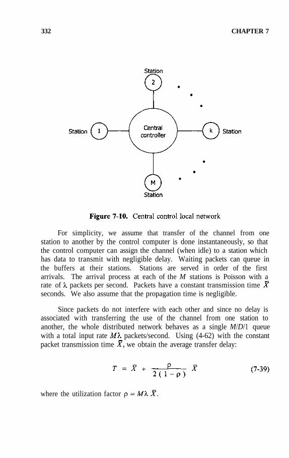
332 CHAPTER 7

For simplicity, we assume that transfer of the channel from onestation to another by the control computer is done instantaneously, so thatthe control computer can assign the channel (when idle) to a station whichhas data to transmit with negligible delay. Waiting packets can queue inthe buffers at their stations. Stations are served in order of the firstarrivals. The arrival process at each of the M stations is Poisson with arate of packets per second. Packets have a constant transmission timeseconds. We also assume that the propagation time is negligible.

Since packets do not interfere with each other and since no delay isassociated with transferring the use of the channel from one station toanother, the whole distributed network behaves as a single M/D/1 queuewith a total input rate packets/second. Using (4-62) with the constantpacket transmission time we obtain the average transfer delay:

where the utilization factor

CHAPTER 7 333

When the channel is busy, it always transmits good packets, andhence, throughput S and utilization factor are equal. Substitution of Sfor into (7-39) yields

Dividing this expression by gives the normalized average transfer delay

Example 7-4. A central control network with channels capacity of64 K bps has 50 stations, each having a Poisson input with a rate of 40packets per minute. Packets have a constant length of 500 bits. Assumethat the propagation time is negligible and the control of use of the channelis instantaneous. What is the average transfer delay on the network?

Solution. The throughput S is given by

Since ms , using (7-40), the average transferdelay is

7-7. SUMMARY

In local area networks, the transmission medium for communicationis shared by many users. To avoid conflicts of access to the transmissionmedium, TDMA, FDMA, and demand assignment techniques may be used.However, for bursty input traffic, random access techniques have been

334 CHAPTER 7

found to be more efficient.

Expressions for determining the average transfer delay in local areanetworks using TDMA, FDMA and CDMA are derived. In general, theaverage transfer delay using TDMA is always smaller than that of usingFDMA or CDMA. It is shown that CDMA and FDMA have the sameaverage transfer delay.

For random access networks, expressions for the throughput and theaverage transfer delay for both the pure ALOHA and the slotted ALOHAare obtained. It is shown that the slotted ALOHA has twice the maximumthroughput as that of the pure ALOHA. By introducing capture capabilityto the ALOHA network, the maximum throughput can be increased further.

For demand assignment with idealized central control access,expressions for the throughput and the average transfer delay are alsodetermined.

REFERENCES

[1] Hammond, J.L. and O’Reilly, P.J.P., Performance Analysis of LocalComputer Networks, Reading Mass.: Addison-Wesley, 1986.

[2] Stallings, W., Local Networks, 3rd ed., New York: Macmillan, 1990.

[3] Hopper, A., Temple, S. and Williamson, R., Local Area NetworkDesign, Reading, Mass.: Addison-Wesley, 1986.

[4] Schwartz, M., Telecommunication Networks: Protocols, Modelingand Analysis, Reading, Mass.: Addison-Welsey, 1987.

[5] Lam, S.S., "Multiple Access Protocols, " in ComputerCommunications, Vol. 1, Principles, ed. Chou, W., Englewood, N.J.:Prentice Hall, 1983.

[6] Frost, V.S. and Melamed, B., "Traffic Modeling forTelecommunications Networks", IEEE Communications Magazine,Vol. 32, No. 3, March, 1994, pp. 70-81.

[7] Leland, W.F., Taqqu, M.S., Willinger, W. and Wilson, D.V., "On theSelf-Similar Nature of Ethernet Traffic", IEEE/ACM Trans. onNetworking, Vol. 2, No. 1, February 1994, pp. 1-15.

CHAPTER 7 335

PROBLEMS

7-1. Each station of a local computer network has an average inputrate of 0.25 messages per second. Messages are 104 bits inlength with no overhead, no retransmissions, and notransmission errors. The channel of the network has a bit rateof 1 Mbps.

(a) How many stations in the network will generate a steady-state unnormalized throughput of 10 messages per second?

(b) What is the normalized throughput S that corresponds to10 messages per second?

7-2. Consider the following two different transmission schemesunder error-free conditions.

Scheme 1: Fifty overhead bits are used for error-correction ineach 250-bit packet; the remaining 200 bits carrydata. Packets are transmitted in a continuoussequence.

Scheme 2: Ten overhead bits are used for error-correction ineach 250-bit packet, the remaining 240 bits carrydata. When each packet is received, a 5-bitacknowledgement message is sent back to thesending station. A new packet is then transmittedafter receipt of the acknowledgement.

Calculate the transmission efficiency for the two schemes.

7-3. A local area network with 120 stations uses a cable with acapacity of 1 Mbps. The network processes packets of 12-bytecharacters. What is the limit on the average input rate inpackets/second of each station if the average transfer delay isless than 0.1 second? We assume that each station has the sameaverage input rate. Obtain a result for a local area network withTDMA protocol and for an idealized central control network.

7-4. A local area network uses a 10 Mbps bus for transmissionmedium. Access to the bus is a fixed assignment protocol.

336 CHAPTER 7

Each station has a Poisson input with a rate of 5 packets persecond. The packet length is 1000 bits. There are 500 stationson the network. Calculate

(a) The mean transfer delay for a FDMA protocol and

(b) The mean transfer delay for a TDMA protocol.

7-5. A local area network supports a number of stations, each ofwhich has a Poisson input with a rate of 0.2 messages persecond. Messages are 2000 bits in length. All stations share acommon channel of bit rate 1 Mbps. If the average transferdelay on the network is limited to 0.1 seconds, what is themaximum number of stations that the network can support byusing (a) a FDMA protocol, and (b) a TDMA protocol.

7-6. An idealized central control network with 100 stations isconstructed with a line of bit rate C = 1 Mbps.

(a) At a throughput of S = 0.4, what is the average messagedelay for 1000-bit messages?

(b) What is the average waiting time in the buffer?

7-7. (a) Assuming that a guardband of g Hz is necessary for eachchannel in an FDMA system, obtain an expression for theaverage transfer delay with 1 bps/Hz modulation. Giveexpressions for the maximum throughput that can beobtained with this system and the fractional increase inthe minimum transfer delay due to the guardbands.

(b) For a channel of total bandwidth 1 MHz and 100 stations,calculate the average transfer delay for an average arrivalrate of 5 packets per second, a guardband of 1 KHz, and1000-bit packet length.

7-8. (a) A TDMA system makes use of extra bits for framesynchronization. Let the fractional overhead time perframe be y. Obtain an expression for the average transferdelay for a TDMA system in terms of the number ofstations M, the throughput S, the average packet

CHAPTER 7 337

transmission time and the overhead factor y. What isthe maximum throughput when the overhead factor isincluded in the analysis?

(b) For a TDMA network with 100 stations and a normalizedthroughput of 0.5, calculate the percentage errorintroduced in the average transfer delay by neglecting theframe overhead when the overhead factor is 0.01.

7-9. A random access network uses the ALOHA accessprotocol. The average input rate to each of the 150stations is 1 packet per second and the packet is ofconstant length of 1000 bits. The channel capacity is 1Mbps.

(a) If the network is operated at this given throughput, whatis the total traffic offered to the network per packettransmission time?

(b) What is the average rate of retransmission per station?

(c) What is the average number of retransmissions persuccessful transmission?

(d) What is the average transfer delay if the backoff strategyis to select an integer from the set {0, 1, 2, • • • , 19}with equal probabilities?

7-10. A slotted ALOHA network has the throughputas given by (7-27). Let the state of the network bedefined by the number of stations with a collided packetwaiting for retransmission. Assume that stations with acollided packet can not generate new packets. When thenetwork is in state k, the throughput is equal to

where is the probability that an idlestation generates a new packet and M is the number of

stations. Suppose that we choose and that a

station with a collided packet will transmit with

probability The average number of attempted

transmissions in a slot when the network is in state k is

338 CHAPTER 7

then equal to

(a) Draw the curve S versus G and the load line; and

(b) Find the intersection of the curve and the load line.

CHAPTER 8

POLLING NETWORKS

8.1. INTRODUCTION

Polling is a method of controlling the access to a transmissionmedium which is shared by a number of stations. A station is a userrequesting service. Polling techniques have been widely used in inquiry -response networks. In polling networks, a controller is required to eitherinitiate or to carry out the polling.

The basic feature of a polling network lies in the action of the centralcontrol computer (controller) in polling each of the stations on the networkin a prespecified cyclic order to provide access to the communicationchannel. Polling networks fall into the class of central control networksdiscussed in Chapter 7.

Messages arriving at each station are first packetized, and then storedin the transmit buffer, where they wait for the poll. As each station ispolled, those stations with packets to transmit can use the full capacity ofthe channel to send their packets to the central computer.

Transmissions between stations take place through the centralcomputer, which receives packets from each station and then transmitsthem to the appropriate stations. The lines connecting the stations and thecentral computer are usually high-speed lines.

Polling networks can operate in either one of two modes: roll-callpolling and hub polling.

For roll-call polling, the central computer initiates the pollingsequence by sending a poll (or polling packet) to a chosen station. Afterthis station has transmitted its packets to the central computer, it notifiesthe central computer with a suffix called go-ahead which is added to its lastpacket. After receiving this suffixed packet, the central computer sends apoll to the next station in the polling sequence, and the process iscontinued.

For hub polling, the central computer sends out a poll to an initialstation in the same manner as for roll-call polling. When this station has

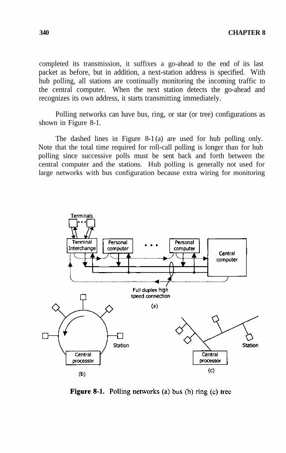
340 CHAPTER 8

completed its transmission, it suffixes a go-ahead to the end of its lastpacket as before, but in addition, a next-station address is specified. Withhub polling, all stations are continually monitoring the incoming traffic tothe central computer. When the next station detects the go-ahead andrecognizes its own address, it starts transmitting immediately.

Polling networks can have bus, ring, or star (or tree) configurations asshown in Figure 8-1.

The dashed lines in Figure 8-1 (a) are used for hub polling only.Note that the total time required for roll-call polling is longer than for hubpolling since successive polls must be sent back and forth between thecentral computer and the stations. Hub polling is generally not used forlarge networks with bus configuration because extra wiring for monitoring

CHAPTER 8 341

between the stations and the central computer is required. However, hubpolling is simpler to implement on local area networks with ringconfiguration.

8-2. OPERATION OF POLLING NETWORKS

This section presents the details for the operation of a pollingnetwork. Both roll-call polling and hub polling are examined as follows.

For roll-call polling, the following sequence of operations is typical:

• The central computer sends out a poll to station i in the pollingsequence;

• Station i receives the poll and reads the station address;

• Station i transmits all of its packets to the central computer;

• Station i appends a go-ahead, and possibly a next-station address,to its last packet;

• The central computer receives all of the packets, including the go-ahead and the next-station address;

• The central computer transmits all of the packets received fromstation i to the destination station; and

• The central computer sends out a new poll to station i + 1 in thepolling sequence.

The above procedures are repeated for each station on the polling list untilall of the M stations have been polled. The whole cycle is then repeatedagain, starting with station i. If a station receives a poll and has no packetto send, it either ignores the poll or sends back a go-ahead with the next-station address to the central computer.

For hub polling, each station with packets to send must add the next-station address following the go-ahead to the last packet of its transmission.If a station has no packet to send, it must send out the go-ahead plus thenext-station address. With this arrangement, the central computer is nolonger needed in transferring the poll between stations. Now each station

342 CHAPTER 8

is continually monitoring the poll.

Note that for both roll-call polling and hub polling, the go-aheadsuffix added to the last packet is necessary, whereas the next-stationaddress is optional for roll-call polling and is required for hub polling.

A polling network may be regarded as a multiple-queue system withcyclic service. Figure 8-2 shows a queueing model for a polling networkwith M stations.

Important measures of performance include the average waiting time,average cycle time, average number of packets in a station queue, andaverage transfer delay.

8-3. PERFORMANCE ANALYSIS OF POLLING NETWORKS

Consider a polling network, where a communication channel is sharedby a number of M stations. At any given time, only one station cantransmit on the network. Because of polling, the channel time iscomprised of two different intervals: the polling interval and the data

CHAPTER 8 343

interval, as shown in Figure 8-3. The polling interval includes all of thetime required to transfer the poll from one station to the next station.

According to the rules for specifying which packets in a given stationare sent during a data interval, services in polling networks may be dividedinto three types: (a) In the exhaustive network, all packets that arrive in astation are sent until the buffer is empty; (b) In the fully gated network,only those packets that arrived prior to the station’s preceding pollinginterval are transmitted; and (c) In the partially gated network, only thosepackets that arrived prior to the station’s data interval are sent.

The arrival intervals for station 0 in the exhaustive, fully gated andpartially gated networks are shown in Figure 8-4.

Average Waiting Time. We shall derive expressions for both theaverage waiting time of a packet before it is transmitted to the centralcomputer, and the average delay time, which is defined as the average timebetween the packet arrival instant at a station and its delivery to the centralcomputer for all the three types of services.

To simplify the analysis, we shall make the following assumptions:

• The network serves M stations, which are numbered 0, 1, ..., M-l.The packet arrival processes of the stations are independent, identical

344 CHAPTER 8

Poisson processes with a rate of packets per second;

• The kth polling interval is used for station k mod M and thesubsequent kth data interval is used to send packets corresponding tothose polling intervals;

• The first and second moments of the packet transmission time areand respectively. The throughput is

• Polling intervals are mutually independent and identically distributedrandom variables with the first and second moments andrespectively; and

• Packets in the transmit buffer of each station are served in the orderof arrival.

Consider the ith packet arriving in the polling network (packets arecounted in the order of arrival, regardless of station). Let

= the residual service time; this is the residual time either for thepacket transmission time or the polling time in progress in thenetwork when the ith packet arrives;

CHAPTER 8 345

= the number of packets in all the M queues in the networkahead of the ith packet; and

= the duration of all the M polling intervals up to the startinginstant of transmission of the ith packet.

Therefore, the waiting time of the ith packet is given by (see Figure 8-5)

where is the transmission time of the jth packet.

Since and are mutually independent random variables, bytaking expectation of the above equation, we have

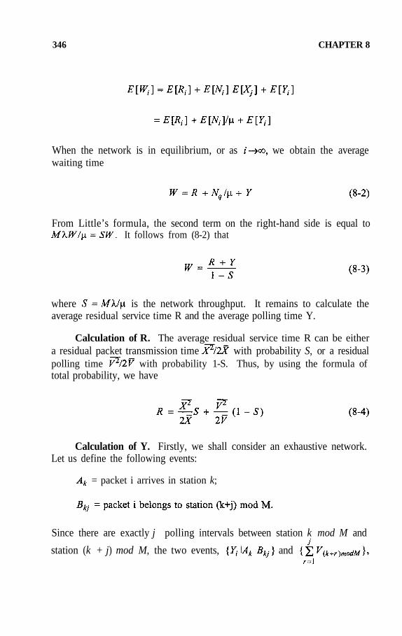
346 CHAPTER 8

When the network is in equilibrium, or as we obtain the averagewaiting time

From Little’s formula, the second term on the right-hand side is equal toIt follows from (8-2) that

where is the network throughput. It remains to calculate theaverage residual service time R and the average polling time Y.

Calculation of R. The average residual service time R can be eithera residual packet transmission time with probability S, or a residualpolling time with probability 1-S. Thus, by using the formula oftotal probability, we have

Calculation of Y. Firstly, we shall consider an exhaustive network.Let us define the following events:

= packet i arrives in station k;

Since there are exactly j polling intervals between station k mod M and

station (k + j) mod M, the two events, and

CHAPTER 8 347

are equivalent. It follows that

and

But

hence,

Furthermore, we have

As we obtain

In the steady state, a packet will arrive at station k with probability 1/M.Using this fact, we obtain

348 CHAPTER 8

Substitution of this probability into (8-6) yields

Combining (8-3), (8-4), and (8-7), we obtain the average packet waitingtime:

Since and (8-8) can be written as

We shall now consider a partially gated network. If a packet arrivesin its own data interval with probability S/M , it will be delayed by anadditional duration of , which is the average sum of polling intervals ina cycle. Thus, Y in (8-7) is increased by and we obtain

Finally, we will consider the fully gated network. If a packet arrivesin its own station data interval, it will be delayed by with probabilityS/M. This is the same as the partially gated system. However, if a packetarrives in its own polling interval, it will be delayed by withprobability (1 – S)/M. Thus, Y in (8-7) is increased by an additional

delay, We then obtain

CHAPTER 8 349

Having determined the average waiting time, it is straight-forward tofind the average number of packets in a station transmit buffer. UsingLittle’s formula directly, the average number of packets in a station bufferis given by

where W is given by (8-9), (8-10), or (8-11).

Example 8-1. Consider a metropolitan area network with a centralprocessor (controller) located at the headend of a broadband CATV(community antenna or cable television) network that has a tree topology.The network has the following characteristics:

• Maximum distance from headend to a subscriber station = 20 km;

• Number of subscribers = 1000;

• Length of go-ahead = 1 byte or 8 bits;

• Length of polling packet = 8 bytes;

• Access technique is roll-call polling;

• Data rate of channel = 56 Kbps;

• Propagation time

• Packet length distribution for packets from subscriber to headend isexponential with mean of 100 bytes; and

• Modem synchronization time = 5 ms.

Assume that the network is operated in exhaustive mode.

350 CHAPTER 8

(a) If each user generates packets at a rate of one packet per minute,what is the mean waiting time?

(b) If the number of subscribers is increased to 1500, what is thecorresponding mean waiting time?

(c) Calculate the average number of packets in each station queue forparts (a) and (b).

Solution. For roll-call polling, the mean polling time for each stationconsists of the modem synchronization time, the transmission times of go-ahead and of the polling packet, and the propagation times from a stationto the headend processor and from the headend processor to the nextstation.

Modem synchronization time = 5 ms.

Transmission times of go-ahead and polling packet

= 1.2857 ms.

Maximum one-way propagation time ms

Thus, the mean polling time is

ms.

(a) Mean packet transmission time

Mean polling time ms

Total throughput

Since the packet length distribution is exponential and the polling time isconstant, we have

CHAPTER 8 351

and Using these results in (8-9), we obtain

seconds

(b) Now M = 1500 subscribers;

Thus, seconds

(c) For part (a), the average queue length is

packets

For part (b),

Average Cycle Time. The total time required to poll all of thestations and to return to the starting station in the polling sequence is calledthe cycle time. The cycle time depends on the number of packets to betransmitted by each station after the last poll and hence is a randomvariable. The average cycle time is an important parameter fordescribing the operation of polling networks.

Let be the average number of packets that arrive at a station in anaverage cycle time From Little’s formula, we obtain

Since the average packet transmission time is and the average pollinginterval is the average cycle time can be expressed as

By combining these two equations, we obtain the average cycle time:

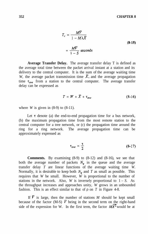
352 CHAPTER 8

Average Transfer Delay. The average transfer delay T is defined asthe average total time between the packet arrival instant at a station and itsdelivery to the central computer. It is the sum of the average waiting timeW, the average packet transmission time and the average propagationtime from a station to the central computer. The average transferdelay can be expressed as

where W is given in (8-9) to (8-11).

Let denote (a) the end-to-end propagation time for a bus network,(b) the maximum propagation time from the most remote station to thecentral computer for a tree network, or (c) the propagation time around thering for a ring network. The average propagation time can beapproximately expressed as

Comments. By examining (8-9) to (8-12) and (8-16), we see thatboth the average number of packets in the queue and the averagetransfer delay T are linear functions of the average waiting time W.Normally, it is desirable to keep both and T as small as possible. Thisrequires that W be small. However, W is proportional to the number ofstations in the network. Also, W is inversely proportional to 1 – S. Asthe throughput increases and approaches unity, W grows in an unboundedfashion. This is an effect similar to that of on T in Figure 4-8.

If is large, then the number of stations M should be kept smallbecause of the factor (M-S) being in the second term on the right-handside of the expression for W. In the first term, the factor would be at

CHAPTER 8 353

a minimum if the packet length is constant and equal to for

Example 8-2. For the metropolitan area network of Example 8-1with 1000 subscribers, calculate (a) the average cycle time, and (b) theaverage transfer delay.

Solution.

(a) M = 1000, ms. S = 0.238, using (8-15), we find the meancycle time

(b) Since W = 4.2622 seconds,

then applying (8-16) yields

8-4. SUMMARY

This chapter presents the operation of roll-call and hub pollings. Apolling network may be considered as a multiple-queue with a cyclicserver. Because of polling, the channel time for each station is comprisedof a polling interval and a data transmission interval.

For performance analysis, we obtain expressions for the mean waitingtime of exhaustive, partially gated, and fully gated polling networks. Fromthese mean waiting times, the corresponding average transfer delays arealso obtained.

Furthermore, we derive an expression for the average cycle time. It shouldbe pointed out that the queueing model for the analysis of polling networkscan also be used for the analysis of ring networks, as will be discussed

354 CHAPTER 8

with modifications in the next chapter.

REFERENCES

[1] Hammond, J.L. and O’Reilly, P.J.P., Performance Analysis of LocalComputer Networks, Reading, Mass.: Addison-Wesley, 1986.

[2] Bertsekas, D. and Gallager, R., Data Networks, 2nd ed., EnglewoodCliffs, N.J.: Prentice Hall, 1992.

[3] Schwartz, M., Telecommunication Networks: Protocols, Modelingand Analysis, Reading, Mass.: Addison-Wesley, 1987.

[4] Takagi, H., Analysis of Polling Systems, Cambridge, Mass.: MITPress, 1986.

PROBLEMS

8-1. Consider the pairs of multidrop telephone lines which connectone primary node to a number of secondary nodes. The signaltransmitted by the primary node passes through a pair of wiresand is received by all of the secondary nodes. Similarly, thereis a return pair of wires which carries the sum of the transmittedsignals from all of the secondary nodes to the primary node.The mode of operation for multidrop telephone lines is for theprimary node to poll each secondary node in some order. Eachsecondary node responds to its poll either by sending data backto the primary station or by indicating that it has no data tosend. Data for the network are as follows:

• Maximum distance between the primary station and thefurthest secondary stations is 10 km;

• Propagation time is 5 per km;

• Modem synchronization time is 20 milliseconds;

• Length of go-ahead is 1 byte;

• Length of polling packet is five 8-bit bytes;

CHAPTER 8 355

• Bit rate of the channel is 96 kbps;

• Exponential packet length with average length of 100bytes;

• Input to each station is independent Poisson with anaverage rate of 1 packet per minute; and

• Assume exhaustive mode.

(a) What is the maximum number of stations such that theaverage transfer delay is at most one second?

(b) What is the maximum number of stations for a normalizedthroughput equal to 0.5?

8-2. A polling network is to be constructed with hub polling and thedata listed below:

• Go-ahead message is two 8-bit bytes;

• Synchronization time for go-ahead is 5 ms ;

• Constant packet length equals 500 bits;

• Independent Poisson input with average rate to each stationis 1 packet per minute;

• Number of stations is 200;

• Propagation time is negligible; and

• Bit rate of channel is 2400 bps.

(a) What is the minimum bit rate for the operation of thenetwork to be stable?

(b) Calculate the average transfer delay for the exhaustive,fully-gated and partially-gated operations.

(c) What is the mean cycle time?

356 CHAPTER 8

8-3. Design a (roll-call) polling network with 10 stations, 200 metersapart with one station 200 meters from a central computer.Each station is to service 10 terminals, whose inputs are allindependent Poisson processes with average rates varying from1-10 messages per minute. Each message is fifty 8-bit byteslong and the messages are transmitted by the stations to thecentral computer. The terminals transmit messages into a bufferat a station over a 1 kbps line, where the messages are storeduntil the station can transmit to the central computer. Aspecification for the design is that the total average transferdelay for messages from a terminal to the central computer mustnot exceed one second. Assume that the go-ahead message andthe polling message are respectively 1 byte and 3 bytes long,while the propagation time is 5 . Assume exhaustiveoperation.

8-4. M stations 100 meters apart are connected to a bus in tandemwith 100 meters between the nearest station and the centralcomputer. The connections are all made with 20 kbps lines.Messages transmitted from stations to the central computer areall 500 bits long. Each station serves 30 terminals, each ofwhich generates independent Poisson traffic with an average rate

of 1 message per minute. Modem synchronization time is 10milliseconds, propagation delay is 5 per kilometer, pollingpackets are five 8-bit characters, and the go-ahead is two 8-bitcharacters. Assume exhaustive operation:

(a) How many stations can be serviced if the total averagetransfer delay for messages from the stations to the centralcomputer must be less than 1 second?

(b) What is the minimum value of total average transfer delayas the throughput approaches zero? Given theconfiguration of stations, how can this transfer delay bereduced?

(c) What is the absolute limit on the number of stations to beserviced by the network?

8-5. Show that for both the fully-gated and partially-gated pollingnetworks, the steady-state probability of a polling interval being

CHAPTER 8 357

followed by an empty data interval is Hint: If

p is the required probability, argue that the ratio of the times

used for data intervals and for polling intervals is

CHAPTER 9

RING NETWORKS

9-1. INTRODUCTION

A ring network is a local area network which consists of a number ofrepeaters joined by point-to-point links to form a closed loop. The repeateris a device, capable of receiving data on one link and transmitting it, bit bybit, on the other link as fast as it is received with no buffering. The linksare unidirectional so that data are transmitted in one direction only aroundthe ring, and can be read by all stations attached to the ring (Figure 9-1,see p. 358).

CHAPTER 9 359

information, including the destination station address. These packets arestored in the station transmit buffer when awaiting transmission on thering.

For a ring network to operate as a communication network, threefunctions are required: data insertion, data reception, and data removal. Inaddition to serving as an active transceiver on the ring, each repeater alsoserves as a device for data insertion.

A number of different types of ring networks has been designed andimplemented. Of the many different types of rings proposed, three typesdeserve more attention: token rings, slotted rings, and register insertionrings.

This chapter presents performance analysis of the above mentionedthree types of rings in detail. The main performance measure for ringnetworks is the mean packet delay. Thus, performance analysis consists ofdetermining the mean packet delay, and how it is affected by the variousparameters of the network, such as statistics of the packet service time, thenetwork throughput, and the number of stations.

9-2. TOKEN RING NETWORKS

When a station has data to send, it first carries out the packetization,stores the packets in the transmit buffer and waits for the free token whichcontrols the access to the ring for transmission. When this station’srepeater receives the free token, the repeater retransmits the bits receivedfrom the station on the outgoing link. During this period of transmission,bits may arrive on the incoming link. In this case, there are twopossibilities that are treated differently:

1. If the packet length is longer than the bit length of the ring (theround-trip delay in bit times often called the ring latency), the bitscould be from the same packet that the repeater is still sending. Therepeater passes the bits back to the station, which can check them asa form of acknowledgement.

2. For multiple-token rings, more than one packet could be on the ringat the same time. If the repeater, while transmitting, receives bitsfrom a packet it did not originate, it must store them in a buffer forlater transmission.

360 CHAPTER 9

A packet may be removed by the repeater of the destination station orby the transmitting station’s repeater after it has made a round trip on thering. The latter approach is more desirable because it permits automaticacknowledgement and multicast addressing (one packet being sent tomultiple stations).

The repeater on the ring network serves two main purposes: tomaintain the proper functioning of the ring by passing on all the datacoming from the incoming link and to provide an access point for theattached stations to send and receive data.

The most important feature of the ring structure is that it uses point-to-point communication links. This fact brings a number of advantages:

• Since the transmitted signal is regenerated at each node, greaterdistances can be covered;

• The ring structure can accommodate optical fibre links;

• Implementation is simple because transmission paths are fixed;• Routing algorithms are not required;

• Stations introduce only a small delay to a packet circulating on thering; and

• Multiple addressing is straightforward.

Disadvantages, on the other hand, are:

• Reliability is not good because a failure of an interface unit or a linesegment can cause a breakdown on the ring;

• The ring must be broken to add or delete stations so that it isinflexible;

• Propagation delay is proportional to the number of stations on thering; and

• There is a practical limit to the number of repeaters on a ring.

9-3. OPERATION OF TOKEN RING NETWORKS

Token ring is a medium access control technique for ring networksoriginally proposed by W.D. Farmer and E.E. Newhall in 1969, andreferred to as the Newhall ring. It is based on the use of a small frame,called a token, which is a distinctive bit pattern. The token circulates

CHAPTER 9 361

around the ring from station to station and can be in one of two possiblestates: idle or busy. When the ring is first activated or initialized, an idle(or free) token is inserted in the ring. A station with data to transmit mustwait until it seizes the idle token and changes it to busy state beforetransmitting. The busy token then becomes part of the header of datatransmitted on the ring by the station repeater. Thus, other stations on thering can read the header, detect the busy token, and refrain fromtransmitting. The busy token on the ring will make a round trip and beremoved by the transmitting repeater. When the station has completedtransmission of its data and the first bit of its transmitted data has returnedto the station (after a round trip), the transmitting station inserts a new free(or idle) token on the ring. Thus, the use of a token guarantees that onlyone station may transmit at a time.

In an elementary ring network, the token can be a distinctive patternof several bits. In more sophisticated ring networks, such as the IEEE 802token ring, the token can be several bytes long. For a simple token whichcould be a sequence of eight 1’s, to prevent the occurrence of this bitpattern in the data, it is necessary to use the bit stuffing technique. Whenbit stuffing has been used, the receiver must be able to identify the added(stuffed) bits, so that they can be removed before error detection.

A long dedicated bit pattern with bit stuffing can be inefficient. Analternative is to use special bits for the token, or special bits to mark thebeginning and ending of a control field. For example, Manchester codingmay be used for data with violations for control bits.

Logical operation of the repeater (interface unit) is shown in Figure9-2. There are two modes: the listen mode and the transmit mode.Stations are normally in the listen mode, in which the station can read theaddress of the data circulating on the ring and copy the contents of packetsaddressed to it. Otherwise, the station retransmits each bit with a smalldelay. When the station has data to send and when its repeater seizes afree token, the repeater receives bits from the station and retransmits themon its outgoing link to the ring after changing the free token to busy state.

There are two types of transmission schemes: the exhaustive serviceand nonexhaustive service. For the exhaustive service, the station transmitsall the data stored in the transmit buffer and then places a new free tokenon to the ring. For nonexhaustive service, the station is allowed totransmit only a specified number of packets each time it captures a free

362 CHAPTER 9

token. In both service schemes, the transmitting station repeater isresponsible for removing its data from the ring. In the sequel, theexhaustive type of operation is assumed.

Station Latency. In a ring network, bits are transmitted serially outof each station interface. Normally, the input to each repeater is the outputof the previous repeater delayed by the propagation time between the twostations. In the listen mode, each repeater passes on the data received fromits incoming link at the input after a delay known as the station latency.The station latency can be a minimum of one bit time or a dozen of bittimes. Let this delay be b bit times and the channel capacity be C bps.The station latency is given by

Ring Latency. Bits circulate around the ring in a synchronousfashion. If all the repeaters are in the listen mode, the token circulatesaround the ring in a time equal to the sum of the propagation delays plusthe sum of the station latencies. This composite time is called the ringlatency.

CHAPTER 9 363

Let be the round-trip propagation delay for the ring and M be thenumber of stations on the ring. The ring latency is given by

Depending on when a new free token can be generated, there arethree operational modes which are referred to as multiple-token operation,single-token operation, and single-packet operation.

Multiple-Token Operation. For multiple-token operation, thetransmitting station repeater places a new free token on the ringimmediately following the last bit of the transmitted packet. This type ofoperation permits several busy tokens and one free token on the ring at anygiven time. With more than one token on the ring, packet lengths andstation latencies must be related, so that busy tokens do not progress farenough around the ring to be removed by their originating station beforethe new free token is generated.

Single-Token Operation. For single-token operation, a transmittingstation generates a new free token only after it has removed its own busytoken. If a packet length is longer than the ring latency in bit times, thetransmitting station will remove its busy token before it finishestransmitting data. In this case, the station must continue transmitting dataand generate a new free token only after the last data bit has beentransmitted. This situation is exactly the same as the multiple-tokenoperation. Thus, single-token and multiple-token operations differ only incases of packet lengths being shorter than the ring latency.

Single-Packet Operation. For single-packet operation, a transmittingstation generates a new free token only after both its busy token and all ofits transmitted data have circulated a round-trip on the ring and arecompletely removed from the ring. This type of operation ensures that twotransmissions will not interfere each other.

To illustrate the three types of operations, consider a four-stationtoken ring network with 1 bit time delay per station and negligiblepropagation delay (Figure 9-3). We assume that initially station 1 receivesa free token at t = 1 and outputs a busy token at t = 2. Note that the ringlatency is four bit times.

364 CHAPTER 9

At t = 5, after traversing the ring with a ring latency of four bittimes, the busy token and the transmitted data of station 1 begin to returnto station 1 and hence are removed. As shown in Table 9-1, in all threetypes of operations, station 1 initially transmits a packet of total length sixbit times at t = 1 and station 4 transmits a packet of total length three bittimes.

Note that the time at which a free token is subsequently generateddepends on the mode of operation. Specifically, a new free token isgenerated by station 1 at t = 8 and by station 4 at t = 14 for multiple-token operation; by station 1 at t = 8 and by station 4 at t = 15 forsingle-token operation; and by station 1 at t = 11 and by station 4 at t=20for single-packet operation.

CHAPTER 9 365

9-4. PERFORMANCE ANALYSIS FOR TOKEN RINGNETWORKS

Packets generated at a station are stored in the transmit buffer andwait for the free token. In addition to the waiting time, the packet hasthree more delays before it arrives at its destination station:

1. The delay due to station latency;

2. The propagation delay associated with each link segment of the ringthe packet traverses from originating station to destination station; and

366 CHAPTER 9

3. The transmission time of all the bits in the packet over the links ofthe ring.

We shall derive expressions for the average transfer delay suffered bypackets on token ring networks for multiple-token, single-token, andsingle-packet operations.

To simplify the analysis. we make the following assumptions:

• The arrival process to each station is an independent Poisson processwith a rate of packets/second;

• The average distance between the sending and receiving stations isone-half of the distance around the ring;

• There are M stations which are spaced so that the propagation delaybetween two consecutive stations is equal to where is thering latency;

• The packet length distribution is the same for each station, with meanbits and second moment where the random variable L

denotes the length of an arbitrary packet. The channel capacity is Cbps so that the packet transmission time has the same distribution asL with mean seconds and second moment(seconds)2; and

• Service at each station is of the exhaustive type.

To determine the average transfer delay for token ring networks, notethe similarity between the operation of the token ring and the hub pollingnetworks, as discussed in Chapter 8 (see also Figure 8-2(b) and Figure 9-1). The fact that hub polling typically requires a central controller,whereas token ring does not, does not make any difference in performanceanalysis. Operation of both networks is essentially the same.

The average time between the instant a station finishes itstransmission of packets and the instant the next station receives a freetoken corresponds to the average polling interval. Thus, we adapt theaverage waiting time in a polling network, given by (8-9), for the tokenring network. This equation is rewritten here, with constant and

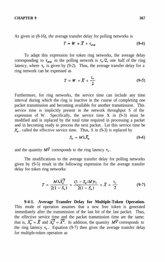
CHAPTER 9 367

As given in (8-16), the average transfer delay for polling networks is

To adapt this expression for token ring networks, the average delaycorresponding to in the polling network is one half of the ringlatency, where is given by (9-2). Thus, the average transfer delay for aring network can be expressed as

Furthermore, for ring networks, the service time can include any timeinterval during which the ring is inactive in the course of completing onepacket transmission and becoming available for another transmission. Thisservice time is implicitly present in the network throughput S of theexpression of W. Specifically, the service time X in (9-3) must bemodified and is replaced by the total time required in processing a packetand in becoming ready to process the next packet. Let this service time be

, called the effective service time. Thus, S in (9-3) is replaced by

and the quantity corresponds to the ring latency

The modifications to the average transfer delay for polling networksgiven by (9-5) result in the following expression for the average transferdelay for token ring networks:

9-4-1. Average Transfer Delay for Multiple-Token Operation.This mode of operation assumes that a new free token is generatedimmediately after the transmission of the last bit of the last packet. Thus,the effective service time and the packet transmission time are the same;that is, and In addition, the quantity corresponds tothe ring latency Equation (9-7) then gives the average transfer delayfor multiple-token operation as

368 CHAPTER 9

where From (9-8), we see that if then the third termon the right-hand side has the dominating effect on the average transfer

delay T.

9-4-2. Average Transfer Delay for Single-Token Operation. Inthis mode, a new free token is generated only when the transmitting stationhas received its own busy token after a round trip. Thus, there can be onlyone token on the ring at any one time.

If the packet transmission time is greater than the ring latencythe station is still transmitting when its busy token returns after a roundtrip. Thus, it cannot generate a new free token until it has finished thetransmitting packet, and the operation is completely identical to that ofmultiple-token operation.

On the other hand, if the packet transmission time is less than thering latency, single-token operation can be different from multiple-tokenoperation because the effective service time is greater than the packettransmission time X due to periods when the transmitting station is waitingfor the busy token to return. During these periods the whole network istied up by the busy token.

For single-token operation, the relationship between the packettransmission time X and the ring latency is of central importance. Weshall consider the cases of fixed packet transmission time and exponentiallydistributed packet transmission time separately.

For fixed packet transmission time, X = constant Thus, asnoted previously, if the single-token operation is exactly thesame as the multiple-token operation, and hence the average transfer delayT is given by (9-8) with If however, the single-token operation becomes different from the multiple-token operation sincethe effective service time Thus, andfor the ring cannot be used to transmit a new packet until the busy tokenof the previous packet has circulated completely around the ring.

CHAPTER 9 369

With (9-6) becomes

where

Substitutions of and in (9-9) into (9-7) yield the averagetransfer delay for single-token operation as

For exponentially distributed packet transmission times with meanthe distribution function is given by

It follows that the effective service time has the distribution function

the density function

370 CHAPTER 9

the first moment

and the second moment

The results of (9-13) and (9-14) together with Se as given by (9-9) can besubstituted in (9-7) to obtain the average transfer delay:

9-4-3. Average Transfer Delay for Single-Packet Operation. Inthe single-packet mode, the sending station generates a new free token onlywhen it has received and removed all of the packets it has transmitted.Thus, there is never more than one packet circulating on the ring. In thiscase, there is always a delay of seconds after the complete transmissionof each packet so that the effective service time is The first andsecond moments of this effective service time are, respectively,

and

Using (9-16) and (9-17) together with (9-6) in (9-7) yields an expressionfor the average transfer delay for single-packet operation as

CHAPTER 9 371

Example 9-1. Consider a single-token ring that has the following givenparameters:

• One hundred stations on the ring;

• Ring length of 1 km;

• Ring bit rate of 10 Mbps;

• Mean packet length of 1000 bits;

• Independent Poisson arrival process to each station with a rate of 10packets/second;

• Station latency of 2 bits; and

• Propagation delay of the ring of 5 µs per km;

(a) Determine the mean transfer delay for both constant and exponentialpacket lengths.

(b) If the number of stations on the ring is increased to 200 and thePoisson arrival rate is increased to 25 packets per second, calculatethe mean transfer delay. All the other network parameters areunchanged.

(c) Repeat calculations in (b) for station latency of 5 bits.

Solution

(a) For constant packet length,

M = 100, packets per second,

Since using (9-8) yields

372 CHAPTER 9

or 0.132 ms

For exponential packet length,

or 0.1375 ms

(b) Now, M = 200 and packets/second. Then

For constant packet length, (9-8) yields

ms

For exponential packet length, (9-8) yields

or 0.2675 ms

(c) Since bits, the ring latency becomes

Using (9-10) for constant packet length, we find

or 0.3208 ms

For exponential packet length, using (9-15) yields

or 0.5384 ms

CHAPTER 9 373

9-5. OPERATION OF SLOTTED RING NETWORKS

Suppose that traffic on a ring is uniformly distributed betweendifferent source-destination pairs. It can be conceived that, on average, apacket need be transmitted to only half of the links of a ring network.Since, in the token ring network, a packet travels on every link, we see thathalf the network’s transmission capacity is wasted. It is therefore possibleto achieve twice the throughput, at least in principle, by using a differentcontrol strategy. Slotted rings and register insertion rings are suchstrategies that allow higher throughput.

The slotted ring control strategy is based on the empty slot principle.In the slotted ring, a number of fixed length slots circulate continuously onthe ring, each slot containing a leading bit to indicate the slot as empty orfull (Figure 9-4). This strategy was first proposed by J. Pierce and isreferred to as the Pierce loop. Most of the development work on thistechnique was done at the University of Cambridge in England and it isknown as the Cambridge ring.

All slots are initially marked empty. A station with data to send mustbreak the data up into fixed-length packets called minipackets. It thenwaits until an empty slot arrives, marks the slot full, and inserts aminipacket of data as the empty slot goes by. To prevent hogging of thering by one station (a phenomenon that a station may use more than its fairshare of the empty slots for transmission), the sending station is notallowed to transmit another minipacket until its full slot makes a completeround trip, to be marked empty again by the sending station.

To illustrate the operation of a slotted ring, let us consider the four-station slotted ring in Figure 9-5. One of the stations, say, station 2, is themonitor station which is used to set up and maintain ring packetizing andto perform error checks. Each station has a latency of one bit.Propagation delay is ignored and the 4-bit latency is used to support oneslot on the ring. The first bit of the 4-bit slot is used as the empty/fullindicator. The operation is illustrated in Table 9-2 for two operatingconditions: when only one station has data to transmit and when twostations have data to transmit.

When only station 1 has data to transmit, it captures the empty slot att = 0, marks the slot full at t = 1 and inserts a minipacket of data, andthen releases the ring by marking the full slot to empty at t = 5. Since the

374 CHAPTER 9

other three stations do not have data to transmit, station 1 can send anotherminipacket only until t = 8. In this case, station 1 can make use of thering only one-half of the time. This can be seen from the station 1 columnin the table.

When stations 1 and 3 have data to transmit, the operation of theslotted ring is shown on the right-hand half of the table. Unlike theprevious case, the outputs of all four stations at any one time are neverempty. This can be observed by examining the rows in the table.

For slotted ring networks, the ring latency determines the totalnumber of bits in the circulated slots. This fact has an important influenceon the design of a slotted ring. For example, consider a 10 Mbps channel.The bit time is 0.1 A typical channel propagation delay is 5 perkilometer so that one kilometer of cable can support 50 bits. If eachstation introduces a latency of 1 bit, then either a large number of stationsor a long cable is required. Suppose that the ring has 100 stations

CHAPTER 9 375

connected by 2 kilometers of cable. The ring latency is equal to2 × 50 + 100 × 1 = 200 bits. This ring can then support four slots of 50bits, ten slots of 20 bits, etc.

9-6. PERFORMANCE ANALYSIS FOR SLOTTED RINGNETWORKS

To derive an expression for the average transfer delay in a slottedring network, we make the following assumptions:

• Input data traffic to each station is an independent Poisson arrivalprocess with a rate of packets/second;

• There are M stations on the network. Each station has a latency ofseconds;

376 CHAPTER 9

• The propagation delay around the ring is seconds and the ringlatency is equal to

• The packet transmission times are mutually independent andidentically distributed with the first and second moments andrespectively;

• The minipacket length is much smaller than the packet length;likewise, the minipacket transmission time is much smaller than thepacket transmission time; and

• The bit rate on the channel (ring) is C bps.

Since the time for a slot to circulate around the ring is very small (incomparison to a packet transmission time), it will be ignored in theanalysis. Based on the above assumptions, the slotted ring network can be

CHAPTER 9 377

modeled as a distributed M/G/1 queueing system with arrival rate andgeneral service time with first moment and second moment

We modify (9-5) to represent the average transfer delay for theslotted ring network and rewrite it as

where the average waiting time W is given by the Pollaczek-Khinchinformula (4-61)

Since the throughput is given by

we replace by S in (9-20) to yield

To take into account the large amount of overhead used in eachminipacket for the slotted ring network operation, we let be the numberof header bits contained in each slot and be the number of data bits ineach slot. Then is the length of each slot in bits. Define theoverhead factor

From this, we see that the effective packet transmission time is increased toseconds in a slotted ring network. It follows that the effective

throughput is also increased to (1 + h)S.

378 CHAPTER 9

Introducing these changes to (9-19) and (9-22) then gives the averagetransfer delay for the slotted ring network as

As illustrated in Figure 9-5, for the actual operation of the slottedring network, on average, a packet only needs to traverse half of the ring,since the effective channel bit rate as seen by any particular station is onlyhalf of the links of the ring. This implies that the packet transmission time

is effectively With this modification, we write (9-24) as

It is important to note that for a slotted ring, the number of slots onthe ring m, the gap time g in seconds, the minipacket size in bits,the channel bit rate C in bps, the propagation delay around the ring inseconds, the number of stations M, the station latency in seconds, andthe ring latency in seconds are related by the following expression

In the design of a slotted ring network, the number of slots m isusually adjusted so that the gap g is minimized. If the station latencies arenot sufficiently large to provide the required ring latency additionalartificial delays can be added in the station latency Some of the ideasare illustrated by the following example.

Example 9-2. Consider a slotted ring of 1 kilometer in length with 50stations. Each station has a latency of 1 bit. The slot size is 6 bytes with3 bytes data. The channel bit rate is 10 Mbps and the propagation delayon the ring is 5 per kilometer.

(a) How many slots can the ring hold without adding any artificialdelays? What is the gap time? If the packet size is a constant of1200 bits long, what is the average transfer delay when the packet

CHAPTER 9 379

arrival rate at each station is (i) 10 packets per second, (ii) 40 packetsper second?

(b) If the number of stations is increased to 100, how many slots can thering hold without adding artificial delays? What is the gap time?What is the average transfer delay for each of the two arrival rates in(a) with the same constant packet length of 1200 bits?

Solution

(a) Using (9-26), the ring latency is given by

and for the slot size of 6 bytes,

We see that the largest integer that makes less than or equal to 10 ism = 2. As a result, the gap timeThe overhead factor is given by

The packet transmission time is

(i) For packets/second,

Since the packet length is constant, using (9-25) gives theaverage transfer delay

380 CHAPTER 9

(ii) For packets/second,

and

(b) For 100 stations, the ring latency is increased to

Now the number of slots m on the ring can be three with a gap timeof 0.6 .

(i) For packets/second,

and

(ii) For packets/second,

and

CHAPTER 9 381

Observe that from (9-25), the maximum throughput is

The average transfer delay will be very large when S is close toUnder light and medium load conditions, say, the dominant factorin the average transfer delay is the second term, on the right-hand side of (9-25). When the first term becomes dominant.

9-7. REGISTER INSERTION RINGS

The register insertion ring derives its name from the shift register inthe interface of each station on the ring. The shift register, equal in size tothe maximum packet length, is used for temporarily holding packets thatcirculate past the station. In addition, the station also has a transmit bufferfor storing locally generated packets and a receive buffer for storing theinput traffic of the station.

The distinctive structure of the interface is shown in Figure 9-6. Theaddition of the shift registers into the ring effectively increases the capacityand hence the throughput of the ring in terms of the total number of bits itcan hold at any one time.

9-8. OPERATION OF REGISTER INSERTION RING NETWORKS

Operation of the register insertion ring can be described by theinterface shown in Figure 9-7. First, consider the case in which the stationhas no data to send and the receive and transmit switches in Figure 9-6 arein position A. Bits circulate around the ring through the insertion buffer inthe same way as for a slotted ring. When the insertion buffer is empty, theinput pointer is at the rightmost position. When bits arrive from the ring,they are inserted bit by bit in the insertion buffer, with the input pointershifting left for each bit. As soon as the full address field is in theinsertion buffer, the station can determine if it is the addressee. If not, thepacket is forwarded to the ring until the packet is gone. Now, if no furtherpackets arrive, the input pointer will return to its initial rightmost position.

382 CHAPTER 9

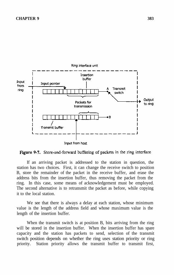
CHAPTER 9 383

If an arriving packet is addressed to the station in question, thestation has two choices. First, it can change the receive switch to positionB, store the remainder of the packet in the receive buffer, and erase theaddress bits from the insertion buffer, thus removing the packet from thering. In this case, some means of acknowledgement must be employed.The second alternative is to retransmit the packet as before, while copyingit to the local station.

We see that there is always a delay at each station, whose minimumvalue is the length of the address field and whose maximum value is thelength of the insertion buffer.

When the transmit switch is at position B, bits arriving from the ringwill be stored in the insertion buffer. When the insertion buffer has sparecapacity and the station has packets to send, selection of the transmitswitch position depends on whether the ring uses station priority or ringpriority. Station priority allows the transmit buffer to transmit first,

384 CHAPTER 9

whereas ring priority gives preference to the insertion buffer.

The principal advantage of the register insertion technique is highthroughput by allowing multiple packets on the ring. However, thisrequires the recognition of an address prior to removal of a packet. If apacket’s address field is damaged, it could circulate the ring indefinitely.

9-9. PERFORMANCE ANALYSIS OF REGISTER INSERTIONRING NETWORKS

For register insertion ring networks, the performance criterion is theaverage transfer delay on the network measured from the time the packet isstored in the transmit buffer to the time the packet is received by thereceive buffer of the destination station. The times required to move thepacket from the sending station to the transmit buffer and from the receivebuffer to the receiving station are not included in the calculation.

To develop a model for performance analysis, we make the followingassumptions:

• The packet arrival process to each station’s transmit buffer is Poissonwith rate

• The packet transmission times are mutually independent andidentically distributed random variables with first and secondmoments and respectively;

• There are M stations on the network. Each station has a constantlatency of seconds;

• All stations have the same traffic pattern: a station transmits toanother station with k-separation (measured by the number of linksbetween them) with probability qk , k = 1, 2, • • • , M – 1; thisassumption implies that the probability of transmission between anytwo stations depends only on the separation of the two stations;

• The capacity of all buffers is infinite; and

• The packet interarrival times and service times are mutuallyindependent; thus, each station can be modeled independently.

CHAPTER 9 385

Figure 9-8 depicts a queueing model for the interface of Figure 9-6.A simplified model is shown in Figure 9-9 subject to the above sixassumptions.

386 CHAPTER 9

In the simplified model it is assumed that the input process to theinsertion buffer is Poisson with rate which remains to be determined.Intuitively, it can be observed that depends on and because isthe sum of a portion of the generated traffic from the other M-lstations.

First, we observe that a packet may wait in only one (transmit) bufferof the source station and does not go through the insertion buffer of eitherthe source station or the destination station. Second, consider a test station,say, station 1 for convenience. According to assumption 4, the traffictransmission pattern of this test station can be represented by the traffictransmission diagram of Figure 9-10. The numbered circle denotes astation. Since a packet can be sent to only M-l possible stations, eachwith probability which is measured by the separation, it follows that

Note that the traffic transmission pattern shown in Figure 9-10 is valid andis the same for each station, although the order of the stations may bedifferent.

Now let us calculate the total transit traffic at station M, contributed by all

CHAPTER 9 387

the other M-1 stations. Figure 9-11 shows the contribution of transit trafficfrom each of the other M-1 stations, where only the transit traffic of eachstation (except station M) is depicted.

Like traffic transmission, the transit traffic shown in Figure 9-11 is thesame for each station. By summing all the transit traffic at station M, weobtain

388 CHAPTER 9

where, in the third step, (9-27) has been used in the first term on the right-hand side.

Introducing a new notation

the last expression can be written as

The quantity a can be regarded as the average number of insertion bufferstraversed by a packet. Having determined the arrival rate for theinsertion buffer, the simplified model in Figure 9-9 can be regarded as ahead-of-the-line nonpreemptive priority M/G/1 queueing system. It shouldbe noted that service in the simplified model and in the queueing model ofFigure 9-8, is different from the normal queue in that service is defined tooccur only in the receive buffer of the destination station.

CHAPTER 9 389

The simplified model in Figure 9-9 can now be used to determine theaverage waiting times in the transmit queues and in the insertionqueues, under both ring and station priority conditions. The resultsobtained in (4-88) and (4-89) of Chapter 4 can be used to calculate and

depending on which queue is given priority.

Case 1. Ring Priority (priority to insertion buffer)

For this case, we replace quantities with subscripts 1 and 2 byquantities with subscripts r and t in (4-88) and (4-89), respectively, to give

and

where

and

390 CHAPTER 9

Case 2. Station Priority (priority to transmit buffer)

In this case, the expressions (9-29) and (9-30) are interchanged toaccount for the interchange in priority, to give

and

Now consider the average packet transfer delay for the registerinsertion ring. We observe that the average delay consists of fourcomponents: the average delay (waiting time) in the transmit bufferthe average packet transmission time the average station latencytraversed by a packet and the average waiting delay due toinsertion buffers . Adding all these four components gives the averagetransfer delay as

To simplify this expression, we calculate the quantity bydefining the notation

Then

Case 1. Ring Priority

CHAPTER 9 391

Using (9-28), (9-29), and (9-30), can be expressed as

Case 2. Station Priority

A similar calculation using (9-28), (9-31) and (9-32) yields

a result identical to (9-34) for ring priority.

Thus, for both priority schemes, the average transfer delays are thesame and equal to

As in other networks, the throughput S can be defined as

and the average transfer delay can be expressed in terms of S as

From this expression we see that the maximum network throughput iswhich can be greater than 1. This is a special feature of the

register insertion ring network.

Example 9-3. A register insertion ring has M stations connected. Allstations have independent Poisson traffic patterns and characteristics withthe following parameters:

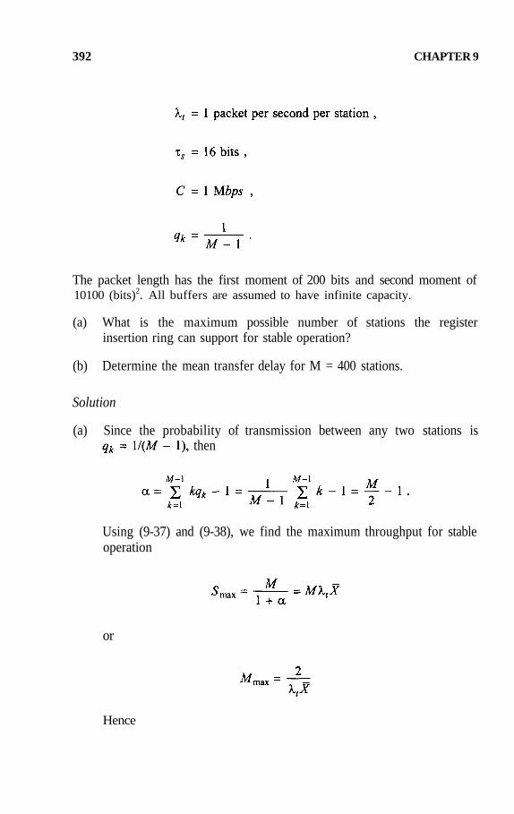
392 CHAPTER 9

The packet length has the first moment of 200 bits and second moment of10100 (bits)2. All buffers are assumed to have infinite capacity.

(a) What is the maximum possible number of stations the registerinsertion ring can support for stable operation?

(b) Determine the mean transfer delay for M = 400 stations.

Solution

(a) Since the probability of transmission between any two stations isthen

Using (9-37) and (9-38), we find the maximum throughput for stableoperation

or

Hence

CHAPTER 9 393

(b) The mean packet transmission time is

and the second moment of the packet transmission time is

For M = 400, we have

and

Using (9-38), we find the mean transfer delay

394 CHAPTER 9

9-10. SUMMARY

This chapter deals with the operation and performance analysis oflocal area networks with a ring geometry. Three types of ring networksare treated in detail: token rings, slotted rings, and register insertion rings.Depending on how the token is generated, operation of token rings can befurther classified into single token, multiple token, and single packetoperations. We derive expressions for the average transfer delay of allthree types of token rings.

For slotted rings the overhead must be taken into account. This isexpressed by the overhead factor. The actual operation of register insertionrings involves a number of queueing delays in series due to the tandemconnection of a number of station interfaces between the transmitting andthe receiving stations. A general model for such a connection requires atandem connection of queues for which an analytical treatment isintractable. Thus, we develop a simplified model and derive anapproximate expression for the average transfer delay.

Examples are given for illustration. Emphasis on modeling andanalysis has been made throughout the chapter. Using the simplified modelfor the analysis of register insertion rings, it is shown that the averagetransfer delay expressions for both the ring priority and station priorityschemes are the same.

REFERENCES


[2] Bertsekas, D. and Gallager, R., Data Networks, 2nd. ed., Englewood,Cliffs, N.J.: Prentice Hall, 1992.

[3] Penney, B.K. and Baghdadi, A.A., "Survey of ComputerCommunications Loop Networks: Part 1 and 2", ComputerCommunications, Vol. 2, 1979, pp. 165-180, pp. 224-241.

[4] Bux, W., "Local Area Subnetworks: A Performance Comparison",IEEE Trans. Communications, Vol. COM-29, No. 10, October 1981,pp. 1465-1473.

[5] Bux, W. and Schlatter, "An Approximate Method for thePerformance Analysis of Buffer Insertion Rings", IEEE Trans.Communications, Vol. COM-31, No. 1, January 1983, pp. 50-55.

CHAPTER 9 395

[6] Ferguson, M.J. and Aminetzah, Y., "Exact Results for Non-Symmetric Token Ring Systems", IEEE Trans. Communications, Vol.Com-33, No. 3, March 1985, pp. 223-231.

PROBLEMS

9-1. Consider the token ring network with 50 stations. Thecharacteristics of the network are as follows:

• Channel bit rate = 106 bps;

• Station latency = 1 bit;

• Length of ring = 5 km;

• Constant packet length = 75 bits;

• Average arrival rate per station = 50 packets per second; and

• Propagation delay = 5 per km.

Calculate the average transfer delay for (a) multiple tokenoperation, (b) single token operation, and (c) single packetoperation.

9-2. Consider the slotted ring network with the following features:

• Number of stations = 50;

• Channel bit rate = 5 Mbps;

• Length of ring = 1 km;

• Length of header = 24 bits;

• Number of slots in the ring = 4;

• Constant packet length = 2024 bits;

396 CHAPTER 9

• Station latency = 2 bits;

• Packet arrival rate to each station = 5 packets per second;and

• Propagation delay = 5

Calculate (a) the number of data bits in each slot, (b) the gaptime, and (c) the average transfer delay.

9-3. A token ring network has 100 stations and a channel capacityof 1 Mbps. Input traffic to each station is independent Poissonwith an average rate of 10 packets per second. All packets are500 bits long. The station latency is 2 bits and the propagationdelay for the complete ring is Calculate the averagetransfer delay for (a) multiple token operation, (b) single tokenoperation, and (c) single packet operation.

9-4. One hundred stations are connected to a local area ringnetwork with a channel bit rate of 10 Mbps. Each station hasa Poisson arrival process with an average rate of packets persecond. All packets are of 500 bits long. Propagation delayfor the complete ring is and the station latency is 2 bits.What is the largest possible value of for stable operation for(a) token ring, (b) slotted ring with unity overhead factor, and(c) register insertion ring with an average number of insertionbuffers traversed by a packet equal to fifty?

9-5. A token ring network 10 km long is to be designed to connectM stations. The connections are to be made with 96 Kbpslines. Each station serves 50 terminals, each of whichgenerates Poisson traffic with an average rate of 10 messagesper minute. Propagation delay is 5 Packets are of afixed length of 240 bits. The station latency is 2 bits.

(a) Express the average transfer delay in terms of M and plotthe result for multiple token operation.

(b) How many stations can be served if the average transferdelay is at most 0.1 second?

CHAPTER 9 397

9-6. A ring network has 100 stations to be connected with 1 Mbpslines. Each station generates Poisson traffic with an averagerate of 1 packet per second. The packet length is a constant of1000 bits. The propagation delay of the ring is 50Calculate the average transfer delay for (a) single tokenoperation with 2 bits station latency, (b) slotted ring networkwith an overhead factor equal to 1, and (c) register insertionring with equal probability of transmission to each of the otherstations.

9-7. A slotted ring network has 100 stations connected with 1 Mbpslines 20 km long. Each station has a latency of 2 bits. If theminipacket length must not exceed 50 bits, find two possibleminipacket lengths and keep the gap as small as possible.

9-8. A register insertion ring has 10 stations connected. Allstations have identical traffic characteristics. The traffictransmission pattern is as follows.

398 CHAPTER 9

Determine the maximum throughput.

CHAPTER 10

RANDOM ACCESS NETWORKS

10-1. INTRODUCTION

In Chapter 7, Section 7-5, we introduced the concept of randomaccess in the discussion of pure ALOHA and slotted ALOHA networks.Random access networks are characterized by the absence of a channelaccess control mechanism. The access technique used in the ALOHAnetwork is random in the sense that there is no predictable or scheduledtime for any station to access the communication channel that is shared byall of the stations attached to the network. When the network has a bus-type geometry, the signal received at one station depends on the signalstransmitted by all of the other stations. Typically, such a received signal isthe sum of the signals transmitted from all other stations. This type ofchannel (medium) is called a multi-access channel.

Conceptually, a multi-access communication system can be regardedas a queueing system. Each station has a queue of packets to betransmitted with the multi-access channel as a common server. Ideally, thecommon server should view all of the waiting packets as being in onecombined queue to be served by some appropriate queue discipline.Unfortunately, the server does not know which stations contain packets.Similarly, a station is unaware of packets at other stations.

In Chapter 7, we also obtained expressions for the throughput and theaverage transfer delay for both pure ALOHA and slotted ALOHAnetworks with Poisson input under steady-state conditions. However, thissteady-state assumption is often not justified, thus, the performance resultsobtained in Chapter 7 apply only for a short interval of time.

In this chapter, we shall investigate the effect of the throughput S, theoffered traffic G, and the backoff delay on the average transfer delay. Weshall show that the expression (7-27) is valid when the set of integers forthe backoff delay in a slotted ALOHA network approaches infinity; that is,when Furthermore, we shall obtain a more accurate expressionthan (7-27) for S in terms of G. We shall derive a Markovian model forthe slotted ALOHA network with a finite number of stations, and calculatethe state transition probabilities in Section 10-3. Using the determined

400 CHAPTER 10

stationary state probabilities, we shall calculate the throughput and theaverage transfer delay.

Section 10-4 presents the concept of equilibrium point forperformance analysis of slotted ALOHA. Section 10-5 explores thecarrier-sense multiple access (CSMA) protocols. Section 10-6 investigatesthe carrier-sense multiple access with collision detection (CSMA/CD)protocols, where the throughput analysis is based on the concept of a cycleconsisting of a busy period and an idle period.

10-2. PERFORMANCE ANALYSIS OF SLOTTED ALOHA WITHPOISSON INPUT

Recall that the slotted ALOHA procedure requires that the time axisbe divided into slots of fixed length P, which is the sum of the fixedpacket transmission time the processing time of the packet, and themaximum round-trip propagation delay. For local area networks, weassume that P equals and we neglect the processing time and thepropagation delay. Every transmitted packet must fit into one of these slotsby beginning and ending in precise synchronization with the slot.

For the slotted ALOHA operation after its arrival, a ready packet istransmitted at the beginning of the next slot. If the packet is successfullyreceived, then a positive acknowledgement is sent over a separate error-freechannel by the receiver. After a delay determined by the maximum two-way propagation time of the channel and the processing time in thereceiver, the sending station receives the acknowledgement. If a collisionoccurs, then no acknowledgement is sent. Thus, if the sending station doesnot receive an acknowledgement after a fixed time-out equal to the sum ofthe maximum two-way propagation time (quantized to slots) and theprocessing time in the receiver, the sending station selects a backoff timefor retransmitting the packet. A flow chart for the slotted ALOHAprotocol is given in Figure 10-1.

To obtain a more accurate expression than (7-30) for the averagetransfer delay, we first determine the average number of retransmissionsper successful transmission by defining the following conditionalprobabilities and :

CHAPTER 10 401

The probability of a successful transmission given that thetransmission is with a new packet; and

The probability of a successful transmission given that thetransmission is with a retransmitted packet.

We derive the following expressions for and in (10A-12) and (10A-13) respectively in Appendix A at the end of this chapter as:

402 CHAPTER 10

and

We also show in Appendix B that

In terms of and we can calculate the probability that a givensuccessfully transmitted packet requires exactly k retransmissions as

The average number of retransmissions can then be determined from pk

as follows:

Substitution of from (10-5) into (7-30) and neglecting and rP givesan expression for the average transfer delay

Thus, the normalized average transfer delay becomes

Furthermore, since G/S is the average number of transmissions persuccessful transmission, it follows from the definition of that

CHAPTER 10 403

Using (10-5) in (10-8) and solving for S gives

It is interesting to note that (10-6) and (10-9) are more accurateexpressions than (7-30) and (7-27), respectively. Moreover, using (10-3)as we see that both (10-6) and (10-9) reduce to (7-30) and (7-27),respectively.

The throughput S, as a function of G for several values of K, isplotted in Figure 10-2.

In the curves of Figure 10-2, note that the maximum throughput occurs atG = 1 for all values of K. The maximum throughput increases as Kincreases, reaching a peak value of as Most of the

404 CHAPTER 10

variation with K occurs for

Since the backoff delay is equivalent to the effective waiting time ina queue, the average number of packets in the backlog can be determinedby Little’s formula. Thus the average number of packets in the backlog isgiven by

We see from (10-7) that the normalized average transfer delay ofslotted ALOHA depends principally on the average retransmission delay ofthe packet. This fact has also been indicated by simulated studies.

Example 10-1. A slotted ALOHA network uses 1 Mbps lines toconnect 100 stations. Each station has a Poisson input with an average rateof 0.1 packets per second. Each packet is 1000 bits long. The propagationdelay and the collision detection time are negligible. The backoff algorithmrandomly selects an integer k with equal probability from the set of 10integers { 0,1,2, . . . 9 }. Under maximum throughput conditions, calculate(a) the average transfer delay using (7-30) and the more accurateexpression (10-6), and (b) the average number of backlogs for both cases.

Solution. Given data for the slotted ALOHA network are as follows:

Then

The average number of retransmissions is

(a) Neglecting the propagation delay and the collision detection time, weobtain from (7-30):

CHAPTER 10 405

Now, using (10-1) and (10-2), we find

and

Using (10-6), we obtain

(b) From (7-30), we find the average number of backlogs:

and the more accurate average number of backlogs is

10-3. PERFORMANCE ANALYSIS OF SLOTTED ALOHAWITH A FINITE NUMBER OF STATIONS

Because the slotted ALOHA system with Poisson input is alwaysunstable, the performance analysis in the last section cannot treat thestability problem. In this section, we formulate a Markovian model for theslotted ALOHA system and obtain the stationary state probabilitydistribution by calculating its state transition probabilities.

To develop a Markovian model for the slotted ALOHA system, wemake the following assumptions:

• There are M stations or users, with each user generating single-packetmessages;

• Each station is in one of two modes: the think mode and theretransmit mode. A station in the think mode is idle and has no

406 CHAPTER 10

packet for transmission. Thus it generates and transmits a new packetat the beginning of a time slot with probability A station is said tobe in the retransmit mode if it has a collided packet waiting forretransmission. A collided packet is transmitted in the current timeslot with probability p. A station in the retransmit mode cannotgenerate a new packet;

• The channel propagation delay is negligible or zero.

We adopt the zero channel propagation delay assumption here forsimplification of the modeling. However, the channel propagation delay isthe most important factor characterizing multiple-access broadcastcommunication in a distributed environment. In reality, we cannot ignorethe influence of the channel propagation delay in the modeling andanalysis. We shall discuss this problem again later. With the aboveassumptions, we depict a model for the system in Figure 10-3.

In the model, a station in either the think mode or the retransmitmode will enter the think mode in the next slot if its packet transmission issuccessful in the current slot. If the transmission is unsuccessful, it willenter the retransmit mode in the next slot.

CHAPTER 10 407

Now let be a random variable denoting the number of stationsin the retransmit mode at time t. The system is said to be in state k attime t if Thus, is a discrete-time Markov chain withthe discrete state space consisting of the set of integers {0, 1, 2, · · · , M}.Let the one-step state transition probabilities be

To calculate the state transition probabilities, we consider the followingcases:

(a) For , Since there can be only one successfultransmission in a time slot, the value of can decrease at mostby one.

(b) For the transition from state i to state j occurs when nonew packet is generated and a retransmitted packet is successful.Thus,

(c) For the transition from state i to state j occurs under twoconditions: (i) when there is only one new transmission and there isno retransmission, or (ii) when there are no new transmissions andzero or at least two retransmissions. Thus

(d) For the transition from state i to state j occurs when thereis one new transmission and at least one retransmission. Thus,

408 CHAPTER 10

(e) For the transition from state i to state j occurs when thereare new transmissions. Thus,

The stationary state probability distributionfor the Markov chain, where

can be computed by solving the following set of linear simultaneousequations:

and

Note that one of the equations in (10-12) is linearly dependent on theothers with the normalization condition (10-13).

10-3-1. Throughput Analysis. We shall now calculate thethroughput S that is defined as the average number of successfullytransmitted packets per transmission time of a packet. Denote by

the conditional throughput, given that From theformula of total probability, we calculate the mean throughput

CHAPTER 10 409

Since are known, it remains to determine the conditionalthroughput for all k. Given that is equal tothe conditional probability of exactly one (successful) packettransmission in a time slot. Thus, we have

Therefore, substitution of into (10-14) yields the meanthroughput S.

10-3-2. Average Transfer Delay. Since the average channel inputrate is

where

and

then, by applying Little’s formula to the model in Figure 10-3, weobtain

where

410 CHAPTER 10

The second term P on the right-hand side of (10-18) represents thefirst transmission time of the packet. Under steady-state conditions,

From (10-16) to (10-19), we finally obtain the average transfer delay

Dividing (10-20) by P yields the normalized average transfer delay:

As seen from the above analysis, the retransmission probability p isimplicitly contained in the expression for S and We can investigate theeffect of the values of p on the system performance by plotting thethroughput S and the normalized average transfer delay versus p forfixed values of M and A typical plot is shown in Figure 10-4 forM = 100 and

We see from Fig. 10-4 that as p increases to a certain threshold valueat about 0.043, the throughput decreases and the average transfer delayincreases very rapidly with p. This indicates that the system becomesunstable.

We have shown that the Markov chain model can be used to studythe dynamic behavior and the performance analysis of multiple accessprotocols. However, it is very difficult to extend the Markov chainmethods to more complicated protocols which are modeled as multi-dimensional Markov chains.

Example 10-2. In all of the analyses, we have assumed that theslotted ALOHA network is in statistical equilibrium. However, thisassumption is not always satisfied. The major factors in determiningstability of the slotted ALOHA are the number of stations M, the average

CHAPTER 10 411

backoff time and the average number of stations in the retransmissionmode,

For simplicity, suppose that and M is large, (a)Assume that the system is in state k; that is, there are k stations in theretransmit mode. Determine the probability that a given packet

412 CHAPTER 10

transmission is successful, and calculate the throughput (b)Determine the equilibrium point and the average transfer delay if thepacket length is 1000 bits long, stations, and the channeltransmission rate is 1 Mbps.

Solution. (a) Since the probability that a given packet transmission issuccessful equals the probability that no other packets are transmitted in thesame slot, then from (7-16) we obtain (when the system is in state k)

If the given packet is a new arrival, then

where and the approximations for small x,

and

have been used.

If the given packet is a backlogged packet, then

which has the same probability as the new arrival.

The throughput is equal to

(b) When the system is in state k, the throughput to the system is

CHAPTER 10 413

or

Now we write

or

At equilibrium,

We then have

Solving for G numerically, we find that

and

Since and we determine from (10-20) that

414 CHAPTER 10

It is interesting to note from (10-20) that if the number of stations Mincreases to infinity, there will be no finite average transfer delay.

When studying the infinite-station case, a multi-access system is oftendefined as being stable for a given arrival rate if the average transfer delayper packet is finite. In this sense, the ordinary slotted ALOHA with aPoisson input is unstable.

10-4. PERFORMANCE ANALYSIS OF SLOTTED ALOHA BYEQUILIBRIUM POINT

In order to analyze more complicated protocols in slotted ALOHA, ananalytical technique called the equilibrium point analysis may be used.The equilibrium point analysis assumes that the system is always at anequilibrium point. Therefore, the equilibrium point analysis does notinvolve the calculation of state transition probabilities.

Consider again the model in Figure 10-3. Let be a randomvariable (called the channel backlog) denoting the number of stations in theretransmit mode at time t. The channel input rate at time t is

Let [ S(t)] denote the channel state vector. From (10-15) and (10-17), we have

and

An equilibrium point is defined as a point at which the channel inputrate is equal to the channel output rate. By equating (10-23) and (10-24),we write

CHAPTER 10 415

Thus, the equilibrium point is a solution of (10-25). In solving thisequation, is assumed to be a real number in spite of the fact that thevariable k is an integer. If the number of solutions is one, then the systemis said to be stable. Otherwise, it is said to be unstable.

We plot and versus k in Figure 10-5, where anintersection of the straight line (the channel load line) representingand the curve for corresponds to an equilibrium point.

Figure 10-5(a) and Figure 10-5(b) represent a stable system becausethey have only one equilibrium point. The system corresponding to Figure10-5(c) is unstable. It is important to note that the system corresponding toFigure 10-5(b) is stable but overloaded. Therefore, by a stable system weusually mean the one in Figure 10-5(a) rather than Figure 10-5(b).

From (10-22), we see that (t)and S (t) are constrained to lie onthe channel load line (10-24). In Figure 10-5, arrows on the channel loadlines indicate directions of increasing backlog size k ifand decreasing backlog size k if As shown in Figure10-5(c), on an unstable equilibrium point such as the middle one, a smallperturbation will drift away from the equilibrium point. An unstablesystem always has two locally stable equilibrium points and one unstableequilibrium point. In that sense, an unstable system is also called abistable system. Generally, a stable system stays near the stableequilibrium point all the time and a bistable system goes back and forthbetween the two locally stable equilibrium points.

Note that the equilibrium point has two interesting properties.

(a) The steady-state throughput-delay performance of a stable system isclosely approximated by its stable equilibrium point;

(b) In an unstable system, the throughput-delay performance at a locallystable equilibrium point can be achieved only for some finite timeperiod.

In equilibrium point analysis, the throughput S is approximated bythe conditional expectation of the number of successful packettransmissions per packet transmission time given that the system is in state

416 CHAPTER 10

CHAPTER 10 417

k; that is,

Using we can calculate the average transfer delay. For example, inthe slotted ALOHA of Figure 10-3, we have from (10-21).

The Modified Model. When we apply the equilibrium point analysisto a Markovian model such as that of Figure 10-3, we often modify themodel in order to simplify the analysis. We modify the model in Figure10-3 by merging the two inputs to the slotted ALOHA channel into one.Since we usually assume bursty users, we consider the modification underthe condition We show the modified model in Figure 10-6, wherethe think mode in Figure 10-3 has been decomposed into two tandemphases, the think mode and the transmit mode, and where the retransmitmode in Figure 10-3 has become a part of the transmit mode in Figure 10-6.

A station which has just successfully transmitted a packet moves intoeither the think mode with probability or the transmit mode withprobability A station which has just had a collision enters thetransmit mode with a probability of 1. A station in the think mode willmove into the transmit mode at the next slot with probability and astation in the transmit mode transmits a packet (that is, moves out from thetransmit mode) with probability p. The modified model in Figure 10-6 isequivalent to the model in Figure 10-3 from the viewpoint of theprobabilistic behavior.

Now we let be a random variable denoting the number ofstations in the transmit mode at time t. Thus, is a Markov chain.From the modified model, the conditional throughput S ( k ) in state k isgiven by

418 CHAPTER 10

and

which has a simpler form than that of (10-15). Since

then by applying the procedure for obtaining the equilibrium point to themodified model, we have

CHAPTER 10 419

Solving this equation numerically for k under the condition that k is anonnegative real number yields an equilibrium point Thus, thethroughput S and the normalized average transfer delay can beexpressed as

and

respectively.

10-5. CARRIER-SENSE MULTIPLE ACCESS (CSMA)PROTOCOLS

For local area networks with stations located close together,propagation delays are usually much smaller than the packet transmissiontime. For such networks, it is feasible for a station that has a packet totransmit to listen to the channel to determine if it is busy before atransmission is attempted. If the channel is sensed busy, the station candefer its transmission until the channel becomes idle. This process iscalled carrier sensing. Networks with carrier sensing are called carrier-sense multiple access (CSMA) networks.

For satellite channels, carrier sensing is useless because thepropagation delays are much greater than the packet transmission time.For networks with propagation delays much shorter than the packettransmission time, CSMA-type protocols can have much smaller averagetransfer delays and higher throughput than the ALOHA protocols, since thecarrier sensing can reduce the number of collisions and the length ofcollision intervals.

The carrier sensing information can be used to reduce the number ofcollisions. There are several ways to make use of this information. Wemay divide CSMA protocols into two general classes: non-persistent andp-persistent. Operations for each of these classes can be slotted ornonslotted.

420 CHAPTER 10

For slotted operation, the time axis is divided into slots ofseconds, where is the end-to-end propagation delay of a bus or themaximum round-trip for a station on a broadband tree network. Like theslotted ALOHA, all stations for slotted CSMA operation must besynchronized and can start transmission only at the beginning of a slot.

Persistent and Nonpersistent CSMA Protocols. We describeCSMA protocols with the flow chart of Figure 10-7(a), which is anextension of that in Figure 10-1 to include a carrier-sense box. For slottedoperation, all time delays are quantized to slots of seconds.

Note that the flow chart of Figure 10-7(a) reduces to that of Figure10-1 for slotted ALOHA if the carrier-sense box is replaced by a directconnection. The CSMA protocols differ from the slotted ALOHA inhaving the decisions based on carrier sensing. If, at a certain instant, astation has a packet ready for transmission, the packet is called a readypacket and the station is called a ready station, irrespective of whether thepacket is a new or a retransmitted one.

Nonpersistent CSMA. With this protocol, collisions are reducedbecause a station that finds the channel busy always defers thetransmission. When a station becomes ready, it senses the channel andcarries out the following procedure:

1. If the station senses that the channel is idle, it transmits the packet;

2. If the channel is sensed busy, the station uses the backoff algorithmto reschedule the packet to a later time. After then, the station sensesthe channel again, and the procedure is repeated.

Persistent CSMA. Persistent CSMA protocols have two differentversions: 1-persistent CSMA and p-persistent CSMA. The 1-persistentCSMA never allows the channel to go unused when there is a readystation. The operation is as follows. A ready station senses the channeland then carries out the following procedure:

1. If the station senses that the channel is idle, it transmits the packet;

2. If the station senses the channel to be busy, it keeps on sensing thechannel until the channel becomes idle and then transmits the packet.

CHAPTER 10 421

422 CHAPTER 10

When two or more ready stations sense the channel to be busy, with1-persistent CSMA they all wait until the channel becomes idle and thentransmit. In this case, a collision must occur (with probability 1). If wereduce this probability to p, 0 < p < 1, the chance of a collision isreduced.

For p-persistent operation, a ready station after sensing the channel,operates as follows:

1. If the channel is sensed idle, then the station transmits the packetwith probability p, or the station waits seconds with probability1-p, and the procedure is repeated;

2. If the channel is sensed busy, then the station keeps sensing thechannel until it becomes idle, and then it operates as in step 1.

10-5-1. Throughput Analysis of Non-persistent CSMA. To give anapproximate throughput analysis of nonpersistent CSMA, we make thefollowing assumptions:

• The arrival process (both new and collided packets) is Poisson with arate of packets per second;

• The propagation delay between any two stations on the bus isseconds, which is the maximum one-way propagation;

• At any time, each station has at most one packet ready fortransmission;

• Carrier sensing is instantaneous and the turn-around time in switchingfrom transmitting to receiving is zero;

• The channel is error-free so that failure of transmission is due tocollision only;

• The overlap of any fraction of two packets results in retransmissionof both packets.

Let be the offered traffic and S be the throughput, which isdefined as the number of successful transmissions per packet transmissiontime. A model of the system is shown in Figure 10-8.

CHAPTER 10 423

Suppose that at time t, the channel is idle and packet 0 arrives asshown in Figure 10-9. This packet is transmitted immediately with atransmission time of P seconds. Since the propagation time is theother stations do not sense packet 0 before time If these stationshave arrivals in the time interval [ t, ), they transmit the packetsimmediately. Packet n is the last packet that arrives at a random time Y in[ t, ). After time all stations have sensed the channel to bebusy. According to the nonpersistent CSMA protocols, further arrivals suchas packet n + 1 will be rescheduled for transmission at a later time.Transmission of packet n is completed at time t + Y + P. All stationssense the end of packet n at time t + Y + P + but up to this time, allarrivals after packet n are rescheduled for transmission at a later time.

After time t + Y + P + , all stations sense the channel to be idle.The next transmission at t1 initiates another cycle. The intervals[ t, ) and [ , t1) are called a busy periodand an idle period, respectively. A cycle consists of a busy period and anidle period.

The busy period shown in Figure 10-9 is an unsuccessful busy periodbecause there are more than one arrival in [ t, ). On the other

424 CHAPTER 10

hand, if packet 0 is the only arrival in [ t, ), then the busy period isa successful busy period.

From this observation, we see that the vulnerable period for CSMAprotocols is the maximum one-way propagation delay This is animprovement when compared with vulnerable periods of P and 2P for the

CHAPTER 10 425

slotted ALOHA and the pure ALOHA, respectively, provided that

Using the notion of busy-idle period (or cycle) just described, we cancalculate the throughput for the non-persistent CSMA channel. Let Vdenote the length of time for successful transmissions in a cycle, and letdenote its average value. Since the average length of a cycle is +where and are the average values of the busy period and the idleperiod, respectively, the throughput can be expressed as

This expression follows from the fact that under steady-state conditions, thethroughput (the average number of successful transmissions) S is equal tothe ratio of the average time for transmitting successful packets to theaverage cycle time. It remains to find and

Since the average time for successful transmissions in a cycle equalsthe product of the probability of successful transmissions and the packettransmission time, we write

Furthermore, since packet arrivals are Poisson with an average rate of G/Ppackets per second, and since the probability that packet 0 is successfullytransmitted is equal to the probability that there are no other arrivals in[t, ), we have

and hence

Referring to Figure 10-9, note that the busy period B has the length

426 CHAPTER 10

where Y is a random variable. It is not necessary to differentiate betweena successful and unsuccessful transmission or collision in (10-36) becausethe busy period B here includes successful transmissions as a special case;that is, Y = 0. Thus,

To find the distribution function of Y , we note that t + Y is the lastpacket arrival time in [t, ), so that is the probability ofno arrivals in [ y, ). Thus,

This distribution function has a jump of size at y = 0.

The average value of Y is given by

and from (10-37), the average busy period is

To compute the average idle period we recall that a Poisson arrivalprocess with mean rate G/P and an exponential interarrival time withmean P/G are equivalent. The idle period is simply the time intervalbetween the end of a busy period and the next arrival epoch. Because ofthe Markov property (or memoryless property) of the exponentialinterarrival time, the average idle period and the mean interarrival time are

CHAPTER 10 427

equal. Thus,

Substituting , and into (10-32) yields

or

where

In particular, if or then

From (10-43), we see that as a becomes small, S approaches this limitingvalue.

Curves showing the relationship between S and G from (10-43) aregiven in Figure 10-10 for several values of α.

428 CHAPTER 10

10-5-2. Throughput Analysis of Slotted Non-persistent CSMA. For anapproximate analysis of the slotted nonpersistent CSMA, in addition to theassumptions for the non-persistent CSMA, we assume that the time axis isdivided into slots of equal length A diagram for the slotted non-persistent CSMA, similar to Figure 10-9, is shown in Figure 10-11.

Suppose that the channel is idle at time 0 and there is at least onearrival in the first slot. Packet 0 is transmitted at time 1. If this is theonly packet arrival in the first slot, then it is a successful transmission.Otherwise, the transmission is unsuccessful. In either case, the busy periodis exactly seconds.

We shall compute S in terms of , and using (10-32). First,consider the events occurring in the first slot (0, ) and their associatedprobabilities. Note that

CHAPTER 10 429

430 CHAPTER 10

Thus, using (10-33), we obtain

From Figure 10-11, we see that the busy period is a deterministic quantity:

In the slotted case, the average idle period can be written as

where is the average number of slots in an idle period. Since thearrival process is Poisson and arrivals in disjoint slots are mutuallyindependent, we can write

and

In general, we obtain

Therefore, the mean value of is

CHAPTER 10 431

Using (10-49), (10-50), and (10-53), we obtain

Finally, substituting expressions (10-47), (10-48), and (10-54) for , andrespectively in (10-32), we obtain

Graphs of S versus G for several values of a are plotted in Figure 10-12.

432 CHAPTER 10

10-6. CARRIER-SENSE MULTIPLE ACCESS WITH COLLISIONDETECTION (CSMA/CD) PROTOCOLS

A further improvement on the carrier-sense multiple access protocolscan be obtained by using collision detection. Collision detection, alsocalled "listen while transmit", means to detect a collision shortly after itoccurs. Thus, unsuccessful transmissions can be aborted promptly,minimizing the length of unsuccessful periods.

To implement the collision detection, the transceiver must monitor thechannel before transmitting and also while transmitting. Like the CSMAprotocols, the CSMA/CD protocols can have variations such as slotted andunslotted, and non-persistent and p-persistent. For all of these variations,the use of collision detection provides improved performances for localarea networks with a short bus such that the normalized propagation delayis small. If a local area network does not have a small normalizedpropagation delay, CSMA/CD is not always the logical choice.Nevertheless, CSMA/CD is perhaps the most commonly used randomaccess protocol for local area networks.

Basic Operation. The basic operation of the CSMA/CD can bedescribed by the flow chart in Figure 10-13.

As shown in the diagram, the operation of CSMA/CD is the same asfor CSMA before the collision detection box. After the packet istransmitted, CSMA/CD is capable of "listen while transmit". If nocollision is detected, the transmission is successful. On the other hand, if acollision is detected, the transmission is promptly aborted, a jammingsignal is sent, and the collided packet is backed off in the same manner asfor CSMA.

We can describe the variation of CSMA/CD for a ready station asfollows.

1. If the channel is sensed idle:

• for the nonpersistent and 1-persistent CSMA/CD, the packet istransmitted;

• for p-persistent CSMA/CD, the packet is transmitted with probabilityp, and is delayed by seconds with probability 1 – p;

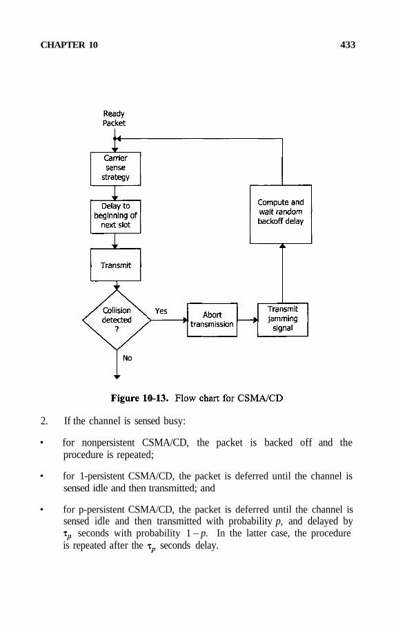
CHAPTER 10 433

2. If the channel is sensed busy:

• for nonpersistent CSMA/CD, the packet is backed off and theprocedure is repeated;

• for 1-persistent CSMA/CD, the packet is deferred until the channel issensed idle and then transmitted; and

• for p-persistent CSMA/CD, the packet is deferred until the channel issensed idle and then transmitted with probability p, and delayed by

seconds with probability 1 – p. In the latter case, the procedureis repeated after the seconds delay.

434 CHAPTER 10

3. If a collision is detected while transmitting, the transmission isaborted and a jamming signal is sent, and all stations involved in acollision backoff; and

4. After the packet backs off, the procedure is repeated.

The jamming signal is not an essential feature of CSMA/CD.However, it is commonly used by local area networks such as Ethernet.The jamming signal is used to ensure that all other stations know of thecollision and backoff. Commercial local area networks often use the 1-persistent CSMA/CD protocol with a backoff algorithm. For example,Ethernet uses the truncated binary exponential type backoff algorithm. Oneversion of this algorithm allows only 16 attempted transmissions. Afterthen, the packet is discarded. For each retransmission, the backoff time is

where r is an integer selected from the set of integers(0, 1, • • • , ) with ( 10, number of attemptedtransmissions to date). In this case, the backoff time changes with thenumber of collisions. Thus, the backoff strategy is a dynamic one.Dynamic backoff strategy is sometimes called a linear incremental backoffstrategy because the mean backoff time is linearly proportional to thenumber of collisions experienced by a given packet.

To illustrate the detailed operation of the CSMA/CD using jamming,consider the two-dimensional diagram in Figure 10-14. Suppose that attime 0, station A begins transmission. Since other stations will not detectthe transmission until after the propagation delay of seconds, CSMA/CDhas a vulnerable period of seconds. For most analyses, is taken tobe the maximum end-to-end propagation delay of the channel. If twospecific stations are considered as in Figure 10-14, is denoted byA station requires seconds to detect a collision.

Now consider that before the signal from station A arrives at stationB, station B initiates a transmission at time Y, where Y is a randomvariable. Shortly after the transmission of station B, the signal from stationA arrives, and seconds later, station B detects the collision and thensends out a jamming signal for J seconds. The jamming signal from stationB reaches station A at time Station A then sends out ajamming signal for J seconds. Station B will receive the completejamming signal at time During this period, the channelis always busy. After time the channel becomes idle.

CHAPTER 10 435

We can define busy period and idle period for the CSMA/CD channelin the same manner as for the CSMA channel. An idle period is a timeinterval during which the channel is not used by any station. A busyperiod is an unsuccessful busy (collision) period if more than one stationtransmits in the period. A busy period is a successful busy period if onlyone station transmits in the period. In Figure 10-14, the busy period[0, ] is an unsuccessful busy period.

436 CHAPTER 10

Example 10-3. Consider the transmission of two stations on aCSMA/CD network. Suppose that the backoff algorithm used is the binaryexponential algorithm, where the propagation delay between the collidingstations is neglected. Find

(a) The probability that the first retransmission is unsuccessful;

(b) The probability that the second retransmission is unsuccessful, andthe probability that the nth retransmission is unsuccessful; and

(c) The probability that the first successful transmission occurs on the nthretransmission.

The binary exponential backoff algorithm is described as follows:

After k collisions, the kth retransmission of each colliding station isdelayed by an amount equal to an integer r times the base backoff time.The integer r is selected with equal probability from the set of integers{ 0, 1, . . . , }. The base backoff time is often chosen twice theend-to-end propagation time.

Solution. (a) After the first collision, k=l, each colliding stationselects an integer r from the set {0,1} with equal probability. Let

denote the outcomes for the two stations. Since each station hastwo choices, there are four possible outcomes: (0,0), (0,1), (1,0), (1,1).The first retransmission will collide again for either (0,0) or (1,1). Thus,the probability that the first retransmission is unsuccessful is

(b) after two collisions, k = 2, the set of integers for selecting r is {0, 1, 2,3}. The number of possible outcomes for the two stations is

all are equally likely. A collision will occur again foroutcomes (0,0), (1,1) (2,2) or (3,3). Thus,

In general, for k = n, the set of integers for selecting r is {0, 1, . . . ,which has integers in total. There are possible choices

CHAPTER 10 437

of

of which cause another collision; that is,

(0,0) , (1,1) ,. . . ,

Thus, we obtain

(c) In order that the first successful transmission occurs on the nthretransmission, the first (n-1) retransmissions must result in collisions, andthe nth retransmission (or equivalently the (n+l)th attempt) must be asuccessful transmission. Thus, we have

P { First successful transmission on the nth retransmission }

= P { Collision on each of first (n-1) retransmissions and no collisionon the nth retransmission }

{ Collision on the kth retransmission } × P { no collision on

the nth retransmission }

Throughput Analysis for Non-persistent CSMA/CD. To give athroughput analysis for non-persistent CSMA/CD, we make the followingassumptions in addition to those given in Section 10-5:

• The time required to detect a collision is negligible; and

• The jamming time J is the same for all stations.

We use the same approach in (10-32) to calculate the throughput S interms of , and Consider first the average busy period Since abusy period can be either a successful transmission period with probability

438 CHAPTER 10

and length , or a collision period (unsuccessful period) withprobability and average length , we write

where is the probability of a successful transmission, and C is thelength of a contention period. Note that is equal to the probability ofhaving no arrivals in the vulnerable period [0, ). Thus,

It remains to compute the average length of a collision period . Tosimplify the calculation, we let be the propagation delay between everypair of stations. This assumption implies that all adjacent stations areequally spaced. Figure 10-15 shows three colliding transmissions.

In the figure, suppose that station 1 begins a transmission at time 0,while stations 2 and 3 begin transmission at times X and Y respectively,with X being less than Y. Observe that the instant at which the firstpacket collides with the packet of station 1 determines the length of thecollision period C. Thus,

and

To compute the distribution function of X, it is useful to think of Xas the first arrival time in [0, ), given that there is at least one arrival inthis interval. Thus, is the conditional probability of no arrivalsin [0, x), given that at least one arrival occurs in [0, ). We can write

CHAPTER 10 439

by using the fact that Poisson arrivals in nonoverlaped time intervals areindependent.

The average value of is given by

440 CHAPTER 10

Using (10-59) and (10-61), can be expressed as

From (10-56), (10-57) and (10-62), we obtain

The average time of a successful transmission is given by

The average idle period is the same as that of (10-41):

Using these results in (10-32) yields

Throughput Analysis for Slotted Non-persistent CSMA/CD. Forslotted non-persistent CSMA/CD, the throughput analysis is closely parallelto that for the slotted non-persistent CSMA presented in Section 10-5.

From (10-47), we have the average length of time for a successfultransmission:

CHAPTER 10 441

Since the length of the idle period does not depend on whether or not theCSMA protocol has collision detection, we obtain from (10-54)

To compute using (10-56), we require the probability of asuccessful transmission in (10-46),

We also need the average length of the collision period . Consider twostations, both transmitting a packet at time 0 ( at the beginning of a slot).These transmissions certainly lead to a collision. Of course, is the slottime equal to the end-to-end propagation delay. For slotted operation, thejamming time J is also an integral number of slots. Figure 10-16 showssuch a collision period for slotted CSMA/CD.

Examination of the figure indicates that the collision period has aconstant length of Thus, the average length of the collisionperiod is

and from (10-56), (10-69) and (10-70), we find the average length of thebusy period:

442 CHAPTER 10

Using the results for and in (10-32) yields

where

It is interesting to note that if

then

CHAPTER 10 443

Introducing for in (10-72) yields

which is identical to the throughput in (10-55) for slotted non-persistentCSMA.

Note that the throughput for non-persistent CSMA/CD does notreduce to the result for non-persistent CSMA. This is because the lengthof the collision period for CSMA/CD depends on the arrival time of thefirst colliding packet, while that for CSMA depends on the last collidingpacket.

10-7. SUMMARY

This chapter deals with random access networks, which do not have achannel access control mechanism for controlling when a station cantransmit. The basic random access method was discussed in Section 7-5for using the pure ALOHA network with Poisson input. The chapterbegins with the slotted ALOHA with Poisson input. Unlike the pureALOHA, the slotted ALOHA allows packets to be transmitted only at thebeginning of the next slot after arrival. With this restriction, the slottedALOHA method is not a completely random access method in the strictestsense; it also requires that all stations maintain slot synchronization. Adrawback of the slotted ALOHA system with Possion input is that thesystem is always unstable.

For stability considerations, the chapter treats a slotted ALOHAsystem with a finite number of stations. Generally, the throughput as wellas the average transfer delay depends on the retransmission probability.Instability can occur when the retransmission probability exceeds a certainthreshold value. By assuming the existence of an equilibrium point in thesystem, it is possible to apply the Markov chain method for stabilityconsiderations and performance analysis.

444 CHAPTER 10

If hardware at each station is available for listening to the channeland determining whether the channel is free before transmission, thencarrier-sense methods can be employed. These methods are carrier-sensemultiple access (CSMA) and carrier-sense multiple access with collisiondetection (CSMA/CD). Both methods can be further classified intononpersistent and p-persistent, and slotted and nonslotted. By means ofCSMA or CSMA/CD, the maximum throughput can be increased.

By adding still another handware feature of monitoring the channelbefore transmitting and also while transmitting to a station, furtherimprovement in maximum throughput over the CSMA is possible.Generally speaking, CSMA/CD performs better than CSMA. Applicationof both CSMA and CSMA/CD requires that the normalized propagationdelay over the channel be small. Small normalized propagation delays aretypical for local area networks. Thus, significant improvements inmaximum throughput can be obtained.

REFERENCES

[1] Lam, S.S., "Packet Switching in a Multiple-Access BroadcastChannel with Application to Satellite Communications in a ComputerNetwork", Ph.D. dissertation, Computer Science Department,University of California, Los Angeles, March 1974.

[2] Kleinrock, L., Queueing Systems, Vol. 2, Computer Applications,New York: John Wiley & Sons, 1976.

[3] Kleinrock, L. and Lam, S.S., "Packet Switching in a MultiaccessBroadcast Channel: Performance Evaluation", IEEE Trans.Communications, Vol. COM-23, No. 4, April 1975, pp. 410-423.

[4] Lam, S.S. and Kleinrock, L., "Packet Switching in a MultiaccessBroadcast Channel: Dynamic Control Procedures", IEEE Trans.Communications, Vol. COM-23, No. 9, September 1975, pp. 891-904.

[5] Lam, S.S. and Tobagi, F.A., "Packet Switching in Radio Channels:Part I - Carrier Sense Multiple Access Methods and Their Throughput- Delay Characteristics", IEEE Trans. Communications, Vol. COM-23, No. 12, December 1975, pp. 1400-1416.

CHAPTER 10 445

[6] Tobagi, F.A. and Kleinrock, L., "Packet Switching in RadioChannels: Part IV - Stability Considerations and Dynamic Control inCarrier Sense Multiple Access", IEEE Trans. Communications, Vol.COM-25, No. 10, October 1977, pp. 1103-1119.


[8] Tobagi, F.A. and Hunt, V.B., "Performance Analysis of Carrier SenseMultiple Access with Collison Detection", Computer Networks, Vol.4, 1980, pp. 245-259.

[9] Tasaka, S., Performance Analysis of Multiple Access Protocols,Cambridge, Mass.: MIT Press, 1986.

[10] Massey, J.L., "Some New Approaches to Random-AccessCommunications", in Multiple Access Communications, ed.Abramson, N., Pitscataway, Mass.: IEEE, 1993.

[11] Capetanakis, J.I., Tree Algorithms for Packet Broadcast Channels",IEEE Trans. Inform. Theory, Vol. IT-25, No. 5, September 1979, pp.505-515.

[12] Tsybakov, B.S. and Bakirov, V.L., "Packet Transmission in RadioNetworks", in Multiple Access Communications, ed. Abramson, N.,Piscataway, Mass.: IEEE, 1993.

[13] Bertsekas, D. and Gallager, R., Data Networks, 2nd ed., EnglewoodCliff, N.J.: Prentice Hall, 1992.

PROBLEMS

10-1. A slotted ALOHA multi-access channel connects M nodes.Assume that when a node is in the transmit mode, it can accept apacket with probability σ , and when in the retransmit mode, itcannot accept a packet. The slot size is one time unit. Let

the number of nodes in the retransmit mode at thebeginning of the kth slot; and

where

446 CHAPTER 10

Note that depends on the particular manner in which collisionsare resolved, but we assume that is given here.

(a) Find the average number of accepted arrivals per slot as afunction of NR, M, and

(b) Find the average number of packets in the system which isthe average number of backlogs plus the average number of newarrivals during the previous slot.

(c) Obtain an expression for the average transfer delay T.

10-2. Assume, for simplicity, that each transmitted packet in a slottedALOHA system is successful with some fixed probability Newpackets are assumed to arrive at the beginning of a slot and aretransmitted immediately. If a packet transmission is unsuccessful,it is retransmitted with probability p in each successive slot untilsuccessfully transmitted.

(a) Find the normalized average transfer delay

(b) Suppose that the number of nodes M is large, and that and pare small. Show that in state k, the probability γ that a givenpacket transmission is successful is approximately equal towhere and and p are defined inSection 10-3.

10-3. An approximate expression between S and G for slotted ALOHAnetworks is

(a) Determine an expression for the average transfer delay persuccessful packet transmission in terms of G, P, and Thebackoff algorithm is the binary exponential backoff that is used inEthernet. This backoff algorithm can be described as follows: Ifa packet has been transmitted unsuccessfully k times, then theprobability of transmission in successive slots isWhen a packet initially arrives at a station, it is transmittedimmediately in the next slot.

(b) Suppose that the network has the following parameter values:

CHAPTER 10 447

• Channel bit rate = 1 Mbps;

• Average packet length = 1000 bits;

•

• The detection delay for determining whether or not a transmissionis successful is negligible.

Determine the average transfer delay in slots or packet times.

10-4. A slotted ALOHA network has M stations, each with an infinitelylarge buffer and a Poisson arrival of average rate packets persecond. New arrivals are considered as backlogs immediatelyrather than transmitted in the next slot. When a station containsone or more packets, it independently transmits one packet in eachslot with probability p. Assume that any given transmission issuccessful with probability

(a) Show that the average time from the beginning of a backloggedslot until the completion of the first successful transmission at a

given station is and the second moment of this time is

(b) Note that the assumption of a constant probability for a successfultransmission allows each station to be considered independently.Use the service time results of part (a) to show that the averagetransfer delay is

(c) Assume that (this assumption corresponds to very lightloading and yields a smaller T than any other value of

Calculate T for and compare it with the average transfer

delay for TDMA if M is large.

448 CHAPTER 10

10-5. A group of personal computers uses a pure ALOHA accessscheme to communicate over a bus network. All packets are 50bytes long and the channel bit rate is 120 Kbps. If each computergenerates 10 packets per minute on average, how many computerscan the network support?

10-6. Consider the transmission of two stations on an Ethernet that usesCSMA/CD (carrier sensing multiple access with collisiondetection) and a truncated binary exponential type of backoffalgorithm which allows an initial attempt plus 15 retransmissions,each delayed by an integer r times the base backoff time. Theinterger r is selected randomly from a set of integers {0,1, . . . ,2k–1}, where { number of retransmissions to date, 10}.After 16 attempts, the packet is discarded. Find the probabilitythat a packet is discarded, and determine the average number ofretransmissions per packet.

10-7. A slotted CSMA/CD network has M stations operating with slotsof identical length equal to twice the end-to-end propagation delay;that is, Under heavy load conditions, assume that eachstation always has a packet in queue. The probability of a stationinitiating a transmission in a slot (at the beginning of the slotboundary) is

(a) Calculate the probability of some station having a successfultransmission in a given slot. What value of σ maximizes ?

(b) What is the average number of slots wasted before some stationhas a successful transmission? Express the average contentiontime in terms of M, and

(c) Let P be the transmission time of a successful packet. Derive anexpression for the throughput S in terms of P, , M, and ,where Show that S is maximized with respect to bythe same maximized value as in part (a). Find an expressionfor the maximum throughput.

(d) For a channel bit rate of 3 Mbps, packets of length 1024 bits, andpropagation delay of 8 , calculate the maximum throughputwhen M = 4, 64, and 256. What limit does the maximumthroughput approach as M tends to infinity?

CHAPTER 10 449

APPENDIX A - Determination of qn and qr

Equation (10-5) expresses the average number of retransmissionsin terms of the probabilities and of (10-1) and (10-2), respectively.

To derive and , we first recall that after transmission of apacket, a station must wait slots to determine if the transmission issuccessful or has collided. Consider the event of a successful transmissionwhich takes place in the current slot, labelled slot C in Figure A-1. If thesuccessfully transmitted packet in slot C is a retransmitted packet, it musthave had a collision in an earlier slot, such as slot A. Thus, the collisionmust have taken place in one of the K earlier slots such that the currentslot is (r + k) slots after the transmission of the collided packet, where

and k is chosen at random from the set of integers, {0, 1, 2,..., K- 1}.

For the retransmission to be successful, all of the following threeevents must occur:

1. No new packets are generated in slot C;

2. No other packets that collided in slot A are retransmitted in slot C;and

450 CHAPTER 10

3. No packets that collided in one of the other K-l slots, other than slotA, are rescheduled for slot C.

Assume that the above three events are independent. Let

Using these probabilities, we have

If the packet that is successfully transmitted in slot C is a new packet,two independent events must take place:

(a) No other new packets are generated in slot C; and

(b) No retransmissions occur in slot C from collisions in any earlier slots.

It follows that

It now remains to determine the probabilities forSince the arrival process of new packets is Poisson with a rate of packetsper slot and there are M stations, we have

To determine we let q(j) be the probability that, in addition to thepacket successfully transmitted in slot C, exactly j other packets aretransmitted in slot A and none of these packets is retransmitted in slot C.Since the packet arrival process (new plus retransmitted) is Poisson withrate A, the probability of exactly j arrivals in slot A is given by

where

CHAPTER 10 451

Furthermore, the probability of not transmitting a collided packet in slot Cis the probability of not choosing one value of the back off integer k,which results in retransmission in slot C. This probability is equal to

Assuming all events are independent, q(j) can be expressed as

Let us define the following two events:

X = In addition to the successfully transmitted packet in slot C, atleast one other packet is transmitted in slot A and none of thesepackets is transmitted in slot C,

and

Y = A collision occurs in slot A (or at least one other packet is generatedin slot A).

Then we have

Since the packet arrival process is Poisson with rate then

The probability is the probability Therefore,

Substituting (10A-5) into (10A-8) yields

452 CHAPTER 10

To calculate we consider the event that no retransmissions fromcollisions in a slot other than slot A (for example, slot B) occur in slot C.This event can occur in one of three mutually exclusive ways:

(a) No arrivals and hence no transmission occurs in slot B;

(b) One arrival and hence a successful transmission occurs in slot B sothat no retransmission is needed in slot C; and

(c) Two or more transmissions take place in slot B, but none isretransmitted in slot C.

The probabilities of the first two events are determined by thePoisson arrival process to be and , respectively. The last eventis the union of the events with probability q(j) for j from 2 to . Thus,the probability of the last event is

Since is the probability of the union of the above three mutuallyexclusive events, we finally obtain

Substituting q1, q2, and q3 into (10A-1) and (10A-2) yields the results in(10-1) and (10-2), respectively, as

CHAPTER 10 453

and

APPENDIX B - Determination of the limiting values of and

From (10-9) and (10A-1) to (10A-3), we have

where

Since G is a constant, , and

then

It follows that

454 CHAPTER 10

We now proceed to find this common limit, which we denote by ,

Since S is also a constant,

Note that as

where

We need to calculate

Thus, we obtain

A solution to this functional equation is

CHAPTER 10 455

To show that is the unique solution, we assume that is anothersolution.

If , then . Thus,

which is a contradiction.

If , then Hence,

which leads to a similar contradiction.

Therefore, we conclude that is the unique solution.

ANSWERS TO SELECTED PROBLEMS

Chapter 1

1-4 4.9

1-5 (a) 20.83, (b) 20.41, (c) 0.82

Chapter 2

2-6 4.56 mH/km

2-8 7 km

2-9 4.6 km

Chapter 3

3-1 3 × 3; 52,488

3-2 52,488

3-5 0.02

Answers to Selected Problems 457

Chapter 4

4-1 (a) 0.96 seconds, (b) 1.79 seconds

4-2 (a) 0.6, (b) 3.6 min.

4-3 (a) 0.4, (b) 1.33 min., (c) 6.9 min., (d) 1.8

4-4 (a) 110, (b) 0.3, (c) 0.06 seconds, (d) 0.42

4-5 (a) 300, (b) 0.12s

4-6 (a) 710 packets/sec., (b) 0.64 ms

4-7 (a) 163 packets/sec., (b) 0.025 sec., (c) 3.12, (d) 0.019s, (e) 0.88

.(b)

4-10 (a) 0.78, (b) 0.14

4-12 (a) 909 packets/sec., (b) 0.909 erlangs

(b) 0.51s, (c) 10.2

4-14 (a) 0.1, (b) 1.6ms

(b)

458 Answers to Selected Problems

4-16 (a) 40, (b) 0.9, (c) 0.3 s, (d) 0.6

(b)

4-18 (a) 1.63, (b) 7.09 s

4-19 (a) 0.67, (b) 1.33, (c) 2

(b) , (c)

4-21 (a) 100, (b) 0.4 s

(b)

(b)

4-29 (i) (a) 0.5665, (b) 1.087, (c) 0.217 s

(ii) (a) 0.565, (b) 1.085, (c) 0.0217 s


Chapter 5

5-1 (a) 22, (b) 21, (c) 0.015

5-2 (a) 0.0267, (b) 0.02

5-3 0.75

5-4 (a) 1000 ccs, (b) 0.1 ccs per subscriber, (c) 0.0028, (d) 0.01, (e)0.72

(c)

5-8 (a) 0.03; 3,

(b) 0.09; 2.7s; 3; 0.4s

5-9 (a) 44.37, (b) 0.27, (c) 44.73

5-10 (a) 8.29, (b) 13

5-11 (a) 1/3, 1/3, 1/3, (b) 6.67, (c) 8

5-13 (a) 0.025, (b) 0.02, (c) 0.11 min; 0.95 min

5-15 (a) 0.154; 0.4201, (b) 2.73, (c) 15.12; 22.27, (d) 2

5-16 (a) 9.63; 7.704; 0.8, (b) 0.37; 0.8134; 1.2

Chapter 6

6-1 (a) 15, (b) 10

6-2 (a) 0.0131, (b) 0.0066, (c) 0.013

6-3 (a) 0.0236, (b) 0.1816, (c) 2.38 s, (d) 0.0213

460 Answers to Selected Problems

Chapter 7

7-1 (a) 40, (b) 0.1

7-2 0.8; 0.94

7-3 81.8; 86.72

7-4 (a) 58.33 ms, (b) 33.43 ms

7-5 (a) 50, (b) 93

7-6 (a) 1.33 ms, (b) 0.33 ms

7-8 (a) 1 - y, where y is the overhead factor, (b) 1.98%

7-9 (a) 0.24, (b) 1.4 packets/s, (c) 0.6, (d) 7.3 ms

7-10 (b) 0.4862

Chapter 8

8-1 (a) 93, (b) 3571

8-2 (a) 1667 bps, (b) 4.26 s; 4.32 s; 4.3 s, (c) 7.66 s

8-3 1200 bps

8-4 (a) 52, (c) 80

Chapter 9

(b) , (c)

, (b) , (c)

9-3 (a) 1.06 ms, (b) 1.06 ms, (c) 1.4 ms

9-4 (a) 142 packets/s, (b) 1000 packets/s, (c) 392 packets/s


9-5 (b) 50

9-6 (a) 1.32 ms, (b) 2.38 ms, (c) 24.16 ms

9-7 50 bits; 30 bits

9-8 2.41

Chapter 10

(b) (c)

(b)

10-3 (b) 2.42 ms

10-5 331

(d) 0.9255

INDEX

AC loss limit 41Accessibility 224, 233Addition rule of probability 202Alerting 70ALOHA

pure 318-321, 399,425with caputres 324slotted 325-400, 403-406, 411slotted with captures 331vulnearable period 320, 326-327

Alternate routing network 16, 236, 263-267

American Telephone andTelegraph in the United States (AT& T) 15-19,31

American wire gauge 42-43Apparent offered load adjustment factor

369ARPAnet 1, 11-12, 28Arrival epoch 121Arrival process 155Arriving customer’s distribution 159,

247, 287-300Artificial delay 378Asynchronous time-division

network (ATDM) 2,54Asynchronous transfer mode

(ATM) 1-2, 31Attending 70Attenuation 37, 41, 50-51, 62-63Attentuation limit 41,44-45, 48Average, mean, expected value

arrival rate 25busy hour traffic 27interarrival time 15queue length 156, 173-174service time 25system time 161transfer delay 308weekday traffic 27waiting time 156, 174, 190, 242-

244, 252Availability 232

Backlog 414Backoff strategy 322, 328, 404, 434,

436Bandwidth 21, 56, 62Baran 1Basic resistance design 43

Basic switching functions 69Basic transmission design 45-46Baye’s rule 249Bell 9Bernoulli distribution 123Bernoulli random variable 124Bernoulli trials 123Binomial distribution 124Birth and death process 143-147, 199,

249-250, 286Birth rate 144, 151, 225, 286Bit stuffing 261Blocking 3, 4, 23Blocking probability 23, 90, 92, 94,

227-228, 230-231, 291BORSCHT circuit 4Broad-band integrated services

digital networks (B-ISDN) 2Bursty 24Bus 12-13Busy hour 27, 121Busy hour call (BHC) 81Busy period 423,425,430,435,441Busy testing 70

Cable 43Call 2Calling rate 25Cambridge ring 373Carried traffic 26, 230, 241, 289Carrier-sense multiple access

(CSMA) protocol 419persistent 420non-persistent 420,422slotted non-persistent 428, 440

Carrier-sense multiple access withcollision detection (CSMA/ CD)12,400,432-433,437

Central control local area network 331Central office 3, 38, 73, 118Centralized switching 72, 74-75Centrum-call seconds or hundred-call

seconds (CCS) 28, 81Channel 310Channel access methods 308

fixed assignment 309random access 318

Channel graph 88-93Channel propagation delay 374Channel saturation 320

INDEX 463

Channel utilization 307Chapman-Kolmogorov equation 210Characteristic impedance 36Characteristics of

queueing models 118signals 21transmission links 56

Circuit switching 71Clos-type nonblocking network 96-97Coaixal cable 22, 56Code-division multiple access (CDMA)

315-318Code for loading coil spacing 46Coefficient of variation 174Collection stage 92Collision 318, 320-321, 325, 434, 438,

441-442Combined delay and loss system 245,

247, 256Complementary error functions 59Complete system 203Computer communication network 23-

24Concentration ratio 80Conditional probability 132, 134, 136,

202Congestion 79, 101

call 23time 23

Connection time 69Consultative Committee on

International Telegraph andTelephone (CCITT) 2, 15-19, 31,40

Crossbar system 6-8Crosspoints 73, 83Customer or subscriber loop 51Cycle or busy-idle period 423-425Cycle time 351

Datagram 72Data traffic 24-25Death rate 144,151, 225, 286Decision error probability 59Decomposition of Poisson flow 130-131DEC net 2Delay criteria 23Delay systems, see also Erlang delay

system, Engset delay system 224,237, 245

Departure process 186Diameter of conductor 42-43, 48Digital signal 35, 57Digital transmission system 55, 57, 61Discrete random variable 204Discrete time Markov chain 168, 207Dispersion 63-64Distribution stage 80,86

Economic traffic 273Effective packet transmission time 367-

368Electronic switching system 9-10Embedded Markov chain, see Imbedded

Markov chain End system, endoffice, end station 14

Engset 144delay system 292-296, 300loss curves 290-291loss formula 289loss system 284-300

Equilibrium 148, 172Equilibrium distribution 148Equilibrium point 414, 417-418Equivalent random method 263, 267Erlang 25, 27, 224

B curves 228-229B formula 227-228C curves 240-241C formula 240, 251characteristics 224

Error function 59Error probability 58ESS, see Electronic switching systemEthernet 12-13, 434Events

compound 200independent 203multually exclusive 202-203simple 200

Exchange 20,38,40,73Exhaustive network 343, 348Exhaustive service 361Expansion 80Exponential distribution 135-136, 252Exponential interarrival time

distribution 121

First-come first-served (FCFS,FIFO)

464 INDEX

queue discipline 120, 251Fixed assignment access methods 309Flag 61Formula of total probability 146-147,

186, 203, 251, 257Frame 22Frequency-division multiple

access (FDMA) 310-313, 316-318Frequency-division multiplexing (FDM)

4, 53Frequency-division switching 78Full accessibility 224

Gap time 378Gaussian random variable 57General queueing system 154General service time distribution 168General singe server queue (G/G/I queue)

157Geomatric distribition 139GI/M/1 queue 186, 190Global balance equations 209-211Go ahead 339-342, 349Grade of service 22-23

Head of the line service (HOL service)191, 388

Head end 349Header 361, 377Hierarchical network 15, 17, 19Holding time 25, 138-139, 152Hogging 373Hub polling 339-342

Idle period 423, 425, 430, 435, 440IEEE 802 standards 13Imbedded Markov chain 168-169Independent events 203Infinite source 123Insertion buffer 383, 389Insertion ring 381, 384, 386, 388-389Intended offered load 291Interarrival time 133, 135-136,186-188Interface message processor (IMP) 12Interfreeing time 252Internal blocking 88-89Internet 2

Jamming signal 342, 434Jamming time 437

Junctor 3,10

Kendall’s short hand notation 120Khinchin, see Pollaczek-Khinchink-separation 384Laplace-Stieltjes transform 142-143,

180, 189Latency, ring 262, 366-374Latency, station 262, 365, 378Line-link frame 8-9Line switching 71Link system 87-92, 100Links 3Listen before transmitting, see Carrier

sensingListen mode 362Listen while transmitting, see Collision

detectionLittle's formula 154-156Loading coil 49Local area network 304-305, 308-311,

318Long-haul networks 304Long unigauge loops 51Loop resistance limit 42Loss system

Combined delay and loss 245, 256Engset loss curves 290-291Engset loss system 284, 286-289Erlang 225, 230

Lost traffic 26

Markov chain, see Markovproperty, also ImbeddedMarkov chain 143, 168-169, 207

Markov property, memorylessproperty 136, 140, 144

Markov theorem 145Mathematical model 117Media, transmission 56Mean 205Mean residual service time, see Average

residual serviceMessage 139Message switching 71Metropolitan area network (MAN) 304M/D/1 queue 174M/G/1 queue 120, 168M/G/1 queue with priority discipline

191

INDEX 465

M/G/1 queue with vacations 198M/M/1 queue 120M/M/s queue, see Erlang delay systemMinipacket, slotted ring 373, 376, 378Modem 4Multiple access

frequency-division 309-310carrier-sense 400, 419, 432code-division 315, 309frequency-division 309-310random 318, 325, 399time-division 309-311

Multiple-token operation, see Token366-367

Multi-stage network 84Multiplexing 4, 52

frequency-division 53space-division 52time-division 54

Multiplication rule of probability 202-203Mutualy exclusive events 202

Network 3Network graph 88Newhall ring 360Non-blocking network 96Non-centralized, see Switching 73Non-exhaustive service 83, 361Non-persistent CSMA protocol 420-427Non-persistent CSMA/CD protocol

432-440Non-preemptive system 191-193Normalization condition 148-149, 187,

189

Occupancy 26-27, 157, 230Off hook 11, 69Offered load adjustment factor 269Offered load per idle source 286Offered traffic 25, 28On hook 11, 69Optical fiber 62Outside observer’s distribution 247-251Overflow group 264, 267Overflow traffic 258-263Overhead factor 377Overload performance 232-333Own exchange routing 20

Packet 4Packet switching 72Partially gated network 343, 348Peakedness factor 24, 266Persistent CSMA 420Photo current 64Poisson

input process 121distribution 125random variable 129

Poisson arrivals see time averages(PASTA) 159

Pollaczek-Khinchin formula 168, 173-174, 177

Polling cycle 351Polling network 339Polling packet 339Polling time 346p-persistent CSMA 420p-persistent CSMA/CD 433Preamble-postamble principle 60-61Preemptive system 191Primary center 19Primary group 264-267Priority discipline 191Probability of loss 227, 266, 288Probability of waiting or delay 224, 239,

246Propagation constant 36Protocol 4Pulse-code modulation transmission

(PCM) 78Public-switched telephone network

(PSTN) 1

Quality of service in telephone network22-24

Quasi-random input 284Queue discipline 120Queueing model 118Queueing systems 119

general queue 154G/G/1 queue 157M/D/1 queue 174M/G/1 queue 168M/M/1 queue 158M/M/s queue, see the Erland delaysystem 237priority queue 191

466 INDEX

Random access 318, 399Random experiment 200Random process 121Random variables 121, 204Rapp’s approximate formulas 266Receive buffer 383Regeneration point 168Register insertion ring 381, 384Relative frequency 200Residual service time 140-143, 346Responsivity 64-65Right-through routing 20Ring latency 359, 362, 376Ring network 340, 358Ring priority 383, 389Roll-call polling 339-341Routing rules 19-20

Sample points 200Sample space 200Shannons's law 21Shift register 381Signal multiplexing 52Signal transmission 70Signaling system 15Simple events 200Single-packet operation 363-368Single-token operation 363, 370SITA network 12Skin effect 34Slotted ALOHA 325, 329, 331Slotted ring 373Space-division multiplexing 52Spread-spectrum modulation 316Stand-alone trunk group 268Station latency 362Station priority 390-391Stations 4Step-by-step (s × s) system 5-6Store-and-forward switching 71-72Stored-program control (SPC) 9Subscriber or customer loop 40, 51Subscriber or customer plant 51Superposition of Poisson inputs 127Synchronization character (SYNC) 61Synchronous delay 312Syncrhonous time-division multiple

access (STDM) 311Synchronous transmission 60Switching function 69-71

Switching matrices 82Switching system 14

Tandem office 3,17,18Telecommunications 1, 4, 13, 20Telephone network 22Telephone trunking problem 233Three-stage link system 90-04Throughput 307Time congestion 23Time-division multiplexing 54Time-division switching 101, 311, 313Time multiplexed switching 104Time slot interchange (TSI) 102-104Toll centers 3Toll points 3Token ring network 359-360Traffic H diagram 80-81Traffic intensity 27Traffic units 27Transmission system 14, 21, 56Truncated binomial distribution 287Truncated Poisson distribution 27Trunk groups 3Trunks 3Twisted pair cables 33, 56Two-stage link system 88

Unigauge design 51-52Utilization factor 230

Vacations 198Variance of

interarrival time 135overflow traffic 264-266Poisson random variable 126waiting time 254

Vulnerable period 320, 326

Waiting time distribution function 251Wide area networks (WAN) 304Wilkinson formulas 263

performance networks - ahmadu bello university queueing system”, (b) ... queueing theory to...

Documents