Pu

JFa

b

c

a

ARRAA

KCNSS

1

maaatip(Slu

B

h0

Ecological Modelling 309–310 (2015) 48–59

Contents lists available at ScienceDirect

Ecological Modelling

j ourna l h omepa ge: www.elsev ier .com/ locate /eco lmodel

erformance metrics and variance partitioning reveal sources ofncertainty in species distribution models

ames I. Watlinga,∗, Laura A. Brandtb, David N. Bucklina, Ikuko Fujisakia,rank J. Mazzotti a, Stephanie S. Romanachc, Carolina Speroterraa

University of Florida, Fort Lauderdale Research and Education Center, Fort Lauderdale, FL 33314, United StatesU. S. Fish and Wildlife Service, Fort Lauderdale, FL 33314, United StatesU. S. Geological Survey, Southeast Ecological Science Center, Fort Lauderdale, FL 33314, United States

r t i c l e i n f o

rticle history:eceived 26 November 2014eceived in revised form 27 March 2015ccepted 28 March 2015vailable online 15 May 2015

eywords:limate envelopeiche modelensitivity analysispatial analysis

a b s t r a c t

Species distribution models (SDMs) are widely used in basic and applied ecology, making it important tounderstand sources and magnitudes of uncertainty in SDM performance and predictions. We analyzedSDM performance and partitioned variance among prediction maps for 15 rare vertebrate species in thesoutheastern USA using all possible combinations of seven potential sources of uncertainty in SDMs:algorithms, climate datasets, model domain, species presences, variable collinearity, CO2 emissions sce-narios, and general circulation models. The choice of modeling algorithm was the greatest source ofuncertainty in SDM performance and prediction maps, with some additional variation in performanceassociated with the comprehensiveness of the species presences used for modeling. Other sources ofuncertainty that have received attention in the SDM literature such as variable collinearity and modeldomain contributed little to differences in SDM performance or predictions in this study. Predictions fromdifferent algorithms tended to be more variable at northern range margins for species with more north-

ern distributions, which may complicate conservation planning at the leading edge of species’ geographicranges. The clear message emerging from this work is that researchers should use multiple algorithmsfor modeling rather than relying on predictions from a single algorithm, invest resources in compiling acomprehensive set of species presences, and explicitly evaluate uncertainty in SDM predictions at leadingrange margins.

© 2015 Published by Elsevier B.V.

. Introduction

Species distribution models (SDMs) have become one of theost important quantitative tools in conservation biology, and

re widely used to forecast ecological effects of climate change,ssess invasion risk of exotic species, and prioritize conservationctivities (Araújo and Peterson, 2012). As a result of the rapid adop-ion of SDMs in the last decade, several aspects of SDM use andnterpretation are actively evolving, including their application inhylogenetic studies and their ability to predict population densityAlvarado-Serrano and Knowles, 2014; Oliver et al., 2012; Pagel and

churr, 2012). Many SDM studies compare alternative methodo-ogical approaches that help reduce or more accurately characterizencertainty in the analysis of species–environment relationships

∗ Corresponding author. Current address: John Carroll University, Department ofiology, University Heights, OH 44118, United States. Tel.: +1 954 577 6316.

E-mail address: watlingj@jcu.edu (J.I. Watling).

ttp://dx.doi.org/10.1016/j.ecolmodel.2015.03.017304-3800/© 2015 Published by Elsevier B.V.

(Dormann et al., 2008; Elith et al., 2006; Gritti et al., 2013; Synes andOsborne, 2011). Much progress has been made towards identifyingbest practices for individual aspects of niche modeling (Braunischet al., 2013; Dormann et al., 2013; Shirley et al., 2013), but we lacka robust framework with which to compare the relative impor-tance of the many sources of uncertainty in SDMs. Although somepatterns may emerge as a result of convergence across many indi-vidual studies, factorial experiments provide a unique opportunityto identify sources of uncertainty in SDMs using a common meth-odological framework.

Uncertainty in SDMs can arise from many sources that can begrouped into two categories: measurement uncertainty and modeluncertainty (Elith et al., 2002). Measurement uncertainty arisesfrom imprecision or errors in obtaining data, and can occur whengeographic coordinates of species observations are recorded or

transcribed incorrectly, or alternative climate datasets use differ-ent weather stations, time periods, and interpolation techniques tocreate climate maps. Model uncertainty arises from assumptionsor limitations of simplified models describing complex processes,

Mode

saopmmat2t2stffa

cimppuf1eFelaSin2oc

pSeotltWcps2

mtmatapcapmiasOa

J.I. Watling et al. / Ecological

uch as the models describing future climate conditions, or thelgorithms describing species–environment relationships. Previ-us studies have compared individual sources of uncertainty inredictions from SDMs by comparing predictions from differentodeling algorithms using a common suite of species and environ-ental predictors (Elith et al., 2006) or comparing predictions using

common suite of species and algorithms but varying the iden-ity of predictor variables (Watling et al., 2012; Synes and Osborne,011). However, relatively few studies have compared multiple fac-ors in a single framework (Buisson et al., 2010; Dormann et al.,008; Hanspach et al., 2011; Wenger et al., 2013). One previoustudy comparing four sources of measurement and model uncer-ainty on one metric of model performance for a single speciesound that algorithm was the most important source of uncertainty,ollowed by uncertainty in the occurrence data and collinearitymong predictor variables (Dormann et al., 2008).

Here we generalize from previous observations by reporting on aomprehensive analysis investigating seven sources of uncertaintyn SDMs for 15 species, using analyses of two model performance

etrics and a variance partitioning of SDM prediction maps. Ourerspective is that uncertainty in SDMs results in variation in modelerformance and predictions, with factors contributing most toncertainty associated with the greatest variation in SDM per-ormance and prediction maps across levels of that factor. The5 species included in our analysis are all federally listed threat-ned or endangered terrestrial vertebrates occurring in peninsularlorida. The species vary from range-limited, habitat specialistsndemic to a small part of the Florida peninsula, to species witharge geographic ranges in both North and South America. Florida is

national biodiversity hotspot (Blaustein, 2008; Knight et al., 2011;tein, 2002), but is highly urbanized (www.census.gov), has a grow-ng population (University of Florida, 2014), and is at great risk fromegative effects of climate change and sea level rise (Benscoter et al.,013; Nicholls et al., 2008; Reece et al., 2013). Therefore, our poolf species is highly relevant in the context of SDM development foronservation applications.

Uncertainty in SDM prediction maps can influence conservationlanning. For example, estimates of environmental suitability fromDMs for four plant species were used to guide a reserve selectionxercise in Australia (Wilson et al., 2005). Five alternative meth-ds for interpreting the probabilistic output from SDMs identifyinghe most suitable areas for species differed in both the identity ofocations selected as reserves, and the total reserve area neededo meet pre-defined conservation targets (Wilson et al., 2005).

hen using SDMs to understand potential responses to species tolimate change, uncertainty in future climate conditions can com-ound uncertainties associated with other factors such as algorithmelection, presence data, and variable collinearity (Wenger et al.,013).

Uncertainty in climate change effects on species distributionsay have a spatial component. For example, it has been suggested

hat uncertainty in estimates of climate suitability from SDMsay be greater at range margins than range centers, particularly

t the ‘trailing’ range margin (i.e., the southern range margin inhe northern hemisphere; Gritti et al., 2013). Variance partitioningpproaches compare estimates of environmental suitability in SDMrediction maps on a pixel-by-pixel basis across different maps, andharacterize the proportion of variance in estimates of suitabilityttributable to individual factors (Diniz-Filho et al., 2009). Varianceartitioning can be used to describe uncertainty in SDM predictionaps and help identify high-priority areas for specific conservation

nterventions. For example, areas identified as being very suitable

cross multiple models (i.e., those with a high certainty of beinguitable) may be high-priority targets for future protected areas.n the other hand, trailing range margins currently occupied byn endangered species but uncertain to be suitable in the future

lling 309–310 (2015) 48–59 49

may represent possible targets for ecosystem restoration that couldmake marginal areas suitable further into the future, increasing theadaptive capacity of species.

We used a factorial framework to analyze model performanceand predictions, quantifying seven sources of uncertainty in SDMs:algorithms, contemporary climate datasets, model domain, com-prehensiveness of species presences, collinearity of predictorvariables, CO2 emissions scenarios and general circulation mod-els (Table 1). Our analyses of model performance focused on twometrics commonly used to evaluate SDMs: the area under thereceiver operating characteristic curve (AUC), and the true skillstatistic (TSS). To describe how the seven factors influenced pre-dictions in different portions of the geographic range, we comparedvariance in SDM predictions in range margins versus range coresand at leading (northern) versus trailing (southern) range margins.All analyses were conducted for 15 federally threatened and endan-gered vertebrate species occurring in Florida, USA that are the focusof regional conservation planning efforts (Catano et al., 2014).

2. Materials and methods

2.1. Species and environmental data

We used climate data at a spatial resolution of 10 arc-minutes, or0.167 decimal degrees, the common resolution of the two contem-porary climate data sets. Presence data for 15 species were obtainedfrom online databases, the primary literature, and field surveys(Appendix B). Presence data were obtained from throughout the fullgeographic range of each species or sub-species. For sub-species,presence data for only the federally listed taxon were included. Weremoved obviously erroneous observations (e.g., observations ofterrestrial species from the middle of large ocean basins), dubiousrecords (e.g., records from zoos or other artificial environments),and presences falling far outside the native range of the species.Presences from coastal areas that fell just outside the terrestrialdomain of the climate data were snapped to the nearest terres-trial grid cell, and duplicate observations were removed so thatone presence per grid cell was retained for analysis. We usedonly climate data as predictors in all models because incorporat-ing non-climate predictors into climate-only SDMs did little toimprove model performance for many of the species reported onhere (Bucklin et al., 2015), probably because non-climate variablessuch as land cover have their greatest effect at relatively smallspatial scales (Luoto et al., 2007).

2.2. Sources of uncertainty

We identified seven sources of uncertainty in SDMs (Table 1)that we manipulated in a factorial experiment with 288 uniquefactor combinations. The factorial experiment allowed us to iso-late each factor and quantify its relative impact on performanceand spatial predictions from SDMs. We included two factorsdescribing measurement uncertainty: differences in contemporaryclimate datasets and comprehensiveness of the species presencesused for modeling, and five factors describing model uncertainty:algorithms, model domain, variable collinearity, CO2 emissions sce-narios, and general circulation models.

2.2.1. Contemporary climate datasetsWe compared two different contemporary climate datasets

available at the same spatial resolution (0.167 decimal degrees).Both the WorldClim (Hijmans et al., 2005) and Climate Research

Unit (New et al., 2002) data sets provide grids of global climatebased on interpolation of data from weather stations. We chose touse monthly climate rather than bioclimate variables (Nix, 1986)because the high-resolution global Climate Research Unit data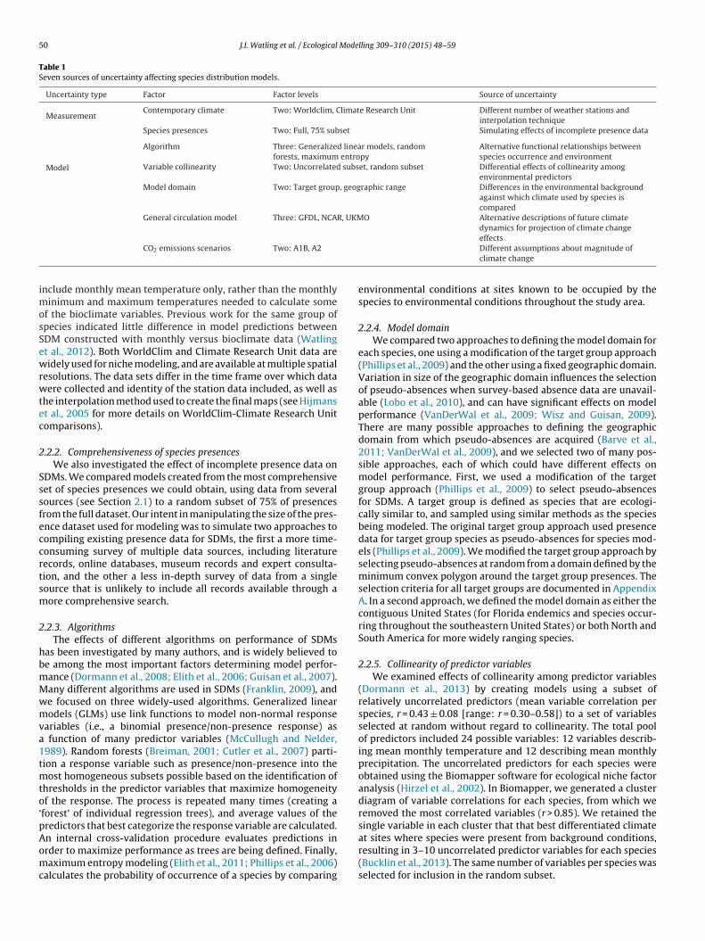

50 J.I. Watling et al. / Ecological Modelling 309–310 (2015) 48–59

Table 1Seven sources of uncertainty affecting species distribution models.

Uncertainty type Factor Factor levels Source of uncertainty

MeasurementContemporary climate Two: Worldclim, Climate Research Unit Different number of weather stations and

interpolation techniqueSpecies presences Two: Full, 75% subset Simulating effects of incomplete presence data

Model

Algorithm Three: Generalized linear models, randomforests, maximum entropy

Alternative functional relationships betweenspecies occurrence and environment

Variable collinearity Two: Uncorrelated subset, random subset Differential effects of collinearity amongenvironmental predictors

Model domain Two: Target group, geographic range Differences in the environmental backgroundagainst which climate used by species iscompared

General circulation model Three: GFDL, NCAR, UKMO Alternative descriptions of future climatedynamics for projection of climate change

imosSewrwtec

2

Sssfeccrtsm

2

hbmMwmva1tmto‘pAomc

CO2 emissions scenarios Two: A1B, A2

nclude monthly mean temperature only, rather than the monthlyinimum and maximum temperatures needed to calculate some

f the bioclimate variables. Previous work for the same group ofpecies indicated little difference in model predictions betweenDM constructed with monthly versus bioclimate data (Watlingt al., 2012). Both WorldClim and Climate Research Unit data areidely used for niche modeling, and are available at multiple spatial

esolutions. The data sets differ in the time frame over which dataere collected and identity of the station data included, as well as

he interpolation method used to create the final maps (see Hijmanst al., 2005 for more details on WorldClim-Climate Research Unitomparisons).

.2.2. Comprehensiveness of species presencesWe also investigated the effect of incomplete presence data on

DMs. We compared models created from the most comprehensiveet of species presences we could obtain, using data from severalources (see Section 2.1) to a random subset of 75% of presencesrom the full dataset. Our intent in manipulating the size of the pres-nce dataset used for modeling was to simulate two approaches toompiling existing presence data for SDMs, the first a more time-onsuming survey of multiple data sources, including literatureecords, online databases, museum records and expert consulta-ion, and the other a less in-depth survey of data from a singleource that is unlikely to include all records available through aore comprehensive search.

.2.3. AlgorithmsThe effects of different algorithms on performance of SDMs

as been investigated by many authors, and is widely believed toe among the most important factors determining model perfor-ance (Dormann et al., 2008; Elith et al., 2006; Guisan et al., 2007).any different algorithms are used in SDMs (Franklin, 2009), ande focused on three widely-used algorithms. Generalized linearodels (GLMs) use link functions to model non-normal response

ariables (i.e., a binomial presence/non-presence response) as function of many predictor variables (McCullugh and Nelder,989). Random forests (Breiman, 2001; Cutler et al., 2007) parti-ion a response variable such as presence/non-presence into the

ost homogeneous subsets possible based on the identification ofhresholds in the predictor variables that maximize homogeneityf the response. The process is repeated many times (creating a

forest’ of individual regression trees), and average values of theredictors that best categorize the response variable are calculated.

n internal cross-validation procedure evaluates predictions inrder to maximize performance as trees are being defined. Finally,aximum entropy modeling (Elith et al., 2011; Phillips et al., 2006)

alculates the probability of occurrence of a species by comparing

effectsDifferent assumptions about magnitude ofclimate change

environmental conditions at sites known to be occupied by thespecies to environmental conditions throughout the study area.

2.2.4. Model domainWe compared two approaches to defining the model domain for

each species, one using a modification of the target group approach(Phillips et al., 2009) and the other using a fixed geographic domain.Variation in size of the geographic domain influences the selectionof pseudo-absences when survey-based absence data are unavail-able (Lobo et al., 2010), and can have significant effects on modelperformance (VanDerWal et al., 2009; Wisz and Guisan, 2009).There are many possible approaches to defining the geographicdomain from which pseudo-absences are acquired (Barve et al.,2011; VanDerWal et al., 2009), and we selected two of many pos-sible approaches, each of which could have different effects onmodel performance. First, we used a modification of the targetgroup approach (Phillips et al., 2009) to select pseudo-absencesfor SDMs. A target group is defined as species that are ecologi-cally similar to, and sampled using similar methods as the speciesbeing modeled. The original target group approach used presencedata for target group species as pseudo-absences for species mod-els (Phillips et al., 2009). We modified the target group approach byselecting pseudo-absences at random from a domain defined by theminimum convex polygon around the target group presences. Theselection criteria for all target groups are documented in AppendixA. In a second approach, we defined the model domain as either thecontiguous United States (for Florida endemics and species occur-ring throughout the southeastern United States) or both North andSouth America for more widely ranging species.

2.2.5. Collinearity of predictor variablesWe examined effects of collinearity among predictor variables

(Dormann et al., 2013) by creating models using a subset ofrelatively uncorrelated predictors (mean variable correlation perspecies, r = 0.43 ± 0.08 [range: r = 0.30–0.58]) to a set of variablesselected at random without regard to collinearity. The total poolof predictors included 24 possible variables: 12 variables describ-ing mean monthly temperature and 12 describing mean monthlyprecipitation. The uncorrelated predictors for each species wereobtained using the Biomapper software for ecological niche factoranalysis (Hirzel et al., 2002). In Biomapper, we generated a clusterdiagram of variable correlations for each species, from which weremoved the most correlated variables (r > 0.85). We retained thesingle variable in each cluster that that best differentiated climate

at sites where species were present from background conditions,resulting in 3–10 uncorrelated predictor variables for each species(Bucklin et al., 2013). The same number of variables per species wasselected for inclusion in the random subset.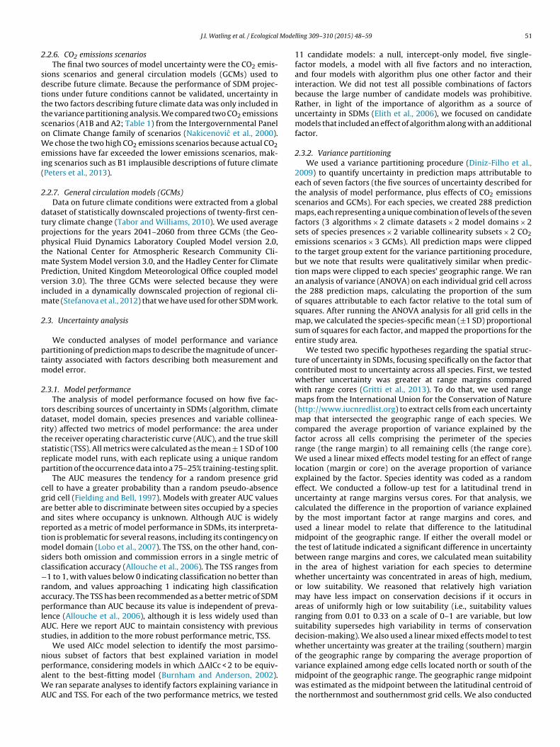

Mode

2

sdtttsoWei(

2

dtpptmPvim

2

ptm

2

tdrtsrp

cgaartmsc−raplAs

npaWA

J.I. Watling et al. / Ecological

.2.6. CO2 emissions scenariosThe final two sources of model uncertainty were the CO2 emis-

ions scenarios and general circulation models (GCMs) used toescribe future climate. Because the performance of SDM projec-ions under future conditions cannot be validated, uncertainty inhe two factors describing future climate data was only included inhe variance partitioning analysis. We compared two CO2 emissionscenarios (A1B and A2; Table 1) from the Intergovernmental Paneln Climate Change family of scenarios (Nakicenovic et al., 2000).e chose the two high CO2 emissions scenarios because actual CO2

missions have far exceeded the lower emissions scenarios, mak-ng scenarios such as B1 implausible descriptions of future climatePeters et al., 2013).

.2.7. General circulation models (GCMs)Data on future climate conditions were extracted from a global

ataset of statistically downscaled projections of twenty-first cen-ury climate change (Tabor and Williams, 2010). We used averagerojections for the years 2041–2060 from three GCMs (the Geo-hysical Fluid Dynamics Laboratory Coupled Model version 2.0,he National Center for Atmospheric Research Community Cli-

ate System Model version 3.0, and the Hadley Center for Climaterediction, United Kingdom Meteorological Office coupled modelersion 3.0). The three GCMs were selected because they werencluded in a dynamically downscaled projection of regional cli-

ate (Stefanova et al., 2012) that we have used for other SDM work.

.3. Uncertainty analysis

We conducted analyses of model performance and varianceartitioning of prediction maps to describe the magnitude of uncer-ainty associated with factors describing both measurement and

odel error.

.3.1. Model performanceThe analysis of model performance focused on how five fac-

ors describing sources of uncertainty in SDMs (algorithm, climateataset, model domain, species presences and variable collinea-ity) affected two metrics of model performance: the area underhe receiver operating characteristic curve (AUC), and the true skilltatistic (TSS). All metrics were calculated as the mean ± 1 SD of 100eplicate model runs, with each replicate using a unique randomartition of the occurrence data into a 75–25% training-testing split.

The AUC measures the tendency for a random presence gridell to have a greater probability than a random pseudo-absencerid cell (Fielding and Bell, 1997). Models with greater AUC valuesre better able to discriminate between sites occupied by a speciesnd sites where occupancy is unknown. Although AUC is widelyeported as a metric of model performance in SDMs, its interpreta-ion is problematic for several reasons, including its contingency on

odel domain (Lobo et al., 2007). The TSS, on the other hand, con-iders both omission and commission errors in a single metric oflassification accuracy (Allouche et al., 2006). The TSS ranges from1 to 1, with values below 0 indicating classification no better than

andom, and values approaching 1 indicating high classificationccuracy. The TSS has been recommended as a better metric of SDMerformance than AUC because its value is independent of preva-

ence (Allouche et al., 2006), although it is less widely used thanUC. Here we report AUC to maintain consistency with previoustudies, in addition to the more robust performance metric, TSS.

We used AICc model selection to identify the most parsimo-ious subset of factors that best explained variation in model

erformance, considering models in which �AICc < 2 to be equiv-lent to the best-fitting model (Burnham and Anderson, 2002).e ran separate analyses to identify factors explaining variance in

UC and TSS. For each of the two performance metrics, we tested

lling 309–310 (2015) 48–59 51

11 candidate models: a null, intercept-only model, five single-factor models, a model with all five factors and no interaction,and four models with algorithm plus one other factor and theirinteraction. We did not test all possible combinations of factorsbecause the large number of candidate models was prohibitive.Rather, in light of the importance of algorithm as a source ofuncertainty in SDMs (Elith et al., 2006), we focused on candidatemodels that included an effect of algorithm along with an additionalfactor.

2.3.2. Variance partitioningWe used a variance partitioning procedure (Diniz-Filho et al.,

2009) to quantify uncertainty in prediction maps attributable toeach of seven factors (the five sources of uncertainty described forthe analysis of model performance, plus effects of CO2 emissionsscenarios and GCMs). For each species, we created 288 predictionmaps, each representing a unique combination of levels of the sevenfactors (3 algorithms × 2 climate datasets × 2 model domains × 2sets of species presences × 2 variable collinearity subsets × 2 CO2emissions scenarios × 3 GCMs). All prediction maps were clippedto the target group extent for the variance partitioning procedure,but we note that results were qualitatively similar when predic-tion maps were clipped to each species’ geographic range. We ranan analysis of variance (ANOVA) on each individual grid cell acrossthe 288 prediction maps, calculating the proportion of the sumof squares attributable to each factor relative to the total sum ofsquares. After running the ANOVA analysis for all grid cells in themap, we calculated the species-specific mean (±1 SD) proportionalsum of squares for each factor, and mapped the proportions for theentire study area.

We tested two specific hypotheses regarding the spatial struc-ture of uncertainty in SDMs, focusing specifically on the factor thatcontributed most to uncertainty across all species. First, we testedwhether uncertainty was greater at range margins comparedwith range cores (Gritti et al., 2013). To do that, we used rangemaps from the International Union for the Conservation of Nature(http://www.iucnredlist.org) to extract cells from each uncertaintymap that intersected the geographic range of each species. Wecompared the average proportion of variance explained by thefactor across all cells comprising the perimeter of the speciesrange (the range margin) to all remaining cells (the range core).We used a linear mixed effects model testing for an effect of rangelocation (margin or core) on the average proportion of varianceexplained by the factor. Species identity was coded as a randomeffect. We conducted a follow-up test for a latitudinal trend inuncertainty at range margins versus cores. For that analysis, wecalculated the difference in the proportion of variance explainedby the most important factor at range margins and cores, andused a linear model to relate that difference to the latitudinalmidpoint of the geographic range. If either the overall model orthe test of latitude indicated a significant difference in uncertaintybetween range margins and cores, we calculated mean suitabilityin the area of highest variation for each species to determinewhether uncertainty was concentrated in areas of high, medium,or low suitability. We reasoned that relatively high variationmay have less impact on conservation decisions if it occurs inareas of uniformly high or low suitability (i.e., suitability valuesranging from 0.01 to 0.33 on a scale of 0–1 are variable, but lowsuitability supersedes high variability in terms of conservationdecision-making). We also used a linear mixed effects model to testwhether uncertainty was greater at the trailing (southern) marginof the geographic range by comparing the average proportion of

variance explained among edge cells located north or south of themidpoint of the geographic range. The geographic range midpointwas estimated as the midpoint between the latitudinal centroid ofthe northernmost and southernmost grid cells. We also conducted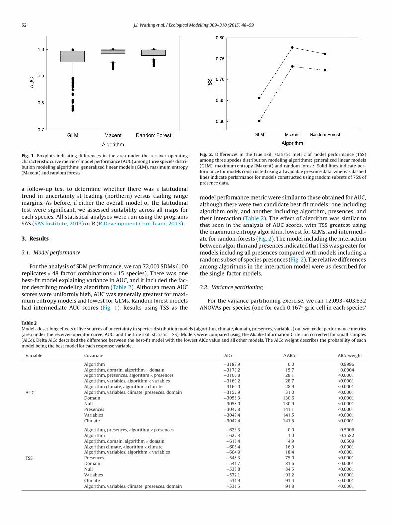

52 J.I. Watling et al. / Ecological Modelling 309–310 (2015) 48–59

Fig. 1. Boxplots indicating differences in the area under the receiver operatingcb(

atmteS

3

3

rbtsmh

Fig. 2. Differences in the true skill statistic metric of model performance (TSS)among three species distribution modeling algorithms: generalized linear models(GLM), maximum entropy (Maxent) and random forests. Solid lines indicate per-

TM((m

haracteristic curve metric of model performance (AUC) among three species distri-ution modeling algorithms: generalized linear models (GLM), maximum entropyMaxent) and random forests.

follow-up test to determine whether there was a latitudinalrend in uncertainty at leading (northern) versus trailing range

argins. As before, if either the overall model or the latitudinalest were significant, we assessed suitability across all maps forach species. All statistical analyses were run using the programsAS (SAS Institute, 2013) or R (R Development Core Team, 2013).

. Results

.1. Model performance

For the analysis of SDM performance, we ran 72,000 SDMs (100eplicates × 48 factor combinations × 15 species). There was oneest-fit model explaining variance in AUC, and it included the fac-

or describing modeling algorithm (Table 2). Although mean AUCcores were uniformly high, AUC was generally greatest for maxi-um entropy models and lowest for GLMs. Random forest models

ad intermediate AUC scores (Fig. 1). Results using TSS as the

able 2odels describing effects of five sources of uncertainty in species distribution models (alg

area under the receiver-operator curve, AUC, and the true skill statistic, TSS). Models wAICc). Delta AICc described the difference between the best-fit model with the lowest A

odel being the best model for each response variable.

Variable Covariate

AUC

Algorithm

Algorithm, domain, algorithm × domain

Algorithm, presences, algorithm × presences

Algorithm, variables, algorithm × variables

Algorithm climate, algorithm × climate

Algorithm, variables, climate, presences, domain

Domain

Null

Presences

Variables

Climate

TSS

Algorithm, presences, algorithm × presences

Algorithm

Algorithm, domain, algorithm × domain

Algorithm climate, algorithm × climate

Algorithm, variables, algorithm × variables

Presences

Domain

Null

Variables

Climate

Algorithm, variables, climate, presences, domain

formance for models constructed using all available presence data, whereas dashedlines indicate performance for models constructed using random subsets of 75% ofpresence data.

model performance metric were similar to those obtained for AUC,although there were two candidate best-fit models: one includingalgorithm only, and another including algorithm, presences, andtheir interaction (Table 2). The effect of algorithm was similar tothat seen in the analysis of AUC scores, with TSS greatest usingthe maximum entropy algorithm, lowest for GLMs, and intermedi-ate for random forests (Fig. 2). The model including the interactionbetween algorithm and presences indicated that TSS was greater formodels including all presences compared with models including arandom subset of species presences (Fig. 2). The relative differencesamong algorithms in the interaction model were as described forthe single-factor models.

3.2. Variance partitioning

For the variance partitioning exercise, we ran 12,093–403,832ANOVAs per species (one for each 0.167◦ grid cell in each species’

orithm, climate, domain, presences, variables) on two model performance metricsere compared using the Akaike Information Criterion corrected for small samplesICc value and all other models. The AICc weight describes the probability of each

AICc �AICc AICc weight

−3188.9 0.0 0.9996−3173.2 15.7 0.0004−3160.8 28.1 <0.0001−3160.2 28.7 <0.0001−3160.0 28.9 <0.0001−3157.9 31.0 <0.0001−3058.3 130.6 <0.0001−3058.0 130.9 <0.0001−3047.8 141.1 <0.0001−3047.4 141.5 <0.0001−3047.4 141.5 <0.0001

−623.3 0.0 0.5906−622.3 1.0 0.3582−618.4 4.9 0.0509−606.4 16.9 0.0001−604.9 18.4 <0.0001−548.3 75.0 <0.0001−541.7 81.6 <0.0001−538.8 84.5 <0.0001−532.1 91.2 <0.0001−531.9 91.4 <0.0001−531.5 91.8 <0.0001

J.I. Watling et al. / Ecological Modelling 309–310 (2015) 48–59 53

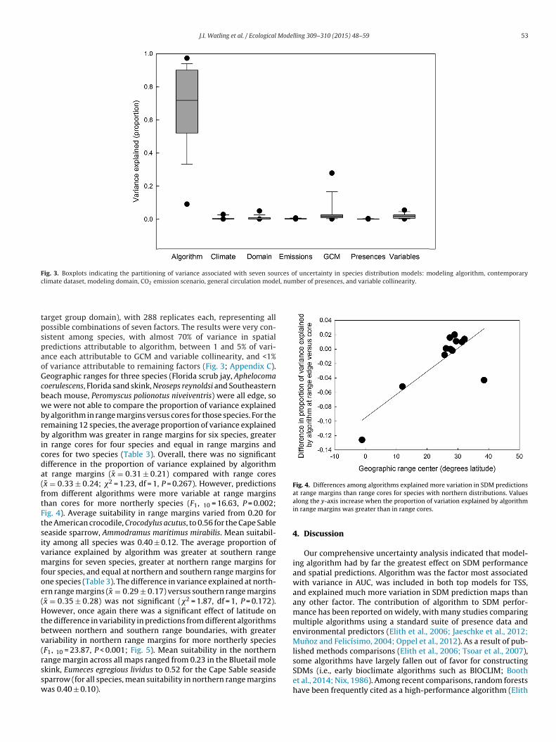
Fig. 3. Boxplots indicating the partitioning of variance associated with seven sources of uncertainty in species distribution models: modeling algorithm, contemporaryc l, number of presences, and variable collinearity.

tpspaoGcbwbrbicda(ftFtsivmfoe(Htbv(rssw

Fig. 4. Differences among algorithms explained more variation in SDM predictions

limate dataset, modeling domain, CO2 emission scenario, general circulation mode

arget group domain), with 288 replicates each, representing allossible combinations of seven factors. The results were very con-istent among species, with almost 70% of variance in spatialredictions attributable to algorithm, between 1 and 5% of vari-nce each attributable to GCM and variable collinearity, and <1%f variance attributable to remaining factors (Fig. 3; Appendix C).eographic ranges for three species (Florida scrub jay, Aphelocomaoerulescens, Florida sand skink, Neoseps reynoldsi and Southeasterneach mouse, Peromyscus polionotus niveiventris) were all edge, soe were not able to compare the proportion of variance explained

y algorithm in range margins versus cores for those species. For theemaining 12 species, the average proportion of variance explainedy algorithm was greater in range margins for six species, greater

n range cores for four species and equal in range margins andores for two species (Table 3). Overall, there was no significantifference in the proportion of variance explained by algorithmt range margins (x = 0.31 ± 0.21) compared with range coresx = 0.33 ± 0.24; �2 = 1.23, df = 1, P = 0.267). However, predictionsrom different algorithms were more variable at range marginshan cores for more northerly species (F1, 10 = 16.63, P = 0.002;ig. 4). Average suitability in range margins varied from 0.20 forhe American crocodile, Crocodylus acutus, to 0.56 for the Cape Sableeaside sparrow, Ammodramus maritimus mirabilis. Mean suitabil-ty among all species was 0.40 ± 0.12. The average proportion ofariance explained by algorithm was greater at southern rangeargins for seven species, greater at northern range margins for

our species, and equal at northern and southern range margins forne species (Table 3). The difference in variance explained at north-rn range margins (x = 0.29 ± 0.17) versus southern range marginsx = 0.35 ± 0.28) was not significant (�2 = 1.87, df = 1, P = 0.172).owever, once again there was a significant effect of latitude on

he difference in variability in predictions from different algorithmsetween northern and southern range boundaries, with greaterariability in northern range margins for more northerly speciesF1, 10 = 23.87, P < 0.001; Fig. 5). Mean suitability in the northern

ange margin across all maps ranged from 0.23 in the Bluetail molekink, Eumeces egregious lividus to 0.52 for the Cape Sable seasideparrow (for all species, mean suitability in northern range marginsas 0.40 ± 0.10).

at range margins than range cores for species with northern distributions. Valuesalong the y-axis increase when the proportion of variation explained by algorithmin range margins was greater than in range cores.

4. Discussion

Our comprehensive uncertainty analysis indicated that model-ing algorithm had by far the greatest effect on SDM performanceand spatial predictions. Algorithm was the factor most associatedwith variance in AUC, was included in both top models for TSS,and explained much more variation in SDM prediction maps thanany other factor. The contribution of algorithm to SDM perfor-mance has been reported on widely, with many studies comparingmultiple algorithms using a standard suite of presence data andenvironmental predictors (Elith et al., 2006; Jaeschke et al., 2012;Munoz and Felicísimo, 2004; Oppel et al., 2012). As a result of pub-lished methods comparisons (Elith et al., 2006; Tsoar et al., 2007),

some algorithms have largely fallen out of favor for constructingSDMs (i.e., early bioclimate algorithms such as BIOCLIM; Boothet al., 2014; Nix, 1986). Among recent comparisons, random forestshave been frequently cited as a high-performance algorithm (Elith

54 J.I. Watling et al. / Ecological Modelling 309–310 (2015) 48–59Ta

ble

3Su

mm

ary

of

vari

ance

par

titi

onin

g

for

15

spec

ies

of

thre

aten

ed

and

end

ange

red

vert

ebra

te

spec

ies

in

the

sou

thea

ster

n

USA

. Th

e

pro

por

tion

of

vari

ance

asso

ciat

ed

wit

h

each

of

seve

n

fact

ors

(col

um

ns

3–9)

acro

ss

288

pre

dic

tion

map

s

in

each

spec

ies’

targ

et

grou

p

dom

ain

(det

erm

ined

ind

ivid

ual

ly

for

each

spec

ies

as

the

leas

t

con

vex

pol

ygon

enco

mp

assi

ng

occu

rren

ces

of

ecol

ogic

ally

sim

ilar

spec

ies)

. Col

um

ns

10–1

1

com

par

e

vari

ance

asso

ciat

ed

wit

hd

iffe

ren

ces

amon

g

thre

e

algo

rith

ms

(gen

eral

ized

lin

ear

mod

els,

max

imu

m

entr

opy,

and

ran

dom

fore

sts)

in

geog

rap

hic

ran

ge

mar

gin

s

and

core

s,

and

colu

mn

s

12–1

3

com

par

e

vari

ance

amon

g

algo

rith

ms

at

nor

ther

n

and

sou

ther

nra

nge

mar

gin

s.

Ran

ges

for

thre

e

spec

ies

wer

e

all e

dge

, so

geog

rap

hic

ran

ge

anal

yses

wer

e

not

per

form

ed.

Spec

ies

Targ

et

grou

p

anal

yses

Geo

grap

hic

ran

ge

anal

yses

Scie

nti

fic

nam

eC

omm

on

nam

eA

lgor

ith

m

Cli

mat

e

Dom

ain

CO

2em

issi

ons

scen

ario

GC

M

Pres

ence

s

Var

iabl

es

Mar

gin

Cor

e

Nor

ther

nm

argi

nSo

uth

ern

mar

gin

Am

byst

oma

cing

ulat

umFl

atw

ood

s

sala

man

der

0.09

0.03

<0.0

1<0

.01

0.28

<0.0

1<0

.01

0.02

0.01

<0.0

1 0.

04A

mm

odra

mus

mar

itim

us

mir

abili

s

Cap

e

Sabl

e

seas

ide

spar

row

0.97

<0.0

1

<0.0

1

<0.0

1

<0.0

1

<0.0

1

<0.0

1

0.39

0.40

0.37

0.42

Am

mod

ram

us

sava

nnar

um

flori

danu

s

Flor

ida

gras

shop

per

spar

row

0.52

<0.0

1

<0.0

1

<0.0

1

0.09

<0.0

1

0.02

0.21

0.21

0.22

0.19

Aph

eloc

oma

coer

ules

cens

Flor

ida

scru

b

jay

0.70

<0.0

10.

01<0

.01

0.02

<0.0

1<0

.01

NA

NA

NA

NA

Char

adri

us

mel

odus

Pip

ing

plo

ver

0.72

<0.0

1

<0.0

1

<0.0

1

0.03

<0.0

1

0.05

0.28

0.32

0.29

0.26

Croc

odyl

us

acut

usA

mer

ican

croc

odil

e0.

86<0

.01

<0.0

1<0

.01

0.01

<0.0

1

0.02

0.71

0.77

0.64

0.85

Dry

mar

chon

cora

is

coup

eri

East

ern

ind

igo

snak

e

0.72

<0.0

1

<0.0

1

<0.0

1

0.02

<0.0

1

<0.0

1

0.28

0.26

0.31

0.23

Eum

eces

egre

gius

livid

usB

luet

ail m

ole

skin

k0.

50<0

.01

<0.0

1

<0.0

1

0.02

<0.0

1

0.02

0.41

0.40

0.39

0.44

Myc

teri

a

amer

ican

aW

ood

stor

k0.

76<0

.01

<0.0

1<0

.01

0.04

<0.0

10.

020.

63

0.75

0.51

0.92

Neo

seps

reyn

olds

i

Flor

ida

san

d

skin

k

0.92

<0.0

1

<0.0

1

<0.0

1

<0.0

1

<0.0

1

<0.0

1

NA

NA

NA

NA

Pero

mys

cus

polio

notu

s

niev

even

tris

Sou

thea

ster

n

beac

h

mou

se0.

71<0

.01

<0.0

1<0

.01

0.02

<0.0

10.

03

NA

NA

NA

NA

Pico

ides

bore

alis

Red

-coc

kad

ed

woo

dp

ecke

r

0.50

0.02

0.04

9

<0.0

1

<0.0

1

<0.0

1

0.04

0.24

0.23

0.19

0.33

Poly

boru

s

plan

cus

audu

boni

iA

ud

ubo

n’s

cres

ted

cara

cara

0.69

<0.0

1<0

.01

<0.0

1

0.03

<0.0

1

0.03

0.17

0.15

0.16

0.17

Pum

a

cono

colo

r

cory

iFl

orid

a

pan

ther

0.91

<0.0

1

<0.0

1

<0.0

1

<0.0

1

<0.0

1

<0.0

1

0.32

0.31

0.32

0.32

Ros

trha

mus

soci

abili

s

plum

beus

Ever

glad

es

snai

l kit

e

0.9

<0.0

1

<0.0

1

<0.0

1

<0.0

1

<0.0

1 <0

.01

0.06

0.06

0.11

0.02

Fig. 5. Differences among algorithms explained more variation in SDM predictionsat northern (leading) range margins compared with southern (trailing) range mar-gins for species with northern distributions. Values along the y-axis increase when

the proportion of variation explained by algorithm in northern range margins wasgreater than in southern range margins.

et al., 2008; Kampichler et al., 2010; Valle et al., 2013). Althoughstill evolving, niche models constructed using Bayesian and otherapproaches (Royle et al., 2012) may one day outperform machinelearning algorithms such as maximum entropy and random forests(Fitzpatrick et al., 2013).

The clear implication of the factorial experiment we conductedis that users should compare results from multiple algorithms whenconstructing SDMs, and use a subset of the highest-performingalgorithms for extrapolation. Advances in the software used formodeling make it possible to run models for many algorithmsin a single package (e.g., the BIOMOD package for R statisticalsoftware, which can create prediction using 10 different algo-rithms, Thuiller et al., 2014). Given the overwhelming importanceof algorithm demonstrated in this and other studies, use of asingle algorithm without explicitly comparing its performance toothers may easily lead to spurious predictions. Ensembles of high-performing algorithms often have higher performance than any onecomponent algorithm (Marmion et al., 2009). However, even high-performing algorithms may have different characteristic behaviorswhen extrapolated in space and time. For example, maximumentropy can be prone to overprediction (Fitzpatrick et al., 2013),whereas random forest models often have high specificity (Bucklinet al., 2015). It is probably best to use a subset of multiple algo-rithms for which preliminary model performance metrics indicatehigh performance for the species being modeled (Marmion et al.,2009).

A previous study compared uncertainty associated with fourfactors: the reliability of the occurrence data, collinearity amongenvironmental predictors, algorithm, and variable selection tech-niques on SDM predictions for the Great Grey Shrike (Laniusexcubitor) in east-central Germany (Dormann et al., 2008). Forthat one species in a relatively small region (∼17,000 km2), differ-ences among algorithms contributed to approximately 50% of thevariation in model performance (AUC), with differences in the reli-ability of occurrence data and variable collinearity explaining mostof the rest of the variation in AUC in roughly equal proportions.Alternative variable selection approaches contributed negligibly todifferences in AUC in that study. Our results are consistent with

those of the previous study (Dormann et al., 2008) insofar as wealso found that algorithm explained most of the variance in SDMperformance. However, our study of 15 species and seven sources

Mode

ordrwt

pcFl2ecsdlct2dvenidn

mbch(pd5wsdSsi1paeiucipisd

gniaiausamo

J.I. Watling et al. / Ecological

f uncertainty revealed that factors other than algorithm explainedelatively little variation in SDMs, especially in the analysis of pre-iction maps. Although the species pool used for our analyses iselevant from the perspective of applied conservation, more workith different species in varying geographical contexts is needed

o generalize the results of the current study.In contrast with the overwhelming effect of algorithm on SDM

erformance and predictions, many putative sources of uncertaintyontributed little to variation among model runs in the experiment.or example, several recent studies have focused on variable col-inearity as a major source of uncertainty in SDMs (Braunisch et al.,013; Cruz-Cárdenas et al., 2014; Dormann et al., 2013; Heikkinent al., 2006). Machine learning algorithms may be more tolerant ofollinearity than other modeling methods (Dormann et al., 2013),o we may have seen greater effects of collinearity if we had used aifferent group of algorithms for comparison. Nonetheless, regard-

ess of the algorithm used, it is best to take precautions againstollinearity, and simply using a single variable to represent mul-iple correlated variables can be a good approach (Dormann et al.,013). Another well-known source of variation in SDMs is differentescriptions of future climate. A previous study suggested that highariation in SDM predictions among GCMs precluded the ability tovaluate alternatives associated with different CO2 emissions sce-arios (Real et al., 2010). Our study suggests that even more caution

s necessary when evaluating alternative future conditions, becauseifferences in spatial predictions among GCMs and emissions sce-arios are swamped by differences among algorithms.

We found that the number of presence observations included inodels was a factor, along with algorithm, in one of two candidate

est-fit models explaining variance in TSS. We found that modelsonstructed from a random subset of 75% of all species presencesad lower performance than models using the full presence datasetFig. 2). The decrease in TSS was consistent among algorithms. Arevious study investigating variously sized subsets of presenceata for rare species in California found that even models using0% of presences performed comparably to models constructedith the complete training dataset (Hernandez et al., 2006). The

ame study found that different algorithms responded somewhatifferently to variation in the size of the presence dataset used forDM training. It is possible that the more dramatic decline in TSSeen in the reduced models we created may be a result of smallernitial sample sizes for some of the species we tested (nine out of5 species in the current study had fewer than the minimum 150resences used in the California study; Hernandez et al., 2006). It islso possible that the effects of presence subsets are more appar-nt using the TSS performance metric. Presences were not a factorn best-fit models for AUC in our study. Few studies report resultssing TSS, however, so it is difficult to know how our observationsompare with other comprehensive studies. Given the potentialmportance of species presences observed in this study, and theossibility of erroneous predictions resulting from sampling bias

n the presence data (Fourcade et al., 2014; Phillips et al., 2009), weuggest that care be invested in compiling the most robust presenceatasets possible.

We found that variation in SDM predictions at range mar-ins, particularly leading (northern) range margins, was greater fororthern species compared with southern species. Climate suitabil-

ty in northern range margins was moderate, averaging 0.42 ± 0.09mong all species. The observation that different algorithms varyn their predictions at the leading end of the geographic ranges inreas of moderate suitability suggests potential ambiguity whensing SDMs to forecast climate-induced range shifts for northern

pecies. High variability around a value (0.42) near the middle of

distribution (suitability ranges from 0 to 1) suggests that someaps will predict high suitability in the northern range margin, and

thers will predict low suitability, resulting in a moderate estimate

lling 309–310 (2015) 48–59 55

of suitability, on average. If we consider the scenario just describedwhen using SDM prediction maps to locate new protected areasin areas of high future suitability for species at risk for negativeeffects of climate change (Carroll et al., 2010), we can see that theoptimal reserve design may be highly contingent on the algorithmused to estimate suitability. It is important to select a subset ofhigh-performing algorithms when using SDMs for conservationdecision-making, and consider average predictions across anensemble of models to reduce uncertainty (Marmion et al., 2009).However, this study suggests that even high-performing algo-rithms can vary in their spatial predictions, with high uncertaintyconcentrated in leading range margins for species with morenorthern distributions. We note that although we documentedgreater uncertainty in prediction maps at leading range margins forspecies with more northern distributions, the species we modeledare concentrated in the southern USA, and we do not know if thelatitudinal trends we describe here apply to species in the rest of thecountry.

4.1. Conclusions

In summary, our comprehensive factorial experiment identifiedmodeling algorithm as the most importance source of uncertaintyin performance and predictions from SDMs, outstripping impor-tance of other factors such as the choice of GCM or CO2 emissionsscenario. There was also an indication that the comprehensive-ness of the presence dataset used for modeling can consistentlyinfluence performance of SDMs. The results of this study suggestthat SDM users will be well-served by (1) use multiple algo-rithms for modeling rather than relying on predictions from asingle algorithm, (2) compiling the most comprehensive dataset ofspecies presences possible, acquiring records from multiple sourcesincluding the primary literature, expert consultation, and multi-ple museum databases, and (3) explicitly evaluating uncertainty inSDM predictions at leading range margins. When using SDMs forspatial prioritization of conservation actions, it is best to describeenvironmental suitability based on areas where predictions frommultiple algorithms intersect, given the wide variation in spatialpredictions from different algorithms.

Acknowledgments

Funding for this work was provided by the U.S. Fish and WildlifeService, Everglades and Dry Tortugas National Park through theSouth Florida and Caribbean Cooperative Ecosystem Studies Unit,and USGS Greater Everglades Priority Ecosystem Science. The viewsin this paper do not necessarily represent the views of the U.S. Fishand Wildlife Service. Use of trade, product, or firm names does notimply endorsement by the US Government.

Appendix A.

Target group definition of the modeling domain for 15 speciesof threatened or endangered terrestrial vertebrate species in thesoutheastern USA. Shapefiles of target group masks are availableupon request from the first author.

We used a modification of the target group approach (Phillipset al., 2009) to define an ecologically relevant domain for modeldevelopment because recent work has shown that predictions fromclimate envelope models may be affected by the arbitrary selectionof modeling domain (VanDerWal et al., 2009). Briefly, the target

group approach specifies that the ‘absence’ data used to definespecies-environment relationships be obtained using presencesof ecologically similar species sampled using similar methods asthe focal species being modeled (Phillips et al., 2009). In order to

5 Mode

ksauem1p

ttAftaCsccaisporgiactstf2

6 J.I. Watling et al. / Ecological

eep the number of ‘absences’ used for modeling constant acrosspecies (using the commonly-invoked number of 10,000 pseudo-bsences), we modified the target group approach. Rather thansing target group occurrences as ‘absences’ in our species mod-ls, we compiled the occurrences of target group species, drew ainimum convex polygon around those absences, and sampled

0,000 pseudo-absences at random within the minimum convexolygon.

We defined the target group area for the Florida panther ashe composite range of all New World felids. The target group forhe Cape Sable seaside sparrow was defined as the full range of. maritimus, for the Florida grasshopper sparrow as the range of

ull species Ammodramus savannarum, for the Florida scrub jay ashe composite range of all Aphelocoma spp, for the piping plovers the composite range of all New World species of the genusharadrius, for the wood stork as the composite range of New Worldtorks (family Ciconiidae), for the Audubon crested caracara as theombined range of the northern and southern caracara (Caracaraheriway and Caracara plancus), for the Everglades snail kite asll New World species of the subfamily Milvinae, for the whoop-ng crane as the composite range on New World species of theuborder Grui (e.g., the New World cranes, limpkins and trum-eters), and the red-cockaded woodpecker as the composite rangef closely-related Picoides villosus and P. albolarvatus based on aecent Picoides phylogeny (Weibel and Moore, 2002). The targetroup range for the American crocodile was defined as the compos-te range of all New World crocodilians, for the bluetail mole skinknd sand skink as North American species of the Eumeces + Neosepslade from a recent skink phylogeny (Brandley et al., 2005), and forhe eastern indigo snake as the composite range of closely relatedpecies (Coluber constrictor, Spilotes pullatus, Phyllorynchus decur-

atus, Masticophis flagellum and Drymarchon corais) as determinedrom two recent phylogenies (Lawson et al., 2005; Alfaro et al.,008).

Species N Source

GBIF BERDS ORNIS Herp

MammalsFlorida panther 109 4

Southeastern beach mouse 14 2

BirdsCape Sable seaside sparrow 17 2

Florida grasshopper sparrow 26 4

Florida scrub jay 209 122 3

Piping plover 867 749

Wood stork 1601 1464 125

Audubon crested caracara 162 149

Everglades snail kite 106 106Red-cockaded woodpecker 531 531

Amphibians and reptilesFlatwoods salamander 9 4

American crocodile 124 37 2 1

Bluetail mole skink 20

Sand skink 21 10

Eastern indigo snake 278 3

GBIF: Global Biodiversity Information Fund: www.gbif.org.Zip Code Zoo: www.zipcodezoo.com.FWRI: Fish and Wildlife Research Institute: research.myfwc.com.MANIS: Mammal Networked Information Service: www.manisnet.org.BERDS: Biodiversity and Environmental Resource Data System of Belize: www.biodiverHerpNet: www.herpnet.org.ORNIS: Ornithology Networked Information Service: www.ornisnet.org.FLMNH: Florida Museum of Natural History: www.flmnh.ufl.edu.

lling 309–310 (2015) 48–59

We chose more exclusive taxonomic groupings for the defini-tion for some species because the family-level range would resultin a domain covering most of the Western Hemisphere, an areamuch larger than the observed range of the species. Georeferencedobservations of all target group species were obtained from a sin-gle online database (the Global Biodiversity Information Facility,www.gbif.org), data were preprocessed as described above, andthe 100% minimum convex polygon defining each target group wascalculated.

ReferencesAlfaro, M.E., Karns, D.R., Voris, H.K., Brock, C.D., Stuart, B.L., 2008.

Phylogeny, evolutionary history, and biogeography of Oriental-Australian rear-fanged water snakes (Colubroidea: Homalopsidae)inferred from mitochondrial and nuclear DNA sequences. Molecu-lar Phylogenetics and Evolution 46, 576–593.

Brandley, M.C., Schmitz, A., Reeder, T.W., 2005. PartitionedBayesian analyses, partition choice, and the phylogenetic relation-ships of scincid lizards. Systematic Biology 54, 373–390.

Lawson, R., Slowinski, J.B., Crother, B.I., Burbrink, F.T., 2005.Phylogeny of the Colubroidea (Serpentes): new evidence frommitochondrial and nuclear genes. Molecular Phylogenetics andEvolution 37, 581–601.

VanDerWal, J., Shoo, L.P., Graham, C., Williams, S.E., 2009. Select-ing pseudo-absence data for presence-only distribution modeling:how far should you stray from what you know? Ecological Mod-elling 220, 589–594.

Weibel, A.C., Moore, W.S., 2002. Molecular phylogeny of a cos-mopolitan group of woodpeckers (Genus Picoides) based on COI andcyt b mitochondrial gene sequences. Molecular Phylogenetics andEvolution 22, 65–75.

Appendix B.

The number and source of species observations used for modelconstruction is included in the following table:

Net Zip Code Zoo FLMNH Literature Field observations FWRI

3 14 886 6

2 1322

1 8395 23

1213

572 12

202 9

275

sity.bz.

Mode

A

to

J.I. Watling et al. / Ecological

ppendix C.

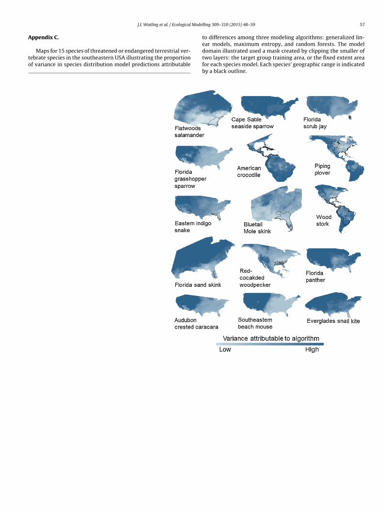
Maps for 15 species of threatened or endangered terrestrial ver-ebrate species in the southeastern USA illustrating the proportionf variance in species distribution model predictions attributable

lling 309–310 (2015) 48–59 57

to differences among three modeling algorithms: generalized lin-ear models, maximum entropy, and random forests. The modeldomain illustrated used a mask created by clipping the smaller oftwo layers: the target group training area, or the fixed extent areafor each species model. Each species’ geographic range is indicatedby a black outline.

5 Mode

R

A

A

A

B

B

B

B

B

BB

B

B

B

C

C

C

C

D

D

D

E

E

E

E

F

F

F

F

G

G

H

8 J.I. Watling et al. / Ecological

eferences

llouche, O., Tsoar, A., Kadmon, R., 2006. Assessing the accuracy of species distribu-tion models: prevalence, kappa and the true skill statistic (TSS). J. Appl. Ecol. 43,1223–1232.

lvarado-Serrano, D.F., Knowles, L.L., 2014. Ecological niche models in phylogeo-graphic studies: applications, advances and precautions. Mol. Ecol. Resour. 14,233–248.

raújo, M.B., Peterson, A.T., 2012. Uses and misuses of bioclimatic envelope model-ing. Ecology 93, 1527–1539.

arve, N., Barve, V., Jiménez-Valverde, A., Lira-Noriega, A., Maher, S.P., Peterson,A.T., Soberón, J., Villalobos, S., 2011. The crucial role of the accessible area inecological niche modeling and species distribution modeling. Ecol. Model. 222,1810–1819.

enscoter, A.M., Reece, J.S., Noss, R.F., Brandt, L.A., Mazzotti, F.J., Romanach, S.S.,Watling, J.I., 2013. Threatened and endangered subspecies with vulnerableecological traits also have high susceptibility to sea level rise and habitat frag-mentation. PLoS ONE 8, e70647.

laustein, R.J., 2008. Biodiversity hotspot: the Florida panhandle. Bioscience 58,784–790.

ooth, T.H., Nix, H.A., Busby, J.R., Hutchinson, M.F., 2014. BIOCLIM: the first speciesdistribution modelling package, its early applications and relevance to mostcurrent MaxEnt studies. Divers. Distrib. 20, 1–9.

raunisch, V., Coppes, J., Arlettaz, R., Suchant, R., Schmid, H., Bollman, K., 2013.Selecting from correlated climate variables: a major source of uncertainty forpredicting species distributions under climate change. Ecography 36, 971–983.

reiman, L., 2001. Random forests. Mach. Learn. 45, 15–32.ucklin, D.B., Basille, M., Benscoter, A.M., Brandt, L.A., Mazzotti, F.J., Romanach, S.S.,

Speroterra, C., Watling, J.I., 2015. Comparing species distribution models con-structed with different subsets of environmental predictors. Divers. Distrib. 21,23–35.

ucklin, D.B., Watling, J.I., Speroterra, C., Brandt, L.A., Mazzotti, F.J., Romanach, S.S.,2013. Climate downscaling effects on predictive ecological models: a case studyfor threatened and endangered vertebrates in the southeastern United States.Reg. Environ. Change 13, 57–68.

uisson, L., Thuiller, W., Casajus, N., Lek, S., Grenouillet, G., 2010. Uncertainty inensemble forecasting of species distribution. Glob. Change Biol. 16, 1145–1157.

urnham, K.P., Anderson, D.R., 2002. Model Selection and Multimodel Inference: APractical Information–Theoretic Approach. Springer, New York, USA.

arroll, C., Dunk, J.R., Moilanen, A., 2010. Optimizing resiliency of reserve networksto climate change: multispecies conservation planning in the Pacific Northwest,USA. Glob. Change Biol. 16, 891–904.

atano, C.P., Romanach, S.S., Beerens, J.M., Pearlstine, L.G., Brandt, L.A., Hart, K.M.,Mazzotti, F.J., Trexler, J.C., 2014. Using scenario planning to evaluate the impactsof climate change on wildlife populations and communities in the Florida Ever-glades. Environ. Manage., http://dx.doi.org/10.1007/s00267-014-0397-5

ruz-Cárdenas, G., López-Mata, L., Villasenor, J.L., Ortiz, E., 2014. Potential speciesdistribution modeling and the use of principal component analysis as predictorvariables. Rev. Mexicana Biodiver. 85, 189–199.

utler, D.R., Edwards Jr., T.C., Beard, K.H., Cutler, A., Hess, K.T., Gibson, J., Lawler, J.J.,2007. Random forests for classification in ecology. Ecology 88, 2783–2792.

iniz-Filho, J.A.F., Bini, L.M., Rangel, T.R., Loyola, R.D., Hof, C., Nogués-Bravo, D.,Araújo, M.B., 2009. Partitioning and mapping uncertainties in ensembles offorecasts of species turnover under climate change. Ecography 32, 897–906.

ormann, C.F., et al., 2013. Collinearity: a review of methods to deal with it and asimulation study evaluating their performance. Ecography 36, 27–46.

ormann, C.F., Purschke, O., García Márquez, J.R., Lautenbach, S., Schröder, S., 2008.Components of uncertainty in species distribution analysis: a case study of theGreat Grey Shrike. Ecology 89, 3371–3386.

lith, J., Burgman, M.A., Regan, H.M., 2002. Mapping epistemic uncertainties andvague concepts in predictions of species distribution. Ecol. Model. 157, 313–329.

lith, J., et al., 2006. Novel methods improve prediction of species’ distributions fromoccurrence data. Ecography 29, 129–151.

lith, J., Leathwick, J.R., Hastie, T., 2008. A working guide to boosted regression trees.J. Anim. Ecol. 77, 802–813.

lith, J., Phillips, S.J., Hastie, T., Dudík, M., Chee, Y.E., Yates, C.J., 2011. A statisticalexplanation of MaxEnt for ecologists. Divers. Distrib. 17, 43–57.

ielding, A.H., Bell, J.F., 1997. A review of methods for the assessment of predictionerrors in conservation presence/absence models. Environ. Conserv. 24, 38–49.

itzpatrick, M.C., Gotelli, N.J., Ellison, A.M., 2013. MaxEnt versus MaxLike: empiricalcomparisons with ant species distributions. Ecosphere 4, 55.

ourcade, Y., Engler, J.O., Rodder, D., Secondi, J., 2014. Mapping species distribu-tions with MAXENT using a geographically biased sample of presence data: aperformance assessment of methods for correcting sampling bias. PLoS ONE 9,e97122.

ranklin, J., 2009. Mapping Species Distributions. Cambridge University Press,Cambridge.

ritti, E.S., Duputié, A., Massol, F., Chuine, I., 2013. Estimating consensus and asso-ciated uncertainty between inherently different species distribution models.Meth. Ecol. Evol. 4, 442–452.

uisan, A., Zimmerman, N.E., Elith, J., Graham, C.H., Phillips, S., Peterson, A.T., 2007.

What matters most for predicting the occurrences of trees: techniques, data, orspecies characteristics? Ecol. Monogr. 77, 615–630.

anspach, J., Kühn, I., Schweiger, O., Pompe, S., Klotz, S., 2011. Geographical pat-terns in prediction errors of species distribution models. Glob. Ecol. Biogeogr.20, 779–788.

lling 309–310 (2015) 48–59

Heikkinen, R.K., Luoto, M., Araújo, M.B., Virkkala, R., Thuiller, W., Sykes, M.T., 2006.Methods and uncertainties in bioclimate envelope modeling under climatechange. Prog. Phys. Geogr. 30, 751–777.

Hernandez, P.A., Graham, C.H., Master, L.L., Albert, D.L., 2006. The effect of samplesize and species characteristics on performance of different species distributionmodeling methods. Ecography 29, 773–785.

Hijmans, R.J., Cameron, S.E., Parra, J.L., Jones, P.G., Jarvis, A., 2005. Very high resolutioninterpolated climate surfaces for global land areas. Int. J. Clim. 25, 1965–1978.

Hirzel, A.H., Hausser, J., Chessel, D., Perrin, N., 2002. Ecological-niche factor analysis:how to compute habitat-suitability maps without absence data? Ecology 83,2027–2036.

Jaeschke, A., Bittner, T., Jentsch, A., Reineking, B., Schlumprecht, H., Beierkuhnlein,C., 2012. Biotic interactions in the face of climate change: a comparison of threemodelling approaches. PLoS ONE, e51472.

Kampichler, C., Wieland, R., Calmé, S., Weissenberger, H., Arriaga-Weiss, S., 2010.Classification in conservation biology: a comparison of five machine-learningmethods. Ecol. Inform. 5, 441–450.

Knight, G.R., Oetting, J.B., Cross, L., 2011. Atlas of Florida’s Natural Heritage – Bio-diversity, Landscapes, Stewardship, and Opportunities. Florida State University,Tallahassee.

Lobo, J.M., Jiménez-Valverde, A., Real, R., 2007. AUC: a misleading measure of the per-formance of predictive distribution models. Glob. Ecol. Biogeogr. 17, 145–151.

Lobo, J.M., Jiménez-Valverde, A., Hortal, J., 2010. The uncertain nature of absencesand their importance in species distribution modelling. Ecography 33, 103–114.

Luoto, M., Virkkala, R., Heikkinen, R.K., 2007. The role of land cover in bioclimaticmodels depends on spatial resolution. Glob. Ecol. Biogeogr. 16, 34–42.

Marmion, M., Parviainen, M., Luoto, M., Heikkinen, R.K., Thuiller, W., 2009. Evalua-tion of consensus methods in predictive species distribution modelling. Divers.Distrib. 15, 59–69.

McCullugh, P., Nelder, J.A., 1989. Generalized Linear Models, second edition.Chapman and Hall, New York, New York, USA.

Munoz, J., Felicísimo, A.M., 2004. Comparison of statistical methods commonly usedin predictive modelling. J. Veg. Sci. 15, 285–292.

Nakicenovic, N., et al., 2000. Intergovernmental Panel on Climate Change SpecialReport on Emissions Scenarios. Cambridge University Press, United Kingdom,Cambridge.

New, M., Lister, D., Hulme, M., Makin, I., 2002. A high-resolution data set of surfaceclimate over global land areas. Clim. Res. 21, 1–25.

Nicholls, R.J., Hanson, S., Herweijer, C., Patmore, N., Hallegatte, S., Corfee-Morlot, J.,Chateau, J., Muir-Wood, R., 2008. Ranking port cities with high exposure andvulnerability to climate extremes: exposure estimates. Environment workingpaper no. 1. Organization for Economic Co-operation and Development, Paris.

Nix, H.A., 1986. A biogeographic analysis of Australian elapid snakes. In: Longmore,R. (Ed.), Atlas of elapid snakes if Australia: Australian flora and fauna series 7.Bureau of Flora and Fauna, Canberra, pp. 4–15.

Oliver, T.H., Gillings, S., Giardello, M., Rapacciuolo, G., Brereton, T.M., Siriwardena,G.M., Roy, D.B., Pywell, R., Fuller, R.J., 2012. Population density but not stabilitycan be predicted from species distribution models. J. Appl. Ecol. 49, 581–590.

Oppel, S., Meirinho, A., Ramírez, I., Gardner, B., O’Connell, A.F., Miller, P.I., Louzao,M., 2012. Comparison of five modelling techniques to predict spatial distributionand abundance of seabirds. Biol. Conserv. 156, 94–104.

Pagel, J., Schurr, F.M., 2012. Forecasting species ranges by statistical estimation ofecological niches and spatial population dynamics. Glob. Ecol. Biogeogr. 21,293–304.

Peters, G.P., Andrew, R.M., Boden, T., Canadell, J.G., Ciais, P., La Quéré, C., Marland,G., Raupach, M.R., Wilson, C., 2013. The challenge to keep global warming below2 ◦C. Nat. Clim. Change 3, 4–6.

Phillips, S.J., Anderson, R.P., Schapire, R.E., 2006. Maximum entropy modeling ofspecies geographic distributions. Ecol. Model. 190, 231–259.

Phillips, S.J., Dudík, M., Elith, J., Graham, C.H., Lehmann, A., Leathwick, J.,Ferrier, S., 2009. Sample selection bias and presence-only distribution mod-els: implications for background and pseudo-absence data. Ecol. Appl. 19,181–197.

R Development Core Team, 2013. R: A Language and Environment for Statisti-cal Computing. R Foundation for Statistical Computing, Austria, Vienna, http://www.r-project.org (accessed 20.05.13).

Real, R., Márquez, A.L., Olivero, J., Estrada, A., 2010. Species distribution modelsin climate change scenarios are still not useful for informing public policy: anuncertainty assessment using fuzzy logic. Ecography 33, 304–314.

Reece, J.S., Noss, R.F., Oetting, J., Hoctor, T., Volk, M., 2013. A vulnerability assessmentof 300 species in Florida: threats from sea level rise, land use and climate change.PLoS ONE 8, e80658.

Royle, J.A., Chandler, R.B., Yackulic, C., Nichols, J.D., 2012. Likelihood analysis ofspecies occurrence probability from presence-only data for modelling speciesdistributions. Methods Ecol. Evol. 3, 545–554.

SAS Institute, 2013. SAS 9.4 User’s Guide. Cary, NC.Shirley, S.M., Yang, Z., Hutchinson, R.A., Alexander, J.D., McGarigal, K., Betts, M.G.,

2013. Species distribution modeling for the people: unclassified landsat TMimagery predicts bird occurrence at fine resolutions. Divers. Distrib. 2013,1–12.

Stefanova, L., Misra, V., Chan, S., Griffin, M., O’Brien, J.J., Smith III, T.J., 2012. A proxy forhigh-resolution regional reanalysis for the southeast United States: assessment

of precipitation variability in dynamically downscaled reanalyses. Clim. Dynam.38, 2449–2466.

Stein, B.A., 2002. States of the Union: Ranking America’s Biodiversity. NatureServe,Arlington, VA.

Mode

S

T

T

T

U

V

vation planning to different approaches to using predicted species distributiondata. Biol. Conserv. 122, 99–112.

J.I. Watling et al. / Ecological

ynes, N.W., Osborne, P.E., 2011. Choice of predictor variables as a source of uncer-tainty in continental-scale species distribution modelling under climate change.Glob. Ecol. Biogeogr. 20, 904–914.

abor, K., Williams, J.W., 2010. Globally downscaled climate projections for assessingthe conservation impacts of climate change. Ecol. Appl. 20, 554–565.

huiller, W., Georges, D., Engler, R., 2014. Package ‘biomod2’: Ensemble Plat-form for Species Distribution Modeling, Available at cran.r-project.org/web/packages/biomod2/.

soar, A., Allouche, O., Steinitz, O., Rotem, D., Kadmon, R., 2007. A comparativeevaluation of presence-only methods for modelling species distribution. Divers.Distrib. 13, 397–405.

niversity of Florida, 2014. Florida Population Studies, Bulletin 168, April 2014.University of Florida Bureau of Economic and Business Research, Gainesville,

FL.

alle, M., van Katwijk, M.M., de Jong, D.J., Bouma, T.J., Schipper, A.M., Chust, G.,Benito, B.M., Garmendia, J.M., Borja, A., 2013. Comparing the performance ofspecies distribution models of Zostera marina: implications for conservation. J.Sea Res. 83, 56–64.

lling 309–310 (2015) 48–59 59

VanDerWal, J., Shoo, L.P., Graham, C., Williams, S.E., 2009. Selecting pseudo-absencedata for presence-only distribution modeling: how far should you stray fromwhat you know? Ecol. Model. 220, 589–594.

Watling, J.I., Romanach, S.S., Bucklin, D.N., Speroterra, C., Brandt, L.A., Pearlstine, L.G.,Mazzotti, F.J., 2012. Do bioclimate variables improve performance of climateenvelope models? Ecol. Model. 246, 79–85.

Wenger, S.J., Som, N.A., Dauwalter, D.C., Isaak, D.J., Neville, H.M., Luce, C.H., Dunham,J.B., Young, M.K., Fausch, K.D., Rieman, B.E., 2013. Probabilistic accounting ofuncertainty in forecasts of species distributions under climate change. Glob.Change Biol. 19, 3343–3354.

Wilson, K.A., Westphal, M.I., Possinghamn, H.P., Elith, J., 2005. Sensitivity of conser-

Wisz, W.S., Guisan, A., 2009. Do pseudo-absence selection strategies influencespecies distribution models and their predictions? An information-theoreticapproach based on simulated data. BMC Ecol. 9, 8.