performance evaluation of hspa network through drive testing

Performance Evaluation of

HSPA Network Through Drive

Testing Tools

Master Thesis

Case Study in UPC Campus Nord

Student: Fadel Al Nuaimat

Thesis Director: Ramon Antonio Ferrus Ferre

Master in Information and Communication Technologies (MINT)

Universitat Politècnica de Catalunya

- 2 -

Performance Evaluation of HSPA network Through Drive Testing

INDEX

1. Introduction .......................................................................... - 5 -

1.1 Objectives .................................................................................................. - 7 -

1.2 Structure of work ........................................................................................ - 7 -

1.3 Work planning ............................................................................................ - 8 -

2. Network Optimization through drive testing: Approaches,

KPIs and tools............................................................................ - 9 -

3. CASE STUDY: HSPA PERFORMANCE ASSESSMENT in UPC Campus Nord ........................................................................... - 12 -

3.1 Work methodology .................................................................................... - 13 -

3.1.1 Tools .............................................................................................. - 13 -

3.1.2 Route & timing ................................................................................ - 13 -

3.1.3 Test method ................................................................................... - 14 -

3.2 Results ..................................................................................................... - 16 -

3.2.1 HSDPA Coverage Analysis ............................................................. - 16 -

3.2.2 KPI Analysis (HSDPA) .................................................................... - 31 -

3.2.3 HSUPA Coverage Analysis ............................................................. - 42 -

3.2.4 KPI analysis (HSUPA) .................................................................... - 47 -

3.2.5 Indoor Coverage Analysis ............................................................... - 53 -

4. Conclusion: ........................................................................ - 59 -

4.1 Achievements ........................................................................................... - 60 -

4.2 Future related work ................................................................................... - 60 -

ANNEX A: QualiPoc tutorial .............................................. - 63 -

ANNEX B: QualiPoc Tutorial answers ............................ - 105 -

ANNEX C: ROMES R&S Tutorial ..................................... - 113 -

ANNEX D: ROMES R&S Tutorial Answers ..................... - 138 -

ANNEX E: KPI in different technologies ......................... - 154 -

5. References ....................................................................... - 164 -

- 3 -


LIST OF FIGURES

FIGURE 1 MOBILE NETWORK TRAFFIC FORECASTING ............................................................................................. - 5 - FIGURE 2 EXPECTED GROWTH FOR DIFFERENT MOBILE TECHNOLOGIES ..................................................................... - 6 - FIGURE 3 STRUCTURE OF WORK........................................................................................................................ - 7 - FIGURE 4 NETWORK STAGES ............................................................................................................................ - 9 - FIGURE 5 RADIO NETWORK OPTIMIZATION STEPS ............................................................................................... - 10 - FIGURE 6 PERFORMANCE ANALYSIS STRUCTURE ................................................................................................. - 12 - FIGURE 7 THE PLANNED TEST ROUTE ............................................................................................................... - 13 - FIGURE 8 ACTUAL TESTED ROUTE ................................................................................................................... - 14 - FIGURE 9 SERVING ARFCN FOR THE UL AND DL IN CAMPUS NORD ...................................................................... - 17 - FIGURE 10 CDF FOR THE RSCP DATA.............................................................................................................. - 18 - FIGURE 11 CDF FOR EC/IO ........................................................................................................................... - 18 - FIGURE 12 SC DISTRIBUTION ......................................................................................................................... - 19 - FIGURE 13 CELL ID DISTRIBUTION ................................................................................................................... - 19 - FIGURE 14 RSCP DISTRIBUTION ..................................................................................................................... - 20 - FIGURE 15 RSCP IN HISTOGRAM .................................................................................................................... - 21 - FIGURE 16 THROUGHPUT HISTOGRAM............................................................................................................. - 22 - FIGURE 17 RSCP VS. THROUGHPUT ................................................................................................................ - 22 - FIGURE 18 RSCP VS. AVERAGE THROUGHPUT ................................................................................................... - 23 - FIGURE 19 CPICH EC/IO DISTRIBUTION .......................................................................................................... - 23 - FIGURE 20 CPICH EC/IO HISTOGRAM ............................................................................................................. - 24 - FIGURE 21 EC/IO VS RSCP ........................................................................................................................... - 24 - FIGURE 22 EC/IO VS TP ............................................................................................................................... - 25 - FIGURE 23 RSSI DISTRIBUTION ...................................................................................................................... - 25 - FIGURE 24 EC/IO, RSCP AND RSSI ................................................................................................................ - 26 - FIGURE 25 POWER USAGE IN RELEASE 5........................................................................................................... - 27 - FIGURE 26 DATA RATE CALCULATION PROCEDURE IN HSDPA .............................................................................. - 28 - FIGURE 27 CQI DISTRIBUTION IN CAMPUS NORD ............................................................................................... - 29 - FIGURE 28 CQI STATISTICS ........................................................................................................................... - 29 - FIGURE 29 CQI VS EC/IO ............................................................................................................................. - 30 - FIGURE 30 CQI VS THROUGHPUT................................................................................................................... - 30 - FIGURE 31 CQI VS RSCP ............................................................................................................................. - 31 - FIGURE 32 CALL SETUP TIME PROCEDURE ........................................................................................................ - 32 - FIGURE 33 L3 MESSAGES FOR CST IN ROMES ................................................................................................. - 33 - FIGURE 34 MEASUREMENT REPORT (EVENT 1A) ............................................................................................... - 35 - FIGURE 35 ACTIVE SET UPDATE MESSAGE ........................................................................................................ - 35 - FIGURE 36 MEASUREMENT REPORT (EVENT 1D) ............................................................................................... - 36 - FIGURE 37 CHANGING THE SERVING CELL COMMAND ......................................................................................... - 37 - FIGURE 38 THROUGHPUT DISTRIBUTION .......................................................................................................... - 38 - FIGURE 39 TP DISTRIBUTION WITHIN CAMPUS NORD ......................................................................................... - 38 - FIGURE 40 CQI VS THROUGHPUT................................................................................................................... - 39 - FIGURE 41 BLER VS THROUGHPUT ................................................................................................................ - 40 - FIGURE 42 NUMBER OF CHANNELIZATION CODES STATISTICS ................................................................................ - 40 - FIGURE 43 # OF CODES DURING GOOD THROUGHPUT ......................................................................................... - 41 - FIGURE 44 RSCP DISTRIBUTION IN HSUPA...................................................................................................... - 42 - FIGURE 45 RSCP STATISTICS ......................................................................................................................... - 43 - FIGURE 46 HSUPA THROUGHPUT VS RSCP .................................................................................................... - 44 - FIGURE 47 TX POWER DISTRIBUTION IN HSUPA................................................................................................ - 45 - FIGURE 48 TX POWER VS RSCP .................................................................................................................... - 45 - FIGURE 49 THROUGHPUT VS UPLINK INTERFERENCE .......................................................................................... - 46 - FIGURE 50 HSUPA THROUGHPUT.................................................................................................................. - 48 - FIGURE 51 MEAN SERVING GRANTS ............................................................................................................... - 49 - FIGURE 52 SG LIMITATION ............................................................................................................................ - 49 - FIGURE 53 POWER LIMITATION ...................................................................................................................... - 50 - FIGURE 54 SCHEDULED DATA LIMITATION ........................................................................................................ - 50 - FIGURE 55 HAPPY RATE STATISTICS ................................................................................................................. - 51 -

- 4 -


FIGURE 56 UL THROUGHPUT VS BLER ........................................................................................................... - 52 - FIGURE 57 INDOOR BUILDING TEST LOCATIONS .................................................................................................. - 53 - FIGURE 58 UARFCN AND SC DISTRIBUTION IN BUILDING A5 .............................................................................. - 54 - FIGURE 59 TX POWER VALUES IN/OUT DOORS FOR BUILDING A5.......................................................................... - 56 - FIGURE 60 SCCH CODES IN AND AROUND BUILDING A5 ..................................................................................... - 56 - FIGURE 61 UARFCN AND SC DISTRIBUTION IN BUILDING D3 .............................................................................. - 57 - FIGURE 62 TX POWER VALUES IN/OUT DOORS FOR BUILDING D3 .......................................................................... - 58 - FIGURE 63 SCCH NUMBER OF CODES IN/AROUND BUILDING D3 .......................................................................... - 58 -

LIST OF TABLES

TABLE 1 LOG FILE SUMMARY .......................................................................................................................... - 13 - TABLE 2 TEST METHOD USED IN QUALIPOC ...................................................................................................... - 15 - TABLE 3 UL/DL ARFCN COVERING CAMPUS NORD .......................................................................................... - 16 - TABLE 4 COMPARING URFCN IN CAMPUS NORD .............................................................................................. - 18 - TABLE 5 RSCP CRITERIA ............................................................................................................................... - 20 - TABLE 6 HTTP THROUGHPUT CRITERIA ............................................................................................................ - 21 - TABLE 7 HSDPA KPIS .................................................................................................................................. - 42 - TABLE 8 HSUPA TEST METHOD ..................................................................................................................... - 42 - TABLE 9 HSUPA AVERAGE THROUGHPUT VS RSCP ........................................................................................... - 43 - TABLE 10 TX POWER CRITERIA ....................................................................................................................... - 44 - TABLE 11 HSUPA KPIS SUMMARY ................................................................................................................. - 53 - TABLE 12 QUALIPOC INDOOR TEST METHOD .................................................................................................... - 54 - TABLE 13 BUILDING A5 STATISTICS ................................................................................................................. - 55 - TABLE 14 BUILDING A5 SURROUNDING AREA STATISTICS ..................................................................................... - 55 - TABLE 15 BUILDING D3 STATISTICS ................................................................................................................. - 57 - TABLE 16 COMPARING BETWEEN UARFCNS .................................................................................................... - 57 - TABLE 17 BUILDING D3 SURROUNDING AREA STATISTICS..................................................................................... - 58 -

- 5 -


1. INTRODUCTION

Mobile data traffic is increasing rapidly. It grew up to 70% in 2012 and reached 885 petabytes (1PB=1000 Terabyte) per month at the end of 2012, up from 520 petabytes per month at the end of 2011"‎[1]. Figure 1 is histogram made by Cisco forecasting team shows that the data traffic is almost doubling every year.

Figure 1 Mobile network traffic forecasting

As the load increases along with the number of Mobile connections "The number of mobile-connected devices will exceed the world's population in 2013"‎[1], the mobile services providers are facing the challenge of providing an adequate service for their subscribers by upgrading their systems to the latest technology or (for more affordable solution) optimizing their network.

These two approaches (i.e., technology upgrade and optimization) are addressed in parallel to handle the growth in mobile traffic; the first one is centered about the latest technologies, now HSPA and LTE are the leading technologies in mobile network.

HSPA is a huge success, as of November 2013, there were more than 537 commercially deployed HSPA networks, serving subscribers in more than 204 countries worldwide ‎[3], and this technology will continue to do a perfectly good job in delivering broadband to billions of mobile users for many years to come. In addition to this, LTE will be essential in order to meet customer expectations and demand for speed and capacity.

3G market is very wide and still growing, the following figure is made by CISCO forecasting team and it shows the market expectations regarding the three prevalent mobile technologies.

- 6 -


Figure 2 Expected growth for different mobile technologies

The second approach as mentioned before is optimization. Optimization means; make it fully effective or as effective as it could be. And related to the mobile networks this procedure is almost a part of the daily tasks in any mobile services provider's framework. This procedure is crucial and continuous because firstly it is too complicated to reach the possible maximum load in the network from its initial planning (e.g. propagations issues) and secondly, the mobile network is not a fixed structure which means that it could be extended by adding new NodeBs or modified in case some parameters needed to be changed due to any changes in the demographic distribution (traffic and load issues) or new constructions (buildings, highways … etc), so clearly we need a mechanism of feedbacks action to occupy these changes, this mechanism is called optimizing, so in huge networks architecture such as cellular networks it's not enough to initially design, plan and deploy the network (placing the Radio stations, determining the frequency reuse or codes, the antennas radiation patterns ... etc.) but we should always monitor the network and feedback to optimize the design constantly, and that because of the possible changes in the network condition such as coverage, capacity and QoS that may change due to many reasons after the first deployment, some of these reasons are:

• Interference from another network or another electromagnetic emitting source.

• One or more Radio stations (BTS/NodeB) are down or not working appropriately.

• Changes in the traffic amount within the network area, mainly because of the increasing of the subscribers or the subscribers’ demands.

• Mistakes in the initial design.

• The need to add some additional features or Upgrading to a new release (e.g. adding MIMO).

• When expanding the network, we need to modify the old plan to adapt the new elements into the two levels, the core network and the Radio network.

To check our network status continuously in order to avoid or to fix any probable problem there are three ways which to help us in observing our network and in taking the right feedback decision.

1. Monitoring the network performance in the Operation and Maintenance Center (OMC).

- 7 -


2. Subscribers complaining

3. Drive test procedure and KPI analysis

So the drive test is a way to check the status of the network by monitoring the network signaling parameters which we have an interest on them using special tool, in general these parameters are the signal intensity and the signal quality, in addition to many other parameters related to the mobility, accessibility …etc.

1.1 Objectives

The objectives of this work are:

To gain more knowledge about mobile network technologies, GSM, UMTS and LTE.

To learn how to use the drive test & optimization tools in the field.

To prepare a tutorial to be used in the mobile laboratory course offered by the Telecommunication Engineering School at UPC (ETSETB), including a manual for QualiPoc and another for ROMES. The tutorial is assisted with questions, and answers in a separated document.

To conduct a technical study of the performance of an HSPA network at Campus Nord using QualiPoc as a data collector and ROMES as an analyzer.

1.2 Structure of work

In order to achieve all the objectives specified in section 1.1 in this thesis we had applied the plan showed in figure 3.

Figure 3 Structure of work

Block number 1 concerns a theoretical study that covers all the aspects included in this thesis, the summary of the theoretical study concern an introduction to the optimization process in general and focusing in the drive test (DT) role within it as shown in section 2. Network optimization through drive testing: Approaches, KPIs and tools, Blocks number 2 and 3 show how we put the theoretical knowledge into practice. In block number 2 we defined the technical structure of our tests that we are going to use in the DT process, which is shown in section 3.1.1 Test method. The test method is designed

- 8 -


separately for each test and purpose. While Block number 3 is a standard way to evaluate the performance of mobile networks through key performance indicators (KPIs) designed by 3GPP as shown in the 9.Annex E: KPI in different technologies. The block number 4 is a practical training of how to use the optimization tools ROMES and QualiPoc, and beside the use of this training in our case study; we prepared a tutorial to be used in the mobile laboratory course offered by the Telecommunication Engineering School at UPC (ETSETB), including a manual for QualiPoc and another for ROMES, the tutorial is assisted with questions and answers in separated documents, addressed in sections 5. Annex A: QualiPoc tutorial, 6. Annex B: QualiPoc tutorial answers, 7. Annex C: ROMES R&S tutorial and 8. Annex D: ROMES R&S tutorial answers. The block number 6 is using the theoretical knowledge and the mentioned mobile network tools to create a case study as shown in block number 7. The case study is a technical study of the performance of an HSPA network at Campus Nord, details of this case study is shown in section 3. Case study: HSPA performance assessment in UPC Campus Nord. Finally we summarized the results and pointed out the possible future work in section 4. Conclusion. The above descriptions are addressed in the chapters as the following: Chapter 1, Introduction: a general introduction to the thesis including the objectives, work plan and the work structure. Chapter 2, Network optimization through drive testing: an overview for the radio optimization procedure in the cellular network, mentioning out the KPI concept in such procedure and the most used tool. Chapter 3, Case study: the case study is conducted through this chapter, measuring the performance of an HSPA network in Campus Nord. (Block 7) Chapter 4, Conclusion: to summarize the results of the work and mentioning the future work. Chapter 5, Annex A: QualiPoc tutorial. (Block 5). Chapter 6, Annex B: QualiPoc tutorial answers. (Block 5). Chapter 7, Annex C: ROMES tutorial. (Block 5). Chapter 8, Annex D: ROMES tutorial answers. (Block 5). Chapter 9, Annex E: KPI in different technologies. (Block 3). Chapter 10, References.

1.3 Work planning

This thesis is a joint work between Fadel Al Nuaimat and Yazan Tabannaj as the final project in the master MINT (information and communication technologies). The work has been divided as following:

The QualiPoc tutorial along with coverage analysis for both Outdoor and Indoor are done by Fadel al Nuaimat

The ROMES tutorial along with KPI analysis for both HSDPA and HSUPA are done by Yazan Tabannaj

In general all the work is elaborated by both of the participants.

- 9 -


2. NETWORK OPTIMIZATION THROUGH DRIVE TESTING: APPROACHES,

KPIS AND TOOLS

Cellular networks such as GSM, UMTS and LTE are sophisticated systems that offer some services to communicate with other people or to connect to other different networks such as PSTN, internet … etc within the Public Land Mobile Network (PLMN) of the provider. To simplify how the system works we can say that the system has 3 stages (and the optimization process is concerned of these stages). Figure 4 below shows these three stages.

Figure 4 Network stages

the first stage is called the accessibility, in this phase the subscriber will obtain an access to the network in order to enjoy its services, in cellular terminology accessibility is the ability of establishing sessions between the network and the subscriber successfully once requested, the second stage is retainability, which is the ability of the network to provide the requested services as long as the subscriber is using them. The third aspect is mobility, mobility illustrate how the connection between the network and the subscriber is moving geographically in terms of the handover procedures. These aspects take a place in both of the cellular network parts, the Radio and the Core parts, and they do not remain in a stable behavior over the time due to several factors such as the complexity to predict the electromagnetic wave propagation through obstacles (the terrain characteristics, buildings), also technologies based on UMTS has a dynamic relation between its own coverage and capacity, which means if the capacity increased the coverage will decrease and the EM propagation of the specific NodeB will change, this phenomena is called Cell breathing in UMTS terminology.

From above we can see that the RF performance of cellular systems is not completely stable and a feedback procedure must be applied continuously.

Providers and operators are very interested in the feedback procedures (optimization) because optimizing the network guarantees a fully utilization of the resources and so reduces the costs. Generally this procedure is applied almost in a similar way for all providers with some difference mainly in the KPI's definitions and criteria, and for sure the troubleshooting techniques which more characterize each optimization methodology for each provider. To understand more the radio optimization and how the drive test procedure is involved in it see figure 5.

- 10 -


Figure 5 radio network optimization steps

At the beginning we need to know the network's actual parameters by doing a parameter audit, including physical parameters, timers, counters, triggers … etc, these parameters must be always optimized to achieve the best performance, e.g. multiple handovers are occurring in a specific spot for the same connection in an abnormal behavior, the result is a no-cell-dominance issue, this problem could be happening for many reason, but one possible solution is to change the trigger level for the HO procedure.

After auditing the parameters we can start with the Drive Test, the role of this step is to collect data in order to organize it statistically and then analyze it in order to apply any necessary modification in the network parameters. In the past years the only way to do that is by CDT (Conventional Drive Test), while now a new solution had been specified ‎[4] under the name MDT (Minimization of Drive Test) mainly to overcome some challenges faced on the CDT such as the operation expenditure OPEX and some technical issues like covering more points and locations in the survey phase.

CDT: in this type of drive testing, the operator (or the technical responsible) will send engineers to a reported location were some problems are occurring continuously, or just to perform some periodic test to stay updated with the network status, the engineers will work with specific tools to read all the signaling messages between the UE and the network and then record and save it in order to be analyzed later. This kind of tests is performed using a vehicle in case of outdoor tests, and by walking in the indoor situations, in case of outdoor tests a GPS device will be connected to the measuring tools to give every measurement a geographical position, while in the indoor tests there are several solution to locate the measurements as the GPS may not function perfectly inside the indoors, finally after analyzing the result the operator can make what it is necessary to enhance and maintain the network.

MDT: the idea behind this solution is to utilize the commercial UEs in the feedback and in the maintenance procedure by using the UEs signaling measurements from the subscribers themselves, this kind of solution seems very promising and could decrease the costs and increase the accuracy, but in order to apply it several standards must be defined for it, for example the UE must include the geographical location attached to the corresponding measurement, also it must has the ability to record the radio measurement in the idle mode.

In MDT all the measurements collected from the spread UEs will be directly stored into an MDT server, where all of the data will be available to the RAN to perform any automatic optimization task (e.g. changing a triggers automatically), the final aim here is to create a self-organizing system were parameters can be tuned automatically. In this study we used the conventional drive test technique to collect and analyze the data. We started the CDT process by preparing the optimization tools, and after collecting the data (Log files/Measurements file) we will analyze it to provide a statistical overview

- 11 -


for the network performance in the studied area, also these statistics will be used as well to determine the network KPIs (UMTS KPI standers by 3gpp).

The KPI could be a single parameter or a variable function, and these KPIs are not fixed for all the technologies, vendors or operators, but dynamic in terms of reference points, trigger levels, priority … etc. In most cases the KPI is defined by the operator in a way that satisfies the subscriber's needs, and then the optimization team must take it under consideration and improve the status of the network so it meets the planned KPI, so we can say that the KPIs is the values that give a full idea about the network health in general.

The optimization tool is mainly has two major functions, data collection and data analyzing:

1- Data Collector: the data collector is a mobile device that supports different mobile technologies and it is able to record all the signaling occurred between the device and the network such as layer 1, layer 2 and layer 3 messages*, also this tool can include some extra functions to target the needed data for example the forcing function. This tool also includes a GPS navigator to give each measurement the corresponding location in the map.

* All the signaling between the device and the network is leveled into layers similar to the networking layers (OSI model): for example from layer 1 (the physical layer) we can find the signal strength RSCP. Layer 2 (MAC and RLC layer signaling) and layer 3 (network layer) contains for example the RRC procedures.

2- Data Analyzer: the purpose of data analyzing function is to view, organize

and interpret the data collected, such tool may have some integrated algorithms to ease the process of data analysis and to save time with the ability of the user to create his own algorithms (these features varies from vendor to vendor).

The most used drive testing tools in the telecommunication market are:

Nemo Outdoor: a trademark of Anite Finland Ltd

TEMS Investigation: from Ascom Network Testing

Actix: from Actix Company

GENEX Probe and Assistant from Huawei

ROMES R&S from Rhode and Schwarz (used in this work as an analyzer)

QualiPoc SwissQual (used in this work as a data collector)

- 12 -


3. CASE STUDY: HSPA PERFORMANCE ASSESSMENT IN UPC

CAMPUS NORD

The purpose of this case study is to evaluate the HSPA network performance in the Campus Nord via the optimization tools and drive test procedure. The structure of the case study is shown in the figure 6 below along with its explanation:

Figure 6 Performance analysis structure

To start the optimization procedure and the network testing, firstly we define the test method as needed in each step in our case study (section 3.1.3, Test Method), part of this is to tune the data collector device which is QualiPoc, after collecting the measurements QualiPoc produces an measurements files (as shown in the [MF] block in the figure above), which contains all the signaling messages between the QualiPoc and the network. Not all the signaling messages will be under our concern because not all of them are related to the case study plan. L1 or layer 1 messages (e.g. Ec/Io, RSCP) will be used by ROMES (a mobile network analyzer) to evaluate network coverage (see section 3.2.1, HSDPA coverage analysis and section 3.2.3, HSUPA coverage analysis), while layer 3 messages (mobility events) are used by ROMES to calculate the KPI after defining them (see section 3.2.2, KPI analysis for HSDPA and section 3.2.4, KPI analysis for HSUPA), further more to give more clear view of the network performance

- 13 -


we applied an indoor test to check the performance inside two building in the campus Nord (section 3.2.5, Indoor coverage analysis), At the end we summarized all the results in order to evaluate the network performance and to see what is causing problems in case there was any, troubleshooting will proceed depending on the case we are facing.

3.1 Work methodology

3.1.1 Tools

1. Data collector: we used QualiPoc to do this part. (For more information about this tool see reference ‎[5] or Annex A). 2. Data Analyzer: ROMES 4.72 is used to this purpose. (For more information about this tool see reference ‎[6] or Annex C).

3.1.2 Route & timing

The test has been done continuously starting from one point and finishing up in another. We have chosen the time of the test to be between 12:00 ~ 15:00 PM as we suspected that the network traffic in this time will likely be higher.

Figure 7 shows the planned test route within the Campus, the route has been chosen in order to cover all the studied area. In figure 8 we can see the actual tested route in red covering all Campus Nord. This red line represent geographically all the signaling between the device and the network. The tests that have been done are shown in table 1 which shows a summary of the Measurements files that we collected and used during this study.

.

Log file name Number of

files Time

Duration [m]

Test purpose

CN_HTTPDL_20MB 1 05/02/2014 41 HSDPA coverage

HTTP_UL_CN 1 05/03/2014 7 HSUPA coverage

D3[1..3] A5[1…3] 6 17/03/2014 ~3 Indoor coverage

Table 1 Log file summary

Figure 7 The planned test route

- 14 -


Figure 8 Actual Tested route

3.1.3 Test method

Test method means everything related to the test itself in the means of the interaction between the device (the test tool) and the network, for example, parameters such as the size of the test file which we are using to transfer via the network through the traffic channels TCH, or such as the number of sessions we need to establish during the test, or the time between Access requesting … etc all these parameters form our test method, in this case study we chose an average test method to balance the trade-off percentage between accessibility, retainability and mobility, this means that the resolution of our statistics well be average as well but acceptable, in the other hand an average method is similar to how the normal subscriber communicate with the network than an unbalanced method. Also the test method includes the type of core service we are going to test (CS/PS) and the application service we are going to use (SMS, voice, FTP, HTTP … etc).

Below we discuss our test method parameters:

The tested technology: HSPA

Core test type: PS

Application Service type: the most common service in PS is HTTP downloads, in this test the device will connect to the HTTP server through a TCP connection, after a PDP context activation is done and the subscriber is associated with an IP.

The size of the downloaded file: in this study we have to consider that the test is done in pedestrian speed, not in a vehicle like as usual in CDT, so the speed of testing the route will be much less, thus we need to use bigger file in order to stay in the dedicated mode as much as necessary to obtain enough data which mainly related to the quality, service integrity and mobility. Also when we chose the file size it is good to be aware of the "Data Transfer Cutoff Timeout" ‎[7], as this parameter varies between a technology and another, for instance this parameter for HTTP within an UMTS technology is calculated by the following formula:

UL&DL: File size [Kbytes] × 8 × 1/50

- 15 -


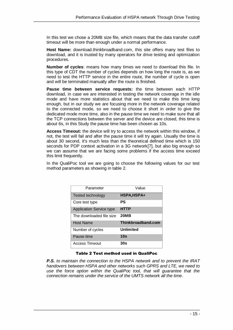
In this test we chose a 20MB size file, which means that the data transfer cutoff timeout will be more than enough under a normal performance.

Host Name: download.thinkbroadband.com, this site offers many test files to download, and it is trusted by many operators for drive testing and optimization procedures.

Number of cycles: means how many times we need to download this file. In this type of CDT the number of cycles depends on how long the route is, as we need to test the HTTP service in the entire route, the number of cycle is open and will be terminated manually after the route is finished.

Pause time between service requests: the time between each HTTP download, in case we are interested in testing the network coverage in the idle mode and have more statistics about that we need to make this time long enough, but in our study we are focusing more in the network coverage related to the connected mode, so we need to choose it short in order to give the dedicated mode more time, also in the pause time we need to make sure that all the TCP connections between the server and the device are closed, this time is about 6s, in this Study the pause time has been chosen as 10s.

Access Timeout: the device will try to access the network within this window, if not, the test will fail and after the pause time it will try again. Usually the time is about 30 second, it's much less than the theoretical defined time which is 150 seconds for PDP context activation in a 3G network‎[7], but also big enough so we can assume that we are facing some problems if the access time exceed this limit frequently.

In the QualiPoc tool we are going to choose the following values for our test method parameters as showing in table 2.

Parameter Value

Tested technology HSPA,HSPA+

Core test type PS

Application Service type HTTP

The downloaded file size 20MB

Host Name Thinkbroadband.com

Number of cycles Unlimited

Pause time 10s

Access Timeout 30s

Table 2 Test method used in QualiPoc

P.S. to maintain the connection to the HSPA network and to prevent the IRAT handovers between HSPA and other networks such GPRS and LTE, we need to use the force option within the QualiPoc tool, that will guarantee that the connection remains under the service of the UMTS network all the time.

- 16 -


3.2 Results

After setting up our data collector device (the QualiPoc device), and forming the test method, we are ready to begin the test from the starting point. After creating the Log file (the test results which contains all the signaling data between the tool and the network) we'll convert it using a conversion tool provided by ROMES, the objective of this conversion tool is to prepare the log files to be readable with the ROMES analyzer.

After that, we'll work in three basic stages:

1- Coverage Analysis 2- KPI Analysis 3- Indoor Analysis

3.2.1 HSDPA Coverage Analysis

To define the UMTS coverage area we need to define how should the network and the user equipment (UE) behave within the "covered" area, for example, can we consider an area with extremely low data rate or an area with bad retainability where drop calls occurred repeatedly as a covered area? Or we can just define the coverage in the means of the accessibility? In fact the three UMTS network phases (Accessibility, retainability and mobility) are effected by mainly two parameters, the Received Signal Code Power (RSCP) and Ec/Io which is the energy per chip over the interference (the level of interference + the noise level). Operators tend to define the coverage area as the geographical area where certain services must be available for the subscribers; we can redefine this definition technically to be the coverage area is the geographical area where a certain level of RSCP and Ec/Io must be provided. In the following we are going to discuss some metrics which will help us to evaluate the network coverage in the studied area.

3.2.1.1 Cell Analysis

The purpose of this analysis is to identify which frequencies and SCs have been used to cover the studied area, which helps to determine some problems as missing neighbors or interference issues (in frequency or code level).

The Campus Nord is served (in the outdoor) by two UL/DL ARFCNs (at the time of the test) from one band (the 2100 band) as shown in the table 3.

Band Name UARFCN

DL Downlink

[MHz] UARFCN

UL Uplink [MHz]

1 2100 10838 2167.6 9888 1977.6

1 2100 10813 2162.6 9863 1972.6

Table 3 UL/DL ARFCN covering Campus Nord

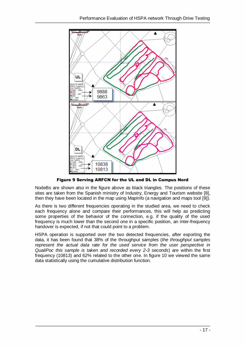
Figure 9 shows the operational channel (ARFCN) through which HSPA connections are handled across the test locations in the Campus Nord for the UL and the DL.

- 17 -


Figure 9 Serving ARFCN for the UL and DL in Campus Nord

NodeBs are shown also in the figure above as black triangles. The positions of these sites are taken from the Spanish ministry of Industry, Energy and Tourism website ‎[8], then they have been located in the map using MapInfo (a navigation and maps tool ‎[9]).

As there is two different frequencies operating in the studied area, we need to check each frequency alone and compare their performances, this will help as predicting some properties of the behavior of the connection, e.g. if the quality of the used frequency is much lower than the second one in a specific position, an inter-frequency handover is expected, if not that could point to a problem.

HSPA operation is supported over the two detected frequencies, after exporting the data, it has been found that 38% of the throughput samples (the throughput samples represent the actual data rate for the used service from the user perspective in QualiPoc this sample is taken and recorded every 2-3 seconds) are within the first frequency (10813) and 62% related to the other one. In figure 10 we viewed the same data statistically using the cumulative distribution function.

- 18 -


Figure 10 CDF for the RSCP data

From figure 10 we can notice that the data for the frequency 10813 almost has a normal distribution (x (0.5) = -74 which is equal to the data average) and with a standard deviation = 8, which means that most of the data is located between [-82, -66] dBm.

Also figure 11 shows the CDF function for the Ec/Io data.

Figure 11 CDF for Ec/Io

The number of samples in the case of Ec/Io is the same as in the RSCP case; also the distribution of the samples among both of the frequencies 40% for 10813 and 60% for 10838. When calculating the average, the UARFCN 10813 wins by 1 dB, table 4 compare the UARFCNs in the studied terms taking only the averages.

Throughput [Kbit/s] RSCP [dBm] Ec/Io [dB]

UARFCN: 10813 4610 -74 -11.9

UARFCN: 10838 3591 -82 -12.9

Table 4 Comparing URFCN in Campus Nord

0

0,1

0,2

0,3

0,4

0,5

0,6

0,7

0,8

0,9

1

-41,0 -31,0 -21,0 -11,0 -1,0

Ec/Io

CDF-10813

CDF-10838

- 19 -


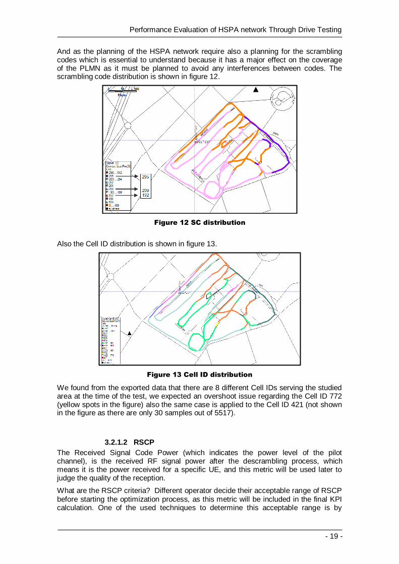
And as the planning of the HSPA network require also a planning for the scrambling codes which is essential to understand because it has a major effect on the coverage of the PLMN as it must be planned to avoid any interferences between codes. The scrambling code distribution is shown in figure 12.

Figure 12 SC distribution

Also the Cell ID distribution is shown in figure 13.

Figure 13 Cell ID distribution

We found from the exported data that there are 8 different Cell IDs serving the studied area at the time of the test, we expected an overshoot issue regarding the Cell ID 772 (yellow spots in the figure) also the same case is applied to the Cell ID 421 (not shown in the figure as there are only 30 samples out of 5517).

3.2.1.2 RSCP

The Received Signal Code Power (which indicates the power level of the pilot channel), is the received RF signal power after the descrambling process, which means it is the power received for a specific UE, and this metric will be used later to judge the quality of the reception.

What are the RSCP criteria? Different operator decide their acceptable range of RSCP before starting the optimization process, as this metric will be included in the final KPI calculation. One of the used techniques to determine this acceptable range is by

- 20 -


checking the quality of the service under different RSCP with the isolation from (as possible) the other metrics, for example, the RSCP criteria could be divided based on the Throughput. Typically we can see that the acceptable RSCP value is between -90dBm and -100dBm.

In this study we'll calculate the average RSCP in the studied area as a first step, after that we need to locate the weak RSCP spots, the key of deciding whether this spot is bad or good in terms of RSCP is how the connection between the device and the network will be handled in these spots, by surveying the area using QualiPoc and comparing some of the most known HSPA metrics to each other as in the analyzing below.

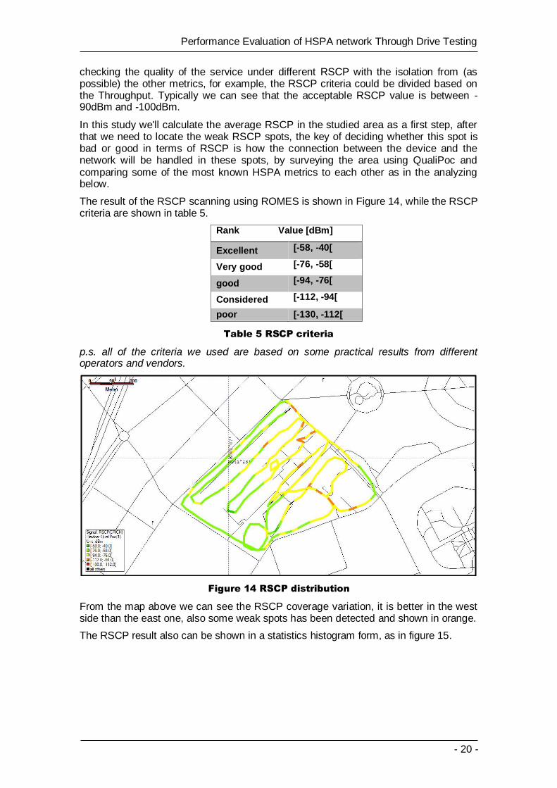
The result of the RSCP scanning using ROMES is shown in Figure 14, while the RSCP criteria are shown in table 5.

Rank Value [dBm]

Excellent [-58, -40[

Very good [-76, -58[

good [-94, -76[

Considered [-112, -94[

poor [-130, -112[

Table 5 RSCP criteria

p.s. all of the criteria we used are based on some practical results from different operators and vendors.

Figure 14 RSCP distribution

From the map above we can see the RSCP coverage variation, it is better in the west side than the east one, also some weak spots has been detected and shown in orange.

The RSCP result also can be shown in a statistics histogram form, as in figure 15.

- 21 -


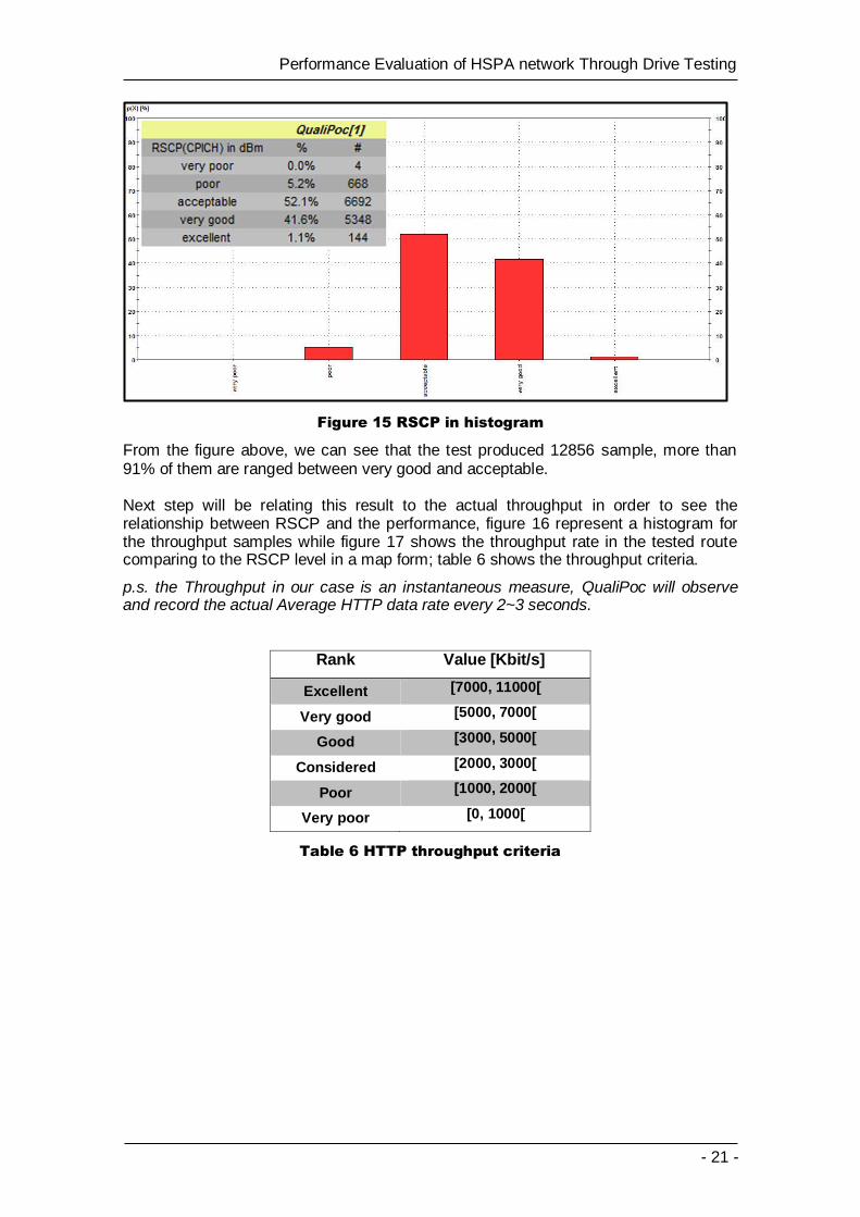
Figure 15 RSCP in histogram

From the figure above, we can see that the test produced 12856 sample, more than 91% of them are ranged between very good and acceptable. Next step will be relating this result to the actual throughput in order to see the relationship between RSCP and the performance, figure 16 represent a histogram for the throughput samples while figure 17 shows the throughput rate in the tested route comparing to the RSCP level in a map form; table 6 shows the throughput criteria.

p.s. the Throughput in our case is an instantaneous measure, QualiPoc will observe and record the actual Average HTTP data rate every 2~3 seconds.

Rank Value [Kbit/s]

Excellent [7000, 11000[

Very good [5000, 7000[

Good [3000, 5000[

Considered [2000, 3000[

Poor [1000, 2000[

Very poor [0, 1000[

Table 6 HTTP throughput criteria

- 22 -


Figure 16 throughput Histogram

Figure 17 RSCP vs. throughput

As we can see in figure 17, there is an obvious relation between the bad RSCP spots and the throughput rate, clearly the data rate decreases when the RSCP level goes down, for more precise view for this result see figure 18, which represent the RSCP criteria with the average throughput level in a 2D chart.

- 23 -


Figure 18 RSCP vs. average throughput

From the figure above we can find that the relation between the throughput and the RSCP level is a positive relation, and when the received signal level is poor (between -130 and -112) the average is 1909 Kbit/s, while it reaches to 6535 Kbit/s in the excellent criteria (between -58 and -40).

From the figure above we can see that the RSCP value affects the throughput rate but yet it is not the only factor as this parameter only includes the path loss between the NodeB and the device which is not completely enough to evaluate the throughput.

3.2.1.3 CPICH Ec/Io

This ratio is similar to the SNR in other telecommunication systems; it is the ratio between the received energy per chip and the interference level in addition to the noise level regarding the PICH, in case there is absolutely no interference, this ratio will be seen as SNR. So this ratio is monitored in the idle mode and used to give us a good reflection of interference and coverage problems. As for the quality of the link the metric CQI has to be analyzed and will be explained in the section 5.2.1.5 (CQI channel quality indicator).

Figure 19 shows the Ec/Io coverage as resulted from the CDT test.

Figure 19 CPICH Ec/Io distribution

1909

2836

3447

5393

6535

0

1000

2000

3000

4000

5000

6000

7000

PoorConsideredGoodVery goodExcellent

Average Throughput

- 24 -


We can see that most of the samples are within the good range as we can see in figure 20 which shows a histogram for the Ec/Io distribution; there are some red (poor) samples seen in figure 19, usually as these samples are short in time the network will not take a decision as the trigger window is bigger.

Figure 20 CPICH Ec/Io histogram

Figure 21 shows the relation between RSCP and the CPICH Ec/Io in a scatter plot.

Figure 21 Ec/Io Vs RSCP

We can see from the figure above that almost all the samples are located between RSCP: [-50, -100] dBm and Ec/Io: [-4, -30] dB.

0

1000

2000

3000

4000

5000

6000

7000

8000

ExcellentVery GoodGoodConsideredPoor

Excellent

Very Good

Good

Considered

Poor

-50

-40

-30

-20

-10

0

-120 -110 -100 -90 -80 -70 -60 -50 -40 -30

CPICH EcIo Vs RSCP

- 25 -


Also, in the following figure 22, we can see the relation between the throughput and the Ec/Io, also shown in a scatter plot.

Figure 22 Ec/Io Vs TP

To combine the RSCP and the Ec/Io or in other words the path loss and the interference in one figure we need to have a look into the RSSI.

3.2.1.4 RSSI

The Received Signal Strength Indicator, it combines the RSCP and the Ec/Io in one figure as the equation:

RSSI [dBm] = RSCP [dBm] - Ec/Io [dB]

Figure 23 shows the RSSI coverage as resulted from the CDT test.

Figure 23 RSSI distribution

Figure 24 illustrate the RSCP, Ec/Io and the RSSI in one plot, the Ec/Io as the x-axis. We can see that the RSSI have a minimum value near -88 dBm, this value can be considered as the receiver sensitivity ‎[10] (our test device) which mean that the minimum power require to receive the signal form the NodeB and process it is

-45

-40

-35

-30

-25

-20

-15

-10

-5

0

0200040006000800010000

Ec/Io Vs TP

- 26 -


RSSI= -88 dBm (for the specific test device) but yet this value could be not accurate as the studied area is small.

Figure 24 Ec/Io, RSCP and RSSI

As a result we can see that the coverage within Campus Nord is good in the terms of the received signal strength and quality and that is expected as the NodeBs are near to the studied site, but still the average throughput for the whole area is about 4000 Kbit/s which is much less than the HSDPA theoretical rate (about 14000 Kbit/s). So further investigation about the throughput will be done later under the section 5.2.3.4.1 (Service integrity: HSDPA User Throughput).

3.2.1.5 CQI (Channel Quality Indicator)

It is a measurement of the radio channel condition that is aimed to indicate which the estimated transport block size (TBS), modulation type and number of parallel codes could be received correctly with a BLER no greater than 10% in the downlink direction.

The CPICH Ec/Io measurements collected during HSDPA Transmission could mask the true radio conditions, because while the HSDPA session adds to the overall load of the cell which is taken into consideration during the computation of Ec/Io, this computation does not necessarily give the TRUE radio conditions. So as an alternative to the Ec/Io in High Speed Sessions the parameter CQI was added to give the true radio conditions to be reported to the NodeB.

The following example is to explain why the Ec/Io computations in HS session do not necessarily give the true radio conditions: As we know, HSDPA uses the remaining power of the cell after power is allocated to the common channels and dedicated channels as shown in figure 25.

-100

-90

-80

-70

-60

-50

-40

-30

-20

-10

0

-1,6

-4,4

-4,8

-5,2

-5,4

-5,7

-5,9

-6,1

-6,3

-6,5

-6,7

-6,9-7

-7,2

-7,5

-7,7

-7,9

-8,1

-8,3

-8,6

-8,8

-9,1

-9,3

-9,5

-9,7

RSCP

RSSI

- 27 -


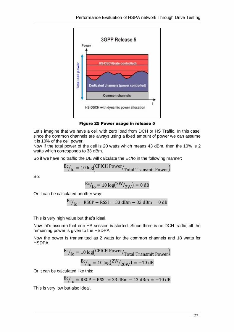
Figure 25 Power usage in release 5

Let’s imagine that we have a cell with zero load from DCH or HS Traffic. In this case, since the common channels are always using a fixed amount of power we can assume it is 10% of the cell power. Now if the total power of the cell is 20 watts which means 43 dBm, then the 10% is 2 watts which corresponds to 33 dBm.

So if we have no traffic the UE will calculate the Ec/Io in the following manner:

⁄ (

⁄ )

So:

⁄ ( ⁄ )

Or it can be calculated another way:

⁄

This is very high value but that’s ideal.

Now let’s assume that one HS session is started. Since there is no DCH traffic, all the remaining power is given to the HSDPA.

Now the power is transmitted as 2 watts for the common channels and 18 watts for HSDPA.

⁄ (

⁄ )

⁄ ( ⁄ )

Or it can be calculated like this:

⁄

This is very low but also ideal.

- 28 -


From this calculations we can say that In Idle mode and with no resources allocated, a UE will measure as low as 0 dB Ec/Io and in HS Mode and with no resources allocated on DCH, a UE will measure as low as -10dB. It cannot report any better than -10dB.

That means, in a live network where resources of a cell are shared between many users, and Interference from other cells also plays its part, the Ec/Io will always give a FALSE value for an HSDPA user. And it will show a very poor value. And that’s why we use CQI.

HSDPA utilizes link adaptation techniques to substitute power-control and variable spreading factor. This link-adaptation algorithm that is managed by the Node-B is very dynamic and adjusts the transmit bit rate on the HS-DSCH every 2-ms TTI.

While SINR is used to evaluate the channel quality as observed by the receiver, the UE calculate the CQI value to be reported to the NodeB via a linear mapping as shown below:

[ ]

The UE periodically sends a CQI to the serving HS-DSCH cell on the uplink high-speed dedicated physical control channel (HS-DPCCH). These CQI values are used by the link adaptation algorithm at the Node-B so that every CQI value reported corresponds to the Transport Block Size (TBS) that can be granted on a particular Modulation type and Number of codes (CQI to TBS mapping tables).

The HSDPA system defines a different CQI mapping table for different categories of UEs. The category is determined according to the capability of UE.

So the system (NodeB) is essentially calculating the Data Rate to be scheduled to the user based on CQI reports and BLER which it receives from the UE, as shown in figure 26.

[ ] [ ]

[ ]⁄

Figure 26 Data rate calculation procedure in HSDPA

Note that large CQI numbers denote a good channel quality and a high potential DL data throughput. In our case study we first captured the CQI distribution in Campus Nord as shown in figure 27, then we analyzed the CQI values reported by the mobile and it appears to us from the figure 28 below that the mobile experienced in average good quality values which correspond to an average value of 22.3 for the CQI. And

- 29 -


also in about 94 % of the time during the drive test the CQI values were between 20 and 30.

Figure 27 CQI distribution in campus Nord

Figure 28 CQI Statistics

The figure 29 below shows the relation between Ec/Io and CQI. We can see that Ec/Io doesn’t give a view on the true radio channel quality as we find high CQI values and low Ec/Io value and as explained before, CQI is the true indicator of the channel condition in the case of HSDPA transmission.

- 30 -


Figure 29 CQI Vs Ec/Io

Figure 30 below shows the relation between CQI and the throughput achieved. As mentioned before, high CQI values lead to high potential throughput and we can see from the figure that the highest data rates achieved (above 9000 Kbps) when we had a very good CQI values, however as we can see from the figure there are low data rates corresponding to high CQI values. We conclude from this that high CQI values do not necessarily provide high data rates because there are other factors that affects the throughput and to achieve high data rates the CQI value must be high. Further investigation about throughput and CQI can be found later in the section (Error! Reference source not found. Error! Reference source not found.)

Figure 30 CQI Vs Throughput

To see the relation between the CQI and the RSCP, the figure 31 below shows a plot for CQI Vs RSCP and we can note that as the RSCP level gets higher, the CQI tends

0

5

10

15

20

25

30

-45 -40 -35 -30 -25 -20 -15 -10 -5 0

CQ

I

Ec/Io [dBm]

0

5

10

15

20

25

30

0,00 2000,00 4000,00 6000,00 8000,00 10000,00 12000,00

CQ

I

Throughput [Kbps]

- 31 -


to get higher. Also we can see some dropping in the CQI values even when we have high RSCP level and that’s probably due to the interference as the CQI is directly related to the Signal to interference and noise ratio (SINR).

Figure 31 CQI Vs RSCP

3.2.2 KPI Analysis (HSDPA)

In this section we evaluated some of the main and most use KPIs in the UMTS networks, the KPIs ordering is based on its categories (Accessibility, Retainability, Mobility and Quality of Service KPIs)

3.2.2.1 Accessibility KPIs Analysis

The RAB establishment success rate and the PDP context activation success rate are important KPIs because they allow us to measure the accessibility across the radio access network UTRAN. In other words, the importance of these KPIs comes from the fact that they show us how easy it is for the user to obtain a service within specified tolerances and other given conditions.

3.2.2.1.1 RAB Establishment Success Rate (RABESR)

From the equation above we can notice that this KPI is the percentage of how many RABs have been established successfully in the packet switched domain, and is calculated by analyzing the layer 3 messages and then filtering the data to get the required messages to get the count of the number of attempts and successful RAB establishments. In our case this percentage appears to have a perfect value indicating that all of the RAB establishments were successful.

0

5

10

15

20

25

30

-120 -110 -100 -90 -80 -70 -60 -50 -40

CQ

I

RSCP [dBm]

- 32 -


3.2.2.1.2 UMTS PDP Context Activation Success Rate (UPDPCASR)

From the equation above we can notice that this KPI is the percentage of how many PDP context activation procedures have been established successfully, and is calculated by analyzing the layer 3 messages and doing some filtering and processing to get the count of the number of attempts and successful RAB establishments. In our case we have only one attempt of PDP context activation procedures initiated by MS because in this test we have a single RAB service and that means we have one PDP context to be established and the result was successful.

3.2.2.1.3 HSDPA call setup time

HSDPA call setup time indicates Network response time to a user request for a HSDPA data service. The call setup time is an important KPI as high and unusual call setup time could be an indicator to some access problems. The typical values of HSDPA call setup time are between [0.5-1] second ‎[11].

HSDPA call setup time can be calculated from observing the layer 3 messages and it is defined as the difference in time between the “RRC Connection request” message and the “PDP Context Activation Accept” message. Figure 32 below shows an HSDPA call procedure in the layer 3 level.

Figure 32 Call Setup Time procedure

And figure 33 below shows the corresponding messages in ROMES.

- 33 -


Figure 33 L3 messages for CST in ROMES

Analyzing the call setup time in our case study, we find a value of 2.45 seconds. And we clearly see that this value is more than it should be according to the typical values in HSDPA network however in order to evaluate the response time, more than one test of call setup must be done and this value that we have is only one sample and evaluating the response time on one sample is not enough.

3.2.2.2 Retainability KPIs analysis

RAB abnormal release rate is important to be calculated because it shows us the ability of the RAB to be kept, once it is established under given conditions until its normal release.

3.2.2.2.1 RAB Abnormal Release Rate (RARR) or PS Service Drop Ratio

This KPI is calculated by observing the layer 3 messages, and it is defined as the ratio of the number of RAB release requests divided by the number of successful RAB establishments.

The purpose of the RAB Release Request procedure is to enable UTRAN to request the release of one or several radio access bearers. This message is triggered by the RNC and the reason behind it is for example due to RF reasons (Failure in the Radio interface procedure, signaling RLC reset or traffic RLC reset) or due to abnormal reasons (Cell congestion, UTRAN generated reason, OM intervention and so on).

In our case the RAB assignments are behaving in a very good way and no abnormal RAB releases were found.

- 34 -


3.2.2.3 Mobility KPIs Analysis ‎[12]

3.2.2.3.1 Soft Handover Success Rate (SHOSR)

In HSDPA, the HS-DSCH for a given UE belongs to only one of the radio links assigned to the UE (the serving HS-DSCH cell), but the UE uses Soft Handover for the Uplink and the Downlink DCCH and not for the HS-DSCH using the existing triggers and procedures for the active set update (Event 1A, 1B, 1C).

The Soft Handover rate in traffic statistics indexes is over high. Usually more than two cells exist in the active set most of the time during the drive test, and they are in SHO state. This KPI is important because using SHO decreases the UL interference. Below you will find the equation for calculating the soft handover success ratio which will be seen in the next step that it is the ratio of the number of “Active set update complete” (L3 messages) to the number of “Active set update” (L3 messages).

The reference value for this ratio is to be above 96% (this value could slightly differ from operator to another).

During the drive test, all the active set update attempts were completed successfully.

In the figure 34 below, you can find a sample of updating the active set and adding a cell to be in the soft handover mode. In this figure you can see the measurement report sent by the UE in the uplink triggered by the event 1A to indicate that a primary CPICH enters the reporting range and must be added to the active set in soft handover mode according to the measurement result on the its signal quality (SC number 200 in this case enters the reporting range).

Then the NodeB sends the a command to the UE to perform the soft handover by sending an Active set update message (shown with its main details in the figure 35), in this message you can see mainly the indication of the primary scrambling code to be added to the active set according on the measurements result received before.

The UE once it completes this procedure, it sends an “active set update complete” message to the network to indicate that it is done successfully.

- 35 -


Figure 34 Measurement report (Event 1A)

Figure 35 Active set Update message

- 36 -


3.2.2.3.2 Change of Serving HS-DSCH Cell Success Rate (CSCSR)

As mentioned before, in HSDPA, Changing the serving HS-DSCH cell is not supported in Soft handover but it must be a Hard Handover because of complexity issues.

This intra-frequency hard handover is triggered by the event 1D in the measurement report sent by the UE to the network and it is also important because the failure in this handover will lead to drop calls. It happens when the UE changes the serving cell in the active set on the same frequency with no micro-diversity involved. The process and the functionality of this handover involve some of RRC procedures like “Physical channel reconfiguration”.

Intra-frequency hard handover attempts were perfectly successful and we conclude from this that changing the serving cell behavior was very good.

In the figure 36 below, you can find a sample of changing the serving cell procedure in the layer 3 messages taken from ROMES. You can see in this figure that first the UE sends a measurement report to the network triggered by the event 1D, this event means that a change of the best cell must be done according to the measurement results contained in this report that shows in this case that the signal quality (CPICH-Ec/No and CPICH-RSCP) received from the primary scrambling code number 200 is better than the currently serving scrambling code 192.

Figure 36 Measurement report (Event 1D)

After that in the figure 37, you can see the command that is sent by the NodeB to the UE (physical channel reconfiguration message) based on the measurement results received before, mainly in the details of this command you can see the indication of the new serving cell that must be tuned to (SC number 200 in this case) and also you can see the indication of cancelling the previous serving cell (SC 192).

- 37 -


Once this command is received by the UE, it changes its serving cell according to the details included in this message and after completing this procedure, the UE sends “physical channel reconfiguration complete” to indicate to the network that changing the serving cell is done successfully.

Figure 37 Changing the serving cell command

3.2.2.4 QoS KPIs Analysis

3.2.2.4.1 Service integrity (User Throughput HSDPA)

This KPI is very important because it indicates the Downlink Average Packet data throughput (kbps) for the HSDPA user. The figure below shows the result of the data rates achieved during the drive test.

Average throughput = 4290 Kbps.

Maximum throughput reached = 10113 Kbps.

Figure 38 shows the distribution of the throughput samples based on specific category as shown in the same figure.

- 38 -


Figure 38 Throughput distribution

In the figure 39 shows the same distribution but in a map view across the Campus Nord. We can clearly see that the eastern part of the campus has good values of throughput due to good radio quality conditions in that part, while on the other hand we have western part that shows us poor values of throughput due to poor radio quality conditions.

Figure 39 TP distribution within Campus Nord

To further evaluate the performance regarding the throughput, additional investigation will be done by comparing the throughput achieved with several metrics like CQI and BLER.

3.2.2.4.1.1 CQI Vs Throughput

To analyze the relation between the CQI and throughput achieved in the test, we categorized the throughput range of values into 3 categories:

• Good throughput values range: [4000-10800] Kbps.

• Considered throughput values range: [2000-4000] Kbps.

• Poor throughput values range: [0-2000] Kbps.

- 39 -


When analyzing the values of the CQI samples that correspond to good average throughput value we can see also in most of the times that we have higher values compared to the CQI samples that correspond to Poor average throughput value, and this makes sense because we know that good CQI value leads to a potential high throughput value. On the other hand also we can see from figure 40 below that sometimes we have high CQI value but LOW throughput is achieved and this also makes good sense because the data rates achieved depend not only on the reported CQI values but also depends on the BLER. And this low throughput values are due to high BLER values.

Note that the X-axis is the samples taken and the Y-Axis is the CQI range of values from 0 to 30.

Figure 40 CQI Vs Throughput

3.2.2.4.1.2 DL BLER VS Throughput Analysis

Block error rate (BLER) is an analysis of transmission errors on the radio interface and it is based on analysis of cyclic redundancy check (CRC) results for radio link control (RLC) transport blocks and computed by defining the relation between the numbers of RLC transport blocks with CRC error indication and the total number of transmitted transport blocks as expressed in Equation below:

[ ] ∑

∑

Analyzing the DL BLER relation with throughput gives a good insight about how the interference degrades the throughput. We can see from the figure below a comparison between the values of the BLER while a high data rates are achieved on one hand and on the other the values of BLER while a poor data rates are achieved. We can notice that we have very low BLER ratios while achieving high data rates and we have much higher BLER with the poor throughput, it makes absolutely sense because higher BLER leads to more packet retransmissions, which increases the delay. Long delays imply that TCP will send at a bit rate lower than the maximal bit rate of the radio link for long periods of time. So because of interference we get higher BLER which leads to a lower data rates. See the figure below and note that the X-axis is the samples taken and the Y-axis is the values of the DL BLER [%].

0

5

10

15

20

25

30

35

1 5 9

13 17 21 25 29 33 37 41 45 49 53 57 61 65 69 73 77 81 85 89 93 97

101

CQI Samples with GOODAverage ThroughputCQI Samples with BADAverage Throughput

- 40 -


Figure 41 BLER Vs Throughput

3.2.2.4.2 Number of HS-DSCH codes

This KPI indicates how much High Speed- Download Shared Channel Codes dedicated to the HSDPA user during the drive test, figure 42 below shows the number of the codes used in this test.

Figure 42 number of channelization codes statistics

In the figure 43 below you can see the relation between the data rates achieved in HSDPA and the number of HS-DSCH codes given to the user. The figure shows us clearly that when the user gets more codes it can achieve higher data rates. We can see also from the figure that even in the range of the poor throughput values we have good number of channelization codes given to the user so we can conclude from that the reason behind the poor throughput is not the lack of channelization codes (high load case) but instead the interference that leads to this kind of poor values.

Note that the X-axis is the samples taken and the Y-Axis is the number of codes from 0 to 15.

0

5

10

15

20

25

30

35

40

45

1 3 5 7 9 11 13 15 17 19 21 23 25 27 29 31 33 35

BLER in the range of GOODthroughput valuesBLER in the range of Poor throughputvalues

- 41 -


Figure 43 # of codes during good Throughput

As the Throughput is the most important parameter in HSDPA, and after analyzing the

main metrics that contribute in the throughput achieved, we saw that during the test,

considerably high throughputs were achieved given a good radio conditions( Good CQI

values) in most of the test. However there are some periods when the UE suffered from

a relatively bad radio conditions or high interference which led to very poor throughputs

that affected the overall average throughput value that we saw in this analysis.

In table 7 below you can see the overall result of the HSDPA KPI analysis.

KPI Category Reference

value Count Calculated Value

RABESR Accessibility 99% ‎[13]‎[13] Att.=113

Succ.=113 100%

UPDPCASR Accessibility 99% ‎[13] Att.=1

Succ.=1 100%

RARR Retainability <2% ‎[14] Att.=0 0%

SHOSR Mobility 96% ‎[13] Att.=173

Succ.=173 100%

CSCSR Mobility 99% ‎[13] Att.=180

Succ.=180 100%

Throughput Service Integrity

----- -----

In Average =4.290 Mbps

Max =10.113 Mbps

#HS-DSCH codes

QoS ----- ----- Average =11.2 Codes

Call Setup Time

Latency [0.5-1]

seconds ‎[11]‎[11] ----- 2.450 s

DL BLER Service Integrity

10% ----- In Average =1.5%

Maximum

0

2

4

6

8

10

12

14

1 4 7 101316192225283134374043464952555861646770737679828588919497

#Codes in the range of Good Throughput values#Codes in the range of Poor Throughput Values

- 42 -


reached=42%

Table 7 HSDPA KPIs

3.2.3 HSUPA Coverage Analysis

To perform an HSUPA we used the same test method as in the HSDPA case, but modified a little bit so the device will be uploading instead of downloading, table 8 shows the test method that we used in QualiPoc to check the HSUPA coverage analysis.

Parameter Value


Core test type PS



The uploaded file size 90MB

UL host name Directlinkupload.com

Pause time 10s

Access Timeout 30s

Table 8 HSUPA test method

3.2.3.1 RSCP Analysis

We can follow the same criteria for the RSCP parameter to extract an analysis result for the coverage in HSUPA. Even though RSCP is a pure coverage indicator on downlink, but it can be used also in uplink with reasonable accuracy.

Figure 44 shows the RSCP distribution in the studied area in campus Nord.

Figure 44 RSCP distribution in HSUPA

- 43 -


In the figure 45 below you can find the RSCP statistics in the test:

Figure 45 RSCP Statistics

RSCP statistics shows us that about 92% of the RSCP samples taken were between [-85 to -105 dBm]. When analyzing the throughput values and taking into account the RSCP values, the result can be summarized in the following table:

RSCP Range [dBm] HSUPA average

Throughput [Kbit/s]

[-80 to -90] 549

[-90 to -100] 537

[-101 to -120] 348

Table 9 HSUPA average throughput Vs RSCP

From this table we can see that mainly as the RSCP level is degrading, the HSUPA throughput in average is also degrading and from that we can say that RSCP generally gives us a considered indication about the coverage and performance in the uplink direction. In the figure 46 below you can see the throughput values versus the corresponding RSCP values. Also note that the throughput samples and their corresponding RSCP samples are not taken continuously in time but taken in different times, and are used in this figure to compute the average throughput values in each RSCP range and compare between them which allowed us to conduct a relation between the RSCP and the HSUPA throughput.

- 44 -


Figure 46 HSUPA throughput VS RSCP

3.2.3.2 TX Power Analysis

The TX power of the UE is an indicator of the coverage. The UE uses the power control mechanism to compensate the losses of the link in order to reach the NodeB with a certain level determined by the network. By knowing that, we can say that by moving away from the cell (the coverage decreasing), then the UE needs to use higher transmit power in order to compensate the losses. This we lead us to define criteria for the TX power as shown in table 10.

Table 10 TX power Criteria

0

200

400

600

800

1000

1200

1400

1600

-80,

6

-84,

1

-85,

5

-87,

5

-90

-90,

3

-90,

7

-90,

9

-91,

3

-91,

6

-91,

9

-92,

5

-92,

9

-93,

6

-94

-94,

4

-95

-95,

5

-95,

8

-96,

4

-97,

1

-97,

6

-98,

5

-98,

9

-99,

7

-10

0,7

-10

1,7

-10

2,8

-10

4,3

-10

6,1

-11

2,8

HSUPA InstantaneousthroughputThroughput average value

Coverage Value [dBm]

Excellent [-40, -10[

Very good [-10, 0[

good [0, 10[

Considered [10, 15[

poor [15, 20[

- 45 -


The distribution of the TX power values in the studied area in campus Nord is shown in figure 47.

Figure 47 Tx power distribution in HSUPA

The figure 48 below shows the relation between the TX power of the UE and the RSCP. We can see that in general in the range of low RSCP level, the TX power has mostly high values and on the other hand we see in the range of higher RSCP level the TX power has lower values. This demonstrates how the TX power of the UE is used to indicate the status of the coverage.

For the duration of the entire test the average TX power was 10.5 dBm indicating a coverage that is between acceptable and a bit poor.

Figure 48 TX Power Vs RSCP

-15

-10

-5

0

5

10

15

20

25

-120 -115 -110 -105 -100 -95 -90 -85 -80 -75 -70

TX P

ow

er [

dB

m]

RSCP [dBm]

- 46 -


3.2.3.3 UL interference

The UL interference is a very important element in the HSUPA, because in HSUPA the shared resource is the amount of allowed uplink interference which depends on transmission power of the UEs. And so the scheduler in this case needs to control the UL interference by controlling the amount of power expected from each UE that will use the power control mechanism to reach the base station at that certain amount of power.

Controlling the power expected from the UE at the NodeB (by controlling the Serving grants given to the UE) means controlling the data rate that can be achieved by that UE.

High data rates means high transmission power from the UEs and that means high interference and so the scheduler has to manage that by putting a restriction on the serving grants given to the users so that intra cell interference is not too high and the UL transmission can be received properly. However restrictions come not from only intra-cell interference but also from the neighboring cells that will also will command the UE in soft handover to lower its transmission power (and so lowering the data rate) if the inter-cell interference is high.

In the figure below you can see the relation between the UL interference and the throughput achieved. We can note clearly that the throughput gets lower as the UL interference gets higher.

In other words, the restriction on the power given to the user to be used (restrictions on Serving grants due to high UL interference) is limiting the average throughput.

Figure 49 Throughput Vs Uplink Interference

0

200

400

600

800

1000

1200

1400

1600

-104 -103 -102 -101 -100 -99 -98 -97 -96

UL

Thro

ugh

pu

t [K

bp

s]

UL Interference [dBm]

- 47 -


3.2.4 KPI analysis (HSUPA)

3.2.4.1 Accessibility KPIs analysis

The accessibility KPIs for the HSUPA network can be calculated in the same manner as we did in the HSDPA because clearly the accessibility functions are the same.

3.2.4.1.1 RAB Establishment Success Rate (RABESR)

In this case also, after doing the processing of the layer 3 messages and counting the establishment attempted and succeeded, the result percentage was 100% successful.

3.2.4.1.2 UMTS PDP Context Activation Success Rate (UPDPCASR)

As mentioned before, since we have only a single RAB test, we had only one PDP context activation request and also it was successful.

3.2.4.2 Retainability KPI analysis

3.2.4.2.1 HSUPA Service drop rate or RAB Abnormal Release Rate (RARR)

From observing the layer 3 messages, the UE didn’t encounter any abnormal release of service and so all the RABs established were maintained successfully until normal release.

3.2.4.3 Mobility KPIs analysis ‎[15]

3.2.4.3.1 Change of Serving Radio Link Set success ratio (CSRLSSR)

In HSUPA the UE uses soft handover for associated DCH as well as for E-DCH Using existing triggers and procedures for the active set update (events 1A, 1B, 1C). The importance of this KPI comes from the fact that using the soft handover will prevent the interruption in the transmission of data and also because it will reduce the uplink interference and so will increase the capacity of the system. Below you will find the equation for calculating the Change of Serving Radio Link Set success ratio which in fact is the ratio of the number of “Active set update complete” layer 3 messages to the number of “Active set update” messages.

The soft handover success ratio was very good in the tested route.

3.2.4.3.2 Change of serving E-DCH cell success rate (CSCSR)

The UE receives Access Grants on E-AGCH from only one cell out of the E-DCH active set (serving E-DCH cell) and since E-DCH and HSDPA serving cell must be the same, this change can be a Hard Handover using RRC procedures and triggered by event 1D.

- 48 -


Note also that this change of serving cell in HSUPA could be combined with Active Set Update procedure. This hard handover is important because the failure in this handover will lead to drop calls.

This KPI can be calculated from the layer 3 messages and it is the ratio of the number of “physical channel reconfiguration complete” messages to the number of “physical channel reconfiguration” messages as shown in the equation below:

After calculating the ratio, the resulted percentage was 100% of successful attempts of changing the serving E-DCH.

3.2.4.4 QoS KPIs analysis

3.2.4.4.1 Service Integrity (HSUPA User Throughput)

This KPI indicates the Uplink Average Packet data throughput (kbps) for the HSUPA user. In the figure 50 below shows the result of the data rates achieved during the drive test.

The theoretical maximum throughputs on the uplink are 5.74 Mbps (for a TTI =2ms and with 2 SF4 and 2 SF2 codes) and 2 Mbps (for a TTI=10ms and with 2 SF4) for our UE’s category (category 6), however in practical, maximum throughput could only be achieved with near perfect conditions and by giving the vast majority, if not all, of the capacity to one user which is very unlikely to happen.

In our test, the values achieved are:

Average throughput was around 500 Kbps.

Maximum throughput reached = 1.448 Mbps.

Figure 50 HSUPA Throughput

The reason behind this limitation of the practical throughputs achieved in HSUPA is due to 3 types of limitations:

Limitation by Serving Grants (SG): due to restrictions on the UL interference level.

- 49 -


Limitation by Transmission Power: when the mobile is using the max power to transmit.

Limitation by the scheduled Data to be sent: when the UE is not able to transmit all the scheduled data allowed by SG.

To see the serving grants values, in the figure below you can see a CDF plot of the Serving Grants given to the user during the test. We can see that 50% of serving grants indexes given were below 20. We note also that the range of the SG is [0- 31].

Figure 51 Mean Serving Grants

In the figures 52, 53 and 54 below you can find the percentages of these 3 limitations during the test:

Limited by Serving Grants (SG)

Figure 52 SG limitation

0

0,1

0,2

0,3

0,4

0,5

0,6

0,7

0,8

0,9

1

0 2 4 6 8 10 12 14 16 18 20 22 24 26 28 30

Act

ual

Fre

qu

en

cy

Serving Grant Index

- 50 -


Limited by Maximum Power

Figure 53 Power limitation

Limited by scheduled data

Figure 54 Scheduled data limitation

We conclude from these figures that the throughput in about 65% of test period was limited in a percentage between [75-100%] due to restriction on UL interference. And in 90% of the test period the UE was limited in a percentage less than only 10% due to the maximum transmission power. And finally also we can see that the UE in 99% of the test period was limited in a percentage less than only 5% due to scheduled data.

- 51 -


This means the throughput was limited mostly by the restriction on UL interference because the other limitations had really small effect on the throughput. And that’s explains the low maximum throughput values achieved in practical.

3.2.4.4.2 Happy Rate

In HSUPA there is a status reporting mechanism called the happy bit. It’s a single bit that is transmitted on the E-DPCCH physical channel. It can only indicate "happy" or "unhappy" but it is sent every time the UE transmits to the network. A UE considers itself to be unhappy if it is not transmitting at maximum power and it cannot empty it’s transmit buffer with the current Serving Grant within a certain period of time. The period of time is known as the Happy Bit Delay Condition and is signaled by the RRC layer during call setup. Thus the happy bit is a crude indication of whether the UE could make good use of additional uplink power.

In the figure 55 below, we can see statistics of the Happy Rate.

Figure 55 Happy rate statistics

According to the statistics we can see that the UE was almost always “unhappy” but that also doesn’t mean that this is bad in terms of resource allocation because the scheduler needs to keep the UEs “unhappy”, otherwise more resource than necessary will need to be reserved for them.

3.2.4.4.3 BLER

In the figures 56 below we can see the relation between the BLER and UL throughput. The figure shows that as the BLER percentages get higher, the throughput achieved gets lower. That’s logical result since we know that higher BLER values mean more retransmissions and so lower data rate.

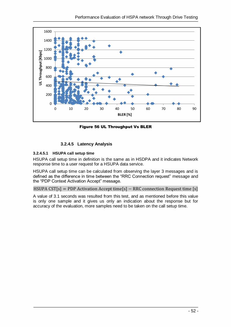
- 52 -


Figure 56 UL Throughput Vs BLER

3.2.4.5 Latency Analysis

3.2.4.5.1 HSUPA call setup time

HSUPA call setup time in definition is the same as in HSDPA and it indicates Network response time to a user request for a HSUPA data service.

HSUPA call setup time can be calculated from observing the layer 3 messages and is defined as the difference in time between the “RRC Connection request” message and the “PDP Context Activation Accept” message.

[ ] [ ] [ ]

A value of 3.1 seconds was resulted from this test, and as mentioned before this value is only one sample and it gives us only an indication about the response but for accuracy of the evaluation, more samples need to be taken on the call setup time.

0

200

400

600

800

1000

1200

1400

1600

0 10 20 30 40 50 60 70 80 90

UL

Thro

ugh

pu

t [K

bp

s]

BLER [%]

- 53 -


In the table 11 below a full summary of the HSUPA

KPI Category Reference

value Count Calculated Value

RABESR Accessibility 99% ‎[13] Att.=9

Succ.=9 100%

UPDPCASR Accessibility 99% ‎[13] Att.=1

Succ.=1 100%

RARR Retainability <2% ‎[14] Att.=0 0%

CSRLSSR Mobility 96% ‎[13] Att.=77

Succ.=77 100%

CSCSR Mobility 99% ‎[13] Att.=55

Succ.=55 100%

Throughput Service Integrity

----- -----

In Average =500 Kbps

Max =1.448 Mbps

Call Setup Time

Latency [0.5-1]

seconds‎[11] ----- 3.1 s

Table 11 HSUPA KPIs summary

3.2.5 Indoor Coverage Analysis

The indoor test was applied in two buildings, D3 and A5 as shown in figure 57 below, the target is to check the HSPA performance and the service integrity within these buildings by checking the DL and the UL throughput indoor and then compare it with the result obtained from testing the building's surrounding area.

Figure 57 Indoor building test locations

To start with the indoor test we need to prepare the tools as we did in the outdoor one, and as we do not have a sketch scheme for the buildings we won’t use the GPS nor

- 54 -


the indoor tracking mechanism that QualiPoc offers, thus the whole floor will be considered as one point where statistics and measures are changing with time. The method shown in table 12 is the one we used in QualiPoc to apply the indoor test.

Parameter Value


Core test type PS


The downloaded file size 20MB

Host Name Thinkbroadband.com


The uploaded file size 90MB

UL host name Directlinkupload.com

Pause time 10s

Access Timeout 30s

Table 12 QualiPoc Indoor test method

We applied this test method for the first three floors plus the surrounding area for each building, and then we calculated the average for RSCP, CQI, TP/DL, TP/UL, Tx power, SCCH # codes and the BLER for each floor to give a clear image regarding the Indoor coverage, then finally, we compared the Indoor values with the surrounding areas.

Building # 2 (A5)

In the figure 58 below we can see how the UARFCN frequencies and the SC are distributed within A5.

p.s. The corresponding UL ARFCNs for 3011 and 10838 are 2786 and 9888 respectively.

Figure 58 UARFCN and SC distribution in building A5

UARFCN: 10838/ SC: 192

UARFCN: 10838/ SC: 200

UARFCN: 3011/ SC: 192

UARFCN: 3011/ SC: 200

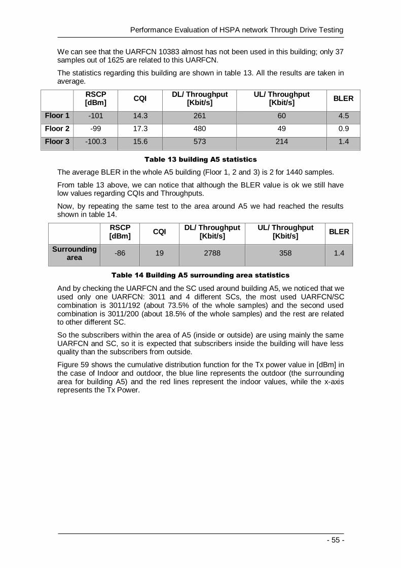
- 55 -


We can see that the UARFCN 10383 almost has not been used in this building; only 37 samples out of 1625 are related to this UARFCN.

The statistics regarding this building are shown in table 13. All the results are taken in average.

RSCP [dBm]

CQI DL/ Throughput

[Kbit/s] UL/ Throughput

[Kbit/s] BLER

Floor 1 -101 14.3 261 60 4.5

Floor 2 -99 17.3 480 49 0.9

Floor 3 -100.3 15.6 573 214 1.4

Table 13 building A5 statistics

The average BLER in the whole A5 building (Floor 1, 2 and 3) is 2 for 1440 samples.

From table 13 above, we can notice that although the BLER value is ok we still have low values regarding CQIs and Throughputs.

Now, by repeating the same test to the area around A5 we had reached the results shown in table 14.

RSCP [dBm]

CQI DL/ Throughput


[Kbit/s] BLER

Surrounding area

-86 19 2788 358 1.4

Table 14 Building A5 surrounding area statistics

And by checking the UARFCN and the SC used around building A5, we noticed that we used only one UARFCN: 3011 and 4 different SCs, the most used UARFCN/SC combination is 3011/192 (about 73.5% of the whole samples) and the second used combination is 3011/200 (about 18.5% of the whole samples) and the rest are related to other different SC.

So the subscribers within the area of A5 (inside or outside) are using mainly the same UARFCN and SC, so it is expected that subscribers inside the building will have less quality than the subscribers from outside.

Figure 59 shows the cumulative distribution function for the Tx power value in [dBm] in the case of Indoor and outdoor, the blue line represents the outdoor (the surrounding area for building A5) and the red lines represent the indoor values, while the x-axis represents the Tx Power.

- 56 -


Figure 59 Tx power values In/Out doors for building A5

We can see clearly that the calls indoor consume more power; the difference in average between the inside and the outside doors for the Tx values is about 17 dBm.

A CDF function for the number of SCCH codes used in and around this building is shown in figure 60, the x-axis represents the number codes.

Figure 60 SCCH codes in and around building A5

The average SCCH number of codes in the outdoor was ~11 codes; while indoor the average is lowered to ~7 codes.

Building # 1 (D3)

Figure 61 shows the distribution for UARFCNs and SCs in building D3, we can notice that about half of the network samples are taken when the network operating at UARFCN: 3011 and SC: 200.

0

0,1

0,2

0,3

0,4

0,5

0,6

0,7

0,8

0,9

1

-35-25-15-551525

A5 / surrounding

A5 / floor 1

A5 / floor 2

A5 / floor 3

0

0,1

0,2

0,3

0,4

0,5

0,6

0,7

0,8

0,9

1

051015

A5 / surrounding

A5 / floor 1

A5 / floor 2

A5 / floor 3

Linear (A5 / surrounding)

Linear (A5 / floor 1)



- 57 -


Figure 61 UARFCN and SC distribution in building D3

The exported results by floor are shown in table 15.

RSCP [dBm]

CQI DL/ Throughput


[Kbit/s] BLER

Floor 1 -90 23.3 2418 827 0.39

Floor 2 -95 21 1771 200 4.7

Floor 3 -94 21.2 1707 206 0.11

Table 15 building D3 statistics

The average BLER in the whole D3 building (Floor 1, 2 and 3) is 1.9 for 1586 samples.

In building D3 we can see better results regarding the CQIs and in the Throughputs (but still low in the UL Throughput), to analyze this building’s data better we studied each UARFCN alone to see if there any difference in the performance under each frequency. The results are shown in table 16.

DL Throughput [Kbit/s]

UL Throughput [Kbit/s]

RSCP [dBm]

UARFCN: 10838

2418 827 -90

UARFCN: 3011

1709 203 -95

Table 16 comparing between UARFCNs

As we can see, one of the reasons why building D3 is better than A5 is because in the first building the UARFCN 10838 has been used, and it has better statistics than the other.

Again we tested the area surrounding D3, and the results are shown in table 17.

UARFCN: 10838/ SC: 192

UARFCN: 10838/ SC: 200

UARFCN: 3011/ SC: 192

UARFCN: 3011/ SC: 200

- 58 -


RSCP [dBm]

CQI DL/ Throughput


[Kbit/s] BLER

Surrounding area

-73.6 25 4889 850 2

Table 17 Building D3 surrounding area statistics

In this case we have one dominant UARFCN: 3011 with the SC 200 (about 97% of the samples), and the conclusion is the same as building A5 case.

Figure 62 shows the Tx power value [dBm] in the case of Indoor and outdoor, the blue line represents the outdoor (the surrounding area building D3), while the red lines represent the indoor values for each floor. The x-axis represents the Tx power values.

Figure 62 Tx power values In/out doors for building D3

As we can see from the figure 62 above, the Tx average for the outdoor case is much less than in the inside case. Calculating the difference between Tx averages we found that in case of D3 it was 16 dBm, it is almost the same as in the case of A5, thus we can consider this value as the additional power that the device will use to overcome the building loss.

And when we calculated the SCCH average number of codes we found that the results are about the same, as the average of the SCCH codes in the outdoor case was 9.5, while in the indoor case the results were 7.8, 10 and 9.9 for floor 1, floor 2 and floor 3 respectively, see figure 63.

Figure 63 SCCH number of codes In/around building D3

0

0,2

0,4

0,6

0,8

1

-35,00-25,00-15,00-5,005,0015,0025,00

D3 / surrounding

D3 / floor 1

D3 / floor 2

D3 / floor 3

0

0,1

0,2

0,3

0,4

0,5

0,6

0,7

0,8

0,9

1

02468101214

D3 / surrounding

D3 / floor 1

D3 / floor 2

D3 / floor 3

- 59 -


4. CONCLUSION:

In this thesis, the aim was to evaluate the RF performance of the HSPA within Campus Nord, we used two tools to do so, the first one is QualiPoc data collector and the second one is ROMES analyzer. The purpose of the QualiPoc is to collect the signaling data between the UE and the RAN using different test methods for different cases (HSUPA, HSDPA indoor and outdoor), While ROMES along with Microsoft Excel are used to interpret and analyze the data.

The work is divided into 3 parts, the outdoor coverage, outdoor related KPIs and Indoor coverage. As for the outdoor, we checked the main coverage parameters (RSCP, Ec/No, SC, URFCN, UL interference, throughput… etc.) and we found that the western part is better covered than the eastern part, this has been seen in degradation in the throughput achieved and the reason behind that is in the eastern part, the signal strength and quality is worse due to propagations issues between the base station and users in that area, and it is recommended to add a new cell or to modify the orientation and the tilt (mechanical or electrical tilt) of the antenna, another reason is that we have found that the Campus Nord is covered by two URFCNs, one of them is slightly better than the other and that could be due to interference on the weaker URFCN or due to mistuning of power parameter.

We also monitored the network main key performance indicators related to accessibility, Retainability, mobility and the result showed excellent performance regarding these aspects.

As seen before in the performance analysis of HSDPA and HSUPA, the RSCP level is used as the main indicator of coverage in the downlink and also is used as considered indicator of coverage in the uplink, and we have seen that the changes in the RSCP have the same effect on throughput in both directions. However we cannot rely on RSCP only to analyze the coverage in the uplink but we can take it into consideration with the main uplink coverage indicator which is the transmission power of the UE. Moreover to this relation between the performance of the uplink and downlink, we were able to detect a considerably good average throughput achieved in the downlink compared to the poor average throughput in the uplink, and the reason behind that are the restrictions on the uplink interference that limit the throughput in the uplink. Also we can note that since the E-DCH and HS-DSCH serving cell must be the same in HSPA, this could be seen as a relation between the uplink and downlink mobility performance since changing the serving cell can be a hard handover in the HSUPA as well and not only in the HSDPA that’s doesn’t support soft handover for the HS-DSCH serving cell.

In the Indoor case we chose two building to test, A5 and D3, the results were better in the D3 than A5, one of the reasons why is because D3 is served by the UARFCN: 10838 which has better coverage metrics then the second UARFCN: 3011, while in A5 only one UARFCN: 3011 is covering the area, the DL and UL rates are very low and need to be improved by adding Indoor cells inside the buildings or by re-optimize the campus area especially in the west side. In D3 case we found that the numbers of the SCCH codes are almost the same inside and surrounding the building, and with 16 dBm difference in the Tx power which is very low in the Indoor case, we also found the same difference in the Tx power for the building A5, but for that building we found that the number of SCCH codes were bigger in the surrounding area than in the indoor.

- 60 -


4.1 Achievements

After successfully finishing this thesis we had achieved the following:

More theoretical knowledge regarding the Mobile technologies especially HSPA.

Putting theory concepts into practical practice through the CDT tools ROMES and QualiPoc.

Matching the market methodology for the mobile radio optimization reporting and KPIs calculation.

A Case study that shows the radio performance for the HSPA network within campus Nord.

Practical tutorials for both of QualiPoc and ROMES.

4.2 Future related work

There are many possible future works that could be based on or related to this thesis; some of them are listed below:

The study could be extended to cover other essential aspects regarding the RF optimization such as; Inter-RAT and Multiple-RAB; also the same methodology can be applied to other mobile technology, or for another purpose such as benchmarking.

RF optimization designing, which means to build up a structural method to interpret the signaling data between the UE and the NodeB, this will include designing KPIs, deciding the categories, determining and calculating the QoS …etc.

Mobile radio interface software developing.

RF Planning issues such as; frequency reuse, code designing, link budget, traffic managing, … etc

Studies related to the measurement of voice quality over live mobile networks (mainly PS) which aggressively affect the connection QoS, for example such a topic could concern the mobile operators to match their quality with other technologies especially WiFi.

Also many works could be focused and based on the other type of the RF mobile network optimization; the MDT.

- 61 -


ANNEX A: QualiPoc Tutorial

Practical Exercises for the Mobile Communication Laboratory

- 62 -


Table of Content

1. ANNEX A: QualiPoc tutorial .............................................. - 63 -

1.1 Introduction .............................................................................................. - 63 -

1.1.1 Introduction to QualiPoc .................................................................. - 63 -

1.1.2 Working with QualiPoc .................................................................... - 63 -

1.2 KPI in Cellular Networks............................................................................ - 64 -

1.2.1 KPI Methodology ............................................................................ - 64 -

1.2.2 KPI in different technologies ............................................................ - 70 -

1.3 Exercise 1: QualiPoc................................................................................. - 74 -

1.3.1 Before Starting ............................................................................... - 74 -

1.3.2 Running QualiPoc ........................................................................... - 74 -

1.3.3 Preparing QualiPoc for tests............................................................ - 80 -

1.3.4 Idle Monitoring ................................................................................ - 82 -

1.3.5 More features ................................................................................. - 83 -

1.3.6 Customizing ................................................................................... - 83 -

1.3.7 Single voice call test ....................................................................... - 90 -

1.3.8 Forced voice call test ...................................................................... - 98 -

1.3.9 Single forced Data Test................................................................... - 99 -

1.3.10 Multi-RAB test .............................................................................. - 101 -

- 63 -


1. ANNEX A: QUALIPOC TUTORIAL

1.1 Introduction

1.1.1 Introduction to QualiPoc

Rohde & Schwarz is a German international company specialized in electronics engineering and radio telecommunications, established in 1933. Worldwide the company has branches in over 70 countries and around 9000 employees.

QualiPoc Android is another tool offered by Rhode & Schwarz; it is one of the first real time handheld optimization solutions, and the first to market with LTE support, the latest version of this tool support almost all the mobile technologies from GSM to LTE. Handheld means more flexibility and of course easier to use, no need for a charger or an external GPS or other connectors, all the previous components are already integrated in the Android smart phone that we will use in this practice (Galaxy s4, also QualiPoc is compatible with all the android smart phones), so all we need is the device along with an installed QualiPoc software and we are ready to start our tests.

Although QualiPoc operates in a less sophisticated platform than ROMES or any other drive test tool, but yet it offers many important functions regarding the network testing and optimization, one of the most critical functions is the "forcing function", this option is very important and it is widely used by the field engineers to specify and indicate the condition of the Base Station that we are testing, for example by using this function we can force our device to do a hand over to a specific BTS, or prevent it from doing any hand over at all, also we can force the device to keep on connecting to only one mobile technology (e.g. GSM) in case we have a hybrid PLMN. Many interesting uses regarding this function will be shown later in this practice.

Other than the forcing function, QualiPoc offers many other capabilities such as, speech quality test MOS, data packet tests like HTTP and FTP for both DL and UL, configurable interface, fast performance, the ability to read the cell file, compatible with Google map … and more.

Even though QualiPoc have some post-analyzing functions which could be very useful in some urgent cases, but usually engineers prefer to do the post processing analyze using their laptops which for sure are more comfortable to use than the phone screen.

1.1.2 Working with QualiPoc

As we are using QualiPoc along with a smart phone, this will decrease the setting up procedure, as we mentioned above, no need to use a dongle or a GPS device or an external hub, and this will give us some advantages in a practical test, using external USB hub with many other devices along with DT tool could cause a lot of inconvenient problems such as device hanging/freezing or software collapsing/crashing. So with QualiPoc we can eliminate all these problems once for all which will save a lot of time.

p.s. we can use ROMES as a data collector instead of QualiPoc, but the version we are using is limited only for analyzing the data.

The procedure in general is:

Collecting data (QualiPoc) analyze it (ROMES) fix the problem checking and feeding back (QualiPoc).

But as we don't have any access to the core network (the operator network) we will work only in the first two steps. Firstly we will use QualiPoc to gather as much useful data as we can, by setting up its parameter in a way that suits us, this can reduce the amount of data that we don't need in our test, and for sure will speed up the post-analyzing later. The data collected by any drive test tool is stored in what we call "Log

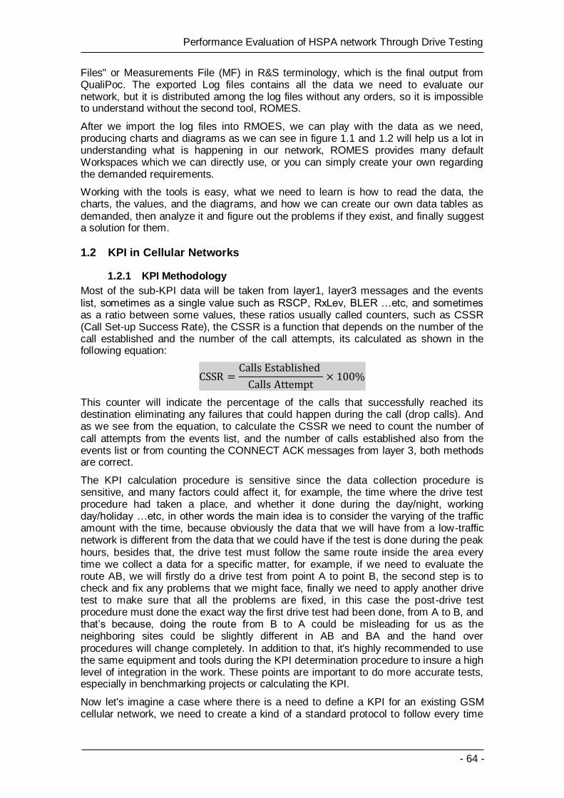
- 64 -


Files" or Measurements File (MF) in R&S terminology, which is the final output from QualiPoc. The exported Log files contains all the data we need to evaluate our network, but it is distributed among the log files without any orders, so it is impossible to understand without the second tool, ROMES.

After we import the log files into RMOES, we can play with the data as we need, producing charts and diagrams as we can see in figure 1.1 and 1.2 will help us a lot in understanding what is happening in our network, ROMES provides many default Workspaces which we can directly use, or you can simply create your own regarding the demanded requirements.

Working with the tools is easy, what we need to learn is how to read the data, the charts, the values, and the diagrams, and how we can create our own data tables as demanded, then analyze it and figure out the problems if they exist, and finally suggest a solution for them.

1.2 KPI in Cellular Networks

1.2.1 KPI Methodology

Most of the sub-KPI data will be taken from layer1, layer3 messages and the events list, sometimes as a single value such as RSCP, RxLev, BLER …etc, and sometimes as a ratio between some values, these ratios usually called counters, such as CSSR (Call Set-up Success Rate), the CSSR is a function that depends on the number of the call established and the number of the call attempts, its calculated as shown in the following equation:

This counter will indicate the percentage of the calls that successfully reached its destination eliminating any failures that could happen during the call (drop calls). And as we see from the equation, to calculate the CSSR we need to count the number of call attempts from the events list, and the number of calls established also from the events list or from counting the CONNECT ACK messages from layer 3, both methods are correct.

The KPI calculation procedure is sensitive since the data collection procedure is sensitive, and many factors could affect it, for example, the time where the drive test procedure had taken a place, and whether it done during the day/night, working day/holiday …etc, in other words the main idea is to consider the varying of the traffic amount with the time, because obviously the data that we will have from a low-traffic network is different from the data that we could have if the test is done during the peak hours, besides that, the drive test must follow the same route inside the area every time we collect a data for a specific matter, for example, if we need to evaluate the route AB, we will firstly do a drive test from point A to point B, the second step is to check and fix any problems that we might face, finally we need to apply another drive test to make sure that all the problems are fixed, in this case the post-drive test procedure must done the exact way the first drive test had been done, from A to B, and that’s because, doing the route from B to A could be misleading for us as the neighboring sites could be slightly different in AB and BA and the hand over procedures will change completely. In addition to that, it's highly recommended to use the same equipment and tools during the KPI determination procedure to insure a high level of integration in the work. These points are important to do more accurate tests, especially in benchmarking projects or calculating the KPI.

Now let's imagine a case where there is a need to define a KPI for an existing GSM cellular network, we need to create a kind of a standard protocol to follow every time

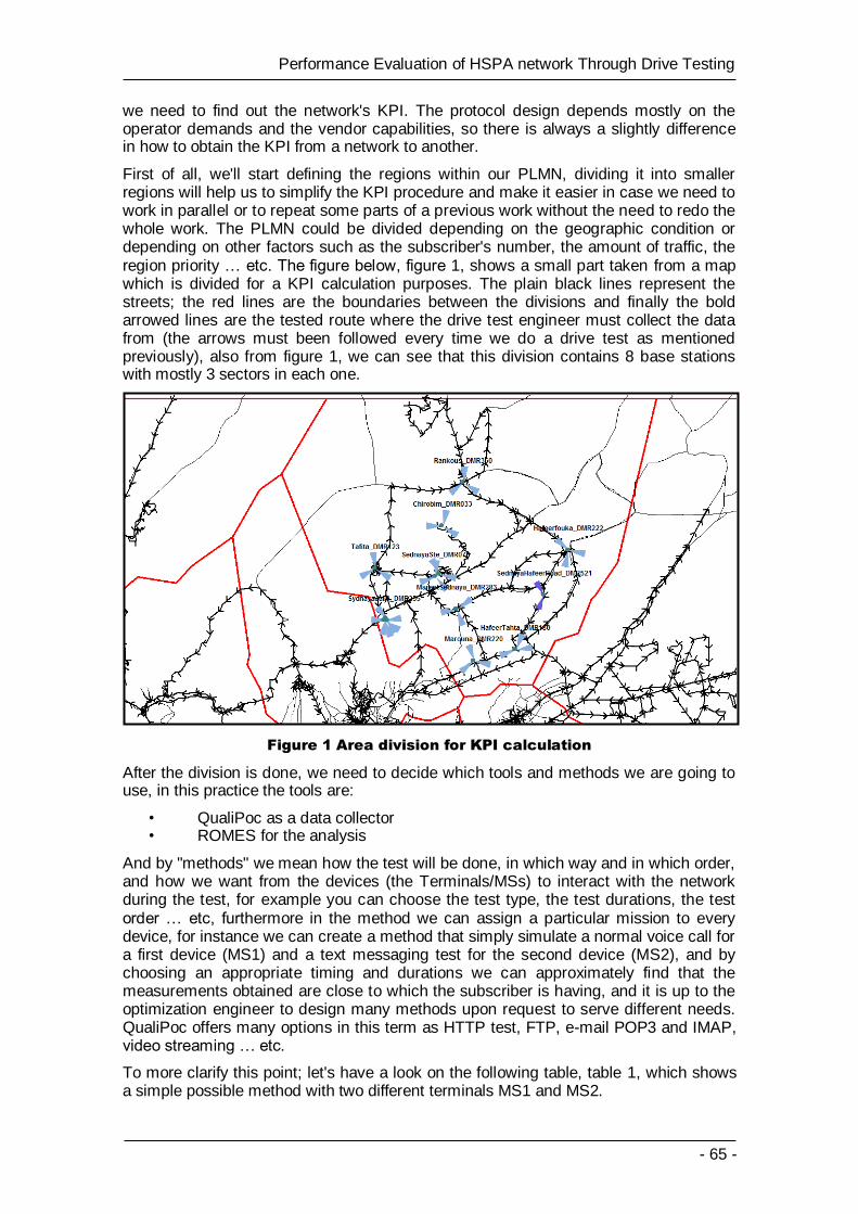
- 65 -


we need to find out the network's KPI. The protocol design depends mostly on the operator demands and the vendor capabilities, so there is always a slightly difference in how to obtain the KPI from a network to another.

First of all, we'll start defining the regions within our PLMN, dividing it into smaller regions will help us to simplify the KPI procedure and make it easier in case we need to work in parallel or to repeat some parts of a previous work without the need to redo the whole work. The PLMN could be divided depending on the geographic condition or depending on other factors such as the subscriber's number, the amount of traffic, the region priority … etc. The figure below, figure 1, shows a small part taken from a map which is divided for a KPI calculation purposes. The plain black lines represent the streets; the red lines are the boundaries between the divisions and finally the bold arrowed lines are the tested route where the drive test engineer must collect the data from (the arrows must been followed every time we do a drive test as mentioned previously), also from figure 1, we can see that this division contains 8 base stations with mostly 3 sectors in each one.

Figure 1 Area division for KPI calculation

After the division is done, we need to decide which tools and methods we are going to use, in this practice the tools are:

• QualiPoc as a data collector • ROMES for the analysis

And by "methods" we mean how the test will be done, in which way and in which order, and how we want from the devices (the Terminals/MSs) to interact with the network during the test, for example you can choose the test type, the test durations, the test order … etc, furthermore in the method we can assign a particular mission to every device, for instance we can create a method that simply simulate a normal voice call for a first device (MS1) and a text messaging test for the second device (MS2), and by choosing an appropriate timing and durations we can approximately find that the measurements obtained are close to which the subscriber is having, and it is up to the optimization engineer to design many methods upon request to serve different needs. QualiPoc offers many options in this term as HTTP test, FTP, e-mail POP3 and IMAP, video streaming … etc.

To more clarify this point; let's have a look on the following table, table 1, which shows a simple possible method with two different terminals MS1 and MS2.

- 66 -


MS Test Item Description

MS1 Coverage (RxLev) Idle mode

MS2 Quality (RxQual)

Dedicated Mode - Voice Calls - Destination Number: 166 - Originate Mode: GSM - Call Type: Continuous call - Setup Timeout(s): 45 - Exceptional Interval(s): 10 - Call Start Mode: Idle

Table 1 Possible method for DT

From the table above, we can see that the test will use two mobile phones during the test, the first one MS1, will be in the idle mode, that means it will be connected to the network but not active in terms of exchanging traffic, from MS1 we are going to obtain the average value of the network's coverage (also called RxLev or the received signal intensity level), also by keeping the MS in the idle mode we can check the cell selection and reselections procedures, while in the second terminal MS2 we can observe the hand over procedures between the terminal and the base stations, MS2 will be used to test the quality (RxQual) of the network when the traffic channels are used, so MS2 will be used in a dedicated mode, which means traffic exchanging from/to the terminal and the network. From the description of MS2 we can imagine very accurately how the test will be done, for example in this method we are using a voice test to check our network quality, and we are doing that by establishing a call with the fixed number: 166, this number is fixed just for testing purposes. Choosing a fixed number is important to maintain the stability of the tests, for instance, using another mobile phone as a destination number will lead to different results for sure. Besides that, from table 1, we can see that the originating mode is only GSM, and only GSM means that the cell phone will listen only to the GSM network and communicate with it. The call type is continuous, that means, in an ideal situation we need to make only one call when the test starts and hang up when the test is finished. Furthermore, inside the table we can see that there are two kinds of counters, the setup timeout counter, and the exceptional interval counter, the first one which counts 45 seconds will be triggered once we start the test along with the call establishing procedure, if the terminal failed to connect to the network within this 45 seconds an alarm will be activated. The second counter serves another meaning; this counter tells how much time we should wait until the MS can connect to the network again after a failing occurred (drop call). Finally notice that we used two terminals, MS1 and MS2 simultaneously, ROMES has the capability to connect up to 12 devices at the same time which certainly save us time and expenses. After we decided our regions, routes, tools and methods, we can start the drive test and begin the data collection procedure.

Once all the routes have been scanned as scheduled, and a number of "log files" are produced we can start organizing the data and analyze it. In this example case we'll assume that the required full KPI is consist of only 3 measurements, which are two values (RxLev, RxQual) and one counter CDR (call drop rate) so to obtain the full KPI for the studied region we need to find out and calculate RxLev, RxQual and CDR. Figure 2 shows the MS1 results after the test.

- 67 -


Figure 2 MS1 results after testing

The figure above shows the different values that we obtained for the RxLev via MS1; we can see how the values are distributed through the map and how easy it becomes to locate the weak spots in our region. Also we can represent the data in a histogram or a table, see figure 3

Figure 3 Representing data through Histograms

The number above each column stands for the statistical percentage density for each value, which means more than 72% of the samples are between -80dB ~ -10dB and about 10% of them are in the critical zone. Now do these kinds of RxLev values satisfy our needs? The answer for this question depends on the values requested by the operator, if the operator asked that more than 70% of the samples must be considered as good (-80dB~-10dB), then we can say that the RxLev value meets the first sub-KPI, if not, whether because the average RxLev is below 70% or because the KPI margin is higher than 70%, then we can say that the RxLev value didn't meet the defined KPI and we need to work on this issue in order to increase the RxLev value.

Now let's check the MS2 results in figure 4:

- 68 -


Figure 4 MS2 results after testing

Figure 4 shows the same voice quality which the subscriber is receiving, we can notice that almost all the bad spots in figure 2 (RxLev), are the same in figure 4, that is usually correct but not always, in some cases good receiving signal doesn't mean good quality as well, external interferences or a high level of fading could cause a situation where the signal intensity is high while the quality is bad.

Here also we can represent the data in different way, which gives us more options in order to understand and analyze the data, figure 5 is a histogram for the RxQual samples.

Figure 5 RxQual in histogram

The RxQual has 8 values [0~7], 0 is the best while 7 is the worst, and from figure 5 we can see that 13% of the samples are considered as bad quality, while about 80% considered as good, it is up to the operator to decide whether these percentages are good enough or not.

So now we already took a look on some sub-KPIs that we can obtain directly from the analyzer (RxLev and RxQual), now let's try to calculate the 3rd requirement sub-KPI, the CDR. The call drop rate can be defined as: it's a ratio of the abnormally disconnected calls to the total number of established calls during the test time, so the CDR will be calculated by counting the number of the call established and the number of dropped calls as the following equation.

- 69 -


Going back to the log files we can obtain the missing values in the equation, figure 6 shows how many dropped calls occurred and its distribution.

Figure 6 Dropped calls in the studied cluster

As we can see from figure 6, we got 10 dropped calls, which is the first variable in the equation, but we still have some issues when counting the call established number, as we can see from table 18 we used a method in which the test call is continuous, so in practical the number of the established calls are 1, plus the calls that have been established after every drop call, that will give us 10 more, and by applying these numbers to the equation we find that the CDR is about 90% which considered as a complete fail in any network, but, this value is misleading, its far away from being accurate and it doesn't give us an useful information about the network we are testing. To fix this we need to use another method to fulfill the requirements, for example in case we need an accurate CDR we can use the method shown in table 2.

MS Test Item Description MS1 Coverage (RxLev) Idle mode

MS2 Quality (RxQual)

Dedicated Mode - Voice Calls - Destination Number: 166 - Originate Mode: GSM - Call Type: discrete

- call duration: 50 - Setup Timeout(s): 45 - Exceptional Interval(s): 10 - Call Start Mode: Idle

Table 2 Test method for more accurate CDR

- 70 -


There are two more options in this method, now MS2 will do a number of discrete calls, which means more call established messages will appear and the CDR ratio will become more reasonable and useful. That means that we need to design the methods depending on what exactly we need, using multiple devices during the test makes this easier.

p.s. other way to solve this issue without changing the method used, is by doing an approximation for the CDR by obtaining the ratio between the number of the dropped calls and the overall test time duration, but this way is not accurate and it is not preferable by the operators or the optimization engineers.

As a conclusion, the key performance indicator is a measure to evaluate the performance of the network; and it always must follow a specific protocol to obtain it as a standard, and we should know how the test method, timing, or changing the routes could affect the KPI calculation.

The next part will introduce the most common KPIs in different cellular network technologies, GSM, UMTS and LTE.

1.2.2 KPI in different technologies

Each cellular technology has its own sub-KPIs, some of them are common like most of the counters, and some of them are determined for one technology, to simplify the sub-KPIs usage we can divide them into several categories:

Accessibility: The accessibility KPI counters measure the user ability to obtain the requested services from the network when needed. These kinds of counters usually observe the RRC connection and RAB setup.

Availability: Availability KPIs mainly indicates the availability of the network resources and gives a good idea about the traffic and the load.

Coverage: To monitor the coverage we need to monitor the interference between the cells and how the soft handovers are consuming the resources of the system. In a GSM system, the value RxLev (idle mode) is used as a coverage indicator.

Mobility: Mobility KPIs are mainly used to monitor the different types of handovers, and cell reselection.

Retainability: Retainability is defined as the ability of a user to stay connected to the requested service for the required duration once connected and till the service is no longer needed.

Traffic: Traffic KPIs are used to evaluate and observe the traffic regulation in the system; whether it was CS converted to Erlangs, or PS Traffic.

Integrity: mainly related to the block error rate.

These are the main categories for the cellular networks in general, in the following we will point out some of the most used KPIs in different technologies depending mostly on the 3GPP standardization.

In the following section we present some of the most used KPI in different technologies in a table form showing the name of the KPI its category and its formula. For more explanations regarding this topic please see Annex E for more details.

- 71 -


1.2.2.1 KPI in GSM

KPI Name Category Formula

CSSR Accessibility

CDR Retainability

CSR Accessibility

HOSR Mobility

LAUSR Mobility

CST Accessibility None

RxQual Coverage None

RxLev Coverage None

SQI Coverage None

TA Coverage None

Table 3 KPI in GSM

- 72 -


1.2.2.2 KPI in UMTS

KPI Name Category Formula

RABESR Accessibility

RRCCESR Accessibility

USAR Accessibility

GASRCS Accessibility

UPDPCASR Accessibility

USASR Accessibility

RARR Retainability

SHOSR Mobility

HHOSR Mobility

IRATHOSR-PS Mobility

RabEstabTotalPS Availability

CellAvailability Availability

Table 4 KPI in UMTS

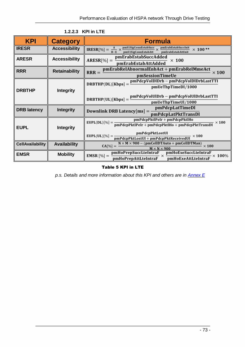
- 73 -


1.2.2.3 KPI in LTE

KPI Category Formula IRESR Accessibility [ ]

**

ARESR Accessibility [ ]

RRR Retainability

DRBTHP Integrity

[ ]

[ ]

DRB latency Integrity [ ]

EUPL Integrity

[ ]

[ ]

CellAvailability Availability [ ]

EMSR Mobility [ ]

Table 5 KPI in LTE

p.s. Details and more information about this KPI and others are in Annex E

- 74 -


1.3 Exercise 1: QualiPoc

This chapter will introduce a basic tutorial for using QualiPoc as a data collector tool. In the first part of this tutorial which aims to make the student familiar with the tool, we are going to do a simple voice test, then later students will do the same test but with some feature added, the last part is creating a data test (HTTP, FTP … etc). The Log Files/Measurement Files obtained in this exercise will be analyzed with the ROMES tool in another lab exercise.

Figure 7 QualiPoc Icon

1.3.1 Before Starting

Before launching the program from its icon as shown in figure 7, we need to make sure that the GPS and the Data Traffic options are enabled and working appropriately in the mobile device, and the Wi-Fi option is disabled. Also to ensure that the measurement tests run correctly, you need to disable the automatic date and time update feature on the device, for example, touch "Settings""Date & Time" "Automatic", and ensure that the automatic option is disabled.

1.3.2 Running QualiPoc

The main program interface is shown in figure 8, and we can find that it consists of multiple tabs, to preview the rest of them scroll the screen horizontally.

p.s. after updating the tool some snapshots might slightly differ.

- 75 -


Figure 8 QualiPoc main interface

From the tab "status" we can observe the status of the device, the tool, the GPS and the network in general, what we can check here before we start the test is whether we are using a forcing function or not, the GPS status which must turn from "connecting" to "valid position" after some seconds, if the status were "Invalid position" this means that the tool is not able to provide a geographical information for our test and in the most of the cases this will make the test not useful at all, because although the measurements occur in different time they will be placed in the same geographical point, Furthermore from the "Status" tab we can see the "last started test" and how many cycles that this test already finished, knowing that the number of cycles is adjusted before the test (Job in the QualiPoc terminology) started. The "Job success rate" which is an internal KPI that shows how the job/test has been handled within the tool, for example if the JSR was 50% that means that only 50% of the test is done successfully and the other 50% has been failed (for example 50% of the cycles are not done properly or not done at all), that could happen for many reason, for example the tool can't connect the network because a lack of coverage. Below the JSR we can find some pre-defined KPIs that QualiPoc offers, these KPIs are fixed by the manufacturer and test-dependent, for example the call setup time (CST) for a "call to any number" test and "Throughput" for an "HTTP transfer" test. Statistics represent the number of successfully completed tests as well as average, minimum, and maximum KPI results. Also, in the top of the screen we can find that the device is in the idle status listening to the network broadcasting and ready to establish a connection.

Scroll the screen horizontally and see the default tabs in QualiPoc, you can notice a set of "Technologies" tabs, such as GSM, GPRS, HSDPA, LTE … etc. These kinds of tabs provide the details of the available/used technology. The technology tabs change automatically depending on the technology the device is using, so if the device is connected to HSDPA network only the tabs related to this technology will appear, in

- 76 -


case the device made a handover to an LTE network the HSDPA tab will be replaced by the LTE tab.

Also you can notice some other tabs as the "Log" tab; this tab will be activated once the recording starts, otherwise it will be empty. This tab provide all the information related to the job/test execution in time such as (job started, start idle monitoring, Job stopped … etc) also it will provide you with information related to the device itself such as the statues of the device battery. See figure 9.

Figure 9 Log tab in QualiPoc

In the "Test" tab, you can see the summary of the on-going test and the corresponding KPI chart. The "Cells" tab provide information about the serving cell and the neighboring cells with its basic information, the information within this tab will vary with the technology in use. The "Coverage" tab is concerned in showing the coverage information for the corresponding technology in a chart form, for example RxLev in GSM and RSCP in UMTS. The tabs "Layer 3", "IP" and "Events" will show all the information that occurs between device and the network depending on the test you are using. The "Map" and the "Indoor" tabs are used to show the positioning information related to your test. The notification tab shows you if an alarm is activated, this tab will be discussed later with more details.

Now in your device, start QualiPoc and take a look on the main tabs, try to answer the following questions:

Exercise .1 who is the operator and what is the technology that the device is using?

Exercise .2 where you can find the information related to paging procedure between the network and the device?

Exercise .3 find the power indicator in the current technology that the device is using. In a UMTS network what is this indicator used for?

QualiPoc offers some quick help functions, when pressing the up-arrow button in the bottom of the screen in figure 8, a new tab list will appear as shown in figure 10, notice that this functions are available in all the tabs.

- 77 -


Figure 10 five properties for a quick help

1- Idle monitoring: to start recording the information in a log file while the device in the idle mode, in this case no need to create a test/job (the job option will be disabled), but note in case the device received or started a connection separately from QualiPoc all the signaling data will be recorded as well. If you are applying any job the recording will start automatically, notice that the QualiPoc icon in the top of the screen near the GPS icon will change from grey to red while recording, see figure 11.

Figure 11 QualiPoc icon while recording

2- Freezing: to freeze and unfreeze the monitors when needed, meanwhile the tool will keep recording, this option is useful for the user to check some parameters while testing, as the data changes rapidly in the screen.

3- Screen capture: to do a screenshots and save them directly to the SD card.

4- Photo marker: capture a photo with the device camera and save it in the SD card, if we are in the recording mode the photo will be attached to the log file.

5- Setting: the setting options for the current monitor/tab. For example by pressing this button while you are in the in the "Layer 3" tab you will be able to filter some messages from your screen to reduce the amount of data shown on the screens, notice that all the filtered messages will be recorded in the log file. If you press this button while you are in a technology tab such GSM you can

- 78 -


customize the GSM tab by adding, removing or rearranging the measurements in the tab in a way that suits the tester, also this is only to help you view the data on the screen, the log file will include all the measurements whither it is shown in the screen or not.

Also by touching the left button in the device, a new list will appear, see figure 12.

Figure 12 left button option

The first button "Jobs" leads you directly to the Job/test properties where you can choose the kind of test you want, or to start a previously saved Job.

The "Results" option displays the successfully recorded files in the device, while the "Settings" option will be discussed later.

The "Replay" option will be used to view previous recorded log files, when pressing this option a new screen will appear showing the QualiPoc library; from there you can choose the log file you need to replay. Notice that when you are in the replying mode the device will stop recording, and the QualiPoc icon will turn into blue, and you can see (null/null) near Replay instead of (Technology/operator) as in the recording mode, see figure 13. Also at the same figure we can see that the left button options which we discussed above are slightly different, now we have the "load file" option to load any of our previous work, and (Live) to switch from the Replaying mode to the recording standby mode.

- 79 -


Figure 13 the Replay mode

Furthermore, if you pressed the arrow button while you are in the replay mode, a set of playing options will appear as shown in figure 14.

Figure 14 Replaying options

The last button in figure 14 is used to choose a starting point for our replaying, for example if your test includes many cycles of calling/hanging up or a set of some sequential tasks you can choose at which cycle/task you want to start the replaying, which could save you some time in the field, in figure 15 a list of possible starting points is shown to choose from.

- 80 -


Figure 15 choosing a starting point for a replay

1.3.3 Preparing QualiPoc for tests

In this section we will prepare QualiPoc in general to be ready for any kind of test. As we saw in the introduction, QualiPoc offers many kind of different tests such as CALL tests, DATA tests MESSAGE tests, Idle monitoring and the ability to do a multi-data test or a multi-mix test (you can execute many jobs in a parallel or a sequential way; for example you can make the tool do a voice test then a data test after that.

First of all you need to be sure that the GPS and the maps are working in an appropriate way, the GPS data is essential as it gives the rest of the data a geographical meaning, without GPS the data will be placed in one position (one point) so interpreting the data will be impossible. Maps are important in the drive test phase and in the analyzing phase, they help us figuring out the problem and then fixing it, for example with maps it's easier to relate the traffic data to the demographical information, also by importing the CELL file which must be provided by the operator and contains all of the BTSs information such as positions, frequency, the cell general status …etc, this file must have a *.CSV format (usually) where each row corresponds to specific cell, for example the CELL file format for UMTS is (Name- Technology- UARFCN- PSC- Lon- Lat- MCC- MNC- TAC- CellId- Direction), by importing this file we can see in real time which cell is serving our connection and how is the hand-over procedure is being handled. To make sure that the GPS and the maps are ready to be used go to QualiPoc settings from the map tab then to the map settings as shown in figure 16.

- 81 -


Figure 16 map and GPS settings

Usually for map engines we use Google maps, also check near "Map Mode" to enable the satellite mode, the second two options "the online mode" and "Display Cached Areas" are disenabled in case we chose the Google map engine, from "GPS device" you can choose to use the internal GPS device or an external one with a Bluetooth connectivity with the device, note that in many cases the internal GPS could fail due to its weak sensitivity, it's usually better to use an external GPS with better performance, be always aware (before and while the test) that the GPS data is showing on the screen (in the map tab) while you are testing and recording, see figure 17, if not, stop the test and fix the problem by choosing another area to test or by changing the GPS settings.

Figure 17 GPS and Map data

After making sure that the GPS device and the map are working with no errors, go back to the "QualiPoc Settings" and press on the "BTS information" option. See figure

- 82 -


18. If you were provided with the BTS information (the CELL file) previously you can use it in the tool by pressing on the technology related to the file you had then import it to the tool, once you finish importing the file successfully the BTS distribution will be shown in the map. After that, the tool is ready to start a test/job.

Note that using a CELL file or not does not affect our work in the data collection/ drive test phase, in contrary with the GPS and the positioning data as they are very important in this phase; you can use the CELL file in the analyzing phase as it could be imported to ROMES or any other analyzing tool.

Figure 18 BTS information

1.3.4 Idle Monitoring

Start QualiPoc in a serviced spot and make sure that everything is working and ready as explained before, by default the QualiPoc will start the idle monitoring which you can notice by looking in the technology tabs but without recording. Use the "Idle monitoring" function explained before to start recording, see figure 10. Keep the recording function working for one minute.

Now switch the recording function off, and turn the tool into the "Replay" mode from "Settings" as shown in figure 13. When pressing on "Replay" a list of previous Log files will appear, choose the log file you made, you can find it under the folder which is named by the test date and test type, for example your log file name might be something like: 2014-12-2_Idle monitoring. Open the file and start the replaying, use the replaying functions shown in figure 14.

Exercise .4 Within the UMTS PLMN try to find the PDP context activation messages in

QualiPoc and the IP address assisted for the device, if the messages weren't there what is the possible reason?

p.s. the log file the student created will be used later in ROMES for more analyzing.

- 83 -


1.3.5 More features

1.3.6 Customizing

Customizing helps you to control your workspace (crate a new one or edit the existing workspace), and the monitors, you can add some charts to view them in the test real time and in the recording mode. To start customizing go to "Settings" "Customizing". See figure 19.

Figure 19 customizing- adding a new tab

Press on the plus sign as shown in the figure above to add a new tab, you also can remove or change the place of the tabs. If you are interested in creating your own workspace and control all the tabs and monitors, press on the left button while you in the "Customization" and choose "Save Workspace", two option will appear as shown in figure 20.

Figure 20 creating new workspace

You can choose to create a new workspace or save the changes on the last used workspace. Within your workspace you can decide how many tabs you want to use and what kind of information (parameters) you want to show. To create your own monitor press on the eye button shown in figure 19, and then on the plus button "Create", see figure 21.

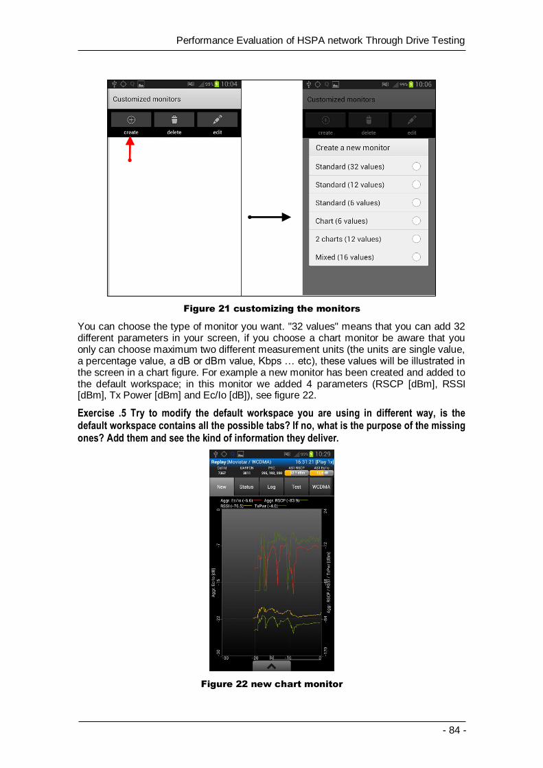
- 84 -


Figure 21 customizing the monitors

You can choose the type of monitor you want. "32 values" means that you can add 32 different parameters in your screen, if you choose a chart monitor be aware that you only can choose maximum two different measurement units (the units are single value, a percentage value, a dB or dBm value, Kbps … etc), these values will be illustrated in the screen in a chart figure. For example a new monitor has been created and added to the default workspace; in this monitor we added 4 parameters (RSCP [dBm], RSSI [dBm], Tx Power [dBm] and Ec/Io [dB]), see figure 22.

Exercise .5 Try to modify the default workspace you are using in different way, is the default workspace contains all the possible tabs? If no, what is the purpose of the missing ones? Add them and see the kind of information they deliver.

Figure 22 new chart monitor

- 85 -


1.3.6.1 Notifications

Notifications are another good feature offered by QualiPoc, by this feature you can set as many notifications as you want to inform you if an event or a particular value is occurred during the test. Notifications are useful but they are not necessary to complete the test, in other words they do not affect the result in the log files. The most used notifications are related to drop calls because such issues could affect the data of the test and sometimes could stop the job so the field engineer must be aware of this point. To set up a notification go to "QualiPoc Setting" and choose notifications, click in "Add notification" to create a new one. See figure 23.

Figure 23 creating a notification

From the event list choose what kind of event you need to keep an eye on, it will be either a layer 3 messages such the PDP context operations within the "Sessions Management", or a monitored parameter. For example try to set up a notification that informs you that the signal level is too low as this can cause some serious issues for the connection, for instance a low level signal in long time (seconds) can trigger the network to start a hand-over procedure for the current call even if the serving cell is working properly, in other words the cell is near and not loaded by the network traffic (in this case the signal might be suffering from some propagations issues). To create such notifications choose "Monitored Parameter" in figure 23, then choose a parameter to monitor, in our case we'll choose "RxLevSub[dBm]", see figure 24, as it is more accurate than the Full value because the full values are based upon the SACCH Multi-frame, whether they have been transmitted from the base station or not, and in case we are using DTX DL which is a mechanism used to stop the transmitter when the speech is paused the Full value won't be as accurate as the Sub values.

- 86 -


Figure 24 setting a monitored parameter

After selecting a parameter, select a condition (less/equal/not equal/greater), in this case choose "less" as a condition and put -100 (press the dot twice to print the minus symbol) in the argument box, this means that if the signal dropped below -100 dBm a notification will be activated. Also you can choose the alerting sound and whether you want a vibration alerting or not. By pressing "OK" you can see that the notification had appeared in the "Notifications Settings", you can enable or disable any notifications you have on the list, and when an alarm is activated because a notification had accorded the device will make a sound and another purple QualiPoc Icon will appear in the top of the screen, see figure 25. Notice that the activated notification will be applied in all the jobs.

Finally to view the notification history press on the notifications tab, and then press on the notification you interest in.

- 87 -


Figure 25 Notifications settings

If a notification had been occurred we can find it in the "Notifications" tabs, see figure 26.

Figure 26 notification detected

By clicking in the notification we can view the event history of the notification, see figure 27.

Exercise .6 Create other notifications for the following cases: A) The device is using HSPA network. B) The device is using LTE network. C) The GPS status is not valid. D) The Job success rate is less than 90%.

- 88 -


Figure 27 Notification history

1.3.6.2 Forcing Function

Another vital feature in all the recent drive test tools is the forcing function, by the mean of this feature we can control the technology we want to use via our device or the band (note that the available bands to control depends on the capabilities of the device itself), also we can prevent the device from doing any hand-over between the cells, or to force it to do a hand-over for a specific cell. Forcing function is easy to configure, but yet you can use it in many cases to determine and observe other parameters, for example you can create a Time Advance (TA) map for a specific cell by forcing the device to connect to this cell all the time, this will be useful as the TA parameter can be used as a HO trigger in the GSM networks.

You can use the force function in your entire tests/jobs by configuring this function from the "QualiPoc Settings", or you can use it only in a specific job by modifying the properties of this job. For instance, try to modify the previous job you created to add a forcing function to the test, first go to the job settings, press the left button "Load Job", find your job that you created press on "Advanced Job Settings" forcing. See figure 28. Note: In case you don’t want to change the original job you created early, from the "Job settings" left button "Duplicate jobs"choose the job you want to duplicate choose a new name then edit its properties as you need.

- 89 -


Figure 28 forcing function

After setting up the forcing function and starting a job, in the "status" we can notice that the forcing function is activated, see figure 29.

Figure 29 forcing function activated

Exercise .7 Apply a forcing function for your job by forcing the device to connect to a good signal level UARFCN, how many possible UARFCN there to choose among them?

- 90 -


1.3.7 Single voice call test

Voice call tests are easy to set up. In this test the QualiPoc device (device A) will establish a voice call through the provided network and technology by dialing the number of the destination device (device B), after the Device B answers, a countdown counter (the call duration) will start, after finishing the counter the call will be ended and (device A) will wait for some time (Pause timings) then start again, this procedure will be repeated as required (# of cycle).

1.3.7.1 Job creation

Go to any tab and press the left button, choose the option "Jobs", the last used Job will appear on the screen, to create a new job press on "Advanced Job setting", then the left button again and choose "Create new job", a list with four main options to choose among them will come into view, choose the first option "Single CALL tests". After choosing this option check near "Call to any Number", a new setting list specifically for call tests will appear. See figure 30 and figure 31.

Figure 30 single call test settings

- 91 -


Figure 31 Call to any Number Settings

Give the test a name, see figure 32, and set its properties (the timing and the destination phone number) so you can save and use it later when needed.

Figure 32 Job naming

After that press on "Timings and scheduling", change the parameters as the test requires. See figure 33.

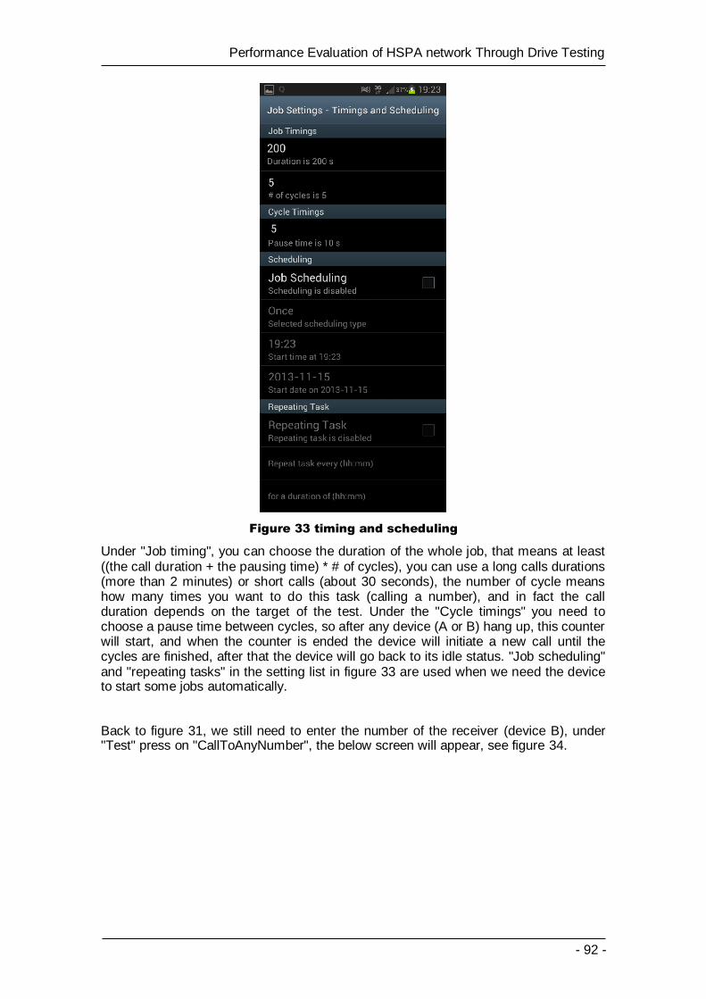
- 92 -


Figure 33 timing and scheduling

Under "Job timing", you can choose the duration of the whole job, that means at least ((the call duration + the pausing time) * # of cycles), you can use a long calls durations (more than 2 minutes) or short calls (about 30 seconds), the number of cycle means how many times you want to do this task (calling a number), and in fact the call duration depends on the target of the test. Under the "Cycle timings" you need to choose a pause time between cycles, so after any device (A or B) hang up, this counter will start, and when the counter is ended the device will initiate a new call until the cycles are finished, after that the device will go back to its idle status. "Job scheduling" and "repeating tasks" in the setting list in figure 33 are used when we need the device to start some jobs automatically.

Back to figure 31, we still need to enter the number of the receiver (device B), under "Test" press on "CallToAnyNumber", the below screen will appear, see figure 34.

- 93 -


Figure 34 continue job settings

The choosing of the destination number depends on our test targets, for example choosing a number for a fixed line will reduce the call establishment time as there no paging procedure involved, the delay caused by the paging procedure in GSM could be as long as 2.5s depending on some factors such as paging channel load, transmission delay of core network to BTS, paging repetition timer … etc. Moreover you will need to set a "max. call setup time", which means that if the call had not established within this time, the cycle will be ended and the tool will wait for 10 seconds (pause time) and try again. The "Call duration" must also be chosen properly, As has been said before, choosing the call duration is important and rely on what kind of data we want, for example choosing a long test call can help us having better statistics for the hand-over procedures between cells, while short and highly multiplied calls can give better statistics related to network connectivity; establishing and releasing sessions.

To save your work, from the "job setting", press the left button and choose "Save job". After you finish, go back to the basic screen by pressing the back button twice in the device. Finally Press the green button "start job". See figure 35.

- 94 -


Figure 35 Start Job

1.3.7.2 Job execution and results

After the job is started you can browse the tabs and observe the measurements. In figure 36 (snapshot from the replay mode for the previous job) you can see the "status" tab after the job is finished, also note that the technology tabs will appear automatically depending on the serving cell technology, you can browse the rest of the tabs for more details.

- 95 -


Figure 36 status tab after a test

Press the green loading bar as shown in the figure 36 above, a new list will appear showing that the job had succeed completely, under that you can see the CST for this GSM network is about 10 second which seems to be a little bit high.

The job will end automatically after the cycles are finished, you can also end it by pressing the left button in the device and then press "stop job", as in figure 37. QualiPoc will start recording once you press the "start job" button, and will end when the job is ended automatically or manually as mentioned before.

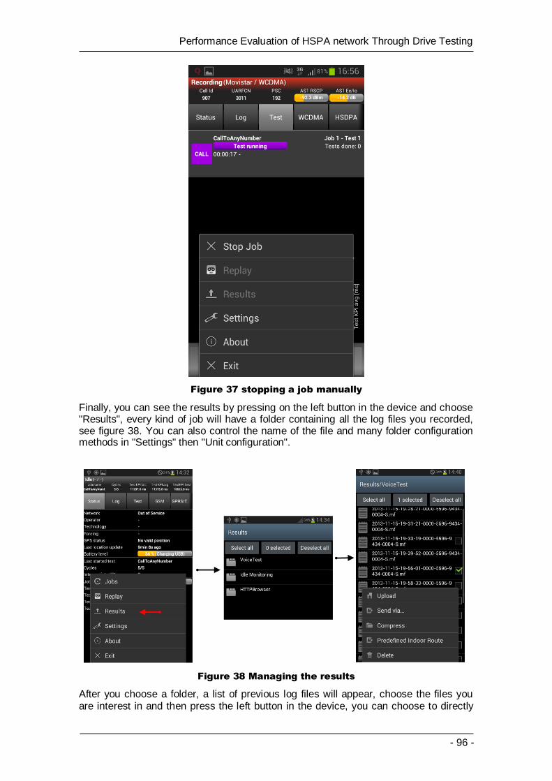
- 96 -


Figure 37 stopping a job manually

Finally, you can see the results by pressing on the left button in the device and choose "Results", every kind of job will have a folder containing all the log files you recorded, see figure 38. You can also control the name of the file and many folder configuration methods in "Settings" then "Unit configuration".

Figure 38 Managing the results

After you choose a folder, a list of previous log files will appear, choose the files you are interest in and then press the left button in the device, you can choose to directly

- 97 -


upload the result to a specific server (you need to set up the configuration first), or you can send it via Bluetooth or Gmail, also you can compress the files in order to save some space in your mobile SD card.

From figure 38 you can see that the measurement files have a long name (the test date, the test starting time and the device serial number), in later versions of QualiPoc you can modify how you want to name your log files. If you just need to modify the folders name in order to better organize your data go to "Settings""unit conversion" under the "Result Folder" check or uncheck the properties as you need, see figure 39. It's recommended to follow the same way of naming the folders as show in figure 39 as the "System" (the system is QualiPoc) and the "Device" are always common in our case. (In the newest versions of QualiPoc there is more option to control the naming of the log files).

You can also scroll up and down while you are in the "unit conversion" screen, as you can see you can enable or disable many properties such as "Auto Compression" (compressing the log files in order to send them later), or whether you prefer to upload the log files manually or automatically by adding the server information (the host URL, the connection type, the user name and the password for the server account … etc)

Figure 39 Modifying the folder naming

- 98 -


1.3.8 Forced voice call test

In the previous test you might noticed that that the technology tabs are changing which means that this job has been accomplished by more than one technology, the resulted log file will contain all the data about these technologies and how they interact together in the same PLMN, the previous test shows us in fine way the kind of QoS that the users are enjoying, but in case we are interested in one technology, or in case we encountered some problems in the interaction between one technology and another we need to separate the problem in order to better analyze it, so we need to use the forcing function mentioned before.


First we need to create another job the same way we created the previous one, but we need to force it to the technology we are interested on, from "Job Settings" "Advanced Job Settings" forcing function, then choose the kind of forcing you need, see figure 28. Also create some notifications that alarm u in case the test encounters some poor coverage areas, poor quality or a drop call. Note that you can change the type of the data you want to observe (even if some parameters are not shown in the screen they will be recorded in the log file and you can analyze them later using QualiPoc or ROMES), to manage the parameters shown under the technology tabs, first go to the technology tab and press the arrow button in the bottom of the screen then press the last button in the right as shown in figure 10, a new list will appear containing all the parameters related to the corresponding technology, you can add, remove or rearrange the parameters as you need. See figure 40.

Figure 40 customizing the observed parameters

Press on the symbol left to the parameter name (the red arrow) to move this parameter up or down, if you keep pressing on the plus sign at the parameter rights, a deleting option will appear, if you want to add more parameters press the sign button at the top of the screen, a new list will appear (shown also in figure 40), choose the parameter

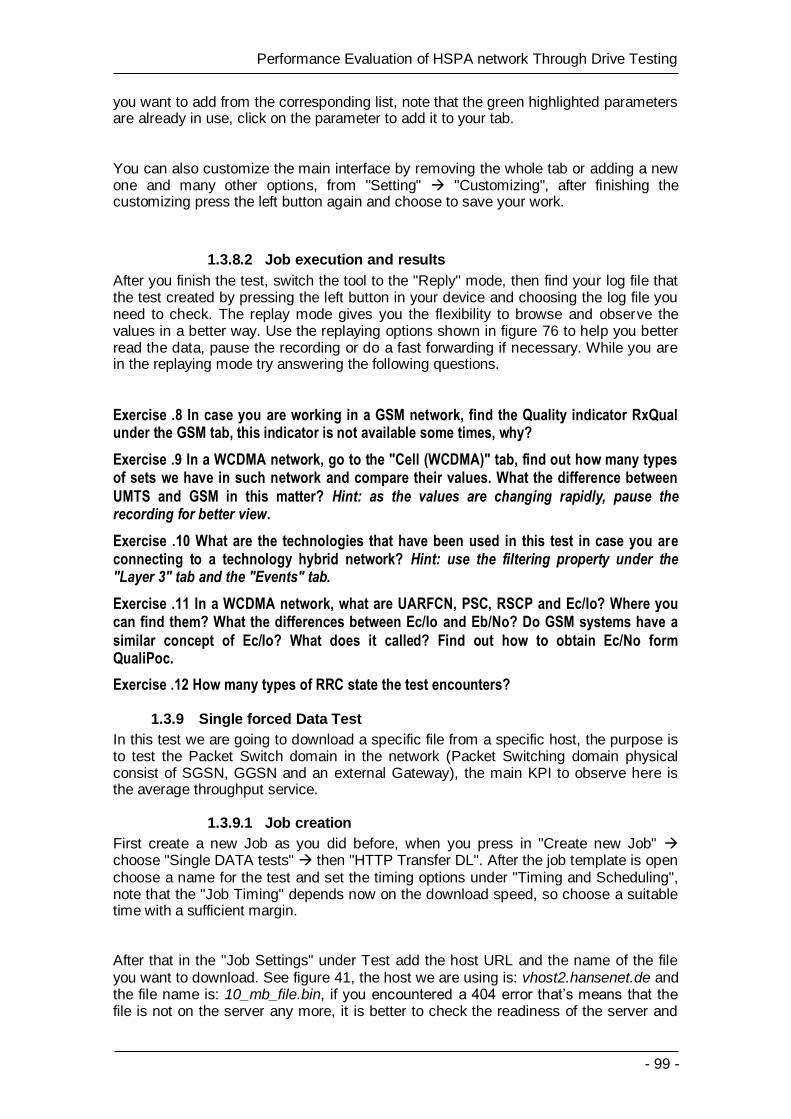
- 99 -


you want to add from the corresponding list, note that the green highlighted parameters are already in use, click on the parameter to add it to your tab.

You can also customize the main interface by removing the whole tab or adding a new one and many other options, from "Setting" "Customizing", after finishing the customizing press the left button again and choose to save your work.


After you finish the test, switch the tool to the "Reply" mode, then find your log file that the test created by pressing the left button in your device and choosing the log file you need to check. The replay mode gives you the flexibility to browse and observe the values in a better way. Use the replaying options shown in figure 76 to help you better read the data, pause the recording or do a fast forwarding if necessary. While you are in the replaying mode try answering the following questions.

Exercise .8 In case you are working in a GSM network, find the Quality indicator RxQual under the GSM tab, this indicator is not available some times, why?

Exercise .9 In a WCDMA network, go to the "Cell (WCDMA)" tab, find out how many types of sets we have in such network and compare their values. What the difference between

UMTS and GSM in this matter? Hint: as the values are changing rapidly, pause the recording for better view.

Exercise .10 What are the technologies that have been used in this test in case you are connecting to a technology hybrid network? Hint: use the filtering property under the "Layer 3" tab and the "Events" tab.

Exercise .11 In a WCDMA network, what are UARFCN, PSC, RSCP and Ec/Io? Where you can find them? What the differences between Ec/Io and Eb/No? Do GSM systems have a

similar concept of Ec/Io? What does it called? Find out how to obtain Ec/No form QualiPoc.

Exercise .12 How many types of RRC state the test encounters?

1.3.9 Single forced Data Test

In this test we are going to download a specific file from a specific host, the purpose is to test the Packet Switch domain in the network (Packet Switching domain physical consist of SGSN, GGSN and an external Gateway), the main KPI to observe here is the average throughput service.


First create a new Job as you did before, when you press in "Create new Job" choose "Single DATA tests" then "HTTP Transfer DL". After the job template is open choose a name for the test and set the timing options under "Timing and Scheduling", note that the "Job Timing" depends now on the download speed, so choose a suitable time with a sufficient margin.

After that in the "Job Settings" under Test add the host URL and the name of the file you want to download. See figure 41, the host we are using is: vhost2.hansenet.de and the file name is: 10_mb_file.bin, if you encountered a 404 error that’s means that the file is not on the server any more, it is better to check the readiness of the server and

- 100 -


the file from the internet browser before starting the test. Keep the user name and the password empty as this sever doesn't need any authentication to download from. In "Selected max test duration" put a reasonable number to finish each test, notice that the job time is the time for all the test cycles to finish, while the test duration is the duration for each test alone.

Figure 41 single data test configuration

In this test the size of the file we are downloading is 10MB, in the 3G technology this file is considered small, in other words there is high chance that you won't reach the maximum throughput when you do this test. If testing the throughput is major for some cases choose a larger file. When you finish set the forcing function for this job to UMTS as we will focus on HSPA and LTE later.

After you finish creating and saving the job, go the job main screen and press "Start" as shown in figure 42.

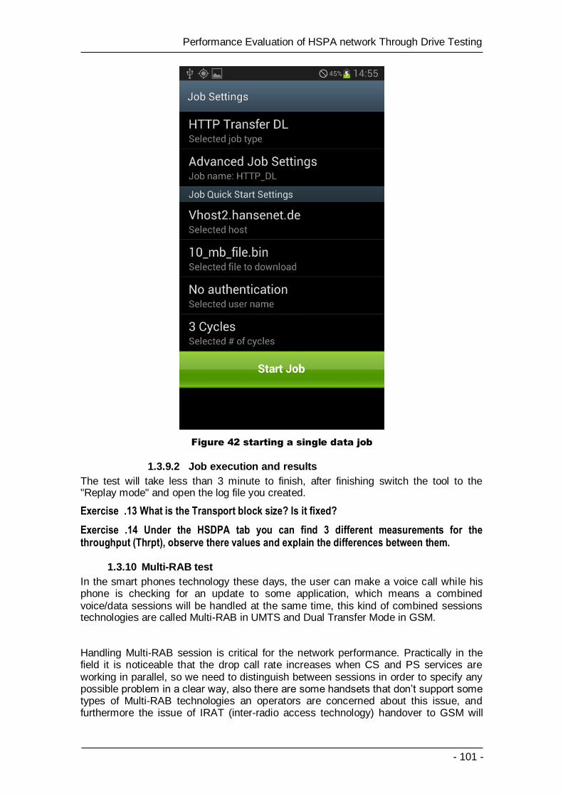
- 101 -


Figure 42 starting a single data job


The test will take less than 3 minute to finish, after finishing switch the tool to the "Replay mode" and open the log file you created.

Exercise .13 What is the Transport block size? Is it fixed?

Exercise .14 Under the HSDPA tab you can find 3 different measurements for the throughput (Thrpt), observe there values and explain the differences between them.

1.3.10 Multi-RAB test

In the smart phones technology these days, the user can make a voice call while his phone is checking for an update to some application, which means a combined voice/data sessions will be handled at the same time, this kind of combined sessions technologies are called Multi-RAB in UMTS and Dual Transfer Mode in GSM.

Handling Multi-RAB session is critical for the network performance. Practically in the field it is noticeable that the drop call rate increases when CS and PS services are working in parallel, so we need to distinguish between sessions in order to specify any possible problem in a clear way, also there are some handsets that don’t support some types of Multi-RAB technologies an operators are concerned about this issue, and furthermore the issue of IRAT (inter-radio access technology) handover to GSM will

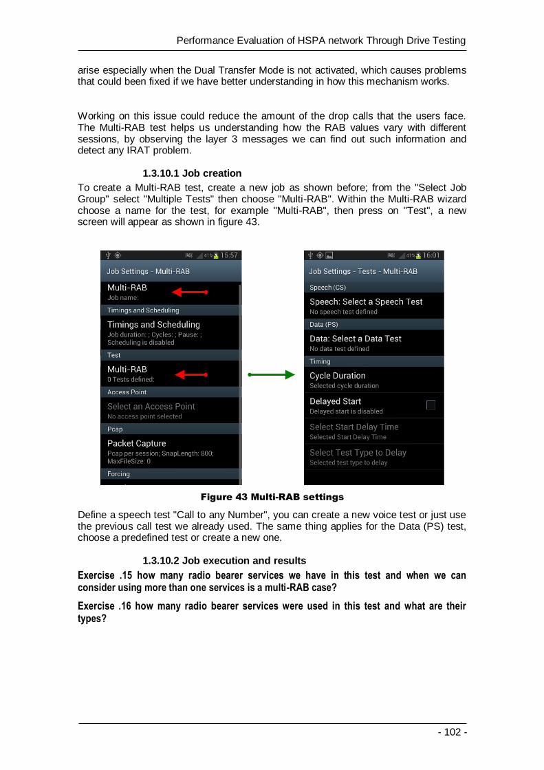
- 102 -


arise especially when the Dual Transfer Mode is not activated, which causes problems that could been fixed if we have better understanding in how this mechanism works.

Working on this issue could reduce the amount of the drop calls that the users face. The Multi-RAB test helps us understanding how the RAB values vary with different sessions, by observing the layer 3 messages we can find out such information and detect any IRAT problem.


To create a Multi-RAB test, create a new job as shown before; from the "Select Job Group" select "Multiple Tests" then choose "Multi-RAB". Within the Multi-RAB wizard choose a name for the test, for example "Multi-RAB", then press on "Test", a new screen will appear as shown in figure 43.

Figure 43 Multi-RAB settings

Define a speech test "Call to any Number", you can create a new voice test or just use the previous call test we already used. The same thing applies for the Data (PS) test, choose a predefined test or create a new one.


Exercise .15 how many radio bearer services we have in this test and when we can consider using more than one services is a multi-RAB case?

Exercise .16 how many radio bearer services were used in this test and what are their types?

- 103 -


ANNEX B: QualiPoc Tutorial

Answers


- 104 -


Table of Content

1. ANNEX B: QualiPoc Tutorial answers ............................ - 105 -

1.1 “Before Starting” Section answers ........................................................... - 105 -

1.2 Idle Monitoring test answers .................................................................... - 105 -

1.3 Forced voice call test answers ................................................................. - 106 -

1.4 Single forced Data Test answers ............................................................. - 110 -

1.5 Multi-RAB test answers ........................................................................... - 110 -

- 105 -


1. ANNEX B: QUALIPOC TUTORIAL ANSWERS

1.1 “Before Starting” Section answers

Exercise .1 This information is available in the up of the QualiPoc screen (in case there is no coverage this information will not be available).

Exercise .2 From the "Layer 3" tab we can find all the paging requests messages and the RRC messages.

Exercise .3 the power indicator will vary with the technology for example it is Tx power for the GSM technology, and for UMTS networks you can find the power indicator under the WCDMA tab named TxPwr. In umts this indicator can be found in the layer 1 messages, mainly there is 3 kind of power control in a umts system, the "outer loop power control" adjust the the UE transmitted power to meet the required SIR and to overcome the near-far effect, this helps a lot in saving the battery of the device. This parameter usually have an inverse relationship with RSCP and the quality indicators of the network.

1.2 Idle Monitoring test answers

Exercise .4 A PDP context procedure will activate once the device is connected to the data packet domain, and as a result for this procedure the device will be supported by an IP adderss. The PDP messages are shown on the "Layer 3" tab, and by clicking on the messages we can find all the details which we want such the IP address. More likely the student will not find these messages in the layer3 tab if the data traffic is enabeld before because in this case the PDP messages has been recived but not shown in the screen (the data traffic mode is enabeled once the mobile is turned on as a defualt), so to see the PDP messages turn the mobile traffic mode off while you in the QualiPOc interface, then turn it on, you will notice that a PDP procedure is initiated. See figure 36.

Exercise .5 There is only one missing tab in the default workspace, this tab called "RC Log", this tab shows all the information related to the "Remote controlling" operation mode. If the tool is on the "Handheld" mode this tab will disappear even if it was chosen before. You can control the operation mode from "Settings" "Unit Configuration" under the Operation modes choose the type of mode you want. figure 44 shows the function of all the remaining tabs.

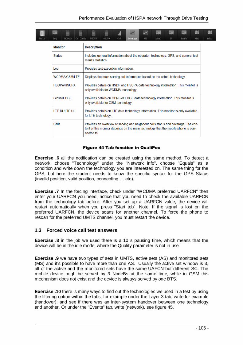
- 106 -


Figure 44 Tab function in QualiPoc

Exercise .6 all the notification can be created using the same method. To detect a network, choose "Technology" under the "Network info", choose "Equals" as a condition and write down the technology you are interested on. The same thing for the GPS, but here the student needs to know the specific syntax for the GPS Status (invalid position, valid position, connecting … etc).

Exercise .7 In the forcing interface, check under "WCDMA preferred UARFCN" then enter your UARFCN you need, notice that you need to check the available UARFCN from the technology tab before. After you set up a UARFCN value, the device will restart automatically when you press "Start job". Note: If the signal is lost on the preferred UARFCN, the device scans for another channel. To force the phone to rescan for the preferred UMTS channel, you must restart the device.

1.3 Forced voice call test answers

Exercise .8 in the job we used there is a 10 s pausing time, which means that the device will be in the idle mode, where the Quality parameter is not in use.

Exercise .9 we have two types of sets in UMTS, active sets (AS) and monitored sets (MS) and it's possible to have more than one AS. Usually the active set window is 3, all of the active and the monitored sets have the same UAFCN but different SC. The mobile device migh be served by 3 NodeBs at the same time, while in GSM this mechanism does not exist and the device is always served by one BTS.

Exercise .10 there is many ways to find out the technologies we used in a test by using the filtering option within the tabs, for example under the Layer 3 tab, write for example (handover), and see if there was an inter-system handover between one technology and another. Or under the "Events" tab, write (network), see figure 45.

- 107 -


Figure 45 filtering the Events

Make sure that the "Disable" option is active by the appearing of blue bar under in the disable button. Also make sure that you already scanned the whole record. We can see that in this specific case we used 2 technologies, EDGE and GPRS.

Exercise .11 RSCP: Received Signal Code Power, the power received by the receiver, it indicates the signal strength, similar to RxLev in GSM. PSC: the Primary Scrambling Code, in a UMTS system each cell has one PSC, so this value separates cells. UARFCN: UTRA Absolute Radio Frequency Channel Number, it used to identify the frequency in a UMTS band, the URFCN value related to the corresponding frequency, which means you can find out the frequency you are using by knowing the numerical relation between the UARFCN and the frequency. Ec/Io: the ratio of the energy per chip in CPICH to the total received power, it is similar to C/I in GSM systems, while Eb/No is the bit energy over the noise level, in UMTS systems Io = the cell interference + the surrounding cells interference + the noise level, Ec/Io is an indicator for the signal quality.

Eb/No=processing gain + SIR, this metric depends on the service, for example the required Eb/No for the CS is higher than the PS because in CS is more real time so it have less flexibility of using the error correction mechanisms than PS.

You can obtain all these value using QualiPoc by observing the WCDMA tab, if the parameter doesn't exist, try to customize the tab and add the parameter you need by clicking on the last button in the quick help function (the arrow in the bottom), see picture 10 in the tutorial. (It is explained in the tutorial as well).

In QualiPoc you can’t find the Eb/No value directly, to find this value firstly you need to know what kind of service we are using (CS-12.2, PS-64, PS-128, HSDPA … etc), each service have a specific processing gain for example the PG for PS-64 is 18 dB, after that you can apply the equation above to find out the Eb/No.

- 108 -


Exercise .12 to find out the RRC states, go the technology tab in the recording mode, and click on the RRC state, a list will appear in the screen. Again make sure that the record is fully scanned, See figure 46.

Figure 46 RRC states

- 109 -


Figure 47 Throughput KPI

Figure 48 PDP messages

- 110 -


1.4 Single forced Data Test answers

Exercise .13 The transport size varies with the time, see figure 49. We can find the TB size by looking at the HSDPA tab. The TB conssist mainly of two parts, a fixed part and a dynamic one, the fixed part includes the CRC, TTI ... etc while the dynamic part can be changed every TTI to adapt the transmission rate to the rate instructed to MAC. (in the idle mode the TB value will be empty.

Figure 49 TB size

Exercise .14 By default customization we can observe 3 types of throughputs, the HS-DSCH Throughput: this channel has been added in release 5, this channel caries the user data in the DL between the physical layer and the MAC and its rate will vary with the modulation used. Scheduled throughput: is the data throughput that the network uses according to the requests (CQI messages) from the mobile. Requested throughput: is the data throughput that the mobile requests according to the measured channel quality

1.5 Multi-RAB test answers

Exercise .15 The data RAB services are divided into 4 traffic classes: conversational class (real time traffic, high QoS required), Streaming class (lower QoS, unidirectional), Interactive class (is used to carry traditional internet services such as browsing) and background class (is used to transmit or receive data in background mode such as FTP, HTTP, SMS… etc.). And to consider a case a multi-RAB case we must be using two or more different classes.

Exercise .16 we have two different services (traffic classes): conversational (voice call) and background (HTTP download).

- 111 -


ANNEX C: ROMES R&S

Tutorial


- 112 -


Table of Content

1. ANNEX C: ROMES R&S Tutorial ..................................... - 113 -

1.1 Introduction about ROMES R&S .............................................................. - 113 -

1.2 Getting started with ROMES R&S............................................................ - 113 -

1.2.1 Starting R&S ROMES ................................................................... - 113 -

1.2.2 ROMES R&S Workspace: ............................................................. - 116 -

1.2.3 Opening a measurement file: ........................................................ - 117 -

1.2.4 Analyzing the data and observing the view areas: .......................... - 119 -

1.3 Practical Exercises: ................................................................................ - 133 -

1.3.1 Analysis of Idle Monitoring Tests ................................................... - 133 -

1.3.2 Analysis of Voice tests .................................................................. - 134 -

1.3.3 Analysis of HSDPA Data tests ....................................................... - 134 -

1.3.4 Analysis of Multiple-tests (Multi-RAB test) ...................................... - 135 -

- 113 -


1. ANNEX C: ROMES R&S TUTORIAL

1.1 Introduction about ROMES R&S

ROMES is a drive test tool offered by Rohde and Schwarz, and like all the other drive test tools, ROMES allow us to make measurements of coverage, capacity and QoS of a mobile radio network and also to assess the performance of the network. ROMES offers a set of features in Speech Quality tests, combined indoor/outdoor tests and integrated algorithms for detecting and analyzing the network problems. It supports all the cellular technologies with the ability to do parallel measurements up to 12 mobile phones, which means 12 different tests at the same time (benchmarking tests will become easier and efficient).

1.2 Getting started with ROMES R&S

For the analysis of the data we took using the QualiPoc android phone we need to use the R&S ROMES (replay). We can observe all the information about the problems of the mobile network and create results reports and analyze the data in order to find the appropriate solution for network problems.

1.2.1 Starting R&S ROMES

When you start ROMES, a Startup wizard appears to allow you to choose how the ROMES will start, it gives you choices if you want to load a predefined workspace or project or if you want to start with an empty workspace. And also with the ability to load a measurement file when the program starts. The figure below shows you the startup wizard mentioned:

Figure 1 Startup Wizard

User: this option allows you to add or load users; each user has its own copy of the ROMES registry entry. Using different users will allow us to personalize ROMES for example with different vehicle ID, User ID …etc.

Mode:

- 114 -


Load project: allows you to open a project file already created before, and it opens a specific modules and views. A project file (*.rsproj) stores all information about the necessary modules and views for a certain measurement or evaluation task to improve the performance of R&S ROMES and the clarity of its GUI. However the project can only be created in the “measurement mode” which is not available in this lab.

Load workspace: allows you to load a predefined workspace when the ROMES starts. The workspace will be explained later in the R&S ROMES Workspace section.

Start with empty view areas: opens ROMES without any predefined workspace.

Measurement file:

Load measurement file: allows opening a measurement file immediately when ROMES starts.

User level:

Change user level:

- Normal: opens the minimum set of views required for the most analysis tasks.

- Advanced: opens additional views for more specific tasks.

- Expert: opens the full set of views.

User level definition files: allows you to load a custom user level created by the user. The figure 2 below shows you the user level window:

Figure 2 User Level

Since the “Normal” user level offers the minimums set of view, thus it’s suitable to be used for measurement for a fast performance. And the “Advanced” or “Expert” levels should only be used for investigation since they offer more options and can slow down the performance of the PC. So for this lab you can choose the “expert” level to get the full set of views in order to be familiar with them.

1.2.1.1 Welcome bar

When the ROMES starts, a welcome bar can be found on left side of the main window as shown in the figure 3 below. The welcome bar guides the user and gives him easy access to the most important functions in the ROMES R&S.

- 115 -


Figure 3 Welcome Bar

In the “replay only” mode we have two panels in the welcome bar, the first one is the analyze panel and the second one is the export panel.

Analyze panel: It gives you access to the latest measurement file opened for analyzing and also gives you access to the transmitter databases so you can load the BTS information in order to do the analysis process.

Export panel: it gives you access to the available export modules. For example you can export the map graphical information as an ASCII file to be analyzed using the “MapInfo” software, and that can be done by the “MIF export” option. Another example is the “KML/KMZ Export” that Exports measured signal data to Google Earth's Keyhole Markup Language format, either as compressed (kmz) or normal (un-compressed) files (kml). The exported data can then be easily visualized and analyzed according to the position it was measured at, using the Google Earth software package.

In addition, the welcome bar gives you a list of the shortcuts for all the functions in the ROMES R&S which can ease the use of the software. See figure 4.

- 116 -


Figure 4 Analyze and Export Panels

1.2.2 ROMES R&S Workspace:

Before start working, first you need to create a workspace. A workspace contains the device driver and the screen settings for the ROMES Session, which means that it contains all the parameters for the view windows like the size, type, position of the views, and the parameter types in each view but without any data because the data is not part of the workspace but can be found in the drive test measurement files created by the QualiPoc android phone.

You can create new standard workspace, save a user-defined workspace or load a previously created workspace from the “file” menu in the task bar shown in the figure 5 below.

- 117 -


Figure 5 Workspace

Try to open a workspace and get familiar with the process. Note that also when you open a measurement file, the software automatically opens a workspace and asks you to save it. In the next section you will find information on how to open a measurement file.

1.2.3 Opening a measurement file:

This section explains how to open a measurement file with ROMES in order to continue with the tutorial and later do the practical exercises.

Before opening a measurement file, you must convert the measurement file created by the QualiPoc android phone which has the extension (.mf) to the extension (.RSCMD) supported by ROMES R&S. and you can do that easily by using the additional installed software made by Rohde & Schwarz, called “QualiPoc Converter” as shown in the figure 6 below:

- 118 -


Figure 6 QualiPoc Converter

You can add the measurement files that you want to convert by the add button and then start conversion. After the conversion is done, the measurement files are ready to be opened by ROMES for analyzing. You can open the measurement files from the “file” menu shown in a previous figure (figure 5) or by using the analyze panel in the welcome bar for a quicker access. Once a measurement file is opened, a replay panel is opened in the welcome bar automatically. See figure 7.

Figure 7 Replay Control Panel

- 119 -


Replay Controls:

It shows you the replay control icons of the “replay bar”.

Figure 8 Replay Controls

Replay jump shows you additional features that can help in better controlling the replaying of measurement file.

Figure 9 Replay Options

The block mode: if the file contains several blocks, it shows you the list of blocks in the measurement file and allows you to jump to from block to block. However the capability of dividing the measurement file into several blocks is not supported by QualiPoc software.

The bookmark mode: if the file contains several bookmarks, it shows you the list of bookmarks in the measurement file and allows you to jump to from bookmark to bookmark. Also the capability of making bookmarks in the measurement file using QualiPoc is not supported.

1.2.4 Analyzing the data and observing the view areas:

In this section, you will learn how to analyze the drive test data and how to observe the view areas in order to detect the problems of the mobile network using ROMES R&S.

Below you will find examples of analyzing UMTS drive test and how to open the views assigned for UMTS data. These examples are useful for doing the practical exercises later after the tutorial.

1.2.4.1 UMTS measurement files analysis:

If you have UMTS test and you want to observe UMTS data, you can find the main views in the “UMTS” tab after the measurement file is opened, and also you can add other views from the “view” menu and then mobile views and finally UMTS as shown in figure 10.

Next you will find examples of some views:

- 120 -


Figure 10 UMTS Views

1.2.4.1.1 3GPP Overview View:

The “Overview View” shows you a summary of the mobile state, power/quality, active set and system parameters. For each technology the 3GPP overview view changes automatically and shows you the corresponding parameters (GSM, UMTS, LTE…). The figure 11 is an example of 3GPP overview view with UMTS parameters.

Figure 11 3GPP overview view

- 121 -


State:

• Unknown: No network available • Idle: Registered in standby mode (no active call) • Access: Call is set up • Dedicated: Call in GSM network • Unconnected: Mobile is not connected • Scan: Mobile is in Scan mode • CELL FACH: UMTS mode • CELL DCH: Call in UMTS network • CELL PCH: UMTS mode • URA PCH: UMTS mode • Traffic: appears when there is data transfer in LTE network.

Network Provider:

• MCC: Mobile Country Code identifies the Country of the network. • MNC: Mobile Network Code identifies the operator.

Power / Quality:

The Power/Quality panel shows several parameters describing the signal power and quality reported by the test mobile:

• RSSI UTRAN: The received wide band power in dBm, including thermal noise and noise generated in the receiver.

• CPICH RSCP: CPICH Received Signal Code Power in dBm; the received power on one code, measured on the Primary CPICH.

• CPICH Ec/Io: The received energy per chip divided by the power density in the band. The CPICH Ec/No is identical to CPICH RSCP divided by the RSSI UTRAN.

• TrChannel BLER: Estimation of the transport channel block error rate (BLER) based on evaluating the CRC on each transport block.

• Transmit Power: Total mobile transmitted power on one carrier in dBm.

Serving Cell:

• Cell ID: Cell Identity of the serving cell. • LAC: Location Area Code • Node B: Name of the node B, taken from the UMTS Node B database (if

available). • Cell ID: Cell Identity of the serving cell. • SC: Primary scrambling code of the cell, and is used to identify the cell. • UARFCN DL: UTRAN Absolute Radio Frequency Channel Number

(ARFCN) of the received DL signal. • UARFCN UL: UTRAN Absolute Radio Frequency Channel Number

(ARFCN) of the transmitted UL signal.

CS Call Info:

• CS Call Type: Circuit-switched voice or data call • AMR DL/UL Rate: Downlink/Uplink Voice Encoder for UMTS, always AMR

(Adaptive Multi Rate). • Bearer Type (DL): Indicates the Spreading Factor (SF)

PS Call Info:

• PS Call State: identifies the PS Phone Mode indicates if a PDP Context is established or not.

• # Of PDPs: Number of established PDPs.

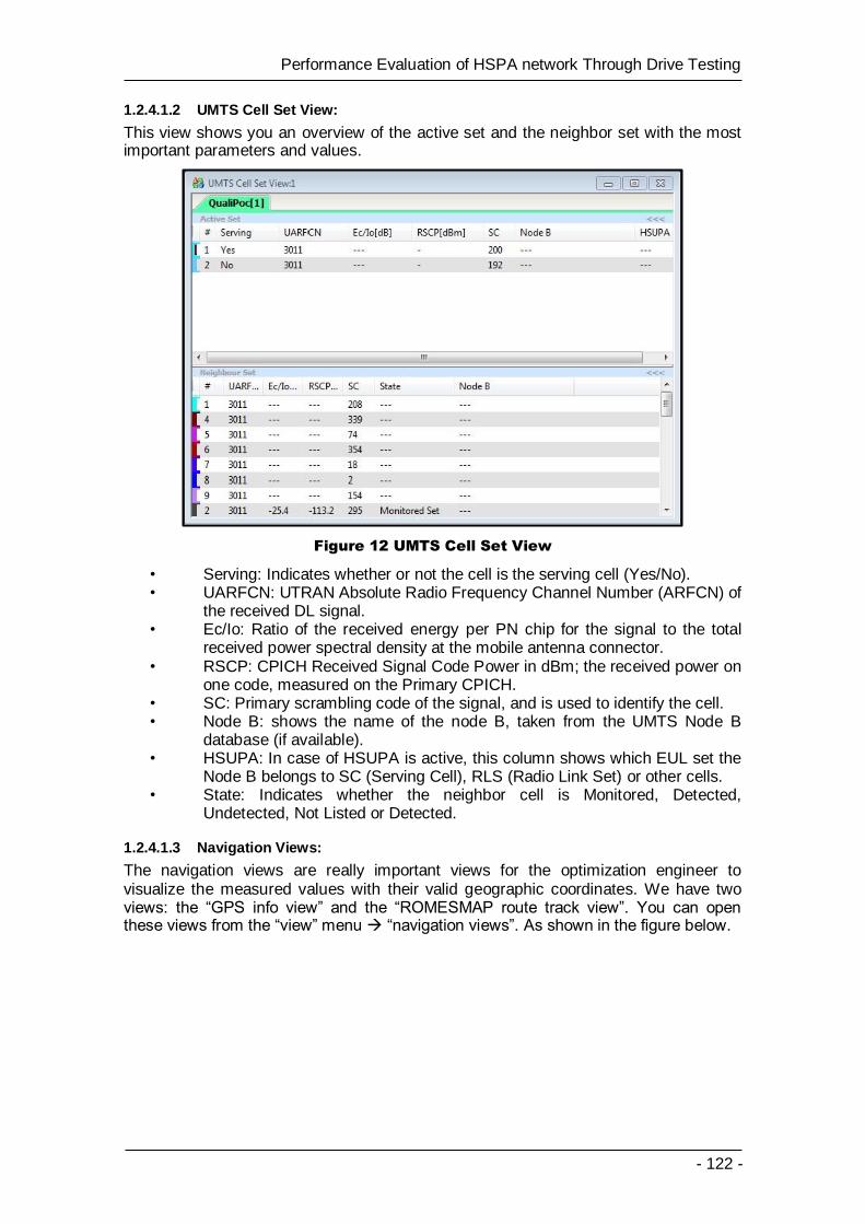
- 122 -


1.2.4.1.2 UMTS Cell Set View:

This view shows you an overview of the active set and the neighbor set with the most important parameters and values.

Figure 12 UMTS Cell Set View

• Serving: Indicates whether or not the cell is the serving cell (Yes/No). • UARFCN: UTRAN Absolute Radio Frequency Channel Number (ARFCN) of

the received DL signal. • Ec/Io: Ratio of the received energy per PN chip for the signal to the total

received power spectral density at the mobile antenna connector. • RSCP: CPICH Received Signal Code Power in dBm; the received power on

one code, measured on the Primary CPICH. • SC: Primary scrambling code of the signal, and is used to identify the cell. • Node B: shows the name of the node B, taken from the UMTS Node B

database (if available). • HSUPA: In case of HSUPA is active, this column shows which EUL set the

Node B belongs to SC (Serving Cell), RLS (Radio Link Set) or other cells. • State: Indicates whether the neighbor cell is Monitored, Detected,

Undetected, Not Listed or Detected.

1.2.4.1.3 Navigation Views:

The navigation views are really important views for the optimization engineer to visualize the measured values with their valid geographic coordinates. We have two views: the “GPS info view” and the “ROMESMAP route track view”. You can open these views from the “view” menu “navigation views”. As shown in the figure below.

- 123 -


Figure 13 Navigation Views

1.2.4.1.3.1 GPS Info View:

The GPS info view shows you the recorded GPS information (longitude, latitude, altitude, compass heading, speed, and the detected GPS satellites with the relative quality of the received GPS signal…etc.)

Figure 14 GPS Info View

1.2.4.1.3.2 ROMESMAP route track view:

The route track view shows the measured data with its projection on a map view (the map can be loaded and positioned into the view) according to the coordinates corresponding to each data sample. This view contains several sections or parts that will be listed and shown in the figure below:

- 124 -


Figure 15 ROMES MAP route track view

• The map view: is the middle section and contains the main display area for the route track of the measurement. And this display view is composed of different layers, each layer shows different “map” to create the overall map view that you can see. For example the lowest layer can be the map of the European countries with different colors, the layer above this one can be a detailed map of Barcelona area, and then a layer for the BTS locations, also one layer for the route driven by the test mobile, also one layer for the signal you want to display like for example the RSCP signal, and there is one layer also for the event map and so on…

Note: the BTS locations layer will not be shown without the “BTS information file” that can be loaded into ROMES and contains all the information about the BTS such as location (coordinates), azimuth, cells IDs, scrambling codes and so on…

• Toolbar (the upper section): contains some tools to modify some functions in the map view, like zooming, changing the order of the layers and moving them, adding routes from measurement files, auto panning on/off function and so on…

• Easy configuration (the left section): contains fast access buttons for the visibility of BTS info, color and technology specific features. Requires the BTS information file to work.

• The footer (bottom section): shows the position of the cursor, the current scale factor and the geographical coordinates of the current measurement point.

• Tree view (the right section): contains all the loaded layers.

Before being able to load a map into ROMES you need to create the map files with the extension “.tab” using the MapInfo software.

First thing you need to do is to download the map shape file from this this link below:

http://downloads.cloudmade.com/europe/southern_europe/spain/cataluna#downloads_breadcrumbs

In our case we will download the shape file for Catalunya map:

So you have to download the file cataluna.shapefiles.zip that you will find at the bottom of the page as shown in the figure below:



http://downloads.cloudmade.com/europe/southern_europe/spain/cataluna/cataluna.shapefiles.zip

- 125 -


Figure 16 Catalunya Shape file download link

After downloading this file and extracting it, then the MapInfo needs to be used to create the tab files.

When you open the MapInfo software, you choose from the “file” menu the “new table” option and a menu like in the figure below will be opened:

Figure 17 New Table Menu

By pressing “create”, a new window named “new table structure” will be opened, that will give you the option to add a file like in the figure shown below:

- 126 -


Figure 18 new table structure

Then from the “projection” you need to choose the type of projection and in our case is the first option “Longitude/Latitude” as shown below:

Figure 19 Projection Type choosing

After pressing ok, you need to save the date base you created in any location you want like in the figure below:

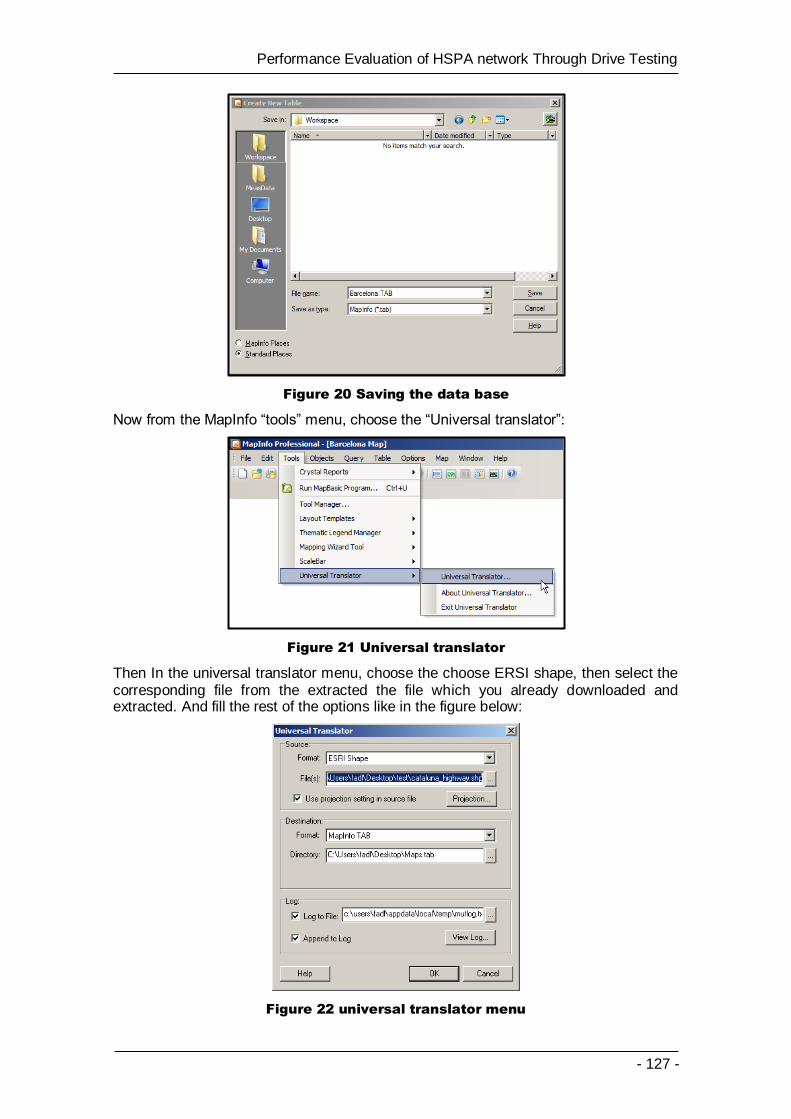
- 127 -


Figure 20 Saving the data base

Now from the MapInfo “tools” menu, choose the “Universal translator”:

Figure 21 Universal translator

Then In the universal translator menu, choose the choose ERSI shape, then select the corresponding file from the extracted the file which you already downloaded and extracted. And fill the rest of the options like in the figure below:

Figure 22 universal translator menu

- 128 -


As for the projection option you have to choose the same type of projection as you did before. And finally when you press ok, you will have the map files with “.TAB” extension that can be opened by the ROMES and loaded into the map view.

Loading a map: in order to load a map, in this lab you are provided with maps files for Catalunya area with the extension “.tab”. They contain several layers to be loaded into the ROMES. Follow the instructions below:

By pressing with the right button anywhere in the map view and then to "maps” “load MapInfo map” “create map”.

Figure 23 loading a map (1)

A layer control window will be opened that allow you to add layers that have the extension “.tab”. After adding the tab file that contains the map you want to add you select ok and it will be loaded to the ROMES map view.

Figure 24 Layer Control

- 129 -


Figure 25 loading a map (2)

1.2.4.1.3.3 Displaying a specific signal on the map view:

If you want to display a certain signal on the map view you need to load this signal into the view by pressing with the right button of the mouse in any place inside the view and choose the configure option. Then inside the configuration menu you will find a list of the available signals to be loaded. After choosing what signal you want to display, you press ok then you will find that a layer of this signal is added to the map with a legend to define the colors with corresponding values. In the figures below you will find an example of loading an RSCP signal to the map view.

Figure 26 Map view Configuration (1)

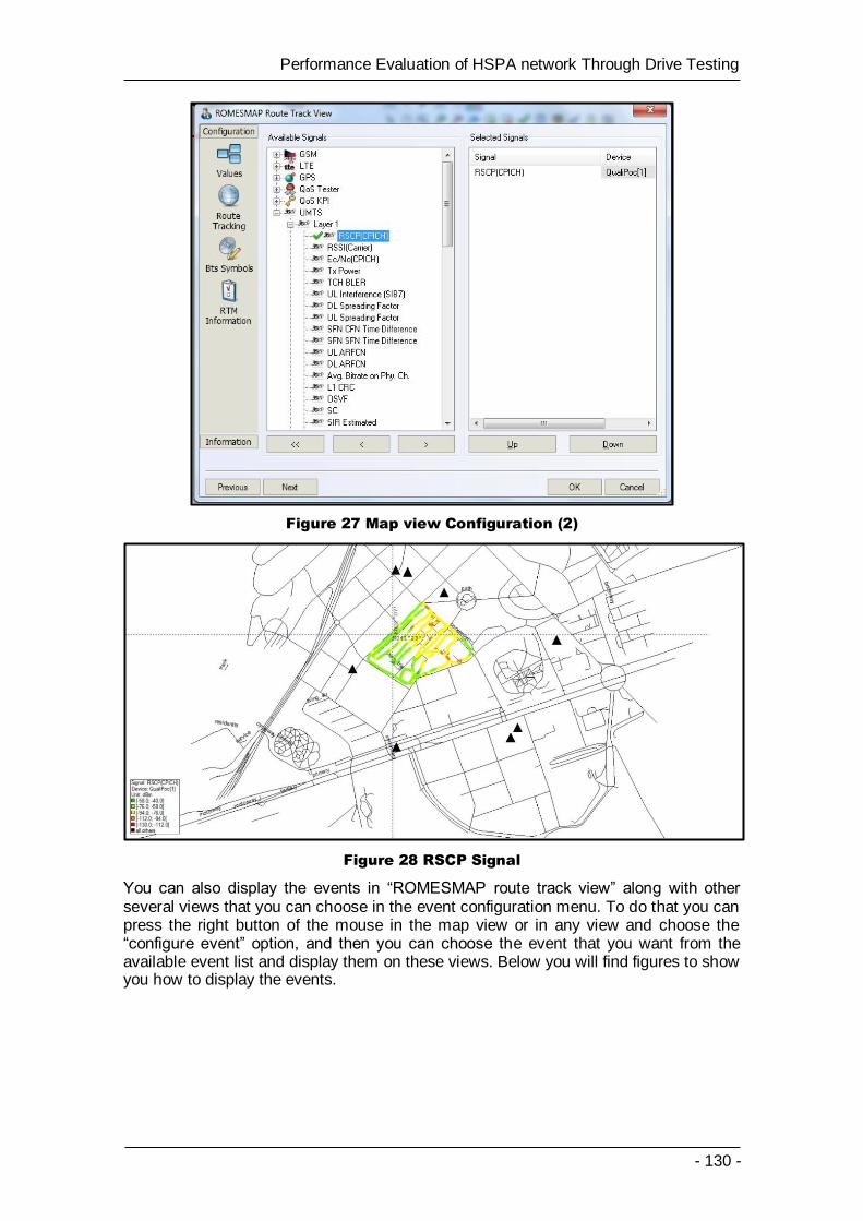
- 130 -


Figure 27 Map view Configuration (2)

Figure 28 RSCP Signal

You can also display the events in “ROMESMAP route track view” along with other several views that you can choose in the event configuration menu. To do that you can press the right button of the mouse in the map view or in any view and choose the “configure event” option, and then you can choose the event that you want from the available event list and display them on these views. Below you will find figures to show you how to display the events.

- 131 -


Figure 29 Events Configuration (1)

Figure 30 Events Configuration (2)

And the result will be like in the figure below:

- 132 -


Figure 31 Soft Handover events Display

1.2.4.1.4 Basic Views:

The basic views are used to analyze data from various sources and display results in different ways. These views do not depend on the type of the measurement that being replayed or recorded. You can display any parameter you want in different views for better analyzing. Below you will find an example of analyzing the RxLev Sub and RxQual Sub for a GSM network test and display the values in “2D Chart View”. You can do that from the “View” menuBasic View 2D Chart View. And then you press with right button anywhere in the view and press on “Configure” and then select the parameter you want (in this example it is the RxLev Sub and RxQual Sub under “Server Report” tap under “GSM” tap as shown in the figures below:

Figure 32 Basic views menu

- 133 -


Figure 33 2D chart view Configuration

Figure 34 2D Chart view

The rest of the views can be configured in the same manner as shown before, and can be used to have different look on the data under analysis.

To be more familiar with the ROMES R&S tool, in the next section you will find three practical exercises for three different tests measurements. The measurement files for these 3 tests will be the same measurement files that you have created in the first lab exercise.

1.3 Practical Exercises:

1.3.1 Analysis of Idle Monitoring Tests

Open the measurement file for the idle monitoring test created by you using QualiPoc in the first lab exercise and start observing the main views.

Question #1: open the 3GPP overview view from the mobile views and find out where you can see the technology that is being tested? Where can you see the serving cell ID and the Scrambling code of that cell?

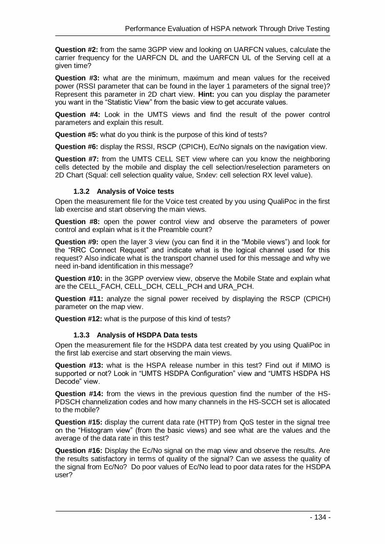
- 134 -


Question #2: from the same 3GPP view and looking on UARFCN values, calculate the carrier frequency for the UARFCN DL and the UARFCN UL of the Serving cell at a given time?

Question #3: what are the minimum, maximum and mean values for the received power (RSSI parameter that can be found in the layer 1 parameters of the signal tree)? Represent this parameter in 2D chart view. Hint: you can you display the parameter you want in the “Statistic View” from the basic view to get accurate values.

Question #4: Look in the UMTS views and find the result of the power control parameters and explain this result.

Question #5: what do you think is the purpose of this kind of tests?

Question #6: display the RSSI, RSCP (CPICH), Ec/No signals on the navigation view.

Question #7: from the UMTS CELL SET view where can you know the neighboring cells detected by the mobile and display the cell selection/reselection parameters on 2D Chart (Squal: cell selection quality value, Srxlev: cell selection RX level value).

1.3.2 Analysis of Voice tests

Open the measurement file for the Voice test created by you using QualiPoc in the first lab exercise and start observing the main views.

Question #8: open the power control view and observe the parameters of power control and explain what is it the Preamble count?

Question #9: open the layer 3 view (you can find it in the “Mobile views”) and look for the “RRC Connect Request” and indicate what is the logical channel used for this request? Also indicate what is the transport channel used for this message and why we need in-band identification in this message?

Question #10: in the 3GPP overview view, observe the Mobile State and explain what are the CELL_FACH, CELL_DCH, CELL_PCH and URA_PCH.

Question #11: analyze the signal power received by displaying the RSCP (CPICH) parameter on the map view.

Question #12: what is the purpose of this kind of tests?

1.3.3 Analysis of HSDPA Data tests

Open the measurement file for the HSDPA data test created by you using QualiPoc in the first lab exercise and start observing the main views.

Question #13: what is the HSPA release number in this test? Find out if MIMO is supported or not? Look in “UMTS HSDPA Configuration” view and “UMTS HSDPA HS Decode” view.

Question #14: from the views in the previous question find the number of the HS-PDSCH channelization codes and how many channels in the HS-SCCH set is allocated to the mobile?

Question #15: display the current data rate (HTTP) from QoS tester in the signal tree on the “Histogram view” (from the basic views) and see what are the values and the average of the data rate in this test?

Question #16: Display the Ec/No signal on the map view and observe the results. Are the results satisfactory in terms of quality of the signal? Can we assess the quality of the signal from Ec/No? Do poor values of Ec/No lead to poor data rates for the HSDPA user?

- 135 -


Question #17: what is the parameter that represents the channel condition and on which physical channel is reported?

Question #18: Explain the Scheduled throughput, the requested throughput, Delta throughput and MAC throughput that you can see from the UMTS HSDPA Performance view

1.3.4 Analysis of Multiple-tests (Multi-RAB test)

Open the measurement file for the Multi-RAB test created by you using QualiPoc in the first lab exercise and start observing the main views.

Question #19: what is the meaning of multi-RAB and why is important to have this kind of tests?

Question #20: According to a single RAB HSDPA data test did you find something changed regarding the data rate or not?

Question #21: why is it important to analyze specifically a multi-RAB test if we already analyzed a test for a voice call and a test for HSDPA data?

- 136 -


ANNEX D: ROMES R&S

Tutorial Answers


- 137 -


Table of Content

1. ANNEX D: ROMES R&S Tutorial Answers ..................... - 138 -

1.1 Practical exercises answers .................................................................... - 138 -

1.1.1 Analysis of Idle Monitoring Tests ................................................... - 138 -

1.1.2 Analysis of Voice tests .................................................................. - 142 -

1.1.3 Analysis of HSDPA Data tests ....................................................... - 145 -

1.1.4 Analysis of Multiple-tests (Multi-RAB test) ...................................... - 150 -

- 138 -


1. ANNEX D: ROMES R&S TUTORIAL ANSWERS

1.1 Practical exercises answers

1.1.1 Analysis of Idle Monitoring Tests

Open the measurement file for the idle monitoring test created by you using QualiPoc in the first lab exercise and start observing the main views.

Question #1 open the 3GPP overview view from the mobile views and find out where you can see the technology that is being tested? Where can you see the serving cell ID and the Scrambling code of that cell?

Answer: from observing the 3GPP overview view we can clearly that the technology being tested is UMTS, and the serving cell id and SC can be viewed also from the same view as shown in the figure below:


Question #2: from the same 3GPP view and looking on UARFCN values, calculate the carrier frequency for the UARFCN DL and the UARFCN UL of the Serving cell at a given time?

Answer: the carrier frequency can be calculated from the following equation:

Question #3: what are the minimum, maximum and mean values for the received power (RSSI parameter that can be found in the layer 1 parameters of the signal tree)? Represent this parameter in 2D chart view. Hint: you can you display the parameter you want in the “Statistic View” from the basic view to get accurate values

Answer: to find these values in an accurate manner we can represent the RSSI parameter in the statistic view from the basic views as shown in the figure below:

Opening the statistic view: “view” menu Basic Views statistic view.

- 139 -


Figure 36 statistic view

Configuring the view: right button anywhere on the view “configure”

Figure 37 statistic view configuration

The result:

Figure 38 RSSI Statistics

- 140 -


As for representing the RSSI parameter in 2D chart view, we can follow the same procedure but instead we choose the 2D chart view

Figure 39 2D Chart (RSSI Parameter)

Question #4 Look in the UMTS views and find the result of the power control parameters and explain this result.

Answer: from the “view” menu mobile views UMTS UMTS Power control view

Figure 40 UMTS Power control view

The reason why we don’t have any data in the power control view is because the mobile is in idle monitoring mode and it is not initiating any activity with the network.

Question #5: what do you think is the purpose of this kind of tests?

Answer: The purpose of the idle monitoring test is to analyze the coverage issues, cell reselection process, and location area update procedures.

- 141 -


Question #6: display the RSSI, RSCP (CPICH), Ec/No signals on the navigation view.

Answer: we can configure the map with the parameters that we want to show like any other view.

Figure 41 RSCP (CPICH) Signal

Figure 42 Ec/No (CPICH) Signal

Figure 43 RSSI (Carrier) Signal

- 142 -


Question #7: from the UMTS CELL SET view where can you know the neighboring cells detected by the mobile and display the cell selection/reselection parameters on 2D Chart (Squal: cell selection quality value, Srxlev: cell selection RX level value).

Answer: we can find neighboring cells set from UMTS tab and in the “UMTS Cell Set View” which is opened automatically as shown in the figure below:

Figure 44 UMTS Cell Set View

We can also display the cell selection/reselection parameters (Squal: cell selection quality value, Srxlev: cell selection RX level value) on any basic view by configuring that view on these parameters.

Figure 45 Squal and Srxlev on 2D Chart

1.1.2 Analysis of Voice tests

Open the measurement file for the Voice test created by you using QualiPoc in the first lab exercise and start observing the main views.

Question #8: open the power control view and observe the parameters of power control and explain what is it the Preamble count?

- 143 -


Answer: now that the mobile is in connected state, we will see power control parameters because it is mandatory in UMTS system.

Figure 46 UMTS Power control view

The preamble is used in the Open loop power control (in the first access). In this mechanism to reduce the risk of increased interference we use the power ramping mechanism, in which the terminal starts with lower transmitted power than the estimated one in the open loop and transmits a preamble and waits for a certain time to see if the system can detect this level of power and send a response. If there no response the terminal increases the power a little bit and tries again until the system acknowledges that the preamble has been detected, and then after that the terminal starts to send data at that certain level of power.

Question #9: open the layer 3 view (you can find it in the “Mobile views”) and look for the “RRC Connect Request” and indicate what is the logical channel used for this request? Also indicate what is the transport channel used for this message and why we need in-band identification in this message?

Answer: The logical channel used for this request is CCCH (common control channel) which is necessary in the first access to create RRC connection, as for the transport channel used is RACH (random access channel) and we need in-band identification because RACH is shared by several users and necessarily within the headers of the message sent through this channel we need some fields to discriminates among users.

- 144 -


Figure 47 Layer 3 Messages View

Question #10: in the 3GPP overview view, observe the Mobile State and explain what are the CELL_FACH, CELL_DCH, CELL_PCH and URA_PCH.

Answer:


Depending on the type of connection and the traveling speed, the UE may be in one of several different states. This is handled by the RRC states, controlled by the RNC. In Idle mode the UE has no active connections. In Connected mode the UE may be in one of four RRC states:

- 145 -


• The CELL_FACH (Forward Access Channel) state is used for communication over common channels with limited bandwidth, e.g. IMSI Attach and LU

• The CELL_DCH (Dedicated Channel) state is used for communication over allocated dedicated channels like voice call and data transmission. In this state the UTRAN will perform handovers for CS QoS and Cell Update for PS QoS.

• The CELL_PCH (Paging Channel) and URA_PCH states are used when there is no data to send. The UE will only listen to the Paging Channel thus minimizing battery load. In the Cell PCH state the UE will perform Cell Updates whereas in the URA_PCH state the UE performs the less frequent UTRAN Registration Area (URA) Updates. The advantage of the latter is increased power savings and the sacrifice is that paging is required. E.g. URA_PCH is preferred to CELL_PCH when the UE is moving at high speed to minimize frequency of location updating procedures.

Question #11: analyze the signal power received by displaying the RSCP (CPICH) parameter on the map view.

Answer: we can configure the 2D chart with RSCP (CPICH) signal in the same way as we seen before.

Figure 49 RSCP (CPICH) Signal on map view

Question #12: what is the purpose of this kind of tests?

Answer: the purpose of the voice test is to analyze the signal quality, handover procedures, drop calls, power control parameters, and call setup procedures and so on…

1.1.3 Analysis of HSDPA Data tests

Open the measurement file for the HSDPA data test created by you using QualiPoc in the first lab exercise and start observing the main views.

Question #13: what is the HSPA release number in this test? Find out if MIMO is supported or not? Look in “UMTS HSDPA Configuration” view and “UMTS HSDPA HS Decode” view.

Answer: we can see the HSPA type from the “UMTS HSDPA Configuration” view which shows the configuration of the DL HSDPA channels received by the test mobile,

- 146 -


the UL HS-DPCCH, the DL HS-SCCHs, and the active HARQ processes. You can open this view from the “view” menu Mobile views HSDPA views UMTS HSDPA Configuration. See figure 50.

To know if MIMO is supported or not, there are some ways to do that and the easiest one for example is to look in the “UMTS HSDPA HS Decode” view which is opened automatically. This view shows the status of the HS-SCCH demodulation and the decoded HS-SCCH information. And it is split in two parts with three sections each. In MIMO case, the two parts of the view are filled:

• The upper part reflects the state of the first MIMO path (first carrier). • The lower part reflects the state of the second MIMO path (secondary

carrier).

See the figures below.

Figure 50 UMTS HSDPA Configuration view

Figure 51 UMTS HSDPA HS Decode view

- 147 -


Question #14: from the views in the previous question find the number of the HS-PDSCH channelization codes and how many channels in the HS-SCCH set is allocated to the mobile?

Answer: from the same “UMTS HSDPA HS Decode” view we can see “#HS-DSCH codes” parameter that tell us the Number of HS-(P)DSCH channelization codes in the range between 1 and 15.

To know how many channels in the HS-SCCH set is allocated to the mobile we can look in the “UMTS HSDPA Configuration” view opened before, under the SCCH information tab and find how many channels are enabled

Question #15 display the current data rate (HTTP) from QoS tester in the signal tree on the “Histogram view” (from the basic views) and see what are the values and the average of the data rate in this test?

Answer: we can open the Histogram view from the basic views and configure it for the “Current Data Rate (HTTP)” parameter that can be found as show in the figure below:

Figure 52 Statistic Histogram Configuration

Figure 53 current data rate (HTTP)

Question #16: Display the Ec/No signal on the map view and observe the results. Are the results satisfactory in terms of quality of the signal? Can we assess the quality of

- 148 -


the signal from Ec/No? Do poor values of Ec/No lead to poor data rates for the HSDPA user?

Answer: The CPICH Ec/No measurements collected during HSDPA Transmission could mask the true radio conditions, because while the HSDPA session adds to the overall load of the cell which is taken into consideration during the computation of Ec/No, this computation does not necessarily give the TRUE radio conditions. So as an alternative to the Ec/No in High Speed Sessions the parameter CQI (Channel Quality Indicator) was added to give the true radio conditions to be reported to the NodeB.

That means, in a live network where resources of a cell are shared between many users, and Interference from other cells also plays its part, the Ec/No will always give a FALSE value for an HSDPA user. And it will show a very poor value. And that’s why we use CQI. And while SINR is used to evaluate the channel quality as observed by the receiver, the UE calculate the CQI value to be reported to the NodeB via a linear mapping as shown below:

[ ]

The UE periodically sends a CQI to the serving HS-DSCH cell on the uplink high-speed dedicated physical control channel (HS-DPCCH). These CQI values are used by the link adaptation algorithm at the Node-B so that every CQI value reported corresponds to the Transport Block Size (TBS) that can be granted on a particular Modulation type and Number of codes (CQI to TBS mapping tables).

The HSDPA system defines a different CQI mapping table for different categories of UEs. The category is determined according to the capability of UE.

So the system is essentially calculating the Data Rate to be scheduled to the user based on CQI reports and BLER which it receives from the UE.

[ ] [ ]

[ ]⁄

In the figures below you will find the Ec/Io and CQI values shown on the map view. You can see clearly that the Ec/No signal is always poor in this test while the CQI gives the true radio conditions.

Figure 54 Ec/No CPICH Signal

- 149 -


Figure 55 CQI Parameter

Question #17: what is the parameter that represents the channel condition and on which physical channel is reported?

Answer: from the "UMTS HSDPA UL HS-DPCCH View" shows the CQI values reported by the test mobile in the last 100 HSDPA sub frames. In the network, the Channel Quality Indicator (CQI) represents the Channel condition and is transmitted on the UL High Speed Dedicated Physical Control Channel (HS-DPCCH), which is a fixed rate channel with a spreading factor of 256. The first slot of each UL HS-DPCCH sub frame contains the ACK/NACK messages; the following two slots carry the CQI. See figure below.

Figure 56 UMTS HSDPA UL HS-DPCCH View

Question #18: Explain the Scheduled throughput, the requested throughput, Delta throughput and MAC throughput that you can see from the UMTS HSDPA Performance view.

Answer: The “Requested throughput” is the data throughput that the mobile requests according to the measured channel quality. The requested throughput is calculated from the CQI messages that the mobile transmits on the UL HS-DPCCH. However the “Scheduled throughput” is the data throughput that the network uses according to the requests (CQI messages) from the mobile. The results are analogous to the “Requested Throughput” results.

- 150 -


The "Delta" throughput is the difference between the scheduled and the requested throughputs. The results are analogous to the "Requested Throughput" results. If there is no network congestion, the delta results are close to zero.

The HS-"MAC Layer" throughput is the actual DL data throughput achieved. The MAC throughput depends on the scheduled throughput and the percentage of data blocks that the network has to re-transmit ("HARQ Retransmission Rate").

We can find these throughputs in the “UMTS HSDPA Performance” view

Figure 57 UMTS HSDPA Performance view

1.1.4 Analysis of Multiple-tests (Multi-RAB test)

Open the measurement file for the Multi-RAB test created by you using QualiPoc in the first lab exercise and start observing the main views.

Question #19: what is the meaning of multi-RAB and why is important to have this kind of tests?

Answer: Radio access bearers (RABs) are specific data flow conduits that identify the service the AS (Access Stratum) provides to the NAS (Non Access Stratum) for transfer of user data between the UE (User Equipment) and the CN (Core Network). In UMTS, there is a one-to-one mapping of RABs to PDPs. So multi-RAB capability gives the possibility to have two or more simultaneous RABs to support simultaneous communication over the radio access network with multiple service access points.

Multi-RAB test is important because nowadays smartphones assume an always on IP connection with applications automatically initiating a connection to check for updates. And the users however are oblivious as they make voice calls while their phone continues to make these background data connections.

Question #20: According to a single RAB HSDPA data test did you find something changed regarding the data rate or not?

Answer: For Rel 99 multi-RABs, the radio bearers are multiplexed on MAC-d level into one single dedicated transport channel (DCH), with a maximum rate of 8, 16, 64, 128 or 384 Kbps for both downlink and uplink. The maximum bit rate is shared by the two RABs, meaning the sum of the instantaneous bit rates on the bearers transmitted in a TTI (Transmission Time Interval) is less than or equal to the maximum bit rate on the DCH. The transport channel is shared, and also has lower transport formats in order to adapt to lower data rates when there is less data to transmit.

- 151 -


For HSDPA Multi-RABs, there is no multiplexing on the MAC-d level for the downlink. Instead, the radio bearers are carried as different MAC-d flows down to the RBS, where the data is put into separate priority queues for scheduling on the HS-DSCH (Downlink Shared Channel used in HSDPA). The available HS-DSCH bandwidth is shared between the various flows.

Question #21: why is it important to analyze specifically a multi-RAB test if we already analyzed a test for a voice call and a test for HSDPA data?

Answer: Due to the complex interaction of voice and data services, some issues arise when using multi-RAB services like:

• Dropped voice calls and data sessions on certain handset models that have problems with specific RAB types.

• IRAT (Inter-radio access technology) handovers to GSM become complicated especially if dual transfer mode isn’t supported.

- 152 -


ANNEX E: KPI in Different

Technologies

- 153 -


Table of Content

1. ANNEX E: KPI in different technologies ......................... - 154 -

1.1 KPI in GSM ............................................................................................ - 154 -

1.1.1 Call Setup Success Rate (CSSR) .................................................. - 154 -

1.1.2 Call Drop Rate (CDR) ................................................................... - 154 -

1.1.3 Call Success Rate (CSR) .............................................................. - 154 -

1.1.4 Handover Success Rate (HOSR) .................................................. - 154 -

1.1.5 Location Area Update Success (LAUSR) ....................................... - 154 -

1.1.6 Call Setup Time (CST) .................................................................. - 154 -

1.1.7 Downlink Signal Strength (RxLev) ................................................. - 155 -

1.1.8 Downlink Signal Quality (RxQual) .................................................. - 156 -

1.1.9 SQI (Speech Quality Index) ........................................................... - 156 -

1.1.10 Time Advance (TA) ....................................................................... - 156 -

1.2 KPI in UMTS .......................................................................................... - 157 -

1.2.1 RAB Establishment Success Rate (RABESR) ................................ - 157 -

1.2.2 RRC Connection Establishment Success Rate (RRCCESR) .......... - 158 -

1.2.3 UTRAN Service Access Success Rate (USAR) .............................. - 158 -

1.2.4 GERAN Service Access Success Rate for CS Domain (GASRCS) . - 158 -

1.2.5 UMTS PDP Context Activation Success Rate (UPDPCASR) .......... - 158 -

1.2.6 UMTS Switched Call Success Rate (USASR) ................................ - 158 -

1.2.7 RAB Abnormal Release Rate (RARR) ........................................... - 159 -

1.2.8 Soft Handover Success Rate (SHOSR) ......................................... - 159 -

1.2.9 Outgoing Intra-system Hard Handover Success Rate (HHOSR) ..... - 159 -

1.2.10 Outgoing Inter RAT Handover Success Rate for PS Domain (IRATHOSR-PS) - 159 -

1.2.11 Percentage of Established RABs, TotalPS (RabEstabTotalPS)....... - 160 -

1.2.12 UTRAN Cell Availability (CellAvailability) ....................................... - 160 -

1.3 KPI in LTE .............................................................................................. - 160 -

1.3.1 Initial E-RAB establishment success rate (IRESR) ......................... - 160 -

1.3.2 Added E-RAB establishment success rate (ARESR) ...................... - 161 -

1.3.3 E-RAB Release Rate (RRR).......................................................... - 161 -

1.3.4 Data Radio Bearer Throughput (DRBTHP) .................................... - 162 -

1.3.5 Data Radio Bearer Latency (DRB latency) ..................................... - 162 -

1.3.6 E-UTRAN Packet Loss (EUPL) ..................................................... - 162 -

1.3.7 Partial cell availability (node restarts excluded) .............................. - 163 -

1.3.8 E-UTRAN Mobility Success Rate (EMSR)...................................... - 163 -

- 154 -


1. ANNEX E: KPI IN DIFFERENT TECHNOLOGIES

1.1 KPI in GSM

1.1.1 Call Setup Success Rate (CSSR)

Call setup success rate gives a measure of the successful calls that reach its destination. This counter do not count the failures during the call, thus, drop Calls are not included in this statistic. Call Setup Success Rate will be calculated from the drive test results "log files" via the following equation:

1.1.2 Call Drop Rate (CDR)

This KPI will count the abnormally disconnected calls, and do a ratio between it and the total numbers of calls. CR will be calculated by counting the number of the calls established successfully and the number of calls which were dropped.

1.1.3 Call Success Rate (CSR)

If we want to have good overview knowledge about the network health, we can use this KPI which combine the CSSR and the CDR in one figure, in other words how many established calls started and finished appropriately.

1.1.4 Handover Success Rate (HOSR)

It will indicate the ratio for the successful Handover over all the handover attempts, and it can be calculated via the equation:

1.1.5 Location Area Update Success (LAUSR)

We can find out about the Location Area Update Success rate by applying the following equation, the ratio between the number of LAU failures and the number of the total LAU will indicate the failing percentage, so its reverse will indicate the successful percentage. Normally LAUSR must be 100% in any healthy network.

1.1.6 Call Setup Time (CST)

It is the time needed to establish a successful call (ending when the TCH is activated and ready to use).

- 155 -


This time varies depending on the destination receiver; usually we need less time to setup a call from a mobile device to a fix phone (around 3s) than from mobile to another (around 7s), and that because of the additional time that must be spent during the paging procedure in the second case, which is about 2 ~3s (depending on factors such as the paging channel load, the paging repetition timer, the core hardware delay … etc.). An example for the CST is shown in figure 1.

Figure 1 Call setup time (GSM)

From the figure above, we can see how the CST varies from area to another and how the CST to a fixed phone (represented in yellow) is lower than the CST in case the destination were a mobile device (represented in red).

1.1.7 Downlink Signal Strength (RxLev)

The down links signal strength is the received signal level (RxLev), we can measure this value in the idle mode or/and the dedicated mode. Weak RxLev measurements indicate a high possibility of low network performance. Each operator/vendor decides how to divide the RxLev values into different levels according to their target, the following table 1 shows an example for an RxLev criteria decided by MTN.

Table 1 RxLev criteria

- 156 -


1.1.8 Downlink Signal Quality (RxQual)

The downlink signal quality is the received quality level (RxQual) from the BTS; this term is related to the BER in general and it is sensitive to factors such as the signal level (RxLev), the interference and the receiver characteristics. In GSM technology, RxQual has a value within the range 0 to 7, where 0 is the best and 7 is the worst. Clearly this KPI is use only in a dedicated mode. The following example, table 2, is MTN RxQual criteria:

Table 2 RxQual criteria

But we need to set some threshold distances where the bad quality spots could be considered as a problem, which means we say that we are facing some quality problem in a specific spot, just if the spot is near enough to the base station and it is not usual to have bad quality there. So MTN also consider the following distances as a threshold distances when studying the RxQual. Dense Urban: 140 m City: 225 m Highway: 335 m

1.1.9 SQI (Speech Quality Index)

The sub-KPI, SQI (Speech Quality Index) calculates approximately the speech quality in the network as offered to the listener (the subscriber). The distributing of both speech codec used in GSM such as AMR (FR and HR) and EFR within the network will affect the calculation of the SQI along with many other terms such as BER, FER (frame error rate), HO … etc. SQI values are divided from -20 ~ 30, a possible criterion is shown in table 3. One of the best things to do to improve the SQI is by reduce the unnecessary handovers in the network, and by removing the interference which could be found on some bad spots.

SQI SQI Criteria

20<=x<=30 Excellent

10<=x<20 Fair

0<=x<10 Poor

(-10)<=x<(0) Bad

(-20)<=x<(-10) Very Bad

Table 3 SQI criteria

1.1.10 Time Advance (TA)

The main purpose of using TA value in GSM is to reach the required synchronization between the MS and the base station in the UL case. The TA value is related relatively to the distance between the base station and the MS, if the distance changes, TA will change also. By using TDMA technology in GSM, multiple users will share the same frequency to transmit the data periodically but at different time within the time slot (TS),

- 157 -


and because of the different distances from the base station for every MS, we need to use the TA value to detect this distance and delay the transmission in a correct way. TA takes a value between 0 and 63; each step in this range represents an additional period for the symbol (3.69 microseconds). And by considering the velocity of the electromagnetic waves we can find that one TA step represents a change in the round-trip distance of about 1,100 meters. This means that each TA value is equal to 550m. There are no criteria for the TA; we use the "log files" to find out how the TA is distributed within the network, later we can use this information when analyzing some events that could occur in the network. Table 4 shows the TA distributions in the same PLMN for two different operators.

Operator Operator 1 Operator 2

TA % %

0-1 49.53% 57.36%

1-2 37.94% 32.94%

2-3 6.84% 6.65%

3-4 2.50% 1.22%

4-6 2.60% 1.51%

6-9 0.19% 0.18%

9-12 0.19% 0.07%

12-64 0.21% 0.08%

Table 4 TA distribution in different operators

As we can notice from table 4, TA values beyond 4 are not commonly used.

1.2 KPI in UMTS ‎[16]

1.2.1 RAB Establishment Success Rate (RABESR)

This KPI is included in the accessibility category. To evaluate the accessibility across UTRAN we need to calculate the percentage of the successful RAM establishments within the UTRAN by the following equation:

As we notice from the equation we need to include both statistics from CS and PS, and that because RAB provides services for both domains (voice call, web services), so this KPI shows the readiness of the UTRAN to give access to all of its services. Furthermore we can divide this KPI and use only a part of it, for example if we need to evaluate the RAB across UTRAN only for a voice calls or only for PS services we can use the same equation mentioned above but with eliminating the CS or the PS part from it.

- 158 -


1.2.2 RRC Connection Establishment Success Rate (RRCCESR)

There are two kinds of RRC connection. One kind is related to service access, the other kind is not related to service, such as related to location update, cell update, network registration etc. first kind of RRC connection can be used to evaluate service accessibility across UTRAN, second one can be used to evaluate RNC or cell admission capacity for MS and/or system load. The following equation shows that we can obtain this KPI by dividing the successful RAB establishment over the attempts:

1.2.3 UTRAN Service Access Success Rate (USAR)

This KPI describes the ratio of all successful UTRAN access to UTRAN access attempts for UTRAN network and is used to evaluate service accessibility provided by UTRAN. Successful RRC set up repetition and/or cell re-selections during RRC setup should be excluded, namely only service related RRC setup should be considered.

Where RABESR is: RAB Establishment Success Rate for all RAB types and by RRC Connection Establishment in this equation we mean only the RRC Connection Establishment Rate for UTRAN access purposes.

1.2.4 GERAN Service Access Success Rate for CS Domain (GASRCS)

This KPI describes the ratio of all successful GERAN access to GERAN access attempts for a GERAN network. This KPI will be use to evaluate service accessibility provided by GERAN. Successful SDCCH set up repetition during SDCCH setup should be excluded, namely only service related SDCCH setup for CS domain should be considered.

This KPI is obtained by the TCH seizures success rate multiplied by the SDCCH setup success rate as in the equation:

1.2.5 UMTS PDP Context Activation Success Rate (UPDPCASR)

This KPI describes the ratio of the number of successfully performed PDP context activation procedures to the number of attempted PDP context activation procedures for UMTS PS core network and is used to evaluate service accessibility provided by UMTS and network performance to provide GPRS.

This KPI is obtained by successful PDP context activation procedures initiated by MS divided by attempted PDP context activation procedures initiated by MS.

1.2.6 UMTS Switched Call Success Rate (USASR)

This KPI is obtained by successful calls for MSC originating and incoming traffic from a given MSC divided by attempted calls for MSC originating calls and incoming calls.

- 159 -


It is necessary to evaluate performance of switched call success rate. If switched call success rate is low, call drop rate will be increased.

1.2.7 RAB Abnormal Release Rate (RARR)

Since the user may complain about a connection released unexpectedly for CS service or unstable for PS service, it is necessary to evaluate CS and/or PS service Retainability provided by UTRAN from user plane aspects, as well as UTRAN reliability and stability should be reflected.

We will calculate RARR by finding the ratio of the number of RAB release requests over the number of successful RAB establishments:

p.s. Also we can divide this KPI to study only the PS or the CS statistics.

1.2.8 Soft Handover Success Rate (SHOSR)

This KPI represent the ratio between the successful soft handovers over the overall soft handovers attempts.

Soft handover is helpful to guarantee service QoS when MS is at the edge of cell coverage. It can be used to evaluate network performance, such as handover decision and handover execution performance. This KPI indicates soft handover performance.

1.2.9 Outgoing Intra-system Hard Handover Success Rate (HHOSR)

This KPI describes the ratio of number of successful outgoing hard handover to the total of the attempted outgoing hard handover.

If outgoing intra-system hard handover is failed, a call maybe drops that user can be perceived. So that it is helpful for network plan and optimization. It can be used to evaluate network performance, such as measurement control, handover decision and handover execution performance … etc.

1.2.10 Outgoing Inter RAT Handover Success Rate for PS Domain (IRATHOSR-PS)

This KPI describes the ratio of number of successful inter RAT handover to the total number of the attempted inter RAT handover from UMTS to GSM for PS domain.

Inter RAT handover is an important function for operators with both GSM and UMTS networks. This KPI can be used to evaluate GSM and UMTS network coverage and stability and reliability performance of inter RAT handover for PS domain. User can perceive service QoS change if this KPI is too low. This KPI is focusing on network and user view.

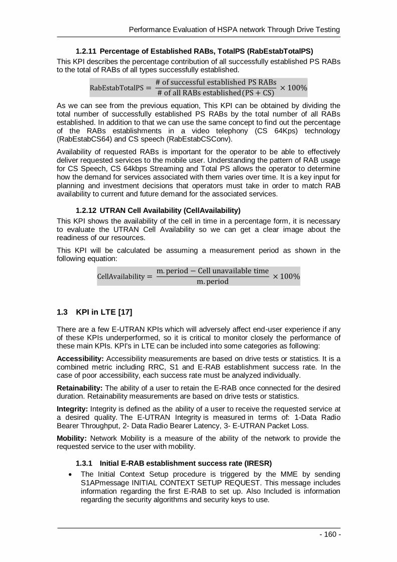
- 160 -


1.2.11 Percentage of Established RABs, TotalPS (RabEstabTotalPS)

This KPI describes the percentage contribution of all successfully established PS RABs to the total of RABs of all types successfully established.

As we can see from the previous equation, This KPI can be obtained by dividing the total number of successfully established PS RABs by the total number of all RABs established. In addition to that we can use the same concept to find out the percentage of the RABs establishments in a video telephony (CS 64Kps) technology (RabEstabCS64) and CS speech (RabEstabCSConv).

Availability of requested RABs is important for the operator to be able to effectively deliver requested services to the mobile user. Understanding the pattern of RAB usage for CS Speech, CS 64kbps Streaming and Total PS allows the operator to determine how the demand for services associated with them varies over time. It is a key input for planning and investment decisions that operators must take in order to match RAB availability to current and future demand for the associated services.

1.2.12 UTRAN Cell Availability (CellAvailability)

This KPI shows the availability of the cell in time in a percentage form, it is necessary to evaluate the UTRAN Cell Availability so we can get a clear image about the readiness of our resources.

This KPI will be calculated be assuming a measurement period as shown in the following equation:

1.3 KPI in LTE ‎[17]

There are a few E-UTRAN KPIs which will adversely affect end-user experience if any of these KPIs underperformed, so it is critical to monitor closely the performance of these main KPIs. KPI's in LTE can be included into some categories as following:

Accessibility: Accessibility measurements are based on drive tests or statistics. It is a combined metric including RRC, S1 and E-RAB establishment success rate. In the case of poor accessibility, each success rate must be analyzed individually.

Retainability: The ability of a user to retain the E-RAB once connected for the desired duration. Retainability measurements are based on drive tests or statistics.

Integrity: Integrity is defined as the ability of a user to receive the requested service at a desired quality. The E-UTRAN Integrity is measured in terms of: 1-Data Radio Bearer Throughput, 2- Data Radio Bearer Latency, 3- E-UTRAN Packet Loss.

Mobility: Network Mobility is a measure of the ability of the network to provide the requested service to the user with mobility.

1.3.1 Initial E-RAB establishment success rate (IRESR)

The Initial Context Setup procedure is triggered by the MME by sending S1APmessage INITIAL CONTEXT SETUP REQUEST. This message includes information regarding the first E-RAB to set up. Also Included is information regarding the security algorithms and security keys to use.

- 161 -


The RBS applies the security information and informs the UE, using the SECURITY MODE COMMAND message. The UE responds with SECURITY MODE COMPLETE. After this point all data between the UE and RBS is encrypted and control signaling is integrity-protected.

Following successful activation of security, the RBS allocates resources for the first Data Radio Bearer. Resources for SRB2 are allocated as well. The RBS configures the UE by sending message RRC CONNECTION RECONFIGURATION.

The UE responds with RRC CONNECTION RECONFIGURATION COMPLETE and the procedure is completed after the RBS has sent INITIAL CONTEXT SETUP RESPONSE to the MME.

[ ]

A = PmRrcConnEstabSucc: A counter for the total number of the successful RCC connection establishments per cell.

B= PmRrcConnEstabAtt: A counter for the total number of RCC connection request attempts per cell.

PmS1SigEstabAtt: A counter for the total number of S1 signaling connection attempts for any establishment cause per cell.

PmS1SigEstabSucc: A counter for the total number of the successful S1 signaling connection establishments per cell.

E= PmZtemporary9: A counter for the total number of RCC connection request attempts that are considered as re-attempts.

PmErabEstabSuccInit: A counter for the total number of the successful Initial E-RAB establishments per cell.

PmErabEstabAttInit: A counter for the total number of Initial E-RAB establishment attempts per cell.

1.3.2 Added E-RAB establishment success rate (ARESR)

Defined as the accessibility success rate for end-user services which is carried by E-RABs included in the E-RAB setup procedure.

[ ]

PmErabEstabSuccAdded: A counter for the total number of the successful added E-RAB establishments per cell.

PmErabEstabAttAdded: A counter for the total number of added E-RAB establishment attempts per cell.

1.3.3 E-RAB Release Rate (RRR)

PmErabRelMmeAct: the total number of E-RAB releases initiated by MME.

PmSessionTimeUe: this counter shows the accumulated active session time in a cell for the measurement period.

- 162 -


PmErablAbnormalEnbAct: The total number of abnormal E-RAB Releases per cell initiated by the eNodeB and that there was data in either the UL or DL buffer (i.e. active).

1.3.4 Data Radio Bearer Throughput (DRBTHP)

[ ]

[ ]

PmPdcpVolDlDrb: The total volume (PDCP SDU) on Data Radio Bearers that has been transferred (acknowledged by the UE) in the downlink direction.

PmPdcpVolDlDrbLastTTI: The total volume (PDCP SDU) on Data Radio Bearers that has been transferred (acknowledged by the UE) in the downlink direction in the last TTI when a buffer is emptied.

PmUeThpTimeDl: The effective DL transport time comprises those periods when there is data in the downlink buffer excluding the TTI emptying the buffer.

PmPdcpVolUlDrb: The total volume (PDCP SDU) on Data Radio Bearers that has been transferred (acknowledged by the eNodeB) in the uplink direction.

PmPdcpVolUlDrbLastTTI: The total volume (PDCP SDU) on Data Radio Bearers that has been transferred (acknowledged by the eNodeB) in the uplink direction in the last TTI when a buffer is emptied.

PmUeThpTimeUl: The effective DL transport time comprises those periods when there is data in the uplink buffer excluding the TTI emptying the buffer.

1.3.5 Data Radio Bearer Latency (DRB latency)

The Downlink Latency is defined as the time between reception of IP packets in an empty DL buffer in the RBS and the time when the RBS transmits the first block on the air interface to the UE.

[ ]

PmPdcpPktTransDl: Number of packets for downlink Latency measurements during measurement period. PmPdcpLatTimeDl: Aggregated DL Latency for a measurement period. The effective DL Latency time comprises the time from PDCP SDU entering the buffer until the first data has been transmitted to the UE.

1.3.6 E-UTRAN Packet Loss (EUPL)

[ ]

[ ]

- 163 -


PmPdcpPktTransDl: Total number of packets (PDCP SDUs) successfully transmitted in the downlink direction.

PmPdcpPktDiscDlHo: Total number of packets (PDCP SDUs) lost due to HO in the downlink direction.

pmPdcpPktDiscDlPelr: Total number of packets (PDCP SDUs) for which no part has been transmitted over the air in the downlink direction that are discarded in the PDCP layer due to reasons other than handover.

PmPdcpPktLostUl: Total number of packets (PDCP SDUs) lost in the uplink direction.

PmPdcpPktReceivedUl: Total number of packets (PDCP SDUs)received in the uplink direction.

1.3.7 Partial cell availability (node restarts excluded)

This KPI measures system performance. Since the KPI is measured by the RBS, it does not include time when the RBS is down, i.e. node restart time is excluded. The length of time in seconds that a cell is available for service is defined as cell availability. Cell availability for a cluster of M number of cells during N reporting periods can be calculated using the following formula. The counters are on cell level.

[ ]

PmCellDowntimeAuto: Length of time the cell has been disabled due to a fault.

PmCellDowntimeMan: Length of time the cell has been disabled due to administrative state of the cell or reconfiguration request which results in temporary down time.

1.3.8 E-UTRAN Mobility Success Rate (EMSR)

[ ]

PmHoPrepAttLteIntraF: The number of attempts to start intra LTE intra frequency handover preparation.

PmHoPrepSuccLteIntraF: The number of successful intra LTE intra frequency handover preparations.

PmHoExeAttLteIntraF: The number of intra LTE intra frequency handover execution attempts.

PmHoExeSuccLteIntraF: The number of successful intra LTE intra frequency handovers.

The ‘Mobility Success rate’ formula illustrated above includes both preparation of target cell resources and move from the source cell to the target cell.

- 164 -


5. REFERENCES

[1] ,[2] Cisco Global Mobile Data Traffic Forecast, 2013

[3] What is WCDMA/HSPA?, Ericsson, February 2014

[4] Minimization of Drive Tests Solution in 3GPP, IEEE Communications Magazine, June 2012

[5] QualiPoc Operating Manual v13.1.1

[6] Drive Test Software, R&S ROMES 4 Version 4.72 Operating Manual.

[7] ETSI TS 102 250-5 V2.2.1 (2011-04)

[8] www.minetur.gob.es/telecomunicaciones/Espectro/NivelesExposicion/Paginas/niveles.aspx

[9] http://www.mapinfo.com/

[10] ECC REPORT 103, Electronic Communications Committee, Nice, May 2007

[11] The impact of latency on application performance, white paper, Nokia Siemens Networks.

[12] 3GPP TS 25.308 V11.7.0 (2013-12).

[13] WCDMA RAN Key Performance Indicators, Nokia Siemens Networks, April 2009

[14] Guideline for 3G RF Optimization Version 1.1, Nokia Siemens Networks, 2007

[15] 3GPP TS 25.319 V11.8.0 (2013-12).

[16] ETSI TS 132410 v8.0.0, 3gpp technical specifications.

[17] ETSI TS 132450 v8.0.0, 3gpp technical specifications.

http://www.mapinfo.com/

performance evaluation of hspa network through drive testing

Documents