performance evaluation of arizona’s ltpp sps-9 project · us department of transportation ......

Performance Evaluation of Arizona’s LTPP SPS-9 Project: Strategic Study of Flexible Pavement Binder Factors

JUNE 2015

Arizona Department of Transportation Research Center

SPR 396-9A

Performance Evaluation of Arizona’s LTPP SPS‐9 Project: Strategic Study of Rehabilitation of Flexible Pavement Binder Factors SPR‐396‐9A June 2015 Prepared by: Jason Puccinelli Nichols Consulting Engineers 1885 S. Arlington Avenue, Suite 111 Reno, NV 89509‐3370

Steven M. Karamihas The University of Michigan Transportation Research Institute 2901 Baxter Road Ann Arbor, MI 48109

Kathleen T. Hall Kathleen T. Hall Consulting 1271 Huntington Drive South Mundeleine, IL 60060

Jonathan Minassian Kevin Senn Nichols Consulting Engineers 1885 S. Arlington Avenue, Suite 111 Reno, NV 89509‐3370

Published by: Arizona Department of Transportation 206 S. 17th Avenue Phoenix, AZ 85007 in cooperation with US Department of Transportation Federal Highway Administration

This report was funded in part through grants from the Federal Highway Administration, U.S.

Department of Transportation. The contents of this report reflect the views of the authors, who are

responsible for the facts and the accuracy of the data, and for the use or adaptation of previously

published material, presented herein. The contents do not necessarily reflect the official views or

policies of the Arizona Department of Transportation or the Federal Highway Administration, U.S.

Department of Transportation. This report does not constitute a standard, specification, or regulation.

Trade or manufacturers’ names that may appear herein are cited only because they are considered

essential to the objectives of the report. The U.S. government and the State of Arizona do not endorse

products or manufacturers.

1. Report No. FHWA-AZ-15-396(9A)

2. Government Accession No. 3. Recipient's Catalog No.

4. Title and Subtitle Performance Evaluation of Arizona’s LTPP SPS‐9 Project: Strategic Study of Flexible Pavement Binder Factors

5. Report Date June 2015

6. Performing Organization Code

7. Author(s) Jason Puccinelli, Steven Karamihas, Kathleen T. Hall, Jonathan Minassian, Kevin Senn

8. Performing Organization Report No.

9. Performing Organization Name and Address Nichols Consulting Engineers 1885 South Arlington Avenue Suite 111 Reno, Nevada 89509‐3370 The University of Michigan Transportation Research Institute 2901 Baxter Road Ann Arbor, Michigan 48109

10. Work Unit No. (TRAIS)

11. Contract or Grant No. SPR 000‐147 (396) 9A

12. Sponsoring Agency Name and Address Arizona Department of Transportation 206 S. 17th Avenue Phoenix, Arizona 85007

13. Type of Report and Period Covered

14. Sponsoring Agency Code

15. Supplementary Notes Prepared in cooperation with the US Department of Transportation, Federal Highway Administration

16. Abstract As part of the Long Term Pavement Performance (LTPP) Program, the Arizona Department of Transportation (ADOT) constructed eight Specific Pavement Studies 9 (SPS‐9) test sections on Interstate 10 near Phoenix (04B900). SPS‐9A 04B900 is an overlay project and is accordingly given independent analysis and documentation in this report separate from Arizona SPS‐9B projects (040900 and 04A900) located on US 93, which were new construction and are documented in a separate report. The SPS‐9A project studied the effect of asphalt specification and mix designs on flexible pavements, specifically comparing Superpave binders with commonly used agency binders. Opened to traffic in 1995, the project was monitored at regular intervals until it was rehabilitated in 2005. Surface distress, profile, and deflection data collected throughout the life of the pavement were used to evaluate the performance of various flexible pavement design features, layer configurations, and thickness. This report documents the analyses conducted as well as practical findings and lessons learned that will be of interest to ADOT.

17. Key Words LTPP, pavement performance, profile, distress, FWD, flexible, AC, deflections, roughness, backcalculation

18. Distribution Statement Document is available to the U.S. public through the National Technical Information Service, Springfield, VA 22161

23. Registrant's Seal

19. Security Classification Unclassified

20. Security Classification Unclassified

21. No. of Pages 82

22. Price

SI* (MODERN METRIC) CONVERSION FACTORS APPROXIMATE CONVERSIONS TO SI UNITS

Symbol When You Know Multiply By To Find Symbol LENGTH

in inches 25.4 millimeters mm ft feet 0.305 meters m yd yards 0.914 meters m mi miles 1.61 kilometers km

AREA in2 square inches 645.2 square millimeters mm2

ft2 square feet 0.093 square meters m2

yd2 square yard 0.836 square meters m2

ac acres 0.405 hectares hami2 square miles 2.59 square kilometers km2

VOLUME fl oz fluid ounces 29.57 milliliters mL gal gallons 3.785 liters L ft3 cubic feet 0.028 cubic meters m3

yd3 cubic yards 0.765 cubic meters m3

NOTE: volumes greater than 1000 L shall be shown in m3

MASS oz ounces 28.35 grams glb pounds 0.454 kilograms kgT short tons (2000 lb) 0.907 megagrams (or "metric ton") Mg (or "t")

TEMPERATURE (exact degrees) oF Fahrenheit 5 (F-32)/9 Celsius oC

or (F-32)/1.8

ILLUMINATION fc foot-candles 10.76 lux lxfl foot-Lamberts 3.426 candela/m2 cd/m2

FORCE and PRESSURE or STRESS lbf poundforce 4.45 newtons N lbf/in2 poundforce per square inch 6.89 kilopascals kPa

APPROXIMATE CONVERSIONS FROM SI UNITS Symbol When You Know Multiply By To Find Symbol

LENGTHmm millimeters 0.039 inches in m meters 3.28 feet ft m meters 1.09 yards yd km kilometers 0.621 miles mi

AREA mm2 square millimeters 0.0016 square inches in2

m2 square meters 10.764 square feet ft2

m2 square meters 1.195 square yards yd2

ha hectares 2.47 acres ackm2 square kilometers 0.386 square miles mi2

VOLUME mL milliliters 0.034 fluid ounces fl oz L liters 0.264 gallons gal m3 cubic meters 35.314 cubic feet ft3

m3 cubic meters 1.307 cubic yards yd3

MASS g grams 0.035 ounces ozkg kilograms 2.202 pounds lbMg (or "t") megagrams (or "metric ton") 1.103 short tons (2000 lb) T

TEMPERATURE (exact degrees) oC Celsius 1.8C+32 Fahrenheit oF

ILLUMINATION lx lux 0.0929 foot-candles fc cd/m2 candela/m2 0.2919 foot-Lamberts fl

FORCE and PRESSURE or STRESS N newtons 0.225 poundforce lbf kPa kilopascals 0.145 poundforce per square inch lbf/in2

*SI is the symbol for th International System of Units. Appropriate rounding should be made to comply with Section 4 of ASTM E380. e(Revised March 2003)

v

Contents

EXECUTIVE SUMMARY ............................................................................................................ 1

CHAPTER 1. INTRODUCTION .................................................................................................... 3

CHAPTER 2. SPS‐9A DEFLECTION ANALYSIS ............................................................................ 15

ANALYSIS OF DEFLECTION DATA ............................................................................................... 15

MAXIMUM DEFLECTION, MINIMUM DEFLECTION, AND AREA VALUE ..................................... 15

BACKCALCULATION PROCEDURE .............................................................................................. 19

BACKCALCULATION USING EVERCALC SOFTWARE ................................................................... 23

KEY FINDINGS FROM THE SPS‐9A DEFLECTION ANALYSIS ........................................................ 26

CHAPTER 3. SPS‐9A DISTRESS ANALYSIS ................................................................................. 29

AC DISTRESS TYPES .................................................................................................................... 29

RESEARCH APPROACH............................................................................................................... 30

OVERALL PERFORMANCE TREND OBSERVATIONS .................................................................... 32

KEY FINDINGS FROM THE SPS‐9A DISTRESS ANALYSIS ............................................................. 39

CHAPTER 4. SPS‐9A ROUGHNESS ANALYSIS ............................................................................ 41

PROFILE DATA SYNCHRONIZATION ........................................................................................... 41

DATA EXTRACTION .................................................................................................................... 42

CROSS CORRELATION ................................................................................................................ 42

SYNCHRONIZATION ................................................................................................................... 43

DATA QUALITY SCREENING ....................................................................................................... 43

SUMMARY ROUGHNESS VALUES .............................................................................................. 47

PROFILE ANALYSIS TOOLS ......................................................................................................... 52

DETAILED OBSERVATIONS ......................................................................................................... 54

SUMMARY ................................................................................................................................. 64

CHAPTER 5. CONCLUSIONS AND RECOMMENDATIONS .......................................................... 69

REFERENCES ........................................................................................................................... 71

APPENDIX: ROUGHNESS VALUES ........................................................................................... 73

vi

List of Figures

Figure 1. Existing Pavement Structure for the SPS‐9A Project .................................................... 4

Figure 2. Pavement Structure for the SPS‐9A Project After Construction ................................. 4

Figure 3. Layout of the SPS‐9A Test Sections .............................................................................. 5

Figure 4. SPS‐9A Test Section Layout .......................................................................................... 6

Figure 5. Location of SPS‐9A 04B900 Test Sections .................................................................... 7

Figure 6. Gradations of Superpave Aggregate and Agency Standard Aggregate ...................... 12

Figure 7. Average Normalized Dmax by Test Section .................................................................. 16

Figure 8. Average Normalized Dmin by Test Section .................................................................. 17

Figure 9. AREA Values by Test Section ...................................................................................... 19

Figure 10. Backcalculated AC Modulus by Test Section .............................................................. 25

Figure 11. Backcalculated MR by Test Section ............................................................................ 26

Figure 12. Structural Damage Trends for SPS‐9A Test Sections .................................................. 33

Figure 13. Environmental Damage Trends for SPS‐9A Test Sections .......................................... 34

Figure 14. Structural Damage Index and Pavement Structure Summary ................................... 35

Figure 15. Environmental Damage Index and Pavement Structure Summary ........................... 36

Figure 16. Rutting Index and Pavement Structure Summary ...................................................... 37

Figure 17. IRI Progression of Section 04B901 .............................................................................. 48








Figure 25. Summary of IRI Ranges ............................................................................................... 66

Figure 26. Comparison of HRI to MRI .......................................................................................... 74

vii

List of Tables

Table 1. SPS‐9A Site Structural Factors ..................................................................................... 3

Table 2. SPS‐9A Mix Properties (As Designed) ........................................................................... 9

Table 3 SPS‐9A Mix Properties (As Constructed) .................................................................... 10

Table 4. Dynamic Modulus (E*) for Test Section 041007/04B962 .......................................... 11

Table 5. Climatic Information for SPS‐9A ................................................................................. 12

Table 6. SPS‐9A Traffic‐Loading Summary ............................................................................... 13

Table 7. General Trends of D0 and Area Values ....................................................................... 18

Table 8. Structural Parameter Statistics for SPS‐9A ................................................................. 22

Table 9. Backcalculation Seed Value and Modulus Range ....................................................... 23

Table 10. Backcalculation Moduli Statistics for SPS‐9A Test Sections ....................................... 24

Table 11. Flexible Pavement Distress Types and Failure Mechanisms ...................................... 30

Table 12. Profile Measurement Visits of the SPS‐9A Site .......................................................... 41

Table 13. Selected Repeats of Section 04B901 .......................................................................... 44








Table 21. Roughness Values ....................................................................................................... 74

viii

List of Acronyms and Abbreviations

AASHTO American Association of State Highway and Transportation Officials

AB aggregate base

AC asphalt concrete

ACFC asphalt concrete friction course

ADOT Arizona Department of Transportation

ARAC asphalt rubber asphalt concrete

COV coefficient of variation

Dmax maximum deflection

Dmin minimum deflection

E* dynamic modulus

EP effective pavement modulus

ESAL equivalent single axle load

FWD falling weight deflectometer

HRI Half‐car Roughness Index

I‐10 Interstate 10

IRI International Roughness Index

ksi kips per square inch

lbf pound force

LTPP Long Term Pavement Performance

MR resilient modulus

MP milepost

MRI Mean Roughness Index

NWP non‐wheelpath

PCC portland cement concrete

PSD power spectral density

psi pounds per square inch

RN Ride Number

SMA stone mastic asphalt

SN structural number

SNeff effective structural number

SP‐I Superpave, Level I

SP‐III Superpave, Level III

SPS Specific Pavement Studies

WP wheelpath

ix

Acknowledgments

The project team would like to acknowledge the Arizona Department of Transportation (ADOT) for

sponsoring this project. In addition, the authors thank the ADOT Research Center and the Technical

Advisory Committee for their input as well as the leadership of Christ Dimitroplos. Larry Scofield’s

contribution to the report is also greatly appreciated. The comprehensive information stored in the Long

Term Pavement Performance database allowed for this research to be conducted.

1

EXECUTIVE SUMMARY

As part of the Long Term Pavement Performance (LTPP) Program, the Arizona Department of

Transportation (ADOT) constructed eight Specific Pavement Studies 9 (SPS‐9) test sections on

Interstate 10 near Phoenix, identified herein as SPS‐9A. The SPS‐9A project studied the effect of asphalt

specification and mix designs on flexible pavements, specifically comparing Superpave binders with

commonly used agency binders. Each of the eight SPS‐9A (04B900) sections received the same basic

rehabilitation using different materials as part of the standard experiment. These sections had the same

structural properties before receiving the mill and overlay treatment. Construction of all eight sections

occurred in March 1995, and they were placed out of study in February 2005 when the sections were

milled and overlaid.

This report provides general information about the project location, including climate, traffic, and

subgrade conditions, as well as details about the mix designs of each test section. All eight of the SPS‐9A

test sections were constructed consecutively and exposed to the same traffic‐loading, climate, and

subgrade conditions, which allowed for direct comparisons between mix design performance without

the confounding effects introduced by different in situ conditions.

Most sections had a clear increase in magnitude of environmental distress approximately 10 years after

construction. Where fatigue cracking was very prevalent, it was difficult to match individual cracks to

roughness within the measured profile. However, in a few cases, features in the profiles that affected

the roughness were found that correspond directly to the location of transverse cracks noted in the

distress survey.

From a roughness perspective, the stone mastic asphalt (SMA) cellulose and asphalt rubber asphalt

concrete sections outperformed the Superpave mixes. Considering all distresses, the SMA cellulose

significantly outperformed the other sections of this project.

The vast majority of sections showed significant growth in longitudinal and, consequently, fatigue

cracking. This significant growth in cracking was observed in the final distress survey, which implies that

the growth occurred in between the last two surveys, seven to 10 years after the sections were

constructed, with the rate of crack growth slowly increasing until the sections were placed out of study.

All sections performed well with regard to rut resistance. Rutting would not have triggered a

rehabilitation event for any section.

3

CHAPTER 1. INTRODUCTION

Understanding how design features contribute to long‐term pavement performance can be extremely

valuable to pavement designers looking to optimize resources and improve overall performance. This

study’s objectives were to document the overall performance trends of the Specific Pavement Studies 9

(SPS‐9) project, identify key differences in performance between the various asphalt specifications and

mix designs, and document key findings that would be useful to the Arizona Department of

Transportation (ADOT).

This report provides the results of surface distress, deflection, and profile analyses for the Long Term

Pavement Performance (LTPP) SPS‐9 project on Interstate 10 (I‐10) near Phoenix. SPS‐9 sites were

designed to study the effect of asphalt specification and mix designs on flexible pavements, specifically

comparing Superpave binders with commonly used agency binders. The SPS‐9A site (04B900) consisted

of eight existing sections that each received the same basic rehabilitation using different materials.

These sections had the same structural properties before receiving the mill and overlay treatment.

Table 1 summarizes the structural design of the test sections. All test sections had approximately the

same thickness; the LTPP construction report (FHWA 1998) provides more detail about the layout and

structural properties of the site.

Table 1. SPS‐9A Site Structural Factors

Section

Existing Asphalt Concrete Layer

Thickness (inches)

Standard Asphalt Concrete Layer

Thickness (inches)

Experimental Asphalt Concrete

Layer Thickness (inches)

Type

04B901 2.8 4.4 3.5 Agency standard

04B902 3.4 4.4 3.0 Superpave, Level I (SP‐1) (PG 76‐10)

04B903 3.0 4.4 4.0 SP‐1 (PG 70‐10)

04B959 2.5 4.5 3.0 Stone mastic asphalt (SMA) polymer with asphalt

concrete friction course

04B960 2.5 4.5 3.0 SMA polymer

04B961 2.5 4.5 3.0 SMA cellulose

04B964 2.5 4.5 3.0 Asphalt rubber asphalt concrete

041007/ 04B962

3.6 4.3 2.9 Superpave, Level III

Each test

from the e

(AC) layer

The test s

embankm

section was r

existing pave

r, and then ov

sections were

ment material

F

Figure

resurfaced in

ment, placing

verlaying with

e located entir

are coarse‐g

Figure 1. Exist

e 2. Pavemen

March 1995.

g a 4‐inch sta

h 3 inches of t

rely on a shal

rained silty sa

ting Pavemen

t Structure fo

4

. The resurfac

ndard (1.5‐in

the experime

low fill of nat

ands with gra

nt Structure f

or the SPS‐9A

cing treatmen

nch maximum

ental surfaces

tive material.

avel and cobb

for the SPS‐9

A Project Afte

nt consisted o

m aggregate) a

s, as shown in

. The subgrad

bles.

9A Project

er Constructio

of milling 4 in

asphalt concr

n Figures 1 an

de and

on

ches

ete

nd 2.

The site e

latitude 3

surroundi

the test se

extended from

3°27’45” and

ing the test se

ections locate

m milepost (M

d longitude ‐1

ection is sligh

ed within the

Figur

MP) 112.81 to

12°28’10”, w

htly rolling an

SPS‐9A proje

re 3. Layout o

ARIZONA S09B90

I-10 02/02/

5

o MP 122.29 o

with an approx

d the roadwa

ect.

of the SPS‐9A

SPS-9A 00 /95

on westbound

ximate elevat

ay is straight.

A Test Section

d I‐10. The sit

tion of 1059 f

Figures 3 thr

ns

te is located a

ft. The terrain

rough 5 illustr

at

n

rate

6

Figure 4. SPS‐9A Test Section Layout

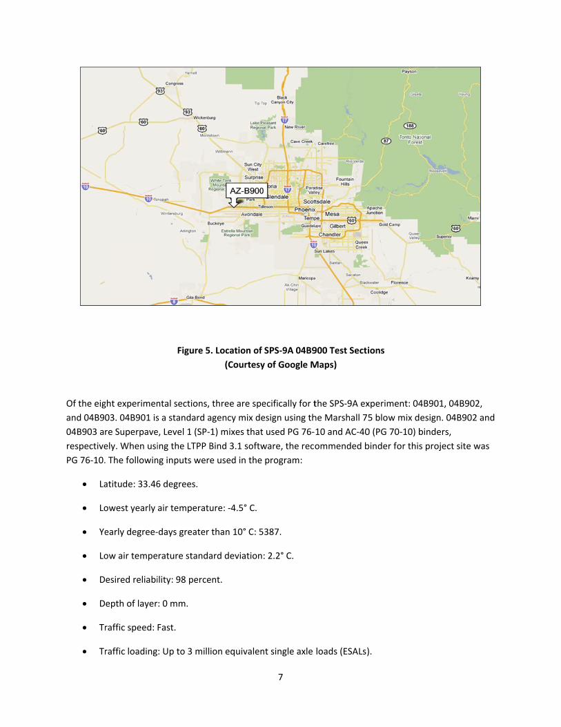
Of the eig

and 04B9

04B903 a

respective

PG 76‐10.

La

Lo

Ye

Lo

D

D

Tr

Tr

ght experimen

03. 04B901 is

re Superpave

ely. When usi

. The followin

atitude: 33.46

owest yearly

early degree‐

ow air tempe

esired reliabi

epth of layer

raffic speed:

raffic loading

Figure 5

ntal sections,

s a standard a

e, Level 1 (SP‐

ing the LTPP B

ng inputs wer

6 degrees.

air temperatu

‐days greater

rature standa

ility: 98 perce

: 0 mm.

Fast.

: Up to 3 mill

5. Location of

(Courtesy

three are spe

agency mix de

1) mixes that

Bind 3.1 softw

e used in the

ure: ‐4.5° C.

than 10° C: 5

ard deviation

ent.

ion equivalen

7

SPS‐9A 04B9

y of Google M

ecifically for t

esign using th

t used PG 76‐

ware, the reco

program:

5387.

: 2.2° C.

nt single axle

900 Test Sect

Maps)

the SPS‐9A ex

he Marshall 7

10 and AC‐40

ommended b

loads (ESALs)

ions

xperiment: 04

5 blow mix d

0 (PG 70‐10) b

binder for this

).

4B901, 04B90

esign. 04B90

binders,

s project site

02,

2 and

was

8

The SPS‐9A experiment also included five supplemental test sections: 04B959, 04B960, 04B961, 04B964,

and 041007/04B962. Sections 04B959, 04B960, and 04B961 were stone mastic asphalt (SMA)

pavements. Section 04B959 was an SMA polymer with an asphalt concrete friction course (ACFC);

04B960 was an SMA polymer pavement; and 04B961 was an SMA cellulose pavement. Section 04B964

was an asphalt rubber asphalt concrete (ARAC) pavement. All mixtures included Type II portland cement

concrete (PCC) as an admixture. Although eight experimental sections were constructed, time and

budget constraints did not allow for detailed information to be recorded on the supplemental sections.

The aggregate properties of Superpave sections 04B902 and 04B903 follow:

Bulk specific gravity of aggregate: 2.672.

Bulk specific gravity of admixture: 3.140.

Bulk specific gravity of the total gradation: 2.677.

Effective specific gravity of the total gradation: 2.712.

Table 2 provides the design mix properties and Table 3 provides the construction mix properties for the

SPS‐9A test sections.

9

Table 2. SPS‐9A Mix Properties (As Designed)

04B901 04B902 04B903 04B960 04B961 All Sections

Layer Agency mix

SP‐1 (PG 76‐10)

SP‐1 (PG 70‐10)

SMA polymer

SMA cellulose

Standard AC below experi‐mental layer

Mix type Marshall Superpave Superpave N/A N/A N/A

Maximum specific gravity

N/A 2.532 2.532 N/A N/A N/A

Bulk specific gravity

2.368 2.425 2.426 N/A N/A N/A

Asphalt content (%) 3.8 4.3 4.3 5.2 5.3 3.4

Air voids (%) 6 4.2 4.2 N/A N/A N/A

Mineral aggregate air voids (%)

N/A 13.3 13.3 N/A N/A N/A

Effective asphalt content (%)

N/A 3.8 3.8 N/A N/A N/A

Number of blows 75 N/A N/A N/A N/A N/A

Asphalt grade N/A N/A AC‐40 AC‐40 N/A N/A

PG high temperature (°C)

76 76 70 N/A N/A N/A

PG low temperature (°C)

10 10 10 N/A N/A N/A

Maximum particle size (mm)

N/A 25.4 25.4 N/A N/A N/A

Bulk density (kg/m3)

2368 N/A N/A N/A N/A N/A

Rice density (kg/m3) 2483 N/A N/A N/A N/A N/A

Avg. (MR) at 5° C N/A 15.663 N/A N/A N/A 19.134



N/A: Not available.

10

Table 3. SPS‐9A Mix Properties (As Constructed)

04B901 04B902 04B903 04B961

Layer Standard AC layer

Agency mix

Standard AC layer

SP‐1 (PG 76‐10)

Standard AC layer

Standard AC layer

SMA cellulose

Mix type N/A N/A N/A Superpave N/A N/A N/A

Bulk specific gravity (mean)

N/A N/A 2.449 N/A N/A N/A N/A

Bulk specific gravity (minimum)


Bulk specific gravity (maximum)


Asphalt content (mean)

3.6 3.7 3.4 4.1 3.3 3.6 5.1

Asphalt content (minimum)

3.6 3.65 3.2 4.0 3.2 3.5 5.1

Asphalt content (maximum)

3.6 3.75 3.7 4.1 3.5 3.8 5.1

Air voids (mean) (%)

3.8 6.2 3.1 3.8 2.4 2.9 3.6

Air voids (minimum) (%)

3.7 5.55 2.1 3.0 N/A 2.6 3.4

Air voids (maximum) (%)

3.8 7.15 4.1 5.1 N/A 3.1 3.8

N/A: Not available.

The dynamic modulus (E*) was calculated for Section 041007/04B962. The E* values provided in Table 4

are estimates based on the resilient modulus Artificial Neural Network model developed in 2011 (Kim et

al. 2011).

11

Table 4. Dynamic Modulus (E*) for Test Section 041007/04B962

Layer Temperature

(°C)

Sample Age

(Days)

Frequency

0.1 0.5 1 5 10 25

Existing AC

14 44 3694828 4074048 4216398 4500353 4603928 4725184

40 44 1967348 2497805 2724167 3225375 3425915 3673586

70 44 532003 834205 994522 1430188 1640226 1931954

100 44 115027 196541 247269 414452 511889 667432

130 44 35623 56534 70009 117823 148342 201351

Standard AC

14 135 4330092 4576202 4664152 4832633 4891801 4959504

40 135 2935557 3421560 3611171 3999767 4144552 4315779

70 135 1127095 1602026 1826265 2367267 2600349 2900745

100 135 282964 474572 585666 917717 1092434 1349704

130 135 79880 134431 169391 289834 363395 485354

SP‐3

14 135 4321909 4573729 4664235 4838556 4900125 4970844

40 135 2919646 3404883 3595022 3986572 4133229 4307322

70 135 1126592 1597170 1819156 2355060 2586341 2884986

100 135 283947 476537 587732 918662 1092199 1347284

130 135 78523 133794 169201 290872 364931 487343

SP‐1 (PG 76‐10)

14 58 4359022 4612543 4703856 4880106 4942501 5014285

40 58 2954525 3439803 3630074 4022336 4169478 4344357

70 58 1155592 1629823 1852780 2389785 2621197 2919867

100 58 295975 494355 608223 945083 1120821 1378316

130 58 81971 139875 176830 303140 379601 505439

The gradations for the Superpave and standard agency aggregate are shown in Figure 6. As previously

mentioned, some mixture and other data were not available for all test sections.

By LTPP definitions, the SPS‐9A project site is a dry, no‐freeze environment (Table 5). The temperature

and precipitation information in Table 5 represents 40 years of recorded data collected at nearby

weather stations. The solar radiation and humidity data were summarized from 15 years of weather

station data from the nearby SPS‐2 project.

12

Figure 6. Gradations of Superpave Aggregate and Agency

Standard Aggregate (FHWA 1998)

Table 5. Climatic Information for SPS‐9A

40‐Year Average

40‐Year Maximum

40‐Year Minimum

Annual average daily mean temperature (°F)

72 74 69

Annual average daily maximum temperature (°F)

88 90 85

Annual average daily minimum temperature (°F)

55 60 51

Absolute maximum annual temperature (°F)

116 123 111

Absolute minimum annual temperature (°F)

25 31 17

Number of days per year above 32 °F

176 196 133

Number of days per year below 32 °F

17 43 1

Annual average freezing index (°F‐days)

0 0 0

Annual average precipitation (inches)

7.7 15.2 1.8

Annual average daily mean solar radiation (W/ft2)

22.7 36.8 1.65

Annual average daily maxi‐mum relative humidity (%)

53 64 43

Annual average daily minimum relative humidity (%)

17 22 13

Restricted zone

Control points

13

Table 6 summarizes the total ESALs computed from traffic‐loading information collected at the SPS‐9

site. The ESAL values for 1993 and 1994 are ADOT estimates; no monitoring traffic data were available

for this period.

Table 6. SPS‐9A Traffic‐Loading Summary

Year ESALs

1993 1,400,000*

1994 1,100,000*

1995 1,283,553

1996 1,253,915

1997 1,289,820

1998 1,374,457

1999 954,526

2000 2,786,163

2001 1,702,068

2002 2,581,494

2003 3,062,289

2004 1,446,194

2005 1,229,188

*ADOT traffic estimates. No monitoring data available.

After experiment surfaces were placed in 1995, the following maintenance activities were performed:

Section 04B901 (agency mix, PG 76‐10): No rehabilitation or maintenance conducted.

Section 04B902 (SP‐1, PG 76‐10): Pothole patching in 2003.

Section 04B903 (SP‐1, PG 70‐10): No rehabilitation or maintenance conducted.

Section 04B959 (SMA polymer with ACFC): No rehabilitation or maintenance conducted.

Section 04B960 (SMA polymer): No rehabilitation or maintenance conducted.

Section 04B961 (SMA cellulose): No rehabilitation or maintenance conducted.

Section 04B964 (ARAC): No rehabilitation or maintenance conducted.

Section 041007/04B962 (SP‐3): Pothole patching in 2003.

14

All test sections were placed out of study because of reconstruction in the summer of 2005 except for

Section 041007/04B962, which was placed out of study in 2007.

Three analyses were conducted on the SPS‐9A project to evaluate pavement performance: deflection,

distress, and profile. The following sections address each analysis, including a description of the research

approach along with performance comparisons between test sections, overall trends, a summary of the

results, and key findings.

15

CHAPTER 2. SPS‐9A DEFLECTION ANALYSIS

Falling weight deflectometer (FWD) data provide information about the overall strength (i.e., stiffness)

of the pavement structure and individual layers. At the SPS‐9A site, researchers used this information to

evaluate changes with time or, as in the case of the asphalt‐bound layers, temperature, and they

performed additional analyses to understand how various design features affect structural performance.

ANALYSIS OF DEFLECTION DATA

Using the nondestructive FWD deflection testing data, researchers can identify the structural condition

of the sections over their service life. In this chapter, three levels of analysis are presented. First,

researchers produced the deflection profile plots of maximum deflection (D0), minimum deflection (D7/

D8), and AREA value for all the sections to identify changes in the pavement and subgrade over time.

Next, they backcalculated subgrade resilient modulus (MR), effective pavement modulus (EP), and

effective structural number (SNeff) as outlined in the AASHTO Guide for Design of Pavement Structures

(AASHTO 1993). Finally, they backcalculated AC modulus and MR using industry standard software.

MAXIMUM DEFLECTION, MINIMUM DEFLECTION, AND AREA VALUE

Maximum Deflections

The normalized average maximum deflection (Dmax) (D0, measured at the center of the FWD load plate,

normalized to a load level of 9000 pounds and an AC mix temperature of 68 °F) typically indicates the

total stiffness of the pavement structure (surface and base) and the underlying subgrade. Increases in

the normalized average maximum deflection (or Dmax) observed over time may be due to weakening of

the pavement structure or weakening of the subgrade.

Figure 7 shows Dmax results for each test section from the first round of testing to the last. Except for

Section 041007, the first round of testing for all sections was performed in 1995. When this testing was

performed, the top lift of the AC layer had not been placed, resulting in the relatively high deflections

that were observed throughout the project. The second test was performed in 1997—21 months after

construction. As expected, Dmax reduced significantly compared to the first round of testing.

Minimum

The minim

LTPP can

also norm

readings w

first round

througho

weakest s

m Deflection

mum deflectio

be either sen

malized to stan

were indicativ

d of testing to

ut the test sit

subgrade. Inte

04B901 0

Figure 7

on (Dmin) was

nsor No. 7 or s

ndard 9000 p

ve of the subg

o the last rou

tes. Section 0

erestingly, su

04B902 04B

. Average No

observed in t

sensor No. 8,

pounds, but n

grade charact

nd of testing

4B964 had th

bgrade stren

B903 04B9

16

ormalized Dma

the sensor fa

depending o

o temperatur

teristics. Figu

. In general, s

he strongest s

gth increased

59 04B960

ax by Test Sec

rthest from t

on the configu

re correction

ure 8 shows th

subgrade mod

subgrade and

d with time in

0 04B961

ction

the loading pl

uration used.

factor was a

he Dmin meas

dulus did not

d Section 04B

n Section 041

04B964 04

late, which fo

The Dmin read

pplied. The D

urement from

t change muc

959 had the

007.

41007

or

dings

Dmin

m the

h

AREA Val

The AREA

section. T

6A

Where

ue

A parameter is

The equation f

106 DD

A = AREA

0D = surfa

1D = surfa

2D = surf

3D = surfa

04B901

Figure 8

s commonly u

for the AREA

32 / DDD

A value

ace deflection

ace deflection

face deflectio

ace deflection

04B902 04

. Average No

used as a mea

value is:

0D

n at center of

n at 12 inches

on at 24 inche

n at 36 inches

4B903 04B9

17

ormalized Dmi

ans of quantif

f test load

s

es

s

959 04B96

in by Test Sec

fying the rela

0 04B961

ction

ative stiffness

04B964 04

s of a paveme

(Eq. 1

41007

ent

1)

18

The AREA value is the normalized area of a slice taken through any deflection basin between the center

of the loaded area and 36 inches. This area is said to be normalized because it is divided by the

maximum deflection, D0. The maximum value of the AREA parameter is 36 inches, which would result

from testing an extremely rigid section of pavement, and it occurs when all four deflections are equal.

The minimum AREA is 11.02 inches, which would result from deflection measurements on a one‐layer

system of homogeneous material. This would imply that the pavement structure is of the same stiffness

as the underlying soil. The state of Washington suggested that general trends of pavement condition can

be concluded from the combination of AREA value and maximum deflection (Table 7) (Mahoney 1995).

Table 7. General Trends of D0 and Area Values (Mahoney 1995)

FWD‐Based Parameter Generalized Conclusions

AREA Dmax

Low Low Weak structure, strong subgrade

Low High Weak structure, weak subgrade

High Low Strong structure, strong subgrade

High High Strong structure, weak subgrade

Figure 9 shows the average AREA value of the SPS‐9A test sections from the first round of testing to the

last round of testing. As shown in the figure, a significant increase in AREA value between first and

second round of testing was observed, which coincides with the Dmax observation.

BACKCALC

The AASH

the effect

data. The

the subgr

and can b

RM

Where

CULATION PR

HTO Guide for

tive modulus

deflections, w

ade‐pavemen

be used to com

rD

P

21

RM = bac

= Poiss

P = applie

r = distan

RD = pav

04B901

Fig

ROCEDURE

r Design of Pa

of all paveme

which are me

nt interface, a

mpute MR. Th

RD

P

ckcalculated s

on’s ratio (

ed load (lbf)

nce from cent

ement surfac

04B902 04

gure 9. AREA

avement Struc

ent layers abo

easured at a d

are considere

he backcalcula

subgrade resi

= 0.5 was as

ter of load pla

ce deflection

4B903 04B

19

A Values by Te

ctures (1993)

ove the subgr

distance at le

ed to reflect t

ated MR can b

lient modulus

ssumed in the

ate to RD (in

at distance r

959 04B96

est Section

outlined a pr

rade, and SNe

ast 0.7 times

he deformati

be calculated

s

e analysis)

nches)

r from the cen

60 04B961

rocedure for

eff using meas

the radius of

ion of the sub

d as:

nter of the lo

04B964 04

calculating M

sured deflecti

f the stress bu

bgrade layer o

(Eq. 2

oad plate (inch

41007

MR,

ion

ulb at

only

2)

hes)

20

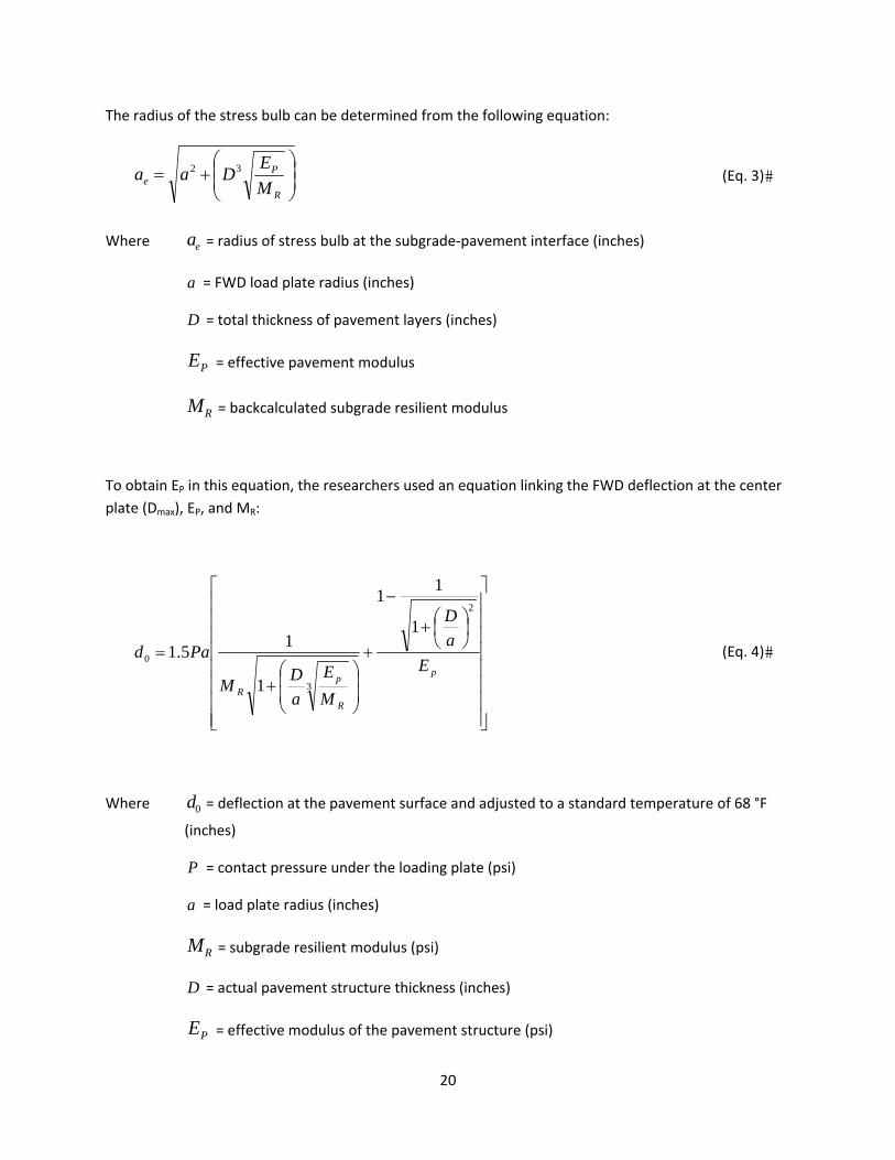
The radius of the stress bulb can be determined from the following equation:

R

Pe M

EDaa 32

(Eq. 3)�

Where ea = radius of stress bulb at the subgrade‐pavement interface (inches)

a = FWD load plate radius (inches)

D = total thickness of pavement layers (inches)

PE = effective pavement modulus

RM = backcalculated subgrade resilient modulus

To obtain EP in this equation, the researchers used an equation linking the FWD deflection at the center

plate (Dmax), EP, and MR:

p

R

pR

E

a

D

M

E

a

DM

Pad

2

3

0

1

11

1

15.1 (Eq. 4)�

Where 0d = deflection at the pavement surface and adjusted to a standard temperature of 68 °F

(inches)

P = contact pressure under the loading plate (psi)

a = load plate radius (inches)

RM = subgrade resilient modulus (psi)

D = actual pavement structure thickness (inches)

PE = effective modulus of the pavement structure (psi)

21

Once EP was determined, SNeff could be calculated:

33.00045.0 peff EDSN � (Eq. 5)�

Where effSN effective structural number

D = total thickness of pavement structure above the subgrade (inches)

PE = effective modulus of the pavement structure above the subgrade (psi)

To accommodate the large quantity of data, the researchers developed a spreadsheet to calculate MR,

EP, and SNeff for each test section. Table 8 presents the statistics of these structural parameters. For

most of the sections, MR remained fairly constant over the monitoring period. The only exception was

observed in Section 041007, where the backcalculated MR jumped from 33 ksi in 1994 to 69 ksi in 1995

and decreased to 33 ksi in 1997. This fluctuation could be due to the construction on the section in

1995. In terms of pavement structure, all test sections showed a similar trend in that EP and SNeff

remained fairly constant in the 1997, 1999, and 2002 testing. However, researchers observed a

decreased EP and SNeff in the last round of testing.

22

Table 8. Structural Parameter Statistics for SPS‐9A

Section Date MR (psi) Ep (psi)

SNeff Average Maximum Minimum

COV (%)

Average Maximum Minimum COV (%)

04B901 1995 28,949 40,648 17,693 19.4 136,723 183,080 98,503 15.0 3.98

04B901 1997 30,949 39,980 21,703 16.4 265,736 366,474 214,224 14.9 5.86

04B901 1999 32,871 41,180 23,327 15.7 274,896 397,821 169,551 19.2 5.87

04B901 2002 37,831 63,421 25,439 27.7 306,204 460,182 156,372 29.2 5.81

04B901 2005 28,529 37,779 19,614 16.3 183,396 311,676 74,500 33.9 4.78

04B902 1995 29,358 32,949 25,105 6.2 134,326 186,140 90,208 17.9 4.00

04B902 1997 32,687 34,782 30,628 4.2 295,456 364,630 240,600 11.5 6.22

04B902 1999 33,542 35,486 30,959 4.5 315,002 393,299 251,270 12.1 6.37

04B902 2002 35,680 43,918 28,849 12.7 332,304 477,059 237,039 20.8 6.24

04B902 2005 29,868 37,235 23,749 12.6 250,433 336,611 182,012 18.1 5.75

04B903 1995 26,580 28,533 24,874 4.1 155,837 230,668 105,480 18.3 4.19

04B903 1997 32,357 41,607 28,577 12.8 286,703 381,018 210,870 13.2 6.33

04B903 1999 31,638 35,479 28,464 5.8 301,070 390,280 234,847 12.6 6.43

04B903 2002 43,805 92,041 29,890 50.4 383,312 631,204 196,096 29.9 6.52

04B903 2005 35,165 53,471 24,310 26.9 279,985 384,813 161,391 23.9 5.91

04B959 1995 19,017 21,774 17,176 6.3 123,133 217,788 68,275 30.5 3.53

04B959 1997 25,928 29,983 21,428 9.2 326,017 462,314 208,958 19.5 6.07

04B959 1999 27,160 31,151 23,189 8.2 315,924 421,827 45,251 24.9 6.10

04B959 2002 25,788 29,404 22,016 8.5 381,757 546,338 246,210 20.6 6.24

04B959 2005 23,765 27,492 20,718 9.0 311,894 436,190 191,329 20.2 5.96

04B960 1995 23,862 25,904 21,126 4.8 171,883 282,444 100,725 24.9 4.03

04B960 1997 30,122 35,505 27,881 6.3 352,891 494,825 279,765 14.8 6.32

04B960 1999 31,379 36,306 29,211 5.2 353,936 498,019 45,357 23.2 6.41

04B960 2002 30,024 33,951 27,723 4.6 413,589 590,113 323,200 15.7 6.61

04B960 2005 29,167 34,731 25,585 7.0 356,083 508,556 248,675 18.0 6.26

04B961 1995 28,151 30,832 24,254 5.5 158,711 236,806 99,114 24.3 3.96

04B961 1997 33,420 36,819 30,685 5.1 372,434 460,651 276,907 13.0 6.44

04B961 1999 34,192 37,360 30,934 4.8 387,084 482,755 287,473 13.6 6.52

04B961 2002 33,709 36,783 31,509 4.7 422,313 528,367 316,203 14.9 6.60

04B961 2005 32,191 38,099 28,905 8.1 374,253 454,893 290,402 13.0 6.40

04B964 1995 38,767 47,576 28,941 14.4 184,452 323,261 108,978 29.0 4.10

04B964 1997 41,652 49,051 30,434 11.4 325,854 425,091 219,385 16.7 6.03

04B964 1999 43,940 52,980 32,478 12.3 319,282 424,569 215,871 18.1 5.99

04B964 2002 46,528 59,964 33,516 14.4 363,137 499,699 251,992 19.8 6.25

04B964 2005 41,183 49,657 29,079 13.7 347,947 455,412 197,200 17.9 6.22

041007 1989 49,092 65,536 36,758 14.4 133,433 194,227 67,490 28.5 3.48

041007 1991 38,798 48,721 30,569 10.0 164,005 263,434 78,824 30.5 3.79

041007 1994 33,301 40,727 26,524 9.9 186,302 289,728 81,070 34.9 3.86

041007 1995 69,973 86,868 55,787 11.9 116,089 178,055 77,353 25.3 4.30

041007 1997 33,205 36,522 27,632 6.1 338,247 461,604 184,745 20.3 6.20

041007 1999 34,584 38,738 28,995 6.1 399,774 529,702 204,192 20.2 6.64

041007 2002 35,338 56,764 26,784 16.6 353,617 537,917 149,727 28.5 5.93

041007 2005 31,516 61,815 24,346 18.5 239,315 461,379 94,113 34.2 5.26

23

BACKCALCULATION USING EVERCALC SOFTWARE

The FWD data were also processed through the backcalculation software Evercalc developed by

Washington State Department of Transportation. One set of FWD data at each station was selected for

backcalculation using the representative thickness of each test section obtained from the LTPP database

to determine MR of each layer. Table 9 shows the seed value and modulus range used for

backcalculation. The pavement structure was first assumed as a four‐layer system for analysis: AC,

aggregate base (AB), subgrade, and bedrock. However, after running several initial analyses, the

researchers found that the base layer was not producing reasonable moduli values. Consequently,

instead of calculating each individual layer moduli, the base layer was combined into the subgrade layer

for consideration, and the backcalculation analysis was repeated. The results of this approach produced

more reasonable moduli values.

Table 9. Backcalculation Seed Value and Modulus Range

Layer Description Seed Modulus

(ksi) Poisson’s Ratio

Minimum Modulus (ksi)

Maximum Modulus (ksi)

AC 400 0.35 100 2100

AB 25 0.3 10 150

Subgrade 15 0.4 5 50

Table 10 provides the statistics of backcalculated moduli for the test sections. A similar pavement

response was observed on the three LTPP test sections (04B901, 04B902, and 04B903). A rapid

increment of the AC moduli was observed in the second round of testing (1997). The AC moduli dropped

significantly in 2002. In general, Sections 04B902 and 04B903 (SP‐1) showed a higher AC moduli value

compared to Section 04B901 (agency standard mix). No significant difference was found between

Section 04B902 (PG 76‐10) and Section 04B903 (PG 70‐10). All three SMA sections (04B959, 04B960, and

04B961) showed superior AC moduli among the eight test sections. Section 04B964 (ARAC) and Section

041007 (SP‐3) showed the lowest AC moduli values.

24

Table 10. Backcalculation Moduli Statistics for SPS‐9A Test Sections

Section Date Backcalculated AC Modulus (ksi)

Backcalculated Subgrade Modulus

(ksi)

Root‐Mean Square Error

(%)

04B901 1995 389.7 25.7 6.07

04B901 1997 693.5 33.5 5

04B901 1999 729.9 35.8 3.72

04B901 2002 340.8 39.4 8.48

04B901 2005 321.7 29.1 3.12

04B902 1995 320.3 23.7 8.2

04B902 1997 793.8 36.8 5.78

04B902 1999 831.8 36.8 5.58

04B902 2002 428.1 38.5 9.9

04B902 2005 468.8 31.1 6.62

04B903 1995 487.8 22.5 4.93

04B903 1997 774 34.9 5.18

04B903 1999 806.4 32.8 4.99

04B903 2002 554.5 42.5 8.17

04B903 2005 554.2 35.4 6.23

04B959 1995 509.4 15.9 2.63

04B959 1997 1257.7 25.1 1.34

04B959 1999 1469.8 27.5 1.93

04B959 2002 833.1 24.2 1.78

04B959 2005 1112.4 22.5 1.77

04B960 1995 303.5 19.4 8.09

04B960 1997 1730 32.5 3.33

04B960 1999 1514.6 33.5 3.8

04B960 2002 723 30.5 5.14

04B960 2005 1309.4 29.8 2.85

04B961 1995 505.4 24 2.23

04B961 1997 1593.7 35.9 2.52

04B961 1999 1563.6 35.5 2.28

04B961 2002 1343.8 36.3 3.06

04B961 2005 1273.4 34.9 2.48

04B964 1995 448.8 31.1 18.87

04B964 1997 703.5 48.2 11.27

04B964 1999 590 48.3 12.47

04B964 2002 353.5 50 18.84

04B964 2005 626.3 45.5 10.25

041007 1989 373.8 30.1 10.1

041007 1991 304.1 29.4 3.66

041007 1994 412.2 24.6 2.17

041007 1995 244.5 24.2 7.18

041007 1997 906.2 32.9 2.71

041007 1999 845.9 34.2 3.43

041007 2002 457.7 34.1 4.39

041007 2005 409.8 30.1 2.17

In genera

AC modul

moduli va

pavement

Figure 11

backcalcu

modulus u

procedure

during the

highest co

lowest CO

l, backcalcula

lus increased

alue is probab

t strength.

shows the ba

ulated subgrad

using the Am

e except Sect

e test period.

oefficient of v

OV was 14 pe

04B9

ated AC modu

with time, w

bly due to the

ackcalculated

de modulus w

erican Associ

ion 041007. I

The average

variation (COV

rcent in Secti

Figure 10.

901 04B902

ulus decrease

which could be

e appearance

d subgrade mo

within each se

iation of State

In general, un

backcalculat

V) of the subg

on 041007.

Backcalculat

2 04B903

25

ed as the pave

e due to aging

of distress an

odulus values

ection is simil

e Highway an

niform subgra

ted subgrade

grade modulu

ted AC Modu

04B959 04

ement aged (

g of the aspha

nd the resulti

s. The variatio

lar to the pre

nd Transporta

ade modulus

modulus of a

us was 21 per

ulus by Test S

4B960 04B9

Figure 10). In

alt binder. Th

ing weakenin

on in the Eve

evious backca

ation Officials

was observed

all sections is

rcent in Sectio

ection

961 04B964

n some cases

he decrease in

g in overall

rcalc

lculated subg

s (AASHTO)

d at the test s

32 ksi. The

on 04B903; th

4 041007

the

n AC

grade

site

he

KEY FIND

The deflec

conducted

testing wa

testing. Th

mainly du

The MR, E

procedure

Th

d

la

d

A

ea

INGS FROM T

ction at the c

d in 1995 and

as completed

he researche

ue to the wea

P, and SNeff re

e follow:

he average EP

ecreased in t

ayer. A decrea

istresses deve

fter the 1995

ach section o

04B9

Figure

THE SPS‐9A D

center plate s

d 1997 as a re

d. All of the se

rs observed a

kening in the

esults after us

P showed an i

he last round

ase of EP was

eloped.

5 construction

over the moni

901 04B902

e 11. Backcal

DEFLECTION A

hows an impr

esult of addin

ections remai

a decline in pa

e AC layer, sin

sing the AASH

increasing tre

d of testing. T

observed in t

n, the average

toring period

2 04B903

26

culated MR b

ANALYSIS

rovement in p

g the structu

ned structura

avement stru

nce the subgra

HTO Guide for

end in the sec

hese results c

the last round

e backcalcula

d.

04B959 04

by Test Sectio

pavement str

ral layer in 19

ally sound du

ucture in the l

ade didn’t ch

r Design of Pa

cond, third, a

can be explai

d of testing b

ted SNeff did

4B960 04B9

on

rength betwe

995 after the

ring the 1997

last round of

ange significa

avement Stru

nd fourth rou

ned by age ha

ecause signif

not change s

961 04B964

een testing

first round o

7, 1999, and 2

testing in 200

antly over tim

uctures (1993)

und of testing

ardening of t

ficant paveme

ignificantly w

4 041007

f

2002

05,

me.

)

g and

he AC

ent

within

27

The results of MR and the AC moduli after using the industrial standard backcalculation software

Evercalc are summarized below:

After construction in 1995, little variation in the AC moduli was observed in most sections. The

first significant drop was observed in 2002 in all sections, however, the AC moduli bounced back

in the 2005 testing. A similar trend was observed among the three core LTPP test sections. The

Superpave mix design sections showed higher AC moduli values compared to the agency

standard mix section. No significant difference was found between the PG 76‐10 and PG 70‐10

sections. The three SMA sections showed the highest AC moduli value among all test sections.

The trend of the Evercalc backcalculated subgrade moduli was similar to the trend observed in

the subgrade moduli using the AASHTO procedure. In general, uniform subgrade modulus was

observed at the test site during the test period. The average backcalculated subgrade modulus

of all sections was 32 ksi. The COV of subgrade modulus within each test section ranged from

14 percent to 21 percent.

29

CHAPTER 3. SPS‐9A DISTRESS ANALYSIS

This chapter includes analyses and results from evaluating distress data collected from the SPS‐9A site

using LTPP manual survey techniques (Miller and Bellinger 2003). Surface distress provides powerful

information about the nature and extent of pavement deterioration, which can be used to quantify

performance trends as well as to investigate how design features affect service life.

All of the flexible SPS‐9A test sections were constructed consecutively and exposed to the same traffic‐

loading, climate, and subgrade conditions, allowing for direct comparisons between layer configurations

and design features without the confounding effects introduced by different in situ conditions.

AC DISTRESS TYPES

Surface deterioration is composed of multiple distress types. The raw distress data for each section are

not included in this report but are available for download from LTPP Products Online

(http://www.infopave.com/Data/StandardDataRelease/). Distress type definitions follow (Huang 1993):

Fatigue cracking: A series of interconnecting cracks caused by repeated traffic loading. Cracking

initiates at the bottom of the asphalt layer where tensile stress is the highest under the wheel

load. With repeated loading, the cracks propagate to the surface.

Longitudinal wheelpath (WP) cracking: Cracking parallel to the centerline occurring in the WP.

This cracking can be the early stages of fatigue cracking or can initiate from construction‐related

issues such as paving seams and segregation of the mix during paving. In the latter case,

cracking is typically very straight (no meandering).

Longitudinal non‐wheelpath (NWP) cracking: Cracking parallel to the centerline occurring

outside the WP. This cracking is not load‐related and can initiate from paving seams or where

segregation issues occurred during paving. Cracking can also be caused by tensile forces

experienced during temperature changes. Pavements with oxidized or hardened asphalt are

more prone to this type of cracking.

Transverse cracking: Cracking that is predominantly perpendicular to the pavement centerline.

Cracking starts from tensile forces experienced during temperature changes. Pavements with

oxidized or hardened asphalt are more prone to this type of cracking.

Block cracking: Cracking that forms a block pattern and divides the surface into approximately

rectangular pieces. Cracking initiates from tensile forces experienced during temperature

changes. This distress type indicates that the AC has significantly oxidized or hardened.

Raveling: Wearing away of the surface caused by dislodging of aggregate particles and loss of

asphalt binder. Raveling is caused by moisture stripping and asphalt hardening.

30

Bleeding: Excessive bituminous binder on the surface that can lead to loss of surface texture or a

shiny, glass‐like, reflective surface. Bleeding is a result of high asphalt content or low air void

content in the mix.

Rutting: A surface depression in the WPs. Rutting can result from consolidation or lateral

movement of material due to traffic loads. It can also signify plastic movement of the asphalt

mix because of inadequate compaction, excessive asphalt, or a binder that is too soft given the

climatic conditions.

These distress types can be grouped into two general categories based on cause of failure mechanism:

structural or environmental factors. Table 11 summarizes the flexible pavement distress types and their

associated failure mechanisms.

Table 11. Flexible Pavement Distress Types and Failure Mechanisms

Distress Type Failure Mechanism

Traffic/Load Related

Climate/Materials Related

Fatigue cracking X

Longitudinal WP cracking X

Longitudinal NWP cracking X

Transverse cracking X

Block cracking X

Raveling X

Bleeding X

Rutting X X

RESEARCH APPROACH

Investigators began this analysis with a cursory review of all distress data collected at each test section

to identify suspect or inconsistent information. Team members used photos and distress maps to verify

quantities reported in the database. Because of the subjective nature of the data collection technique

(raters must select distress type and severity based on a set of rules), variation is expected in distress

data. The SPS‐9A data set was well within the acceptable range of variability.

Distress data are reported at three severity levels: low, moderate, and high. Inconsistencies between

severity levels within a distress type create one of the largest sources of variability in distress data (Rada

et al. 1999). In addition, conducting analyses on three separate severity levels for each distress type

becomes increasingly complex with results that are difficult to interpret. To reduce variability and to

31

consolidate the information for analyses, the researchers summed the quantities from the three severity

levels into one composite value.

As shown in Table 11, pavement deterioration (when not directly attributable to mix problems or

construction deficiencies) can be attributed to structural or environmental factors. Structural factors are

the result of traffic loading relative to the structural capacity of the pavement section. Environmental

factors represent the influence of climate on pavement deterioration. Therefore, structural and

environmental indices were developed to focus the analyses on overall structural and environmental

damage, which are more consistent and provide a better avenue for comparison, rather than on

individual types of distress, which vary from section to section and year to year.

The structural damage index consists of those distresses generally manifesting from the portion of the

pavement that experiences loading (i.e., WPs). Therefore, the structural damage index was presented as

the percentage of WP damage and included fatigue and longitudinal WP cracking. To normalize fatigue

and longitudinal cracking, the structural damage index took the form of the following expression:

swp

lwp

LW

CftFS

2

1 � (Eq. 6)

Where S = structural damage index

F = area of fatigue (ft2)

lwpC = length of longitudinal WP cracking (ft)

wpW = width of WP = 3.28 (ft)

sL = length of test section (ft)

The environmental damage index is a composite of distresses that generally result from climatic effects.

The entire pavement surface is subject to environmental distress; therefore, the environmental damage

index was characterized as the percentage of total pavement area damaged. Typically, transverse

cracking, longitudinal cracking (outside of the WPs), and block cracking are specific to environmental

damage. To normalize the environmental distress for the total area, the environmental damage index

was expressed as:

s

t

s

nwp

tot L

C

L

C

A

BE � (Eq. 7)

32

Where E = environmental damage index

B = area of block cracking (ft2)

nwpC = length of NWP cracking (ft)

tC = length of transverse cracking (ft)

totA = total area of test section (ft2)

sL = length of test section (ft)

Although the structural and environmental distress factors clearly affected the SPS‐9A project’s

structural and functional service life, rutting, patching, and other surface defects (such as potholes,

bleeding, and raveling) also affected performance. Rutting data reported in this study were generated

using a 6 ft straightedge reference (Simpson 2001).

Replicate data were not collected for the SPS‐9A project. Therefore, standard statistical comparisons

(i.e., t tests) to determine the significance of findings could not be conducted. Instead, the evaluation

consisted of graphical comparisons between test sections from data collected at the same points in

time.

OVERALL PERFORMANCE TREND OBSERVATIONS

While gathering pavement distress data, researchers became aware of a few significant trends affecting

the overall pavement performance of the project. These observations were clearly driving issues for this

project and were intrinsically important pieces of the distress performance.

Before receiving the experimental AC overlays, each section received the same rehabilitation treatment

and existing AC was milled. Manual distress surveys were performed on each section after milling, but

before the experimental layers were added. These surveys showed similar conditions throughout all the

sections.

No global preventive maintenance or rehabilitation was performed on any of the test sections. Sections

04B961 and 04B964 exhibited raveling in the 2005 and 2002 surveys, respectively. Sections 04B902 and

041007 exhibited significant pumping; Sections 04B903 and 04B959 experienced minimal pumping.

Figure 12 shows the structural damage trends for each section. The performance trends are relatively

consistent and within the expected range of variation. All sections (except 04B959 and 04B961) showed

a rapid accumulation of structurally related distresses approximately 10 years after construction.

33

The Marshall mix (Section 04B901) contained a smaller percentage of asphalt binder than the Superpave

mixes (Sections 04B902 and 04B903). Higher asphalt binder contents typically produce better resistance

to fatigue cracking; however, all three sections accumulated similar amounts of fatigue cracking.

Compared to the rest of the SPS‐9A project, Section 04B959 (SMA polymer with ACFC) and Section

04B961 (SMA cellulose) exhibited significantly smaller amounts of structural damage accumulation.

Figure 12. Structural Damage Trends for SPS‐9A Test Sections

Figure 13 shows the overall environmental damage trends for each section. The performance trends are

relatively consistent and within the expected range of variation.

Manual Survey Distress Data

0%

20%

40%

60%

80%

100%

120%

140%

160%

Jan-

94

Jan-

95

Jan-

96

Jan-

97

Jan-

98

Jan-

99

Jan-

00

Jan-

01

Jan-

02

Jan-

03

Jan-

04

Jan-

05

Jan-

06

Date

Str

uct

ura

l D

amag

e In

dex

04B901 04B902

04B903 04B959

04B960 04B961

04B964 041007/B962

34

Figure 13. Environmental Damage Trends for SPS‐9A Test Sections

Performance Comparisons

In‐depth analyses and comparisons were conducted for all of the SPS‐9A test sections. Figure 14

summarizes the structural damage index and pavement structure for each section; Figure 15

summarizes the environmental damage index and pavement structure. Both damage indices reported

are based on the data collected in January 2005 (just before going out of study).

Manual Survey Distress Data

0%

50%

100%

150%

200%

250%

300%

350%

Jan-

94

Jan-

95

Jan-

96

Jan-

97

Jan-

98

Jan-

99

Jan-

00

Jan-

01

Jan-

02

Jan-

03

Jan-

04

Jan-

05

Jan-

06

Date

En

viro

nm

enta

l D

amag

e In

dex

04B901 04B902

04B903 04B959

04B960 04B961

04B964 041007/B962

35

Figure 14. Structural Damage Index and Pavement Structure Summary

2005 Manual Distress Data (B900)

108%

140%

111%

3%

102%

15%

100%106%

0%

20%

40%

60%

80%

100%

120%

140%

160%

B901AS PG 76-10

(19mm)

B902SP-1 PG 76-10

(19mm)

B903SP-1 PG 70-10

(19mm)

B959SMA Polymer

W/ACFC

B960SMA Polymer

B961SMA Cellulose

B964ARAC

1007/B962SP-3

Str

uct

ura

l D

amag

e In

dex

04B901 04B902 04B903 04B959 04B960 04B961 04B964 041007/04B962

36

Figure 15. Environmental Damage Index and Pavement Structure Summary

Figure 16 summarizes the rutting and pavement structure for each section. Significant variation in

rutting performance between the sections did not exist. All sections exhibited less than 7 mm of rutting

after over seven years in service, which is well below the level required to trigger improvements in most

pavement management systems. Therefore, rutting was not the driving factor in the overall condition of

the pavement.

2005 Manual Distress Data (B900)

126%

38%

7%

214%

106%

22%

302%

136%

0%

50%

100%

150%

200%

250%

300%

350%

B901AS PG 76-10

(19mm)

B902SP-1 PG 76-10

(19mm)

B903SP-1 PG 70-10

(19mm)

B959SMA Polymer

W/ACFC

B960SMA Polymer

B961SMA Cellulose

B964ARAC

1007/B962SP-3

En

viro

nm

enta

l D

amag

e In

dex

04B901 04B902 04B903 04B959 04B960 04B961 04B964 041007/04B962

37

Figure 16. Rutting Index and Pavement Structure Summary

Following is a synopsis of the findings and performance of each section, including structural

deterioration, environmental deterioration, rutting, and other unique circumstances.

Section 04B901 (Standard Agency Mix, Marshall 75, PG 76‐10)

This section exhibited average cracking performance, both structurally and environmentally. The

structural damage index was 108 percent. Five of eight test sections experienced similar quantities of

structural damage. The environmental damage index was 126 percent. Three of eight test sections

experienced similar quantities of structural damage. The rate of structural and environmental

deterioration increased from 2002 to 2005.

Section 04B902 (SP‐1, PG 76‐10)

This section exhibited the most structural damage of all the test sections; however it performed very

well against environmental damage. The structural damage index was 140 percent, while most sections

experienced quantities near 100 percent. The environmental damage index was 38 percent—much

2005 Rutting Index (B900)

6.2

5.5

6.0

3.83.6

4.1

4.6

6.4

0

1

2

3

4

5

6

7

B901AS PG 76-10

(19mm)

B902SP-1 PG 76-10

(19mm)

B903SP-1 PG 70-10

(19mm)

B959SMA Polymer

W/ACFC

B960SMA Polymer

B961SMA Cellulose

B964ARAC

1007/B962SP-3

Ru

ttin

g I

nd

ex (

mm

)

04B901 04B902 04B903 04B959 04B960 04B961 04B964 041007/04B962

38

lower than the majority of the test sections, which experienced quantities from 100 percent to

300 percent. Section 04B902 also exhibited the highest amount of pumping among the test sections.

The rate of structural deterioration increased from 2002 to 2005.

Section 04B903 (SP‐1, AC‐40 [PG 70‐10])

Structural deterioration was average in this section, but the environmental deterioration was well below

the average for the SPS‐9A project. In fact, Section 04B903 exhibited the highest resistance to

environmental damage. The rate of structural deterioration increased from 2002 to 2005.

Section 04B959 (SMA Polymer with ACFC)

This section exhibited the highest resistance against structural damage for the SPS‐9A project. After

10 years, the structural damage index was at 3 percent, while most sections had a structural damage

index over 100 percent. However, this section also exhibited the second largest amount of

environmental damage of the entire SPS‐9A project as a result of NWP longitudinal cracking along the

edge of the lanes throughout the entire section. The rate of environmental deterioration increased from

2002 to 2005.

Section 04B960 (SMA Polymer)

Like Section 04B901, this section exhibited average cracking performance, both structurally and

environmentally. The structural damage index was 102 percent. Five of eight test sections experienced

similar quantities of structural damage. The environmental damage index was 106 percent. Three of

eight test sections experienced similar quantities of structural damage. The rate of structural and

environmental deterioration increased from 2002 to 2005.

Section 04B961 (SMA Cellulose)

This section was the best‐performing pavement in the entire SPS‐9A project. It was significantly better at

resisting structural and environmental damage throughout the duration of its life when compared to the

other test sections. The environmental and structural damage indices were each approximately

20 percent, which was significantly lower than the majority of the other test sections. Sections 04B961

and 04B964 experienced the highest amount of pavement raveling.

Section 041007/04B962 (SP‐3)

Like Sections 04B901 and 04B960, this section exhibited average cracking performance, both structurally

and environmentally. The structural damage index was 106 percent. Five of eight test sections

experienced similar quantities of structural damage. The environmental damage index was 136 percent.

Three of eight test sections experienced similar quantities of structural damage. Like Section 04B902,

this section exhibited a significant amount of pumping. The rate of structural and environmental

deterioration increased from 2002 to 2005.

39

Section 04B964 (ARAC)

This section performed average against structural damage, but accumulated the highest amount of

environmental damage. The structural damage index was 100 percent. Five of eight test sections

experienced similar quantities of structural damage. However, the environmental damage index was

302 percent, which was significantly higher than all the other test sections. Sections 04B964 and 04B961

experienced the highest amount of pavement raveling.

KEY FINDINGS FROM THE SPS‐9A DISTRESS ANALYSIS

The distress data captured at the SPS‐9A project provide valuable insight into pavement performance,

design, management, and construction. Highlights from the SPS‐9A distress analysis follow:

Most every section (except Sections 04B959 and 04B961) showed significant growth in fatigue

and longitudinal cracking 10 years after construction.

Construction quality can play a major role in performance. The construction observations

documented in the LTPP construction report were limited to Sections 04B901, 04B902, and

04B903. However, the report showed that all three sections were free of any construction

issues.

Half the sections (04B901, 04B959, 04B960, and 041007/04B962) had reasonable patterns of

environmental distress growth with a clear increase in magnitude approximately 10 years after

construction. Section 04B964 had little environmental distress growth for seven years but it

rapidly increased after 10 years.

For the SP‐1 mix designs (Sections 04B902 and 04B903), the PG 70‐10 binder (Section 04B903)

performed significantly better structurally and environmentally than the PG 76‐10 binder

(Section 04B902). It also performed significantly better than the standard agency mix at resisting

environmental deterioration.

SMA with cellulose fibers was, by far, the best pavement mix at resisting both structural and




With no replicate sections, there is limited ability to assess potential variability independent of

actual performance.

Three sections (Sections 04B959, 04B902, and 041007/04B962) received patching at some point.

41

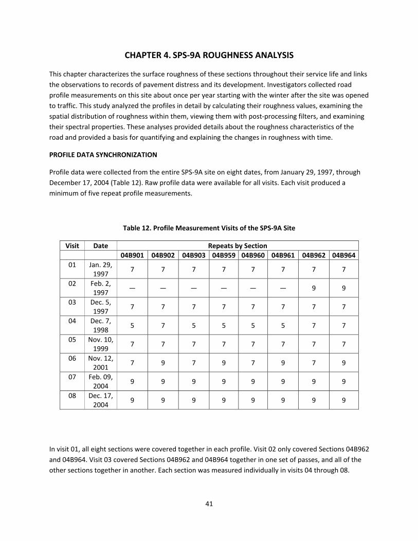
CHAPTER 4. SPS‐9A ROUGHNESS ANALYSIS

This chapter characterizes the surface roughness of these sections throughout their service life and links

the observations to records of pavement distress and its development. Investigators collected road

profile measurements on this site about once per year starting with the winter after the site was opened

to traffic. This study analyzed the profiles in detail by calculating their roughness values, examining the

spatial distribution of roughness within them, viewing them with post‐processing filters, and examining

their spectral properties. These analyses provided details about the roughness characteristics of the

road and provided a basis for quantifying and explaining the changes in roughness with time.

PROFILE DATA SYNCHRONIZATION

Profile data were collected from the entire SPS‐9A site on eight dates, from January 29, 1997, through

December 17, 2004 (Table 12). Raw profile data were available for all visits. Each visit produced a

minimum of five repeat profile measurements.

Table 12. Profile Measurement Visits of the SPS‐9A Site

Visit Date Repeats by Section

04B901 04B902 04B903 04B959 04B960 04B961 04B962 04B964

01 Jan. 29, 1997

7 7 7 7 7 7 7 7

02 Feb. 2, 1997

— — — — — — 9 9

03 Dec. 5, 1997

7 7 7 7 7 7 7 7

04 Dec. 7, 1998

5 7 5 5 5 5 7 7

05 Nov. 10, 1999

7 7 7 7 7 7 7 7

06 Nov. 12, 2001

7 9 7 9 7 9 7 9

07 Feb. 09, 2004

9 9 9 9 9 9 9 9

08 Dec. 17, 2004

9 9 9 9 9 9 9 9

In visit 01, all eight sections were covered together in each profile. Visit 02 only covered Sections 04B962

and 04B964. Visit 03 covered Sections 04B962 and 04B964 together in one set of passes, and all of the

other sections together in another. Each section was measured individually in visits 04 through 08.

42

Researchers used the raw data to synchronize all of the profiles to each other through their entire

history. Three clues were available for this purpose: (1) the site layout from the construction report,

(2) event markers in the raw profiles from the start and end of each section, and (3) automated

searching for the longitudinal offset between repeat measurements.

DATA EXTRACTION

Researchers extracted profiles of individual test sections directly from the raw measurements for two

reasons: First, profiles were collected in visits 01 through 06 at a 0.98‐inch sample interval and in visits

07 and 08 at about a 0.77‐inch sample interval. These data appeared in the database after the

application of an 11.8‐inch moving average and decimation to a sample interval of 5.91 inches. The raw

data contained the more detailed profiles. Second, this study depended on consistency of the profile

starting and ending points with the construction layout and consistency of the section limits with time.

In particular, a previous quality check revealed some profiles were shifted (Evans and Eltahan 2000).

CROSS CORRELATION

Searching for the longitudinal offset between repeat profile measurements that provides the best

agreement between them is a helpful way to refine their synchronization. This can be done by

inspecting filtered profile plots, but it is very time‐consuming. Visual assessment is also somewhat

subjective when two profiles do not agree well, which is often the case when measurements are made

several years apart. In this study, investigators used an automated procedure rather than visual

inspection to find the longitudinal offset between measurements.

In this procedure, which is based on a customized version of cross correlation (Karamihas 2004), a basis

measurement is designated that is considered to have the correct longitudinal positioning. A candidate

profile is then searched for the longitudinal offset that provides the highest cross correlation to the basis

measurement. A high level of cross correlation requires a good match of profile shape, the location of

isolated rough spots, and overall roughness level. Therefore, the correlation level is often only high

when the two measurements are synchronized. When the optimal offset is found, a profile is extracted

from the candidate measurement with the proper overall length and endpoint positions. For the

remainder of this discussion, this procedure will be referred to as automated synchronization.

For this application, investigators performed cross correlation after the International Roughness Index

(IRI) filter was applied to the profiles rather than using the unfiltered profiles, which helped assign the

proper weighting to relevant profile features. In particular, it increased the weighting of short‐

wavelength roughness that may be linked to pavement distress. This enhanced the effectiveness of the

automated synchronization procedure. The long‐wavelength content within the IRI output helped

ensure that the longitudinal positioning was nearly correct, and the short‐wavelength content was able

to leverage profile features at isolated rough spots to fine‐tune the positioning.

43

SYNCHRONIZATION

To extract profiles of individual test sections from the raw measurements, investigators:

1. Established a basis measurement for each section from visit 08. The first repeat measurement

was used for this purpose. All of the sections were 500 ft long.

2. Automatically synchronized the other eight repeats from visit 08 to the basis set.

3. Automatically synchronized the measurements from the previous visit to the current basis set.

4. Designated the previous visit as the current visit.

5. Replaced the basis set with a new set of synchronized measurements from the first repeat of

the current visit.

6. Repeated steps 3 through 5 until visit 01 was complete.

DATA QUALITY SCREENING

Investigators performed data quality screening to select five repeat profile measurements from each

visit of each section. Among the group of available runs, investigators selected the five measurements

that exhibited the best agreement with each other. In this case, agreement between any two profile

measurements was judged by cross‐correlating them after applying the IRI filter (Karamihas 2004). In

this method, the IRI filter is applied to the profiles; then the output signals are compared rather than the

overall index. High correlation by this method requires that the overall roughness as well as the details

of the profile shape that affect the IRI agree. The IRI filter was applied before correlation in this case for

several reasons:

• Direct correlation of unfiltered profiles places a premium on very long‐wavelength content, but

ignores much of the contribution of short‐wavelength content.

• Correlation of IRI filter output emphasizes profile features in (approximate) proportion to their

effect on the overall roughness.

• Correlation of IRI filter output provides a good trade‐off between emphasizing localized rough

features at distressed areas in the pavement and placing too much weight on the very short‐

duration, narrow features (spikes) that are not likely to agree between measurements because

the IRI filter amplifies short‐wavelength content, but attenuates macrotexture, megatexture,

and spikes.

• A relationship has been demonstrated between the cross‐correlation level of IRI filter output

and the expected agreement in overall IRI (Karamihas 2004).

44

Note: This method was performed with a special provision for correcting modest longitudinal distance

measurement errors.

Each comparison between profiles produced a single value that summarized their level of agreement.

When nine repeat profile measurements were available, they produced 36 correlation values. Any

subgroup of five measurements could be summarized by averaging the relevant 10 correlation values.

Researchers selected the subgroup that produced the highest average and excluded the other repeats

from most of the analyses discussed in the remainder of this report. Since the number of available

profiles ranged from six to nine, the number of measurements that were excluded ranged from one to

four. Tables 13 through 20 list the selected repeats for each visit of each section and the composite

correlation level produced by them.

Table 13. Selected Repeats of Section 04B901

Visit Repeat Numbers Composite Correlation

01 1 2 3 5 6 0.901

03 1 3 4 5 7 0.898

04 1 2 3 4 5 0.916

05 2 4 5 6 7 0.912

06 2 3 4 6 7 0.870

07 1 3 5 7 9 0.659

08 2 3 5 7 8 0.722



01 2 3 4 5 7 0.935

03 1 3 4 5 7 0.896

04 1 2 4 5 6 0.931

05 2 3 4 5 6 0.871

06 5 6 7 8 9 0.827

07 3 6 7 8 9 0.639

08 1 5 7 8 9 0.768



01 2 3 5 6 7 0.929

03 1 2 4 6 7 0.914

04 1 2 3 4 5 0.918

05 3 4 5 6 7 0.943

06 1 3 4 6 7 0.894

07 1 3 5 6 7 0.853

08 1 2 3 8 9 0.588

45



01 1 3 4 6 7 0.932

03 1 2 4 5 7 0.923

04 1 2 3 4 5 0.921

05 2 3 4 5 6 0.922

06 2 5 7 8 9 0.944

07 1 3 5 6 7 0.905

08 3 5 6 8 9 0.870



01 1 2 3 5 7 0.925

03 1 2 4 6 7 0.915

04 1 2 3 4 5 0.903

05 1 2 3 4 6 0.924

06 1 2 3 4 7 0.949

07 1 2 3 4 5 0.853

08 5 6 7 8 9 0.864



01 1 2 3 4 7 0.943

03 2 4 5 6 7 0.948

04 1 2 3 4 5 0.915

05 1 2 4 5 7 0.942

06 1 2 3 4 6 0.953

07 2 3 5 6 9 0.901

08 1 6 7 8 9 0.826



01 2 3 4 6 7 0.873

02 2 4 5 7 9 0.910

03 1 2 4 5 7 0.876

04 1 2 5 6 7 0.914

05 1 2 3 4 6 0.901

06 1 2 3 4 6 0.793

07 3 5 6 8 9 0.735

08 1 3 4 6 7 0.651

46



01 1 2 4 5 6 0.914

02 2 5 7 8 9 0.934

03 1 2 5 6 7 0.878

04 1 2 4 5 6 0.888

05 1 2 5 6 7 0.883

06 2 3 6 7 9 0.937

07 1 5 7 8 9 0.833

08 1 2 4 6 9 0.728

The process for selecting five repeat measurements from a larger group is similar to the practice within

LTPP except that it is based on composite agreement in profile rather than the overall index value. The

correlation levels listed in Tables 13 through 20 provide an appraisal of the agreement between profile

measurements for each visit of each section. When two profiles produce a correlation level above 0.82,

their IRI values are expected to agree within 10 percent most (95 percent) of the time. Above this

threshold, the agreement between profiles is usually acceptable for studying the influence of distresses

on profile. When two profiles produce a correlation level above 0.92, they are expected to agree within

5 percent most of the time. Above this threshold, the agreement between profiles is good. Correlation

above 0.92 often depends on consistent lateral tracking of the profiler and may be very difficult to

achieve on highly distressed surfaces. The IRI values provided in this report will be the average of five

observations, which will tighten the tolerance even further.

Overall, most of the groups of measurements in Tables 13 through 20 exhibited good or better

correlation, and most exhibited acceptable correlation. Any group of repeat measurements that

produced a composite correlation level below 0.82 was investigated using filtered plots; these results

follow:

Section 04B901, visit 07 and 08: Narrow downward spikes throughout the profiles significantly

diminished the correlation.

Section 04B902, visit 07: Narrow downward spikes throughout the left side profiles significantly

diminished the correlation. These appeared in the same location in some, but rarely all, repeat

measurements.

Section 04B902, visit 08: Narrow downward spikes in isolated locations within the profiles

significantly diminished the correlation.

Section 04B903, visit 08: Narrow downward spikes in the left side profiles significantly

diminished the correlation. These appeared in the same location in some, but rarely all, repeat

measurements.

47

Section 04B961, visit 08: Correlation was diminished by short‐wavelength “noise” throughout

the section on both the left and right side and several extraneous spikes in the left side profiles.

Section 04B962, visits 06 through 08: Narrow downward spikes that rarely appeared in the same

location in more than two repeat measurements significantly diminished the correlation.

Section 04B964, visits 07 and 08: Correlation was diminished by short‐wavelength “noise”

throughout the section on both the left and right side.

SUMMARY ROUGHNESS VALUES

Figures 17 through 24 show the left and right IRI values for each pavement section over its monitoring

period. For most of the sections, this includes 14 summary IRI values: two per visit over seven visits. The

figures show the IRI values versus time in years. In this case, “years” refers to the number of years

between the measurement date and April 1, 1995. (All of the test sections were constructed in the

second half of March 1995.) Fractions of a year are estimated to the nearest day.

To supplement the plots, the appendix to this report lists the IRI, Half‐car Roughness Index (HRI), and

Ride Number (RN) of each section for each visit. These roughness values are the average of the five

repeat measurements selected in the data quality screening. These are not necessarily the same five

repeat measurements selected for the LTPP database. The appendix also provides the standard

deviation of IRI over the five repeat measurements to help identify erratic roughness values that result

from transverse variations in profile caused by surface distresses.

Figures 17 through 24 provide a snapshot of the roughness history of each pavement section. The

remainder of this chapter characterizes the profile content that made up the roughness and explains the

profile features that contributed to roughness progression.

48

Figure 17. IRI Progression of Section 04B901


0

50

100

150

0 2 4 6 8 10

RightLeft

Years

IRI (in/mi)

Section B901

0

50

100

150

0 2 4 6 8 10

RightLeft

Years

IRI (in/mi)

Section B902

IRI (inches/mile)

IRI (inches/mile)

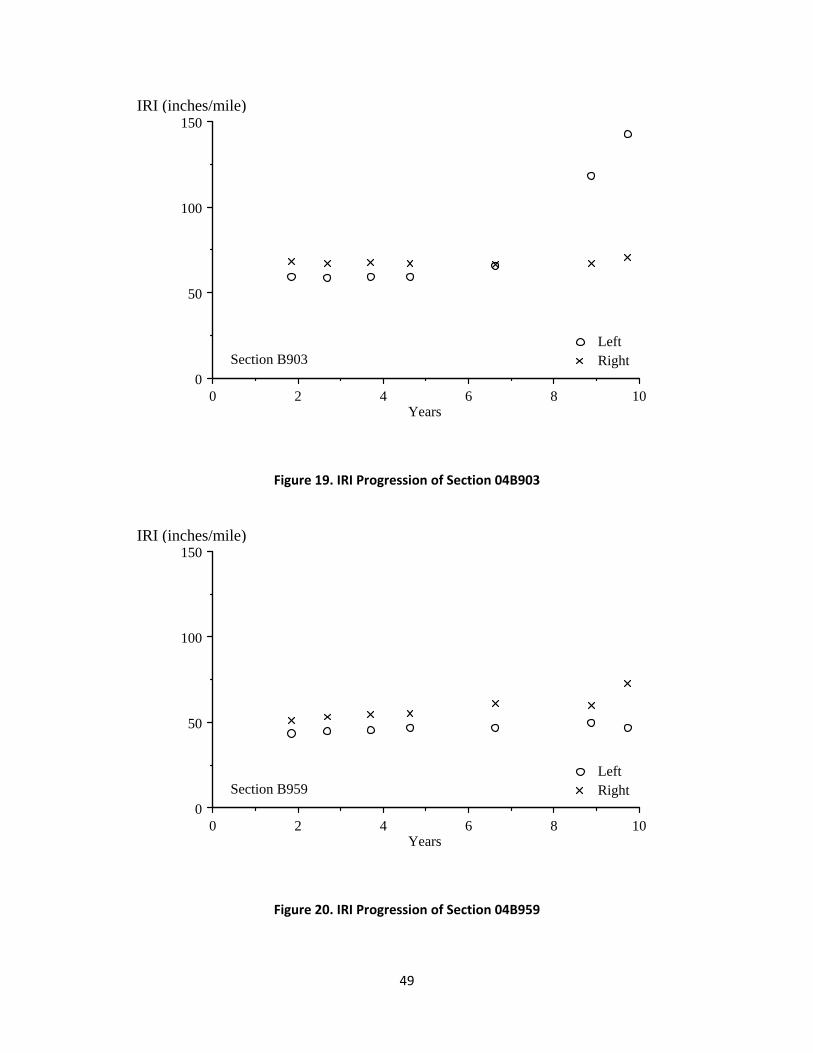
49



0

50

100

150

0 2 4 6 8 10

RightLeft

Years

IRI (in/mi)

Section B903

0

50

100

150

0 2 4 6 8 10

RightLeft

Years

IRI (in/mi)

Section B959

IRI (inches/mile)

IRI (inches/mile)

50



0

50

100

150

0 2 4 6 8 10

RightLeft

Years

IRI (in/mi)

Section B960

0

50

100

150

0 2 4 6 8 10

RightLeft

Years

IRI (in/mi)

Section B961

IRI (inches/mile)

IRI (inches/mile)

51


0

50

100

150

200

250

300

0 2 4 6 8 10

RightLeft

Years

IRI (in/mi)

Section B962

IRI (inches/mile)

52


PROFILE ANALYSIS TOOLS

Investigators used various analytical techniques to study the profile characteristics of each pavement

section and their change with time. These tools help study roughness, roughness distribution, and

roughness progression of each test section, including concentrated roughness that may be linked to

pavement distress. The discussion of each analysis and plotting method is rather brief; Sayers and

Karamihas (1996b) provide more details about these methods.

Roughness Values

Investigators calculated left IRI, right IRI, Mean Roughness Index (MRI), HRI, and RN values. The

appendix provides the average value of each index for each visit of each section. The discussion of

roughness in this analysis emphasizes the left and right IRI. Nevertheless, comparing the progression of

HRI and RN to the MRI provides additional information about the type of roughness that is changing. For

example, a low HRI value relative to MRI indicates roughness that exists on only one side of the lane.

Further, aggressive degradation of RN without a commensurate growth in MRI signifies that the

developing roughness is biased toward short‐wavelength content.

0

50

100

150

0 2 4 6 8 10

RightLeft

Years

IRI (in/mi)

Section B964

IRI (inches/mile)

53

Elevation Profile Plots

A simple way to learn about the type of roughness that exists within a profile is to view the trace.

However, certain key details of the profile are often not as obvious in a raw profile trace as they may be

after the profile is filtered. Three types of filtered plots were inspected for every visit of every section:

Long wavelength: A profile smoothed with a base length of 25 ft and anti‐smoothed with a base

length of 125 ft.

Medium wavelength: A profile smoothed with a base length of 5 ft and anti‐smoothed with a

base length of 25 ft.

Short wavelength: A profile smoothed with a base length of 1 ft and anti‐smoothed with a base

length of 5 ft.

These filters were used to screen the profiles for changes with time and special features of interest. The

terms “long,” “medium,” and “short” are relative, and in this case pertain to the relevant portions of the

waveband that affects the IRI. The long‐wavelength portion of the profile was typically very stable with

time. However, the long‐wavelength profile plots of every section changed somewhat between visit 06

and 07—not by a change in the surface characteristics of the section, but by a change in profiler make

and the associated change in filtering practices.

The medium‐wavelength plots provided a view of the features in a profile that were likely to have a

strong effect on the IRI and may change with time. The short‐wavelength elevation plots also typically

progressed with time, but only affected the IRI through localized roughness or major changes in content

with time. However, the short‐wavelength elevation plots helped identify and track the progression of

narrow dips and other short‐duration features that may have been linked to distress.

In addition to filtered plots, every profile was viewed in its raw form. This helped reveal noteworthy

features that did not necessarily affect the IRI, but helped establish a link between surface distress and

profile properties. Two examples of this were narrow downward spikes in the profiles caused by

cracking and deep, short‐duration dips at potholes.

Roughness Profile

A roughness profile provides a continuous report of road roughness using a given segment length

(Sayers 1990). Instead of summarizing the roughness by providing the IRI for an entire pavement

section, the roughness profile shows how IRI varies with distance along the section by using a sliding

window to display the IRI of every possible segment of given base length along the pavement.

A roughness profile displays the spatial distribution of roughness within a pavement section. As such, it

can be used to distinguish road sections with uniform roughness from sections with roughness levels

54

that change over their length. Further, the roughness profile can pinpoint locations with concentrated

roughness and estimate the contribution of a given road disturbance to the overall IRI.

In this work, roughness profiles were generated and viewed using a base length of 25 ft, that is, every

point in the plot shows the IRI of a 25‐ft segment of road, starting 12.5 ft upstream and ending 12.5 ft

downstream. Any location where a peak occurs in the roughness profile that is greater than or equal to

2.5 times the average IRI for the entire section is considered an area of localized roughness. All areas of

localized roughness are discussed in the detailed observations by identifying them, listing their severity,

and describing the underlying profile features that caused them.

Power Spectral Density Plots

A power spectral density (PSD) plot of an elevation profile shows the distribution of its content within

each waveband. An elevation profile PSD is displayed as mean square elevation versus wave number,

which is the inverse of wavelength. PSD plots were calculated from the slope profile rather than the

elevation profile, which aided in the interpretation of the plots because the content of a slope PSD

typically covers fewer orders of magnitude than an elevation PSD.

A PSD plot is generated by performing a Fourier transform on a profile (or in this case, a slope profile).

The PSD’s value in each waveband is derived from the Fourier coefficients and represents the

contribution to the overall mean square of the profile in that band.

The slope PSD plots provided a very useful breakdown of the content within a profile. In particular, the

plots reveal (1) cases in which significant roughness is concentrated within a given waveband; (2) the

type of content that dominates the profile (e.g., long, medium, or short wavelength); (3) the type of

roughness that increases with time; and (4) the type of roughness that is stable with time.

For this project, the PSDs rarely provided much value beyond what was learned using filtered elevation

plots and roughness profiles. However, any valuable observations that could be made from a PSD plot

are discussed in the following section.

Distress Surveys

Once the analysis and plotting were completed, all of the observations were compared to the manual

distress surveys performed on each section. Manual distress survey results were available for each

section on at least six dates over the monitoring history, starting in February 1995. These were

performed using LTPP protocols by technicians certified to perform distress surveys. The surveys

provided a means of relating profile features to known distresses.

DETAILED OBSERVATIONS

This section reports key observations from the roughness index progression, filtered elevation profile

plots, roughness profiles, PSD plots, and distress surveys. In many cases, similar behavior was noted for

multiple sections. These observations are repeated under the heading of every section where

55

appropriate. However, changes in profile properties with time that were caused by changes in profiler

make or model are summarized at the end of the report.

Section 04B901

Roughness

The IRI of the left side increased steadily from 66 to 90 inches/mi over the monitoring period, with the

exception of a value of 128 inches/mi in visit 07. The IRI of the right side increased from 65 to

103 inches/mi over the monitoring period, but most of the increase occurred in the last two visits. The

HRI was 11 percent to 14 percent below the MRI in visits 01 through 06, and was 19 percent to

21 percent below the MRI in visits 07 and 08.


The left side profiles were very consistent with each other over the first five visits. Visit 06 profiles were

also consistent with previous visits in the medium‐ and long‐wavelength range. However, the agreement

in the short‐wavelength range was not as good because of narrow downward spikes in some locations

within the visit 06 profiles. By visit 07, a very high concentration of narrow downward spikes up to 0.5

inch deep appeared in the left side profiles over the entire length of the section. These sometimes

appeared at the same location in more than one repeat measurement, but rarely appeared in all five. In

visit 08, very few narrow downward spikes appeared in the profiles with the exception of a patch of

spikes about 0.5 inch deep that occurred 5 to 10 ft and 37 to 39 ft from the start of the section.

The right side profiles were consistent with each other over the first six visits. (A minor exception was

repeat 5 from visit 01, which was different from the others in the long‐wavelength range.) Visit 07

profiles were very similar to those of previous visits except they included several narrow downward

spikes that were rarely in the same location in more than one repeat measurement. The spikes

appeared with the highest density in the last 140 ft of the section. Profiles from visit 08 included a much

higher number of downward spikes over the entire section, and they were most prevalent in the first

100 ft of the section.

Two bumps stood out in the right side profiles from all seven visits. The first was about 115 ft from the

start of the section and was 4 ft long and up to 0.15 inch high. The second was about 200 ft from the

start of the section and was about 10 ft long and 0.2 inch high.

Roughness Profiles

The left side roughness profiles were very consistent in visits 01 through 05. No localized roughness

appeared in these visits, although the roughness was not particularly evenly distributed. The roughness

was highest about 125 ft from the start of the section. This is near a series of four bumps up to 5 ft long

and more than 0.1 inch high. The final bump in the series was about 131 ft from the start of the section.

It was 5 ft long and over 0.2 inch high. By visit 08, the peak value of the roughness profiles in this

location was 195 to 215 inches/mi.

56

In visits 06 and 07, the roughness profiles were not consistent with each other because of the hit‐or‐

miss nature of the downward spikes within the elevation profiles.

The right side roughness profiles were fairly consistent with each other in visits 01 through 06. In visits

07 and 08, additional roughness appeared in every repeat measurement, but rarely in the same

locations in any two repeats. Localized roughness appeared in all visits within the last 25 ft of the

section. This area had peak roughness values of over 160 inches/mi in all visits. This roughness was

caused by a series of disturbances about 5 ft long. (It is not clear if these are bumps or dips.) In visit 07

and one repeat measurement from visit 08, the peak roughness was much higher in this location

because a narrow dip up to 1 inch deep appeared 480.5 ft from the start of the section in these profiles.

Distress Surveys

WP cracking was first recorded in January 1999. This covered more than half of the left WP. By April

2002 cracking had covered all of the left WP, and longitudinal cracking covered about half of the right

WP. In January 2005, areas of cracking covered both WPs over the entire length of the section.

Transverse cracking was also recorded on both sides in multiple locations. (Ten feet of longitudinal

distance without at least one transverse crack was rare.) Nothing in the distress surveys explain the

localized roughness on the left side described above or the reduction in roughness on the left side

between visits 07 and 08. The narrow dip 480.5 ft from the start of the section on the right side is in

about the same location as a transverse crack recorded in April 2002 and January 2005.

Section 04B902

Roughness

The IRI of the left side did not follow a clear trend, but increased overall from 58 inches/mi in visit 01 to

79 inches/mi in visit 08. In visit 07, the left side IRI averaged 143 inches/mi, with a standard deviation of

28.1 inches/mi. These values were much higher than in any other visit. The IRI of the right side held

steady between 59 and 63 inches/mi in visits 01 through 06, then increased to 89 inches/mi by visit 08.

The HRI was 14 percent to 22 percent below the MRI.


The right side profiles were consistent in visits 01 through 06, and similar in visit 07. (A minor exception

was repeat 5 from visit 01, which was different from the rest in the long‐wavelength range.) A bump

appears in the profiles of all visits from 195 to 203 ft that is about 0.2 inch high. The profiles from visit

08 include narrow downward spikes throughout the section. These often appear in only one repeat

measurement in a given specific location, but some areas have a higher density of spikes than others.

The left side profiles were consistent in visits 01 through 05. (A minor exception was repeat 5 from visit

01, which was different from the rest in the long‐wavelength range.) A patch of densely spaced narrow

dips, up to 0.3 inch deep, appeared 120 to 145 ft from the start of the section in visit 05. Three new

areas of densely spaced narrow dips appeared in the visit 06 profiles, from 215 to 235 ft, 305 to 330 ft,

and 405 to 435 ft from the start of the section.

57

All visit 07 profiles included narrow downward spikes throughout the entire length of the section. These

spikes were typically 0.4 inch or more deep and were poorly correlated among the five repeat

measurements. Visit 07 profiles also included four bumps about a foot long: (1) about 120 ft from the

start of the section, 0.5 inch high; (2) about 134 ft from the start of the section, 0.35 inch high; (3) about

304 ft from the start of the section, 0.2 inch high, detected in two repeats; and (4) about 307 ft from the

start of the section, 0.3 inch high, detected in four repeats.

Visit 08 profiles included narrow dips in the same areas as visit 06 along with a few narrow downward

spikes in other areas. None of the four bumps listed for visit 07 appeared in the visit 08 profiles. The

patches of narrow dips in visit 08 were much more repeatable, isolated, and in some cases more severe

than in previous visits.

Roughness Profiles

An area of localized roughness appeared in the right side profiles about 197 ft from the start of the

section in all visits. This was caused by the 8‐ft‐long bump described above. A peak also appeared in

visits 01 through 07 of up to 140 inches/mi that is 120 ft from the start of the section. It was caused by a

bump about 0.1 inch high from 113 to 117 ft from the start of the section. The right side roughness

profiles from visit 08 were not very consistent because of the lack of repeatability in the appearance of

the narrow downward spikes.

The roughness profiles from the left side included localized roughness in four of the five repeat

measurements about 135 ft from the start of the section in visit 05. In visit 06, and particularly in repeat

6, the roughness profiles showed a significant increase over those of visit 05 in the areas where the

narrow dips appeared. Visit 07 was much rougher than visit 06 in several areas, again because of the

narrow dips. The roughness was highest in the first 150 ft of the section and in the last 100 ft (in repeat

7 only).

Visit 08 roughness profiles were much more repeatable on the left side than in visits 06 and 07. Areas of

high roughness were centered about 125, 220, 315, and 420 ft from the start of the section.

Distress Surveys

The patch of narrow dips in the left side profiles in visit 05 corresponds to an area of cracking recorded

in the left WP in January 1999. This was the only cracking recorded in that survey. In April 2002, the

distress survey recorded areas of cracking over most of the left WP and longitudinal cracking over much

of the length of the section in the right WP.

Three of the four bumps listed for the left side profiles in visit 07 appear in locations where potholes

were recorded in January 2005. The only pothole that was not in the vicinity of a corresponding bump

was about 235 ft from the start of the section. In January 2005, potholes were detected in the left WP

121, 235, 305, 307, and 312 ft from the start of the section. These were locations where narrow dips

were the most prevalent in visit 08 profiles, and all of these areas corresponded to peaks in the

roughness profiles from visit 08.

58

Section 04B903

Roughness

The IRI of the left side increased from 59 to 66 inches/mi in visits 01 through 06, then increased to

143 inches/mi by visit 08. The IRI of the right side held steady between 67 and 71 inches/mi over the

monitoring period. The HRI was 15 percent to 20 percent below the MRI.


In visit 06, narrow dips began to emerge in the left side profiles. They were up to 0.15 inch deep and

appeared in the same location in more than one profile in some cases. Visit 07 profiles included more

narrow dips on the left side. The dips were up to 0.5 inch deep, and the majority of them did not appear

in the same location in multiple repeat measurements. Visit 08 included a much higher density of

narrow dips. Many of the dips under 0.3 inch deep were not well repeated, but several deeper dips

appeared at the same location in more than one repeat measurement.

Similar dips appeared in the right side profiles from visits 06 through 08, but not nearly as many, and

they were much less severe.

A dip 1 ft long and at least 2.4 inches deep appeared in the left side profiles from visit 07 about 122 ft

from the start of the section. A dip 1 ft long and 2 inches deep appeared in three of the five left side

profiles from visit 08 about 333 ft from the start of the section.

Roughness Profiles

The roughness was very uniform along the section on the left side in visits 03 and 04. In visit 06, the

roughness was somewhat uniform along the section, but not very consistent among the repeat

measurements. Severe localized roughness with a peak value of 540 inches/mi appeared in the location

of the deep dip in visit 07. This feature alone added more than 25 inches/mi to the overall IRI of the left

side. Severe localized roughness with a peak value of 630 to 695 inches/mi appeared about 333 ft from

the start of the section in three of the five repeat measurements from visit 08. This accounted for about

30 inches/mi of additional roughness in those repeat measurements. It also explains the high

(15.4 inches/mi) standard deviation among the left side IRI values.

No localized roughness was found in the right side profiles; they were very consistent with time in

visits 01 through 07.

Distress Surveys

No distress was recorded until April 2002 when longitudinal cracking and large areas of WP cracking

were recorded. In January 2005, both WPs were covered with cracking over the entire length of the

section. Nothing in the distress survey explains the deep dips in visits 07 and 08.

59

Section 04B959

Roughness

The IRI of the left side increased from 41 inches/mi in visit 01 to 47 inches/mi in visit 08 with a peak

value of 50 inches/mi in visit 07. The IRI of the right side increased steadily from 51 to 73 inches/mi. The

HRI was 13 percent to 16 percent below the MRI.


Profiles were very consistent over the monitoring period on the left side. The only feature that stood out

was a dip at the start of the section 0.1‐0.2 inch deep and about 10 ft long. The deepest part of the dip

was only a few feet from the start of the section. Its shape was only fully developed in profiles that

included lead‐in, such as visits 07 and 08.

The right side profiles included narrow dips 188.5 ft from the start of the section in some of the repeat

measurements from visits 04 and 05. But the profiles were fairly consistent in visits 01 through 07. In

visit 08, several narrow dips up to 0.1 inch deep appeared, particularly in the first third of the section.

Roughness Profiles

The roughness of the left side was uniform along the section with the exception of localized roughness

at the very start of the section, which was caused by the long dip described above and roughness that

appeared just ahead of the section start. The localized roughness only appeared in visits 07 and 08

because they included profiles upstream of the section start.

In the early visits, the roughness of the right side was uniform along the section. In later visits, and

particularly in visit 08, most of the increase in roughness occurred in the first third of the section.

Distress Surveys

Nothing in the distress surveys explains the narrow dip in visits 04 and 05. Very little distress was

recorded before January 2005. By January 2005, significant cracking had appeared. Much of the cracking

was found in the first third of the section along the right WP. This included transverse cracks and large

areas of cracking within the WP. Narrow dips appeared in the visit 08 profiles in the position of most of

the transverse cracks.

Section 04B960

Roughness

The IRI of the left side held steady between 45 and 47 inches/mi in visits 01 through 06, then increased

to 54 inches/mi by visit 08. The IRI of the right side only ranged from 45 to 48 inches/mi. The HRI was

13 percent to 18 percent below the MRI.

60


The right side profiles were very consistent with time. Two small disturbances stood out in the medium‐

wavelength (and raw) profiles that were about 190 and 380 ft from the start of the section. The same

features appeared on the left side, but they did not stand out among the roughness from the rest of the

section. The left side profiles were very consistent with time in visits 01 through 06. In visit 07, a sunken

area appeared 441 to 447 ft from the start of the section that included two dips within it, each at least

0.1 inch deep. In visit 08, this entire area was about 0.1 inch below the surrounding pavement, and it

included three dips within it, each at least another 0.2 inch deep.

Roughness Profiles

The right side roughness profiles were very consistent with time. In all visits, the roughness was about

double the average near 190 and 380 ft from the start of the section. The left side roughness profiles

were fairly consistent with time in visits 01 through 06. In visit 07, a peak of about 100 inches/mi

appeared in the roughness profile about 445 to 450 ft from the start of the section. By visit 08, the same

area showed peak roughness of up to 160 inches/mi. This localized roughness was caused by the sunken

area with dips described above and was responsible for the majority of the increase in roughness of the

entire section after visit 06.

Distress Surveys

The distress surveys recorded very little distress before April 2002. Some transverse and longitudinal

cracking was recorded in April 2002. This included longitudinal cracking from 435 to 450 ft from the start

of the section on the left side of the lane and transverse cracking across the left WP about 443 and

447 ft from the start of the section. This corresponds to the sunken area and the dips within it described

above. The distress survey from January 2005 observed cracking over the entire section in both WPs, but

several transverse cracks in the area from 440 to 450 ft were also specifically recorded.

Section 04B961

Roughness

The IRI increased from 52 to 59 inches/mi on the left side, but the progression was not steady. The IRI

only ranged from 56 to 60 inches/mi on the right side. The HRI was 10 percent to 12 percent below the

MRI. This was the lowest difference observed for the SPS‐9A project, and it is an unusually low

difference for a full‐depth asphalt pavement.


Profiles were very consistent over the monitoring period on both sides of the lane. They were unusually

consistent with time in the short‐wavelength range. Very few features stood out. One minor exception:

a series of short (about 0.05 inch), narrow bumps 60 to 100 ft from the section start on both sides.

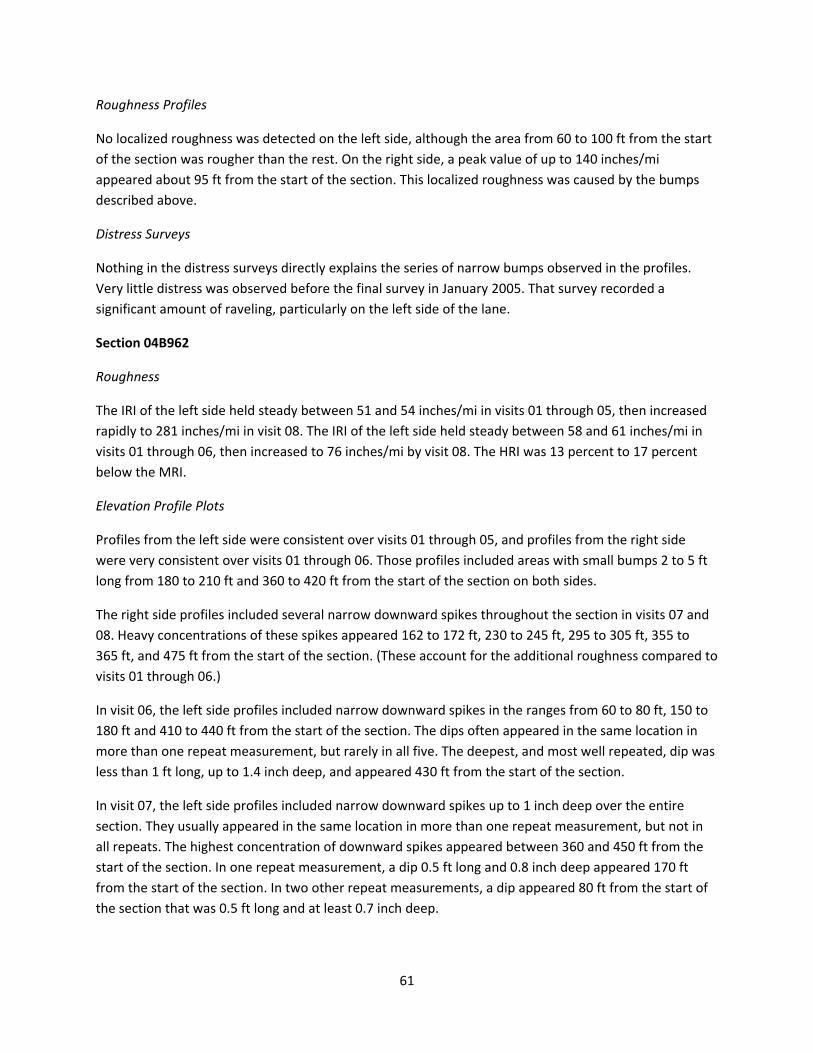
61

Roughness Profiles

No localized roughness was detected on the left side, although the area from 60 to 100 ft from the start

of the section was rougher than the rest. On the right side, a peak value of up to 140 inches/mi

appeared about 95 ft from the start of the section. This localized roughness was caused by the bumps

described above.

Distress Surveys

Nothing in the distress surveys directly explains the series of narrow bumps observed in the profiles.

Very little distress was observed before the final survey in January 2005. That survey recorded a

significant amount of raveling, particularly on the left side of the lane.

Section 04B962

Roughness

The IRI of the left side held steady between 51 and 54 inches/mi in visits 01 through 05, then increased

rapidly to 281 inches/mi in visit 08. The IRI of the left side held steady between 58 and 61 inches/mi in

visits 01 through 06, then increased to 76 inches/mi by visit 08. The HRI was 13 percent to 17 percent

below the MRI.


Profiles from the left side were consistent over visits 01 through 05, and profiles from the right side

were very consistent over visits 01 through 06. Those profiles included areas with small bumps 2 to 5 ft

long from 180 to 210 ft and 360 to 420 ft from the start of the section on both sides.

The right side profiles included several narrow downward spikes throughout the section in visits 07 and

08. Heavy concentrations of these spikes appeared 162 to 172 ft, 230 to 245 ft, 295 to 305 ft, 355 to

365 ft, and 475 ft from the start of the section. (These account for the additional roughness compared to

visits 01 through 06.)

In visit 06, the left side profiles included narrow downward spikes in the ranges from 60 to 80 ft, 150 to

180 ft and 410 to 440 ft from the start of the section. The dips often appeared in the same location in

more than one repeat measurement, but rarely in all five. The deepest, and most well repeated, dip was

less than 1 ft long, up to 1.4 inch deep, and appeared 430 ft from the start of the section.

In visit 07, the left side profiles included narrow downward spikes up to 1 inch deep over the entire

section. They usually appeared in the same location in more than one repeat measurement, but not in

all repeats. The highest concentration of downward spikes appeared between 360 and 450 ft from the

start of the section. In one repeat measurement, a dip 0.5 ft long and 0.8 inch deep appeared 170 ft

from the start of the section. In two other repeat measurements, a dip appeared 80 ft from the start of

the section that was 0.5 ft long and at least 0.7 inch deep.

62

The visit 07 profiles from the left side also included five longer disturbances that were detected in all

five repeat measurements: (1) a 2 ft long, 0.5 inch deep dip centered 418 ft from the start of the section;

(2) a 4 ft long, 0.5 inch deep dip centered 431 ft from the start of the section; (3) a 1.5 ft long, 0.4 inch

high bump 471 ft from the start of the section; (4) a 2 ft long, 0.4 inch high bump 484 ft from the start of

the section; and (5) a 1.5 ft long, up to 0.3 inch high bump 492 ft from the start of the section. All of

these features appeared among a high concentration of narrow downward spikes.

The visit 08 profiles from the left side included many areas with a high concentration of narrow

downward spikes up to 2.5 inches deep, but the spikes rarely appeared in more than the same location

in more than two repeat measurements. The highest concentration of spikes appeared in repeats 4 and

7. The profiles also included some bumps up to 2 ft long and 0.5 inch high in the last 40 ft of the section

and a 4 ft long, 0.5 inch deep dip in the last 5 ft of the section.

Roughness Profiles

Roughness profiles for the right side were very consistent in visits 01 through 06. Although no localized

roughness appeared in these profiles, the distribution of roughness along the section was not very

uniform. The growth in roughness after visit 06 took place over the entire length of the section.

No localized roughness was detected on the left side in visits 01 through 06, although the areas with

small bumps described above were rougher than the surrounding pavement.

In visits 06 and 07, localized roughness (or at least increased roughness) in the left side profiles

appeared about 80 ft from the start of the section in one repeat measurement per visit and about 175 ft

from the start of the section in one or two repeat measurements per visit. These are locations where

deep, narrow dips were found in some, but not all, repeat measurements. Localized roughness also

appeared in visit 06 about 430 ft from the start of the section and in the last 20 ft of the section. Both of

these areas appeared as severe localized roughness in visit 07, with peak values of up to 550 inches/mi

in the roughness profiles.

In visit 08, the left side profiles were very rough over much of the section. (The exception was the area

from 230 to 350 ft from the start of the section.) The most severe localized roughness appeared (1) at

the very end of the section; (2) in one repeat measurement about 20 ft from the start of the section;

and (3) in all but one repeat measurement about 80 ft from the start of the section.

Distress Surveys

The distress survey of January 1999 showed five areas of longitudinal cracking or WP cracking. Many of

these areas correspond to the locations where narrow downward spikes appeared in the left side

profiles from visit 06. In visits 07 and 08, cracking covered the entire left WP (and most of the right WP).

This probably explains the downward spikes that appeared throughout the profiles and the hit‐or‐miss

nature of their distribution.

The distress survey in April 2002 recorded potholes about 427 ft and 434 ft from the start of the section.

The distress survey in January 2005 recorded a large number of potholes and patches in the left WP over

63

the last 100 ft of the section. Their locations corresponded to the locations of longer bumps and dips in

the visit 07 and 08 profiles.

The deep narrow dip in the left side profiles from visits 06 through 08 did not correspond to anything in

the distress surveys beyond the WP cracking found over the entire section.

Section 04B964

Roughness

The IRI increased fairly steadily from 41 to 52 inches/mi on the left side and from 42 to 49 inches/mi on

the right side. The HRI was 11 percent below the MRI in visit 01. The gap between HRI and MRI grew

steadily to 17 percent by visit 08.


The profiles changed very little over the monitoring period with the exception of three rough features.

After visit 02, a dip appeared about 136 ft from the start of the section on the left side. It was

about 1 ft long and grew in depth from 0.15 inch to 0.4 inch over visits 03 through 08. However,

the dip was not present in every repeat measurement.

A dip up to 0.15 inch deep appeared 155 ft from the start of the section’s left side in all visits.

Starting in visit 04, a narrow dip appeared in the right side profiles about 160 ft from the start of

the section. The dip rarely appeared in all five repeat measurements within a visit and ranged in

depth up to 0.25 inch.

Roughness Profiles

Together, the first two dips described above caused an area of localized roughness that grew in severity

to a peak value of 130 inches/mi by visit 08. The increased roughness at this area contributed

significantly to the growth in roughness with time on the left side between visits 01 and 07.

In the most extreme case (visit 04, repeat 01), the third dip described above caused a peak value in the

roughness profile of 106 inches/mi on the right side. Other than the influence of the dip 160 ft from the

start of the section, roughness was very evenly distributed along the section on the right side.

PSD Plots

Although the content was biased toward long wavelengths, some content was isolated around

wavelengths of about 15 to 16 ft on the left side.

64

Distress Surveys

Nothing in the distress surveys directly explains the three narrow dips described above. Very little

distress was observed before April 2002. In April 2002 and January 2005, the distress surveys recorded

raveling along the entire section in both WPs.

SUMMARY

This section summarizes important observations from each pavement section within the SPS‐9A project

limits. Some observations within this report were common to more than one pavement section, as

described below. This section of the report, in conjunction with the roughness progression plots (Figures

17 through 24), provides the essential information about each pavement section.

Profiles from Sections 04B901, 04B902, 04B903, and 04B962 included narrow downward spikes

dispersed throughout their length. The spikes usually appeared in only one or two repeat measurements

at each location. These were caused by cracking, which covered both WPs of Sections 04B901, 04B902,

04B903, and 04B962 in the later visits. The spikes typically first appeared in profile measurements from

November 2001 (visit 06), but were much more prevalent in February and December 2004 (visits 07 and

08). The spikes were usually more severe and numerous in the left side profiles. In Sections 04B901 and

04B902, the spikes were most severe in the left side profiles from visit 07. Although it is not clear why

fewer spikes were detected in visit 08 on those two sections, it may be a consequence of a subtle

difference in profiler positioning. The spikes account for most of the increase in the IRI values,

particularly on the left side, in Sections 04B901, 04B902, 04B903, and 04B962 after November 2001.

Sections 04B902 and 04B962 included several potholes in the left WP that were observed in the distress

survey from January 2005. The profiles in the location of these potholes were rarely consistent among

the five repeat measurements from the last two profiling visits. In Section 04B902, the narrow

downward spikes found throughout the profiles were somewhat more likely to appear near the

potholes than in other locations, but no direct relationship was observed. Bumps appeared near two of

the potholes in two of the five repeat profile measurements in February 2004. This may have been

caused by narrow patching that was only covered by the lateral placement of the profiler in two of the

passes, but no patching was noted. In Section 04B962, two of the seven potholes caused dips about

0.5 ft long and up to 1 inch deep in the last profiling visit that were fairly well repeated.

The final distress survey (January 2005) for Sections 04B901, 04B902, 04B903, 04B960, 04B962, and

04B964 all showed areas of cracking that cover both WPs over the entire section length. In these

instances, fatigue cracking is so prevalent that it is difficult to match individual cracks to roughness

within the measured profile. However, in a few cases, features in the profiles that affected the

roughness were found that correspond directly to the location of transverse cracks noted in the distress

survey. Several narrow dips appeared in Section 04B959 in the final profiling visit that corresponded to

the locations of transverse cracks noted in January 2005. In Section 04B901, a narrow dip appeared in

the right side profiles about 480 ft from the start of the section in the last two profiling visits. This is a

location where transverse cracking was noted in April 2002. An area of localized roughness about 10 ft

long appeared in the last two visits of Section 04B960 that included multiple transverse cracks.

65

Profiler Model

The change in profiler in late 2002 affected the long‐wavelength content of the profiles on every test

section because the newer profiler used a high‐pass filter that eliminated a little more of the profile

content than the previous device. The change in high‐pass filtering methods had no probable effect on

the measurement of localized roughness or the study of narrow bumps and dips caused by distresses.

Another minor device effect within the profiles was peaks in the PSD plots with no pavement‐related

explanation. In visits 01 through 06 (measured by the K.J. Law Engineers T‐6600 profiler), all profiles

from the left and right side included a peak in their spectral content at a wavelength somewhere

between 0.35 and 0.52 ft and another at a wavelength of double the first.

Individual Test Sections

The summaries below provide the most important observations made about each test section. To help

provide context for these summary statements, Figure 25 shows the range of left and right IRI for each

section. Note that the highest IRI value for some of the sections did not occur in the final visit. (See the

appendix or Figures 17 through 24.)

Section 04B901

Although this section started out moderately smooth, with an MRI value of 65 inches/mi, roughness

grew significantly to a final MRI value of 97 inches/mi. While the roughness of the right side grew

steadily, the roughness of the left side reached a peak IRI value of 128 inches/mi in February 2004 and

then reduced to a final value of 90 inches/mi. In the last three profiling visits, the profiles included

narrow downward spikes that often did not appear in the same location in more than one repeat

measurement. The highest concentration of dips appeared in the left side profiles in February 2004,

which accounts for much of the additional roughness over the previous and subsequent visits. Localized

roughness appeared in the right side profiles over the last 25 ft of the section because of 5‐ft‐long

bumps and dips. In 2004, the profiles in this area also often included a 1‐inch deep narrow dip at a

transverse crack 480.5 ft from the start of the section.

Section 04B902

The section was somewhat smooth until 2004. Starting with the profile measurement of November

2001, the profiles included an increasing number of narrow dips, particularly on the left side, that often

did not appear in the same location in more than one repeat measurement. These dips were most

severe in the left side profiles from February 2004, which had an average roughness value of

143 inches/mi, but were not at all consistent with each other. Although the spikes were less severe in

November 2004, the profiles included patches of narrow dips in three areas where potholes were

recorded in the distress surveys.

66

Figure 25. Summary of IRI Ranges

Section 04B903

The right side of this section remained somewhat smooth throughout the monitoring history, but the

left side IRI more than doubled between visits 06 and 08. Starting in visit 06, the profiles included an

increasing number of narrow dips, particularly on the left side, that often did not appear in the same

location in more than one repeat measurement. In visit 07, a deep (2.4‐inch) narrow dip appeared 122 ft

from the start of the section on the left side. A deep (2‐inch) narrow dip appeared 333 ft from the start

of the section in three of the five repeat measurements from visit 08 on the left side. Both dips caused

severe localized roughness. Roughness at the dip in visit 08 accounted for the high (15.4 inches/mi)

standard deviation in the left side IRI from visit 08.

0 50 100 150 200 250 300IRI (in/mi)

B964 LR

B962 LR

B961 LR

B960 LR

B959 LR

B903 LR

B902 LR

B901 LR

IRI (inches/mile)

04B901

04B902

04B903

04B959

04B960

04B961

04B962

04B964

67

Section 04B959

This section remained smooth throughout the monitoring period, although the MRI progressed by

13 inches/mi. An area of localized roughness appeared on the left side at the start of the section

because of a long dip and some rough features just ahead of the section start. The roughness of the

right side was uniform along the section, until the roughness progressed significantly in the first third of

the section because of the influence of cracking.

Section 04B960

The MRI increased from 46 to 51 inches/mi over the monitoring period. An area of localized roughness

appeared on the left side about 445 ft from the start of the section by the end of the monitoring period.

A sunken area of pavement, including three narrow dips about 0.2 inch deep at transverse cracks,

caused the roughness. This area accounts for most of the roughness progression of the entire section.

Section 04B961

The MRI ranged from 55 to 59 inches/mi over the entire monitoring period. An area of increased

roughness appeared on the right side of the lane 60 to 100 ft from the start of the section because of a

series of short, narrow bumps in the profiles. The bumps appeared on the left side of the lane also, but

they did not increase the roughness as much there. The bumps were very consistently measured over

the monitoring period.

Section 04B962

This section remained smooth until 2004, when the final MRI value was 178 inches/mi, more than three

times the initial value of 55 inches/mi. The sharp increase in roughness occurred primarily within the left

side profiles. By the final visit, the left side profiles were strongly affected by roughness at potholes and

patching, and included a high concentration of deep, narrow downward spikes caused by cracking in the

WP. Most of the potholes and patches appeared in the last 100 ft of the section.

Section 04B964

The MRI increased from 41 to 50 inches/mi over the monitoring period. The majority of the roughness

progression on this section was caused by three narrow dips that grew in severity with time: (1) 136 ft

from the start of the section on the left side, (2) 155 ft from the start of the section on the left side, and

(3) 160 ft from the start of the section on the right side.

69

CHAPTER 5. CONCLUSIONS AND RECOMMENDATIONS

ADOT initiated the SPS‐9A project to study the relative performance of the Superpave binders compared

to the commonly used agency binders, which will provide a foundation for future design decisions.

Surface distress, deflection, and profile data were used as the basis for performance evaluation and

were analyzed as part of the study.

The SPS‐9A project offers a unique opportunity to directly compare performance of various asphalt

binders while reducing the confounding effect of other variables such as traffic‐loading, climate, and

subgrade conditions. However, findings drawn from this evaluation must be considered carefully. The

experiment design did not offer replicate treatments to verify findings. Conclusions drawn from this

comparison are based on one set of in situ conditions; observations from other climate or loading

scenarios may differ from those noted within this report. Therefore, findings reported may be unique to

the conditions and construction of this site.

Despite these issues, the data captured at the project provides valuable insight into pavement

performance, design, management, and construction. Following is a summary of lessons learned from

the performance data collected at the SPS‐9A site:

Roughness and roughness progression alone cannot be used to represent the health of a test

section. Several test sections did not exhibit changes in roughness in proportion to the amount

of fatigue cracking, and sections that had clearly reached the end of their service lives did not

necessarily have roughness values that would trigger a rehabilitation event.

Most every section except Section 04B959 (SMA polymer with ACFC) and Section 04B961 (SMA

polymer with cellulose) showed significant growth in fatigue and longitudinal cracking 10 years

after construction.

Where fatigue cracking was very prevalent, it was difficult to match individual cracks to

roughness within the measured profile. However, in a few cases, features in the profiles that

affected the roughness corresponded directly to the location of transverse cracks noted in the

distress survey.

Construction quality can play a major role in performance. The construction observations

documented in the LTPP construction report were limited to Superpave sections (Sections

04B902 and 04B903) and the agency standard mix section (Section 04B901). However, it showed

that all three sections were free of any construction issues.

Half of the sections (04B901, 04B959, 04B960, 041007/04B962) had reasonable patterns of

environmental distress growth with a clear increase in magnitude approximately 10 years after

construction. Section 04B964 had little environmental distress growth for seven years and then

rapidly increased after 10 years.

70

With no replicate sections, researchers had limited ability to assess potential variability

independent of actual performance.

For the SP‐1 mix designs (Sections 04B902 and 04B903), the PG 70‐10 binder (Section 04B903)

performed significantly better, both structurally and environmentally, than the PG 76‐10 binder

(Section 04B902). It also performed significantly better than the standard agency mix at resisting




SMA with cellulose fibers was, by far, the best pavement mix at resisting both structural and

environmental deterioration. From a roughness perspective, the SMA and ARAC sections

outperformed the Superpave mixes.

Based on these findings, the research team recommends the following:

Most of the pavement test sections appeared to have experienced top‐down cracking; however,

this could not be confirmed. It is recommended that forensic analysis be performed at other

locations throughout Arizona to learn about the factors contributing to top‐down cracking.

If the SMA with cellulose is sufficiently cost‐effective, ADOT should consider expanding its use in

overlay applications.

71

REFERENCES

American Association of State Highway and Transportation Officials (AASHTO). 1993. AASHTO Guide for

Design of Pavement Structures. Washington, D.C.: American Association of State Highway and

Transportation Officials.

Evans, L. D. and A. Eltahan. 2000. LTPP Profile Variability. Publication FHWA‐RD‐00‐113. McLean, VA:

Federal Highway Administration: 178.

Federal Highway Administration (FHWA). 1998. “Arizona SPS‐9, I‐10 Westbound Milepost 112‐123,

Construction Report on Site 04B900, Arizona Department of Transportation, Final.”

Huang, Y. H. 1993. Pavement Analysis and Design. Englewood Cliffs, NJ: Prentice‐Hall.

Karamihas, S. M. 2004. “Development of Cross Correlation for Objective Comparison of Profiles.”

International Journal of Vehicle Design 36(2/3): 173–193.

Karamihas, S. M., T. D. Gillespie, and S. M. Riley. 1995. “Axle Tramp Contribution to the Dynamic Wheel

Loads of a Heavy Truck.” Proceedings of the 4th International Symposium on Heavy Vehicle Weights and

Dimensions, Ann Arbor, MI. C. B. Winkler (ed.): 425–434.

Kim, Y. Richard, B. Underwood, M. Sakhaei Far, N. Jackson, and J. Puccinelli. 2011. LTPP Computed

Parameter: Dynamic Modulus. Publication FHWA‐HRT‐10‐035. Washington, D.C.: Federal Highway

Administration.

Mahoney, J. 1995. WSDOT Pavement Guide, Volume 2: Pavement Notes. Olympia: Washington State

Department of Transportation.

Miller, J. S. and W. Y. Bellinger. 2003. Distress Identification Manual for the Long‐Term Pavement

Performance Program. Revised fourth edition. Publication FHWA‐RD‐03‐031. Washington, D.C.: Federal

Highway Administration.

Rada, G. R., C. L. Wu, R. K. Bhandari, A.R. Shekharan, G. E. Elkins, and J. S. Miller. 1999. Study of LTPP

Distress Data Variability, Volume I. Publication FHWA‐RD‐99‐074. Washington, D.C.: Federal Highway

Administration.

Sayers, M. W. 1989. “Two Quarter‐Car Models for Defining Road Roughness: IRI and HRI.”

Transportation Research Record: Journal of the Transportation Research Board 1215: 165–172.

Sayers, M. W. 1990. “Profiles of Roughness.” Transportation Research Record: Journal of the

Transportation Research Board 1260: 106–111.

Sayers, M. W. and S. M. Karamihas. 1996a. “Estimation of Rideability by Analyzing Longitudinal Road

Profile.” Transportation Research Record: Journal of the Transportation Research Board 1536: 110–116.

72

Sayers, M. W. and S. M. Karamihas. 1996b. Interpretation of Road Roughness Profile Data. Publication

FHWA‐RD‐96‐101 (Washington, D.C.: Federal Highway Administration): 177.

Simpson, A. L. 2001. Characterization of Transverse Profiles. Publication FHWA‐RD‐01‐024. Washington,

D.C.: Federal Highway Administration.

73

APPENDIX: ROUGHNESS VALUES

This appendix lists the left International Roughness Index (IRI), right IRI, mean roughness index (MRI),

Half‐car Roughness Index (HRI), and Ride Number (RN) values for each visit of each section. The

roughness values are the average for five repeat runs. The five runs were selected from a group of as

many as nine by automated comparison of profiles, as described in the report. Values of standard

deviation are also provided for left and right IRI to reveal cases of high variability among the five

measurements. However, the screening procedure used to select five repeats usually helped reduce the

level of scatter.

The discussion of roughness in the report emphasizes the left and right IRI. Nevertheless, the other

indexes do provide useful additional information. MRI is simply the average of the left and right IRI

value. HRI is calculated by converting the IRI filter into a half‐car model (Sayers 1989) by collapsing the

left and right profile into a single profile in which each point is the average of the corresponding left and

right elevation. The IRI filter is then applied to the resulting signal. The HRI is very similar to the IRI

except that side‐to‐side deviations in profile are eliminated. The result is that the HRI value for a pair of

profiles will always be lower than the corresponding MRI value. Comparing the HRI and MRI value

provides a crude indication of the significance of roll (i.e., side‐by‐side variation in profile) to the overall

roughness. When HRI is low compared to MRI, roll is significant. This is common among asphalt

pavements (Karamihas et al. 1995). Certain types of pavement distress, such as longitudinal cracking,

may also cause significant differences between HRI and MRI.

Figure 26 compares the HRI to MRI for all of the profile measurements that are covered in this appendix

(290 pairs of roughness values). The figure shows a best fit line with a zero intercept and a line of

equality. The slope of the line is 0.845, which is typical for asphalt pavement.

RN has shown a closer relationship to road user opinion than the other indexes (Sayers and Karamihas

1996a). As such, it may help distinguish the segments from each other by ride quality. Further, the effect

on RN may help quantify the impact of that distress on ride when a particular type of distress dominates

the roughness of a section. In particular, a very low RN value coupled with moderate IRI values indicates

a high level of short wavelength roughness and potential sensitivity to narrow dips and measurement

errors caused by coarse surface texture.

Table 21 provides the roughness values. The table also lists the date of each measurement and the time

in years since the site was opened to traffic. Negative values indicate measurements that were made

before rehabilitation.

74

Figure 26. Comparison of HRI to MRI

Table 21. Roughness Values

Section Date Years Left IRI (inch/mi)

Right IRI (inch/mi)

MRI HRI RN

Ave St Dev Ave St Dev (inch/mi) (inch/mi) 04B901 29‐Jan‐97 1.84 66 1.0 65 1.2 65 58 3.79 04B901 5‐Dec‐97 2.68 68 1.5 63 1.5 65 57 3.67 04B901 7‐Dec‐98 3.69 66 1.1 68 1.2 67 59 3.68 04B901 10‐Nov‐99 4.61 68 1.0 66 1.9 67 58 3.72 04B901 12‐Nov‐01 6.62 77 2.1 70 2.1 74 63 3.51 04B901 9‐Feb‐04 8.86 128 4.9 88 4.2 108 88 2.41 04B901 17‐Dec‐04 9.71 90 4.2 103 4.1 97 77 2.82 04B902 29‐Jan‐97 1.84 58 1.3 61 1.4 60 50 3.87 04B902 5‐Dec‐97 2.68 56 1.6 59 1.1 58 49 3.82 04B902 7‐Dec‐98 3.69 54 0.8 61 0.5 58 49 3.82 04B902 10‐Nov‐99 4.61 63 3.1 61 0.7 62 53 3.68 04B902 12‐Nov‐01 6.62 73 10.3 63 0.6 68 57 3.46 04B902 9‐Feb‐04 8.86 143 28.1 69 2.9 106 86 2.56 04B902 17‐Dec‐04 9.71 79 2.3 89 0.6 84 66 2.94 04B903 29‐Jan‐97 1.84 59 0.6 69 1.1 64 54 3.77 04B903 5‐Dec‐97 2.68 59 1.8 67 0.5 63 53 3.71 04B903 7‐Dec‐98 3.69 60 0.5 68 1.0 64 54 3.73 04B903 10‐Nov‐99 4.61 60 0.9 68 1.0 64 53 3.80 04B903 12‐Nov‐01 6.62 66 3.2 67 1.3 66 54 3.69 04B903 9‐Feb‐04 8.86 119 1.8 68 1.9 93 75 2.37 04B903 17‐Dec‐04 9.71 143 15.4 71 2.9 107 87 2.42

0

50

100

150

200

0 50 100 150 200

HRI = 0.845•MRI

Line of Equality

HRI (in/mi)

MRI (in/mi)MRI (inches/mile)

HRI (inches/mile)

75

Table 21. Roughness Values (Continued)

Section Date Years Left IRI (inch/mi)

Right IRI (inch/mi)

MRI HRI RN

Ave St Dev Ave St Dev (inch/mi) (inch/mi) 04B959 29‐Jan‐97 1.84 43 0.6 51 0.7 47 41 4.22

04B959 5‐Dec‐97 2.68 45 0.6 53 0.7 49 43 4.08

04B959 7‐Dec‐98 3.69 46 0.5 55 0.8 50 44 4.09

04B959 10‐Nov‐99 4.61 47 0.5 55 1.1 51 44 4.13

04B959 12‐Nov‐01 6.62 47 0.6 61 1.1 54 46 4.10

04B959 9‐Feb‐04 8.86 50 0.9 60 1.4 55 46 3.95

04B959 17‐Dec‐04 9.71 47 1.1 73 4.2 60 51 3.81

04B960 29‐Jan‐97 1.84 47 1.1 45 0.9 46 39 4.07

04B960 5‐Dec‐97 2.68 47 0.6 46 0.7 46 39 3.95

04B960 7‐Dec‐98 3.69 45 1.0 46 0.8 46 39 3.99

04B960 10‐Nov‐99 4.61 47 0.7 46 0.6 47 40 4.05

04B960 12‐Nov‐01 6.62 46 0.6 45 0.4 46 40 4.06

04B960 9‐Feb‐04 8.86 52 0.7 48 0.7 50 41 3.75

04B960 17‐Dec‐04 9.71 54 1.3 47 1.1 51 42 3.66

04B961 29‐Jan‐97 1.84 52 0.3 58 0.6 55 49 4.00

04B961 5‐Dec‐97 2.68 56 0.8 56 0.6 56 50 3.86

04B961 7‐Dec‐98 3.69 55 1.5 59 1.7 57 51 3.88

04B961 10‐Nov‐99 4.61 52 1.0 60 0.9 56 50 3.99

04B961 12‐Nov‐01 6.62 54 1.1 57 0.4 55 50 3.97

04B961 9‐Feb‐04 8.86 56 1.1 58 0.4 57 51 3.82

04B961 17‐Dec‐04 9.71 59 2.8 59 1.3 59 52 3.77

04B962 29‐Jan‐97 1.83 52 1.9 59 2.0 55 48 3.84

04B962 2‐Feb‐97 1.84 51 1.0 58 0.7 54 47 3.86

04B962 5‐Dec‐97 2.68 54 2.0 60 0.9 57 50 3.71

04B962 7‐Dec‐98 3.69 53 1.4 61 1.6 57 49 3.73

04B962 10‐Nov‐99 4.61 54 1.7 58 0.9 56 49 3.79

04B962 12‐Nov‐01 6.62 81 5.5 59 1.1 70 58 3.06

04B962 9‐Feb‐04 8.86 149 12.3 72 1.8 111 92 2.26

04B962 17‐Dec‐04 9.71 281 49.8 76 3.0 178 152 1.77

04B964 29‐Jan‐97 1.83 41 0.3 42 0.9 41 37 4.24

04B964 2‐Feb‐97 1.84 41 0.8 40 0.5 41 36 4.23

04B964 5‐Dec‐97 2.68 45 1.2 41 0.5 43 37 4.02

04B964 7‐Dec‐98 3.69 44 0.4 47 1.5 45 38 4.03

04B964 10‐Nov‐99 4.61 46 0.8 46 1.4 46 39 4.02

04B964 12‐Nov‐01 6.62 47 0.8 46 0.6 47 40 4.01

04B964 9‐Feb‐04 8.86 49 1.4 47 1.1 48 41 3.79

04B964 17‐Dec‐04 9.71 52 1.8 49 2.4 50 41 3.76

performance evaluation of arizona’s ltpp sps-9 project · us department of transportation ......

Documents