performance erification tatement for …€¦ · for precision measurement engineering minidot...
TRANSCRIPT
Ref. No. [UMCES] CBL 2016-011 ACT VS16-02
1
PERFORMANCE VERIFICATION STATEMENT
For Precision Measurement Engineering miniDOT Dissolved Oxygen Sensors
TECHNOLOGY TYPE: Dissolved Oxygen sensors APPLICATION: In situ estimates of DO for coastal moored deployments PARAMETERS EVALUATED: Response linearity, accuracy, precision and reliability
TYPE OF EVALUATION: Laboratory and Field Performance Verification DATE OF EVALUATION: Testing conducted from January 2015 to January 2016 EVALUATION PERSONNEL: T. Johengen, G.J. Smith, D. Schar, H. Purcell, D. Loewensteiner, Z.
Epperson, and M. Tamburri, G. Meadows, S. Green, F. Yousef, J. Anderson.
NOTICE:
ACT verifications are based on an evaluation of technology performance under specific, agreed-upon protocols, criteria, and quality assurance procedures. ACT and its Partner Institutions do not certify that a technology will always operate as verified and make no expressed or implied guarantee as to the performance of the technology or that a technology will always, or under circumstances other than those used in testing, operate at the levels verified. ACT does not seek to determine regulatory compliance; does not rank technologies nor compare their performance; does not label or list technologies as acceptable or unacceptable; and does not seek to determine “best available technology” in any form. The end user is solely responsible for complying with any and all applicable federal, state, and local requirements. This document has been peer reviewed by ACT Partner Institutions and a technology-specific advisory committee and was recommended for public release. Mention of trade names or commercial products does not constitute endorsement or recommendation by ACT for use. Questions and comments should be directed to: Dr. Tom Johengen ACT Chief Scientist CILER- University of Michigan 4840 S. State Street Ann Arbor, MI 48108 USA Email: [email protected]

Ref. No. [UMCES] CBL 2016-011 ACT VS16-02
2
TABLE OF CONTENTS
EXECUTIVE SUMMARY .......................................................................................................... 3
BACKGROUND AND OBJECTIVES ....................................................................................... 5
INSTRUMENT TECHNOLOGY TESTED .............................................................................. 6
PERFORMANCE EVALUATION TEST PLAN ...................................................................... 6
LABORATORY TESTS ..................................................................................................................... 6
MOORED FIELD TESTS ................................................................................................................... 8
REFERENCE SAMPLE ANALYSIS ................................................................................................... 11
RESULTS OF LABORATORY TEST ..................................................................................... 13
RESULTS OF MOORED FIELD TESTS ................................................................................ 29
MOORED DEPLOYMENT AT MICHIGAN TECH GREAT LAKES RESEARCH CENTER .......................... 30
MOORED DEPLOYMENT AT CHESAPEAKE BIOLOGICAL LABORATORY ........................................ 35
MOORED DEPLOYMENT OFF COCONUT ISLAND IN KANEOHE BAY, HAWAII ................................. 40
PROFILING DEPLOYMENT IN THE GREAT LAKES ......................................................................... 46
QUALITY ASSURANCE/QUALITY CONTROL ................................................................. 53
REFERENCES ............................................................................................................................ 57
ACKNOWLEDGEMENTS ....................................................................................................... 58
MANUFACTURER’S RESPONSE .......................................................................................... 59
Ref. No. [UMCES] CBL 2016-011 ACT VS16-02
3
EXECUTIVE SUMMARY
The Alliance for Coastal Technology (ACT) conducted a sensor verification study of in situ dissolved oxygen sensors during 2015-2016 to characterize performance measures of accuracy and reliability in a series of controlled laboratory studies and field mooring tests in diverse coastal environments. The verification including several months of Laboratory testing along with three field deployments covering freshwater, estuarine, and oceanic environments. Laboratory tests of accuracy, precision, response time, and stability were conducted at Moss Landing Marine Lab. A series of nine accuracy and precision tests were conducted at three fixed salinity levels (0, 10, 35) at each of three fixed temperatures (5, 15, 30 oC). A laboratory based stability test was conducted over 56 days using deionized water to examine performance consistency without active biofouling. A response test was conducted to examine equilibration times across an oxygen gradient of 8mg/L at a constant temperature of 15 oC. Three field-mooring tests were conducted to examine the ability of test instruments to consistently track natural changes in dissolved oxygen over extended deployments of 12-16 weeks. Deployments were conducted at: (1) Lake Superior, Houghton, MI from 9Jan – 22Apr, (2) Chesapeake Bay, Solomons, MD from 20May – 5Aug, and (3) Kaneohe Bay, Kaneohe, HI from 24Sep – 21Jan. Instrument performance was evaluated against reference samples collected and analyzed on site by ACT staff using Winkler titrations following the methods of Carignan et.al. 1998. A total of 725 reference samples were collected during the laboratory tests and between 118 – 142 reference samples were collected for each mooring test. This document presents the performance results of PME miniDOT dissolved oxygen sensor using optical luminescence technology.
Instrument accuracy and precision for the PME miniDOT was tested under nine combinations of temperature and salinity over a range of DO concentrations from 10% to 120% of saturation. The means of the difference between the miniDOT and reference measurement ranged from -0.339 to 0.126 mg/L over all nine trials. There were no consistent trends in instrument accuracy across salinity ranges. There was a noticeable change in the direction of the offset across temperature ranges with the average offset equal to -0.23 mg/L for the 4 and 15 oC trials compared to a mean offset of 0.11 mg/L for the 30 oC trials. A linear regression of instrument and reference measurements for all trials combined data (n=334; r2 = 0.973; p<0.0001) produced a slope of 0.98 and intercept of 0.020. Instrument offsets and the linear regression omitted comparisons that were clearly impacted by contamination of bubbles of the sparging gas that were trapped on the sensor foil due to its orientation within the tank. The absolute precision, estimated as the standard deviation (s.d.) around the mean, ranged from 0.005 – 0.013 mg/L across trials with an overall average of 0.008 mg/L. Relative precision, estimated as the coefficient of variation (CV% = (s.d./mean)x100), ranged from 0.057 – 0.248 percent across trials with an overall average of 0.098%. Instrument accuracy was assessed under a 56 day lab stability test in a deionized water bath cycling temperature and ambient DO saturation on a daily basis. The overall mean difference between measurements was 0.034 (s.d. = 0.107) mg/L for 77 comparisons (out of a potential total of 77). There was a small but statistically significant trend in accuracy over time (slope = -0.002 mg/L/d; r2 = 0.11; p=0.003) indicating very modest performance drift over the 56 days.

Ref. No. [UMCES] CBL 2016-011 ACT VS16-02
4
A functional response time test was conducted by examining instrument response when rapidly transitioning between adjacent high (9.6 mg/L) and low (2.0 mg/L) DO water baths, maintained commonly at 15 oC. The calculated τ90 was 90 s during high to low transitions and 63 s for low to high transitions covering the 8 mg/L DO range.
At Houghton, MI a field deployment test was conducted under the ice over 104 days with a mean temperature and salinity of 0.7 oC and 0.01. The PME miniDOT operated successfully throughout the entire 15week deployment and generated 9859 observations based on its 15 minute sampling interval for a data completion result of 100%. It should be noted that for this deployment a wiping system was not yet available, so some caution should be used in comparisons against the other field test results. The average and standard deviation of the measurement difference over the total deployment was 0.029 ± 0.072 mg/L with a total range of -0.307 to 0.205mg/L. The drift rate of instrument offset, estimated by linear regression (r2=0.373; p<0.0001), was 0.001 mg/L/d. This rate would include any biofouling effects as well as any electronic or calibration drift. A linear regression of the instrument versus reference measurements over the first month (r2 = 0.97; p<0.0001) produced a slope of 0.92 and intercept of 1.03.
At Chesapeake Biological Lab, a field deployment test was conducted over 78 days with a mean temperature and salinity of 25.6 oC and 10.9. The PME miniDOT generated 21,810 observations over the 11 week deployment based on its 5 minute sampling interval; however, only 18,173 of the measurements were considered acceptable based on values that were less than 2 mg/L from any minimum reference sample over a similar timeframe and less than 2 mg/L from continuously monitored DO from a nearby independent data sonde. The accepted data resulted in a data completion rate for this deployment of 83%. The average and standard deviation of the difference between instrument and reference measurements for the deployment was -0.40 ±0.702 mg/L, with the total range of differences between -1.90 to 0.86 mg/L. The calculated drift rate in instrument response for the entire deployment period (using the accepted data) was -0.026 mg/L/d (r2 = 0.83; p<0.001). If we consider only the first 35 days of the deployment before any indication of a malfunction, the drift rate was only -0.009 mg/L/d (r2 = 0.34; p<0.001). A linear regression of the instrument versus reference measurements for the first month (r2 = 0.98; p<0.001) produced a slope of 0.968 and intercept of 0.306. At Kaneohe Bay, HI a field deployment test was conducted over 121 days with a mean temperature and salinity of 25.8 and 33.4 oC. The PME miniDOT reported 16,957 observations based on its 10 minute sampling interval over the 17 week deployment. Only two instrument value fell outside of an acceptable data range based on ± 2mg/L from any min-max reference sample for essentially a 100% data completion result. The average and standard deviation of the differences between instrument and reference readings (limited to ± 2.0 mg/L DO; n=128 of 129 potential observations) were 0.201 ± .426 mg/L, with a total range in the differences of -1.7021 to 1.441 mg/L. There was a small, but statistically significant, drift in instrument offset (slope = 0.003 mg/L/d; r2 = 0.05; p=0.009) throughout the deployment period. A linear regression of the instrument versus reference measurements for the first month (r2 = 0.97; p<0.001) had a slope of 1.052 and intercept of -0.258.
Overall, the response of the PME miniDOT response showed good linearity overall all three salinity ranges including freshwater, brackish water, and oceanic water; but with slightly higher variability for the oceanic test in Kaneohe Bay. Good agreement between instrument and reference measurements was observed over a wide range of DO conditions varying between 4 to
Ref. No. [UMCES] CBL 2016-011 ACT VS16-02
5
14 mg/L. A linear regression of the composited data (r2 = 0.998; p<0.0001)) had a slope of 0.987 and intercept of -0.150.
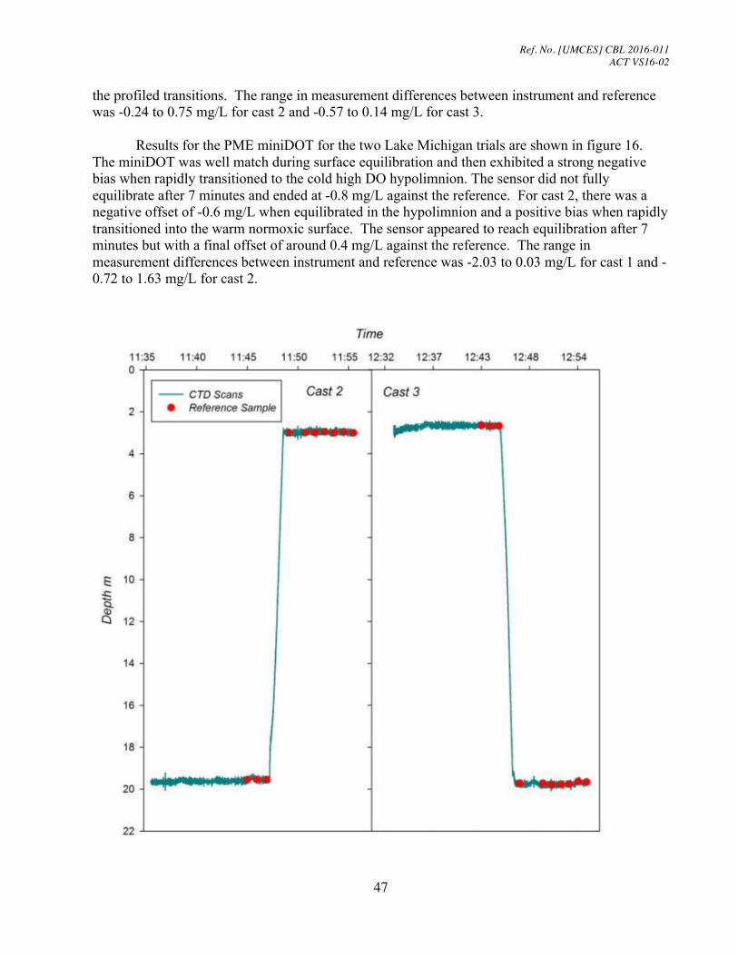
The PME miniDOT was evaluated in a profiling field test in the Great Lakes at two separate locations in order to experience transitions from surface waters into both normoxic and hypoxic hypolimnion. In Muskegon Lake, the temperature ranged from 21.0 oC at the surface to 13.5 oC in the hypolimnion, with corresponding DO concentrations of 7.8 and 2.8 mg/L, respectively. In Lake Michigan, the temperature ranged from 21.0 oC at the surface to 4.1 oC in the hypolimnion, with corresponding DO concentrations of 8.6 and 12.6 mg/L, respectively. Two profiling trials were conducted at each location. The first trial involved equilibrating test instruments at the surface (3m) for ten minutes and then collecting three Niskin bottle samples at one minute intervals. Following the third sample, the rosette was quickly profiled into the hypolimnion where samples were collected immediately upon arrival and then each minute for the next 6 minutes. The second trial was performed in the reverse direction. For Muskegon Lake, the miniDOT exhibited a negative bias in the colder, low DO hypolimnion and a positive bias in the warm, normoxic surface water over both of the trials. The miniDOT appeared to reach equilibration after 7 minutes but still exhibited final offsets of approximately 0.2 mg/L following the profiled transitions. The range in measurement differences between instrument and reference was -0.24 to 0.75 mg/L for cast 2 and -0.57 to 0.14 mg/L for cast 3 (cast 1 was aborted and redone as cast 3). For Lake Michigan, during cast 1 the miniDOT was well matched during surface equilibration and then exhibited a strong negative bias when rapidly transitioned to the cold high DO hypolimnion. The sensor did not fully equilibrate after 7 minutes and ended at -0.8 mg/L against the reference. For cast 2, there was a negative offset of -0.6 mg/L when equilibrated in the hypolimnion and a positive bias when rapidly transitioned into the warm normoxic surface. The sensor appeared to reach equilibration after 7 minutes but with a final offset of around 0.4 mg/L against the reference. The range in measurement differences between instrument and reference was -2.03 to 0.03 mg/L for cast 1 and -0.72 to 1.63 mg/L for cast 2. BACKGROUND AND OBJECTIVES
Instrument performance verification is necessary so that effective existing technologies can be recognized and so that promising new technologies can be made available to support coastal science, resource management and ocean observing systems. To this end, the NOAA-funded Alliance for Coastal Technologies (ACT) serves as an unbiased, third party testbed for evaluating sensors and sensor platforms for use in coastal environments. ACT also serves as a comprehensive data and information clearinghouse on coastal technologies and a forum for capacity building through workshops on specific technology topics (visit www.act-us.info).
As part of our service to the coastal community, ACT conducted a performance verification of commercially available, in situ dissolved oxygen (DO) sensors through the evaluation of objective and quality assured data. The goal of ACT’s evaluation program is to provide technology users with an independent and credible assessment of instrument performance in a variety of environments and applications. To this end, the data and information on performance characteristics were focused on the types of information users most need.
The fundamental objectives of this Performance Verification were to: (1) highlight the potential capabilities of particular in situ DO sensors by demonstrating their utility in a range of coastal environments; (2) verify the claims of manufacturers on the performance characteristics of commercially available DO sensors when tested in a controlled laboratory setting, and (3) verify
Ref. No. [UMCES] CBL 2016-011 ACT VS16-02
6
performance characteristics of commercially available DO sensors when applied in real world applications in a diverse range of coastal environments.
INSTRUMENT TECHNOLOGY TESTED
The Precision Measurement Engineering (PME) miniDOT uses an optical method of determining oxygen concentration. This method takes advantage of the oxygen ‘quenching’ effect that is observed of certain types of fluorescent materials. Photons of excitation light entering these materials transfer energy, excite, electrons of the molecules that make up the materials. These excited electrons briefly occupy higher energy levels but ultimately return to their normal, rest, state. There are at least two paths by which these electrons can lose their excited energy and return to rest. One path is to emit photons. Another path is to lose the energy by transfer to an oxygen molecule. This non-emissive energy loss is the quenching effect.
The presence of oxygen provides a non-emissive path and thereby reduces the intensity of emission. Also, by providing this path oxygen reduces the average length of time that electrons remain in the excited state. So there are two approaches to measuring the amount of oxygen present: measure the intensity of emission or measure the lifetime of emission.
Optical oxygen sensors typically use emission lifetime to sense oxygen. This is because the lifetime is not as sensitive to various problems that can affect the emission intensity. For example as the excitation light source ages it can emit less excitation light. This doesn’t affect the lifetime but does affect the emission light intensity, less excitation light resulting in less emitted light. There are a host of other circuit and physical problems that likewise can affect emitted light intensity.
The miniDOT makes both lifetime and intensity measurement at each measurement time. The DO value recorded by the miniDOT is determined from the emission lifetime. However, miniDOT software also computes the DO determined from the emission intensity. miniDOT records both DO and also the ratio (DO determined from lifetime / DO determined from intensity) at every measurement. Patent Pending. This DO ratio should ideally be 1 and in practice is usually very close to 1.0. If this ratio deviates significantly from 1.0 it can indicate various measurement problems. This unique feature provides a quality estimate for each DO measurement miniDOT records.
PERFORMANCE EVALUTION TEST PLAN Laboratory Tests
Laboratory tests of accuracy, precision, response time, and stability were conducted at Moss Landing Marine Lab. All tests were run under ambient pressure (logged hourly from a barometer at the laboratory) and involved the comparison of dissolved oxygen concentration reported by the instrument versus Winkler titration values of water samples taken from the test baths. All tests were run in thermally controlled tanks at specific temperature, salinity, and DO concentrations. Tanks were well mixed with four submersible Aquatic Ecosystem Model 5 pumps with flow rates of 25 L/min. Temperatures were controlled to within approximately 0.2oC of set point using Thermo Digital One Neslab RTE 17 circulating thermostats flowing through closed coils distributed within the tank. Four RBR temperature loggers were deployed within the tank to verify actual temperature to better than 0.02oC. Salinity was varied by addition of commercial

Ref. No. [UMCES] CBL 2016-011 ACT VS16-02
7
salts (Instant Ocean) to Type 1 deionized water. Salinity was verified at the beginning and end of each test condition by analysis on a calibrated CTD. Dissolved oxygen concentrations were controlled by use of compressed gases of known oxygen concentration sparging through diffusers within the tank. Tanks were covered with a layer of floating closed-cell plastic insulation that continuously sealed the water surface and to minimize atmospheric exchange. If required by the manufacturer, instruments were only calibrated prior to the start of the first lab test, and then again prior to the stability test which began one month later. The following series of tests were conducted in the laboratory trials:
Accuracy at various T/S and DO conditions
A series of measurements were conducted under 36 discrete conditions to target 3 temperatures, 3 salinities, and at least 4 DO concentrations as follows:
• Temperature Conditions: 5, 15, 30oC • 3 Salinity Conditions: 0, 10, 34 • Dissolved oxygen,(% air saturation): 0% (hypoxic), 20 – 30%, 100% and >120%, (levels were
achieved by mixing pure O2 and N2 sources with pure N2 was used for the 0% O2 concentration)
Tests were run such that all 4-6 DO concentrations were tested for a fixed temperature and salinity on the same day. The tests began at ambient, near air saturation, conditions following overnight equilibration of tank water to the test salinity and temperature. Subsequently DO were dropped to near 0 mg/L and increased stepwise to the highest concentration. Instruments were allowed to equilibrate at the fixed temperature and salinity for 1 h before the start of that day’s trial. Sparging with each DO gas concentration was conducted for a minimum of 60 minutes prior to the start of data collection and reference sampling. For each test condition, the test instruments were programmed to sample at no slower than 1 minute intervals and reference samples were collected at 6 timepoints spaced 5 minutes apart for each of the fixed conditions. For three of the timepoints duplicate samples were collected from two different sampling ports mounted at opposite ends of the tank to access heterogeneity within the tank. Inlets of sampling ports were positioned at the depth of the sensor heads (ca. -0.5m). All reference samples were collected while the gas sparging was off and took approximately 1 minute to complete. Reference samples were processed and analyzed as defined below. The order of the test conditions were 15 then 5 then 30oC, going from 0 then 10 then 34 salinity at each temperature. Precision Test at various DO concentrations
Instrument precision was evaluated under stable conditions generally achieved at the start of each trial’s day. Instruments were equilibrated to each test condition for a minimum of one hour prior to testing. The sampling frequency for test instruments was 1 minute with reference samples matching instrument sampling to monitor for drift in tank DO. At least 6 reference samples were collected over a 30 minute instrument precision evaluation trial. Reference samples were processed and analyzed as defined below. Functional Response Time Test
A response time test was conducted by examining measurements during a rapid exchange across a large gradient in dissolved oxygen for a fixed temperature (15 oC) in deionized water, following the approach described in Bittig et al. 2014. The reservoirs of the thermostat baths were
Ref. No. [UMCES] CBL 2016-011 ACT VS16-02
8
constantly bubbled with either N2 gas or air to maintain discrete DO levels. A submersible pump was added to each bath to ensure uniform flow and oxygen conditions and instruments were mounted at a fixed position within the baths to minimize variance due to instrument manipulation. Instruments were programmed to measure every 5s continuously for eight minutes following the exchange. For instruments with the capability, real-time monitoring of instrument output was monitored to verify a steady state reading had been obtained. Instruments were moved from the high DO concentration to the low DO concentration and subsequently reversed to check for response hysteresis. During transitions, care was taken to minimize carryover by shaking off residual water. The sensor was then carefully inserting into the new bucket and mixed by hand to ensure no bubble entrapment and full exposure to the new solution. Reference samples from each reservoir were taken at the beginning and end of the exposure. The test instrument was equilibrated in the high DO reservoir for at least 30 min prior to the exchange to ensure temperature equilibration. Lab-based Stability Test
A laboratory stability test was conducted to examine potential instrument drift in a non-biofouling environment. These results are contrasted to the stability of measurement accuracy observed in the long-term field mooring deployments. The test occurred over 56 days, with daily temperature fluctuations of approximately 10oC, achieved by alternating the set point of the recirculation chiller. Reference samples were collected at minimum and maximum temperatures at least 3 times per week. The test was conducted in deionized water at saturated air conditions. Tanks were well circulated and open to the atmosphere. Water in the test tank was exchanged as needed if there was any indication of biological growth. Instruments stayed continuously submerged and were not exposed to air during any water exchange. The goal of comparisons of accuracy over time between the field and a sensor deployed similarly in the laboratory is intended to provide insight into drift and reliability intrinsic to the instrument relative to changes that may result from biofouling.
Moored Field Tests
Field Deployment Sites and Conditions A four month moored deployment was conducted at Michigan Technological University’s Great Lakes Research Center dock in Houghton, MI. Instruments were deployed in January and kept under ice cover until April. Instruments were programmed to sample at a minimum frequency of once per hour. ACT collected reference samples twice per day for 4 days per week during the entire deployment. Instruments were moored at approximately 4m depth and surface access through the ice was maintained by gentle circulation with a propeller to allow deployment of the Van Dorn sampling bottle. The goal of this test application was to demonstrate instrument performance (reliability, accuracy, and stability) in winter-time environmental conditions and to demonstrate the ability to operate continuous observations under ice. A three month moored deployment was conducted at the Chesapeake Biological Lab Pier, Solomons, MD. Instruments were deployed between May and August during a period of warming temperatures and high biological production. Instruments were moored at fixed depth of 1m on a floating dock. Instruments were programmed to sample at a minimum frequency of once per hour. ACT collected reference samples twice per day for 3 days per week and collected six samples on one day per week during the entire deployment. The intensive sampling was spaced to capture the

Ref. No. [UMCES] CBL 2016-011 ACT VS16-02
9
maximum range of expected diurnal variation in dissolved oxygen concentrations. The goal of this test application was to demonstrate instrument performance (reliability, accuracy, and stability) under high biofouling conditions and over a range of salinity and temperature conditions in a coastal estuarine environment. A four month moored deployment was conducted in a shore patch reef at the Hawaii Institute of Marine Biology (HIMB), Coconut Island, Kaneohe, HI. Instruments were deployed between September and January. Instruments were moored at approximately 1m depth on a bottom mounted PVC rack and were programmed to sample at a minimum frequency of once per hour. Some manufacturers chose to sample more frequently to demonstrate that capability. ACT collected reference samples twice per day for 3 days per week and collected six samples on one day per week during the entire deployment. The intensive sampling was spaced to capture the maximum range of expected diurnal variation in dissolved oxygen concentrations. The goal of this test application was to demonstrate instrument performance (reliability, accuracy, and stability) under high biofouling conditions in warm, full salinity coastal ocean conditions. Field Testing Procedures The moored deployments were run sequentially, and instrument packages were returned to manufacturers for reconditioning and calibration in between each successive field test. Prior to each deployment, instruments were set-up and calibrated if required, as directed by the manufacturer and demonstrated at a prior training workshop. Sensors were programmed to record dissolved oxygen data at a minimum of once per hour at the top of the hour for the duration of the planned deployment. All instrument internal clocks were set to local time and updated before programming using www.time.gov as the time standard. A photograph of each individual sensor and the entire sensor rack was taken just prior to deployment and just after recovery to provide a qualitative estimate of biofouling during the field tests. In the final step before deployment, instruments were placed in a well aerated fresh water bath, with a known temperature, for 45 minutes and allowed to record three data points as a baseline reference. Reference samples were drawn at the corresponding sampling times and analyzed for dissolved oxygen using Winkler titration method described below. All instrument packages were deployed on a single box shaped rack that allowed all sensor heads to be at the same depth, with instruments side by side and all sensor heads deployed at the closest proximity feasible. The rack was deployed so that all sensor heads remained at a fixed depth of 1 m below the water surface, except as noted above. A standard and calibrated CTD package was deployed at each test site and programmed to provide an independent record of conductivity and temperature at the sensor rack during each instrument sampling event. At least four additional RBR temperature loggers were placed on the rack to capture any spatial variation in the temperature across the rack. A standard 4 L Van Dorn bottle was used at each test site to collect water samples for Winkler titrations. The bottles were lowered into the center of the sensor rack, at the same depth and as close as physically and safely possible to the sensor heads. The bottle was triggered to close at the same time as the instruments were measuring to ensure that the same water mass was compared for DO content. Three replicate 125 ml BOD bottles were filled from each reference sample and immediately fixed in the field for subsequent Winkler titration analysis as described below. The order of each sub-sample was recorded and tracked to examine any variation that arose

Ref. No. [UMCES] CBL 2016-011 ACT VS16-02
10
from sample handling. Approximately 10 - 12 independent sampling events were conducted each week. At least once per week an intensive sampling event was conducted to capture the maximum diurnal range of dissolved oxygen concentrations. Once per week field duplicates were collected to examine fine-scale variability around the mooring site. Approximately 120 comparative reference samples were collected over the 3 - 4 month-long deployments. In conjunction with each water sample collection, each deployment site also recorded site-specific conditions. The following information, logged on standardized datasheets were transmitted electronically on a weekly basis to the ACT Chief Scientist, for data archiving and site performance review:
• Date, time (local) of water sample collection. • Barometric pressure from nearest weather station at time of water sample collection. • Weather conditions (e.g., haze, % cloud cover, rain, wind speed/direction) and air
temperature at time of water sample collection. • Recent large weather event or other potential natural or anthropogenic disturbances. • Tidal state and distance from bottom of sensor rack at time of water sample collection. • Any obvious problems or failures with instruments.
ACT was responsible for accurately characterizing temperature and salinity surrounding the mooring with the goal of characterizing micro-stratification or heterogeneity surrounding the mooring. Four RBR Solo temperature loggers and two SeaBird CTDs were deployed at each mooring site. Sensors were mounted both at the instrument sampling depth and approximately 0.5 m above the sampling depth
At the end of each mooring deployment a pre- and post-cleaned comparison of sensor response to a 100 % saturated water bath was conducted. Upon retrieval the sensor was wrapped in a damp towel and returned to the lab as quickly as possible. Prior to any cleaning, the sensor was submerged in a 100 % DO water bath (via bubbling with air) and DO recorded for a minimum of three readings after an initial 30 minute equilibration period. Then the sensor was removed from the bath and cleaned of any visible biofouling according to recommended manufacturer procedures. Following cleaning the sensor was submerged in a second 100% DO water bath to avoid any biofouling debris carryover and DO recorded for a minimum of three readings after an initial 30 minute equilibration period. Temperature of the both water baths was monitored continuously and maintained at a constant condition within 0.5oC. DO concentration was maintained at a constant saturated level with bubbling and confirmed by Winkler titration at the beginning and final instrument reading timepoints.
Water-Column Profiling Test Procedures
Instruments were tested in a profiling application on a CTD rosette aboard the R/V Laurentian in the Great Lakes. Profiling tests were conducted during strong thermal stratification (late August, thermal gradient of >15 °C) and in two different regions including a normoxic and hypoxic hypolimnion. The normoxic hypolimnion site was in Lake Michigan within a 100m deep water column approximately 15 km offshore of Muskegon, MI. The hypoxic site profiling was conducted in Muskegon Lake, a drowned river mouth lake adjacent to Lake Michigan.
Two full water-column CTD casts were conducted at each test site. The first trial involved
Ref. No. [UMCES] CBL 2016-011 ACT VS16-02
11
equilibrating test instruments at the surface (3m) for ten minutes and then collecting three Niskin bottle samples at one minute intervals. Following the third sample, the rosette was quickly profiled into the hypolimnion where samples were collected immediately upon arrival and then each minute for the next 6 minutes. The second trial was performed in the reverse direction where instruments were equilibrated for 10 minutes within the hypolimnion, three samples collected, and then profiled into the surface and sampled at one minute intervals over the next 7 minutes. The CTD was then immediately returned to the ship for sample processing. Triplicate BOD bottles were filled from each Niskin and immediately fixed for Winkler titrations.
Reference Sample Analysis
The Winkler titration for quantifying dissolved oxygen was used as the standard for comparison. The specific method is described in detail below and is based on the procedures described in, Measurement of primary production and community respiration in oligotrophic lakes using the Winkler method (Carignan et. al. 1998). All Winkler titrations were done at the individual laboratory and field sites by trained ACT staff using standardized techniques and equipment.
Initial Preparation
The volumes of each BOD bottles (≈ 125 mL) were determined with a precision better than 0.005%. The volume of each bottle was measured gravimetrically (± 0.01 mL) near 20°C, after filling with degassed (boiled 10 min and cooled) distilled water. Since the procedure’s precision approaches 1 µg O2 ·L-1, particular care was taken to avoid contamination of the glassware and working space from any trace amounts of thiosulfate, iodate, I2, and manganese. Reagents recommended by Carritt and Carpenter (1966) were used and whole bottles titrated to minimize the loss of volatile I2 and the oxidation of iodide to I2 at low pH. Reagents (1) Manganous chloride solution (3M Mn2+): dissolve 300 g of MnCl2·4H2O in 300 mL of distilled water. Bring to 500 mL. (2) Alkaline iodide solution (8M OH-, 4M I-): separately dissolve 160 g of NaOH and 300 g of NaI in ca 160 mL of distilled water. Mix with stirring and bring to 500 mL. (3) 23N Sulfuric acid solution: slowly add 313 mL of concentrated H2SO4 to 175 mL of distilled water. Carefully mix and cool and bring to 500 mL. (4) Thiosulfate titrant 0.03N: add 300 mL 0.1N Na2S2O3·5H2O (Fisher SS368-1) to 700 mL DI. The thiosulfate is standardized daily with KIO3 according to the procedure described below. Note: The normality of thiosulfate will be adjusted to ensure that a complete sample can be titrated within one burette volume (less than 10 mLs), but kept as low as possible to maximize precision. (5) Potassium iodate standard, 0.1000N ±0.005N commercially available stock (Fisher SP232-1). Sample Fixing Procedures (1) Samples were fixed immediately after collection into the BOD bottles. Filling order was noted on log sheets along with bottle and sample IDs. 1.0 ± 0.05 mL of MnCl2 was dispensed just below the water surface, followed by 1.0 ± 0.05 mL of alkaline iodide using positive displacement pipettors. The pipettors were washed with distilled water every day to prevent valve and plunger malfunction due to salt crystallization.

Ref. No. [UMCES] CBL 2016-011 ACT VS16-02
12
(2) The bottle was immediately closed and shaken vigorously. The precipitate was allowed to settle for about two thirds of the bottle and shaken again to re-suspend the precipitate a second time. A water seal was immediately added to the neck of the bottle to prevent air suction by the contained water sample. (3) Samples were stored in the dark and room temperature (ca. 20oC) and temperature variations were minimized. Samples were titrated within 18 - 24 hours of being fixed. (4) Samples were acidified just prior to titration. With the precipitate settled to the lower third of the bottle, 1.0 ± 0.05 mL of 23N H2SO4 was added. The H2SO4 was allowed to flow gently along the neck of the bottle. The bottle was closed and shaken vigorously, until precipitate was dissolved (5) If titration was delayed beyond the 24 hour window, the fixed sample remained stored in darkness and at a temperature equal to or slightly lower than the temperature of the samples, with a water seal maintained at all times. The sample was acidified only immediately before titration. Storage at temperatures above the sample temperature cause the loss of I2 due to the thermal expansion of the solution of 0.025 mL ·°C–1 for a 125 ml sample (Carignan et.al. 1998). Sample Titration Procedures Whole bottles were titrated using a Metrohm automated model 916 Ti-Touch titrator equipped with a 10-mL burette and a Metrohm Pt ITrode. The Pt ring of the electrode was polished weekly. The titrator was used in the dynamic equivalence point titration (DET) mode, with a measuring point density of 4, a 1.0-µL minimum increment, and a 2 mV·min-1 signal drift condition. In this method, the solution’s potential (controlled by the I2/I– and𝑆#𝑂%#& 𝑆'𝑂(#&– redox couples) was monitored after successive additions of titrant, where optimal increment volumes are calculated by the titrator’s software. During titration, the size and rotation speed of the magnetic stirring bar was controlled in such a way that complete mixing of the I2 generated during standardization occurred within 3 - 4 s, without vortex formation. To reduce the titration time (3 - 4 min) and I2 volatilization, an initial volume of titrant equivalent to 85–90% of the expected O2 concentration was added at the beginning of the titration. Because the molar volume of water and the normality of the titrant vary appreciably with temperature, care was taken to standardize the titrant and conduct all titrations of a given batch of samples at constant temperature (± 1°C). (1) The stopper of the BOD bottle was removed and, using a wash bottle fitted with a 200-µL pipette tip, the I2 present on the side and conical part of the stopper was rinsed into the BOD bottle with 1 - 2 mL of distilled water. (2) BOD bottles (Corning No. 5400-125) had been selected to accommodate the displacement of the electrode without having to remove any volume of the fixed sample. (3) The stirring bar was inserted into the bottle using plastic or stainless steel forceps. (4) The delivery tip and the electrode were immersed, the stirrer turned on and the titration begun. The electrode was not allowed to touch the neck of the bottle. (5) Once the titration was complete, the equivalence point volume (VT) was noted Thiosulfate Standardization The Thiosulfate was standardized at room temperature as the first and last step in daily analysis. Either triplicate assays of a fixed volume of iodate standard was run, or a range of volumes (≥ 3) bracketing the normal sample titration range (eg. 0.500, 1.000, 1.500, 2.000 mL for well oxygenated waters.) A clean BOD bottle and clean glassware were dedicated to this purpose. (1) Insert a stirring bar into a 200 mL beaker. (2) With mixing add 1.0 mL of the H2SO4 reagent followed by 1.0 mL of the alkaline iodide and then 1.0 mL Mn2+reagent.
Ref. No. [UMCES] CBL 2016-011 ACT VS16-02
13
(3) Using a gravimetrically calibrated pipet add a suitable volume of the KIO3 standard to the stirring solution (4) Insert the electrode and delivery tube and immediately begin titration (5) The normality of the thiosulfate is calculated from the equivalence point volume as VolKIO3 / VolThio)* N KIO3 using replicates of single KIO3 volume additions or from the slope of a range of KIO3 addition volumes. Blank determination Reagent blanks were determined as follows: (1) A volume of 1-2 L of site water was brought to a boil in a clean glass reagent bottle. (2) Boiled, degassed water was cooled and poured into 125 ml sample flasks and sparged with N2 for no less than 30 minutes. (3) The sample was then rapidly fixed as a normal sample, and on the auto titrator. (4) A global reagent blank taken as the mean of samples fixed at each test site (0.078 ± 0.020, n=5) and used to correct all reference values.
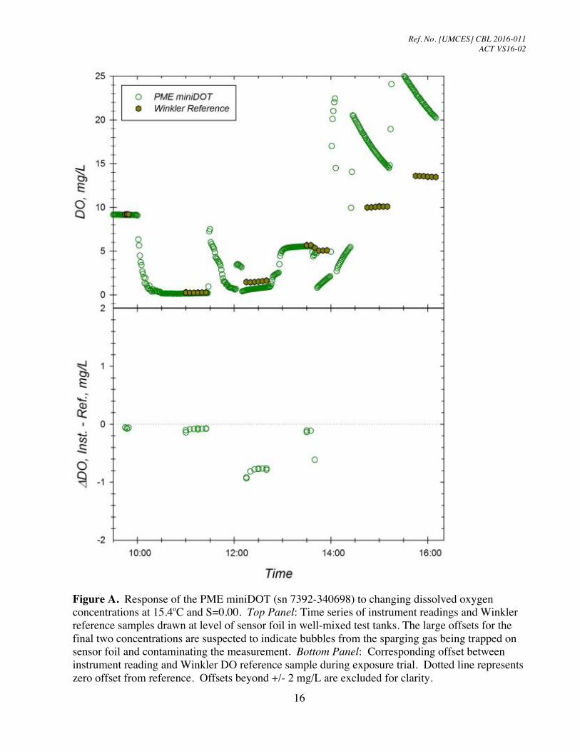
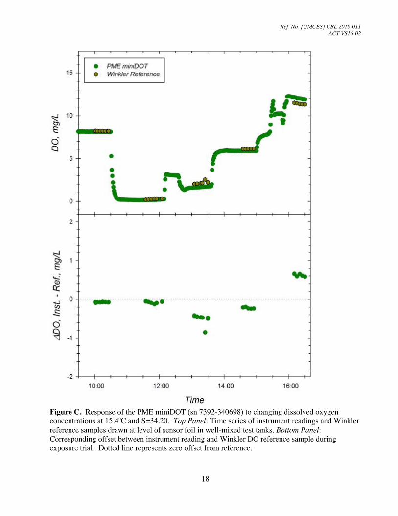
RESULTS of LABORATORY TESTING Instrument accuracy for the PME miniDOT sensor was tested under nine combinations of temperature and salinity over a range of DO concentrations from 10% to 120% of saturation. Specific test conditions are summarized in Table 1. Results are plotted as a time series of instrument readings against the time series of comparative Winkler reference samples (Figures A-I). The bottom panel of each figure shows the time series of the difference in instrument measurement versus corresponding reference sample. Plotted differences were limited to a range of ± 2.0 mg/L, as values exceeding this range are well outside any expected performance specification and likely occurred as a result of bubbles from the sparging gas used to vary dissolved oxygen concentrations getting trapped on the sensor foil. Comparisons of tank duplicates taken at opposite sides of the tank from between 9-18 of the timepoints during each trial showed a mean difference of 0.017 mg/L, with a range over the nine trials of 0.006 – 0.038 mg/L. Those values are within the analytical precision of the reference method and indicate conditions throughout the tank were very homogeneous and trapping of bubbles on the sensor foil happened as isolated events, which were clearly distinguishable. However, small changes in measured DO concentrations did occur during some of the sampling phases indicating the tank was slightly moderating after sparging was stopped. Those small drifts in DO concentrations were clearly captured by both instrument and reference sample measurements.

Ref. No. [UMCES] CBL 2016-011 ACT VS16-02
14
Table 1. Dissolved oxygen temperature and salinity challenge trial conditions. For each trial pre and post measurements of tank temperature (oC) and salinity (S) were made with an calibrated SBE26+4M CTD, equilibrated in well mixed tank for 20 min until stable readings obtained.
Trial ID Mean
Temperature oC
S.D. Temperature
oC
Mean Salinity
PSU
S.D. Salinity
PSU
Levels of DO tested
mg/L
Figure for
PME L_T15_S00 15.44 0.03 0.00 0.000 0, 2, 5,9,10,14 A L_T15_S10 15.47 0.01 8.82 0.003 0, 2, 8, 9, 13 B L_T15_S35 15.39 0.03 34.20 0.009 0,2,6,8,12 C L_T04_S00 5.40 0.08 0.00 0.000 0,4, 12, 17 D L_T04_S10 5.30 0.03 8.98 0.009 0, 5, 12, 16 E L_T04_S35 5.23 0.07 34.77 0.073 0, 4, 10, 14 F L_T30_S00 30.22 0.03 0.00 0.000 0, 3, 5, 9 G L_T30_S10 30.51 0.12 9.28 0.036 0, 3, 7, 10 H L_T30_S35 30.61 0.07 34.43 0.050 0, 2, 6, 9 I
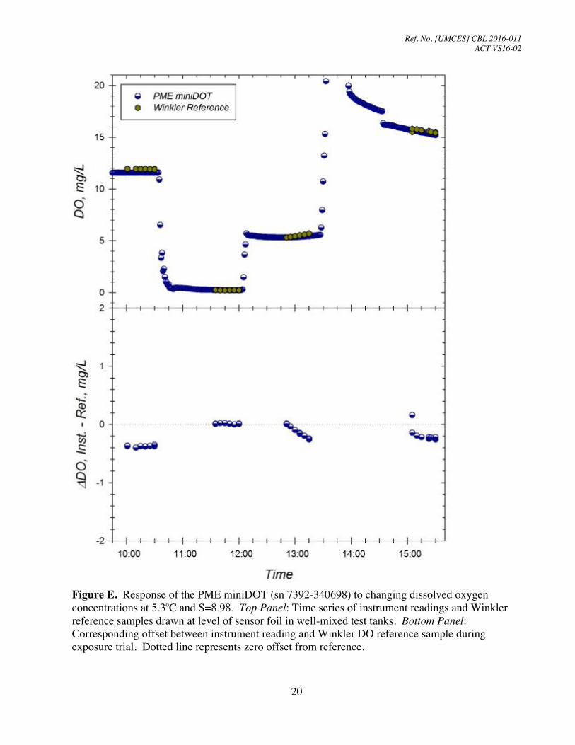
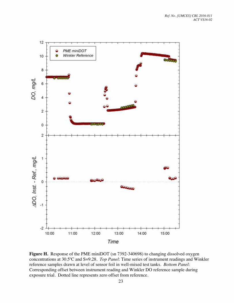
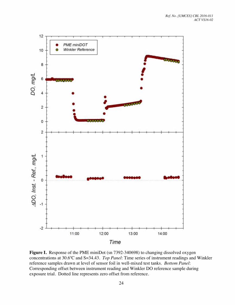
The mean and standard deviation of the differences between the PME miniDOT and reference measurements for each trial (n = 21 - 40) are presented in Table 2. Explanations for the difference between observed and possible comparative observations for the Lab trials are noted in the respective figure legends. Mean difference among trials ranged from -0.339 to 0.126 mg/L. There were no consistent trends in instrument accuracy across salinity ranges. There was a noticeable change in the direction of the offset across temperature ranges with the average offset equal to -0.23 mg/L for the 4 and 15 oC trials compared to a mean offset of 0.11 mg/L for the 30 oC trials. Table 2. Summary of the mean and standard deviation of offsets between paired PME miniDOT sensor measures and Winkler reference DO measures during laboratory trials.
Trial ID Instrument – Winkler DO
mean s.d. Observed n Possible n
L_T15_S00 -0.339 0.348 28 51 L_T15_S10 -0.291 0.268 21 39 L_T15_S35 -0.087 0.362 38 38 L_T04_S00 -0.201 0.119 39 39 L_T04_S10 -0.164 0.161 36 36 L_T04_S35 -0.336 0.223 37 37 L_T30_S00 0.126 0.081 40 40 L_T30_S10 0.080 0.240 39 39 L_T30_S35 0.109 0.030 40 40

Ref. No. [UMCES] CBL 2016-011 ACT VS16-02
15
The precision of the PME miniDOT sensor was also characterized for each of the nine
temperatures and salinity trials (Table 3). Precision trials were conducted at the start of each new tank test when conditions were most stable. Instruments were equilibrated in test tanks at indicated temperature and salinities for 45 min then the subsequent 31 one-minute measurements were used to estimate average tank DO (mg/L) and its variation over that interval. The absolute precision, estimated as the standard deviation (s.d.) around the mean, ranged from 0.005 – 0.013 mg/L across trials with an overall average of 0.008 mg/L. Relative precision, estimated as the coefficient of variation (CV% = (s.d./mean)x100), ranged from 0.057 – 0.248 percent across trials with an overall average of 0.098%. Table 3. Characterization of the precision of the PME miniDOT sensor over a range of temperatures and salinities test conditions.
Trial ID Temperature Salinity Dissolved Oxygen Reading mg/L mean mg/L s.d. CV% n
L_T15_S00 15.44 0.00 9.16 0.013 0.137 31 L_T15_S10 15.47 8.82 9.16 0.006 0.063 31 L_T15_S35 15.39 34.20 8.15 0.006 0.076 31 L_T04_S00 5.40 0.00 11.88 0.008 0.070 31 L_T04_S10 5.30 8.98 11.59 0.008 0.068 31 L_T04_S35 5.23 34.77 10.13 0.006 0.057 31 L_T30_S00 30.22 0.00 4.95 0.012 0.248 31 L_T30_S10 30.51 9.28 6.99 0.006 0.085 31 L_T30_S35 30.61 34.43 5.92 0.005 0.080 31
Ref. No. [UMCES] CBL 2016-011 ACT VS16-02
16
Figure A. Response of the PME miniDOT (sn 7392-340698) to changing dissolved oxygen concentrations at 15.4oC and S=0.00. Top Panel: Time series of instrument readings and Winkler reference samples drawn at level of sensor foil in well-mixed test tanks. The large offsets for the final two concentrations are suspected to indicate bubbles from the sparging gas being trapped on sensor foil and contaminating the measurement. Bottom Panel: Corresponding offset between instrument reading and Winkler DO reference sample during exposure trial. Dotted line represents zero offset from reference. Offsets beyond +/- 2 mg/L are excluded for clarity.

Ref. No. [UMCES] CBL 2016-011 ACT VS16-02
17
Figure B. Response of the PME miniDOT (sn 7392-340698) to changing dissolved oxygen concentrations at 15.4oC and S=8.82. Top Panel: Time series of instrument readings and Winkler reference samples drawn at level of sensor foil in well-mixed test tanks. The large offsets for the final two concentrations are suspected to indicate bubbles from the sparging gas being trapped on sensor foil and contaminating the measurement. Bottom Panel: Corresponding offset between instrument reading and Winkler DO reference sample during exposure trial. Dotted line represents zero offset from reference. Offsets beyond +/- 2 mg/L are excluded for clarity
Ref. No. [UMCES] CBL 2016-011 ACT VS16-02
18
Figure C. Response of the PME miniDOT (sn 7392-340698) to changing dissolved oxygen concentrations at 15.4oC and S=34.20. Top Panel: Time series of instrument readings and Winkler reference samples drawn at level of sensor foil in well-mixed test tanks. Bottom Panel: Corresponding offset between instrument reading and Winkler DO reference sample during exposure trial. Dotted line represents zero offset from reference.

Ref. No. [UMCES] CBL 2016-011 ACT VS16-02
19
Figure D. Response of the PME miniDOT (sn 7392-340698) to changing dissolved oxygen concentrations at 5.4oC and S=0.00. Top Panel: Time series of instrument readings and Winkler reference samples drawn at level of sensor foil in well-mixed test tanks. Bottom Panel: Corresponding offset between instrument reading and Winkler DO reference sample during exposure trial. Dotted line represents zero offset from reference.
Ref. No. [UMCES] CBL 2016-011 ACT VS16-02
20
Figure E. Response of the PME miniDOT (sn 7392-340698) to changing dissolved oxygen concentrations at 5.3oC and S=8.98. Top Panel: Time series of instrument readings and Winkler reference samples drawn at level of sensor foil in well-mixed test tanks. Bottom Panel: Corresponding offset between instrument reading and Winkler DO reference sample during exposure trial. Dotted line represents zero offset from reference.

Ref. No. [UMCES] CBL 2016-011 ACT VS16-02
21
Figure F. Response of the PME miniDOT (sn 7392-340698) to changing dissolved oxygen concentrations at 5.2oC and S=34.77. Top Panel: Time series of instrument readings and Winkler reference samples drawn at level of sensor foil in well-mixed test tanks. Bottom Panel: Corresponding offset between instrument reading and Winkler DO reference sample during exposure trial. Dotted line represents zero offset from reference.

Ref. No. [UMCES] CBL 2016-011 ACT VS16-02
22
Figure G. Response of the PME miniDOT (sn 7392-340698) to changing dissolved oxygen concentrations at 30.2oC and S=0.00. Top Panel: Time series of instrument readings and Winkler reference samples drawn at level of sensor foil in well-mixed test tanks. Bottom Panel: Corresponding offset between instrument reading and Winkler DO reference sample during exposure trial. Dotted line represents zero offset from reference.
Ref. No. [UMCES] CBL 2016-011 ACT VS16-02
23
Figure H. Response of the PME miniDOT (sn 7392-340698) to changing dissolved oxygen concentrations at 30.5oC and S=9.28. Top Panel: Time series of instrument readings and Winkler reference samples drawn at level of sensor foil in well-mixed test tanks. Bottom Panel: Corresponding offset between instrument reading and Winkler DO reference sample during exposure trial. Dotted line represents zero offset from reference.
Ref. No. [UMCES] CBL 2016-011 ACT VS16-02
24
Figure I. Response of the PME miniDot (sn 7392-340698) to changing dissolved oxygen concentrations at 30.6oC and S=34.43. Top Panel: Time series of instrument readings and Winkler reference samples drawn at level of sensor foil in well-mixed test tanks. Bottom Panel: Corresponding offset between instrument reading and Winkler DO reference sample during exposure trial. Dotted line represents zero offset from reference.
Ref. No. [UMCES] CBL 2016-011 ACT VS16-02
25
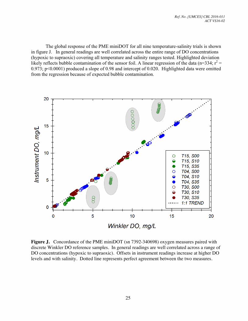
The global response of the PME miniDOT for all nine temperature-salinity trials is shown in figure J. In general readings are well correlated across the entire range of DO concentrations (hypoxic to supraoxic) covering all temperature and salinity ranges tested. Highlighted deviation likely reflects bubble contamination of the sensor foil. A linear regression of the data (n=334; r2 = 0.973; p<0.0001) produced a slope of 0.98 and intercept of 0.020. Highlighted data were omitted from the regression because of expected bubble contamination.
Figure J. Concordance of the PME miniDOT (sn 7392-340698) oxygen measures paired with discrete Winkler DO reference samples. In general readings are well correlated across a range of DO concentrations (hypoxic to supraoxic). Offsets in instrument readings increase at higher DO levels and with salinity. Dotted line represents perfect agreement between the two measures.
Ref. No. [UMCES] CBL 2016-011 ACT VS16-02
26
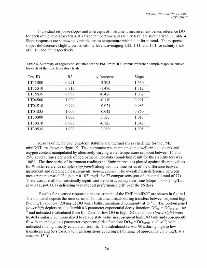
Individual response slopes and intercepts of instrument measurement versus reference DO for each of the laboratory trials at a fixed temperature and salinity level are summarized in Table 4. Slope responses are somewhat variable across temperature with no uniform trend. The response slopes did decrease slightly across salinity levels, averaging 1.22, 1.11, and 1.01 for salinity trials of 0, 10, and 35, respectively. Table 4. Summary of regression statistics for the PME miniDOT versus reference sample response curves for each of the nine laboratory trials. Test ID R2 y Intercept Slope LT15S00 0.921 -2.203 1.660 LT15S10 0.913 -1.470 1.312 LT15S35 0.996 -0.426 1.062 LT04S00 1.000 -0.110 0.991 LT04S10 0.999 -0.021 0.983 LT04S35 1.000 -0.042 0.960 LT30S00 1.000 0.053 1.018 LT30S10 0.997 -0.125 1.042 LT30S35 1.000 0.089 1.005
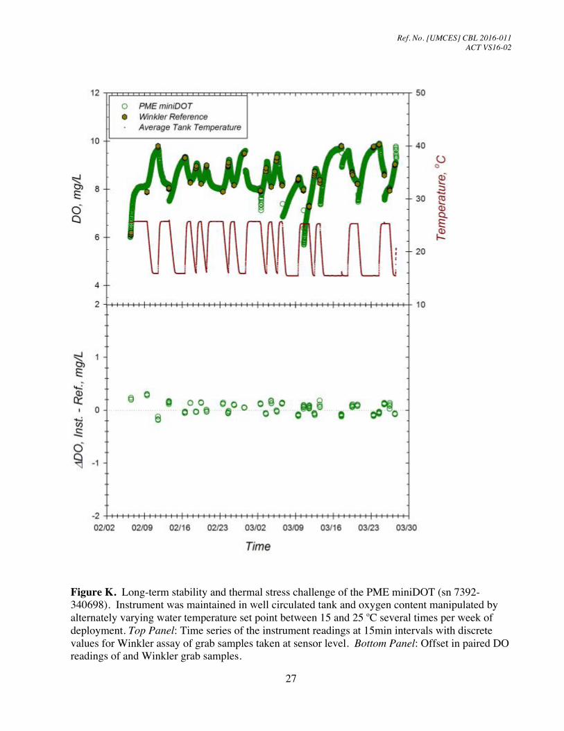
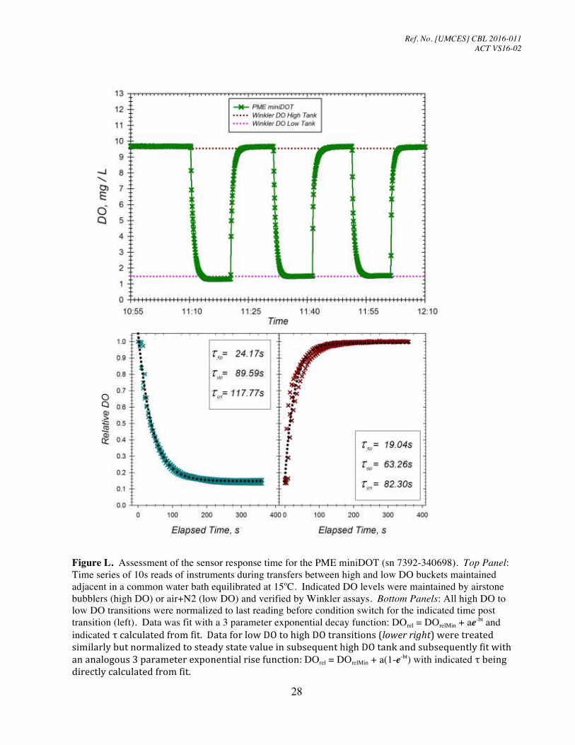
Results of the 56 day long-term stability and thermal stress challenge for the PME miniDOT are shown in figure K. The instrument was maintained in a well circulated tank and oxygen content manipulated by alternately varying water temperature set point between 15 and 25oC several times per week of deployment. The data completion result for the stability test was 100%. The time series of instrument readings at 15min intervals is plotted against discrete values for Winkler reference samples (top panel) along with the time series of the difference between instrument and reference measurements (bottom panel). The overall mean difference between measurements was 0.034 (s.d. = 0.107) mg/L for 77 comparisons (out of a potential total of 77). There was a small but statistically significant trend in accuracy over time (slope = -0.002 mg/L/d; r2 = 0.11; p=0.003) indicating very modest performance drift over the 56 days. Results for a sensor response time assessment of the PME miniDOT are shown in figure L. The top panel depicts the time series of 5s instrument reads during transfers between adjacent high (9.6 mg/L) and low (2.0 mg/L) DO water baths, maintained commonly at 15 oC. The bottom panel (lower left) depicts results fit with a 3 parameter exponential decay function: DOrel = DOrelMin + ae-
bt and indicated τ calculated from fit. Data for low DO to high DO transitions (lower right) were treated similarly but normalized to steady state value in subsequent high DO tank and subsequently fit with an analogous 3 parameter exponential rise function: DOrel = DOrelMin + a(1-e-bt) with indicated τ being directly calculated from fit. The calculated τ90 was 90 s during high to low transitions and 63 s for low to high transitions covering a DO range of approximately 8 mg/L at a constant 15 oC.
Ref. No. [UMCES] CBL 2016-011 ACT VS16-02
27
Figure K. Long-term stability and thermal stress challenge of the PME miniDOT (sn 7392-340698). Instrument was maintained in well circulated tank and oxygen content manipulated by alternately varying water temperature set point between 15 and 25 oC several times per week of deployment. Top Panel: Time series of the instrument readings at 15min intervals with discrete values for Winkler assay of grab samples taken at sensor level. Bottom Panel: Offset in paired DO readings of and Winkler grab samples.
Ref. No. [UMCES] CBL 2016-011 ACT VS16-02
28
Figure L. Assessment of the sensor response time for the PME miniDOT (sn 7392-340698). Top Panel: Time series of 10s reads of instruments during transfers between high and low DO buckets maintained adjacent in a common water bath equilibrated at 15oC. Indicated DO levels were maintained by airstone bubblers (high DO) or air+N2 (low DO) and verified by Winkler assays. Bottom Panels: All high DO to low DO transitions were normalized to last reading before condition switch for the indicated time post transition (left). Data was fit with a 3 parameter exponential decay function: DOrel = DOrelMin + ae-bt and indicated τcalculatedfromfit.DataforlowDOtohighDOtransitions(lowerright)weretreatedsimilarlybutnormalizedtosteadystatevalueinsubsequenthighDOtankandsubsequentlyfitwithananalogous3parameterexponentialrisefunction:DOrel = DOrelMin + a(1-e-bt) with indicated τbeingdirectlycalculatedfromfit.
Ref. No. [UMCES] CBL 2016-011 ACT VS16-02
29
RESULTS of MOORED FIELD TESTS Moored field tests were conducted to examine the performance of the PME miniDOT to
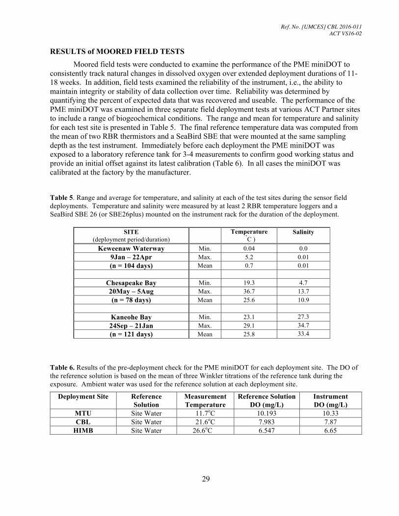
consistently track natural changes in dissolved oxygen over extended deployment durations of 11-18 weeks. In addition, field tests examined the reliability of the instrument, i.e., the ability to maintain integrity or stability of data collection over time. Reliability was determined by quantifying the percent of expected data that was recovered and useable. The performance of the PME miniDOT was examined in three separate field deployment tests at various ACT Partner sites to include a range of biogeochemical conditions. The range and mean for temperature and salinity for each test site is presented in Table 5. The final reference temperature data was computed from the mean of two RBR thermistors and a SeaBird SBE that were mounted at the same sampling depth as the test instrument. Immediately before each deployment the PME miniDOT was exposed to a laboratory reference tank for 3-4 measurements to confirm good working status and provide an initial offset against its latest calibration (Table 6). In all cases the miniDOT was calibrated at the factory by the manufacturer.
Table 5. Range and average for temperature, and salinity at each of the test sites during the sensor field deployments. Temperature and salinity were measured by at least 2 RBR temperature loggers and a SeaBird SBE 26 (or SBE26plus) mounted on the instrument rack for the duration of the deployment.
SITE (deployment period/duration) Temperature
°C ) Salinity
Keweenaw Waterway Min. 0.04 0.0
9Jan – 22Apr Max. 5.2 0.01 (n = 104 days) Mean 0.7 0.01
Chesapeake Bay Min. 19.3 4.7 20May – 5Aug Max. 36.7 13.7 (n = 78 days) Mean 25.6 10.9
Kaneohe Bay Min. 23.1 27.3 24Sep – 21Jan Max. 29.1 34.7 (n = 121 days) Mean 25.8 33.4
Table 6. Results of the pre-deployment check for the PME miniDOT for each deployment site. The DO of the reference solution is based on the mean of three Winkler titrations of the reference tank during the exposure. Ambient water was used for the reference solution at each deployment site.
Deployment Site Reference Solution
Measurement Temperature
Reference Solution DO (mg/L)
Instrument DO (mg/L)
MTU Site Water 11.7oC 10.193 10.33 CBL Site Water 21.6oC 7.983 7.87
HIMB Site Water 26.6oC 6.547 6.65

Ref. No. [UMCES] CBL 2016-011 ACT VS16-02
30
Michigan Tech Great Lakes Research Center Field Deployment Site A 15 week deployment under ice took place from January 9 through April 22 in the Keweenaw
Waterway adjacent to the Great Lakes Research Center in Houghton, MI. The deployment site was located at 47.12° N, 88.55° W, at the end of the pier at the Great Lakes Research Center docks. This site is located on the south side of the Keweenaw Waterway, and is connected to Lake Superior in both the NW and SE directions. The instrumentation rack was lowered off of the end of the pier with a ½ ton crane and rested on the bottom, under the ice, in 4.5m of water. A small shelter was constructed at the end of the pier to provide shelter for processing the reference samples during winter sampling efforts.
Photo 1. Aerial view of the Keweenaw Waterway (left) and dockside mooring deployment (right).
Time series results of ambient conditions for temperature and specific conductivity are given in figure 1. Temperature ranged from 0.04 - 5.3oC and specific conductivity from 49 - 110 µS/cm over the duration of the field test. The bottom panel displays the maximum difference recorded between all reference thermistors mounted at the same depth as the sensors sampling intakes as well as a meter above, at different locations across the mooring rack. The average temperature difference observed across the space of the mooring rack was 0.01°C with a maximum of 0.98oC. Differences between instrument and reference readings resulting from this variability should be minimized as the sampling bottle integrates across the mooring space.
Unexpected shifts between adjacent reference samples were noted on three occasions
during the test. Upon inspection it was determined that these excursions occurred during changes in the batches of Winkler reagents. A correction to reference values was subsequently made based on the magnitude of change observed between the adjacent Winkler measurements after adjusting for ambient changes determined by the average of all seven DO sensors deployed on the mooring. Adjusted values are noted within each figure.
The PME miniDOT operated successfully throughout the entire 15week deployment and
generated 9,859 observations based on its 15 minute sampling interval for a data completion result of 100%. It should be noted that for this deployment a wiping system was not yet available, so some caution should be used in comparisons against the other field test results. Time series results of the PME and corresponding reference DO results are given in figure 2 (top panel). Ambient DO
Ref. No. [UMCES] CBL 2016-011 ACT VS16-02
31
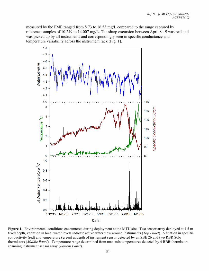
measured by the PME ranged from 8.73 to 16.53 mg/L compared to the range captured by reference samples of 10.249 to 14.007 mg/L. The sharp excursion between April 8 - 9 was real and was picked up by all instruments and correspondingly seen in specific conductance and temperature variability across the instrument rack (Fig. 1).
Figure 1. Environmental conditions encountered during deployment at the MTU site. Test sensor array deployed at 4.5 m fixed depth, variation in local water levels indicate active water flow around instruments (Top Panel). Variation in specific conductivity (red) and temperature (green) at depth of instrument sensor detected by an SBE 26 and two RBR Solo thermistors (Middle Panel). Temperature range determined from max-min temperatures detected by 4 RBR thermistors spanning instrument sensor array (Bottom Panel).

Ref. No. [UMCES] CBL 2016-011 ACT VS16-02
32
The time series of the difference between instrument and reference DO measurements for each matched pair (n=118 observations) is given in the bottom panel of figure 2. The average and standard deviation of the measurement difference over the total deployment was 0.029 ± 0.072 mg/L with a total range of -0.307 to 0.205mg/L. The drift rate of instrument offset, estimated by linear regression (r2=0.373; p<0.0001), was 0.001 mg/L/d. This rate would include any biofouling effects as well as any electronic or calibration drift.
Figure 2. Time series of DO measured detected by PME miniDOT deployed during the 15 week Great Lakes field trial. Top Panel: Continuous DO recordings from instrument (blue line) and DO of adjacent grab samples determined by Winkler titration (red circles and yellow circles for adjusted Winkler results due to corrections across reagent batches). Bottom Panel: Difference in measured DO relative to reference samples (Instrument DO mg/L – Reference DO mg/L) observed during deployment. Insert: Close up of excursion that occurred 4/8-4/9. No reference samples were collected during this time period.
Ref. No. [UMCES] CBL 2016-011 ACT VS16-02
33
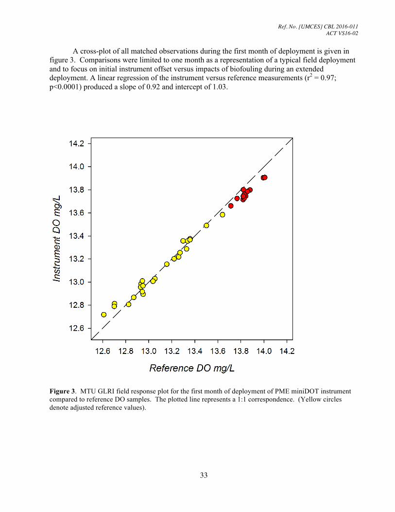
A cross-plot of all matched observations during the first month of deployment is given in figure 3. Comparisons were limited to one month as a representation of a typical field deployment and to focus on initial instrument offset versus impacts of biofouling during an extended deployment. A linear regression of the instrument versus reference measurements (r2 = 0.97; p<0.0001) produced a slope of 0.92 and intercept of 1.03.
Figure 3. MTU GLRI field response plot for the first month of deployment of PME miniDOT instrument compared to reference DO samples. The plotted line represents a 1:1 correspondence. (Yellow circles denote adjusted reference values).

Ref. No. [UMCES] CBL 2016-011 ACT VS16-02
34
Photos of test instrument before and after the field deployment to indicate potential impact of biofouling (Photo 2).
Photo 2. PME miniDOT prior to and following 15 week deployment under ice for the MTU field test.
Ref. No. [UMCES] CBL 2016-011 ACT VS16-02
35
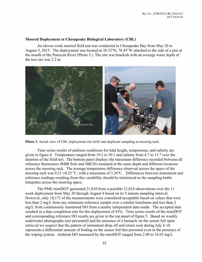
Moored Deployment at Chesapeake Biological Laboratory (CBL) An eleven week moored field test was conducted in Chesapeake Bay from May 20 to
August 5, 2015. The deployment was located at 38.32°N, 76.45°W attached to the side of a pier at the mouth of the Patuxent River (Photo 3.) The site was brackish with an average water depth of the test site was 2.2 m.
Photo 3. Aerial view of CBL deployment site (left) and duplicate sampling at mooring rack.
Time series results of ambient conditions for tidal height, temperature, and salinity are given in figure 4. Temperature ranged from 19.2 to 30.1 and salinity from 4.7 to 13.7 over the duration of the field test. The bottom panel displays the maximum difference recorded between all reference thermistors (RBR Solo and SBE26) mounted at the same depth and different locations across the mooring rack. The average temperature difference observed across the space of the mooring rack was 0.21 ±0.25 oC, with a maximum of 3.26oC. Differences between instrument and reference readings resulting from this variability should be minimized as the sampling bottle integrates across the mooring space.
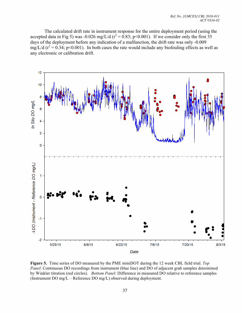
The PME miniDOT generated 21,810 from a possible 21,810 observations over the 11 week deployment from May 20 through August 4 based on its 5 minute sampling interval. However, only 18,173 of the measurements were considered acceptable based on values that were less than 2 mg/L from any minimum reference sample over a similar timeframe and less than 2 mg/L from continuously monitored DO from a nearby independent data sonde. The accepted data resulted in a data completion rate for this deployment of 83%. Time series results of the miniDOT and corresponding reference DO results are given in the top panel of figure 5. Based on weekly underwater photographs (not presented) and the presence of a barnacle on the sensor foil upon retrieval we suspect that the pattern of instrument drop off and return seen during July 6-18 represents a differential amount of fouling on the sensor foil that persisted even in the presence of the wiping system. Ambient DO measured by the miniDOT ranged from 2.00 to 10.65 mg/L

Ref. No. [UMCES] CBL 2016-011 ACT VS16-02
36
compared to the range captured by the reference measurements of 4.370 to 10.85 mg/L. The bottom panel presents the time series of the difference between the miniDOT and reference DO for each matched pair (limited to ±2.0 mg/L; n=109 observations out of a total of 142). The average and standard deviation of the measurement difference for the deployment was -0.40 ±0.702 mg/L, with the total range of differences between -1.90 to 0.86 mg/L.
Figure 4. Environmental conditions encountered during the 11 week CBL floating dock deployment. Test
sensor array deployed at 1 m fixed depth, variation in local tidal heights indicate active water flow around instrument (Top Panel). Variation in salinity (red) and temperature (green) at depth of instrument sensor detected by an SBE 26 and two RBR Solo thermistors (Middle Panel). Temperature range determined from max-min temperatures detected by RBR thermistors spanning instrument sensor array (Bottom Panel).
Ref. No. [UMCES] CBL 2016-011 ACT VS16-02
37
The calculated drift rate in instrument response for the entire deployment period (using the accepted data in Fig 5) was -0.026 mg/L/d (r2 = 0.83; p<0.001). If we consider only the first 35 days of the deployment before any indication of a malfunction, the drift rate was only -0.009 mg/L/d (r2 = 0.34; p<0.001). In both cases the rate would include any biofouling effects as well as any electronic or calibration drift.
Figure 5. Time series of DO measured by the PME miniDOT during the 12 week CBL field trial. Top Panel: Continuous DO recordings from instrument (blue line) and DO of adjacent grab samples determined by Winkler titration (red circles). Bottom Panel: Difference in measured DO relative to reference samples (Instrument DO mg/L – Reference DO mg/L) observed during deployment.

Ref. No. [UMCES] CBL 2016-011 ACT VS16-02
38
A cross-plot of all matched observations for the first month of the deployment is given in figure 6. Comparisons were limited to one month as a representation of a typical field deployment and to focus on initial instrument offset versus impacts of biofouling during an extended deployment. A linear regression of the instrument versus reference measurements (r2 = 0.98; p<0.001) produced a slope of 0.968 and intercept of 0.306.
Figure 6. CBL field response plot for PME miniDOT compared to reference DO samples. The plotted line represents a 1:1 correspondence.
Ref. No. [UMCES] CBL 2016-011 ACT VS16-02
39
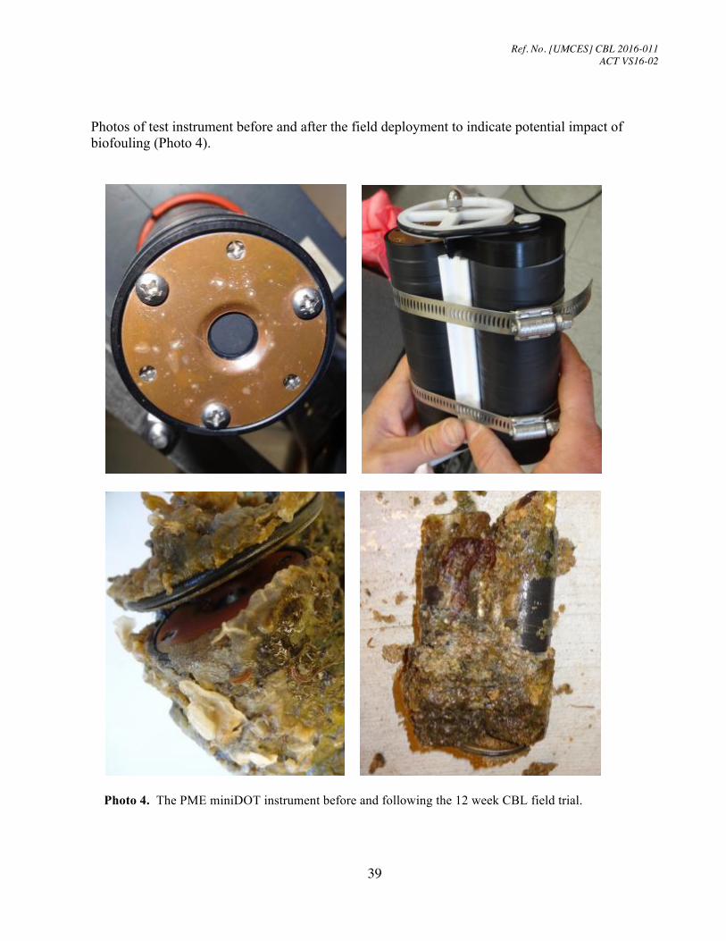
Photos of test instrument before and after the field deployment to indicate potential impact of biofouling (Photo 4).
Photo 4. The PME miniDOT instrument before and following the 12 week CBL field trial.
Ref. No. [UMCES] CBL 2016-011 ACT VS16-02
40
Moored Deployment off Coconut Island in Kaneohe Bay, Hawaii
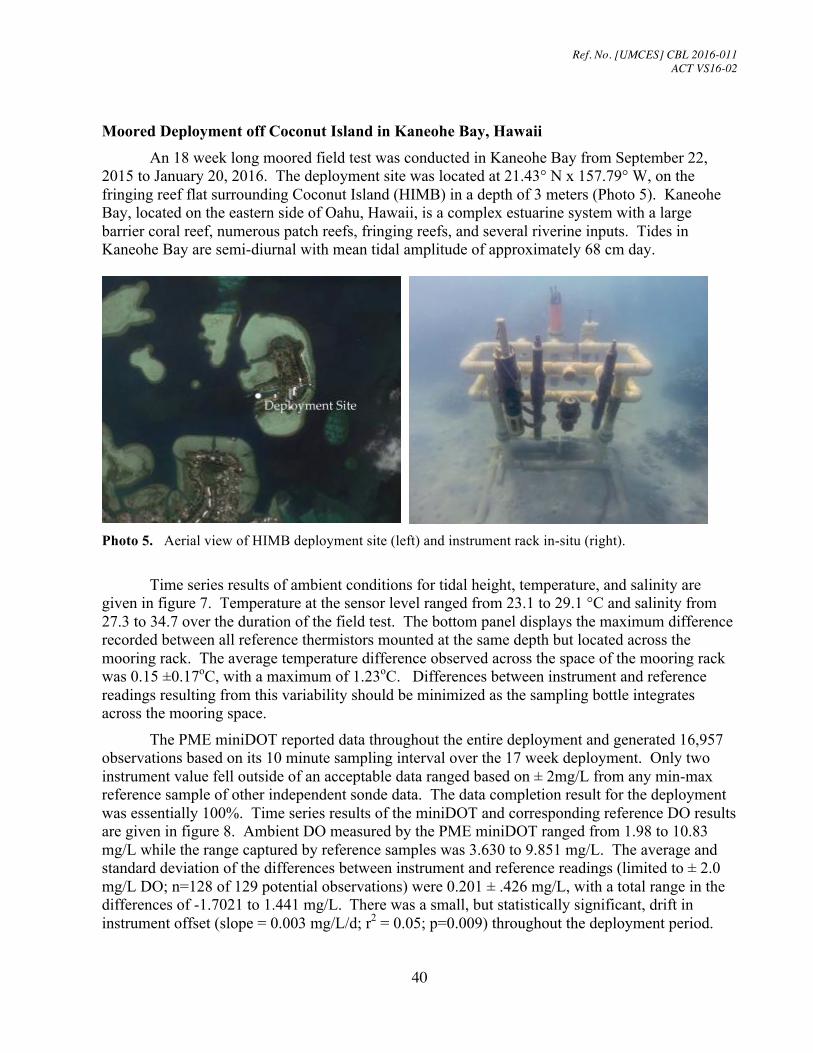
An 18 week long moored field test was conducted in Kaneohe Bay from September 22, 2015 to January 20, 2016. The deployment site was located at 21.43° N x 157.79° W, on the fringing reef flat surrounding Coconut Island (HIMB) in a depth of 3 meters (Photo 5). Kaneohe Bay, located on the eastern side of Oahu, Hawaii, is a complex estuarine system with a large barrier coral reef, numerous patch reefs, fringing reefs, and several riverine inputs. Tides in Kaneohe Bay are semi-diurnal with mean tidal amplitude of approximately 68 cm day.
Photo 5. Aerial view of HIMB deployment site (left) and instrument rack in-situ (right).
Time series results of ambient conditions for tidal height, temperature, and salinity are given in figure 7. Temperature at the sensor level ranged from 23.1 to 29.1 °C and salinity from 27.3 to 34.7 over the duration of the field test. The bottom panel displays the maximum difference recorded between all reference thermistors mounted at the same depth but located across the mooring rack. The average temperature difference observed across the space of the mooring rack was 0.15 ±0.17oC, with a maximum of 1.23oC. Differences between instrument and reference readings resulting from this variability should be minimized as the sampling bottle integrates across the mooring space.
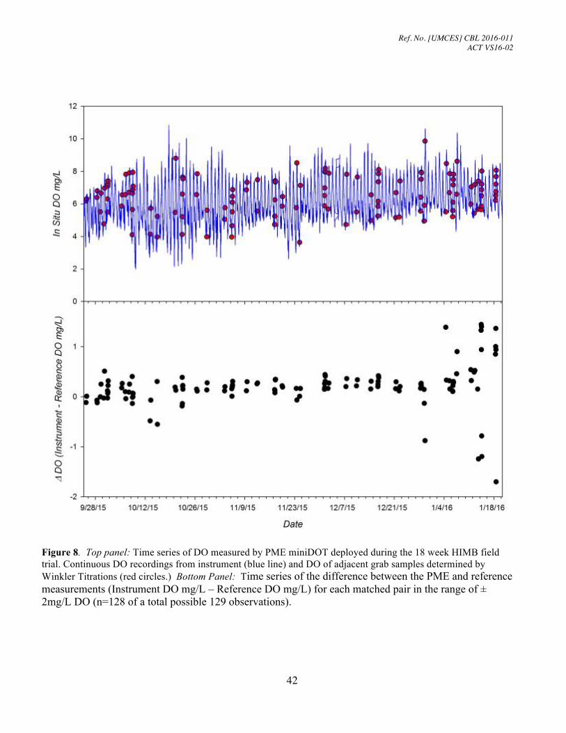
The PME miniDOT reported data throughout the entire deployment and generated 16,957 observations based on its 10 minute sampling interval over the 17 week deployment. Only two instrument value fell outside of an acceptable data ranged based on ± 2mg/L from any min-max reference sample of other independent sonde data. The data completion result for the deployment was essentially 100%. Time series results of the miniDOT and corresponding reference DO results are given in figure 8. Ambient DO measured by the PME miniDOT ranged from 1.98 to 10.83 mg/L while the range captured by reference samples was 3.630 to 9.851 mg/L. The average and standard deviation of the differences between instrument and reference readings (limited to ± 2.0 mg/L DO; n=128 of 129 potential observations) were 0.201 ± .426 mg/L, with a total range in the differences of -1.7021 to 1.441 mg/L. There was a small, but statistically significant, drift in instrument offset (slope = 0.003 mg/L/d; r2 = 0.05; p=0.009) throughout the deployment period.

Ref. No. [UMCES] CBL 2016-011 ACT VS16-02
41
The scatter near the end of the deployment resulted in a very low goodness of fit in the regression. This rate would include any biofouling effects as well as any electronic or calibration drift.
Figure 7. Environmental conditions encountered during the 4 month HIMB deployment on the fringing reef flat off Coconut Island Test sensor array deployed at 1 m fixed depth, variation in local tidal heights indicate active water flow around instrument (Top Panel). Variation in salinity (red) and temperature (green) at depth of instrument sensor detected by an SBE 26 and two RBR Solo thermistors (Middle Panel). Temperature range determined from max-min temperatures detected by RBR thermistors spanning instrument sensor array (Bottom Panel).
Ref. No. [UMCES] CBL 2016-011 ACT VS16-02
42
Figure 8. Top panel: Time series of DO measured by PME miniDOT deployed during the 18 week HIMB field trial. Continuous DO recordings from instrument (blue line) and DO of adjacent grab samples determined by Winkler Titrations (red circles.) Bottom Panel: Time series of the difference between the PME and reference measurements (Instrument DO mg/L – Reference DO mg/L) for each matched pair in the range of ± 2mg/L DO (n=128 of a total possible 129 observations).
Ref. No. [UMCES] CBL 2016-011 ACT VS16-02
43
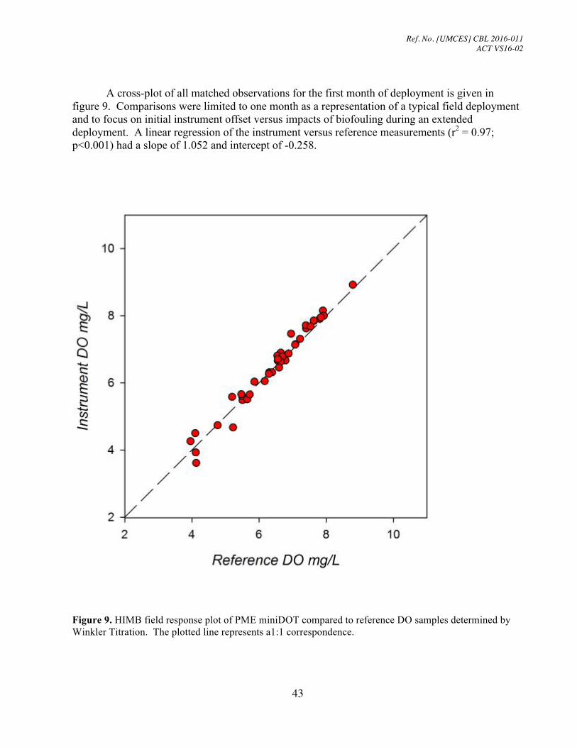
A cross-plot of all matched observations for the first month of deployment is given in figure 9. Comparisons were limited to one month as a representation of a typical field deployment and to focus on initial instrument offset versus impacts of biofouling during an extended deployment. A linear regression of the instrument versus reference measurements (r2 = 0.97; p<0.001) had a slope of 1.052 and intercept of -0.258.
Figure 9. HIMB field response plot of PME miniDOT compared to reference DO samples determined by Winkler Titration. The plotted line represents a1:1 correspondence.
Ref. No. [UMCES] CBL 2016-011 ACT VS16-02
44
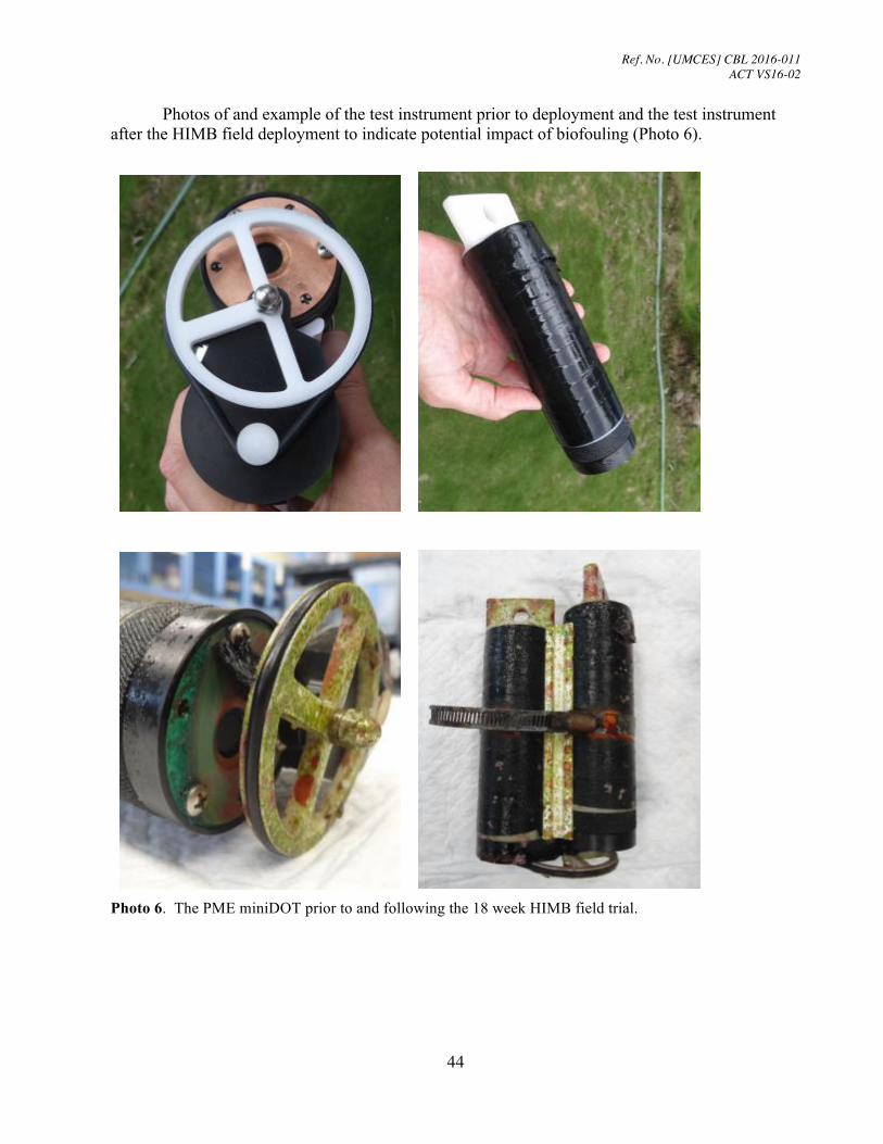
Photos of and example of the test instrument prior to deployment and the test instrument after the HIMB field deployment to indicate potential impact of biofouling (Photo 6).
Photo 6. The PME miniDOT prior to and following the 18 week HIMB field trial.
Ref. No. [UMCES] CBL 2016-011 ACT VS16-02
45
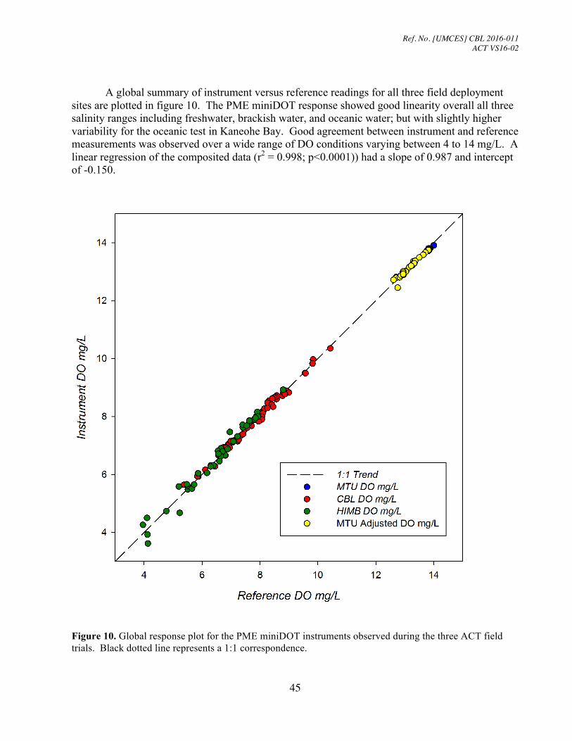
A global summary of instrument versus reference readings for all three field deployment
sites are plotted in figure 10. The PME miniDOT response showed good linearity overall all three salinity ranges including freshwater, brackish water, and oceanic water; but with slightly higher variability for the oceanic test in Kaneohe Bay. Good agreement between instrument and reference measurements was observed over a wide range of DO conditions varying between 4 to 14 mg/L. A linear regression of the composited data (r2 = 0.998; p<0.0001)) had a slope of 0.987 and intercept of -0.150.
Figure 10. Global response plot for the PME miniDOT instruments observed during the three ACT field trials. Black dotted line represents a 1:1 correspondence.
Ref. No. [UMCES] CBL 2016-011 ACT VS16-02
46
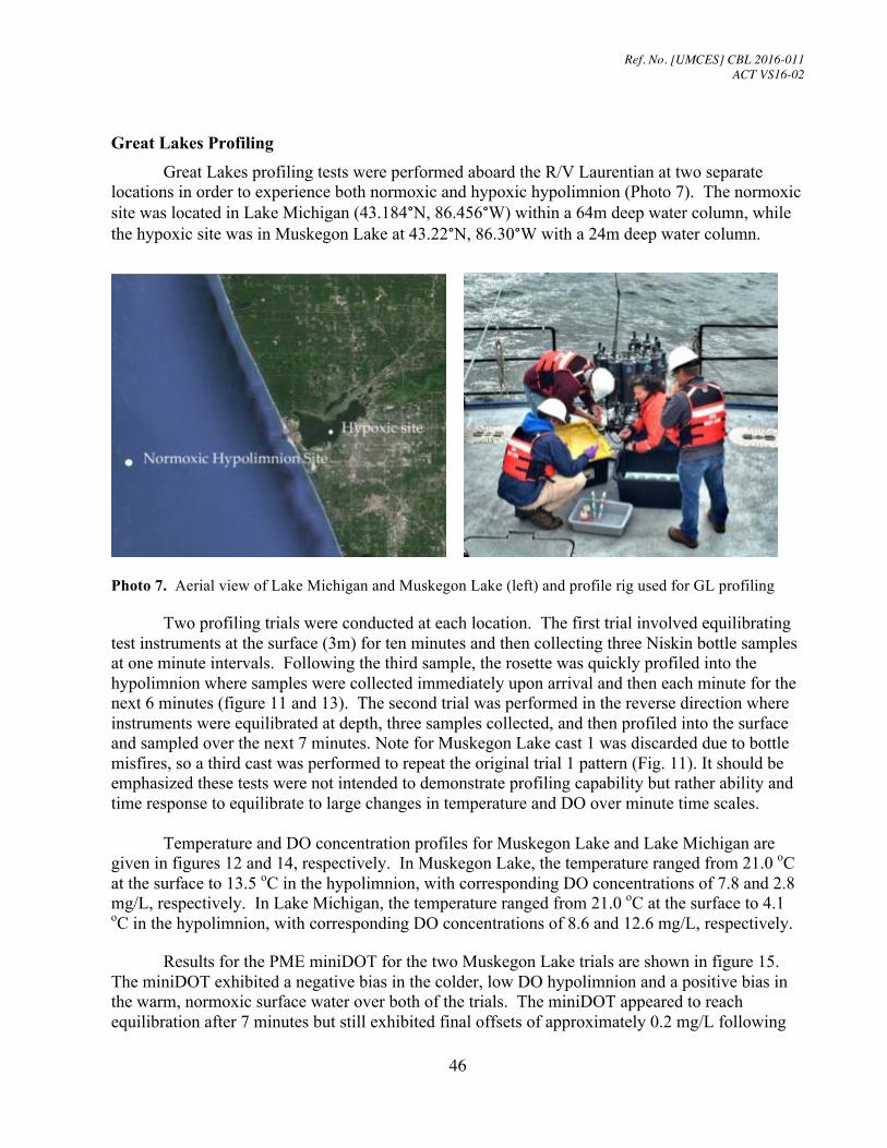
Great Lakes Profiling
Great Lakes profiling tests were performed aboard the R/V Laurentian at two separate locations in order to experience both normoxic and hypoxic hypolimnion (Photo 7). The normoxic site was located in Lake Michigan (43.184°N, 86.456°W) within a 64m deep water column, while the hypoxic site was in Muskegon Lake at 43.22°N, 86.30°W with a 24m deep water column.
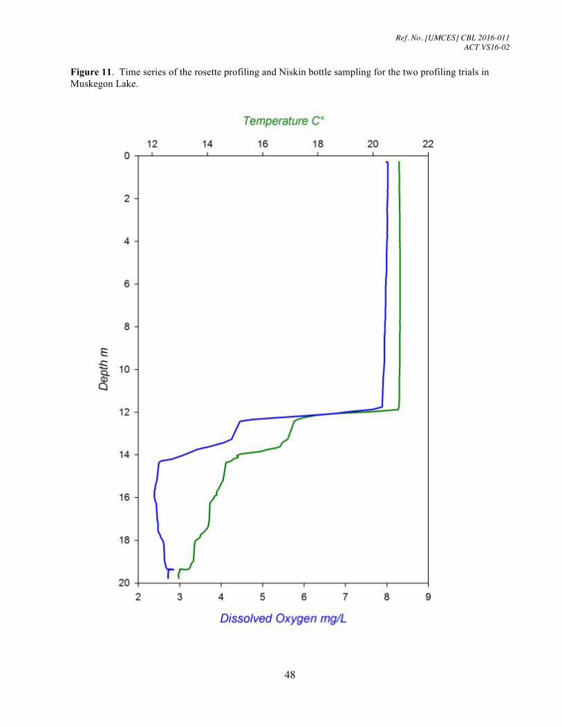
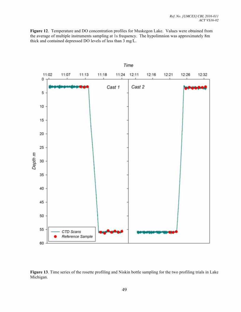
Photo 7. Aerial view of Lake Michigan and Muskegon Lake (left) and profile rig used for GL profiling Two profiling trials were conducted at each location. The first trial involved equilibrating test instruments at the surface (3m) for ten minutes and then collecting three Niskin bottle samples at one minute intervals. Following the third sample, the rosette was quickly profiled into the hypolimnion where samples were collected immediately upon arrival and then each minute for the next 6 minutes (figure 11 and 13). The second trial was performed in the reverse direction where instruments were equilibrated at depth, three samples collected, and then profiled into the surface and sampled over the next 7 minutes. Note for Muskegon Lake cast 1 was discarded due to bottle misfires, so a third cast was performed to repeat the original trial 1 pattern (Fig. 11). It should be emphasized these tests were not intended to demonstrate profiling capability but rather ability and time response to equilibrate to large changes in temperature and DO over minute time scales. Temperature and DO concentration profiles for Muskegon Lake and Lake Michigan are given in figures 12 and 14, respectively. In Muskegon Lake, the temperature ranged from 21.0 oC at the surface to 13.5 oC in the hypolimnion, with corresponding DO concentrations of 7.8 and 2.8 mg/L, respectively. In Lake Michigan, the temperature ranged from 21.0 oC at the surface to 4.1 oC in the hypolimnion, with corresponding DO concentrations of 8.6 and 12.6 mg/L, respectively. Results for the PME miniDOT for the two Muskegon Lake trials are shown in figure 15. The miniDOT exhibited a negative bias in the colder, low DO hypolimnion and a positive bias in the warm, normoxic surface water over both of the trials. The miniDOT appeared to reach equilibration after 7 minutes but still exhibited final offsets of approximately 0.2 mg/L following
Ref. No. [UMCES] CBL 2016-011 ACT VS16-02
47
the profiled transitions. The range in measurement differences between instrument and reference was -0.24 to 0.75 mg/L for cast 2 and -0.57 to 0.14 mg/L for cast 3. Results for the PME miniDOT for the two Lake Michigan trials are shown in figure 16. The miniDOT was well match during surface equilibration and then exhibited a strong negative bias when rapidly transitioned to the cold high DO hypolimnion. The sensor did not fully equilibrate after 7 minutes and ended at -0.8 mg/L against the reference. For cast 2, there was a negative offset of -0.6 mg/L when equilibrated in the hypolimnion and a positive bias when rapidly transitioned into the warm normoxic surface. The sensor appeared to reach equilibration after 7 minutes but with a final offset of around 0.4 mg/L against the reference. The range in measurement differences between instrument and reference was -2.03 to 0.03 mg/L for cast 1 and -0.72 to 1.63 mg/L for cast 2.
Ref. No. [UMCES] CBL 2016-011 ACT VS16-02
48
Figure 11. Time series of the rosette profiling and Niskin bottle sampling for the two profiling trials in Muskegon Lake.
Ref. No. [UMCES] CBL 2016-011 ACT VS16-02
49
Figure 12. Temperature and DO concentration profiles for Muskegon Lake. Values were obtained from the average of multiple instruments sampling at 1s frequency. The hypolimnion was approximately 8m thick and contained depressed DO levels of less than 3 mg/L.
Figure 13. Time series of the rosette profiling and Niskin bottle sampling for the two profiling trials in Lake Michigan.
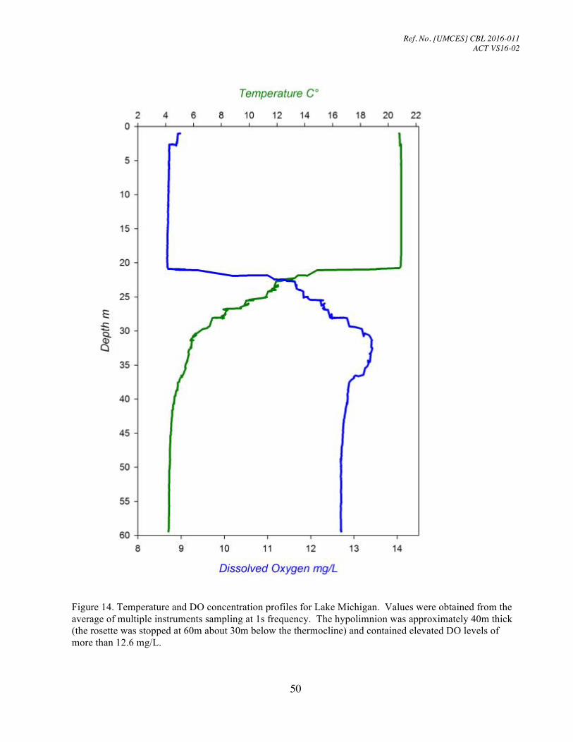
Ref. No. [UMCES] CBL 2016-011 ACT VS16-02
50
Figure 14. Temperature and DO concentration profiles for Lake Michigan. Values were obtained from the average of multiple instruments sampling at 1s frequency. The hypolimnion was approximately 40m thick (the rosette was stopped at 60m about 30m below the thermocline) and contained elevated DO levels of more than 12.6 mg/L.

Ref. No. [UMCES] CBL 2016-011 ACT VS16-02
51
Figure 15. Results of the PME miniDOT for the Muskegon Lake trials. Top panel: PME temperature data at sample snap. Middle panel: DO recordings from instrument (blue dot) and DO of corresponding reference samples determined by Winkler Titrations (red triangles.) Bottom panel: Time series of the difference between the PME and reference measurements for each matched pair. Cast 2 and 3 are plotted on the same graph and separated by the axis break. Bottle 8 on cast 3 did not close fully and was discarded.
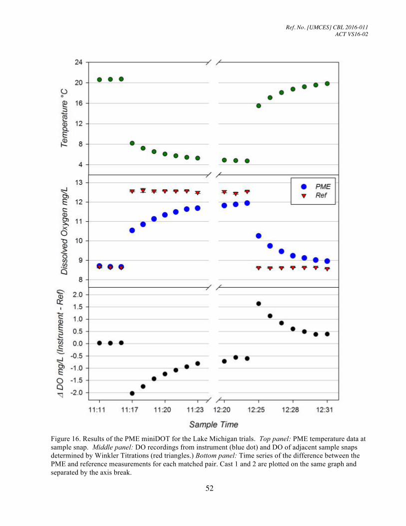
Ref. No. [UMCES] CBL 2016-011 ACT VS16-02
52
Figure 16. Results of the PME miniDOT for the Lake Michigan trials. Top panel: PME temperature data at sample snap. Middle panel: DO recordings from instrument (blue dot) and DO of adjacent sample snaps determined by Winkler Titrations (red triangles.) Bottom panel: Time series of the difference between the PME and reference measurements for each matched pair. Cast 1 and 2 are plotted on the same graph and separated by the axis break.

Ref. No. [UMCES] CBL 2016-011 ACT VS16-02
53
QUALITY ASSURANCE AND QUALITY CONTROL All technical activities conducted by ACT comply with ACT’s Quality Management System
(QMS), which includes the policies, objectives, procedures, authority, and accountability needed to ensure quality in ACT’s work processes, products, and services. The QMS provides the framework for quality assurance (QA) functions, which cover planning, implementation, and review of data collection activities and the use of data in decision making, and quality control. The QMS also ensures that all ACT data collection and processing activities are carried out in a consistent manner, to produce data of known and documented quality that can be used with a high degree of certainty by the intended user to support specific decisions or actions regarding technology performance. ACT’s QMS meets the requirements of ISO/IEC 17025:2005(E), General requirements for the competence of testing and calibration laboratories; the American National Standards Institute (ANSI)/American Society for Quality (ASQ) E4-2004 Quality Systems for Environmental Data and Technology Programs; and U.S. Environmental Protection Agency, quality standards for environmental data collection, production, and use. An effective assessment program is an integral part of ACT’s quality system. The ACT Quality Assurance (QA) Manager independently conducted two Technical Systems Audits (TSA) and data quality assessments of the reference sample data for the DO verification.
Quality Control Samples
Each site conducted weekly field duplicates which are presented below in Tables 7 – 9. The global average of the standard deviation among field duplicates for all field test sites was 0.03 ±0.07 (n=27), with 11 values exceeding our expected quality threshold of better than 0.013 mg/L DO. The average of the standard deviation among MTU field duplicates was .011 ±.014 (n=12), the average for CBL was .074 ±.006 (n=9) and the average for HIMB was .011 ±.012 (n=6). The higher variability at CBL likely reflected fine-scale heterogeneity in the water mass as was also noted by the greater variation in temperature across the mooring rack. In general, results attest to the representativeness of our sampling to water mass being analyzed by the test instruments and to consistent sample handling.
Table 7. Results of Field Duplicates (FD) for the Keweenaw Waterway, MI mooring test. Date/Time Rep Temp Spec
Cond DO Std
Dev Mean Std
Dev ABS Diff
1-14-15 10:30 FD1 .06 94 13.819 .005 13.819 0.00 0.000 FD2 13.819 .002
1-22-15 12:30 FD1 .31 99 12.981 .013 12.986 .007 .010 FD2 12.991 .005
1-29-15 16:00 FD1 .24 103 12.958 .041 12.947 .015 .021 FD2 12.937 .013
2-5-15 15:30 FD1 .21 106 12.671 .004 12.667 .006 .009 FD2 12.662 .007
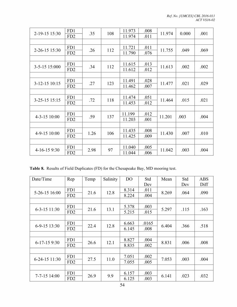
Ref. No. [UMCES] CBL 2016-011 ACT VS16-02
54
2-19-15 15:30 FD1 .35 108 11.973 .008 11.974 0.000 .001 FD2 11.974 .011
2-26-15 15:30 FD1 .26 112 11.721 .011 11.755 .049 .069 FD2 11.790 .076
3-5-15 15:000 FD1 .34 112 11.615 .013 11.613 .002 .002 FD2 11.612 .012
3-12-15 10:15 FD1 .27 123 11.491 .028 11.477 .021 .029 FD2 11.462 .007
3-25-15 15:15 FD1 .72 118 11.474 .051 11.464 .015 .021 FD2 11.453 .012
4-3-15 10:00 FD1 .59 137 11.199 .012 11.201 .003 .004 FD2 11.203 .001
4-9-15 10:00 FD1 1.26 106 11.435 .008 11.430 .007 .010 FD2 11.425 .009
4-16-15 9:30 FD1 2.98 97 11.040 .005 11.042 .003 .004 FD2 11.044 .006
Table 8. Results of Field Duplicates (FD) for the Chesapeake Bay, MD mooring test. Date/Time Rep Temp Salinity DO Std
Dev Mean Std
Dev ABS Diff
5-26-15 16:00 FD1 21.6 12.8 8.314 .011 8.269 .064 .090 FD2 8.224 .004
6-3-15 11:30 FD1 21.6 13.1 5.378 .003 5.297 .115 .163 FD2 5.215 .015
6-9-15 13:30 FD1 22.4 12.8 6.663 .0165 6.404 .366 .518 FD2 6.145 .008
6-17-15 9:30 FD1 26.6 12.1 8.827 .004 8.831 .006 .008 FD2 8.835 .002
6-24-15 11:30 FD1 27.5 11.0 7.051 .002 7.053 .003 .004 FD2 7.055 .005
7-7-15 14:00 FD1 26.9 9.9 6.157 .003 6.141 .023 .032 FD2 6.125 .003

Ref. No. [UMCES] CBL 2016-011 ACT VS16-02
55
7-15-15 9:30 FD1 27.3 8.7 5.781 .003 5.784 .005 .007 FD2 5.788 .005
7-22-15 9:30 FD1 28.0 9.2 7.151 .009 7.200 .069 .098 FD2 7.25 .002
7-28-15 13:30 FD1 29.13 8.3 8.336 .005 8.349 .019 .026 FD2 8.362 .003
Table 9. Results of Field Duplicates (FD) for the Kaneohe Bay, HI mooring test Date/Time Rep Temp Salinity DO Std
Dev Mean Std
Dev ABS Diff
9-29-15 10:00 FD1 26.63 34.3 5.493 .006 5.501 .000 .016 FD2 5.510 .007
10-6-15 14:00 FD1 26.10 33.3 7.949 .007 7.880 .025 .139 FD2 7.811 .014
10-13-15 10:00 FD1 26.85 29.8 4.100 .016 4.114 .007 .027 FD2 4.127 .006
11-12-15 14:00 FD1 26.46 34.5 7.464 .029 7.472 .008 .016 FD2 7.480 .017
12-7-15 10:00 FD1 25.09 33.7 4.773 .011 4.750 .001 .046 FD2 4.727 .012
12-22-15 15:00 FD1 24.22 34.4 7.397 .025 7.399 .005 .005 FD2 7.401 .032 Technical System Audits
A Technical Systems Audit (TSA) is a thorough, systematic, on-site qualitative audit of
ACT’s sampling and measurement processes and procedures associated with a specific technology verification. The objective of a TSA is to assess and document the conformance of on-site testing procedures with the requirements of the Test Protocols (DO Sensor Verification Protocols, PV14-01 21 October, 2014) and associated Standard Operating Procedures (SOPs). The ACT QA Manager conducted two TSAs over the course of the verification:
• The field tests at the CBL during July 29 – 30, 2015;
Ref. No. [UMCES] CBL 2016-011 ACT VS16-02
56
• The field tests at HIMB during September 28, 2015 – October 1, 2015. The audits were conducted in accordance with the procedures described in EPA's Guidance
on Technical Audits and Related Assessments for Environmental Data Operations (EPA QA/G-7). The audits included a review of staff, test procedures (sample collection, sample analysis, data processing, etc.), facilities, and documentation.
The TSA’s’ findings for the two field tests were positive and indicated that these components
of the DO sensor verification were being implemented in a manner consistent with the Test Protocols and SOPs. Minor deviations, such as schedule changes, were documented in laboratory records. None of the deviations in the Test Protocols had any effect on data quality for the verification and no corrective action was required. All phases of the implementation of the test reviewed during the TSA were acceptable and performed in a manner consistent with ACT data quality goals. The overall quality assurance objectives of the test were met.
ACT personnel are well-qualified to implement the verification, and demonstrated expertise in pertinent procedures. Communication and coordination among all personnel was frequent and effective. ACT’s internal record keeping and document control is well organized. The ACT staff understands the need for QC, as shown in the conscientious development and implementation of a variety of QC procedures.
All samples and instrument measurements were collected, analyzed and cataloged as described in the Test Protocols and SOPs. Examination of maintenance and calibration logs provided evidence of recent and suitable calibration of sampling and analytical equipment.
Data Assessments
Data review is conducted to ensure that only sound data that are of known and documented
quality and meet ACT technology verification quality objectives are used in making decisions about technology performance. ACT’s data review processes are based in part on two EPA guidance documents: Guidance on Environmental Data Verification and Data Validation (QA/G-8) [EPA, 2002] and Guidance on Technical Audits and Related Assessments for Environmental Data Operations (QA/G-7) [EPA, 2000].
At the outset of the assessment phase, the data were verified and validated to evaluate whether the data have been generated according to the Test Protocols, satisfy acceptance criteria, and are appropriate and consistent with their intended use of evaluating the performance of the test sensors. Data verification evaluates the completeness, correctness, and consistency of the data sets against the requirements specified in the Test Protocols, measurement quality objectives (MQOs) in the ACT Quality Assurance Project Plan (QAPP), and any other analytical process requirements contained in SOPs. The ACT QA Manager reviewed the reference sample data sets from all field sites and verified that the sampling and analysis protocols specified in the Test Protocols were followed, and that the ACT measurement and analytical systems performed in accordance with approved methods, based on:
• The raw data records were complete, understandable, well-labeled, and traceable; • All data identified in the Test Protocols were collected; • QC criteria were achieved; and • Data calculations were accurate.

Ref. No. [UMCES] CBL 2016-011 ACT VS16-02
57
Data validation uses the outputs from data verification and included inspection of the verified field and laboratory data to determine the analytical quality of the data set. A representative set of approximately 10% of the data on core parameters was traced in detail from raw data from field and laboratory logs and instrument readouts through data transcription or transference through data manipulation through data reduction to summary data, data calculations, and final reported data. Data validation established:
• Required sampling methods were used; • Sampling procedures and field measurements met performance criteria; • Required analytical methods were used; Data validation confirmed that ACT’s sample measurement system performed in accordance
with the performance goals specified in the ACT QAPP and the DO Test Protocols and that the data were accumulated, transferred, reduced, calculated, summarized, and reported correctly. There is sufficient documentation of all procedures used in the data collection and analysis to validate that the data were collected in accordance with the verification’s quality objectives.
A Data Quality Assessment (DQA), the third and final process of the overall data assessment,
is a scientific and statistical evaluation of validated data to determine if the data are of the right type, quality, and quantity to support conclusions on the performance of the DO sensors. The DQA determined that ACT’s data quality objectives, described in Section 3.4 of the ACT QAPP, were achieved. This evidence supports conclusions that:
• The sampling design performed very well and was very robust with respect to changing
conditions. • Sufficient samples were taken to enable the reviewer to see an effect if it were present. • Data on the performance of the DO sensors are unambiguous, and the vendors and buyers can
make informed choices about the performance of a sensor with a high level of certainty.
REFERENCES Bittig, H.C.,Fiedler, B., Scholz, R., Krahmann, G., and Kortzinger, A. 2014. Time response of oxygen optodes on profiling platforms and its dependence on flow speed and temperature. Limnol. Oceanogr. Methods, 12: 617-636. Carignan, R., Blais, A.M., and Vis, C. 1998. Measurement of primary production and community respiration in oligotrophic lakes using the Winkler method, Canada Journal of Fisheries and Aquatic Sciences 55:1078-1084. Carritt, D.E., and Carpenter, J.H. 1966. Comparison and evaluation of currently employed modifications of the Winkler method for determining dissolved oxygen in seawater; a NASCO report. J. Mar. Res. 24: 286–318.

Ref. No. [UMCES] CBL 2016-011 ACT VS16-02
58
ACKNOWLEDGEMENTS: We wish to acknowledge the support of all those who helped plan and conduct the verification test, analyze the data, and prepare this report. In particular we would like to thank our Technical Advisory Committee, Dr. Erik Smith, Baruch Institute for Marine and Coastal Sciences, Ms. Janice Fulford, U.S. Geological Survey, Dr. Henry Bittig, Helmholtz Centre for Ocean Research Kiel, and Mr. Steve Ruberg, NOAA Great Lakes Environmental Research Laboratory for their advice and direct participation in various aspects of this evaluation. Earle Buckley also provided critical input on all aspects of this work and served as the independent Quality Assurance Manager. This work has been coordinated with, and funded by, the National Oceanic and Atmospheric Administration, Integrated Ocean Observing System program.
September 15, 2016 September 15, 2016 September 15, 2016
Date Approved By: Dr. Mario Tamburri ACT Executive Director
Date Approved By: Dr. Tom Johengen ACT Chief Scientist
Date Approved By: Dr. Earle Buckley Quality Assurance Supervisor

PRECISION MEASUREMENT ENGINEERING, INC1487 Poinsettia Ave., Suite 129Vista, CA 92081
TEL - (760)727-0300FAX - (760)727-0333
www.pme.com
This report represents a comprehensive examination of miniDOT performance, testing bothminiDOT's accuracy and its ability for use in coastal environments. We are very pleasedwith all the observations and test results.
The laboratory testing generally went well. However Figure A and Figure B show grosserrors. We believe that there was something about the test that caused these errors,especially since errors of this magnitude are not present in later field testing results.
The figure captions suggest the presence of bubbles. This makes sense since we haveseen this effect ourselves. Our manual describes a similar "bubbled bucket" test where wespecifically instruct the customer to position miniDOT with the sensing end upwards to avoidtrapping bubbles.
More generally, there are other test points in Figures A, B and there are also separatelaboratory tests presented in Figures C through I. These other points and other figurespresent good agreement in most cases. However we believe all experiments wereconducted in the same way as Figures A and B and so could possibly be contaminated inthe same way although perhaps not to the same degree. We encourage the reader toconsider this when examining the laboratory results especially in those cases where thereare small disagreements.
Field testing also went very well. In every test ACT operators were able to correctlyprogram and use miniDOT. miniDOT always recorded very good measurements at first,although sometimes there were fouling effects as time passed.
Figure 5 shows an especially dramatic lapse of good measurement beginning at about7/16/15. We believe this lapse results from some condition that was external to theminiDOT and is not an instrument error. The pictures of Figure 4 show that the test wasconducted in a very actively fouled environment. Careful inspection of the lower leftpicture shows what other pictures (not presented in the report) clearly identify as a acornbarnacle covering about 1/3 of the oxygen sensing foil. There is possibly calcareous growthacross much of the remaining area. We believe that these or similar organisms areresponsible for the lapse of good measurement. We can not explain why bettermeasurement returns about 7/20/15 but the wiper was active during this time and couldhave had an effect. We view results of this test as more indicative of wiper performancethan that of the miniDOT oxygen sensor.
The wiper used in this trial was a preliminary version. We've improved it by adding a 'scrub'motion intended to better contact the sensing foil with the brush.
Taken all together the testing came out very well for our inexpensive miniDOT sensor. Wethank ACT for their diligence and for our opportunity to participate.