performance calculations for a model turbine - diva portal
TRANSCRIPT

Performance Calculations for a ModelTurbine
John Amund Karlsen
Norges teknisk-naturvitenskapelige universitetInstitutt for energi og prosessteknikk
Master i energi og miljøOppgaven levert:Hovedveileder:
Juni 2009Per-Åge Krogstad, EPT


OppgavetekstAt the Department of Energy and Process Engineering we have for a number of years studied theflow around wind turbines. Among the tools available is a model turbine with a rotor diameter of0.9m which is used for tests in our large wind tunnel. At the end of 2008 a new set of turbineblades were designed for this model based on a family of profiles developed at NationalRenewable Energy Laboratory (NREL) in USA. It is considered necessary to perform tests of theturbine with the new blades and compare the results with numerical predictions.
We would like to have the model tested and the results compared with respect to the calculationsused in the rotor design. This is to be done with simple laboratory tests. The design calculationswere based on the Blade Element Method and it is well known that this method havesimplifications which may affect the performance. The main purpose of this work is therefore toperform calculations with a method that solves the complete set of equations of motion to get asaccurate results as possible. It is of particular interest to map any behavior of the flow in operatingconditions where there are significant differences between the original predictions and the modeltests. We expect these differences to begin at operating conditions where the first indication ofstall occurs.
- The student is to study the work done previously at the department.- The numerical computations should be done with the program code Fluent. The student shouldfirst perform simple two-dimensional calculations in order to learn how to use the program.- The student should then generate a mesh in a rotating coordinate system and compute theperformance for a set of operating conditions.- The development of the flow is to be studied and departures between the calculations and themeasurements are to be reported.
Oppgaven gitt: 19. januar 2009Hovedveileder: Per-Åge Krogstad, EPT


Preface
This master thesis is the conclusion of five years at NTNU. It is the final part of a master’s degreein ’Energy and Environment’. The thesis has ended up being quite a multilateral work, touchingseveral of the fields of fluid dynamics. During the last year I have been introduced to the mysticismof Computational Fluid Dynamics, and the work has been both inspiring, frustrating and rewarding.I have been working in the laboratory, with equations and with numerical simulations.
Looking back at five years at NTNU, there is a lot to be said. However, summing up these yearsis not easily done. Even the last semester cannot be captured by mere words on a simple page. Stillthere are some people that deserve special thanks.
First of all my supervisor Per–Åge Krogstad for his inspiring comments and helpful guidelinesthat managed to get me through the frustrating parts of this project. Are Johan Simonsen for a veryhelpful crash course in TGRID, and assistance with the the simulations. Muyiwa ’Sam’ Adaramolafor help with the experimental setup and kind provision of experimental data for comparison. Theopera singer in the hallway. The band downstairs. The sound of the wind tunnel.
My classmates. The crew on Ida. All my friends pulling me out of school and into the mountainswhere we really belong. Jostein and the north face of Store Trolla. Janne for the lunch boxes andthe motivation.
John Amund Karlsen
I

II

Abstract
A model wind turbine with a diameter of 0.9 m has been studied both experimentally and nu-merically. This has been done in order to examine if it works according to the estimates made inthe design process. Numerical estimates of the wind turbine power and thrust coefficients underdifferent operational conditions was obtained using a Blade Element Momentum (BEM) and a fullCFD simulation of the wind turbine. Experiments was later conducted in the wind tunnel at NTNUfor comparison.
The wind turbine uses the NREL s826 profile throughout the blade. An introductory two–dimensional study of the airfoil performance was conducted. This resulted in both lift– and drag–curves used in the BEM calculations, and recommendations for grid refinement when constructingthe 3D model of the wind turbine.
A hybrid mesh was used in the final 3D CFD simulations, consisting of 3.54 · 106 cells. The flowfield was assumed to be rotationally periodic, and the k–ω SST turbulence model was used in thesimulations.
Good correspondence was observed between the experimental and numerical results. The CFDmethod tended to be superior, predicting the wind turbine power coefficient at low tip speed ratioswithin 5% of the experimental values.
It was revealed that rotational augmentation was present in the flow field for low tip speed ratios.This is related to three dimensional effects occurring when the root of the blade is stalled. The BEMmethod is unable to predict or describe these effects. However the method tended to predict theoccurrence of stall fairly well.
The rotationally augmented flow field was studied, indicating a dependency of the root geometry.
Severe dynamic effects was observed in the experiment. These effects could be related to regularstall, but there are indications that laminar effects were present. These effects were not capturedin the CFD simulations, as a fully turbulent formulation was used. This calls for further studies onthe effect of rotation on transition. Moreover, the actual physics behind rotational augmentation arestill incompletely understood, requesting further investigation.
III

IV

Sammendrag
En modell av en vindturbin er studert numerisk og eksperimentelt. Dette er gjort for å verifisere atmodellen fungerer i henhold til de beregninger som ble lagt til grunn i designprosessen. Vindturbinenhar en diameter på 0.9 m. Numeriske beregniner av vindturbinens effekt– og dragkoeffisient har blittkalkulert under forskjellige driftsbetingelser. Både en Bladelementmetode (BEM) og en fullstendigløsning av bevegelseslikningene (CFD) har blitt benyttet. Eksperimentelle målinger ble deretterutført i vindtunnelen for å ha et sammelikningsgrunnlag.
Modellturbinen benytter et NREL s826 profil langsmed hele bladet. Grundige todimensjonaleundersøkelser av dette profilet ble gjennomført, et studie som resulterte i løft og dragkurver forBEM–beregningene, samt anbefalinger for gridoppløsning i det tredimensjonale gridet som skulle blikonstruert.
Et hybridgrid bestående av 3.54 · 106 celler ble benyttet i CFD–simuleringen. Strømingen ble an-tatt å være rotasjonsmessig periodisk, og k–ω SST modellen ble benyttet for å modellere de turbulentestørrelsene.
Det ble observert god overensstemmelse mellom eksperimentelle og numeriske resultater. CFD–resultatene viste seg å stemme best overens med den målte effektkoeffisienten, med avvik under5%.
Det ble oppdaget at strømingen rundt vindturbinen ble svært tredimensjonal ved lave tup-phastighetsrater. Denne tredimensjonaliteten synes å oppstå når roten av bladet steiler, og forplanterseg langsmed dette i det tupphastighetsraten senkes ytterligere. BEM–metoden er ikke i stand til åbeskrive denne prosessen, men viste seg å predikere forholdsvis nøyaktig når bladet steiler.
Det viste seg at vindturbinen opplever en rotasjonsmessig forsterking av løftekraften på vinge-seksjoner nær roten på grunn av disse tredimensjonale effektene. De tredimensjonale effektene antaså være avhengige av vingerotens geometriske utforming.
I eksperimentet ble det observert kraftige dynamiske effekter ved begynnende steiling. Dissekan være knyttet til regulær steiling av bladet, men det er indikasjoner på at laminære effekter kanvære involvert. Disse effektene ble ikke observert i CFD–simuleringene da en fullturbulent beskriv-else ble benyttet. Effekten rotasjon har på transisjon i grensesjiktet bør studeres videre, da dettekan ha betydning for dynamiske krefter på vindturbiner. Videre er fysikken bak rotasjonsmessigløftforsterkning utilstrekkelig beskrevet, noe som inviterer til videre studier.
V

VI

Contents
1 Introduction 11.1 The big picture . . . . . . . . . . . . . . . . . . . . . . . . . . . . . . . . . . . . . . . 11.2 Earlier work . . . . . . . . . . . . . . . . . . . . . . . . . . . . . . . . . . . . . . . . . 21.3 Rationale for the study . . . . . . . . . . . . . . . . . . . . . . . . . . . . . . . . . . . 3
2 Aim of the study 5
3 Theory 73.1 Theoretical aspects . . . . . . . . . . . . . . . . . . . . . . . . . . . . . . . . . . . . . 7
3.1.1 General physics of a wind turbine . . . . . . . . . . . . . . . . . . . . . . . . . 73.1.2 The boundary layer . . . . . . . . . . . . . . . . . . . . . . . . . . . . . . . . 83.1.3 Separation . . . . . . . . . . . . . . . . . . . . . . . . . . . . . . . . . . . . . . 93.1.4 Reynolds number . . . . . . . . . . . . . . . . . . . . . . . . . . . . . . . . . . 103.1.5 Flow regimes and transition . . . . . . . . . . . . . . . . . . . . . . . . . . . . 113.1.6 Laminar separation bubbles . . . . . . . . . . . . . . . . . . . . . . . . . . . . 123.1.7 Lift and drag . . . . . . . . . . . . . . . . . . . . . . . . . . . . . . . . . . . . 133.1.8 Tip loss . . . . . . . . . . . . . . . . . . . . . . . . . . . . . . . . . . . . . . . 143.1.9 Rotational augmentation . . . . . . . . . . . . . . . . . . . . . . . . . . . . . . 14
3.2 The BEM–method . . . . . . . . . . . . . . . . . . . . . . . . . . . . . . . . . . . . . 153.2.1 Axial induction factor . . . . . . . . . . . . . . . . . . . . . . . . . . . . . . . 153.2.2 Angular induction factor . . . . . . . . . . . . . . . . . . . . . . . . . . . . . . 163.2.3 Prantls tip loss . . . . . . . . . . . . . . . . . . . . . . . . . . . . . . . . . . . 173.2.4 Glauerts correction for high values of a . . . . . . . . . . . . . . . . . . . . . . 183.2.5 Hub loss . . . . . . . . . . . . . . . . . . . . . . . . . . . . . . . . . . . . . . . 183.2.6 Performance calculation . . . . . . . . . . . . . . . . . . . . . . . . . . . . . . 19
3.3 Numerical methods . . . . . . . . . . . . . . . . . . . . . . . . . . . . . . . . . . . . . 213.3.1 The RANS equations . . . . . . . . . . . . . . . . . . . . . . . . . . . . . . . . 213.3.2 Turbulence models . . . . . . . . . . . . . . . . . . . . . . . . . . . . . . . . . 223.3.3 Boundary conditions . . . . . . . . . . . . . . . . . . . . . . . . . . . . . . . . 253.3.4 Discretisation . . . . . . . . . . . . . . . . . . . . . . . . . . . . . . . . . . . . 283.3.5 Numerical solution strategies . . . . . . . . . . . . . . . . . . . . . . . . . . . 28
4 Experimental results 294.1 Experimental setup . . . . . . . . . . . . . . . . . . . . . . . . . . . . . . . . . . . . . 294.2 Calibration . . . . . . . . . . . . . . . . . . . . . . . . . . . . . . . . . . . . . . . . . 304.3 Results . . . . . . . . . . . . . . . . . . . . . . . . . . . . . . . . . . . . . . . . . . . . 30
VII

5 2D airfoil charateristics 335.1 Airfoil characteristics . . . . . . . . . . . . . . . . . . . . . . . . . . . . . . . . . . . . 335.2 XFOIL study . . . . . . . . . . . . . . . . . . . . . . . . . . . . . . . . . . . . . . . . 34
5.2.1 Analysis of transition criteria . . . . . . . . . . . . . . . . . . . . . . . . . . . 345.2.2 Lift and drag curves . . . . . . . . . . . . . . . . . . . . . . . . . . . . . . . . 35
5.3 CFD study . . . . . . . . . . . . . . . . . . . . . . . . . . . . . . . . . . . . . . . . . 385.3.1 Methods . . . . . . . . . . . . . . . . . . . . . . . . . . . . . . . . . . . . . . . 385.3.2 Grid resolution sensitivity . . . . . . . . . . . . . . . . . . . . . . . . . . . . . 395.3.3 Turbulence model sensitivity . . . . . . . . . . . . . . . . . . . . . . . . . . . 425.3.4 Reduced grid sizes . . . . . . . . . . . . . . . . . . . . . . . . . . . . . . . . . 44
5.4 Reynolds number effects . . . . . . . . . . . . . . . . . . . . . . . . . . . . . . . . . . 485.5 Recommendations for 3D simulations . . . . . . . . . . . . . . . . . . . . . . . . . . . 50
6 Construction of 3D model 516.1 3D model . . . . . . . . . . . . . . . . . . . . . . . . . . . . . . . . . . . . . . . . . . 516.2 Surface mesh . . . . . . . . . . . . . . . . . . . . . . . . . . . . . . . . . . . . . . . . 52
6.2.1 Blade . . . . . . . . . . . . . . . . . . . . . . . . . . . . . . . . . . . . . . . . 526.2.2 Tip . . . . . . . . . . . . . . . . . . . . . . . . . . . . . . . . . . . . . . . . . . 536.2.3 Junction . . . . . . . . . . . . . . . . . . . . . . . . . . . . . . . . . . . . . . . 536.2.4 Hub . . . . . . . . . . . . . . . . . . . . . . . . . . . . . . . . . . . . . . . . . 536.2.5 Exterior surfaces . . . . . . . . . . . . . . . . . . . . . . . . . . . . . . . . . . 53
6.3 Boundary layer grid . . . . . . . . . . . . . . . . . . . . . . . . . . . . . . . . . . . . 546.4 Volume grid . . . . . . . . . . . . . . . . . . . . . . . . . . . . . . . . . . . . . . . . . 55
7 Results and discussion 577.1 BEM results . . . . . . . . . . . . . . . . . . . . . . . . . . . . . . . . . . . . . . . . . 57
7.1.1 BEM calculation procedure . . . . . . . . . . . . . . . . . . . . . . . . . . . . 577.1.2 Blade section Reynolds number . . . . . . . . . . . . . . . . . . . . . . . . . . 577.1.3 CP and CT calculations . . . . . . . . . . . . . . . . . . . . . . . . . . . . . . 58
7.2 CFD results . . . . . . . . . . . . . . . . . . . . . . . . . . . . . . . . . . . . . . . . . 627.2.1 CFD solution strategy . . . . . . . . . . . . . . . . . . . . . . . . . . . . . . . 627.2.2 Error analysis . . . . . . . . . . . . . . . . . . . . . . . . . . . . . . . . . . . . 627.2.3 CP and CT calculations . . . . . . . . . . . . . . . . . . . . . . . . . . . . . . 64
7.3 Blade forces . . . . . . . . . . . . . . . . . . . . . . . . . . . . . . . . . . . . . . . . . 667.3.1 Methods . . . . . . . . . . . . . . . . . . . . . . . . . . . . . . . . . . . . . . . 667.3.2 Results . . . . . . . . . . . . . . . . . . . . . . . . . . . . . . . . . . . . . . . 67
7.4 Sectional airfoil characteristics . . . . . . . . . . . . . . . . . . . . . . . . . . . . . . . 697.4.1 Methods . . . . . . . . . . . . . . . . . . . . . . . . . . . . . . . . . . . . . . . 697.4.2 Sectional lift and drag . . . . . . . . . . . . . . . . . . . . . . . . . . . . . . . 70
7.5 Three dimensional effects . . . . . . . . . . . . . . . . . . . . . . . . . . . . . . . . . 72
8 Conclusions 798.1 Concluding remarks . . . . . . . . . . . . . . . . . . . . . . . . . . . . . . . . . . . . 798.2 Further work . . . . . . . . . . . . . . . . . . . . . . . . . . . . . . . . . . . . . . . . 80
A Appendix 83A.1 Calibration curves . . . . . . . . . . . . . . . . . . . . . . . . . . . . . . . . . . . . . 83
A.1.1 Thrust gauge . . . . . . . . . . . . . . . . . . . . . . . . . . . . . . . . . . . . 83A.1.2 Torque gauge . . . . . . . . . . . . . . . . . . . . . . . . . . . . . . . . . . . . 84A.1.3 Pressure gauge . . . . . . . . . . . . . . . . . . . . . . . . . . . . . . . . . . . 84
VIII

A.2 Experimental data . . . . . . . . . . . . . . . . . . . . . . . . . . . . . . . . . . . . . 85A.3 Blade design . . . . . . . . . . . . . . . . . . . . . . . . . . . . . . . . . . . . . . . . . 86A.4 Examination of laminar separation bubbles . . . . . . . . . . . . . . . . . . . . . . . 87A.5 Grid parameters (reduced size) . . . . . . . . . . . . . . . . . . . . . . . . . . . . . . 89A.6 Periodic boundary grid . . . . . . . . . . . . . . . . . . . . . . . . . . . . . . . . . . . 89A.7 Blade y+
p values . . . . . . . . . . . . . . . . . . . . . . . . . . . . . . . . . . . . . . . 90A.8 Convergence monitoring . . . . . . . . . . . . . . . . . . . . . . . . . . . . . . . . . . 91A.9 Critical Reynolds number for a cylinder . . . . . . . . . . . . . . . . . . . . . . . . . 92
IX

X

List of Figures
1.1 Twist angle and chord length . . . . . . . . . . . . . . . . . . . . . . . . . . . . . . . 2
3.1 The growth of the boundary layer thickness δ over a flat plate. From Schlichting [18]. 93.2 Boundary layer flow close to the separation point (schematic). The separation point
can be observed where the velocity gradient at the wall is equal to zero ( dUdy′ |w(x =S) = 0). From Schlichting [18]. . . . . . . . . . . . . . . . . . . . . . . . . . . . . . . 10
3.3 Schematic of the transition on a flat plate. Recrit is found at the position of laminarinstability, while Retr is found at the point of transition. From Versteeg [26]. . . . . 11
3.4 Schematic og laminar and turbulent boundary layers. The differences in momentumtransport is illustrated for both the (a) laminar boundary layer and (b) the turbulentboundary layer. From Bertin [4]. . . . . . . . . . . . . . . . . . . . . . . . . . . . . . 12
3.5 Schematic of a laminar separation bubble. From Hu and Yang [11]. . . . . . . . . . . 133.6 The relations between α, ϕ, θ, the velocities and forces acting on a wind turbine blade
element. . . . . . . . . . . . . . . . . . . . . . . . . . . . . . . . . . . . . . . . . . . . 163.7 Calculation flow chart for performance calculations. From Sæta [22] . . . . . . . . . . 203.8 Schematic of the viscous sublayer. From Versteeg [26]. . . . . . . . . . . . . . . . . . 27
4.1 A schematic of the experimental setup in the wind tunnel . . . . . . . . . . . . . . . 304.2 Measured CP and CT curves. The bars indicate the measured standard deviation. . . 31
5.1 The NREL s826 airfoil. The high airfoil curvature near the leading edge can be seenat the airfoil nose. . . . . . . . . . . . . . . . . . . . . . . . . . . . . . . . . . . . . . 33
5.2 L/D–ratios for s826 at α = 7◦ with varying Ncrit and varying Reynolds numbers. . . 355.3 L/D–ratios, lift and drag coefficients for different α, using three different transition
criteria. Re = 1.0 · 105 . . . . . . . . . . . . . . . . . . . . . . . . . . . . . . . . . . . 365.4 The ’O I’ grid that has been used in the two dimensional studies of the NREL s826
airfoil. . . . . . . . . . . . . . . . . . . . . . . . . . . . . . . . . . . . . . . . . . . . . 385.5 Initial grid independence study. The XFOIL results has been obtained using a Ncrit
of 0.01 to indicate turbulent flow. . . . . . . . . . . . . . . . . . . . . . . . . . . . . . 405.6 Lift and drag coefficients for grids with different number of grid points on the airfoil
surface. The filled and open figures are indicating calculations with a TI at the airfoilof 1 % and 0.2 % respectivly. . . . . . . . . . . . . . . . . . . . . . . . . . . . . . . . 40
5.7 Lift and drag calculations with varying values of the maximum y+p on the airfoil,
keeping other parameters equal. Both the SST– and RNG–model has been used withtwo different wall treatments. In each calculation, the value of yp is kept constant overthe airfoil. . . . . . . . . . . . . . . . . . . . . . . . . . . . . . . . . . . . . . . . . . . 41
5.8 Lift and drag calculations with varying angles of attack using the RNG and SSTturbulence model. The flow is regarded fully turbulent. . . . . . . . . . . . . . . . . . 43
5.9 Contour plots of the turbulent viscosity calculated at α=10◦ and Re=1.0 · 105 with a)the RNG–model and b) the SST–model. . . . . . . . . . . . . . . . . . . . . . . . . . 43
XI

5.10 Pressure coefficient and skin friction coefficient from XFOIL calculation (Ncrit=0.01)and CFD, using fully turbulent flow and two different turbulence models. Re = 1.0 · 105
and α = 0◦. . . . . . . . . . . . . . . . . . . . . . . . . . . . . . . . . . . . . . . . . . 465.11 Lift and drag calculations with varying angles of attack using the SST and SA turbu-
lence model with transition criteria. The calculations with the SST model has beendone with both a structured (C II) and an unstructured grid (O I). . . . . . . . . . . 46
5.12 Numerical simulation results with varying number of cells in the structured boundarylayer (BL) grid. Three results from the initial simulation with a refined grid is alsoincluded. The simulations are done with Re = 1.0 · 105, TI = 1.0% and α = 12◦. . . 47
5.13 Numerical simulation results with varying geometrical growth rates in the externaldomain. The extended use of size functions makes the ’refined grids’ better than theones tested here. However, the number of cells i one third in the new cases. . . . . . 47
5.14 An examination of the Reynolds number effect on the lift drag ratio. The results havebeen computed in XFOIL with Ncrit = 3.0. One calculation with Ncrit = 9.0 andhas been included for comparison. . . . . . . . . . . . . . . . . . . . . . . . . . . . . . 48
5.15 Lift and drag sensitivity to varying Reynolds number at two angles of attack. . . . . 49
6.1 A 3D model of the wind turbine blades and hub. The different parts of the model aredenoted . . . . . . . . . . . . . . . . . . . . . . . . . . . . . . . . . . . . . . . . . . . 51
6.2 The numerical domain. The wind tunnel is modelled as one third of a cylinder. Theperiodic boundary surface grid has been excluded from the wiev. The wind tunnelblade and hub can be seen in white inside the model. . . . . . . . . . . . . . . . . . . 52
6.3 Detail of grid at the tip of the turbine blade. . . . . . . . . . . . . . . . . . . . . . . 536.4 Detail of the grid close to the hub. Size functions was used to refine the grid close to
the junction and near the front and rear of the hub. . . . . . . . . . . . . . . . . . . 546.5 A cut at a radial position of y = 0.4 m. The interface between the structured boundary
layer grid and the unstructured tetrahedral cells is clearly seen. . . . . . . . . . . . . 55
7.1 Variations of Re and α over the blade, for λ = 2, 3, 4, 5, 6, 7, 8, 9, and 10. Ncrit = 3.0.The angle of attack is gradually reduced, and the Reynolds number increased withincreasing tip speed ratios. . . . . . . . . . . . . . . . . . . . . . . . . . . . . . . . . . 58
7.2 CP and CT curves from the BEM calculation compared to experimental measurements.The lift and drag curves used in the calculations are obtained in the two dimensionalstudy, and can be found in figure 5.3. . . . . . . . . . . . . . . . . . . . . . . . . . . . 59
7.3 Experimental data from a wind turbine Reynolds number study. The Reynolds num-ber is based on the wind tunnel free stream velocity and the wind turbine diameter.The experimental data from this study is included. The rest of the data have beenreproduced with courtesy of Muyiwa Adaramola [1]. . . . . . . . . . . . . . . . . . . 60
7.4 BEM calculations with the Ncrit = 3.0 transition criteria and an offset angle ∆θ. . . 607.5 CP and CT curves from the CFD simulation compared to experimental measurements.
The Ncrit = 3.0 BEM calculation has been included. . . . . . . . . . . . . . . . . . . 647.6 Contour plot of the axial speed distribution in a plane z=0 at λ = 6. One wind turbine
blade has been excluded from the view. . . . . . . . . . . . . . . . . . . . . . . . . . 657.7 Spanwise forces acting on the wind turbine blade for different λ. The forces has been
plotted against spanwise (radial) position, r/R. The thick line is the CFD results,while the thinner line is BEM results using Ncrit = 3.0 and lift and drag curves forReynolds numbers corresponding to the operating condition. The dotted line is BEMresults using Ncrit = 9.0. . . . . . . . . . . . . . . . . . . . . . . . . . . . . . . . . . 68
7.8 The axial and angular velocity close to the rotor plane for λ = 5, at a radial distanceof 70% of the chord. . . . . . . . . . . . . . . . . . . . . . . . . . . . . . . . . . . . . 69
XII

7.9 Calculation of local lift and drag coefficients for different tip speed ratios. . . . . . . 707.10 Vector plot of the fluid velocity relative to the blade at different spanwise sections for
λ = 3. The separation is found to occur at the leading edge for all spanwise sections,with a spanwise flow below the separated air. . . . . . . . . . . . . . . . . . . . . . . 73
7.11 Spanwise viscous shear on the suction side of the blade for a) λ = 3 and b) λ = 6. . . 747.12 Particle tracks and spanwise viscous shear stress on the blade suction side for a) λ = 3,
b) λ = 4, c) λ = 6, d) λ = 9 and e ) λ = 11. . . . . . . . . . . . . . . . . . . . . . . . 757.13 Pressure distributions for the λ = 3 (left) and λ = 4 (right) case at five spanwise
positions. . . . . . . . . . . . . . . . . . . . . . . . . . . . . . . . . . . . . . . . . . . 767.14 Pressure distributions for the λ = 5 (left) and λ = 6 (right) case at five spanwise
positions. . . . . . . . . . . . . . . . . . . . . . . . . . . . . . . . . . . . . . . . . . . 777.15 Pressure distributions for the λ = 9 (left) and λ = 11 (right) case at five spanwise
positions. . . . . . . . . . . . . . . . . . . . . . . . . . . . . . . . . . . . . . . . . . . 78
A.1 XFOIL calculation at α = 7◦ and Re = 7.5 · 104 with Ncrit = 9.0. The laminarseparation bubble on the suction side is clearly seen from the Cp curve, reattaching atc/C ≈ 0.65. . . . . . . . . . . . . . . . . . . . . . . . . . . . . . . . . . . . . . . . . . 87
A.2 XFOIL calculation at α = 14◦ and Re = 7.5 · 104 with Ncrit = 3.0. The transitionoccur near the suction peak at the leading edge and no laminar separation is visible.The boundary layer separates at c/C ≈ 0.45 . . . . . . . . . . . . . . . . . . . . . . . 87
A.3 XFOIL calculation at α = 14◦ and Re = 7.5 · 104 with Ncrit = 9.0. The laminarseparation bubble can be seen near the leading edge, as a small bulge in the displace-ment thickness line. Compared to figure A.2, the separation is found to be delayed,resulting in less drag and more lift. . . . . . . . . . . . . . . . . . . . . . . . . . . . . 88
A.4 XFOIL calculation at α = 16◦ and Re = 7.5 · 104 with Ncrit = 9.0. The laminarseparation bubble has bursted, causing full stall from the leading edge. Compared tofigure A.3, the drag has been increased dramatically. . . . . . . . . . . . . . . . . . . 88
A.5 Periodic boundary surface grid . . . . . . . . . . . . . . . . . . . . . . . . . . . . . . 89A.6 y+
p values on the blade surface for the λ = 3 above, λ = 6 in the middle and λ11 atthe bottom. . . . . . . . . . . . . . . . . . . . . . . . . . . . . . . . . . . . . . . . . . 90
A.7 Convergence history for the λ = 5 case. . . . . . . . . . . . . . . . . . . . . . . . . . . 91A.8 Cd as a function of Reynolds number for different bodies. From White [27]. . . . . . 92
XIII

XIV

List of Tables
3.1 Coefficients in the k–ε- and RNG–model . . . . . . . . . . . . . . . . . . . . . . . . . 23
4.1 Mean, maximum and minimum values, as well as the standard deviation of the resultsin the wind tunnel experiment. . . . . . . . . . . . . . . . . . . . . . . . . . . . . . . 31
5.1 Grid parameters for grids used in the fist part of the grid sensitivity study. Thereare two structured C-shaped grids (C I and C II), and four unstructured grids with astructured O-grid wrapped around the airfoil (O I - O IV). . . . . . . . . . . . . . . . 39
A.1 Calibration data for thrust gauge. . . . . . . . . . . . . . . . . . . . . . . . . . . . . . 83A.2 Calibration data for torque gauge. Vm,gain = 1V . . . . . . . . . . . . . . . . . . . . 84A.3 Measured data . . . . . . . . . . . . . . . . . . . . . . . . . . . . . . . . . . . . . . . 85A.4 Blade design input to BEM–calculations. . . . . . . . . . . . . . . . . . . . . . . . . . 86A.5 Grid parameters for some of the grids used in the second part of the grid sensitivity
study. . . . . . . . . . . . . . . . . . . . . . . . . . . . . . . . . . . . . . . . . . . . . 89
XV

XVI

Nomenclature
Latin symbols
Symbol DefinitionA AreaAj Cell face area of cell j(Ai)j Cell face area of cell j multiplied with cell face normal vector in xi directionB Number of wind turbine bladesBLh Boundary layer grid heightC Local total chord length on wind turbine bladeCP Power coefficientCT Thrust coefficientCp Pressure coefficientCf Skin friction coefficientCl Lift coefficientCd Drag coefficientCt Tangential force coefficientCn Normal force coefficientdFx Force per unit span in the normal direction (thrust)dFz Force per unit span in the tangential direction (moment)C1ε, C2ε, Cµ k–ε turbulence model constantsCb1, Cν2 Spalart–Allmaras turbulenve model constantsDω SST turbulence model cross diffusion termF Prandtls tip loss factorF1, F2 SST turbulence model blending functionsGk, G̃k Production of mean turbulent kinetic energyGω ’Production’ of spesific dissipation rateGν Production of modified turbulent viscosityM Total shaft torque or momentP Total wind turbine powerT Total wind turbine thrust forceT TemperatureTI Turbulence intesity, σu
U =√u′2
URe Reynolds numberR Radial extention of wind turbine bladeR Ideal gas constantRε RNG turbulence model correction termSij Mean strain rate tensorU Mean axial velocityW Mean angular velocity
XVII

Ui Mean velocity in tensor notationUrel Flow velocity relative to blade sectionV Voltage measurementsYk, Yω SST turbulence model diffusion termsYnu Destruction of modified turbulent viscositya Axial induction factora′ Angular induction facorac Limiting value of the axial induction factorc Chordwise position (measured from leading edge)d Drag per unit spanl Lift per unit spand Wind turbine diameterk Mean turbulent kinetic energykp Value of k in fist cell point normal to the wallp Static pressurep∞ Free stream static pressureq∞ Free stream dynamic pressurer Radial position on wind turbine bladeuiuj Reynolds stress tensoru+ Dimensionless velocity, U
u∗u∗ Wall friction velocity,
√τw/ρ
x, y, z Regular Cartesian coordinatesx′, y′ Body attached coordinate systemxi Position vector in tensor notationy+ Dimensionless, sublayer–scaled distance from nearest wall, u∗y/νyp Normal distance from the wall to the nearest cell point
Greek symbols
Symbol Definitionα Angle of attackαk, α1, α∗, β Turbulence model constantsδ Boundary layer heightδ∗ Displacement heightδij Kronecker deltaε Dissipation rateω Rotational speed of wind turbineω Spesific dissipation rateη RNG turbulence model correction parameterρ Densityσ Blade solidityσ Standard deviationσk, σε k–ε turbulence model constantsσk,1, σk,2, σω,1, σω,2 SST turbulence model constants
XVIII

τ Viscous shearτw Viscous wall shearτi Viscous wall shear in the xi directionτturb Turbulent time scaleτstrain Strain rate time scaleλ Tip speed ratio, ωR
U∞µ Viscosityµt Turbulent viscosityµeff Effective viscosityν Kinematic viscosity, ρµνt Turbulent kinematic viscosity, ρ
µt
ν̂ Turbulent viscosity ratio, µt
µ
ν̃ Modified viscosity (Spalart–Allmaras turbulence model)ϕ Local flow angleθ Local twist angle∆θ Pitch angleΓ Circulation per unit spanκ von Karmáns constant
XIX

XX

Chapter 1
Introduction
1.1 The big picture
The knowledge we have about climate change calls for major investments in renewable energy pro-duction, in order to satisfy the global demand for energy in a sustainable way. It is now widelyrecognized that there is "an urgent need for a veritable energy revolution, involving a wholesale globalshift to low–carbon technologies"" [23]. In 2006, renewable energy production met only 7 % of theglobal primary energy needs.
Increased renewable energy production is known to be one of the main strategies to cut down green-house gas emissions and reduce the impacts of global warming. Several countries have introducedsupport regimes, e.g. feed–in tariffs, in order to increase the profitability of renewable energy produc-tion. This has given results in countries like Germany and Spain, where wind power in 2006 accountedfor 4.9% and 7.7% of the total electricity generation respectively [23]. During the last decade theglobal installed wind power capasity has been increasing from 7.6 GW in 1997 to 94.1 GW in 2007at an annual increase of almost 30% [7]. Most of the growth has taken place in Europe and the US,but countries like China and India are growing markeds for wind power as well.
In a global perspective, wind power have several environmental benefits compared to conventionalelectricity production. However, there are still negative externalities connected to wind energy pro-duction. The main challenges are connected to noise and visual pollution, and interference with livingorganism populations [7]. Compared to traditional land based wind power, the negative externalitiesare believed to be smaller for offshore wind power production. Combined with a much higher possibleenergy yield, it is expected that offshore wind power production will be a considerable part of thefuture energy mix.
As modern wind turbine efficiency is close to the theoretical maximum dictated by the Betz limit,wind energy competitiveness is best achieved by bringing down the costs of wind turbines. It isknown that aerodynamical loading of wind turbine blades is a "principal determinant of the overallcost of [wind] energy" [19]. Prediction of the aerodynamical loads on a wind turbine requires athorough understanding of the rather complex flow fields around wind turbine blades. The presenceof three–dimensional effects makes modeling and prediction of these flow fields complicated.
Several methods exists to assess the performance of wind turbines. The Blade Element MomentumMethod (BEM) has gained popularity for use in initial studies and for coarse design due to itssimplicity and low demand of computational power. The method is a one dimensional approach and
1

divides the blade into non–interacting annular elements, thus neglecting all three-dimensional effects.This simplifies the calculations considerably but introduces significant errors. In order to accountfor some of the major three–dimensional effects, certain correction factors can be applied. However,these methods have only showed modest improvement of the results.
Methods that take three–dimensional effects into account are more computational demanding. Butadvances in the field of computational fluid dynamics (CFD) has made complete solutions of theequations of motion possible for flows around wind turbines. Among others, this has been done bySørensen et. al [21], who did a Reynolds–averaged Navier–Stokes (RANS) simulation of the NRELPhase VI experiment. This method solves the entire flow field around the wind turbine, revealingdetailed information of flow parameters that will be hard to collect experimentally. However, due toproblems connected to modeling of turbulence and small scales of motion, these methods also suffersfrom lack of accuracy.
1.2 Earlier work
Studies of fluid flow around airfoils and wind turbines has been conducted at the institute of fluidmechanics at NTNU for several years. At the moment several experimental studies are being con-ducted on a small scale wind turbine in the wind tunnel at the institute. The turbine has a diameterof 0.9 m. Late 2008 a new set of turbine blades was designed using the BEM method [22].
The wind turbine blades were designed for a tip speed ratio of 5, and an angle of attack of 7◦.The corresponding lift and drag ratio was set to 1.2756 and 0.0135 respectively, and performancecalculations were performed using a BEM method. However, some changes was made to the originaldesign, before the blades was produced. Because of this, new performance calculations have to bemade. The final blade has a chord length and twist angle varying over the airfoil as shown in figure1.1. The blades were machined from aluminum.
Figure 1.1: Twist angle and chord length
The wind turbine blades were designed using the airfoil profile NREL s826 throughout the blade.This profile was designed at the National Renewable Energy Laboratory (NREL) in the US forvariable speed, pitch–controlled HAWTs with blade lengths of 20 to 40 meters. The design Reynoldsnumber of the s826 airfoil was 2.0x10⁶, quite higher than what is expected in the wind turbine. Withλ ≈ 5 and U∞ ≈ 10 m/s, a Reynolds number for the tip of the blade will be close to 1.0 · 105. Thelow Reynolds number expected here will result in lower l/d–ratios than what is expected for higherReynolds numbers, due to effects caused by the presence of laminar separation and larger viscousforces.
2

The BEM performance calculations were conducted using l/d–ratios from the program XFOIL.
1.3 Rationale for the study
It is of interest to investigate if the BEM estimates manage to predict the wind turbine performanceunder different operating conditions. As a one–dimensional approach to a three–dimensional problem,it is expected that the method will only work well in conditions where the three–dimensional effectsare small. This is expected to be the case close to the design tip speed ratio. Under these conditionsthe tip loss is the main cause of three–dimensionality. This effect is well described, and is normallyimplemented in the BEM methods.
However, as the tip speed ratio is reduced, the wind turbine blade will become stalled. Under theseconditions substantial three–dimensional effects are expected, altering the flow field dramatically.These three–dimensional effects are still incompletely understood and characterized. Certain at-tempts have been made to model these effects in a way applicable for the BEM method, but nopromising results have been documented [13] [19].
These three–dimensional effects can be investigated by solving the full equations of motion. Thiscan be done using CFD software, and has proven to yield good results for wind turbine applications.This will be done in order to investigate the applicability of the BEM method under the influence ofcertain three–dimensional effects.
3

4

Chapter 2
Aim of the study
This study aims to investigate how two different methods predict wind turbine performance andforces acting on the blades of a wind turbine. Experimental data will be obtained through windtunnel testing and measurements of the torque and thrust forces on a model wind turbine. Specialfocus will be put on examination of where and why discrepancies between the different methodsoccur.
In order to do this, a initial investigation of the NREL s826 profile performance will be made usingthe software XFOIL. This software is known to yield good results for two–dimensional flow overairfoils in the range of Reynolds numbers expected for the operation of the wind turbine. The airfoilperformance data will be used in a BEM calculation of wind turbine performance.
By using the CFD–software FLUENT, a thorough two–dimensional study of the airfoil performancewill be made. In order to reduce the failure–rate for the three–dimensional cases, there will be afocus on the demand for grid refinement. Different turbulence models will also be tested in order tofind the most suitable one for the three–dimensional simulations.
On the basis of the results from the two–dimensional simulations, a three-dimensional grid will beconstructed using GAMBIT and TGRID. This grid will be used in FLUENT to make a completestationary incompressible RANS calculation of the flow field around the wind turbine.
Information from the flow field will be used to investigate the discrepancies between measurements,CFD– and BEM–predictions.
A special foucus will be put on the three–dimensional effects that are expected to occur close to theroot of the blade at low tip speed ratios. The precence of these effects will violate the presumptionsmade in the BEM method, and might cause the method to fail.
5

6

Chapter 3
Theory
3.1 Theoretical aspects
The study of fluid motion is a highly challenging field. Only a handful, quite trivial, flow problemshave analytical solutions, and scientists and engineers still have to rely on empirical relations andmodelling to a large extent. However, this fact has not prevented wind turbine designers approachingthe theoretical maximum efficiency when designing state of the art wind turbines. A lot of differentadvances in the field of fluid mechanics has made this possible.
3.1.1 General physics of a wind turbine
A wind turbine in a device that extracts kinetic energy in the wind. The most common design formodern wind turbines is the Horizontal Axis Wind Turbine (HAWT) design, consisting of bladesmounted perpendicularly on a horizontal axis. When these blades are rotating and exposed to awind velocity, the resulting torque on the horizontal axis is converted into electrical energy by agenerator. The energy available in a given cross section, A, normal to the wind direction is given asP = 1
2ρU3∞A where U∞ is the wind speed and ρ the density of the air.
However, it is clear that a full exploitation of the kinetic energy in the wind will be impossible. Thisimplies that the wind speed behind the wind turbine has to be zero, a physical impossibility. The airmoving through the rotor plane need to retain some kinetic energy in order to be transported awayfrom the wind turbine. Using momentum theory, it can be shown that the maximum aerodynamicalefficiency of a wind turbine is 59.3 %, known as the Betz limit. The efficiency of a wind turbine isnormally denoted the power coefficient, CP :
CP =PextractedPavailable
=ωM
12ρU
3∞A
(3.1)
The forces acting on the wind turbine blades do not only create a torque. There are also forces actingin the streamwise direction. These forces are normally called thrust forces (T ). The wind turbinefoundation has to withstand this force, and knowledge of it is therefor of crucial importance. Thethrust coefficient is normally denoted:
7

CT =T
12ρU
2∞A
(3.2)
The power generation is determined by the rotational speed and the torque produced by the windturbine blades. This makes the aerodynamical performance of the blades important. The flowaround airfoils has been studied for more than 100 years, and is the basis of modern wind turbinetechnology. As long as the flow is regarded two–dimensional, there exist several quite accuratemethods for calculating the forces acting on such an airfoil. The field of boundary layer theory is oneof these approaches, dividing the flow field into two interdependent regions; a boundary layer withlarge velocity gradients where viscous effects are dominating, and an inviscid flow regime with verysmall velocity gradients, making viscous effects neglectible.
The inviscid flow regime can be calculated by the use of potential theory, but its dependency on theviscous boundary layer makes its solution more cumbersome, as an iterating process has to be used.This process is the basis of the program XFOIL used to generate lift and drag curves for the airfoilused in the design of the wind turbine blades.
3.1.2 The boundary layer
Due to the no–slip condition, fluid flow over a wall will be affected by its presence. At the wall thevelocity has to be zero. This will cause a velocity gradient normal to the wall, implying the presenceof a shear stress. This shear stress is given by the elementary law of fluid friction, and has beenfound to be proportional to the velocity gradient normal to the wall surface [18]:
τ = µdU
dy′(3.3)
The fluid viscosity µ is a physical property of fluids. At the wall, the friction caused by the shearstress can be calculated through the relation τw = µdUdy |w, as long as the fluid viscosity and thevelocity gradient at the wall is known. Integrated along the wall, this stress causes a viscous frictionforce on a wall exposed to fluid motion.
When regarding the flow around a body, it is clear that the shear stress will reduce the speed of thefluid close to the wall as the flow propagates along the surface. This will cause the boundary layerthickness will grow1 as the retardation of fluid particles close to the wall will start to affect fluidparticles at larger and larger distances from the wall.
Due to continuity, the growth of the boundary layer will cause a displacement of the ’inviscid’ flowaround the body, causing the streamlines to curve around the body. If the displacement thickness δ∗
is added to the body thickness, the effective shape of the body can be found [4].
δ∗ =∫ δ
0
(1− U
U∞
)dy′ (3.4)
The streamline curvature gives rise to a pressure distribution at the edge of the boundary layer.For most airfoils, the boundary layers are very thin compared to the surface curvature. This makes
1The boundary layer thickness is not a physical quantity, but is normally defined as distance from the wall wherethe velocity has reached 99 % of the freestream velocity U(δ) = 0.99U∞
8

Figure 3.1: The growth of the boundary layer thickness δ over a flat plate. From Schlichting [18].
transverse pressure gradients in the boundary layer disappear, making the pressure distribution atthe edge of the boundary layer similar to that on the airfoil surface [18]. This way the pressure forcesacting on the surface can be determined using potential theory, as long as the effective shape of thebody is known.
3.1.3 Separation
As stated earlier, the pressure distribution normal to the wall is constant through the boundary layer.This makes the pressure vary only with the position on the airfoil. The pressure coefficient is oftenused when examining pressure distributions around airfoils. It has the definition:
Cp =p− p∞12ρU
2∞
(3.5)
At the stagnation point the Bernoulli equation can be used to calculate the pressure. Because thevelocity at that point is zero, the pressure is equal to the total pressure. From this one gets Cp = 1.From the stagnation point, the fluid accelerates over the leading edge of the airfoil, moving towardlower pressure. This decreasing pressure gradient along the surface dp
dx′ < 0 is called a favorablepressure gradient.
Some distance from the stagnation point, the minimum pressure is reached, exposing the flow to aadverse pressure gradient, dp
dx′ > 0. This causes the fluid to decelerate. In an inviscid flow regime,the gain of kinetic energy from the favorable pressure gradient will be enough to make the fluidovercome the adverse pressure gradient, making smooth streamlines enveloping the airfoil. However,the viscous forces drain energy from the flow, making it harder for the fluid to overcome the adversegradient. If the curvature of the airfoil is large enough for the fluid to decelerate to zero velocity nearthe surface, the flow separates.
As the velocity gradient at the surface is zero at the separation point, it is clear that the viscousfriction force has to be zero as well. From this one knows that the skin friction coefficient (Cf ) iszero at the separation point. The skin friction coefficient is equal to:
Cf =τw
12ρU
2∞
(3.6)
9

Figure 3.2: Boundary layer flow close to the separation point (schematic). The separation pointcan be observed where the velocity gradient at the wall is equal to zero ( dUdy′ |w(x = S) = 0). FromSchlichting [18].
As the fluid is unable to overcome the adverse pressure gradient, separated areas are areas of lowpressure. As separation occurs mostly on the downwind side of bodies immersed in fluid flow,separation causes high form drag for blunt bodies and stalled airfoils. For an airfoil at low angles ofattack, its streamlined shape reduces the amount of form drag. Separated areas are also recognized asareas of low pressure gradients. Thus, separation can be observed on a Cp–plot as areas of horizontalCp–lines.
In the separation zone, the velocities will be low or even negative. This makes the boundary layergrow, leading to an increase in the displacement thickness. This will alter the effective geometryof the airfoil, most often reducing its aerodynamic performance. The larger the angle of attackof an airfoil, the closer to the leading edge separation will occur. Eventually the airfoil drag forceincreases and the lift force decreases. This reduction in airfoil performance indicates that the airfoil isstalled. Stall can occur either abruptly or more smoothly, depending on the airfoil geometry and flowcharacteristics. As separation rarely is a stationary occurrence, the separation point tends to moveback and forwards, causing large dynamic forces on stalled airfoils. Because of this, wind turbineairfoils are often characterized with very docile stall characteristics, as this will reduce dynamic forcesrelated to stall.
3.1.4 Reynolds number
The Reynolds number is defined as the ratio between inertial and viscous forces. It is normallydefined as the ratio of the velocity and some characteristic length to the kinematic viscosity of thefluid. For an airfoil the characteristic length is normally the chord length, C:
Re =UC
ν(3.7)
High Reynolds number flows are generally characterized by thin boundary layers indicating higherviscous forces. However, as the inertial forces scales with the square of the velocity, the lift to dragratio will generally increase with the Reynolds number. As the Reynolds number tend to infinity, theasymptotic behavior for the flow around an airfoil is given by the inviscid (potential flow) solution.
10
3.1.5 Flow regimes and transition
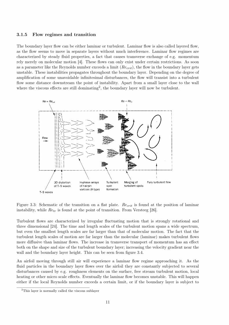
The boundary layer flow can be either laminar or turbulent. Laminar flow is also called layered flow,as the flow seems to move in separate layers without much interference. Laminar flow regimes arecharacterized by steady fluid properties, a fact that causes transverse exchange of e.g. momentumrely merely on molecular motion [4]. These flows can only exist under certain restrictions. As soonas a parameter like the Reynolds number exceeds a limit (Recrit), the flow in the boundary layer getsunstable. These instabilities propagates throughout the boundary layer. Depending on the degree ofamplification of some unavoidable infinitesimal disturbances, the flow will transist into a turbulentflow some distance downstream the point of instability. Apart from a small layer close to the wallwhere the viscous effects are still dominating2, the boundary layer will now be turbulent.
Figure 3.3: Schematic of the transition on a flat plate. Recrit is found at the position of laminarinstability, while Retr is found at the point of transition. From Versteeg [26].
Turbulent flows are characterized by irregular fluctuating motion that is strongly rotational andthree dimensional [24]. The time and length scales of the turbulent motion spans a wide spectrum,but even the smallest length scales are far larger than that of molecular motion. The fact that theturbulent length scales of motion are far larger than the molecular (laminar) makes turbulent flowsmore diffusive than laminar flows. The increase in transverse transport of momentum has an effectboth on the shape and size of the turbulent boundary layer; increasing the velocity gradient near thewall and the boundary layer height. This can be seen from figure 3.4.
An airfoil moving through still air will experience a laminar flow regime approaching it. As thefluid particles in the boundary layer flows over the airfoil they are constantly subjected to severaldisturbances caused by e.g. roughness elements on the surface, free stream turbulent motion, localheating or other micro scale effects. Eventually the laminar flow becomes unstable. This will happeneither if the local Reynolds number exceeds a certain limit, or if the boundary layer is subject to
2This layer is normally called the viscous sublayer
11

Figure 3.4: Schematic og laminar and turbulent boundary layers. The differences in momentumtransport is illustrated for both the (a) laminar boundary layer and (b) the turbulent boundarylayer. From Bertin [4].
an adverse pressure gradient. The initial disturbances will grow, eventually turning the laminar flowinto a turbulent flow regime. The stronger the disturbances, the faster this process will go.
For a turbulent boundary layer, the high velocity gradient at the wall increases the shear stress,resulting in higher skin friction for surfaces exposed to turbulent flow. Laminar flow is thereforefavorable over certain parts of an airfoil, due to the reduced viscous drag. However, the low velocitygradient and momentum transport close to the wall makes the flow more sensitive to separation, anundesirable effect for most airfoil flows.
3.1.6 Laminar separation bubbles
As the laminar boundary layer has less momentum transport close to the surface, it has less availablekinetic energy to overcome adverse pressure gradients. If the transition to turbulent flow does nothappen before the pressure gradient becomes adverse, separation can occur near the leading edgeeven for low angles of attack.
The separation will increase the amount of disturbances in the flow, leading to a rapid transition.After this transition occurs, the increased mixing will transport momentum towards the surface at ahigher rate than before, thus forcing the flow towards reattachment. If the airfoil Reynolds number ismore that approximately 7.0 · 104, the boundary layer can reattach, as long as the airfoil curvature oradverse pressure gradient is sufficiently small. In this case a laminar separation bubble is formed [15].However, a high curvature or adverse pressure gradient might cause the flow to remain separated fardownstream, causing the airfoil to stall. At the Reynolds numbers expected in the wind tunnel, thiseffect is expected.
This kind of stall can be very dramatic. If a laminar separation bubble close to the leading edgeburst, the airfoil will experience a very abrupt changes in lift and drag.
Modelling transisting flows is a complicated exercise with a high demand of computational powerand advanced models. As this is a mere masters project, this effects will not be modeled in detail,
12

Figure 3.5: Schematic of a laminar separation bubble. From Hu and Yang [11].
but only commented upon.
3.1.7 Lift and drag
With the pressure distribution known, the pressure forces acting on the effective body can be de-termined. Combined with viscous friction, the net forces acting in the streamwise and transversedirection can be calculated by integrating the pressure forces and the skin friction over the surface.The resultant forces are normally called drag in the streamwise direction, and lift in the transversedirection. The forces are often non–dimensionalised by dividing them by the dynamic pressure timesthe area in consideration. In a two dimensional case, the sectional lift and drag coefficients are givenas:
Cl =l
12ρU
2∞C
(3.8)
Cd =d
12ρU
2∞C
(3.9)
l and d being the lift and drag per unit span of the airfoil respectively. These are the forces creatingthe torque and thrust forces acting on a wind turbine.
It can be shown that a lifting force introduces circulation to the flow field. The relation between theinduced circulation and the lifting force is described by the Kutta–Jukowski theorem:
l = ρ∞U∞Γ (3.10)
Γ is the total circulation induced per unit span.
13

3.1.8 Tip loss
For an airfoil of infinite span, the flow will be completely two–dimensional (if one ignore the turbulentscales of motion). This makes the lift per unit span (and thus the circulation) independent on thespanwise position. For a wing of finite length, like a wind turbine blade, this is no longer the case.The high–pressure air on the pressure side of the blade will spill out around the tip towards thelow–pressure air on the suction side. This will decrease the pressure difference between the suctionand pressure side, reducing the lift towards the tip.
This tip effect will also induced spanwise velocity components over the blade, creating a vortexsheet behind the wing, that tend to roll up in large wing–tip vortices with high velocities and lowpressures. The trailing vortices induce an additional component of drag, as the effective angle ofattack is reduced due to downwash. This is known as vortex drag or induced drag and is known tobe proportional to the square of the lift coefficient divided by the aspect ratio, given an unswept,untapered wing [4].
It has been shown that the amount of circulation induced by the blade tends to zero as one approachesthe tip. The Prandtl tip loss factor describes this lift reduction, and is used in the BEM method toaccount for the tip effects.
As the wind turbine blade examined in this report has a sharp edge near the root as well, it is possiblethat a hub vortex will be present here. This will lead to the same effects as described above. But asthe relative velocity is far lower at this point, the effect of this vortex can be assumed to be lowerthan near the tip.
3.1.9 Rotational augmentation
Rotational augmentation or stall delay is still incompletely understood and characterized. But thereare strong indications that rotational effects can enhance blade section lift and delay stall on windturbine blades and propellers compared to a non–rotating reference. Several studies have beenperformed in order to examine the effects of rotation on a wind turbine, but the mechanisms behindthe effect of stall delay have not yet been determined.
A study of Schreck and Robinson did show that stall delay is associated with spanwise pressuregradients and chordwise ’pressure signatures’. One interpretation is that it is connected to centripetaland Coriolis forces [19].
The presence of centripetal and Coriolis forces will influence the flow field around the blade to acertain extent. Because of the blade rotation, the fluid particles in a blade–fixed reference systemwill experience an acceleration away from the blade. This acceleration imposes a small positiveradial velocity component on the fluid in the boundary layer. Due to the Coriolis effect, this radialvelocity component will induce a chordwise force that will act on the fluid in the boundary layer. Aforce acting in the chordwise direction can be interpreted as a favorable pressure gradient, delayingseparation [19].
It is however unclear what are the main driving factors behind this effect. The only thing clear isthat three dimensional effects are present, altering the flow field from the idealised case examined inthe BEM method.
14
3.2 The BEM–method
As seen in the previous chapter, the flow around the blades of a wind turbine is far more complicatedthan the two–dimensional flow assumed to be the case when making a BEM calculation. The twomain reasons for this are the three–dimensional effects caused by the rotation and the fact that theblades are of finite length.
As the blade sections are regarded non–interacting, these effects are neglected when using the BEMmethod. This simplifies the calculations dramatically, but introduces several errors. To accountfor this, some of the effects are addressed through modelling. The BEM method normally employstwo such models: Prandtls tip loss factor and Glauerts correction for high values of axial induction.These will be discussed in the following chapters.
The objective of a BEM–calculation is to determine the thrust and moment force caused by thefluid on each of the blade elements. The flow is normally divided into non–interacting annularstreamtubes of width dr. The aerodymaical forces acting on the corresponding blade element isfound, thus determining the axial and angular momentum changes of the air in the annular strip. Inorder to determine the lift and drag forces acting on each element, knowledge of the local angle ofattack (α) and flow velocity relative to the blade (Urel) needs to be obtained, as well as the bladetwist angle and chord length. As the design of the blades in this study is known, only the two firstquantities needs to be determined.
3.2.1 Axial induction factor
When the wind turbine extracts energy form the wind, the kinetic energy of the wind has to bereduced as it flows through the rotor plane of the turbine. The axial induction factor a describes theaxial speed reduction caused by the presence of the blades. This way, the axial speed at the rotorplane Ut is given by the relation Ut = U∞(1 − a). This is deducted from the definition of the axialinduction factor a:
a =U∞ − UtU∞
(3.11)
The axial induction factor is thereby a measure of the kinetic energy extraction from the wind. Asmall a indicates that little kinetic energy is extracted from the airflow, thereby indicating a lowefficiency. However, a high a implies that Ut is small, thus indicating a too high kinetic energyextraction. As this reduces the velocity at the rotor plane, the efficiency will be reduced as well.The optimum value of a can be found by using momentum theory on the flow around the turbine,yielding the following equation for the power coefficient, CP :
CP = 4a (1− a)2 (3.12)
The optimum found by differentiation, is known as the Betz limit, giving CPmax = 0.593 for a = 1/3.
15

Figure 3.6: The relations between α, ϕ, θ, the velocities and forces acting on a wind turbine bladeelement.
3.2.2 Angular induction factor
The circulation created by the lift force around the rotating blade, and the trailing vortices caused bythe finite length of the blade, induces rotation in the flow downstream of the wind turbine. Upstreamof the turbine, no rotation will be present. In a case where energy is extracted from the wind, thewake will be rotating in the opposite direction of the wind turbine rotor. The wake rotation can beregarded a net loss of energy. Because it is directly related to the torque generated by the fluid flow,a high tip speed ratio and low torque will lead to low losses due to wake rotation.
The angular component of the wind speed at the rotor plane is normally given as a fraction of thelocal rotational speed of the blade (ωra′), where a′ is the angular induction factor. Thus, the angularvelocity component of the relative wind speed at the rotor plane, will be given by the rotationalspeed of the blade, and the induced rotational speed. This way the tangential velocity componentat the rotor plane will be given as Wt = ωr(1 + a′).
a′ =Wt
ωr(3.13)
The relative inflow velocity (Urel) and the inflow angle (ϕ) can be calculated as long as the axialand angular induction factors are known. Using the definitions of the axial and angular inductionfactors, the effective inflow velocity and the inflow angle will be given by:
Urel =√
[U∞(1− a)]2 + [ωr(1 + a′)]2 (3.14)
tanϕ =U∞(1− a)ωr(1 + a′)
(3.15)
16

The angle of attack, α, is found by subtracting the twist angle, θ, from the inflow angle, ϕ. As α andUrel are known, sectional lift and drag forces acting on each element can be found. These forces aretransformed into normal and tangential forces through trigonometrical relations. The normal forcecoefficient (Cn) is defined as acting in the flow direction, thus acting as a thrust force. The tangentialforce coefficient (Ct) is defined as acting in the tangential direction, thus acting as a moment on thewind turbine axis. They are determined using the following equations:
Cn = Cl cosϕ+ Cd sinϕ (3.16)
Ct = Cl sinϕ− Cd cosϕ (3.17)
When the normal (thrust) forces and tangential (moment) forces for each blade element are found,the total thrust or torque can be found by integration along the blade.
3.2.3 Prantls tip loss
As a leakage of circulation is present at the tip, this needs to be corrected for in the BEM code. Itis clear that the forces acting on a blade element close to the tip should be lower than for a similarelement at the middle of the blade.
Prandtl showed that the circulation created by a rotating blade of a finite length tends exponentiallyto zero close to the tip. This is the basis of the Prandtl correction factor that can be added to theBEM equations; here given by the approximate formula introduced by Glauert [20]:
F =2π
cos−1
[e−B(R−r)
2r sin ϕ
](3.18)
This factor stays close to one for most radii, but goes quickly to zero close to the tip. This makesthe correction apply only for the elements close to the tip of the blade.
In the further equations, the solidity of the blades is defined as
σ(r) =C(r)B
2πr(3.19)
where B is the number of blades and r is the local radius. The corrected equations for the performancecalculations are given as [10]:
a =1
F4 sin2 ϕσCn
+ 1(3.20)
a′ =1
F4 sinϕ cosϕσCt
− 1(3.21)
dFx = 4πrρU2∞a(1− a)F (3.22)
17

dFz = 4πr2ρU∞ω(1− a)a′F (3.23)
Here dFx is the force acting per unit span of the blade in the streamwise (x) direction, while dFzis the force acting per unit span of the blade in the tangential (z) direction. If dFx is integratedalong the blade, the total thrust force (T ) is found. When dFz is multiplied with the local radiusand integrated along the blade to the tip, the total moment (M) is found.
T =∫ R
0dFxdr (3.24)
M =∫ R
0dFzrdr (3.25)
Close to the tip the Prandtl tip loss factor will go to zero. This will increase the axial inductionfactor toward one. This will reduce the angle of attack towards zero, reducing the forces acting onthe tip of the blade. However, if the angular induction factor is decreased towards minus one at arate faster than the axial induction factor, this will cause the angle of attack to increase toward thetip.
3.2.4 Glauerts correction for high values of a
As can be seen from equation 3.22, the thrust force will tend to zero as a tends to one. This is clearlyunphysical, as it is expected that the thrust will increase. The thrust coefficient will actually increasebeyond one. Glauert suggested a correction equation that should be used in the iterating process assoon as a increased beyond the value ac = 0.2.
a =12
[2 +K(1− 2ac)−
√(K(1− 2ac) + 2)2 + 4(Ka2
c − 1)]
(3.26)
K =F4 sin2 ϕ
σCn(3.27)
This correction factor has proven to give good results for wind turbine, and is normally used in bladeelement momentum calculations [10].
3.2.5 Hub loss
The fact that the blades has to be connected to a hub introduces three dimensional effects at theroot of the blade. The presence of a hub will affect the flow, inducing a speed up close to the root ofthe blade. This could make a simple omission of the hub area erroneous. In addition the presence ofa hub vortex will influence the lift and drag coefficients close to the root of the blade. This could beaddressed by introducing a hub loss factor. However, because the wind speeds are small compared tothe tip speeds for most operational conditions, the errors introduced here are assumed to be small.
18

3.2.6 Performance calculation
A flow chart for the calculation of a wind turbine performance with the Prandtl tip loss and Glauertscorrection factor is shown in figure 3.7. The calculation procedure is further described in Sætas projectthesis. The program PERFORMANCE and FORCE has been used in the following calculations.
19
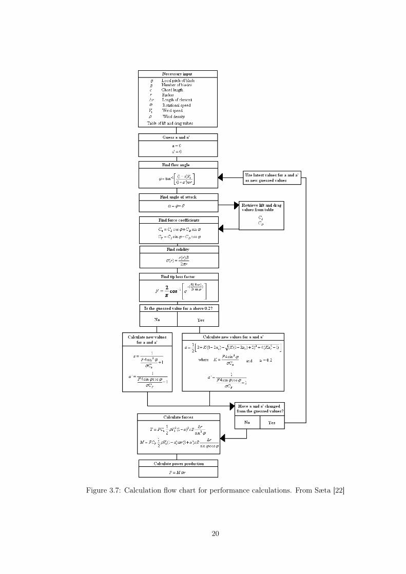
Figure 3.7: Calculation flow chart for performance calculations. From Sæta [22]
20

3.3 Numerical methods
The mathematical description of fluid motion is given by three laws of conservation: Conservationof mass, momentum and energy. Under assumptions that the flow is incompressible, and that thereexist a linear relation between shear and the velocity gradient, the fluid motion can be described bythe continuity equation and the well known Navier–Stokes equations.
The solution of these equations however, is not straightforward. Only a few, relatively trivial problemshave known analytical solutions. As soon as certain parameters (e.g the Reynolds number) exceedscertain limits, the flow regime becomes turbulent. The spatial scales of the turbulent motion in theflow are significantly larger than that of molecular motions, so that the fluid can still be regardeda continuum. But these scales are yet so small that a complete calculation of these motions isimpossible for most engineering problems.
3.3.1 The RANS equations
The most common way of addressing the issue with time–dependent, irregular motion is normallyto split all time-varying components of the flow into a mean and a fluctuating value, e.g Ui andui for the velocity in the xi direction. In this way a mean flow regime can be solved, with thefluctuating values being superimposed on the stationary solution. When this is introduced intothe governing equations, they can be averaged, resulting in the well known RANS equation and anaveraged continuity equation:
Uj∂Ui∂xj
= −1ρ
∂p
∂xi+
∂
∂xj
(ν
(∂Ui∂xj
+∂Uj∂xi
)− uiuj
)(3.28)
∂Uj∂xj
= 0 (3.29)
The turbulent motions are now reduced to one term in equation 3.28, called the Reynolds stresstensor −uiuj . The lack of an analytical solution to this term forces one to model these stresses, mostoften done by introducing the concept of a turbulent viscosity νt. This approach was suggested byBoussinesq in 1877, giving the following definition of the turbulent viscosity [5]:
−uiuj = νt
(∂Ui∂xj
+∂Uj∂xi
)− 2
3kδij (3.30)
where k = 12uiui is known as the mean turbulent kinematic energy, and δij as the Kronecker delta.
By introducing this concept, it can be seen that the magnitude of the different Reynolds stressesmust be equal, resulting in an assumption of isotropic turbulence. Isotropic turbulence is known tobe an exception rather than the rule, yet models using this concept still yield quite good results inmany cases. Several attempts have been made to model the different stresses separately, using so–called Reynolds Stress Models (RSM). However, these tend to be quite computationally demanding.Moreover, the increased complexity of these models have not yet proven to yield correspondingly moreaccurate results [26]. The turbulent viscosity is normally modelled by introducing the dissipation rateof k, ε. This approach was standardized by Jones and Launder when they introduced the k–ε–modelin 1972. Another approach was introduced by Kolmogorov, and refined by Wilcox. They chose to
21

model the turbulent viscosity by introducing the concept of the spesific dissipation rate, ω that hasdimensions of (time)−1.
νt =µtρ
= Cµk2
ε=k
ω(3.31)
The two different approaches shown above are the basis of two of the most used two–equationturbulence models, namely the k–ε– and k–ω–model. In order to calculate νt, transport equationshave to be made for the two unknown variables. The basis of two–equation turbulence modelling liesin the modelling or derivation of the transport equations for these two unknowns.
Several models for the transport equation for k are available, being the basis of most one–equationturbulence models. The challenge in two–equation turbulence modelling lies in the transport equationfor the second unknown.
3.3.2 Turbulence models
The k–ε–model
The first k–ε–model was proposed in 1972 by Jones and Launder, when they modelled a transportequation for ε [14]. The effort has been criticised for being too much of a ’drastic surgery’ to theoriginal equations [28], however it is still one of the most used turbulence models available.
Dρk
Dt=
∂
∂xj
[(µ+
µtσk
)∂k
∂xj
]+Gk − ρε (3.32)
Dρε
Dt=
∂
∂xj
[(µ+
µtσε
)∂ε
∂xj
]+ C1ε
ε
kGk − C2ερ
ε2
k(3.33)
Gk = −ρuiuj∂Uj∂xi
(3.34)
Gk is the production of k, and is through the Boussinesq approximation given as Gk = 2µt(SijSij).The strain–rate tensor is given as: Sij = 1/2
(∂Ui∂xj
+ ∂Uj
∂xi
). The coefficients in the model are presented
in table 3.1. The model is derived under the assumption that the flow is fully turbulent, and thatthe effect of molecular viscosity is neglectible. The model is therefore only valid for fully turbulentflows, and cannot predict transition.
Even if the model is widely used, it has major deficiencies, especially in recirculation areas and areasof rapid strain. The simplification introduced through the Boussinesq–approximation makes theturbulent stresses proportional to the strain–rate. µt is not a scalar in reality, therefore in cases ofhigh anisotropy better results can be obtained by modelling the Reynolds stresses separately, using aReynolds Stress Model (RSM). As this is quite computationally demanding, and the solutions tendto be more unstable than general two–equation solutions this approach is not used in this study.
22
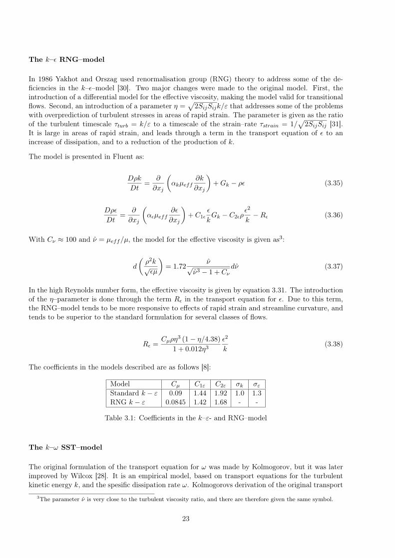
The k–ε RNG–model
In 1986 Yakhot and Orszag used renormalisation group (RNG) theory to address some of the de-ficiencies in the k–ε–model [30]. Two major changes were made to the original model. First, theintroduction of a differential model for the effective viscosity, making the model valid for transitionalflows. Second, an introduction of a parameter η =
√2SijSijk/ε that addresses some of the problems
with overprediction of turbulent stresses in areas of rapid strain. The parameter is given as the ratioof the turbulent timescale τturb = k/ε to a timescale of the strain–rate τstrain = 1/
√2SijSij [31].
It is large in areas of rapid strain, and leads through a term in the transport equation of ε to anincrease of dissipation, and to a reduction of the production of k.
The model is presented in Fluent as:
Dρk
Dt=
∂
∂xj
(αkµeff
∂k
∂xj
)+Gk − ρε (3.35)
Dρε
Dt=
∂
∂xj
(αεµeff
∂ε
∂xj
)+ C1ε
ε
kGk − C2ερ
ε2
k−Rε (3.36)
With Cν ≈ 100 and ν̂ = µeff/µ, the model for the effective viscosity is given as3:
d
(ρ2k√εµ
)= 1.72
ν̂√ν̂3 − 1 + Cν
dν̂ (3.37)
In the high Reynolds number form, the effective viscosity is given by equation 3.31. The introductionof the η–parameter is done through the term Rε in the transport equation for ε. Due to this term,the RNG–model tends to be more responsive to effects of rapid strain and streamline curvature, andtends to be superior to the standard formulation for several classes of flows.
Rε =Cµρη
3 (1− η/4.38)1 + 0.012η3
ε2
k(3.38)
The coefficients in the models described are as follows [8]:
Model Cµ C1ε C2ε σk σεStandard k − ε 0.09 1.44 1.92 1.0 1.3RNG k − ε 0.0845 1.42 1.68 - -
Table 3.1: Coefficients in the k–ε- and RNG–model
The k–ω SST–model
The original formulation of the transport equation for ω was made by Kolmogorov, but it was laterimproved by Wilcox [28]. It is an empirical model, based on transport equations for the turbulentkinetic energy k, and the spesific dissipation rate ω. Kolmogorovs derivation of the original transport
3The parameter ν̂ is very close to the turbulent viscosity ratio, and there are therefore given the same symbol.
23

equations was probably (according to Wilcox) made by dimensional analysis and physical reasoning.A quite different path than Jones and Launder chose.
The k–ω–model is known to be the model of choice in the viscous sublayer, and it allows simpleDirichlet boundary conditions to be specified walls [16]. This makes it possible to apply the modelthroughout the boundary layer. However, in the wake region of the boundary layer, the model isquite sensitive to freestream values of ω. The fact that this deficiency is not shared by the k–ε–model,gave rise to Menters idea of coupling them.
Through the introduction of blending functions (F1 and F2), Menter combined the two models inhis Shear Stress Transport model; the k–ω–model was applied in the near wall region, while thek–ε–model was applied in the outer wake region and the free shear layers [16]. He also made somemodification of the definition of the eddy viscosity in order to account for the transport of theprincipal turbulent stress.
The model used in Fluent is given as [8]:
Dρk
Dt=
∂
∂xj
[(µ+
µtσk
)∂k
∂xj
]+ G̃k − Yk (3.39)
Dρω
Dt=
∂
∂xj
[(µ+
µtσω
)∂ω
∂xj
]+Gω − Yω +Dω (3.40)
µt =ρk
ω
1
max(
1α∗ ,
SF2α1ω
) (3.41)
σk =1
F1/σk,1 + (1− F1) /σk,2(3.42)
σω =1
F1/σω,1 + (1− F1) /σω,2(3.43)
G̃k = min(−ρu′iu′j
∂uj∂xi
, 10ρβ∗kω)
(3.44)
Gω = − ανtρu′iu
′j
∂uj∂xi
(3.45)
Because the model is using a k–ε formulation in the outer region, a cross diffusion term appears asthe k–ε–model is transformed into a k–ω formulation. This term is given as:
Dω = 2 (1− F1) ρσω,21ω
∂k
∂xj
∂ω
∂xj(3.46)
The diffusion terms (Yk and Yω), as well as the model constants are excluded here. A completedescription of the turbulence model is found in the Fluent user guide, or in the Menter article [16][8].
24

The Spalart–Allmaras model
The Spalart–Allmaras turbulence model is a one–equation model that has been designed specificallyfor aerospace applications, and it is therefore a model of choice regarding wall–bounded flows. It hasalso proven to yield good results for boundary layers with adverse pressure gradients.
As a one equation model it has certain shortcomings regarding abrupt changes from wall–boundedto free shear flow and prediction of the decay of homogeneous isotropic turbulence. However, themodel has given promising results for turbomachinery applications [8].
The model uses a modified turbulence viscosity as the transported variable, the transport equationgiven as:
Dρν̃
Dt= Gν +
1σν̃
[∂
∂xj
((µ+ ρν̃
∂ν̃
∂xj
)+ Cb2ρ
(∂ν̃
∂xj
)2]− Yν (3.47)
µt = ρν̃
((ν̃/ν)3
(ν̃/ν)3 + C3v1
)(3.48)
In the model, Gν is the production of ν̃ and Yν is the destruction. Model constants and equationsfor the production and destruction of ν̃ can be found in the Fluent user guide [8]. The modifiedturbulence viscosity is set to zero at walls.
3.3.3 Boundary conditions
Inlet and outlet boundary conditions
In order to close the equations in a CFD problem, boundary conditions have to be determined. Atthe inlet, flow velocity and turbulent properties are normally set. The flow velocity in this problemis known from the measurements. Apart from that, two turbulence properties needs to be set inorder to close the two turbulent transport equations. Here this is done by specifying a turbulenceintensity (TI) and a turbulent viscosity ratio (ν̂). The turbulent intensity is defined as the root meansquare value of the velocity fluctuations, divided by the mean flow velocity [8]. With the Boussinesqassumption of isotropic turbulence, one gets:
k =23
(U∞TI)2 (3.49)
The turbulent viscosity ratio is defined as the ratio between the turbulent and the molecular viscosity.It is normally given as ν̂ = µt/µ, or in terms of the kinematic viscosity, as the flow is incompressible.The relationship between the spesific dissipation rate and the turbulent viscosity ratio is given as:
ω = ρk
µ
(µtµ
)−1
(3.50)
Knowing the spesific dissipation rate, the dissipation rate (ε) can be found using equation 3.31.
25

At the outlet a static pressure was set. Compared to a determination of the outflow velocity orvelocity angle, this method is known to give better convergence in case backflow occurs. In casebackflow occurs, turbulent properties needs to be determined for this ’inflow’. This was done bydetermining a high turbulence intensity while keeping the viscosity ratio determined at the inlet.
Periodic boundary condition
When the wind turbine is modelled, the flow is assumed to be rotationally periodic. This is a validassumption as long as the wind tunnel is modelled as a circular tube, and the influence from non–rotational geometries (like the wind turbine tower or hub irregularities) are excluded. This has beendone in the three dimensional simulations in order to reduce the size of the numerical model to onethird of the physical model.
The periodic boundaries are placed 120◦ apart, with one wind turbine blade placed in between.The boundaries are specified so that there is no pressure drop across them. When calculating flowvariables at one cell at the periodic boundary, its neighbor cell on the other side of the boundary willbe the cell adjacent to the opposite periodic boundary [8]. Explained in another manner, the flowinto one periodic boundary will flow out of the opposite one.
Wall boundary condition
Wall boundaries are determined so that there are no velocity components normal to the wall. Thevelocity gradient close to the wall can be specified directly, or the no–slip condition can be applied.
All viscous flows are significantly affected by the presence of walls. For physical, non–moving walls,the no–slip condition has to be fulfilled. This gives rise to a shear, affecting both the velocity andthe turbulent properties of the flow. While the k–ω–model can be applied throughout the boundarylayer, the k–ε models are only valid for fully turbulent flow. This is problematic in the viscoussublayer, wheree the viscous stresses are dominant.
There are two main ways of achieving boundary conditions for wall–bounded flows.
• The wall–function approach uses the law of the wall, and semi–empirical relations to determinethe velocity and turbulent properties in the logarithmic region. This reduces the refinementclose to the surface, resulting in faster computations.
• The near–wall model approach uses grids that resolves the viscous sublayer, and uses formulasfor near–wall turbulent quantities. The need for a fine mesh increases the computing time, butthe approach is known to give better results, especially for low–Reynolds–number flows.
For most high Reynolds–number flows with finite wall shear, the law of the wall is valid for a thinregion close to the surface. The viscous sublayer and the logarithmic layer both has well–definedvelocity distributions under these conditions, that are used to determine the mean velocity close tothe wall. In the viscous sublayer, ranging from 0 ≤ y+ < 5 the velocity distribution is known to begiven by u+ = y+. In the fully turbulent logarithmic layer 70 ≤ y+ < 300, the velocity is known tobe described by the logarithmic law u+ = 1
κ ln (y+) + C+ [18].
The wall function approach is used by the k–ε–models, assuming that the dissipation rate andproduction of turbulent kinetic energy is in equilibrium in the logarithmic layer. This gives the
26
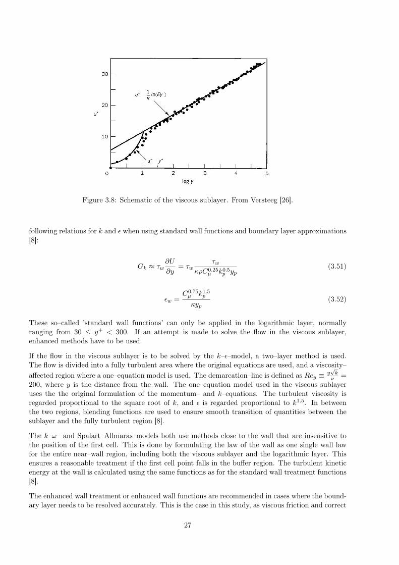
Figure 3.8: Schematic of the viscous sublayer. From Versteeg [26].
following relations for k and ε when using standard wall functions and boundary layer approximations[8]:
Gk ≈ τw∂U
∂y= τw
τwκρC0.25
µ k0.5p yp
(3.51)
εw =C0.75µ k1.5
p
κyp(3.52)
These so–called ’standard wall functions’ can only be applied in the logarithmic layer, normallyranging from 30 ≤ y+ < 300. If an attempt is made to solve the flow in the viscous sublayer,enhanced methods have to be used.
If the flow in the viscous sublayer is to be solved by the k–ε–model, a two–layer method is used.The flow is divided into a fully turbulent area where the original equations are used, and a viscosity–affected region where a one–equation model is used. The demarcation–line is defined as Rey ≡ y
√k
ν =200, where y is the distance from the wall. The one–equation model used in the viscous sublayeruses the the original formulation of the momentum– and k–equations. The turbulent viscosity isregarded proportional to the square root of k, and ε is regarded proportional to k1.5. In betweenthe two regions, blending functions are used to ensure smooth transition of quantities between thesublayer and the fully turbulent region [8].
The k–ω– and Spalart–Allmaras–models both use methods close to the wall that are insensitive tothe position of the first cell. This is done by formulating the law of the wall as one single wall lawfor the entire near–wall region, including both the viscous sublayer and the logarithmic layer. Thisensures a reasonable treatment if the first cell point falls in the buffer region. The turbulent kineticenergy at the wall is calculated using the same functions as for the standard wall treatment functions[8].
The enhanced wall treatment or enhanced wall functions are recommended in cases where the bound-ary layer needs to be resolved accurately. This is the case in this study, as viscous friction and correct
27

prediction of separation is an important factor when determining the forces acting on an airfoil.
3.3.4 Discretisation
In a numerical solution, the fluid and flow properties are normally calculated for all cell centers. Butas we are using a Control Volume Method, the fluxes at the cell faces also need to be known. Thefact that the solution is not continuous, forces us to use a differencing scheme. The most intuitiveone is the ’central differencing scheme’ that applies simple linear interpolation between values in theclosest cell centers in order to find fluid properties at cell faces.
In a problem where convection is a dominant cause of transportation, this might not be appropriate.It is rather expected that the cell center value of a specific property will be more influenced by thecorresponding value in the upwind cell than in the downwind. This fact has lead to the ’upwinddifferencing scheme’ that takes the flow direction into account, and uses only upwind cell centervalues for interpolation at cell faces.
As the accuracy of the upwind differencing scheme is only first order in terms of truncation errors, itis vulnerable for numerical errors. However, first order schemes tend to be numerically stable, andsuitable for initial simulations. In order to reduce the truncation errors, higher order differencingschemes must be used. FLUENT has the option for a ’second order upwind differencing scheme’ anda QUICK scheme. Both these schemes have been used in the calculations.
The QUICK scheme uses quadratic interpolation, thus reducing the truncation errors. It is howevermore exposed to numerical divergence.
3.3.5 Numerical solution strategies
The equations governing a complicated fluid flow problem have no analytical solution. Numericalapproaches must therefore be applied. As the equations 3.28 and 3.29 are coupled, they cannot besolved separately. One of the most common solutions strategies is called SIMPLE.
The procedure uses a guessed pressure field as the starting point (p∗). On the basis of this, thediscretised momentum equations (3.28) are solved. The resultant velocity field does not necessarilysatisfy the continuity equation, therefore the pressure and velocity fields must be corrected by acertain value to account for this (pnew = p∗+ p′ ). In the end the rest of the transport equations aresolved.
As the old value of a scalar (e.g. p∗) is corrected by the term p′, the equation is susceptible todivergence. The correction term might be too large, and the changes are normally damped by anunder-relaxation factor. Due to this, the correction equation for the pressure is given as:
pnew = p∗ + αpp′ (3.53)
where αp is the under–relaxation factor. If this is kept at one, the solution is in danger of divergence.If it is kept close to zero, nothing will happen. The trick is to find the right value in order to speedup convergence without risking divergence.
The SIMPLE and SIMPLEC algorithm are both used in this project. The differences between themare marginal, and further information can be found in Versteeg [26].
28

Chapter 4
Experimental results
4.1 Experimental setup
The turbine examined in this project has been developed for testing in the NTNU wind tunnel. Thewind tunnel has a cross section of 2.7 m x 1.9 m, and a test section approximately 11 m long.
The wind turbine blades are connected to a rotating nacelle. The blades can be pitched about theblade quarter chord, but this pitch angle (∆θ) was set to zero in the experiment. This nacelle isconnected by an axis to a transmission belt that is attached at the rear of the hub. This transmissionbelt transfers the moment to a generator mounted beneath the wind tunnel floor. The generatoris connected to a full–frequency converter, making it possible to control the rotational speed of therotor. A torque gauge is mounted in the hub in order to measure the moment on the transmissionaxis. This data was logged by a computer.
The nacelle and blades are mounted on a cylindrical hub. This hub has a diameter of 0.09 metresand is 0.56 m long. Thorough measurements of the geometry was performed, and the hub was latermodelled in GAMBIT.
The hub is mounted on a tower that consists of several cylindrical elements with different diametersmounted on top of each other. The frontal area of the tower is approximately 0.053 m2. The towerheight was measured to be 0.82 m high, keeping the tip of the blade 0.37 m from the nearest windtunnel wall. This distance is thought to be enough to prevent the blades from entering the windtunnel boundary layer.
The wind turbine was mounted on a weight that can measure forces in three dimensions. Howeveronly the thrust force was measured. The thrust gauge readings was logged by a computer.
The free stream velocity was measured using a pitot tube. The measurements was taken upstreamof the wind turbine, some distance to the side, in order to escape the influence of the wind turbine.
All measurements was logged at a frequency of 500 Hz, with a logging time of 15 s. This resulted ina total number of samples of 7500. Both mean values and standard deviations (σ) were collected.
The temperature was measured using a regular digital thermometer and the total (atmospheric)pressure using a weatherglass.
29

Figure 4.1: A schematic of the experimental setup in the wind tunnel
4.2 Calibration
The pitot tube calibration curve was already known, but the torque and thrust gauges had to becalibrated. This was done using weight elements with a known mass. The sensors are known torespond linearly to increased torque and thrust forces. Linear regression was used to obtain thecorrect relation between the sensor signals and the real forces acting on the turbine. The calibrationcurves and data can be found in appendix A.1.
10 and 14 measurements were conducted for the torque and thrust sensor respectively. The calibrationresults yielded a correlation of 0.9999 and 0.9995 respectively, thereby the systematic error can beexpected to be rather small.
4.3 Results
Measurements of the total pressure and temperature were done. This made it possible to estimatethe density of the air using the ideal gas law. Combined with the dynamical pressure measured bythe pitot tube, the wind speed in the wind tunnel was found:
U∞ =√
2q∞ρ
(4.1)
Knowing the rotational velocity, the tip speed ratio was determined.
The torque and thrust forces were measured directly, and the coefficients of performance was calcu-lated using the known free stream velocity, density and the rotor area. The calculations was doneusing equation 3.1 and 3.2.
A free stream Reynolds number based on the rotor diameter was obtained. The mean kinematic
30

viscosity measured in the wind tunnel was determined using Sutherlands equation that can be usedfor air for temperatures below 3000 K [4]:
µ = 1.458 · 10−6 T 1.5
T + 110.4(4.2)
Mean σ Max MinVelocity 9.97 m/s 0.165 m/s 10.56 m/s 9.87 m/sTotal pressure 99.97 kPa - - -Density 1.173 kg/m3 0.002 kg/m3 1.176 kg/m3 1.1704 kg/m3
Temperature 23.848◦C 0.404◦C 24.4◦C 23.0◦CReynolds number 6.38x10⁵ 0.12x10⁵ 6.77x10⁵ 6.31x10⁵
Table 4.1: Mean, maximum and minimum values, as well as the standard deviation of the results inthe wind tunnel experiment.
The Reynolds number can then be found from equation 4.3 and the ideal gas law, based on the velocityupstream of the wind turbine, the wind turbine diameter (d), the pressure and the temperature:
Re =Ud
µ
p
RT(4.3)
Measurements were done with varying rotational speed of the wind turbine, keeping all other pa-rameters constant. A small temperature rise was observed during the experiment. This changes thedensity and viscosity of the air somewhat, but was observed to have only a small effect on the windtunnel Reynolds number. The temperature rise is quite normal, as some of the work done by thewind turbine fan is transformed into heat, making the temperature in the wind tunnel rise.
The measured values of the torque and thrust forces was used to generate a CP and CT curve.
Figure 4.2: Measured CP and CT curves. The bars indicate the measured standard deviation.
The standard deviations are indicated in figure 4.2. It is clear that there are some considerabledynamic effects causing large fluctuations in both torque and thrust forces between λ = 4 and λ = 5.As the tip speed ratio was reduced below 5, we know that the local angle of attack is increasing overthe blade. As the efficiency of the wind turbine is reduced here, this could indicate that the dynamiceffects are related to separation.
31

It is important to notice that the method of changing the rotational speed of the wind turbine makesReynolds number effects more dominant, compared to a case where the rotational speed was keptconstant, with a varying free stream velocity. For most tip speed ratios above 2 (where the relativeinflow angle at the tip is less than 30◦), the Reynolds number at the tip will to a large extent bedetermined by the rotational speed. This makes the tip Reynolds number in this experiment varywith a factor of 10 (see figure 7.1).
A more thorough investigation of these results will be done using the BEM method and CFD simu-lations.
32
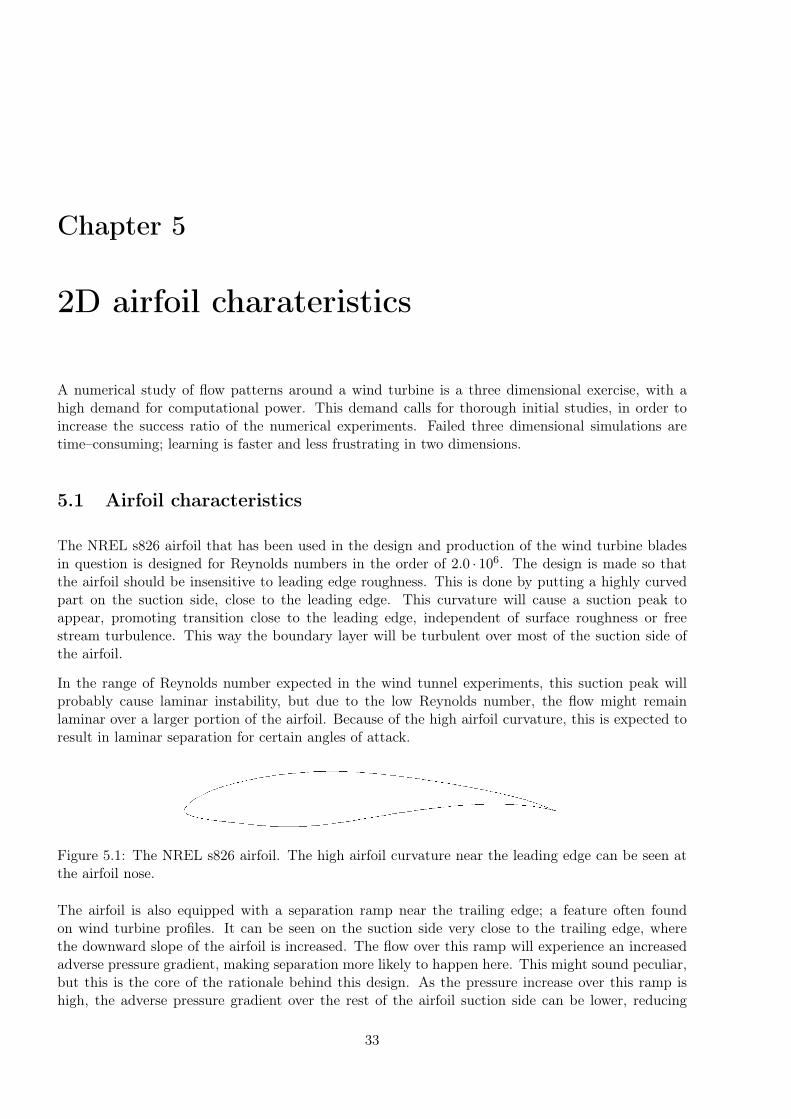
Chapter 5
2D airfoil charateristics
A numerical study of flow patterns around a wind turbine is a three dimensional exercise, with ahigh demand for computational power. This demand calls for thorough initial studies, in order toincrease the success ratio of the numerical experiments. Failed three dimensional simulations aretime–consuming; learning is faster and less frustrating in two dimensions.
5.1 Airfoil characteristics
The NREL s826 airfoil that has been used in the design and production of the wind turbine bladesin question is designed for Reynolds numbers in the order of 2.0 · 106. The design is made so thatthe airfoil should be insensitive to leading edge roughness. This is done by putting a highly curvedpart on the suction side, close to the leading edge. This curvature will cause a suction peak toappear, promoting transition close to the leading edge, independent of surface roughness or freestream turbulence. This way the boundary layer will be turbulent over most of the suction side ofthe airfoil.
In the range of Reynolds number expected in the wind tunnel experiments, this suction peak willprobably cause laminar instability, but due to the low Reynolds number, the flow might remainlaminar over a larger portion of the airfoil. Because of the high airfoil curvature, this is expected toresult in laminar separation for certain angles of attack.
Figure 5.1: The NREL s826 airfoil. The high airfoil curvature near the leading edge can be seen atthe airfoil nose.
The airfoil is also equipped with a separation ramp near the trailing edge; a feature often foundon wind turbine profiles. It can be seen on the suction side very close to the trailing edge, wherethe downward slope of the airfoil is increased. The flow over this ramp will experience an increasedadverse pressure gradient, making separation more likely to happen here. This might sound peculiar,but this is the core of the rationale behind this design. As the pressure increase over this ramp ishigh, the adverse pressure gradient over the rest of the airfoil suction side can be lower, reducing
33

the possibility of separation. If the flow separates, the separation will tend to be confined to theseparation ramp area, reducing the dynamic stall effects. This has proven to be an effective way ofreducing dynamic loads on stall regulated wind turbines.
This trap both makes separation occur quite early but also delays full stall. Because separationtends to alter the effective shape of the airfoil, this will tend to smooth lift and drag curves, causingstall to happen more smoothly. This is favorable, as a wind turbine exposed to turbulent inflow willexperience large variations in local angle of attack.
The airfoil is cambered, and will therefore generate lift at zero angle of attack.
In lack of experimental data, results from XFOIL has been used as an input for BEM calculationsand comparison with CFD results. XFOIL is known to give accurate results for airfoils within a largerange of Reynolds numbers. Studies have shown that XFOIL is able to predict airfoil forces quiteaccurately, even though the actual position of the transition point or the spatial extent of separationbubbles might not be correctly predicted at low Reynolds numbers [29] [25].
5.2 XFOIL study
5.2.1 Analysis of transition criteria
In order to examine the airfoil performance in an efficient manner, XFOIL was used to generatelift and drag curves for different Reynolds numbers and transition criteria. Choosing a reasonabletransition criteria is important because the actual position of the transition point has a large influenceon airfoil performance.
The flow around a smooth airfoil of infinite length moving in still air is known to transist fromlaminar to turbulent flow as soon as the level of disturbances exceeds a certain limit. The transitionpoint can be predicted with a reasonable accuracy by using the en–criteria, where n or Ncrit is theamplification factor of the most–amplified frequency which triggers transition [18]. The recommendedvalue for Ncrit is normally 9. This method is only appropriate in situations where the growth oftwo–dimensional Tollmien–Sclichting waves are the dominant cause of the transition.
However, this is not expected to be the case for the flows examined in this study. There are threemain effects that most probably will cause transistion to occur considerably closer to the leadingedge than what is the case in the idealised two dimensional case mentioned above.
1. The flow around the wind turbine is swirling, where substantial three–dimensional effects arepresent. These effects will most probably disturb the two–dimensional Tollmien–Schlichtingwaves, dictating a different path to transition.
2. The turbulence level in the wind tunnel is expected to be in the order of 0.7% [9], introducingexternal disturbances that will hasten the transition.
3. The wind turbine blades are not completely smooth, and have some small edges and scratchesnear the leading edge. In case this roughness turns out to be a cause of transition, the linearinstability theory will fail to predict the transition point [4].
Depending on the magnitude of these disturbances, transition might occur quite close to the leadingedge, forcing a turbulent flow regime over most of the airfoil.
34

The effects of rotation on transition are very hard to determine. There are indications that rotationmight hasten transition due to introduction of three dimensionality. However, this effect has beenexcluded in the following discussion. Only the two last effects will be discussed. In order to mimicthe effect of roughness or free–stream turbulence the amplification factor can be given a lower value.This will cause transition to occur closer to the the point of laminar instability, thus imitating theother physical effects.
By varying the transition criteria, l/d curves were calculated for three different Reynolds numbers.
Figure 5.2: L/D–ratios for s826 at α = 7◦ with varying Ncrit and varying Reynolds numbers.
Figure 5.2 shows how both conservative (high Ncrit) and progressive (low Ncrit) transition criteriagives reduced lift to drag ratios. When Ncrit is given a high value, laminar separation will occur onboth sides of the profile for most angles of attack. This will deform the effective shape of the airfoiland significantly reduce the airfoil performance.
When Ncrit is given a low value, the flow is turbulent over most of the airfoil. The lift is not muchaltered, so the increased viscous drag accounts for most of the l/d reduction.
It is clear from figure 5.2 that we face an airfoil efficiency reduction as the Reynolds number is reduced,regardless the transition criteria. A reduction of the Reynolds number do by definition imply thatviscous effects becomes more dominating, increasing viscous drag. In addition the thickness of theboundary layer will increase with decreasing Reynolds number, deforming the airfoil, leading toincreased form drag or less lift.
The Reynolds number effect will be important when calculating the wind turbine performance.
5.2.2 Lift and drag curves
On the basis of figure 5.2, three different transition criteria were used in the further studies; Ncrit =0.01 with more or less instant transition. Ncrit = 3.0 was chosen for a moderate case, somewherein between. Ultimately, Ncrit = 9 was chosen as the other ’extreme’. These was used to produceL/D–ratios for different angles of attack with a Reynolds number of 1.0 · 105.
The presence of laminar separation bubbles in the case where Ncrit is set to 9 is clear from figure5.3. For moderate angles of attack the deformation of the airfoil tend to both increase the drag and
35

Figure 5.3: L/D–ratios, lift and drag coefficients for different α, using three different transitioncriteria. Re = 1.0 · 105
reduce the lift. A typical laminar separation bubble can be seen in figure A.1 in the appendix.
As seen in figure 5.3, the airfoil has a somewhat better performance with conservative transitioncriteria (Ncrit = 9.0) in the early stall area (10◦ < α < 15◦). This is caused by the presence of alaminar separation bubble near the leading edge. In this bubble, the pressure gradient is very small,maintaining a lower pressure over a larger portion of the airfoil. This way the effective curvature ofthe airfoil leading edge is reduced, reducing the adverse pressure gradient. This moves the actualseparation point closer to the trailing edge, compared to a case where transition occurs before laminarseparation. Thus, the lift is increased. However, as the angle of attack exceeds 15◦, the laminar bubbleburst, resulting in full stall from the leading edge. As the stall will be very abrupt, this kind of stallcan result in severe dynamic effects. Detailed graphs and figures of this transition procedure is foundin appendix A.4.
The Ncrit = 3.0 regime is also affected by laminar separation, seen as an increase in lift for moderateangles of attack. However, no dramatic stall is observed here.
In the wind turbine case, it seems clear that a Ncrit of 9 is too conservative. The presence ofrotation, free–stream turbulence and roughness will most probably force transition to occur before the
36

Tollmien–Schlichting linear instability occurs for moderate angles of attack. It is therefore expectedthat a lower Ncrit will imitate the actual processes more actually.
Assuming the transition to occur near the leading edge for all angles of attack might be a to progres-sive choice. However, an analysis of all three cases might be interesting when comparing the BEMresults to the experimental data.
37

5.3 CFD study
5.3.1 Methods
A 2D model of the NREL s826 airfoil was made using GAMBIT. The numerical domain was extended12.5C upstream and 20C downstream of the airfoil. These are recommended values used in severalstudies in the literature, and the solutions sensitivity to the size of the numerical domain was thereforenot tested. A structured grid was used close to the airfoil, while both structured and unstructuredgrids was used in the rest of the numerical domain.
The CFD–study was performed in FLUENT, with a focus on examination of how different turbulencemodels and grid resolutions affected the solution. This was done in order to reduce the computationaleffort in the three dimensional case. The sensitivity to the following parameters was tested:
• Choice of turbulence model
• Freestream turbulence level sensitivity
• Grid resolution sensitivity
• Reynolds number sensitivity
Figure 5.4: The ’O I’ grid that has been used in the two dimensional studies of the NREL s826 airfoil.
A Reynolds number of 1.0 · 105 was used in the CFD–calculations if not stated otherwise. This wasachieved by adjusting the fluid viscosity and density, keeping the inflow velocity at 10 m/s in allsimulations.
A turbulence intensity between 1.0% and 0.5% is expected in the wind tunnel [9]. As a base case,the turbulence intensity close to the airfoil was put set to 1% in most of the calculations. It was latershown, as seen in figure 5.6, that the fully turbulent solutions showed little sensitivity to the freestream turbulence level. A turbulence viscosity ratio was also defined at the inlet. It was definedusing the approximation ε = 2k in order to ensure that the turbulence level was decreasing as theflow approaced the airfoil.
The outlet was set as a constant pressure boundary, and the airfoil surface as a smooth wall. Bothstandard wall functions and enhanced wall treatment were used.
38

The SIMPLE algorithm was used to couple the pressure and velocity field, and 2. order upwinddifferencing schemes was applied on the flow variables. Only stationary solutions was obtained.
5.3.2 Grid resolution sensitivity
In order to solve the flow field around an airfoil, the grid needs to be fine enough to capture the flowgradients. As the flow gradients are generally larger close to solid surfaces, the cell size can generallybe enlarged with distance from these surfaces.
A structured boundary layer grid was constructed close to the airfoil. This was done in order toensure a good resolution of the boundary layer flow. A structured grid makes it easy to control ofthe transverse grid resolution close to the airfoil surface. It it possible to combine this with both astructured or an unstructured grid in the rest of the numerical domain. In the 3D-case, unstructuredgriding is preferable due to its simplicity. The downside of unstructured grids is the fact that thenumber of cells tends to increase. In addition unstructured grids tend to be more numerically unstablethan structured grids. This calls for an thorough investigation of different griding possibilities, andfurther how this affects the solution.
An initial grid independence study was performed in order to be sure that the solutions obtained inthe later sensitivity analyses were consistent. The grids used in the study are presented in table 5.1.The fully turbulent k–ω SST model was used in the calculations.
Using the six different grid presented in table 5.1, lift drag polars were created using the SST–model. The results are presented in figure 5.5. It is clear that there is an outstanding consistencybetween the CFD simulations and the XFOIL results. The solution seems to be independent of thegrid resolution, apart from grid ’O IV’. Examining table 5.1, there is a strong indication that thechordwise grid resolution has not been good enough.
Chordwise grid resolution
As there are chordwise flow gradients over the airfoil surface, it is important that there are enoughcells on the airfoil surface. First of all, the airfoil geometry needs to be captured. Second, thechordwise flow gradients needs to be captured. Because of this, several grid–points are needed inareas of high curvature and in areas with high rates of change in the chordwise direction. Thisapplies to the leading and trailing edge, as well as close to separation– and reattachment–points. As
Grid C I C II O I O II O III O IV# cells 41 000 100 000 27 188 19 570 18 920 17 473# nodes on airfoil 210 300 366 248 248 141# nodes normal to airfoil 100 200 - - - -yp 10−4C 10−4C 10−4C 10−4C 2 · 10−4C 2 · 10−4C
Nodes in BL - - 45 35 30 30BL growth rate - - 1.12 1.12 1.15 1.15BL height - - 0.136C 0.043C 0.087C 0.087C
Table 5.1: Grid parameters for grids used in the fist part of the grid sensitivity study. There aretwo structured C-shaped grids (C I and C II), and four unstructured grids with a structured O-gridwrapped around the airfoil (O I - O IV).
39

Figure 5.5: Initial grid independence study. The XFOIL results has been obtained using a Ncrit of0.01 to indicate turbulent flow.
separations and reattachment–points move with the flow conditions, the grid was only refined towardthe leading and trailing edge.
Figure 5.6: Lift and drag coefficients for grids with different number of grid points on the airfoilsurface. The filled and open figures are indicating calculations with a TI at the airfoil of 1 % and 0.2% respectivly.
Examining the results obtained from the initial study, one sees that the number of grid–points on theairfoil were varying from 366 to 141. The results are presented in figure 5.6. It is clear that grid ’OIV’ is unable to predict the correct drag coefficient. As seen from table 5.1 The main only differencebetween grid ’O III’ and ’O IV’ is the number of cells representing the airfoil surface. This indicatesthat at least 200 cell points should be used to get a good representation of the airfoil geometry, andto capture all effects in the spanwise direction.
As expected, the lift calculations are not very sensitive to the resolution of the boundary layer flow.The pressure–distribution around the airfoil is given by the continuity equation, and is only indirectly
40

coupled with the boundary layer state. The skin friction coefficient is determined by the velocitygradient at the surface ( dUdy′ |w). As the solution of the flow details in the boundary layer is muchmore elaborate than the estimation of the displacement thickness, the errors will generally be largerwhen calculating the drag than the lift.
Even though the solutions are fully turbulent, some sensitivity to free stream turbulence intensitylevel is expected. Two sets of solutions were obtained using a free stream TI at the airfoil position of0.2% and 1% respectivly. The solutions showed very little sensitivity to freestram turbulence level,as shown in figure 5.6.
Transverse resolution in the boundary layer
In order to get a good representation of the viscous drag it is recommended to use enhanced walltreatment to get a more accurate representation of the boundary layer flow [8]. These methods solvesthe viscous sublayer in the boundary layer flow, as explained in chapter 3.3.3. The viscous sublayeris known to extend up to y+ ≈ 5. If this should be resolved, the dimensionless distance from thewall to the first grid–point (y+
p ), should be below this value over the whole surface. The literaturenormally recommends y+
p ≈ 1 [8].
The grid ’C I’ was used to investigate this. Keeping all other parameters equal, the extension normalto the wall of the first cell (yp) was varied. By using an angle of attack of 7◦ and a Reynolds numberof 1.0 · 105, the lift and drag of the airfoil was calculated, and the maximum value of y+
p on the airfoilsurface was found. The SST–model and the RNG–model was used with both standard and enhancedwall treatment. The SST–model has an implemented blending function that calculates the value ofy+ and applies the appropriate method. For the RNG–model, this needs to be defined in advance.
Figure 5.7: Lift and drag calculations with varying values of the maximum y+p on the airfoil, keeping
other parameters equal. Both the SST– and RNG–model has been used with two different walltreatments. In each calculation, the value of yp is kept constant over the airfoil.
It is obvious that the maximum value of y+p on the airfoil should be kept below 5, in order to get a
grid independent result. This is consistent with recommendations in the literature. It is also obviousthat when keeping y+
p below 300, a value recommended when using standard wall functions, the dragis overpredicted compared to the results from XFOIL. There are larger discrepancies in the drag–than in the lift–prediction.
41

In order to get good estimates for the lift and drag in the 3D case, the maximum value of y+p on the
airfoil should be kept below 5, and the mean value should be in the order of 1. For the Reynoldsnumber examined here, this was achieved by keeping yp less than 5 · 10−4C, where C is the chordlength of the airfoil.
5.3.3 Turbulence model sensitivity
In order to accurately predict the flow pattern around the airfoil, the turbulent nature of the flowneeds to be modeled. Several models are available, all with known advantages and shortcomings.This two–dimensional study aims to compare three different turbulence models in order to find oneappropriate for the three dimensional simulations. First a comparison of fully turbulent formulationswill be made, followed by a small study of two of the models ability to predict laminar turbulenttransition.
The Menter k–ω SST model is widely used for CFD wind turbine modeling [12] [21]. It is known togive good results in separated areas, and has proven to predict transition from laminar to turbulentflow and laminar separation bubbles quite accurately, an effect that is expected in this case [17].The model can be run both as a fully turbulent model, or with a term predicting laminar turbulenttransition.ling [12] [21]. It is known to give good results in separated areas, and has proven to predicttransition from laminar to turbulent flow and laminar separation bubbles quite accurately, an effectthat is expected in this case [17]. The model can be run both as a fully turbulent model, or with aterm predicting laminar turbulent transition.
Fluent recommends the use of the k–ε–models for moderately swirling flows. Despite the improve-ments made by the use of RNG and Realizable theory, the problems related to the modeled equationof the dissipation rate ε are still known to cause problems in certain cases [8]. The RNG modelinvolves the prediction of laminar turbulent transition by employing a differential formula for theeffective viscosity, but as this has proven not to give good results, only the fully turbulent formulationwill be used in the further studies.
The Spalart–Allmaras (SA) model was specifically designed for wall bounded flows in aerospaceapplications. It has proven to predict laminar turbulent transition fairly well, and works well inboundary layers with adverse pressure gradients [3] [8] [17]. It has also been used for turbomachineryapplications. But, as a one–equation model it has certain shortcomings regarding accurate predictionof the turbulent length scale in cases of rapid changes (e.g when the flow changes from a wall–boundedto a free shear flow). There might be problems related to the swirling effects as well. The modelwill only be tested as a transisting model, as the fully turbulent formulation is not incorporated inFLUENT.
Fully turbulent flow
When modelling the flow as fully turbulent, the Boussinesq–approximation is valid in the entireflow–field. As seen from the turbulence model equations, this implies a positive value of µt, causinga higher effective viscosity over the airfoil than what is expected in reality. This means that laminarboundary layers will not exist in such a solution, causing higher skin friction and higher resistanceto separation.
Only the k–ε RNG– and the k–ω SST–model were examined in this study.
The lift and drag calculations in figure 5.8 shows that the SST–model tends to give results that are
42
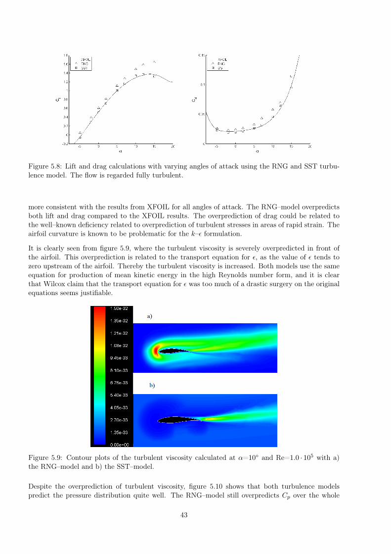
Figure 5.8: Lift and drag calculations with varying angles of attack using the RNG and SST turbu-lence model. The flow is regarded fully turbulent.
more consistent with the results from XFOIL for all angles of attack. The RNG–model overpredictsboth lift and drag compared to the XFOIL results. The overprediction of drag could be related tothe well–known deficiency related to overprediction of turbulent stresses in areas of rapid strain. Theairfoil curvature is known to be problematic for the k–ε formulation.
It is clearly seen from figure 5.9, where the turbulent viscosity is severely overpredicted in front ofthe airfoil. This overprediction is related to the transport equation for ε, as the value of ε tends tozero upstream of the airfoil. Thereby the turbulent viscosity is increased. Both models use the sameequation for production of mean kinetic energy in the high Reynolds number form, and it is clearthat Wilcox claim that the transport equation for ε was too much of a drastic surgery on the originalequations seems justifiable.
Figure 5.9: Contour plots of the turbulent viscosity calculated at α=10◦ and Re=1.0 · 105 with a)the RNG–model and b) the SST–model.
Despite the overprediction of turbulent viscosity, figure 5.10 shows that both turbulence modelspredict the pressure distribution quite well. The RNG–model still overpredicts Cp over the whole
43
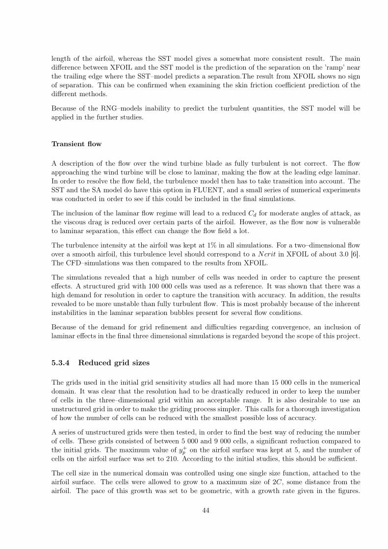
length of the airfoil, whereas the SST model gives a somewhat more consistent result. The maindifference between XFOIL and the SST model is the prediction of the separation on the ’ramp’ nearthe trailing edge where the SST–model predicts a separation.The result from XFOIL shows no signof separation. This can be confirmed when examining the skin friction coefficient prediction of thedifferent methods.
Because of the RNG–models inability to predict the turbulent quantities, the SST model will beapplied in the further studies.
Transient flow
A description of the flow over the wind turbine blade as fully turbulent is not correct. The flowapproaching the wind turbine will be close to laminar, making the flow at the leading edge laminar.In order to resolve the flow field, the turbulence model then has to take transition into account. TheSST and the SA model do have this option in FLUENT, and a small series of numerical experimentswas conducted in order to see if this could be included in the final simulations.
The inclusion of the laminar flow regime will lead to a reduced Cd for moderate angles of attack, asthe viscous drag is reduced over certain parts of the airfoil. However, as the flow now is vulnerableto laminar separation, this effect can change the flow field a lot.
The turbulence intensity at the airfoil was kept at 1% in all simulations. For a two–dimensional flowover a smooth airfoil, this turbulence level should correspond to a Ncrit in XFOIL of about 3.0 [6].The CFD–simulations was then compared to the results from XFOIL.
The simulations revealed that a high number of cells was needed in order to capture the presenteffects. A structured grid with 100 000 cells was used as a reference. It was shown that there was ahigh demand for resolution in order to capture the transition with accuracy. In addition, the resultsrevealed to be more unstable than fully turbulent flow. This is most probably because of the inherentinstabilities in the laminar separation bubbles present for several flow conditions.
Because of the demand for grid refinement and difficulties regarding convergence, an inclusion oflaminar effects in the final three dimensional simulations is regarded beyond the scope of this project.
5.3.4 Reduced grid sizes
The grids used in the initial grid sensitivity studies all had more than 15 000 cells in the numericaldomain. It was clear that the resolution had to be drastically reduced in order to keep the numberof cells in the three–dimensional grid within an acceptable range. It is also desirable to use anunstructured grid in order to make the griding process simpler. This calls for a thorough investigationof how the number of cells can be reduced with the smallest possible loss of accuracy.
A series of unstructured grids were then tested, in order to find the best way of reducing the numberof cells. These grids consisted of between 5 000 and 9 000 cells, a significant reduction compared tothe initial grids. The maximum value of y+
p on the airfoil surface was kept at 5, and the number ofcells on the airfoil surface was set to 210. According to the initial studies, this should be sufficient.
The cell size in the numerical domain was controlled using one single size function, attached to theairfoil surface. The cells were allowed to grow to a maximum size of 2C, some distance from theairfoil. The pace of this growth was set to be geometric, with a growth rate given in the figures.
44

Three of the grids from the initial study has been included in the figures. This has been done toquantify the loss of accuracy introduced by reducing the number of cells.
Three different grid parameters were investigated: (1) the effect of reducing the number of cells in thestructured boundary layer grid. (2) the effect of reducing the height of the structured boundary layergrid, and (3) the effect of changing the geometric growth rate in the rest of the numerical domain.
The simulations was performed at an angle of attack of 12◦, as the errors seem to grow with theangle of attack (see figure 5.8). The SST–model with a fully turbulent formulation was used, with aReynolds number of 1.0 · 105. In order to isolate the effect of one change in grid parameter, all gridparameters but one was kept constant when a new grid was created. Thereby the effect of the changeis always captured in the results. As the investigation resulted in more than 12 different grids, onlythe grid parameters of some grids are included in this report. They can be found in appendix A.5.
Figure 5.12 shows that the number of cells in the boundary layer grid can be reduced to approximately15 without substantial loss of data. However, using 20 cells could improve the results somewhat. Theheight of the structured grid is a more important parameter, as can be seen from the figure. A heightof 0.1C seems sufficient.
The geometric growth rate of the cells in the structured boundary layer is dictated by the height andthe number of cells. The results were investigated in order to see if the solution was sensitive to thisgrowth rate. No significant bias was found, indicating that the solution is not sensitive to the choiceof this parameter.
As can be seen from figure 5.13, the choice of the geometric growth rate in the external domain is acrucial parameter. It should be set as low as possible, in order to get a better prediction of the dragacting on the airfoil. The lift is not very sensitive to the resolution, as expected. However, whenkeeping BLh at 0.1C, the geometric growth rate can be increased to 1.45 before the results get asinaccurate as the BLh = 0.05C results. This indicates that increasing the boundary layer height isan efficient way of achieving accurate results with few cells.
When constructing the three dimensional grid, an effort should be made in order to get the boundarylayer height 0.1 times the longest chord length on the blade, with approximately 20 cells normal tothe surface. Then a proper growth rate will be determined, so that the total number of cells arewithin an acceptable range.
45
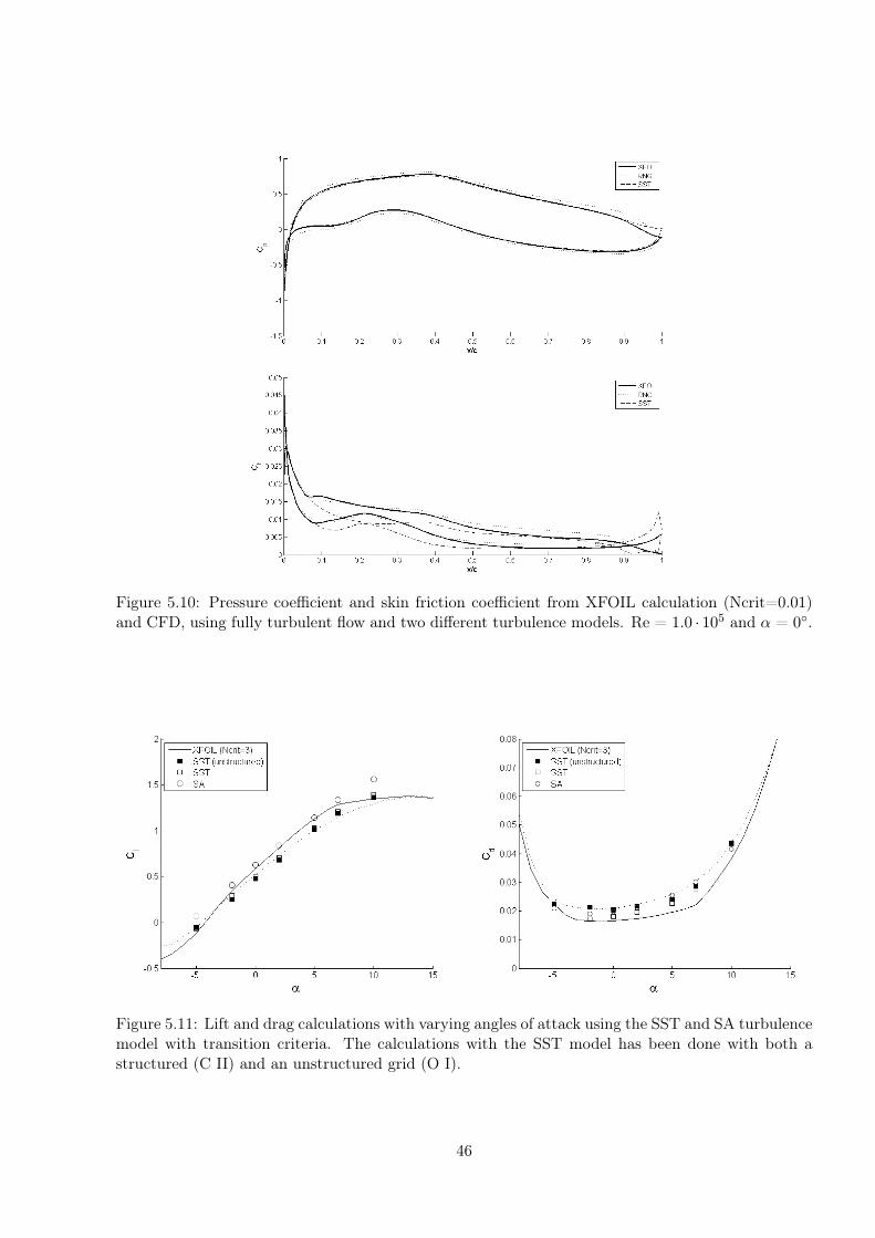
Figure 5.10: Pressure coefficient and skin friction coefficient from XFOIL calculation (Ncrit=0.01)and CFD, using fully turbulent flow and two different turbulence models. Re = 1.0 · 105 and α = 0◦.
Figure 5.11: Lift and drag calculations with varying angles of attack using the SST and SA turbulencemodel with transition criteria. The calculations with the SST model has been done with both astructured (C II) and an unstructured grid (O I).
46

Figure 5.12: Numerical simulation results with varying number of cells in the structured boundarylayer (BL) grid. Three results from the initial simulation with a refined grid is also included. Thesimulations are done with Re = 1.0 · 105, TI = 1.0% and α = 12◦.
Figure 5.13: Numerical simulation results with varying geometrical growth rates in the externaldomain. The extended use of size functions makes the ’refined grids’ better than the ones testedhere. However, the number of cells i one third in the new cases.
47
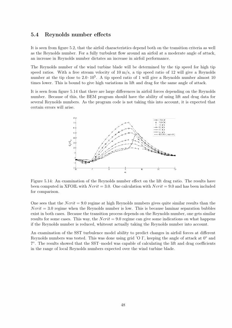
5.4 Reynolds number effects
It is seen from figure 5.2, that the airfoil characteristics depend both on the transition criteria as wellas the Reynolds number. For a fully turbulent flow around an airfoil at a moderate angle of attack,an increase in Reynolds number dictates an increase in airfoil performance.
The Reynolds number of the wind turbine blade will be determined by the tip speed for high tipspeed ratios. With a free stream velocity of 10 m/s, a tip speed ratio of 12 will give a Reynoldsnumber at the tip close to 2.0 · 105. A tip speed ratio of 1 will give a Reynolds number almost 10times lower. This is bound to give high variations in lift and drag for the same angle of attack.
It is seen from figure 5.14 that there are large differences in airfoil forces depending on the Reynoldsnumber. Because of this, the BEM program should have the ability of using lift and drag data forseveral Reynolds numbers. As the program code is not taking this into account, it is expected thatcertain errors will arise.
Figure 5.14: An examination of the Reynolds number effect on the lift drag ratio. The results havebeen computed in XFOIL with Ncrit = 3.0. One calculation with Ncrit = 9.0 and has been includedfor comparison.
One sees that the Ncrit = 9.0 regime at high Reynolds numbers gives quite similar results than theNcrit = 3.0 regime when the Reynolds number is low. This is because laminar separation bubblesexist in both cases. Because the transition process depends on the Reynolds number, one gets similarresults for some cases. This way, the Ncrit = 9.0 regime can give some indications on what happensif the Reynolds number is reduced, whiteout actually taking the Reynolds number into account.
An examination of the SST turbulence model ability to predict changes in airfoil forces at differentReynolds numbers was tested. This was done using grid ’O I’, keeping the angle of attack at 0◦ and7◦. The results showed that the SST–model was capable of calculating the lift and drag coefficientsin the range of local Reynolds numbers expected over the wind turbine blade.
48
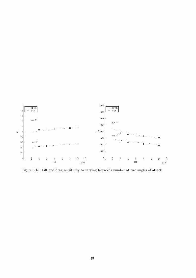
Figure 5.15: Lift and drag sensitivity to varying Reynolds number at two angles of attack.
49

5.5 Recommendations for 3D simulations
Based on the experience gained from the 2D–simulations, a rough estimate for some of the simulationparameters in the 3D case can be determined.
For the three dimensional grid, the following guidelines should be followed:
• 200 or more grid–points around the airfoil in the chordwise direction
• Increased chordwise refinement close to the leading and trailing edge
• A maximum value of y+p no more than 5, and an average value no more than 1.
• At least 15 cells in the structured boundary layer grid
• A thickness of the structured boundary layer grid no less than 0.1C
• The geometrical growth rate outside the boundary layer grid should be as low as possible
In addition, the k–ω SST–model should be used in its fully turbulent form.
50

Chapter 6
Construction of 3D model
6.1 3D model
A 3D model of the wind turbine blades was obtained from the company that machined the blades.This way it was assured that the model used in the numerical simulations was the exact same as theone used for the production of the blades. The uncertainty in the 3D model is then only related tothe error in the production process, which can be assumed to be small.
The hub was measured manually and added to the model of the 3D blades. The uncertaintiesintroduced in this process can be expected to be somewhat larger than in the modelling of theblades. However, the hub is not a vital part of the model, and small uncertainties can be acceptedhere.
Figure 6.1: A 3D model of the wind turbine blades and hub. The different parts of the model aredenoted
As long as the tower influence is excluded from the model, and the wind tunnel modelled as a circular
51

tube, the flow field around the wind turbine can be assumed to be be rotationally periodic. Thismakes it possible to model only one third of the complete model, as the flow in the other two thirdswill be fully described by the flow in the first. This reduces the needed number of cells to one–third,making it more easy to reduce the number of cells needed.
Figure 6.2: The numerical domain. The wind tunnel is modelled as one third of a cylinder. Theperiodic boundary surface grid has been excluded from the wiev. The wind tunnel blade and hubcan be seen in white inside the model.
The wind tunnel was modelled as a cylinder with a cross section equal to that of the real wind tunnel.The cross section of the wind tunnel is 2.7 m · 1.9 m, making the corresponding radius 1.278 m. Thisapproximation is done in order to reduce the need for sliding meshes. The procedure has been usedin other studies, and has been reported not to introduce significant errors [21].
No mesh indepency test was made, as this is very expensive in 3D. But based on the two–dimensionalstudies, good choices of grid parameters is expected to reduce numerical errors to a minimum.
6.2 Surface mesh
6.2.1 Blade
The surface mesh was created using GAMBIT. The blade needs a high degree of refinement. Becauseof this a structured mesh was chosen in order to reduce the amount of cells needed to get a fineresolution near the leading and trailing edge. A total of 300 nodes was used around the airfoil inthe chordwise direction, and 200 nodes in the spanwise direction. Close to the root and the tip, thespanwise extension of the cells was kept at 0.1 mm. Near the leading and trailing edge, the chordwiseextension of the cells was kept at 0.03 mm close to the tip, and 0.1 mm close to the root.
In total, 60 000 faces was used to describe the surface of the blade.
52

6.2.2 Tip
An unstructured mesh was used to represent the tip of the wing. The elements had a size correspond-ing to the streamwise extension of the cells close to the tip on the blade surface, but was allowed togrow somewhat toward the center of the tip surface.
A total of 3056 faces was used to describe the tip of the blade.
Figure 6.3: Detail of grid at the tip of the turbine blade.
6.2.3 Junction
The junction between the blade and the hub consists of two parts. A cylindrical section close to thehub, and a transition from this cylinder to the blade. Due to the three dimensional curvature of thelatter section, an unstructured mesh was chosen. The size of the element edges was kept below 1 mmin the transition part of the blade, and below 0.5 mm on the tubular section.
A total number of 28 500 faces was used to describe this part of the blade.
6.2.4 Hub
The hub is formed as a cylinder with a rounded front and rear. An unstructured grid was usedhere as well. The size of the face edges was set to a maximum of 7 mm on the hub surface, with arefinement in the front, near the blade junction and close to the rear of the hub.
A total number of 7500 faces was used to describe the hub.
6.2.5 Exterior surfaces
There was five exterior surfaces in the model. Two periodic boundaries, one inlet, one outlet andone surface describing the wind tunnel roof. These surfaces was all meshed using triangular faces.Far from the wind turbine, the cell edges was set to a length of 0.2 m, and size functions was usedto enhance refinement close to the wind turbine.
The mesh on the three latter surfaces can be seen in figure 6.2. The periodic boundary mesh wascreated using a size function with a geometric growth rate of 1.2, that allowed the mesh to grow from
53

Figure 6.4: Detail of the grid close to the hub. Size functions was used to refine the grid close to thejunction and near the front and rear of the hub.
the sizes related to the hub, to the sizes related to the rest of the exterior surface meshes. A figureof the periodic boundary grid can be found in appendix A.6.
6.3 Boundary layer grid
Using the program TGRID, a boundary layer grid was created on all the physical surfaces. Prismlayers were grown from all wall surfaces (blade, tip, junction, hub). A layer of pyramid cells wasattached to the surface of the structured cell faces on the boundary layer grid. This was done inorder to be able to use an unstructured volume grid in the rest of the domain.
The viscous shear on the wind turbine surface is expected to be more or less the same in the 3Dcase as in the 2D simulations, as long as the local Reynolds number is the same. The shear couldbe influenced by three–dimensional effects, but these are expected to occur at low tip speed ratioswhere the blade Reynolds number is allready low. The 2D simulations showed that as long asyp < 5 · 10−4C, the corresponding value of y+
p was low enough to resolve the viscous boundary layerin a decent way. Based on the tip chord length of 26 mm, the grid point closest to the blade surfaceshould be approximately 0.01 mm from the wall. Closer to the hub, the local Reynolds number isexpected to decrease (as seen in figure 7.1), a fact that indicates that the choice of yp should be basedon the tip conditions.
The boundary layer thickness should be kept higher than 0.1C. Based on the maximum chord–length,the boundary layer grid thickness should be approximately 9 mm.
23 cells were created in the boundary layer grid, with a geometric growth rate of 1.2, yielding aboundary layer grid height of 3.3 mm. The program was incapable of creating a higher grid, becauseof the proximity of the faces, and the concave curvature of the blade pressure side. This resulted ina boundary layer height less than one third the recommended value, a possible cause of numericalstability problems in cases where the root of the blade is stalled.
54
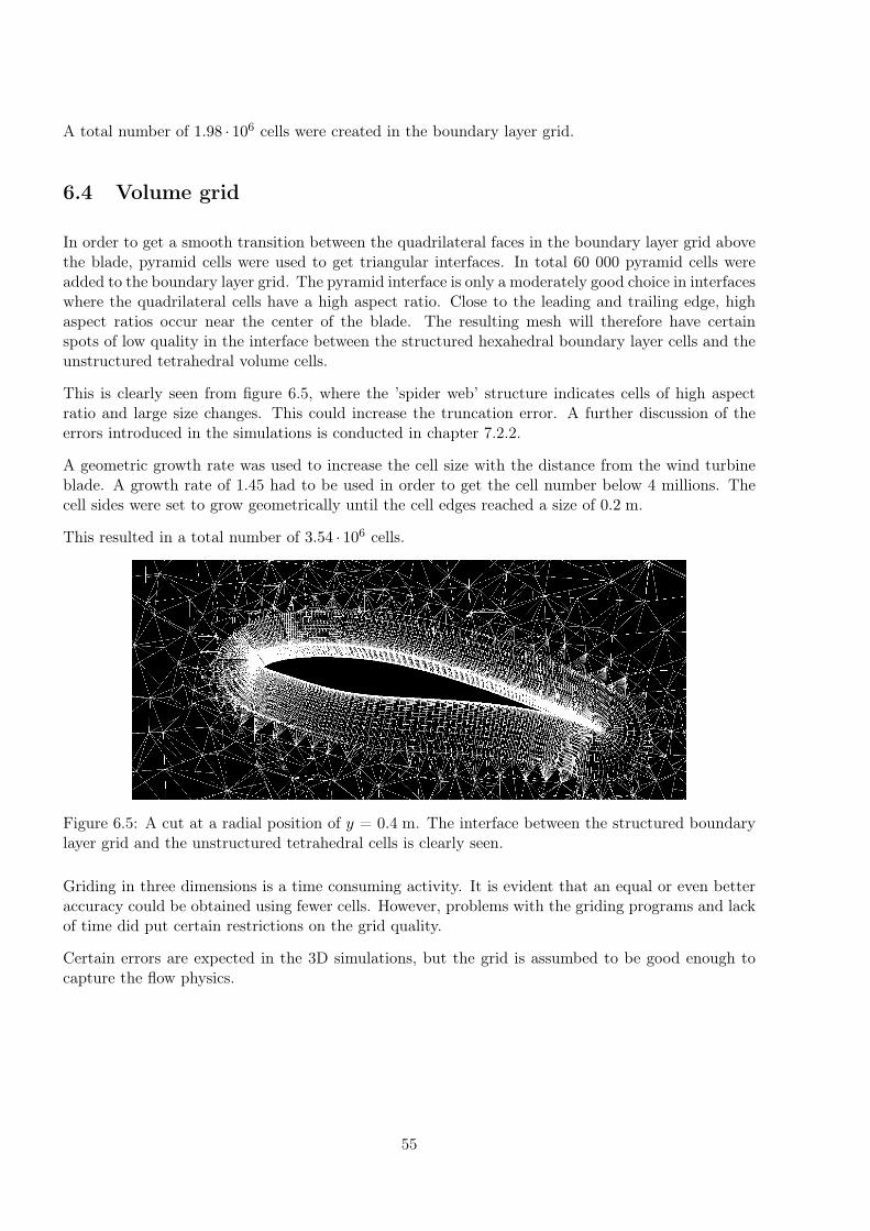
A total number of 1.98 · 106 cells were created in the boundary layer grid.
6.4 Volume grid
In order to get a smooth transition between the quadrilateral faces in the boundary layer grid abovethe blade, pyramid cells were used to get triangular interfaces. In total 60 000 pyramid cells wereadded to the boundary layer grid. The pyramid interface is only a moderately good choice in interfaceswhere the quadrilateral cells have a high aspect ratio. Close to the leading and trailing edge, highaspect ratios occur near the center of the blade. The resulting mesh will therefore have certainspots of low quality in the interface between the structured hexahedral boundary layer cells and theunstructured tetrahedral volume cells.
This is clearly seen from figure 6.5, where the ’spider web’ structure indicates cells of high aspectratio and large size changes. This could increase the truncation error. A further discussion of theerrors introduced in the simulations is conducted in chapter 7.2.2.
A geometric growth rate was used to increase the cell size with the distance from the wind turbineblade. A growth rate of 1.45 had to be used in order to get the cell number below 4 millions. Thecell sides were set to grow geometrically until the cell edges reached a size of 0.2 m.
This resulted in a total number of 3.54 · 106 cells.
Figure 6.5: A cut at a radial position of y = 0.4 m. The interface between the structured boundarylayer grid and the unstructured tetrahedral cells is clearly seen.
Griding in three dimensions is a time consuming activity. It is evident that an equal or even betteraccuracy could be obtained using fewer cells. However, problems with the griding programs and lackof time did put certain restrictions on the grid quality.
Certain errors are expected in the 3D simulations, but the grid is assumbed to be good enough tocapture the flow physics.
55

56

Chapter 7
Results and discussion
7.1 BEM results
7.1.1 BEM calculation procedure
A Blade Element Momentum computation of the wind turbine performance was made. This wasdone using the PERFORMANCE code that is described in figure 3.7. The blade geometry wasobtained from the 3D CAD model, that was the basis of both the production of the wind turbineblades, and the CFD model. However, in order to make the format acceptable for the BEM code,some minor changes had to be made to the blade junction. The description of the blade geometrycan be found in appendix A.3. Lift and drag curves obtained in the two–dimensional study was usedin the calculations.
For high tip speed ratios the BEM code had convergence problems for certain blade elements closeto the root of the blade. This seems to occur in cases where the wind turbine acts as a propeller,adding energy to the wind. In these cases the axial induction factor and the blade section momentwill become negative.
7.1.2 Blade section Reynolds number
The program code can only apply one lift and drag curves at the time. Because of this, a fixedReynolds number is used in the calculations. This is inaccurate, as the Reynolds number is knownto vary with the rotational speed of the wind turbine. An initial study was therefore conducted,in order to calculate blade Reynolds number and angle of attack for different tip speed ratios. TheNcrit = 3.0 results with a fixed Reynolds number of 1.0 · 105 was used in the calculations. The axialand angular induction factors were then found, making it possible to determine the local flow angle(ϕ). This was used to determine the angle of attack, using equation 3.15 and the following relation:
α = ϕ− θ (7.1)
The Reynolds number was found using the relative velocity (Urel) and the local chord length (C)1.The relative velocity was derived from the induction factors, using equation 3.14. The results are
1The local Reynolds number was calculated using a kinematic viscosity of 1.46 · 10−5 m2/s
57

presented in figure 7.1, and form a basis of the following discussion, where local angles of attack andReynolds numbers are important parameters.
Figure 7.1: Variations of Re and α over the blade, for λ = 2, 3, 4, 5, 6, 7, 8, 9, and 10. Ncrit = 3.0.The angle of attack is gradually reduced, and the Reynolds number increased with increasing tipspeed ratios.
The Reynolds number is found to vary from approximately 3.0 · 104 to a maximum value of almost2.0 · 105. From the findings in chapter 5.4, it is clear that this will affect the lift and drag coefficientsof the airfoil. The lift and drag curves used in the further study have been calculated at a Reynoldsnumber of 1.0 · 105. This has been chosen as it is representative for the design conditions of the windturbine (5 < λ < 7). In order to get a more accurate result from the BEM calculations, lift and dragcurves for different Reynolds number should have been applied. But, as the program is not designedfor that, this will not be taken into account.
The Reynolds number study in chapter 5.4 indicated that the angle where stall occurred did notchange much with the Reynolds numbers. This means that these results could give good indicationsof when the wind turbine blade will stall. The results presented in figure 7.1 indicate that the bladewill be fully stalled for tip speed ratios below 4, whereas it will be partly stalled at a tip speed ratioof 4. Increasing the tip speed ratio above 5, the the boundary layer on the wind turbine can beexpected to remain attached for tip speed ratios up to 10. However, some separation will probablyoccur on the separation trap near the trailing edge. For high tip speed ratios, the angle of attack isreduced towards −5◦. However, it is hard to say whether or not the root of the blade is stalled forhigh tip speed ratios, as the BEM code gave no solutions for these conditions.
7.1.3 CP and CT calculations
Power curve predictions
Using the BEM method, CP and CT curves was calculated for tip speed ratios ranging from λ = 1 toλ = 25. Some convergence problems did occur for blade elements close to the hub for high tip speedratios, but the effect is small for all tip speed ratios below 9 2. The results from the calculations arepresented in figure 7.2
2A more detailed study of the blade forces is found in chapter 7.3
58
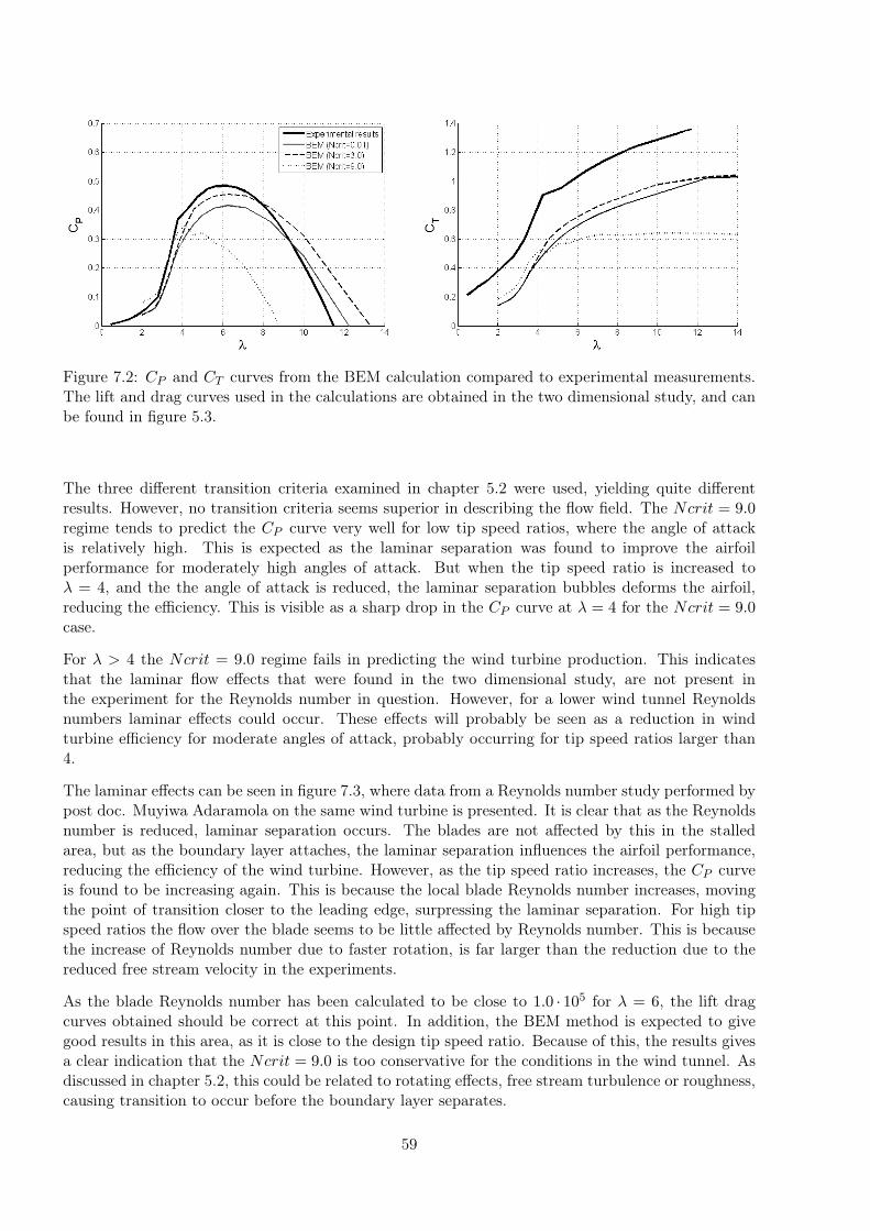
Figure 7.2: CP and CT curves from the BEM calculation compared to experimental measurements.The lift and drag curves used in the calculations are obtained in the two dimensional study, and canbe found in figure 5.3.
The three different transition criteria examined in chapter 5.2 were used, yielding quite differentresults. However, no transition criteria seems superior in describing the flow field. The Ncrit = 9.0regime tends to predict the CP curve very well for low tip speed ratios, where the angle of attackis relatively high. This is expected as the laminar separation was found to improve the airfoilperformance for moderately high angles of attack. But when the tip speed ratio is increased toλ = 4, and the the angle of attack is reduced, the laminar separation bubbles deforms the airfoil,reducing the efficiency. This is visible as a sharp drop in the CP curve at λ = 4 for the Ncrit = 9.0case.
For λ > 4 the Ncrit = 9.0 regime fails in predicting the wind turbine production. This indicatesthat the laminar flow effects that were found in the two dimensional study, are not present inthe experiment for the Reynolds number in question. However, for a lower wind tunnel Reynoldsnumbers laminar effects could occur. These effects will probably be seen as a reduction in windturbine efficiency for moderate angles of attack, probably occurring for tip speed ratios larger than4.
The laminar effects can be seen in figure 7.3, where data from a Reynolds number study performed bypost doc. Muyiwa Adaramola on the same wind turbine is presented. It is clear that as the Reynoldsnumber is reduced, laminar separation occurs. The blades are not affected by this in the stalledarea, but as the boundary layer attaches, the laminar separation influences the airfoil performance,reducing the efficiency of the wind turbine. However, as the tip speed ratio increases, the CP curveis found to be increasing again. This is because the local blade Reynolds number increases, movingthe point of transition closer to the leading edge, surpressing the laminar separation. For high tipspeed ratios the flow over the blade seems to be little affected by Reynolds number. This is becausethe increase of Reynolds number due to faster rotation, is far larger than the reduction due to thereduced free stream velocity in the experiments.
As the blade Reynolds number has been calculated to be close to 1.0 · 105 for λ = 6, the lift dragcurves obtained should be correct at this point. In addition, the BEM method is expected to givegood results in this area, as it is close to the design tip speed ratio. Because of this, the results givesa clear indication that the Ncrit = 9.0 is too conservative for the conditions in the wind tunnel. Asdiscussed in chapter 5.2, this could be related to rotating effects, free stream turbulence or roughness,causing transition to occur before the boundary layer separates.
59
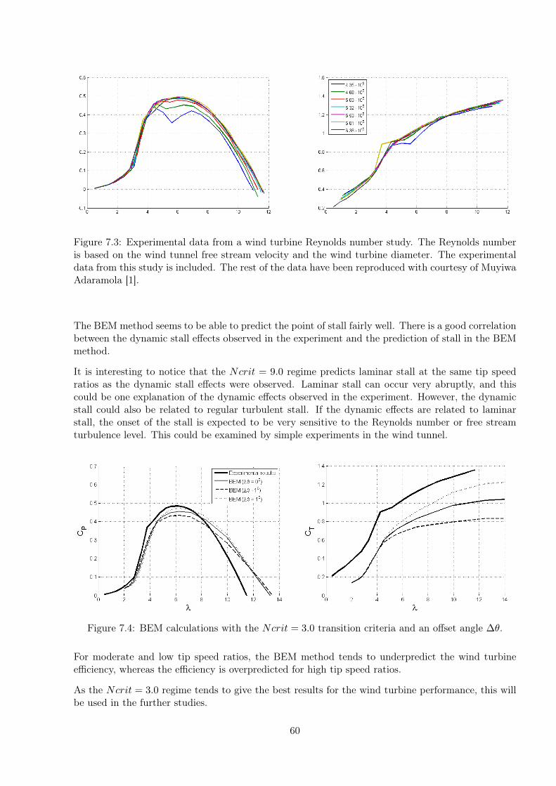
Figure 7.3: Experimental data from a wind turbine Reynolds number study. The Reynolds numberis based on the wind tunnel free stream velocity and the wind turbine diameter. The experimentaldata from this study is included. The rest of the data have been reproduced with courtesy of MuyiwaAdaramola [1].
The BEM method seems to be able to predict the point of stall fairly well. There is a good correlationbetween the dynamic stall effects observed in the experiment and the prediction of stall in the BEMmethod.
It is interesting to notice that the Ncrit = 9.0 regime predicts laminar stall at the same tip speedratios as the dynamic stall effects were observed. Laminar stall can occur very abruptly, and thiscould be one explanation of the dynamic effects observed in the experiment. However, the dynamicstall could also be related to regular turbulent stall. If the dynamic effects are related to laminarstall, the onset of the stall is expected to be very sensitive to the Reynolds number or free streamturbulence level. This could be examined by simple experiments in the wind tunnel.
Figure 7.4: BEM calculations with the Ncrit = 3.0 transition criteria and an offset angle ∆θ.
For moderate and low tip speed ratios, the BEM method tends to underpredict the wind turbineefficiency, whereas the efficiency is overpredicted for high tip speed ratios.
As the Ncrit = 3.0 regime tends to give the best results for the wind turbine performance, this willbe used in the further studies.
60

Thrust curve calculations
While the predictions of the power coefficient were rather accurate, there are larger deviances in thethrust coefficient predictions. However, the difference seems to be rather constant. It is also clearthat Glauerts correction factor succeeds in predicting thrust in the invalid area (a >> 0.2).
However, the constant underprediction of the thrust force needs to be commented upon. One possiblesource of uncertainty is the blade pitch angle. It was possible to pitch the blade in the experimentalsetup. If the blades were misaligned, they could add bias to the results. This was tested by introduc-ing an offset angle in the BEM calculations. An offset angle of 1◦ was chosen, as the uncertainties inthe experimental pitch alignment are expected to be below this value.
As indicated in figure 7.4, even a small offset angle can cause large changes in the CT curve forhigh tip speed ratios. However, for λ = 5 the differences are small. Because of this the thrustcoefficients should be compared at the design tip speed ratio. Here the Reynolds number is correct,two dimensional effects are assumed to be small, and an errenous offset angle in the experiment willhave little impact on the results.
The underprediction of the thrust force seems to be in the order of ∆CT ≈ 0.3, where ∆CT =CT,exp − CT,bem.
The experimental thrust coefficient includes the thrust (drag) caused by the tower, hub and trans-mission belt behind the wind turbine. It is probable that the tower thrust is dominant comparedto the other sources of drag. It is then possible to determine a tower thrust coefficient that containthe additional drag. If this coefficient is in the order of what is expected for a circular cylinder, therotor thrust coefficient can be assumed to be correct. If the tower thrust coefficient is too large, thenthe BEM thrust calculations are probably too low. If one assumes that the disk thrust is correctlypredicted by the BEM method, the tower thrust will be given by:
Texp = Tbem + Ttower
CT,exp − CT,bem =Ttower
12ρU∞Arotor
∆CT = CT,towerAtowerArotor
(7.2)
The total thrust coefficient and the rotor thrust coefficient are both based on the rotor area. Weknow that the frontal area of the tower is approximately 0.052 m2. Introducing the known ∆CT intoequation 7.2, we get CTtower ≈ 3.7. This is far higher than what can be expected from the cylindricaltower only. A circular cylinder can be expected to have a drag coefficient no higher than 1.2 in therange of Reynolds numbers expected here [27]. The other sources of thrust are not expected to belarger than twice the thrust of the tower. This is an indication that the BEM method underpredictsthe thrust force.
61

7.2 CFD results
7.2.1 CFD solution strategy
The Navier–Stokes solver, FLUENT, was used for the CFD simulations. FLUENT uses a finitevolume method, and steady–state calculations of the RANS equations was performed. The flowregime was assumed to be incompressible, as the velocity in the study was below Mach 0.3 for all tipspeed ratios except the λ = 11 case. In this case the tip speed do actually reach 110 m/s, but this isan exception, not representative for the majority of the cases studied. Compressibility effects weretherefore excluded from this study.
The SIMPLEC algorithm was used to couple the pressure and velocity fields. The computations wererun on a 64–bit computer with four processors, making parallel processing possible. The turbulenteddy viscosity was modeled using the k–ω SST–model. The momentum equations were solved using aquadratic discretisation scheme (QUICK) for the convective terms, while the pressure was discretisedusing a normal 1. order discretisation scheme. This was done to enhance convergence, as higher orderschemes of pressure discretisation showed to be unstable. Under–relaxation factors was tuned duringthe iteration process, in order to achieve a converged solution.
A total number of 5000 iterations showed to be sufficient for most calculations, taking approximately24h to complete.
The viscosity was set to 1.7894 · 10−5 kg/m · s, and the density to 1.225 kg/m3. The inlet velocitywas set to 10 m/s, which gave a Reynolds number based on the wind turbine diameter of 6.16 · 105.This was done before the experiments was performed, resulting in a Reynolds number approximately3.4% lower than in the experiments. As seen in figure 7.3 this is not expected to have any significanteffect on the solution. However, if transition effects were to be modelled, the flow regime would bemore sensitive to Reynolds number effects.
At the inlet a turbulence intensity and a turbulent viscosity ratio was determined. The turbulenceintensity is described in equation 3.49, and was set to 1.5% at the inlet. A turbulent viscosity ratioof 10 was set at the inlet, in order to keep ε ≈ 2k. This gave a turbulence intensity of approximately0.5% at the wind turbine position in an empty wind tunnel.
7.2.2 Error analysis
According to the AIAA guidelines for verification and validation of CFD analysis, error is definedas: "A recognizable deficiency in any phase or activity of modeling and simulation that is not due tolack of knowledge". An uncertainty is defined as: "A potential deficiency in any phase or activityof the modeling process that is due to the lack of knowledge" [2]. There are several sources of errorsand uncertainties in this analysis. Some of the uncertainties are allready commented upon. In thissection the errors in the CFD analysis will be addressed.
Physical approximation errors
There are several physical approximation errors in the model. The most important ones are theassumptions of the flow regime as stationary, turbulent and rotationally periodic. The assumption ofrotational periodicity means that the tower had to be excluded from the model, and that the windtunnel had to be modeled as a circular cylinder.
62

The assumption of a stationary flow regime excludes all dynamic effects. As severe dynamic effectswere observed in the experiments, this omission do affect the results to a large extent. The assumptionof a fully turbulent regime do exclude all laminar effects. As indicated in chapter 7.1.3, laminar effectscould be important in prediction of the dynamic stall occurring at moderate and low tip speed ratios.However, for other tip speed ratios examined, laminar effects are expected to play a less importantrole.
The boundary layer close to the wind tunnel wall was removed in order to reduce the demand forcells. Consequently, the wind tunnel walls were modeled using a no–shear condition.
Computer round off errors
In order to reduce the computer round off errors, the ’double precision solver’ was used in all sim-ulations. Because of this, computer round off errors can be assumed to be very small compared toother errors in the model.
Iterative convergence error
The iterating process was run until no significant drop in residual was observed. For some tip speedratios there were still some variations or oscillations in the solution at this point. This is denotediterative convergence error. In order to reduce this error, the moment and thrust force was observed.For cases where the variations in these forces were less than 1%, a converged solution was assumed.An illustration of iterative convergence errors can be seen as small oscillations in the Cm and Cdcurves in appendix A.8.
Discretization error
No grid dependence test was made in the three dimensional case, as this is very time consuming.Based on the two dimensional analyses made in chapter 5.3, the constructed grid was assumed tobe good enough for the simulations. However, the discussion in chapter 6.4 revealed that the con-structed grid has certain shortcomings. Especially in the interface between the structured hexahedralboundary layer cells and the tetrahedral cells in the rest of the numerical domain. In addition, theheight of the structured boundary layer grid close to the root of the blade was much lower than whatwas recommended in the 2D simulations. The low grid quality in these parts of the domain couldlead to rather large truncation errors for certain cases.
The discretization errors are reduced to some extent by introducing the QUICK discretization scheme.
For tip speed ratios 9 and 11, completely converged solutions were hard to achieve. In order to getstable solutions, the discretisation had to be reduced to a 1. order upwind scheme. The instabilityobserved could be caused by inherent instabilities in the flow, e.g vortex shedding from the blade. Itis also plausible that the instability of the solution is connected to the reduced grid refinement closeto the root of the blade. A better grid might improve the results. The values of y+
p was not found toexceed the recomended values, as illustrated by figures in appendix A.7.
It is expected that the physical approximation errors and the discretisation errors will be the dominantsources of errors in the simulations.
63

7.2.3 CP and CT calculations
From figure 7.5 it is evident that the CP curve is reproduced by the CFD simulations. The differencesbetween measured and simulated power coefficients were lower than 5% for tip speed ratios up to 6.The differences were somewhat larger for higher tip speed ratios. This could be related to truncationerrors introduced by reduction of the discretisation scheme.
For low tip speed ratios there is a very good agreement between the experimental results and thesimulations. The dynamic stall effects found in the experiment were not observed. Stationarysolutions for λ = 4 and 5 were obtained, and they tended to be quite stable. This is an indicationthat they are related to laminar effects as the dynamic stall was not captured in these fully turbulentsimulations.
Figure 7.5: CP and CT curves from the CFD simulation compared to experimental measurements.The Ncrit = 3.0 BEM calculation has been included.
For the CFD simulations, the mean difference between the measured and simulated thrust coefficientis approximately ∆CT ≈ 0.13. Using equation 7.2, this corresponds to a tower thrust coefficientCTtower ≈ 1.6. This is somewhat larger than expected for an infinite cylinder immersed in laminarflow [27].
It is hard to say whether the flow around the tower will be laminar or turbulent. The Reynoldsnumber based on the diameter of the tower and a free stream velocity of 10 m/s is varying between3 · 105 and 7 · 105, depending on the tower diameter. This is in the range of Reynolds numbers wheretransition is known to occur (see figure A.8 in the appendix [27]). However, as the cylinder has anon–uniform diameter, it will probably have a drag relationship like a cylinder of finite span. Thusthe drag coefficient of the tower alone should be lower than 1.2.
The blocking effect caused by the rotor will also influence the tower drag coefficient, as it is scaledby the free stream velocity. This could lead to a reduction in ∆CT in cases where the blocking effectis more dominant. This is not found in the experiments, as ∆CT is seen to be high for moderate tipspeed ratios. For these conditions the blocking is expected to be quite uniform and high, as muchenergy is extracted from the free stream. As one sees from figure 7.6, the blocking effect causes awind speed reduction up to 30% at the tower position when λ = 6.
It must also be noted that the presence of the tower will induce an upstream blocking effect, reducingthe free stream velocity in the rotor plane. This will also affect the measured thrust force.
64

Figure 7.6: Contour plot of the axial speed distribution in a plane z=0 at λ = 6. One wind turbineblade has been excluded from the view.
In total, the thrust deficit found in the CFD simulations can be said to be within the expected range.The influence of the thrust forces will increase the tower drag coefficient. And as the power curve iswell described using the CFD method, it can be expected that the actual thrust forces acting on therotor and hub are fairly well described as well.
Experimental testing of the tower drag could have been performed by removing the blades from theturbine. This has not been done.
The CFD calculations have given a good estimate of both the thrust and power prediction of thewind turbine. There is a good match between the experimental results and the simulations. TheBEM method did give reasonable results for the power curve, but the thrust forces tended to beunderpredicted. This underprediction is not caused by the hub drag. This drag is not included inthe BEM calculations, but according to CFD results for λ = 4, less than 2% of the the drag on themodelled geometry is caused by forces acting on the the hub. It is therefore clear that the BEMmethod underpredicts the thrust forces.
65

7.3 Blade forces
7.3.1 Methods
When comparing CP and CT curves, only the gross forces acting on the blade are examined. Agood representation of the power or thrust coefficient is therefore no proof that the spanwise forcedistribution is well described. Because of this a more detailed study of the forces acting on thedifferent blade sections was conducted. The forces acting on each blade element was extracted bythe BEM code. The spanwise force distribution was found using equation 3.22 and 3.23. Thecomputations were made for five different tip speed ratios. In order to reduce the inaccuracies, liftand drag curves for the corresponding Reynolds number were used. For λ = 3 and 4 a Reynoldsnumber of 40 000 was used. For λ = 6 a Reynold number of 100 000 was used, while a Reynoldsnumber of 150 000 was used for λ = 9 and 11.
Data from the CFD simulations was extracted from FLUENT by creating 60 iso–surfaces with dif-ferent radial distances from the centerline. From all blade cell faces intersected by one of theseiso–surfaces, the total pressure and viscous wall shear stress vector at the cell center was extracted.In addition the cell face normal vector and area of each cell was computed. These data was usedto extract both axial (thrust) and tangential (moment) forces acting on the different sections of theblade. The forces are denoted dFx and dFz and are given in [N/m ]. They were determined by addingall viscous and pressure forces acting on the wall cell faces in one radial section of the wind turbineblade:
dFx =C
Atot
j=N∑j=0
pj(Ax)j + (τw,x)jAj (7.3)
dFz =C
Atot
j=N∑j=0
pj(Az)j + (τw,z)jAj (7.4)
(Ai)j is the total area of cell face j multiplied by the cell face normal vector component in directionxi. There are N cells in one radial section. pj and (τi)j are the total pressure in cell j and the viscouswall shear acting on the same cell in the xi direction. All cells in one radial section do have the sameheight (or spanwise extension). Therefore this simplified method is applicable.
Atot is the sum of the area of all cell faces in one radial section, and C is the local chordlength. Bydividing the sum by the ’height’ of the radial section (Atot/C), the forces are made independent ofthe cell faces area.
Integrated along the blade we get the total thrust force in the axial direction, T , and the totalmoment in the tangential direction, M .
T =∫ R
0dFxdr
M =∫ R
0dFzrdr
66

7.3.2 Results
From figure 7.7, one sees how the blade element method manages to predict tangential forces for λ ≥ 6fairly well. Both the magnitude and spanwise variations are captured. The fact that the spanwisevariations near the tip are well–described, indicates that Prandtls tip loss succeeds in quantifyingthe loss of circulation at the tip of the blade.
For λ = 4, the tip effect is not properly described. The reductions in blade forces start too early andare decreasing too slow compared to the CFD results.
Looking at the blade thrust forces, the tip effect is well described for λ ≤ 6. However, for λ = 9 and11 the rate of which the axial induction factor is increasing toward one, as one approaches the tip ofthe blade, is too low to capture the tip effect.
It is clear that the thrust force is systematically underpredicted by BEM method. The results wassomewhat improved by using the correct Reynolds number in the calculations, but underpredictionis still clear. This evident for all tip speed ratios.
There is generally a better accordance when looking at the tangential forces. Especially close to thedesign point there are only small differences between the two methods. The differences observed arerelated to tip and root effects. This confirms the assumption that the BEM method works well closeto the design point.
When moving away from the design tip speed ratio, the differences increase. This is expected, asthree dimensional effects are presumed to be more dominant for high an low tip speed ratios.
The tip loss effects are related to the presence of a tip vortex. However, looking at the spanwisedistribution of tangential forces, there are indications of a trailing vortex at the root as well. Thisis clearly visible when examining the tangential forces for λ = 6. In figure 7.7 a clear reduction isseen in dFz as one approaches the root of the blade. This is an indication that there is leakage ofcirculation here as well. As this effect is not described in the BEM model, this will lead to certainerrors for low radii. However, as these forces acts close to the root of the blade, they contribute littleto the total moment. As a result, these errors do not influence the CP predictions much.
It is evident when looking at figure 7.7 that even though BEM method managed to predict the CP –curve fairly well for low tip speed ratios, the actual flow physics around the blade are not captured.The spanwise variations in dFx and dFz seen in the CFD calculations for λ = 3 are not at all describedby the BEM method. These spanwise variations indicate that there are substantial spanwise pressuregradients and velocity components present in the flow field.
It is clear that there are separating effects present at this point. Both the experimental measurementsand the CFD simulations confirm that. The BEM method predicted angles of attack larger than 15◦
for all radii at λ = 3. This means that according to the BEM method, the blade should be fullystalled from root to tip at this point. However, looking at the high contribution to the moment (dFz)occurring at r/R = 0.3, the blade do not seem to be stalled at this radial position. dFz is actuallyhigher inn this case than for any of the other examined tip speed ratios. This could be an indicationthat rotational augmentation and stall delay effects are present.
67

Figure 7.7: Spanwise forces acting on the wind turbine blade for different λ. The forces has beenplotted against spanwise (radial) position, r/R. The thick line is the CFD results, while the thinnerline is BEM results using Ncrit = 3.0 and lift and drag curves for Reynolds numbers correspondingto the operating condition. The dotted line is BEM results using Ncrit = 9.0.
68
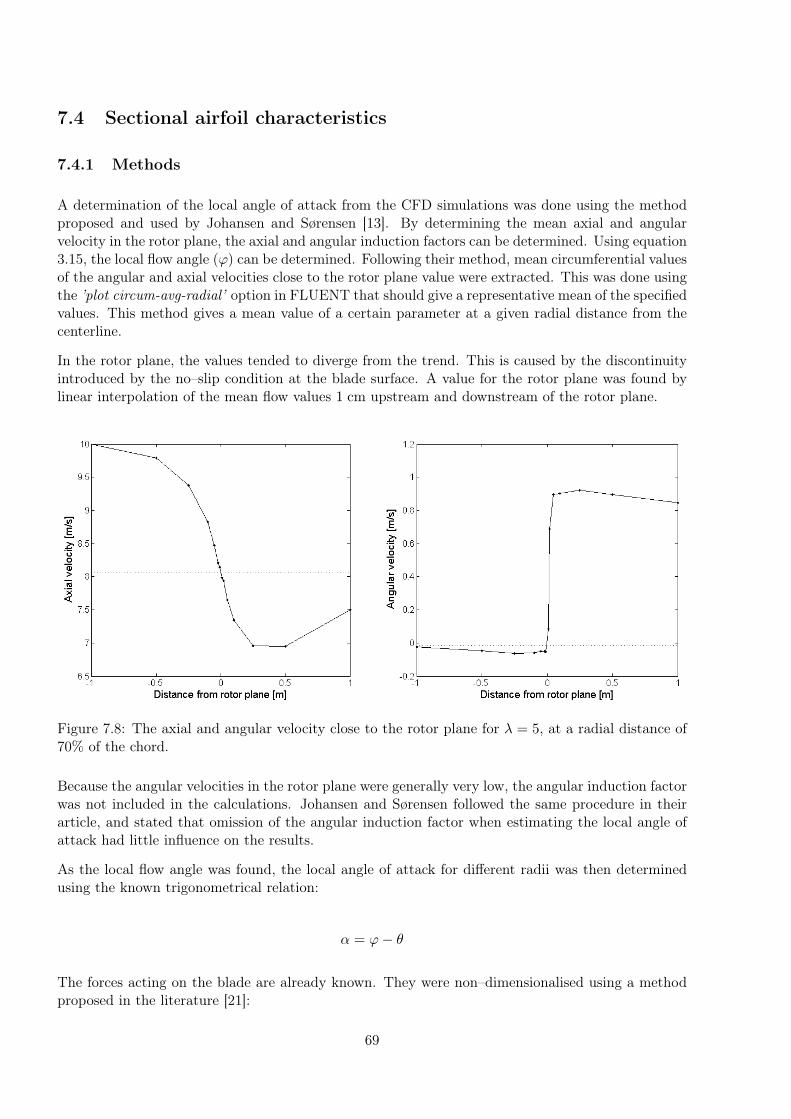
7.4 Sectional airfoil characteristics
7.4.1 Methods
A determination of the local angle of attack from the CFD simulations was done using the methodproposed and used by Johansen and Sørensen [13]. By determining the mean axial and angularvelocity in the rotor plane, the axial and angular induction factors can be determined. Using equation3.15, the local flow angle (ϕ) can be determined. Following their method, mean circumferential valuesof the angular and axial velocities close to the rotor plane value were extracted. This was done usingthe ’plot circum-avg-radial’ option in FLUENT that should give a representative mean of the specifiedvalues. This method gives a mean value of a certain parameter at a given radial distance from thecenterline.
In the rotor plane, the values tended to diverge from the trend. This is caused by the discontinuityintroduced by the no–slip condition at the blade surface. A value for the rotor plane was found bylinear interpolation of the mean flow values 1 cm upstream and downstream of the rotor plane.
Figure 7.8: The axial and angular velocity close to the rotor plane for λ = 5, at a radial distance of70% of the chord.
Because the angular velocities in the rotor plane were generally very low, the angular induction factorwas not included in the calculations. Johansen and Sørensen followed the same procedure in theirarticle, and stated that omission of the angular induction factor when estimating the local angle ofattack had little influence on the results.
As the local flow angle was found, the local angle of attack for different radii was then determinedusing the known trigonometrical relation:
α = ϕ− θ
The forces acting on the blade are already known. They were non–dimensionalised using a methodproposed in the literature [21]:
69

Cn =dFx
12ρC(U2
∞ + (ωr)2)
Ct =dFz
12ρC(U2
∞ + (ωr)2)
When the axial and tangential force coefficients were transformed into local lift and drag coefficients,using the following equations:
Cl = Cn cosϕ− Ct sinϕ (7.5)
Cd = Cn sinϕ+ Ct cosϕ (7.6)
7.4.2 Sectional lift and drag
Figure 7.9 shows the sectional lift and drag coefficients for the wind turbine, plotted against theangle of attack. The figure also includes a lift and drag curve from XFOIL at a Reynolds numberof 1.0 · 105 and a transition criteria of Ncrit = 3.0 for comparison. It is clear that there is a goodcorrespondence between the XFOIL results and the CFD results.
The innermost and outermost sections are found to have a smaller lift slope than what is expectedin the two dimensional case. This is an indication that both tip and root vortices are present. Theinduced downwash from the vortex will reduce the effective angle of attack, resulting in a lower slopeon the Cl curve [4]. It is also clear that rotational augmentation or stall delay is present. The liftcoefficient at r/R = 0.25 is increased far beyond what is expected for an airfoil of infinite span, forangles of attack far into the stalled region.
Figure 7.9: Calculation of local lift and drag coefficients for different tip speed ratios.
Moving toward the tip of the blade, it is clear that tip loss effects do affect the performance of thenear–tip sections. This is seen as a reduction in maximum lift. The r/R = 0.80 section only seemsto be influenced by the tip effects at λ = 3, as it follows the two dimensional results quite well for
70

all other tip speed ratios. The lift coefficients of the r/R = 0.5 and r/R = 0.65 sections do followthe two dimensional results remarkably well. This indicates that the reason for failure in the BEMmodel is related to tip and root effects – effects that the Prandtl tip loss factor seems incapable ofdescribing correctly.
Looking at the drag curve, the correspondence is still good. However, there are indications that stall isprecipitated (or hastened) at low tip speed ratios. At high angles of attack, the drag coefficient seemsto be increased far beyond what is expected in a two dimensional case. As it is only the innermostsection that experiences a stall delay, this might actually be a poor phrase for the observed effect.Rotational augmentation might be a better choice, as the lifting force is augmented, while stall seemsto be precipitated for several radii.
71
7.5 Three dimensional effects
There are several indications that three dimensional effects are present. It is expected that theseeffects are related to separation on the wind turbine blades. In order to investigate where and whenthe flow around the wind turbine blades is separating, a study of cross sectional pressure distributionswas made. The pressure was obtained using the method described in chapter 7.3.2.
The pressure was non–dimensionalised using the method proposed by Sørensen el. al [21]:
−Cp =p∞ − p
12ρC (U2
∞ + (ωr)2)(7.7)
The pressure distribution was studied with the boundary layer theory in mind. Generally, a chordwisepressure gradient on an airfoil is an indication that the boundary layer is attached. Alternatively,pressure distribution with no gradient in the chordwise direction indicates boundary layer separation.In this way the separation point can be determined by looking at the Cp–curve. If there is a gradientupstream of the separated area, it is a sign of boundary layer separation. A gradient downstream ofthe separated area is an indication of boundary layer attachment.
As indicated in the study of spanwise forces, there are indications of massive separation on the bladefor the λ = 3 case. This is evident when looking at figure 7.13, where there are clear indications ofseparation from the middle of the blade and outwards. At r/R = 0.50 the blade seems to be fullystalled, with separation from the leading to the trailing edge of the blade. Closer to the tip, the flowseems to remain attached close to the leading edge.
For r/R = 0.25 it is hard to interpret the Cp curve. There are indications of separation on thesuction side, close to the leading edge. However, the pressure distribution indicates a shear layerreattachment. A closer look at the velocity field at r/R = 0.25 revealed large spanwise velocitycomponents. The flow actually separates at the leading edge, but there is a rapid spanwise flowbelow the separated flow. Because of the high velocity of this flow, the pressure coefficient remainslow over the blade, indicating that separation has not occurred. These radial velocity componentsremain quite large for all spanwise sections, as seen in figure 7.10.
Looking at figure 7.12, it is seen that the spanwise flow occurring at λ = 3 starts at the root of theblade and extends all the way towards the tip. These spanwise velocity components are visible forall tip speed ratios. However, they seem to become more dominant as the blade enters the stalledarea. When the angle of attack is reduced, suction side pressure is reduced. This can be seen fromfigure 7.13. This low pressure area seems to draw air from the root of the blade, pulling it in thespanwise direction.
As the angle of attack is increased, the spanwise flow will grow, eventually ’forcing’ a separation atthe leading edge. But, as the spanwise flow has a rather high velocity, a high lift coefficient can bemaintained for low radial sections.
It is important to notice that earlier studies of this rotational augmentation effect have shown thatthe effect is dependent of rotation. This indicate that centripetal and/or Coriolis forces are importantin the description of the physics behind it. However, it seems like it is the pressure potential thatgets the spanwise flow started.
As the tip speed ratio is increased to λ = 4, the massive leading edge separation disappears. Herethe pressure distributions seem quite normal for all spanwise sections. This is in accordance with
72

Figure 7.10: Vector plot of the fluid velocity relative to the blade at different spanwise sections forλ = 3. The separation is found to occur at the leading edge for all spanwise sections, with a spanwiseflow below the separated air.
the BEM predictions, that gave angles of attack below 12◦ for all spanwise sections (see figure 7.1).However, looking at the CFD results, the predicted angle of attack is close to 15◦ at r/R = 0.25,which means that the blade should be stalled at this point.
Looking closer at figure 7.12, it is clear that there are still quite large spanwise velocity componentsclose to the root of the blade. The effect observed for λ = 3 is observed for λ = 4 as well. There aresigns of leading edge separation close to the root of the blade, but the spanwise velocity componentsmaintains a low pressure on the suction side. Therefore the separation is not visible in the Cp curves.
For λ = 6 the leading edge separation has disappeared, but the three dimensional effects close to theroot are still significant. There are indications of a small recirculation area where the blade meetsthe junction, seen as an increase in spanwise viscous shear (figure 7.11). However, the local angle ofattack near the root of the blade is far below the stall angle for this case.
The fact that separation occurs for low angles of attack indicates that the spanwise componentsobserved for low tip speed ratios do not only depend on the local angle of attack, but also on theblade junction geometry. If the spanwise velocity components depend on the shape of the root of theblade, it would probably be favorable to reduce the size of the gap between the blade and the hub.
73

Figure 7.11: Spanwise viscous shear on the suction side of the blade for a) λ = 3 and b) λ = 6.
This could reduce both the blade root vortex and the spanwise velocity components. The spanwisevelocity components might have a positive effect on the sectional lift coefficients, but they could alsolead to strong dynamic effects.
The reduction of the angle of attack is first seen by a reduction of the suction peak near the leadingedge. The resulting pressure distributions for moderate tip speed ratios have no signs of deviationfrom the expected results.
As the tip speed ratio increases towards 9 and 11, the three dimensional effects tend to disappear. Theangle of attack is reduced and the pressure difference between the suction and pressure side decreases.When the pressure difference is reduced, the potential causing the spanwise flow disappears. Thereduction in pressure difference can be seen from the pressure distributions. For λ = 9 and 11, theflow close to the root section is almost two–dimensional. Even the root vortex seen for the lower tipspeed ratios tend to disappear, as the lift coefficient approaches zero for the root section.
74

Figure 7.12: Particle tracks and spanwise viscous shear stress on the blade suction side for a) λ = 3,b) λ = 4, c) λ = 6, d) λ = 9 and e ) λ = 11.
75

Figure 7.13: Pressure distributions for the λ = 3 (left) and λ = 4 (right) case at five spanwisepositions.
76

Figure 7.14: Pressure distributions for the λ = 5 (left) and λ = 6 (right) case at five spanwisepositions.
77

Figure 7.15: Pressure distributions for the λ = 9 (left) and λ = 11 (right) case at five spanwisepositions.
78

Chapter 8
Conclusions
8.1 Concluding remarks
An experiment conducted in the wind tunnel at NTNU confirmed that the model wind turbine wasworking according to estimates made using a BEM method. However, as the profile used throughoutthe blade has been designed for a Reynolds number twenty times higher than what is expected inthe wind tunnel, the airfoil is exposed to laminar separation. This has been observed in laboratorywork performed by Muyiwa Adaramola [1].
At tip speed ratios below design conditions, severe dynamic effects were observed, probably relatedto stalling of the blade. The BEM method was able to predict the onset of stall, but as a one–dimensional method, the dynamics behind it was not captured.
Initial two–dimensional CFD simulations of the flow around the NREL s826 airfoil were performed inorder to determine reasonable grid parameters for the three–dimensional grid. It was revealed that astructured boundary layer grid with at least 15 cells, and a height of 0.1C was sufficient to capturethe boundary layer flow. When using an unstructured grid in the rest of the domain, the externalgrid growth rate should be kept as low as possible. The use of enhanced wall treatment and the k–ωSST–model gave good predictions of the airfoil forces.
Based on the experience from the initial simulations, a three–dimensional grid was created, and full3D CFD simulations of the wind turbine were conducted. Rotational periodicity was assumed inorder to reduce the size of the grid.
In general, good accordance was observed between the CFD simulations and experimental data. Forlow tip speed ratios the power curve predictions were well within the measured standard deviations,with errors less than 5%. For higher tip speed ratios the errors were somewhat higher. This isexpected to be caused by low grid refinement close to the root of the blade. The thrust was somewhatunderpredicted, which was expected due to the exclusion of wind turbine tower and transmission beltin the CFD model.
Prandtls tip loss factor has been included in the BEM calculations. It is clear that the correctionfactor manages to describe the tip loss effects fairly well for moderate tip speed ratios. Close to thedesign point, the accordance between the BEM and CFD results for tangential forces on the bladeare almost perfectly matched. However, for high tip speed ratios, the BEM method overpredicts thethrust forces near the tip of the blade.
79
The BEM calculations tended to give lower estimates of the thrust force than the CFD model forall operational conditions. But it is clear that the introduction of Glauerts correction factor for highvalues of a improves the results. The power curve is fairly well described for all tip speed ratios, butthe errors tend to be smaller near the design tip speed ratio. Under these operational conditionsthree–dimensional effects are small, and the angle of attack is rather constant over the blade.
A further examination of the forces acting on the blade revealed that there were substantial three–dimensional effects present for low tip speed ratios. These effects caused large spanwise variationsin the force distribution on the blade, combined with evidence of rotational augmentation. Therotational augmentation was visible as sectional lift coefficients near the root of the blade wereincreased far beyond what could be expected for two dimensional flow. However, the rotationalaugmentation was found to occur in cases where there was leading edge separation on the blade.The increased lift was caused by a rapid spanwise flow beneath the separated air. Due to theseobservations, the term ’stall delay’ that is used in the literature is regarded to be a poor phrase, notdescribing the actual physics behind the effect.
There are indications that the three dimensional effects observed near the root of the blade aredependent on the root geometry. Near the root of the blade separation seems to be precipitated dueto a certain leakage of flow around the root edge of the blade. Separation at the root was observedfor a tip speed ratio of 6, where the angle of attack is low and three dimensional effects are expectedto be small. This indicates that an improvement of the root geometry could reduce the spanwise flowon the blade for low tip speed ratios.
8.2 Further work
The BEM method proved to have certain convergence problems in cases where the axial inductionfactor became negative. In these cases the turbine works as a propeller, adding energy to the flow.This occurs close to the root of the blade for high tip speed ratios, and the code needs to be improvedin order to capture these effects.
The Prandtl tip loss factor proved to be unable to predict the spanwise thrust force distributionfor high tip speed ratios. There is a new class of tip loss factor emerging, and several of theseare presented in the literature [20]. It is probable that an improvement of the tip (and hub) losspredictions can improve the BEM predictions.
Future testing of the wind turbine should be conducted at a fixed rotational speed, in order to reducethe change of blade Reynolds number between the different operational conditions. It is importantto keep this speed so high that laminar effects do not become dominant.
The experimental results revealed strong dynamic effects as the blade entered the stalled area. Theseeffects have been discussed in this report, and there are indications that they could be caused bylaminar separation. This could be examined by relatively simple experiments in the wind tunnel.Further studies should be undertaken in order to determine the effects of rotation on transition, andfurthermore if the regular Ncrit transition criteria is applicable for a rotating wind turbine.
The actual physics behind the rotational augmentation found in this study is still incompletelyunderstood and characterised. This calls for further studies on the behavior of rotating wind turbineblades in stalled condition.
80

Bibliography
[1] Muyiwa Adaramola, 2009. Laboratory work in progress.
[2] AIAA. Guide for the verification and validation of computational fluid dynamics simulations,1998. AIAA G-077-1998.
[3] W A Basha and W S Ghaly. Drag Prediction in Transitional Flow over Airfoils. Journal ofAircraft, 44:824 – 832, 2007.
[4] J J Bertin. Aerodynamics for Engineers, 4th ed. Prentice Hall, 1994.
[5] P A Davidson. Turbulence, an introduction for scientists and engineers. Oxford UniversityPress, 2004.
[6] M Drela and H Youngren. XFOIL 6.9 User Primer, 2001.
[7] C Kjaer et. al. Wind Energy - The Facts, 2009.
[8] Fluent. www.fluent.com, 2008. 03.03.2009.
[9] Per Åge Krogstad, 2009. Private communication.
[10] M O L Hansen. Aerodynamics of Wind Turbines, 2nd ed. Earthscan, 2008.
[11] H Hu and Z Yang. An Experimental Study og the Laminar Flow Separation on a Low-Reynolds-Number Airfoil. Journal of Fluids Engineering, 130, 2008.
[12] J Johansen, H Aa Madsen, M Gaunaa, C Bak, and N N Sørensen. Design of a Wind TurbineRotor for Maximm Aerodynamic Efficiency. Wind Energy, 2008.
[13] J Johansen and N N Sørensen. Aerofoil Characteristics from 3d CFD Rotor Computations.Wind Energy, 7:283 – 294, 2004.
[14] V P Jones and B E Launder. The prediction of Laminarization with a Two-Equation Model ofTurbulence. International Journal of Heat and Mass Transfer, 15:301 – 314, 1972.
[15] P B S Lissaman. Low Reynolds Number Airfoil. Ann. Rev. Fluid Mechanics, 15:223 – 239, 1983.
[16] F R Menter. Two-Equation Eddy-Viscosity Turbulence Models for Engineering Applications.AIAA, 32:1598 – 1605, 1994.
[17] C L Rumsey. Apparent Transition Behaviour of widely-used Turbulence Models. InternationalJournal of Heat and Fluid Flow, 28:1460 – 1471, 2007.
[18] H Schlichting and K Gersten. Boundary Layer Teory, 8th ed. Springer, 1999.
81
[19] S J Schreck, N N Sørensen, and M C Robinson. Aerodynamic Structures and Processes inRotationally Augmented Flow Fields. Wind Energy, 10:159 – 178, 2007.
[20] W Z Shen, R Mikkelsen, J N Sørensen, and C Bak. Tip Loss Corrections for Wind TurbineComputations. Wind Energy, 8:457 – 475, 2005.
[21] N N Sørensen, J A Michelsen, and S Schreck. Navier Stokes predictions of the NREL Phase VIrotor in the NASA Ames 80-by-120 Wind Tunnel. AIAA Paper 2002-0031, 2002.
[22] E Sæta. The Blade Element Momentum Method. Project–thesis, 2008.
[23] Nobou Tanaka. World Energy Outlook 2008. IEA, 2008.
[24] H. Tennekes and J. L. Lumley. A First Course in Turbulence, 3rd ed. MIT Press, 1972.
[25] L W Traub and E Cooper. Experimental Investigation of Pressure Measurements and AirfoilCharacteristics at Low Reynolds Numbers. Journal of Aircraft, 45:1322 – 1333, 2008.
[26] H K Versteeg and W Malalasekera. Computational Fluid Dynamics, The finite volume method.Pearson, 2007.
[27] Frank M. White. Viscous Fluid Flow, 3rd ed. McGraw–Hill, Inc, 1991.
[28] David C. Wilcox. Turbulence Modeling for CFD. DCV Industries, Inc, 1994.
[29] J Windte, U Scholz, and R Radespiel. Validierung der RANS-Simulation Laminarer Ablöseblasenauf Profilen. Aerospace and technology, 10:484 – 494, 2006.
[30] Victor Yakhot and Steven A Orszag. Renormalization Group Analysis of Turbulence. I. Basictheory. Journal of Scientific Computing, 1:3 – 51, 1986.
[31] Victor Yakhot and Leslie M Smith. The Renormalization Group, ε-expansion and the Derivationof Turbulence Models. Journal of Scientific Computing, 7:35 – 61, 1992.
82

Appendix A
Appendix
A.1 Calibration curves
A.1.1 Thrust gauge
The calibration curve for the thrust force given i kg was given by:
T = 3.5763Vt,measured − Vt,offset
Vt,gain− 0.0118 (A.1)
The offset voltage was −8.110 V, and the amplifier gain was set to 8. The calibration was done usingweights directly attached to the gauge. The weight box had a mass of 449 g, and masses up to 6 kgwas attached.
Weight [kg ] Volts V − Vt,offset0 -8.110 0
0.449 -7.054 0.1320.949 -5.984 0.265751.449 -4.862 0.4061.949 -3.732 0.547252.449 -2.609 0.6876252.949 -1.366 0.8433.449 -0.379 0.9663753.949 0.740 1.106254.449 1.853 1.2453754.949 2.973 1.3853755.449 4.089 1.5248755.949 5.238 1.66856.449 6.33 1.805
Table A.1: Calibration data for thrust gauge.
83
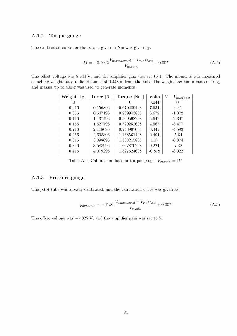
A.1.2 Torque gauge
The calibration curve for the torque given in Nm was given by:
M = −0.2042Vm,measured − Vm,offset
Vm,gain+ 0.007 (A.2)
The offset voltage was 8.044 V, and the amplifier gain was set to 1. The moments was measuredattaching weights at a radial distance of 0.448 m from the hub. The weight box had a mass of 16 g,and masses up to 400 g was used to generate moments.
Weight [kg ] Force [N ] Torque [Nm ] Volts V − Vm,offset0 0 0 8.044 0
0.016 0.156896 0.070289408 7.634 -0.410.066 0.647196 0.289943808 6.672 -1.3720.116 1.137496 0.509598208 5.647 -2.3970.166 1.627796 0.729252608 4.567 -3.4770.216 2.118096 0.948907008 3.445 -4.5990.266 2.608396 1.168561408 2.404 -5.640.316 3.098696 1.388215808 1.17 -6.8740.366 3.588996 1.607870208 0.224 -7.820.416 4.079296 1.827524608 -0.878 -8.922
Table A.2: Calibration data for torque gauge. Vm,gain = 1V
A.1.3 Pressure gauge
The pitot tube was already calibrated, and the calibration curve was given as:
pdynamic = −61.89Vp,measured − Vp,offset
Vp,gain+ 0.007 (A.3)
The offset voltage was −7.825 V, and the amplifier gain was set to 5.
84
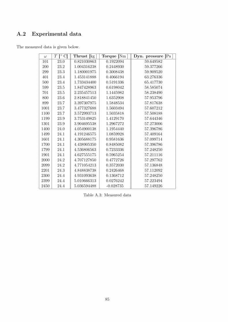
A.2 Experimental data
The measured data is given below.
ω T [◦ C] Thrust [kg ] Torque [Nm ] Dyn. pressure [Pa ]101 23.0 0.821030863 0.1922094 59.649582200 23.2 1.004316238 0.2448930 59.377266299 23.3 1.180001975 0.3008438 59.909520401 23.4 1.453141888 0.4066194 63.276336500 23.4 1.733434400 0.5191336 65.417730599 23.5 1.847428963 0.6198042 58.585074701 23.5 2.235457513 1.1445982 58.238490800 23.6 2.818841450 1.6352908 57.953796899 23.7 3.397307975 1.5848534 57.8176381001 23.7 3.477327688 1.5603494 57.6072121100 23.7 3.572993713 1.5035818 57.5081881199 23.9 3.753149825 1.4129170 57.6443461301 23.9 3.904695538 1.2967272 57.2730061400 24.0 4.054900138 1.1954440 57.3967861499 24.1 4.191246575 1.0859928 57.4091641601 24.1 4.305688175 0.9581636 57.0997141700 24.1 4.438905350 0.8485082 57.3967861799 24.1 4.536806563 0.7233336 57.2482501901 24.1 4.627555175 0.5965254 57.2111162000 24.2 4.707127850 0.4772726 57.2977622099 24.2 4.771054213 0.3572030 57.1368482201 24.3 4.848838738 0.2426468 57.1120922300 24.4 4.931093638 0.1368712 57.2482502399 24.4 5.010666313 0.0276242 57.2234942450 24.4 5.036594488 -0.028735 57.149226
Table A.3: Measured data
85

A.3 Blade design
The blade design used in the BEM–calculations was similar to the original design proposed by Sata[22], however, some changes was made close to the root of the blade. This was done to represent theshape of the actual blade better. The junction part of the blade is represented by keeping the twistangle more or less constant, while reducing the chord length.
r c/R θ
7.5000000e-003 3.0000000e-002 1.2000000e+0022.2500000e-002 3.0000000e-002 1.2000000e+0024.9000000e-002 3.0000000e-002 1.2000000e+0025.5000000e-002 1.1000000e-001 3.8000000e+0016.7500000e-002 1.8096180e-001 3.7054990e+0018.2500000e-002 1.7802475e-001 3.2544100e+0019.7500000e-002 1.7113681e-001 2.8676740e+0011.1250000e-001 1.6250122e-001 2.5261900e+0011.2750000e-001 1.5335073e-001 2.2430330e+0011.4250000e-001 1.4433777e-001 1.9987820e+0011.5750000e-001 1.3578290e-001 1.8034450e+0011.7250000e-001 1.2782281e-001 1.6348850e+0011.8750000e-001 1.2049533e-001 1.4663250e+0012.0250000e-001 1.1378725e-001 1.3067150e+0012.1750000e-001 1.0766085e-001 1.1829070e+0012.3250000e-001 1.0206832e-001 1.0752650e+0012.4750000e-001 9.6959534e-002 8.8827240e+0002.7750000e-001 8.8002408e-002 7.9877430e+0002.9250000e-001 8.4068035e-002 7.2526930e+0003.0750000e-001 8.0446168e-002 6.5649770e+0003.2250000e-001 7.7104257e-002 5.9186800e+0003.3750000e-001 7.1148557e-002 4.7185370e+0003.6750000e-001 6.8486964e-002 4.1316170e+0003.8250000e-001 6.6008976e-002 3.5438940e+0003.9750000e-001 6.3697134e-002 2.9433360e+0004.1250000e-001 6.1535992e-002 2.2185090e+0004.2750000e-001 5.9511861e-002 1.0970280e-0014.4250000e-001 5.7612581e-002 -7.167448e-001
Table A.4: Blade design input to BEM–calculations.
86

A.4 Examination of laminar separation bubbles
Figure A.1: XFOIL calculation at α = 7◦ and Re = 7.5 · 104 with Ncrit = 9.0. The laminarseparation bubble on the suction side is clearly seen from the Cp curve, reattaching at c/C ≈ 0.65.
Figure A.2: XFOIL calculation at α = 14◦ and Re = 7.5 · 104 with Ncrit = 3.0. The transition occurnear the suction peak at the leading edge and no laminar separation is visible. The boundary layerseparates at c/C ≈ 0.45
87
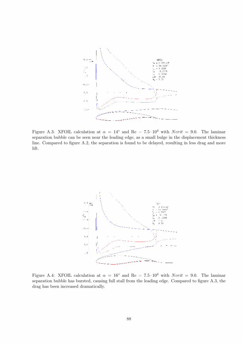
Figure A.3: XFOIL calculation at α = 14◦ and Re = 7.5 · 104 with Ncrit = 9.0. The laminarseparation bubble can be seen near the leading edge, as a small bulge in the displacement thicknessline. Compared to figure A.2, the separation is found to be delayed, resulting in less drag and morelift.
Figure A.4: XFOIL calculation at α = 16◦ and Re = 7.5 · 104 with Ncrit = 9.0. The laminarseparation bubble has bursted, causing full stall from the leading edge. Compared to figure A.3, thedrag has been increased dramatically.
88

A.5 Grid parameters (reduced size)
Grid O X O XI O XIV O XIVa O XIVb O XX# cells 6557 7764 7436 6342 5760 8725External growth rate 1.2 1.2 1.2 1.3 1.45 1.2Nodes in BL 15 20 20 20 20 20BL growth rate 1.24 1.15 1.21 1.21 1.21 1.24BL height 0.05c 0.05c 0.1c 0.1c 0.1c 0.15c
Table A.5: Grid parameters for some of the grids used in the second part of the grid sensitivity study.
A.6 Periodic boundary grid
A figure of the periodic boundary grid is attached.
Figure A.5: Periodic boundary surface grid
89
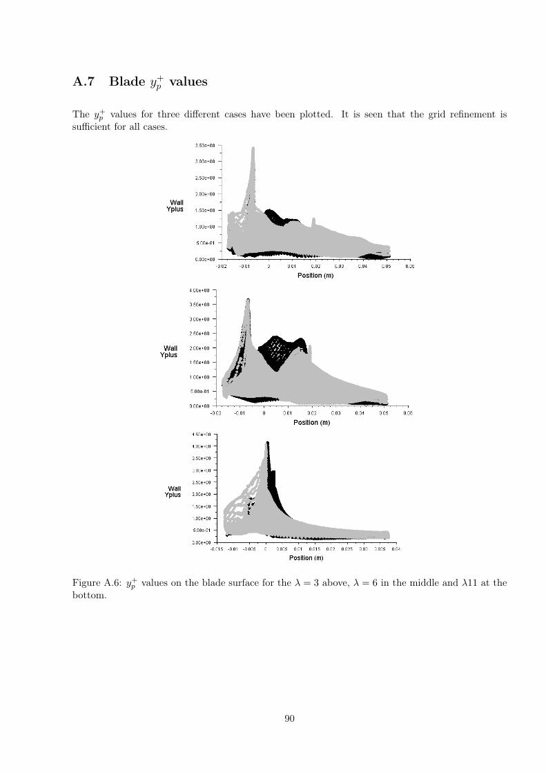
A.7 Blade y+p values
The y+p values for three different cases have been plotted. It is seen that the grid refinement is
sufficient for all cases.
Figure A.6: y+p values on the blade surface for the λ = 3 above, λ = 6 in the middle and λ11 at the
bottom.
90

A.8 Convergence monitoring
A typical convergence history. The solution was started at 4000 iterations, from the λ = 4 case.A non–oscillating solution was found after 1000 iterations, using 1. order discretisation. Then theQUICK scheme was applied, reaching maximum convergence after 1000 iterations more. An addi-tional 500 iterations was taken in order to reduce residuals more, and minimize iterative convergenceerror. Additional iterations was made to reduce the residuals for k, without altering the Cm and Cdresults.
Figure A.7: Convergence history for the λ = 5 case.
91

A.9 Critical Reynolds number for a cylinder
Figure A.8: Cd as a function of Reynolds number for different bodies. From White [27].
92