To appear in The European Journal of Operational Research

Performance Bounds for the Effectiveness of Pooling inMulti-Processing Systems

Saifallah Benjaafar†

Department of Mechanical and Industrial Engineering, University of Minnesota,Minneapolis, Minnesota 55455, USA

Abstract: The need for quantifying the effect of resource pooling on performance of

multi-processing systems arises frequently in the design of a variety of manufacturing,

communication, and service systems. In this paper, we examine the effect of resource

pooling and assess its impact on system performance. In particular, we provide

performance bounds on the effectiveness of several pooling scenarios and discuss

capacity and utilization tradeoffs between independent and pooled systems. We also

propose a methodology for making optimal pooling decisions and describe the

characteristics of this optimal solution. Limitations to the effectiveness of pooling are

identified and conditions under which pooling may degrade performance are discussed.

Key words: Queuing systems; performance evaluation; pooling; optimization

† The author's research was in part supported by the National Science Foundation under grant No. DDM-9309631.

-2-

1. Introduction

Consider a multi-processing system consisting of m facilities. Each facility i has

ni servers and witnesses the arrival of customers at a mean arrival rate λ i. Customers

arriving at facility i require processing with a mean processing time 1/µi. We are

interested in studying the effect that partial or total pooling of these facilities might have

on overall system performance. This problem arises quite frequently in the design of a

variety of manufacturing [Dallery and Stecke 1990] [Calabrese 1992] [Benjaafar 1992]

[Whitt 1992], communication [Smith and Whitt 1981] [Whitt 1992], and computer

systems [Kleinrock 1976] [Malone and Smith 1984].

While it is generally accepted that pooled facilities are more effective than

independent ones [Cooper 1972] [Wolff 1980], this acceptance is often based on

numerical data rather than rigorous mathematical proof. For example, Smith and Whitt

[Smith and Whitt 1981] were the first to formally show that operating a single facility

with n1 + n2 servers was at least as effective as operating two independent facilities with

n1 and n2 servers respectively. They found this to hold for systems where the customer

inter-arrival and service times are identically distributed for all facilities. Recently,

Calabarese [Calabrese 1992] showed that when the average load per server is held

constant in a M/M/m queuing system, average delay strictly decreases with increases in

m. That is, pooling facilities that can be modeled as exponential multi-server queuing

systems always reduces average delay. Dallery and Stecke [Dallery and Stecke 1990],

Stecke and Solberg [Stecke and Solberg 1985], and Buzacott and Shanthikumar

[Buzacott and Shanthikumar 1993] discussed the issue of resource pooling in the context

of closed queuing network models of Flexible Manufacturing Systems (FMS) and found

that system throughput increases with increased pooling.

In this paper, we extend the results of Smith and Whitt [Smith and Whitt 1981]

and Calabrese [Calabrese 1992] by further characterizing the effect of pooling on

performance of open queuing systems. We provide performance bounds on the

-3-

effectiveness of several pooling scenarios and discuss capacity and utilization tradeoffs

between independent and pooled systems. We also propose a methodology for making

optimal pooling decisions and describe the characteristics of this optimal solution.

Finally, we discuss limitations to the effectiveness of pooling and identify conditions

under which pooling may degrade performance.

2. Performance Evaluation

Consider a queuing system consisting of m facilities. Each facility i has ni

servers. Customer arrivals to all facilities are poisson with mean arrival rate λ i = niλ to

facility i and λ > 0. The service times of all servers are exponentially distributed with

mean service rate µ and µ > λ . All facilities are subject to the same average utilization ρ

= λ/µ with 0 < ρ < 1. We use the notation D(n1, n2, …, nm, ρ) to refer to average delay

(before begining service) in a system of m independent facilities with ni servers per

facility, and D(n1 + n2 + … + nm, ρ) to describe average delay for a single facility with

n1 + n2 + … + nm servers. Similarly, we use the notations L(•, ρ), Lq(•, ρ) and W(•, ρ) to

refer respectively to the average number of customers in the system, the average number

of customers in the queue, and the average sojourn time in the system.

Theorem 1: D(n1 + n2 + … + nm, ρ) < D(n1, n2, …, nm, ρ)/m for all positive integer

values of ni , m > 1, and 0 < ρ < 1.

Proof: The average delay in the single facility queuing system is given by

D(n1 + n2 + … + nm, ρ) = C(n1 + n2 + … + nm, ρ)

(n1 + n2 + … + nm)(µ - λ),

where

C(n1 + n2 + … + nm, ρ) = [N!(1 - ρ)

j!(Nρ)N - j∑j = 0

N - 1 + 1]

-1

and is the well known Erlang delay formula (N = n1 + n2 + … + nm). Using the fact that

the delay formula is a strictly decreasing function of N [Calabrese 1992], we have

C(n1 + n2 + … + nm, ρ) < C(ni, ρ),

-4-

for i = 1, 2, …, m, or equivalently

D(n1 + n2 + … + nm, ρ) < C(ni, ρ)

(n1 + n2 + … + nm)(µ - λ).

Multiplying both the numerator and denominator by ni, we get

D(n1 + n2 + … + nm, ρ) < niC(ni, ρ)

(n1 + n2 + … + nm)ni(µ - λ) = ni

(n1 + n2 + … + nm) D(ni, ρ).

Summing for all i = 1, 2, …, m and dividing by m we obtain

D(n1 + n2 + … + nm, ρ) < 1m

ni(n1 + n2 + … + nm)∑

i = 1

m D(ni, ρ).

The theorem follows from the identity

D(n1, n2, …, nm, ρ) = ni(n1 + n2 + … + nm)∑

i = 1

m D(ni, ρ). ◊

Corollary 1: D(mn, ρ) < D(n, ρ)/m and D(m, ρ) < D(1, ρ)/m for all positive integer

values of n, m > 1 and 0 < ρ < 1.

Theorem 1 and corollary 1 state that pooling m facilities, regardless of the number

of servers associated with each facility, results in at least a reduction by a factor of m in

average delay. In addition, corollary 1 shows that the average delay in a facility with m

servers is smaller than the average delay in a single server facility by at least a factor of

m.

Corollary 2: Lq(n1 + n2 + … + nm, ρ) < 1m Lq(ni, ρ)∑

i = 1

m for all positive integer values of

ni , m > 1 and 0 < ρ < 1.

Proof: Using the fact that

D(n1 + n2 + … + nm, ρ) < C(ni, ρ)

(n1 + n2 + … + nm)(µ - λ)

and multiplying both sides by (n1 + n2 … + nm)λ , we get by virtue of Little's Law:

Lq(n1 + n2 … + nm) < Lq(ni, ρ).

Summing over i = 1, 2, … m leads to:

-5-

Lq(n1 + n2 + … + nm, ρ) < 1m Lq(ni, ρ)∑

i = 1

m. ◊

Corollary 3: Lq(mn, ρ) < Lq(n, ρ) and Lq(m, ρ) < Lq(1, ρ) for all positive integer values

of ni , m > 1 and 0 < ρ < 1.

Proposition 1: D(m, ρ) < (m - r)D(m - r, ρ)/m for all positive integer values of m and

r (r < m) and for 0 < ρ < 1.

Proof: The proof follows from noting that

D(m, ρ) < C(m - r, ρ)

m(µ - λ) =

(m - r)C(m - r, ρ)

m(m - r)(µ - λ) =

(m - r)D(m - r, ρ)m . ◊

A special instance of proposition 1 is when r = 1 for which we have

D(m, ρ) < (m - 1)D(m - 1, ρ)/m.

This gives us a bound on the reduction in average delay due to a unit increase in the

number of pooled servers. This result can also be used to show that D(m, ρ) is a strictly

decreasing function of m for fixed ρ.

It is interesting to note that the reduction factor (m - 1)/m in the above inequality

is an increasing and concave function of m with a limit of 1. This leads us to conjecture

that the marginal reduction in average delay decreases with increases in m. In other

words, D(m, ρ) is a convex function of m. This fact is supported by numerical data as

shown in Figure 1. In fact, numerical data support an even stronger result, that of the

convexity of the delay probability C(m, ρ) as illustrated in Figure 2.

Conjecture 1: C(m, ρ) is a strictly decreasing and convex function of m for fixed ρ where

m is a positive integer and 0 < ρ < 1.

The first part of the conjecture (i.e. C(m, ρ) is strictly decreasing in m) has been

shown to hold by Calabrese [Calabrese 1992]. The convexity of C(m, ρ) appears to be

more difficult to prove. Supporting argument can be found by making the independence

assumption regarding the server availability probabilities in a multi-server queue (a very

-6-

0

4

8

12

16

20

0 5 10 15 20 25 30

ρ = 0.8

m

ρ = 0.6

ρ = 0.95

ρ = 0.9

ρ = 0.4

Ave

rage

del

ay

Figure 1 Average delay (D(m, ρ)) versus pooling (µ = 1)

0

0.2

0.4

0.6

0.8

1

0 20 40 60 80 100

ρ = 0.4

m

ρ = 0.6ρ = 0.8

ρ = 0.99

ρ = 0.95

ρ = 0.9

Prob

abili

ty o

f de

lay

Figure 2 Probability of delay, (C(m, ρ)), versus pooling

-7-

crude approximation that is nevertheless extensively used in mean value analysis (MVA)

of queuing networks [Suri and Hildebrant 1984]):

C(m, ρ) ≈ C(1, ρ)∏i = 1

m = ρm .

The above approximation is clearly a strictly decreasing and convex function of m.

Corollary 4: D(m, ρ) is a strictly decreasing and convex function of m for fixed ρ where

m is a positive integer and 0 < ρ < 1.

Proof: The proof follows from the fact that D(m, ρ) is the product of two strictly

decreasing positive and convex functions, C(m, ρ) and 1/m(µ - λ). ◊

The convexity property is important since it means that increased pooling has a

diminishing effect on performance. In fact, as suggested by Figure 1, most of the

reduction in average delay is realized with relatively small increases in m. Thus, in a

multi-facility environment, a partial pooling of these facilities may almost be as effective

as a total one.

Figure 1 also suggests that the steepness in D(m, ρ) is a strictly increasing

function of ρ. That is, the difference

δ(m, ρ) = D(m, ρ) - D(m + 1, ρ)

is increasing in ρ.

Conjecture 2: δ(m, ρ) is a strictly increasing function of ρ where m is a positive integer

and 0 < ρ < 1.

The above conjecture simply states that the expected decrease in average delay

increases with system loading. This means that pooling is relatively more valuable for

heavily loaded systems. .

In addition to its effect on mean performance, pooling is found to have a similar

effect on performance variance.

Theorem 2: Delay variance in a facility consisting of m servers, SD(m, ρ), is a strictly

decreasing function of m for fixed ρ where 0 < ρ < 1 and m is a positive integer.

-8-

Proof: The value of delay variance in an m-server queuing system is given by [Kapadia

and Hsi 1978]

SD(m, ρ) = G(m, ρ)

[mµ(1 - ρ )]2,

where

G(m, ρ) = C(m, ρ)(2 - C(m, ρ)).

The value of the difference G(m, ρ) - G(m + 1, ρ) is given by

G(m, ρ) - G(m + 1, ρ) = 2C(m, ρ) - C(m, ρ)2 - 2C(m + 1, ρ) + C(m + 1, ρ)2

= 2(C(m, ρ) - C(m + 1, ρ)) -

(C(m, ρ) + C(m + 1, ρ))(C(m, ρ) - C(m + 1, ρ)).

Since C(m, ρ) - C(m + 1, ρ) > 0 and C(m, ρ) + C(m + 1, ρ) < 2, we have G(m, ρ) -

G(m + 1, ρ) > 0 which immediately leads to the desired result. ◊

Theorem 2 allows us to obtain bounds on delay variance similar to those obtained

for average delay. For the sake of brevity, we only list the following two results. The

notation SD(n1, n2, …, nm, ρ) and σD(n1, n2, …, nm, ρ) are used to denote the weighted

average delay variance and standard deviation associated with m independent facilities

such that

SD(n1, n2, …, nm, ρ) = ni

2

(n1 + n2 + … + nm)2SD(ni, ρ)∑

i = 1

m

and

σD(n1, n2, …, nm, ρ) = ni

(n1 + n2 + … + nm)σD(ni, ρ)∑

i = 1

m.

Proposition 2: SD(n1 + n2 + … + nm, ρ) < SD(n1, n2, …, nm, ρ)/m for all positive integer

values of ni, m > 1, and 0 < ρ < 1.

Proof: The value of delay variance in the pooled system is given by

SD(n1 + n2 + … + nm, ρ) = G(n1 + n2 + … + nm, ρ)

[(n1 + n2 + … + nm)µ(1 - ρ )]2

-9-

Using the fact that G(•, ρ) is a strictly decreasing function of the number of servers, we

have

SD(n1 + n2 + … + nm, ρ) < G(ni, ρ)

[(n1 + n2 + … + nm)µ(1 - ρ )]2 = ni

2

(n1 + n2 + … + nm)2SD(ni, ρ).

for i = 1, 2, …, m. Summing for all i = 1, 2, …, m and dividing by m, we obtain

SD(n1 + n2 + … + nm, ρ) < 1m

ni2

(n1 + n2 + … + nm)2SD(ni, ρ)∑

i = 1

m,

from which we have the result

SD(n1 + n2 + … + nm, ρ) < SD(n1, n2, …, nm, ρ)/m . ◊

Corollary 5: SD(mn, ρ) < SD(n, ρ)/m2 and SD(m, ρ) < SD(1, ρ)/m2 for all positive

integer values of n, m > 1 and 0 < ρ < 1.

Proof: Similar to that of corollary 1. Note that for standard deviation we have σD(mn, ρ)

< σD(n, ρ)/m and σD(m, ρ) < σD(1, ρ)/m. ◊

Conjectures similar to those made with respect to average delay can be extended

to delay variance. As suggested by Figure 3, delay variance is a convex function of

pooling with the degree of convexity increasing with system loading ρ. Again, this

means that the effect of pooling is of the diminishing kind with much of the variance

reduction occurring at relatively low levels of pooling and larger reductions realized for

highly loaded systems.

-10-

0

20

40

60

80

100

0 1 2 3 4 5 6

m

ρ = 0.4ρ = 0.6

ρ = 0.8

ρ = 0.9

Del

ay v

aria

nce

7 8 9 10

Figure 3 Delay variance versus pooling (µ = 1)

3. The Efficiency of Pooling Systems

In this section we address the following two questions: (1) Given n pooled servers

providing a certain service level γ, what is the equivalent number m(γ, n, ρ) of

independent servers required to maintain the same service level (e.g. average delay) when

both systems are subject to the same overall load? and (2) Given n independent servers

providing a service level γ and subject each to a server utilization ρ, by how much server

utilization can be increased when all m servers are pooled while still maintaining the

same service level. These two questions address important issues regarding the potential

capacity savings and productivity increases due to pooling.

3.1 Pooling versus Capacity

Consider a single facility consisting of n servers. The facility is subject to an

average load nλ so that average utilization per server is ρ =λ/µ. The service level

provided by this facility as measured say by average delay is referred to as γ. We use the

-11-

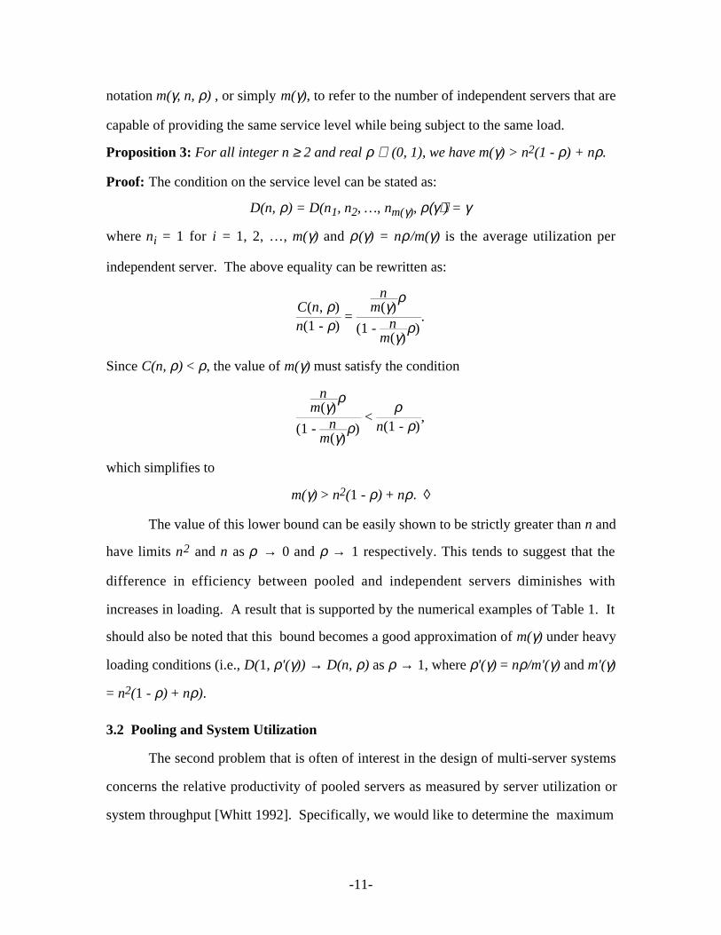
notation m(γ, n, ρ) , or simply m(γ), to refer to the number of independent servers that are

capable of providing the same service level while being subject to the same load.

Proposition 3: For all integer n ≥ 2 and real ρ ∈ (0, 1), we have m(γ) > n2(1 - ρ) + nρ.

Proof: The condition on the service level can be stated as:

D(n, ρ) = D(n1, n2, …, nm(γ), ρ(γ)) = γ

where ni = 1 for i = 1, 2, …, m(γ) and ρ(γ) = nρ/m(γ) is the average utilization per

independent server. The above equality can be rewritten as:

C(n, ρ)n(1 - ρ)

=

nm(γ)

ρ

(1 - nm(γ)

ρ).

Since C(n, ρ) < ρ, the value of m(γ) must satisfy the condition

nm(γ)

ρ

(1 - nm(γ)

ρ) <

ρn(1 - ρ)

,

which simplifies to

m(γ) > n2(1 - ρ) + nρ. ◊

The value of this lower bound can be easily shown to be strictly greater than n and

have limits n2 and n as ρ → 0 and ρ → 1 respectively. This tends to suggest that the

difference in efficiency between pooled and independent servers diminishes with

increases in loading. A result that is supported by the numerical examples of Table 1. It

should also be noted that this bound becomes a good approximation of m(γ) under heavy

loading conditions (i.e., D(1, ρ'(γ)) → D(n, ρ) as ρ → 1, where ρ'(γ) = nρ/m'(γ) and m'(γ)

= n2(1 - ρ) + nρ).

3.2 Pooling and System Utilization

The second problem that is often of interest in the design of multi-server systems

concerns the relative productivity of pooled servers as measured by server utilization or

system throughput [Whitt 1992]. Specifically, we would like to determine the maximum

-12-

Table 1 Pooling versus Capacity(m'(γ) = n2(1 - ρ) + nρ; ρ'(γ) = nρ/m'(γ))

nρ 0.2 0.4 0.5 0.6 0.8 0.9 0.95 0.99

m'(γ) 3.60 3.20 3.00 2.80 2.40 2.20 2.10 2.00

2 D(n, ρ) .04 .19 .33 .56 1.77 4.26 9.25 49.3

D(1, ρ'(γ)) .13 .33 .5 .75 2 4.49 9.5 49.5

m'(γ) 7.8 6.6 6 5.4 4.2 3.6 3.3 3.0

3 D(n, ρ) .01 .07 .16 .30 1.07 2.72 6.04 32.7

D(1, ρ'(γ)) .08 .22 .33 .5 1.33 2.99 6.33 33

m'(γ) 13.6 11.2 10 8.79 6.4 5.2 4.6 4.12

4 D(n, ρ) .003 .04 .09 .18 .75 1.97 4.45 24.44

D(1, ρ'(γ)) .06 .17 .25 .38 1 2.25 4.75 24.75

m'(γ) 21 17 15 13 9 7 6 5.2

5 D(n, ρ) .001 .02 .05 .12 .55 1.52 3.51 19.5

D(1, ρ'(γ)) .05 .13 .2 .3 .8 1.79 3.79 19.8

m'(γ) 82 64 55 46 28 19 14.5 10.9

10 D(n, ρ) 0.000 .001 .007 .025 .20 .67 1.653 9.6

D(1, ρ'(γ)) .02 .07 .1 .15 .4 .9 1.89 9.9

m'(γ) 324 248 210 171 96 58 39 23.79

20 D(n, ρ) 0.00 .00 .00 .00 .06 .27 .27 4.7

D(1, ρ'(γ)) .01 .03 .05 .08 .2 .45 .95 4.9

m'(γ) 1288 976 820 663 351 196 118 55

40 D(n, ρ) 0.00 .00 .00 .00 .019 .17 .13 2.41

D(1, ρ'(γ)) .006 .02 .03 .04 .1 .23 .48 2.47

m'(γ) 2010 1520 1275 1030 540 295 172 74

50 D(n, ρ) 0.000 .000 .000 .000 .008 .07 .25 1.83

D(1, ρ'(γ)) .005 .01 .02 .03 .08 .18 .38 1.98

m'(γ) 8020 6040 5050 4059 2080 1090 595 198

100 D(n, ρ) .000 .000 .000 .000 .001 .02 0.10 0.88

D(1, ρ'(γ)) .003 .007 .01 .015 .04 .09 .19 .99

-13-

amount of additional utilization or throughput that can be achieved when a set of

independent facilities are pooled, while still maintaining the same service level.

We consider a system consisting of n independent servers providing a service

level γ when average utilization per server is ρ. We are interested in characterizing the

factor α(γ) by which server utilization can be increased if the n servers are pooled into a

single facility with the facility still providing the same service level γ.

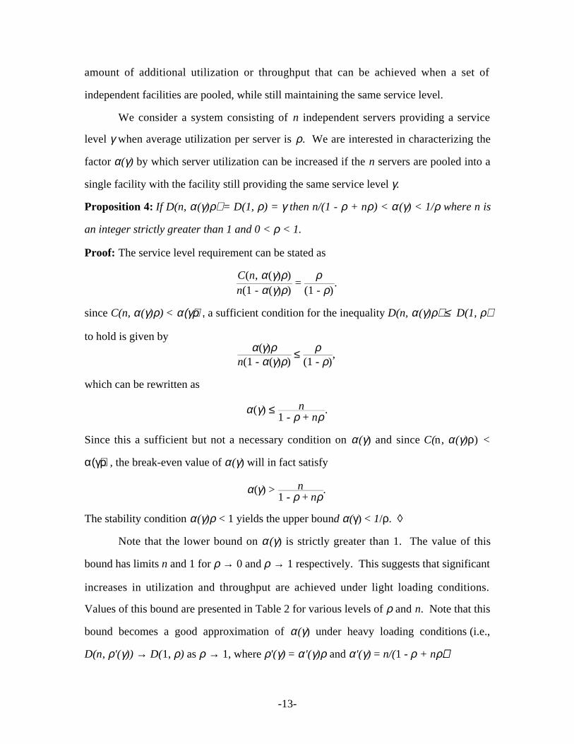
Proposition 4: If D(n, α(γ)ρ) = D(1, ρ) = γ then n/(1 - ρ + nρ) < α (γ) < 1/ρ where n is

an integer strictly greater than 1 and 0 < ρ < 1.

Proof: The service level requirement can be stated as

C(n, α(γ)ρ)n(1 - α(γ)ρ)

= ρ

(1 - ρ).

since C(n, α(γ)ρ) < α(γ)ρ, a sufficient condition for the inequality D(n, α(γ)ρ) ≤ D(1, ρ)

to hold is given byα(γ)ρ

n(1 - α(γ)ρ) ≤

ρ(1 - ρ)

,

which can be rewritten as

α(γ) ≤ n1 - ρ + nρ

.

Since this a sufficient but not a necessary condition on α(γ) and since C(n , α(γ)ρ) <

α(γ)ρ, the break-even value of α(γ) will in fact satisfy

α(γ) > n1 - ρ + nρ

.

The stability condition α(γ)ρ < 1 yields the upper bound α(γ) < 1/ρ. ◊

Note that the lower bound on α (γ) is strictly greater than 1. The value of this

bound has limits n and 1 for ρ → 0 and ρ → 1 respectively. This suggests that significant

increases in utilization and throughput are achieved under light loading conditions.

Values of this bound are presented in Table 2 for various levels of ρ and n. Note that this

bound becomes a good approximation of α(γ) under heavy loading conditions (i.e.,

D(n, ρ'(γ)) → D(1, ρ) as ρ → 1, where ρ'(γ) = α '(γ)ρ and α'(γ) = n/(1 - ρ + nρ)).

-14-

Table 2 Pooling and System Utilization(α '(γ) = n/(1 - ρ + nρ); ρ'(γ) = α '(γ)ρ)

nρ 0.2 0.4 0.5 0.6 0.8 0.9 0.95 0.99

α'(γ) 1.67 1.42 1.33 1.25 1.11 1.05 1.02 1.01

2 D(1, ρ) .25 .67 1.0 1.5 4.0 8.99 18.99 99

D(n, ρ'(γ)) .13 .48 .8 1.28 3.76 8.76 18.75 98.75

α'(γ) 2.14 1.67 1.5 1.37 1.15 1.07 1.03 1.01

3 D(1, ρ) .25 .67 1.0 1.5 4.0 8.99 18.99 99

D(n, ρ'(γ)) .09 .44 .75 1.24 3.72 8.71 18.7 98.7

α'(γ) 2.50 1.82 1.6 1.43 1.17 1.08 1.03 1.01

4 D(1, ρ) .25 .67 1.0 1.5 4.0 8.99 18.99 99

D(n, ρ'(γ)) .086 .432 .745 1.230 3.71 8.70 18.70 98.69

α'(γ) 2.78 1.92 1.67 1.47 1.19 1.09 1.04 1.01

5 D(1, ρ) .25 .67 1.0 1.5 4.0 8.99 18.99 99

D(n, ρ'(γ)) .083 .430 .744 1.229 3.71 8.69 18.70 98.69

α'(γ) 3.57 2.17 1.81 1.56 1.21 1.09 1.04 1.01

10 D(1, ρ) .25 .67 1.0 1.5 4.0 8.99 18.99 99

D(n, ρ'(γ)) .085 .44 .76 1.25 3.74 8.73 18.73 98.73

α'(γ) 4.17 2.32 1.9 1.61 1.23 1.10 1.04 1.01

20 D(1, ρ) .25 .48 1.0 1.5 4.0 8.99 18.99 99

D(n, ρ'(γ)) .101 .48 .80 1.29 3.79 8.78 18.78 98.78

α'(γ) 4.55 2.41 1.95 1.64 1.24 1.10 1.05 1.01

40 D(1, ρ) .25 .67 1.0 1.5 4.0 8.99 18.99 99

D(n, ρ'(γ)) .12 .52 .84 1.34 3.83 8.83 18.83 98.82

α'(γ) 4.63 2.43 1.96 1.64 1.24 1.10 1.05 1.01

50 D(1, ρ) .25 .67 1.0 1.5 4.0 8.99 18.99 99

D(n, ρ'(γ)) .13 .53 .86 1.35 3.85 8.85 18.85 98.86

α'(γ) 4.81 2.46 1.98 1.66 1.25 1.10 1.05 1.01

100 D(1, ρ) .26 .67 1.0 1.5 4.0 8.89 18.99 99

D(n, ρ'(γ)) .16 .57 .89 1.39 3.89 9.01 18.89 98.92

-15-

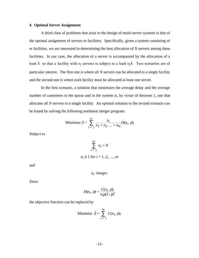
4. Optimal Server Assignment

A third class of problems that arise in the design of multi-server systems is that of

the optimal assignment of servers to facilities. Specifically, given a system consisting of

m facilities, we are interested in determining the best allocation of N servers among these

facilities. In our case, the allocation of a server is accompanied by the allocation of a

load λ so that a facility with ni servers is subject to a load niλ . Two scenarios are of

particular interest. The first one is where all N servers can be allocated to a single facility

and the second one is where each facility must be allocated at least one server.

In the first scenario, a solution that minimizes the average delay and the average

number of customers in the queue and in the system is, by virtue of theorem 1, one that

allocates all N servers to a single facility. An optimal solution to the second scenario can

be found by solving the following nonlinear integer program:

Minimize Z = ni

n1 + n2 … + nmD(ni, ρ)∑

i = 1

m

Subject to

ni∑i = 1

m = N

ni ≥ 1 for i = 1, 2, …, m

and

ni: integer.

Since

D(ni, ρ) = C(ni, ρ)niµ(1- ρ)

,

the objective function can be replaced by

Minimize Z = C(ni, ρ)∑i = 1

m.

-16-

Assuming that conjecture 1 holds (i.e. that C(ni, ρ) is a decreasing and convex

function), an optimal solution can be obtained using marginal analysis as described in

[Fox 1966] (see also appendix). Before characterizing the optimal solution, we prove the

following proposition.

Proposition 5: D(n, n, ρ) ≤ D(n - 1, n + 1, ρ) for any integer n strictly greater than 1

and for 0 < ρ < 1.

Proof: The difference D(n - 1, n + 1, ρ) - D(n, n, ρ) is given by:

D(n - 1, n + 1, ρ) - D(n, n, ρ) = n - 12n

[C(n - 1, ρ)

(n - 1)µ(1 - ρ)] + n + 1

2n[

C(n + 1, ρ)(n + 1)µ(1 - ρ)

] - 2 n2n

[C(n, ρ)

nµ(1 - ρ)]

which simplifies to

D(n - 1, n + 1, ρ) - D(n, n, ρ) = 12nµ(1 - ρ)

[C(n - 1, ρ) + C(n + 1, ρ) - 2C(n, ρ)].

Using the result of conjecture 1 concerning the convexity of C(n, ρ), we have

C(n - 1, ρ) + C(n + 1, ρ) - 2C(n, ρ) ≥ 0.

Consequently the difference D(n - 1, n + 1, ρ) - D(n, n, ρ) is non-negative. ◊

Theorem 3: An optimal allocation vector n* = {n1*, n2*, …, nm*} satisfies the property:

maxi ≠ j(ni* - nj*) ≤ 1

for all ni* and nj* belonging to n*.

Proof: The theorem states that the difference in the number of servers allocated to any

pair of facilities does not exceed 1. The proof can be obtained by noting that in the

iterative procedure of Fox's algorithm (see appendix) no facility will receive two or more

consecutive allocations of servers. For instance let's assume that at stage k facility i

becomes the facility with the largest number of servers, then at stage k + 1, facility i will

certainly not be selected again since a larger marginal decrease in average delay will be

realized from any facility with at least one less server. ◊

Corollary 6: Let N = mn, then the optimal allocation vector is given by:

n* = {n1* = n , n2* = n, …, nm* = n}

for all positive integer values of n and m.

-17-

Theorem 3, proposition 5 and corollary 6 show that a balanced allocation of

servers between facilities is optimal unless total server pooling is allowed. It also shows

that when a perfectly balanced allocation is not possible (i.e. when N is not a multiple of

m), the difference between the numbers of allocated servers to any pair of facilities does

not exceed 1. These results are different from those we would obtain if there were

flexibility in the load allocation. In fact, Calabrese [Calabrese 1992] showed through

numerical examples that optimal configurations are, in that case, unbalanced both in their

server and load allocations. A similar result was observed in the context of central server

closed queuing networks by Dallery and Stecke [Dallery and Stecke 1990] and Stecke

and Solberg [Stecke and Solberg 1984].

5. Pooling and Processing Variety

In this section, we consider limitations to the applicability of the results of

previous sections. In particular, we discuss conditions where pooling may result in

performance degradation. This has been observed to occur in heterogeneous

environments (e.g. environments with non-identical servers and/or multiple class

customers). For instance, Smith and Whitt [Smith and Whitt 1981] provided examples

where pooling server groups with different service time distributions may actually

degrade performance. In this section, we extend this result by characterizing general

conditions under which pooling may be inefficient. Specifically, we consider systems

with multiple customer classes where different classes require different service times.

For the sake of clarity, we restrict our discussion to a system with m customer

classes and m facilities where each facility consists of a single server. Customers of class

i , i = 1, 2, …, m, arrive according to a poisson distribution with mean arrival rate λ i and

require an exponentially distributed processing time with mean 1/µi with µi > λ i. When

the m facilities are operated independently, each facility is dedicated to one customer

class. When the m facilities are pooled into a single one, customers are assigned to the

-18-

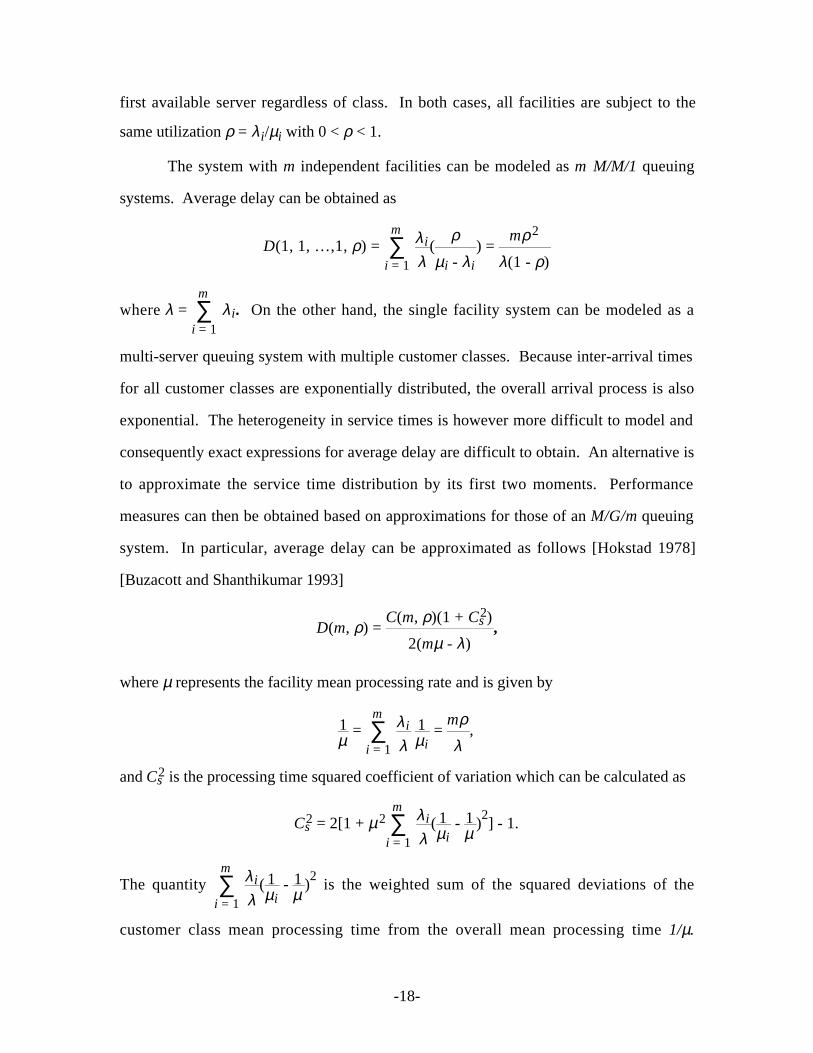
first available server regardless of class. In both cases, all facilities are subject to the

same utilization ρ = λ i/µi with 0 < ρ < 1.

The system with m independent facilities can be modeled as m M/M/1 queuing

systems. Average delay can be obtained as

D(1, 1, …,1, ρ) = λ i

λ(

ρ

µi - λi

) = mρ2

λ(1 - ρ)∑

i = 1

m

where λ = λ i∑i = 1

m. On the other hand, the single facility system can be modeled as a

multi-server queuing system with multiple customer classes. Because inter-arrival times

for all customer classes are exponentially distributed, the overall arrival process is also

exponential. The heterogeneity in service times is however more difficult to model and

consequently exact expressions for average delay are difficult to obtain. An alternative is

to approximate the service time distribution by its first two moments. Performance

measures can then be obtained based on approximations for those of an M/G/m queuing

system. In particular, average delay can be approximated as follows [Hokstad 1978]

[Buzacott and Shanthikumar 1993]

D(m, ρ) = C(m, ρ)(1 + Cs

2)

2(mµ - λ),

where µ represents the facility mean processing rate and is given by

1µ

= λ i

λ 1µi

∑i = 1

m =

mρ

λ,

and Cs2 is the processing time squared coefficient of variation which can be calculated as

Cs2 = 2[1 + µ2 λ i

λ( 1µi

- 1µ

)2] - 1∑

i = 1

m.

The quantity λ i

λ( 1µi

- 1µ

)2∑

i = 1

m is the weighted sum of the squared deviations of the

customer class mean processing time from the overall mean processing time 1/µ.

-19-

Consequently, it can be thought of as the variance of the processing time means.

Similarly, the quantity C1/µ2 = µ2 λ i

λ( 1µi

- 1µ

)2∑

i = 1

m can be used to denote the squared

coefficient of variation in the processing time means. The expression for average delay

can then be rewritten as

D(m, ρ) = C(m, ρ)(1 + C1/µ

2 )

mµ - λ.

As it can be easily verified from the above expression, most of our previous

results regarding the superiority of pooling may not hold any longer. Average delay is

not always a decreasing function of m. In fact, given large enough differences between

the mean processing times of different customer classes, the value of C1/µ2 may increase

with m. The increase in C1/µ2 may then offset any gains resulting from pooling. A bound

on the value of C1/µ2 for which this may occur can be obtained by evaluating the ratio of

average delay in an independent system to that of a pooled one. This ratio is given by

D(1, 1, …, 1, ρ)D(m, ρ)

=

mρ2

λ(1 - ρ)

C(m, ρ)(1 + C1/µ2 )

mµ - λ

= mρ

C(m, ρ)(1 + C1/µ2 )

.

For the independent system to have a smaller average delay, the above ratio needs to be

less than or equal to one, which leads to

C1/µ2 ≥

mρC(m, ρ)

- 1.

The above bound means that pooling will result in a degradation of performance

whenever the variability in the processing requirements of the different customer classes

exceeds the above value. This bound could be used to determine if pooling would be of

any benefit and to identify which customer classes, if any, should be grouped together.

-20-

A lower bound on the above break-even value of C1/µ2 can be obtained by noting

that an upper bound on C(m, ρ) is given by ρ. Substituting ρ for C(m, ρ) leads to

C1/µ2 > m - 1.

It should be noted that this value is generally high. For example, for m = 2, C1/µ2

needs

to be at least greater than 1 (a relatively high coefficient of variation). Thus, if we had

two customer classes, with one of the classes having a unit mean processing time, the

other class needs to have a mean processing time that is more than 7 times larger at ρ =

0.9 in order for the independent system to become more desirable.

These approximations were validated by a series of simulation experiments. A

sample of the simulation results is displayed in Table 3 for an example system of two

servers and two customer classes. Average delay values for both the independent and the

pooled system are obtained for various levels of ρ and C1/µ2 . Values of C1/µ

2 were

obtained by varying the mean processing time, 1/µ2, of one of the customer classes while

keeping that of the other one, 1/µ1, constant at unity.

It can be verified that the values of C1/µ2 for which the independent system has a

smaller average delay are within the above prescribed bounds (see Table 4). In fact, the

bounds become good approximations of the breakeven value of C1/µ2 at high levels of

utilization. Note also that pooled systems become less tolerant of processing variety as

utilization increases. For instance, for ρ = 0.5, the independent system does not result in

lower delays until 1/µ2 exceeds 11. This value is only 6 for ρ = 0.9.

Finally, we must warn that processing variety is not to be confused with

processing variance. The latter typically refers to variability in the processing times of a

given customer class. Contrary to processing variety, increases in processing variance

tend to increase the desirability of pooled systems. This can be seen by considering a

system consisting of m servers and a single customer class with a mean processing time

-21-

Table 3 Average delay for pooled and independent systems

ρ 0.5 0.8 0.9 0.99

µ2-1; C1/µ

2 D(1, 1, ρ) D(2, ρ) D(1, 1, ρ) D(2, ρ) D(1, 1, ρ) D(2, ρ) D(1, 1, ρ) D(2, ρ)

1; 0.00 1.00 0.33 4.00 1.76 9.00 4.31 99.00 57.3

2; 0.12 1.33 0.49 5.33 2.61 12.00 6.32 132.00 78.8

3; 0.33 1.5 0.63 6.00 3.53 13.50 8.59 148.50 90.58

4; 0.56 1.6 0.79 6.40 4.37 14.40 10.65 158.40 106.3

5; 0.80 1.67 0.91 6.67 5.15 15.00 12.04 165.00 109

6; 1.04 1.71 1.09 6.86 5.85 15.43 14.66 169.71 114

7; 1.29 1.75 1.23 7.00 6.96 15.75 16.38 173.25 116

8; 1.53 1.78 1.31 7.11 7.79 16.00 19.16 176.00 131

9; 1.78 1.8 1.46 7.20 8.76 16.20 20.59 178.20 220

10; 2.03 1.81 1.61 7.27 9.71 16.36 23.74 180.00 249

11; 2.27 1.83 1.67 7.33 10.45 16.50 25.37 181.50 252

12; 2.52 1.85 1.85 7.38 11.19 16.62 28.19 182.77 323

13; 2.77 1.86 1.89 7.43 12.36 16.71 29.48 183.86 333

14; 3.02 1.87 2.07 7.47 13.07 16.80 30.50 184.80 360

15; 3.27 1.875 2.15 7.50 13.75 16.87 32.77 185.62 364

16; 3.52 1.882 2.32 7.53 14.75 16.94 34.29 186.35 368

17; 3.76 1.889 2.36 7.56 15.31 17.00 34.94 187.00 371

18; 4.01 1.895 2.53 7.58 15.87 17.05 38.66 187.58 374

19; 4.26 1.900 2.74 7.60 17.17 17.10 39.29 188.10 383

20; 4.51 1.905 2.87 7.62 18.05 17.14 42.63 188.57 391

Table 4 Average delay ratio bounds

ρ 2ρ/C(2, ρ) - 1

0.5 3.00

0.8 2.25

0.9 2.11

0.99

-22-

1/µ and a squared coefficient of variation Cs2. The expression for average delay in a

system of m independent servers, assuming a balanced load allocation among servers, can

then be calculated as

D(1, 1, …, 1, ρ) = ρ(1 + Cs

2)

2(µ - λm ),

while that of m pooled severs can be approximated as

D(m, ρ) = C(m, ρ)(1 + Cs

2)

2m(µ - λm ).

Average delay for the pooled system is evidently always smaller than that of the

independent one. More importantly, the degree of convexity in D(m, ρ) can be easily

shown to strictly increase with increases in Cs2. This means that the difference between

the pooled and independent systems strictly increases with increases in Cs2. In other

words, pooling becomes more desirable with higher processing variance.

It is interesting to note that similar observations can be made with respect to

variability in the customer arrival process. For instance if we let Ca2 indicate the squared

coefficient of variation in customer inter-arrival time, then the performance of the

independent and pooled systems can be respectively approximated as follows

D(1, 1, …, 1, ρ) = ρ(1 + Cs

2)(Ca2 + ρ2Cs

2)

2(µ - λm )(1 + ρ2Cs2)

,

and

D(m, ρ) = C(m, ρ)(1 + Cs

2)(Ca2 + ρ2Cs

2)

2m(µ - λm )(1 + ρ2Cs2)

.

It is easy to verify that D(m, ρ) < D(1, 1, …, 1, ρ) and that the difference between D(m,

ρ) and D(1, 1, …, 1, ρ) increases linearly with increases in Ca2. More generally, the

degree of convexity in D(m, ρ) can be shown to be a linearly increasing function of Ca2.

This means that the advantages of pooling become greater with higher variability in

-23-

customer arrivals. Note that since variability in customer arrivals is indicative of

variability in demand for processing, pooling is particularly effective in environments

where demand is unpredictable and/or seasonal.

6. Conclusion

In this paper, we examined the effect of resource pooling on performance of

multi-processing systems. In particular, we provided various performance bounds for the

effectiveness of pooled. We also proposed a methodology for making optimal pooling

decisions and described the characteristics of this optimal solution. We finally discussed

conditions under which pooling may deteriorate performance.

Further research is however needed. In particular, the effect of pooling on

performance of heterogeneous systems need to be further examined. For instance, it is

suspected that pooling may still be beneficial for such systems if it is coupled with

appropriate control rules (i.e., rules for assigning customer priorities and selecting

servers). Literature on optimal control of heterogeneous queuing systems may provide a

useful starting point [Houck 1987] [Weber 1978] [Winston 1977a, 1977b].

Issues of cost and performance tradeoffs associated with implementing pooling in

practice must also be addressed. In fact, pooling in a multi-processing environment can

often be realized only with additional investments in hardware and/or control software.

For instance in computer systems, pooling of processors requires the availability of

communication links between different processors as well as a control mechanism for

load allocations between these processors [Smith and Whitt 1981] [Malone and Smith

1984]. Similarly, in manufacturing systems, the functional grouping of machines usually

calls for additional material handling capabilities along with greater tool and numerical

control (NC) program duplication among these machines [Stecke and Solberg 1985]. A

large number of pooled machines may also increase job setup times and/or require larger

job batch sizes [Benjaafar 1992]. In turn, these may reduce the effectiveness of pooling.

-24-

Appendix

Fox's marginal allocation procedure can be summarized in the following four steps [Fox

1966]:

-25-

1. Start with n(0) where ni = 1 for i = 1, 2, …, m.

2. Set k = 1.

3. Set n(k) = n(k - 1) + ei where ei is the ith unit vector and i is any index for which

D(ni(k - 1), ρ) - D(ni

(k - 1) + 1, ρ)

is maximum.

4. Stop if k = N - m. Otherwise set k = k + 1 and go to step 3.

References

[1] Benjaafar, S., "Modeling and Analysis of Flexibility in Manufacturing Systems,"Ph.D. Thesis, School of Industrial Engineering, Purdue University, West Lafayette, IN,1992.

-26-

[2] Buzacott, J. A. and Shanthikumar, J. G., Stochastic Modeling of ManufacturingSystems , New Jersey: Prentice Hall, 1993.

[3] Calabrese, J. M., "Optimal Workload Allocation in Open Networks of MultiserverQueues," Management Science, 38, 12, 1792-1802, 1992.

[4] Cooper, R. B., Introduction to Queuing Theory, North-Holland, New York, NY,1981.

[5] Dallery, Y. and E. Stecke, "On the Optimal Allocation of Servers and Workloads inClosed Queuing Networks," Operations Research, 38, 4, 694-703, 1990.

[6] Fox, B., "Discrete Optimization via Marginal Analysis," Management Science, 13, 3,210-216, 1966.

[7] Hokstad, P., "Approximations for the M/G/m queue," Management Science, 26, 510-523, 1978.

[8] Houck, D. J., "Comparison of Policies for Routing Customers to Parallel QueueingSystems," Operations Research, 35, 2, 306-310, 1987.

[9] Kappadia, A. S. and B. P. Hsi, "Steady State Waiting Time in a Multicenter JobShop," Naval Research Logistics Quarterly, 25, 149-154, 1978.

[10] Kleinrock, L., Queueing Systems, John Wiley, New York, NY, 1976.

[11] Malone, T. W. and S. E. Smith, "Tradeoffs in Designing Organizations: Implicationsfor New Forms of Human Organizations and Computer Systems," Working Paper, SloanSchool of Management, Massachusetts Institute of Technology, 1984.

[12] Smith, D. R. and W. Whitt, "Resource Sharing for Efficiency in Traffic Systems,"Bell System Technical Journal, 60, 1, 39-55, 1981.

[13] Stecke, K. E. and J. J. Solberg, "The Optimality of Unbalancing Both Workloadsand Machine Group Sizes in Closed Queueing Networks of Multiserver Queues,"Operations Research, 33, 4, 882-910, 1985.

[14] Suri, R. and R. R. Hildebrant, "Modeling Flexible Manufacturing Systems UsingMean Value Analysis," Journal of Manufacturing Systems, 3, 1, 27-38, 1984.

[15] Weber, R. R., "On the Assignment of Customers to Parallel Servers," Journal ofApplied Probability, 15, 406-413, 1978.

[16] Whitt, W., "Understanding the Efficiency of Multi-Server Service Systems,"Management Science, 38, 5, 708-723, 1992.

[17] Winston, W. L., "Assignment of Customers to Servers in a Heterogenous QueueingSystem with Switching," Operations Research, 25, 3, 468-483, 1977a.[18] Winston, W. L., "Optimal Dynamic Rules for Assigning Customers to Servers in aHeterogeneous Queueing System," Naval Research Logistics Quarterly, 24, 2, 293-300,1977b.

-27-

[19] Wolff, R. W., Stochastic Modeling and the Theory of Queues, Prentice-Hall,Englewood Cliffs, New Jersey, 1989.