performance-based seismic design criteria for bridgesfreeit.free.fr/structure engineering...

Duan, L. and Reno, M. “Performance-Based Seismic Design Criteria For Bridges”Structural Engineering HandbookEd. Chen Wai-FahBoca Raton: CRC Press LLC, 1999

Performance-Based Seismic DesignCriteria For Bridges

Lian Duan andMark RenoDivision of Structures,California Department of Transportation,Sacramento, CA

Notations16.2 Introduction

Damage to Bridges in Recent Earthquakes • No-Collapse-Based Design Criteria • Performance-Based Design Criteria• Background of Criteria Development

16.3 Performance RequirementsGeneral • Safety Evaluation Earthquake • Functionality Eval-uation Earthquake • Objectives of Seismic Design

16.4 Loads and Load CombinationsLoad Factors and Combinations • Earthquake Load • WindLoad • Buoyancy and Hydrodynamic Mass

16.5 Structural MaterialsExisting Materials • New Materials

16.6 Determination of DemandsAnalysis Methods • Modeling Considerations

16.7 Determination of CapacitiesLimit States and Resistance Factors • Effective Length of Com-pression Members • Nominal Strength of Steel Structures •Nominal Strength of Concrete Structures • Structural Defor-mation Capacity • Seismic Response Modification Devices

16.8 Performance Acceptance CriteriaGeneral • Structural Component Classifications • Steel Struc-tures • Concrete Structures • Seismic Response ModificationDevices

Defining TermsAcknowledgmentsReferencesFurther ReadingAppendix A16.A.1 Section Properties for Latticed Members16.A.2 Buckling Mode Interaction For Compression Built-up

members16.A.3 Acceptable Force D/C Ratios and Limiting Values16.A.4 Inelastic Analysis Considerations

Notations

The following symbols are used in this chapter. The section number in parentheses after definitionof a symbol refers to the section where the symbol first appears or is defined.A = cross-sectional area (Figure 16.9)

c©1999 by CRC Press LLC

Ab = cross-sectional area of batten plate (Section 17.A.1)Aclose = area enclosed within mean dimension for a box (Section 17.A.1)Ad = cross-sectional area of all diagonal lacings in one panel (Section 17.A.1)Ae = effective net area (Figure 16.9)Aequiv = cross-sectional area of a thin-walled plate equivalent to lacing bars considering shear

transferring capacity (Section 17.A.1)Af = flange area (Section 17.A.1)Ag = gross section area (Section 16.7.3)Agt = gross area subject to tension (Figure 16.9)Agv = gross area subject to shear (Figure 16.9)Ai = cross-sectional area of individual component i (Section 17.A.1)Ant = net area subject to tension (Figure 16.9)Anv = net area subject to shear (Figure 16.9)Ap = cross-sectional area of pipe (Section 16.7.3)Ar = nominal area of rivet (Section 16.7.3)As = cross-sectional area of steel members (Figure 16.8)Aw = cross-sectional area of web (Figure 16.12)A∗

i = cross-sectional area above or below plastic neutral axis (Section 17.A.1)A∗

equiv = cross-sectional area of a thin-walled plate equivalent to lacing bars or battens assumingfull section integrity (Section 17.A.1)

B = ratioofwidth todepthof steel box sectionwith respect tobending axis (Section17.A.4)C = distance from elastic neutral axis to extreme fiber (Section 17.A.1)Cb = bending coefficient dependent on moment gradient (Figure 16.10)Cw = warping constant, in.6 (Table 16.2)D1 =

damage index defined as ratio of elastic displacement demand to ultimate displace-ment (Section 17.A.3)

DCaccept = Acceptable force demand/capacity ratio (Section 16.8.1)E = modulus of elasticity of steel (Figure 16.8)Ec = modulus of elasticity of concrete (Section 16.5.2)Es = modulus of elasticity of reinforcement (Section 16.5.2)Et = tangent modulus (Section 17.A.4)(EI)eff = effective flexural stiffness (Section 17.A.4)FL = smaller of (Fyf − Fr) or Fyw , ksi (Figure 16.10)Fr = compressive residual stress in flange; 10 ksi for rolled shapes, 16.5 ksi for welded shapes

(Figure 16.10)Fu = specified minimum tensile strength of steel, ksi (Section 16.5.2)Fumax = specified maximum tensile strength of steel, ksi (Section 16.5.2)Fy = specified minimum yield stress of steel, ksi (Section 16.5.2)Fyf = specified minimum yield stress of the flange, ksi (Figure 16.10)Fymax = specified maximum yield stress of steel, ksi (Section 16.5.2)Fyw = specified minimum yield stress of the web, ksi (Figure 16.10)G = shear modulus of elasticity of steel (Table 16.2)Ib = moment of inertia of a batten plate (Section 17.A.1)If = moment of inertia of one solid flange about weak axis (Section 17.A.1)Ii = moment of inertia of individual component i (Section 17.A.1)Is = moment of inertia of the stiffener about its own centroid (Section 16.7.3)Ix−x = moment of inertia of a section about x-x axis (Section 17.A.1)Iy−y = moment of inertia of a section about y-y axis considering shear transferring capacity

(Section 17.A.1)


Iy = moment of inertia about minor axis, in.4 (Table 16.2)J = torsional constant, in.4 (Figure 16.10)Ka = effective length factor of individual components between connectors (Figure 16.8)K = effective length factor of a compression member (Section 16.7.2)L = unsupported length of a member (Figure 16.8)Lg = free edge length of gusset plate (Section 16.7.3)M = bending moment (Figure 16.26)M1 = larger moment at end of unbraced length of beam (Table 16.2)M2 = smaller moment at end of unbraced length of beam (Table 16.2)Mn = nominal flexural strength (Figure 16.10)MFLB

n = nominal flexural strength considering flange local buckling (Figure 16.10)MLTB

n = nominal flexural strength considering lateral torsional buckling (Figure 16.10)MWLB

n = nominal flexural strength considering web local buckling (Figure 16.10)Mp = plastic bending moment (Figure 16.10)Mr = elastic limiting buckling moment (Figure 16.10)Mu = factored bending moment demand (Section 16.7.3)My = yield moment (Figure 16.10)Mp−batten = plastic moment of a batten plate about strong axis (Figure 16.12)Mεc = moment at which compressive strain of concrete at extreme fiber equal to 0.003 (Sec-

tion 16.7.4)Ns = number of shear planes per rivet (Section 16.7.3)P = axial force (Section 17.A.4)Pcr = elastic buckling load of a built-up member considering buckling mode interaction

(Section 17.A.2)PL = elastic buckling load of an individual component (Section 17.A.2)PG = elastic buckling load of a global member (Section 17.A.2)Pn = nominal axial strength (Figure 16.8)Pu = factored axial load demands (Figure 16.13)Py = yield axial strength (Section 16.7.3)P ∗

n = nominal compressive strength of column (Figure 16.8)P LG

n = nominal compressive strength considering buckling mode interaction (Figure 16.8)P b

n = nominal tensile strength considering block shear rupture (Figure 16.9)

Pfn = nominal tensile strength considering fracture in net section (Figure 16.9)

P sn = nominal compressive strength of a solid web member (Figure 16.8)

Pyn = nominal tensile strength considering yielding in gross section (Figure 16.9)

Pcompn = nominal compressive strength of lacing bar (Figure 16.12)

P tenn = nominal tensile strength of lacing bar (Figure 16.12)

Q = full reduction factor for slender compression elements (Figure 16.8)Qi = force effect (Section 16.4.1)Re = hybrid girder factor (Figure 16.10)Rn = nominal shear strength (Section 16.7.3)S = elastic section modulus (Figure 16.10)Seff = effective section modulus (Figure 16.10)Sx = elastic section modulus about major axis, in.3 (Figure 16.10)Tn = nominal tensile strength of a rivet (Section 16.7.3)Vc = nominal shear strength of concrete (Section 16.7.4)Vn = nominal shear strength (Figure 16.12)Vp = plastic shear strength (Section 16.7.3)Vs = nominal shear strength of transverse reinforcement (Section 16.7.4)Vt = shear strength carried bt truss mechanism (Section 16.7.4)


Vu = factored shear demand (Section 16.7.3)X1 = beam buckling factor defined by AISC-LRFD [4] (Figure 16.11)X2 = beam buckling factor defined by AISC-LRFD [4] (Figure 16.11)Z = plastic section modulus (Figure 16.10)a = distance between two connectors along member axis (Figure 16.8)b = width of compression element (Figure 16.8)bi = length of particular segment of (Section 17.A.1)d = effective depth of (Section 16.7.4)f ′

c = specified compressive strength of concrete (Section 16.7.5)fcmin = specified minimum compressive strength of concrete (Section 16.5.2)fr = modulus of rupture of concrete (Section 16.5.2)fyt = probable yield strength of transverse steel (Section 16.7.4)h = depth of web (Figure 16.8) or depth of member in lacing plane (Section 17.A.1)k = buckling coefficient (Table 16.3)kv = web plate buckling coefficient (Figure 16.12)l = length from the last rivet (or bolt) line on a member to first rivet (or bolt) line on a

member measured along the centerline of member (Section 16.7.3)m = number of panels between point of maximum moment to point of zero moment to

either side [as an approximation, half of member length (L/2) may be used] (Sec-tion 17.A.1)

mbatten = number of batten planes (Figure 16.12)mlacing = number of lacing planes (Figure 16.12)n = number of equally spaced longitudinal compression flange stiffeners (Table 16.3)nr = number of rivets connecting lacing bar and main component at one joint (Fig-

ure 16.12)r = radius of gyration, in. (Figure 16.8)ri = radius of gyration of local member, in. (Figure 16.8)ry = radius of gyration about minor axis, in. (Figure 16.10)t = thickness of unstiffened element (Figure 16.8)ti = average thickness of segment bi (Section 17.A.1)tequiv = thickness of equivalent thin-walled plate (Section 17.A.1)tw = thickness of the web (Figure 16.10)vc = permissible shear stress carried by concrete (Section 16.7.4)x = subscript relating symbol to strong axis or x-x axis (Figure 16.13)xi = distance between y-y axis and center of individual component i (Section 17.A.1)x∗i = distance between center of gravity of a section A∗

i and plastic neutral y-y axis (Sec-tion 17.A.1)

y = subscript relating symbol to strong axis or y-y axis (Figure 16.13)y∗i = distance between center of gravity of a section A∗

i and plastic neutral x-x axis (Sec-tion 17.A.1)

1ed = elastic displacement demand (Section 17.A.3)1u = ultimate displacement (Section 17.A.3)α = separation ratio (Section 17.A.2)αx = parameter related to biaxial loading behavior for x-x axis (Section 17.A.4)αy = parameter related to biaxial loading behavior for y-y axis (Section 17.A.4)β = 0.8, reduction factor for connection (Section 16.7.3)βm = reduction factor for moment of inertia specified by Equation 16.28 (Section 17.A.1)βt = reduction factor for torsion constant may be determined Equation 16.38 (Sec-

tion 17.A.1)βx = parameter related to uniaxial loading behavior for x-x axis (Section 17.A.4)βy = parameter related to uniaxial loading behavior for y-y axis (Section 17.A.4)


δo = imperfection (out-of-straightness) of individual component (Section 17.A.2)γLG = buckling mode interaction factor to account for buckling model interaction (Fig-

ure 16.8)λ = width-thickness ratio of compression element (Figure 16.8)λb = L

ry(slenderness parameter of flexural moment dominant members) (Figure 16.10)

λbp = limiting beam slenderness parameter for plastic moment for seismic design (Fig-ure 16.10)

λbr = limiting beam slenderness parameter for elastic lateral torsional buckling (Fig-ure 16.10)

λbpr = limiting beam slenderness parameter determined by Equation 16.25 (Table 16.2)

λc = (KLrπ

) √Fy

E(slenderness parameter of axial load dominant members) (Figure 16.8)

λcp = 0.5 (limiting column slenderness parameter for 90% of the axial yield load based onAISC-LRFD [4] column curve) (Table 16.2)

λcpr = limiting column slenderness parameter determined by Equation 16.24 (Table 16.2)λcr = limiting column slenderness parameter for elastic buckling (Table 16.2)λp = limiting width-thickness ratio for plasticity development specified in Table 16.3 (Fig-

ure 16.10)λpr = limiting width-thickness ratio determined by Equation 16.23 (Table 16.2)λr = limiting width-thickness ratio (Figure 16.8)λp−Seismic = limiting width-thickness ratio for seismic design (Table 16.2)µ1 = displacement ductility, ratio of ultimate displacement to yield displacement (Sec-

tion 16.7.4)µφ = curvature ductility, ratio of ultimate curvature to yield curvature (Section 17.A.3)ρ′′ = ratio of transverse reinforcement volume to volume of confined core (Section 16.7.4)φ = resistance factor (Section 16.7.1)φ = angle between diagonal lacing bar and the axis perpendicular to the member axis

(Figure 16.12)φb = resistance factor for flexure (Figure 16.13)φbs = resistance factor for block shear (Section 16.7.1)φc = resistance factor for compression (Figure 16.13)φt = resistance factor for tension (Figure 16.9)φtf = resistance factor for tension fracture in net (section 16.7.1)φty = resistance factor for tension yield (Figure 16.9)σ

compc = maximum concrete stress under uniaxial compression (Section 16.7.5)

σ tenc = maximum concrete stress under uniaxial tension (Section 16.7.5)

σs = maximum steel stress under uniaxial tension (Section 16.7.5)τu = shear strength of a rivet (Section 16.7.3)εs = maximum steel strain under uniaxial tension (Section 16.7.5)εsh = strain hardening strain of steel (Section 16.5.2)ε

compc = maximum concrete strain under uniaxial compression (Section 16.7.5)

γi = load factor corresponding to Qi (Section 16.4.1)η = a factor relating to ductility, redundancy, and operational importance (Section 16.4.1)

16.2 Introduction

16.2.1 Damage to Bridges in Recent Earthquakes

Since the beginning of civilization, earthquake disasters have caused both death and destruction— the structural collapse of homes, buildings, and bridges. About 20 years ago, the 1976 Tangshanearthquake in China resulted in the tragic death of 242,000 people, while 164,000 people were severely


injured, not to mention the entire collapse of the industrial city of Tangshan [39]. More recently,the 1989 Loma Prieta and the 1994 Northridge earthquakes in California [27, 28] and the 1995 Kobeearthquake in Japan [29] have exacted their tolls in the terms of deaths, injuries, and the collapse ofthe infrastructure systems which can in turn have detrimental effects on the economies. The damageand collapse of bridge structures tend to have a more lasting image on the public.

Figure 16.1 shows the collapsed elevated steel conveyor at Lujiatuo Mine following the 1976 Tang-shan earthquake in China. Figures 16.2 and 16.3 show damage from the 1989 Loma Prieta earthquake:the San Francisco-Oakland Bay Bridge east span drop off and the collapsed double deck portion ofthe Cypress freeway, respectively. Figure 16.4 shows a portion of the R-14/I-5 interchange followingthe 1994 Northridge earthquake, which also collapsed following the 1971 San Fernando earthquakein California while it was under construction. Figure 16.5 shows a collapsed 500-m section of theelevated Hanshin Expressway during the 1995 Kobe earthquake in Japan. These examples of bridgedamage, though tragic, have served as full-scale laboratory tests and have forced bridge engineers toreconsider their design principles and philosophies. Since the 1971 San Fernando earthquake, it hasbeen a continuing challenge for bridge engineers to develop a safe seismic design procedure so thatthe structures are able to withstand the sometimes unpredictable devastating earthquakes.

FIGURE 16.1: Collapsed elevated steel conveyor at Lujiatuo Mine following the 1976 Tangshanearthquake in China. (From California Institute of Technology, The Greater Tangshan Earthquake,California, 1996. With permission.)


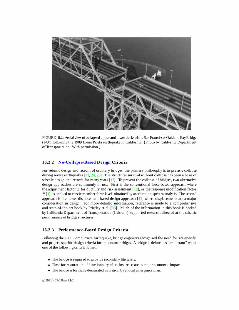
FIGURE16.2: Aerial viewofcollapsedupperand lowerdecksof theSanFrancisco-OaklandBayBridge(I-80) following the 1989 Loma Prieta earthquake in California. (Photo by California Departmentof Transportation. With permission.)

16.2.2 No-Collapse-Based Design Criteria

For seismic design and retrofit of ordinary bridges, the primary philosophy is to prevent collapseduring severe earthquakes [13, 24, 25]. The structural survival without collapse has been a basis ofseismic design and retrofit for many years [13]. To prevent the collapse of bridges, two alternativedesign approaches are commonly in use. First is the conventional force-based approach wherethe adjustment factor Z for ductility and risk assessment [12], or the response modification factorR [1], is applied to elastic member force levels obtained by acceleration spectra analysis. The secondapproach is the newer displacement-based design approach [13] where displacements are a majorconsideration in design. For more detailed information, reference is made to a comprehensiveand state-of-the-art book by Prietley et al. [35]. Much of the information in this book is backedby California Department of Transportation (Caltrans)-supported research, directed at the seismicperformance of bridge structures.

16.2.3 Performance-Based Design Criteria

Following the 1989 Loma Prieta earthquake, bridge engineers recognized the need for site-specificand project-specific design criteria for important bridges. A bridge is defined as “important” whenone of the following criteria is met:

• The bridge is required to provide secondary life safety.

• Time for restoration of functionality after closure creates a major economic impact.

• The bridge is formally designated as critical by a local emergency plan.


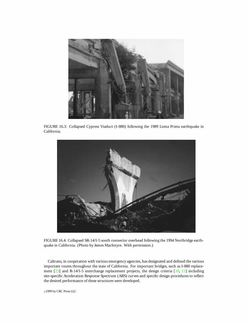
FIGURE 16.3: Collapsed Cypress Viaduct (I-880) following the 1989 Loma Prieta earthquake inCalifornia.

FIGURE 16.4: Collapsed SR-14/I-5 south connector overhead following the 1994 Northridge earth-quake in California. (Photo by James MacIntyre. With permission.)

Caltrans, in cooperation with various emergency agencies, has designated and defined the variousimportant routes throughout the state of California. For important bridges, such as I-880 replace-ment [23] and R-14/I-5 interchange replacement projects, the design criteria [10, 11] includingsite-specific Acceleration Response Spectrum (ARS) curves and specific design procedures to reflectthe desired performance of these structures were developed.


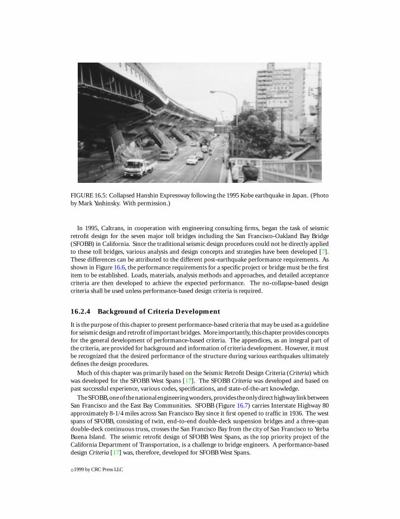
FIGURE 16.5: Collapsed Hanshin Expressway following the 1995 Kobe earthquake in Japan. (Photoby Mark Yashinsky. With permission.)

In 1995, Caltrans, in cooperation with engineering consulting firms, began the task of seismicretrofit design for the seven major toll bridges including the San Francisco-Oakland Bay Bridge(SFOBB) in California. Since the traditional seismic design procedures could not be directly appliedto these toll bridges, various analysis and design concepts and strategies have been developed [7].These differences can be attributed to the different post-earthquake performance requirements. Asshown in Figure 16.6, the performance requirements for a specific project or bridge must be the firstitem to be established. Loads, materials, analysis methods and approaches, and detailed acceptancecriteria are then developed to achieve the expected performance. The no-collapse-based designcriteria shall be used unless performance-based design criteria is required.

16.2.4 Background of Criteria Development

It is the purpose of this chapter to present performance-based criteria that may be used as a guidelinefor seismic design and retrofit of important bridges. More importantly, this chapter provides conceptsfor the general development of performance-based criteria. The appendices, as an integral part ofthe criteria, are provided for background and information of criteria development. However, it mustbe recognized that the desired performance of the structure during various earthquakes ultimatelydefines the design procedures.

Much of this chapter was primarily based on the Seismic Retrofit Design Criteria (Criteria) whichwas developed for the SFOBB West Spans [17]. The SFOBB Criteria was developed and based onpast successful experience, various codes, specifications, and state-of-the-art knowledge.

TheSFOBB,oneof thenational engineeringwonders, provides theonlydirecthighway linkbetweenSan Francisco and the East Bay Communities. SFOBB (Figure 16.7) carries Interstate Highway 80approximately 8-1/4 miles across San Francisco Bay since it first opened to traffic in 1936. The westspans of SFOBB, consisting of twin, end-to-end double-deck suspension bridges and a three-spandouble-deck continuous truss, crosses the San Francisco Bay from the city of San Francisco to YerbaBuena Island. The seismic retrofit design of SFOBB West Spans, as the top priority project of theCalifornia Department of Transportation, is a challenge to bridge engineers. A performance-baseddesign Criteria [17] was, therefore, developed for SFOBB West Spans.


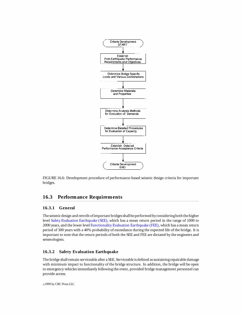
FIGURE 16.6: Development procedure of performance-based seismic design criteria for importantbridges.

16.3 Performance Requirements

16.3.1 General

The seismicdesignand retrofitof importantbridges shall beperformedbyconsideringboth thehigherlevel Safety Evaluation Earthquake (SEE), which has a mean return period in the range of 1000 to2000 years, and the lower level Functionality Evaluation Earthquake (FEE), which has a mean returnperiod of 300 years with a 40% probability of exceedance during the expected life of the bridge. It isimportant to note that the return periods of both the SEE and FEE are dictated by the engineers andseismologists.

16.3.2 Safety Evaluation Earthquake

The bridge shall remain serviceable after a SEE. Serviceable is defined as sustaining repairable damagewith minimum impact to functionality of the bridge structure. In addition, the bridge will be opento emergency vehicles immediately following the event, provided bridge management personnel canprovide access.


(a) West crossing spans.

(b) East crossing spans.

FIGURE 16.7: San Francisco-Oakland Bay Bridge. (Photo by California Department of Transporta-tion. With permission.)


16.3.3 Functionality Evaluation Earthquake

The bridge shall remain fully operational after a FEE. Fully operational is defined as full accessibilityto the bridge by current normal daily traffic. The structure may suffer repairable damage, butrepair operations may not impede traffic in excess of what is currently required for normal dailymaintenance.

16.3.4 Objectives of Seismic Design

The objectives of seismic design are as follows:

1. To keep the Critical structural components in the essentially elastic range during the SEE.

2. To achieve safety, reliability, serviceability, constructibility, and maintainability when theSeismic Response Modification Devices (SRMDs), i.e., energy dissipation and isolationdevices, are installed in bridges.

3. To devise expansion joint assemblies between bridge frames that either retain trafficsupport or, with the installation of deck plates, are able to carry the designated trafficafter being subjected to SEE displacements.

4. To provide ductile load paths and detailing to ensure bridge safety in the event that futuredemands might exceed those demands resulting from current SEE ground motions.

16.4 Loads and Load Combinations

16.4.1 Load Factors and Combinations

New and retrofitted bridge components shall be designed for the applicable load combinations inaccordance with the requirements of AASHTO-LRFD [1].

The load effect shall be obtained by

Load effect = η∑

γiQi (16.1)

whereQi = force effectη = a factor relating to ductility, redundancy, and operational importanceγi = load factor corresponding to Qi

.The AASHTO-LRFD load factors or load factors η = 1.0 and γi = 1.0 may be used for seismic

design.The live load on the bridge shall be determined by ADTT (Average Daily Truck Traffic) value for

the project. The bridge shall be analyzed for the worst case with or without live load. The mass of thelive loads shall not be included in the dynamic calculations. The intent of the live load combinationis to include the weight effect of the vehicles only.

16.4.2 Earthquake Load

The earthquake load – ground motions and response spectra shall be considered at two levels: SEEand FEE. The ground motions and response spectra may be generated in accordance with CaltransGuidelines [14, 15].


16.4.3 Wind Load

1. Wind load on structures — Wind loads shall be applied as a static equivalent load inaccordance with AASHTO-LRFD [1] .

2. Wind load on live load — Wind pressure on vehicles shall be represented by a uniformload of 0.100 kips/ft (1.46 kN/m) applied at right angles to the longitudinal axis of thestructure and 6.0 ft (1.85 m) above the deck to represent the wind load on vehicles.

3. Wind load dynamics — The expansion joints, SRMDs, and wind locks (tongues) shall beevaluated for the dynamic effects of wind loads.

16.4.4 Buoyancy and Hydrodynamic Mass

The buoyancy shall be considered to be an uplift force acting on all components below design waterlevel. Hydrodynamic mass effects [26] shall be considered for bridges over water.

16.5 Structural Materials

16.5.1 Existing Materials

For seismic retrofit design, aged concrete with specified strength of 3250 psi (22.4 MPa) can beconsidered to have a compressive strength of 5000 psi (34.5 MPa). If possible, cores of existingconcrete should be taken. Behavior of structural steel and reinforcement shall be based on millcertificate or tensile test results. If they are not available in bridge archives, a nominal strength of 1.1times specified yield strength may be used [13].

16.5.2 New Materials

Structural Steel

New structural steel used shall be AASHTO designation M270 (ASTM designation A709) Grade36 and Grade 50.

Welds shall be as specified in the Bridge Welding Code ANSI/AASHTO/AWS D1.5-95 [8].Partial penetrationwelds shall notbeused in regionsof structural components subjected topossible

inelastic deformation.High strength bolts conforming to ASTM designation A325 shall be used for all new connections

and forupgrading strengthsof existing riveted connections. Newbolted connections shall bedesignedas bearing-type for seismic loads and shall be slip-critical for all other load cases.

All bolts with a required length under the head greater than 8 in. shall be designated as ASTM A449threaded rods (requiring nuts at each end) unless a verified source of longer bolts can be identified.

New anchor bolts shall be designated as ASTM A449 threaded rods.

Structural Concrete

All concrete shall be normal weight concrete with the following properties:

Specified compressive strength: fcmin = 4, 000 psi (27.6MPa)Modulus of elasticity: Ec = 57,000

√f ′

c psi

Modulus of rupture: fr = 5√

f ′c psi

Reinforcement

All reinforcement shall use ASTM A706 (Grade 60) with the following specified properties:


Specified minimum yield stress: Fy = 60ksi (414MPa)Specified minimum tensile strength: Fu = 90ksi (621MPa)Specified maximum yield stress: Fymax = 78ksi (538MPa)Specified maximum tensile strength: Fumax = 107ksi (738MPa)Modulus of elasticity: Es = 29,000ksi (200,000MPa)

Strain hardening strain: εsh =

0.0150 for #8and smallers bars0.0125 for #90.0100 for #10and #110.0075 for #140.0050 for #18

16.6 Determination of Demands

16.6.1 Analysis Methods

Static Linear Analysis

Static linear analysis shall be used to determine member forces due to self weight, wind, watercurrents, temperature, and live load.

Dynamic Response Spectrum Analysis

1. Dynamic response spectrum analysis shall be used for the local and regional stand alonemodels and the simplified global model described in Section 16.6.2 to determine modeshapes, structure periods, and initial estimates of seismic force and displacement de-mands.

2. Dynamic response spectrum analysis may be used on global models prior to time historyanalysis to verify model behavior and eliminate modeling errors.

3. Dynamic response spectrum analysis may be used to identify initial regions or membersof likely inelastic behavior which need further refined analysis using inelastic nonlinearelements.

4. Site specific ARS curves shall be used, with 5% damping.

5. Modal responses shall be combined using the Complete Quadratic Combination (CQC)method and the resulting orthogonal responses shall be combined using either the SquareRoot of the Sum of the Squares (SRSS) method or the “30%” rule, e.g., RH = Max(Rx +0.3Ry, Ry + 0.3Rx) [13].

6. Due to the expected levels of inelastic structural response in some members and regions,dynamic response spectrum analysis shall not be used to determine final design demandvalues or to assess the performance of the retrofitted structures.

Dynamic Time History Analysis

Site specific multi-support dynamic time histories shall be used in a dynamic time historyanalysis. All analyses incorporating significant nonlinear behavior shall be conducted using nonlinearinelastic dynamic time history procedures.

1. Linear elasticdynamic timehistory analysis—Linear elasticdynamic timehistory analysisis defined as dynamic time history analysis with considerations of geometrical linearity


(small displacement), linear boundary conditions, and elastic members. It shall only beused to check regional and global models.

2. Nonlinearelasticdynamic timehistoryanalysis—Nonlinearelastic timehistoryanalysis isdefined as dynamic time history analysis with considerations of geometrical nonlinearity,linear boundary conditions, and elastic members. It shall be used to determine areas ofinelastic behavior prior to incorporating inelasticity into the regional and global models.

3. Nonlinear inelastic dynamic time history analysis – Level I — Nonlinear inelastic dy-namic time history analysis – Level I is defined as dynamic time history analysis withconsiderations of geometrical nonlinearity, nonlinear boundary conditions, other inelas-tic elements (for example, dampers) and elastic members. It shall be used for the finaldetermination of force and displacement demands for existing structures in combinationwith static gravity, wind, thermal, water current, and live load as specified in Section 16.4.

4. Nonlinear inelastic dynamic time history analysis – Level II — Nonlinear inelastic dy-namic time history analysis – Level II is defined as dynamic time history analysis withconsiderations of geometrical nonlinearity, nonlinear boundary conditions, other inelas-tic elements (for example, dampers) and inelastic members. It shall be used for the finalevaluation of response of the structures. Reduced material and section properties, and theyield surface equation suggested in the Appendix may be used for inelastic considerations.

16.6.2 Modeling Considerations

Global, Regional, and Local Models

The global models focus on the overall behavior and may include simplifications of complexstructural elements. Regional models concentrate on regional behavior. Local models emphasizethe localized behavior, especially complex inelastic and nonlinear behavior. In regional and globalmodels where more than one foundation location is included in the model, multi-support timehistory analysis shall be used.

Boundary Conditions

Appropriate boundary conditions shall be included in the regional models to represent theinteraction between the regional model and the adjacent portion of the structure not explicitlyincluded. The adjacent portion not specifically included may be modeled using simplified structuralcombinations of springs, dashpots, and lumped masses.

Appropriate nonlinear elements such as gap elements, nonlinear springs, SRMDs, or specializednonlinear finite elements shall be included where the behavior and response of the structure isdetermined to be sensitive to such elements.

Soil-Foundation-Structure-Interaction

Soil-Foundation-Structure-Interactionmaybe consideredusingnonlinearorhysteretic springsin the global and regional models. Foundation springs at the base of the structure which reflect thedynamic properties of the supporting soil shall be included in both regional and global models.

Section Properties of Latticed Members

For latticed members, the procedure proposed in the

Appendix may be used for member characterization.


Damping

When nonlinear member properties are incorporated in the model, Rayleigh damping shall bereduced, for example by 20%, compared with analysis with elastic member properties.

Seismic Response Modification Devices

The SRMDs, i.e., energy dissipation and isolation devices, shall be modeled explicitly usingtheir hysteretic characteristics as determined by tests.

16.7 Determination of Capacities

16.7.1 Limit States and Resistance Factors

Limit States

The limit states are defined as those conditions of a structure at which it ceases to satisfy theprovisions for which it was designed. Two kinds of limit states corresponding to SEE and FEE specifiedin Section 16.3 apply for seismic design and retrofit.

Resistance Factors

To account for unavoidable inaccuracies in the theory, variation in the material properties,workmanship, and dimensions, nominal strength of structural components should be modified bya resistance factor φ to obtain the design capacity or strength (resistance). The following resistancefactors shall be used for seismic design:

• For tension fracture in net section φtf = 0.8• For block shear φbs = 0.8• For bolts and welds φ = 0.8• For all other cases φ = 1.0

16.7.2 Effective Length of Compression Members

Theeffective length factor K for compressionmembers shall bedetermined inaccordancewithChap-ter 17 of this Handbook.

16.7.3 Nominal Strength of Steel Structures

Members

1. General — Steel members include rolled members and built-up members, such as lat-ticed, battened, and perforated members. The design strength of those members shallbe according to applicable provisions of AISC-LRFD [4]. Section properties of latticedmembers shall be determined in accordance with the Appendix.

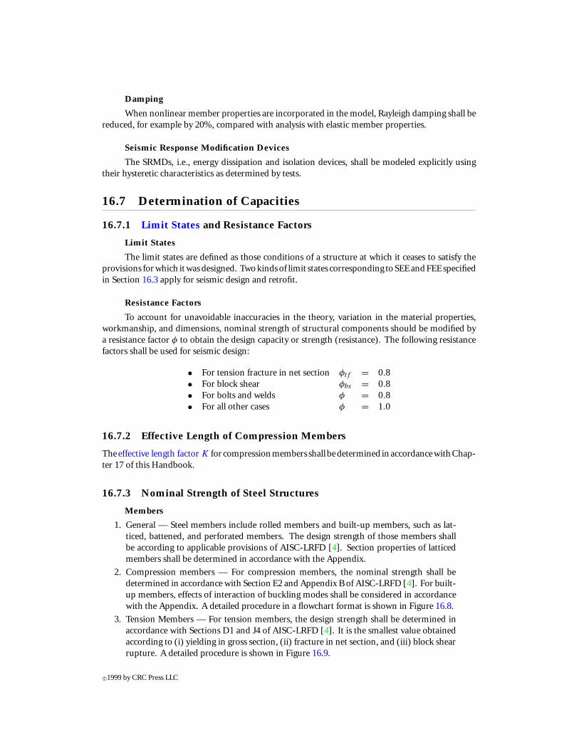
2. Compression members — For compression members, the nominal strength shall bedetermined in accordance with Section E2 and Appendix B of AISC-LRFD [4]. For built-up members, effects of interaction of buckling modes shall be considered in accordancewith the Appendix. A detailed procedure in a flowchart format is shown in Figure 16.8.

3. Tension Members — For tension members, the design strength shall be determined inaccordance with Sections D1 and J4 of AISC-LRFD [4]. It is the smallest value obtainedaccording to (i) yielding in gross section, (ii) fracture in net section, and (iii) block shearrupture. A detailed procedure is shown in Figure 16.9.


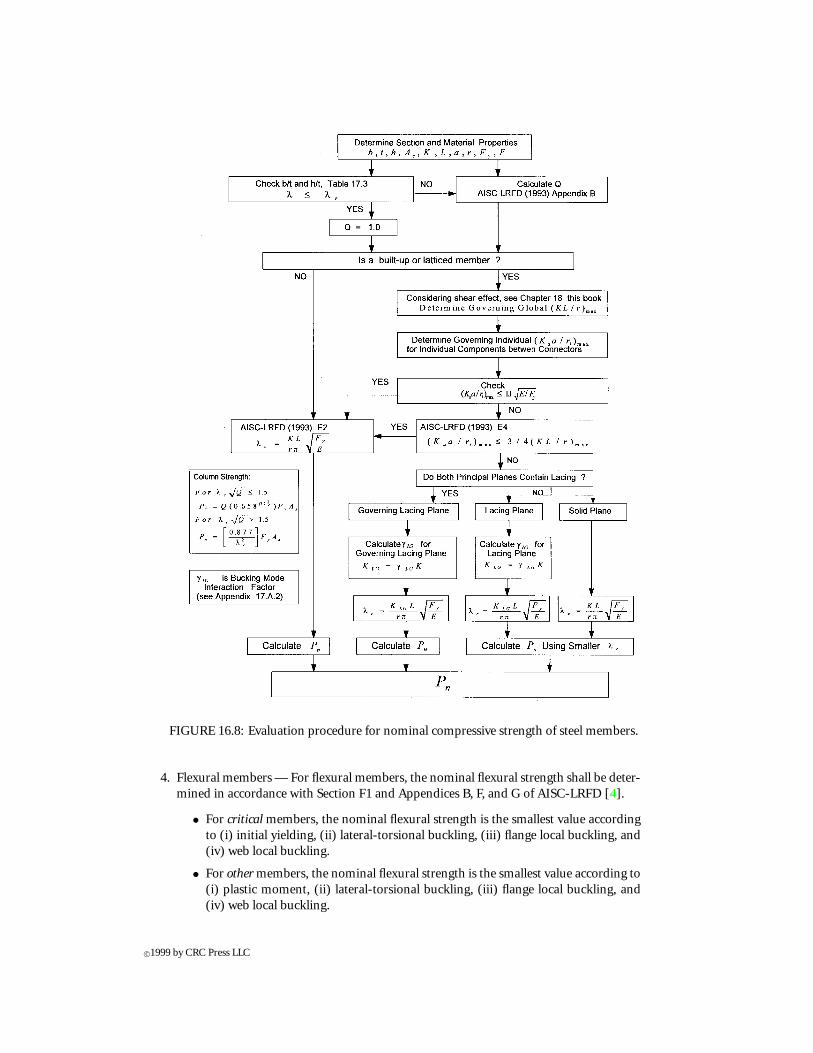
FIGURE 16.8: Evaluation procedure for nominal compressive strength of steel members.

4. Flexural members — For flexural members, the nominal flexural strength shall be deter-mined in accordance with Section F1 and Appendices B, F, and G of AISC-LRFD [4].

• For critical members, the nominal flexural strength is the smallest value accordingto (i) initial yielding, (ii) lateral-torsional buckling, (iii) flange local buckling, and(iv) web local buckling.

• For other members, the nominal flexural strength is the smallest value according to(i) plastic moment, (ii) lateral-torsional buckling, (iii) flange local buckling, and(iv) web local buckling.


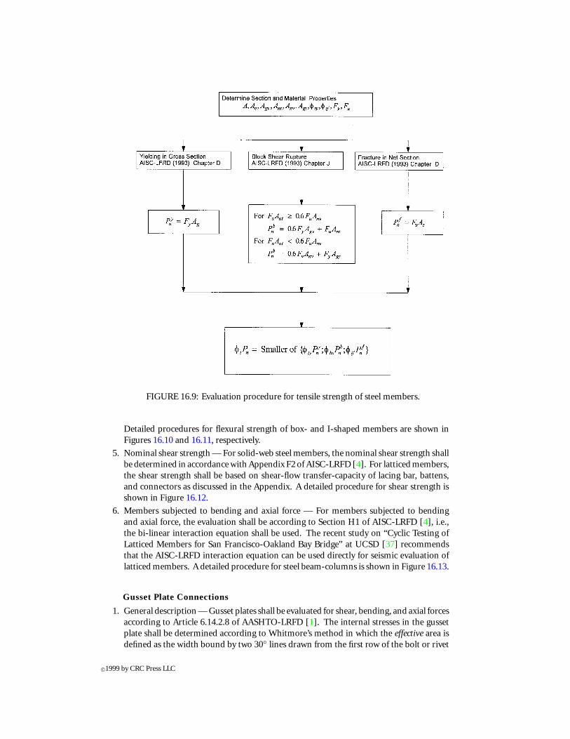
FIGURE 16.9: Evaluation procedure for tensile strength of steel members.

Detailed procedures for flexural strength of box- and I-shaped members are shown inFigures 16.10 and 16.11, respectively.

5. Nominal shear strength — For solid-web steel members, the nominal shear strength shallbe determined in accordance with Appendix F2 of AISC-LRFD [4]. For latticed members,the shear strength shall be based on shear-flow transfer-capacity of lacing bar, battens,and connectors as discussed in the Appendix. A detailed procedure for shear strength isshown in Figure 16.12.

6. Members subjected to bending and axial force — For members subjected to bendingand axial force, the evaluation shall be according to Section H1 of AISC-LRFD [4], i.e.,the bi-linear interaction equation shall be used. The recent study on “Cyclic Testing ofLatticed Members for San Francisco-Oakland Bay Bridge” at UCSD [37] recommendsthat the AISC-LRFD interaction equation can be used directly for seismic evaluation oflatticed members. A detailed procedure for steel beam-columns is shown in Figure 16.13.

Gusset Plate Connections

1. General description — Gusset plates shall be evaluated for shear, bending, and axial forcesaccording to Article 6.14.2.8 of AASHTO-LRFD [1]. The internal stresses in the gussetplate shall be determined according to Whitmore’s method in which the effective area isdefined as the width bound by two 30◦ lines drawn from the first row of the bolt or rivet


FIGURE 16.10: Evaluation procedure for nominal flexural strength of box-shaped steel members.

group to the last bolt or rivet line. The stresses in the gusset plate may be determined bymore rational methods or refined computer models.

2. Tension strength — The tension capacity of the gusset plates shall be calculated accordingto Article 6.13.5.2 of AASHTO-LRFD [1].

3. Compressive strength — The compression capacity of the gusset plates shall be calcu-lated according to Article 6.9.4.1 of AASHTO-LRFD [1]. In using the AASHTO-LRFDEquations (6.9.4.1-1) and (6.9.4.1-2), symbol l is the length from the last rivet (or bolt)line on a member to first rivet (or bolt) line on a chord measured along the centerline ofthe member; K is effective length factor = 0.65; As is average effective cross-section areadefined by Whitmore’s method.

4. Limit of free edge to thickness ratio of gusset plate — When the free edge length tothickness ratio of a gusset plate Lg/t > 1.6

√E/Fy , the compression stress of a gusset

plate shall be less than 0.8 Fy ; otherwise the plate shall be stiffened. The free edge lengthto thickness ratio of a gusset plate shall satisfy the following limit specified in Article6.14.2.8 of AASHTO-LRFD [1].

Lg

t≤ 2.06

√E

Fy

(16.2)

When the free edge is stiffened, the following requirements shall be satisfied:

• The stiffener plus a width of 10t of gusset plate shall have an l/r ratio less than orequal to 40.


FIGURE 16.11: Evaluation procedure for nominal flexural strength of I-shaped steel members.

• The stiffener shall have an l/r ratio less than or equal to 40 between fasteners.

• The stiffener moment of inertia shall satisfy [38]:

Is ≥{

1.83t4√

(b/t)2 − 1449.2t4

(16.3)

where

Is = the moment of inertia of the stiffener about its own centroid

b = the width of the gusset plate perpendicular to the edge

t = the thickness of the gusset plate

5. In-plane moment strength of gusset plate (strong axis) — The nominal moment strengthof a gusset plate shall be calculated by the following equation in Article 6.14.2.8 ofAASHTO-LRFD [1]:

Mn = SFy (16.4)

whereS = elastic section modulus about the strong axis

6. In-plane shear strength for a gusset plate — The nominal shear strength of a gusset plateshall be calculated by the following equations:


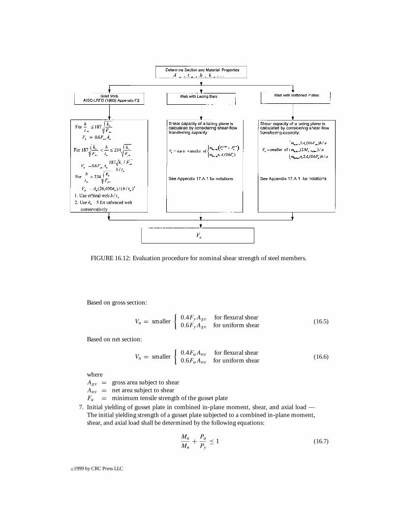
FIGURE 16.12: Evaluation procedure for nominal shear strength of steel members.

Based on gross section:

Vn = smaller

{0.4FyAgv for flexural shear0.6FyAgv for uniform shear

(16.5)

Based on net section:

Vn = smaller

{0.4FuAnv for flexural shear0.6FuAnv for uniform shear

(16.6)

whereAgv = gross area subject to shearAnv = net area subject to shearFu = minimum tensile strength of the gusset plate

7. Initial yielding of gusset plate in combined in-plane moment, shear, and axial load —The initial yielding strength of a gusset plate subjected to a combined in-plane moment,shear, and axial load shall be determined by the following equations:

Mu

Mn

+ Pu

Py

≤ 1 (16.7)


FIGURE 16.13: Evaluation procedure for steel beam-columns.

or (Vu

Vn

)2

+(

Pu

Py

)2

≤ 1 (16.8)

whereVu = factored shearMu = factored momentPu = factored axial loadMn = nominal moment strength determined by Equation 16.4Vn = nominal shear strength determined by Equation 16.5Py = yield axial strength (AgFy)

Ag = gross section area of gusset plate

8. Full yielding of gusset plate in combined in-plane moment, shear, and axial load — Fullyielding strength for a gusset plate subjected to combined in-plane moment, shear, andaxial load has the form [6]:


Mu

Mp

+(

Pu

Py

)2

+(

Vu

Vp

)4

[1 −

(Pu

Py

)2] = 1 (16.9)

whereMp = plastic moment of pure bending (ZFy)

Vp = shear capacity of gusset plate (0.6AgFy)

Z = plastic section modulus

9. Block shear capacity — The block shear capacity shall be calculated according to Article6.13.4 of AASHTO-LRFD [1].

10. Out-of-plane moment and shear consideration — Moment will be resolved into a coupleacting on the near and far side gusset plates. This will result in tension or compressionon the respective plates. This force will produce weak axis bending of the gusset plate.

Connections Splices

The splice section shall be evaluated for axial tension, flexure, and combined axial and flexuralloading cases according to AISC-LRFD [4]. The member splice capacity shall be equal to or greaterthan the capacity of the smaller of the two members being spliced.

Eyebars

The tensile capacity of the eyebars shall be calculated according to Article D3 of AISC-LRFD [4].

Anchor Bolts (Rods) and Anchorage Assemblies

1. Anchorage assemblies for nonrocking mechanisms shall be anchored with sufficient ca-pacity todevelop the lesserof the seismic forcedemandandplastic strengthof thecolumns.Anchorage assemblies may be designed for rocking mechanisms where yield is permitted— at which point rocking commences. Shear keys shall be provided to prevent excess lat-eral movement. The nominal shear strength of pipe guided shear keys shall be calculatedby:

Rn = 0.6FyAp (16.10)

whereAp = cross-section area of pipe

2. Evaluation of anchorage assemblies shall be based on reinforced concrete structure be-havior with bonded or unbonded anchor rods under combined axial load and bendingmoment. All anchor rods outside of the compressive region may be taken to full minimumtensile strength.

3. The nominal strength of anchor bolts (rods) for shear, tension, and combined shear andtension shall be calculated according to Article 6.13.2 of AASHTO-LRFD [1].

4. Embedment length of anchor rods shall be such that a ductile failure occurs. Concretefailure surfaces shall be based on a shear stress of 2

√f ′

c and account for edge distancesand overlapping shear zones. In no case should edge distances or embedments be lessthan those shown in Table 8-26 of the AISC-LRFD Manual [3]. New anchor rods shallbe threaded to assure development.


Rivets and Holes

1. The bearing capacity on rivet holes shall be calculated according to Article 6.13.2.9 ofAASHTO-LRFD [1].

2. Nominal shear strength of a rivet shall be calculated by the following formula:

Rn = 0.75βFuArNs (16.11)

whereβ = 0.8, reduction factor for connections with more than two rivets and to account

for deformation of connected material which causes nonuniform rivet shear force(see Article C6.13.2.7 of AASHTO-LRFD [1])

Fu = minimum tensile strength of the rivetAr = the nominal area of the rivet (before driving)Ns = number of shear planes per rivetIt should be pointed out that the 0.75 factor is the ratio of the shear strength τu to thetensile strength Fu of a rivet. The research work by Kulak et al. [31] found that this ratiois independent of the rivet grade, installation procedure, diameter, and grip length and isabout 0.75.

3. Tension capacity of a rivet shall be calculated by the following formula:

Tn = ArFu (16.12)

4. Tensile capacity of a rivet subjected to combined tension and shear shall be calculated bythe following formula:

Tn = ArFu

√1 − Vu

Rn

(16.13)

whereVu = factored shear forceRn = nominal shear strength of a rivet determined by Equation 16.11

Bolts and Holes

1. The bearing capacity on bolt holes shall be calculated according to Article 6.13.2.9 ofAASHTO-LRFD [1].

2. The nominal strength of a bolt for shear, tension, and combined shear and tension shallbe calculated according to Article 6.13.2 of AASHTO-LRFD [1].

Prying Action

Additional tension forces resulting from prying action must be accounted for in determiningapplied loads on rivets or bolts. The connected elements (primarily angles) must also be checked foradequate flexural strength. Prying action forces shall be determined from the equations presented inAISC-LRFD Manual Volume 2, Part 11 [3].


16.7.4 Nominal Strength of Concrete Structures

Nominal Moment Strength

The nominal moment strengthMn shall be calculated by considering combined biaxial bendingand axial loads. It is defined as:

Mn = smaller

{My

Mεc(16.14)

whereMy = moment corresponding to first steel yieldMεc = moment at which compressive strain of concrete at extreme fiber equal to 0.003

Nominal Shear Strength

The nominal shear strength Vn shall be calculated by the following equations [12, 13].

Vn = Vc + Vs (16.15a)

or Vn = Vc + Vt (16.15b)

Vc = 0.8νcAg (16.16)

νc = larger

2(1 + Pu

2,000Ag

) √f ′

c ≤ 3√

f ′c

Factor 1 ×(1 + Pu

2,000Ag

) √f ′

c ≤ 4√

f ′c

(16.17)

Factor 1 = ρ′′fyt

150+ 3.67− µ1 ≤ 3.0

ρ′′ = volume of transverse reinforcement

volume of confined core(16.18)

Vs =

Aνfytd/s for rectangular sections

AsfytD′

2sfor circular sections

(16.19)

whereAg = gross section area of concrete memberAs = cross-sectional area of transverse reinforcement within space s

Vt = shear strength carried by truss mechanismD′ = hoop or spiral diameterPu = factored axial load associated with design shear Vu and Pu/Ag is in psid = effective depth of sections = space of transverse reinforcementfyt = probable yield strength of transverse steel (psi)µ1 = ductility demand ratio (1.0 will be used)

16.7.5 Structural Deformation Capacity

Steel Structures

Displacement capacity shall be evaluated by considering both material and geometrical non-linearity. Proper boundary conditions for various structures shall be carefully adjusted. The ultimate


available displacement capacity is defined as the displacement corresponding to a load that drops amaximum of 20% from the peak load.

Reinforced Concrete Structures

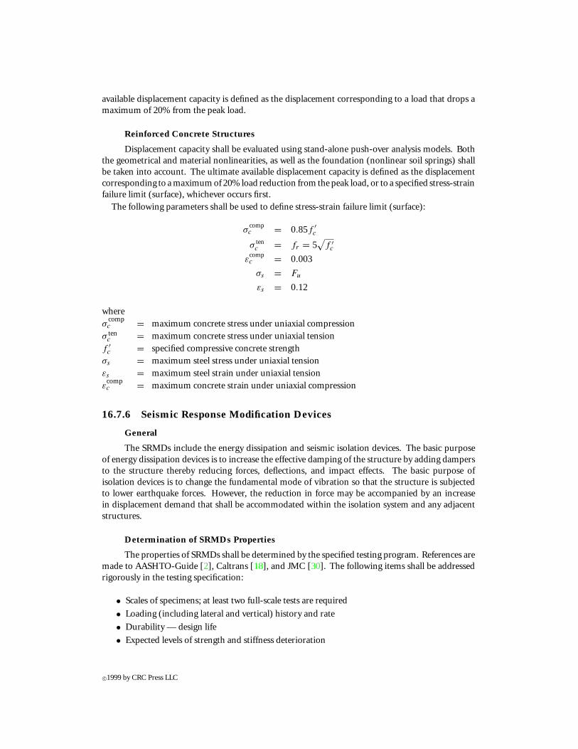
Displacement capacity shall be evaluated using stand-alone push-over analysis models. Boththe geometrical and material nonlinearities, as well as the foundation (nonlinear soil springs) shallbe taken into account. The ultimate available displacement capacity is defined as the displacementcorresponding to a maximum of 20% load reduction from the peak load, or to a specified stress-strainfailure limit (surface), whichever occurs first.

The following parameters shall be used to define stress-strain failure limit (surface):

σcompc = 0.85f ′

c

σ tenc = fr = 5

√f ′

c

εcompc = 0.003

σs = Fu

εs = 0.12

whereσ

compc = maximum concrete stress under uniaxial compression

σ tenc = maximum concrete stress under uniaxial tension

f ′c = specified compressive concrete strength

σs = maximum steel stress under uniaxial tensionεs = maximum steel strain under uniaxial tensionε

compc = maximum concrete strain under uniaxial compression

16.7.6 Seismic Response Modification Devices

General

The SRMDs include the energy dissipation and seismic isolation devices. The basic purposeof energy dissipation devices is to increase the effective damping of the structure by adding dampersto the structure thereby reducing forces, deflections, and impact effects. The basic purpose ofisolation devices is to change the fundamental mode of vibration so that the structure is subjectedto lower earthquake forces. However, the reduction in force may be accompanied by an increasein displacement demand that shall be accommodated within the isolation system and any adjacentstructures.

Determination of SRMDs Properties

The properties of SRMDs shall be determined by the specified testing program. References aremade to AASHTO-Guide [2], Caltrans [18], and JMC [30]. The following items shall be addressedrigorously in the testing specification:

• Scales of specimens; at least two full-scale tests are required

• Loading (including lateral and vertical) history and rate

• Durability — design life

• Expected levels of strength and stiffness deterioration


16.8 Performance Acceptance Criteria

16.8.1 General

To achieve the performance objectives stated in Section 16.3, the various structural components shallsatisfy the acceptable demand/capacity ratios, DCaccept, specified in this section. The general designformat is given by the formula:

Demand

Capacity≤ DCaccept (16.20)

wheredemand, in termsof various factored forces (moment, shear, axial force, etc.), anddeformations(displacement, rotation, etc.) shall be obtained by the nonlinear inelastic dynamic time historyanalysis – Level I defined in Section 16.6; and capacity, in terms of factored strength and deformations,shall be obtained according to the provisions set forth in Section 16.7. For members subjected tocombined loadings, the definition of force D/C ratio:] D/C ratios is given in the Appendix.

16.8.2 Structural Component Classifications

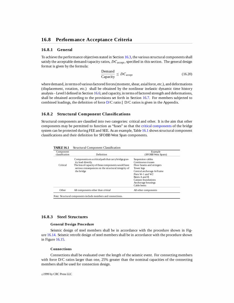
Structural components are classified into two categories: critical and other. It is the aim that othercomponents may be permitted to function as “fuses” so that the critical components of the bridgesystem can be protected during FEE and SEE. As an example, Table 16.1 shows structural componentclassifications and their definition for SFOBB West Span components.

TABLE 16.1 Structural Component ClassificationComponent Exampleclassification Definition (SFOBB West Spans)

Componentsonacriticalpath that carrybridgegrav-ity load directly.

Suspension cablesContinuous trusses

Critical The loss of capacity of these components would haveserious consequences on the structural integrity ofthe bridge

Floor beams and stringersTower legsCentral anchorage A-FramePiers W-1 and W2Bents A and BCaisson foundationsAnchorage housingsCable bents

Other All components other than critical All other components

Note: Structural components include members and connections.

16.8.3 Steel Structures

General Design Procedure

Seismic design of steel members shall be in accordance with the procedure shown in Fig-ure 16.14. Seismic retrofit design of steel members shall be in accordance with the procedure shownin Figure 16.15.

Connections

Connections shall be evaluated over the length of the seismic event. For connecting memberswith force D/C ratios larger than one, 25% greater than the nominal capacities of the connectingmembers shall be used for connection design.


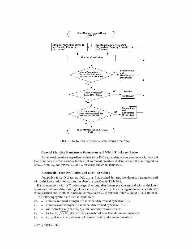
FIGURE 16.14: Steel member seismic design procedure.

General Limiting Slenderness Parameters and Width-Thickness Ratios

For all steel members regardless of their force D/C ratios, slenderness parameters λc for axialload dominant members, and λb for flexural dominant members shall not exceed the limiting values(0.9λcr or 0.9λbr for critical, λcr or λbr for other) shown in Table 16.2.

Acceptable Force D/C Ratios and Limiting Values

Acceptable force D/C ratios, DCaccept and associated limiting slenderness parameters andwidth-thickness ratios for various members are specified in Table 16.2.

For all members with D/C ratios larger than one, slenderness parameters and width- thicknessratios shall not exceed the limiting values specified in Table 16.2. For existing steel members with D/Cratios less than one, width-thickness ratios may exceed λr specified in Table 16.3 and AISC-LRFD [4].

The following symbols are used in Table 16.2:Mn = nominal moment strength of a member determined by Section 16.7Pn = nominal axial strength of a member determined by Section 16.7λ = width-thickness (b/t or h/tw) ratio of compressive elementsλc = (KL/rπ)

√Fy/E, slenderness parameter of axial load dominant members

λb = L/ry , slenderness parameter of flexural moment dominant members


FIGURE 16.15: Steel member seismic retrofit design procedure.

TABLE 16.2 Acceptable Force Demand/Capacity Ratios and Limiting

Slenderness Parameters and Width/Thickness RatiosLimiting ratios Acceptable

Slenderness Width/thickness forceparameter λ D/C ratio

Member classification (λc and λb) (b/t or h/tw) D/Caccept

Axial load 0.9 λcr λr DCr = 1.0

dominant λcpr λpr 1.0 ∼ 1.2

Pu/Pn ≥ Mu/Mn λcp λp DCp = 1.2

Critical Flexural moment 0.9 λbr λr DCr = 1.0

dominant λbpr λpr 1.2 ∼ 1.5

Mu/Mn > Pu/Pn λbp λp DCp = 1.5

Axial load λcr λr DCr = 1.0

dominant λcpr λpr 1.0 ∼ 2.0

Pu/Pn ≥ Mu/Mn λcp λp−Seismic DCp = 2

Other Flexural moment λbr λr DCr = 1.0

dominant λbpr λpr 1.0 ∼ 2.5

Mu/Mn > Pu/Pn λbp λp−Seismic DCp = 2.5


TABLE 16.3 Limiting Width-Thickness Ratio


λcp = 0.5, limiting column slenderness parameter for 90% of the axial yield load based on AISC-LRFD [4] column curve

λbp = limiting beam slenderness parameter for plastic moment for seismic designλcr = 1.5, limiting column slenderness parameter for elastic buckling based on AISC-LRFD [4]

column curveλbr = limiting beam slenderness parameter for elastic lateral torsional buckling

λbr =

57,000√

JAMr

for solid rectangular bars and box sections

X1FL

√1 +

√1 + X2F

2L for doubly symmetric I-shaped members and channels

Mr ={

FLSx for I-shaped member

Fyf Sx for solid rectangular and box section

X1 = π

Sx

√EGJA

2; X2 = 4Cw

Iy

(Sx

GJ

)2

; FL = smaller

{Fyw

Fyf − Fr

whereA = cross-sectional area, in.2

L = unsupported length of a memberJ = torsional constant, in.4

r = radius of gyration, in.ry = radius of gyration about minor axis, in.Fyw = yield stress of web, ksiFyf = yield stress of flange, ksiE = modulus of elasticity of steel (29,000ksi)G = shear modulus of elasticity of steel (11,200ksi)Sx = section modulus about major axis, in.3

Iy = moment of inertia about minor axis, in.4

Cw = warping constant, in.6

For doubly symmetric and singly symmetric I-shaped members with compression flange equal to orlarger than the tension flange, including hybrid members (strong axis bending):

λbp =

[3,600+2,200(M1/M2)]Fy

for other members300√Fyf

for critical members(16.21)

in whichM1 = larger moment at end of unbraced length of beamM2 = smaller moment at end of unbraced length of beam(M1/M2) = positive when moments cause reverse curvature and negative for single curvature

For solid rectangular bars and symmetric box beam (strong axis bending):

λbp ={ [5,000+3,000(M1/M2)]

Fy≥ 3,000

Fyfor other members

3,750Mp

√JA for critical members

(16.22)

in whichMp = plastic moment (ZxFy)Zx = plastic section modulus about major axis


FIGURE 16.16: Typical cross-sections for steel members (SFOBB west spans).

λr, λp, λp−Seismic are limiting width thickness ratios specified by Table 16.3

λpr =

[λp + (

λr − λp

) (DCp−DCaccept

DCp−DCr

)]for critical members[

λp−Seismic + (λr − λp−Seismic

) (DCp−DCaccept

DCp−DCr

)]for other members

(16.23)

For axial load dominant members (Pu/Pn ≥ Mu/Mn)

λcpr =

λcp + (0.9λcr − λcp

) (DCp−DCaccept

DCp−DCr

)for critical members

λcp + (λcr − λcp

) (DCp−DCaccept

DCp−DCr

)for other members

(16.24)

For flexural moment dominant members (Mu/Mn > Pu/Pn)

λbpr =

λbp + (0.9λbr − λbp

) (DCp−DCaccept

DCp−DCr


λbp + (λbr − λbp

) (DCp−DCaccept

DCp−DCr

)for other members

(16.25)


16.8.4 Concrete Structures

General

For all concrete compression members regardless of their force D/C ratios, slenderness param-eters KL/r shall not exceed 60.

For critical components, force DCaccept = 1.2 and deformation DCaccept = 0.4.

For other components, force DCaccept = 2.0 and deformation DCaccept = 0.67.

Beam-Column (Bent Cap) Joints

For concrete box girder bridges, the beam-column (bent cap) joints shall be evaluated anddesigned in accordance with the following guidelines [16, 40]:

1. Effective Superstructure Width — The effective width of a superstructure (box girder)on either side of a column to resist longitudinal seismic moment at bent (support) shallnot be taken as larger than the superstructure depth.

• The immediately adjacent girder on either side of a column within the effectivesuperstructure width is considered effective.

• Additional girders may be considered effective if refined bent-cap torsional analysisindicates that the additional girders can be mobilized.

2. Minimum Bent-Cap Width — Minimum cap width outside the column shall not be lessthan D/4 (D is column diameter or width in that direction) or 2 ft (0.61 m).

3. Acceptable Joint Shear Stress

• For existing unconfined joints, acceptable principal tensile stress shall be taken as3.5

√f ′

c psi (0.29√

f ′c MPa). If the principal tensile stress demand exceeds this

value, the joint shear reinforcement specified in (4) shall be provided.

• For new joints, acceptable principal tensile stress shall be taken as 12√

f ′c psi (1.0√

f ′c MPa).

• For existing and new joints, acceptable principal compressive stress shall be takenas 0.25 f ′

c .

4. Joint Shear Reinforcement

• Typical flexure and shear reinforcement (see Figures 16.17 and 16.18) in bent capsshall be supplemented in the vicinity of columns to resist joint shear. All joint shearreinforcement shall be well distributed and provided within D/2 from the face ofcolumn.

• Vertical reinforcement including cap stirrups and added bars shall be 20% ofthe column reinforcement anchored into the joint. Added bars shall be hookedaround main longitudinal cap bars. Transverse reinforcement in the joint regionshall consist of hoops with a minimum reinforcement ratio of 0.4 (column steelarea)/(embedment length of column bar into the bent cap)2.

• Horizontal reinforcement shall be stitched across the cap in two or more interme-diate layers. The reinforcement shall be shaped as hairpins, spaced vertically at notmore than 18 in. (457 mm). The hairpins shall be 10% of column reinforcement.Spacing shall be denser outside the column than that used within the column.

• Horizontal side face reinforcement shall be 10% of the main cap reinforcementincluding top and bottom steel.


FIGURE 16.17: Example cap joint shear reinforcement — skews 0◦ to 20◦.

• For bent caps skewed greater than 20◦, the vertical J-bars hooked around longitudi-nal deck and bent cap steel shall be 8% of the column steel (see Figure 16.18). TheJ-bars shall be alternatively 24 in. (600 mm) and 30 in. (750 mm) long and placedwithin a width of the column dimension on either side of the column centerline.

• All vertical column bars shall be extended as high as practically possible withoutinterfering with the main cap bars.

16.8.5 Seismic Response Modification Devices

General

Analysis methods specified in Section 16.6 shall apply for determining seismic design forcesand displacements on SRMDs. Properties or capacities of SRMDs shall be determined by specifiedtests.

Acceptance Criteria

SRMDs shall be able to perform their intended function and maintain their design parametersfor the design life (for example, 40 years) and for an ambient temperature range (for example from 30◦


FIGURE 16.18: Example cap joint shear reinforcement — skews > 20◦.

to 125◦F). The devices shall have accessibility for periodic inspections, maintenance, and exchange.In general, the SRMDs shall satisfy at least the following requirements:

• To remain stable and provide increasing resistance with the increasing displacement.Stiffness degradation under repeated cyclic load is unacceptable.

• To dissipate energy within the design displacement limits. For example: provisions maybe made to limit the maximum total displacement imposed on the device to preventdevice displacement failure, or the device shall have a displacement capacity 50% greaterthan the design displacement.

• To withstand or dissipate the heat build-up during reasonable seismic displacement timehistory.

• To survive for the number of cycles of displacement expected under wind excitationduring the life of the device and to function at maximum wind force and displacementlevels for at least, for example, five hours.


Defining Terms

Bridge: A structure that crosses over a river, bay, or other obstruction, permitting the smoothand safe passage of vehicles, trains, and pedestrians.

Buckling model interaction: A behavior phenomenon of compression built-up member; thatis, interaction between the individual (or local) buckling mode and the global bucklingmode.

Built-up member: A member made of structural metal elements that are welded, bolted, and/orriveted together.

Capacity: factored strength and deformation capacity obtained according to specified provi-sions.

Critical components: Structural components on a critical path that carry bridge gravity loaddirectly. The loss of capacity of these components would have serious consequences onthe structural integrity of the bridge.

Damage index: A ratio of elastic displacement demand to ultimate displacement.

D/C ratio: A ratio of demand to capacity.

Demands: In terms of various forces (moment, shear, axial force, etc.) and deformation (dis-placement, rotation, etc.) obtained by structural analysis.

Ductility: A nondimensional factor, i.e., ratio of ultimate deformation to yield deformation.

Effective length factor K : A factor that when multiplied by actual length of the end-restrainedcolumn gives the length of an equivalent pin-ended column whose elastic buckling loadis the same as that of the end-restrained column

Functionality evaluation earthquake (FEE): An earthquake that has a mean return period of300 years with a 40% probability of exceedance during the expected life of the bridge.

Latticed member: A member made of metal elements that are connected by lacing bars andbatten plates.

LRFD (Load and Resistance Factor Design): A method of proportioning structural compo-nents (members, connectors, connecting elements, and assemblages) such that no ap-plicable limit state is exceeded when the structure is subjected to all appropriate loadcombinations.

Limit states: Those conditions of a structure at which it ceases to satisfy the provision for whichit was designed.

No-collapse-based design: Design that is based on survival limit state. The overall designconcern is to prevent the bridge from catastrophic collapse and to save lives.

Other components: All components other than critical.

Performance-based seismic design: Design that is based on bridge performance requirements.The design philosophy is to accept some repairable earthquake damage and to keep bridgefunctional performance after earthquakes.

Safety evaluation earthquake (SEE): An earthquake that has a mean return period in the rangeof 1000 to 2000 years.

Seismic design: Design and analysis considering earthquake loads.

Seismic response modification devices (SRMDs): Seismic isolation and energy dissipation de-vices including isolators, dampers, or isolation/dissipation (I/D) devices.

Ultimate deformation: Deformation refers to a loading state at which structural system or astructural member can undergo change without losing significant load-carrying capacity.


The ultimate deformation is usually defined as the deformation corresponding to a loadthat drops a maximum of 20% from the peak load.

Yield deformation: Deformation corresponds to the points beyond which the structure startsto respond inelastically.

Acknowledgments

First, we gratefully acknowledge the support from Professor Wai-Fah Chen, Purdue University. With-out his encouragement, drive, and review, this chapter would not have been done in this timelymanner.

Much of the material presented in this chapter was taken from the San Francisco – Oakland BayBridge West Spans Seismic Retrofit Design Criteria (Criteria) which was developed by Caltrans engi-neers. Substantial contribution to the Criteria came from the following: Lian Duan, Mark Reno,Martin Pohll, Kevin Harper, Rod Simmons, Susan Hida, Mohamed Akkari, and Brian Sutliff.

We would like to acknowledge the careful review of the SFOBB Criteria by Caltrans engineers:Abbas Abghari, Steve Altman, John Fujimoto, Don Fukushima, Richard Heninger, Kevin Keady,John Kung, Mike Keever, Rick Land, Ron Larsen, Brian Maroney, Steve Mitchell, Ramin Rashedi, JimRoberts, Bob Tanaka, Vinacs Vinayagamoorthy, Ray Wolfe, Ray Zelinski, and Gus Zuniga.

The SFOBB Criteria was also reviewed by the Caltrans Peer Review Committee for the SeismicSafety Review of the Toll Bridge Retrofit Designs: Chuck Seim (Chairman), T.Y. Lin International;Professor Frieder Seible, University of California at San Diego; Professor Izzat M. Idriss, Universityof California at Davis; and Gerard Fox, Structural Consultant in New York. We are thankful for theirinput.

Wearealsoappreciativeof the reviewandsuggestionsof I-HongChen, PurdueUniversity; ProfessorAhmad Itani, University of Nevada at Reno; Professor Dennis Mertz, University of Delaware; andProfessor Chia-Ming Uang, University of California at San Diego.

We express our sincere thanks to Enrico Montevirgen and Jerry Helm for their careful preparationof figures.

Finally, we gratefully acknowledge the continuous support of the California Department of Trans-portation.

References

[1] AASHTO. 1994. LRFD Bridge Design Specifications, 1st ed., American Association of StateHighway and Transportation Officials, Washington, D.C.

[2] AASHTO. 1997. Guide Specifications for Seismic Isolation Design, American Association ofState Highway and Transportation Officials, Washington, D.C.

[3] AISC. 1994. Manual of Steel Construction — Load and Resistance Factor Design, Vol. 1-2,2nd ed., American Institute of Steel Construction, Chicago, IL.

[4] AISC. 1993. Load and Resistance Factor Design Specification for Structural Steel Buildings,2nd ed., American Institute of Steel Construction, Chicago, IL.

[5] AISC. 1992. Seismic Provisions for Structural Steel Buildings, American Institute of SteelConstruction, Chicago, IL.

[6] ASCE. 1971. Plastic Design in Steel — A Guide and Commentary, 2nd ed., American Societyof Civil Engineers, New York.

[7] Astaneh-Asl, A. and Roberts, J. eds. 1996. Seismic Design, Evaluation and Retrofit of SteelBridges, Proceedings of the Second U.S. Seminar, San Francisco, CA.


[8] AWS. 1995. Bridge Welding Code. (ANSI/AASHTO/AWS D1.5-95), American Welding Society,Miami, FL.

[9] Bazant , Z. P. and Cedolin, L. 1991. Stability of Structures, Oxford University Press, New York.[10] Caltrans. 1993. Design Criteria for I-880 Replacement, California Department of Transporta-

tion, Sacramento, CA.[11] Caltrans. 1994. Design Criteria for SR-14/I-5 Replacement, California Department of Trans-

portation, Sacramento, CA.[12] Caltrans. 1995. Bridge Design Specifications, California Department of Transportation, Sacra-

mento, CA.[13] Caltrans. 1995. Bridge Memo to Designers (20-4), California Department of Transportation,

Sacramento, CA.[14] Caltrans. 1996. Guidelines for Generation of Response-Spectrum-Compatible Rock Motion

Time History for Application to Caltrans Toll Bridge Seismic Retrofit Projects, Caltrans SeismicAdvisory Board, California Department of Transportation, Sacramento, CA.

[15] Caltrans. 1996. Guidelines for Performing Site Response Analysis to Develop Seismic GroundMotions for Application to Caltrans Toll Bridge Seismic Retrofit Projects, Caltrans SeismicAdvisory Board, California Department of Transportation, Sacramento, CA.

[16] Caltrans. 1996. Seismic Design Criteria for retrofit of the West Approach to the San Francisco-Oakland Bay Bridge, Prepared by Keever, M., California Department of Transportation, Sacra-mento, CA.

[17] Caltrans. 1997. San Francisco – Oakland Bay Bridge West Spans Seismic Retrofit DesignCriteria, Prepared by Reno, M. and Duan, L., edited by Duan, L., California Department ofTransportation, Sacramento, CA.

[18] Caltrans. 1997. Full Scale Isolation Bearing Testing Document (Draft), Prepared by Mellon,D., California Department of Transportation, Sacramento, CA.

[19] Duan, L. and Chen, W.F. 1990. “A Yield Surface Equation for Doubly Symmetrical Section,”Structural Eng., 12(2), 114-119.CRC

[20] Duan, L. and Cooper, T. R. 1995. “Displacement Ductility Capacity of Reinforced ConcreteColumns,” ACI Concrete Int., 17(11). 61-65.

[21] Duan, L. and Reno, M. 1995. “Section Properties of Latticed Members,” Research Report,California Department of Transportation, Sacramento, CA.

[22] Duan, L., Reno, M., and Uang, C.M. 1997. “Buckling Model Interaction for CompressionBuilt-up Members,” AISC Eng. J. (in press).

[23] ENR. 1997. Seismic Superstar Billion Dollar California Freeway — Cover story: Rising formthe Rubble, New Freeway Soars and Swirls Near Quake, Engineering News Records, Jan. 20,McGraw-Hill, New York.

[24] FHWA. 1987. Seismic Design and Retrofit Manual for Highway Bridges, Report No. FHWA-IP-87-6, Federal Highway Administration, Washington, D.C.

[25] FHWA. 1995. Seismic Retrofitting Manual for Highway Bridges, Publication No. FHWA-RD-94-052, Federal Highway Administration, Washington, D.C.

[26] Goyal, A. and Chopra, A.K. 1989. Earthquake Analysis & Response of Intake-Outlet Towers,EERC Report No. UCB/EERC-89/04, University of California, Berkeley, CA.

[27] Housner, G.W. 1990.Competing Against Time, Report to Governor George Deuknejian fromThe Governor’s Broad of Inquiry on the 1989 Loma Prieta Earthquake, Sacramento, CA.

[28] Housner, G.W. 1994. The Continuing Challenge — The Northridge Earthquake of January17, 1994, Report to Director, California Department of Transportation, Sacramento, CA.

[29] Institute of Industrial Science (IIS). 1995. Incede Newsletter, Special Issue, International Centerfor Disaster-Mitigation Engineering, Institute of Industrial Science, The University of Tokyo,Japan.


[30] Japan Ministry of Construction (JMC). 1994. Manual of Menshin Design of Highway Bridges,English Version: EERC, Report 94/10, University of California, Berkeley, CA.

[31] Kulak, G.L., Fisher, J.W., and Struik, J.H. 1987. Guide to the Design Criteria for Bolted andRiveted Joints, 2nd ed., John Wiley & Sons, New York.

[32] Liew, J.Y.R. 1992. “Advanced Analysis for Frame Design,” Ph.D. Dissertation, Purdue University,West Lafayette, IN.

[33] McCormac, J. C. 1989. Structural Steel Design, LRFD Method, Harper & Row, New York.[34] Park, R. and Paulay, T. 1975. Reinforced Concrete Structures, John Wiley & Sons, New York.[35] Priestley, M.J.N., Seible, F., and Calvi, G.M. 1996. Seismic Design and Retrofit of Bridges, John

Wiley & Sons, New York.[36] Salmon, C. G. and Johnson, J. E. 1996. Steel Structures: Design and Behavior, Emphasizing

Load and Resistance Factor Design, Fourth ed., HarperCollins College Publishers, New York.[37] Uang, C. M. and Kleiser, M. 1997. “Cyclic Testing of Latticed Members for San Francisco-

Oakland Bay Bridge,” Final Report, Division of Structural Engineering, University of Californiaat San Diego, La Jolla, CA.

[38] USS. 1968. Steel Design Manual, Brockenbrough, R.L. and Johnston, B.G., Eds., United StatesSteel Corporation, ADUSS 27-3400-02, Pittsburgh, PA.

[39] Xie, L. L. and Housner, G. W. 1996. The Greater Tangshan Earthquake, Vol. I and IV, CaliforniaInstitute of Technology, Pasadena, CA.

[40] Zelinski, R. 1994. Seismic Design Momo Various Topics Preliminary Guidelines, CaliforniaDepartment of Transportation, Sacramento, CA.

Further Reading

[1] Chen, W.F. and Duan, L. 1998. Handbook of Bridge Engineering, (in press) CRC Press, BocaRaton, FL.

[2] Clough, R.W. and Penzien, J. 1993. Dynamics of Structures, 2nd ed., McGraw-Hill, New York.[3] Fukumoto, Y. and Lee, G. C. 1992. Stability and Ductility of Steel Structures under Cyclic

Loading, CRC Press, Boca Raton, FL.[4] Gupta, A.K. 1992. Response Spectrum Methods in Seismic Analysis and Design of Structures,

CRC Press, Boca Raton, FL.

Appendix A

16.A.1 Section Properties for Latticed Members

This section presents practical formulas proposed by Duan and Reno [21] for calculating sectionproperties for latticed members.

Concept

It is generally assumed that section properties can be computed based on cross-sections of maincomponents if the lacing bars and battens can assure integral action of the solid main components [33,36]. To consider actual section integrity, reduction factors βm for moment of inertia, and βt fortorsional constant are proposed depending on shear-flow transferring-capacity of lacing bars andconnections. For clarity and simplicity, typical latticed members as shown in Figure 16.19 arediscussed.


FIGURE 16.19: Typical latticed members.

Section Properties

1. Cross-sectional area — The contribution of lacing bars is assumed negligible. The cross-sectional area of latticed member is only based on main components.

A =∑

Ai (16.26)

where Ai is cross-sectional area of individual component i.

2. Moment of inertia — For lacing bars or battens within web plane (bending about y-y axisin Figure 16.19)

Iy−y =∑

I(y−y)i + βm

∑Aix

2i (16.27)

whereIy−y = moment of inertia of a section about y-y axis considering shear transferring

capacityIi = moment of inertia of individual component i

xi = distance between y-y axis and center of individual component i

βm = reduction factor for moment of inertia and may be determined by the followingformula:


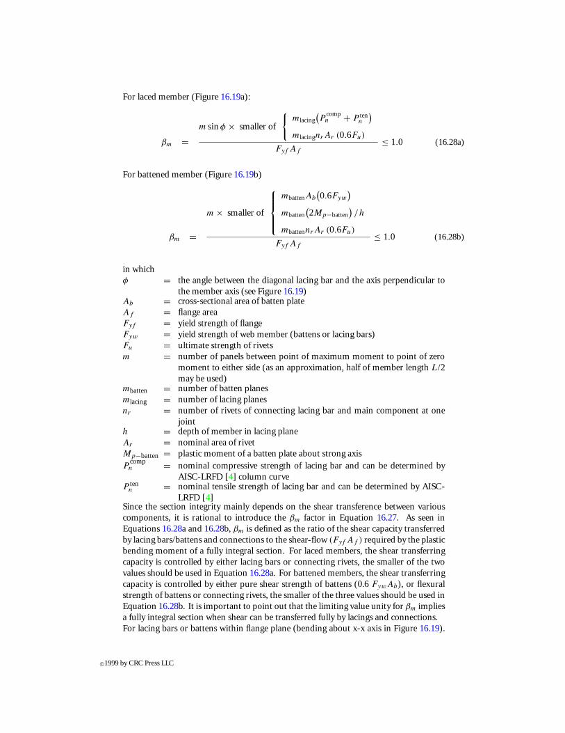
For laced member (Figure 16.19a):

βm =m sinφ × smaller of

{mlacing

(P

compn + P ten

n

)mlacingnrAr (0.6Fu)

Fyf Af

≤ 1.0 (16.28a)

For battened member (Figure 16.19b)

βm =

m × smaller of

mbattenAb

(0.6Fyw

)mbatten

(2Mp−batten

)/h

mbattennrAr (0.6Fu)

Fyf Af

≤ 1.0 (16.28b)

in whichφ = the angle between the diagonal lacing bar and the axis perpendicular to

the member axis (see Figure 16.19)Ab = cross-sectional area of batten plateAf = flange areaFyf = yield strength of flangeFyw = yield strength of web member (battens or lacing bars)Fu = ultimate strength of rivetsm = number of panels between point of maximum moment to point of zero

moment to either side (as an approximation, half of member length L/2may be used)

mbatten = number of batten planesmlacing = number of lacing planesnr = number of rivets of connecting lacing bar and main component at one

jointh = depth of member in lacing planeAr = nominal area of rivetMp−batten = plastic moment of a batten plate about strong axisP

compn = nominal compressive strength of lacing bar and can be determined by

AISC-LRFD [4] column curveP ten

n = nominal tensile strength of lacing bar and can be determined by AISC-LRFD [4]

Since the section integrity mainly depends on the shear transference between variouscomponents, it is rational to introduce the βm factor in Equation 16.27. As seen inEquations 16.28a and 16.28b, βm is defined as the ratio of the shear capacity transferredby lacing bars/battens and connections to the shear-flow (Fyf Af ) required by the plasticbending moment of a fully integral section. For laced members, the shear transferringcapacity is controlled by either lacing bars or connecting rivets, the smaller of the twovalues should be used in Equation 16.28a. For battened members, the shear transferringcapacity is controlled by either pure shear strength of battens (0.6 FywAb), or flexuralstrength of battens or connecting rivets, the smaller of the three values should be used inEquation 16.28b. It is important to point out that the limiting value unity for βm impliesa fully integral section when shear can be transferred fully by lacings and connections.For lacing bars or battens within flange plane (bending about x-x axis in Figure 16.19).


The contribution of lacing bars is assumed negligible and only the main components areconsidered.

Ix−x =∑

I(x−x)i +∑

Aiy2i (16.29)

3. Elastic section modulus

S = I

C(16.30)

whereS = elastic section modulus of a sectionC = distance from elastic neutral axis to extreme fiber

4. Plastic section modulusFor lacing bars or battens within flange plane (bending about x-x axis in Figure 16.19)

Zx−x =∑

y∗i A∗

i (16.31)

For lacing bars or battens within web plane (bending about y-y axis in Figure 16.19)

Zy−y = βm

∑x∗i A∗

i (16.32)

whereZ = plastic section modulus of a section about plastic neutral axisx∗i = distance between center of gravity of a section A∗

i and plastic neutral y-y axisy∗i = distance between center of gravity of a section A∗

i and plastic neutral x-x axisA∗

i = cross-section area above or below plastic neutral axis

It should be pointed out that the plastic neutral axis is generally different from the elasticneutral axis. The plastic neutral axis is defined by equal plastic compression and tensionforces for this section.

5. Torsional constantFor a box-shaped section

J = 4 (Aclose)2∑ bi

ti

(16.33)

For an open thin-walled section

J =∑ bit

3i

3(16.34)

whereAclose = area enclosed within mean dimension for a boxbi = length of a particular segment of the sectionti = average thickness of segment bi

For determination of torsional constant of a latticed member, it is proposed that the lacingbars or batten plates be replaced by reduced equivalent thin-walled plates defined as:


Aequiv = βtA∗equiv (16.35)

For laced member (Figure 16.19a)

A∗equiv = 3.12Ad sinφ cos2 φ (16.36a)


A∗equiv = 74.88

2ahIb

+ a2

If

(16.36b)

tequiv = Aequiv

h(16.37)

wherea = distance between two battens along member axisAequiv = cross-section area of a thin-walled plate equivalent to lacing bars considering

shear transferring capacityA∗

equiv = cross-section area of a thin-walled plate equivalent to lacing bars or battensassuming full section integrity

tequiv = thickness of equivalent thin-walled plateAd = cross-sectional area of all diagonal lacings in one panelIb = moment of inertia of a batten plateIf = moment of inertia of a side solid flange about the weak axisβt = reduction factor for torsion constant may be determined by the following

formula:

For laced member (Figure 16.19a)

βt =cosφ × smaller of

{P

compn + P ten

n

nrAr (0.6Fu)

0.6FywA∗equiv

≤ 1.0 (16.38a)


βt =smaller of

Ab

(0.6Fyw

)h/a

2Mp−batten/a

nrAr (0.6Fu) h/a

0.6FywA∗equiv

≤ 1.0 (16.38b)

The torsional integrity is from lacings and battens. A reduction factor βt , similar to thatused for the moment of inertia, is introduced to consider section integrity when the lacingis weaker than the solid plate side of the section. βt factor is defined as the ratio of theshear capacity transferredby lacingbars andconnections to the shear-flow (0.6FywA∗

equiv)

required by the equivalent thin-walled plate. It is seen that the limiting value of unity forβt implies a fully integral section when shear in the equivalent thin-walled plate can betransferred fully by lacings and connections.


Based on the equal lateral stiffness principle, an equivalent thin-walled plate for a lacingplane, Equation 16.36a and 16.36b can be obtained by considering E/G = 2.6 for steelmaterial and shape factor for shear n = 1.2 for a rectangular section.

6. Warping constantFor a box-shaped section

Cw ≈ 0 (16.39)

For an I-shaped section

Cw = If h2

2(16.40)

whereIf = moment of inertia of one solid flange about the weak axis (perpendicular to the

flange) of the cross-sectionh = distance between center of gravity of two flanges

16.A.2 Buckling Mode Interaction For Compression Built-up members

An important phenomenon of the behavior of these compressive built-up members is the interac-tion of buckling modes [9]; i.e., interaction between the individual (or local) component buckling(Figure 16.20a) and the global member buckling (Figure 16.20b). This section presents the practicalapproach proposed by Duan, Reno, and Uang [22] that may be used to determine the effects ofinteraction of buckling modes for capacity assessment of existing built-up members.

Buckling Mode Interaction Factor

To consider buckling mode interaction between the individual components and the globalmember, it is proposed that the usual effective length factor K of a built-up member be multipliedby a buckling mode interaction factor, γLG, that is,

KLG = γLGK (16.41)

whereK = usual effective length factor of a built-up memberKLG = effective length factor considering buckling model interaction

Limiting Effective Slenderness Ratios

For practical design, the following two limiting effective slenderness ratios are suggested forconsideration of buckling mode interaction:

Kaa/rf = 1.1√

E/F (16.42)

Kaa/rf = 0.75(KL/r) (16.43)

where (Kaa/rf ) is the largest effective slenderness ratio of individual components between connec-tors and (KL/r) is governing effective slenderness ratio of a built-up member.

The first limit Equation 16.42 is based on the argument that if an individual component is veryshort, the failure mode of the component would be material yielding (say 95% of the yield load), notmember buckling. This implies that no interaction of buckling modes occurs when an individualcomponent is very short.


FIGURE 16.20: Buckling modes of built-up members.

The second limit Equation 16.43 is set forth by the current design specifications. Both the AISC-LRFD [4] and AASHTO-LRFD [1] imply that when the effective slenderness ratio (Kaa/ri) ofeach individual component between the connectors does not exceed 75% of the governing effectiveslenderness ratio of the built-up member, no strength reduction due to interaction of buckling modesneeds to be considered. The study reported by Duan, Reno, and Uang [22] has justified that the ruleof (Kaa/ri) < 0.75(KL/r) is consistent with the theory.

Analytical Equation

The buckling mode interaction factor γLG is defined as:

γLG =√

PG

Pcr

=√

π2EI

(KL)2Pcr

(16.44)

wherePcr = elastic buckling load considering buckling mode interactionPG = elastic buckling load without considering buckling mode interactionL = unsupported member lengthI = moment of inertia of a built-up memberγLG can be computed by the following equation:

γLG =√√√√√√√√√

1 + α2

1 + α2

1+ (δo/a)2(Kaa/rf )2

2

[1− (Kaa/rf )2

(γLGKL/r)2

]3

(16.45)


where

(δo/a) = imperfection (out-of-straightness) parameter of individual component (see Figure 16.21)

α = separation as defined as:

α = h

2

√Af

If

= h

2rf(16.46)

in which

If = moment inertia of one side individual components (see Figure 16.21)

Af = cross-section area of one side individual components (see Figure 16.21)

h = depth of latticed member, distance between center of gravity of two flanges in lacing plane(see Figure 16.21)

r = radius of gyration of a built-in member

rf = radius of gyration of individual component

FIGURE 16.21: Typical cross-section and local components.

For widely separated built-up members with α ≥ 2, the buckling mode interaction factor γLG canbe accurately estimated by the following equation on the conservative side:

γLG =√√√√√1 + (δo/a)2(Kaa/rj )2

2[1 − (Kaa/rj )2

(γLGKL/r)2

]3(16.47)

Graphical Solution

Although γLG can be obtained by solving Equation 16.45, an iteration procedure must beused. For design purposes, solutions in chart forms are more desirable. Figures 16.22 to 16.24provide engineers with alternative graphic solutions for widely separated built-up members withα ≥ 2. In these figures, the out-of-straightness ratios (δo/a) considered are 1/500, 1/1000, and1/1500, and the effective slenderness ratios (KL/r) considered are 20, 40, 60, 100, and 140. In allthese figures, the top line represents KL/r = 20and the bottom line represents KL/r = 140.


FIGURE 16.22: Buckling mode interaction factor γLG for δ0/a = 1/500.


16.A.3 Acceptable Force D/C Ratios and Limiting Values

Since it is uneconomical and impossible to design bridges to withstand seismic forces elastically, thenon-linear inelastic responses of the bridges are expected. The performance-based criteria acceptscertain seismic damage in some other components so that the critical components and the bridges willbe kept essentially elastic and functional after the SEE and FEE. This section presents the concept ofacceptable force D/C ratios, limiting member slenderness parameters and limiting width-thicknessratios, as well as expected ductility.



FIGURE 16.25: Definition of force D/C ratios for combined loadings.

Definition of Force Demand/Capacity (D/C) Ratios

For members subjected to an individual load, force demand is defined as a factored individualforce, such as factored moment, shear, axial force, etc. which shall be obtained by the nonlineardynamic time history analysis – Level I specified in Section 16.6, and capacity is defined accordingto the provisions in Section 16.7.

For members subjected to combined loads, force D/C ratio is based on the force interaction.For example, for a member subjected to combined axial load and bending moment (Figure 16.25),force demand D is defined as the distance from the origin point O(0, 0) to the factored force pointd(Pu, Mu), and capacity C is defined as the distance from the origin point O(0, 0) to the pointc(P ∗, M∗) on the specified interaction surface or curve (failure surface or curve).


Ductility and Load-Deformation Curves

“Ductility” is usually defined as a nondimensional factor, i.e., ratio of ultimate deformation toyield deformation [20, 34]. It is normally expressed by two forms:

1. curvature ductility (µφ = φu/φy)

2. displacement ductility (µ1 = 1u/1y)

Representing section flexural behavior, curvature ductility is dependent on the section shape andmaterial properties. It is based on the moment-curvature curve. Indicating structural system ormember behavior, displacement ductility is related to both the structural configuration and its sectionbehavior. It is based on the load-displacement curve.

A typical load-deformation curve including both the ascending and descending branches is shownin Figure 16.26. The yield deformation (1y or φy) corresponds to a loading state beyond which thestructure starts to respond inelastically. The ultimate deformation (1u or φu) refers to the a loadingstate at which a structural system or a structural member can undergo without losing significantload-carrying capacity. It is proposed that the ultimate deformation (curvature or displacement) isdefined as the deformation corresponding to a load that drops a maximum of 20% from the peakload.

FIGURE 16.26: Load-deformation curves.

Force D/C Ratios and Ductility

The following discussion will give engineers a direct measure of seismic damage of structuralcomponents during an earthquake. Figure 16.27 shows a typical load-response curve for a singledegree of freedom system. Displacement ductility is:

µ1 = 1u

1y

(16.48)

A new term, Damage Index, is defined herein as the ratio of elastic displacement demand to ultimate


FIGURE 16.27: Response of a single degree of freedom of system.

displacement:

D1 = 1ed

1u

(16.49)

When damage index D1 < 1/µ1 (1ed < 1y), it implies that no damage occurs and the structureresponds elastically; 1/µ1 < D1 < 1.0 indicates certain damages occur and the structure respondsinelastically; D1 > 1.0, however, means that a structural system collapses.

Based on the equal displacement principle, the following relationship is obtained as:

Force Demand

Force Capacity= 1ed

1y

= µ1D1 (16.50)

It is seen from Equation 16.50 that the force D/C ratio is related to both the structural charactersin terms of ductility µ1 and the degree of damage in terms of damage index D1. Table 16.4 showsdetailed data for this relationship.

TABLE 16.4 Force D/C Ratio and Damage

IndexForce Damage Expected system displacementD/C index ductilityratio D1 µ1

1.0 No damage No requirement1.2 0.4 3.01.5 0.5 3.02.0 0.67 3.02.5 0.83 3.0

General Limiting Values

To ensure the important bridges have ductile load paths, general limiting slenderness parametersand width-thickness ratios are specified in Sections 16.8.3 and 16.8.4.

For steel members, λcr is the limiting member slenderness parameter for column elastic bucklingand is taken as 1.5 from AISC-LRFD [4] and λbr is the limiting member slenderness parameter for


beam elastic torsional buckling and is calculated by AISC-LRFD [4]. For a critical member, a morestrict requirement, 90% of those elastic buckling limits is proposed. Regardless of the force D/Cratios, all steel members must not exceed these limiting values. For existing steel members with D/Cratios less than one, this limit may be relaxed.

For concrete members, the general limiting parameter KL/r = 60 is proposed.

Acceptable Force D/C Ratios DCaccept

Acceptable force D/C ratios (DCaccept) depends on both the structural characteristics in terms ofductility µ1 and the degree of damage to the structure that can be accepted by practicing engineersin terms of damage index D1.

To ensure a steel member has enough inelastic deformation capacity during an earthquake, it isnecessary to limit both the member slenderness parameters and the section width-thickness ratioswithin the specified ranges so that the acceptable D/C ratios and the energy dissipation can beachieved.

Upper Bound Acceptable D/C Ratio DCp

1. For other members, the large acceptable force D/C ratios (DCp = 2 to 2.5) are proposedin Table 16.2. This implies that the damage index equals 0.67 ∼ 0.83 and more damagewill occur at other members and large member ductility will be expected. To achieve this,

• the limiting width-thickness ratio was taken as λp−Seismic from AISC-Seismic Pro-visions [5], which can provide flexural ductility 8 to 10.

• the limiting slendernessparameterswere takenasλbp forflexuralmomentdominantmembers from AISC-LRFD [4], which can provide flexural ductility 8 to 10.

2. For critical members, small acceptable force D/C ratios (DCp = 1.2 to 1.5) are proposedin Table 16.2, as the design purpose is to keep critical members essentially elastic andallow little damage (damage index equals to 0.4 ∼ 0.5). Thus, small member ductility isexpected. To achieve this,

• the limiting width-thickness ratio was taken as λp from AISC-LRFD [5], which canprovide flexural ductility at least 4.

• the limiting slendernessparameterswere takenasλbp forflexuralmomentdominantmembers from AISC-LRFD [4], which can provide flexural ductility at least 4.

3. For axial load dominant members, the limiting slenderness parameters were taken asλcp = 0.5, corresponding to 90% of the axial yield load by the AISC-LRFD [4] columncurve. This limit will provide the potential for axial load dominated members to developexpected inelastic deformation.

Lower Bound Acceptable D/C Ratio DCr

The lower bound acceptable force D/C ratio DCrc = 1 is proposed in Table 16.2. For DCaccept =1,it is unnecessary to enforce more strict limiting values for members and sections. Therefore, thelimiting slenderness parameters for elastic global buckling specified in Table 16.2 and the limitingwidth-thickness ratios specified in Table 16.3 for elastic local buckling are proposed.

Acceptable D/C Ratios Between Upper and Lower Bounds DCr < DCaccept < DCp

When acceptable force D/C ratios are between the upper and the lower bounds, DCr < DCaccept <

DCp , a linear interpolationas shown inFigure16.28 is proposed todetermine the limiting slenderness


parameters and width-thickness ratios. The following formulas can be used:

λpr =

[λp + (

λr − λp

) (DCp−DCaccept

DCp−DCr

)]for critical members[

λp−Seismic + (λr − λp−Seismic

) (DCp−DCaccept

DCp−DCr

)]for other members

(16.51)

FIGURE 16.28: Acceptable D/C ratios and limiting slenderness parameters and width-thicknessratios.

For axial load dominant members (Pu/Pn ≥ Mu/Mn)

λcpr =

λcp + (0.9λcr − λcp

) (DCp−DCaccept

DCp−DCr


λcp + (λcr − λcp

) (DCp−DCaccept

DCp−DCr

)for other members

(16.52)

For flexural moment dominant members (Mu/Mn > Pu/Pn)

λbpr =

λbp + (0.9λbr − λbp

) (DCp−DCaccept

DCp−DCr


λbp + (λbr − λbp

) (DCp−DCaccept

DCp−DCr

)for other members

(16.53)

where λr, λp, λp−Seismic are limiting width-thickness ratios specified by Table 16.3.

Limiting Width-Thickness Ratios

The basic limiting width-thickness ratios λr, λp, λp−Seismic specified in Table 16.3 are proposedfor important bridges.

16.A.4 Inelastic Analysis Considerations

This section presents concepts and formulas of reduced material and section properties and yieldsurface for steel members for possible use in inelastic analysis.


Stiffness Reduction

Concepts of stiffness reduction — tangent modulus — have been used to calculate inelasticeffective length factors by AISC-LRFD [4], and to account for both the effects of residual stresses andgeometrical imperfection by Liew [32].

To consider inelasticity of a material, the tangent modulus of the material Et may be used inanalysis. For practical application, stiffness reduction factor (SRF) = (Et/E) can be taken as theratio of the inelastic to elastic buckling load of the column:

SRF = Et

E≈ (Pcr )inelastic

(Pcr )elastic(16.54)

where (Pcr )inelastic and (Pcr )elastic can be calculated by AISC-LRFD [4] column equations:

(Pcr )inelastic = 0.658λ2c AsFy (16.55)

(Pcr )elastic =[

0.877

λ2c

]AsFy (16.56)

in which As is the gross section area of the member and λc is the slenderness parameter. By utilizingthe calculated axial compression load P , the tangent modulus Et can be obtained as:

Et ={

E for P/Py ≤ 0.39−3(P/Py) ln(P/Py) for P/Py > 0.39

(16.57)

Reduced Section Properties

In an initial structural analysis, the section properties based on a fully integral section of alatticed member may be used. If section forces obtained from this initial analysis are lower thanthe section strength controlled by the shear-flow transferring capacity, assumed fully integral sectionproperties used in the analysis are rational. Otherwise, section properties considering a partiallyintegral section, as discussed in Section 17.A.1, Iequiv and Jequiv , may be used in the further analysis.This concept is similar to “cracked section” analysis for reinforced concrete structures [13].

1. Moment of inertia — latticed members

(a) For lacing bars or battens within web plane (bending about y-y axis in Fig-ure 16.19)

The following assumptions are made:

• Moment-curvature curve (Figure 16.29) behaves bi-linearly until the section reachesits ultimate moment capacity.

• For moments less than Md = βm Mu, the moment at first stiffness degradation, thesection can be considered fully integral.

• For moments larger than Md and less than Mu, the ultimate moment capacity of thesection, the section is considered as a partially integral one; that is, bending stiffnessshould be based on a reduced moment of inertia defined by Equation 16.27.

An equivalent moment of inertia, Iequiv , based on the secant stiffness can be obtained as:

Iequiv = I ∗y−yIy−y

βmIy−y + (1 − βm)I ∗y−y

(16.58)


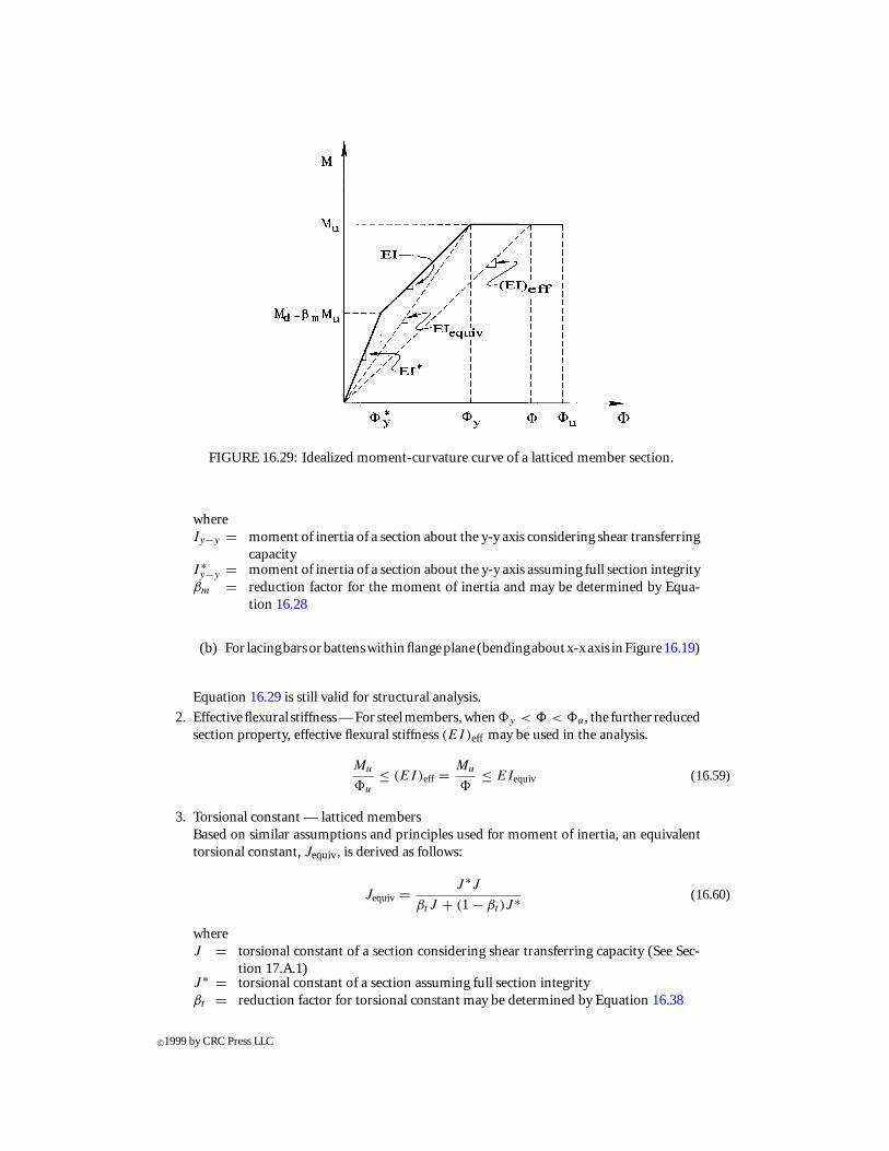
FIGURE 16.29: Idealized moment-curvature curve of a latticed member section.

whereIy−y = moment of inertia of a section about the y-y axis considering shear transferring

capacityI ∗y−y = moment of inertia of a section about the y-y axis assuming full section integrity

βm = reduction factor for the moment of inertia and may be determined by Equa-tion 16.28

(b) For lacingbarsorbattenswithinflangeplane (bendingaboutx-xaxis inFigure16.19)

Equation 16.29 is still valid for structural analysis.

2. Effectiveflexural stiffness—For steelmembers, when8y < 8 < 8u, the further reducedsection property, effective flexural stiffness (EI)eff may be used in the analysis.

Mu

8u

≤ (EI)eff = Mu

8≤ EIequiv (16.59)

3. Torsional constant — latticed membersBased on similar assumptions and principles used for moment of inertia, an equivalenttorsional constant, Jequiv , is derived as follows:

Jequiv = J ∗JβtJ + (1 − βt )J ∗ (16.60)

whereJ = torsional constant of a section considering shear transferring capacity (See Sec-

tion 17.A.1)J ∗ = torsional constant of a section assuming full section integrityβt = reduction factor for torsional constant may be determined by Equation 16.38


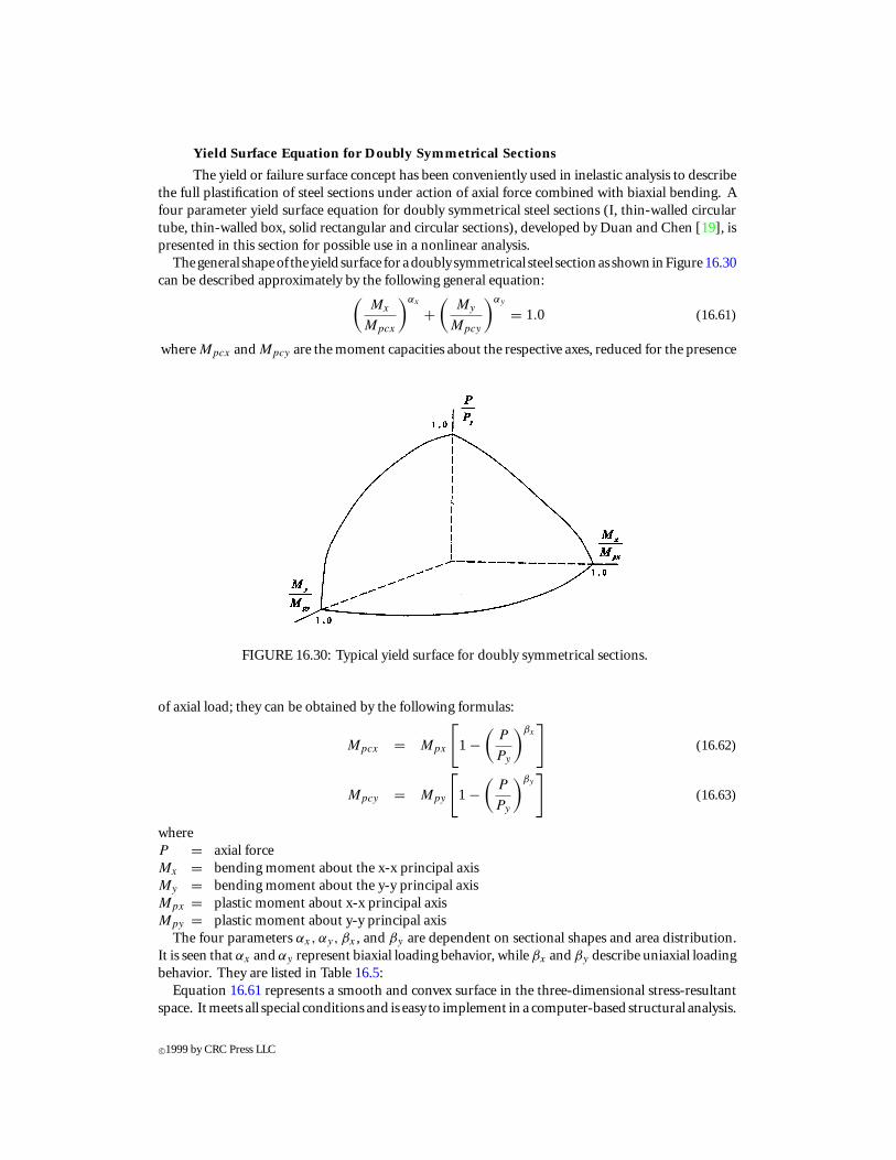
Yield Surface Equation for Doubly Symmetrical Sections

The yield or failure surface concept has been conveniently used in inelastic analysis to describethe full plastification of steel sections under action of axial force combined with biaxial bending. Afour parameter yield surface equation for doubly symmetrical steel sections (I, thin-walled circulartube, thin-walled box, solid rectangular and circular sections), developed by Duan and Chen [19], ispresented in this section for possible use in a nonlinear analysis.

Thegeneral shapeof theyield surface for adoubly symmetrical steel sectionas shown inFigure 16.30can be described approximately by the following general equation:(

Mx

Mpcx

)αx

+(

My

Mpcy

)αy

= 1.0 (16.61)

where Mpcx and Mpcy are the moment capacities about the respective axes, reduced for the presence

FIGURE 16.30: Typical yield surface for doubly symmetrical sections.

of axial load; they can be obtained by the following formulas:

Mpcx = Mpx

[1 −

(P

Py

)βx]

(16.62)

Mpcy = Mpy

[1 −

(P

Py

)βy]

(16.63)

whereP = axial forceMx = bending moment about the x-x principal axisMy = bending moment about the y-y principal axisMpx = plastic moment about x-x principal axisMpy = plastic moment about y-y principal axis

The four parameters αx, αy, βx , and βy are dependent on sectional shapes and area distribution.It is seen that αx and αy represent biaxial loading behavior, while βx and βy describe uniaxial loadingbehavior. They are listed in Table 16.5:

Equation 16.61 represents a smooth and convex surface in the three-dimensional stress-resultantspace. It meets all special conditions and is easy to implement in a computer-based structural analysis.


TABLE 16.5 Parameters for Doubly Symmetrical SectionsSection types αx αy βx βy

Solid rectangular 1.7 + 1.3 (P/Py) 1.7 + 1.3 (P/Py) 2.0 2.0Solid circular 2.0 2.0 2.1 2.1I-shape 2.0 1.2 + 2 (P/Py) 1.3 2 + 1.2 (Aw/Af )

Thin-walled box 1.7 + 1.5 (P/Py) 1.7 + 1.5 (P/Py) 2 − 0.5 B ≥ 1.3 2 − 0.5 B ≥ 1.3

Thin-walled circular 2.0 2.0 1.75 1.75

Note: B is the ratio of width-to-depth of the box section with respect to the bending axis.


performance-based seismic design criteria for bridgesfreeit.free.fr/structure engineering...

Documents