performance and reliability evaluation for dsrc vehicular

Performance and Reliability Evaluation for DSRC Vehicular Safety Communication

by

Xiaoyan Yin

Department of Electrical and Computer Engineering

Duke University

Date:_______________________

Approved:

___________________________

Kishor S. Trivedi, Supervisor

___________________________

Benjamin C. Lee

___________________________

Jeffrey H. Derby

___________________________

Loren W. Nolte

___________________________

Xiaomin Ma

Dissertation submitted in partial fulfillment of the requirements for the degree of

Doctor of Philosophy in the Department of Electrical and Computer Engineering

in the Graduate School of Duke University

2013

ABSTRACT

Performance and Reliability Evaluation for DSRC Vehicular Safety Communication

by

Xiaoyan Yin

Department of Electrical and Computer Engineering

Duke University

Date:_______________________

Approved:

___________________________

Kishor S. Trivedi, Supervisor

___________________________

Benjamin C. Lee

___________________________

Jeffrey H. Derby

___________________________

Loren W. Nolte

___________________________

Xiaomin Ma

An abstract of a dissertation submitted in partial fulfillment of the requirements for

the degree of Doctor of Philosophy in the Department of Electrical and Computer

Engineering in the Graduate School of Duke University

2013

Copyright by

Xiaoyan Yin

2013

iv

Abstract

Inter-Vehicle Communication (IVC) is a vital part of Intelligent Transportation

System (ITS), which has been extensively researched in recent years. Dedicated Short

Range Communication (DSRC) is being seriously considered by automotive industry

and government agencies as a promising wireless technology for enhancing

transportation safety and efficiency of road utilization. In the DSRC based vehicular ad

hoc networks (VANETs), the transportation safety is one of the most crucial features that

needs to be addressed. Safety applications usually demand direct vehicle-to-vehicle ad

hoc communication due to a highly dynamic network topology and strict delay

requirements. Such direct safety communication will involve a broadcast service because

safety information can be beneficial to all vehicles around a sender. Broadcasting safety

messages is one of the fundamental services in DSRC. In order to provide satisfactory

quality of services (QoS) for various safety applications, safety messages need to be

delivered both timely and reliably. To support the stringent delay and reliability

requirements of broadcasting safety messages, researchers have been seeking to test

proposed DSRC protocols and suggesting improvements. A major hurdle in the

development of VANET for safety-critical services is the lack of methods that enable one

to determine the effectiveness of VANET design mechanism for predictable QoS and

allow one to evaluate the tradeoff between network parameters. Computer simulations

v

are extensively used for this purpose. A few analytic models and experiments have been

developed to study the performance and reliability of IEEE 802.11p for safety-related

applications. In this thesis, we propose to develop detailed analytic models to capture

various safety message dissemination features such as channel contention, backoff

behavior, concurrent transmissions, hidden terminal problems, channel fading with path

loss, multi-channel operations, multi-hop dissemination in 1-Dimentional or 2-

Dimentional traffic scenarios. MAC-level and application-level performance metrics are

derived to evaluate the performance and reliability of message broadcasting, which

provide insights on network parameter settings. Extensive simulations in either Matlab

or NS2 are conducted to validate the accuracy of our proposed models.

vi

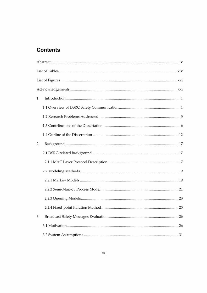
Contents

Abstract .................................................................................................................................... iv

List of Tables.......................................................................................................................... xiv

List of Figures ........................................................................................................................ xvi

Acknowledgements .............................................................................................................. xxi

1. Introduction ..................................................................................................................... 1

1.1 Overview of DSRC Safety Communication ............................................................... 1

1.2 Research Problems Addressed .................................................................................... 5

1.3 Contributions of the Dissertation ............................................................................... 6

1.4 Outline of the Dissertation ........................................................................................ 12

2. Background .................................................................................................................... 17

2.1 DSRC-related background ........................................................................................ 17

2.1.1 MAC Layer Protocol Description......................................................................... 17

2.2 Modeling Methods ..................................................................................................... 19

2.2.1 Markov Models ..................................................................................................... 19

2.2.2 Semi-Markov Process Model ................................................................................ 21

2.2.3 Queuing Models .................................................................................................... 23

2.2.4 Fixed-point Iteration Method ............................................................................... 25

3. Broadcast Safety Messages Evaluation ........................................................................ 26

3.1 Motivation .................................................................................................................. 26

3.2 System Assumptions ................................................................................................. 31

vii

3.3 Analytic Models ......................................................................................................... 33

3.3.1 SMP Model ............................................................................................................ 33

3.3.2 Service Time Computation ................................................................................... 37

3.3.3 Fixed-point Equation ............................................................................................ 42

3.3.4 Existence, Uniqueness and Convergence of Fixed-point Iteration .................... 46

3.3.4.1 Existence ......................................................................................................... 47

3.3.4.2 Uniqueness ..................................................................................................... 48

3.3.4.3 Convergence ................................................................................................... 49

3.4 Performance Indices .................................................................................................. 51

3.4.1 Mean Transmission Delay .................................................................................... 51

3.4.2 Packet Delivery Ratio ............................................................................................ 52

3.4.3 Packet Reception Ratio ......................................................................................... 54

3.5 Numerical and Simulation Results ........................................................................... 58

3.5.1 Numerical Vs. Simulation Results ....................................................................... 59

3.5.2 Comparison with Previous Models ..................................................................... 59

3.5.3 Impact Comparison between Concurrent Transmission and Hidden Terminals

......................................................................................................................................... 63

3.6 Conclusions and Future Work .................................................................................. 64

4. Periodic Beacon Messages Evaluation ......................................................................... 66

4.1 Motivation .................................................................................................................. 66

4.2 System Assumptions ................................................................................................. 72

4.3 Analytic Models ......................................................................................................... 73

viii

4.3.1 Overall Model ........................................................................................................ 73

4.3.2 SMP Model ............................................................................................................ 75

4.3.3 Service Time Computation ................................................................................... 80

4.3.4 Fixed-point Iteration ............................................................................................. 84

4.4 Performance Indices .................................................................................................. 88

4.4.1 MAC-level Performance Metrics ......................................................................... 88

4.4.1.1 Mean Transmission Delay ............................................................................. 88

4.4.1.2 Packet Delivery Ratio..................................................................................... 89

4.4.1.3 Packet Reception Ratio .................................................................................. 90

4.4.1.4 Normalized Channel Throughput ................................................................ 90

4.4.2 Application-level Performance Metrics ............................................................... 91

4.4.2.1 Node Reception Probability .......................................................................... 91

4.4.2.2 T-window Reliability ..................................................................................... 94

4.4.2.3 Application-level Delay ................................................................................. 95

4.4.2.4 Awareness Probability ................................................................................... 95

4.4.2.5 Average Number of Invisible Neighbors ..................................................... 96

4.5 Numerical Results ...................................................................................................... 96

4.5.1 Numerical Results for MAC-level Performance Metrics ................................... 97

4.5.1.1 Simulation Description .................................................................................. 97

4.5.1.2 Analytic Vs. Simulation Results .................................................................... 98

4.5.1.3 Compare with Previous Models ................................................................... 99

4.5.2 Analytic-Numerical Results for Application-level Performance Metrics ....... 102

ix

4.5.2.1 Analytic-numerical Results for Fixed Network Parameters ..................... 102

4.5.2.2 Analytic-numerical Results for Different Network Parameters ............... 105

4.6 VANET Applications Evaluation ........................................................................... 107

4.6.1 Application Requirements .................................................................................. 107

4.6.2 Case Studies for VANET Applications .............................................................. 108

4.6.2.1 Emergency Vehicle Warning ....................................................................... 108

4.6.2.2 Slow Vehicle Indication ............................................................................... 110

4.6.2.3 Rear-end Collision Warning ........................................................................ 111

4.7 Conclusions .............................................................................................................. 112

5. Multiple Types of Services Evaluation ....................................................................... 115

5.1 Motivation ................................................................................................................ 115

5.2 System Description and Assumptions ................................................................... 119

5.3 Analytic Models ....................................................................................................... 121

5.3.1 SMP Model for ACi Service ................................................................................ 122

5.3.2 Service Time Computation ................................................................................. 126

5.3.3 Fixed-point Iteration ........................................................................................... 132

5.4 MAC-level Performance Metrics ............................................................................ 135

5.4.1 Mean transmission delay .................................................................................... 135

5.4.2 Variance of the transmission delay .................................................................... 136

5.4.3 Packet Delivery Ratio (PDR) .............................................................................. 138

5.4.4 Packet Reception Ratio (PRR) ............................................................................ 140

5.5 Numerical Results .................................................................................................... 144

x

5.5.1 Influence of Packet Arrival Rate ........................................................................ 145

5.5.2 Influence of Packet Length ................................................................................. 147

5.5.3 Influence of Backoff Window Size ..................................................................... 148

5.5.4 Influence of Channel Sensing Time ................................................................... 150

5.5.5 Influence of Carrier Sensing Range ................................................................... 151

5.5.6 Hidden terminal Vs. Concurrent Transmission ................................................ 153

5.5.7 One Vs. Multiple Types of Services ................................................................... 154

5.5.8 Preemptive Priority ............................................................................................. 156

5.5.9 Strict Priority ....................................................................................................... 157

5.5.10 Variance of Transmission Delay ...................................................................... 158

5.6 GI/G/1 Queue Extension .......................................................................................... 159

5.6.1 SMP Model .......................................................................................................... 159



5.6.4 MAC-level Performance Metrics ....................................................................... 162

5.6.4.1 Mean Transmission Delay ........................................................................... 162

5.6.4.2 Variance of Transmission Delay ................................................................. 163

5.6.4.3 PDR ............................................................................................................... 165

5.6.4.4 PRR ................................................................................................................ 165

5.6.4.5 Numerical Results ........................................................................................ 165

5.7 A Case Study ............................................................................................................ 168

5.8 Conclusions .............................................................................................................. 171

xi

6. Multi-channel Operation Evaluation ......................................................................... 173

6.1 Motivation ................................................................................................................ 173

6.2 System Assumptions ............................................................................................... 176

6.3 Analytic Models ....................................................................................................... 177

6.3.1 Overall Method Description ............................................................................... 177

6.3.2 SMP Model .......................................................................................................... 178



6.4 Performance Metrics ................................................................................................ 185

6.4.1 MAC-level Performance Metrics ....................................................................... 185

6.4.1.1 Mean Transmission Delay ........................................................................... 185

6.4.1.2 Node Reception Probability (NRP) ............................................................. 185

6.4.1.3 Packet Reception Ratio (PRR) ..................................................................... 190

6.4.1.4 Packet Delivery Ratio (PDR) ....................................................................... 191

6.4.2 Application-level Performance Metrics ............................................................. 193

6.4.2.1 Application-level Delay ............................................................................... 193

6.4.2.2 T-window Reliability ................................................................................... 194

6.4.2.3 Awareness Probability ................................................................................. 194

6.4.2.4 Average Number of Invisible Neighbors ................................................... 194


6.5.1 Simulation Description ....................................................................................... 195

6.5.2 Numerical Results ............................................................................................... 195

xii

6.5.3 Impacts of Channel Switching and Channel Fading ........................................ 201

6.6 Conclusions .............................................................................................................. 203

7. Multi-hop Dissemination Evaluation ......................................................................... 205

7.1 Motivation ................................................................................................................ 205

7.2 System Description and Assumptions ................................................................... 208

7.3 Analytic Models ....................................................................................................... 210

7.3.1 Channel Fading Model ....................................................................................... 210

7.3.2 Rebroadcast Probability ...................................................................................... 212

7.3.2.1 Message-centric rebroadcast probability .................................................... 213

7.3.2.2 Receiver-centric rebroadcast probability .................................................... 214

7.3.3 Average Rebroadcast Distance........................................................................... 216

7.3.4 Average Number of Hops to Reach a Distance ................................................ 218

7.3.5 Average Rebroadcast Delay ............................................................................... 218

7.3.6 Average Delay to Reach a Distance ................................................................... 219

7.3.7 Metrics Related to Message Vanishing .............................................................. 220


7.5 Simplification of f(x,m) ............................................................................................ 225

7.5.1 m is a constant over [0, d] .................................................................................... 226

7.5.2 m is a piecewise function over [0, d] .................................................................. 228

7.6 Conclusions .............................................................................................................. 229

8. Two-Dimensional Network Evaluation ..................................................................... 230

8.1 Motivation ................................................................................................................ 230

xiii

8.2 System Assumptions ............................................................................................... 233

8.3 Analytic Models ....................................................................................................... 234

8.3.1 SMP Model .......................................................................................................... 234


8.3.3 Fixed-Point Iteration ........................................................................................... 239

8.4 Performance Metrics ................................................................................................ 241

8.4.1 Mean Transmission Delay .................................................................................. 241

8.4.2 Packet Delivery Probability ................................................................................ 242

8.4.3 Packet Reception Ratio ....................................................................................... 249


8.6 Conclusions .............................................................................................................. 256

9. Summary ...................................................................................................................... 258

Bibliography ......................................................................................................................... 263

Biography ............................................................................................................................. 274

xiv

List of Tables

Table 1.1: Summary of chapters ............................................................................................ 16

Table 3.1: DSRC communication parameter ........................................................................ 58

Table 3.2: Mean delay E[D] comparisons ............................................................................. 62

Table 3.3: PDR comparison ................................................................................................... 63

Table 3.4: PRR comparison .................................................................................................... 63

Table 4.1: Network parameter settings ............................................................................... 102

Table 5.1: DSRC parameters for EDCA mechanism .......................................................... 145

Table 5.2: Parameters for packet arrival rate influence evaluation .................................. 146

Table 5.3: Parameters for packet length influence evaluation .......................................... 148

Table 5.4: D1 for backoff window size ............................................................................... 149

Table 5.5: D2 for backoff window size ............................................................................... 149

Table 5.6: D1 for channel sensing time ............................................................................... 150

Table 5.7: D2 for channel sensing time ............................................................................... 150

Table 5.8: D1 for carrier sensing range ............................................................................... 152

Table 5.9: D2 for carrier sensing range ............................................................................... 152

Table 5.10: Parameters for reliability factors evaluation ................................................... 153

Table 5.11: Parameters for one type of service ................................................................... 154

Table 5.12: Parameters for multiple types of services using EDCA ................................. 154

Table 5.13: Parameters for preemptive priority ................................................................. 156

Table 5.14: Parameters for variance computation ............................................................. 158

xv

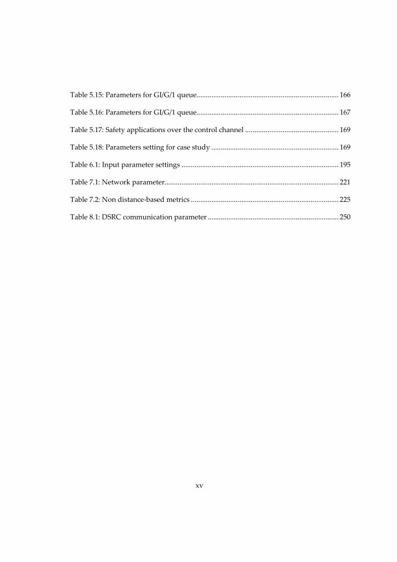
Table 5.15: Parameters for GI/G/1 queue............................................................................ 166

Table 5.16: Parameters for GI/G/1 queue............................................................................ 167

Table 5.17: Safety applications over the control channel .................................................. 169

Table 5.18: Parameters setting for case study .................................................................... 169

Table 6.1: Input parameter settings .................................................................................... 195

Table 7.1: Network parameter ............................................................................................. 221

Table 7.2: Non distance-based metrics ............................................................................... 225

Table 8.1: DSRC communication parameter ...................................................................... 250

xvi

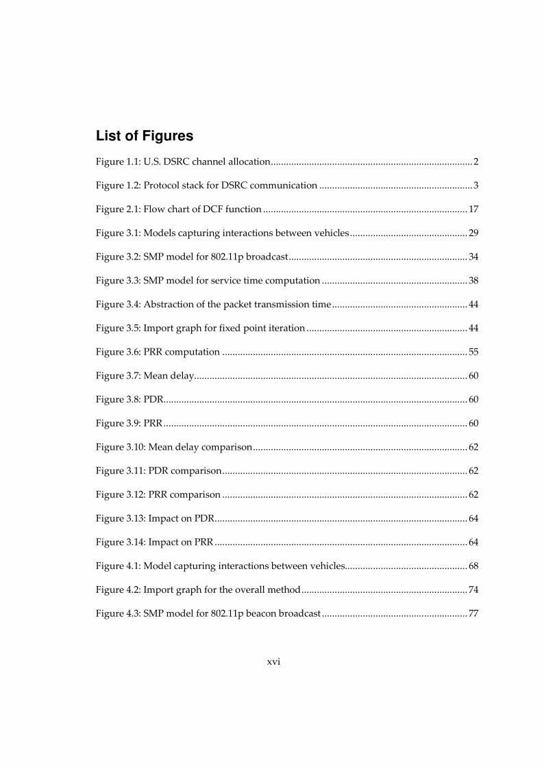
List of Figures

Figure 1.1: U.S. DSRC channel allocation ............................................................................... 2

Figure 1.2: Protocol stack for DSRC communication ............................................................ 3

Figure 2.1: Flow chart of DCF function ................................................................................ 17

Figure 3.1: Models capturing interactions between vehicles .............................................. 29

Figure 3.2: SMP model for 802.11p broadcast ...................................................................... 34

Figure 3.3: SMP model for service time computation ......................................................... 38

Figure 3.4: Abstraction of the packet transmission time ..................................................... 44

Figure 3.5: Import graph for fixed point iteration ............................................................... 44

Figure 3.6: PRR computation ................................................................................................ 55

Figure 3.7: Mean delay........................................................................................................... 60

Figure 3.8: PDR ....................................................................................................................... 60

Figure 3.9: PRR ....................................................................................................................... 60

Figure 3.10: Mean delay comparison .................................................................................... 62

Figure 3.11: PDR comparison ................................................................................................ 62

Figure 3.12: PRR comparison ................................................................................................ 62

Figure 3.13: Impact on PDR ................................................................................................... 64

Figure 3.14: Impact on PRR ................................................................................................... 64

Figure 4.1: Model capturing interactions between vehicles................................................ 68

Figure 4.2: Import graph for the overall method ................................................................. 74

Figure 4.3: SMP model for 802.11p beacon broadcast ......................................................... 77

xvii

Figure 4.4: SMP model with an absorbing state .................................................................. 81

Figure 4.5: Conceptual service time distribution ................................................................. 84

Figure 4.6: Channel sensing deference ................................................................................. 87

Figure 4.7: Node reception probability computation .......................................................... 92

Figure 4.8: Simulation flow chart .......................................................................................... 97

Figure 4.9: Mean transmission delay .................................................................................... 99

Figure 4.10: Packet delivery ratio .......................................................................................... 99

Figure 4.11: Packet reception ratio ........................................................................................ 99

Figure 4.12: Normalized channel throughput ..................................................................... 99

Figure 4.13: Comparison of mean delay ............................................................................. 102

Figure 4.14: Comparison of PDR ........................................................................................ 102

Figure 4.15: Comparison of PRR ......................................................................................... 102

Figure 4.16: Node reception probability (NRP) and awareness probability (PA) with

different packet requirement n ........................................................................................... 104

Figure 4.17: Application-level delay ................................................................................... 104

Figure 4.18: Average no. of invisible neighbors ................................................................ 104

Figure 4.19: Node reception probability (NRP) ................................................................. 106

Figure 4.20: Awareness probability PA(n=3) ..................................................................... 106

Figure 4.21: Application-layer delay .................................................................................. 106

Figure 4.22: Number of invisible neighbors ....................................................................... 106

Figure 4.23: Emergency vehicle warning application-level metrics with parameters

Rd=24, τ=0.2, PL=200 ............................................................................................................. 109

xviii

Figure 4.24: Slow vehicle indication application-level metrics with parameters Rd=24,

τ=0.2, PL=200 ........................................................................................................................ 110

Figure 4.25: Rear-end collision avoidance application layer metrics with parameters

Rd=24, τ=0.2, PL=200 ............................................................................................................. 112

Figure 5.1: SMP model for ACi message ............................................................................. 122

Figure 5.2: SMP model with absorbing state for service time computation .................... 126

Figure 5.3: Influence of packet arrival rate ......................................................................... 146

Figure 5.4: Influence of packet length................................................................................. 148

Figure 5.5: Influence of backoff window size .................................................................... 149

Figure 5.6: Influence of channel sensing time AIFS ........................................................... 151

Figure 5.7: Influence of carrier sensing range .................................................................... 152

Figure 5.8: Hidden terminal Vs. concurrent transmission ................................................ 154

Figure 5.9: One Vs. multiple types of services ................................................................... 155

Figure 5.10: Preemptive priority results ............................................................................. 156

Figure 5.11: Strict priority results........................................................................................ 157

Figure 5.12: Variance of the transmission delay ................................................................ 158

Figure 5.13: Output measures for GI/G/1 queue................................................................ 166

Figure 5.14: Output measures for M/G/1 queue ................................................................ 167

Figure 5.15: Applications with lower bound packet arrival rates .................................... 170

Figure 5.16: Applications with upper bound packet arrival rates .................................... 170

Figure 6.1: Import graph for the overall method ............................................................... 177

Figure 6.2: SMP model for a BSM transmission ................................................................. 178

Figure 6.3: A BSM transmission during CCH interval ...................................................... 182

xix

Figure 6.4: DIFS channel sensing during CCH interval .................................................... 184

Figure 6.5: MAC-level mean transmission delay ............................................................... 196

Figure 6.6: Packet transmission reliability ......................................................................... 197

Figure 6.7: Awareness probability with different packet requirements .......................... 199

Figure 6.8: Application-level delay ..................................................................................... 199

Figure 6.9: Average no. of invisible neighbors .................................................................. 200

Figure 6.10: Impacts of channel switching and channel fading on NRP ......................... 202

Figure 7.1: Message rebroadcast in a hop .......................................................................... 213

Figure 7.2: NRP and receiver-centric rebroadcast probability ......................................... 222

Figure 7.3: Number of hops to reach a distance ................................................................ 223

Figure 7.4: Average transmission delay ............................................................................. 223

Figure 7.5: Change order of double integral ...................................................................... 227

Figure 7.6: Fading parameter as a piecewise function ...................................................... 227

Figure 8.1: Hidden terminals problem for 1-D network ................................................... 231

Figure 8.2: Hidden terminals problem for 2-D network ................................................... 231

Figure 8.3: SMP model for IEEE 802.11 broadcast ............................................................. 235

Figure 8.4: Embedded DTMC of the SMP model for the service time ............................. 238

Figure 8.5: 2-D MANET model for performance analysis ................................................ 242

Figure 8.6: Illustration of S1 area calculation ...................................................................... 244

Figure 8.7: Illustration of S2 area calculation ...................................................................... 246

Figure 8.8: PRR with W0=15 ................................................................................................. 251

Figure 8.9: Mean transmission delay with W0=15 .............................................................. 252

xx

Figure 8.10: Impact of Nakagami fading on PRR of DSRC broadcast with network

parameters W0=15, λ=10 packets/s, Rd=24Mbps ................................................................. 252

Figure 8.11: PRR and PDP of DSRC broadcast with network parameters W0=15,

Rd=24Mbps, β=100/(πR2) ....................................................................................................... 253

Figure 8.12: PDP with network parameters λ=10 packets/s, W0=15, Rd=24Mbps,

β=100/(πR2) ............................................................................................................................ 253

Figure 8.13: Impact of Communication range on PRR of DSRC broadcast with network

parameters W0=15, λ=10 packets/s, Rd=24Mbps ................................................................. 254

xxi

Acknowledgements

I would like to express my deepest gratitude to my advisor, Dr. Kishor S. Trivedi,

for his guidance, patience, and encouragement during my research at Duke University.

Dr. Kishor S. Trivedi is a brilliant, extraordinary, and inspiring professor, who taught

me invaluable research skills, and helped me overcome many difficulties. He is always

there for me whenever I needed advice. The completion of this dissertation would be

impractical without his continuous academic and passionate support.

I will also forever be thankful to Prof. Xiaomin Ma, who gave me insightful

suggestions and invaluable comments on my work. During our research cooperation, he

has been extremely helpful in providing his scientific advice and knowledge through

many fruitful meetings and discussions. I sincerely treasure the collaboration

experiences with Prof. Ma.

I would like to thank my committee members during my research work, Dr. John

A. Board, Dr. Krishnendu Chakrabarty, Dr. Loren W. Nolte, and Dr. Matt Reynolds for

their kindness to serve on my committee and provide constructive suggestions to my

research.

I would like to thank the generous financial support for my research work from

National Science Foundation, Duke University Graduate School and Electrical and

Computer Engineering Department, General Motors and NEC Corporation.

xxii

I thank my colleagues at Duke University, Javier Alonso, Ermeson Andrade,

Rahul Ghosh, DongSeong Kim, Jae Shik Lim, Amita Devaraj, Fumio Machida, Arpan

Roy, Ruofan Xia, and Yang Zhao for their generous help and the wonderful working

environment that they created.

I would like to thank my farther Huasheng Yin, mother Zhiying Liu, elder sister

Dayan Yin and younger brother Jinzhong Yin for their unconditional love and

encouragement during the pursuit of my PhD degree. I am deeply grateful to my

husband Lei Zhang, who has been a true and great supporter during my good and bad

times. It is also a great pleasure and a wonderful life experience to have my beloved

daughter Jen Zhang born during this unique period of time.

1

1. Introduction

1.1 Overview of DSRC Safety Communication

Vehicle safety is an important issue for our society. Although severity

amelioration technologies such as air bags, seat belts, and automatic braking system

(ABS) have been applied for years to provide passive protection to vehicle occupants,

nearly 6.2 million police-reported motor vehicle crashes occur annually in the United

States (i.e., one every 5 seconds). On the average, a person is injured in a police-reported

motor vehicle crash every 12 seconds, and someone is killed every 12 minutes. The

related economic loss due to crashes is $230.6 billion annually. The development of

Intelligent Transportation System (ITS) [113] is to progress towards safe and smooth

driving without excessive delay. Vehicular ad hoc network (VANET) is one of the key

enabling technologies in ITS. Dedicated Short Range Communication (DSRC) radio

technology being standardized as IEEE 802.11p [1][112] is projected to support low-

latency wireless data communications between vehicles and from vehicles to roadside

units. Such a communication technology is being seriously considered by automotive

industry and government agencies, and the radio devices are expected to be installed in

future vehicles and work with sensors for enhancing transportation safety and efficiency

of road utilization.

Currently, DSRC is under active development in the United States, Europe,

Japan and other countries. Various safety and non-safety applications will be enabled

2

through information exchange using Vehicle-to-Vehicle (V2V) communication, and

Vehicle-to-Infrastructure (V2I) communication. Compared to non-safety applications

(e.g., toll collection, traffic indication, commercial services), safety applications (e.g.,

collision avoidance, emergency vehicle warning, slow vehicle indication) are more

critical to prevent collisions on the road and hence save thousands of lives. U.S.

Department of Transportation (DOT) has estimated that V2V safety communication

based on DSRC can assist drivers in preventing 76 percent of the crashes on the

roadway, thereby reducing fatalities and injuries that occur each year.

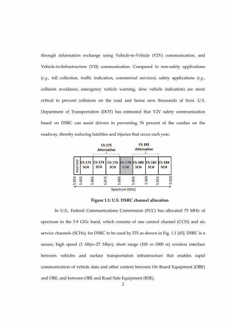
Figure 1.1: U.S. DSRC channel allocation

In U.S., Federal Communications Commission (FCC) has allocated 75 MHz of

spectrum in the 5.9 GHz band, which consists of one control channel (CCH) and six

service channels (SCHs), for DSRC to be used by ITS as shown in Fig. 1.1 [45]. DSRC is a

secure, high speed (3 Mbps~27 Mbps), short range (100 m~1000 m) wireless interface

between vehicles and surface transportation infrastructure that enables rapid

communication of vehicle data and other content between On Board Equipment (OBE)

and OBE, and between OBE and Road Side Equipment (RSE).

3

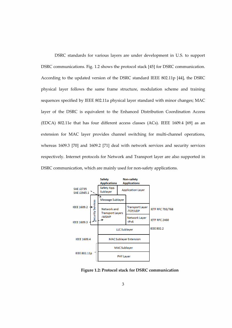
DSRC standards for various layers are under development in U.S. to support

DSRC communications. Fig. 1.2 shows the protocol stack [45] for DSRC communication.

According to the updated version of the DSRC standard IEEE 802.11p [44], the DSRC

physical layer follows the same frame structure, modulation scheme and training

sequences specified by IEEE 802.11a physical layer standard with minor changes; MAC

layer of the DSRC is equivalent to the Enhanced Distribution Coordination Access

(EDCA) 802.11e that has four different access classes (ACs). IEEE 1609.4 [69] as an

extension for MAC layer provides channel switching for multi-channel operations,

whereas 1609.3 [70] and 1609.2 [71] deal with network services and security services

respectively. Internet protocols for Network and Transport layer are also supported in

DSRC communication, which are mainly used for non-safety applications.

Figure 1.2: Protocol stack for DSRC communication

4

In the DSRC based vehicular ad hoc networks (VANETs), the transportation

safety is one of the most crucial features that need to be addressed. Safety applications

usually demand direct V2V ad hoc communication due to a highly dynamic network

topology and strict delay requirements. Such direct safety communication will involve a

broadcast service because safety information can be beneficial to all vehicles around a

sender. Broadcasting safety messages is one of the fundamental services in DSRC. The

safety messages can be categorized into two: basic safety message (BSM) and event-

driven safety message (ESM). The BSMs are periodically sent and also referred as

periodic beacon messages. The BSM contains information related to the status of vehicle

(e.g., position, velocity and direction) and is periodically broadcast by each vehicle to

announce other vehicles about their existence. Neighboring vehicles utilize such

messages to become aware of their surroundings out of sight and avoid potential

dangers (e.g., rear-end collision warning, slow vehicle indication, emergency vehicle

warning etc.) [58]. The ESMs are generated and broadcast by a vehicle to warn neighbors

around when an abnormal condition or an imminent danger is detected (e.g., road

hazard warning, traffic condition warning, signal violation warning etc.) [58]. In order to

provide satisfactory quality of services (QoS) for various safety applications, safety

messages need to be delivered in both reliably and timely manner.

5

1.2 Research Problems Addressed

To support the stringent delay and reliability requirements of broadcasting

safety messages, researchers have been seeking to test proposed DSRC protocols and

suggesting improvements. A major hurdle in the development of VANET for safety-

critical services is the lack of methods that enable one to determine the effectiveness of

VANET design mechanism for predictable QoS and allow one to evaluate the tradeoff

between network parameters. Hence, we aim to evaluate important performance and

reliability metrics under various traffic scenarios to assess the effectiveness of message

dissemination schemes for safety applications.

Several types of methods have been utilized in the literature to analyze the

performance and reliability for safety communication. Computer simulations are

extensively used, which usually take long time to collect sufficient data for accurate

performance analysis. Several real world experiments are also conducted to capture

more practical network dynamics. However, due to the high equipment cost, the

experimental testbed usually only consists of a very few vehicles. Even though some

techniques are used to create a large scale virtual communication network using a small

number of vehicles, the resulting virtual network is still only capable of capturing sparse

network scenarios. Analytic modeling is a more attractive alternative due to lower cost

of solving the model while covering a large network parameter space. However, there

are very few accurate analytic models developed for safety applications evaluation. Our

6

main goal for this dissertation is to propose comprehensive and high fidelity analytic

models for the performance and reliability analysis under various safety communication

scenarios. The accuracy and efficiency of the analytic models are validated through

extensive simulations.

1.3 Contributions of the Dissertation

In this dissertation, the following contributions are made:

(1) Developed comprehensive and high fidelity analytic models. In V2V safety

communications, vehicles on the road compete for the channel resource to transmit

their own safety messages. To reduce the complexity for developing and solving

monolithic models, we utilize the model decomposition technique and propose

interacting stochastic models based on the semi-Markov process (SMP) to capture

vehicles’ channel contention and backoff behavior. Due to the interactions between

vehicles, fixed-point iteration is used to obtain converged solutions, based on which

important performance and reliability metrics are further derived.

(2) Evaluated different types of safety messages. As mentioned earlier, the safety

messages can be categorized into two: basic safety message (BSM) and event-driven

safety message (ESM). A simplified SMP model is first developed for the ESM

evaluation, and a more precise SMP model is developed for the BSM evaluation. The

analytic-numerical results for these two approaches are also compared in Chapter 5.

The obtained results show that the performance and reliability metrics for BSM and

7

ESM are similar when their average message generation intervals are the same. In

addition, we conclude that the simplified SMP model for ESM evaluation with

Poisson message arrivals can be used to approximate the BSM evaluation with

periodic message arrivals. Many papers [6][8][41][52][62][117] have used Poisson

arrival process to approximate BSM arrival process without any proof.

(3) Evaluated multiple services over a single channel. The control channel (CCH) is the

default channel for V2V safety communication. If different types of safety messages

need to be transmitted to support multiple safety services, it is possible that the

control channel will be shared. Enhance distributed channel access (EDCA) is the

access mechanism specified in IEEE 802.11p protocol to support multiple types of

services with priorities. Therefore, analytic models are proposed for the performance

and reliability analysis of three types of vehicular safety-related services using

EDCA mechanism in the DSRC system on highways. Several important observations

are drawn. The results show that EDCA mechanism, which utilizes different channel

sensing time and backoff counters for different services, can only provide service

differentiation in terms of transmission delay, but cannot help improve the reliability

for higher priority services. Another important conclusion is that higher priority

service should choose shorter packet length, higher date rate and larger carrier

sensing range to ensure high packet transmission reliability.

8

(4) Evaluated multi-channel operations for the BSM. The control channel (CCH) is

dedicated to support safety communications, and BSM is most likely to be

transmitted via CCH. The SCH channel 172 in Fig. 1.1 is reserved probably for

critical V2V safety communications, and hence the ESM (which is sent in presence of

an emergency event and hence is more critical than BSM) can be transmitted on this

channel to avoid the channel contention with the more frequently generated BSMs.

In addition, other SCHs in Fig. 1.1 are most likely to be used for non-safety

applications. At the early stage of the DSRC deployment, a vehicle may only have a

single-radio device installed due to the cost constraints. To support both safety and

non-safety applications, this single-radio device can switch between different

channels, one channel at a time. IEEE 1609.4 [69] is an extension for MAC layer to

provide channel switching mechanism for multi-channel operations. Analytic

models are developed to evaluate the impact of such multi-channel operations on

the performance and reliability of BSMs transmitted via the CCH. The results show

that channel switching mechanism can greatly degrade the performance and

reliability of the BSM transmission.

(5) Evaluated multi-hop transmissions for the ESM. To ensure high reliability for

ESMs, which are more critical than BSMs, a channel (probably channel 172) may be

reserved specifically for ESM broadcasting. In addition, some event-driven safety

applications (e.g., post-crash notification, road hazard warning) may be required to

9

cover longer distances than the one-hop communication range. Therefore, multi-hop

ESM dissemination is necessary in such scenarios. A robust relay selection strategy

utilizing distance-based timers is proposed in this dissertation and an accurate

analytic model is proposed to evaluate multi-hop propagation of ESMs. Important

conclusions are drawn to provide deeper insight into the ESM transmission behavior

from different angles.

(6) Evaluated 2-Dimensional traffic scenarios. Most analytic models proposed in the

literature concentrate on 1-Dimensional (1-D) highway traffic to simplify the model.

Unfortunately, very few of network scenarios in real applications can be abstracted

as 1-D models. Therefore, in this dissertation, we first developed an analytic model

on the performance and reliability evaluation of 2-Dimensional (2-D) traffic at open

field to capture more realistic message transmission behaviors.

(7) Incorporated various factors for the performance and reliability metrics

derivation. In this dissertation, we considered various important factors that can

influence the message transmission including channel contention, backoff behavior,

concurrent transmissions, hidden terminals problems and channel fading with path

loss. The degree of impact of concurrent transmission, hidden terminals problem

and channel fading with path loss is also assessed. The results presented in Section

3.5.3, Section 5.5.6 and Section 6.5.3 show that concurrent transmission has very

10

minor impact, whereas hidden terminals problem and channel fading with path loss

have significant impact on the performance and reliability.

(8) Conducted simulations for cross validation purposes. We conducted extensive

simulations in either Matlab or NS2 for comparison purposes in each Chapter. The

good match between analytic-numerical results and simulation results under a large

range of network parameters validate the accuracy of our proposed models. In

addition, the time consumed to solve analytic models and for simulations is

compared, which shows that the analytic models are much more efficient than

simulations.

Our contribution can also be summarized from different aspects according to the interest

of people from various areas:

(1) Provide valuable insights for protocol development. First, we proposed an efficient

and accurate approach to easily evaluate whether the given network parameter can

satisfy the QoS and highlight how to tune the parameters in order to meet the QoS.

In addition, EDCA protocol is proven in this dissertation that it does not support

service differentiation regarding to broadcast reliability. Such observation may form

the background to support other effective protocols development for service

prioritization. Moreover, even though IEEE 802.11p is the standardized protocol

analyzed in this dissertation, our proposed models are based on characterizing the

operation flow for the DCF function, which forms the basic medium access

11

mechanism in many other protocols. Therefore, our models can be easily extended

to analyze other protocols.

(2) Provide more effective approach than simulation and experiment based methods.

To evaluate the effectiveness of our proposed analytical models, we conducted

simulations in every chapter for comparison purposes. Our models can be easily

solved within a few seconds or minutes, while simulations usually take up to several

hours. Hence, our models are much more efficient than simulation methods and can

deliver valuable results much faster for the development of DSRC safety

communication. Furthermore, most experiments are limited to a few vehicles due to

extremely high cost of purchasing vehicles, which results in the insufficiency for

capturing realistic and important factors that influence the safety communication,

such as hidden terminal problem. Therefore, the advantage of our model is that it

effectively considers various factors and can be easily extended to incorporate more

factors of interest without any resource limit.

(3) Provide more accurate approach than other analytic models. Even though there are

many analytic models proposed in the literature to analyze the performance and

reliability of safety communication, most of them are based on Bianchi’s discrete-

time Markov chain (DTMC) model [27]. The system’s continuous time behavior for

channel sensing and deferring in message transmission are completely ignored,

which results in inaccuracy. Our model considers more accurate message

12

transmission behavior in MAC layer by using semi-Markov Process (SMP) model

without discretizing the time. The comparison of our model with several DTMC

based analytic models presented in many chapters verifies that our model is more

accurate than prevalent DTMC models. In addition, most analytic models only

consider MAC-level performance metrics, whereas our model also considers

application-level metrics to better fulfill the safety application’s QoS requirement.

Moreover, several important factors such as distance-based channel fading, hidden

terminal problem and channel switching mechanism are not evaluated in vast

analytic approaches, while we constructed much more accurate and practical model

by taking into account of those essential factors.

1.4 Outline of the Dissertation

This dissertation is organized as follows:

Chapter 2 describes the background on DSRC-related topics and stochastic

modeling. Since the MAC layer channel access for safety communication follows

distributed coordination function (DCF) for one type of safety message according to

IEEE 802.11 protocol, the detailed DCF access control technique is first described. We

also introduce the related analytic modeling methods used throughout this dissertation.

Chapter 3 presents a general analytic model to evaluate the performance of

safety message broadcasting, which is suitable for ESMs. Poisson message arrival is

assumed for event-driven message generation. Infinite MAC-layer queue for each

13

vehicle is assumed since the ESMs are too critical to be dropped. Hence, the generation

and service of ESMs in each vehicle is modeled by a generalized M/G/1 queue. The

overall model is a set of interacting M/G/1 queues, one queue for each vehicle. To

produce a simplified yet high fidelity analytic model, we decompose the overall model

and use semi-Markov process (SMP) model to capture shared channel medium’s

behavior from a single vehicle’s perspective. Due to the interactions between vehicles,

fixed-point iteration is utilized to obtain converged solutions. Important MAC-level

performance and reliability metrics are subsequently derived. Simulations in Matlab are

developed to validate the accuracy and efficiency of the proposed analytic model.

Chapter 4 describes a more accurate analytic model to capture the BSM

broadcasting in a channel (probably the control channel), where associated features such

as periodic message generation, out-dated message replacement and no queuing in

MAC-layer are incorporated. Such a model for BSMs is compared with the model

presented in Chapter 3 for ESMs. The results prove that the simplified analytic model for

ESMs can be used to approximately evaluate the BSMs transmission. Besides MAC-level

performance and reliability metrics, application-level metrics are also evaluated.

Simulations in Matlab are conducted for the comparison purpose.

Since the control channel is the default channel for V2V safety communication,

multiple types of safety messages (including the ESM and BSM) can be transmitted

together in the control channel (CCH). Therefore, in Chapter 5, multiple types of services

14

transmissions over a single channel (e.g., control channel) are evaluated based on the

extension of the analytic model developed in Chapter 3. The EDCA mechanism specified

in the IEEE 802.11p protocol is shown to be ineffective to guarantee priorities for

different services. Important conclusions are also drawn to tune network parameters in

order to improve the performance and reliability for high priority services. Simulations

are performed in Matlab.

The U.S. FCC has allocated seven 10 MHz channels for DSRC: one control

channel (CCH) and six service channels (SCHs). At the early stage of DSRC deployment,

a vehicle may have only a single-radio DSRC device installed. To support concurrent

applications on different channels, such a single-radio device can switch between

different channels, one channel at a time, to access safety messages (e.g., BSMs) on the

CCH and other services on the SCHs. Therefore, the IEEE 1609.4 multi-channel

operation is considered in Chapter 6 to evaluate the performance and reliability of the

BSMs transmission on the CCH. The impacts of various factors such as concurrent

transmission, hidden terminals problem, channel fading with path loss and channel

switching mechanism are evaluated. Simulations are developed in NS2 to validate the

accuracy and efficiency of the proposed analytic model.

Among the six service channels, the Channel 172 may be reserved for life critical

safety applications with no time division [45]. This implied that a vehicle interested in

both safety and non-safety applications requires two DSRC radios: one tuned to Channel

15

172 all the time, and the other participates in IEEE 1609.4 channel switching [45]. Since

ESMs are life-critical messages, they are most likely to be transmitted on Channel 172. In

addition, since some event-driven safety applications (e.g., post-crash notification, road

hazard warning) may require longer transmission distance than the one-hop

communication range, multi-hop dissemination of ESMs is necessary. Hence, we

introduce an accurate analytic model in Chapter 7 to evaluate multi-hop propagation of

ESMs. Extensive Matlab simulations are performed. Important conclusions are obtained

to provide deeper understandings of the performance and reliability of the ESMs

transmission behavior.

The analytic models developed in Chapter 3-7 are all concentrated on 1-D

highway traffic to simplify the model. Until now, there is no analytic model on 2-D

evaluation. Nevertheless, very few of network scenarios in real applications can be

abstracted as 1-D traffic. Therefore, in Chapter 8, we first introduce an analytic model on

the performance and reliability evaluation of 2-D traffic at open field (i.e., battle field) to

capture more realistic message transmission behaviors. Simulations in NS2 are carried

out and the numerical results are compared with the analytic-numerical results under a

large range of network parameter settings.

Chapter 9 summarizes this dissertation and describes future research work on

this topic.

Table 1.1 summarizes and compares the work presented in each chapter.

16

Table 1.1: Summary of chapters

Chapter Message

Type

Multiple

Service?

Channel

Switch?

Multi-

hop? 2-D?

Fixed-

point? Simulation

3 BSM, ESM No No No No Yes Matlab, NS2

4 BSM No No No No Yes Matlab

5 BSM, ESM Yes No No No Yes Matlab

6 BSM No Yes No No Yes NS2

7 ESM No No Yes No No Matlab

8 BSM, ESM No No No Yes Yes NS2

17

2. Background

In this chapter, we briefly introduce the background on DSRC-related topics

(including DCF access mechanism) and stochastic modeling methods (including Markov

models, semi-Markov models and queuing models) used in this dissertation.

2.1 DSRC-related background

This section presents essential background of DSRC for analytic modeling of

safety communication in VANETs.

2.1.1 MAC Layer Protocol Description

Figure 2.1: Flow chart of DCF function

To model and assess the performance of safety message broadcasting, MAC layer

behavior specified by IEEE 802.11p has to be accurately evaluated. Hence, we briefly

describe the MAC layer channel access for safety message broadcasting in this section.

From [44], we know that the DSRC adopts IEEE 802.11 MAC layer specification

based on the carrier sense multiple access with collision avoidance (CSMA/CA) with

minor modifications. In the 802.11 MAC layer protocol [11], distributed coordination

function (DCF) is the primary medium access control technique for broadcast services.

18

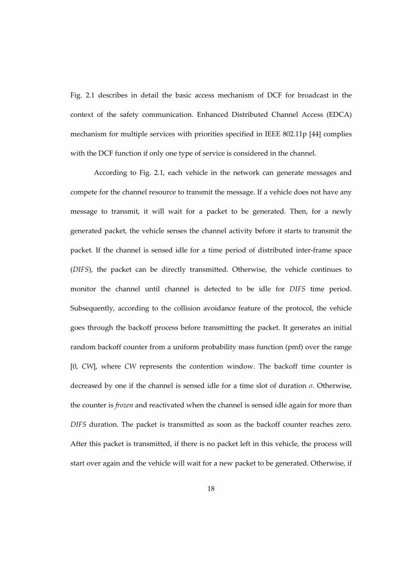
Fig. 2.1 describes in detail the basic access mechanism of DCF for broadcast in the

context of the safety communication. Enhanced Distributed Channel Access (EDCA)

mechanism for multiple services with priorities specified in IEEE 802.11p [44] complies

with the DCF function if only one type of service is considered in the channel.

According to Fig. 2.1, each vehicle in the network can generate messages and

compete for the channel resource to transmit the message. If a vehicle does not have any

message to transmit, it will wait for a packet to be generated. Then, for a newly

generated packet, the vehicle senses the channel activity before it starts to transmit the

packet. If the channel is sensed idle for a time period of distributed inter-frame space

(DIFS), the packet can be directly transmitted. Otherwise, the vehicle continues to

monitor the channel until channel is detected to be idle for DIFS time period.

Subsequently, according to the collision avoidance feature of the protocol, the vehicle

goes through the backoff process before transmitting the packet. It generates an initial

random backoff counter from a uniform probability mass function (pmf) over the range

[0, CW], where CW represents the contention window. The backoff time counter is

decreased by one if the channel is sensed idle for a time slot of duration σ. Otherwise,

the counter is frozen and reactivated when the channel is sensed idle again for more than

DIFS duration. The packet is transmitted as soon as the backoff counter reaches zero.

After this packet is transmitted, if there is no packet left in this vehicle, the process will

start over again and the vehicle will wait for a new packet to be generated. Otherwise, if

19

there are packets left, the vehicle repeats the procedure starting with sensing the channel

for DIFS duration and goes through the backoff procedure before transmitting the next

packet. According to the protocol, a vehicle must go through the backoff process

between two consecutive packet transmissions even if the channel is sensed idle for the

duration of DIFS time for the second packet.

2.2 Modeling Methods

To evaluate the performance and reliability of safety communication in VANETs,

state-space stochastic models are used in this dissertation to characterize the safety

message broadcasting behavior. Compared to non-state-space models, state-space

models can capture more complex dependencies in the system under consideration. This

section introduces some commonly used state-space models including Markov models

and semi-Markov models.

2.2.1 Markov Models

The stochastic process for Markov models is whose dynamic behavior for future

development depends only on the current state and not on how the process arrived in

that state, which is well known as Markov property. The formal definition for Markov

process is:

Definition: A stochastic process {X(t)|t ≥ 0} is a Markov chain if for any t0 < t1 < … < tn <

t, the conditional probability mass function (pmf) of X(t) satisfies:

20

( ) ( )1 1 0 0( ) | ( ) , ( ) ,..., ( ) ( ) | ( )n n n n n nP X t x X t x X t x X t x P X t x X t x− −= = = = = = = (2.1)

If the state space I is discrete as above, the Markov process is known as a Markov

chain. If the parameter space T is also discrete, then we have a discrete-time Markov

chain (DTMC). If the parameter space T is continuous, then we have a continuous-time

Markov chain (CTMC). The Markov chain {X(t)|t ≥ 0} is said to be (time-) homogeneous

if the state transition probability depends only on the difference of the two time epochs

that we are considering. Otherwise, the Markov chain is a non-homogeneous Markov

chain. Henceforth, we only consider the homogeneous case.

The transient behavior of a CTMC satisfies the Chapman-Kolmogorov equation

in matrix form as follows:

( )( )

d tt Q

dt=

ππ

(2.2)

where π(t) = [π1(t), π2(t), …, πn(t)] is the state probability vector, and n is the number of

states in the CTMC. Q = [qij]nxn is the infinitesimal generator matrix, where qij (i ≠ j) is the

transition rate from state i to state j, and qii = - ∑i≠j qij. In steady-state, Eq. (2.2) becomes:

0Q =π (2.3)

For a DTMC, the state probability vector after n-step transition is given by:

( ) (0) nn P= ⋅p p (2.4)

21

where p(0) = [p1(0), p2(0), …, pn(0)] is the initial state probability vector, and P = [pij]nxn is

the one-step transition probability matrix (pij is the transition probability from state i to

state j). In steady-state, denote lim ( )n n→∞=v p , then Eq. (2.4) becomes:

P= ⋅v v (2.5)

2.2.2 Semi-Markov Process Model

Semi-Markov process (SMP) model is a generalization of both continuous and

discrete time Markov chains which permit arbitrary sojourn time distribution function,

possibly depending on both the current state and the state to be visited next [116]. For a

better understanding, let us consider a stochastic process as follows [115]. First construct

a k-state discrete-time Markov chain (DTMC) with state transition probability matrix P =

[pij]; next construct a process in continuous time by marking the time spent in a

transition from state i to state j have a distribution function Fij(t) such that times are

mutually independent; at the end of the interval, we have a point event of type j. Such a

stochastic process is called semi-Markov process, which is a generalization of both

continuous and discrete time Markov processes with countable state spaces.

A descriptive definition of SMP [115] is that it is a stochastic process which

moves from one state to another state among a countable number of states with the

successive states visited forming a discrete-time Markov chain, and that the process

stays in a given state for a random amount of time, the distribution function of which

22

depends on this state as well as the one to be visited next but does not depend on which

states the system had been in before it got there.

A formal definition of SMP [116] is described as follows. A SMP is the process

Y={Yt; t≥0} defined by:

( ) 1,t N t n n n

Y X X if S t S += = ≤ < (2.6)

for t≥0, where N(t) is the counting process. From the SMP definition, it should be

observed that the process only changes state (possibly back to the same state) at the

Markov regeneration epochs Sn. To analyze the steady-state behavior or to calculate

some expected values of a SMP model, there exists a method called the two-stage

method. It describes an SMP model using the matrix P and the vector H(t), where P =

[pij] is the one-step transition probability matrix for the embedded Markov chain (EMC)

of the SMP model, and H(t)=[Hi(t)] with i=1,…,n, is the sojourn time distribution in state

i. Such a method considers SMP transitions as taking place in two stages:

1) In the first stage, the system stays in state i for some amount of time, the mean

sojourn time in state i is:

( )0

1 ( )i ih H t dt∞

= −∫ (2.7)

2) In the second stage, the system moves to state j with probability pij.

When this two-stage method is applied to the steady-state analysis of SMP model, we

first calculate the steady-state probability vector of the EMC using Eq. (2.5). Given the

23

mean sojourn time vector h=[h1, h2,…, hn], the steady-state probability vector π=[π1, π2,…,

πn] of the SMP can be written as:

0

i ii n

k k

k

v h

v h

π

=

=

∑

(2.8)

which is the ratio between the average time spent in state i (vihi) over the total average

time spent (∑kvkhk) over all states.

2.2.3 Queuing Models

A queuing system consists of one or more stations (servers) that provide services

to arriving customers (jobs). Customers who arrive to find all servers busy generally join

one or more queues (waiting lines) in front of the servers. The queuing system can be

characterized by three important components: arrival process, service process, and the

number of servers. Assume that successive inter-arrival times Y1, Y2, …, between jobs are

independent identically distributed random variables having a distribution FY. Similarly,

the service times S1, S2, …, are assumed to be independent identically distributed

random variables having a distribution FS. Let m denote the number of servers in the

system. Therefore, we can use the notation FY/ FS/m to describe the queuing system. The

following symbols are used to denote the specific types of inter-arrival times and service

time distributions [9]:

• M: (for memoryless) for the exponential distribution

• D: for a deterministic or constant inter-arrival or service time

24

• Ek: for a k-stage Erlang distribution

• Hk: for a k-stage hyperexponential distribution

• G: for a general distribution

• GI: for general independent inter-arrival times

Based on the above convention, we can easily interpret the queuing system. The most

frequent example of a queuing system is M/M/1 queue, which stands for a single-server

queue with exponentially distributed inter-arrival times and exponentially distributed

service time. In this dissertation, M/G/1 queue and GI/G/1 queue notions are used. M/G/1

queue represents a single-server queue with exponentially distributed inter-arrival times

and an arbitrary service time distribution, and GI/G/1 queue represents a single-server

queue with general independent inter-arrival times and an arbitrary service time

distribution. If a queuing system has limited buffer space so that at most n jobs can be in

the system, such a system can be denoted as FY/ FS/m/n using this Kendall notation.

Therefore, D/G/1/1 queue system presented in Section 4.1 denote a single-server queue

with deterministic inter-arrival times distribution, general service times distribution,

and the number of jobs in the system is at most 1. Besides the nature of the inter-arrival

time and service time distribution, queue scheduling discipline that describes how the

server is to be allocated to the jobs waiting for service also needs to be specified. In this

dissertation, two scheduling disciplines are used: First Come First Served (FCFS) and

Last Come First Served (LCFS).

25

2.2.4 Fixed-point Iteration Method

In numerical analysis, fixed-point iteration is a method used to compute fixed

points of iterated functions. More specifically, a solution to the equation f(x)=x is referred

to as a fixed point of the function f. Geometrically, the fixed points of a function f(x) are

the point(s) of intersection of the curve y=f(x) and the line y=x. Given a point x0 in the

domain of f, successive substitution xn+1 = f(xn), n=0,1,2,… is commonly used to determine

the fixed point. The sequence x0, x1, x2, …, is expected to converge to a point x. The

proofs for the existence, uniqueness and convergence of the fixed-point iteration process

are provided in Chapter 3.

26

3. Broadcast Safety Messages Evaluation

3.1 Motivation

In the DSRC based vehicular ad hoc networks (VANETs), the transportation

safety is one of the most crucial features that needs to be addressed. Safety applications

usually demand direct vehicle-to-vehicle ad hoc communication due to a highly

dynamic network topology and strict delay requirements. Such direct safety

communication will involve a broadcast service because safety information can be

beneficial to all vehicles around a sender. Broadcasting safety messages is one of the

fundamental services in DSRC that is being standardized as IEEE 802.11p.

In the literature, unicast for IEEE 802.11 has been extensively investigated.

Bianchi [27] proposed a simple yet accurate discrete-time Markov chain (DTMC) model

to evaluate the performance of unicast mechanism under saturation conditions. His

paper has inspired many other researchers to develop analytic models of unicast based

on DTMC. For example, multiple types of safety messages are evaluated in [28][29]

under saturation conditions. Bianchi’s work was later extended to the unsaturated case

in [30].

Unique characteristics of the broadcast make its analysis different from that of

unicast. First, unicast can have handshake between the sender and the receiver, which

provides feedback to the sender for the possible need for retransmission to enhance

reliability. By contrast, broadcasting sender cannot obtain feedback information from the

27

receivers and hence it will generally be only broadcast once. Second, the hidden terminal

area in broadcast can be considerably larger than that in unicast, which makes broadcast

very sensitive to hidden terminals. Third, besides throughput and packet transmission

delay, distinctly different output measures need to be utilized to characterize broadcast

reliability as compared with unicast. Therefore, the analysis methods that have been

used for unicast cannot be extended to broadcast in a straightforward manner.

Performance of vehicular safety communication in DSRC system has been

studied in [2][3][4][5]. Two important performance metrics: packet delivery ratio (PDR)

and packet reception rate (PRR) were introduced respectively in [7] and [3] to quantify

the performance of safety message broadcast in DSRC based VANETs. However, the

evaluations are mainly based on simulations or experiments. Recently, a few analytic

models have been developed to characterize and evaluate the broadcast performance. In

[23], an analytic model based on DTMC was constructed to characterize the operation of

the IEEE 802.11 MAC backoff counter for broadcast, and closed form solution is

obtained for the PDR of wireless LAN. However, saturation assumption is made in this

paper, which is not a good approximation for a real situation. Efficiency and reliability

of beacon message broadcast in DSRC VANETs was investigated in [24] considering

channel fading as the only source of broadcast failures under the saturation condition

without accounting for the hidden terminal problem. A DTMC model interacting with

an M/G/1 queue was developed in [6][7][8] to analyze the performance of the DSRC

28

broadcast services incorporating the backoff counter process, hidden terminals and

unsaturated message generation. Based on [7], a more precise model utilizing DTMC

was constructed in [25] to evaluate the transmission delay and PDR of 1-D VANET, and

the performance for protocols with and without broadcast retransmissions was

compared. Channel switching in current version of IEEE 802.11p was considered and its

effects on the VANET performance were evaluated in [26], whereas the hidden terminal

effect and unsaturation condition are omitted. [31][32][33] considered multiple types of

safety message broadcast using EDCA mechanism. However, most previous research

was based on Bianchi’s DTMC (i.e., per-slot statistics) model [27] and ignored important

aspects of continuous time system behavior leading to approximations. More

specifically, due to the characteristic of such discrete models, backoff counter freezing

behavior is not accurately captured. Lee [38] considered such freezing process by adding

sub-Markov chain for multiple services using EDCA. However, the backoff counter

freezing time triggered by the busy medium (i.e., waiting for the packet in the channel to

finish transmission) was still not considered. In a recent paper by Tinnirello and Bianchi

[37], an analytic model not based on the per-slot statistics was proposed through a fixed-

point computation of the residual backoff counter distribution occurring after a generic

transmission attempt. However, this is only for the saturation condition.

29

(a) The overall model (b) Models from one tagged vehicle’s perspective

Figure 3.1: Models capturing interactions between vehicles

In this chapter of this thesis, we provide an accurate analytic model for the

performance evaluation of one-hop direct broadcast safety message in the control

channel of DSRC. The generation and service of safety messages in each vehicle is

modeled by a generalized M/G/1 queue, where two classes of service are considered

based on Welch’s method [13]. The overall model is a set of interacting M/G/1 queues,

one queue for each vehicle, as shown in Fig. 3.1(a). The interaction is that the server is

shared as it is the contention medium/channel for the safety message transmissions. To

make the model scalable, we use semi-Markov process (SMP) [9] model to capture the

shared server’s behavior from a single tagged vehicle’s perspective, where the

medium/channel contention and backoff behavior for this vehicle and the influence from

other vehicles are considered as shown in Fig. 3.1(b). Different from the previous DTMC

models capturing the shared server’s discrete time behavior, this SMP model directly

incorporates the unsaturation condition of the queue in a continuous time fashion. It

30

interacts with the tagged vehicle’s M/G/1 queue through fixed-point iteration as shown

in Fig. 3.1(b).

In this chapter, we concentrate on the study of fundamental performance issues

of IEEE 802.11 based broadcast in DSRC vehicular environment. For simplicity of

analysis, our proposed interacting stochastic model is for one type of safety service in a

single channel. However, our model can be easily extended to multiple types of safety

messages such as EDCA and multi-channel services in current or future IEEE 802.11p.

The major contributions made in this chapter are three-fold. First, a semi-Markov

process model is developed to characterize MAC behavior of IEEE 802.11p based

network with unsaturated message generation and hidden terminals in the continuous

time, which is more general and precise compared with the existing DTMC based

models. Second, in order to solve the SMP model, the service time for packets generated

from the tagged vehicle is divided into two classes, (i) packets arriving when the tagged

vehicle’s queue is empty and (ii) packets arriving when the tagged vehicle’s queue is not

empty. Based on Welch’s method [13] with two classes of arrivals in an M/G/1 queue,

more accurate results can be obtained. Moreover, the proofs for the existence,

uniqueness and convergence [14][15] of the fixed-point iteration [10] between the M/G/1

queue and the SMP model are provided. Third, based on the solution to the interacting

SMP and M/G/1 queuing model, expressions for the key performance indices for the

DSRC vehicular safety communication are derived. These metrics include the mean

31

transmission delay, packet delivery ratio (PDR) and packet reception ratio (PRR). The

analytic numeric results are verified by simulations to show the errors caused by the

decomposition approximations are small. The proposed model is compared with the

analytic models published earlier in [7][39]. The numerical results show that the new

model is more accurate.

3.2 System Assumptions

Several assumptions are made in the broadcast system to produce a simplified

yet a high fidelity model.

a. The vehicular ad hoc network is considered to be one-dimensional (1-D). The

number of vehicles in a line is Poisson distributed with parameter β (vehicle

density), i.e., the probability P(i, l) of finding i vehicles in a length of l is given by:

( )( )

,!

i

ll

P i l ei

ββ−=

(3.1)

The 2-D case is considered in Chapter 8 of this thesis.

b. All vehicles have the same transmission range, receiving range and carrier sensing

range R.

c. Only one type of safety message in the control channel is considered.

d. Each vehicle is assumed to generate packets as a Poisson stream with rate λ (in

packets per second).

e. Each vehicle has an infinite queue to store the packets at the MAC layer. Hence, each

vehicle can be modeled as an M/G/1 queue.

32

f. Channel shadowing or fading, vehicle mobility and capture effect of transmissions

are not considered in this chapter.

For assumption a, the 1-D VANET model is a good approximation of ad hoc

networks on highways when the distances between lanes on the highway are negligible

compared with the length of the highway. In addition, recent statistical analysis of

empirical data collected from real world scenarios [34][35] show that exponential model

is a good fit for sparse highway vehicle traffic in terms of inter-vehicle distance and

inter-contact time distribution, which validates the reasonability of assumptions a and d.

Heavy traffic scenarios where exponentially distributed inter-vehicle distance does not

fit will be considered in our future work. For assumption b, we currently set three

communication ranges the same values to simplify the analysis. Extension of the model

to more general case with different communication ranges is straightforward with an

approach similar to the one in [36]. Assumption c can be relaxed by extending our model

to multiple types of services as described in the Section 3.6. The queuing model in

assumption e is a reasonable approach as long as the channel service rate is substantially

greater than message arrival rate. Therefore, an infinite queue is a reasonable

assumption though it can be relaxed easily. . Assumption f is made because we only

concentrate on the impact of packet collisions and the hidden terminal problem on the

performance in this chapter. In fact, it has been proven in [40][41] that high mobility of

vehicles (up to 120 mph) has a very minor impact on the performance of the direct

33

message broadcast network with high data rate (e.g., ≥ 12 Mbps). Channel

shadowing/fading will be considered in our future research.

3.3 Analytic Models

Due to the contention medium, the overall problem can be seen as a set of

interacting M/G/1 queues. We simplify the problem in this chapter by developing an

SMP model for the tagged vehicle that does not directly keep track of the queued

requests but captures the channel contention and backoff behavior. This SMP model and

the tagged vehicle’s M/G/1 queue interact with each other and hence we set up the

problems as a fixed-point iteration and solve using successive substitution.

3.3.1 SMP Model

The behavior of a tagged vehicle for packet transmission can be characterized

using the SMP model in Fig. 3.2. The tagged vehicle is in idle state if there is no packet in

its queue. After a packet is generated, the vehicle senses channel activity for DIFS time

period. If the channel is detected not busy during this period (with probability 1-qb), the

vehicle goes from idle state to XMT state, which means that a packet is transmitting.

Otherwise, the vehicle will randomly choose a backoff counter in the range [0, W0-1],

where W0 is the backoff window size. The backoff counter will be decreased by one if the

channel is detected to be idle for a time slot of duration σ (with probability 1-pb), which

is captured by the transition from state W0-i to state W0-i-1. If the channel is busy during

a backoff time slot σ (i.e., another vehicle is transmitting a packet), the backoff counter of

34

the tagged vehicle will be suspended and deferred for the duration of packet

transmission time T, which is captured by the transition from state W0-i to DW0-i-1 with

probability pb. When the backoff counter reaches zero, the packet will directly be

transmitted (an SMP transition occurs from state 0 to state XMT with probability one). In

XMT state, a packet is transmitting. After the packet transmission, if there is no packet

left in the queue of the tagged vehicle (with probability 1-ρ), the vehicle will go from

XMT to idle state and wait for a new incoming packet. If there are packets left in the

queue after a packet transmission (with probability ρ), the vehicle will sense the channel

again for DIFS time and then randomly choose a backoff counter before transmitting the

next packet.

Figure 3.2: SMP model for 802.11p broadcast

35

Next, the analytic method is presented to solve this SMP model to obtain the

steady-state probability that a vehicle transmits, which will be used in the fixed-point

iteration in Section 3.3.3.

Define the sojourn time in state j as Tj. The mean and variance of Tj in the SMP

model are:

0

0

0 1 2

0,1,2, , 1

, , ,

1

W

j j

j W

T j D D D

E T T j XMT

DIFS j idle

σ

τ

λ

−

= −

= = = =

+ =

L

L

(3.2)

0

0

0 1 22

2

2

2

0 0,1, 2, , 1

[ ], , ,

[ ]

1 /

W

d

j j

d

j W

Var PAj D D D

RVar T

Var PAj XMT

R

j idle

θ

λ

−

= − =

= = =

=

L

L

(3.3)

where T=E[PA]/Rd+TH+DIFS+δ. The mean and variance of the packet length are E[PA]

and Var[PA] respectively. Rd presents the data rate. Hence, E[PA]/Rd is the time to

transmit the packet. TH is the time to transmit the packet header including physical layer

header and MAC layer header while δ is the propagation delay.

For the model in Fig. 3.2, the embedded DTMC is first solved for its steady-state

probabilities [9]:

36

( )

( )

( )

( )( )

0

0

0

0

0 1 0

0 1 0

0

1

0

1

0,1, 1

1 0,1, 2

1

1

1

j

j W

D b W

XMT W

b

idle W

b

v W j v j W

v W j p v j W

Wv v

q

Wv v

q

ρ ρ

ρ

ρ ρ

−

−

−

−

= − ⋅ = −

= − − ⋅ ⋅ = −

= ⋅+ −

− = ⋅

+ −

L

L

(3.4)

( )

( ) ( ) ( )0 1

0 0 0 0

2 1

1 1 1 2 2

b

W

b b

qv

W p W q W W

ρ ρ

ρ ρ ρ−

+ − =+ + − + − ⋅ + −

(3.5)

Taking account of the mean sojourn time in each state, the steady-state probabilities of

the SMP are given by [22]:

i i

i

j jj

v

v

τπ

τ=∑

(3.6)

Therefore, the steady-state probability that a vehicle is in the XMT state is given by:

( ) ( ) ( ) ( )( )0

2

1 2 2 1 1/XMT

b b b

T

q p T W p T T DIFSπ

ρ ρ σ σ ρ λ=

+ − + ⋅ + − ⋅ + + − + (3.7)

Although the sojourn time in XMT state is T, the real packet transmission only occupies

a portion of this sojourn time, which is (E[PA]/Rd+TH+δ)=(T-DIFS). Hence, the probability

that a vehicle transmits in steady state is πXMT(T-DIFS)/T.

In Eq. (3.7), three unknown parameters are: • ρ: the probability that there are packets in the queue of the tagged vehicle. • pb: the probability that the channel is detected busy in one time slot by the tagged

vehicle. • qb: the probability that the channel is detected busy in DIFS time by the tagged

vehicle.

37

In Section 3.3.3, we will see that pb and qb are functions of ρ, whereas ρ depends

on the mean service time to transmit a packet. Therefore, the service time is derived first

in the next subsection. Section 3.3.3 subsequently illustrates the relationships between

these parameters, a fixed-point equation is set up and successive substitution is utilized

to compute the numerical results for these parameters as well as the service time.

3.3.2 Service Time Computation

As mentioned above, each vehicle in the network can be modeled as an M/G/1

queue. The MAC layer service time is defined as the time interval from the time instant

when a packet becomes the head of the queue and starts to contend for transmission, to

the time instant when the packet is received.

The SMP model in Section 3.3.1 describes the behavior of a tagged vehicle

continuously transmitting packets in its queue. In this section, the service time for any

one packet in the queue needs to be derived. Therefore, the SMP model in Section 3.3.1

can be modified to contain an absorbing state as shown in Fig. 3.3. By properly assigning

the initial probability vector, the time to reach the absorbing state will be the service

time for a packet transmission.

The mean and variance of the service time conditioned on starting from state i

(Si) will be derived first based on the mean and variance of the sojourn time (Tj) and visit

counts (Xij) in each state.

38

Since the embedded DTMC contains an absorbing state, the transition probability

matrix can be partitioned so that [9]:

0 1

Q CP

=

(3.8)

where Q is a 2W0 by 2W0 sub-stochastic matrix describing the probabilities of transitions

only among the transient states. The fundamental matrix of the embedded DTMC is:

( )1

M I Q−

= − (3.9)

Let Xij be the random variable denoting the visit counts to state j before entering the

absorbing state, given that embedded DTMC started in state i. The expected number of

visits to state j starting from state i before absorption is given by the (i, j)th element of

the fundamental matrix M. Hence,

ij ijE X m = (3.10)

Due to the acyclic nature of the DTMC model in Fig. 3.3, the fundamental matrix can be

easily obtained through the definition of Xij instead of computing Eq. (3.9).

Figure 3.3: SMP model for service time computation

39

0

0

0 0 0 1 2 2

0

0

0

1

2

2

0 1 2 2 1

0

1

2

2

1

1 0 0 0 0 0 0 0 0 1

1 1 0 0 0 0 0 0 1

1 1 1 0 0 0 0 1

1 1 1 1 0 0 1

1 1 1 1 1 1

1 0 0 0 0 1 0 0 0 1

1 1 0 0 0 1 0 0 1

1 1 1 0 0 1 0 1

1 1 1 1 0

W

W

b

b b

b b b

b b b b

b

b b

b b

W W D D D D XMT

W

WM

D

D

D

D

XMT

p

p p

p p p

p p p p

p

p p

p p p

−

−

− −

−

−=

L L

M

M

L L

L L

L L

M M M M M M M M M M M M

L L

L L

L L

L L

L L


L 1 1

0 0 0 0 0 0 0 0 0 1

b

L

L L

(3.11)

Furthermore, the variance of the number of visits can also be derived using the

fundamental matrix. Define MD=[mdij] by:

0

ij

ij

m if i jmd

otherwise

==

(3.12)

Define M2=[mij2]. Hence, the variance of the visit counts is [17][114]:

( )2

22D

M M I Mσ = − − (3.13)

The service time for a packet transmission starting from state i is given by:

i j ij

j

S T X= ⋅∑ (3.14)

[ ]

{ }0

0

0 0 1 2

( 1) 0,1, , 1

0,1 , 1, , , , ,

i j ij j ij j ij j ij

j j j j

b

W

E S E T X E T X E T E X m

i i p T T for i W

T for i XMT

j W D D D XMT

τ

σ

−

= ⋅ = ⋅ = ⋅ = ⋅

+ + ⋅ ⋅ + = −=

=

∈ −

∑ ∑ ∑ ∑

L

L L

(3.15)

40

Since the sojourn time in state 0 is zero in the protocol instead of σ as specified in the

model, we adjust the mean of Si starting from i=0,1,…, W0-1 by decreasing by σ in the

results. Hence:

[ ] 00,1, , 1b

i

i i p T T for i WE S

T for i XMT

σ⋅ + ⋅ ⋅ + = −=

=

L (3.16)

The variance of Si is given by Eq. (3.17).

[ ]

( ){ }( )

( )

2

2 2 2

2

02 2

2

0 0 1

[ ] [ ]1 0,1, , 1

[ ]

0,1 , 1, , ,

i j ij j ij

j j

j ij j ij

j

j ij j ij

j

b b b

d d

d

Var S Var T X Var T X

Var T E X E T Var X

m

Var PA Var PAi p T p p for i W

R R

Var PAfor i XMT

R

j W D D

θ τ σ

= ⋅ = ⋅

= ⋅ + ⋅

= ⋅ + ⋅

⋅ + ⋅ ⋅ − + = −

= =

∈ −

∑ ∑

∑

∑

L

L{ }0 2, ,WD XMT−L

(3.17)

Based on the mean and variance of the conditional service time starting from state i (Si)

obtained above, we will compute the mean of un-conditional service time next to be

used in Welch’s method. To compute the mean service time, we separate the service

time distribution into two classes, (i) for the packet arrivals when the tagged vehicle’s

queue is empty; (ii) for the packet arrivals when the tagged vehicle’s queue is not empty.

For the packet that arrives when the tagged vehicle’s queue is empty, the service time is

given by:

41

0 0

0 ,0 0

1 ,1 0

1 , 1 0

,

. . /

. . /

. . /

. . 1

e b

e b

e

W e W b

XMT e XMT b

S w p q q W

S w p q q W

S

S w p q q W

S w p q q

− −

=

=

= = = −

M (3.18)

The mean and variance of the service time for the packet arrivals when the tagged

vehicle’s queue is empty are:

[ ] [ ]( )( )0

,

1

2

b b

e e i e i

i

W p T qE S E S q T

σβ

− + ⋅ ⋅= = ⋅ = +∑ (3.19)

[ ] [ ]( ) [ ]( )

[ ] [ ]( ){ } [ ]( )

( ) ( )( )

( ) ( )

[ ]( )

{ }

2 22 2 2

,

2 2

,

20 0

20

2

22

2

0

1 2 1

6

1 [ ]1 2

2

[ ]

0,1, , 1,

e e e e i e i e

i

i i e i e

i

b b

b b b b b

d

e

d

Var S E S E S E S q E S

Var S E S q E S

W Wp T q

W Var PAp T p p T p T q

R

Var PAT E S

R

i W XMT

σ

σ

σ

= = − = ⋅ −

= + ⋅ −

− −= + ⋅ ⋅

−+ ⋅ ⋅ + − + + ⋅ ⋅

+ + −

∈ −

∑

∑

L

(3.20)

Similarly, for the packet that arrives when the tagged vehicle’s queue is not empty, the

service time is given by:

0 0

0 ,0 0

1 ,1 0

1 , 1 0

. . 1/

. . 1/

. . 1/

b

b

b

W b W

S w p q W

S w p q WS

S w p q W− −

=

== =

M (3.21)

The mean and variance of the service time for such packets are:

[ ] [ ]( )( )0

,

1

2

b

b b i b i

i

W p TE S E S q T

σβ

− + ⋅= = ⋅ = +∑ (3.22)

42

[ ] [ ]( ) [ ]( )

[ ] [ ]( ){ } [ ]( )

( )( )( )

( ) ( )

[ ]( )

{ }

2 22 2 2

,

2 2

,

20 0

20

2

22

2

0

1 2 1

6

1 [ ]1 2

2

[ ]

0,1, , 1

b b b b i b i b

i

i i b i b

i

b

b b b b

d

b

d


Var S E S q E S

W Wp T

W Var PAp T p p T p T

R

Var PAT E S

R

i W

σ

σ

σ

= = − = ⋅ −

= + ⋅ −

− −= + ⋅

−+ ⋅ ⋅ + − + + ⋅

+ + −

∈ −

∑

∑

L

(3.23)

By utilizing Welch’s methods [13], the mean service time for a packet un-conditioning

on the state of the tagged vehicle’s queue is:

[ ]( )1

e

b e

E Sβ

λ β β=

− − (3.24)

3.3.3 Fixed-point Equation

In the previous section, the mean service time is shown to depend on two

unknown parameters pb and qb, whereas channel busy probabilities pb and qb depend on

the channel utilization ρ of the M/G/1 queue in every vehicle. Therefore, relationships

between ρ, pb and qb are determined first in this section, and then the fixed-point

equation is established which is solved by successive substitution obtain the final

solution.

Let Ncs denote the average number of vehicles in carrier sensing range of the

tagged vehicle, and let Ntr denote the average number of vehicles in transmission range

of the tagged vehicle. Hence, without loss of generality, we have:

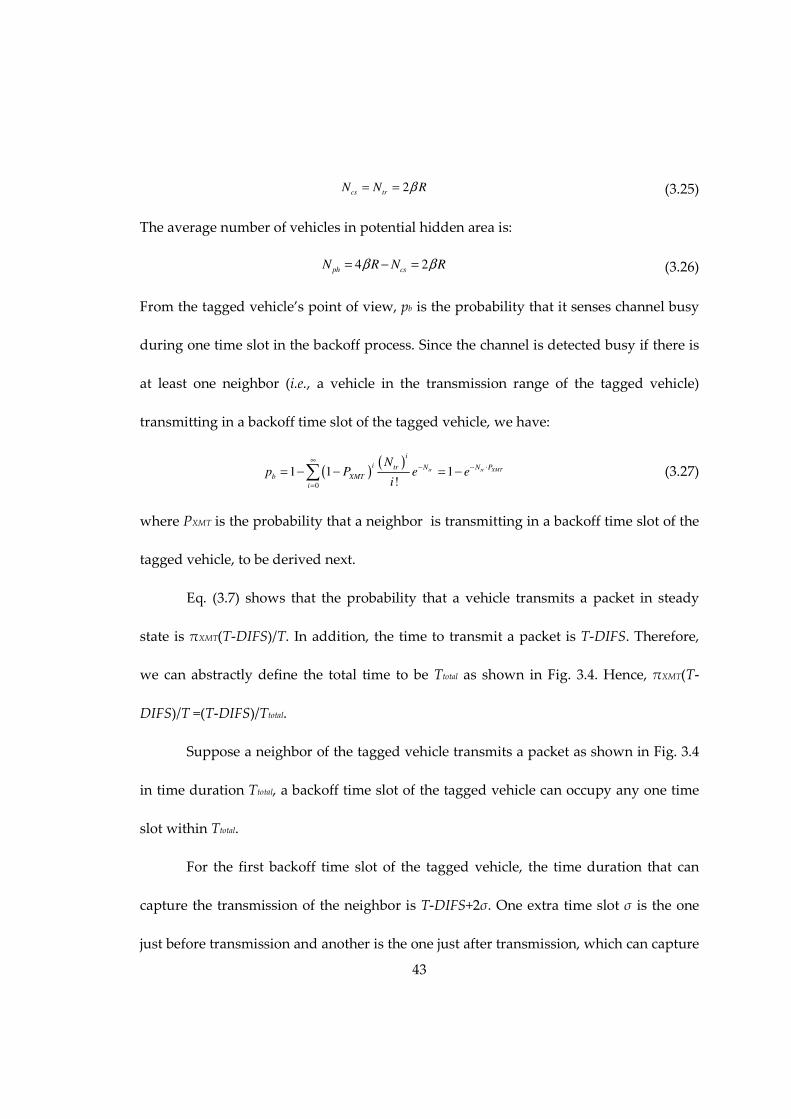
43

2cs tr

N N Rβ= = (3.25)

The average number of vehicles in potential hidden area is:

4 2ph cs

N R N Rβ β= − = (3.26)

From the tagged vehicle’s point of view, pb is the probability that it senses channel busy

during one time slot in the backoff process. Since the channel is detected busy if there is

at least one neighbor (i.e., a vehicle in the transmission range of the tagged vehicle)

transmitting in a backoff time slot of the tagged vehicle, we have:

( )( )

0

1 1 1!

tr tr XMT

i

i tr N N P

b XMT

i

Np P e e

i

∞− − ⋅

=

= − − = −∑ (3.27)

where PXMT is the probability that a neighbor is transmitting in a backoff time slot of the

tagged vehicle, to be derived next.

Eq. (3.7) shows that the probability that a vehicle transmits a packet in steady

state is πXMT(T-DIFS)/T. In addition, the time to transmit a packet is T-DIFS. Therefore,

we can abstractly define the total time to be Ttotal as shown in Fig. 3.4. Hence, πXMT(T-

DIFS)/T =(T-DIFS)/Ttotal.

Suppose a neighbor of the tagged vehicle transmits a packet as shown in Fig. 3.4

in time duration Ttotal, a backoff time slot of the tagged vehicle can occupy any one time

slot within Ttotal.

For the first backoff time slot of the tagged vehicle, the time duration that can

capture the transmission of the neighbor is T-DIFS+2σ. One extra time slot σ is the one

just before transmission and another is the one just after transmission, which can capture

44

the starting time instant and ending time instant of the packet transmission. Therefore,

the probability that a neighbor’s transmission is detected in the first backoff time slot of

the tagged vehicle is πXMT(T-DIFS+2σ)/T.

For a backoff time slot that is not the first backoff time slot of the tagged vehicle,

the time duration that captures the transmission of the neighbor is 2σ, which captures

the starting time instant of the transmission. This is because when the neighbor’s

transmission is detected in the first backoff time slot by the tagged vehicle, the backoff

Figure 3.4: Abstraction of the packet transmission time

Figure 3.5: Import graph for fixed point iteration

counter will suspend and wait until the end of this transmission for further decrement.

Therefore, if the first backoff time slot detects the transmission, there is no chance for the

later backoff time slots to detect the same transmission. As a result, the non-first backoff

time slot can only detect the transmission when the starting point of the transmission

falls within this time slot. Therefore, the probability that a neighbor’s transmission is

detected in non-first backoff time slot of the tagged vehicle is πXMT·2σ/T.

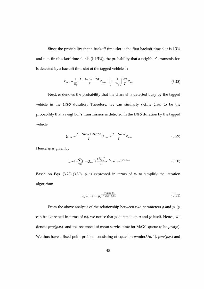
45

Since the probability that a backoff time slot is the first backoff time slot is 1/W0

and non-first backoff time slot is (1-1/W0), the probability that a neighbor’s transmission

is detected by a backoff time slot of the tagged vehicle is:

0 0

1 2 1 21

XMT XMT XMT

T DIFSP

W T W T

σ σπ π

− += ⋅ + − ⋅

(3.28)

Next, qb denotes the probability that the channel is detected busy by the tagged

vehicle in the DIFS duration. Therefore, we can similarly define QXMT to be the

probability that a neighbor’s transmission is detected in the DIFS duration by the tagged

vehicle.

2XMT XMT XMT

T DIFS DIFS T DIFSQ

T Tπ π

− + += = (3.29)

Hence, qb is given by:

( )( )

0

1 1 1!

tr tr XMT

i

i tr N N Q

b XMT

i

Nq Q e e

i

∞− − ⋅

=

= − − = −∑ (3.30)

Based on Eqs. (3.27)-(3.30), qb is expressed in terms of pb to simplify the iteration

algorithm:

( )( ) 0

021 1T DIFS W

T DIFS Wb bq p σ

+

− += − − (3.31)

From the above analysis of the relationship between two parameters ρ and pb (qb

can be expressed in terms of pb), we notice that pb depends on ρ and pb itself. Hence, we

denote pb=g(ρ,pb) and the reciprocal of mean service time for M/G/1 queue to be µ=h(pb).

We thus have a fixed point problem consisting of equation ρ=min(λ/µ, 1), pb=g(ρ,pb) and

46

µ=h(pb). The import graph [16] of this system of equations is shown in Fig. 3.5. We use

successive substitution to obtain a solution to the fixed-point.

Fixed-point iteration algorithm:

Step 1: Initialize ρ=1, which is the saturation condition;

Step 2: With ρ, solve pb according to Eqs. (3.27)(3.28)(3.7)(3.31);

Step 3: With pb, calculate service rate µ=1/E[S] according to Eq. (3.24);

Step 4: If λ<µ, ρ=λ/µ; otherwise, set ρ=1;

Step 5: If ρ converges, then stop the iteration algorithm; otherwise, go to step 2 with the

updated ρ.

By utilizing the fixed-point iteration algorithm, the parameters ρ, pb, qb, πXMT as

well as the mean and the variance of the service time can be determined, which are used

for the performance indices computation in the next section. The proofs for the existence,

uniqueness and convergence of the fixed-point iteration are given in the next subsection.

3.3.4 Existence, Uniqueness and Convergence of Fixed-point Iteration

In this section, we provide the proofs for the existence, uniqueness and

convergence [14][15] of the fixed point mentioned in Section 3.3.3. Since ρ depends on

the service time; the service time depends on pb; pb depends on ρ; hence, we have the

fixed point equation:

( )fρ ρ= (3.32)

47

( )( )

min 1,fλ

ρµ ρ

=

(3.33)

3.3.4.1 Existence

In In this section, Brouwer’s fixed-point theorem will be used to prove that ρ=f(ρ)

has a solution [14][18]. Brouwer’s fixed-point theorem states that if there exists a

compact, convex set C and there exists a continuous function f, such that if y∈C, then

f(y)∈C, then there exists a solution to the equation f(y)=y.

Since ρ is the probability that there are packets ready to transmit, ρ∈[0,1].

Therefore, we define C=[0,1].

According to Heine-Borel theorem [19], for a subset S of Euclidean space Rn, if S is

closed and bounded, S is a compact set. Therefore, C=[0,1] is a compact set. C is a convex

set [19] if λx+(1-λ)y∈C whenever x∈C, y∈C and λ∈[0,1]. Consider: z=λx+(1-λ)y. z≥0

because λ≥0, x≥0, (1-λ) ≥0, and y≥0. Since z is maximized when x=y=1 (since λ≥0 and (1-

λ) ≥0) to its maximum value 1, z≤1. Hence, C is a convex set.

Consider the function f over C. By definition, f(ρ)=min(1,λ/µ(ρ)), λ is positive. If ρ∈ [0,1], then pb∈ [0,1], µ>0 (according to the equations for pb(ρ) and µ(ρ)); hence,

f(ρ)=min(1,λ/µ(ρ)∈[0,1]. f is a continuous function if for each point ˆ Cρ ∈ ,

( ) ( )ˆˆlim f fρ ρ ρ ρ→ =

By definition,

( )( )ˆ ˆlim lim min 1,fρ ρ ρ ρ

λρ

µ ρ→ →

=

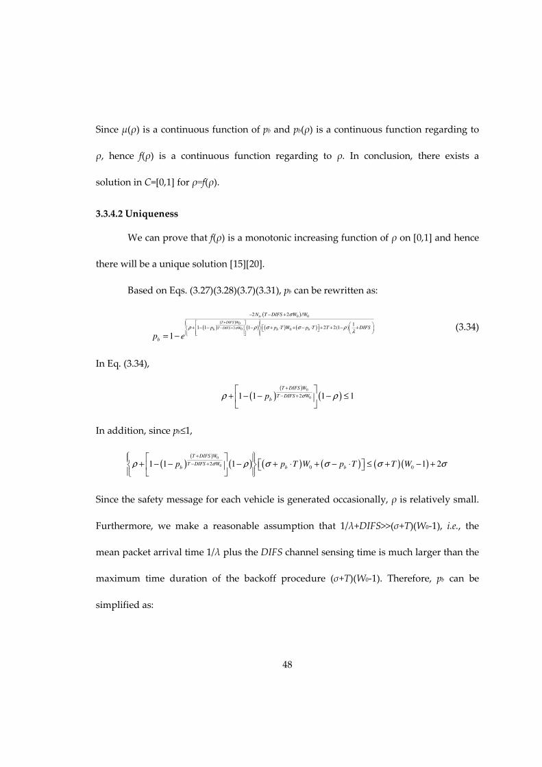
48

Since µ(ρ) is a continuous function of pb and pb(ρ) is a continuous function regarding to

ρ, hence f(ρ) is a continuous function regarding to ρ. In conclusion, there exists a

solution in C=[0,1] for ρ=f(ρ).

3.3.4.2 Uniqueness

We can prove that f(ρ) is a monotonic increasing function of ρ on [0,1] and hence

there will be a unique solution [15][20].

Based on Eqs. (3.27)(3.28)(3.7)(3.31), pb can be rewritten as:

( )

( )( )

( ) ( ) ( )

0 0

0

2 0 0

2 2 /

11 1 1 2 2(1 )

1

tr

T DIFS W

T DIFS Wb b b

N T DIFS W W

p p T W p T T DIFS

bp eσ

σ

ρ ρ σ σ ρλ

+

− +

− − +

+ − − − + ⋅ + − ⋅ + + − +

= − (3.34)

In Eq. (3.34),

( )( )

( )0

021 1 1 1T DIFS W

T DIFS Wb

p σρ ρ+

− +

+ − − − ≤

In addition, since pb≤1,

( )( )

( ) ( ) ( ) ( )( )0

020 01 1 1 1 2

T DIFS W

T DIFS Wb b b

p p T W p T T Wσρ ρ σ σ σ σ+

− +

+ − − − + ⋅ + − ⋅ ≤ + − +

Since the safety message for each vehicle is generated occasionally, ρ is relatively small.

Furthermore, we make a reasonable assumption that 1/λ+DIFS>>(σ+T)(W0-1), i.e., the

mean packet arrival time 1/λ plus the DIFS channel sensing time is much larger than the

maximum time duration of the backoff procedure (σ+T)(W0-1). Therefore, pb can be

simplified as:

49

( )0 02 /

1(1 )

1 e

trN T DIFS W W

T DIFS

bp

σ

σ ρλ

− − +

+ + − +

≈ − (3.35)

According to Eq. (3.35), if ρ increases, pb will increase given the condition that

1/λ+DIFS>>(σ+T)(W0-1). Hence, µ will decrease, and then, f(ρ)=min(1,λ/µ(ρ)) will

accordingly increase. Hence, f(ρ) is a monotone increasing function of ρ on [0,1].

Moreover, f(ρ)=min(1,λ/µ(ρ))>0, f(1) is also a value between 0 and 1. Therefore,

the solution of ρ=f(ρ) on [0,1] is unique.

3.3.4.3 Convergence

According to the fixed-point theorem: Let (X, d) be a complete metric space and f:

X->X be a map such that

( ) ( )( ) ( ), ' , 'd f x f x kd x x≤ (3.36)

for some 0≤k<1 and all x and x’ in X. Then f has a unique fixed point in X. Moreover, for

any x0 in X, the sequence of iterates x0, f(x0), f(f(x0)),… converges to the fixed point of f.

Therefore, we need to find a value of k (0≤k<1) to satisfy Eq. (3.36) to prove that

the fixed point converges.

According to Lagrange mean value theorem, if a function f(x) is continuous on the

closed interval [a, b] and differentiable within this range, then there exists x0, a<x0<b, such

that f(b)-f(a)=f’(x0)(b-a). Therefore, if we can find the upper bound of f’(x0), and prove 0≤

f’(x0) <1, we can prove the convergence of the fixed point.

50

Since f(ρ)=min(1,λ/µ(ρ)) in our model, to make f(ρ) differentiable in range [0,1],

we need to make sure λ<µ(ρ) for ρ∈[0,1], hence:

( )( ) ( )

( )( )

( )( ) ( )

( )( ) ( )

( ) ( ) ( )

0

0

0

0

0

0

( )

20

( )

20

1

1 2

2 1 1

1 1 1 2

2 1 1

e

b e

b b

b b

T DIFS W

T DIFS Wb b

T DIFS W

T DIFS Wb b

f

W p T q T

W p T q

W p T p T

W p T p

A

B

σ

σ

λβλρ

µ ρ λ β β

λ σ

λ σ

λ σ

λ σ

+

− +

+

− +

= =− −

− + ⋅ ⋅ + =− − + ⋅ ⋅ −

− + ⋅ ⋅ − − +

=

− − + ⋅ ⋅ −

=

(3.37)

where

( )( ) ( )

( )( ) ( )

0

0

0

0

( )

20

( )

20

1 1 1 2

2 1 1

T DIFS W

T DIFS Wb b

T DIFS W

T DIFS Wb b

A W p T p T

B W p T p

σ

σ

λ σ

λ σ

+

− +

+

− +

= − + ⋅ ⋅ − − +

= − − + ⋅ ⋅ −

Thus,

( ) ( )2

b b b b

b

dA dBB A

df df dp dp dp dp

d dp d dB

ρ ρ

ρ ρ ρ

⋅ − ⋅

= ⋅ = ⋅

( ) ( ) ( ) ( )0 0

0 0

( ) ( )102 2

0

0

( )1 1 1 1

2

T DIFS W T DIFS W

T DIFS W T DIFS Wb b b

b

T DIFS WdAW T p p T p

dp T DIFS Wσ σλ σ

σ

+ +−

− + − + +

= − − − + + ⋅ − − +

( ) ( ) ( ) ( )0 0

0 0

( ) ( )10

2 20

0

( )1 1 1

2

T DIFS W T DIFS W

T DIFS W T DIFS Wb b b

b

T DIFS WdBW T p p T p

dp T DIFS Wσ σλ σ

σ

+ +−

− + − ++

= − − − − + ⋅ − − +

(3.38)

Since pb∈[0,1], (dA/dpb·B-dB/dpb·A)/B2 is bounded according to Eq. (3.38). Denote the

upper bound as U1.

51

According to the theorem on differentiability, since dpb/dρ is differentiable, then

dpb/dρ is continuous [19]. Furthermore, according to the boundedness theorem [21], since

dpb/dρ is continuous on the compact space [0,1], there exists a real number U2 such that

dpb/dρ<=U2.

Therefore,

( )1 22

b b b

dA dBB A

df dp dp dpU U k

d dB

ρ

ρ ρ

⋅ − ⋅

= ⋅ ≤ ⋅ = (3.39)

Hence, if we choose reasonable parameters for λ, W0, T, DIFS, σ to satisfy 0≤k<1,

then k will be the Lipschitz constant of f and successive iterates x0, f(x0), f(f(x0)),… will

converge to the fixed point of f.

3.4 Performance Indices

3.4.1 Mean Transmission Delay

According to the Welch’s method [13], the steady-state expected number of

packets in the tagged vehicle’s queue (including the packet in the head of the queue that

is under service) is:

[ ]( )

( )( )

2 2 2 2 2 22 2

1 2 1 2 1

e e b be b b

b e b e b

E Qσ β σ βλβ σ βλ λ

λ β β λ β β λβ

+ − − += + ⋅ + ⋅

− − − − − (3.40)

Using Little’s law, the mean delay for a packet transmission is:

[ ][ ]E Q

E Dλ

= (3.41)

52

3.4.2 Packet Delivery Ratio

The PDR is defined as [5][7]: given a broadcast packet sent by the tagged vehicle,

the probability that all vehicles in its transmission range receive the packet successfully.

Taking account of hidden terminals, we have:

( ) ( )cs phPDR P N P N= (3.42)

where P(Ncs) is the probability that no vehicles in the transmission range of the tagged

vehicle transmits when the tagged vehicle starts transmission, and P(Nph) is the

probability that no transmissions from the vehicles in the potential hidden terminal area

collide with the broadcast packet from the tagged vehicle.

P(Ncs) can also be interpreted as the non-concurrent transmission probability, i.e.,

two packets do not start transmission at the same time. Since DCF employs a discrete-

time backoff scheme, if the backoff process is involved, a vehicle is only allowed to

transmit at the beginning of each slot time after an idle DIFS time duration. Therefore, if

the tagged vehicle has not gone through the backoff process before transmitting the

packet (with probability (1-ρ)(1-qb)), the concurrent transmission will not occur.

Otherwise, the packet transmission is synchronized to the beginning of a slot time, and

concurrent transmission may occur if other vehicles’ transmission is also synchronized

by the backoff process. From the model, we know that the probability that a neighbor

starts to transmit a packet at the beginning of the same time slot with the tagged vehicle

is π0= πXMT•σ/T. This is because the sojourn time in state 0 is one time slot σ as shown in

53

the SMP model, hence, π0 is the probability that a vehicle starts to transmit in the

beginning of a time slot immediately after the backoff process. Hence, P(Ncs) is:

( ) ( ) ( ) ( )( ) ( ) ( )( )

( ) ( ) ( ) ( )( )0

1

0

0

1

11 1 1 1 1 1

!

1 1 1 1 1

cs

cs

i

i Ncs

cs b b

i

N

b b

NP N q e q

i

q e qπ

ρ π ρ

ρ ρ

∞− −

=

− −

−= − − − ⋅ − + − −

= − − − ⋅ + − −

∑ (3.43)

Since the transmission time for a packet is T-DIFS=E[PA]/Rd+TH+δ, the event that

a transmission from hidden terminals collides with the tagged vehicle’s transmission

only happens when hidden terminals start to transmit during the vulnerable period 2(T-

DIFS)=2(E[PA]/Rd+TH+δ) [7]. Using πXMT=T/Ttotal as an abstraction of the steady state

behavior shown in Fig. 3.4, the probability that a vehicle starts to transmit during the

vulnerable period of hidden terminal transmissions [7] is:

2( ) 2( )XMT

T DIFS T DIFS

Ttotal Tπ

− −= (3.44)

Therefore,

( )( ) 2( )

0

2( )1

!

ph XMT

ph

ii T DIFS N

ph N Tph XMT

i

NT DIFSP N e e

T i

π

π− − ⋅ ⋅∞

−

=

− = − ⋅ =

∑ (3.45)

Hence, based on Eqs. (3.42)(3.43)(3.45), the PDR can be computed. From the

analytic-numerical results demonstrated in Section 3.5, we can see that the hidden

terminals problem has more impact than concurrent transmissions on the PDR.

54

3.4.3 Packet Reception Ratio

Packet reception ratio (PRR) is defined as the percentage of nodes that

successfully receive a packet from the tagged node among the receivers being

investigated at the moment that the packet is sent out [7].

Similar to the computation for PDR, we consider both the concurrent

transmission and hidden terminal effects while computing PRR. Therefore,

htccPRRPRRPRR = (3.46)

The impact of the concurrent transmission and hidden terminals will be evaluated in the

following two sections.

a. Impact of concurrent transmission

Transmissions from nodes within a distance R away from the tagged node in the

meantime at which the tagged node transmits may cause collisions. When the tagged

node starts transmission in the beginning of a slot time, collisions will take place if any

node in the transmission range of the tagged node starts transmission in the beginning

of the same time slot. As shown in Fig. 3.6, any node transmitting on the right hand side

of the tagged node (i.e., node in L1={x|x∈[0, R]}) will result in failure of all nodes in L1

receiving the broadcast packet. Hence, ratio of successfully receiving nodes in the range

L1 can be expressed as:

01

0

0

( )(1 )

!

iRi R

cc

i

RPRR e e

i

β πββπ

∞−−

=

= − =∑ (3.47)

55

On the other hand, transmissions from any node on the left hand side of the

tagged node (i.e., node in L2={x|x∈[-R, 0]}) will only result in failure of some of the

nodes receiving the broadcast packet in L1. Similar to analysis of the hidden terminal

impact, the ratio of successful receiving nodes due to any transmission in L2 depends on

the position of the closest node transmitting in L2 to the tagged node. Denote Y as a

random variable that represents the distance from the closest node transmitting in L2 (B

in Fig. 3.6) to the outer boundary of range L2. Let Rt be the range where no station

transmits, so that

Figure 3.6: PRR computation

[ ]0

( ) (none of nodes in transmits in a slot)t

k

P Y y P k R∞

=

≤ =∑ (3.48)

Rt={x|x∈[-R+y,0]]. Then the CDF for Y is: Eq. (3.48) is the probability that the closest

interfering node in L2 is at least (R-y) away from the transmitter; i.e., the probability that

no nodes within Rt transmit in the meantime the tagged node starts to transmit. Hence,

we have:

0( )( )

0

0

( ( ))( ) (1 )

!

kR yk R y

k

R yP Y y e e

k

β πββπ

∞− −− −

=

−≤ = − =∑ (3.49)

56

Thus, the expected number of failed nodes in L1 due to concurrent transmission of nodes

in L2 can be expressed as:

( )0 0( )2

00 0

0

1( ) 1

R RR y R

hNF yP y Y y dy y e dy R eβ π βπβ β π β

π− − −= ≤ ≤ + = = − −∫ ∫ (3.50)

Therefore, the percentage of receivers in L1 that are free from collisions caused by the

concurrent transmissions of nodes in the range L2 is:

02

0

1(1 )

Rh

cc

R NFPRR e

R R

β πβ

β β π−−

= = − (3.51)

Define PRRcc as the percentage of receivers in L1 that are free from collisions caused by

the concurrent transmissions of nodes in the range {x|x∈[-R, R]}. If the tagged vehicle

transmits the packet without going through the backoff process, with probability (1-ρ)(1-

qb), concurrent transmission will not occur. Otherwise, concurrent transmissions may

occur. Therefore,

( ) ( ) ( )( )

( )( ) ( )( )0

0

1 2

0

1 1 1 1 1

(1 ) 1 1 1 1 1

cc cc cc b b

RR

b b

PRR PRR PRR q q

ee q q

R

β πβ π

ρ ρ

ρ ρβ π

−−

= ⋅ ⋅ − − − + − −

= − − − − + − −

(3.52)

b. Impact of hidden terminals

We observe that the ratio of receivers affected by the hidden terminals only

depends on the position of the hidden node (referred as hidden crucial node) that has

the closest distance to boundary of the transmitter’s sensing range among all the

transmitting nodes in the potential hidden terminal area. Denote X as a random variable

that represents the distance from the hidden crucial node (A in Fig. 3.6) to the outer

57

boundary of {x|x∈[0, 2R]}. Let Rs be the range in the potential hidden terminal area,

where no node transmits, such that Rs={x|x∈[lcs, 2R-x]}, where lcs=Ncs/(2β) is carrier

sensing range of a node in the network.

Then the cumulative distribution function (CDF) for X is:

[ ]

( )( )( )

( )

( )

0

0

( ) (none of nodes in transmits during tagged node's transmission )

22( )1 exp 2

!

2 ( ) 2exp

exp (2 )

s

k

kk

cs

XMT cs

k

XMT cs

cs

P X x P k R

R l xT DIFSR l x

T i

T DIFS R l x

T

C R l x

βπ β

π β

∞

=

∞

=

≤ =

− − − = − ⋅ − − −

− − − = −

= − − −

∑

∑ (3.53)

where C=2πXMTβ(T-DIFS)/T. Thus, the expected number of failed nodes in [0, R] due to

the hidden terminal problem can be expressed as:

{ } ( ) ( )( )

2

0

2

0

( )

( ) 2 1 exp 2

cs

cs

R l

h X

R l

cs cs

NF xf x dx

xd P X x R l c R lC

β

ββ β

−

−

=

= ≤ = − − − − −

∫

∫ (3.54)

Therefore, the percentage of receivers that are free from collisions caused by hidden

terminal problem is:

( )1

1 exp (2 )h cs

ht cs

R NF l RPRR C R l

R R RC

β

β

− −= = + − − −

(3.55)

Hence, based on Eqs. (3.46)(3.52)(3.55), the PRR can be computed. Similar to the

case of the PDR, the hidden terminals problem also has more impact than concurrent

transmissions on the PRR, as shown in Section 3.5.

58

3.5 Numerical and Simulation Results

The computation for analytic models and corresponding simulations are

conducted in Matlab. Note that the analytic model consists of decomposition and fixed-

point iteration while the simulative solution does not. All other assumptions are the

same in the simulation and analytic models. The results show the high accuracy of our

decomposition-based analytic approximation. We consider a freeway system where the

number of vehicles is Poisson distributed. Each vehicle on the road is equipped with

DSRC wireless capability. The control channel of DSRC is exclusively used for safety

related broadcast communication. Table 3.1 shows the parameters used in this work,

which reflect typical DSRC network settings in [1]. In addition, the variables in Table 3.1

such as the packet arrival rate and the average packet length are chosen according to [42]

to satisfy the maximum channel utilization limitation of IEEE 802.11, which is required

to be 54%-66% in the absence of hidden terminals. For unrealistic situations that exceed

such limits, our proposed model in this work may not apply. Under such channel

saturation conditions, other models have been developed earlier [23][43].

Table 3.1: DSRC communication parameter

Parameters Values Parameters Values

Tx range R 500 m Propagation delay δ 0 µs

Average Packet

Length E[PA] variable

Variance of Packet Length

Var[PA] 0

PHY preamble 40 µs PLCP header 4 µs

MAC header 272 bits CWMin W0-1 15

Packet arrival rate λ variable Vehicle density β variable

Slot time σ 16 µs DIFS 64 µs

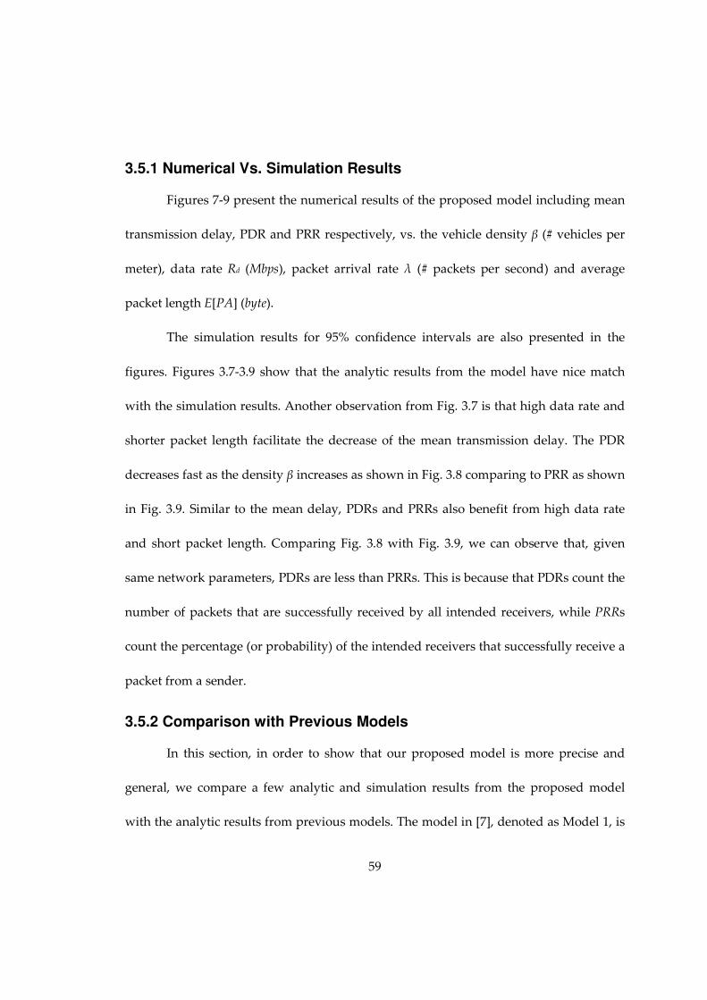
59

3.5.1 Numerical Vs. Simulation Results

Figures 7-9 present the numerical results of the proposed model including mean

transmission delay, PDR and PRR respectively, vs. the vehicle density β (# vehicles per

meter), data rate Rd (Mbps), packet arrival rate λ (# packets per second) and average

packet length E[PA] (byte).

The simulation results for 95% confidence intervals are also presented in the

figures. Figures 3.7-3.9 show that the analytic results from the model have nice match

with the simulation results. Another observation from Fig. 3.7 is that high data rate and

shorter packet length facilitate the decrease of the mean transmission delay. The PDR

decreases fast as the density β increases as shown in Fig. 3.8 comparing to PRR as shown

in Fig. 3.9. Similar to the mean delay, PDRs and PRRs also benefit from high data rate

and short packet length. Comparing Fig. 3.8 with Fig. 3.9, we can observe that, given

same network parameters, PDRs are less than PRRs. This is because that PDRs count the

number of packets that are successfully received by all intended receivers, while PRRs

count the percentage (or probability) of the intended receivers that successfully receive a

packet from a sender.

3.5.2 Comparison with Previous Models

In this section, in order to show that our proposed model is more precise and

general, we compare a few analytic and simulation results from the proposed model

with the analytic results from previous models. The model in [7], denoted as Model 1, is

60

used for the mean delay and PDR comparison. The model in [39], denoted as Model 2, is

used for PRR (although referred as PDR in Eq. 19 of the work) comparison. Figures 10-12

present the mean transmission delay, PDR and PRR respectively for these models along

with the simulation results for 95% confidence intervals.

0 0.02 0.04 0.06 0.08 0.1 0.12 0.14 0.16 0.18 0.21

2

3

4

x 10-4

Density (No. of Vehicles/meter)

Mean D

ela

y (

second)

Rd=12,lam=2,E[PA]=200,model




Figure 3.7: Mean delay

0.02 0.04 0.06 0.08 0.1 0.12 0.14 0.16 0.18 0.20.4

0.5

0.6

0.7

0.8

0.9

1

Density (vehicles/meter)

Packet

Deliv

ery

Ratio





Figure 3.8: PDR

0.02 0.04 0.06 0.08 0.1 0.12 0.14 0.16 0.18 0.20.6

0.65

0.7

0.75

0.8

0.85

0.9

0.95

1


Packet

Reception R

atio





Figure 3.9: PRR

Fig. 3.10 shows that, for the same input parameters, the new model obtains lower

mean delay than the model in [7]. This is mainly since the new SMP model considers the

61

fact that a packet can be directly transmitted without undergoing backoff process, which

was ignored in [7]. In addition, the PDR results in Fig. 3.11 also show that new model

has better match with simulations than Model 1. The PRR computation method in Eq. 19

in [39] (i.e., Model 2) is shown as below (A few symbol adjustments are made according

to our definitions in this work):

( )0

0

1exp 2 1 exp 2

2XMT

XMT

T DIFSPRR R R

T DIFS TR

T

πβ π β π

β π

− − = ⋅ − ⋅ − − ⋅ ⋅ − ⋅ ⋅

(3.56)

The PRR results comparison is illustrated in Fig. 3.12 and the proposed new model

shows better match than Model 2.

For better illustration, the relative errors of these models with simulation results

are presented in Table 3.2-3.4, with input parameters Rd=24 Mbps, λ=10 packets/second,

E[PA]=200 bytes. Table 3.2 shows that the packet mean transmission delay obtained

from our proposed new model matches very well with the simulation (relative error is

less than 2%), whereas the Model 1 without considering the packet transmission not

undergoing backoff procedure deviates from the simulation results significantly

(relative error is more than 48%). Table 3.3 also shows that the PDRs obtained from the

new model (relative error is less than 2%) match better with the simulation than Model

1(relative error is less than 8%). Table 3.4 shows that the PRRs from the new model

(relative error is less than 1%) match better than Model 2 (relative error is less than 2%).

62

0 0.02 0.04 0.06 0.08 0.1 0.12 0.14 0.16 0.18 0.20

1

2

3

4

5

x 10-4


Mean D

ela

y (second)

Rd=24,lam=10,E[PA]=200,new model


Rd=24,lam=10,E[PA]=200,model 1


Figure 3.10: Mean delay comparison

0.02 0.04 0.06 0.08 0.1 0.12 0.14 0.16 0.18 0.2

0.4

0.5

0.6

0.7

0.8

0.9

1


Packet

Deliv

ery

Ratio





Figure 3.11: PDR comparison

0.02 0.04 0.06 0.08 0.1 0.12 0.14 0.16 0.18 0.20.8

0.82

0.84

0.86

0.88

0.9

0.92

0.94

0.96

0.98

1


Packet

Reception R

atio





Figure 3.12: PRR comparison

Table 3.2: Mean delay E[D] comparisons

Density 0.02 0.06 0.1 0.14 0.18 0.2

Simulation(ms) 0.1938 0.2090 0.2265 0.2422 0.2608 0.2651

Model 1(ms) 0.3114 0.3269 0.3444 0.3642 0.3866 0.3989

new model(ms) 0.1924 0.2064 0.2227 0.2407 0.2602 0.2703

63

Table 3.3: PDR comparison

Density 0.02 0.06 0.1 0.14 0.18 0.2

Simulation 0.9568 0.8622 0.7788 0.7018 0.6271 0.6032

Model 1 0.9469 0.8465 0.7539 0.6687 0.5905 0.5540

new model 0.9523 0.8628 0.7809 0.7062 0.6381 0.6065

Table 3.4: PRR comparison

Density 0.02 0.06 0.1 0.14 0.18 0.2

Simulation 0.9888 0.9646 0.9440 0.9160 0.8963 0.8884

Model 2 0.9846 0.9549 0.9264 0.8988 0.8723 0.8594

new model 0.9878 0.9633 0.9389 0.9148 0.8909 0.8791

3.5.3 Impact Comparison between Concurrent Transmission and Hidden Terminals

As per Sections 3.4.2 and 3.4.3, the PDR and PRR are influenced by both

concurrent transmission and hidden terminals. In order to determine which factor is

more critical for DSRC safety message transmission, we conduct the impact comparison

between the concurrent transmission and hidden terminals in this section. Fig. 3.13

presents the PDR according to Eq. (3.42), where P(Ncs) incorporates the impact of

concurrent transmission and P(Nph) incorporates the impact of hidden terminals.

Similarly, Fig. 3.14 presents the PRR according to Eq. (3.46), where PRRcc incorporates

the impact of concurrent transmission and PRRht incorporates the impact of hidden

terminals. As shown in these figures, the PDR and PRR are dominated by the hidden

terminals problem, whereas the concurrent transmission has little influence on the PDR

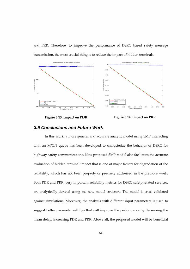
64

and PRR. Therefore, to improve the performance of DSRC based safety message

transmission, the most crucial thing is to reduce the impact of hidden terminals.

0.02 0.04 0.06 0.08 0.1 0.12 0.14 0.16 0.18 0.20.85

0.9

0.95

1


Packet

Delivery

Ratio

Impact comparison with Rd=12,lam=2,E[PA]=200

PDR=P(Ncs)*P(Nph)

P(Ncs)

P(Nph)

Figure 3.13: Impact on PDR

0.02 0.04 0.06 0.08 0.1 0.12 0.14 0.16 0.18 0.20.96

0.965

0.97

0.975

0.98

0.985

0.99

0.995

1


Packet

Reception R

atio

Impact comparison with Rd=12,lam=2,E[PA]=200

PDR=PRRcc*PRRht

PRRcc

PRRht

Figure 3.14: Impact on PRR

3.6 Conclusions and Future Work

In this work, a more general and accurate analytic model using SMP interacting

with an M/G/1 queue has been developed to characterize the behavior of DSRC for

highway safety communications. New proposed SMP model also facilitates the accurate

evaluation of hidden terminal impact that is one of major factors for degradation of the

reliability, which has not been properly or precisely addressed in the previous work.

Both PDR and PRR, very important reliability metrics for DSRC safety-related services,

are analytically derived using the new model structure. The model is cross validated

against simulations. Moreover, the analysis with different input parameters is used to

suggest better parameter settings that will improve the performance by decreasing the

mean delay, increasing PDR and PRR. Above all, the proposed model will be beneficial

65

to the analysis, design, and network parameter optimization for required performance

and reliability of DSRC VANET for safety-related services. Based on the proposed

model, more practical models for more applications can be developed.

In the future, the assumptions made in Section 3.2 will be gradually relaxed to

reflect the real world scenario. The analytic model will be extended to incorporate

different packet arrival processes such as Markov modulated Poisson process (MMPP),

Markovian arrival process (MAP) instead of Poisson arrivals. Different types of safety

messages over the control channel will be considered. In a tagged vehicle, we can use

different queues to store different types of messages and construct separate SMP models

for each type of safety message service. These separated SMP models will interact with

each other and also with their own corresponding M/G/1 queue. Fixed-point iteration

will then be used to obtain the converged solution. Therefore, the extension of our

model for multiple services is quite straightforward. Moreover, channel

shadowing/fading, capturing effect and vehicle mobility will be incorporated. 1-D

highway will be extended to 2-D case to model the intersecting roads, parallel lines in

highways, square grid for downtown area, etc. Besides one-hop direct broadcast

transmission strategy, multi-hop and multi-cycle transmission strategy will also be

considered in future.

66

4. Periodic Beacon Messages Evaluation

4.1 Motivation

Transportation safety is one of the most critical features addressed in Intelligent

Transportation System (ITS) [44]. In wireless vehicular communications, various safety

applications such as collision avoidance and safety warnings are expected to be enabled

to prevent and reduce traffic accidents. To support these safety applications, periodic

beacon message, i.e., basic safety message (BSM) [45][46], is widely used in dedicated

short range communications (DSRC). Beacon message contains information related to

the state of vehicle (e.g., position, velocity and direction) and such messages are

periodically exchanged with nearby vehicles in a broadcast fashion. Based on such

information, various safety applications are able to assist drivers to take appropriate

actions to prevent collisions when emergencies occur (e.g., rear-end collision warning,

slow vehicle indication, etc.). Hence, beacon messages are required to be transmitted

both in a timely and reliable manner to ensure the quality of service (QoS) for various

applications.

The MAC-level performance of the beacon message dissemination in DSRC

system has been studied in [47][48][49] based on discrete event simulations. Analytic

models are more suited in comparing design alternatives and exploring a large

parameter space. Several analytic models are developed in [8][50][51] to characterize the

MAC layer behavior of beacon message transmission and important performance

67

metrics are evaluated. However, Ma [8] used Poisson arrivals to approximate the

periodic generations of beacon messages (i.e., routine message), which leads to

inaccuracies. Vinel [50] considered the deterministic behavior of beacon generations by

modeling each vehicle as a D/M/1 queuing system. Infinite queue size is assumed by

them where out-dated information replacement is not considered. Bastani [51]

accounted for the periodic nature of beacon message generations and new message

canceling out old message phenomena, which is more reasonable and practical.

However, their model does not accurately capture the periodic beacon message

generation since it separates the periodic message generation from the message channel

contention and transmission behavior, although these behaviors are closely correlated.

According to [46], beacon messages are periodically generated to broadcast vehicle’s

status information. However, for the model presented in [51], the time interval between

the previous message finishing its transmission and the generation of the next message

is fixed beaconing period, which implies that the message generation is no longer

periodic since a message transmission time varies according to the channel’s status.

Hence, model in [51] cannot precisely capture the periodic beacon message generations.

In addition, all the above models are based on discrete-time Markov chain (DTMC) and

ignore the continuous time system behavior, which leads to approximations.

68

(a) Interactions between vehicles

(b) Models from one tagged vehicle’s perspective

Figure 4.1: Model capturing interactions between vehicles

In this chapter, we extend the work in [12][52] and develop a detailed and

accurate interacting semi-Markov Process (SMP) model [9] to incorporate periodic

generations as well as out-dated information replacement behavior for beacon messages.

Compared to the M/G/1 FCFS (first come first served) queuing model in our previous

work [52] in chapter 2, the generation and service of beacon messages in each vehicle in

this chapter is modeled by a D/G/1/1 LCFS (last come first served) queue with

preemption as shown in Fig. 4.1(a). In this notation, “D” represents that the message

inter-arrival time is deterministic. “G” represents that the service time has an arbitrary

distribution. The first “1” represents that there is only one server. The second “1”

represents that the queue size is one (i.e., no queuing). This queue is a LCFS preemption

queue because out-dated beacon message will be replaced by the next message to ensure

that the message to be sent in a vehicle is always up to date. Therefore, the overall model

is a set of interacting D/G/1/1 LCFS queues, one for each vehicle. The interaction is that

the server is shared as it is the contention medium/channel. To develop a tractable

69

analytic approximation, we use a semi-Markov process model to capture the shared

server’s behavior from one tagged vehicle’s perspective, which incorporates the

behavior of this tagged vehicle and the influences from other vehicles as shown in Fig.

4.1(b). This SMP model is accurate and comprehensive since it closely follows the

operational flow specified by DCF in IEEE 802.11p shown in Fig. 2.1. In addition, SMP

model with absorbing state is constructed to derive the message service time

distribution via Laplace–Stieltjes transform (LST). Due to the interactions between the

SMP models of different vehicles, fixed-point iteration [10][10] method is utilized to

obtain the converged solution in steady state. MAC-level performance metrics including

mean delay, packet delivery ratio (PDR), packet reception ratio (PRR) and normalized

channel throughput are derived. The proposed approximation is verified through

extensive simulations and compared with previous models for Poisson packet arrivals

and with infinite queue scenarios (i.e., M/G/1 FCFS queue) [52] and Bastani’s model in

[51].

Even though the MAC-level performance metrics play an important role for

understanding the packet transmission behavior and evaluating the efficiency of a

protocol, the application-level performance metrics are also essential to be addressed to

ensure the QoS of safety and non-safety applications because performance requirements

are typically given in terms of application-level metrics as opposed to packet-level

metrics. Efforts have been made in previous work [53][54][55] to characterize the

70

application-level performance metrics for specifying the application performance

requirements. Bai et al. [53] characterized Region of Interest (ROI) of VANET

applications into three qualitative levels: long, medium and short. In addition, the

application-level latency and application-level T-window reliability (TWR) (i.e., the

probability to successfully receive at least one packet during tolerance time window T)

were also proposed in [53] to guide performance requirements in terms of application-

level metrics. An et al. [54] proposed that the application requirements can be specified

as awareness range and awareness probability. The awareness probability generalized

the idea of TWR as the probability to successfully receive at least n packets in the

tolerance time window T. Awareness range is defined as the maximum distance at

which the awareness probability is greater than or equal to a certain threshold. The

authors in [55] defined the invisible neighbor problem and proposed to minimize the

total number of invisible neighbors over a certain time window to ensure the QoS of the

vehicle’s safety applications.

In this chapter, we adopt the definitions of Region of Interest, application-level

latency, T-window reliability, awareness probability and invisible neighbors from

previous work to characterize the application performance requirements. The

corresponding analytic results are derived based on the newly proposed interacting

SMP model for periodic beacon messages. Based on such analytic models for

application-level performance metrics, we provide insights on network parameter

71

settings to satisfy performance requirements for various applications. Furthermore,

three typical safety applications including slow vehicle indication, emergency vehicle

warning and rear-end collision warning are analyzed to assess whether their

performance requirement can be satisfied or not under a given DSRC network

parameters setting.

The key contributions of this chapter are six-fold: 1) Periodic beacon message

generation and out-dated message replacement behavior are incorporated into a

detailed and accurate analytic model, which closely follows the operational flow

specified by DCF in IEEE 802.11p; 2) Beacon message service time distribution is first

derived using Laplace–Stieltjes transform, based on which the mean service time is

computed; 3) Normalized channel throughput is derived for better understanding of

channel conditions under various input parameters; 4) Analytic results for a vehicle with

periodic beacon message generation and out-dated message replacement (i.e., D/G/1/1

LCFS queue) are compared to those for a vehicle model in [52] with Poisson message

arrivals and an infinite queue (i.e., M/G/1 FCFS queue) and Bastani’ model [51]; 5)

Application-level performance metrics including application-level latency, T-window

reliability, awareness probability, and the average number of invisible neighbors are

derived based on the newly proposed interacting SMP model; 6) Three typical safety-

applications are evaluated to assess whether their performance requirement can be met

or not under a given DSRC network parameters setting.

72


Several assumptions are made in the broadcast system to produce analytically

tractable yet a high fidelity model. The vehicular ad hoc network is considered to be

one-dimensional (1-D) for traffic on highway [9]. The number of vehicles in a line is

assumed to be Poisson distributed with parameter β (vehicle density), i.e., the

probability P(i, l) of finding i vehicles in a lane of length l is given by Eq. (3.1). In

addition, we assume all vehicles have the same transmission range, receiving range and

carrier sensing range R to simplify the analysis. Furthermore, an out-dated beacon

message is replaced by the new message. In other words, if the previous message has

not been transmitted when the new message is generated in a vehicle, the previous

message will be replaced by the next packet. This assumption is made since a beacon

message contains information such as the position, the velocity and the direction, etc.,

that needs to be updated periodically. Therefore, different from event-driven safety

messages that are too important to be replaced, no queueing of messages is needed for

the periodic beacon messages. Channel shadowing or fading, vehicle mobility and

capture effect of transmissions are not considered in this chapter. One more assumption

is that only beacon message service in the control channel (CCH) is considered in the

model.

73

4.3 Analytic Models

4.3.1 Overall Model

The overall system behavior is that of multiple vehicles competing for the

channel resource to transmit their own beacon messages over the CCH. Due to such

interactions between vehicles, the whole system can be captured by a Generalized Semi-

Markov Processes (GSMP) [56][57], which is a set of interacting semi-Markov processes.

Even assuming that all sojourn times are exponentially distributed, a single GSMP

model to analyze system behavior faces state explosion problem when the number of

vehicles is large. For example, suppose there are 100 vehicles in the system to be

analyzed, and each vehicle’s maximal backoff counter is 15, the GSMP model will

contain at least 15100 states (can be more due to channel sensing and backoff frozen

states) to capture the whole system behavior. First, there is no known analytic solution

to a GSMP; it can be either solved using discrete-event simulation or phase-type

expansion for all non-exponential distributions need to be carried out, in which case the

state space will get even bigger. We use model decomposition to develop a tractable

analytic model of such a complex system, denoted as ISP (Interacting Stochastic

Processes). This newly proposed ISP model and GSMP model are both based on a set of

interacting semi-Markov processes. The distinction is that: in GSMP model, the

interactions are at the level of events while for the ISP model, solutions of one SMP

74

provide parameters to the others. This decomposition is what makes our proposed ISP

approach analytically tractable while GSMP is not.

Figure 4.2: Import graph for the overall method

In this chapter, we decompose the overall model of the whole system and

develop a detailed SMP model in Section 4.3.2 that directly captures the channel

contention and backoff behavior from a single vehicle’s perspective. The influences from

other vehicles are incorporated into this single vehicle SMP model through four model

parameters (Pf, pb, qb, rb in Fig. 4.3) remaining to be determined. By solving the SMP

model, we can obtain the fully symbolic solution for the steady-state probability that a

single vehicle transmits. Based on a single vehicle’s behavior, three model parameters

(pb, qb, rb in Fig. 4.3) that capture the degree of channel contention from multiple vehicles

are derived. The one remaining model parameter (Pf in Fig. 4.3) is related to the out-

dated message replacement behavior, and hence the message service time distribution

needs to be derived first to determine whether a message will be replaced by the next

one or not. We propose Laplace–Stieltjes transform method over a modified SMP model

in Section 4.3.3 to derive a formula for this service time distribution and subsequently

derive the related model parameter. Since these four model parameters are inter-

75

dependent on each other, fixed-point iteration method is used to obtain converged

numerical solutions in Section 4.3.4. The import graph [16] for such overall method is

shown in Fig. 4.2. Let the SMP model in Section 4.3.2 be denoted by ISMP (Irreducible

SMP) and the modified SMP model with absorbing state in Section 4.3.3 be denoted by

SMPA. The results produced by these models are presented within rectangles in Fig. 4.2.

4.3.2 SMP Model

The behavior of a tagged vehicle is characterized using the irreducible SMP

model in Fig. 4.3. The channel sensing, backoff and transmission behavior matches well

with the flow chart shown in Fig. 2.1. The tagged vehicle is in idle state if there is no

packet. After a packet is generated, the vehicle senses channel activity for DIFS time

period, which is represented by state CS1. If the channel is detected not busy during this

period (with probability 1-qb), the vehicle goes from idle state to TX state, which means

that a packet is transmitting. Otherwise, the vehicle will defer until channel is idle for

DIFS duration represented by state DCS. Such deference behavior for the tagged vehicle

includes two parts: waiting for the current packet in the channel finishing transmission

and waiting for subsequent transmissions if any from other neighbors within its

receiving range. The self-loop for state DCS represents the phenomena in Fig. 4.6 that the

tagged vehicle (vehicle B) waits for the current packet (from vehicle A) in the channel

finishing transmission, and then senses the channel for DIFS time, which captures the

transmission from another vehicle (vehicle C) and leads to further deference. The

76

probability that the tagged vehicle detects another neighbor’s transmission during DIFS

time is denoted as rb. If no other neighbors’ transmission is detected, the tagged vehicle

will start backoff procedure and randomly choose a backoff counter in the range [0, W-

1], where W=CW+1 is the backoff window size. The backoff counter will be decreased by

one if the channel is detected to be idle for a time slot of duration σ (with probability 1-

pb), which is captured by the transition from state W-i to state W-i-1. If the channel is

busy during a backoff time slot of duration σ (i.e., another vehicle starts to transmit a

packet during this time slot), the backoff counter of the tagged vehicle will be

suspended, which represented by the transition from state W-i to DW-i-1 with probability

pb. Similar to state DCS, state DW-i-1 also contains self-loop because other neighbors’

transmission can lead to further deference of the tagged vehicle. When the backoff

counter reaches zero, the packet will directly be transmitted (an SMP transition occurs

from state 0 to state TX with probability one). In TX state, a packet is transmitting. To

capture the out-dated packet replacement behavior, which can happen during any state

except state TX and idle, we simplify the model by considering the replacement after

state TX. If the current packet has not been replaced by the next packet (with probability

1-Pf), the SMP goes to state idle. Otherwise, this current packet is out-dated and replaced

by the next incoming packet. Hence, the tagged vehicle starts the service for the next

packet immediately and senses the channel for DIFS time (state CS2) and goes through

the backoff procedure before it transmits the next packet.

77

Figure 4.3: SMP model for 802.11p beacon broadcast

Compared to the SMP model in [52], the newly proposed SMP model captures

more detailed DCF behavior for periodic beacon message transmission by adding more

states and self-loop structure. In addition, out-dated message replacement behavior is

incorporated into the model by the newly introduced model parameter Pf. Therefore, the

sojourn times and steady-state solutions are totally different from that in [52] although

similar computation procedure is used.


model are:

78

1

2

3 1 2

4

5 0 1 2

,

, , ,

0 0

1, 2, , 1

j j CS

W

A j TX

A j idle

A j CS CS

E T A j D

A j D D D

j

j W

τ

σ

−

=

= =

= = = = =

= −

L

L

(4.1)

2

1

0j j

j UVar T

B j idleθ

∈ = = =

(4.2)

where

[ ]

( )

1

2

3

4 1

5 1

/

/ 2

d HA PL R T

A E S

A DIFS

A A DIFS

A A DIFS

δ

τ

= + +

= −

= = + = +

[ ]1B Var S=

{ }1 2 0 1 2, , , , , , , ,0,1,2, , 1CS WU TX CS CS D D D D W−= −L L

PL represents the packet length. Rd presents the data rate. Hence, PL/Rd is the time to

transmit the packet. TH presents the time to transmit the packet header including

physical layer header and MAC layer header. δ is the propagation delay. E[S] and Var[S]

are the mean and variance of the overall message service time, which will be derived

later. The sojourn time in state idle is the packet inter-arrival time excluding the packet

service time.

As in [52], the embedded DTMC is first solved for its steady-state probabilities:

79

( )

( )

( )( )

( )

( )( ) ( )

( )( ) ( )

( ) ( )

1 2

1

1

1 1

1 1

1

1

0,1, 1

10,1, 2

1

1

1 1

1

1 1

1

1 1

2 1 1

j

CS

j W

b

D W

b

f

TX W idle W

f b f f b f

f f

CS W CS W

f b f f b f

b f

D W

f b f b

f b f b

W

v W j v j W

W j pv v j W

r

P WWv v v v

P q P P q P

P W P Wv v v v

P q P P q P

q P Wv v

P q P r

P q P rv

−

−

− −

− −

−

−

= − ⋅ = −

− − ⋅= ⋅ = −

−

−= ⋅ = ⋅

+ − + −

− ⋅= ⋅ = ⋅

+ − + −

−= ⋅ + − −

+ − − =

L

L

( ) ( ) ( ) ( ) ( )( ) ( )1 1 1 1 2 3 1 1b b f b f f b b f

W r p W P q P W P r q P W + − + − + − ⋅ + − − + −

Taking into account of the mean sojourn time in each state, the steady-state probabilities

of the SMP are:

i i

i

j jj

v

v

τπ

τ=∑

(4.3)

Therefore, the steady-state probability that a vehicle is in the TX state is given by:

( ) ( ) ( )

1

5 1 3 2 4

2

1 1 2 11 1

TX

b b

f b f f

b b

A

p qP q P A W A A P A A

r r

π

σ

=

+ − + ⋅ − + + + − + ⋅ − −

(4.4)

In Eq. (4.4), four unknown parameters are: • Pf: the probability that the beacon message will be updated or replaced by the next

beacon message. • pb: the probability that the channel is detected busy (transmitting messages from

other vehicles) in one time slot by the tagged vehicle.

80

• qb: the probability that the channel is detected busy (transmitting messages from

other vehicles) in DIFS time by the tagged vehicle. • rb: the probability that the channel is detected busy for DIFS time by the tagged

vehicle after another neighbor of the tagged vehicle finishes transmission.

In the following two subsections, these parameters will be derived. Due to the

dependences between these parameters, fixed-point iteration algorithm will be utilized

to obtain the converged solutions. Since Pf depends on the service time to transmit a

packet, the service time is derived first in the next subsection in order to obtain Pf.

Subsequently, the derivations of the other three parameters and the fixed-point iteration

algorithm are presented in Section 4.3.4.


The MAC layer service time is defined as the time interval from the time instant

when a packet starts to contend for transmission, until the time instant when the packet

is received. The SMP model in Section 4.3.2 describes the behavior of a tagged vehicle

continuously transmitting packets taking into account the replacement of out-dated

packets. The SMP model of Fig. 4.3 is modified to contain an absorbing state as shown in

Fig. 4.4 to capture the transmission of only one packet. Hence, the time to reach the

absorbing state, denoted as TA, will be the service time for a packet transmission. Let the

cumulative distribution function (CDF) for TA be denoted by FTA(t).

81

Figure 4.4: SMP model with an absorbing state

As mentioned earlier, Pf is the probability that a packet is updated or replaced by

the next packet. Since the beacon packets are generated periodically at a fixed time

interval τ, a packet is out-dated and will be replaced by the next packet only when its

service time exceeds the message generation period τ. Therefore,

( ) ( ) ( )1 1f TA

P P TA P TA Fτ τ τ= > = − ≤ = − (4.5)

According to Eq. (4.5), we need to derive the CDF of the service time first to compute Pf.

We use the Laplace transform for obtaining CDF of TA. From Fig. 4.4, we notice that a

packet can only start the transmission service from two different states (either CS1 or

CS2) according to two different scenarios. If a new packet does not replace the previous

packet (with probability 1-Pf), the packet will start service from state CS1. Otherwise, if

the packet replaces the previous packet (with probability Pf), the packet will start service

82

from state CS2. Denote TACS1 and TACS2 to be the time to reach absorbing state END

starting from state CS1 or CS2 respectively, and qCS1 and qCS2 to be the corresponding

probabilities. Hence,

1 1

2 2

. . 1

. .

CS CS f

j

CS CS f

TA w p q PTA

TA w p q P

= −=

= (4.6)

The service time for a packet transmission is then given by:

( )1 2

1f CS f CS

TA P TA P TA= − ⋅ + ⋅ (4.7)

Since the sojourn time in each state is deterministic, their Laplace–Stieltjes transform

(LST) can be easily determined:

( )

1

3

4

5

1 2

0 1 2

,

, ,

1 0

1, 1

j

j

s A

s A

s As T CS

Ts A

W

s

e j TX

e j CS CS

e j DL s E e

e j D D D

j

e j Wσ

− ⋅

− ⋅

− ⋅− ⋅

− ⋅

−

− ⋅

=

=

= = = =

= = −

L

L

(4.8)

Therefore, the LST of TACS1 and TACS2 can be calculated from Fig. 4.4:

( ) ( )

( ) ( )( )

( ) ( ) ( ) ( )

( ) ( ) ( ) ( ) ( ) ( )

4 4

1 3

1

5 5

1 3 5 5

2

0

1

0 0

1

0 0

11

1 1

11 1

CS

CS

kbs A s A

b b b

ks A A

TA iW

ks A s As

b b b b

i k

iW

ks A A s A s As

TA b b b b

i k

rq q e r e

WL s e

p e p r e r e

L s e p e p r e r eW

σσ

σσ

∞− ⋅ − ⋅

=− ⋅ +

− ∞− ⋅ + − ⋅− ⋅

= =

− ∞− ⋅ + − ⋅ + − ⋅− ⋅

= =

− − + ⋅ ⋅ ⋅

=

⋅ − ⋅ + ⋅ − ⋅

= ⋅ ⋅ − ⋅ + ⋅ − ⋅

∑

∑ ∑

∑ ∑

From Eq. (4.7), we know that the LST of TA is:

( ) ( ) ( ) ( )21

1CS CSTA f TA f TAL s P L s P L s= − ⋅ + ⋅ (4.9)

Hence, the Laplace transform for FTA(t), denoted as F*(s) is:

83

( )( )

( )( ) ( )

21* 1CS CS

TA TATA

f f

L s L sL sF s P P

s s s= = − ⋅ + ⋅ (4.10)

Upon inversion of such a Laplace transform, the service time distribution, FTA(t) , can be

easily obtained:

( ) ( )( ) ( )( ) ( )

211 * 1 11CS CS

TA TA

TA f f

L s L sF t L F s P L P L

s s

− − − = = − ⋅ + ⋅

(4.11)

Due to the packet replacement phenomena, if the service time of a packet exceeds

the packet generation interval τ, the packet will be replaced by the next packet.

Therefore, the service time for the replaced packet can be interpreted as τ. Thus, the

service time distribution has to be adjusted to incorporate such packet replacement

scenario:

( )( )

( ) ( )211 11

1

CS CSTA TA

f f

TA

L s L sP L P L t

F t s s

t

τ

τ

− − − ⋅ + ⋅ ≤ =

>

(4.12)

Since the sojourn time in every state of Fig. 4.4 is deterministic, we can easily conclude

that the service time is a discrete variable. Therefore, the service time distribution in Eq.

(4.12) is conceptually demonstrated in Fig. 4.5 for better comprehension. The minimal

service time is A1+A3 with probability p0=(1-Pf)(1-qb)+Pf/W from the symbolic solutions in

Eq. (4.12).

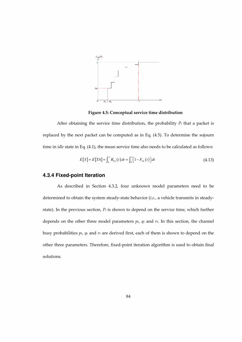
84

Figure 4.5: Conceptual service time distribution

After obtaining the service time distribution, the probability Pf that a packet is

replaced by the next packet can be computed as in Eq. (4.5). To determine the sojourn

time in idle state in Eq. (4.1), the mean service time also needs to be calculated as follows:

[ ] [ ] ( ) ( )0 0

1TA TA

E S E TA R t dt F t dtτ∞

= = = − ∫ ∫ (4.13)

4.3.4 Fixed-point Iteration

As described in Section 4.3.2, four unknown model parameters need to be

determined to obtain the system steady-state behavior (i.e., a vehicle transmits in steady-

state). In the previous section, Pf is shown to depend on the service time, which further

depends on the other three model parameters pb, qb and rb. In this section, the channel

busy probabilities pb, qb and rb are derived first, each of them is shown to depend on the

other three parameters. Therefore, fixed-point iteration algorithm is used to obtain final

solutions.

85

Let Ncs denote the average number of vehicles in the carrier sensing range of the



2cs tr

N N Rβ= = (4.14)


4 2ph cs

N R N Rβ β= − = (4.15)

From the tagged vehicle’s point of view, pb is the probability that it senses

channel busy during one backoff time slot. Through the SMP model in Fig. 4.3, we know

that state I∈ {0,1,…,W-1} stands for the backoff time slot. Furthermore, before the system

enters one of these backoff time slots, the channel has been idle for either one time slot

or DIFS time duration, which can be easily seen from the input transitions and states for

state I. Therefore, to be more precise, pb stands for the probability that the channel

becomes busy (i.e., goes from idle to busy) during one backoff time slot of the tagged

vehicle. The probability that a vehicle starts to transmit during one time slot is given by

π1, which can be computed from Eq. (4.3), because the sojourn time in state 1 is one time

slot. Furthermore, the channel becomes busy if there is at least one neighbor (i.e., a

vehicle in the transmission range of the tagged vehicle) that starts to transmit in a

backoff time slot of the tagged vehicle. Thus, we have:

( )( )

1

1

0

1 1 1!

tr tr

i

i tr N N

b

i

Np e e

i

ππ∞

− − ⋅

=

= − − = −∑ (4.16)

86

Next, qb denotes the probability that the channel is detected busy by the tagged

vehicle in DIFS duration. Different from pb derivation, the channel does not necessarily

become busy during DIFS duration. In other words, the channel can becomes busy

before DIFS duration, and only been detected busy during this DIFS duration. This is

because the tagged vehicle is in state idle while waiting for a packet being generated and

then it enters state CS1 to sense the channel for DIFS duration, which implies that the

channel could have become busy before such DIFS sensing time. As long as the channel

busy status is captured by the DIFS channel sensing time, with probability qb, the vehicle

will enter state DCS to defer transmission. Therefore, to be more precise, qb stands for the

probability that channel busy status is captured by DIFS duration. We can first define QTX

to be the probability that a neighbor’s transmission is captured in the DIFS duration by

the tagged vehicle, hence:

1

1

TX TX

A DIFSQ

Aπ

+= (4.17)

Therefore, qb is given by:

( )( )

0

1 1 1!

tr tr TX

i

i tr N N Q

b TX

i

Nq Q e e

i

∞− − ⋅

=

= − − = −∑ (4.18)

Next we derive an expression for rb. In Section 4.3.2, rb presents the probability

that the following phenomena occurs: the tagged vehicle (vehicle B) waits for the current

packet (from vehicle A) in the channel to finish transmission, and then sense the channel

for DIFS time, which captures the transmission from another vehicle (vehicle C) and

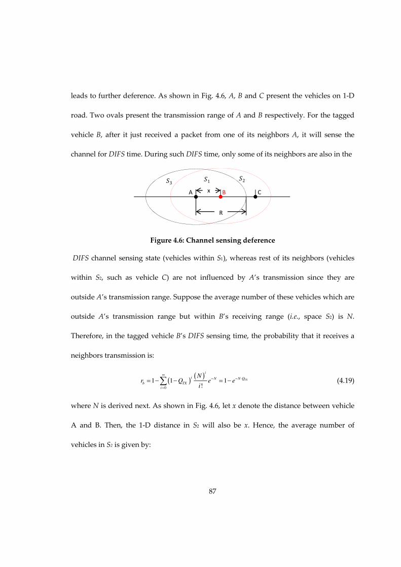
87

leads to further deference. As shown in Fig. 4.6, A, B and C present the vehicles on 1-D

road. Two ovals present the transmission range of A and B respectively. For the tagged

vehicle B, after it just received a packet from one of its neighbors A, it will sense the

channel for DIFS time. During such DIFS time, only some of its neighbors are also in the

x

R

A B C

�1 �2 �3

Figure 4.6: Channel sensing deference

DIFS channel sensing state (vehicles within S1), whereas rest of its neighbors (vehicles

within S2, such as vehicle C) are not influenced by A’s transmission since they are

outside A’s transmission range. Suppose the average number of these vehicles which are

outside A’s transmission range but within B’s receiving range (i.e., space S2) is N.

Therefore, in the tagged vehicle B’s DIFS sensing time, the probability that it receives a

neighbors transmission is:

( )( )

0

1 1 1!

TX

i

i N QN

b TX

i

Nr Q e e

i

∞− ⋅−

=

= − − = −∑ (4.19)

where N is derived next. As shown in Fig. 4.6, let x denote the distance between vehicle

A and B. Then, the 1-D distance in S2 will also be x. Hence, the average number of

vehicles in S2 is given by:

88

0

1

2 4

Rtr

NRN x dx

R

ββ= ⋅ = =∫ (4.20)

Combining Eqs. (4.17)(4.19)(4.20), we obtain rb.

From the above analysis, we know that the four parameters Pf, pb, qb and rb are

interdependent. Hence, the fixed-point iteration algorithm is utilized and outlined as

follows to obtain the final converged solutions:

Step 1: Initialize Pf=0,pb=0,qb=0,rb=0.

Step 2: With Pf, pb, qb, rb, calculate new Pf, pb, qb, rb according to Eqs. (4.5)(4.16)(4.18)(4.19).

Step 3: If Pf, pb, qb, rb converge with the previous values, then stop the algorithm;

otherwise, go to step 2 with the updated Pf, pb, qb, rb.

Once the parameters Pf, pb, qb, rb are determined using the above algorithm, they are used

for the performance-indices computation in the next section.

4.4 Performance Indices

4.4.1 MAC-level Performance Metrics

4.4.1.1 Mean Transmission Delay

One of the most important performance indices is the mean transmission delay

of the beacon message. Different from the mean service time that takes into account all

of the packets generated, the mean transmission delay only accounts for the packets

transmitted and exclude those that have been replaced. Let E[D] be the mean

transmission delay, that is also the mean service time of transmitted packets. Since the

89

service time for the packet that has been replaced is τ and the mean service time is given

in Eq. (4.13), we have:

[ ] ( ) [ ]1f f

E S P E D P τ= − ⋅ + ⋅ (4.21)

Therefore, the mean transmission delay is:

[ ][ ]1

f

f

E S PE D

P

τ− ⋅=

− (4.22)

4.4.1.2 Packet Delivery Ratio

The PDR [7] is the probability that all vehicles in the tagged vehicle’s

transmission range successfully receive the broadcast packet from the tagged vehicle.

Using the approach in [52] in Chapter 2, we have:

( ) ( )cs phPDR P N P N= (4.23)

Note that the formulas for P(Ncs) and P(Nph) in [52] in Chapter 2 are adjusted

according to the newly proposed model in this chapter. P(Ncs) can also be interpreted as

the non-concurrent transmission probability, i.e., two packets do not start transmission

in the same time slot. Since the sojourn time in state 1 is one time slot, π1 is equivalent to

the probability that a vehicle starts to transmit in a time slot. Hence, P(Ncs) is given by:

( ) ( )( ) ( ) ( ) 11 1

1

0

11

!

cs cs

i

i N Ncs

cs

i

NP N e e

i

ππ∞

− − − −

=

−= − =∑ (4.24)

The event that a transmission from hidden terminals collides with the tagged

vehicle’s transmission only happens when hidden terminals start to transmit during the

vulnerable period of duration 2·A1 [7]. Therefore, the probability that a vehicle starts to

90

transmit during the vulnerable period of hidden terminal transmissions [7] is 2·πTX, and

hence:

( ) ( )( ) 2

0

1 2!

ph ph TX

i

phi N N

ph TX

i

NP N e e

i

ππ

∞− − ⋅ ⋅

=

= − ⋅ =∑ (4.25)

4.4.1.3 Packet Reception Ratio



investigated at the moment that the packet is sent out [7]. Using an approach similar to

that presented in [52] in Chapter 2, we adjusted and simplified the formulas according to

the new model. Hence:

cc htPRR PRR PRR= (4.26)

where the impact of the concurrent transmission is:

1

11 2

1

(1 )R

R

cc cc cc

ePRR PRR PRR e

R

β πβ π

β π

−−= ⋅ = − (4.27)

and the impact of the hidden terminal is:

( )(2 )11 csC R lh cs

ht

R NF l RPRR e

R R RC

β

β− −− −

= = + − (4.28)

with C=2β· πTX.

4.4.1.4 Normalized Channel Throughput

The normalized channel throughput is the ratio of the time used for successful

transmitted packets and the entire time. From a channel’s perspective, during one packet

91

generation interval τ, Ntr packets are generated in total for all vehicles sensing this

channel, one packet from each vehicle. Hence, the normalized channel throughput can

be easily computed as:

trNS PDR PL

τ= ⋅ ⋅ (4.29)

4.4.2 Application-level Performance Metrics

Besides MAC-level metrics, application-level performance metrics are also

important to capture the performance of broadcast-based safety applications.

Furthermore, the QoS requirements are typically expressed in terms of application-level

performance metrics. Therefore, derivation of the application-level performance metrics

is essential for QoS assessment of safety applications. To derive the application-level

performance metrics, the evaluation of point-to-point reception probability needs to be

conducted through coverage area computation for the impact of hidden terminal

problem and concurrent transmissions. Therefore, the node reception probability is first

computed, based on which the application-level performance metrics including T-

window reliability, application-level delay, awareness probability and average number

of invisible neighbors are derived.

4.4.2.1 Node Reception Probability

Given a transmitting node O placed at the origin (see Fig. 4.7), U is one of the

receivers within transmission range R of node O. U is placed on 1-D line with certain

distance to O, which is denoted as x (0<x<R). The probability that the node U receives

92

the broadcast message from the tagged node O successfully is the node reception

probability (NRP) at distance x, which is denoted as Ps(x).

Tagged node

R R

Hidden terminalsHidden terminals X

V U

Transmission range

of tagged node

• • • • • • • • • • • • •

R R

O

R-X

z

Figure 4.7: Node reception probability computation

There are two factors affecting the node reception probability: hidden terminal

problems, collisions due to concurrent packet transmissions:

a. Impact of Hidden terminals

Based on the SMP model and its solution, we have the probability that node U’s

reception of the broadcast message from node O is free from the hidden terminals:

x

i

xi

i

TXHTXee

i

xxP

βπββπ 2

0 !

)()21()(

−∞

=

−∑ =−= (4.30)

b. Impact of concurrent collisions

In addition to collisions caused by the hidden nodes, transmissions from nodes

within interference range from the tagged node in the meantime at which the tagged

node transmits may also cause collisions. When the tagged node transmits in a slot time,

collisions will take place if any node in the interference range of the tagged node

transmits in the slot.

Given that as both O and U sense the channel idle, O will transmit within the

duration of a slot. In order to prevent interference due to concurrent collisions to U’s

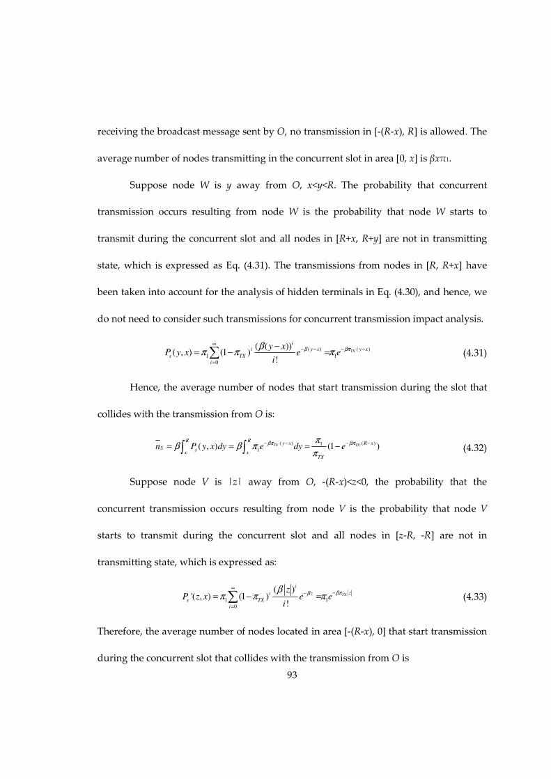
93

receiving the broadcast message sent by O, no transmission in [-(R-x), R] is allowed. The

average number of nodes transmitting in the concurrent slot in area [0, x] is βxπ1.

Suppose node W is y away from O, x<y<R. The probability that concurrent

transmission occurs resulting from node W is the probability that node W starts to

transmit during the concurrent slot and all nodes in [R+x, R+y] are not in transmitting

state, which is expressed as Eq. (4.31). The transmissions from nodes in [R, R+x] have

been taken into account for the analysis of hidden terminals in Eq. (4.30), and hence, we

do not need to consider such transmissions for concurrent transmission impact analysis.

( )( )

1 1

0

( ( ))( , ) (1 )

!TX

iy xi y x

s TX

i

y xP y x e e

i

βπββπ π π

∞− −− −

=

−= − =∑ (4.31)

Hence, the average number of nodes that start transmission during the slot that

collides with the transmission from O is:

( ) ( )1

1( , ) (1 )TX TX

R Ry x R x

S sx x

TX

n P y x dy e dy eβπ βππ

β β ππ

− − − −= = = −∫ ∫ (4.32)

Suppose node V is |z| away from O, -(R-x)<z<0, the probability that the

concurrent transmission occurs resulting from node V is the probability that node V

starts to transmit during the concurrent slot and all nodes in [z-R, -R] are not in

transmitting state, which is expressed as:

1 1

0

( )'( , ) (1 )

!

TX

i

zi z

s TX

i

zP z x e e

i

βπββπ π π

∞−−

=

= − =∑ (4.33)

Therefore, the average number of nodes located in area [-(R-x), 0] that start transmission

during the concurrent slot that collides with the transmission from O is

94

( ) ( )

0 0

1

' ( )1

10

'( , )

' (1 )

TX

TX TX

zT s

R x R x

R xz R x

TX

n P z x dz e dz

e dz e

βπ

βπ βπ

β β π

πβ π

π

−

− − − −

−− − −

= =

= = −

∫ ∫

∫ (4.34)

Hence, the total average number of nodes that may transmit concurrently is:

1πβxnnn Ts ++=∑ (4.35)

Therefore, given Poisson node distribution, the probability that no nodes within

the reception range of U start transmission during the slot that collides with the

transmission from O is:

)exp()exp(!0

)()(

0

∑∑∑

−=−= nnn

xPcon

(4.36)

Taking hidden terminal and possible packet collisions, the node reception

probability that the node U receives the broadcast message from the tagged node O is:

)()()( xPxPxP conHs = (4.37)

4.4.2.2 T-window Reliability

Application-level T-window reliability is defined in [53] as the probability of

successfully receiving at least one packet out of multiple packets from a broadcast

vehicle at distance x, within a given time T (referred to as application tolerance

window):

τ

T

sapp xPTxP ))(1(1),( −−=

(4.38)

where τ is the beacon generation interval and Ps(x) is the node reception probability

given in Eq. (4.37).

95

4.4.2.3 Application-level Delay

Application-level latency [53] TD is the duration between the time when a

broadcast packet is generated at application layer of transmitting vehicle and the time at

which the first successful packet is received by the application layer of receiving vehicle.

Suppose the distance between the transmitting vehicle and the receiving vehicle is x, the

average application-level delay is given by:

( ) [ ] 1

1

1( 1) [ ] ( )(1 ( )) [ ] 1

( )D

i

T s s

i s

E x i E D P x P x E DP x

τ τ∞

−

=

= − + − = + −

∑ (4.39)

where E[D] is the mean transmission delay of the beacon message, which is given in Eq.

(4.22).

4.4.2.4 Awareness Probability

The awareness probability [54] is the probability of successfully receiving at least

n packets in the tolerance time window T.

( , ) ( ) (1 ( ))

T

Tk

k

A s s

k n

T

P x n P x P x

k

τττ

−

=

= −

∑ (4.40)

where x is the distance between the sender and receiver. It is noted that the awareness

probability PA(x, n) becomes the application-level T-window Reliability Papp(x, T) as n is

equal to 1.

96

4.4.2.5 Average Number of Invisible Neighbors

Region of interest (ROI) has been proposed in [53] to present the size of the

geographical region covered by entities participating in an application. For a safety

application to work properly, a vehicle needs to be aware of the neighbors’ status within

ROI. Different applications may have different ROI. The invisible neighbor problem is

defined in [55]: if vehicle A has not received any broadcast packet from vehicle B for a

certain time interval, vehicle B is an invisible neighbor of A. Therefore, under the

concept of ROI, the number of invisible neighbors needs to be under a certain constraint

to satisfy the QoS of an application. We adopt this concept and newly define another

application-level performance metric: average number of invisible neighbors within

range x from the receiver after a tolerant time window T.

0 0

1( ) 2 1 ( , ) 2 2 ( , )

x x

invisible app appN x x P s T ds x P s T ds

xβ β β

= − ⋅ = −

∫ ∫ (4.41)

4.5 Numerical Results

Matlab is used for the computation of analytic models and simulations. The first

subsection describes the simulation procedure. The second subsection compares the

analytic results with the simulations, which show the high accuracy of our

decomposition-based analytic approximation. The last subsection compares the model in

[52] (Poisson arrival with infinite queue) and the model in [51] with the new proposed

model (periodic arrival with packet replacement strategy).

97

4.5.1 Numerical Results for MAC-level Performance Metrics

4.5.1.1 Simulation Description

Discrete-event simulation is conducted in Matlab to assess the approximation

error in the decomposition and fixed-point iteration used in solving the analytic model.

Different from the decomposition method used for the analytic model, the simulation

process simulates the overall system behavior of the GSMP model. To better illustrate

the simulation procedure, a brief simulation flow chart is presented in Fig. 4.8. Note that

this flow chart is drawn from the whole system’s perspective, whereas each individual

vehicle’s behavior is consistent with the operation flow in Fig. 2.1. In Fig. 4.8, neighbors

of the transmitting vehicle refer to the vehicles within the transmitting vehicle’s

transmission range. Possible backoff behavior of the neighbors is considered while

deferring or resetting their next event time. This simulation procedure is performed

multiple times based on independent replications, from which confidence intervals of

the output measures are computed.

Figure 4.8: Simulation flow chart

98

4.5.1.2 Analytic Vs. Simulation Results

The same typical DSRC parameter settings as that in Table 3.1 in [52] are used for

the proposed model. The numerical results from the analytic solution including mean

transmission delay, PDR, PRR and normalized throughput are plotted in Figs. 4.9-4.12

respectively, vs. the vehicle density β (# vehicles per meter), data rate Rd (Mbps), packet

generation interval τ (second) and packet length PL (byte).

We conducted 30 runs of simulation and each run last 5 seconds. Due to the

Central Limit Theorem, normal distribution is assumed to compute confidence intervals

for the population means of the output measures. Eq. (4.42) shows the 100(1-α)%

confidence interval for population mean x, where x stands for the sample mean, σ for

sample variance, n for sample size (i.e., number of simulation runs) and z for critical

value of normal distribution.

/2 /2x z x x z

n nα α

σ σ− ⋅ ≤ ≤ + ⋅ (4.42)

The simulation results for 95% confidence interval are also illustrated in Figs. 4.9-

4.12 to compare with analytic-numerical results. The good match of the analytic and the

simulation results verifies the accuracy of our proposed model. The packet replacement

probability Pf is extremely low from our numerical analysis resulting from the fact that

packet transmission delay is much smaller than the packet generation interval as shown

in Fig. 4.9. Figs. 4.9-4.11 show that mean transmission delay, PDRs and PRRs benefit

from high data rate and short packet length. Furthermore, PDRs are less than PRRs

99

given the same network parameters. Fig. 4.12 shows that normalized channel

throughput increases as vehicle density increases resulting from more severe channel

contentions. It may become saturated due to more severe packet collisions.

0.02 0.04 0.06 0.08 0.1 0.12 0.14 0.16 0.18 0.20

0.5

1

1.5

2

2.5

3

3.5

4

4.5

5x 10

-4

density(#vehicles/m)

me

an d

ela

y (

secon

ds)

Rd=12,tau=0.5,PL=200,Analytic




Figure 4.9: Mean transmission delay

0.02 0.04 0.06 0.08 0.1 0.12 0.14 0.16 0.18 0.20

0.1

0.2

0.3

0.4

0.5

0.6

0.7

0.8

0.9

1


Packet

Deliv

ery

Ratio





Figure 4.10: Packet delivery ratio

0.02 0.04 0.06 0.08 0.1 0.12 0.14 0.16 0.18 0.20.5

0.55

0.6

0.65

0.7

0.75

0.8

0.85

0.9

0.95

1


Packet

Reception R

atio





Figure 4.11: Packet reception ratio

0.02 0.04 0.06 0.08 0.1 0.12 0.14 0.16 0.18 0.20

0.02

0.04

0.06

0.08

0.1

0.12


Norm

aliz

ed T

hro

ughput





Figure 4.12: Normalized channel

throughput

4.5.1.3 Compare with Previous Models

In this section, the model in [52] and the model in [51] are compared with our

proposed model. These three models are comparable since all of them concentrate on

100

MAC layer behavior of safety message transmissions. However, the model in [52],

denoted as model 1, assumes Poisson packet arrivals and that each vehicle has an

infinite queue to store generated packets, which may be unrealistic for beacon messages.

The proposed model, denoted as model 2, relaxes these assumptions and focuses on

periodic message generation and no queue scenario (i.e., out-dated message is replaced

by the new message), which is more practical. Bastani’s model proposed in [51]

accounted for the periodic nature of beacon message generations and new message

canceling out old message phenomena. However, their model does not accurately

capture the periodic beacon message generation since it separates the periodic message

generation from the message channel contention and transmission behavior, although

these behaviors are closely correlated. Since the output measures computed in [51] are

different from those we calculated in this chapter, Bastani’s model is slightly modified,

denoted as model 3, to obtain PDR for comparison. Eq. (11) in [51] for probability of

successful transmission is modified to compute packet delivery ratio (PDR) of beacon

message only as follows:

( )1

(1 )1

bh

tr ph bs

TN N

b p T pPDR στ− + ⋅

⋅ + −= − (4.43)

where

( )2

; 1 1 ; 2 ; /1 2 /

trNb b b b b

h s s d Hp T T T PL R TW

τ τ δτ σ

= = − − = = + ++ +

(4.44)

Figs. 4.13-4.15 present the analytic-numerical results comparison of these three models.

Notice that packet generation rate λ in model 1 is set to be equivalent to the reciprocal of

101

the packet generation interval τ in model 2 and model 3. The results show that the mean

transmission delay obtained from model 2 is slightly higher than that from model 1,

whereas the PDR and PRR are slightly lower than that from model 1. Taking into

consideration the variations in the simulations results (i.e., 95% confidence intervals) in

Figs. 4.9-4.11, we can conclude that model 1 leads to similar results with model 2. In

other words, Poisson arrival with infinite queue scenario can be used to approximate the

periodic beacon message generation without any queue case. Such phenomena may

result from the fact that the packet generation interval is much larger than the packet

transmission delay, which further implies that a packet is out-dated and replaced by the

next packet with a very low probability. Therefore, queue length does not have

significant influence on packet transmissions. Fig. 4.14 also shows that PDR obtained

from model 3 has a good match with model 1 and model 2 when the beacon message

generation interval is longer. However, when the beacon message is generated more

frequently, model 3 has much higher PDR than model 1 and model 2. Compared with

the simulation results in Fig. 4.10, we conclude that model 3 is not as accurate as model 2

proposed in this chapter. The possible reason is already stated earlier.

102

0.02 0.04 0.06 0.08 0.1 0.12 0.14 0.16 0.18 0.20

0.5

1

1.5

2

2.5

3

3.5

4

4.5

5x 10

-4


Mean D

ela

y (

second)

Rd=12,lam=2,PL=200,model1


Rd=12,tau=0.5,PL=200,model2


Figure 4.13: Comparison of mean delay

0.02 0.04 0.06 0.08 0.1 0.12 0.14 0.16 0.18 0.2

0.6

0.65

0.7

0.75

0.8

0.85

0.9

0.95

1


PD

R







Figure 4.14: Comparison of PDR

0.02 0.04 0.06 0.08 0.1 0.12 0.14 0.16 0.18 0.20.6

0.65

0.7

0.75

0.8

0.85

0.9

0.95

1


PR

R





Figure 4.15: Comparison of PRR

4.5.2 Analytic-Numerical Results for Application-level Performance Metrics

4.5.2.1 Analytic-numerical Results for Fixed Network Parameters

Table 4.1: Network parameter settings


Transmission range R 500 m Packet length PL 400 bytes

Time window T 1 s Beacon message interval τ 0.1 s

Data rate Rd 24 Mbps Vehicle density β 0.1 vehicles/m

103

In this section, the application-level performance metrics are evaluated for a

given network parameter settings as shown in Table 4.1.

Fig. 4.16 shows that NRP decreases linearly with the distance from the sender.

The awareness probability also decreases with the distance to the sender. Note that the

Application-level T-window Reliability is equivalent to the awareness probability with

packet requirement n=1. The application with stricter packets requirements has lower

awareness probability. During the time window T=1s, there are 10 beacon packets sent

out from the sender since the beacon message interval is 0.1s. If the packet requirement

is less than or equals to 5 packets, the awareness obtained is larger than 99%, which can

ensure the application works appropriate even though the NRP in the network layer is

not very high. Otherwise, if the packet requirement is larger than 5 among 10 packets

transmitted within 1 second, the application layer awareness probability may be even

lower than the NRP in the network layer as seen from PA(n=8) case. Hence, for some

applications that require more than 5 packets within T=1s, the reliability requirement

may not be met.

104

0 50 100 150 200 250 300 350 400 450 5000.7

0.75

0.8

0.85

0.9

0.95

1

Distance (m)

Pro

babili

ty

NRP

PA(n=1)

PA(n=5)

PA(n=6)

PA(n=7)

PA(n=8)

Figure 4.16: Node reception probability (NRP) and awareness probability (PA) with

different packet requirement n

0 50 100 150 200 250 300 350 400 450 5000

0.005

0.01

0.015

0.02

0.025

Distance (m)

Applic

ation

-levle

Dela

y (

secon

d)

Figure 4.17: Application-level delay

0 50 100 150 200 250 300 350 400 450 5000

0.5

1

1.5

2

2.5

3

3.5

4x 10

-7

Distance (m)

Avera

ge N

o.

of

Invis

ible

Neig

hbors

Figure 4.18: Average no. of invisible

neighbors

Fig. 4.17 shows that the application-level delay increases almost linearly with the

distance. Furthermore, compared to the MAC-level transmission delay in Fig. 4.9, the

application-level delay is much higher, especially when the distance between the sender

and receiver is large. Such phenomena results from the fact that NRP decreases linearly

according to the distance. Fig. 4.18 shows that the number of invisible neighbors

105

increases fast when the distance exceeds 300m. However, the number of invisible

neighbors is quite small (in the order of 1E-6), which means that the receiver can receive

at least one packet from almost every neighbor within time window T=1s and hence all

neighbors are visible to the receiver.

4.5.2.2 Analytic-numerical Results for Different Network Parameters

In order to evaluate the influences of different network parameters such as data

rate, beacon message interval and packet length on the application-level metrics, we

vary three input parameter value in Table 4.1 and analyze the output measures as

shown in Figs. 4.19-4.22. The legend represents the data rate Rd (Mbps), beacon message

interval τ (s) and data length PL (bytes), respectively.

Fig. 4.19 and Fig. 4.20 show that increasing the data rate helps increasing NRP

and awareness probability (more obvious when the distance to the sender is large).

Another important observation is that decreasing the beacon message interval (i.e.,

messages are sent more frequently) will decrease the NRP, but increase awareness

probability. This implies that even though more collisions occur in the MAC layer

resulting from higher beacon message generation rate, we may still obtain satisfied QoS

in the application layer. Furthermore, increasing the packet length leads to decreasing

NRP and decreasing awareness probability. Therefore, we can improve the awareness

probability by increasing the data rate, decreasing the data length or decreasing the

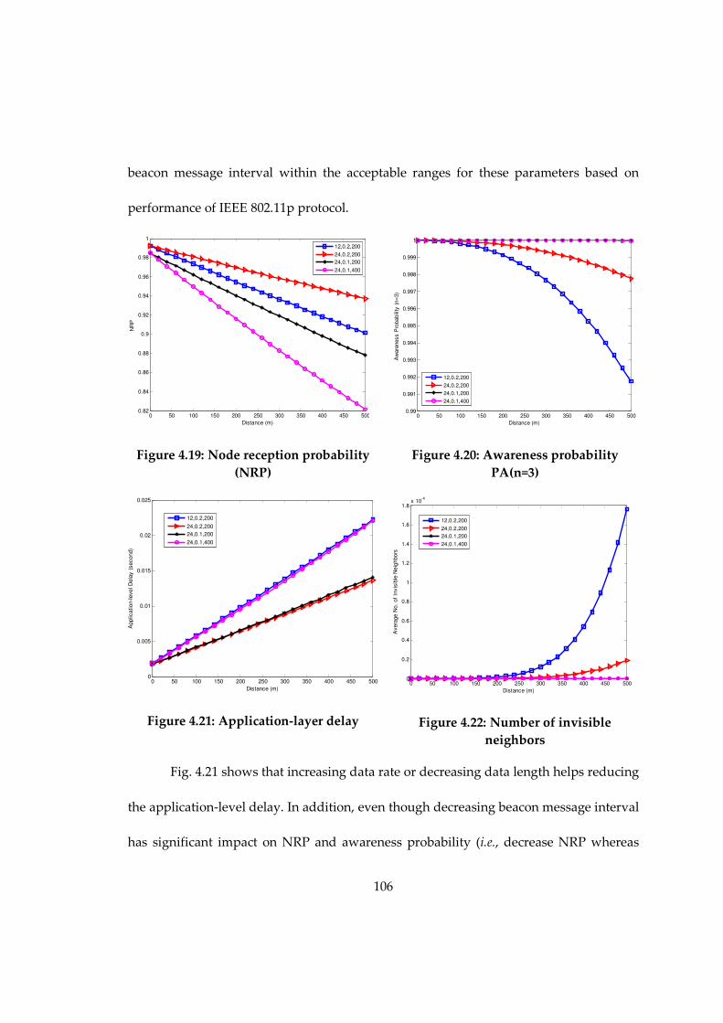
106

beacon message interval within the acceptable ranges for these parameters based on

performance of IEEE 802.11p protocol.

0 50 100 150 200 250 300 350 400 450 5000.82

0.84

0.86

0.88

0.9

0.92

0.94

0.96

0.98

1

Distance (m)

NR

P

12,0.2,200

24,0.2,200

24,0.1,200

24,0.1,400

Figure 4.19: Node reception probability

(NRP)

0 50 100 150 200 250 300 350 400 450 5000.99

0.991

0.992

0.993

0.994

0.995

0.996

0.997

0.998

0.999

1

Distance (m)

Aw

are

ness P

robabili

ty (

n=

3)

12,0.2,200

24,0.2,200

24,0.1,200

24,0.1,400

Figure 4.20: Awareness probability

PA(n=3)

0 50 100 150 200 250 300 350 400 450 5000

0.005

0.01

0.015

0.02

0.025

Distance (m)

Applic

ation-level D

ela

y (

second)

12,0.2,200

24,0.2,200

24,0.1,200

24,0.1,400

Figure 4.21: Application-layer delay

0 50 100 150 200 250 300 350 400 450 5000

0.2

0.4

0.6

0.8

1

1.2

1.4

1.6

1.8x 10

-4

Distance (m)

Avera

ge

No.

of

Invis

ible

Ne

ighbors

12,0.2,200

24,0.2,200

24,0.1,200

24,0.1,400

Figure 4.22: Number of invisible

neighbors

Fig. 4.21 shows that increasing data rate or decreasing data length helps reducing

the application-level delay. In addition, even though decreasing beacon message interval

has significant impact on NRP and awareness probability (i.e., decrease NRP whereas

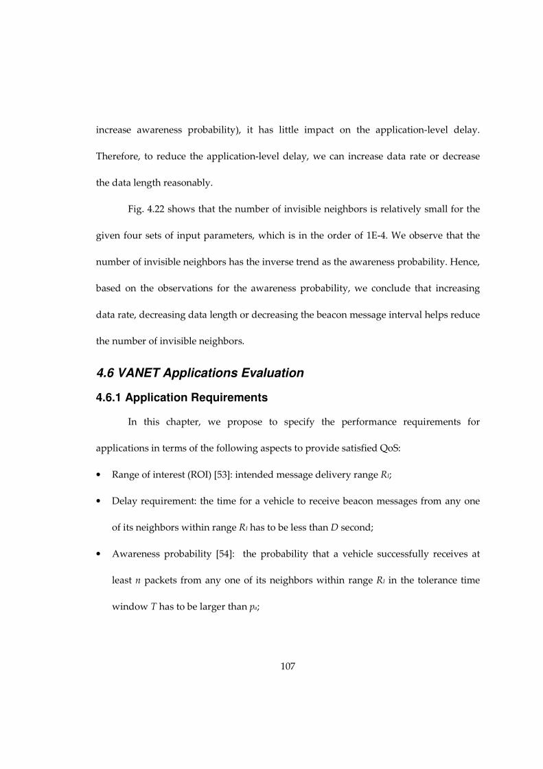
107

increase awareness probability), it has little impact on the application-level delay.

Therefore, to reduce the application-level delay, we can increase data rate or decrease

the data length reasonably.

Fig. 4.22 shows that the number of invisible neighbors is relatively small for the

given four sets of input parameters, which is in the order of 1E-4. We observe that the

number of invisible neighbors has the inverse trend as the awareness probability. Hence,

based on the observations for the awareness probability, we conclude that increasing

data rate, decreasing data length or decreasing the beacon message interval helps reduce

the number of invisible neighbors.

4.6 VANET Applications Evaluation

4.6.1 Application Requirements

In this chapter, we propose to specify the performance requirements for

applications in terms of the following aspects to provide satisfied QoS:

• Range of interest (ROI) [53]: intended message delivery range RI;

• Delay requirement: the time for a vehicle to receive beacon messages from any one

of its neighbors within range RI has to be less than D second;

• Awareness probability [54]: the probability that a vehicle successfully receives at

least n packets from any one of its neighbors within range RI in the tolerance time

window T has to be larger than pa;

108

• Average number of invisible neighbors [55]: the average number of invisible

neighbors within range RI in tolerance time window T has to be less than N;

Given the above application-level performance metrics, our proposed analytic models

can be used to evaluate whether the given network parameters can satisfy the QoS

requirement or not for an application. In addition, we can provide insights to tune the

network parameters to meet the application requirements.

4.6.2 Case Studies for VANET Applications

Vehicles are able to track surrounding vehicles’ status by their periodically

broadcasted beacon messages containing position, velocity and acceleration. Many

safety applications judge the risk based on such information and provide corresponding

warnings to the driver to prevent potential accidents. In this section, three typical safety

applications [58] are analyzed.

4.6.2.1 Emergency Vehicle Warning

Vehicles can receive route information of emergency vehicles (e.g., police cars,

ambulances, fire trucks etc.) from the beacon messages received. Hence, based on such

information, emergency vehicle warning application [59] enables drivers to be aware of

the emergency vehicle and take appropriate actions to reduce accidents and save time.

Some reasonable assumptions are made for the performance requirements of the

emergency vehicle warning application: The ROI is 500m [60]; Delay requirement is

1000ms [60]; Awareness probability that a vehicle successfully receives at least 1 packet

109

in the tolerance time window T=1s is larger than 99.9%; Average number of invisible

neighbors is less than 1.

0 50 100 150 200 250 300 350 400 450 5000.93

0.94

0.95

0.96

0.97

0.98

0.99

1

Distance (m)

NR

P

0 50 100 150 200 250 300 350 400 450 500

0.9999990

0.9999991

0.9999992

0.9999993

0.9999994

0.9999995

0.9999996

0.9999997

0.9999998

0.9999999

1

Distance (m)

Aw

are

ness

Pro

ba

bili

ty

0 50 100 150 200 250 300 350 400 450 5000

0.002

0.004

0.006

0.008

0.01

0.012

0.014

Distance (m)

Applic

ation-level D

ela

y (

second)

0 50 100 150 200 250 300 350 400 450 5000

0.2

0.4

0.6

0.8

1

1.2

1.4

1.6

1.8

2x 10

-5

Distance (m)

Avera

ge N

o.

of

Invis

ible

Neig

hbors

Figure 4.23: Emergency vehicle warning application-level metrics with parameters

Rd=24, τ=0.2, PL=200

Fig. 4.23 shows that the application-level delay, awareness probability and

average number of invisible neighbors requirement can all be satisfied with given input

parameters Rd=24Mbps, τ=0.2s, PL=200bytes.

110

4.6.2.2 Slow Vehicle Indication

Slow vehicle indication application [58] is able to provide alerts to the driver

about potential hazard if a slow vehicle is detected based on the beacon messages

received. For the slow vehicle indication application to work properly, the vehicle has to

receive beacon messages from the slow vehicle timely and reliably. This application may

have stricter awareness requirements than the emergency vehicle warning application.

0 10 20 30 40 50 60 70 80 90 1000.98

0.985

0.99

0.995

Distance (m)

NR

P

0 10 20 30 40 50 60 70 80 90 100

0.99993

0.99994

0.99995

0.99996

0.99997

0.99998

0.99999

1

Distance (m)

Aw

are

ness P

robabili

ty

0 10 20 30 40 50 60 70 80 90 1001.5

2

2.5

3

3.5

4

4.5

5x 10

-3

Distance (m)

Applic

ation-level D

ela

y (

second)

0 10 20 30 40 50 60 70 80 90 100

0

0.2

0.4

0.6

0.8

1

1.2

1.4

1.6x 10

-8

Distance (m)

Ave

rage N

o.

of

Inv

isib

le N

eig

hbors

Figure 4.24: Slow vehicle indication application-level metrics with parameters Rd=24,

τ=0.2, PL=200

111

The performance requirement assumptions can be made as follows: The ROI is 100m;

Delay requirement is 50ms; Awareness probability that a vehicle successfully receives at

least 3 out of 5 packets in the tolerance time window T=1s is larger than 99.9%; Average

number of invisible neighbors is less than 1.

Fig. 3.24 shows that application-level delay, awareness probability and average

number of invisible neighbors requirement can all be satisfied with given input

parameters Rd =24Mbps, τ=0.2s, PL=200bytes.

4.6.2.3 Rear-end Collision Warning

Rear-end collision warning application should have stricter awareness

requirements than the previous two applications since it is more critical for safety.

Therefore, we suggest the performance requirements to be: The ROI is 50m; Delay

requirement is 20ms [60]; Awareness probability that a vehicle successfully receives 4

out of 5 packets in the tolerance time window T=1s is larger than 99.9%; Average

number of invisible neighbors is less than 1.

0 10 20 30 40 50 600.985

0.986

0.987

0.988

0.989

0.99

0.991

0.992

0.993

0.994

Distance (m)

NR

P

0 10 20 30 40 50 60

0.9978

0.998

0.9982

0.9984

0.9986

0.9988

0.999

0.9992

0.9994

0.9996

Distance (m)

Aw

are

ness P

robabili

ty

112

0 10 20 30 40 50 601.6

1.8

2

2.2

2.4

2.6

2.8

3

3.2x 10

-3

Distance (m)

Applic

ation-leve

l D

ela

y (

second)

0 10 20 30 40 50 60

0

0.5

1

1.5

2

2.5

3x 10

-9

Distance (m)

Avera

ge N

o.

of

Invis

ible

Neig

hbors

Figure 4.25: Rear-end collision avoidance application layer metrics with parameters

Rd=24, τ=0.2, PL=200

Fig. 3.25 shows that the application-level delay and average number of invisible

neighbors can satisfy the requirement given the input parameters. However, the

awareness probability is lower than 99.9% when the distance to the sender is larger than

20m. Therefore, the rear-end collision avoidance application cannot provide the

satisfactory QoS for the given input parameters. To meet the application requirement,

based on the conclusions obtained in Section 4.5.2.2, we can improve the awareness

probability by increasing the data rate, decreasing the data length or decreasing the

beacon message interval.

4.7 Conclusions

In this chapter, an analytic model is developed to characterize the periodic

beacon message dissemination in DSRC for highway safety communications. Instead of

assuming Poisson arrivals and infinite queue as in most of the literature, the periodic

113

packet generation and out-dated information replacement are taken into consideration

in the new proposed model. Important MAC-level performance indices such as the

mean transmission delay, PDR, PRR and normalized channel utilization are analytically

derived and computed. Detail simulations for the overall system in the MAC layer are

conducted to verify the accuracy of the decomposed model. The model is also compared

with previous model that assumed Poisson arrival and infinite queue and Bastani’s

model.

Besides MAC-level performance evaluation, application-level performance

metrics including T-window reliability, application-level delay, awareness probability

and average number of invisible neighbors are analytically derived based on the node

reception probability. The analytic-numerical results are evaluated for application-level

performance metrics under various network parameters. Such analysis can be very

useful for tuning network parameters in order to obtain satisfied QoS for many safety

applications. Three typical safety applications including emergency vehicle warning,

slow vehicle indication and rear-end collision warning are assessed to check whether

their performance requirements can be met for a given network parameter setting.

In the next chapter, we will take into account the channel switching behavior [26]

between the control channel and service channels, where the control channel is used for

beacon message and service channels are used for other types of messages. Furthermore,

the assumptions in Section 4.2 will also be relaxed to reflect real world traffic scenarios.

114

For example, the MAC layer and application layer performance metrics will be analyzed

incorporating fading channel. In addition to 1-D highway scenarios, 2-D models are also

developed in Chapter 8.

115

5. Multiple Types of Services Evaluation

5.1 Motivation

According to the updated version of the DSRC standard [11], the DSRC physical

layer follows the same frame structure, modulation scheme and training sequences

specified by IEEE 802.11a physical layer standard with minor changes; MAC layer of the

DSRC is equivalent to the Enhanced Distribution Coordination Access (EDCA) 802.11e

that has four different access classes (ACs).

In the literature, unicast for IEEE 802.11 has been extensively investigated.

Bianchi [27] proposed a simple yet accurate discrete-time Markov chain (DTMC) model

to evaluate the MAC-layer performance of unicast mechanism under saturation

conditions. His paper has inspired many other researchers to develop analytic models of

unicast EDCA based on DTMC. The saturation performance for multiple types of

services with priorities using EDCA mechanism has been studied in [81][82][83][84][38].

Many later work [85][86][87][88][89] extended to the unsaturation packet generation

case, which reflects a more practical scenario. However, most previous researches are

based on Bianchi’s DTMC (i.e., per-slot statistics) model [27] and ignore important

aspects of continuous time system behavior leading to approximations. More

specifically, due to the characteristic of such discrete model, backoff counter freezing

behavior cannot be accurately captured. Lee [38] considered such freezing process by

adding sub-Markov chain for multiple services using EDCA. However, the backoff

116

counter freezing time because of the busy medium (i.e., waiting for the packet in the

channel finishing transmission) is still not taken into account. In a recent paper by

Tinnirello and Bianchi [37], an analytic model not based on the per-slot statistics was

proposed through a fixed-point computation of the residual backoff counter distribution

occurring after a generic transmission attempt. However, this is only for the saturation

condition.

Recently, a few analytic models [33][90][91] are proposed to quantify the MAC-

layer performance of multiple types of safety messages using broadcast EDCA over the

control channel in DSRC based VANETs. Gallardo [33] used three DTMC models to

capture the EDCA behavior for three types of messages for the performance evaluation.

However, hidden terminal problem is not considered in this work and no simulation

results are presented to verify the accuracy of the models. Hafeez [90] evaluated the

broadcast performance of two types of safety messages under EDCA taking into

consideration of interferences from hidden terminals. Nevertheless, the analytic model is

also based on DTMC (per-slot analysis) and ignores the continuous time system

behavior. More specifically, the backoff counter freezing process has not been accurately

captured by the DTMC and the post backoff process is also not considered in this work.

In addition, total reliability (i.e., probability of successful reception) for packet

transmission is computed instead of providing separate reliability for each type of

services, which may not lead to comprehensive conclusions. Khabazian [91] proposed an

117

analytic model for the performance of multi-hop message dissemination with two

classes of traffic. However, the detailed backoff process is not considered in the model

and the channel service time is assumed to be exponential distributed, which may lead

to approximations for the transmission delay computation.

In this chapter, we extend the work presented in Chapter 3 [12][52] for one type

of services to three types of services using EDCA mechanism for one-hop direct

broadcast over the control channel. We are interested in whether EDCA mechanism can

provide service differentiations with respect to the performance and reliability. The

generation and service of each type of safety messages in each vehicle is modeled by a

generalized M/G/1 queue, where two classes of service are considered based on Welch’s

method [13]. The overall model is a set of interacting M/G/1 queues, three queues for

each vehicle. The interaction is that the server is shared as it is the contention

medium/channel for the safety message transmissions. To make the model scalable, we

use semi-Markov process (SMP) model to capture the shared server’s behavior for each

service from a single tagged vehicle’s perspective, where the medium/channel

contention and backoff behavior for this type of service and the influence from the same

vehicle and other vehicles are considered. Different from the previous DTMC models

capturing the shared server’s discrete time behavior, this SMP model directly

incorporates the unsaturation condition of the queue in a continuous time fashion. It

interacts with the tagged vehicle’s M/G/1 queue through the fixed-point iteration.

118

The major contributions made in this research are five-fold. First, the proposed

analytic models provide an accurate analysis for different types of broadcast services

over DSRC channel using EDCA mechanism with unsaturated message generation and

hidden terminals in the continuous time. Second, the service time for packets is divided

into two classes (i) for the packet arrivals when the queue is empty; (ii) for the packet

arrivals when the queue is not empty. Based on Welch’s method with two classes of

arrivals in an M/G/1 queue, more accurate results can be obtained. Third, based on the

solution to the interacting SMP model and M/G/1 queuing model, expressions of MAC-

layer performance metrics for DSRC vehicular safety communications are derived.

These metrics include the mean and variance of the transmission delay, packet delivery

ratio (PDR) and packet reception ratio (PRR). The analytic results are verified by

simulations to show the errors in the approximations are small. Fourth, the MAC-layer

performances for EDCA mechanism are evaluated according to various input

parameters. The analysis shows that EDCA provides only latency differentiations but

not reliability. Fifth, the M/G/1 queue is extended to GI/G/1 queue to incorporate more

generalized packet arrival process. Whitt’s method is used to compute the mean and

variance of the waiting time for GI/G/1 queue instead.

This chapter is organized as follows. Section 5.2 briefly describes the system

behavior in IEEE 802.11 MAC layer protocol and lists the assumptions made to produce

a tractable model. Section 5.3 presents the analytic models and the fixed-point iteration.

119

MAC-layer performance indices including mean and variance of the transmission delay,

PDR and PRR are derived in Section 5.4. The analytic and simulation results are

compared in Section 5.5. Section 5.6 presents the extended analytic models to

incorporate generalized distributed packet arrival process using GI/G/1 queue. A case

study is constructed and evaluated in Section 5.7. Conclusions are presented in the last

section.

5.2 System Description and Assumptions

As we know from [1], the DSRC MAC layer adopts IEEE 802.11 MAC layer

specification with minor modifications. In the 802.11 MAC layer protocol [11],

distributed coordination function (DCF) is the primary medium access control technique

for broadcast services. IEEE 802.11p MAC layer utilizes the Enhanced Distribution

Channel Access (EDCA) that has different access classes (ACs) with priorities to ensure

quality of services (QoS). Each class has different backoff window size and Arbitration

Inter Frame Space (AIFS) number to ensure less waiting time for high priority class.

In this dissertation, we consider the scenario that each vehicle in the network can

occasionally generate three types of safety-related packets and compete for the channel

resource to transmit the packet. These different types of services are referred as access

categories (ACs). Each AC has a unique queue in each vehicle to store messages

generated. Therefore, each vehicle has three queues to store different types of messages.

120

The packets from different ACs will contend internally and the winner will contend

externally with other vehicles in the network for the channel use.

The basic channel contention behavior follows the basic DCF mechanism with

different backoff window size and AIFS for different ACs. For a newly generated packet

ACi in a vehicle, the vehicle senses the channel activity before it starts to transmit the

packet. If the channel is sensed idle for a time period of AIFSi, the packet can be directly

transmitted. Otherwise, the vehicle continues to monitor the channel until it is detected

idle for AIFSi time period. Subsequently, according to the collision avoidance feature of

the protocol, the vehicle generates an initial random backoff counter and goes through

the backoff process before transmitting the packet. Moreover, a vehicle must go through

the backoff process between two consecutive packet transmissions even if the channel is

sensed idle for the duration of AIFSi time for the second packet. Therefore, a packet ACi

generated in a vehicle can directly transmit without undergoing the backoff process only

when the following two conditions are satisfied:

• The packet is generated in a vehicle when the queue for ACi is empty;

• The channel is sensed idle for AIFSi time starting from the time instant that the

packet is generated.

Regarding the backoff process for a packet transmission, the initial backoff counter is

chosen randomly from a uniform probability mass function (pmf) over the range [0, Wi-

1], where Wi represents the backoff window size. The backoff time counter is decreased

121

by one if the channel is sensed idle for a time duration σ, which represents a time slot.

The counter is frozen when channel is sensed busy and reactivated when the channel is

sensed idle again for more than the AIFSi duration for ACi. The packet is transmitted as

soon as the backoff counter reaches zero.

Several assumptions similar to Chapter 3 are made in the broadcast system to

produce a simplified yet a high fidelity model. The vehicular ad hoc network is

considered to be one-dimensional (1-D). All vehicles have the same transmission range

and receiving range R. Three types of safety messages in the control channel are

considered. Each vehicle is assumed to generate ACi packets as a Poisson stream with

rate λi. Each vehicle has three infinite queues, one for each type of messages, to store the

packets at the MAC layer. Hence, each type of messages can be modeled as an M/G/1

queue. Queue-length process is independent and identically distributed (i.i.d.). Channel

shadowing or fading, vehicle mobility and capture effect of transmissions are not

considered in this chapter.

5.3 Analytic Models

Due to the contention medium, the overall problem can be seen as a set of

interacting M/G/1 queues. Similar to the method presented in Chapter 3, we simplify the

problem in this chapter by developing an SMP model for each AC in the tagged vehicle

that does not directly keep track of the queued requests but captures the channel

contention and backoff behavior. This SMP model and the corresponding AC’s M/G/1

122

queue interact with each other and hence we need to use fixed-point iteration to solve

the overall model.

5.3.1 SMP Model for ACi Service

Figure 5.1: SMP model for ACi message

The behavior of ACi packet transmission can be characterized using the SMP

model in Fig. 5.1. The ACi is in idle state if there is no packet in its queue. After an ACi

packet is generated, the vehicle senses channel activity for AIFSi time period. If the

channel is detected not busy during this period (with probability 1-qbi, where qbi

represents the probability that the channel is detected busy in AIFSi time by ACi), the ACi

goes from state idle to state XMT, which means that a ACi packet is transmitting.

Otherwise, the ACi will randomly choose a backoff counter in the range [0, Wi-1]. The

backoff counter will be decreased by one if the channel is detected to be idle for a time

123

slot of duration σ (with probability 1-pbi, where pbi represents the probability that the

channel is detected busy in one time slot by ACi), which is captured by the transition

from state Wi-j to state Wi-j-1. If the channel is busy during a backoff time slot σ (i.e.,

another vehicle is transmitting a packet), the backoff counter of the tagged vehicle will

be suspended and deferred for the duration of packet transmission time TMi, which

presents the transition from state Wi-j to DWi-j-1 with probability pbi. When the backoff

counter reaches zero, the ACi packet will directly be transmitted (an SMP transition

occurs from state 0 to state XMT with probability one). In state XMT, a packet is

transmitting. After the packet transmission, if there is no packet left in the queue for ACi

(with probability 1-ρi), the ACi will go from state XMT to state idle and wait for a new

incoming ACi packet. If there are packets left in the queue after a packet transmission

(with probability ρi), the vehicle will sense the channel again for AIFSi time and then

randomly choose a backoff counter before transmitting the next ACi packet.

Define the sojourn time in state j for ACi as Ti,j. The mean and variance of Ti,j are:

0 1 2

, ,

0,1, 1

, ,

/

1 /

i

i

i H PA i W

i j i j

i H i d i

i i

j W

TM T M AIFS j D D DE T

TD T PA R AIFS j XMT

AIFS j idle

σ

δτ

δ

λ

−

= −

= + + + = = = = + + + =

+ =

L

L (5.1)

2

, , 0 1 2

2

0 0,1, 1

0 , , ,

1/

i

i

i j i j W

i

j W

Var T j D D D XMT

j idle

θ

λ

−

= −

= = =

=

L

L (5.2)

124

The ACi packet length is PAi. Rd presents the data rate. Hence, PAi/Rd is the time to

transmit the packet. TH presents the time to transmit the packet header including

physical layer header and MAC layer header. δ is the propagation delay.

1,2,3i iAIFS SIFS AIFSN for iσ= + ⋅ = (5.3)

The steady-state probability that a vehicle transmits an ACi packet is:

,

i i

i i XMT

i

TD AIFSEPA

TDπ

−= ⋅ (5.4)

where πi,XMT represents the steady-state probability that a vehicle is in state XMT for ACi.

TDi - AIFSi is the real packet transmission time. Therefore, given a packet is transmitting

through the control channel (any types of services is possible), the mean time to transmit

this packet is:

( )1 1 2 2 3 3

1 2 3

PA

d

EPA PA EPA PA EPA PAM

EPA EPA EPA R

⋅ + ⋅ + ⋅=

+ + ⋅ (5.5)

For the model in Fig. 5.1, the embedded DTMC is first solved for its steady-state

probabilities [9][52]:

( )

( )

( )

( )( )

, , 1

, , 1

, , 1

, , 1

0,1, 1

1 0,1, 2

1

1

1

i

j i

i

i

i j i i W i

i D i bi i W i

ii XMT i W

i bi i

i i

i idle i W

i bi i

v W j v j W

v W j p v j W

Wv v

q

Wv v

q

ρ ρ

ρ

ρ ρ

−

−

−

−

= − ⋅ = −

= − − ⋅ ⋅ = −

= ⋅+ −

− = ⋅

+ −

L

L

(5.6)

In the above equation,

( )( ) ( ) ( ), 1

2 1

1 1 1 2 1i

i bi i

i W

i bi i i bi i i i i

qv

W p W q W W

ρ ρ

ρ ρ ρ−

+ − = + + − + − ⋅ + − ⋅

(5.7)

125

Taking account of the mean sojourn time in each state, the steady-state probabilities of

the SMP are given by [22]:

vi ii v j jj

τπ

τ=∑

(5.8)

Therefore, the steady-state probability that an ACi is in state XMT is given by:

( ) ( ) ( ) ( ) ( ),

2

1 2 2 1 1/

i

i XMT

i bi i bi i i bi i i i i i

TD

q p TM W p TM TD AIFSπ

ρ ρ σ σ ρ λ

⋅=

+ − + ⋅ + − ⋅ + ⋅ + − + (5.9)

Although the sojourn time in state XMT is TDi, the real packet transmission only

occupies a portion of this sojourn time, which is PAi/Rd+TH+δ=TDi-AIFSi. Hence, the

probability that a vehicle transmits in steady state is πi,XMT(TDi-AIFSi)/TDi, which is

expressed in Eq. (5.4).

In Eq. (5.9), three unknown parameters are: • ρi: the probability that there are ACi packets in the queue of the tagged vehicle. • pbi: the probability that the channel is detected busy in one time slot by ACi. • qbi: the probability that the channel is detected busy in AIFSi time by ACi.

Since three types of ACi are considered in this work, there are nine unknown parameters

in total. These nine parameters are correlated with each other. This SMP model for ACi

also interacts with the M/G/1 queue because parameter ρi depends on the mean service

time to transmit an ACi packet. Therefore, the service time is derived first in the next

subsection. Section 5.3.3 subsequently illustrates the relationships between these

126

parameters and fixed-point iteration algorithm is utilized to compute the numerical

results for these parameters as well as the service time.


Figure 5.2: SMP model with absorbing state for service time computation

As mentioned above, each ACi in a vehicle can be modeled as an M/G/1 queue.

The MAC layer service time is defined as the time interval from the time instant when a

packet becomes the head of the queue and starts to contend for transmission, to the time

instant when the packet is received.

The SMP model in Section 5.3.1 describes the behavior of an ACi continuously

transmitting packets in its queue. In this section, the service time for any one ACi packet

in the queue needs to be derived. Therefore, the SMP model in Section 5.3.1 can be

modified to contain an absorbing state as shown in Fig. 5.2. By properly allocating the

initial probability, the time to reach the absorbing state will be the service time for an

ACi packet transmission.

127

Since the Markov chain contains an absorbing state, the transition probability

matrix can be partitioned so that [9]:

0 1

Q CP

=

(5.10)

where Q is a 2Wi by 2Wi sub-stochastic matrix describing the probabilities of transitions

only among the transient states. The fundamental matrix is:

( )1

M I Q−

= − (5.11)

Let Xi,kj be the random variable denoting the visit counts to state j before entering

the absorbing state, given that embedded DTMC started in state k for ACi. The expected

number of visits to state j starting from state k before absorbing state is given by the

(k,j)th element of the fundamental matrix M, hence:

, ,i kj i kjE X m = (5.12)

Due to the acyclic nature of the SMP model in Fig. 5.2, the fundamental matrix

can be easily obtained through the definition of Xi,kj instead of computing Eq. (5.11).

128

0 1 2 2

,

0

1

2

2

0 1 2 2 1

0 1 0 0 0 0 0 0 0 0 1

1 1 1 0 0 0 0 0 0 1

2 1 1 1 0 0 0 0 1

2 1 1 1 1 0 0 1

1 1 1 1 1 1 1

1 0 0 0 0 1 0 0 0 1

1 1 0 0 0 1 0 0 1

1 1 1 0 0 1 0

i

i

i i W

bi

bi bi

i bi bi bi

i bi bi bi bi

i i kj

bi

bi bi

W

W W D D D D XMT

p

p p

W p p p

W p p p pM m

D

D p

D p p

D

XMT

−

−

− −

−

− = =

L L

L L

L L

L L

M M M M M M M M M M M M M

L L

L L

L L

L L

L L

M

1

1 1 1 1 0 1 1

0 0 0 0 0 0 0 0 0 1

bi bi bip p p


L L

L L

(5.13)

Furthermore, the variance of the number of visits can also be derived using the

fundamental matrix. Define MDi=[mdi,kj] by:

,

,0

i kj

i kj

m if i jmd

otherwise

==

(5.14)

Define M2i=[mi,kj2]. Hence, the variance of the visit counts is [17]:

( )2

22i i Di iM M I Mσ = − − (5.15)

The service time for a packet transmission starting from state i is given by:

, , ,i k i j i kj

j

S T X= ⋅∑ (5.16)

Therefore,

, , , , , , , , ,

0( 1) 0,1, , 1

i k i j i kj i j i kj i j i kj i j i kj

j j j j

bi i i

i

E S E T X E T X E T E X m

k k p TM TD for k W

TD for k XMT

τ

σ

= ⋅ = ⋅ = ⋅ = ⋅

+ + ⋅ ⋅ + = −=

=

∑ ∑ ∑ ∑

L

(5.17)

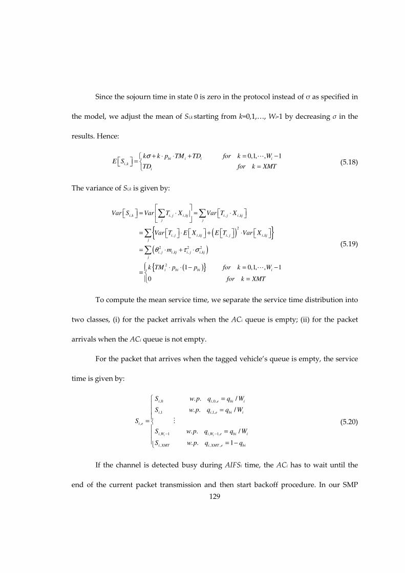
129

Since the sojourn time in state 0 is zero in the protocol instead of σ as specified in

the model, we adjust the mean of Si,k starting from k=0,1,…, Wi-1 by decreasing σ in the

results. Hence:

,

0,1, , 1bi i i i

i k

i

k k p TM TD for k WE S

TD for k XMT

σ + ⋅ ⋅ + = − = =

L

(5.18)

The variance of Si,k is given by:

( ){ }( )

( ){ }

, , , , ,

2

, , , ,

2 2 2

, , , ,

2 1 0,1, , 1

0

i k i j i kj i j i kj

j j

i j i kj i j i kj

j

i j i kj i j i kj

j

i bi bi i

Var S Var T X Var T X

Var T E X E T Var X

m

k TM p p for k W

for k XMT

θ τ σ

= ⋅ = ⋅

= ⋅ + ⋅

= ⋅ + ⋅

⋅ ⋅ − = −=

=

∑ ∑

∑

∑

L

(5.19)

To compute the mean service time, we separate the service time distribution into

two classes, (i) for the packet arrivals when the ACi queue is empty; (ii) for the packet

arrivals when the ACi queue is not empty.

For the packet that arrives when the tagged vehicle’s queue is empty, the service

time is given by:

,0 ,0,

,1 ,1,

,

, 1 , 1,

, , ,

. . /

. . /

. . /

. . 1

i i

i i e bi i

i i e bi i

i e

i W i W e bi i

i XMT i XMT e bi

S w p q q W

S w p q q W

S

S w p q q W

S w p q q

− −

=

=

= = = −

M

(5.20)

If the channel is detected busy during AIFSi time, the ACi has to wait until the

end of the current packet transmission and then start backoff procedure. In our SMP

130

model, we have neglected such waiting time. Since such waiting time is relatively small

comparing to the mean packet arrival time, it has little influence on the steady-state

probability that a vehicle is in state XMT. Hence, PDR and PRR are not influenced by

such waiting time, while it has influence on the mean transmission delay. Therefore, it is

not necessary to represent this part as an additional state into the model. We only adjust

the mean service time here to include this waiting time. When a packet transmission is

detected by the tagged vehicle’s AIFSi channel sensing time, the mean waiting time

before the ACi starts backoff procedure is half of the packet transmission. Therefore,

,0 ,0,

,1 ,1,

,

, 1 , 1,

, , ,

. . /2

. . /2

. . /2

. . 1

i i

i i

i i e bi i

i i

i i e bi i

i e

i i

i W i W e bi i

i XMT i XMT e bi

TM AIFSS w p q q W

TM AIFSS w p q q W

S

TM AIFSS w p q q W

S w p q q

− −

−+ =

− + =

= − + = = −

M

(5.21)

The mean and variance of the service time for the packet arrivals when the ACi

queue is empty are:

( )

( ) ( ) ( )

, , , , ,2

1

2 2

bi i i

i e i e i k i k e

k

i bi i bi bi i i

i

q TM AIFSE S E S q

W p TM q q TM AIFSTD

β

σ

⋅ − = = ⋅ +

− + ⋅ ⋅ ⋅ −= + +

∑

(5.22)

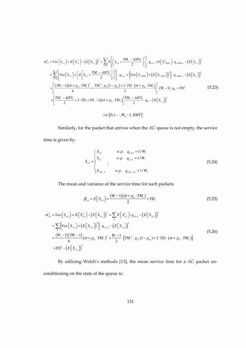
131

( ) ( )21

2 22 2 2

, , , , , , , , , , ,

0

21

, , , , ,

0

2

2

i

i

W

i ii e i e i e i e i k i k e i XMT i XMT e i e

k

W

i ii k i k i k e i XMT

k

TM AIFSVar S E S E S E S q E S q E S

TM AIFSVar S E S q Var S

σ−

=

−

=

− = = − = + ⋅ + ⋅ −

− = + + ⋅ +

∑

∑ ( ){ } ( )

( )( ) ( ) ( )( )

( )( ) ( )

2 2

, , , ,

2 2

2

2

,

2 1 1 21

6 2

2 12 2

i XMT i XMT e i e

i bi i i bi bi i bi i

i bi i

i i i ii i bi i bi i e

E S q E S

W p TM TM p p TD p TMW q TD

TM AIFS TM AIFSTD W p TM q E S

σ σ

σ

+ ⋅ −

− + ⋅ ⋅ − + ⋅ ⋅ + ⋅= + ⋅ − ⋅ +

− − + + ⋅ + − + ⋅ ⋅ −

{ }00,1, , 1,i W XMT∈ −L

(5.23)

Similarly, for the packet that arrives when the ACi queue is not empty, the service

time is given by:

,0 ,0,

,1 ,1,

,

, 1 , 1,

. . 1/

. . 1/

. . 1/i i

i i b i

i i b i

i b

i W i W b i

S w p q W

S w p q WS

S w p q W− −

=

== =

M

(5.24)

The mean and variance of the service time for such packets:

( )( ), ,

1

2

i bi i

i b i b i

W p TME S TD

σβ

− + ⋅ = = +

(5.25)

( ) ( )

( ){ } ( )

( )( )( ) ( ) ( ){ }

( )

2 22 2 2

, , , , , , , ,

2 2

, , , , ,

2 2

22

,

1 2 1 11 2

6 2

i b i b i b i b i k i k b i b

k

i k i k i k b i b

k

i i i

bi i i bi bi i bi i

i i b


Var S E S q E S

W W Wp TM TM p p TD p TM

TD E S

σ

σ σ

= = − = ⋅ −

= + ⋅ −

− − −= + ⋅ + ⋅ ⋅ − + ⋅ ⋅ + ⋅

+ −

∑

∑

(5.26)

By utilizing Welch’s methods [13], the mean service time for a ACi packet un-

conditioning on the state of the queue is:

132

[ ]( )

,

, ,1

i e

i

i i b i e

E Sβ

λ β β=

− −

(5.27)


For the results obtained from SMP models above, we know that there are nine

unknown parameters: ρ1, ρ2, ρ3, pb1, pb2, pb3, qb1, qb2, and qb3. The mean service time for ACi

shown above depends on all these nine parameters. Therefore, channel utilization ρi of

the M/G/1 queue in each vehicle depends on all nine unknown parameters. In this

section, we determine how pbi and qbi depend on these nine parameters. Next, we can use

the fixed point iteration to obtain the converged solution.

Let Ncs denote the average number of vehicles in carrier sensing range of the



2cs trN N Rβ= = (5.28)


4 2ph cs

N R N Rβ β= − = (5.29)

From the tagged vehicle’s point of view, pbi is the probability that it senses

channel busy during one time slot in the backoff process for ACi service. The channel is

detected busy can be due to two cases:

a. If this tagged vehicle is transmitting other types of message during this backoff slot, or

b. At least one neighbor (i.e., a vehicle in the transmission range of the tagged vehicle) is

transmitting any types of messages during this backoff slot. Therefore, we have:

133

( ) ( )( )( )( ) ( )

( ) ( ) ( )( )( ),1, ,2 , ,3,

31

, , ,1, ,2, ,3,

01,

31 1 1 1 1

, ,

1,

11 1 1 1 1

!

1 1

cs

cs i XMT i XMT i XMT

kk Ncs

bi i j XMT i XMT i XMT i XMT

kj j i

N P P P

i j XMT

j j i

Np P P P P e

k

P e

∞− −

== ≠

− − ⋅ − − − −

= ≠

− = − − ⋅ − − −

= − − ⋅

∑∏

∏ (5.30)

where Pi,j,XMT is the probability that ACj message (either from a neighbor or the tagged

vehicle itself) is transmitting in a backoff time slot of the tagged vehicle, which is

attempting to transmit ACi message.


capture the transmission of the ACj message is TDj-AIFSj+2σ. One extra time slot σ is the

one just before transmission and another is the one just after transmission, which can

capture the starting time instant and ending time instant of the packet transmission.

Therefore, the probability that a neighbor’s transmission is detected in the first backoff

time slot of the tagged vehicle is πi,XMT(TDj-AIFSj+2σ)/ TDj.


the time duration that captures the transmission of the ACj message is 2σ, which

captures the starting time instant of the transmission. This is because when the ACj

message transmission is detected in the first backoff time slot by the tagged vehicle, the

backoff counter will suspend and wait until the end of this transmission for further

decrement. Therefore, if the first backoff time slot detects the transmission, there is no

chance for the later backoff time slots to detect the same transmission. As a result, the

non-first backoff time slot can only detect the transmission when the starting point of the

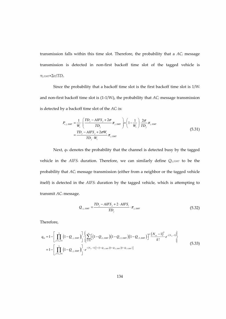
134

transmission falls within this time slot. Therefore, the probability that a ACj message

transmission is detected in non-first backoff time slot of the tagged vehicle is

πj,XMT×2σ/TDj.

Since the probability that a backoff time slot is the first backoff time slot is 1/Wi

and non-first backoff time slot is (1-1/Wi), the probability that ACj message transmission

is detected by a backoff time slot of the ACi is:

, , , ,

,

21 1 21

2

j j

i j XMT j XMT j XMT

i j i j

j j i

j XMT

j i

TD AIFSP

W TD W TD

TD AIFS W

TD W

σ σπ π

σπ

− + = ⋅ + − ⋅

− +=

⋅

(5.31)

Next, qbi denotes the probability that the channel is detected busy by the tagged

vehicle in the AIFSi duration. Therefore, we can similarly define Qi,j,XMT to be the

probability that ACj message transmission (either from a neighbor or the tagged vehicle

itself) is detected in the AIFSi duration by the tagged vehicle, which is attempting to

transmit ACi message.

, , ,

2j j i

i j XMT j XMT

j

TD AIFS AIFSQ

TDπ

− + ⋅= ⋅

(5.32)

Therefore,

( ) ( )( )( )( ) ( )

( ) ( ) ( )( )( ),1, ,2, ,3,

31

, , ,1, ,2, ,3,

01,

31 1 1 1 1

, ,

1,

11 1 1 1 1

!

1 1

cs

cs i XMT i XMT i XMT

kk Ncs

bi i j XMT i XMT i XMT i XMT

kj j i

N Q Q Q

i j XMT

j j i

Nq Q Q Q Q e

k

Q e

∞− −

== ≠

− − ⋅ − − − −

= ≠

− = − − ⋅ − − −

= − − ⋅

∑∏

∏ (5.33)

135

From the above analysis, we know that both pbi and qbi depend on all nine

parameters ρ1, ρ2, ρ3, pb1, pb2, pb3, qb1, qb2, qb3. Hence, we can use fixed-point iteration to

obtain the converged solution for all nine parameters as below:

Step 1: Initialize ρ1=ρ2=ρ3=pb1=pb2=pb3= qb1=qb2=qb3=1;

Step 2: Solve ρ1, ρ2, ρ3, pb1, pb2, pb3, qb1, qb2, qb3 according to ρi=λiE[Si] and Eqs.

(5.27)(5.30)(5.33);

Step 3: If ρ1, ρ2, ρ3, pb1, pb2, pb3, qb1, qb2, qb3 converges, then stop the iteration algorithm;

otherwise, go to step 2 with the updated ρ1, ρ2, ρ3, pb1, pb2, pb3, qb1, qb2, qb3.

By utilizing the fixed-point iteration algorithm, the parameters ρ1, ρ2, ρ3, pb1, pb2, pb3, qb1,

qb2, qb3 as well as the mean and the variance of the service time can be determined, which

are used for the MAC-layer performance indices computation in the next section.

5.4 MAC-level Performance Metrics

5.4.1 Mean transmission delay

According to the Welch’s method [13], the steady-state expected number of

packets in the tagged vehicle’s queue (including the packet in the head of the queue that

is under service) is:

[ ]( )

( )( )

2 2 2 2 2 22 2, , , ,, , ,

,, , , ,2 2 11 1

i e i e i b i bi i e i b i bi i

i

i i bi i b i e i i b i e

E Qσ β σ βλ β σ βλ λ

λ βλ β β λ β β

+ − − += + ⋅ + ⋅

−− − − −

(5.34)

Using Little’s law, the mean delay for a ACi packet transmission is:

[ ][ ]i

i

i

E QE D

λ=

(5.35)

136

5.4.2 Variance of the transmission delay

From the method proposed by Welch [13], we can get the Laplace-Stieltjes

transform for the transmission delay:

( )( )

( ) ( ) ( )

( ), , ,,

,, ,

1

1

ii e i b i ei bs D

i

i bi b i e

s s s ss E e

s s

λ ϕ ϕ ϕλβψ

λ λϕλ β β

− ⋅ − − ⋅− = = ⋅ − −− −

(5.36)

To obtain the variance of the transmission delay, we need to compute the second

moment of the transmission delay first. This can be obtained from the derivatives of the

Laplace-Stielfjes transform.

( )( )

2

2

2 0

0

''i

i i s

s

d sE D s

ds

ψψ

=

=

= =

(5.37)

Assume:

( )

( ) ( ) ( )

,

, , ,

i b

i e i b i e

a s s

b s s s s

λ λϕ

λ ϕ ϕ ϕ

= − −

= − − ⋅

Hence,

( )( )

,

, ,

1

1

i b

i

i b i e

bs

a

λβψ

λ β β

−= ⋅

− −

Therefore, we get:

( )( )

( )( )

( )

,

2

, ,

2

,

2 30, ,

0

1 ' ''

1

2 ' ' '1 '' ''''

1

i b

i

i b i e

i i i i ii b i i i i

i si ii b i e

s

b a a bs

a

a b a a bb a a bs

a a

λβψ

λ β β

λβψ

λ β β=

=

− −= ⋅

− −

−− − = ⋅ − − −

When s approaches 0, ai, and bi approach 0. Hence, we use l'Hôpital's rule to obtain the

results:

137

( )2 2

0 0

'' '' ''' ' ''' '

'

i i i i i i i i

i s i s

b a a b b a a b

a a= =

− −=

( ) ( ) ( )

( )

22 2

3 3

00

2 ' ' ' 2 ' ''' ' 3 '' '' ' 2 ' ''' 3 '' ' ' ' '''

3 '

i i i i ii i i i i i i i i i i i i

i i ss

a b a a b a a b a b a a b a b a b a

a a=

=

− − + + − − =

where:

( ),0 0' 1 'i i i bs s

a sλ ϕ= =

= − − ⋅

( ),0 0'' ''i i i bs s

a sλ ϕ= =

= − ⋅

( ),0 0''' '''i i i bs s

a sλ ϕ= =

= − ⋅

( ) ( ), ,0 0 0' ' 'i i i e i bs s s

b s sλ ϕ ϕ= = =

= ⋅ −

( ) ( ) ( ), , ,0 0 0 0

'' '' '' 2 'i i i e i b i es s s sb s s sλ ϕ ϕ ϕ

= = = = = ⋅ − −

( ) ( ) ( ), , ,0 0 0 0''' ''' ''' 3 'i i i e i b i es s s s

b s s sλ ϕ ϕ ϕ= = = =

= ⋅ − −

( ), , ,0'i e i e i es

s E Sϕ β=

= − = − ( ), , ,0'i b i b i bs

s E Sϕ β=

= − = −

( ) 2 2 2

, , , ,0''i e i e i e i es

s E Sϕ σ β=

= = + ( ) 2 2 2

, , , ,0''i b i b i b i bs

s E Sϕ σ β=

= = +

( ) 3

, , ,0'''i e i e i es

s E Sϕ γ=

= − = − ( ) 3

, , ,0'''i b i b i bs

s E Sϕ γ=

= − = −

In the above equations,

( )

( )

313 3

, , , , , , , ,

0

3 1

3 2

, , , , , ,

0

2 1

, ,

0

2

3

2 2

3

4

i

i

i

W

i i

i e i e i k i k e i XMT i XMT e

k

Wi ii i

i k i k e bi i k i k e

k k

Wi i

i k i k

k

TM AIFSE S E S q E S q

TM AIFSTM AIFSE S q q E S q

TM AIFSE S q

γ−

=

−

=

−

=

− = = + ⋅ + ⋅

−− = ⋅ + ⋅ + ⋅ ⋅

− + ⋅ ⋅

∑

∑ ∑

∑

( ) ( ){ }( )

,

3 12

3

, , , , , , ,

0

2 1

, , ,

0

3

2 2

3

4

i

i

e

Wi ii i

i k i k e bi i k i k i k e

k k

Wi i

i k i k e

k

TM AIFSTM AIFSE S q q Var S E S q

TM AIFSE S q

−

=

−

=

−− = ⋅ + ⋅ + ⋅ + ⋅

− + ⋅ ⋅

∑ ∑

∑

138

3 3

, , , , ,i b i b i k i k b

k

E S E S qγ = = ⋅ ∑

Furthermore,

( ) ( ){ }

( )

3

3

, , ,

3 2

, , , , , ,

,

, , , , , ,

, ,

3 2 2

, , , , ,

3

6

3

i k i j i kj

j

i j i kj i j i kj i l i kl

j j ll j

i j i kj i l i kl i n i kn

j l nj l n

i j i kj i j i kj i j i

j

E S E T X

E T X E T X E T X

E T X E T X E T X

m mτ θ τ σ

≠

≠ ≠

= ⋅

= ⋅ + ⋅ ⋅ ⋅ ⋅

+ ⋅ ⋅ ⋅ ⋅

= ⋅ + ⋅ ⋅ + ⋅

∑

∑ ∑

∑

∑ ( ){ }2 2

, , , ,

,

, , , , , ,

, ,

6

kj i kj i l i kl

j ll j

i j i kj i l i kl i n i kn

j l nj l n

m m

m m m

τ

τ τ τ

≠

≠ ≠

+ ⋅ ⋅

+ ⋅ ⋅ ⋅ ⋅ ⋅ ⋅

∑

∑

Therefore, based on Eqs. (5.35)(5.37), we can obtain the variance of the transmission

delay:

[ ] [ ]( )22

i i iVar D E D E D = −

(5.38)

5.4.3 Packet Delivery Ratio (PDR)

The PDR is defined as [5][7]: given a broadcast packet sent by the tagged vehicle,

the probability that all vehicles in its transmission range receive the packet successfully.

Taking account of hidden terminals, we have PDR for ACi message transmission:

( ) ( ), ,i i cs i phPDR P N P N= (5.39)

where P(Ni,cs) is the probability that no vehicles in the transmission range of the tagged

vehicle transmits any types of messages when the tagged vehicle starts ACi message

transmission, and P(Ni,ph) is the probability that no transmissions from the vehicles in the

139

potential hidden terminal area collide with the broadcast ACi packet from the tagged

vehicle.

P(Ni,cs) can also be interpreted as the no-concurrent transmission probability, i.e.,

two packets do not start transmission at the same time. Since EDCA employs a discrete-

time backoff scheme, if the backoff process is involved, a vehicle is only allowed to

transmit at the beginning of each slot time after an idle AIFSi time duration. Therefore, if

the tagged vehicle has not gone through the backoff process before transmitting the ACi

packet (with probability (1-ρi)(1-qbi)), the concurrent transmission will not occur.

Otherwise, the packet transmission is synchronized to the beginning of a slot time, and

concurrent transmission may occur if other vehicles’ transmission is also synchronized

by the backoff process. From the model, we know that the probability that a neighbor or

the tagged vehicle itself starts to transmit a ACj packet at the beginning of the same time

slot with the tagged vehicle is πj,0= πj,XMT×σ/TDj. This is because the sojourn time in state

0 is one time slot σ as shown in the SMP model, hence, πj,0 is the probability that a

vehicle starts to transmit ACj packet in the beginning of a time slot immediately after the

backoff process. Hence, P(Ni,cs) is:

( ) ( )( ) ( ) ( ) ( ) ( )( ) ( )

( ) ( )

( )( ) ( ) ( ) ( )( )( ) ( ) ( )1,0 2,0 3,0

31

, ,0 1,0 2,0 3,0

01,

31 1 1 1 1

,0

1,

11 1 1 1 1 1 1

!

1 1

1 1 1 1 1 1

cs

cs

kk Ncs

i cs i bi j

kj j i

i bi

N

i bi j i bi

j j i

NP N q e

k

q

q e qπ π π

ρ π π π π

ρ

ρ π ρ

∞− −

== ≠

− − ⋅ − − − −

= ≠

− = − − − ⋅ − ⋅ − − −

+ − −

= − − − ⋅ − ⋅ + − −

∑∏

∏

(5.40)

140

Since the transmission time for a packet is TDj-AIFSj=E[PAj]/Rd+TH+δ, the event

that a ACj packet transmission from hidden terminals collides with the tagged vehicle’s

ACi packet transmission only happens when hidden terminals start to transmit during

the vulnerable period TDj-AIFSj+TDi-AIFSi. Therefore,

( )( )

3

,

1

3

, ,

0 1

1 1

1!

ph

j j i i

ph j XMTjj

k k

ph Nj j i i

i ph j XMT

k j j

TD AIFS TD AIFSN

TD

NTD AIFS TD AIFSP N e

TD k

e

π

π

=

∞−

= =

− + − − − − ⋅

− + −= − ⋅

∏=

∑ ∏

(5.41)

Hence, the PDR can be computed. From the analytic results demonstrated in Section 5.5,

we can see that the hidden terminals problem has more impact than concurrent

transmissions on the PDR.

5.4.4 Packet Reception Ratio (PRR)



investigated at the moment that the packet is sent out [7]. Similar to the computation for

PDR, we consider both the concurrent transmission and hidden terminal effects while

computing PRR. Therefore, PRR for ACi packet transmission is:

, ,i i cc i htPRR PRR PRR=

(5.42)

The impact of the concurrent transmission and hidden terminals will be

evaluated in the following two sections.

a. Impact of concurrent transmission

141

Transmissions from nodes within a distance R away from the tagged node in the

meantime at which the tagged node transmits may cause collisions. When the tagged

vehicle starts to transmit ACi packet, no ACj packet can be transmitted at the same time

for the tagged vehicle. Therefore, the probability that there is no concurrent transmission

from the tagged vehicle is:

31

, ,0

1,

(1 )i cc j

j j i

PRR π= ≠

= −∏

(5.43)

ACj packet transmissions from vehicles within a distance R away from the tagged

vehicle in the meantime at which the tagged vehicle transmits ACi packet may cause

collisions. When the tagged node starts ACi packet transmission in the beginning of a

slot time, collisions will take place if any vehicle in the transmission range of the tagged

vehicle starts ACj packet transmission in the beginning of the same time slot. As shown

in Fig. 3.6 in Chapter 3, any vehicles transmitting any types of messages on the right

hand side of the tagged node on the origin (i.e., node in [0, R]) will result in failure of all

vehicles in [0, R] receiving the broadcast ACi packet. Hence, ratio of successfully

receiving vehicles in the range [0, R] can be expressed as:

1,0 2,0 3,0

2

, 1,0 2,0 3,0

0

1 (1 )(1 )(1 )

( )(1 )(1 )(1 )

!

kk R

i cc

k

R

RPRR e

k

e

β

β π π π

βπ π π

∞−

=

− − − − −

= − − −

=

∑

(5.44)

On the other hand, transmissions from any vehicle on the left hand side of the

tagged vehicle (i.e., vehicle in [-R, 0]) will only result in failure of some of the vehicles

receiving the broadcast ACi packet in [0, R]. Similar to analysis of the hidden terminal

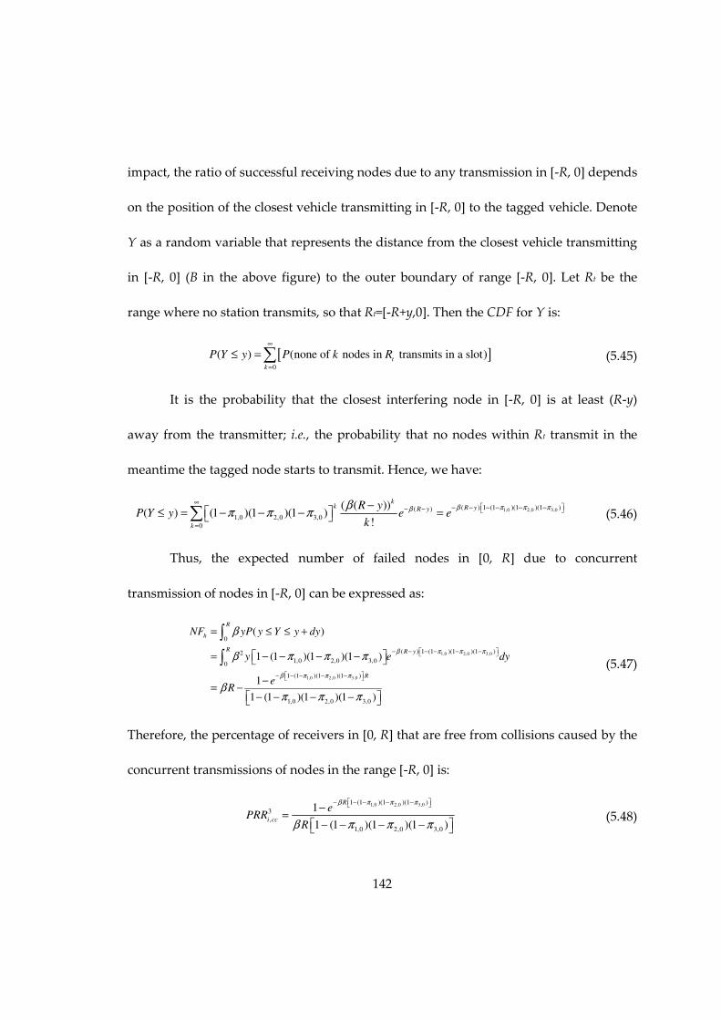
142

impact, the ratio of successful receiving nodes due to any transmission in [-R, 0] depends

on the position of the closest vehicle transmitting in [-R, 0] to the tagged vehicle. Denote

Y as a random variable that represents the distance from the closest vehicle transmitting

in [-R, 0] (B in the above figure) to the outer boundary of range [-R, 0]. Let Rt be the

range where no station transmits, so that Rt=[-R+y,0]. Then the CDF for Y is:

[ ]0

( ) (none of nodes in transmits in a slot)t

k

P Y y P k R∞

=

≤ =∑

(5.45)

It is the probability that the closest interfering node in [-R, 0] is at least (R-y)

away from the transmitter; i.e., the probability that no nodes within Rt transmit in the

meantime the tagged node starts to transmit. Hence, we have:

1,0 2,0 3,0( ) 1 (1 )(1 )(1 )( )

1,0 2,0 3,0

0

( ( ))( ) (1 )(1 )(1 )

!

kk R yR y

k

R yP Y y e e

k

β π π πββπ π π

∞ − − − − − −− −

=

− ≤ = − − − = ∑

(5.46)

Thus, the expected number of failed nodes in [0, R] due to concurrent

transmission of nodes in [-R, 0] can be expressed as:

1,0 2,0 3,0

1,0 2,0 3,0

0

( ) 1 (1 )(1 )(1 )2

1,0 2,0 3,00

1 (1 )(1 )(1 )

1,0 2,0 3,0

( )

1 (1 )(1 )(1 )

1

1 (1 )(1 )(1 )

R

h

R R y

R

NF yP y Y y dy

y e dy

eR

β π π π

β π π π

β

β π π π

βπ π π

− − − − − −

− − − − −

= ≤ ≤ +

= − − − −

−= −

− − − −

∫

∫

(5.47)

Therefore, the percentage of receivers in [0, R] that are free from collisions caused by the

concurrent transmissions of nodes in the range [-R, 0] is:

1,0 2,0 3,01 (1 )(1 )(1 )

3

,

1,0 2,0 3,0

1

1 (1 )(1 )(1 )

R

i cc

ePRR

R

β π π π

β π π π

− − − − − −=

− − − − (5.48)

143

Define PRRi,cc as the percentage of receivers in [0, R] that are free from collisions

caused by the concurrent transmissions of vehicles in the range [-R, R]. If the tagged

vehicle transmits the ACi packet without going through the backoff process, with

probability (1-ρi)(1-qbi), concurrent transmission will not occur. Otherwise, concurrent

transmissions may occur. Therefore,

( )( ) ( )( )

( )( ){ }1,0 2,0 3,0 1,0 2,0 3,0

1 2 3

, , , ,

1 (1 )(1 )(1 ) 1 (1 )(1 )(1 )3

,0

1, 1,0 2,0 3,0

1 1 1 1 1

11 1 1 (1 )

1 (1 )(1 )(1 )

i cc i bi i cc i cc i cc i bi

R R

i bi j

j j i

PRR q PRR PRR PRR q

e eq

R

β π π π β π π π

ρ ρ

ρ πβ π π π

− − − − − − − − − −

= ≠

= − − − ⋅ ⋅ ⋅ + − −

− = − − − ⋅ − ⋅ − − − −

∏

( )( )1 1i bi

qρ

+ − −

(5.49)

b. Impact of hidden terminals

We observe that the ratio of receivers affected by the hidden terminals only

depends on the position of the hidden node (referred as hidden crucial node) that has

the closest distance to boundary of the transmitter’s sensing range among all the

transmitting nodes in the potential hidden terminal area. Denote X as a random variable

that represents the distance from the hidden crucial node (A in Fig. 3.6 in Chapter 3) to

the outer boundary of [0, 2R]. Let Rs be the range in the potential hidden terminal area,

where no node transmits, such that Rs=[lcs, 2R-x],where lcs=Ncs/(2β) is carrier sensing

range of a node in the network. Then the cumulative distribution function (CDF) for X

is:

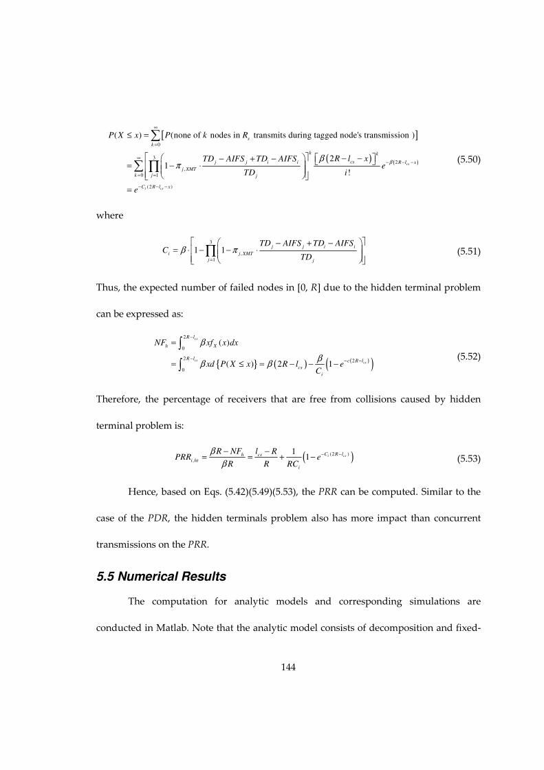
144

[ ]

( ) ( )

0

32

,

0 1

(2 )

( ) (none of nodes in transmits during tagged node's transmission )

21

!

cs

i cs

s

k

k k

csj j i i R l x

j XMT

k j j

C R l x

P X x P k R

R l xTD AIFS TD AIFSe

TD i

e

ββ

π

∞

=

∞− − −

= =

− − −

≤ =

− − − + − = − ⋅

=

∑

∑ ∏ (5.50)

where

3

,

1

1 1j j i i

i j XMT

j j

TD AIFS TD AIFSC

TDβ π

=

− + −= ⋅ − − ⋅

∏ (5.51)

Thus, the expected number of failed nodes in [0, R] due to the hidden terminal problem

can be expressed as:

{ } ( ) ( )( )

2

0

2 2

0

( )

( ) 2 1

cs

cscs

R l

h X

R l c R l

cs

i

NF xf x dx

xd P X x R l eC

β

ββ β

−

− − −

=

= ≤ = − − −

∫

∫ (5.52)

Therefore, the percentage of receivers that are free from collisions caused by hidden

terminal problem is:

( )(2 )

,

11 i csC R lh cs

i ht

i

R NF l RPRR e

R R RC

β

β− −− −

= = + − (5.53)

Hence, based on Eqs. (5.42)(5.49)(5.53), the PRR can be computed. Similar to the

case of the PDR, the hidden terminals problem also has more impact than concurrent

transmissions on the PRR.


The computation for analytic models and corresponding simulations are

conducted in Matlab. Note that the analytic model consists of decomposition and fixed-

145

point iteration while the simulative solution does not. All other assumptions are the

same in the simulation and analytic models. The results show the high accuracy of our

decomposition-based analytic approximation. We consider a freeway system where the

number of vehicles is Poisson distributed. Each vehicle on the road is equipped with

DSRC wireless capability. The control channel of DSRC is exclusively used for safety

related broadcast communication. Table 5.1 shows the parameters used in this chapter,

which reflect typical DSRC network settings in [1]. Input parameters such as packet

arrival rate, packet length, backoff window size, channel sensing time AIFS and carrier

sensing range are variables since they may have different values according to different

types of applications in practice. Therefore, we will evaluate the influence of these

varied parameters on the output measures in this section. Based on the results, we may

gain valuable insights about the parameters settings to satisfy service requirements with

respect to latency and reliability.

Table 5.1: DSRC parameters for EDCA mechanism

Parameters Values Parameters Values Tx range R 500 m Data rate Rd 24 Mbps

PHY preamble 40 µs Vehicle density β variable PLCP header 4 µs Packet arrival rate λi variable

MAC header 272 bits Packet Length PAi variable

Slot time σ 16 µs CWMin Wi-1 variable SIFS 32 µs AIFSi variable

Propagation delay δ 0 µs Carrier sensing range lcs variable

5.5.1 Influence of Packet Arrival Rate

For different applications in practice, the workloads may differ. Hence, we are

interested in the following question: Will the application with smaller arrival rate has

146

higher reliability (PDR and PRR) than the application with larger arrival rate? Intuitively

speaking, the message that rarely generated has less inference than message that

frequently generated. However, this statement is proved to be wrong by our results

presented next.

To evaluate the influence of the packet arrival rate, we set the input parameters

values as in Table 5.2. The EDCA parameters including backoff window size and AIFS

channel sensing time for different ACs are set to be different to provide service

differentiations.

Table 5.2: Parameters for packet arrival rate influence evaluation

Parameters Values for AC1, AC2, AC3

Packet arrival rate λi (#/sec) 10, 5, 2

Packet Length PAi (bytes) 200, 200, 200

CWMin Wi-1 7, 3, 3

AIFSNi 6, 3, 2

Carrier sensing range lcs R=500m

The output measures including mean transmission delay, PDR and PRR are

shown in Fig. 5.3.

0 0.02 0.04 0.06 0.08 0.1 0.12 0.14 0.16 0.18 0.20

0.5

1

1.5

2

2.5

3

3.5

4

4.5

5x 10

-4


Mea

n D

ela

y (

seco

nd

s)

AC3 analytic

AC2 analytic

AC1 analytic

AC1 simulation

AC2 simulation

AC3 simulation

0 0.02 0.04 0.06 0.08 0.1 0.12 0.14 0.16 0.18 0.20

0.1

0.2

0.3

0.4

0.5

0.6

0.7

0.8

0.9

1


Packet

Deliv

ery

Ratio

AC3 analytic

AC2 analytic

AC1 analytic

AC1 simulation

AC2 simulation

AC3 simulation

0 0.02 0.04 0.06 0.08 0.1 0.12 0.14 0.16 0.18 0.20

0.1

0.2

0.3

0.4

0.5

0.6

0.7

0.8

0.9

1


Packet

Reception R

atio

AC3 analytic

AC2 analytic

AC1 analytic

AC1 simulation

AC2 simulation

AC3 simulation

Figure 5.3: Influence of packet arrival rate

147

From the results above, we can see that mean delay, PDR and PRR from analytic

model and simulation match very well, which validate the correctness of our proposed

models. The delay is relatively small. In addition, when vehicle density increases, mean

transmission delay increases, while PDR and PRR decrease. We can also observe that,

given same network parameters, PDRs are less than PRRs. This is because that PDRs

count the number of packets that are successfully received by all intended receivers,

while PRRs count the percentage (or probability) of the intended receivers that

successfully receive a packet from a sender. PDR and PRR are almost the same for three

ACs, which means the arrival rate differentiation has little impact on PDR and PRR. In

other words, the application that rarely generates messages has almost the same

reliability with the application that frequently generates messages. The delay

differentiations are mainly due to the EDCA parameters (backoff window size and

AIFS). Hence, arrival rate has little impact to provide differentiations of transmission

delay, PDR and PRR for different priority services. Our analytic results also show that

PDR and PRR are influenced by the total arrival rate of three types of services but not

the individual arrival rate.

5.5.2 Influence of Packet Length

Besides the arrival rates, we are also interested in how to choose the packet

length for safety messages, which is addressed in this section.

148

Table 5.3: Parameters for packet length influence evaluation




CWMin Wi-1 7, 3, 3

AIFSNi 6, 3, 2


0 0.02 0.04 0.06 0.08 0.1 0.12 0.14 0.16 0.18 0.21

2

3

4

5

6x 10

-4


Mean D

ela

y (

seconds)

AC3 analytic

AC2 analytic

AC1 analytic

AC1 simulation

AC2 simulation

AC3 simulation

0 0.02 0.04 0.06 0.08 0.1 0.12 0.14 0.16 0.18 0.20

0.1

0.2

0.3

0.4

0.5

0.6

0.7

0.8

0.9

1


Packet

Deliv

ery

Ratio

AC3 analytic

AC2 analytic

AC1 analytic

AC1 simulation

AC2 simulation

AC3 simulation

0 0.02 0.04 0.06 0.08 0.1 0.12 0.14 0.16 0.18 0.20

0.1

0.2

0.3

0.4

0.5

0.6

0.7

0.8

0.9

1


Packet

Reception R

atio

AC3 analytic

AC2 analytic

AC1 analytic

AC1 simulation

AC2 simulation

AC3 simulation

Figure 5.4: Influence of packet length

The input parameters are used as in Table 5.3. The results are shown as in Fig.

5.4. From the results above, we can see that mean delay, PDR and PRR from analytic

model and simulation match very well. When vehicle density increases, mean

transmission delay will increase, while PDR and PRR will decrease. AC with larger

packet length will have higher mean transmission delay, lower PDR and lower PRR.

Therefore, we have to choose short packet length to assure high reliability and small

latency.

5.5.3 Influence of Backoff Window Size

EDCA mechanism has two important parameters to provide service

differentiation: backoff window size and channel sensing time AIFS. Higher priority

149

services are allocated with smaller backoff window size and AIFS. Hence, whether

higher priority service with smaller backoff window size has smaller latency and higher

reliability is one of the major concerns. In order to evaluate the influence of the backoff

window size on the output measures, we choose the following two sets of input

parameters:

Table 5.4: D1 for backoff window size




CWMin Wi-1 7, 3, 3

AIFSNi 6, 3, 2


Table 5.5: D2 for backoff window size




CWMin Wi-1 15, 7, 7

AIFSNi 6, 3, 2


0 0.02 0.04 0.06 0.08 0.1 0.12 0.14 0.16 0.18 0.21

2

3

4x 10

-4


Mean D

ela

y (

second)

D1:AC3 W=4

D1:AC2 W=4

D1:AC1 W=8

D2:AC3 W=8

D2:AC2 W=8

D2:AC1 W=16

0 0.02 0.04 0.06 0.08 0.1 0.12 0.14 0.16 0.18 0.20

0.1

0.2

0.3

0.4

0.5

0.6

0.7

0.8

0.9

1


Packet

Deliv

ery

Ratio

D1:AC3 W=4

D1:AC2 W=4

D1:AC1 W=8

D2:AC3 W=8

D2:AC2 W=8

D2:AC1 W=16

0 0.02 0.04 0.06 0.08 0.1 0.12 0.14 0.16 0.18 0.20

0.1

0.2

0.3

0.4

0.5

0.6

0.7

0.8

0.9

1


Packet

Reception R

atio

D1:AC3 W=4

D1:AC2 W=4

D1:AC1 W=8

D2:AC3 W=8

D2:AC2 W=8

D2:AC1 W=16

Figure 5.5: Influence of backoff window size

150

From the analytic results shown above, we can see that backoff window size only

influences transmission delay, whereas has little influence on PDR and PRR. Therefore,

smaller backoff window size only leads to smaller latency when vehicle density is

relatively high but has little impact when vehicle density is small. In addition, smaller

backoff window size does not assure the higher priority services to have higher

reliability.

5.5.4 Influence of Channel Sensing Time

Table 5.6: D1 for channel sensing time




CWMin Wi-1 7, 3, 3

AIFSNi 6, 3, 2


Table 5.7: D2 for channel sensing time




CWMin Wi-1 7, 3, 3

AIFSNi 10, 8, 6


151

0 0.02 0.04 0.06 0.08 0.1 0.12 0.14 0.16 0.18 0.21

2

3

4

5x 10

-4


Mean D

ela

y (

second)

D1:AC3 AIFS=2

D1:AC2 AIFS=3

D1:AC1 AIFS=6

D2:AC3 AIFS=6

D2:AC2 AIFS=8

D2:AC1 AIFS=10

0 0.02 0.04 0.06 0.08 0.1 0.12 0.14 0.16 0.18 0.20

0.1

0.2

0.3

0.4

0.5

0.6

0.7

0.8

0.9

1

Density (No. of Vehicles/meter)P

ac

ket

Deliv

ery

Ratio

D1:AC3 AIFS=2

D1:AC2 AIFS=3

D1:AC1 AIFS=6

D2:AC3 AIFS=6

D2:AC2 AIFS=8

D2:AC1 AIFS=10

0 0.02 0.04 0.06 0.08 0.1 0.12 0.14 0.16 0.18 0.20

0.1

0.2

0.3

0.4

0.5

0.6

0.7

0.8

0.9

1


Packe

t R

eception

Ratio

D1:AC3 AIFS=2

D1:AC2 AIFS=3

D1:AC1 AIFS=6

D2:AC3 AIFS=6

D2:AC2 AIFS=8

D2:AC1 AIFS=10

Figure 5.6: Influence of channel sensing time AIFS

As we mentioned above, besides backoff window size, another EDCA parameter

is channel sensing time AIFS. Higher priority service is usually allocated shorter AIFS to

ensure that it transmits before the lower priority services. Hence, whether higher

priority service with shorter AIFS has smaller latency and higher reliability will be

evaluated in this section. In order to evaluate the influence of the channel sensing time

on the output measures, we choose the two sets of input parameters as shown in Table

5.6 and 5.7.

From the analytic results shown above, we can see that AIFS channel sensing

time only influences transmission delay, whereas has little influence on PDR and PRR.

Shorter AIFS ensures smaller latency but does not assure higher reliability for higher

priority services.

5.5.5 Influence of Carrier Sensing Range

In practice, the carrier sensing range may differ for different types of devices.

Since large carrier sensing range can reduce hidden terminal problem, we are interested

in the significance of the carrier sensing range on the VANET safety communication

152

system’s reliability. In order to evaluate the influence of carrier sensing range, we use

two sets of input parameters:

Table 5.8: D1 for carrier sensing range




CWMin Wi-1 7, 3, 3

AIFSNi 6, 3, 2


Table 5.9: D2 for carrier sensing range




CWMin Wi-1 7, 3, 3

AIFSNi 10, 8, 6

Carrier sensing range lcs 1.5R=750m

0 0.02 0.04 0.06 0.08 0.1 0.12 0.14 0.16 0.18 0.2

2

3

4x 10

-4


Mean D

ela

y (

second)

D1:AC3 lcs=R

D1:AC2 lcs=R

D1:AC1 lcs=R

D2:AC3 lcs=1.5R

D2:AC2 lcs=1.5R

D2:AC1 lcs=1.5R

0 0.02 0.04 0.06 0.08 0.1 0.12 0.14 0.16 0.18 0.20

0.1

0.2

0.3

0.4

0.5

0.6

0.7

0.8

0.9

1


Packe

t D

eliv

ery

Ratio

D1:AC3 lcs=R

D1:AC2 lcs=R

D1:AC1 lcs=R

D2:AC3 lcs=1.5R

D2:AC2 lcs=1.5R

D2:AC1 lcs=1.5R

0 0.02 0.04 0.06 0.08 0.1 0.12 0.14 0.16 0.18 0.20

0.1

0.2

0.3

0.4

0.5

0.6

0.7

0.8

0.9

1


Pac

ket

Rece

pti

on R

ati

o

D1:AC3 lcs=R

D1:AC2 lcs=R

D1:AC1 lcs=R

D2:AC3 lcs=1.5R

D2:AC2 lcs=1.5R

D2:AC1 lcs=1.5R

Figure 5.7: Influence of carrier sensing range

We observe that increasing carrier sensing range does not have significant

influence on transmission delay, but can greatly improving PDR and PRR. This is

because of the fact that larger carrier sensing range reduces the hidden terminal

153

problem, which dominates the transmission reliability as shown in Section 5.5.6.

Therefore, we should use large carrier sensing range in practice to enhance the system

reliability.

5.5.6 Hidden terminal Vs. Concurrent Transmission

From the analysis in Section 5.5.3-5.5.5, we conclude that EDCA parameters

(backoff window size and channel sensing time AIFS) have little impact on reliability

(PDR and PRR), whereas carrier sensing range has significant impact. Since EDCA

parameters influence concurrent transmission and carrier sensing range is closely

correlated with hidden terminal problem, we may make a hypothesis that concurrent

transmission has less impact than hidden terminal problem with respect to reliability.

This hypothesis will be verified by the analytic-numeric results for AC1 service from the

analytic model using parameters in Table 5.10. As shown in Fig. 5.8, the PDR and PRR

are dominated by the hidden terminal problem’s influence. The concurrent transmission

has much less impact comparing to hidden terminal problem. This may be due to short

packet length and relatively small arrival rate for safety messages.

Table 5.10: Parameters for reliability factors evaluation




CWMin Wi-1 7, 3, 3

AIFSNi 6, 3, 2

Carrier sensing range lcs 1.2R=600m

154

0 0.02 0.04 0.06 0.08 0.1 0.12 0.14 0.16 0.18 0.20.5

0.55

0.6

0.65

0.7

0.75

0.8

0.85

0.9

0.95

1


Pro

bab

ility

PDR for AC1 service

PDR

PDR due to hidden terminal

PDR due to concurrent transmission

0 0.02 0.04 0.06 0.08 0.1 0.12 0.14 0.16 0.18 0.20.5

0.55

0.6

0.65

0.7

0.75

0.8

0.85

0.9

0.95

1


Pro

babili

ty

PRR for AC1 service

PRR

PRR due to hidden terminal

PRR due to concurrent transmission

Figure 5.8: Hidden terminal Vs. concurrent transmission

5.5.7 One Vs. Multiple Types of Services

Since EDCA mechanism is supposed to provide service differentiations for

different priority services, we want to compare the output measures for one type of

service and multiple types of services using EDCA. Therefore, the following two set of

parameters are used:

Table 5.11: Parameters for one type of service

Parameters Values

Packet arrival rate λ (#/sec) 10

Packet Length PA (bytes) 200

CWMin W-1 3

AIFSN 3


Table 5.12: Parameters for multiple types of services using EDCA




CWMin Wi-1 7, 3, 3

AIFSNi 6, 3, 2


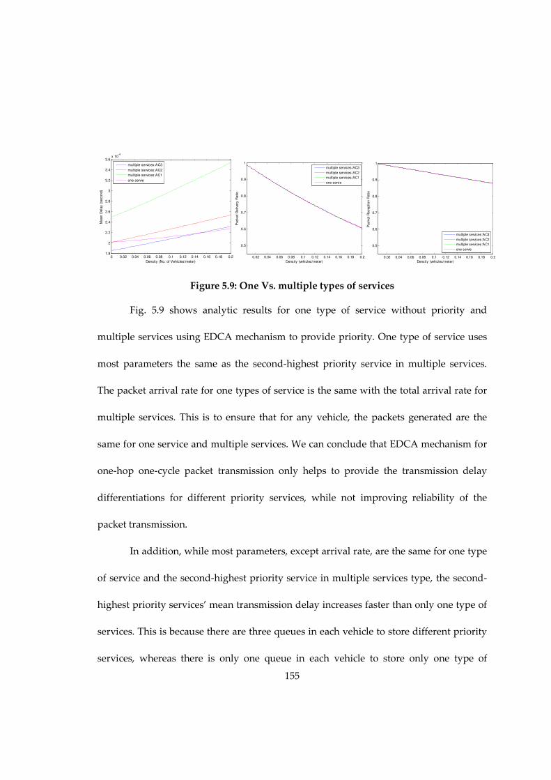
155

0 0.02 0.04 0.06 0.08 0.1 0.12 0.14 0.16 0.18 0.21.8

2

2.2

2.4

2.6

2.8

3

3.2

3.4

3.6x 10

-4


Mean

Dela

y (

se

con

d)

multiple services:AC3



one servie

0.02 0.04 0.06 0.08 0.1 0.12 0.14 0.16 0.18 0.2

0.5

0.6

0.7

0.8

0.9

1


Packet

Delivery

Ratio




one servie

0.02 0.04 0.06 0.08 0.1 0.12 0.14 0.16 0.18 0.2

0.5

0.6

0.7

0.8

0.9

1


Packet

Reception R

atio




one servie

Figure 5.9: One Vs. multiple types of services

Fig. 5.9 shows analytic results for one type of service without priority and

multiple services using EDCA mechanism to provide priority. One type of service uses

most parameters the same as the second-highest priority service in multiple services.

The packet arrival rate for one types of service is the same with the total arrival rate for

multiple services. This is to ensure that for any vehicle, the packets generated are the

same for one service and multiple services. We can conclude that EDCA mechanism for

one-hop one-cycle packet transmission only helps to provide the transmission delay

differentiations for different priority services, while not improving reliability of the

packet transmission.

In addition, while most parameters, except arrival rate, are the same for one type

of service and the second-highest priority service in multiple services type, the second-

highest priority services’ mean transmission delay increases faster than only one type of

services. This is because there are three queues in each vehicle to store different priority

services, whereas there is only one queue in each vehicle to store only one type of

156

service. Therefore, the competition is more severe for multiple services than only one

type of service.

5.5.8 Preemptive Priority

Since EDCA mechanism for one-hop one-cycle safety communication does not

help improving reliability of the packet transmission as shown in the previous section,

other enhancement strategies need to be proposed and evaluated to improve reliability.

One possible strategy is that we can set preemptive priority for the highest priority

service by using the following input parameters:

Table 5.13: Parameters for preemptive priority




CWMin Wi-1 7, 3, 0

AIFSNi 6, 3, 1


0 0.02 0.04 0.06 0.08 0.1 0.12 0.14 0.16 0.18 0.20

1

2

3

4x 10

-4


Mea

n D

ela

y (

sec

ond

s)

AC3 analytic

AC2 analytic

AC1 analytic

AC1 simulation

AC2 simulation

AC3 simulation

0 0.02 0.04 0.06 0.08 0.1 0.12 0.14 0.16 0.18 0.20

0.1

0.2

0.3

0.4

0.5

0.6

0.7

0.8

0.9

1


Packet

Deliv

ery

Ratio

AC3 analytic

AC2 analytic

AC1 analytic

AC1 simulation

AC2 simulation

AC3 simulation

0 0.02 0.04 0.06 0.08 0.1 0.12 0.14 0.16 0.18 0.20

0.1

0.2

0.3

0.4

0.5

0.6

0.7

0.8

0.9

1


Packet

Reception R

atio

AC3 analytic

AC2 analytic

AC1 analytic

AC1 simulation

AC2 simulation

AC3 simulation

Figure 5.10: Preemptive priority results

The chosen input parameters ensure that for the highest priority service, it will

transmit first when other types of services coexist at the same time because of its shortest

157

channel sensing time and no backoff process. From Fig. 5.10, we can see that preemptive

priority only provides delay differentiations whereas not help improving PDR and PRR.

Therefore, preemptive priority is not a good strategy to enhance reliability. This is

because of the fact that preemptive priority only helps to reduce concurrent

transmission and not influence hidden terminals problem, which dominates the

reliability.

5.5.9 Strict Priority

Another possible strategy to enhance performance is utilizing strict priority [92].

Strict priority can be implemented by using distinct AIFS for different priority services.

The lower priority service’s channel sensing time AIFS should be larger than the AIFS

plus the maximum backoff window size of the higher priority services.

0 0.02 0.04 0.06 0.08 0.1 0.12 0.14 0.16 0.18 0.2

1.6

1.7

1.8

1.9

2

2.1

2.2

2.3

2.4

2.5x 10

-4


Mean D

ela

y (

seconds)

AC3 analytic

AC2 analytic

AC1 analytic

AC1 simulation

AC2 simulation

AC3 simulation

0 0.02 0.04 0.06 0.08 0.1 0.12 0.14 0.16 0.18 0.20

0.1

0.2

0.3

0.4

0.5

0.6

0.7

0.8

0.9

1


Packet

Deliv

ery

Ratio

AC3 analytic

AC2 analytic

AC1 analytic

AC1 simulation

AC2 simulation

AC3 simulation

0 0.02 0.04 0.06 0.08 0.1 0.12 0.14 0.16 0.18 0.20

0.1

0.2

0.3

0.4

0.5

0.6

0.7

0.8

0.9

1


Packet

Reception R

atio

AC3 analytic

AC2 analytic

AC1 analytic

AC1 simulation

AC2 simulation

AC3 simulation

Figure 5.11: Strict priority results

From Fig. 5.11, we observe that strict priority also only provides delay

differentiations whereas not help improving PDR and PRR. Therefore, strict priority is

not a good strategy to enhance reliability. This is because of the fact that strict priority

158

only helps to reduce concurrent transmission and not influence hidden terminals

problem, which dominates the reliability.

5.5.10 Variance of Transmission Delay

According to Section 5.4.2, we can obtain the analytic-numeric results for the

variance of the transmission delay. The following input parameters are used:

Table 5.14: Parameters for variance computation




CWMin Wi-1 7, 3, 3

AIFSNi 6, 3, 2


0 0.02 0.04 0.06 0.08 0.1 0.12 0.14 0.16 0.18 0.20

0.2

0.4

0.6

0.8

1

1.2

1.4x 10

-8


Va

riance o

f th

e D

ela

y (

second2

)

AC3

AC2

AC1

Figure 5.12: Variance of the transmission delay

From Fig. 5.12, we can see that the variance for the transmission delay is very

small even when the vehicle density is high. Since we assume packet inter-arrival time is

exponential distributed and set the packet arrival rate the same for three types of

159

services, the difference of the variance are mainly due to the EDCA parameters (backoff

window size and AIFS).

5.6 GI/G/1 Queue Extension

In the previous analytic model, M/G/1 queue interacting with SMP model, we

assume the packet inter-arrival time is exponential distribution. However, in real

scenarios, the inter-arrival time can be more generally distributed. Therefore, we are

interested in the packet transmissions when packet inter-arrival time is general

independent distribution, which can be modeled as GI/G/1 queue instead. In this

section, we assume only the mean and variance of the packet inter-arrival time are

provided whereas its distribution is unknown. Therefore, the computation methods

presented in Section 5.3 and Section 5.4 cannot be directly used. The corresponding

modifications for the GI/G/1 queue interacting with SMP models are shown as follows.

5.6.1 SMP Model

The structure of the SMP model for the GI/G/1 queue case is the same as that for

the M/G/1 queue. One exception is that the sojourn time in state idle will be different.

Hence, the mean and variance of the sojourn time in each state is adjusted to:

[ ]

[ ]

0 1 2

, ,

0,1, 1

, ,

/

i

i

i H PA i W

i j i j

i H i d i

i i

j W

TM T M AIFS j D D DE T

TD T E PA R AIFS j XMT

E A AIFS j idle

σ

δτ

δ

−

= −

= + + + = = = = + + + =

+ =

L

L

(5.54)

160

[ ]

2

, , 0 1 2

0 0,1, 1

0 , , ,i

i

i j i j W

i

j W

Var T j D D D XMT

Var A j idle

θ −

= −

= = =

=

L

L

(5.55)

where E[Ai] and Var[Ai] represent the mean and variance of the packet inter-arrival time.

Therefore, the steady-state probability that a vehicle is in state XMT is adjusted to:

( ) ( ) ( ) ( ) [ ]( ),

2

1 2 2 1

i

i XMT

i bi i bi i i bi i i i i i

TD

q p TM W p TM TD E A AIFSπ

ρ ρ σ σ ρ

⋅=

+ − + ⋅ + − ⋅ + ⋅ + − + (5.56)


Since the current queueing model is GI/G/1 instead of M/G/1, Welch’s method to

compute the mean of the service time for M/G/1 queue does not apply. Therefore, we

use direct initial probability allocation method in this section to compute the mean

service time.

The mean and variance of the service time starting from state k for ACi message

(Si,k) are the same with M/G/1 queuing model as shown in Section 5.3.2:

( ),

0,1, , 1bi i i i

i k

i

k p TM TD for k WE S

TD for k XMT

σ + ⋅ + = − = =

L

(5.57)

( )2

,

1 0,1, , 1

0

i bi bi i

i k

k TM p p for k WVar S

for k XMT

⋅ ⋅ − = − = =

L

(5.58)

For a newly generated packet, if the channel is detected busy during AIFSi time,

the tagged vehicle has to wait until the end of the current packet transmission and then

start backoff procedure. In our SMP model, we have neglected such waiting time. Since

such waiting time is relatively small comparing to the mean packet arrival time, it has

161

little influence on the steady-state probability that a vehicle is in state XMT. Hence, PDR

and PRR are not influenced by such waiting time, while it has some influence on the

mean transmission delay. Therefore, it is not necessary to represent this part as an

additional state into the model. We only adjust the mean service time here to include

this waiting time. When a packet transmission is detected by the tagged vehicle’s AIFSi

channel sensing time, the mean waiting time before the tagged vehicle starts backoff

procedure is half of the packet transmission. Therefore, the service time for ACi message

will be:

( )( )

( )( )

,0 ,0 ,0

,1 ,1 ,1

, 1 , 1 , 1

, ,0 ,

, 1 ,1 , 1

,2 1 , 1

. . /

. . /

. . /

. . 1 /2

. . 1 /2

i i i

i i

i i

i i

i i i i i

i i i i i

i W i W i W i i

i i

i W i i W i bi i

i i i

i W i i W i bi i

i

i W i W

SI S w p q W

SI S w p q W

SI S w p q W

TM AIFSSI S w p q q W

S TM AIFSSI S w p q q W

TM AIFSSI S

ρ

ρ

ρ

ρ

ρ

− − −

+ +

− −

= =

= =

= =

−= + = −

= −= + = −

−= +

M

M

( )( )

( )( )

,2 1

,2 , ,2

. . 1 /2

. . 1 1

i

i i

i

i W i bi i

i W i XMT i W i bi

w p q q W

SI S w p q q

ρ

ρ

−

= −

= = − −

(5.59)

with

( )

( )( )( )

,

0,1, , 1

, 1, ,2 12

2

bi i i i

i i

i k i bi i i i i i

i i

k p TM TD for k W

TM AIFSE SI k W p TM TD for k W W W

TD for k W

σ

σ

+ ⋅ + = −

− = − + ⋅ + + = + −

=

L

L

(5.60)

162

( )

( ) ( )

2

2

,

1 0,1, , 1

1 , 1, ,2 1

0 2

i bi bi i

i k i i bi bi i i i

i

k TM p p for k W

Var SI k W TM p p for k W W W

for k W

⋅ ⋅ − = −

= − ⋅ ⋅ − = + −

=

L

L

(5.61)

Hence, the mean and variance of the service time is given by:

[ ]( ) ( )( ) ( ) ( ) ( )

, ,

1 1 1 1 1

2 2

bi i i bi i i bi i i

i i k i k i

k

p TM q W q TM AIFSE S E SI q TD

σ ρ ρ+ ⋅ − − − − − ⋅ − = ⋅ = + + ∑ (5.62)

[ ] [ ]( ) [ ]( )

( ){ } [ ]( )

( ) ( ) ( ) ( )( ) ( )( )

( )( )

22 22 2

, ,

0

22 2

, , ,

0

2 2

2

2 1 1 21 1 1 1

6 2

2 12

i

i

W

i i i i k i k i

k

W

i k i k i k i

k

bi i i i bi bi i bi i

i i bi

i ii i bi i i

Var S E S E S E SI q E S

Var SI E SI q E S

p TM W TM p p TD p TMW q

TM AIFSTD TD p TM W

σ σρ

σ

=

=

= − = ⋅ −

= + ⋅ −

+ ⋅ − − + ⋅ ⋅ + ⋅= + − − − −

−+ + + ⋅ + + ⋅ −

∑

∑

( ) [ ]( )2

12

i ii bi i

TM AIFSq E Sρ

− − −

(5.63)


The fixed point iteration procedure is exactly the same as the M/G/1 queue

interacting with SMP, except that:

[ ][ ]

i

i

i

E S

E Aρ = (5.64)



Welch’s method cannot be used for the mean delay computation. Therefore, we

use the approximation formulas proposed by Whitt to compute the mean and variance

of the queue waiting time for GI/G/1 queue instead:

163

[ ] [ ]( )

( ) [ ]

( )

2 22 2 2 2

/ /12 2 1 2 1

i ii i i iS A i iS A S A i

i i i i iM M

i i i

c c E Sc c c cE W E W

ρρψ ψ ψ

µ ρ ρ

++ +≈ = ⋅ =

− − (5.65)

where

( )

( )( )

( )

( )

2 2

2 2 2

2 2

2 2

2 1 2 2

32 2 2 2

2 2

2 2

42

4 3

32

2

i i

i i i

i i

i i

i

i ii

i i i i

i i

i i

A S

A S S

A S

A S

i

A S

S A S A

A S

A S

c cc c c

if c cc c

c cc c e c c

if c cc c

ρ

ρ

ψ− −

+− + Ψ ≥

−=

+− + + Ψ

≤ +

The function Ψ(.) is defined as:

( ) ( ) ( )2

2

2 12 2 1

3 2

1 1

0.5 0.5 0 1

ii

i

i

c

i

i

if c

ce if c

ρ

ρ

−− −

≥

Ψ = + ≤ ≤

Hence, based on Eqs. (5.62)(5.65), the mean of the transmission delay for ACi message is:

[ ] [ ] [ ]i i iE D E W E S= + (5.66)

5.6.4.2 Variance of Transmission Delay

To derive the variance of the transmission delay, we use the formulas proposed

by Whitt for the squared coefficient of variation of the steady-state waiting time in a

GI/G/m queue. For a GI/G/1 queue, the approximation reduces to:

( )

( )( )

( )

3

22

2

4 12 0

3 1

0

i

i

i

i S

i i

S

W

i

dP W

cc

P W

ρρ

−+ − >

+≈

>

where

164

[ ]( )

3

3

3i

i

S

i

E Sd

E S

=

( ) ( )( )

( )( ) ( )( )

2

3 3

, ,

0

31 2 1

3 3

, , ,

0

1

3 3

, ,

0

1 1 1

2

1 1 1 1 1

i

i i

i

i

i

W

i i k i k

k

W Wi bi i bii i i

i k i k W i XMT

k k Wi i i

Wi bi i bi

i k i XMT

k i i

E S E SI q

q qTM AIFSE S E S E S

W W W

q q TE S E S

W W

ρ ρρ

ρ ρ

=

− −

−= =

−

=

= ⋅

− − −− = ⋅ + + ⋅ + ⋅

− − − − − = ⋅ + ⋅ +

∑

∑ ∑

∑ ( )

( ) ( ) ( ) ( )

3

21 1

2

, ,

0 0

12

3 1 3 1

2 4

i i

i i

i bi

W Wi i i bi i i i bi

i k i k

k ki i

M AIFSq

TM AIFS q TM AIFS qE S E S

W W

ρ

ρ ρ− −

= =

− ⋅ −

− − − − + ⋅ ⋅ + ⋅ ⋅ ∑ ∑

In the above equation,

( )( )

( )

( )( )( ) ( ) ( ) ( )

1

,

0

22

, , ,

2 212 2

,

0

3

, , ,

1

2

1 2 11 2 1

6 2

i

i

Wi bi i

i k i i

k

i k i k i k

Wi i bi i i bi bii i bi i

i k i i

k

i k i j i kj

j

W p TME S TD W

E S Var S E S

W TD p TM TM p pW W p TME S TD W

E S E T X

σ

σσ

−

=

−

=

− + ⋅ = +

= +

− ⋅ ⋅ + ⋅ + −− − + ⋅ = + +

= ⋅

∑

∑

∑

( ) ( ){ }

( ) ( )

3

3 2

, , , , , , , , , , , ,

, , ,

3 2 2 2 2

, , , , , , , , ,

3 6

3

i j i kj i j i kj i l i kl i j i kj i l i kl i n i kn

j j l j l nl j j l n

i j i kj i j i kj i j i kj i kj i l i k

j

E T X E T X E T X E T X E T X E T X

m m m mτ θ τ σ τ

≠ ≠ ≠

= ⋅ + ⋅ ⋅ ⋅ ⋅ + ⋅ ⋅ ⋅ ⋅

= ⋅ + ⋅ ⋅ + ⋅ + ⋅ ⋅

∑ ∑ ∑

∑ { } , , , , , ,

, , ,

6l i j i kj i l i kl i n i kn

j l j l nl j j l n

m m mτ τ τ

≠ ≠ ≠

+ ⋅ ⋅ ⋅ ⋅ ⋅ ⋅∑ ∑

Whitt also gives the following approximation for P(Wi>0):

( ) ( )2 2

1 20 1i i iP W ρ π ρ π> ≈ + −

where

165

( )( )

( )

( )( )( )( )

2

2 2

1

2

2

1 11

min 1,1 1

1 2 1 1min 1,

1 1

i

i i

i

S i

A S

i

i

A i

i

i

c

c c

c

ρ

π ρρ

ρπ ρ

ρ

+ − − Φ + =

− Φ −

− Φ + − =

− Φ −

Φ(.) is the pdf for the standard normal distribution. Therefore, the variance of the

queuing waiting time is given by:

[ ] [ ]( )22

ii W iVar W c E W= ⋅ (5.67)

Assuming the queue waiting time and service time are independent and based on Eqs.

(5.63)(5.67), we can approximate the variance of the transmission delay as:

[ ] [ ] [ ]i i iVar D Var W Var S≈ + (5.68)

5.6.4.3 PDR

The PDR computation formula is the same as M/G/1 queue.

5.6.4.4 PRR

The PDR computation formula is the same as M/G/1 queue.

5.6.4.5 Numerical Results

To evaluate the correctness and accuracy of the method for GI/G/1 queue case,

the parameters in Table 5.15 are used for the numeric results computation. The numeric

results for the analytic model are shown in Fig. 5.13.

166

Table 5.15: Parameters for GI/G/1 queue


Mean packet inter-arrival time E[Ai]

(sec)

0.5, 0.5, 0.5

Variance of packet inter-arrival

time Var[Ai] (sec2)

0.25, 0.25, 0.25


CWMin Wi-1 7, 3, 3

AIFSNi 6, 3, 2


0 0.02 0.04 0.06 0.08 0.1 0.12 0.14 0.16 0.18 0.21.8

2

2.2

2.4

2.6

2.8

3

3.2x 10

-4


Mea

n D

ela

y (

sec

ond)

AC3

AC2

AC1

0 0.02 0.04 0.06 0.08 0.1 0.12 0.14 0.16 0.18 0.20

0.2

0.4

0.6

0.8

1

1.2

1.4x 10

-8


Va

rianc

e o

f th

e D

ela

y (

secon

d2)

AC3

AC2

AC1

0 0.02 0.04 0.06 0.08 0.1 0.12 0.14 0.16 0.18 0.20

0.1

0.2

0.3

0.4

0.5

0.6

0.7

0.8

0.9

1


Pa

cke

t D

eliv

ery

Ratio

AC3

AC2

AC1

0 0.02 0.04 0.06 0.08 0.1 0.12 0.14 0.16 0.18 0.20

0.1

0.2

0.3

0.4

0.5

0.6

0.7

0.8

0.9

1


Packet

Reception R

atio

AC3

AC2

AC1

Figure 5.13: Output measures for GI/G/1 queue

167

Comparing to the M/G/1 queue case, we set the input parameters for M/G/1

queue as the counterpart of GI/G/1 queue, where the mean and variance of the packet

inter-arrival time is the same as shown in Table 5.16.

Table 5.16: Parameters for GI/G/1 queue




CWMin Wi-1 7, 3, 3

AIFSNi 6, 3, 2


0 0.02 0.04 0.06 0.08 0.1 0.12 0.14 0.16 0.18 0.21.8

2

2.2

2.4

2.6

2.8

3

3.2x 10

-4


Mean D

ela

y (

second)

AC3

AC2

AC1

0 0.02 0.04 0.06 0.08 0.1 0.12 0.14 0.16 0.18 0.20

0.2

0.4

0.6

0.8

1

1.2

1.4x 10

-8


Variance o

f th

e D

ela

y (

second2

)

AC3

AC2

AC1

0 0.02 0.04 0.06 0.08 0.1 0.12 0.14 0.16 0.18 0.20

0.1

0.2

0.3

0.4

0.5

0.6

0.7

0.8

0.9

1


Packet

Deliv

ery

Ratio

AC3

AC2

AC1

0 0.02 0.04 0.06 0.08 0.1 0.12 0.14 0.16 0.18 0.2

0

0.1

0.2

0.3

0.4

0.5

0.6

0.7

0.8

0.9

1


Packet

Reception R

atio

AC3

AC2

AC1

Figure 5.14: Output measures for M/G/1 queue

168

From the results, we observe that for GI/G/1 queue with the same mean and

variance of the packet inter-arrival time as M/G/1 queue, they have almost the same

output measures. Such close match validates the correctness and accuracy of our

analytic model for the GI/G/1 queue case. In addition, from the numerical results, we

conclude that the mean and variance of the transmission delay is dominated by the

mean and variance of the service time respectively. Queueing waiting time occupies a

very small portion of the transmission delay.

5.7 A Case Study

In this section, we apply our proposed model to a case study for Vehicle Safety

Communications (VSC) vehicles to reflect MAC-layer performances in real scenarios.

Since currently there is no standard on the applications that will be deployed in future

and corresponding implementations (i.e., channel allocation and priority setting), we

propose the applications over the control channel with three priorities based on [53] as

shown in Table 5.17. Important input parameters for VSC vehicles, including packet

length and transmission range, are chosen from the testbed used in GM’s EN-V concept

vehicles. Electric Networked-Vehicles (EN-V) are capable of low-speed autonomous

driving in both indoor and outdoor controlled environments. State-of-the-art DSRC-

based V2X communication, GPS, in-vehicle vision and ultrasonic sensors were used in

combination with GM R&D-developed motion control, dead reckoning, collision

avoidance and platoon control algorithms and software to achieve the intended

169

autonomous driving capability. The other parameters for VSC vehicles are chosen in the

way to reflect typical DSRC network settings in [1] and default EDCA parameter

settings in [93] as shown in Table 5.18.

Table 5.17: Safety applications over the control channel

Access

Category

Priority

Level Applications Description Arrival Rate

AC3 Highest

Emergency

Electronic

Brake Light

A vehicle braking hard broadcasts a

warning message to approaching

vehicles in its neighborhood for the

duration of the event

5.6e-5~2.8e-4

packets/sec

(every 1~5 hours a

packet)

AC2 Second

Cooperative

Collision

Warning

(CCW)

A vehicle actively monitors kinematics

status messages from vehicles in its

neighborhood to warn of potential

collisions

2~10 packets/sec

(every 0.1~0.5 sec a

packet)

AC1 Lowest

Road Feature

Notification

(RFN)

A vehicle detecting a road feature (e.g.,

road curve, hill, road grade) notifies

approaching vehicles in its neighborhood

2.8e-4~5.6e-4

packets/sec

(every 30~60 min a

packet)

Table 5.18: Parameters setting for case study


Tx range R 300 m Data rate Rd 24 Mbps

PHY preamble 40 µs Vehicle density β Variable

PLCP header 4 µs Packet arrival rate λi Variable

MAC header 272 bits Packet Length PAi (bytes) [119, 102, 102]

Slot time σ 16 µs CWMin Wi-1 [15, 7, 3]

SIFS 32 µs AIFSi [6, 3, 2]

Propagation delay δ 0 µs Carrier sensing range lcs 1.2R=360m

Since the packet arrival rates for three types of services are variable within the

range in Table 5.17, we evaluate the upper and lower bound respectively in the next

step.

170

For the lower bound, the packet arrival rates are [λAC1, λAC2, λAC3]=[ 2.8e-4, 2, 5.6e-

5]. Fig. 5.15 shows the output measures.

0 0.05 0.1 0.15 0.21

1.4

1.8

2.2

2.6

3

3.4

3.8

4.2

4.5x 10

-4


Me

an

De

lay

(s

ec

on

d)

AC3 analytic

AC2 analytic

AC1 analytic

AC3 simulation

AC2 simulation

AC1 simulation

0 0.05 0.1 0.15 0.20.9

0.91

0.92

0.93

0.94

0.95

0.96

0.97

0.98

0.99

1


Pa

ck

et

De

live

ry R

ati

o

AC3 analytic

AC2 analytic

AC1 analytic

AC3 simulation

AC2 simulation

AC1 simulation

0 0.05 0.1 0.15 0.20.9

0.91

0.92

0.93

0.94

0.95

0.96

0.97

0.98

0.99

1


Pa

ck

et

Re

ce

pti

on

Ra

tio

AC3 analytic

AC2 analytic

AC1 analytic

AC3 simulaiton

AC2 simulation

AC1 simulation

Figure 5.15: Applications with lower bound packet arrival rates

For the upper bound, the packet arrival rates are [λAC1, λAC2, λAC3]=[ 5.6e-4, 10,

2.8e-4]. Fig. 5.16 shows the output measures.

0 0.02 0.04 0.06 0.08 0.1 0.12 0.14 0.16 0.18 0.2

1.5

2

2.5

3

3.5

4

4.5x 10

-4


Mean D

ela

y (

second)

AC3 analytic

AC2 analytic

AC1 analytic

AC3 simulation

AC2 simulation

AC1 simulation

0 0.02 0.04 0.06 0.08 0.1 0.12 0.14 0.16 0.18 0.20.8

0.82

0.84

0.86

0.88

0.9

0.92

0.94

0.96

0.98

1


Packet

Deliv

ery

Ratio

AC3 analytic

AC2 analytic

AC1 analytic

AC3 simulation

AC2 simulation

AC1 simulation

0 0.02 0.04 0.06 0.08 0.1 0.12 0.14 0.16 0.18 0.20.8

0.82

0.84

0.86

0.88

0.9

0.92

0.94

0.96

0.98

1


Packet

Reception R

atio

AC3 analytic

AC2 analytic

AC1 analytic

AC3 simulation

AC2 simulation

AC1 simulation

Figure 5.16: Applications with upper bound packet arrival rates

From the results, we can see that the analytic matches with the simulation very

well. In addition, we observe that when the total packet arrival rate becomes large, the

delay increases whereas the PDR and PRR decrease. The delay differentiations are

mainly due to EDCA parameters (backoff window size and AIFS) as shown in Section

5.5. Furthermore, even though the packet length for AC1 is different from the other two

171

types of services, the reliability does not show much difference because the difference on

packet length is relatively small.

5.8 Conclusions

In this research, a more general and accurate analytic model using SMP

interacting with an M/G/1 or GI/G/1 queue has been developed to characterize the

behavior of DSRC for highway safety communications with multiple types of services

with priority using EDCA mechanism. In a tagged vehicle, we use different queues to

store different types of messages and construct separating SMP models for each type of

safety message services. These separating SMP models interact with each other and also

with their own corresponding M/G/1 queues. Fixed-point iteration is used to obtain the

converged solution. New proposed analytic model also facilitates the accurate

evaluation of hidden terminal impact that is one of major factors for degradation of the

reliability, which has not been properly or precisely addressed in the previous work.

Both PDR and PRR, the two very important reliability metrics for DSRC safety-related

services, are analytically derived using the new model structure. The model is cross

validated against simulations. Moreover, the analysis with different input parameters is

used to suggest better parameter settings that will improve the MAC-layer performance

by decreasing the mean delay, increasing PDR and PRR. A case study is conducted

based on the testbed for GM’s EN-V concept vehicles to provide insights for real

scenarios.

172

From our analysis, several conclusions and observations are made. First, PDR

and PRR are dominated by hidden terminal problem whereas concurrent transmission

has little impact. In addition, higher priority service should choose shorter packet

length, higher data rate and larger carrier sensing range to ensure high packet

transmission reliability. Furthermore, the EDCA mechanism can only provide service

differentiation in terms of transmission delay, but is not helpful to improve the

reliability for higher priority services.

Above all, the proposed model and conclusions will be beneficial to the analysis,

design, and network parameter optimization for required MAC-layer performance and

reliability of DSRC VANET for multiple types of safety-related services. Based on the

proposed model, more practical models for more applications can be developed in

future.

173

6. Multi-channel Operation Evaluation

6.1 Motivation

Dedicated Short Range Communication (DSRC) band consists of seven channels,

one control channel (CCH) and six service channels (SCHs). IEEE 1609.4 architecture [63]

extends MAC layer operation and defines a channel switching protocol to enable a

DSRC radio to operate efficiently on multiple DSRC channels. The default access mode

in IEE 1609.4 is alternating access scheme in which the channel time is divided into

synchronization periods with a fixed length of 100 ms, consisting of CCH and SCH

intervals as shown in Fig. 1.1 in Chapter 1. All vehicles are assumed to have access to

Universal Coordinated Time (UTC) (e.g., achieved via GPS). During the CCH interval,

all vehicles tune on the CCH frequency for safety-related and system management data

exchange. During the SCH interval, vehicles switch to one of the SCH frequencies for

safety or non-safety related services been provided. 4 ms guard time is set at the

beginning of each interval to account for switching delay and time inaccuracy. Basic

Safety Message (BSM) [45][46] is one type of messages broadcasted in CCH interval to

announce the status information of a vehicle (i.e., position, speed, direction) to its

neighbors. Many safety applications rely on the timely and reliable transmissions of

such information to provide satisfactory services.

The safety message dissemination on CCH has been extensively evaluated by

either simulation or analytic model, but most of them have not considered the channel

174

switching for multi-channel operations and its impact on system performances. The

performance of multi-channel operations for safety messages have been evaluated in

[61][64][67]. Chen. [61] evaluated three access modes of the communication for a single

radio and the one with optimized scheduling has shown to effectively avoid

synchronization collisions associated with naïve use of channel switching access. Hong.

[64] proposed three alternative approaches for V2V safety communications in a multi-

channel environment for single-radio and multi-radio vehicle accommodation. Du. [67]

assessed performance of periodic beacon message transmission in CCH intervals with

respect to number of vehicles in the system. However, they are all based on simulations

in either NS2 or NCTUns and only MAC-level performance metrics (i.e., message

reception probability, transmission delay) is evaluated. Few analytic models [26][65][66]

have been proposed to characterize the MAC-level performance of safety messages

broadcasting on CCH intervals. Campolo. [26] proposed a recursive method to assess

the basic access mode for channel switching operation in which synchronization

collisions remain a severe problem. In addition, hidden terminal problem, which is one

of major factors for degradation of packet delivery reliability, is omitted in this work.

Misic. [65] investigated the performance of a single-radio supporting several traffic

combinations, each of which presents a mix of traffic classes, over control and service

channels based on Markov chain. However, no simulation is conducted to validate the

accuracy of their proposed model. Ghandour. [66] constructed analytic models for

175

upper-bound on the packet delivery delay of safety broadcast messages in multi-channel

environment and validated through simulations in NS2. These work on analytic models

only derived very few MAC-level performances (i.e., transmission delay, packet

reception probability) and channel fading effect has not been considered to characterize

practical communication environment.

In this work, we develop a detailed analytic model based on SMP [9] to

characterize both MAC and application-level performance of BSM dissemination in

CCH interval for multi-channel operations in a single-radio device incorporating

channel switching mechanism. Synchronization collisions [45] are avoided through

optimized scheduling [61]. BSM service time distribution is derived using Laplace-

Stieltjes transform based on the proposed SMP model. Next, fixed-point iteration method

is used to obtain converged solutions. Based on the fixed-point solution, MAC and

application-level performance metrics are derived. Channel fading with path loss is

taken into account in such derivation. The analytic models are validated through

simulations in NS2 to verify the accuracy of the proposed model. The model is also

compared with previous models [68] to evaluate the effect of channel switching

mechanism on the performance of message delivery probability.

The major contributions of this work are four-fold: 1) BSM broadcasting behavior

in CCH interval incorporating channel switching mechanism is accurately captured by a

detailed analytic model; 2) Important MAC and application-level performance metrics

176

are derived to evaluate the performance of message broadcasting; 3) Channel switching

utilizing optimized scheduling is implemented in NS2 to validate the accuracy of the

proposed models; 4) Concurrent transmissions, hidden terminal problem and channel

fading effect are all taken into consideration for the performance assessment and their

impact are evaluated.


In this work, several assumptions are made. Similar to Chapters 3-5, we consider

one-dimensional (1-D) for the traffic on highway and the number of vehicles in a line is

Poisson distributed with parameter β (vehicle density). All vehicles have the same

transmission range, receiving range and carrier sensing range R. To avoid the

synchronized collisions, we utilize the optimized scheduling [61] to ensure that the BSM

is en-queued at the MAC layer during a random time within the CCH interval only [45].

Suppose the basic BSM generation interval is τ, the message generation frequency after

optimized scheduling is T/(TC·τ) (By default, sync period duration T=100 ms; CCH

interval duration TC=46 ms), where the message generated during non-CCH interval are

ignored [61]. In addition, since the typical safety message generation rate is within [2, 10]

packets/second, we only consider at most one message transmission from a vehicle

during a CCH interval. Channel fading with path loss is considered in this work to

reflect real traffic scenarios. Vehicle mobility is not considered.

177

6.3 Analytic Models

6.3.1 Overall Method Description

Similar to the approaches described in Chapter 3, we use model decomposition

to develop a tractable analytic model to capture the interactions between multiple

vehicles. First, a SMP model with an absorbing state (SMPA) in Section 6.3.2 is

developed to capture the channel contention and backoff behavior for a packet

transmission during a CCH interval. The influences from other vehicles are represented

through three model parameters (pb, qb, rb) remaining to be determined. Based on such

SMPA model, service time distribution (FTA(t)) for a packet transmission can be

computed using Laplace–Stieltjes transform in Section 6.3.3. If the service time exceeds

this CCH interval, then the message will be discarded. Therefore, the probability that a

BSM is not discarded (PTX) can be obtained based on the service time distribution

computed earlier. SMPA model parameters pb, qb, rb can be subsequently derived using

PTX. Due to the interaction between these four model parameters, fixed-point iteration

can be used to obtain the final converged solutions presented in Section 6.3.4. The

import graph for such overall method is shown in Fig. 6.1.

Figure 6.1: Import graph for the overall method

178

6.3.2 SMP Model

Figure 6.2: SMP model for a BSM transmission

The behavior for a BSM transmission from a tagged vehicle is captured by the

SMP model with absorbing state in Fig. 6.2. Initially, the vehicle is in CS state, which just

generated a packet and has to sense the channel for DIFS time duration. If there is no

packet transmission in the channel (with probability 1-qb), the vehicle immediately starts

to transmit, going to state TX. Otherwise, the vehicle will defer until channel is idle for

DIFS duration represented by state Dcs. Such deference behavior for the tagged vehicle

includes two parts: waiting for the current packet in the channel finishing transmission

and waiting for subsequent transmissions if any from other neighbors within its

receiving range. The self-loop for state Dcs represents the phenomena in the Fig. 4.6 in

Chapter 4 that the tagged vehicle (vehicle B) waits for the current packet (from vehicle

A) in the channel finishing transmission, and then senses the channel for DIFS time,

which captures the transmission from another vehicle (vehicle C) and leads to further

179

deference. The probability that the tagged vehicle detects another neighbor’s

transmission during DIFS time is denoted as rb.

If no other neighbors’ transmission is detected, the tagged vehicle will start

backoff procedure and randomly choose a backoff counter in the range [0, W-1], where

W=CW+1 is the backoff window size. The backoff counter will be decreased by one if the

channel is detected to be idle for a time slot of duration σ (with probability 1-pb), which

is captured by the transition from state W-i to state W-i-1. If the channel is busy during a

backoff time slot of duration σ (i.e., another vehicle starts to transmit a packet during

this time slot), the backoff counter of the tagged vehicle will be suspended, which is

represented by the transition from state W-i to DW-i-1 with probability pb. Similar to state

DCS, state DW-i-1 also contains self-loop because other neighbors’ transmission can lead to

further deference of the tagged vehicle. When the backoff counter reaches zero, the

packet will directly be transmitted (an SMP transition occurs from state 0 to state TX

with probability one). In TX state, a packet is transmitting.

Compared to the SMP model presented in Chapter 2 and Chapter 3, which

captures packets transmission from a tagged vehicle continuously over time, we directly

construct this SMP model with absorbing state in this work because we have assumed

that at most one packet will transmit from a vehicle during a CCH interval, which has

limited time duration: 46 ms.

In this SMPA model, sojourn time in each state Tj are all deterministic:

180

1

2

3

4 0 1 2

TX

CS

, , ,

0 0

1, 2, , 1

CS

j

W

A j

A j

A j DT

A j D D D

j

j Wσ

−

=

= =

= =

=

= −

L

L

(6.1)

where

( )

1

2

3 1

4 1

/

/ 2

d HA PL R T

A DIFS

A A DIFS

A A DIFS

δ= + +

=

= + = +

PL represents the packet length. Rd presents the data rate. Hence, PL/Rd is the time to

transmit the packet. TH represents the time to transmit the packet header including

physical layer header and MAC layer header. δ is the propagation delay.


Based on the SMPA model in Section 6.3.2, the time to reach the absorbing state,

denoted as TA, will be the service time for a packet transmission. Let the cumulative

distribution function (CDF) for TA be denoted by FTA(t). Since the sojourn time in each

state is deterministic, their Laplace–Stieltjes transform (LST) can be easily determined:

( )

1

2

3

4

0 1 2, ,

1 0

1, 1

j

j

s A

s A

s As T CS

T s A

W

s

e i TX

e i CS

e j DL s E e

e j D D D

j

e j Wσ

− ⋅

− ⋅

− ⋅− ⋅

− ⋅

−

− ⋅

=

= = = = = = = −

L

L

(6.2)

Hence, the LST of the time to reach the absorbing state TA is given by:

181

( )

( )

( ) ( )( )

( ) ( ) ( ) ( )

3 3

1 2

4 4

0

1

0 0

11

1 1

s TA

TA

kbs A s A

b b b

ks A A

iW

ks A s As

b b b b

i k

L s E e

rq q e r e

We

p e p r e r eσσ

− ⋅

∞− ⋅ − ⋅

=− ⋅ +

− ∞− ⋅ + − ⋅− ⋅

= =

=

− − + ⋅ ⋅ ⋅

=

⋅ − ⋅ + ⋅ − ⋅

∑

∑ ∑

(6.3)

Hence, the Laplace transform for FTA(t), denoted as F*(s) is:

( )( )* TA

L sF s

s=

(6.4)

Upon inversion of such a Laplace transform, the service time distribution, FTA(t) , can be

easily obtained:

( ) ( )( )1 *

TAF t L F s

−= (6.5)

Based on such service time distribution, the probability that a BSM message is

not discarded when the CCH interval expires can be obtained. Since the arrival time for

a BSM is uniformly distributed in a CCH interval, the conditional probability that a BSM

is not discarded given that it arrives at time t0 is FTA(TC-t0) (we assume that the CCH

interval starts at time 0 and the duration for CCH interval is TC). Therefore, the

unconditional probability that a BSM is not discarded when the CCH interval expires is:

( )0 00

1cT

TX TA c

c

P F T t dtT

= ⋅ − ⋅∫

(6.6)


As described in Section 6.3.2 and Section 6.3.3, four unknown model parameters

need to be determined to obtain the system steady-state behavior. In the previous

section, PTX is shown to depend on the service time distribution, which further depends

182

on the other three model parameters pb, qb and rb. In this section, the channel busy

probabilities pb, qb and rb are derived first, each of them is shown to depend on the other

three parameters. Therefore, fixed-point iteration algorithm is used to obtain final

solutions.

pb is the probability that the tagged vehicle detected other vehicles start to

transmit within a backoff time slot during backoff procedure. Since PTX represents the

probability that a vehicle transmits one packet during CCH interval, we can abstract the

packet transmission as Fig. 6.3.

Figure 6.3: A BSM transmission during CCH interval

From Fig. 6.3, we know that the starting time instance of the packet transmission

can only happen during TC-A1 interval. If one vehicle starts to transmit during one

backoff time slot of the tagged vehicle, it will cause the tagged vehicle to freeze the

backoff counter and wait for the packet finishes transmission. Hence, PTX·σ/(TC-A1)

means the probability that a vehicle transmits during one backoff time slot of the tagged

vehicle. Hence,

( )( )11 1-

1

0

1 1 1!

T

tr

tr

i N DTi Ntr

b

i

Np D e e

i

τ

τ

∞ − ⋅ − ⋅ −

=

= − − = −∑ (6.7)

where

183

1 TX

1

PT

c

DA

σ= ⋅

−

and Ntr is the average number of vehicles within the transmission range of the tagged

vehicle given by Eq. (4.14).

In Eq. (6.7), T/τ represents the total number of packets generated within one sync

period from one vehicle. Based on optimized scheduling [61], the packets generated

within the SCH period will be scheduled uniformly to CCH interval. Hence, the packets

generated from one vehicle will be T/τ within one CCH interval. Since we only consider

the typical BSM generation rate 2~10Hz, then 0.2≤T/τ≤1. Therefore, the packets

generated from one vehicle within a CCH interval will not be larger than 1. If there are i

vehicles within the tagged vehicle’s transmission range, the total number of packets

generated from these i vehicles will be i·T/τ within one CCH interval. In other words, we

can also interpret i·T/τ as the average number of vehicles that generate a packet within a

CCH interval.

qb denotes the probability that the tagged vehicle detects other vehicle’s

transmission within the channel sensing time DIFS. Fig. 6.4 shows that when a vehicle is

transmitting, the tagged vehicle can detect this transmission during DIFS time if there is

an overlap between DIFS and A1. Hence, the starting point of DIFS can vary over range

DIFS+A1 to detect such transmission. Therefore, PTX·(DIFS+A1)/TC represents the

probability that a vehicle’s transmission is detected in the tagged vehicle’s DIFS channel

sensing time.

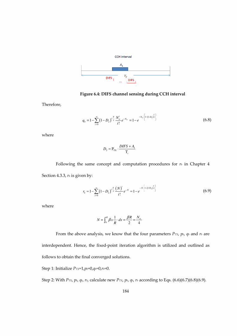
184

Figure 6.4: DIFS channel sensing during CCH interval

Therefore,

( )( )21 1-

2

0

1 1 1!

T

tr

tr

i N DTi Ntr

b

i

Nq D e e

i

τ

τ

∞ − ⋅ − ⋅ −

=

= − − = −∑ (6.8)

where

1

2 TXPT

c

DIFS AD

+= ⋅

Following the same concept and computation procedures for rb in Chapter 4

Section 4.3.3, rb is given by:

( )( ) ( )21 1-D

2

0

1 1 1!

TiNT

i N

b

i

Nr D e e

i

τ

τ

∞ − ⋅ − ⋅ −

=

= − − = −∑

(6.9)

where

0

1

2 4

Rtr

NRN x dx

R

ββ= ⋅ = =∫

From the above analysis, we know that the four parameters PTX, pb, qb and rb are

interdependent. Hence, the fixed-point iteration algorithm is utilized and outlined as

follows to obtain the final converged solutions.

Step 1: Initialize PTX=1,pb=0,qb=0,rb=0.

Step 2: With PTX, pb, qb, rb, calculate new PTX, pb, qb, rb according to Eqs. (6.6)(6.7)(6.8)(6.9).

185

Step 3: If PTX, pb, qb, rb converge with the previous values, then stop the algorithm;

otherwise, go to step 2 with the updated PTX, pb, qb, rb. Once the parameters PTX, pb, qb, rb

are determined using the above algorithm, they are used for both MAC and application

layer performance indices computation in the next section.

6.4 Performance Metrics



The mean transmission delay conditioning on a BSM arrives at t0 is given by:

( )0

01

cT t

TAF t dt

−

− ∫

Therefore, the un-conditioning mean transmission delay for a BSM is:

[ ] ( )( )0

00 0

11

c cT T t

TA

c

E D F t dt dtT

−

= − ∫ ∫

(6.10)

6.4.1.2 Node Reception Probability (NRP)

In Chapter 3, the reliability for a packet transmission (node reception probability,

packet delivery ratio and packet reception ratio) has not taken into account of channel

fading effects. In this Chapter, to model real traffic scenarios, we consider hidden

terminal problem, concurrent transmissions and channel fading with path loss to obtain

MAC layer packet transmission reliability metrics.

As shown in Fig. 4.7, we compute the node reception probability Ps(x) that node

U successfully receives the broadcast BSM from the tagged node O. Three factors

186

affecting the performance of the packet reception are considered: hidden terminal

problems, collision due to concurrent transmissions, and channel fading.

a. Impact of hidden terminals

Based on the SMPA model and its solution, we have the probability that node

U’s reception of the broadcast message from node O is free from the hidden terminals:

1TX

1

21 1-P

T1

TX

0 1

2 ( )( ) (1 P )

T !

T

c

Ax

T i Aix

H

i c

A xP x e e

A i

τβ

βτβ

⋅

− − ⋅ ∞ − ⋅ −

=

⋅= − ⋅ =

−∑ (6.11)

b. Impact of concurrent collisions

In addition to collisions caused by the hidden nodes, transmissions from nodes

within interference range from the tagged node in the meantime at which the tagged

node transmits may also cause collisions. If the tagged node has not gone through the

backoff process before transmitting the packet, concurrent transmission will not occur

(with probability 1-qb). Otherwise, the packet transmission is synchronized to the

beginning of a slot time and concurrent transmission may occur if other vehicles’

transmission is also synchronized by the backoff process.

Given that as both O and U sense the channel idle, O will transmit within the

duration of a slot. Suppose O has experienced backoff process. In order to prevent

interference from concurrent collisions with U’s receiving the broadcast message sent by

O, no transmission in [-(R-x), R] is allowed. The average number of nodes transmitting

in the concurrent slot in area [0, x] is βxPTX·σ/(Tc-A1)·T/τ. Suppose node W is y away from

187

O, x<y<R. The probability that node W starts transmitting during the slot is the

probability that node W intends to transmit and all nodes in [R+x, R+y] are not in

transmitting state, which is expressed as:

3( ) 1 (1 )

( )

1 3 1

0

( ( ))( , ) (1 ) =

!

T

y x DT ii

y x

s

i

T y x TP y x D D e D e

i

τββτ

β

τ τ

− − − −∞ ⋅ − −

=

−= ⋅ − ⋅∑

(6.12)

where

1

3 TX

1

PT

c

AD

A= ⋅

−

Hence, the average number of nodes that start transmission during the slot that

collides with the transmission from O is:

3 3( ) 1 (1 ) ( ) 1 (1 )1

1

3

( , ) 1

1 (1 )

T T

y x D R x DR R

S s Tx x

TD

Tn P y x dy D e dy e

D

τ τβ β

τ

τβ βτ

− − − − − − − −

⋅

= = ⋅ = − − −

∫ ∫

(6.13)

Suppose node V is |z| away from O, -(R-x)<z<0, the probability that the node V

starts transmitting during the slot is the probability that node V intends to transmit and

all nodes in [z-R, -R] are not in transmitting state, which is expressed as

( )31 1

1 3 1

0

( )'( , ) (1 )

!

TiT z Di

z

s

i

zT TP z x D D e D e

i

τββτ

β

τ τ

∞ − − − ⋅ −

=

= ⋅ − = ⋅∑

(6.14)

Therefore, the average number of nodes that start transmission during the slot

that collides with the transmission from O is:

( )

( )

( )( )

( )3 31 1 ( ) 1 110 0

1

3

'( , ) 1

1 1

T T

z D R x D

T s TR x R x

TD

Tn P z x dz D e dz e

D

τ τβ β

τ

τβ βτ

− − − − − − −

− − − −

⋅

= = ⋅ = − − −

∫ ∫

(6.15)

188

Hence, the total average number of nodes that may transmit concurrently is:

1s T

Tn n n x Dβ

τ∑ = + + ⋅ ⋅

(6.16)

Therefore, given Poisson node distribution, the probability that no nodes within the

reception range of U start transmission during the slot that collides with the


( ) ( )0( )

( ) exp( ) 1 exp( ) 10!

con b b b b

nP x q n q q n q∑

∑ ∑

= ⋅ − + − = ⋅ − + −

(6.17)

c. Impact of channel fading with path loss

DSRC channel modeling involves two important aspects: large scale path loss

and small scale fading. The former is used to determine the average received signal

strength at a particular distance from the transmitter, whereas small scale fading

generally involves the detailed modeling of multi-path fading statistics, power delay

profile, and Doppler spectrum. The Nakagami distribution has been shown to fit the

amplitude envelope of empirical data for DSRC channel well. The probability density

function (PDF) of a signal amplitude Y in Nakagami fading can be expressed as:

2 1 22( ) exp( ), 0, 0, 1 / 2

( )

m m

Y m

m y myf y y m

mω

ωω

−

= − ≥ > ≥Γ

(6.18)

where m is the fading parameter, and ω is the average received power. The values of the

two parameters are functions of distance to the sender. From empirical data obtained for

vehicular environment in [40], the fading parameter m is approximated as 3 for low

189

values of d (d<50m) expecting line of sight conditions, 1.5 for middle range distances

(50m≤d≤150m), and 1 (Rayleigh distribution) for distance higher than 150m.

The path loss model is represented by the following equation:

0

0

( )( )

( )

x x

x x

γω

ω=

(6.19)

where ω(x0) and ω(x) are the mean received power with distance to the sender x0 and x,

respectively, and γ is the path loss exponent. γ is usually empirically determined by

field measurement. γ can be 2 for free space environment, 1.6~1.8 for indoor line of sight,

and 2.7~5 for obstructed area or shadowed urban area. In this work, we use 2 as the

value for γ.

According to PDF for signal amplitude Y, the PDF of the signal power Z=Y2 is:

1 ( / )( )

( )

mm mz

Z m

mf z z e

m

ω

ω− −=

Γ (6.20)

Therefore, the CDF of the signal power Z is:

1 ( / )

0( )

( )

mz

m m x

Z m

mF z x e dx

m

ω

ω− −=

Γ ∫

(6.21)

Then, the probability that a message is successfully received in the absence of

interferers deduces from the probability that the message’s signal power is stronger than

the power reception threshold pth, that is:

1 ( / )

0

( ) 1 ( )

1( )

th

F Z th Z th

mp

m m x

m

P P Z p F p

mu e du

m

ω

ω− −

= > = −

= −Γ ∫

(6.22)

190

pth should, in average, be detected in a distance equal to the “intended” communication

range R from the transmitter.

( )

( ) ( )

thp R x

x x R

γω

ω ω

= =

(6.23)

Therefore:

R( )

thx p

x

γ

ω

=

(6.24)

Hence, we obtain the expected probability of successfully receiving a message at

distance x:

( )

( )

1 ( / )

0

1/1

0

1( )

1( )

th

mp

m m u

F m

m

Rm x mu

mP x u e du

m

x mu e du

m

γγ

ω

γ

ω− −

− −

= −Γ

= −Γ

∫

∫

(6.25)

Taking hidden terminal, possible packet collisions, and channel fading and path

loss into account, the probability (or node reception probability) that the node U receives

the broadcast message from the tagged node O is:

( ) ( ) ( ) ( )s H con F

P x P x P x P x= (6.26)

6.4.1.3 Packet Reception Ratio (PRR)

PRR over a coverage range with distance x is defined as, considering vehicles

within the coverage range, the percentage of nodes that successfully receive a packet

from the tagged node among all the receivers that are at the moment that the packet is

sent out.

191

Assuming Poisson distribution of nodes along a 1-D line, the average number of

nodes within an incremental distance dx should be βdx. Given the reception probability

of each node Ps(x), the average number of nodes in dx that successfully receive the

broadcast message from the tagged node is Ps(x)βdx. For a coverage distance with range

R from node O, PRR over a coverage range with distance x (0<x≤R) found by integrating

the probabilities that nodes with distance x to the source node O within an incremental

range successfully receives the broadcast message from O. Therefore,

0

0

( ) 1( ) ( ) ;

x

xs

s

P u duPRR x P u du x R

x x

β

β= = ≤∫

∫

(6.27)

6.4.1.4 Packet Delivery Ratio (PDR)

PDR over a coverage range with distance x is defined as the probability that a

broadcast packet from the tagged vehicle is successfully received by all vehicles within

the coverage range. We need to derive PDR with respect to two aspects: the impact from

concurrent transmission and hidden terminal problem together and the impact from

channel fading.

a. Impact of hidden terminals and concurrent transmissions

Suppose there is no influence from channel fading, then only concurrent

transmission and hidden terminals problem will lead to packet reception failure.

Suppose there are n1 vehicles locate on the left hand side of the tagged vehicle and n2

vehicles locate on the right hand side within distance x. Then, if both the left most

192

vehicle and right most vehicle have successfully receive the packet from the tagged

vehicle, then all vehicles within coverage range x of the tagged vehicle will successfully

receive the packet. This is because both the left most vehicle and right most vehicle

successfully receive the packet ensures that there is no concurrent transmission and

hidden terminals’ influence for all vehicles between them.

Let’s consider vehicles on one hand side (left) of the tagged vehicle first. Given

that there are n vehicles located on one hand side of the tagged vehicle within the

coverage range x, the conditional joint pdf of the n vehicles’ locations Y1, Y2, …, Yn is

given by [9]:

( )1 2 1 2

!, , , | , 0

n nn

nf y y y N x n y y y x

x= = ≤ ≤ ≤ ≤ ≤ L L (6.28)

Therefore, the probability that the left most vehicle within coverage area x of the tagged

vehicle receive the packet successfully is:

( ) ( ) ( ) ( ){ } ( )( )

( ) ( )( )

( )

3 4 2 3 1 2

3 2 1

3 4 2 3 1 2

3 2 1

1 1 2 1 2 30 0 0 0

0

1 2 30 0 0 0

0

, , , |

!

!

n

n

n

n

y x y y y y y y

con n H n n ny y y y

n

ny x y y y y y y

x

con n H n nny y y yn

con n H

PDR x P y P y f y y y N x n dy dy dy dy P N x n

xnP y P y dy dy dy dy e

x n

P y P

ββ

∞ = = = =

= = = ==

∞ = = = =−

= = = ==

= = ⋅ =

= ⋅ ⋅ ⋅

=

∑ ∫ ∫ ∫ ∫

∑ ∫ ∫ ∫ ∫

L L L

L L

( )( )

( ) ( ){ } ( )

( ) ( ) ( ){ } ( )

1

00

1

00

1

00

!

1 !

1 !

n

n

n

n

n

n

nny x

xn

n nnyn

ny x

n x

con n H n n ny

n

y x n x

con n H n n ny

n

xn yy dy e

x n

P y P y y dy en

P y P y y dy en

β

β

β

β

β

ββ

−∞ =−

==

∞ =− −

==

∞ = − −

==

⋅⋅ ⋅ ⋅

= ⋅ ⋅ ⋅−

= ⋅ ⋅ ⋅−

∑ ∫

∑ ∫

∑ ∫

(6.29)

b. Impact of channel fading with path loss

For channel fading’s impact, we can assume impact of fading on different nodes

is independent from each other. Hence,

193

( ) ( ) ( ) ( )( )

( )( )

3 4 2 3 1 2

3 2 1

3 4 2 3 1 2

3 2 1

2 1 2 1 2 30 0 0 0

0 1

1 2 30 0 0 0

1

, , , |

!

!

n

n

n

n

ny x y y y y y y

F i n ny y y y

n i

nn

y x y y y y y y

F i nny y y yi

PDR x P y f y y y N x n dy dy dy dy P N x n

xnP y dy dy dy dy e

x n

β

∞ = = = =

= = = == =

= = = =−

= = = ==

= = ⋅ =

= ⋅ ⋅ ⋅

∑ ∏∫ ∫ ∫ ∫

∏∫ ∫ ∫ ∫

L L L

L L

( )( )

( )

3 4 2 3 1 2

3 2 1

3 4 2 3 1 2

3 2 1

0

1 2 30 0 0 0

0 1

1 2 30 0 0 0

0 1

!

!

n

n

n

n

x

n

nn

y x y y y y y yx

F i n ny y y yn i

ny x y y y y y y

n x

F i ny y y y

n i

xnP y dy dy dy dy e

x n

P y dy dy dy dy e

β

β

β

β

β

∞

=

∞ = = = =−

= = = == =

∞ = = = =−

= = = == =

= ⋅ ⋅ ⋅

= ⋅ ⋅ ⋅

∑

∑ ∏∫ ∫ ∫ ∫

∑ ∏∫ ∫ ∫ ∫

L L

L L

(6.30)

Therefore, taking into consideration of hidden terminal problem, concurrent

transmissions and channel fading with path loss for vehicles on both sides of the tagged

vehicle, packet delivery ratio is given by:

( ) ( ) ( )2

1 2PDR x PDR x PDR x= ⋅ (6.31)

6.4.2 Application-level Performance Metrics

6.4.2.1 Application-level Delay

Application-level delay is the duration between the time when a broadcast

packet is generated at application layer of transmitting vehicle and the time at which the

first successful packet is received by the application layer of receiving vehicle:

[ ] ( )1

1

1( ) ( 1) [ ] ( ) 1 ( ) [ ] 1

( )

i

D s s

i s

E T i E D P x P x E DP x

τ τ∞

−

=

= − + − = + −

∑

(6.32)

where x is the distance between the sender and receiver, E[D] is the MAC-level mean

transmission delay of the BSM given by Eq. (6.10) and Ps(x) is the node reception

probability given in Eq. (6.26).

194

6.4.2.2 T-window Reliability

Application-level T-window reliability is defined [53] in the probability of

successfully receiving at least one packet out of multiple packets from a broadcast

vehicle at distance x, within a given time Ttol (referred to as application tolerance

window):

( , ) 1 (1 ( ))tolT

app tol sP x T P x τ= − −

(6.33)

where τ is the beacon generation interval and Ps(x) is the node reception probability

given in Eq. (6.26).

6.4.2.3 Awareness Probability

The awareness probability [54] is the probability of successfully receiving at least

n packets in the tolerance time window T.

( , ) ( ) (1 ( ))

tol

tol

T

Ttolk

k

A s s

k n

T

P x n P x P x

k

τττ

−

=

= −

∑

(6.34)

It is noted that the awareness probability PA(x, n) becomes the application-level T-

window Reliability Papp(x, Ttol) as n is equal to 1.

6.4.2.4 Average Number of Invisible Neighbors

The average number of invisible neighbor problem has been defined and

described in detail in Section 4.4.2.5 in Chapter 4. Using the same concept, we have:

0 0

1( ) 2 (1 ( )) 2 1 ( , ) 2 2 ( , )

x x

invisible app tol app tolN x x PRR x x P s T ds x P s T ds

xβ β β β

= − = − ⋅ = −

∫ ∫

(6.35)

195


6.5.1 Simulation Description

The simulator used in this work is NS2 release version 2.35. Channel switching

mechanism is not incorporated in this version; therefore, the NS2 source codes are

modified to implement the channel switching behavior. We intend to evaluate the

performance for broadcast BSM messages in the CCH while the radio is participating in

IEEE 1609.4 compliant channel switching activities. Hence, based on the strategy in [61],

the message generation frequency is adjusted to 100/(46·τ), and the messages generated

during non-CCH intervals are ignored and not been broadcasted. In addition,

unfinished packet receptions will be dropped when the CCH interval expires. This is

implemented in PHY layer by setting an error flag for the MAC to declare CRC check

failure.

6.5.2 Numerical Results

Table 6.1: Input parameter settings


Transmission range R 500 m CCH interval Tc 46 ms

Slot time σ 16 us Data rate Rd 24 Mbps

DIFS 64 us Packet length PL 100 bytes

CW W-1 15 path loss exponent ϒ 2

PHY preamble TH1 40 µs

Fading Parameter m 3 for d<50m 1.5 for 50m≤d<150m 1 for d≥150m

MAC header TH2 272 bits

PLCP header TH3 4 µs Sync period T 100 ms

196

The MAC-level mean transmission delay under various network parameters is

presented in Fig. 6.5 using parameters shown in Table 6.1. The time to transmit the

header is: TH= TH1+TH3/Rd+TH3.

Fig. 6.5 shows that the MAC-level mean transmission delay matches very well

with the simulation results under various vehicle density β (#vehicles/m) and message

generation interval τ (s), which verified the accuracy of our proposed model. In

addition, the MAC-level mean transmission delay is relatively small since the maximum

delay is still less than 0.3 ms under typical network parameters that we choose.

0.02 0.04 0.06 0.08 0.1 0.12 0.14 0.16 0.18 0.2

1.4

1.6

1.8

2

2.2

2.4

2.6

2.8

3x 10

-4

Density (#vehicles/m)

MA

C-level m

ean t

ransm

issio

n d

ela

y

tau=1 analytic

tau=1/3 analytic

tau=1/5 analytic

tau=1/7 analytic

tau=1 sim

tau=1/3 sim

tau=1/5 sim

tau=1/7 sim

Figure 6.5: MAC-level mean transmission delay

197

0 50 100 150 200 250 300 350 400 450 5000

0.1

0.2

0.3

0.4

0.5

0.6

0.7

0.8

0.9

1

Distance (m)

Pro

babili

ty

PDR analytic

PDR sim 99% CI

NRP analytic

NRP sim 99% CI

PRR analytic

PRR sim 99% CI

Figure 6.6: Packet transmission reliability

The other MAC-level performance indices except the mean transmission delay

are functions of distance from the sender to receiver. Hence, we evaluate them according

to distance under a specific vehicle density and message generation interval setting

(β=0.1 vehicles/m and τ=1/7 s). The analytic-numerical results for NRP, PRR and PDR are

obtained and compared with simulation results as shown in Fig. 6.6. We conducted 50

runs of simulation with each run lasting 1 second. Due to the Central Limit Theorem,

99% confidence intervals (CI) are computed based on normal distribution. The time

taken to obtain such analytic-numerical results for NRP, PRR and PDR is around 5

minutes, whereas the simulation takes several hours to obtain the corresponding 99% CI.

The results in Fig. 6.6 show that NRP has a good match with the simulation results, and

the relative difference becomes smaller when the distance from the sender is longer.

Analytic result for PRR is relatively higher than the simulation results with acceptable

198

accuracy. Such difference may result from the fact that the NRP for shorter distance is a

little higher than the simulation results and PRR(x) is derived from the integration of

NRP over the range [0, x]. The result for PDR shows that PDR has a very good match

with the simulation results when the distance from the sender is longer than 150 m,

while the difference is relatively obvious when the distance is shorter than 150 m. This

may also result from the fact that analytic model for PDR is derived from NRP which

has bigger difference with the simulation results when the distance is shorter. In

addition, due to the computational complexity for Eq. (6.30), we used polynomial

approximation to approach the analytic results for PF(yi), which has relatively larger

difference with the exact analytic-numerical results when the distance is short. To sum

up, the analytic models for MAC-level performance metrics have a good match with

simulations with acceptable differences for shorter distances, which validate the

accuracy of our model.

Moreover, we observe that as the distance becomes longer, the NRP, PRR and

PDR decrease. For NRP, when the distance from the sender is longer, a receiver has

lower probability to receive a broadcast packet resulting from the impact of concurrent

transmission, hidden terminal problems and channel fading with path loss. Due to this

fact, the percentage of receivers that successfully receive the packet over all receivers in

the coverage area (PRR) also decreases as the coverage area becomes larger. For PDR,

which represents the probability that all vehicles within a coverage area receive a

199

broadcast packet successfully, decreases dramatically with the distance. Fig. 6.6 shows

that PDR drops to almost 0 when the coverage area is a half of the communication

range.

0 50 100 150 200 250 300 350 400 450 5000.4

0.5

0.6

0.7

0.8

0.9

1

Distance (m)

Pro

babili

ty

PA(n=1) analytic

PA(n=2) analytic

PA(n=3) analytic

PA(n=1) sim 99% CI

PA(n=2) sim 99% CI

PA(n=3) sim 99% CI

Figure 6.7: Awareness probability with different packet requirements

0 50 100 150 200 250 300 350 400 450 5000

0.05

0.1

0.15

0.2

0.25

0.3

0.35

Distance (m)

Applic

ation layer

dela

y (

s)

analytic

sim 99% CI

Figure 6.8: Application-level delay

200

0 50 100 150 200 250 300 350 400 450 5000

0.1

0.2

0.3

0.4

0.5

0.6

0.7

0.8

0.9

1

Distance (m)

No.

of

invis

ible

neig

hbors

analytic

sim 99% CI

Figure 6.9: Average no. of invisible neighbors

Figs. 6.7-6.9 show the comparisons between analytic model and simulation for

application-level performance and reliability metrics with tolerance window Ttol=1s. The

results show that they have very good match over the whole communication range. In

addition, we observe that the differences with simulation results when the distance is

shorter for MAC-level performance and reliability metrics (NRP, PRR and PDR) have

little impact on the accuracy of the application-level metrics. Therefore, this further

validates the accuracy ofour proposed model for application-level performance and

reliability metrics. Furthermore, Figs. 6.7-6.9 show that the application-level metrics

varies dramatically when the distance from the sender is longer. T-window reliability

and awareness probability decreases with the distance (Notice that T-window reliability

is equivalent to the awareness probability with packet requirement n=1). In addition, we

observe from Fig. 6.7 that as the packet requirement increases, the awareness probability

decreases faster. Fig. 6.8 shows that the application-level delay increases faster with the

201

distance and is much higher than the MAC-level mean transmission delay in Fig. 6.6.

Fig. 6.9 shows that the average number of invisible neighbors increases dramatically

with the distance especially when the distance is longer.

6.5.3 Impacts of Channel Switching and Channel Fading

In our previous work in Chapter 2 and 3, we have shown that hidden terminal

problem has much larger impact than concurrent transmission on packet reception

probability (PDR and PRR). In this work, we have incorporated channel fading scenario.

Hence, we will evaluate the impact of channel fading on the packet reception

probabilities in this section. Channel fading has no impact on MAC-level mean

transmission delay since we only account for the packets that have been successfully

received. Other MAC-level and application-level performance metrics are derived based

on NRP, and hence it is only necessary to evaluate the impact of channel fading on NRP.

An analytic model is proposed and validated in Chapter 4 [68] for periodic beacon

message broadcast over a single channel without considering channel switching

mechanism and channel fading. Hence, to evaluate the influence of channel switching

mechanism, we compare the models in Chapter 4 [68] to our newly models in this

chapter. The message generation interval is set to be the same for these two models. The

difference is that: the model in Chapter 4 [68] periodically broadcasts these messages,

whereas the new model schedules the messages to be broadcast only during CCH

intervals using optimized scheduling [61][94].

202

0 50 100 150 200 250 300 350 400 450 5000

0.1

0.2

0.3

0.4

0.5

0.6

0.7

0.8

0.9

1

Distance (m)

NR

P

w/o CHSW w/o fading

w/ CHSW w/o fading

w/ CHSW w/ fading

Figure 6.10: Impacts of channel switching and channel fading on NRP

Fig. 6.10 shows the analytic-numerical results for NRP under different scenarios:

without channel switching and without channel fading (based on results from [68],

referred as “w/o CHSW w/o fading”), with channel switching and without channel

fading (exclude channel fading influence in Eq. (6.26), referred as “w/ CHSW w/o

fading”), with channel switching and with channel fading (Eq. (6.26), referred as “w/

CHSW w/ fading”).

We observe that incorporating channel switching mechanism degrades NRP

linearly compared to non-channel switching mechanism. Such phenomena results from

the fact that for the same number of packets generated, non-channel switching

mechanism allocates packets to be transmitted over the whole time period, while

channel switching mechanism schedules all packets transmitted CCH intervals only.

Therefore, channel switching mechanism has more collisions in CCH intervals, which

203

leads to lower NRP. In addition, NRP under channel fading scenario is much lower than

that without channel fading. Such difference becomes more obvious when the distance

from the sender is longer. When the distance is less than 150 m, the difference is

relatively small because the fading parameter m we used is larger for small distances.

Therefore, we conclude that bigger fading parameter brings smaller fading to the

communications, whereas smaller fading parameter has significant impact on degrading

the NRP.

6.6 Conclusions

In this chapter, an analytic model is proposed to characterize the BSM message

broadcasting in CCH interval for multi-channel operations. Optimized scheduling is

assumed to avoid synchronization collisions presented in basic access mode for IEEE

802.11p and IEEE 1609.4. Channel fading with path loss is taken into account in this

work to capture practical communication environment. MAC-level performance indices

including mean transmission delay, NRP, PDR, PRR and application-level performance

including T-window reliability, awareness probability, application-level delay and

average number of invisible neighbors are derived. Simulation in NS2 incorporating

channel switching mechanism is implemented for verification purposes. The good

match between the analytic model and simulation results validate the accuracy of our

proposed model.

204

In future, vehicle mobility will be considered to make the model more realistic.

Even though it has been proven in [41][42] that high mobility of vehicles has very minor

impact on the performance of the direct message broadcasting with high data rate, it

may have great impact on application level performance metrics.

205

7. Multi-hop Dissemination Evaluation

7.1 Motivation

In the U.S., Dedicated Short Range Communication (DSRC) [1][45] spectrum

consists of seven channels as shown in Fig. 1.1 to support both safety and non-safety

applications in vehicular ad hoc networks (VANET). Channel 178 is the control channel

(CCH), which is the default channel for safety communication. Periodic beacon message

containing vehicle status information (e.g., position, speed, direction) may be

transmitted through this channel to enable various collision avoidance applications. In

dense traffic scenarios, the periodic beacons may consume the entire channel

bandwidth. Therefore, Channel 172 at one edge is preserved for low-latency, high

availability vehicle to vehicle (V2V) critical safety communications. The event-driven

safety message, which is broadcast in case of an emergency situation (e.g., accidents,

hard-braking, road hazard), is a type of safety critical message that is most likely to be

transmitted through such a channel.

The one-hop direct message broadcasting can cover a short range due to radio’s

limited communication range (usually less than 1 km in DSRC). However, some event-

driven safety applications may be required to cover longer distances than the

communication range, such as in the post-crash notification or road hazard warning

situations. Therefore, multi-hop message dissemination is necessary in such scenarios.

For multi-hop broadcast scheme, the protocols proposed in the literature can be

206

categorized into several classes [80]: simple flooding, probability-based methods, area-

based methods and neighbor knowledge method. Many techniques focus on minimizing

the number of retransmissions while attempting to ensure that a broadcast packet is

delivered to every vehicle within the intended coverage area. In this chapter, we adopt a

robust relay selection strategy proposed in our previous work [73] for multi-hop

propagation of event-driven safety message utilizing distance-based timers to choose

farthest node as the relay.

Most of the previous work on this topic is based on simulations [98][99][100][101]

to analyze the performance and reliability of multi-hop message dissemination. Several

experimental studies [102][103][96] have been conducted to capture more practical

network dynamics. Very few analytic models [73] have been proposed. However, many

of the existing studies [73][98] assume a fixed one-hop message transmission reliability:

when a vehicle broadcasts a message, all vehicles within the transmission range from the

sender have the same probability of correctly receiving the message. Such an

assumption fails to capture complex traffic scenarios such as fading channel, Doppler

spectrum effect, etc. In addition, the simulation approach usually consumes long time

and only a few metrics can be obtained within a reasonable length of time. Due to the

high equipment cost, the experimental testbed usually only consists of very few vehicles

(six in [102], and four in [103][96]). Even though some techniques are utilized to create a

207

large scale virtual communication network using a small number of vehicles, the

resulting virtual network is still only capable of capturing sparse network scenarios.

In this chapter, we propose an accurate and efficient analytic model to evaluate

the performance and reliability of multi-hop safety message dissemination. Since event-

driven safety message is occasionally generated (only when an emergency event is

detected), we can reasonably assume that during the lifetime of an event-driven safety

message, no other event-driven safety message is generated. In other words, we

concentrate on the performance and reliability of multi-hop delivery of a single event-

driven safety message. Therefore, concurrent transmissions and hidden terminal

problem do not exist in such a system that is under consideration. The main focus of this

chapter is the impact of channel fading on the system performance and reliability.

The main contributions of this chapter are: 1) An accurate and efficient analytic

model is developed to capture the channel fading’s effect on multi-hop safety message

dissemination; 2) Various performance and reliability metrics are derived to provide a

deeper understanding of the message transmission behavior from different angles. 3)

Extensive simulations are conducted to verify the accuracy of our proposed models.

This chapter is organized as follows. Section 7.2 briefly explains the system

under investigation and model assumptions. Section 7.3 presents analytic models to

evaluate various types of performance and reliability metrics. Analytic-numerical results

are shown in Section 7.4 to compare with simulations. Section 7.5 shows the

208

simplification techniques for the analytic models proposed. Conclusions are in the last

section.

7.2 System Description and Assumptions

Once an emergency message is generated, its header contains the information

about the originating source node, the type of message and the message propagation

direction. Based on this information, we propose and evaluate an efficient multi-hop

broadcast scheme for the emergency notification services. We adopt a multi-hop relay

scheme similar to the one proposed in our previous paper [73], which provides a reliable

way to select a routing node to rebroadcast the emergency message. A vehicle will be

selected to rebroadcast the message under the following conditions:

• the vehicle has successfully received the message;

• the vehicle’s distance to the sender is the farthest among all one-hop vehicles that

have received the message successfully.

The second condition is guaranteed by setting a deterministic timer in each

vehicle that received the message. The timer is a function of the distance from the

receiver to the sender x and is defined as follows:

( )max 1

0

AD

xT if x R

Rt x

if x R

− ≤

= >

(7.1)

where Tmax is chosen as the one-hop lifetime of the emergency message and R is the

average transmission range of a node.

209

All vehicles that received the message will trigger the AD timer according to Eq.

(7.1). The one whose AD timer expires first is chosen to rebroadcast the emergency

message. If such rebroadcast message is received by some vehicles in the hop, they will

cancel their AD timers and stop their attempts to relay the message. In case that the

rebroadcast message from the selected node fails to reach some nodes in the hop due to

fading channel condition, those candidate nodes keep counting down their AD timer

until one of the candidates is selected as a new relaying node. This process continues

until at least one rebroadcast is successful in the hop.

The proposed multi-hop scheme aims at a fast and reliable delivery of the

emergency message. The AD timer strategy guarantees that the farthest node in the

transmission direction has the highest priority to be selected as the relaying node so that

the multi-hop coverage can be extended farthest as fast as possible. In addition, to

achieve reliable delivery, the redundant relaying nodes are set in a ready mode through

the distance based counters to cope with possible delivery failures of the rebroadcast

message in the one hop.

The following assumptions are made in this chapter to produce a simplified yet

high fidelity analytic model. The network is considered one-dimensional (1-D). The

number of vehicles in a line is Poisson distributed with parameter λ (vehicle density). In

addition, all vehicles are assumed to have the same transmission range, receiving range,

and carrier sensing range R. Vehicle mobility is not taken into account in this chapter.

210

The 1-D VANET model is a good approximation of ad hoc networks on highway when

the distances between lanes on the highway are negligible compared with the length of

the highway. Furthermore, recent statistical analysis of empirical data collected from

real-world scenarios [34][35] show that Poisson model is a good fit for sparse highway

vehicle traffic in terms of inter vehicle distance. Heavy traffic scenarios where

exponentially distributed inter vehicle distance does not fit will be considered in our

future work. We have set the values of three communication ranges (transmission range,

receiving range and carrier sensing range) the same to simplify the analysis. Extension

of the model to more general cases with different values of communication ranges is

straightforward [36].

7.3 Analytic Models

7.3.1 Channel Fading Model

In this chapter, we concentrate on the impact of channel fading on multi-hop

safety message transmission. DSRC channel modeling involves two important aspects:

large scale path loss and small scale fading. The former is used to determine the average

received signal strength at a particular distance from the transmitter, whereas small

scale fading generally involves the detailed modeling of multi-path fading statistics,

power delay profile, and Doppler spectrum. The Nakagami distribution has been shown

to fit the amplitude envelope of empirical data for DSRC channel well [94]. The

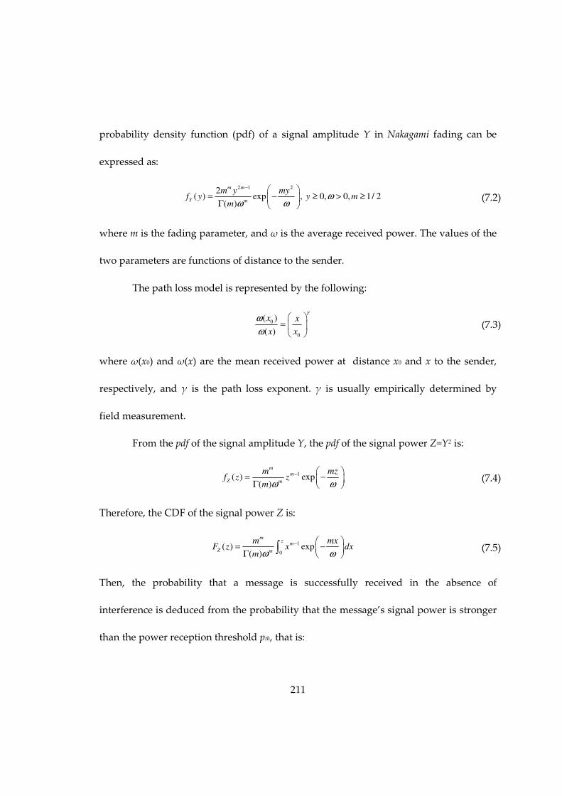
211

probability density function (pdf) of a signal amplitude Y in Nakagami fading can be

expressed as:

2 1 22

( ) exp , 0, 0, 1/ 2( )

m m

Y m

m y myf y y m

mω

ωω

− = − ≥ > ≥

Γ (7.2)

where m is the fading parameter, and ω is the average received power. The values of the

two parameters are functions of distance to the sender.

The path loss model is represented by the following:

0

0

( )

( )

x x

x x

γω

ω

=

(7.3)

where ω(x0) and ω(x) are the mean received power at distance x0 and x to the sender,

respectively, and γ is the path loss exponent. γ is usually empirically determined by

field measurement.

From the pdf of the signal amplitude Y, the pdf of the signal power Z=Y2 is:

1( ) exp

( )

mm

Z m

m mzf z z

m ωω−

= − Γ

(7.4)

Therefore, the CDF of the signal power Z is:

1

0( ) exp

( )

mz

m

Z m

m mxF z x dx

m ωω−

= − Γ

∫

(7.5)

Then, the probability that a message is successfully received in the absence of

interference is deduced from the probability that the message’s signal power is stronger

than the power reception threshold pth, that is:

212

( )

1

0

( ) 1 ( )

1 exp( )

th

s th Z th

mp

m

m

P x P Z p F p

m mxu du

m ωω−

= > = −

= − −

Γ ∫

(7.6)

pth should, on the average, be detected in a distance equal to the intended communication

range R from the transmitter:

( )

( ) ( )

thp R x

x x R

γω

ω ω

= =

(7.7)

Hence, we obtain the probability of successfully receiving a message at a distance x

considering channel fading with path loss effects:

( )

( )

1

0

/1

0

1 exp( )

1 e( )

th

mp

m

s m

mx R

m mz

m muP x u du

m

mz dz

m

γ

ωω−

− −

= − −

Γ

= −Γ

∫

∫

(7.8)

7.3.2 Rebroadcast Probability

Due to the unfavorable characteristics of channel fading in DSRC, various

performance metrics for multi-hop message delivery are impacted. One of the most

important metrics is the rebroadcast probability. In order to better illustrate the

rebroadcast behavior, we evaluate the rebroadcast probability from two perspectives:

one from a broadcast message’s perspective, and another from a receiver’s perspective:

• Message-centric rebroadcast probability Prb is defined as the probability that a

message can be rebroadcast by a receiver within this hop given the message is

broadcast within a hop.

213

• Receiver-centric rebroadcast probability PrbA(x) is defined as given a receiver located

with distance x from the sender, the probability that this receiver can rebroadcast the

safety message.

Figure 7.1: Message rebroadcast in a hop

7.3.2.1 Message-centric rebroadcast probability

As shown in the Fig. 7.1, sender O broadcasts a safety message to all one-hop

receivers. This message can be rebroadcast if at least one one-hop receiver in the

rebroadcast direction receives the message successfully.

Suppose that there are n vehicles located on the rebroadcast direction within O’s

transmission range R. According to Theorem 6.2 in [9], the conditional pdf of the n

nodes’ un-ordered locations T1, T2, …, Tn respectively is given by:

[ ]1

| ( ) , , 1, 2,...,iT i i

f t N R n x t R i nR

= = ≤ ≤ =

(7.9)

We first calculate the conditional probability that a node with location Ti=ti fails

to receive the signal as 1-Ps(ti) and then uncondition by multiplying with the location

density in Eq. (7.9) and integrating to obtain the probability that a single vehicle among

these n nodes fails to receive the message. Next, the probability that none of the one-hop

214

receivers receive the broadcast message successfully is computed as the product of n

single vehicle’s message failure probabilities. Finally, by unconditioning with respect to

the number of nodes N(R)=n, and subtracting from 1, we obtain the probability that at

least one vehicle receives the broadcast message successfully, which is equivalent to the

message-centric rebroadcast probability:

( ) [ ] ( )( )

( )( )

( )

( )( )

( )

0 1 0

0 1 0

0

1

0

1 1 ( ) | ( )

11 1 ( )

!

1 0!

01

!

1

i

i

i

i

i

t Rn

rb s i T i i

n i t

nt R Rn

s i i

n i t

n Rn

n

n

R

n

R I

P P t f t N R n dt P N R n

R eP t dt

R n

eI

n

Ie

n

e

λ

λ

λ

λ λ

λ

λ

λ

=∞

= = =

= −∞

= = =

−∞

=

∞−

=

− +

= − − ⋅ = ⋅ =

= − − ⋅

= − ⋅

= − ⋅

= −

∑ ∏ ∫

∑ ∏ ∫

∑

∑

(7.10)

where

( ) ( )( / )

1

0

( / )1

0

1 ( )( )

( , )( )

t R t R mt R

m mz

s

t x t x

t R mt R

m mz

t x

mI x P t dt z e dz dt

m

mz e dz dt f x m

m

γ

γ

= =− −

= =

=− −

=

= − =

Γ

= ⋅ =

Γ

∫ ∫ ∫

∫ ∫

(7.11)

The f(x,m) in Eq. (7.11) can be significantly simplified to reduce the computational

complexity by changing the order of integration in the double integral. The detailed

simplification is shown in Section 7.5.

7.3.2.2 Receiver-centric rebroadcast probability

Besides the message-centric rebroadcast probability, we are also interested in:

given a receiver located at a distance x from the sender, what is the probability that this

215

receiver will rebroadcast the message? Based on the two conditions for selecting a relay

node in Section 7.2, we know that a vehicle will rebroadcast a message if it successfully

receives the broadcast message from the sender, and all one-hop nodes farther than this

vehicle have not received this message.

Denote a random receiver in the rebroadcast direction to be A, located at a

distance x from the sender O as shown in Fig. 7.1. In addition, assume that there are n

nodes located farther than node A from the sender O but within O’s transmission range

R. According to Theorem 6.2 in [9], the conditional pdf of the n nodes’ un-ordered

locations T1, T2, …, Tn respectively is given by:

[ ]1

| ( ) , , 1, 2,...,iT i i

f t N R x n x t R i nR x

− = = ≤ ≤ =−

(7.12)

Therefore, the rebroadcast probability of node A, conditioned on there being n

one-hop nodes farther than A, can be computed as follows:

• If n=0

( ) ( )1 | ( ) 0rb s

P x N R x P x− = = (7.13)

• If n>0

216

( ) ( ) ( ) [ ]

( ) ( )

( ) ( )

( ) ( )

2

1

1

| ( ) 1 ( ) | ( )

11 ( )

11 ( )

1

i

i

i

i

i

t Rn

rb s s i T i i

i t x

t Rn

s s i i

i t x

n nt R

s s

t x

nn

s

P x N R x n P x P t f t N R x n dt

P x P t dtR x

P x P t dtR x

P x I xR x

=

= =

=

= =

=

=

− = = ⋅ − ⋅ − =

= ⋅ − ⋅

−

= ⋅ − ⋅

−

= ⋅ ⋅

−

∏ ∫

∏ ∫

∫

(7.14)

Therefore, the un-conditioned rebroadcast probability for A (i.e., the rebroadcast

probability for a receiver located at a distance x from the sender) is given by:

( ) ( ) ( ) ( )( )( ) ( )

( ) ( ) ( )

1 2

1 !

n R x

R x

rbA rb rb

n

R x I x

s

R x eP x P x e P x

n

P x e

α

α

α α

α − −∞

− −

=

− − +

− = ⋅ + ⋅

= ⋅

∑ (7.15)

7.3.3 Average Rebroadcast Distance

For multi-hop message dissemination, the number of hops to reach a specific

distance is one of the most important metrics to evaluate how fast a message can be

transmitted. Hence, one-hop rebroadcast distance needs to be analyzed first, based on

which the number of hops to reach a distance can be easily computed.

In Section 7.3.2, the un-ordered statistics for vehicles are considered for both

message-centric and receiver-centric rebroadcast probability calculation, since the

output measures do not depend on the order of vehicles within an area. However, to

assess the rebroadcast distance for a message, we need to pay attention to the ordered

statistics of the receivers because their locations impact the rebroadcast distance.

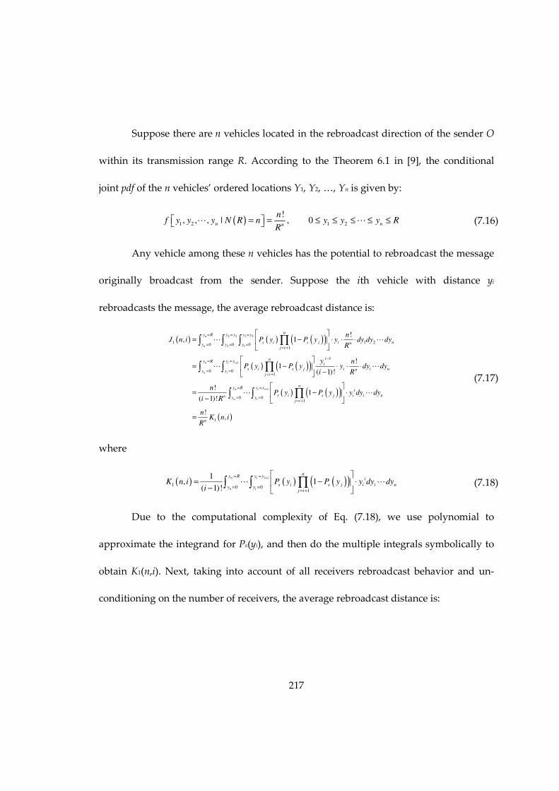
217

Suppose there are n vehicles located in the rebroadcast direction of the sender O

within its transmission range R. According to the Theorem 6.1 in [9], the conditional

joint pdf of the n vehicles’ ordered locations Y1, Y2, …, Yn is given by:

( )1 2 1 2

!, , , | , 0

n nn

nf y y y N R n y y y R

R= = ≤ ≤ ≤ ≤ ≤ L L (7.16)

Any vehicle among these n vehicles has the potential to rebroadcast the message

originally broadcast from the sender. Suppose the ith vehicle with distance yi

rebroadcasts the message, the average rebroadcast distance is:

( ) ( ) ( )( )

( ) ( )( )

( ) ( )( )

2 3 1 2

2 1

1

1 1 20 0 0

1

1

0 01

1

!, 1

!1

( 1)!

!1

( 1)!

n

n

n i i

n i

i

ny R y y y y

s i s j i nny y yj i

iny R y y

i

s i s j i i nny yj i

ni

s i s j i i nn yj i

nJ n i P y P y y dy dy dy

R

y nP y P y y dy dy

i R

nP y P y y dy dy

i R

+

= = =

= = == +

−= =

= == +

== +

= − ⋅ ⋅ ⋅

= − ⋅ ⋅ ⋅

−

= − ⋅

−

∏∫ ∫ ∫

∏∫ ∫

∏

L L

L L

L L

( )

1

0 0

1

!,

n i i

n

y R y y

y

n

nK n i

R

+= =

=

=

∫ ∫

(7.17)

where

( ) ( ) ( )( )1

10 0

1

1, 1

( 1)!

n i i

n i

ny R y y

i

s i s j i i ny y

j i

K n i P y P y y dy dyi

+= =

= == +

= − ⋅

− ∏∫ ∫L L (7.18)

Due to the computational complexity of Eq. (7.18), we use polynomial to

approximate the integrand for Ps(yi), and then do the multiple integrals symbolically to

obtain K1(n,i). Next, taking into account of all receivers rebroadcast behavior and un-

conditioning on the number of receivers, the average rebroadcast distance is:

218

( ) ( )( )

( )( )

( )

1

0 1

1

0 1

1

0 1

,

,!

,

n

rb

n i

nn

R

n i

nn R

n i

D J n i P N R n

RJ n i e

n

K n i e

α

α

α

α

∞

= =

∞−

= =

∞−

= =

= ⋅ =

= ⋅

= ⋅

∑ ∑

∑ ∑

∑ ∑

(7.19)

7.3.4 Average Number of Hops to Reach a Distance

Based on the average rebroadcast distance for a message derived in the previous

section, we can compute the average number of hops to reach a specific distance l for a

broadcast safety message:

( )h

rb

lE l

D

=

(7.20)

7.3.5 Average Rebroadcast Delay

As mentioned in Section 7.1, one-hop receivers that successfully receive the

broadcast message from the sender will trigger their respective distance-based AD

timers before the winner whose timer expires first rebroadcasts the message. Such AD

timer leads to delay in the message rebroadcast process. Hence, in this section, we

evaluate the rebroadcast delay induced by the AD timer. Following an approach similar

to the one in Section 7.3.3 for rebroadcast distance computation, we utilize the ordered

statistics for receivers and obtain the average delay if the ith vehicle with distance yi

rebroadcasts the message given that there are n one-hop receivers:

219

( ) ( ) ( )( ) ( )

( )

2 3 1 2

2 12 1 2

0 0 01

2

!, 1

!,

n

n

ny R y y y y

s i s j AD i nny y yj i

n

nJ n i P y P y t y dy dy dy

R

nK n i

R

= = =

= = == +

= − ⋅ ⋅

=

∏∫ ∫ ∫L L

(7.21)

where

( ) ( ) ( )( )1 1

2 max0 0

1

1, 1 1

( 1)!

n i i

n i

ny R y y

i i

s i s j i i ny y

j i

yK n i P y P y y T dy dy

i R

+= =−

= == +

= − ⋅ ⋅ − ⋅

− ∏∫ ∫L L (7.22)

Considering all receivers rebroadcast behavior and un-conditioning on the number of

receivers, the average rebroadcast delay induced by AD timer for a message is:

( ) ( )( ) ( )2 2

0 1 0 1

, ,n n

n R

AD

n i n i

E J n i P N R n K n i eαα

∞ ∞−

= = = =

= ⋅ = = ⋅

∑ ∑ ∑ ∑ (7.23)

7.3.6 Average Delay to Reach a Distance

The transmission delay for a safety message to reach a specific distance includes

two parts: the time spent to actually transmit the message through the wireless channel,

and the delay induced by the AD timer.

Let T denote the real transmission time for a safety message through a wireless

channel, which is given by:

H

d

PLT T

R= +

(7.24)

In the Eq. (7.24), PL represents the packet length, Rd represents the transmission data

rate, and TH represents the time to transmit the header. For the first hop of message

transmission, the sender needs to sense the channel for DIFS time before it can broadcast

the message to avoid channel collisions. Since we reasonably assume that the safety

220

message occurs occasionally (i.e., when an emergency event presents on the road), the

channel contentions between different safety messages are not considered. Therefore,

the average delay for a safety message to reach distance l is:

( ) ( ) ( )1d h AD

E l DIFS T E l E T= + + − ⋅ + (7.25)

7.3.7 Metrics Related to Message Vanishing

Having been broadcast by a sender for the first time, a safety message may be

rebroadcast several times before it cannot be rebroadcast any further in the rebroadcast

direction (i.e., it vanishes). Several previous papers [96] show interest in evaluating

metrics until a message vanishes from the network:

• What is the total distance travelled by the safety message before it vanishes?

• What is the total number of hops of the message before it vanishes?

• What is the total transmission delay for a message before it vanishes?

Based on the metrics derived earlier in Section 7.3, these metrics can be easily computed.

The average total distance travelled by a message is:

( )

( )

1

1

1

1

1

i

total rb rb rb

i

i

rb rb rb

i

rb rb

rb

D i D P P

D P i P

D P

P

∞

=

∞

=

= ⋅ ⋅ −

= ⋅ − ⋅

⋅=

−

∑

∑

(7.26)

The average total number of hops travelled by a message is:

221

( )1

11

itotal rb

total rb rb

irb rb

D PH i P P

D P

∞

=

= = ⋅ − = −∑

(7.27)

The average total transmission delay for a message is:

( )total total ADE DIFS T H E T= + + ⋅ + (7.28)


To evaluate the accuracy and efficiency of our proposed analytic model, we

compare the analytic-numeric results with the discrete event simulation results

conducted in Matlab. The network parameters are chosen reasonably and most of them

are from real testbeds [96][97], which are listed in Table 7.1. The assumptions made for

the analytic model in Section 7.2 are all made in the simulative solution as well. We

conducted 300 simulation runs. The mean for an output measure is computed for every

10 runs and hence the number of means obtained for each output measure is 30. Due to

the Central Limit Theorem, normal distribution is assumed for these 30 sample means to

compute 99% confidence intervals for the population mean.

Table 7.1: Network parameter


Transmission range R 300 m Packet length PL 300 bytes

DIFS 64 us Tmax 1 second

PHY preamble TH1 40 µs path loss exponent γ 2

MAC header TH2 272 bits Fading Parameter m 3 for d<50m

1.5 for 50m≤d<150 m

1 for d≥150m PLCP header TH3 4 µs

Data rate Rd 6 Mbps

Fig. 7.2 shows the point-to-point node reception probability (NRP) incorporating

channel fading impact and receiver-centric rebroadcast probability (PrbA) with respect to

222

distance from the sender. The lines represent the analytic-numeric results, whereas the

symbols represent the simulation results for 99% confidence interval. In Fig. 7.2, NRP

decreases as distance increases due to channel fading’s effect. In addition, the receiver-

centric rebroadcast probability for a receiver PrbA(x) is nearly zero when the distance is

less than 150m, and it generally increases when the distance approaches the transmission

range R=300m. This is because the rebroadcast vehicle is most likely to be the farthest

one from the sender, which is close to the transmission range. In addition, at the

transmission range point R=300m, we notice that NRP almost equals PrbA. This

observation results from the fact that PrbA is the probability that the vehicle located at R

receives the message (given by NRP) and no farther receivers receive the message. Since

there is no receiver farther than the one located with distance R, the PrbA is equivalent to

NRP for such a vehicle. The good match between the simulation and analytic results

validates the accuracy of our model.

0 50 100 150 200 250 3000

0.1

0.2

0.3

0.4

0.5

0.6

0.7

0.8

0.9

1

Distance (meters)

Pro

babili

ty

NRP

PrbA

NRP sim

PrbA sim

Figure 7.2: NRP and receiver-centric rebroadcast probability

223

0 500 1000 1500 2000 2500 3000 3500 4000 4500 50000

5

10

15

20

25

Distance (meters)

Hops

Average number of hops to reach a distance

real hops

ideal hops

real hops sim

Figure 7.3: Number of hops to reach a distance

0 500 1000 1500 2000 2500 3000 3500 4000 4500 5000-0.5

0

0.5

1

1.5

2

2.5

3

3.5

Distance (meters)

Dela

y (

seconds)

Average transmission delay to reach a distance

delay

delay sim

Figure 7.4: Average transmission delay

Fig. 7.3 shows that as the distance becomes larger, the average number of hops

generally increases. For better comparison, the ideal hop to reach a distance l is also

plotted, which is defined as:

224

_h ideal

lE

R

=

(7.29)

The figure shows that the real number of hops for a message to reach a specific

distance is larger than the ideal hop number. Such difference is more obvious when the

distance is larger. This phenomenon results from the fact that the rebroadcast vehicle is

at a distance less than the transmission range. The simulation results match very well

with our analytic results, which again verifies the correctness of our approach.

Fig. 7.4 shows that when the distance becomes larger, the transmission delay for

a message increases. This increase follows similar pattern as the average number of hops

because the average transmission delay is a linear function of the average number of

hops to reach a specific distance as shown in Eq. (7.25).

The other output measures, which are not distance-based metrics, are listed in

Table 7.2. The average rebroadcast distance is around 254m, which is less than the

transmission range 300m. The average rebroadcast delay is about 0.139s, and this time

accounts for the AD timer delay in the rebroadcast process. Compared to the simulation

results, the analytic results fall within 99% confidence interval of the simulation results.

Hence, this verifies the accuracy of our proposed analytic models. In addition, the

analytic model takes about 1 minute to obtain the numerical results, whereas the

simulation takes 28 minutes. The simulation time will be longer if we need to obtain

tighter confidence intervals. Therefore, our analytic model is much more efficient than

simulations.

225

The message-centric rebroadcast probability for a message is very large because

in the general case, at least one of the receivers can successfully receive the message in

order to rebroadcast it. Since the un-rebroadcast message is an extremely rare event,

which is very difficult to be captured, we have not conducted simulation for such an

output measure. In addition, the average total distance traveled before the message

vanishes is extremely long. As a result, the average total number of hops and the

average total transmission delay are also very high before the message vanishes. In

practice, there could be a lifetime setting for multi-hop broadcast message so that the

rebroadcasting will be terminated if either a destination is reached or the life time

expires.

Table 7.2: Non distance-based metrics

Definitions Symbols Analytic Results Simulation Results 99% CI

Low bound High bound

Average rebroadcast distance (m) Drb 2.54419e+02 2.501e+02 2.631e+02

Average rebroadcast delay (s) EtAD 0.13857762 0.122911 0.166271

Message-centric rebroadcast

probability Prb 0.99999393 -

Average total distance (m) Dtotal 4.196314e+07 -

Average total number of hops Htotal 1.649371e+05 -

Average total transmission delay (s) Etotal 2.293730e+04 -

7.5 Simplification of f(x,m)

This section shows the detailed method to simplify the expression of f(x,m) in Eq.

(7.11) in order to reduce the computation complexity.

Denote:

226

( / )1

00

( , )( )

t d mt R

m mz

t

mh d m z e dz dt

m

γ=− −

=

= Γ ∫ ∫

(7.30)

Therefore,

( / )1

0

( / )1

00

( / )1

00

( , )( )

( )

( )

( , ) ( , )

t R mt R

m mz

t x

t R mt R

m mz

t

t x mt R

m mz

t

mf x m z e dz dt

m

mz e dz dt

m

mz e dz dt

m

h R m h x m

γ

γ

γ

=− −

=

=− −

=

=− −

=

= Γ

= Γ

− Γ

= −

∫ ∫

∫ ∫

∫ ∫

(7.31)

Next, we simplify h(d,m), based on which f(x,m) can be easily simplified. The fading

parameter m in practice can be either modeled as a constant or, more frequently, as a

piecewise function to more precisely capture the real traffic scenarios.

7.5.1 m is a constant over [0, d]

By changing the order of integration in double integral in Eq. (7.30) as shown in

Fig. 7.5, we obtain:

( )( )

1/

( / )1

00

/

1

0

1/

( , )( )

( )

1, ,

( ) ( )

t d mt R

m mz

t

z d Rmd

m mz

R zz

mh d m z e dz dt

m

mdt z e dz

m

d d R dY m m Y m m

m R Rm m

γ

γ

γ

γ γ

γ γ

=− −

=

=

− −

⋅=

= ⋅ Γ

= ⋅Γ

= − ⋅ +

Γ Γ

∫ ∫

∫ ∫ (7.32)

where

( ) 1

0

,

u b

a u

u

Y a b u e du

=− −

=

= ∫

(7.33)

227

represents the lower incomplete Gamma function, which can be easily computed through

built-in functions in software such as Matlab. Let’s denote:

1/

1( , ) , ,

( ) ( )

d d R dg d m Y m m Y m m

m R Rm m

γ γ

γ γ

= − ⋅ +

Γ Γ (7.34)

Hence,

Figure 7.5: Change order of double integral

Figure 7.6: Fading parameter as a piecewise function

228

[ ] 1/

1/

( , ) ( , ) ( , )

( , ) ( , )

1, ,

( ) ( )

1, ,

( ) ( )

f x m h R m h x m

g R m g x m

R RY m m Y m m

m m m

x x R xY m m Y m m

m R Rm m

γ

γ γ

γ

γ

γ

= −

= −

= − ⋅ +

Γ Γ

− + ⋅ +

Γ Γ

(7.35)

7.5.2 m is a piecewise function over [0, d]

Normally, the fading parameter m is a piecewise constant function of

communication distance in most MANET channels, that is:

1

1

for , 1, 2,...

0

i i im m x d x i

x

+= ≤ < =

= (7.36)

where xi are jump points and mi are constant fading parameter values. Through some

mathematic manipulations for h(d,m) in Eq. (7.30), we obtain:

( ) ( ) ( )

{ }

1

2

( , ) , , ,

max :

N

i i i i N

i

i

h d m g x m g x m g d m

N i x d

−=

= − +

= ≤

∑

(7.37)

where g(d,m) is given by Eq. (7.34) and can be easily computed in Matlab. Therefore,

( ) ( )

( ) ( )

1

2

1 2

1

1

( , ) ( , ) ( , )

, ,

, ,

N

i i i i

i N

N N

f x m h R m h x m

g x m g x m

g R m g x m

−= +

= −

= −

+ −

∑

{ }1 max :i

N i x R= ≤

{ }2 max :i

N i x x= ≤

(7.38)

229

7.6 Conclusions

This chapter presents an accurate and efficient analytic model to evaluate the

impact of channel fading on multi-hop safety message disseminations in VANET. We

utilize a distance-based timer to ensure the farthest node from the sender has highest

priority to be chosen to relay the safety message. Various important performance and

reliability metrics are derived and analyzed for thorough understanding of the safety

message transmission behavior. Simulations conducted in Matlab cross validate the

accuracy of our proposed model. In addition, our model is much more efficient in terms

of evaluation time than simulations. The analytic model can also be used to analyze

essential metrics that are difficult to capture in simulations as shown in Table 7.2.

230

8. Two-Dimensional Network Evaluation

8.1 Motivation

Broadcast services are provided widely in various ad hoc network applications

such as safety-related message channels in vehicle-to-vehicle communication, and

military battle field communication [104]. These applications require highly reliable and

real-time communications between mobile nodes under adverse environments.

Broadcast in IEEE 802.11 does not use the virtual carrier sensing and thus only relies on

physical carrier sensing to reduce collisions. Thus, hidden terminal problem in broadcast

VANETs is quite different from that in unicast systems [105]. Normally, the performance

of broadcast VANETs is evaluated by simulations [3] although many analytical models

have been constructed for the performance of IEEE 802.11 based VANETs [106][107]. In

[39][105][41][36], analytical models are proposed to obtain PRR expressions in one-

dimensional (1-D) IEEE 802.11 based broadcast VANETs with hidden terminals.

However, the impact analysis of fading channel model, if any, is approximated by a

constant bit error rate (BER). Assuming spatial Poisson distributed nodes and saturated

packet generation condition, PRR of beacon message broadcast in DSRC VANETs is

investigated in [24] taking into account the impact of Rayleigh fading on IEEE 802.11

based 1-D broadcast VANET. Unfortunately, very few network scenarios in real

applications can be abstracted as 1-D models. However, extension of 1-D VANET

reliability analysis to general 2-D VANET reliability analysis is not trivial because the

231

potential hidden terminal area computation given distribution of nodes in 2-D area is

still claimed to be an open problem [108][109]. For 1-D network, the hidden terminals for

a tagged vehicle are shown in Fig. 8.1. Comparatively, the hidden terminal problem has

more impact on 2-D network since more hidden nodes will exist as shown in Fig. 8.2 for

open field (the area inside the red circle and outside the blue circle will be the hidden

terminal area of the tagged vehicle). Recently, we have conducted PRR analysis in a

special 2-D VANET (two parallel lines approximate two opposite roads on highway)

[105][110]. As of now, there is no work on PRR evaluation in general 2-D IEEE 802.11

broadcast VANETs.

Figure 8.1: Hidden terminals problem for 1-D network

Figure 8.2: Hidden terminals problem for 2-D network

232

Compared with the existing models for performance analysis of broadcast in

VANETs, the main contributions of the proposed analytic model in this chapter are: 1)

general 2-D PRR is analytically derived accounting for IEEE 802.11 MAC, non-saturated

packet generation, hidden terminal problem, and fading channel with path loss; 2)

Deriving PRR using point-to-point integration of packet delivery probability makes the

impact analysis of distance related Nakagami fading on the performance possible; 3)

Introduction of SMP model [12] facilitates the accurate evaluation of IEEE 802.11

broadcast and hidden terminal impact that is one of the major factors on the degradation

of the reliability; 4) PRR in 2-D VANETs is derived as a function of the receivers’

distances to the broadcast sender, which provides a deeper insight into the performance

as the distances change.

This chapter is organized as follows. Section 8.2 presents a brief description of

system assumptions made in this chapter. Section 8.3 presents SMP analytic models and

the fixed-point iteration algorithm. In Section 8.4, performance metrics such as mean

transmission delay, packet delivery probability, and packet reception ratio are derived

in the two-dimensional IEEE 802.11 broadcast VANETs. Section 8.5 demonstrates and

discusses the numerical results from the analytic model and the simulation. The chapter

is concluded in Section 8.6.

233


In the proposed model, we assume that IEEE 802.11 broadcast DCF works under

the following scenarios:

a. We consider a VANET with nodes distributed randomly according to the two-

dimensional Poisson distribution. Let the average number of nodes per square

unit (density) in the network be β. The probability P(i, s) of finding i nodes in an

area of s units is given by

( )( , )

!

i ss e

P i si

ββ −

= (8.1)

For networks where transmitters and/or receivers are located or move around randomly

over a large area, the Poisson point process is a good approximation [111].

b. All nodes have the same deterministic transmission range R, same carrier sensing

range Lcs, R≤ Lcs≤ 2R, and same interference range Lint, R≤ Lint ≤ Lcs.

c. At each mobile node, packet arrivals follow a Poisson process with rate λ (in

packets per second). In addition to its tractability, the Poisson arrival process is a

good approximation of message arrivals in packet-data networks [9].

d. Each vehicle has an infinite queue to store the packets at the MAC layer. Hence,

each vehicle can be modeled as an M/G/1 type queue.

e. Impact of node mobility on the performance is not considered in this chapter. It

was proven in [41] that high node mobility has a minor impact on the

234

performance of the one-hop direct message broadcast network with high data

transmission rates.

f. Nakagami fading channel with path loss is assumed for studying the impact of

channel fading on the performance.

Based on these assumptions, we can incorporate the analytic model presented in

Chapter 3, in which the overall model can be seen as a set of interacting M/G/1 queues.

The differences between the models in Chapter 3 are a few simplifications on the SMP

model (this has minor influences on the results yet produces a more simplified model)

and the derivation of performance metrics, which differ in the hidden terminal problem

computation and include the channel fading’s impact.

8.3 Analytic Models

8.3.1 SMP Model

The behavior of a tagged node for packet transmission is approximated by the

SMP model shown in Fig. 8.3 [12]. The tagged node is in idle state if there is no packet in

its queue. After a packet is generated, the node senses channel activity for DIFS time

period. Next, the node will randomly choose a backoff counter in the range [0, W0-1].

The backoff counter will be decreased by one if the channel is detected to be idle for a

time slot σ (with probability 1-pb), which is captured by the transition from W0-i to W0-i-1

state. If the channel is busy during a backoff time slot σ, the backoff counter of the

tagged node will be suspended and deferred for the duration T of a packet transmission

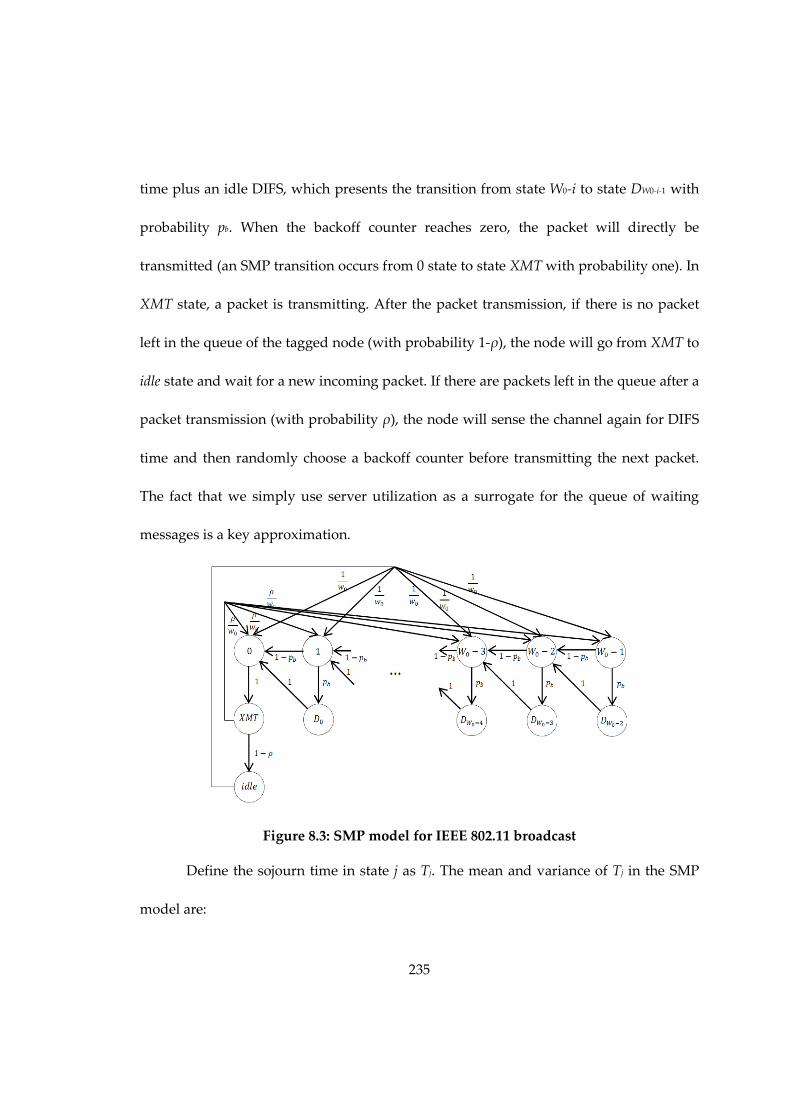
235

time plus an idle DIFS, which presents the transition from state W0-i to state DW0-i-1 with

probability pb. When the backoff counter reaches zero, the packet will directly be

transmitted (an SMP transition occurs from 0 state to state XMT with probability one). In

XMT state, a packet is transmitting. After the packet transmission, if there is no packet

left in the queue of the tagged node (with probability 1-ρ), the node will go from XMT to

idle state and wait for a new incoming packet. If there are packets left in the queue after a

packet transmission (with probability ρ), the node will sense the channel again for DIFS

time and then randomly choose a backoff counter before transmitting the next packet.

The fact that we simply use server utilization as a surrogate for the queue of waiting

messages is a key approximation.

Figure 8.3: SMP model for IEEE 802.11 broadcast


model are:

236

0

0

0 1 2

, 0,1,2,..., 1

, ,...,

[ ]

1

W

j j

j W

T j D D D

E T T j XMT

DIFS j idle

σ

τ

λ

−

= −

=

= = =

+ =

(8.2)

0

0

2

0 1 26

2

2

6

2

0, 0,1, 2,..., 1

1[ ] , ,...,

10[ ]

1[ ]

10

1/

W

d

j j

d

j W

Var PA j D D DR

Var T

Var PA j XMTR

j idle

θ

λ

−

= −

⋅ = ⋅

= =

⋅ = ⋅

=

(8.3)

where T=E[PA]/(Rd·106)+TH+DIFS+δ. The mean and variance of the packet transmission

time are E[PA]/(Rd·106) and Var[PA]/(Rd·106)2 respectively. Rd (Mbps) presents the data

rate. Hence, E[PA]/(Rd·106) is the time to transmit the packet. TH presents the packet

header transmission time including physical layer header time and MAC layer header

time. δ is the propagation delay.

For the SMP model in Fig. 8.3, the embedded DTMC is first solved for its steady-

state probabilities:

0

0 0

0

0

0 1 0

0 1 0 1 2

0 1

0 1

( ) , 0,1,2,..., 1

( 1) , ,...,

(1 )

W

b W W

i

W

W

W j v j W

W j p v j D D Dv

W v j XMT

W v j idleρ

−

− −

−

−

− = −

− − ==

=

− =

(8.4)

In the above equations,

0 1 2

0 0

2

(1 ) (5 2 )W

b b

vp W p Wρ

− =+ + − −

237

Taking into account the mean sojourn time in each state, the steady-state probabilities of

the semi-Markov process are given by:

i i

i

j j

j

v

v

τπ

τ=∑ (8.5)

Therefore, the steady-state probability that a node is in the XMT state is given

0

2

( ) 2 2(1 )(1 / )XMT

b b

T

p T W p T T DIFSπ

σ σ ρ λ=

+ + − + + − + (8.6)

Although the sojourn time in XMT state is T, the real packet transmission only

occupies a portion of this sojourn time, which is E[PA]/(Rd·106)+TH+δ=T-DIFS. Hence, the

probability that a node is transmitting in steady state is πXMT(T-DIFS)/T.

In Eq. (8.6), two unknown parameters are: ρ (the probability that there are

packets in the queue of the tagged vehicle) and pb (the probability that the channel is

detected busy in one time slot by the tagged vehicle). It is easy to see that pb of the

tagged vehicle depends on the transmitting state of other vehicles within the tagged

vehicle’s receiving range, and the transmitting probability of a vehicle can be described

by Eq. (8.6) (as a function of pb and ρ). Hence, pb of the tagged vehicle can be expressed

as a function of pb and ρ of other vehicles. Clealry, we have made the homogenity

assumption for all the vehicles. In addition, we know that ρ depends on the mean service

time to transmit a packet. Therefore, the service time is derived first in the next

subsection.

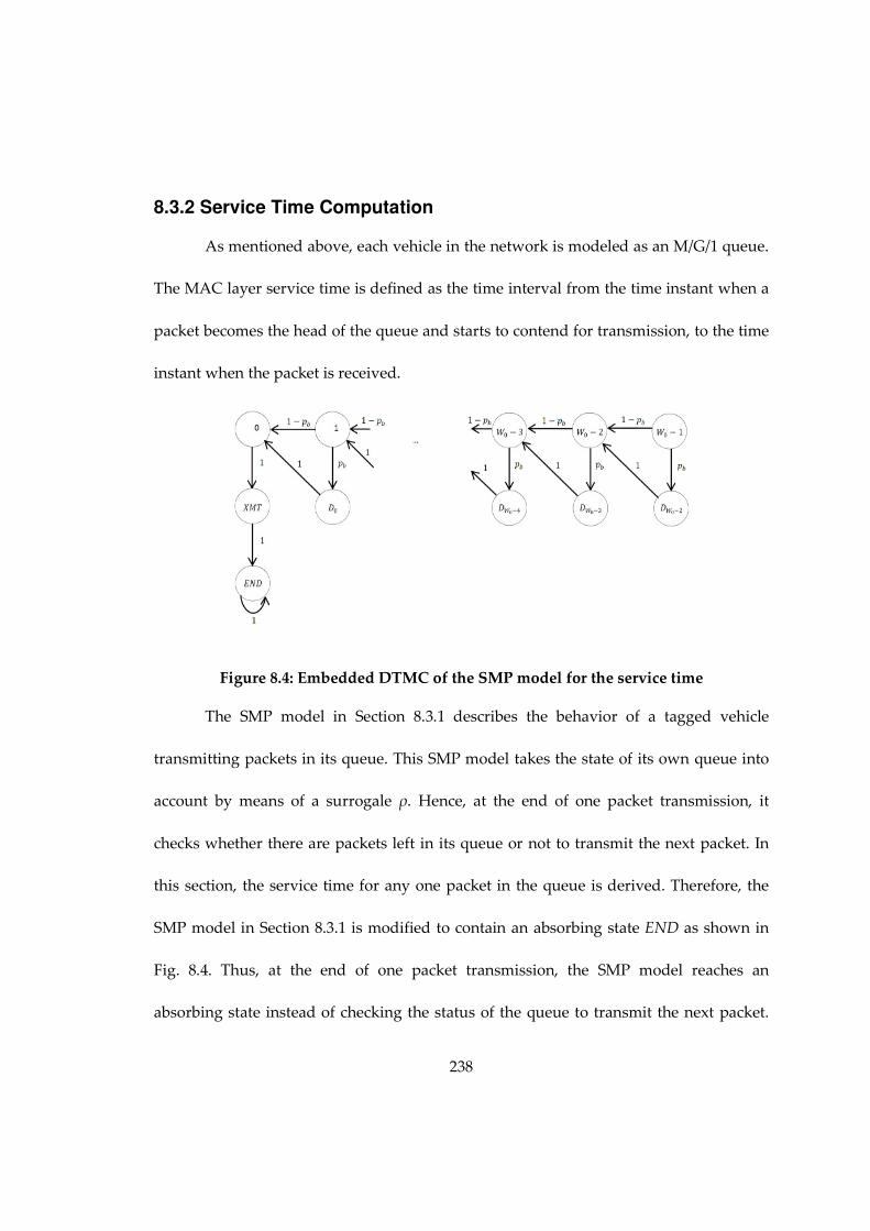
238


As mentioned above, each vehicle in the network is modeled as an M/G/1 queue.

The MAC layer service time is defined as the time interval from the time instant when a

packet becomes the head of the queue and starts to contend for transmission, to the time

instant when the packet is received.

Figure 8.4: Embedded DTMC of the SMP model for the service time

The SMP model in Section 8.3.1 describes the behavior of a tagged vehicle

transmitting packets in its queue. This SMP model takes the state of its own queue into

account by means of a surrogale ρ. Hence, at the end of one packet transmission, it

checks whether there are packets left in its queue or not to transmit the next packet. In

this section, the service time for any one packet in the queue is derived. Therefore, the

SMP model in Section 8.3.1 is modified to contain an absorbing state END as shown in

Fig. 8.4. Thus, at the end of one packet transmission, the SMP model reaches an

absorbing state instead of checking the status of the queue to transmit the next packet.

239

By proper choice of the initial probability vector, the time to reach the absorbing state

will be the service time for a packet transmission.

For a newly generated packet in the tagged vehicle, the vehicle will randomly

choose a backoff counter before the packet transmission. Therefore, the initial

probability that a packet starts its service from state i (i=0,1,…,W0-1) is 1/W0. Hence, the

initial probability vector is:

0

0

0

0 1 2 2

1 0,1,2,..., 1

0, , , ,..., ,

i

W

i WWq

i D D D D XMT−

= −

= =

(8.7)

Since the embedded DTMC contains an absorbing state (state END in Fig. 8.4),

taking advantage of the acyclic nature of the DTMC model in Fig. 8.4, the mean service

time for a packet transmission conditioned on starting from state i is derived from [12]:

0[ ] 0,1,..., 1

i bE S i i p T T for i Wσ= + ⋅ ⋅ + = − (8.8)

Therefore, the mean of the service time is given by

0( )( 1)

[ ] [ ]2

b

i i

i

p T WE S E S q T

σ + −= = +∑ (8.9)

8.3.3 Fixed-Point Iteration

In the previous section, the mean service time E[S] is shown to depend on two

unknown parameters ρ and pb. But ρ in turn depends on the mean service time as per

the M/G/1 queue equation ρ=λE[S]. As shown below, pb also depends on ρ. Because of

this cyclic dependence among the parameters, fixed-point iteration algorithm is utilized

to obtain the final converged solutions.

240

From the tagged vehicle’s point of view, pb is the probability that it senses

channel busy during one time slot in the backoff process. Since channel is detected busy

if there is at least one neighbor (i.e., a vehicle in the transmission range of the tagged

vehicle) transmitting in a backoff time slot of the tagged vehicle, we have

2 22

0

( )1 (1 ) 1

!cs cs XMT

i

L L Pi cs

b XMT

i

Lp P e e

i

βπ βπβπ∞− −

=

= − − = −∑ (8.10)

where PXMT is the probability that a neighbor is transmitting in a backoff time slot of the

tagged vehicle, to be derived later in this chapter.


capture the transmission of the neighbor is T-DIFS+2σ. One extra time slot σ is the one

just before transmission and another is the one just after transmission, which can capture

the starting time instant and ending time instant of the packet transmission. Therefore,

the probability that a neighbor’s transmission is detected in the first backoff time slot of

the tagged vehicle is πXMT(T-DIFS+2σ)/T.


the time duration that captures the transmission of the neighbor is 2σ [12]. Therefore, the

probability that a neighbor’s transmission is detected in non-first backoff time slot of the

tagged vehicle is πXMT×2σ/T.

Since the probability that a backoff time slot is the first backoff time slot is 1/W0

and non-first backoff time slot is (1-1/W0), the probability that a neighbor’s transmission

is detected by a backoff time slot of the tagged vehicle is given by

241

0 0

1 2 1 21

XMT XMT XMT

T DIFSP

W T W T

σ σπ π

− += + −

(8.11)

From the above analysis of the relationship between two parameters ρ and pb, we

notice that pb depends on ρ and pb itself. Hence, we denote pb=g(ρ,pb) and the reciprocal

of mean service time for M/G/1 queue to be µ=h(ρ,pb). The fixed-point iteration algorithm

is outlined below.

Step 1: Initialize ρ=1, which is the saturation condition;

Step 2: With ρ, solve pb using Eqs. (8.6)(8.10)(8.11);

Step 3: With ρ and pb, calculate service rate µ=1/E[S] using Eq. (8.9);

Step 4: If λ<µ, ρ=λ/µ; otherwise, ρ=1;

Step 5: If ρ converges, then stop the iteration. Otherwise, go to step 2 with the updated ρ.

By utilizing the fixed-point iteration, the parameters ρ, pb, πXMT as well as the mean and

the variance of the service time are determined, which are subsequently used for the

performance indices computation in the next section.

8.4 Performance Metrics

8.4.1 Mean Transmission Delay

The packet transmission delay is defined as the average delay a packet

experiences from the time at which the packet is generated until the time at which the

packet is successfully received by all neighbors of the node that generates the packet.

The transmission delay E[D] includes the queuing delay and medium service time (due

to backoff, packet transmission, and propagation delay, etc.).

242

The expected queuing delay is obtained from the Pollaczek-Khinchin mean value

formula of M/G/1 queue:

2[ ] ( [ ])[ ]

2(1 [ ])q

Var S E SE D

E S

λ

λ

+=

− (8.12)

The average packet transmission delay is then calculated as

[ ] [ ] [ ]q

E D E D E S= + (8.13)

8.4.2 Packet Delivery Probability

Packet Delivery Probability (PDP) (also is referred as Node Reception Probability in

Chapter 6-7) is defined as the probability that a node within the transmission range of

the sender successfully receives a packet from the tagged node (i.e., sender). There are

three factors affecting the performance of a packet reception: hidden terminal problems,

collisions due to concurrent packet transmissions, and interference as a result of the

fading channel.

φ

Figure 8.5: 2-D MANET model for performance analysis

243

The transmission scenario is shown pictorially in Fig. 8.5. Given a transmitting

node O placed at the origin, Q is one of the receivers within the transmission range (i.e.,

a circular coverage area having radius R) of node O. Q is placed on the x axis at a

distance r0 from O.

Let V: (r1cosΦ, r1sinΦ) be another node in the transmission range of O and Q. In

order to evaluate the impact of hidden terminals and concurrent transmissions on PDP,

two areas need to be considered. S1(r0)=D(Q, Lint)-D(O, Lcs) denotes the hidden terminal

area of node O, where D(s,l) represents the disk of radius l centered at s. Denote S2(Φ, r1,

r0)= D(V, Lcs)-D(O, Lcs) ∪ D(Q, Lint) as the area within the carrier sensing range of V that is

not in the carrier sensing range of O or interference range of Q.

a. Impact of Hidden Terminals

We observe that since the transmission time for a packet is T-DIFS=E[PA]/(Rd·106)+TH+δ,

the transmissions from hidden terminals collide with the tagged node’s transmission

only happens when hidden terminals start to transmit during the vulnerability period

2(T-DIFS)=2(E[PA]/(Rd·106)+TH+δ). Given the probability that a node starts to transmit

during the vulnerable period is πXMT·2(T-DIFS)/T [12], we have

1 0| ( )|1 0

0

0

1 0

| ( ) |2( )( ) 1

!

2( ) | ( ) |exp( )

i i

S r

H XMT

i

XMT

S rT DIFSP r e

T i

T DIFS S r

T

ββπ

β π

∞−

=

− = −

−= −

∑ (8.14)

where |S1(r0)| is the area of S1(r0). Derivation of |S1(r0)| is described next.

244

Figure 8.6: Illustration of S1 area calculation

As shown in Fig. 8.6, given distance r0 (r0<Lcs) between center O for circle D(O, Lcs) and

center Q for circle D(Q, Lint), intersection points of two circles denoted as I1 and I2, and X

the range on x axis projected by line I1O, we have equation:

2 2 2 2

int 0( )

csL X L r X− = − − (8.15)

Solve above equation, we obtain

2 2 2

0 int

02

csL r LX

r

+ −= (8.16)

Let ψ1, ψ2 be radian of I1O and I1Q, respectively. Then

2 2 2

0 int

1

0

2 2 2

0 int 0

2

int int 0

arccos arccos2

arccos arccos2

cs

cs cs

cs

L r LX

L L r

r X L r L

L L r

ψ

ψ

+ −= =

− + −= =

(8.17)

Denote S1’(r0) as the overlapping area of D(O, Lcs) and D(Q, Lint) , we have

2 2 2 2

1 0 1 int 2 0'( )

cs csS r L L r L Xψ ψ= + − − (8.18)

Therefore,

245

2

1 0 int 1 0| ( ) | | '( ) |S r L S rπ= − (8.19)

b. Impact of Concurrent Transmissions

In addition to collisions caused by the hidden terminals, transmissions from nodes

within the interference range of the tagged node in the meantime at which the tagged

node transmits may also cause collisions. When the tagged node transmits in a slot time,

concurrent collisions will take place if any node in the interference range of the tagged

node transmits in the slot.

Given that both O and Q sense the channel idle, V will transmit within the

duration of a slot with probability τ=π0. It should be noted that the slots of O and V are

not necessarily synchronized. Now, given that all nodes inside the union of two circles

center O, Q, radius R and Lint, respectively, are idle at the beginning of the slot, the

probability that a node V starts transmitting during the slot is the probability that node V

intends to transmit and all nodes in S2 are not in the transmitting state, which is

expressed as

2 1 0| ( , , )|2 1 0

2 1 0 0

1

0 2 1 0

( | ( , , ) |)'( , , ) (1 )

!

exp( | ( , , ) |)

i

S r ri

XMT

i

XMT

S r rP r r P e

i

P S r r

β ϕβ ϕϕ π

π β ϕ

∞−

=

= −

= −

∑ (8.20)

where |S2(Φ, r1, r0)| is the area of S2(Φ, r1, r0). Derivation of |S2(Φ, r1, r0)| is shown next.

246

φ

Figure 8.7: Illustration of S2 area calculation

Given coordinates of nodes P: (0,0), Q: (r0,0), and V: (r1cosΦ, r1sinΦ), the contour

functions of the transmission (or receiving) area of the nodes are: D(O, Lcs): x2+y2=Lcs2 ,

D(Q, Lint): (x-r0)2+y2=Lint2, D(V, Lcs): (x-r1cos Φ)2+(y-r1sin Φ)2=Lcs2.

Solve the above contour equations, we find the coordinates of all the intersection

points IPQ1, IPQ2, IPV1, IPV2, IQV1, and IQV2. Only three out of six intersection points determine

the shape of outmost contour. These intersection points can be selected through the

following criterion: if the given intersection point (x’, y’) is one of the outmost

intersection points, the following inequities must hold

2 2 2

2 2 2

0 int

2 2 2

1 1

' '

( ' ) '

( ' cos ) ( ' sin )

cs

cs

x y L

x r y L

x r y r Lϕ ϕ

+ ≥

− + ≥

− + − ≥

(8.21)

It is easy to prove that the criterion is both sufficient and necessary.

By knowing the outmost intersection points and corresponding outmost curves,

we are able to calculate the area surrounded by the outmost contour. Two neighboring

outmost intersection points determine one outmost curve. Outmost curves all together

247

form the outmost contour. In Fig. 8.7, the outmost contour consists of the following

curves:

Given the three outmost intersection points I1 with coordinate (x1, y1), I2 with

coordinate (x2, y2), and I3 with coordinate (x3, y3), whose radian coordinates are (ri1, θ1),

(ri2, θ2), and (ri3, θ3), respectively, where ri1= ri3=Lcs; ri2= (xi22+yi22)1/2; θ1=arctg(yi1/xi1),

θ2=arctg(yi2/xi2), θ3=arctg(yi3/xi3).

Outmost curves connected by I1, I2, and I3 divide the total area into two sections:

section 1 (I1I2) center V and section 2 (I2I3) center Q, as shown in Fig. 8.7. Areas of the

two sections are denoted as A1 and A2, respectively. Given O at the origin, radian of

section 1 ranges from θ2 to θ1; radian of section 2 ranges from θ3 to θ2; and radian of VO

is Φ.

Given that P is a point on the outmost curve of section 1 and the radian of PO is

θ, the area of section 1 is:

1

2

1

2

2

1

2 2 2 2

1 1

2 2

2 212 21 1 2

1 1

2 1

1

2

1| |

2

1( cos( ) sin ( ))

2

sin( ) ( ) sin ( )( )( ) sin 2( )

[ ]2 2 4 2

sin( )arcsin( )

2

cs

cs

cs

cs

cs

A PO d

r L r d

L

rL rr r

rL

L

θ

θ

θ

θ

θ

θ ϕ θ ϕ θ

θ ϕ θ ϕθ θ θ ϕ θ ϕ

θ ϕθ

θ

=

= − + − −

− − −− − − −

= + + −

−

−

∫

∫

(8.22)

Given that U is a point on the outmost curve of section 2 and the radian of UO is θ, the

area of section 2 is:

248

2

3

2

3

2

2

2 2 2 2

0 int 0

2 2int 2 0int2 2

202 2int 0 2 3 int

0 0

3

1| |

2

1( cos sin )

2

sinsin ( ) sin arcsin( )

( )( ) sin(2 )[ ]

2 2 4 2 2

A UO d

r L r d

L rL

rL r Lr r

θ

θ

θ

θ

θ

θ θ θ

θθ θ

θθ θ θ θ

θ

=

= + −

−− −

= + + − −

∫

∫ (8.23)

Then, the extended coverage area S2(Φ, r1, r0), as shown in Fig. 8.7, can be calculated as

the sum of A1 and A2 excluding the area of D(O, R) and node O’s hidden terminal area in

A1 and A2, which is expressed as:

2

2 1 0 1 2 1 3 1 0

1( , , ) ( ) | ( ) |

2cs

S r r A A L S rϕ θ θ= + − − − (8.24)

Therefore, the average number of nodes that start transmission during the slot

that collides with the transmission from O within the circle with center Q radius Lint is

int2

2 00 0

'( , , )L

Tn rP r r drdπ

β ϕ ϕ= ∫ ∫ (8.25)

Therefore, given Poisson node distribution, the probability that no node within

the circle center Q radius Lint start transmission during the slot that collides with the


0

0

( )( ) exp( ) exp( )

0!

TTcon T

nP r n n= − = − (8.26)

c. Impact of Channel Fading and Path Loss

VANETs present scenarios with unfavorable characteristics to develop wireless

communications, i.e., multiple reflecting objects able to degrade the strength and quality

of the received signal. Additionally, fading effects resulting from the mobility of the

249

surrounding objects and/or the sender and receivers themselves have to be taken into

account. Therefore, similar to Section 7.3.1 in Chapter 7, we incorporate the channel

fading’s effect and the probability of successfully receiving a message at a distance r0

considering channel fading with path loss effects is given by:

( )( )0 /

1

00

1 e( )

mr R

m mz

F

mP r z dz

m

γ

− −= −Γ ∫ (8.27)

Taking hidden terminals, possible packet collisions, and channel fading with path loss

into account, and assuming these three events are independent, the probability that the

node Q receives the broadcast message from the tagged node O is:

0 0 0 0( ) ( ) ( ) ( )

s H F conP r P r P r P r= (8.28)

8.4.3 Packet Reception Ratio

Packet Reception Ratio (PRR) is defined as the percentage of nodes that

successfully receive a packet from the tagged node given that all receivers are within the

transmission range of the sender at the moment that the packet is sent out [3]. From the

above definition, PRR can be interpreted as the percentage of the mobile nodes in the

tagged node’s transmission range that receive the broadcast message successfully.

We approach PRR evaluation in two steps. First, compute the probability that the

individual node Q successfully receives the broadcast packet from the sender O. Then,

PRR is derived through integration of the probabilities over the transmission range of O.

Assuming the distribution of nodes along a 2-D area follows Poisson process, the

average number of nodes within an incremental area dA should be βdA [110]. Given the

250

reception probability of each node in Eq. (8.28), the average number of nodes within dA

that successfully receive the broadcast message from the tagged node is Ps(r)βdA. For a

circular coverage area having radius R from node O, PRR over a coverage area with

radius d (d≤R) found by integrating the probabilities that nodes with distance r to the

source node O within an incremental area dA successfully receive the broadcast message

from O. Hence,

2

2 20 0 0

1 2( ) ( ) ( )

d d

s sPRR d P r rdrd P r rdrd d

π

ϕπ

= =∫ ∫ ∫ (8.29)


Table 8.1: DSRC communication parameter

Parameters Values Parameters Values Modulation BPSK, QPSK, 16-QAM, 64-QAM Slot time, σ 16 µs

Coding Rates 1/2, 2/3, 3/4 SIFS 32 µs

OFDM Symbol

Duration 8 µs Propagation delay, δ 1 µs

Signal Bandwidth 10 MHz Preamble Length 40 µs

Channel Data rate 6, 9, 12, 36, 54 Mbps PLCP Header Length 8 µs

DIFS 64 µs CWMin 15~1024

In this section, we apply the proposed model to a typical VANET environment:

vehicular ad hoc communication system in battlefield. Each node is equipped with IEEE

802.11 based wireless ad hoc network capability with communication parameters as

listed in Table 8.1. Communication range (transmission/carrier sensing) is R=500 m. Each

node generates broadcast messages with rate λ and the average message length

E[PA]=200~400 bytes. Two dimensional numerical integrations in MATLAB (double

integral over rectangle) are used to compute overlapping areas and the impact of

251

Nakagami fading needed for derivation of PRRs. In order to cross-validate the proposed

analytic model, we extend 1-D event-driven simulation program developed for research

in [36] to 2-D simulation with Nakagami fading and path loss using both NS2 and

MATLAB. The communication nodes are Poisson distributed with density β (nodes/m2)

on a 2-D area with radius of 3000 m. The free space propagation model is adopted (γ=2).

Most of assumptions made in the analytic solution are relaxed in the simulation. In the

NS2 program, the communication nodes are connected through setting up transmission

powers and receiving thresholds so that the communication ranges are random

variables. With distributed asynchronous time scale and limited communication ranges,

asynchronous time channel access and the hidden terminal problem are naturally

reflected in the simulation process. In addition, different from the decomposition

method used in the analytic model, the simulation process simulates the overall system

behavior.

Figure 8.8: PRR with W0=15

252

Figure 8.9: Mean transmission delay with W0=15

Figure 8.10: Impact of Nakagami fading on PRR of DSRC broadcast with

network parameters W0=15, λ=10 packets/s, Rd=24Mbps

253

Figure 8.11: PRR and PDP of DSRC broadcast with network parameters W0=15,

Rd=24Mbps, β=100/(πR2)

Figure 8.12: PDP with network parameters λ=10 packets/s, W0=15, Rd=24Mbps,

β=100/(πR2)

254

Figure 8.13: Impact of Communication range on PRR of DSRC broadcast with

network parameters W0=15, λ=10 packets/s, Rd=24Mbps

Fig. 8.8 and Fig. 8.9 depict the packet reception ratios (PRRs) and packet

transmission delay, respectively, over the average number of nodes in the transmission

range of a transmitting (or tagged) node. As shown in Fig. 8.8 and Fig. 8.9, analytical

results (lines) practically coincide with the simulation results (symbols). The relative

errors between analytical results and simulation results are 0.84% for PRRs, and 3.45%

for packet transmission delays. We also observe that PRRs get lower with the density of

nodes in the network because more nodes introduce more data traffic on the ad hoc

broadcast network. Fig. 8.8 also shows that increasing packet generation rate λ (from 2

packets/second to 10 packets/second) degrades PRRs since more collisions and

transmissions of hidden terminals are introduced as the packet generation rate λ goes

up. This degradation cannot be compensated by lifting transmission data rate (from 12

255

Mbps to 24 Mbps). From Fig. 8.8, we can see a significant difference between PRRs with

Nakagami fading (m=3) and PRRs without any fading, which indicates that, in addition to

hidden terminal problem, channel fading is another major factor for the degradation of

reliability. From Fig. 8.9, we observe that channel fading does not affect the packet

transmission delay.

Fig. 8.10 shows how Nakagami fading with different m values affect PRRs of the

MANET broadcast communication. As stated earlier, fading degrades PRRs

significantly. PRRs with m=3 are bigger than PRRs with m=1 (Rayleigh distribution),

which means bigger fading parameters bring smaller fading to the communications.

Fig. 8.11 demonstrates how packet reception ratios (PRRs) and packet delivery

probability (PDPs) of a node change with the receivers’ distances to the sender. Both

PRRs and PDPs are reduced with the receiver’s distance to the sender, and are degraded

with much higher rate as the receiver’s distance to the sender is longer than 300 m. The

observation is due to the fact that the longer the receiver’s distance to the sender, the

more likely the receiver is affected by hidden terminals problem and channel fading.

This observation alleviates the difficulty of selecting network parameters to meet the

strict reliability requirements in some applications such as VANET safety message

broadcast where high PRR is required for the receiving nodes that are closer to the

transmitting node.

256

Fig. 8.12 shows how PDPs are affected by respective factors listed as hidden

terminal problem, concurrent collisions, and channel fading. Given the same network

parameters, separate PDP curves ignoring individual factors are compared with PDPs

taking all factors into account. It is observed that the curve without accounting for

Nakagami fading has the biggest difference from the curve taking all factors into account

among the other two curves, and the curve without accounting for concurrent collisions

has the smallest difference from the curve taking all factors into account among the

other two curves. This observation reveals that fading channel and hidden terminals

problem are major factors to degrade the broadcast reliability, while concurrent

collisions affect the reliability slightly.

Fig. 8.13 depicts the impact of communication ranges on the reliability with

certain network setting. When carrier sensing range increases from 500 m to 1000 m

(means w/o hidden terminals), PRRs increase accordingly because the bigger the carrier

sensing range, the less the number of hidden terminals. It is interesting to see that the

impact of fading is more significant than the impact of hidden terminals. If the

interference range increases (from 500 m to 600 m), PRRs are getting worse even though

carrier sensing range is extended (from 500 m to 800 m).

8.6 Conclusions

In this chapter, we propose an analytical model to evaluate the performance of

IEEE 802.11 based broadcast two-dimensional VANETs. A semi-Markov process model

257

interacts with M/G/1 queuing model to characterize the behavior of communicating

nodes under IEEE 802.11 broadcast. The derived PRR expressions take into account the

impact of Nakagami fading channel with path loss, hidden terminals problem, concurrent

transmissions, unsaturated message arrivals and varied communication ranges of IEEE

802.11 MAC, and DCF backoff process. As an example, the analytical model is applied to

a vehicular ad hoc system for the broadcast of safety messages. PRR derivation using

point-to-point integration facilitates the accurate impact analysis of fading channel.

Numerical results prove the effectiveness and correctness of the proposed model, and

reveal the characteristics of 2-D broadcast VANETs, which can be beneficial to the

design of such systems. From the numerical results and discussions, some very

important observations of such networks are described. Our future research will focus

on building more specific models to fit various road conditions such as intersections,

streets of cities, etc., and extend the proposed 2-D model to the models with more

general node distributions and more general packet arrivals.

258

9. Summary

In this chapter, we summarize the work in this dissertation. The main theme of

this dissertation is to develop comprehensive and high fidelity analytic models for the

effective performance and reliability analysis of various V2V DSRC safety

communication scenarios. A major hurdle in the development of VANET for safety-

critical services in the DSRC system is the lack of established models and metrics which

can be utilized to determine the effectiveness of VANET design mechanisms for

predictable QoS and allows one to evaluate the tradeoff between network parameters.

Simulation methods usually consume long time to collect sufficient data for accurate

system performance analysis. Real world testbeds can capture more practical network

dynamics but are limited by extremely high equipment cost. In this dissertation, we

have proposed accurate and efficient analytic models to assess the effectiveness of

message dissemination schemes for safety applications. Important MAC and application

level performance and reliability metrics are derived and evaluated. The major point is

that analytic models that reflect important details of the protocol and user behavior can

be developed and solved efficiently thus avoiding costly simulations. Based on the

numerical results, we also analyze the tradeoff of network parameters and provide

insights to tune the network parameters to meet the application requirements.

In Chapter 3, we presented a general analytic model to evaluate the performance

of safety message broadcasting, which is suitable for event-driven safety messages

259

(ESMs) assuming Poisson arrivals and infinite MAC-layer queue. To produce a tractable

analytic model, we utilize model decomposition and fixed-point iteration to obtain

converged solutions. Important MAC-level performance and reliability metrics are

subsequently derived. Chapter 4 describes a more accurate analytic model compared to

Chapter 3 to capture the basic safety messages (BSMs) broadcasting, where associated

features such as periodic message generation, out-dated message replacement and no

queuing in MAC-layer are incorporated. Such a model for BSMs is compared with the

model presented in Chapter 3 for ESMs. The results prove that the simplified analytic

model for ESMs can be used to approximately evaluate the BSMs transmission. Besides

MAC-level metrics, application-level metrics are also derived in Chapter 4. Simulations

in Matlab are conducted for the comparison purpose in both Chapter 3 and 4.

Since different types of messages (including BSMs and ESMs with different

priorities) maybe transmitted in a single channel, in Chapter 5, multiple types of services

transmission over a single channel (e.g., control channel) is evaluated based on the

extension of the analytic model developed in Chapter 3. The EDCA mechanism specified

in the IEEE 802.11p protocol is shown to be ineffective to guarantee priorities for

different services. Important conclusions are also drawn to tune network parameters in

order to improve the performance and reliability for high priority services.

At the early stage of DSRC technology deployment, a radio device can switch

between channels to support concurrent applications on different channels. Therefore, in

260

Chapter 6, we consider IEEE 1609.4 multi-channel operation’s impact to evaluate the

performance and reliability of the BSMs transmission on the control channel (CCH). The

impact of various factors such as concurrent transmission, hidden terminals problem,

channel fading with path loss and channel switching mechanism are evaluated.

Simulations are developed in NS2 to validate the accuracy and efficiency of the

proposed analytic model.

Channel 172 may be reserved for highly critical safety applications with no time

division, and hence ESMs are most likely to be transmitted in Channel 172. Since some

event-driven safety applications (e.g., post-crash notification, road hazard warning) may

require longer transmission distance than the one-hop communication range, multi-hop

dissemination of ESMs is necessary. Therefore, Chapter 7 introduces an accurate analytic

model to evaluate multi-hop propagation of ESMs. Extensive Matlab simulations are

performed to cross-validate the analytic model. Important conclusions are drawn to

provide deeper understandings of the performance and reliability of the ESMs

transmission behavior.

Besides 1-D traffic scenario presented in Chapter 3-7, we first introduce an

analytic model for the performance and reliability evaluation of 2-D traffic at open field

to capture more realistic message transmission behaviors. Simulations in NS2 are carried

out and the numerical results are compared with the analytic-numerical results under a

large range of network parameter settings.

261

In future, vehicle mobility may be taken into account to characterize the dynamic

behavior in vehicular safety communications. Even though vehicle mobility has been

proven that high mobility of vehicles has very minor impact on the performance of the

direct message broadcasting with high data rate, it may have great impact on

application level performance metrics. In addition, more realistic two-dimensional traffic

scenarios such as intersections, parallel lanes and square grid for downtown area will be

considered.

For event-driven safety messages that are highly critical to safety on the road, it

is essential to ensure their successfully transmission. Therefore, the safety message can

be broadcasted multiple times over the communication range to increase the receptions

probability, which is referred as one-hop multi-cycle broadcast. However, due to the

increase number of packets transmitted resulting from rebroadcast of the same message,

the packets will suffer from more collisions. Therefore, the evaluation of multi-cycle

broadcast of safety messages is necessary to ensure the effective of multi-cycle schemes.

The analytic model will also be extended to incorporate different packet arrival

processes such as Markov modulated Poisson process (MMPP), Markovian arrival

process (MAP) etc. to capture more general safety message generations. For event-

driven safety messages that generated occasionally for a vehicle, it is possible that the

over different time periods, safety messages are generated with different arrival rates.

For example, the emergency events may occur quite less frequently over an area in

262

which vehicle density is low or road condition is very good, while occur more frequently

over another area in which vehicle density is high or road condition is bad. For such

scenario, MMPP can be used to capture the packets arrivals instead of assuming Poisson

arrival for event-driven safety messages.

263

Bibliography

[1] ASTM E2213-03, “Standard Specification for Telecommunications and Information

Exchange Between Roadside and Vehicle Systems 5GHz Band Dedicated Short

Range Communications (DSRC) Medium Access Control (MAC) and Physical Layer

(PHY) Specifications”, ASTM Intl. Jul, 2003.

[2] J. Yin, T. Elbatt, et al., “Performance evaluation of safety applications over DSRC

vehicular ad hoc networks”, ACM VANET, pp. 1-9, 2004.

[3] M. T. Moreno, D. Jiang, and H. Hartenstein, “Broadcast reception rates and effects of

priority access in 802.11-based vehicular ad-hoc networks”, ACM VANET, pp. 10-18,

2004.

[4] Q. Xu, T. Mak, J. Ko, and R. Sengupta, “Vehicle-to-vehicle safety messaging in

DSRC”, ACM VANET, pp. 19-28, 2004.

[5] F. Bai and H. Krishnan, “Reliability analysis of DSRC wireless communication for

vehicle safety applications”, IEEE Intelligent Transportation Systems Conference,

ITSC’06., pp. 355–362, Sept. 2006.

[6] X. Ma, X. Chen, and H. H. Refai, “Unsaturated performance of IEEE 802.11 broadcast

service in vehicle-to-vehicle networks”, IEEE VTC, pp. 1957-1961, 2007.

[7] X. Chen, H. H. Refai, and X. Ma, “A Quantitative Approach to evaluation DSRC

Highway Inter-vehicle Safety Communication”, IEEE GLOBECOM, pp. 151-155,

2007.

[8] X. Ma, X. Chen, and H. H. Refai, “Performance and reliability of DSRC vehicular

safety communication: a formal analysis”, EURASIP J. on Wireless Comm. and

Networking, pp. 1-13, 2009.

[9] K. S. Trivedi, Probability and Statistics with Reliability, Queuing and Computer Science

Applications, Second Edition, John Wiley, 2002.

[10] L. Tomek and K.S. Trivedi, “Fixed-Point Iteration in Availability Modeling”,

Informatik-Fachberichte, Vol. 283, M. DalCin (ed.), pp. 229-240, Springer-Verlag, Berlin,

1991.

[11] IEEE 802.11 Working group, “Part 11: wireless LAN medium access control

(MAC) and physical layer (PHY) specifications”, ANSI/IEEE Std. 802.11, Sep. 1999.

264

[12] X. Yin, X. Ma and K. S. Trivedi, “Performance Evaluation for DSRC Vehicular

Safety Communication: A Semi-Markov Process Approach”, International Conference

on Communication Theory, Reliability, and Quality of Service, 2011.

[13] P. D. Welch, “On a Generalized M/G/l Queueing Process in which the First

Customer of Each Busy Period Receives Exceptional Service”, Operations Research,

Vol, 12, No, 5, pp. 736-752, 1964.

[14] V. Mainkar and K. S. Trivedi, “Sufficient conditions for existence of a fixed point

in stochastic reward net-based iterative models”, IEEE Transactions. on Software

Engineering, 1996.

[15] G. Haring, R. Marie, R. Puigjaner, K.S. Trivedi, “Loss formulae and their

optimization for cellular networks”, IEEE Transactions on Vehicular Technology, 50 (3)

pp. 664-673, 2001.

[16] G. Ciardo and K. S. Trivedi, “A Decomposition Approach for Stochastic Reward

Net Models”, Performance Evaluation, 18(1), pp. 37-59, 1993.

[17] J. Medhi, Stochastic Processes, Wiley Eastern, New Delhi, 1994.

[18] J. M. Ortega and W. C. Rheinboldt, Iterative Solution of Nonlinear Equations in

Several Variables, Academic Press, 1970.

[19] P. M. Fitzpatrick, Advanced Calculus, 2nd edition, Thomson, Brooks/Cole, 2006.

[20] R. L. Burden, J. D. Faires, Numerical Analysis, 7th edition, Brooks/Cole, 2000.

[21] S. C. Malik, S. Arora, Mathematical Analysis, 3rd edition, New Age Science, 2009.

[22] E. Cinlar, Introduction to Stochastic Processes, Prentice-Hall, Englewood Cliffs,

New Jersey, 1975.

[23] X. Ma and X. Chen, “Performance analysis of IEEE 802.11 broadcast scheme in ad

hoc wireless LANs”, IEEE Transactions on Vehicular Technology, 57(6): 3757-3768, Nov.

2008.

[24] F. Ye, R. Yim, S. Roy, and J. Zhang, “Efficiency and reliability of one-hop

broadcasting in vehicular ad hoc networks”, IEEE Journal of Selected Areas in

Communications, 29(1): 151-160, Jan. 2011.

265

[25] Md. I. Hassan, H. L. Vu, T. Sakurai, “Performance analysis of the IEEE 802.11

MAC protocol for DSRC with and without retransmissions”, IEEE Int. Symposium on

a World of Wireless Mobile and Multimedia Networks, 2010.

[26] C. Campolo, A. Vinel, A. Molinaro, Y. Koucheryavy, “Modeling Broadcasting in

IEEE 802.11p/WAVE Vehicular Networks”, IEEE Communications Letters, vol.15, no.2,

pp.199-201, February 2011.

[27] G. Bianchi, “Performance analysis of the IEEE 802.11 distributed coordination

function”, IEEE Journal on Selected Areas in Communications, vol.18, no.3, pp.535-547,

Mar 2000.

[28] J. W. Robinson and T. S. Randhawa, “Saturation throughput analysis of IEEE

802.11e enhanced distributed coordination function”, IEEE Journal on Selected Areas in

Communications, vol. 22, no. 5, pp. 917–928, Jun. 2004.

[29] R. Battiti and B. Li, “Supporting service differentiation with enhancements of the

IEEE 802.11 MAC protocol: models and analysis”, University of Trento, Italy, Tech.

Rep. DIT-03-024, May 2003.

[30] D. Malone, K. Duffy, D. Leith, “Modeling the 802.11 Distributed Coordination

Function in Nonsaturated Heterogeneous Conditions”, IEEE/ACM Transactions on

Networking, vol.15, no.1, pp.159-172, Feb. 2007.

[31] J.R. Gallardo, D. Makrakis, and H.T. Mouftah, “Mathematical Analysis of

EDCA's Performance on the Control Channel of an IEEE 802.11 WAVE Vehicular

Network”, EURASIP Journal on Wireless Communications and Networking, 2010.

[32] G. Badawy, J. Misic, T. Todd, and D. Zhao, “Performance Modeling of Safety

Message Delivery in Vehicular Ad Hoc Networks”, IEEE WiMob, 2010.

[33] J. R. Gallardo, D. Makrakis, and H. T. Mouftah, “Performance analysis of the

EDCA medium access mechanism over the control channel of an IEEE 802.11p

WAVE vehicular network”, IEEE International Conference on Communications (ICC),

pp. 1-6, 2009.

[34] N. Wisitpongphan, B. Fan, P. Mudalige, V. Sadekar, O. Tonguz, “Routing in

sparse vehicular ad hoc wireless networks”, IEEE Journal on Selected Areas in

Communications, 25(8): 1538-1556, 2007.

266

[35] H. Zhu, L. Fu, G. Xue, Y. Zhu, M. Li, L. Ni, “Impact on traffic influxes:

understanding exponential inter-contact time in VANETs”, IEEE INFOCOM’10,

2010.

[36] X. Ma, J. Zhang, T. Wu, “Reconsider Broadcast Packet Reception Rates in One-

Dimensional MANETs”. IEEE GLOBECOM, 2010: 1-6.

[37] I. Tinnirello, G. Bianchi, “Rethinking the IEEE 802.11e EDCA performance

modeling methodology”. IEEE/ACM Transactions on Networking (TON), 18(2):540-553,

2010.

[38] J. Y. Lee, H. S. Lee, “A performance analysis model for IEEE 802.11e EDCA

under saturation condition”. IEEE Transactions on Communications (TCOM) 57(1):56-

63, 2009.

[39] F. Bai and B. Krishnamachari, “Spatio-temporal Variations of Vehicle Traffic in

VANETs: Facts and Implications”. In ACM VANET, 2009.

[40] M. T. Moreno, S. Corroy, H. Hartenstein, “IEEE 802.11-based one-hop broadcast

communications: understanding transmission success and failure under different

radio propagation environments” ACM International Workshop on Modeling Analysis

and Simulation of Wireless and Mobile Systems (MSWiM’06), pp. 68-77, Spain, 2004.

[41] X. Ma and X. Chen, “Delay and Broadcast Reception Rates of Highway Safety

Applications in Vehicular Ad Hoc Networks”, IEEE INFOCOM2007 Workshop on

Mobile Networks for Vehicular Environments, pp. 85-90, 2007.

[42] M. V. Eenennaam, W. K. Wolterink, G. Karagiannis, and G. Heijenk, “Exploring

the Solution Space of Beaconing in VANETs”, In: First IEEE Vehicular Networking

Conference, VNC2009, 28-30 Oct 2009, Tokyo, Japan.

[43] X. Chen, H. H. Refai, X. Ma, “Saturation Performance of IEEE 802.11 Broadcast

Scheme in Ad Hoc Wireless LANs”, IEEE VTC Fall 2007: 1897-1901.

[44] IEEE Standard for Information Technology-Telecommunications and

Information Exchange between Systems-Local and Metropolitan Area Networks-

Specific Requirements; Part 11: Wireless LAN Medium Access Control (MAC) and

Physical Layer (PHY) Specifications; Amendment 6: Wireless Access in Vehicular

Environments, IEEE Std. 802.11p, Jul. 2010.

[45] J. B. Kenney, “Dedicated short range communications (DSRC) standards in the

United States”, Proceedings of the IEEE, vol. 99, no. 7, pp. 1162-1182, 2011.

267

[46] “Dedicated Short Range Communications (DSRC) Message Set Dictionary”, SAE

Std. J2735, SAE Int., DSRC Committee, Nov. 2009.

[47] T. A. ElBatt, S. K. Goel, G. Holland, H. Krishnan, J. S. Parikh, “Cooperative

collision warning using dedicated short range wireless communications,” Proceeding

of ACM VANET workshop, 2006.

[48] S. Yousefi, M. Fathy and A. Benslimane, “Performance of beacon safety message

dissemination in Vehicular Ad hoc NETworks (VANETs),” Journal of Zhejiang

University SCIENCE A, 2007.

[49] M. Torrent-Moreno “Inter-Vehicle Communications: Achieving Safety in a

Distributed Wireless Environment: Challenges, Systems and Protocols”, PhD-

dissertation, Karlsruhe, 2007.

[50] A. Vinel, V. Vishnevsky, Y. Koucheryavy, “A simple analytical model for the

periodic broadcasting in vehicular ad-hoc networks”, Proc. 4th BWA Workshop, co-

located with IEEE GLOBECOM, 2008.

[51] S. Bastani, B. Landfeldt and L. Libman, “On the Reliability of Safety Message

Broadcast in Urban Vehicular Ad hoc Networks”, Proc. ACM int. conf. on Modeling,

Analysis and Simulation of Wireless and Mobile Systems, 2011.

[52] X. Yin, X. Ma, and K. S. Trivedi, “An Interacting Stochastic Models Approach for

the Performance Evaluation of DSRC Vehicular Safety Communication”, IEEE

Transactions on Computers, vol. 62, no. 7, 2013.

[53] F. Bai, H. Krishnan, V. Sadekar, G. Holland, T. ElBatt, “Towards characterizing

and classifying communication-based automotive applications from a wireless

networking perspective”, IEEE Workshop on Autonet, 2006.

[54] N. An, T. Gaugel, and H. Hartenstein, “VANET: is 95% probability of packet

reception safe?” IEEE 11th International Conference on ITS Telecommunications, 2011.

[55] H. Lu, and C. Poellabauer, “Analysis of application-specific broadcast reliability

for vehicle safety communications”, ACM VANET’11.

[56] K. Matthes, Zur Theorie der Bedienungsprozesse, in: Trans. of the 3rd Prague

Conf. on Information Theory, Stat. Dec. Fns. and Random Processes, 1962, pp. 513–

528.

268

[57] P. Glynn, “A GSMP formalism for discrete event systems”, Proc. of the IEEE, 77,

(1989).

[58] ETSI TC ITS, “ITS; Vehicular Communications; Basic Set of Applications;

Definitions”, Tech. Rep. TR 102 638, 2009.

[59] A. Buchenscheit, F. Schaub, F. Kargl, M. Weber, “A VANET-based emergency

vehicle warning system”, IEEE Vehicular Networking Conference (VNC), pp.1-8, 28-30

Oct. 2009.

[60] R. Chen, D. Ma, and A. Regan, “TARI: Meeting Delay Requirements in VANETs

with Efficient Authentication and Revocation”, IEEE International Conference on

Wireless Access in Vehicular Environment, 2009.

[61] Q. Chen, D. Jiang, L. Delgrossi, “IEEE 1609.4 DSRC Multi-Channel Operations

and Its Implications on Vehicle Safety Communications” VNC 2009.

[62] A. Lyakhov, V. Vishnevsky, and P. Poupyrev, “Analytical Study of Broadcasting

in 802.11 Ad Hoc Networks”, Proc. 2nd International Conference on e-Business and

Telecommunication Networks (ICETE 2005), October 3-7, 2005, Reading, U.K. Vol. II,

pp.86-91

[63] “IEEE Trial-Use Standard for Wireless Access in Vehicular Environments

(WAVE) – Multi-Channel Operation,” IEEE 1609.4-2006.

[64] K. Hong, J. B. Kennedy, V. Rai and K. P. Laberteaux, “Evaluation of Multi-

Channel Schemes for Vehicular Safety Communications”, in Proc. of IEEE VTC-

Spring, Taipei, pp. 1-5, 2010.

[65] J. Misic, G. Badawy and V. Misic, “Performance Characterization for IEEE

802.11p Network with Single Channel Devices”, IEEE Transactions on Vehicular

Technology, 68(4), pp. 1775-1789, 2011.

[66] A. J. Ghandour, M. D. Felice, L. Bononi, H. Artail, “Modeling and simulation of

WAVE 1609.4-based multi-channel vehicular ad hoc networks”, Proceedings of the 5th

International ICST Conference on Simulation Tools and Techniques, pp. 148-156, 2012

[67] Y. Du, L. Zhang, Y. Feng, Z. Ren and Z. Wang, “Performance Analysis and

Enhancement of IEEE 802.11p/1609 Protocol Family in Dense Vehicular

Environments”, In Proc. of 13th International IEEE Conference on Intelligent

Transportation Systems, ITSC 2010, 19-22 Sep 2010.

269

[68] X. Yin, X. Ma and K. S. Trivedi, “MAC and Application Level Performance

Evaluation of Beacon Message Dissemination in DSRC Safety Communication”,

submitted to Performance Evaluation, 2012.

[69] IEEE Trial-Use Standard for Wireless Access in Vehicular Environments

(WAVE)—Multi-Channel Operation, IEEE Std. 1609.4-2007, 2007.


(WAVE)—Networking Services, IEEE Std. 1609.3-2007, 2007.


(WAVE)—Security Services for Applications and Management Messages, IEEE Std.

1609.2-2007, 2007.

[72] X. Ma, X. Yin and K. S. Trivedi, “Performance Evaluation of Two-Dimensional

Broadcast Ad Hoc Network”, submitted to IEEE Transaction on Computers, 2012.

[73] X. Ma, J. Zhang, X. Yin, and K. S. Trivedi, “Design and analysis of a robust

broadcast scheme for vanet safety-related services,” IEEE Transactions on Vehicular

Technology, vol. 61, no. 1, pp. 46–61, Jan 2012.

[74] A. Vinel, “3GPP LTE Versus IEEE 802.11p/WAVE: Which Technology is Able to

Support Cooperative Vehicular Safety Applications?”, IEEE Wireless Communication

Letters, Vol. 1, No. 2, April 2012.

[75] S. Bastani, B. Landfeldt, and L. Libman, “A traffic density model for radio

overlapping in urban vehicular ad hoc networks”, IEEE Conference on Local Computer

Networks (LCN), Bonn, Germany, Oct. 2011.

[76] S. Bastani, B. Landfeldt, and L. Libman, “On the reliability of safety message

broadcast in urban vehicular ad hoc networks”, ACM MSWiM’11, Miami Beach,

2011.

[77] A. Zanella, G. Pierobon, and S. Merlin, “On the limiting performance of

broadcast algorithms over unidimensional ad hoc radio networks”, WPMC’ 04, Italy,

Sep. 2004.

[78] S. Ni, Y. Seng, Y. Chen and J. Sheu, “The broadcast storm problem in a mobile ad

hoc networking and computing”, ACM MOBIHOC, Lausanne, Switzerland, 2002.

[79] E. Fasolo, R. Furiato, and A. Zanella, “Smart broadcast algorithms for Inter-

vehicular communications”, IWS 2005/WPMC’05, Aaborg, Denmark, 2005.

270

[80] B. William and T. Camp, “Comparison of broadcasting techniques for mobile ad

hoc networks”, Proc. ACM Symp. Mobile Ad Hoc Networking (MOBIHOC), pp. 194-205,

2002.

[81] J. H. Zhu and I. Chlamtac, “Performance analysis for IEEE 802.11e EDCF service

differentiation”, IEEE Transactions on Wireless Communication, vol. 4, no. 4, pp. 1779–

1788, July 2005.

[82] K. Z. Tao and S. Panwar, “Throughput and delay analysis for the IEEE 802.11e

enhanced distributed channel access”, IEEE Transactions on Communication, pp. 596–

602, Apr. 2006.

[83] I. Inan, F. Keceli, and E. Ayanoglu, “Saturation throughput analysis of the

802.11e enhanced distributed channel access function”, in Proc. IEEE ICC ’07, June

2007.

[84] C. Huang, and W. Liao, “Throughput and delay performance of IEEE 802.11e

enhanced distributed channel access (EDCA) under saturation condition”, IEEE

Transactions on Wireless Communications (TWC) 6(1):136-145 (2007).

[85] P. E. Engelstad, and O.N. Østerbø, “Non-saturation and saturation analysis of

IEEE 802.11e EDCA with starvation prediction”, in Proceedings of the eighth ACM

International Symposium on Modeling, Analysis and Simulation of Wireless and Mobile

Systems. October 2005.

[86] J. Hu, G. Min, M.E. Woodward, and W. Jia, “A comprehensive analytical model

for IEEE 802.11e QoS differentiation schemes under unsaturated traffic loads”, in

Proceedings of the ICC’08, May 2008.

[87] J.-H. Lim, J.-H. Yun, and S.-W. Seo, “Throughput model of IEEE 802.11e EDCF

with consideration of delay bound constraint”, IEEE ICC’08, May 2008.

[88] I. Inan, F. Keceli, E. Ayanoglu, “Analysis of the 802.11e enhanced distributed

channel access function”, IEEE Transactions on Communications, vol.57, no.6, pp.1753-

1764, June 2009.

[89] K. Kosek-Szott, M. Natkaniec, and A.R. Pach, “A simple but accurate throughput

model for IEEE 802.11 EDCA in saturation and non-saturation conditions”, Computer

Networks (CN) 55(3):622-635 (2011).

271

[90] K. A. Hafeez, L. Zhao, Z. Liao, and B. N. Ma, “Performance Analysis of Broadcast

Messages in VANETs Safety Applications”, IEEE Global Telecommunications

Conference, pp.1-5, 6-10 Dec. 2010.

[91] M. Khabazian, S. Aissa, and M. Mehmet-Ali, “Performance Modeling of Message

Dissemination In Vehicular Ad Hoc Networks with Priority”, IEEE Journal on Selected

Areas in Communications, vol.29, no.1, pp.61-71, January 2011.

[92] M. Barradi, A. S. Hafid, and J. R. Gallardo, “Establishing Strict Priorities in IEEE

802.11p WAVE Vehicular Networks”, IEEE Global Telecommunications Conference,

pp.1-6, 6-10 Dec. 2010.

[93] IEEE 802.11 Working group, "IEEE Standard for Information technology--

Telecommunications and information exchange between systems--Local and

metropolitan area networks--Specific requirements Part 11: Wireless LAN Medium

Access Control (MAC) and Physical Layer (PHY) Specifications Amendment 6:

Wireless Access in Vehicular Environments," IEEE Std 802.11p-2010, pp.1-51, July 15

2010.

[94] C. Campolo, A. Molinaro, and A. Vinel, “Understanding the Performance of

Short-lived Сontrol Broadcast Packets in 802.11p/WAVE Vehicular Networks”, Proc.

of the 3rd IEEE Vehicular Networking Conference – IEEE VNC-2011, Amsterdam,

Netherlands, 2011.

[95] C. Patel, G. Stuber and T. Pratt. “Simulation of Rayleigh-Faded Mobile-to-Mobile

Communication Channels”, IEEE Transactions on Vehicular Technology. Nov 2005.

[96] G. Marfia, M. Roccetti, A. Amoroso, and G. Pau, “Safe Driving in LA: Report

from the Greatest Intervehicular Accident Detection Test Ever”, IEEE Transactions on

Vehicular Technology, Vol. 62, n. 2, February 2013.

[97] F. Bai, D. D. Stancil, and H. Krishnan, “Toward understanding characteristics of

Dedicated Short Range Communications (DSRC) from a perspective of vehicular

network engineers”, in Proc. 16th Annu. Int. Con. MobiCom, 2010, pp. 329–340.

[98] G. Resta, P. Santi, and J. Simon, “Analysis of multi-hop emergency message

propagation in vehicular ad hoc networks”, Proc. of the 8th ACM International

Symposium on Mobile Ad Hoc Networking and Computing, 2007.

[99] T. Osafune, L. Lin, and M. Lenardi, “Multi-hop vehicular broadcast (MHVB)”,

6th International Conference on ITS Telecommunications, 2006.

272

[100] R. Chen, W. Jin, and A. Regan, “Multi-hop broadcasting in vehicular ad hoc

networks with shockwave traffic”, 7th IEEE Consumer Communications and Networking

Conf., 2010.

[101] Q. Yang, and L. Shen, “A multi-hop broadcast scheme for propagation of

emergency messages in vanet”, 12th IEEE Int. Conf. on Communication Technology

(ICCT), 2010.

[102] M. Jerbi, and S. M. Senouci, “Characterizing multi-hop communication in

vehicular networks”, IEEE Wireless Communications and Networking Conference, 2008.

[103] J. Santa, et al., “Experimental analysis of multi-hop routing in vehicular ad-hoc

networks”, IEEE 5th Int. Conf. on Testbeds and Research Infrastructures for the

Development of Networks & Communities and Workshops, 2009.

[104] C. Rajabhushanam and A. Kathirvel, “Survey of wireless MANET application in

battlefield operations”, International Journal of Advanced Computer Science and

Applications, 2(1), Jan. 2011.

[105] X. Ma, Xianbo Chen, and Hazem Refai, “On the broadcast packet reception rates

in one-dimensional MANETs”, IEEE GLOBECOM, Nov. 30-Dec. 4, New Orleans,

2008.

[106] D. Huang, “Unlinkability measure for IEEE 802.11 based MANETs”, IEEE Trans.

on Wireless Communications, 7(3): 1025-1034, March, 2008.

[107] C. H. Foh, M. Zukerman, and J. W. Tantra, “A Markovian framework for

performance evaluation of IEEE 802.11”, IEEE Trans. on Wireless Communications,

6(4): 1276-1285, April, 2007.

[108] X. Li, Thu D. Nguyen, and R. P. Martin, “An analytic model predicting the

optimal range for maximizing 1-hop broadcast coverage in dense wireless

networks”, Proceedings of the 3rd International Conferences on Ad-Hoc Networks &

Wireless, pp. 172-182, Vancouver, Canada, July 2004.

[109] J. Choi, J. So, and Y. Ko, “Numerical analysis of IEEE 802.11 broadcast scheme in

multihop wireless ad hoc networks”, 19th International Conference on Information

Networking, pp. 1-10, 2005.

[110] X. Ma, “On the Reliability and Performance of Real-Time One-Hop Broadcast

MANETs”, ACM/Springer Wireless Networks, 17(5): 1323-1337, May 2011.

273

[111] J. G. Andrews, R. K. Ganti, M. Haenggi, N. Jindal, and S. Weber, “A Primer on

Spatial Modeling and Analysis in Wireless Networks”, IEEE Communications

Magazine, Nov. 2010. 48(11): 156-163, Nov. 2010.

[112] “Federal Communications Commission. FCC 03-324. FCC Report and Order,”

February 2004.

[113] O. Andrisano, R. Verdone, and M. Nakagama, “Intelligent Transportation

Systems: The role of Third-Generation Mobile Radio Networks”, IEEE

Communications Magazine, 38(9), pp.144-151, 2000.

[114] P. Roberto, S. Russo, and K. S. Trivedi, “Software reliability and testing time

allocation: an architecture-based approach”, IEEE Transactions on Software

Engineering, 36.3 (2010): 323-337.

[115] G. Katerina, and K. S. Trivedi, “Failure correlation in software reliability

models”, IEEE 10th International Symposium on Software Reliability Engineering, 1999.

[116] D. Salvatore, and K. S. Trivedi, “Non-Markovian State-Space Models in

Dependability Evaluation”, Quality and Reliability Engineering International (2012).

[117] A. I. Lyakhov, and P. Poupyrev, “Evaluation of Broadcasting Technologies

Performance in IEEE 802.11 Networks”, Proc. International Workshop on Distributed

Computer and Communication Networks (DCCN-2005). Sofia, Bulgaria, April 23-29, pp.

84-94, 2005.

274

Biography

Xiaoyan Yin was born in Anhui, China, on October 6th, 1983. She received her

B.S. degree in Electrical Engineering and Computer Science from Peking University,

China, in 2006, and her M.S. degree in Electrical and Computer Engineering from Duke

University, USA, in 2010. She received the teaching assistantship in Electrical and

Computer Engineering department of Duke University in academic year of 2009-10,

Fellowship from the academic year of 2010-11, and then research assistantship for the

academic years from 2011-12 to 2012-13. She worked as a research intern at General

Motors (Palo Alto office) in 2011. Her research interests include performance and

dependability analysis of vehicular ad hoc networks (VANETs), data backup and restore

operations in storage systems, and IMS-based telecommunication networks. Her

scientific publications are listed below.

Publications

1. Xiaoyan Yin, Xiaomin Ma, and Kishor Trivedi, “Performance Evaluation for DSRC

Vehicular Safety Communication: A Semi-Markov Process Approach”, The Fourth

International Conference on Communication Theory, Reliability, and Quality of Service,

April 16-17, 2011.

2. Xiaoyan Yin, Xiaomin Ma, and Kishor Trivedi, “An Interacting Stochastic Models

Approach for the Performance Evaluation of DSRC Vehicular Safety

Communication,” IEEE Transaction on Computers, vol. 62, no. 5, pp. 873-885, 2013.

275

3. Xiaomin Ma, Xiaoyan Yin, and Kishor Trivedi, “A Robust Broadcast Scheme for

VANET One-Hop Emergency Services,” IEEE Vehicular Technology Conference, pp.1-5,

5-8 Sept. 2011.

4. Xiaomin Ma, Jingsong Zhang, Xiaoyan Yin, and Kishor Trivedi, “Design and

Analysis of a Robust Broadcast Scheme for VANET Safety-Related Services,” IEEE

Trans. on Vehicular Technology, vol.61, no.1, pp.46-61, Jan. 2012.

5. Xiaomin Ma, Xiaoyan Yin, and Kishor Trivedi, “On the Reliability of Safety

Applications in VANETs”, International Journal of Performability Engineering Special

Issue on Dependability of Wireless Systems and Networks, 2012.

6. Yang Zhao, Xiaoyan Yin, Rui Kang, and Kishor S. Trivedi, “A review of the research

on quantitative reliability Prediction and Assessment for electronic components,”

IEEE Prognostics and System Health Management Conference, pp.1-7, 24-25, May 2011.

7. Maurizio Guida, Maurizio Longo, Fabio Postiglione, Kishor S. Trivedi and Xiaoyan

Yin, “Semi-Markov Models for Performance Evaluation of Telecommunication

Networks in the Presence of Failures”, PSAM11 & ESREL, 2012.

8. Kishor S. Trivedi, Dong Seong Kim, Xiaoyan Yin, “Multi-State Availability Modeling

in Practice”, book chapter in Recent Advances in System Reliability: Signature, Multi-

state Systems and Statistical Inference, Eds. Anatoly Lisnianski, Ilia Frenkel, Springer,

2011.

276

9. Xiaoyan Yin, Javier Alonso, Fumio Machida, Ermeson Andrade and Kishor Trivedi,

“Availability Modeling and Analysis for Data Backup and Restore operations”, in

Proc. of the 31st IEEE International Symposium on Reliability Distributed Systems (IEEE

SRDS 2012), 2012.

10. Xiaoyan Yin, Xiaomin Ma, Kishor S. Trivedi, “Performance of BSM Dissemination in

Multi-channel DSRC”, IEEE 77th Vehicular Technology Conference (IEEE VTC 2013),

June, 2013.

11. Xiaomin Ma, Xiaoyan Yin, Matthew Wilson, Kishor S. Trivedi, “Performance of

VANET Safety Message Broadcast at Rural Intersections”, IEEE IWCMC 2013.

12. Maurizio Guida, Maurizio Longo, Fabio Postiglione, Kishor S. Trivedi, Xiaoyan Yin,

“Semi-Markov models for performance evaluation of failure-prone IMS core

networks”, Proceedings of the Institution of Mechanical Engineers, Part O: Journal of Risk

and Reliability, Volume 227 Issue 3, June 2013, pp. 290-301.

13. Kishor S. Trivedi, Fabio Postiglione and Xiaoyan Yin, “Performance and Availability

Evaluation of IMS-based Core Networks”, book chapter in Applied Reliability

Engineering and Risk Analysis: Probabilistic Models and Statistical Inference, John Wiley

& Sons, 2013.

14. Xiaoyan Yin, Xiaomin Ma, Kishor S. Trivedi and Alexey Vinel, “Performance and

Reliability Evaluation of BSM Broadcasting in DSRC with Multi-channel Schemes”,

IEEE Trans. on Computers, 2013, accepted.

277

15. Xiaoyan Yin, Xiaomin Ma and Kishor S. Trivedi, “Channel Fading Impact on Multi-

hop DSRC Safety Communication”, 16th ACM International Conference on Modeling,

Analysis and Simulation of Wireless and Mobile Systems (MSWIM), Spain, 2013.

16. Xiaoyan Yin, Xiaomin Ma and Kishor S. Trivedi, “MAC and Application Level

Performance Evaluation of Beacon Message Dissemination in DSRC Safety

Communication”, Performance Evaluation, 2014, to appear.

performance and reliability evaluation for dsrc vehicular

Documents