performance analysis of toa-based positioning algorithms
TRANSCRIPT

sensors
Article
Performance Analysis of ToA-Based PositioningAlgorithms for Static and Dynamic Targets with LowRanging Measurements
André G. Ferreira 1,* ID , Duarte Fernandes 1, André P. Catarino 2 ID and João L. Monteiro 1
1 Algoritmi Center, University of Minho, 4800-058 Guimarães, Portugal; [email protected] (D.F.);[email protected] (J.L.M.)
2 Center of Textile Science and Technology, University of Minho, 4800-058 Guimarães, Portugal;[email protected]
* Correspondence: [email protected]; Tel.: +351-915-478-637
Received: 21 July 2017; Accepted: 15 August 2017; Published: 19 August 2017
Abstract: Indoor Positioning Systems (IPSs) for emergency responders is a challenging field attractingresearchers worldwide. When compared with traditional indoor positioning solutions, the IPSs foremergency responders stand out as they have to operate in harsh and unstructured environments.From the various technologies available for the localization process, ultra-wide band (UWB) isa promising technology for such systems due to its robust signaling in harsh environments,through-wall propagation and high-resolution ranging. However, during emergency responders’missions, the availability of UWB signals is generally low (the nodes have to be deployed asthe emergency responders enter a building) and can be affected by the non-line-of-sight (NLOS)conditions. In this paper, the performance of four typical distance-based positioning algorithms(Analytical, Least Squares, Taylor Series, and Extended Kalman Filter methods) with only threeranging measurements is assessed based on a COTS UWB transceiver. These algorithms are comparedbased on accuracy, precision and root mean square error (RMSE). The algorithms were evaluatedunder two environments with different propagation conditions (an atrium and a lab), for static andmobile devices, and under the human body’s influence. A NLOS identification and error mitigationalgorithm was also used to improve the ranging measurements. The results show that the ExtendedKalman Filter outperforms the other algorithms in almost every scenario, but it is affected by the lowmeasurement rate of the UWB system.
Keywords: algorithms comparison; emergency responders; indoor positioning system (IPS); NLOSidentification and mitigation; positioning algorithms; unstructured environments; UWB
1. Introduction
During last decade, great progress has been made on the development of Indoor PositioningSystems (IPSs). Both academia and industry are targeting high-accurate IPSs for a variety ofapplications and scenarios. It is commonly accepted in both communities that the positioningof emergency responders during their missions is one of the most challenging scenarios for anIPS [1–8]. The missions’ scenarios are unstructured, cover wide operative areas and the surroundingenvironment is harsh and highly dynamic. All these application specific constraints make the use ofpreinstalled infrastructure, maps and localization method that require an offline or calibration phase(e.g., fingerprinting) unfeasible [2,5,7,8].
Currently, based on the technological principle, the IPSs for emergency responders can beclassified as radio signal-based, IMU-based and hybrid systems [8]. Radio signal-based IPSs canbe designed based on Wi-Fi [5,9–11], ultra-wide band (UWB) [12,13], ZigBee [14,15], Bluetooth [9,16]
Sensors 2017, 17, 1915; doi:10.3390/s17081915 www.mdpi.com/journal/sensors

Sensors 2017, 17, 1915 2 of 27
and RFID [9,16]. These can be used alone or combined to improve the IPS accuracy due to the differentgranularities that each technology provides. The main advantages of these systems are: the capabilitiesof radios waves to travel through obstacles, the system performance is not affected by the user’smotion (e.g., walking, running, and crawling) and can be improved by deploying more nodes onthe scenario, and the positioning infrastructure can be reused for communication [8]. Whereas, theirdisadvantages are as follows: requires at least three different ranging measurements to compute theuser’s position, the interference with the emergency responders’ operations (they have to deploy nodesas they enter a building), the performance degradation due to the radio propagation phenomena (e.g.,non-line-of-sight NLOS conditions, high temperatures, thick smoke and humidity), and the risk ofsome anchor nodes being destroyed by the fire or falling debris [8].
IMU-based IPSs are another area that has attracted many researchers to address the problem oflocalization for emergency responders [4,7,17–24]. These systems are based on inertial and motionsensors (e.g., 3D accelerometer, 3D gyroscope, 3D magnetometer, and barometer) that compose aninertial measurement unit (IMU). These IMUs can be mounted on the head [17,20], chest [4], foot [19,21],dual foot [23,24] and different body segments [7,18,22]. The advantages of such IPSs are: zero radiationsignature, low-cost, they do not require additional infrastructure, they provide continuous positioning,and are capable of operating in all indoor environments [8]. The drawbacks of these systems are thatthe error grows quickly as the time interval without position correction increases, the performance ofthe IPS is affected by the type of the movement, and they do not have a communication infrastructureto send the computed position to the incident commander [8].
Finally, the hybrid systems combine both technologies (radio and IMU) to overcome the limitationswhen each technology is used alone. A data fusion algorithm is used to merge the positioning dataobtained from both subsystems. Relate Trails [25], PPL [26], Virtual Lifeline [27], GLANSER [28],WASP [29], and the work of Simon et al. [30] are examples of hybrid systems for emergency responders.The advantages of these systems are: improved accuracy, continuous position estimation, bidirectionalcommunication, adaptability to all environments, and immunity to the user’s motion [8]. However,these IPSs also have some drawbacks, namely: increased complexity and development time due to thedata fusion algorithms, higher cost and energy consumption, and a radiation signature [8].
In this paper, the UWB-based IPS of the PROTACTICAL Personal Protective Equipment (PPE)is presented and discussed. The PROTACTICAL PPE is a project financed by the PortugueseQREN program (I&IDT-Project in Co-promotion No. 23267), which aims to improve the emergencyresponder’s performance, resilience, and safety. Besides monitoring the position of the emergencyresponders, the PROTACTICAL PPE also provides thermal isolation, monitoring of physiologicaland environmental parameters, and real-time communication between the emergency responderand the incident commander. When compared with other localization technologies, the UWB iscapable of providing robust signaling, through-wall propagation and provides a large bandwidth thatallows high-resolution ranging even in harsh environments, which makes it an attractive solution foremergency responders’ IPSs [7,31–34]. Typically, the UWB transceivers rely on the Time-of-Flight (ToF)technique for the ranging estimation. However, in indoor environments, these estimates are likely tobe affected by NLOS propagation, which leads to positive biases in distance estimation [35,36]. Due tothe unstructured nature of the environments where the missions of emergency responders take place,it is very difficult to predict which obstruction caused the NLOS propagation. The only assumptionthat can be made is that the human body can lead to it, since the UWB transceiver is mounted on theuser [31–33,37].
Emergency responder’s missions represent a challenging indoor positioning application thatimposes strict requirements on the design of the IPS. Therefore, the goal of this paper is to evaluate andcompare different positioning algorithms and select the one that best suits in such scenario. So, basedon the IPS requirements defined in [8], the performance assessment of the algorithms is conceivedas follows:

Sensors 2017, 17, 1915 3 of 27
• High Performance with Low Ranging Measurements—unlike Wireless Sensor Networks (WSNs)applications, where tens of ranging measurements can be available [38–41], during emergencyresponders’ missions the availability of radio signals is generally low. This happens due tothe following reasons: no reliable infrastructure exists in a building capable of computing theemergency responders’ position, the deployment cannot interfere with the emergency responder’sactivities, the low penetration capability of UWB signals in indoor environments (up to 40 m inNLOS scenarios), and the risk of some anchor nodes being destroyed by the fire or falling debris.So, the performance (accuracy, precision and root mean square error (RMSE)) of the positioningalgorithms is assessed with only three ranging measurements. This is the minimum number ofmeasurements required to compute the user’s position;
• Information Accessibility—the position update rate of the UWB-based IPS is between 1 and2 Hz, which clearly comply with the requirements (<40 s) [8,11]. Due to the nature of the UWBtechnology, the information security is also guaranteed;
• Immunity to Environment-Related Perturbations—the performance of the system must beindependent of the scenario, so the positioning algorithms are tested under different scenarios(atrium and lab), propagation conditions (LOS and NLOS due to a human body) and movement(static and dynamic). In other words, we want to evaluate which positioning algorithm presentshigher immunity to noisy measurements and, therefore, is more likely to provide a robust positionestimation under the different propagation conditions of indoor environments. The performanceof the localization algorithms is also compared after running a NLOS identification and errormitigation algorithm developed for the NLOS caused by the human body. This method proved tobe an effective way to improve the performance of all algorithm under NLOS condition.
Although this work is conducted within the scope of an IPS for emergency responders, thework here performed and its conclusions are transversal to other indoor positioning applications.The remainder of the paper is organized as follows: Section 2 presents the materials and methods usedto perform and validate this research. In this section, the UWB transceivers used to acquire the rangingmeasurements, the NLOS identification and error mitigation algorithm for UWB transceivers mountedon the human body, the localization algorithms, the performance metrics, and the experimental setupare described. The results and the discussion of the experiments are presented in Sections 3 and 4,respectively. Finally, Section 5 presents the conclusions of the work performed.
2. Materials and Methods
2.1. DW1000 UWB Transceiver
The DW1000 chip is a UWB transceiver compliant with the IEEE802.15.4-2011 standard developedby DecaWave (Dublin, Ireland) that allows very accurate ranging measurements [42]. The mainadvantage of this UWB transceiver when compared with its competitors (e.g., Ubisense and TimeDomain products) is the low cost of each transceiver (approx. €19 per unit). These transceivers cantransmit pulses that are few nanoseconds long with a bandwidth of 500 or 900 MHz and a frequencycenter that spans from 3.5 to 6.5 GHz. The high temporal resolution required to perform UWBcommunication allows an accuracy of the ranging measurements down to a few centimeters inline-of-sight (LOS) conditions [42]. Due to its high bandwidth and spectrum usage, the transmit powerdensity of the UWB transceivers is limited to −41.3 dBm/MHz to avoid inter-system interference.This restriction limits the operational range of the UWB transceivers, up to 300 m in LOS and 40 m inNLOS [42].
The ranging measurements in these transceivers is performed based on the two way ranging(TWR) that relies on ToF technique. The tag node is responsible for starting the ranging procedureand the anchor for computing the respective distance. In this work, the DW1000 UWB transceiversare configured to operate on channel 4 (500-MHz bandwidth with a center frequency of 3993.6 MHz),preamble length of 1024 and a data rate of 110 kb/s.

Sensors 2017, 17, 1915 4 of 27
2.2. NLOS Identification and Error Mitigation
This section is a summary of work conducted by the authors that is to be published separatelyand is currently under review. Full details of the measurement campaign and the NLOS identificationand error mitigation algorithm are detailed in [43].
A key feature of the DW1000 UWB transceivers is their built-in diagnostic capability. Through theprocessing of the CIR data obtained from the received waveforms, it is possible to infer the propagationcondition (LOS or NLOS). Common metrics to assess the channel condition are: amplitude (e.g., RSS,maximum amplitude of the received signal, power difference and power ratio), temporal (e.g., ToA,RMS delay-spread, peak-to-lead delay, rise time, mean excess delay and maximum excess delay), andCIR data distribution (kurtosis and skewness) [35,44,45]. The amplitude-based statistics are immediately,or with little processing, available from the DW1000 UWB transceivers, whereas the temporal andCIR data distribution statistics require an additional processing that can add a delay of 4–5 s [44].This additional delay can compromise the real-time requirements of IPS for emergency responders.
A measurement campaign was conducted in a corridor to evaluate the impact that differentpropagation conditions have on the amplitude-based statistics and to determine which is better forNLOS identification. During this measurement campaign four different propagation conditions wereassessed, one LOS and three NLOS (caused by a fire door, a wall, and the human body). For each test,the distance between the two transceivers varies from 1 up to 44 m. Based on the results obtained, itwas verified that highest ranging error is obtained when the UWB transceiver is mounted on the humanbody and the best metric for NLOS identification is the power difference (PD). PD is defined as follows:
PD = PT − PFP (1)
where PT and PFP are, respectively, the estimated received power and the RSS in the first path, whichare defined as follows [46]:
PT = 10× log10
(C× 217
N2
)− A (2)
PFP = 10× log10
(F1
2 + F22 + F3
2
N2
)− A (3)
where C is the channel impulse response power, N is the preamble accumulation count, A is a systempredefined constant (121.74 dBm for a pulse repetition frequency of 64 MHz), and F1, F2, and F3 are thefirst path amplitude points. All these parameters are acquired from the registers of the DW1000 UWBtransceiver after the reception of a ranging message.
According to the results of the measurement campaign under the human body influence, thePD metric is uncorrelated with the true distance and has a low overlap between the LOS and NLOScondition. So, a simple threshold based algorithm was implemented for NLOS identification:{
PD > thPD , NLOS conditionPD < thPD , LOS condition
(4)
where is the static threshold that minimizes the misclassification rate. An accuracy of 93% was obtainedin the identification of the NLOS condition caused by the human body.
For the NLOS error mitigation, since it varies with the distance, a second-order polynomial modelwas proposed:
f (d) = p1 × d2 + p2 × d + p3 (5)
where f (d) is the estimated ranging error, d is the estimated distance, and p1, p2, and p3 are thecurve specific parameters. This model was obtained by calculating the median of the estimateddistances—for each evaluated distance—and the NLOS error—measured in the NLOS dataset with thehuman body influence. With the proposed NLOS error mitigation the standard deviation of the ranging

Sensors 2017, 17, 1915 5 of 27
measurements was reduced by 60% (from 3.72 to 1.47 m), and the ranging error was successfullyapproximated to a white Gaussian distribution. Table 1 shows the parameters values for the proposedNLOS identification and error mitigation algorithm. These values were obtained from the curve fittingtoolbox of Matlab and are used during the experimental evaluation.
Table 1. Parameters used in the proposed NLOS Identification and Error Mitigation algorithm.
Parameter Value
thPD 11.04 (dB)p1 0.007433p2 −0.06216p3 0.4843
2.3. ToA-Based Localization Algorithms
In this subsection, four typical ToA-based localization algorithms are introduced. All the analyzedalgorithms rely on ranging measurements, provided by the DW1000 UWB transceiver, to computethe 2D localization of the tag node. To keep the complexity of the localization algorithm low, thetag’s height is not computed by the localization algorithm. As an alternative, it can be obtained fromadditional sensors like barometers or pressure sensors. However, the extension to 3D is straightforwardfor all proposed algorithms. For simplicity, the position of the anchor nodes is known and does notchange during experiments.
The four ToA-based localization algorithms studied are: the analytical method, the least-squaresmethod, the nonlinear least-squares method based on a first-order Taylor expansion (Taylor series),and the EKF. Each algorithm has different complexity and is designed to address different issueson localization. The first two algorithms are the simplest to implement and their differences lie inscalability and flexibility. For the analytical method, the number of possible ranging measurementcombinations has to be known beforehand since one equation has to be defined for each tag-anchorpair. On the other hand, the least-squares method allows adding more tag-anchor pairs withouthaving to rewrite the algorithm. Both algorithms do not handle with the covariance of the rangingmeasurements error. To deal with the nonlinearity issue aroused by the localization problem andthe covariance of the ranging measurements, both the nonlinear least-squares method based on afirst-order Taylor expansion and the EKF are proposed. Although the complexity of these algorithmsis higher, it is expected to observe an improvement in performance when compared with the first twoalgorithms. While the Taylor series is an extension to the trilateration-based localization algorithms,the EKF is a predictive algorithm that aims to predict the next state based on a system model and theranging measurements.
For the trilateration-based localization algorithms, the position of the tag is determined as theintersection of all circles. The center and radius of each imaginary circle are given by the coordinatesof the corresponding anchor node and the ranging measurement between that anchor and the tag,respectively. Therefore, the circles can be described as:
(x− xi)2 + (y− yi)
2 = d2i , (i = 1, 2, . . . , n) (6)
where (x, y) is the position of the tag, (xi, yi) is the known position of anchor i, n is the number ofanchor nodes, and di is the true distance between anchor i and the tag. The value of di is obtained byapplying the following equation:
d = c× ToA =
{d + eLOS, if LOS
d + eNLOS, if NLOS=
{d + eLOS, if LOS
d + eLOS + b, if NLOS(7)
where c = 3× 10⁸ is the speed of light, ToA is the reported Time of Arrival, d is the true distancebetween the transmitter and the receiver, eLOS is the ranging error in the LOS scenario, which includes

Sensors 2017, 17, 1915 6 of 27
all typical sources of error of a UWB ranging system (i.e., finite bandwidth, clock drift, PCB losses,thermal noise, etc.), and eNLOS is the result of eLOS ranging error with the positive and random bias bcaused by multipath propagation in the NLOS scenario.
As demonstrated in the previous subsection, the accuracy of range estimation di is affected byseveral phenomena (e.g., noise, multipath, fading to ground-bounce, and NLOS). If the ranging erroris additive, this results that the circles will not intersect at one single point. On the other hand, if theranging error is subtractive, the circles may not intersect. So, the goal of the localization algorithm is toestimate the tag position as close as the true tag position, even in the presence of noisy measurements.
2.3.1. Analytical Method
The analytical method is the simplest localization algorithm. This method determines the tagposition by solving the nonlinear equations directly [39,47–49].
So, for the scenario when only three anchor nodes are available, which is the minimum numberof different ranging measurements required, the localization problem is a set of three equations withtwo unknowns:
(x− x1)2 + (y− y1)
2 = d21
(x− x2)2 + (y− y2)
2 = d22
(x− x3)2 + (y− y3)
2 = d23
(8)
Different techniques were proposed to solve the nonlinear equations above. In this work, the linearalgorithm proposed in [49] is used as the analytical method. This method computes the position of thetag by the intersection of two virtual lines created from the two points where the imaginary circlesintersect. So, for an IPS with only three anchor nodes, the line that passes through the intersection of thetwo circles (e.g., the circles centered at anchors 1 and 2) can be found by differencing the correspondingranges in (8). The resulting equation is:
(x2 − x1)x + (y2 − y1)y =12(‖A2‖2 − ‖A1‖2 + d2
1 − d22) (9)
where ‖Ai‖ is the norm of the position of anchor i.If the same procedure is repeated for anchors 2 and 3, the following line equation is obtained:
(x3 − x2)x + (y3 − y2)y =12(‖A3‖2 − ‖A2‖2 + d2
2 − d23) (10)
A new line can be created for anchors 1 and 3. However, this line is not independent of the abovelines, i.e., does not add useful information about the tag position since the three lines will alwaysintersect in the same point [49]. So, for 2D localization only two lines are needed.
The position of the tag is obtained by solving (9) and (10) in terms of y, equating the obtainedresults, and solving in terms of x. The resulting equation is:
x =(y2 − y1)C3 − (y3 − y2)C1
[(x3 − x2)(y2 − y1)− (x2 − x1)(y3 − y2)](11)
where:C1 =
12(‖A2‖2 − ‖A1‖2 + d2
1 − d22) (12)
C3 =12(‖A3‖2 − ‖A2‖2 + d2
2 − d23) (13)
By substituting (11) into either (9) or (10) and solving in terms of y, gives:
y =(x2 − x1)C3 − (x3 − x2)C1
[(y3 − y2)(x2 − x1)− (y2 − y1)(x3 − x2)](14)

Sensors 2017, 17, 1915 7 of 27
An important consideration about this method is that the two lines may not intersect due toranging errors or due to the geometric distribution of the anchors. In such scenario, the position of thetag cannot be computed.
2.3.2. Least-Squares Method
The nonlinear equations in (8) can be expressed in a matrix form after some mathematicalmanipulation. So, they can be written as [47]:
At =12
b (15)
where:
A =
x1 y1 −0.5x2 y2 −0.5
. . .xn yn −0.5
(16)
t = [x y s]T (17)
b =
k1 − d2
1k2 − d2
2. . .
kn − d2n
(18)
and:ki = x2
i + y2i , (i = 1, 2, . . . , n) (19)
s = x2 + y2 (20)
To avoid the quadratic parameter s, Caffery proposed an alternative method for cancelling out thenonlinear terms and producing a linear model [49]. This method works by selecting on an equationin (8) (e.g., i = 1) and subtracting it from the other equations. However, the accuracy of this methodis highly dependent on the distance from the selected anchor node and the tag, deteriorating as thedistance between these nodes increase [47]. So, to keep the complexity of the localization algorithmlow, it was selected the traditional least-squares method.
2.3.3. Nonlinear Least-Squares Method based on a First-Order Taylor Expansion (Taylor Series)
A common strategy to linearize the nonlinear function di(X) in (8) around a reference point X0 isto use the Taylor series expansion. If an initial estimation of the position is available (x0, y0) and thehigher terms are neglected, the function di(X) can be expressed as [39,47,50]:
d(X) ≈ d(X0) + H0(X− X0) (21)
where X0 is the vector of the initial estimation, X is the vector of the anchor nodes’ coordinates, andH0 represents the Jacobian matrix of d(X) around X0, which can be represented as:
H0 =
∂d1∂x
∂d1∂y
∂d2∂x
∂d2∂y
. . .∂dn∂x
∂dn∂y
X=X0
=
x0−x1
r1
y0−y1r1
x0−x2r2
y0−y2r2
. . .x0−xn
rn
y0−ynrn
(22)
This assumption is only valid if the initial estimation is sufficiently close to the true location of thetag node. The initial position estimation is computed based on the analytical method proposed above.The value of ri is obtained as following:

Sensors 2017, 17, 1915 8 of 27
ri =
√(x0 − xi)
2 + (y0 − yi)2 (23)
Equation (21) can be written in matrix form as:
H0δ = M− e (24)
where:
M =
d1 − d1
d2 − d2
. . .dn − dn
(25)
δ =
[δx
δy
](26)
e =
ε1
ε2
. . .εn
(27)
and εi represents the range estimation error. The mean and variance of range estimation error aredefined according the channel state (LOS or NLOS).
Since the ranging measurements are independent and its error follow a Gaussian distribution, theweighted least squares solution of (24), with respect to δ, can be determined based on the maximumlikelihood (ML) estimation and is given as [51,52]:
δ = (H0TR−1H0)
−1H0
TR−1M (28)
where R is the covariance matrix of the estimation error e, whose terms are independent and zero-meanGaussian random variables, and can be represented as:
R = E{
εεT}= diag
[σ2 . . . σ2
](29)
The value of σ2 was experimentally determined during the measurement campaign describedin Section 2.2. This value has been calculated based on the mean of the variances calculated for eachmeasurement point. A σ2 = 0.022 is used for the experimental evaluation.
Based on the initial position estimation (x0, y0) and the computed δ, the position estimation canbe updated as follows: {
x = x0 + δx
y = y0 + δy(30)
By iterating the above process, the position estimation can be repeatedly refined. The process isrepeated until the convergence is achieved, i.e., δx and δy turn out to be satisfactorily small accordingto some criterion, or the maximum iterations are achieved [39,47,50]. The final position estimationis defined based on the position whose convergence criterion was minimum. In this paper theconvergence criterion is:
Φ = MTR−1M (31)
This convergence criterion represents the sum of the square error between the Euclidean distanceestimates of the previous and current position. Each distance is weighted according to the covariancematrix R. So, if a measurement is taken in NLOS, the uncertainty (covariance) of that measurement ishigher and, therefore, it will have a higher impact on the value of Φ.

Sensors 2017, 17, 1915 9 of 27
2.3.4. Extended Kalman Filter Method
Unlike the previous localization algorithms, the EKF is tailored for tracking mobile nodes. Its mainadvantage is that the EKF can process single measurements at a time and provide position estimates inreal-time. The EKF performance highly depends on the correct definition of the system dynamics [41].Based on the information acquired from the motion (e.g., velocity, acceleration, angular velocity),different EKF formalizations can be made to model the movement of a person. A commonly usedmodel for pedestrians is to model the movement of the mobile device as random. This simple modelhas proven to be more robust than other complex models because of the fact that human’s movementis unpredictable and, therefore, better modeled as Gaussian noise. Other alternative are models thatinclude the velocity, velocity and acceleration, and orientation.
In this work, the random model was selected to describe the pedestrian movement. With thismodel, the changes in position are given by Gaussian noise. Therefore, the state transition model ofthe system can be defined as:
Xk+1 = AXk + wk (32)
where Xk+1 and Xk =[
xtag ytag
]Trepresent, respectively, the current and the previous position
state vectors. wk is the process noise that allows changes in position and orientation with covariance
matrix Qk =[
εx εy
]T. The values of the covariance matrix Qk were determined empirically.
The matrix A represents the state transition matrix and is modeled as an identity matrix:
A = I2 =
[1 00 1
](33)
The measurement model can be represented by:
Zk = h(Xk) + vx (34)
where Zk is the current ranging measurements vector, h(Xk) is the observation matrix, and vx is themeasurement noise whose covariance is Rk. The index k indicates that the parameters can change overtime. The observation matrix h(Xk) and the corresponding Jacobian Hk are derived from (8) and aregiven as follows:
h(Xk) =
√(x− xk)
2 + (y− yk)2 (35)
Hk =
[x−xk√
(x−xk)2+(y−yk)
2
y−yk√(x−xk)
2+(y−yk)2
](36)
Based on the models described above, the EKF estimates the tag position based on two differentstages: prediction and update:
Prediction Stage:During the prediction stage, the EKF predicts the state vector (X−k ) and error covariance matrix
(P−k ), which are given as follows:X−k = AXk−1 = Xk−1 (37)
P−k = APk−1AT + Qk (38)
Update Stage:As soon as new ranging measurements are available (Zk), the update stage can be applied.
This stage aims to refine the state vector (X−k ) and the error covariance (P−k ) estimates. The first step ofthe update stage is computing the Kalman gain. The Kalman gain is the ratio between the uncertaintyof the prediction and the uncertainty of the measurements, and is computed as follows:
Kk = P−k HTk S−1
k (39)

Sensors 2017, 17, 1915 10 of 27
where HTk is the transpose matrix of the observation matrix Hk and S−1
k is the inverse of the residualcovariance matrix Sk that is computed as follows:
Sk = HkP−k HTk + Rk (40)
Then, the Kalman gain is used to combine the received ranging measurement information withthe information from the prediction stage in order to compute the update state as follows:
Xk = X−k + Rkyk (41)
where:yk = Zk − h(X−k ) (42)
is known as innovation or measurement residual, and h(X−k ) represents the predicted measurements.In terms of EKF performance, lower values of innovation or Kalman gain are desirable, i.e., smallvalues of innovation or Kalman gain imply small corrections in the predicted state and, therefore,a smoother tracking system. The last step of the EKF is the update of the error covariance as follows:
Pk = (I−KkHk)P−k (43)
where I in an identity matrix with appropriate dimensions.For static devices, however, the predicted state vector (X−k ) and the predicted covariance matrix
(P−k ) are expected to remain unchanged between measurements. So, for static devices, the covariancematrix Qk is removed from Equation (38). The update stage is the same as for mobile devices.
2.4. Performance Evaluation Metrics
Performance metrics provide the basis for comparing localization algorithms [53]. So, theperformance of the above positioning algorithms under the different scenarios is compared based onthe following metrics: accuracy, precision, and Root Mean Square Error (RMSE).
Traditionally, the accuracy is represented by the mean distance error and the precision is definedas the success probability of position estimates with respect to the accuracy [53,54]. However, thisstrategy lacks to provide useful information about an IPS’s precision, since the precision is alwaysassociated with the accuracy and these metrics are independent. So, both accuracy and precision arepresented as a cumulative distribution function (CDF) and they are expressed as a value for a specificpercentage (e.g., an accuracy of 1.6m with 95% probability).
2.4.1. Accuracy
The accuracy is the most used metric to evaluate the performance of a positioning algorithm orIPS. It represents the difference between the true position and the estimated position. This metric isgenerally measured as the Euclidean distance between the estimated position and the true position, asdefined by the following equation:
DAccuracy =
√(xEst − xActual)
2 + (yEst − yActual)2 (44)
where (xEst, yEst) are the Cartesian coordinates estimated by the localization algorithm, and(xActual , yActual) are the true Cartesian coordinates.
2.4.2. Precision
The precision measures the reproducibility of successive position estimates. This metric canbe used to assess the robustness of the positioning algorithm as it reveals the variation of positionestimates over several trials [53]. To compute the precision, we first compute the median position of the

Sensors 2017, 17, 1915 11 of 27
200 position estimations for a single test run. Then, the Euclidean distance to each estimated position iscomputed based on the median position. The precision is computed based on the following equation:
DPrecision =
√(xEst − xmedian)
2 + (yEst − ymedian)2 (45)
2.4.3. Root Mean Square Error (RMSE)
Unlike the accuracy metric, the RMSE metric allows computing the localization error for both Xand Y coordinates. The RMSE value per each coordinate can be computed by:
RMSEi =
√∑ (Esti − Actuali)
2
Number o f Estimates(46)
where i represents the coordinate axis.The RMSEX and RMSEY values can be combined to compute the Net RMSE, which is the net
error of the localization algorithm. The RMSE values are biased towards large errors, i.e., a largeerror makes a larger contribution in RMSE than in a simple average. The Net RMSE can be computedas following:
Net RMSE =√
RMSEX2 + RMSEY2 (47)
2.5. Experimental Setup
In this section, we describe the deployment scenarios used to evaluate the performance of thealgorithms described above. In these experiments, the DW1000 UWB transceivers, already describedin Section 2.1, are used to collect the ranging measurements needed to run the localization algorithms.Two types of nodes are considered, anchor and tag nodes. Both nodes are identical in terms ofhardware. The anchor nodes are placed on a tripod at an antenna height of 1.33 m and their position isknown. The tag is responsible for starting the ranging message with an anchor node, computing thecorresponding distance between the nodes, acquiring the channel propagation parameters necessaryfor NLOS identification and mitigation, and logging this data to a computer through a USB connection.The tag node repeats this process continuously for all anchor nodes available, starting from anchor 1 toanchor n. Where n is the number of anchor nodes available. This cycle is repeated until all the samplesper point are collected, or the user completes the predefined path. All the localization algorithmsare implemented in MATLAB, run offline, and use the same data set. In this way, we guarantee thatall the algorithms are evaluated under the same conditions and, therefore, a fair comparison canbe performed.
Figure 1 illustrates the two test beds considered to evaluate the localization algorithms. The twoscenarios are, respectively, an atrium with 9.4 m× 7 m free space area (Figure 1a), and a lab with anarea of 10.7 m × 7 m, desks, metallic cabinets, and textile machines (Figure 1b).
The gray squares represent the location of anchor nodes, the blue star represents an example of thetag location, and the black dots are the calibration points evaluated for the static scenarios. The positionof the calibration points was acquired based on a digital laser rangefinder. The red line represents thepath performed during the dynamic test. The main goal of considering these two environments is toassess how different propagation characteristics affect the performance of each algorithm. In otherwords, we want to verify which algorithm has higher immunity to environment-related perturbations.For each scenario described above, three sets of measurements were conducted: static without bodyinterference (Case 1), where the tag is placed on the top of a tripod at an antenna height of 1.33 m,static under body influence (Case 2), where the tag was mounted next the right side of the waist ofthe human body at an antenna height of 1.08 m; and dynamic (Case 3), where the tag was mountednext the right side of the waist of the human body at an antenna height of 1.08 m and the user walksthrough a predefined path. For Cases 2 and 3 an additional distance correction is performed beforerun the NLOS identification and mitigation algorithm. This distance correction aims to correct the

Sensors 2017, 17, 1915 12 of 27
distance error due to the difference in heights between anchors and tag when the tag is mounted onthe human body. The calibration points of the both scenarios were taken in a cross form, centered atthe middle of the scenario, and with a spacing between points of 0.50 m. We choose this configurationbecause of machines and desks in the lab scenario, which does not allow us to collect a grid of pointsevenly distributed. Nevertheless, with this approach the performance of each algorithm in both x andy directions can be assessed, both scenarios can be easily compared, and the measurement campaigntook less time. For each evaluated point in the static measurements, 200 samples were collected peranchor node. Whereas, in the dynamic case the experiment was run five times. The goal of thisexperiments is to distinguish between device-related effects (e.g., clock drift, antenna placement, andradiation pattern) and body effects, as well as, between static and dynamic situations. During theexperiments no other people were allowed to stay or walk through the scenarios.
Sensors 2017, 17, 1915 11 of 27
𝑁𝑒𝑡 𝑅𝑀𝑆𝐸 = √𝑅𝑀𝑆𝐸𝑋2 + 𝑅𝑀𝑆𝐸𝑌
2 (47)
2.5. Experimental Setup
In this section, we describe the deployment scenarios used to evaluate the performance of the
algorithms described above. In these experiments, the DW1000 UWB transceivers, already described
in Section 2.1, are used to collect the ranging measurements needed to run the localization algorithms.
Two types of nodes are considered, anchor and tag nodes. Both nodes are identical in terms of
hardware. The anchor nodes are placed on a tripod at an antenna height of 1.33 m and their position
is known. The tag is responsible for starting the ranging message with an anchor node, computing
the corresponding distance between the nodes, acquiring the channel propagation parameters
necessary for NLOS identification and mitigation, and logging this data to a computer through a USB
connection. The tag node repeats this process continuously for all anchor nodes available, starting
from anchor 1 to anchor n. Where n is the number of anchor nodes available. This cycle is repeated
until all the samples per point are collected, or the user completes the predefined path. All the
localization algorithms are implemented in MATLAB, run offline, and use the same data set. In this
way, we guarantee that all the algorithms are evaluated under the same conditions and, therefore, a
fair comparison can be performed.
Figure 1 illustrates the two test beds considered to evaluate the localization algorithms. The two
scenarios are, respectively, an atrium with 9.4 m× 7 m free space area (Figure 1a), and a lab with an
area of 10.7 m × 7 m, desks, metallic cabinets, and textile machines (Figure 1b).
(a)
(b)
Figure 1. Illustration of the experimental setup in: (a) atrium; (b) lab.
Anchor 2
Anchor 3 Anchor 1
0,5 m
Target Node
Test Point
7 m
9,4
m
0X
Y
Target Node
Test Point
0,5 m
Anchor 2Anchor 1
Anchor 3
0X
Y
Figure 1. Illustration of the experimental setup in: (a) atrium; (b) lab.
3. Results
In this section, we evaluate and compare the proposed localization algorithms. All localizationalgorithms are evaluated with and without body effect, as well as, for both static and mobile nodes.Table 2 details the acronyms used to identify the sample set acquired for each scenario. The sample setof atrium and lab scenarios is composed by 29 and 26 independent test runs, respectively. Each testrun contains 200 position estimates. All the sample sets are created from real data.
Sensors 2017, 17, 1915 13 of 27
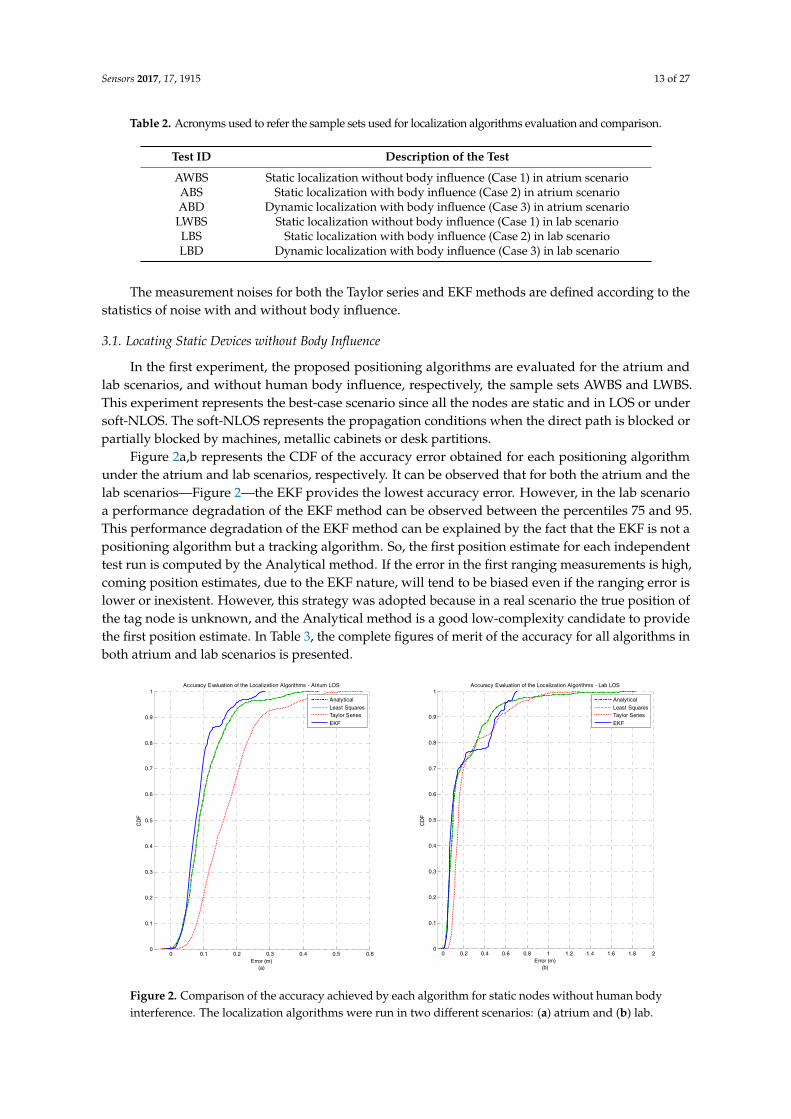
Table 2. Acronyms used to refer the sample sets used for localization algorithms evaluation and comparison.
Test ID Description of the Test
AWBS Static localization without body influence (Case 1) in atrium scenarioABS Static localization with body influence (Case 2) in atrium scenarioABD Dynamic localization with body influence (Case 3) in atrium scenario
LWBS Static localization without body influence (Case 1) in lab scenarioLBS Static localization with body influence (Case 2) in lab scenarioLBD Dynamic localization with body influence (Case 3) in lab scenario
The measurement noises for both the Taylor series and EKF methods are defined according to thestatistics of noise with and without body influence.
3.1. Locating Static Devices without Body Influence
In the first experiment, the proposed positioning algorithms are evaluated for the atrium andlab scenarios, and without human body influence, respectively, the sample sets AWBS and LWBS.This experiment represents the best-case scenario since all the nodes are static and in LOS or undersoft-NLOS. The soft-NLOS represents the propagation conditions when the direct path is blocked orpartially blocked by machines, metallic cabinets or desk partitions.
Figure 2a,b represents the CDF of the accuracy error obtained for each positioning algorithmunder the atrium and lab scenarios, respectively. It can be observed that for both the atrium and thelab scenarios—Figure 2—the EKF provides the lowest accuracy error. However, in the lab scenarioa performance degradation of the EKF method can be observed between the percentiles 75 and 95.This performance degradation of the EKF method can be explained by the fact that the EKF is not apositioning algorithm but a tracking algorithm. So, the first position estimate for each independenttest run is computed by the Analytical method. If the error in the first ranging measurements is high,coming position estimates, due to the EKF nature, will tend to be biased even if the ranging error islower or inexistent. However, this strategy was adopted because in a real scenario the true position ofthe tag node is unknown, and the Analytical method is a good low-complexity candidate to providethe first position estimate. In Table 3, the complete figures of merit of the accuracy for all algorithms inboth atrium and lab scenarios is presented.
Sensors 2017, 17, 1915 13 of 27
Figure 2a,b represent the CDF of the accuracy error obtained for each positioning algorithm under the atrium and lab scenarios, respectively. It can be observed that for both the atrium and the lab scenarios—Figure 2—the EKF provides the lowest accuracy error. However, in the lab scenario a performance degradation of the EKF method can be observed between the percentiles 75 and 95. This performance degradation of the EKF method can be explained by the fact that the EKF is not a positioning algorithm but a tracking algorithm. So, the first position estimate for each independent test run is computed by the Analytical method. If the error in the first ranging measurements is high, coming position estimates, due to the EKF nature, will tend to be biased even if the ranging error is lower or inexistent. However, this strategy was adopted because in a real scenario the true position of the tag node is unknown, and the Analytical method is a good low-complexity candidate to provide the first position estimate. In Table 3, the complete figures of merit of the accuracy for all algorithms in both atrium and lab scenarios is presented.
Figure 2. Comparison of the accuracy achieved by each algorithm for static nodes without human body interference. The localization algorithms were run in two different scenarios: (a) atrium and (b) lab.
Table 3. Performance comparison of the localization algorithms for the metrics accuracy, precision, and RMSE. All localization algorithms are compared for both atrium and lab scenarios and without human body interference.
Scenario Accuracy (m) Precision (m) RMSE (m)
0 50 90 95 99 100 0 50 90 95 99 100 RMSEx RMSEy Net RMSEAnalytic Method
AWBS 0 0.09 0.18 0.22 0.36 0.42 0 0.02 0.05 0.06 0.08 0.15 0.11 0.05 0.12 LWBS 0 0.09 0.45 0.56 1.22 1.81 0 0.03 0.08 0.23 0.72 1.18 0.19 0.22 0.29
Least Squares MethodAWBS 0 0.09 0.18 0.22 0.36 0.42 0 0.02 0.05 0.06 0.08 0.15 0.11 0.05 0.12 LWBS 0 0.09 0.45 0.56 1.22 1.81 0 0.03 0.08 0.23 0.72 1.18 0.19 0.22 0.29
Taylor Series MethodAWBS 0.02 0.16 0.27 0.37 0.46 0.54 0 0.02 0.04 0.05 0.06 0.18 0.17 0.09 0.19 LWBS 0.02 0.14 0.53 0.7 0.96 1.26 0 0.02 0.07 0.21 0.49 1.14 0.23 0.21 0.31
EKF MethodAWBS 0 0.08 0.16 0.2 0.26 0.27 0 0 0.01 0.03 0.06 0.21 0.09 0.04 0.1 LWBS 0.02 0.08 0.52 0.59 0.68 0.68 0 0 0.02 0.03 0.14 0.64 0.17 0.21 0.28
Figure 3a,b represent the CDF of the precision error obtained for each positioning algorithm under atrium and lab scenarios, respectively. For both scenarios, the EKF method outperforms the
0 0.1 0.2 0.3 0.4 0.5 0.60
0.1
0.2
0.3
0.4
0.5
0.6
0.7
0.8
0.9
1
Error (m)(a)
CD
F
Accuracy Evaluation of the Localization Algorithms - Atrium LOS
AnalyticalLeast SquaresTaylor SeriesEKF
0 0.2 0.4 0.6 0.8 1 1.2 1.4 1.6 1.8 20
0.1
0.2
0.3
0.4
0.5
0.6
0.7
0.8
0.9
1
Error (m)(b)
CD
F
Accuracy Evaluation of the Localization Algorithms - Lab LOS
AnalyticalLeast SquaresTaylor SeriesEKF
Figure 2. Comparison of the accuracy achieved by each algorithm for static nodes without human bodyinterference. The localization algorithms were run in two different scenarios: (a) atrium and (b) lab.

Sensors 2017, 17, 1915 14 of 27
Table 3. Performance comparison of the localization algorithms for the metrics accuracy, precision, andRMSE. All localization algorithms are compared for both atrium and lab scenarios and without humanbody interference.
ScenarioAccuracy (m) Precision (m) RMSE (m)
0 50 90 95 99 100 0 50 90 95 99 100 RMSEx RMSEy Net RMSEAnalytic Method
AWBS 0 0.09 0.18 0.22 0.36 0.42 0 0.02 0.05 0.06 0.08 0.15 0.11 0.05 0.12LWBS 0 0.09 0.45 0.56 1.22 1.81 0 0.03 0.08 0.23 0.72 1.18 0.19 0.22 0.29
Least Squares MethodAWBS 0 0.09 0.18 0.22 0.36 0.42 0 0.02 0.05 0.06 0.08 0.15 0.11 0.05 0.12LWBS 0 0.09 0.45 0.56 1.22 1.81 0 0.03 0.08 0.23 0.72 1.18 0.19 0.22 0.29
Taylor Series MethodAWBS 0.02 0.16 0.27 0.37 0.46 0.54 0 0.02 0.04 0.05 0.06 0.18 0.17 0.09 0.19LWBS 0.02 0.14 0.53 0.7 0.96 1.26 0 0.02 0.07 0.21 0.49 1.14 0.23 0.21 0.31
EKF MethodAWBS 0 0.08 0.16 0.2 0.26 0.27 0 0 0.01 0.03 0.06 0.21 0.09 0.04 0.1LWBS 0.02 0.08 0.52 0.59 0.68 0.68 0 0 0.02 0.03 0.14 0.64 0.17 0.21 0.28
Figure 3a,b represents the CDF of the precision error obtained for each positioning algorithmunder atrium and lab scenarios, respectively. For both scenarios, the EKF method outperforms theother algorithms in terms of precision. As expected, the Taylor series method also shows a betterperformance when compared with the Least Squares and Analytical methods, +33% for the atriumand +46% for the lab. In Table 3, the complete figures of merit of the precision for all algorithms inboth atrium and lab scenarios is presented.
Sensors 2017, 17, 1915 14 of 27
other algorithms in terms of precision. As expected, the Taylor series method also shows a better performance when compared with the Least Squares and Analytical methods, +33% for the atrium and +46% for the lab. In Table 3, the complete figures of merit of the precision for all algorithms in both atrium and lab scenarios is presented.
Figure 3. Comparison of the precision achieved by each algorithm for static nodes without human body interference. The localization algorithms were run in two different scenarios: (a) atrium and (b) lab.
Regarding the RMSE metric, the EKF method also performs better than the other algorithms for both scenarios. An interesting observation that can be made based on the RMSE metric is that the performance improvement of the EKF method is significantly higher for the atrium scenario (+20% and +90%) than in the lab scenario (+3% and +10%). This can be explained by the fact that the used noise statistics in the EKF were acquired in a corridor (free space area). Therefore, the atrium scenario best represents the used noise statistics of the signal than the lab scenario (where the signal propagation is under the influence of reflections, multipath and soft-NLOS phenomena). For the atrium scenario and for all algorithms, the X component of the RMSE is the predominant source of error in the net RMSE. On the other hand, for the lab scenario, the magnitude of both X and Y components are similar, but the Y component degrades up to 425% (for the EKF) whereas the X component degradation is 88% (also for the EKF). This increase in the RMSE of the Y component can be explained by the obstacles that create the soft-NLOS scenarios (machines, metallic cabinets or desk partitions), which are predominant in the Y axis. The Taylor Series is the method that experiences the lowest performance degradation when comparing both scenarios. However, it is also the method with the worst performance in both scenarios. The complete results for the RMSE metric can be consulted in Table 3.
Figures 4 and 5 illustrate the position estimates of each algorithm for atrium and lab scenarios, respectively. Through the analysis of both pictures, it is possible to confirm the gain in accuracy and more clearly in precision that the EKF has, in both scenario, when compared with the other positioning algorithms. The gain in precision is even more evident in the points where the ranging measurements are noisier (0 to 3 m in the X axis and 5 to 7 m in the Y axis, Figure 5). These points represent the soft-NLOS scenarios. From 0 to 3 m—in the X axis—the link anchor-tag is blocked by a metallic cabinet and from 5 to 7 m—in the Y axis—the link anchor-tag is blocked by a desk partition. In Figure 5 we can also see the positive bias created by the metallic cabinet.
-0.05 0 0.05 0.1 0.150
0.1
0.2
0.3
0.4
0.5
0.6
0.7
0.8
0.9
1
Error (m)(a)
CD
F
Precision Evaluation of the Localization Algorithms - Atrium LOS
AnalyticalLeast SquaresTaylor SeriesEKF
0 0.2 0.4 0.6 0.8 1 1.20
0.1
0.2
0.3
0.4
0.5
0.6
0.7
0.8
0.9
1
Error (m)(b)
CD
F
Precision Evaluation of the Localization Algorithms - Lab LOS
AnalyticalLeast SquaresTaylor SeriesEKF
Figure 3. Comparison of the precision achieved by each algorithm for static nodes without human bodyinterference. The localization algorithms were run in two different scenarios: (a) atrium and (b) lab.
Regarding the RMSE metric, the EKF method also performs better than the other algorithms forboth scenarios. An interesting observation that can be made based on the RMSE metric is that theperformance improvement of the EKF method is significantly higher for the atrium scenario (+20% and+90%) than in the lab scenario (+3% and +10%). This can be explained by the fact that the used noisestatistics in the EKF were acquired in a corridor (free space area). Therefore, the atrium scenario bestrepresents the used noise statistics of the signal than the lab scenario (where the signal propagation isunder the influence of reflections, multipath and soft-NLOS phenomena). For the atrium scenario andfor all algorithms, the X component of the RMSE is the predominant source of error in the net RMSE.On the other hand, for the lab scenario, the magnitude of both X and Y components are similar, but theY component degrades up to 425% (for the EKF) whereas the X component degradation is 88% (alsofor the EKF). This increase in the RMSE of the Y component can be explained by the obstacles thatcreate the soft-NLOS scenarios (machines, metallic cabinets or desk partitions), which are predominant

Sensors 2017, 17, 1915 15 of 27
in the Y axis. The Taylor Series is the method that experiences the lowest performance degradationwhen comparing both scenarios. However, it is also the method with the worst performance in bothscenarios. The complete results for the RMSE metric can be consulted in Table 3.
Figures 4 and 5 illustrate the position estimates of each algorithm for atrium and lab scenarios,respectively. Through the analysis of both pictures, it is possible to confirm the gain in accuracy andmore clearly in precision that the EKF has, in both scenario, when compared with the other positioningalgorithms. The gain in precision is even more evident in the points where the ranging measurementsare noisier (0 to 3 m in the X axis and 5 to 7 m in the Y axis, Figure 5). These points represent thesoft-NLOS scenarios. From 0 to 3 m—in the X axis—the link anchor-tag is blocked by a metallic cabinetand from 5 to 7 m—in the Y axis—the link anchor-tag is blocked by a desk partition. In Figure 5 wecan also see the positive bias created by the metallic cabinet.
Sensors 2017, 17, 1915 15 of 27
Figure 4. Graphical illustration of the 200 position estimates per test point in the atrium scenario and without human body interference. (a) Analytical method; (b) Least Squares method; (c) Taylor Series Method; and (d) EKF Method.
Figure 5. Graphical illustration of the 200 position estimates for each test point in the lab scenario and without human body interference. (a) Analytical method; (b) Least Squares method; (c) Taylor Series Method; and (d) EKF Method.
3.2. Locating Static Devices with Body Influence
In the second experiment, the proposed positioning algorithms are evaluated for the same scenarios, but under the human body influence. In this evaluation, the positioning algorithms are run with the samples sets ABS and LBS for the Atrium and Lab scenarios, respectively. Additionally, the performance of the positioning algorithms is also evaluated when the NLOS identification and mitigation algorithm (proposed in Section 2.2) is applied for the ranging measurements, whose tag-anchor link is under the body influence.
0 1 2 3 4 5 6 70
2
4
6
8
102D Position estimation results: Analytical Method - Atrium LOS
X (m)(a)
Y (
m)
Estimated positionAnchor Nodes PositionTrue Position
0 1 2 3 4 5 6 70
2
4
6
8
102D Position estimation results: Least Squares Method - Atrium LOS
X (m)(b)
Y (
m)
Estimated positionAnchor Nodes PositionTrue Position
0 1 2 3 4 5 6 70
2
4
6
8
102D Position estimation results: Taylor Series Method - Atrium LOS
X (m)(c)
Y (m
)
Estimated positionAnchor Nodes PositionTrue Position
0 1 2 3 4 5 6 70
2
4
6
8
102D Position estimation results: EKF Method - Atrium LOS
X (m)(d)
Y (m
)
Estimated positionAnchor Nodes PositionTrue Position
0 1 2 3 4 5 6 7 8 9 100
1
2
3
4
5
6
7
82D Position estimation results: Analytical Method - Lab LOS
X (m)(a)
Y (
m)
Estimated positionAnchor Nodes PositionTrue Position
0 1 2 3 4 5 6 7 8 9 100
1
2
3
4
5
6
7
82D Position estimation results: Least Squares Method - Lab LOS
X (m)(b)
Y (
m)
Estimated positionAnchor Nodes PositionTrue Position
0 1 2 3 4 5 6 7 8 9 100
1
2
3
4
5
6
7
82D Position estimation results: Taylor Series Method - Lab LOS
X (m)(c)
Y (
m)
Estimated positionAnchor Nodes PositionTrue Position
0 1 2 3 4 5 6 7 8 9 100
1
2
3
4
5
6
72D Position estimation results: EKF Method - Lab LOS
X (m)(d)
Y (
m)
Estimated positionAnchor Nodes PositionTrue Position
Figure 4. Graphical illustration of the 200 position estimates per test point in the atrium scenario andwithout human body interference. (a) Analytical method; (b) Least Squares method; (c) Taylor SeriesMethod; and (d) EKF Method.
Sensors 2017, 17, 1915 15 of 27
Figure 4. Graphical illustration of the 200 position estimates per test point in the atrium scenario and without human body interference. (a) Analytical method; (b) Least Squares method; (c) Taylor Series Method; and (d) EKF Method.
Figure 5. Graphical illustration of the 200 position estimates for each test point in the lab scenario and without human body interference. (a) Analytical method; (b) Least Squares method; (c) Taylor Series Method; and (d) EKF Method.
3.2. Locating Static Devices with Body Influence
In the second experiment, the proposed positioning algorithms are evaluated for the same scenarios, but under the human body influence. In this evaluation, the positioning algorithms are run with the samples sets ABS and LBS for the Atrium and Lab scenarios, respectively. Additionally, the performance of the positioning algorithms is also evaluated when the NLOS identification and mitigation algorithm (proposed in Section 2.2) is applied for the ranging measurements, whose tag-anchor link is under the body influence.
0 1 2 3 4 5 6 70
2
4
6
8
102D Position estimation results: Analytical Method - Atrium LOS
X (m)(a)
Y (
m)
Estimated positionAnchor Nodes PositionTrue Position
0 1 2 3 4 5 6 70
2
4
6
8
102D Position estimation results: Least Squares Method - Atrium LOS
X (m)(b)
Y (
m)
Estimated positionAnchor Nodes PositionTrue Position
0 1 2 3 4 5 6 70
2
4
6
8
102D Position estimation results: Taylor Series Method - Atrium LOS
X (m)(c)
Y (m
)
Estimated positionAnchor Nodes PositionTrue Position
0 1 2 3 4 5 6 70
2
4
6
8
102D Position estimation results: EKF Method - Atrium LOS
X (m)(d)
Y (m
)
Estimated positionAnchor Nodes PositionTrue Position
0 1 2 3 4 5 6 7 8 9 100
1
2
3
4
5
6
7
82D Position estimation results: Analytical Method - Lab LOS
X (m)(a)
Y (
m)
Estimated positionAnchor Nodes PositionTrue Position
0 1 2 3 4 5 6 7 8 9 100
1
2
3
4
5
6
7
82D Position estimation results: Least Squares Method - Lab LOS
X (m)(b)
Y (
m)
Estimated positionAnchor Nodes PositionTrue Position
0 1 2 3 4 5 6 7 8 9 100
1
2
3
4
5
6
7
82D Position estimation results: Taylor Series Method - Lab LOS
X (m)(c)
Y (
m)
Estimated positionAnchor Nodes PositionTrue Position
0 1 2 3 4 5 6 7 8 9 100
1
2
3
4
5
6
72D Position estimation results: EKF Method - Lab LOS
X (m)(d)
Y (
m)
Estimated positionAnchor Nodes PositionTrue Position
Figure 5. Graphical illustration of the 200 position estimates for each test point in the lab scenario andwithout human body interference. (a) Analytical method; (b) Least Squares method; (c) Taylor SeriesMethod; and (d) EKF Method.

Sensors 2017, 17, 1915 16 of 27
3.2. Locating Static Devices with Body Influence
In the second experiment, the proposed positioning algorithms are evaluated for the samescenarios, but under the human body influence. In this evaluation, the positioning algorithms arerun with the samples sets ABS and LBS for the Atrium and Lab scenarios, respectively. Additionally,the performance of the positioning algorithms is also evaluated when the NLOS identification andmitigation algorithm (proposed in Section 2.2) is applied for the ranging measurements, whosetag-anchor link is under the body influence.
The CDFs of the accuracy error under human body influence, in both atrium and lab scenarios,and with or without NLOS mitigation are illustrated in Figure 6. It can also be seen that the EKFmethod provides the lowest accuracy error for the majority of the scenarios studied. The only exceptionoccurs when the EKF is combined with the NLOS mitigation algorithm in the lab scenario. For thisscenario, the performance of the EKF method degrades after 85th percentile, making its performanceworse than without NLOS mitigation algorithm and worse than the other three positioning algorithms.Another interesting observation is that unlike the other methods, the performance of the EKF in the99th percentile is better in the atrium (0.7 m with NLOS mitigation and) than the lab (1.77 m withoutNLOS mitigation). The NLOS mitigation algorithm proposed in Section 2.2 proved to successfullyimprove the localization accuracy. This improvement in accuracy was more significant for the analyticaland least squares methods. However, this error reduction is more evident for lower probabilities.The Taylor Series method showed the worst performance in both scenarios and with or without NLOSmitigation for the 99th percentile. In Table 4, the complete figures of merit of the accuracy for allalgorithms in both atrium and lab scenarios and with or without NLOS mitigation is presented.
Sensors 2017, 17, 1915 16 of 27
The CDFs of the accuracy error under human body influence, in both atrium and lab scenarios, and with or without NLOS mitigation are illustrated in Figure 6. It can also be seen that the EKF method provides the lowest accuracy error for the majority of the scenarios studied. The only exception occurs when the EKF is combined with the NLOS mitigation algorithm in the lab scenario. For this scenario, the performance of the EKF method degrades after 85th percentile, making its performance worse than without NLOS mitigation algorithm and worse than the other three positioning algorithms. Another interesting observation is that unlike the other methods, the performance of the EKF in the 99th percentile is better in the atrium (0.7 m with NLOS mitigation and) than the lab (1.77 m without NLOS mitigation). The NLOS mitigation algorithm proposed in Section 2.2 proved to successfully improve the localization accuracy. This improvement in accuracy was more significant for the analytical and least squares methods. However, this error reduction is more evident for lower probabilities. The Taylor Series method showed the worst performance in both scenarios and with or without NLOS mitigation for the 99th percentile. In Table 4, the complete figures of merit of the accuracy for all algorithms in both atrium and lab scenarios and with or without NLOS mitigation is presented.
Figure 6. Comparison of the accuracy achieved by each algorithm for static nodes with human body interference and with or without NLOS mitigation. The first row represents the accuracy achieved by each algorithm in atrium with (a) and without (b) NLOS mitigation. Whereas, the second row represents the accuracy achieved by each algorithm in lab with (c) and without (d) NLOS mitigation.
0 0.5 1 1.5 2 2.5 3 3.50
0.2
0.4
0.6
0.8
1
Error (m)(a)
CD
F
Accuracy Evaluation of the Localization Algorithms - Atrium Body
AnalyticalLeast SquaresTaylor SeriesEKF
0 0.5 1 1.5 2 2.5 3 3.50
0.2
0.4
0.6
0.8
1
Error (m)(b)
CD
F
Accuracy Evaluation of the Localization Algorithms - Atrium Body with NLOS Mitigation
AnalyticalLeast SquaresTaylor SeriesEKF
0 0.5 1 1.5 2 2.5 3 3.50
0.2
0.4
0.6
0.8
1
Error (m)(c)
CD
F
Accuracy Evaluation of the Localization Algorithms - Lab Body
AnalyticalLeast SquaresTaylor SeriesEKF
0 0.5 1 1.5 2 2.5 3 3.50
0.2
0.4
0.6
0.8
1
Error (m)(d)
CD
F
Accuracy Evaluation of the Localization Algorithms - Lab Body with NLOS Mitigation
AnalyticalLeast SquaresTaylor SeriesEKF
Figure 6. Comparison of the accuracy achieved by each algorithm for static nodes with human bodyinterference and with or without NLOS mitigation. The first row represents the accuracy achievedby each algorithm in atrium with (a) and without (b) NLOS mitigation. Whereas, the second rowrepresents the accuracy achieved by each algorithm in lab with (c) and without (d) NLOS mitigation.

Sensors 2017, 17, 1915 17 of 27
Table 4. Performance comparison of the localization algorithms for the metrics accuracy, precision, andRMSE. All localization algorithms are compared for both atrium and lab scenarios, with human bodyinterference, and with or without NLOS mitigation algorithm.
ScenarioAccuracy (m) Precision (m) RMSE (m)
0 50 90 95 99 100 0 50 90 95 99 100 RMSEx RMSEy Net RMSEAnalytic Method
ABS 0.01 0.79 1.78 2.12 3.13 4.7 0 0.09 0.73 0.94 1.5 2.82 0.08 1.14 1.14ABS_M 0 0.46 1.3 1.63 2.61 3.9 0 0.08 0.65 0.85 1.31 2.45 0.07 0.81 0.81
LBS 0.01 0.56 1.37 1.62 2.13 2.95 0 0.1 0.62 0.81 1.46 2.02 0.7 0.42 0.82LBS_M 0 0.39 1.01 1.33 2.02 2.98 0 0.1 0.58 0.74 1.28 1.79 0.49 0.41 0.64
Least Squares MethodABS 0.01 0.79 1.78 2.12 3.13 4.7 0 0.09 0.73 0.94 1.5 2.82 0.08 1.14 1.14
ABS_M 0 0.46 1.3 1.63 2.61 3.9 0 0.08 0.65 0.85 1.31 2.45 0.07 0.81 0.81LBS 0.01 0.56 1.37 1.62 2.13 2.95 0 0.1 0.62 0.81 1.46 2.02 0.7 0.42 0.82
LBS_M 0 0.39 1.01 1.33 2.02 2.98 0 0.1 0.58 0.74 1.28 1.79 0.49 0.41 0.64Taylor Series Method
ABS 0.04 0.69 1.61 1.74 3.38 6.56 0 0.08 0.6 0.91 2.4 5.83 0.61 0.88 1.07ABS_M 0 0.67 1.72 2.07 3.17 4.83 0 0.12 0.88 1.18 1.6 4.43 0.71 0.84 1.1
LBS 0 0.43 1.36 1.99 3.14 3.67 0 0.09 0.59 0.78 1.82 2.9 0.6 0.65 0.88LBS_M 0 0.3 1.13 1.59 2.92 3.42 0 0.09 0.53 0.72 1.49 2.97 0.49 0.55 0.73
EKF MethodABS 0.02 0.12 0.31 0.96 1.18 1.19 0 0.01 0.04 0.06 0.19 0.76 0.08 0.31 0.32
ABS_M 0.01 0.16 0.52 0.61 0.7 1.01 0 0.01 0.04 0.07 0.19 0.56 0.15 0.24 0.28LBS 0.01 0.36 0.87 1.16 1.77 1.78 0 0.02 0.13 0.19 0.49 1.79 0.34 0.47 0.58
LBS_M 0 0.2 1.22 1.56 1.85 1.86 0 0.02 0.07 0.13 0.38 1.71 0.42 0.4 0.58
The CDFs of the precision error under human body influence, in both atrium and lab scenarios,and with or without NLOS mitigation are illustrated in Figure 7. The best performance for bothscenarios is achieved by the EKF method when the NLOS mitigation algorithm is run. For the atriumscenario no improvement is observed when the NLOS mitigation algorithm is applied whereas inthe lab scenario an improvement of 29% is observed. In Table 4, the complete figures of merit of theprecision for all algorithms in both atrium and lab scenarios, and with or without NLOS mitigationis presented.
Sensors 2017, 17, 1915 17 of 27
Table 4. Performance comparison of the localization algorithms for the metrics accuracy, precision, and RMSE. All localization algorithms are compared for both atrium and lab scenarios, with human body interference, and with or without NLOS mitigation algorithm.
Scenario Accuracy (m) Precision (m) RMSE (m)
0 50 90 95 99 100 0 50 90 95 99 100 RMSEx RMSEy Net RMSEAnalytic Method
ABS 0.01 0.79 1.78 2.12 3.13 4.7 0 0.09 0.73 0.94 1.5 2.82 0.08 1.14 1.14 ABS_M 0 0.46 1.3 1.63 2.61 3.9 0 0.08 0.65 0.85 1.31 2.45 0.07 0.81 0.81
LBS 0.01 0.56 1.37 1.62 2.13 2.95 0 0.1 0.62 0.81 1.46 2.02 0.7 0.42 0.82 LBS_M 0 0.39 1.01 1.33 2.02 2.98 0 0.1 0.58 0.74 1.28 1.79 0.49 0.41 0.64
Least Squares MethodABS 0.01 0.79 1.78 2.12 3.13 4.7 0 0.09 0.73 0.94 1.5 2.82 0.08 1.14 1.14
ABS_M 0 0.46 1.3 1.63 2.61 3.9 0 0.08 0.65 0.85 1.31 2.45 0.07 0.81 0.81 LBS 0.01 0.56 1.37 1.62 2.13 2.95 0 0.1 0.62 0.81 1.46 2.02 0.7 0.42 0.82
LBS_M 0 0.39 1.01 1.33 2.02 2.98 0 0.1 0.58 0.74 1.28 1.79 0.49 0.41 0.64 Taylor Series Method
ABS 0.04 0.69 1.61 1.74 3.38 6.56 0 0.08 0.6 0.91 2.4 5.83 0.61 0.88 1.07 ABS_M 0 0.67 1.72 2.07 3.17 4.83 0 0.12 0.88 1.18 1.6 4.43 0.71 0.84 1.1
LBS 0 0.43 1.36 1.99 3.14 3.67 0 0.09 0.59 0.78 1.82 2.9 0.6 0.65 0.88 LBS_M 0 0.3 1.13 1.59 2.92 3.42 0 0.09 0.53 0.72 1.49 2.97 0.49 0.55 0.73
EKF MethodABS 0.02 0.12 0.31 0.96 1.18 1.19 0 0.01 0.04 0.06 0.19 0.76 0.08 0.31 0.32
ABS_M 0.01 0.16 0.52 0.61 0.7 1.01 0 0.01 0.04 0.07 0.19 0.56 0.15 0.24 0.28 LBS 0.01 0.36 0.87 1.16 1.77 1.78 0 0.02 0.13 0.19 0.49 1.79 0.34 0.47 0.58
LBS_M 0 0.2 1.22 1.56 1.85 1.86 0 0.02 0.07 0.13 0.38 1.71 0.42 0.4 0.58
The CDFs of the precision error under human body influence, in both atrium and lab scenarios, and with or without NLOS mitigation are illustrated in Figure 7. The best performance for both scenarios is achieved by the EKF method when the NLOS mitigation algorithm is run. For the atrium scenario no improvement is observed when the NLOS mitigation algorithm is applied whereas in the lab scenario an improvement of 29% is observed. In Table 4, the complete figures of merit of the precision for all algorithms in both atrium and lab scenarios, and with or without NLOS mitigation is presented.
Figure 7. Comparison of the precision achieved by each algorithm for static nodes with human body interference and with or without NLOS mitigation. The first row represents the precision achieved by each algorithm in atrium with (a) and without (b) NLOS mitigation. Whereas, the second row represents the precision achieved by each algorithm in lab with (c) and without (d) NLOS mitigation.
0 0.5 1 1.50
0.2
0.4
0.6
0.8
1
Error (m)(a)
CD
F
Precision Evaluation of the Localization Algorithms - Atrium Body
AnalyticalLeast SquaresTaylor SeriesEKF
0 0.5 1 1.50
0.2
0.4
0.6
0.8
1
Error (m)(b)
CD
F
Precision Evaluation of the Localization Algorithms - Atrium Body with NLOS Mitigation
AnalyticalLeast SquaresTaylor SeriesEKF
0 0.5 1 1.50
0.2
0.4
0.6
0.8
1
Error (m)(c)
CD
F
Precision Evaluation of the Localization Algorithms - Lab Body
AnalyticalLeast SquaresTaylor SeriesEKF
0 0.5 1 1.50
0.2
0.4
0.6
0.8
1
Error (m)(d)
CD
F
Precision Evaluation of the Localization Algorithms - Lab Body with NLOS Mitigation
AnalyticalLeast SquaresTaylor SeriesEKF
Figure 7. Comparison of the precision achieved by each algorithm for static nodes with human bodyinterference and with or without NLOS mitigation. The first row represents the precision achievedby each algorithm in atrium with (a) and without (b) NLOS mitigation. Whereas, the second rowrepresents the precision achieved by each algorithm in lab with (c) and without (d) NLOS mitigation.

Sensors 2017, 17, 1915 18 of 27
Regarding the RMSE metric, the EKF method also outperforms the other methods in bothscenarios. The net RMSE of all methods decreases when the NLOS mitigation is used. The onlyexception occurs with the Taylor Series method in the atrium, where the net RMSE slightly increased.Like in the previous experiment, the performance improvement of the EKF method is significantlyhigher for the atrium scenario. However, in this experiment is the Y component of the RMSE that is thepredominant source of error in the net RMSE for the atrium. This happens because of the orientationof the human body during the measurement campaign, leading an error propagation in the Y axis.For the lab scenario, the magnitudes of X and Y components are similar. The complete results for theRMSE metric can be consulted in Table 4.
Figures 8 and 9 illustrate the position estimates of each algorithm with and without NLOSmitigation for atrium and lab scenarios, respectively. Through the analysis of both pictures, it is possibleto confirm the gain in accuracy and more clearly in precision that EKF has, in both scenarios, whencompared with the other positioning algorithms. Another interesting observation is the propagation ofthe ranging error due to the human body influence. From the analysis of both figures, especially forAnalytical and Least Squares methods, it is possible to observe that the orientation of the human bodyhas a clear effect on the error propagation. For the atrium scenario, the human body is perpendicularto the Y axis and the position error propagates in that direction. On the other hand, for the lab scenario,the human body is perpendicular to the X axis and the position error also propagates in that direction.
Sensors 2017, 17, 1915 18 of 27
Regarding the RMSE metric, the EKF method also outperforms the other methods in both scenarios. The net RMSE of all methods decreases when the NLOS mitigation is used. The only exception occurs with the Taylor Series method in the atrium, where the net RMSE slightly increased. Like in the previous experiment, the performance improvement of the EKF method is significantly higher for the atrium scenario. However, in this experiment is the Y component of the RMSE that is the predominant source of error in the net RMSE for the atrium. This happens because of the orientation of the human body during the measurement campaign, leading an error propagation in the Y axis. For the lab scenario, the magnitudes of X and Y components are similar. The complete results for the RMSE metric can be consulted in Table 4.
Figures 8 and 9 illustrate the position estimates of each algorithm with and without NLOS mitigation for atrium and lab scenarios, respectively. Through the analysis of both pictures, it is possible to confirm the gain in accuracy and more clearly in precision that EKF has, in both scenarios, when compared with the other positioning algorithms. Another interesting observation is the propagation of the ranging error due to the human body influence. From the analysis of both figures, especially for Analytical and Least Squares methods, it is possible to observe that the orientation of the human body has a clear effect on the error propagation. For the atrium scenario, the human body is perpendicular to the Y axis and the position error propagates in that direction. On the other hand, for the lab scenario, the human body is perpendicular to the X axis and the position error also propagates in that direction.
Figure 8. Graphical illustration of the 200 position estimates for each test point in the atrium scenario, with human body interference, and with or without NLOS mitigation. The plots on the left side of the figure represent the position estimates without NLOS mitigation and the plots on the right the position estimates with NLOS mitigation. Each row represents the results obtained by each positioning algorithm and their order from the top to the bottom of the figure is: Analytical method —(a,b); Least Squares method—(c,d); Taylor Series method—(e,f); and EKF Method—(g,h).
0 1 2 3 4 5 6 70
5
10
152D Position estimation results: Analytical Method - Atrium Body
X (m)(a)
Y (m
)
0 1 2 3 4 5 6 70
5
102D Position estimation results: Analytical Method - Atrium Body with NLOS Mitigation
X (m)(b)
Y (m
)
0 1 2 3 4 5 6 70
5
10
152D Position estimation results: Least Squares Method - Atrium Body
X (m)(c)
Y (
m)
0 1 2 3 4 5 6 70
5
102D Position estimation results: Least Squares Method - Atrium Body with NLOS Mitigation
X (m)(d)
Y (
m)
-1 0 1 2 3 4 5 6 7 80
5
10
152D Position estimation results: Taylor Series Method - Atrium Body
X (m)(e)
Y (m
)
Estimated positionAnchor Nodes PositionTrue Position
-2 -1 0 1 2 3 4 5 6 7 80
5
10
152D Position estimation results: Taylor Series Method - Atrium Body with NLOS Mitigation
X (m)(f)
Y (m
)
0 1 2 3 4 5 6 70
5
102D Position estimation results: EKF Method - Atrium Body
X (m)(g)
Y (m
)
0 1 2 3 4 5 6 70
5
102D Position estimation results: EKF Method - Atrium Body with NLOS Mitigation
X (m)(h)
Y (m
)
Figure 8. Graphical illustration of the 200 position estimates for each test point in the atrium scenario,with human body interference, and with or without NLOS mitigation. The plots on the left side ofthe figure represent the position estimates without NLOS mitigation and the plots on the right theposition estimates with NLOS mitigation. Each row represents the results obtained by each positioningalgorithm and their order from the top to the bottom of the figure is: Analytical method —(a,b); LeastSquares method—(c,d); Taylor Series method—(e,f); and EKF Method—(g,h).

Sensors 2017, 17, 1915 19 of 27Sensors 2017, 17, 1915 19 of 27
Figure 9. Graphical illustration of the 200 position estimates for each test point in the lab scenario, with human body interference, and with or without NLOS mitigation. The plots on the left side of the figure represent the position estimates without NLOS mitigation and the plots on the right the position estimates with NLOS mitigation. Each row represents the results obtained by each positioning algorithm and their order from the top to the bottom of the figure is: Analytical method —(a,b); Least Squares method—(c,d); Taylor Series method—(e,f); and EKF Method—(g,h).
3.3. Locating Mobile Devices with Body Influence
In the third experiment, the proposed positioning algorithms are evaluated for mobile devices and under human body influence. In this evaluation, the positioning algorithms are run with the samples sets ABD and LBD for the Atrium and Lab scenarios, respectively. As in the previous test, the performance of the positioning algorithms is also compared when the NLOS identification and mitigation algorithm (proposed in Section 2.2) is applied to improve the ranging measurements.
Figures 10–13 represent the position estimates and the user’s estimated path during the dynamic tests in atrium (Figures 10 and 11) and lab (Figures 12 and 13). On the left side of the figures (subplots a and c) are illustrated the position estimates without running the NLOS identification and error mitigation algorithm and, on the right side, the position estimates after running the NLOS identification and error mitigation algorithm (subplots b and d). For both scenarios, the walked path was designed so that the number of anchor nodes under NLOS condition varies between one and two. As can be seen from the figures, when two anchor nodes are in NLOS condition (green lines) the performance of all positioning algorithms severely deteriorates. When only one anchor node is under NLOS condition, the Analytical and the Least Squares methods perform better than the Taylor Series and the EKF methods. However, when the number of anchor nodes in NLOS condition increase, the performance of the Taylor Series and the EKF methods is higher. This is especially visible in the lab path where only the EKF method has a computed path close to the performed path. Another observation that can be drawn from the images is that the performance gain by running the NLOS identification and error mitigation algorithm is higher for the Taylor Series and EKF methods.
-2 0 2 4 6 8 100
5
102D Position estimation results: Analytical Method - Lab Body
X (m)(a)
Y (
m)
0 1 2 3 4 5 6 7 8 9 100
5
102D Position estimation results: Analytical Method - Lab Body with NLOS Mitigation
X (m)(b)
Y (
m)
-2 0 2 4 6 8 100
5
102D Position estimation results: Least Squares Method - Lab Body
X (m)(c)
Y (
m)
0 1 2 3 4 5 6 7 8 9 100
5
102D Position estimation results: Least Squares Method - Lab Body with NLOS Mitigation
X (m)(d)
Y (
m)
-2 0 2 4 6 8 10-5
0
5
102D Position estimation results: Taylor Series Method - Lab Body
X (m)(e)
Y (m
)
Estimated positionAnchor Nodes PositionTrue Position
-2 0 2 4 6 8 10-5
0
5
102D Position estimation results: Taylor Series Method - Lab Body with NLOS Mitigation
X (m)(f)
Y (m
)
0 1 2 3 4 5 6 7 8 9 100
5
102D Position estimation results: EKF Method - Lab Body
X (m)(g)
Y (
m)
0 1 2 3 4 5 6 7 8 9 100
5
102D Position estimation results: EKF Method - Lab Body with NLOS Mitigation
X (m)(h)
Y (
m)
Figure 9. Graphical illustration of the 200 position estimates for each test point in the lab scenario,with human body interference, and with or without NLOS mitigation. The plots on the left side ofthe figure represent the position estimates without NLOS mitigation and the plots on the right theposition estimates with NLOS mitigation. Each row represents the results obtained by each positioningalgorithm and their order from the top to the bottom of the figure is: Analytical method —(a,b); LeastSquares method—(c,d); Taylor Series method—(e,f); and EKF Method—(g,h).
3.3. Locating Mobile Devices with Body Influence
In the third experiment, the proposed positioning algorithms are evaluated for mobile devicesand under human body influence. In this evaluation, the positioning algorithms are run with thesamples sets ABD and LBD for the Atrium and Lab scenarios, respectively. As in the previous test,the performance of the positioning algorithms is also compared when the NLOS identification andmitigation algorithm (proposed in Section 2.2) is applied to improve the ranging measurements.
Figures 10–13 represent the position estimates and the user’s estimated path during the dynamictests in atrium (Figures 10 and 11) and lab (Figures 12 and 13). On the left side of the figures(subplots a and c) are illustrated the position estimates without running the NLOS identificationand error mitigation algorithm and, on the right side, the position estimates after running the NLOSidentification and error mitigation algorithm (subplots b and d). For both scenarios, the walked pathwas designed so that the number of anchor nodes under NLOS condition varies between one andtwo. As can be seen from the figures, when two anchor nodes are in NLOS condition (green lines) theperformance of all positioning algorithms severely deteriorates. When only one anchor node is underNLOS condition, the Analytical and the Least Squares methods perform better than the Taylor Seriesand the EKF methods. However, when the number of anchor nodes in NLOS condition increase, theperformance of the Taylor Series and the EKF methods is higher. This is especially visible in the lab pathwhere only the EKF method has a computed path close to the performed path. Another observationthat can be drawn from the images is that the performance gain by running the NLOS identificationand error mitigation algorithm is higher for the Taylor Series and EKF methods.
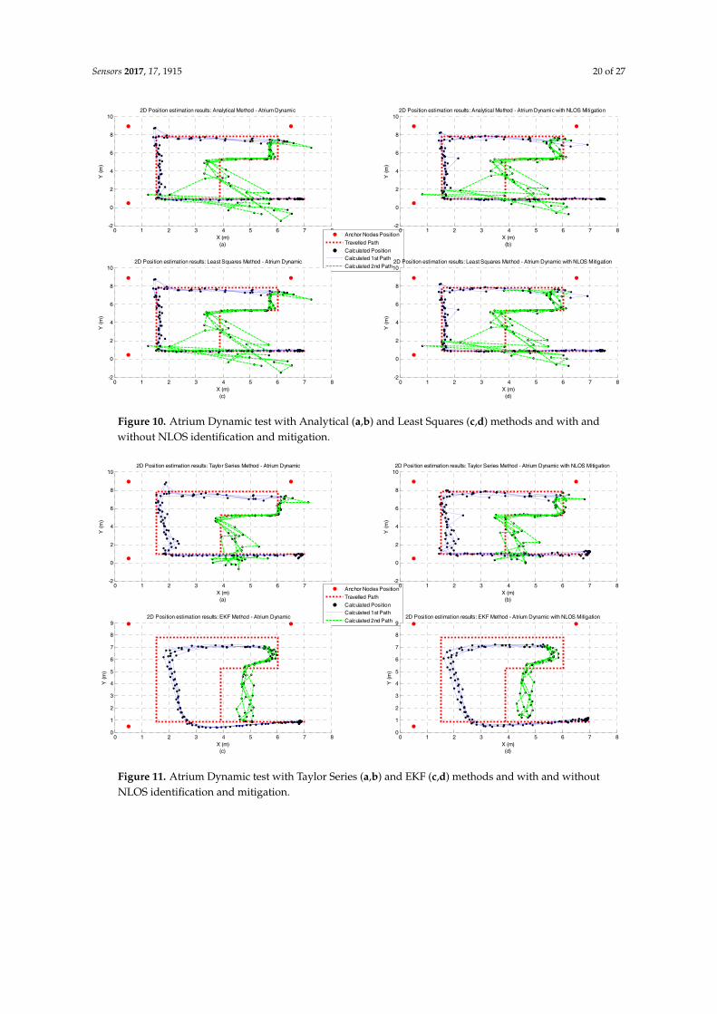
Sensors 2017, 17, 1915 20 of 27Sensors 2017, 17, 1915 20 of 27
Figure 10. Atrium Dynamic test with Analytical (a,b) and Least Squares (c,d) methods and with and without NLOS identification and mitigation.
Figure 11. Atrium Dynamic test with Taylor Series (a,b) and EKF (c,d) methods and with and without NLOS identification and mitigation.
0 1 2 3 4 5 6 7 8-2
0
2
4
6
8
102D Position estimation results: Analytical Method - Atrium Dynamic
X (m)(a)
Y (
m)
Anchor Nodes PositionTravelled PathCalculated PositionCalculated 1st PathCalculated 2nd Path
0 1 2 3 4 5 6 7 8-2
0
2
4
6
8
102D Position estimation results: Analytical Method - Atrium Dynamic with NLOS Mitigation
X (m)(b)
Y (
m)
0 1 2 3 4 5 6 7 8-2
0
2
4
6
8
102D Position estimation results: Least Squares Method - Atrium Dynamic
X (m)(c)
Y (
m)
0 1 2 3 4 5 6 7 8-2
0
2
4
6
8
102D Position estimation results: Least Squares Method - Atrium Dynamic with NLOS Mitigation
X (m)(d)
Y (
m)
0 1 2 3 4 5 6 7 8-2
0
2
4
6
8
102D Position estimation results: Taylor Series Method - Atrium Dynamic
X (m)(a)
Y (m
)
Anchor Nodes PositionTravelled PathCalculated PositionCalculated 1st PathCalculated 2nd Path
0 1 2 3 4 5 6 7 8-2
0
2
4
6
8
102D Position estimation results: Taylor Series Method - Atrium Dynamic with NLOS Mitigation
X (m)(b)
Y (m
)
0 1 2 3 4 5 6 7 80
1
2
3
4
5
6
7
8
92D Position estimation results: EKF Method - Atrium Dynamic
X (m)(c)
Y (
m)
0 1 2 3 4 5 6 7 80
1
2
3
4
5
6
7
8
92D Position estimation results: EKF Method - Atrium Dynamic with NLOS Mitigation
X (m)(d)
Y (
m)
Figure 10. Atrium Dynamic test with Analytical (a,b) and Least Squares (c,d) methods and with andwithout NLOS identification and mitigation.
Sensors 2017, 17, 1915 20 of 27
Figure 10. Atrium Dynamic test with Analytical (a,b) and Least Squares (c,d) methods and with and without NLOS identification and mitigation.
Figure 11. Atrium Dynamic test with Taylor Series (a,b) and EKF (c,d) methods and with and without NLOS identification and mitigation.
0 1 2 3 4 5 6 7 8-2
0
2
4
6
8
102D Position estimation results: Analytical Method - Atrium Dynamic
X (m)(a)
Y (
m)
Anchor Nodes PositionTravelled PathCalculated PositionCalculated 1st PathCalculated 2nd Path
0 1 2 3 4 5 6 7 8-2
0
2
4
6
8
102D Position estimation results: Analytical Method - Atrium Dynamic with NLOS Mitigation
X (m)(b)
Y (
m)
0 1 2 3 4 5 6 7 8-2
0
2
4
6
8
102D Position estimation results: Least Squares Method - Atrium Dynamic
X (m)(c)
Y (
m)
0 1 2 3 4 5 6 7 8-2
0
2
4
6
8
102D Position estimation results: Least Squares Method - Atrium Dynamic with NLOS Mitigation
X (m)(d)
Y (
m)
0 1 2 3 4 5 6 7 8-2
0
2
4
6
8
102D Position estimation results: Taylor Series Method - Atrium Dynamic
X (m)(a)
Y (m
)
Anchor Nodes PositionTravelled PathCalculated PositionCalculated 1st PathCalculated 2nd Path
0 1 2 3 4 5 6 7 8-2
0
2
4
6
8
102D Position estimation results: Taylor Series Method - Atrium Dynamic with NLOS Mitigation
X (m)(b)
Y (m
)
0 1 2 3 4 5 6 7 80
1
2
3
4
5
6
7
8
92D Position estimation results: EKF Method - Atrium Dynamic
X (m)(c)
Y (
m)
0 1 2 3 4 5 6 7 80
1
2
3
4
5
6
7
8
92D Position estimation results: EKF Method - Atrium Dynamic with NLOS Mitigation
X (m)(d)
Y (
m)
Figure 11. Atrium Dynamic test with Taylor Series (a,b) and EKF (c,d) methods and with and withoutNLOS identification and mitigation.

Sensors 2017, 17, 1915 21 of 27Sensors 2017, 17, 1915 21 of 27
Figure 12. Lab Dynamic test with Analytical (a,b) and Least Squares (c,d) methods and with and without NLOS identification and mitigation.
Figure 13. Lab Dynamic test with Taylor Series (a,b) and EKF (c,d) methods and with and without NLOS identification and mitigation.
4. Discussion
UWB is an attractive way to perform localization, especially for IPSs that require an accurate position information and high measurement rate. The DW1000 UWB transceiver combines the UWB technology with ToA measurements, resulting in high accurate ranging estimates even in strong multipath environments. Additionally, it provides long range communication (300 m in LOS and 40 m in NLOS) and at an affordable price.
0 2 4 6 8 10 12 14-2
0
2
4
6
82D Position estimation results: Analytical Method - Lab Dynamic
X (m)(a)
Y (
m)
0 2 4 6 8 10 12-4
-2
0
2
4
6
82D Position estimation results: Analytical Method - Lab Dynamic with NLOS Mitigation
X (m)(b)
Y (
m)
0 2 4 6 8 10 12 14-2
0
2
4
6
82D Position estimation results: Least Squares Method - Lab Dynamic
X (m)(c)
Y (
m)
Anchor Nodes PositionTravelled PathCalculated PositionCalculated 1st PathCalculated 2nd Path
0 2 4 6 8 10 12-4
-2
0
2
4
6
82D Position estimation results: Least Squares Method - Lab Dynamic with NLOS Mitigation
X (m)(d)
Y (
m)
0 2 4 6 8 10 12-2
0
2
4
6
82D Position estimation results: Taylor Series Method - Lab Dynamic
X (m)(a)
Y (m
)
0 2 4 6 8 10 12-2
0
2
4
6
82D Position estimation results: Taylor Series Method - Lab Dynamic with NLOS Mitigation
X (m)(b)
Y (m
)
0 2 4 6 8 10 12-1
0
1
2
3
4
5
6
72D Position estimation results: EKF Method - Lab Dynamic
X (m)(c)
Y (m
)
Anchor Nodes PositionTravelled PathCalculated PositionCalculated 1st PathCalculated 2nd Path
0 1 2 3 4 5 6 7 8 9 10-1
0
1
2
3
4
5
6
72D Position estimation results: EKF Method - Lab Dynamic with NLOS Mitigation
X (m)(d)
Y (m
)
Figure 12. Lab Dynamic test with Analytical (a,b) and Least Squares (c,d) methods and with andwithout NLOS identification and mitigation.
Sensors 2017, 17, 1915 21 of 27
Figure 12. Lab Dynamic test with Analytical (a,b) and Least Squares (c,d) methods and with and without NLOS identification and mitigation.
Figure 13. Lab Dynamic test with Taylor Series (a,b) and EKF (c,d) methods and with and without NLOS identification and mitigation.
4. Discussion
UWB is an attractive way to perform localization, especially for IPSs that require an accurate position information and high measurement rate. The DW1000 UWB transceiver combines the UWB technology with ToA measurements, resulting in high accurate ranging estimates even in strong multipath environments. Additionally, it provides long range communication (300 m in LOS and 40 m in NLOS) and at an affordable price.
0 2 4 6 8 10 12 14-2
0
2
4
6
82D Position estimation results: Analytical Method - Lab Dynamic
X (m)(a)
Y (
m)
0 2 4 6 8 10 12-4
-2
0
2
4
6
82D Position estimation results: Analytical Method - Lab Dynamic with NLOS Mitigation
X (m)(b)
Y (
m)
0 2 4 6 8 10 12 14-2
0
2
4
6
82D Position estimation results: Least Squares Method - Lab Dynamic
X (m)(c)
Y (
m)
Anchor Nodes PositionTravelled PathCalculated PositionCalculated 1st PathCalculated 2nd Path
0 2 4 6 8 10 12-4
-2
0
2
4
6
82D Position estimation results: Least Squares Method - Lab Dynamic with NLOS Mitigation
X (m)(d)
Y (
m)
0 2 4 6 8 10 12-2
0
2
4
6
82D Position estimation results: Taylor Series Method - Lab Dynamic
X (m)(a)
Y (m
)
0 2 4 6 8 10 12-2
0
2
4
6
82D Position estimation results: Taylor Series Method - Lab Dynamic with NLOS Mitigation
X (m)(b)
Y (m
)
0 2 4 6 8 10 12-1
0
1
2
3
4
5
6
72D Position estimation results: EKF Method - Lab Dynamic
X (m)(c)
Y (m
)
Anchor Nodes PositionTravelled PathCalculated PositionCalculated 1st PathCalculated 2nd Path
0 1 2 3 4 5 6 7 8 9 10-1
0
1
2
3
4
5
6
72D Position estimation results: EKF Method - Lab Dynamic with NLOS Mitigation
X (m)(d)
Y (m
)
Figure 13. Lab Dynamic test with Taylor Series (a,b) and EKF (c,d) methods and with and withoutNLOS identification and mitigation.
4. Discussion
UWB is an attractive way to perform localization, especially for IPSs that require an accurateposition information and high measurement rate. The DW1000 UWB transceiver combines the UWBtechnology with ToA measurements, resulting in high accurate ranging estimates even in strongmultipath environments. Additionally, it provides long range communication (300 m in LOS and 40 min NLOS) and at an affordable price.

Sensors 2017, 17, 1915 22 of 27
The EKF method persistently showed the best performance for all the evaluated metrics, for bothatrium and lab scenarios and with or without human body influence. Although the gain in accuracy isevident, is the gain in precision that is really remarkable. For a 99th percentile, the precision reportedby the EKF method in the worst scenario (lab under the body influence) can be three times lower thanthe second best performing algorithm. Whereas, for a 95th percentile, the precision reported is fivetimes lower. Unlike the other methods, the EKF takes the previous estimates into account. This hasa smoothing effect on the position estimation, making them more stable over the time, which canexplain the higher performance of the EKF method.
By comparing the results of the different metrics for all algorithms under the two scenariosevaluated, the negative effect that the furniture and machines have on the performance of thepositioning algorithms is clear. For the Analytical and Least Squares methods the accuracy worsensmore than three times (from 0.36 to 1.22 m), the precision worsens more than nine times (from 0.08 to0.72 m) and the RMSE more than two times (from 0.12 to 0.29 m). On the other hand, the Taylor Seriesand the EKF methods are more resilient to noisy measurements. Nevertheless, the accuracy degradesmore than two times, the precision more than two times for the EKF and eight times for the TaylorSeries method and the RMSE more than two times for the EKF and more than 50% for the Taylor Series.It is clear that the methods that account for the noise statistics achieve better results however at thecost of an increased complexity and computational requirements.
When body influence is considered, the performance of all algorithms worsens drastically. For thebest performing algorithm (EKF) and for the best scenario (atrium), the accuracy error grows from0.26 to 1.18 m when no mitigation algorithm is applied and to 0.7 m when the mitigation algorithmproposed is used. Another interesting observation is that the error reported in the lab is generallylower than the atrium. This can be explained by the positive impact of the multipath componentscreated by objects and furniture in the lab scenario. When a human body blocks the direct path, it cancompletely block the RF propagation and the signal reaches the receiver through the phenomena ofcreeping waves [37]. However, these creeping waves have a lower propagation velocity, inducing anadditional delay in the ToA estimation and therefore a higher error in the distance estimate. In suchscenario, a multipath component due to a near object can be received first, resulting in a lower error.
Regarding the NLOS mitigation algorithm proposed, we can see that the overall performance ofall algorithms was improved. The only exception occurred for the EKF method in the lab scenario,which can be explained by the used noise statistics. The noise statistics were obtained from the testscarried out in an open free space, which do not corresponds with the propagation conditions of thelab scenario. If the noise statistics of the lab scenario were used, a performance improvement isexpected for the EKF method. However, this will make the performance of the IPS highly dependenton the lab scenario and this scenario does not represent all the propagation conditions for indoorenvironments, making the system scenario-dependent and, therefore, it does not comply with theemergency responders’ requirements. Although the accuracy of all methods is improved by runningthe NLOs mitigation algorithm—especially for the methods that do not use noise statistics—is theprecision that is significantly improved (up to 50%).
Regarding the dynamic tests, the performance of all algorithms degrades as the number of anchornodes under NLOS condition increases. As expected, the best trajectory is provided by the EKFmethod, which is especially visible in the lab scenario. However, when there is only one anchor nodein NLOS condition, the performance of the Analytical and the Least Squares methods outperforms theEKF method. The lower performance of the EKF when compared with the other positioning algorithmscan be explained by the low position update rate of the UWB systems (between 1 and 2 Hz).
Contrary to what was initially expected, the performance of the Taylor Series method was veryunsatisfying. Especially if we account the increased complexity of this method when compared withthe Analytical and the Least Squares methods. Its poor performance was even more evident whenthe body influence is accounted, in these scenarios the performance of the Taylor Series method wasthe worst. This poor performance can be explained by the initial estimate guess, obtained from the

Sensors 2017, 17, 1915 23 of 27
Analytical method. In the presence of noisy measurements, this first estimation will be too far fromthe true point, therefore, the algorithm will not reach the convergence, resulting in a poorer positionestimate. A performance gain in the accuracy of the Taylor Series method can be obtained if thecovariance matrix is tuned for each point. However, this will make the proposed IPS highly dependenton the evaluated scenario, which is against the requirements defined for emergency responders.
The performance of both Analytical and the Least Squares methods is the same in all consideredscenarios. This was already expected as the only difference between methods is the mathematicalformulation of the localization problem. The Analytical method is designed to locate tags with onlythree ranging measurements whereas the Least Squares method allows using more than three rangingmeasurements. When more than three ranging measurements are available, the performance of LeastSquares method is expected to overcome the performance of the Analytical method.
Other important issues when selecting the localization algorithm of an IPS are its complexity andcomputational requirements. These parameters are important due to the necessary tradeoff betweenaccuracy and energy consumption. However, since the application is for supporting emergencyresponders, it can be assumed that the IPS only needs to be operational for a few hours, so thecomplexity and computational requirements of the localization algorithm are not necessarily problemsin our research as long as the gateway-PROTACTICAL has enough computational capabilities torun the positioning algorithm. Among all the considered algorithms, the EKF method is the onethat requires more computational capabilities, followed by the Taylor Series, Least Squares andAnalytical methods.
To keep the complexity of the localization algorithms a low as possible, in this study onlythe 2D position is computed. Since the main goal of knowing the 3D position is to identify whichfloor the emergency responder is, this information can be obtained from sensors like barometersand altimeters. Although the accuracy achieved by these sensors is lower than the UWB rangingmeasurements, it is enough to comply with the emergency responders’ requirements. Additionally, thisdesign choice alleviates the deployment woes as the emergency responders have not to concern with thenon-coplanarity of the anchor nodes—requirement for the 3D computation of the positioning algorithms.
Anchor placement is a very important issue in the algorithms’ performance that has not beenaddressed here. Although the performance of all positioning algorithms has been assessed using aminimum number of anchor nodes (three), the anchor nodes have been placed ensuring that thereare always three non-collinear points. However, in a real deployment by emergency responders, theanchor nodes are more likely to be deployed in a trail topology. This different topology may affectthe performance and, more important, the reliability of the positioning algorithms evaluated. Furthertests are required to evaluate the impact that this topology may have on algorithms’ performance.A commonly used strategy to increase the accuracy and precision of the IPS is to add more anchor nodes.However, if the number of anchor nodes is increased, the complexity of the positioning algorithmswill also increase, as well as, the energy consumption and the network latency and overhead.
5. Conclusions
In this paper, four ToA-based positioning algorithms were evaluated under different conditions(e.g., environments with different propagation conditions, static and dynamic target, and with orwithout NLOS influence due to the human body). Unlike the performance comparisons performed byother works, where tens of ranging measurements are used for the positioning process [38–41], in thiswork only three ranging measurements were used to assess the performance of the algorithms. This isespecially important during the emergency responders’ missions, since the availability of radio signalsis very low and there is a high demand for a high localization accuracy [2,4,6,8,24,55].
Among all the evaluated algorithms, the Extended Kalman Filter has shown the best results forall performance metrics in the static scenarios and when two anchor nodes are in NLOS condition forthe dynamic tests. However, when only one anchor node is in NLOS condition, the Analytical and theLeast Squares methods have a better performance in the dynamic scenarios. The weak performance

Sensors 2017, 17, 1915 24 of 27
of the Extended Kalman Filter for dynamic tests when only one node is in NLOS condition can beexplained by the low position update rate of the UWB system (between 1 and 2 Hz), which affectsthe tracking capability. The NLOS identification and error mitigation algorithm also proved to be aneffective tool to minimize the ranging error due to the human body. This was especially visible duringthe static tests.
Acknowledgments: This work was supported in part by the Foundation for Science and Technology(FCT)—within the Project Scope under Grant Pest-OE/EEI/UI0319/2014, in part by the FEDER funds through theCompetitively Factor Operational Programmed—COMPETE, and in part by the national founds through FCTwithin the scope under Project POCI-01-0145-FEDER-007136. The work of A. G. Ferreira and D. Fernandes wassupported by the FCT under Grant SFRH/BD/91477/2012 and Grant SFRH/BD/92082/2012.
Author Contributions: André G. Ferreira, André P. Catarino and João L. Monteiro conceived and designedthe experiments; André G. Ferreira and Duarte Fernandes performed the experiments; André G. Ferreira andAndré P. Catarino analyzed the data; João L. Monteiro provided hardware devices; André G. Ferreira wrotethe paper.
Conflicts of Interest: The authors declare no conflict of interest.
References
1. Curone, D.; Secco, E.L.; Tognetti, A.; Loriga, G.; Dudnik, G.; Risatti, M.; Whyte, R.; Bonfiglio, A.; Magenes, G.Smart garments for emergency operators: The ProeTEX project. IEEE Trans. Inf. Technol. Biomed. 2010, 14,694–701. [CrossRef] [PubMed]
2. Fuchs, C.; Aschenbruck, N.; Martini, P.; Wieneke, M. Indoor tracking for mission critical scenarios: A survey.Pervasive Mob. Comput. 2011, 7, 1–15. [CrossRef]
3. Fischer, C.L. Localisation, Tracking, and Navigation Support for Pedestrians in Uninstrumented andUnknown Environments. Ph.D. Thesis, Lancaster University, Lancashire, UK, September 2012.
4. Faramondi, L.; Inderst, F.; Pascucci, F.; Setola, R.; Delprato, U. An enhanced indoor positioning system forfirst responders. In Proceedings of the 2013 International Conference on Indoor Positioning and IndoorNavigation, Montbéliard-Belfort, France, 28–31 October 2013; pp. 1–8.
5. Femminella, M.; Reali, G. A Zero-Configuration Tracking System for First Responders Networks. IEEE Syst. J.2015, PP, 1–12. [CrossRef]
6. Rantakokko, J.; Handel, P.; Fredholm, M.; Marsten-Eklof, F. User requirements for localization and trackingtechnology: A survey of mission-specific needs and constraints. In Proceedings of the 2010 InternationalConference on Indoor Positioning and Indoor Navigation, Zurich, Switzerland, 15–17 September 2010;pp. 1–9.
7. Rantakokko, J.; Strömbäck, P.; Andersson, P. Foot-and knee-mounted INS for firefighter localization.In Proceedings of the 2014 International Technical Meeting of the Institute of Navigation, San Diego,CA, USA, 27–29 January 2014; pp. 145–153.
8. Ferreira, A.; Fernandes, D.; Catarino, A.; Monteiro, J. Localization and Positioning Systems for EmergencyResponders: A Survey. IEEE Commun. Surv. Tutor. 2017, PP, 1. [CrossRef]
9. Ruppel, U.; Stubbe, K.M.; Zwinger, U. Indoor Navigation Integration Platform for firefighting purposes.In Proceedings of the 2010 International Conference on Indoor Positioning and Indoor Navigation, Zurich,Switzerland, 15–17 September 2010; pp. 1–6.
10. Li, N.; Becerik-Gerber, B. An Infrastructure-Free Indoor Localization Framework to Support BuildingEmergency Response Operations. In Proceedings of the 19th EG-ICE International Workshop on IntelligentComputing in Engineering 2012 (ICE 2012), Munich, Germany, 4–6 July 2012; pp. 210–219.
11. Li, N.; Yang, Z.; Ghahramani, A.; Becerik-Gerber, B.; Soibelman, L. Situational awareness for supportingbuilding fire emergency response: Information needs, information sources, and implementation requirements.Fire Saf. J. 2014, 63, 17–28. [CrossRef]
12. Harmer, D.; Russell, M.; Frazer, E.; Bauge, T.; Ingram, S.; Schmidt, N.; Kull, B.; Yarovoy, A.; Nezirovic, A.;Xia, L.; et al. EUROPCOM: Emergency Ultrawideband RadiO for Positioning and COMmunications.In Proceedings of the 2008 IEEE International Conference on Ultra-Wideband, Hanover, Germany,10–12 September 2008; Volume 3, pp. 85–88.

Sensors 2017, 17, 1915 25 of 27
13. Zhang, L.; Alkobaisi, S.; Bae, W.D.; Narayanappa, S. Ultra wideband indoor positioning system in supportof emergency evacuation. In Proceedings of the Fifth ACM SIGSPATIAL International Workshop on IndoorSpatial Awareness (ISA 2013), Orlando, FL, USA, 5–8 November 2013; pp. 42–49.
14. Wilson, J.; Bhargava, V.; Redfern, A.; Wright, P. A Wireless Sensor Network and Incident Command Interfacefor Urban Firefighting. In Proceedings of the 2007 Fourth Annual International Conference on Mobile andUbiquitous Systems: Networking & Services (MobiQuitous), Philadelphia, PA, USA, 6–10 August 2007;pp. 1–7.
15. Ghosh, S.K.; Chakraborty, S.; Jamthe, A.; Agrawal, D.P. Comprehensive monitoring of firefighters by aWireless Body Area Sensor Network. In Proceedings of the 2013 Tenth International Conference on Wirelessand Optical Communications Networks (WOCN), Bhopal, India, 26–28 July 2013; pp. 1–6.
16. Gandhi, S.R.; Ganz, A.; Mullett, G. FIREGUIDE: Firefighter guide and tracker. In Proceedings of the 2010Annual International Conference of the IEEE Engineering in Medicine and Biology, Buenos Aires, Argentina,31 August–4 September 2010; pp. 2037–2040.
17. Beauregard, S. A helmet-mounted pedestrian dead reckoning system. In Proceedings of the 2006 3rdInternational Forum on Applied Wearable Computing (IFAWC), Bremen, Germany, 15–16 March 2006; pp. 1–11.
18. Renaudin, V.; Yalak, O.; Tomé, P.; Merminod, B. Indoor Navigation of Emergency Agents. Eur. J. Navig. 2007,5, 36–45.
19. Ojeda, L.; Borenstein, J. Non-GPS Navigation for Security Personnel and First Responders. J. Navig. 2007, 60,391–407. [CrossRef]
20. Cinaz, B.; Kenn, H. HeadSLAM—Simultaneous localization and mapping with head-mounted inertial andlaser range sensors. In Proceedings of the 2008 12th IEEE International Symposium on Wearable Computers,Pittsburgh, PA, USA, 28 September–1 October 2008; pp. 3–10.
21. Rantakokko, J.; Rydell, J.; Strömbäck, P.; Händel, P.; Callmer, J.; Törnqvist, D.; Gustafsson, F.; Jobs, M.;Grudén, M. Accurate and reliable soldier and first responder indoor positioning: Multisensor systems andcooperative localization. IEEE Wirel. Commun. 2011, 18, 10–18. [CrossRef]
22. Zhang, R.; Hoflinger, F.; Reindl, L. Inertial Sensor Based Indoor Localization and Monitoring System forEmergency Responders. IEEE Sens. J. 2013, 13, 838–848. [CrossRef]
23. Hari, K.V.S.; Nilsson, J.O.; Skog, I.; Händel, P.; Rantakokko, J.; Prateek, G.V. A prototype of a first-responderindoor localization system. J. Indian Inst. Sci. 2013, 93, 511–520.
24. Nilsson, J.-O.; Rantakokko, J.; Handel, P.; Skog, I.; Ohlsson, M.; Hari, K.V.S. Accurate indoor positioning offirefighters using dual foot-mounted inertial sensors and inter-agent ranging. In Proceedings of the 2014IEEE/ION Position, Location and Navigation Symposium (PLANS 2014), Monterey, CA, USA, 5–8 May 2014;pp. 631–636.
25. Fischer, C.; Muthukrishnan, K.; Hazas, M.; Gellersen, H. Ultrasound-aided pedestrian dead reckoning forindoor navigation. In Proceedings of the First ACM International Workshop on Mobile Entity Localizationand Tracking in GPS-Less Environments (MELT ’08), San Francisco, CA, USA, 19 September 2008; pp. 31–36.
26. Cavanaugh, A.; Lowe, M.; Cyganski, D.; Duckworth, R.J. WPI precision personnel location system: Rapiddeployment antenna system and sensor fusion for 3D precision location. In Proceedings of the 2010International Technical Meeting of the Institute of Navigation, San Diego, CA, USA, 25–27 January 2010;pp. 214–219.
27. Widyawan, G.; Pirkl, G.; Munaretto, D.; Fischer, C.; An, C.; Lukowicz, P.; Klepal, M.; Timm-Giel, A.;Widmer, J.; Pesch, D.; et al. Virtual lifeline: Multimodal sensor data fusion for robust navigation in unknownenvironments. Pervasive Mob. Comput. 2012, 8, 388–401. [CrossRef]
28. Hawkinson, W.; Samanant, P.; McCroskey, R.; Ingvalson, R.; Kulkarni, A.; Haas, L.; English, B. GLANSER:Geospatial location, accountability, and Navigation System for Emergency Responders—System conceptand performance assessment. In Proceedings of the 2012 IEEE/ION Position, Location and NavigationSymposium, Myrtle Beach, SC, USA, 23–26 April 2012; pp. 98–105.
29. WASP™ Wearable Advanced Sensor Platform. Available online: http://globeturnoutgear.com/innovation/wasp(accessed on 16 August 2017).
30. Simon, N.; Bordoy, J.; Hoflinger, F.; Wendeberg, J.; Schink, M.; Tannhauser, R.; Reindl, L.; Schindelhauer, C.Indoor localization system for emergency responders with ultra low-power radio landmarks. In Proceedingsof the 2015 IEEE International Instrumentation and Measurement Technology Conference (I2MTC), Pisa,Italy, 11–14 May 2015; pp. 309–314.

Sensors 2017, 17, 1915 26 of 27
31. Kilic, Y.; Ali, A.J.; Meijerink, A.; Bentum, M.J.; Scanlon, W.G. The effect of human-body shadowing on indoorUWB TOA-based ranging systems. In Proceedings of the 2012 9th Workshop on Positioning, Navigation andCommunication, Dresden, Germany, 15–16 March 2012; pp. 126–130.
32. Schmitt, S.; Adler, S.; Kyas, M. The effects of human body shadowing in RF-based indoor localization.In Proceedings of the 2014 International Conference on Indoor Positioning and Indoor Navigation (IPIN),Busan, Korea, 27–30 October 2014; pp. 307–313.
33. Della Rosa, F.; Pelosi, M.; Nurmi, J. Human-Induced Effects on RSS Ranging Measurements for CooperativePositioning. Int. J. Navig. Obs. 2012, 2012, 1–13. [CrossRef]
34. Khodjaev, J.; Park, Y.; Malik, A.S. Survey of NLOS identification and error mitigation problems in UWB-basedpositioning algorithms for dense environments. Ann. Telecommun. Ann. Télécommun. 2010, 65, 301–311.[CrossRef]
35. Marano, S.; Gifford, W.; Wymeersch, H.; Win, M. NLOS identification and mitigation for localization basedon UWB experimental data. IEEE J. Sel. Areas Commun. 2010, 28, 1026–1035. [CrossRef]
36. He, J.; Geng, Y.; Liu, F.; Xu, C. CC-KF: Enhanced TOA Performance in Multipath and NLOS Indoor ExtremeEnvironment. IEEE Sens. J. 2014, 14, 3766–3774.
37. Geng, Y.; He, J.; Pahlavan, K. Modeling the Effect of Human Body on TOA Based Indoor Human Tracking.Int. J. Wirel. Inf. Netw. 2013, 20, 306–317. [CrossRef]
38. Wang, W.; Ma, H.; Wang, Y.; Fu, M. Performance analysis based on least squares and extended Kalman filterfor localization of static target in wireless sensor networks. Ad Hoc Netw. 2015, 25, 1–15. [CrossRef]
39. Shen, G.; Zetik, R.; Thoma, R.S. Performance comparison of TOA and TDOA based location estimationalgorithms in LOS environment. In Proceedings of the 2008 5th Workshop on Positioning, Navigation andCommunication, Hannover, Germany, 27 March 2008; pp. 71–78.
40. Wang, W.; Ma, H.; Wang, Y.; Fu, M. Localization of static target in WSNs with least-squares and extendedKalman filter. In Proceedings of the 2012 12th International Conference on Control Automation Robotics &Vision (ICARCV), Guangzhou, China, 5–7 December 2012; pp. 602–607.
41. Khan, R.; Khan, S.U.; Khan, S.; Khan, M.U.A. Localization Performance Evaluation of Extended KalmanFilter in Wireless Sensors Network. Procedia Comput. Sci. 2014, 32, 117–124. [CrossRef]
42. Decawave Home Page. Available online: http://www.decawave.com/ (accessed on 16 August 2017).43. Ferreira, A.; Fernandes, D.; Catarino, A.; Monteiro, J. NLOS Identification and Error Mitigation from
Body-Mounted UWB Transceivers for Real-Time Localization. IEEE Trans. Ind. Electron. 2017, submitted.44. Silva, B.; Hancke, G.P. IR-UWB-Based Non-Line-of-Sight Identification in Harsh Environments: Principles
and Challenges. IEEE Trans. Ind. Inform. 2016, 12, 1188–1195. [CrossRef]45. Savic, V.; Ferrer-Coll, J.; Angskog, P.; Chilo, J.; Stenumgaard, P.; Larsson, E.G. Measurement Analysis and
Channel Modeling for TOA-Based Ranging in Tunnels. IEEE Trans. Wirel. Commun. 2015, 14, 456–467. [CrossRef]46. DW1000 User Manual: How to Use, Configure and Program the DW1000 UWB Transceiver. Available online:
www.decawave.com/support (accessed on 24 January 2017).47. Guvenc, I.; Chong, C.-C. A Survey on TOA Based Wireless Localization and NLOS Mitigation Techniques.
IEEE Commun. Surv. Tutor. 2009, 11, 107–124. [CrossRef]48. Cheung, K.W.; So, H.C.; Ma, W.-K.; Chan, Y.T. Least Squares Algorithms for Time-of-Arrival-Based Mobile
Location. IEEE Trans. Signal Process. 2004, 52, 1121–1128. [CrossRef]49. Caffery, J.J. A new approach to the geometry of TOA location. In Proceedings of the 2000 52nd Vehicular
Technology Conference, Boston, MA, USA, 24–28 September 2000; Volume 4, pp. 1943–1949.50. Ngo, Q.-T.; Roussel, P.; Denby, B.; Dreyfus, G. Correcting non-line-of-sight path length estimation for
ultra-wideband indoor localization. In Proceedings of the 2015 International Conference on Location andGNSS (ICL-GNSS), Gothenburg, Sweden, 22–24 June 2015; pp. 1–6.
51. Foy, W. Position-Location Solutions by Taylor-Series Estimation. IEEE Trans. Aerosp. Electron. Syst. 1976,AES-12, 187–194. [CrossRef]
52. Mekonnen, Z.W.; Wittneben, A. Localization via Taylor series approximation for UWB based human motiontracking. In Proceedings of the 2011 8th Workshop on Positioning, Navigation and Communication, Dresden,Germany, 7–8 April 2011; pp. 77–82.
53. Liu, H.; Darabi, H.; Banerjee, P.; Liu, J. Survey of Wireless Indoor Positioning Techniques and Systems.IEEE Trans. Syst. Man Cybern. Part C (Appl. Rev.) 2007, 37, 1067–1080. [CrossRef]

Sensors 2017, 17, 1915 27 of 27
54. Gu, Y.; Lo, A.; Niemegeers, I. A survey of indoor positioning systems for wireless personal networks.IEEE Commun. Surv. Tutor. 2009, 11, 13–32. [CrossRef]
55. Fischer, C.; Gellersen, H. Location and Navigation Support for Emergency Responders: A Survey.IEEE Pervasive Comput. 2010, 9, 38–47. [CrossRef]
© 2017 by the authors. Licensee MDPI, Basel, Switzerland. This article is an open accessarticle distributed under the terms and conditions of the Creative Commons Attribution(CC BY) license (http://creativecommons.org/licenses/by/4.0/).