performance analysis of adaptive-optics systems using laser guide stars and slope sensors

Vol. 6, No. 12/December 1989/J. Opt. Soc. Am. A 1913

Performance analysis of adaptive-optics systems using laserguide stars and slope sensors

Byron M. Welsh and Chester S. Gardner

Department of Electrical and Computer Engineering, University of Illinois at Urbana-Champaign,Urbana, Illinois 61801

Received March 13, 1989; accepted July 17, 1989

Many current wave-front-reconstruction systems use localized phase-slope measurements to estimate wave frontsdistorted by atmospheric turbulence. Analytical expressions giving the performance of this class of adaptive-opticssystem are derived. Performance measures include the mean-square residual phase error across the aperture, theoptical transfer function, the point-spread function, and the Strehl ratio. Numerical examples show that the mean-square residual error and the Strehl ratio are sensitive to variations of the photon noise in the wave-front sensor andto variations in the sensor spacing and the actuator spacing. The Strehl ratio degrades rapidly as the diameters ofthe individual slope sensors are made larger than the Fried seeing-cell diameter ro and when the sensor signal levelsfall below 100 counts per slope measurement. On the other hand, the resolution of the optical system is relativelyunaffected by moderate changes in the photon noise or the densities of sensors and actuators. The diameter of theindividual slope sensors can be as much as 1.5 times ro without significant degradation in angular resolution. Theseperformance measures are particularly important in the design of adaptive telescopes used for imaging in astrono-my. For adaptive telescopes using laser guide stars, these measures can be used to determine the key designparameters for the laser.

INTRODUCTION

It is well known that the resolution of large ground-basedtelescopes is limited by random wave-front aberrationscaused by atmospheric turbulence. Real-time wave-front-reconstruction systems, commonly called adaptive-opticssystems, have been shown to improve the image resolution ofthese telescopes.' However, the question of how well thesesystems perform under less-than-ideal operating conditionshas been the subject of much ongoing research and discus-sion. These less-than-ideal conditions result from the in-ability to build perfect wave-front sensors and wave-front-correction devices. The accuracy of wave-front sensors islimited by photon noise and by the finite number of sam-pling areas over the wave-front surface. For example, wave-front aberrations having characteristic spatial frequenciesgreater than the sensor's spatial sampling frequency go un-detected or lead to aliasing. Wave-front-correction devicesare also less than ideal. The ability of a correction device tocancel wave-front aberrations is limited by the finite num-ber of degrees of freedom in the device's response. Thislimited response prevents it from correcting higher-orderwave-front aberrations. The response time of a wave-front-correction system also limits performance. Since wave-front aberrations evolve in time, a delay between wave-frontsensing and wave-front correction results in less-than-opti-mal wave-front reconstruction.

The performance of wave-front-correction systems hasbeen treated extensively in the literature. Most of the per-formance measures used can be classified into two catego-ries. In the first category, performance is measured in termsof the mean-square (ms) residual error between the phase ofthe reconstructed wave front and the actual wave front.> 3

In the second, performance is measured in terms of thespatial-frequency response of the phase-corrected optical

system.1ll7 This frequency response is commonly calledthe optical transfer function (OTF). Of the recent studieson this subject, Wallner's2 analysis is most comprehensive inthe sense that all the elements of the wave-front-correctionsystem are included. Wallner analyzed the performance ofa wave-front-correction system in terms of the ms residualphase error across the aperture. He included in his analysisrealistic wave-front-sensor and wave-front-corrector modelsand a control law connecting the two.

In many of the previous studies, only parts of the overallsystem configuration were examined. Several authors ad-dressed the question of how to use a set of noisy, single-pointphase-difference measurements to reconstruct the wave-front phase at a set of grid points in the aperturet 9 Ingeneral those studies did not include the effect of havingfinite sensor subaperture areas or the effect of a realisticwave-front-correcting device. Performance in those studiesgenerally was measured in terms of the residual phase errorat the grid points. The effect of the interpolation betweenthe grid points, inherent in any real wave-front corrector,was not addressed. Additionally, the derivation of the mini-mum ms fit of the reconstructed wave front to the actualwave front at the grid points was done without making use ofthe phase statistics of the actual wave front.

Other authors have addressed the performance limita-tions of wave-front correctors.'3-17 In those papers the ef-fects of wave-front sensing were ignored, and only the per-formance of the corrector was considered. Gaffard andBoyer,14 for example, analyzed the performance of continu-ous deformable mirrors and optimized their design in termsof actuator spacing and influence radius.

Most of the previous studies did not include the effect of atime delay between wave-front sensing and wave-front cor-rection. Only Hudgin' 2 considered this delay in his study ofoptimal wave-front estimation. He computed the residual

0740-3232/89/121913-11$02.00 © 1989 Optical Society of America

B. M. Welsh and C. S. Gardner

1914 J. Opt. Soc. Am. A/Vol. 6, No. 12/December 1989

phase error in the aperture, for some given time delay be-tween wave-front sensing and wave-front correction. As inthe previously mentioned studies,' 9 he computed the errorat a set of grid points.

In this paper we analyze the performance of a completewave-front-correction system in terms of the OTF. Thebasic wave-front-correction system under considerationconsists of an aperture, a wave-front-slope sensor, a wave-front-correcting device, and a control law. We concentrateon phase-correcting systems and assume that turbulence-induced amplitude effects are negligible. The wave-front-correcting device is a deformable mirror with a finite numberof actuators. The wave-front sensor samples the apertureplane over a specified number of subapertures. The wave-front phase slope is measured within each of these subaper-tures. The measured slopes are used by a control law toposition the deformable mirror. A time delay is specifiedbetween wave-front sensing and positioning of the mirror.

The advantage of using the OTF as a performance mea-sure lies in the wealth of information that is contained in andcan be derived from it. The OTF clearly illustrates theresponse of the optical system to the whole range of spatialfrequencies. High spatial frequencies are of particular in-terest, since it is in this region that the magnitude of theOTF indicates the ultimate resolution of the system. Inaddition to the OTF, the point-spread function (PSF) iscomputed. The PSF is the image-plane intensity distribu-tion that would result from imaging a point source, and it iscomputed easily from the OTF. This intensity distributionis a useful performance measure, since the resolution of theoptical system can be determined directly from the width ofthe main lobe of the distribution. We also compute theStrehl ratio, which we obtain from the PSF by comparing thepeak of the main lobe of the intensity distribution with thatof a perfect unaberrated system.

In Section 1 we introduce the basic assumptions and defi-nitions characterizing the wave-front sensor, the deformablemirror, the measurement noise, and the control law. InSection 2, we summarize Wallner's 2 derivations for the msresidual phase error between the reconstructed wave frontand the actual wave front. In Section 3 we formulate theOTF in terms of the ms residual phase error found in Section2. We introduce the statistical descriptions of the wave-front phase and the sensor noise in Sections 4 and 5. Thesestatistical descriptions, in turn, are incorporated into theresults of Sections 1 and 2. Finally in Section 6 we presentcomputational results for two wave-front-reconstructionsystems based on a Hartmann wave-front sensor and contin-uously deformable mirrors. These results are particularlyimportant in the design of laser-guided adaptive telescopesused for imaging in astronomy. 18"19 The computational re-sults are discussed in terms of the laser performance require-ments for a laser guide star adaptive-imaging system.

1. DEFINITIONS AND ASSUMPTIONS

The system definitions and assumptions described belowfollow closely those of Wallner. 2 Consider a wave-front-correction system consisting of an aperture, a deformablemirror, a wave-front sensor, and a control law. The defor-mable mirror and the aperture-pupil plane are optically con-jugated. The mirror surface is controlled by a finite number

of actuators that can effect zonal or modal surface deforma-tions. The plane of the wave-front sensor and the pupilplane are also optically conjugated. The aperture is seg-mented into subapertures, and the wave-front sensor mea-sures the average wave-front slope within each subaperture.The control law uses the measured wave-front-slope infor-mation to position the actuators of the deformable mirror.

The aperture of the optical system is described by theweighting function WA(X), where x is a two-dimensionalvector in the pupil plane. It is convenient to normalizeWA(X) such that

J d2 xWA(x) = 1, (1)

where S d2x indicates integration over the entire apertureplane.

The phase of the incoming wave at x and at time t isdesignated V/(x, t). 1'(x, t) is a random process in time and inspace. It is convenient to define a zero-mean phase ¢(x, t)that is related to V/(x, t) by

b(x, t) = (x, t) - J d2X'WA(x')gp(x', t). (2)

The output of the nth sensor is a noisy measurement of theaverage slope of 0q(x, t) over a subaperture defined by Wn(x):

sn(t) = f d2 xWn(x)[Vk(x, t) * dn] + an(t), (3)

where

sn(t) is the slope signal from the nth sensor at time t (inradians per meter),

Wn(x) is the weighting function for the nth sensor (inreciprocal square meters),

V0(x, t) is the spatial gradient of ',dn is a unit vector in the direction of the sensitivity of the

nth sensor, andan(t) is the slope measurement error for the nth sensor at

time t (in radians per meter).

Wn(x) is defined in a manner similar to that of WA(X). Theslope signal can be rewritten by integrating the first term ofEq. (3) by parts:

sn(t) = - d2x[VWn(x) * dn](X, t) + an(t)- (4)

For notational simplicity in the development to follow, wedesignate VWn(x) dn with Wns(x), where the superscriptindicates the slope of Wn(x) in the direction of the sensitiv-ity of the nth slope sensor. The measurement error an(t) isattributed to photon noise in the slope-detection processand is assumed to be independent of O(x, t).

The control law generates a command for each actuator ofthe deformable mirror based on the slope measurements.Using a linear control law, we define the actuator drive signalcj(t),

cj(t) = I Mj,,s,(t,n

(5)

where cy(t) is the command sent to the jth actuator and Mjn



is the weighting of the nth sensor signal in the jth actuatorcommand.

Finally, we define the reconstructed wave front 0(x, t) as

0(x, t) = E I cjQ()rj(x, t - t)dt,J X

(6)

where rj(x, t) is the impulse response of the mirror at posi-tion x and time t that is due to a unit impulse command tothe jth actuator at time zero. Carrying the convolution inEq. (6) throughout the remainder of the analysis is straight-forward and would permit modeling of the effects of a realis-tic control system response. In this study, however, we areinterested in the effects of noise and finite subaperture-actuator spacing on imaging performance. For simplicity inthe following development we assume that the response ofthe mirror is nearly instantaneous. In this case Eq. (6) canbe rewritten as

i(x, t) = > cj(t)rj(x).i

(7)

We2) = E, E, E, E, MjnMn'SnnRjji n n

- 2 E E MjnAjn(r) + (e02), (11)

i n

where Snn,', Rjjo, and Ajn(r) are defined by

Snn = (n(t)Sn'(t))

= d 2x' J d 2x'Wns(x')Wns(x')(k(x, t)0(x", t))

+ (an(t)an,(t)),

Rjj, = d2 xWA(x)rj(x)rj,(x),

Ajn(r) = J d2XWA(x)rj(x)(Sn(t -)0(X, t))

= - J d x J d2x'WA(x)rj(x) Wns(x')

X ((x, t)0(x, t -)),

(12)

(13)

2. MEAN-SQUARE RESIDUAL PHASE ERROR

The following development is a summary of the derivationsand analytical results obtained by Wallner2 and is includedhere for completeness. We generalize Wallner's results byincluding the effect of a time delay between wave-front sens-ing and the wave-front correction. This delay is inherent inany wave-front-correction system.

Since the deformable mirror is located in a conjugateplane of the pupil, we can analyze the system as if thecorrected wave front passed through the pupil plane. As aconsequence, we can write the residual phase error in theaperture plane as

e(x, t r) = 0(x, t - r) - (x, t)

= Z rj(x) 1 Mnsn(t -r) - X(x, t), (8)J n

where T is the delay between wave-front sensing and recon-struction. The ms residual error is given by

(E2(x t )) = > E rj(x)rj(X)MjnMjin'jii' n n'

X (n(t - )Sn'(t - r)) - 2 rj(x)Mjnj n

X (sn(t - 0(X, t)) + ( 2(x, t)), (9)

where (f) is the ensemble average off. We assume that k(x,t) and an(t) are wide-sense-stationary random processes intime. This assumption allows us to write Eq. (9) as a func-tion of only the time delay T. Averaging ( 2(x, r)) over theaperture WA(x) gives the average ms residual error,

(e(r)2 ) = J d xWA(x)(e2 (x, r)). (10)

(14)

and the average ms uncorrected error (0 2 ) is defined as

(eo2) = J d2xWA(x)(0 2(x, t)). (15)

Note that, owing to the stationarity of O(x, t) and an(t), thetime dependence t does not appear on the left-hand sides ofEqs. (12), (14), and (15).

The ms residual phase error given by Eq. (11) is valid foran arbitrary control matrix Mjn. A control matrix giving theminimum ms residual error is obtained by differentiatingEq. (11) with respect to Min and equating the result to zero.Wallner2 gave the minimizing control matrix Mn* as

(16)

where we have used standard matrix multiplication notationto denote the summations. Wallner stated the general con-ditions for the existence of Rj,-l and Sn,'n. By substitutingthis control matrix back into Eq. (11) we obtain the mini-mum ms residual phase error:

(E(T) 2)min = (O

2) - Rjj 1,Ajn,(r)Snn Ajn(r). (17)

3. OPTICAL TRANSFER FUNCTION

We now consider the OTF for the system described in Sec-tion 1. We start by defining the OTF in terms of the com-plex amplitude field E(x) in the aperture of an optical sys-tem. We assume that E(x) is produced by a far-field pointsource. It is well known that the OTF can be written as theconvolution of E(x) with its complex conjugate E*(x),2 0

d2XWA(x)E(x)WA*(x - p)E*(x -p)

H(p) =J d2

xIWA(x)E(x)1 2

(18)

Substituting Eq. (9) into Eq. (10), we obtainwhere H(p) is the OTF and p and x are two-dimensionalvectors in the aperture pupil plane. Note that the spatial


in ii _1Ai'n'(T)Sn'n_11M- *(T = R"'


frequency, designated v (in cycles per meter), is related tothe positional vector p by v = IpI/XfD, where fD is the focallength of the aperture lens. By writing E(x) as a product ofa magnitude and a phase term, we can rewrite Eq. (18) as

H(p) =

Cji = (Cj(t)c(t))

= MjnMimsnm-n m

(24)

J d2xIWA(X)E(X)IWA*(X - p)E*(x - p)expt[(x) - (x - p)]}- (19)

J d 2 xIWA(x)E(x)1 2

where (x) is the phase of E(x). Applying Eq. (19) to thewave-front-correction system defined in Section 1, we findthat (x) corresponds to the residual phase error e(x, t, r)defined in Eq. (8). If the aperture of the optical system is inthe near-field region of the turbulence, we may ignore theeffects of amplitude perturbations and equate IE(x)I to 1.This near-field criterion is satisfied if the distance betweenthe aperture pupil plane and the turbulence region is lessthan D2/XXr, where D is the diameter of the aperture and X isthe optical wavelength.21 Equating (x) to E(x, t, T) andIE(x)I to 1 and rewriting Eq. (19), we obtain the OTF for thephase-corrected optical system:

H(p) =

J d2 xWA(x)WA(X - p)expU[e(x, t, r) -,e(x - p, t, r)]j

J d2 XIWA(X)12

Since e(x, t, r) is a random process in time and space, furtherprogress is impossible unless a statistical approach is taken.We continue by defining an ensemble average OTF, (H(p)):

Gaffard and Boyer14 obtained a result that is nearly iden-tical to Eq. (23) in their study of the performance character-istics of continuous deformable mirrors. As in the approachtaken in this paper, they analyzed performance in terms ofthe OTF. They concentrated their efforts on the optimiza-tion of the mirror design and, as such, did not include theeffects of a wave-front sensor in their analysis. The differ-ence between their expression for the OTF and the expres-sion given in Eq. (23) is in the definition of the term c(t)(they called it hj). In both results this term is the drivesignal that is sent to the jth actuator. Here cj(t) is derivedfrom the measured wave-front-slope information. In the

(20)

analysis of Gaffard and Boyer j(t) was derived from com-plete knowledge of the phase of the aberrated wave front(i.e., they assumed a perfect wave-front sensor).

I J d2xWA()WA*(x - p)(expU[E(x, t, r) - (x - p, t, T)]})

J d2 xIWA(x) 2

At this point the standard approach is to assume that E(x, t,T) is a Gaussian, zero-mean, random process.2 0 This as-sumption allows us to write

J d2 xWA(x)WA(X - p)exp[(-1/2)([e(x, t, r) -,(X - p, t, )]2)]

J d2XIWA(X)12

Using the expression for ( 2(X, t, T)) in Eq. (9), we canexpand Eq. (22) into the form

exp- ([2(X, t) -J(X - p, t)]2)

J d2 XIWA(X)12

4. WAVE-FRONT PHASE STATISTICSEquations (17) and (23) are the main results of Sections 2and 3. To evaluate Eqs. (17) and (23), the correlation (0(x,

(22)

t)t,(x', t - r)) must be computed. Both S, ,, and Aj , (r)depend on this phase correlation. Wallner2 derived an ex-

J d2 xWA(x)WA*(x - p)

x exp{(-1/2) E E7 [rj(x)

- rj(x - p)] [r,(x) - r(x - p)] C

.+ [rj(x)- rj(x - p)](cj(t - )[(X, t) - 0(X-pt)]

(H(p)) (21)

(H(p)) =

(H(p)) =

where

(23)



pression for the phase correlation as a function of thespatial-phase-structure function. We make use of theslightly more general spatiotemporal-phase-structure func-tion defined as

D(x, x, ) = ([12(X, t) -(x, t-r)1 2 ). (25)

tures and on orthogonal measurements on coincident sub-apertures are uncorrelated. 2 Also, the slope noise is white inthe sense that an(t) and an(T) are uncorrelated for t F r.Combining these characteristics results in a noise correla-tion function given by

Finding ((x, t) k(x', t - r)) in terms of Eq. (25) is a straight-forward application of the derivation performed by Wallner.We do not repeat the derivation here; we simply rewrite theexpressions that depend on ((x, t)o(x', t - r)) in terms ofEq. (25). These expressions include S,,,,,, Ajn(r), and(H(p)). First we consider Sn,,' and Ajn,(r):

S,,, = (-1/2) dx'J d 2X-Wn(x,) Wn,`(x)D(x', x", 0)

+ (an(t)an(t)),

Ajn(T) = - d2x J d2x'WA(x)r(x)Wns(x')

X [(-1/2)D(x, x, T) + g(X, T)],

where

g(x, T) = (1/2) J d2 x'WA(x')D(x, x', r).

(26)

(a,,(t)a,,,(T)) = °,",knn,(t - T) (31)

where

¢a~n2 is the ms slope error (in square radians per squaremeter),

k -(t-r) = (cos 0)6(t -T)6..0 is the angle between the directions of the sensitivities of

the nth and n'th sensors,(t- r) is the Dirac delta function,

n J1 nth and n'th subapertures coincideo otherwise

(27) The magnitude of uan 2 depends on the type and the configu-ration of the slope sensors used in the wave-front sensor. Inthe numerical example in Section 6 we find u_,,n2 for theHartmann wave-front sensor.

(28)

The expression for Ain given by Wallner [Eq. (28) of Ref. 2]contains a sign error and does not include the second termgiven in the right-hand side of Eq. (27) above. This secondterm integrates to zero if the spatial average of the actuatorresponse r(x) is zero. Finally, rewriting (H(p)) as a func-tion of Eq. (25) gives

exp -D(x, x - p, 0)(H(p)) = 2 j d2XWA(X)WA*(X - p)

f d 2 xIWA(x)12

X (exp{(-1/2) Z Z [r(x) - rj(x - p)]

X [r(x) - r(x - p)]Ci + E [r(x) - r(x - p)]j

X (cj(t - )[O(X, t) - (x -p, )I (29)

where

(cj(t -')[O(X, t -O(x - p t)

= (1/2) M Mi, J d2XWns(x,)[D(x, x', )-D(x-p, x', T)].

(30)

5. SLOPE-MEASUREMENT NOISE

The slope-measurement noise is modeled with a random,zero-mean, slope-error signal a(t). This error signal is at-tributed to photon noise in the slope-detection process.The slope-measurement noise on nonoverlapping subaper-

6. COMPUTATIONAL RESULTS FORCONTINUOUS MIRRORS

We apply the analytical results derived in Sections 2 and 3 totwo wave-front-correction systems. Both systems use aHartmann wave-front sensor and use continuous deforma-ble mirrors. The difference between the two systems is inthe response function of the deformable mirror. For thefirst system, the mirror-response function is modeled with aGaussian deformation. For the second, the response func-tion is characteristic of a membrane mirror. We computethe performances of these two wave-front-correction sys-tems in terms of the average ms residual error across theaperture [Eq. (17)] and the OTF [Eq. (29)]. The perform-ance of each of these wave-front-correction systems is limit-ed by the slope-measurement noise, the time delay betweenwave-front sensing and correction, and the finite number ofslope sensors and mirror actuators. The effects of theselimitations are illustrated in the following computationalresults.

A. Mirror DescriptionsThe mirror for system 1 is a continuous mirror with a Gauss-ian actuator response,

[-(X-eXj)2 _ (y _ y)2( (32)

where x and y specify a point in the plane of the mirror, x;and yj specify the actuator location, and La is the influenceradius. The Gaussian response is often used to model piezo-electric deformable mirrors.

The mirror for system 2 is a membrane mirror. Theresponse function for this type of mirror must satisfy Pois-son's equation, 2 2

v 2r(x, y) =-P(x, y)T, (33)

where Pj(x, y) is the pressure distribution on the membrane


1918 -J. Opt. Soc. Am. A/Vol. 6, No. 12/December 1989

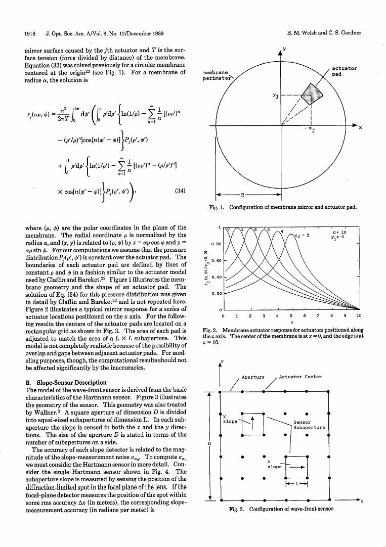
mirror surface caused by the jth actuator and T is the sur-face tension (force divided by distance) of the membrane.Equation (33) was solved previously for a circular membranecentered at the origin23 (see Fig. 1). For a membrane ofradius a, the solution is

rj(ap.) 2 T d0' (: p'dp' {ln(1/p) - n

-(p,/p)ncos[n(//'- )]}PI(p, 0)

+ Lp'dp' {ln(1/p') 1 [(p)n - (p/p1)n]n

n=1

X cos[n(,' -0 )]}PI(p 1)) (34)i1 a t m

Fig. 1. Configuration of membrane mirror and actuator pad.

where (p, p) are the polar coordinates in the plane of themembrane. The radial coordinate p is normalized by theradius a, and (x, y) is related to (p, 0) by x = ap cos 0 and y =ap sin 0. For our computations we assume that the pressuredistribution Pj(p', 0') is constant over the actuator pad. Theboundaries of each actuator pad are defined by lines ofconstant p and 0 in a fashion similar to the actuator modelused by Claflin and Bareket.2 2 Figure 1 illustrates the mem-brane geometry and the shape of an actuator pad. Thesolution of Eq. (34) for this pressure distribution was givenin detail by Claflin and Bareket2 2 and is not repeated here.Figure 2 illustrates a typical mirror response for a series ofactuator locations positioned on the x axis. For the follow-ing results the centers of the actuator pads are located on arectangular grid as shown in Fig. 3. The area of each pad isadjusted to match the area of a L X L subaperture. Thismodel is not.completely realistic because of the possibility ofoverlap and gaps between adjacent actuator pads. For mod-eling purposes, though, the computational results should notbe affected significantly by the inaccuracies.

B. Slope-Sensor DescriptionThe model of the wave-front sensor is derived from the basiccharacteristics of the Hartmann sensor. Figure 3 illustratesthe geometry of the sensor. This geometry was also treatedby Wallner.2 A square aperture of dimension D is dividedinto equal-sized subapertures of dimension L. In each sub-aperture the slope is sensed in both the x and the y direc-tions. The size of the aperture D is stated in terms of thenumber of subapertures on a side.

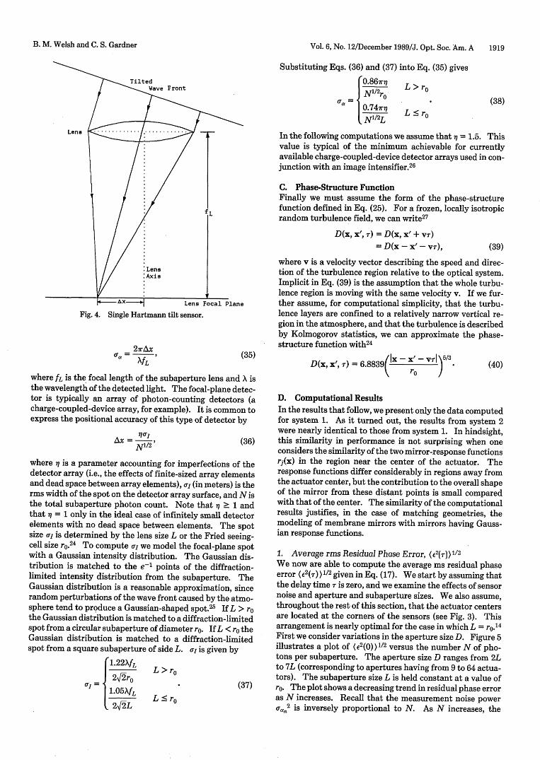
The accuracy of each slope detector is related to the mag-nitude of the slope-measurement noise oa,,n. To compute a,,1,we must consider the Hartmann sensor in more detail. Con-sider the single Hartmann sensor shown in Fig. 4. Thesubaperture slope is measured by sensing the position of thediffraetion-linlited spot ill the focal plane of the lens. If thefocal-plane detector measures the position of the spot withinsome rms accuracy Ax (in meters), the corresponding slope-measurement accuracy (in radians per meter) is

0. 80

0C; 0. 60

>i 0. 40

0. 20

00 1 2 3 4 5 6 7 9 10

x

Fig. 2. Membrane actuator response for actuators positioned alongthe x axis. The center of the membrane is at x = 0, and the edge is atX = 10.

y

Aperture/ Actuator Center

slope :SensorSubaperture

D~~~~~~~~

Fig. 3. Configuration of wave-front sensor.

y

x



Substituting Eqs. (36) and (37) into Eq. (35) gives

I.

'0.867r7q

Nl/2r .¢a 0747rq

12L

L > ro

(38)L • ro

Fig. 4. Single Hartmann tilt sensor.

27rAx0cr= -v

In the following computations we assume thatq = 1.5. Thisvalue is typical of the minimum achievable for currentlyavailable charge-coupled-device detector arrays used in con-junction with an image intensifier.26

C. Phase-Structure FunctionFinally we must assume the form of the phase-structurefunction defined in Eq. (25). For a frozen, locally isotropicrandom turbulence field, we can write27

D(x, x, T) = D(x, x' + VT)

where v is a velocity vector describing the speed and direc-tion of the turbulence region relative to the optical system.Implicit in Eq. (39) is the assumption that the whole turbu-lence region is moving with the same velocity v. If we fur-ther assume, for computational simplicity, that the turbu-lence layers are confined to a relatively narrow vertical re-gion in the atmosphere, and that the turbulence is describedby Kolmogorov statistics, we can approximate the phase-structure function with24

(35)

where fL is the focal length of the subaperture lens and X isthe wavelength of the detected light. The focal-plane detec-tor is typically an array of photon-counting detectors (acharge-coupled-device array, for example). It is common toexpress the positional accuracy of this type of detector by

AX 1/ (36)N 112

where 11 is a parameter accounting for imperfections of thedetector array (i.e., the effects of finite-sized array elementsand dead space between array elements), cr (in meters) is therms width of the spot on the detector array surface, and N isthe total subaperture photon count. Note that t 1 andthat = 1 only in the ideal case of infinitely small detectorelements with no dead space between elements. The spotsize a, is determined by the lens size L or the Fried seeing-cell size r. 24 To compute rI we model the focal-plane spotwith a Gaussian intensity distribution. The Gaussian dis-tribution is matched to the e points of the diffraction-limited intensity distribution from the subaperture. TheGaussian distribution is a reasonable approximation, sincerandom perturbations of the wave front caused by the atmo-sphere tend to produce a Gaussian-shaped spot.25 If L > rOthe Gaussian distribution is matched to a diffraction-limitedspot from a circular subaperture of diameter r. If L < r theGaussian distribution is matched to a diffraction-limitedspot from a square subaperture of side L. cr is given by

r(l.22AfL

1 2r L > ro

c 1 5XfL ()l22L L < ro

D(x, x', T) = 6 )8839 Ix - x'- vJ)5/3

D. Computational ResultsIn the results that follow, we present only the data computedfor system 1. As it turned out, the results from system 2were nearly identical to those from system 1. In hindsight,this similarity in performance is not surprising when oneconsiders the similarity of the two mirror-response functionsrj(x) in the region near the center of the actuator. Theresponse functions differ considerably in regions away fromthe actuator center, but the contribution to the overall shapeof the mirror from these distant points is small comparedwith that of the center. The similarity of the computationalresults justifies, in the case of matching geometries, themodeling of membrane mirrors with mirrors having Gauss-ian response functions.

1. Average rms Residual Phase Error, (E2(T))1/2We now are able to compute the average ms residual phaseerror (e 2(T))1 /2 given in Eq. (17). We start by assuming thatthe delay time T is zero, and we examine the effects of sensornoise and aperture and subaperture sizes. We also assume,throughout the rest of this section, that the actuator centersare located at the corners of the sensors (see Fig. 3). Thisarrangement is nearly optimal for the case in which L = ro.14First we consider variations in the aperture size D. Figure 5illustrates a plot of (e2(0))1/2 versus the number N of pho-tons per subaperture. The aperture size D ranges from 2Lto 7L (corresponding to apertures having from 9 to 64 actua-tors). The subaperture size L is held constant at a value ofro. The plot shows a decreasing trend in residual phase erroras N increases. Recall that the measurement noise powerOr,,1

2 is inversely proportional to N. As N increases, the

= D(x - x'- VT), (39)

(40)


1920 J. Opt: Soc. Am. A/Vol. 6, No. 12/December 1989

2.50 -

2 -

1.50

1

0.50

o 0 102 10

10 10 12 103

Photocounts/Subaperture. N

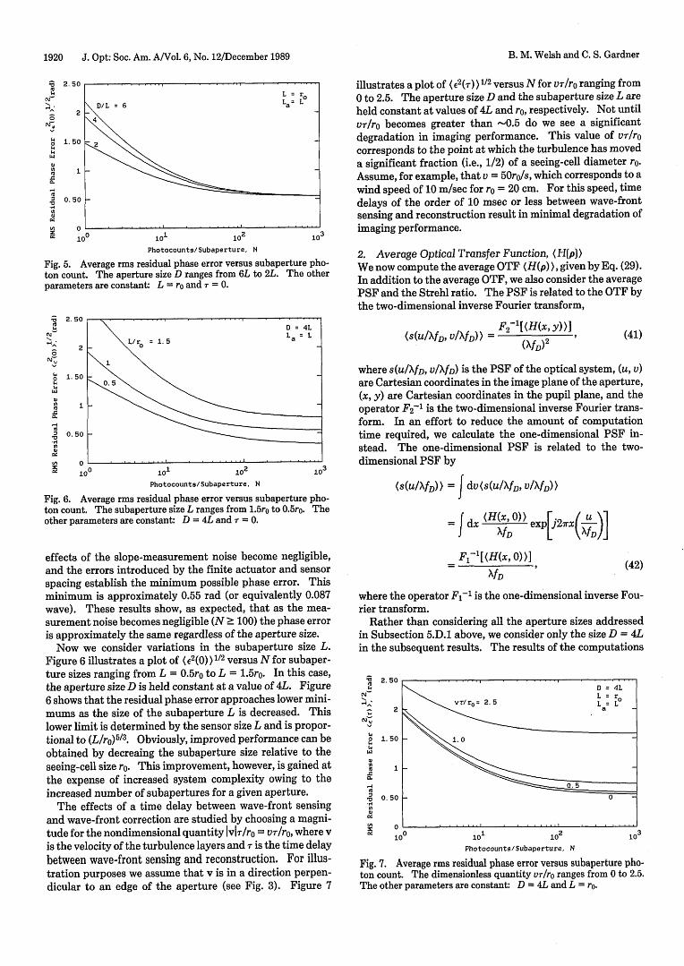
Fig. 5. Average rms residual phase error versus subaperture pho-ton count. The aperture size D ranges from 6L to 2L. The otherparameters are constant: L = ro and T = 0.

2. 50

2

1.50

1

0. 50

0 -100 10I 1o2 103

Photocounts/Subaperture. N

Fig. 6. Average rms residual phase error versus subaperture pho-ton count. The subaperture size L ranges from 1.5ro to 0.5ro. Theother parameters are constant: D = 4L and T = 0.

effects of the slope-measurement noise become negligible,and the errors introduced by the finite actuator and sensorspacing establish the minimum possible phase error. Thisminimum is approximately 0.55 rad (or equivalently 0.087wave). These results show, as expected, that as the mea-surement noise becomes negligible (N ' 100) the phase erroris approximately the same regardless of the aperture size.

Now we consider variations in the subaperture size L.Figure 6 illustrates a plot of (e2(0) ) 1/2 versus N for subaper-ture sizes ranging from L = 0.5ro to L = 1.5ro. In this case,the aperture size D is held constant at a value of 4L. Figure6 shows that the residual phase error approaches lower mini-mums as the size of the subaperture L is decreased. Thislower limit is determined by the sensor size L and is propor-tional to (L/ro) 513 . Obviously, improved performance can beobtained by decreaing the subaperture size relative to theseeing-cell size ro. This improvement, however, is gained atthe expense of increased system complexity owing to theincreased number of subapertures for a given aperture.

The effects of a time delay between wave-front sensingand wave-front correction are studied by choosing a magni-tude for the nondimensional quantity Ivl/ro = vrlro, where vis the velocity of the turbulence layers and T is the time delaybetween wave-front sensing and reconstruction. For illus-tration purposes we assume that v is in a direction perpen-dicular to an edge of the aperture (see Fig. 3). Figure 7

illustrates a plot of ( 2(r) ) 1/2 versus N for vr/ro ranging from0 to 2.5. The aperture size D and the subaperture size L areheld constant at values of 4L and ro, respectively. Not untilvTrro becomes greater than -0.5 do we see a significantdegradation in imaging performance. This value of vT/rocorresponds to the point at which the turbulence has moveda significant fraction (i.e., 1/2) of a seeing-cell diameter r.Assume, for example, that v = 50ro/s, which corresponds to awind speed of 10 m/sec for ro = 20 cm. For this speed, timedelays of the order of 10 msec or less between wave-frontsensing and reconstruction result in minimal degradation ofimaging performance.

2. Average Optical Transfer Function, (H(p))We now compute the average OTF (H(p)), given by Eq. (29).In addition to the average OTF, we also consider the averagePSF and the Strehl ratio. The PSF is related to the OTF bythe two-dimensional inverse Fourier transform,

F2'[(H(x, y))](suINf, VIXfD)) = (XfD)2 (41)

where s(UD, vufD) is the PSF of the optical system, (u, v)are Cartesian coordinates in the image plane of the aperture,(x, y) are Cartesian coordinates in the pupil plane, and theoperator F2-1 is the two-dimensional inverse Fourier trans-form. In an effort to reduce the amount of computationtime required, we calculate the one-dimensional PSF in-stead. The one-dimensional PSF is related to the two-dimensional PSF by

(S(UIfD) ) = J dv(s(uI/fD, VIXJD))

= J dx (HXf)) exp[ 2rx(j-)]

Fl-'[(H(x, 0))]

XfD(42)

where the operator Fr-1 is the one-dimensional inverse Fou-rier transform.

Rather than considering all the aperture sizes addressedin Subsection 5.D.1 above, we consider only the size D = 4Lin the subsequent results. The results of the computations

NW

P

W

1.

Ia'

2. 50

2

1.50

o

0. 50

0 100 10I 102

Photocounts/Subaperture, N

Fig. 7. Average rms residual phase error versus subaperture pho-ton count. The dimensionless quantity vr/ro ranges from 0 to 2.5.The other parameters are constant: D = 4L and L = ro.


'a;:GW

1111�a

clj-.

0WW

Inla.C

'a1-40

'AIDM

'aGW

cm

a

1.1

0la.C'a

'A0W

"I


0. 80

W

C1

0

11

0. 60

0. 40

0 1 10 0.20 0.40 0.60 0.80 1

p/D

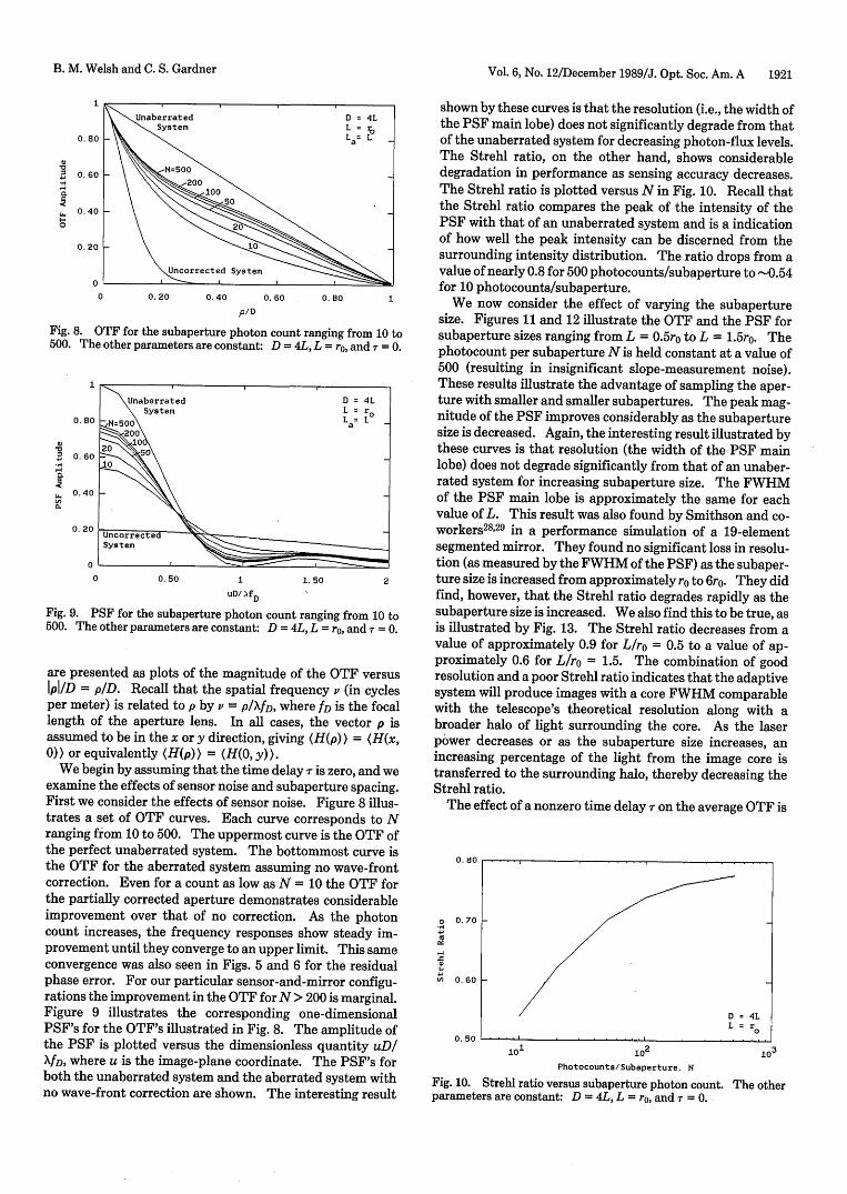
Fig. 8. OTF for the subaperture photon count ranging from 10 to500. The other parameters are constant: D = 4L, L = r, and T = 0.

0. 80

B;

,§1-

VW

0. 60

0.40

0. 20

01L

0 0.50 1 1.50uD/ )fD

Fig. 9. PSF for the subaperture photon count ranging from 10 to500. The other parameters are constant: D = 4L, L = r, and r = 0.

are presented as plots of the magnitude of the OTF versusJphID = pD. Recall that the spatial frequency v (in cyclesper meter) is related to p by v = p/Xfn, where fD is the focallength of the aperture lens. In all cases, the vector p isassumed to be in the x or y direction, giving (H(p)) = (H(x,0)) or equivalently (H(p)) = (H(O, y)).

We begin by assuming that the time delay r is zero, and weexamine the effects of sensor noise and subaperture spacing.First we consider the effects of sensor noise. Figure 8 illus-trates a set of OTF curves. Each curve corresponds to Nranging from 10 to 500. The uppermost curve is the OTF ofthe perfect unaberrated system. The bottommost curve isthe OTF for the aberrated system assuming no wave-frontcorrection. Even for a count as low as N = 10 the OTF forthe partially corrected aperture demonstrates considerableimprovement over that of no correction. As the photoncount increases, the frequency responses show steady im-provement until they converge to an upper limit. This sameconvergence was also seen in Figs. 5 and 6 for the residualphase error. For our particular sensor-and-mirror configu-rations the improvement in the OTF for N > 200 is marginal.Figure 9 illustrates the corresponding one-dimensionalPSF's for the OTF's illustrated in Fig. 8. The amplitude ofthe PSF is plotted versus the dimensionless quantity uDIXfD, where u is the image-plane coordinate. The PSF's forboth the unaberrated system and the aberrated system withno wave-front correction are shown. The interesting result

shown by these curves is that the resolution (i.e., the width ofthe PSF main lobe) does not significantly degrade from thatof the unaberrated system for decreasing photon-flux levels.The Strehl ratio, on the other hand, shows considerabledegradation in performance as sensing accuracy decreases.The Strehl ratio is plotted versus N in Fig. 10. Recall thatthe Strehl ratio compares the peak of the intensity of thePSF with that of an unaberrated system and is a indicationof how well the peak intensity can be discerned from thesurrounding intensity distribution. The ratio drops from avalue of nearly 0.8 for 500 photocounts/subaperture to -0.54for 10 photocounts/subaperture.

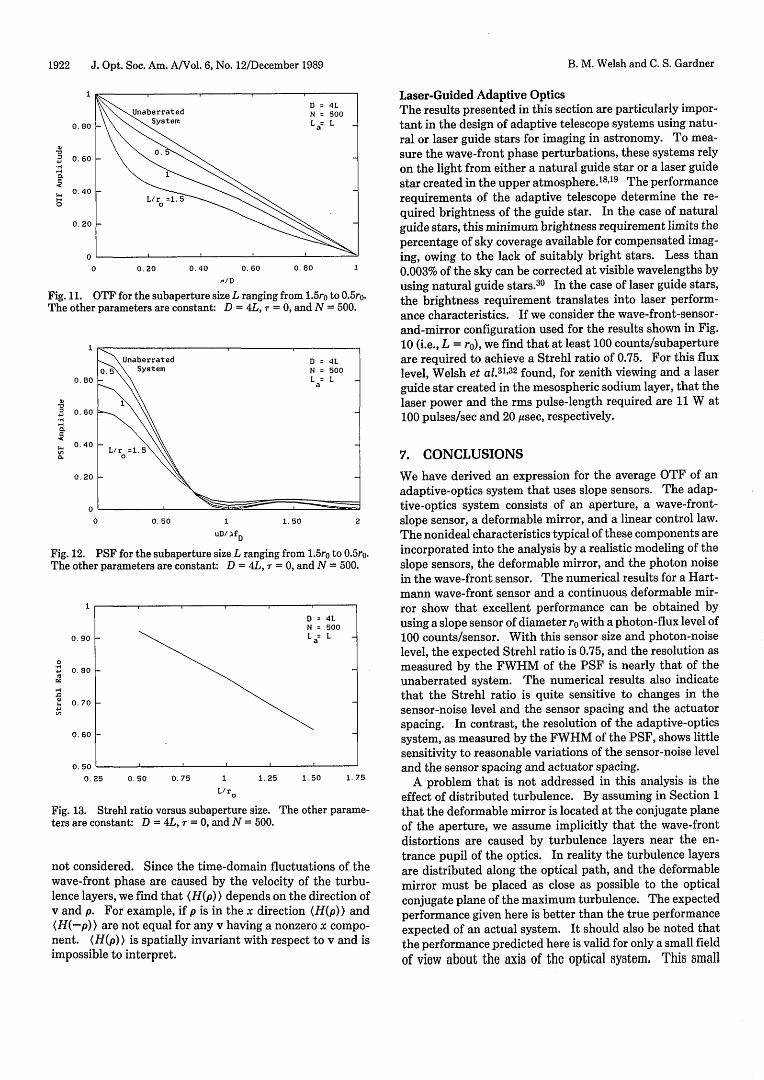
We now consider the effect of varying the subaperturesize. Figures 11 and 12 illustrate the OTF and the PSF forsubaperture sizes ranging from L = 0.5ro to L = 1.5rO. Thephotocount per subaperture N is held constant at a value of500 (resulting in insignificant slope-measurement noise).These results illustrate the advantage of sampling the aper-ture with smaller and smaller subapertures. The peak mag-nitude of the PSF improves considerably as the subaperturesize is decreased. Again, the interesting result illustrated bythese curves is that resolution (the width of the PSF mainlobe) does not degrade significantly from that of an unaber-rated system for increasing subaperture size. The FWHMof the PSF main lobe is approximately the same for eachvalue of L. This result was also found by Smithson and co-workers28' 2 9 in a performance simulation of a 19-elementsegmented mirror. They found no significant loss in resolu-tion (as measured by the FWHM of the PSF) as the subaper-ture size is increased from approximately r to 6ro. They didfind, however, that the Strehl ratio degrades rapidly as thesubaperture size is increased. We also find this to be true, asis illustrated by Fig. 13. The Strehl ratio decreases from avalue of approximately 0.9 for L/ro = 0.5 to a value of ap-proximately 0.6 for L/ro = 1.5. The combination of goodresolution and a poor Strehl ratio indicates that the adaptivesystem will produce images with a core FWHM comparablewith the telescope's theoretical resolution along with abroader halo of light surrounding the core. As the laserpower decreases or as the subaperture size increases, anincreasing percentage of the light from the image core istransferred to the surrounding halo, thereby decreasing theStrehl ratio.

The effect of a nonzero time delayTr on the average OTF is

0. 8O

0

a1

4-

0. 70

0. 60

0. 50

10 102 103Photocounts/Subaperture, N

Fig. 10. Strehl ratio versus subaperture photon count. The otherparameters are constant: D = 4L, L = r, and = 0.



0. 80

0

4-,

To

0. 60

0. 40

0. 20,, 0:! 1

0 0. 20 0. 40 0. 60 0. 80 1

,/D

Fig. 11. OTF for the subaperture size L ranging from 1.5ro to 0.5ro.The other parameters are constant: D = 4L, X = 0, and N = 500.

0. 80

S41-H`4c'

11

Q.

0. 60

0. 40

0. 20

01L

0 0.50 1 1.50uD/ fD

Fig. 12. PSF for the subaperture size L ranging from 1.5ro to 0.5ro.The other parameters are constant: D = 4L, = 0, and N = 500.

0. 90

0

41

.,

0. 80

0. 70

0. 60

0. 50 _0.25 0.50 0.75 1 1.25 1.50 1.75

L/r

Fig. 13. Strehl ratio versus subaperture size. The other parame-ters are constant: D = 4L, r = 0, and N = 500.

not considered. Since the time-domain fluctuations of thewave-front phase are caused by the velocity of the turbu-lence layers, we find that (H(p)) depends on the direction ofv and p. For example, if p is in the x direction (H(p)) and(H(-p)) are not equal for any v having a nonzero x compo-nent. (H(p)) is spatially invariant with respect to v and isimpossible to interpret.

Laser-Guided Adaptive OpticsThe results presented in this section are particularly impor-tant in the design of adaptive telescope systems using natu-ral or laser guide stars for imaging in astronomy. To mea-sure the wave-front phase perturbations, these systems relyon the light from either a natural guide star or a laser guidestar created in the upper atmosphere.18 19 The performancerequirements of the adaptive telescope determine the re-quired brightness of the guide star. In the case of naturalguide stars, this minimum brightness requirement limits thepercentage of sky coverage available for compensated imag-ing, owing to the lack of suitably bright stars. Less than0.003% of the sky can be corrected at visible wavelengths byusing natural guide stars.3 0 In the case of laser guide stars,the brightness requirement translates into laser perform-ance characteristics. If we consider the wave-front-sensor-and-mirror configuration used for the results shown in Fig.10 (i.e., L = ro), we find that at least 100 counts/subapertureare required to achieve a Strehl ratio of 0.75. For this fluxlevel, Welsh et al.31' 32 found, for zenith viewing and a laserguide star created in the mesospheric sodium layer, that thelaser power and the rms pulse-length required are 11 W at100 pulses/sec and 20 ,sec, respectively.

7. CONCLUSIONS

We have derived an expression for the average OTF of anadaptive-optics system that uses slope sensors. The adap-tive-optics system consists of an aperture, a wave-front-slope sensor, a deformable mirror, and a linear control law.The nonideal characteristics typical of these components areincorporated into the analysis by a realistic modeling of theslope sensors, the deformable mirror, and the photon noisein the wave-front sensor. The numerical results for a Hart-mann wave-front sensor and a continuous deformable mir-ror show that excellent performance can be obtained byusing a slope sensor of diameter ro with a photon-flux level of100 counts/sensor. With this sensor size and photon-noiselevel, the expected Strehl ratio is 0.75, and the resolution asmeasured by the FWHM of the PSF is nearly that of theunaberrated system. The numerical results also indicatethat the Strehl ratio is quite sensitive to changes in thesensor-noise level and the sensor spacing and the actuatorspacing. In contrast, the resolution of the adaptive-opticssystem, as measured by the FWHM of the PSF, shows littlesensitivity to reasonable variations of the sensor-noise leveland the sensor spacing and actuator spacing.

A problem that is not addressed in this analysis is theeffect of distributed turbulence. By assuming in Section 1that the deformable mirror is located at the conjugate planeof the aperture, we assume implicitly that the wave-frontdistortions are caused by turbulence layers near the en-trance pupil of the optics. In reality the turbulence layersare distributed along the optical path, and the deformablemirror must be placed as close as possible to the opticalconjugate plane of the maximum turbulence. The expectedperformance given here is better than the true performanceexpected of an actual system. It should also be noted thatthe performance predicted here is valid for only a small fieldof view about the axis of the optical system. This small



angular region is specified by the isoplanatic angle.33 Again,this restriction of the applicability of the analysis is causedby the distribution of the turbulence along the optical path..

ACKNOWLEDGMENTS

This study was supported in part by National Science Foun-dation grants ATM 86-10142 and ATM 88-11771. The au-thors gratefully acknowledge the many helpful discussionswith Laird A. Thompson.

REFERENCES

1. J. W. Hardy, "Active optics: a new technology for the control oflight," Proc. IEEE 66, 651-697 (1978).

2. E. P. Wallner, "Optimal wave-front correction using slope mea-surements," J. Opt. Soc. Am. 73, 1771-1776 (1983).

3. E. P. Wallner, "Comparison of wave front sensor configurationsusing optimal reconstruction and correction," in WavefrontSensing, N. Bareket and C. L. Koliopoulos, eds., Proc. Soc.Photo-Opt. Instrum. Eng. 351, 42-53 (1982).

4. D. L. Fried, "Least-square fitting a wave-front distortion esti-mate to an array of phase-difference measurements," J. Opt.Soc. Am. 67, 370-375 (1977).

5. R. H. Hudgin, "Wave-front reconstruction for compensatedimaging," J. Opt. Soc. Am. 67, 375-377 (1977).

6. R. J. Noll, "Phase estimates from slope-type wave-front sen-sors," J. Opt. Soc. Am. 68, 139-140 (1978).

7. J. Herrmann, "Least-squares wave front errors of minimumnorm," J. Opt. Soc. Am. 70, 28-35 (1980).

8. W. H. Southwell, "Wave-front estimation from wave-front slopemeasurements," J. Opt. Soc. Am. 70, 998-1005 (1980).

9. K. Freischlad and C. Koliopoulos, "Wave front reconstructionfrom noisy slope or difference data using the discrete Fouriertransform," in Adaptive Optics, J. E. Ludman, ed., Proc. Soc.Photo-Opt. Instrum. Eng. 551, 74-80 (1985).

10. J. Hermann, "Cross coupling and aliasing in modal wave-frontestimation," J. Opt. Soc. Am. 71, 989-992 (1981).

11. R. Cubalchini, "Modal wave-front estimation from phase deriv-ative measurements," J. Opt. Soc. Am. 69, 972-977 (1979).

12. R. H. Hudgin, "Optimal wave-front estimation," J. Opt. Soc.Am. 67, 378-382 (1977).

13. R. Hudgin, "Wave-front compensation error due to finite cor-rector-element size," J. Opt. Soc. Am. 67, 393-395 (1977).

14. J. P. Gaffard and C. Boyer, "Adaptive optics for optimization ofimage resolution," Appl. Opt. 26, 3772-3777 (1987).

15. D. P. Greenwood, "Mutual coherence function of a wave frontcorrected by zonal adaptive optics," J. Opt. Soc. Am. 69, 549-554 (1979).

16. J. Y. Wang, "Optical resolution through a turbulent medium

with adaptive phase compensations," J. Opt. Soc. Am. 67, 383-390 (1977).

17. J. Y. Wang and J. K. Markey, "Modal compensation of atmo-spheric turbulence phase distortion," J. Opt. Soc. Am. 68, 78-87(1978).

18. L. A. Thompson and C. S. Gardner, "Experiments on laser guidestars at Mauna Kea Observatory for adaptive imaging in astron-omy," Nature 328, 229-231 (1987).

19. C. S. Gardner, B. M. Welsh, and L. A. Thompson, "Design andperformance analysis of adaptive optical telescopes using laserguide stars," submitted to Proc. IEEE.

20. J. W. Goodman, Statistical Optics (Wiley, New York, 1985), p.364.

21. A. T. Young, "Seeing: its cause and cure," Astrophys. J. 189,587-604 (1974).

22. E. S. Claflin and N. Baraket, "Configuring an electrostaticmembrane mirror by least-squares fitting with analytically de-rived influence functions," J. Opt. Soc. Am. A 3, 1833-1839(1986).

23. P. M. Morse and H. Fesbback, Methods of Theoretical Physics,Part II (McGraw-Hill, New York, 1953), p. 1191.

24. D. L. Fried, "Optical resolution through a randomly inhomo-geneous medium for very long and very short exposures," J.Opt. Soc. Am. 56, 1372-1379 (1966).

25. K. A. Winick, "Cramnr-Rao lower bounds on the performanceof charge-coupled-device optical position estimators," J. Opt.Soc. Am. A 3, 1809-1815 (1986).

26. T. J. Kane, B. M. Welsh, C. S. Gardner, and L. A. Thompson,"Wave front detector optimization for laser guided adaptivetelescopes," in Active Telescope Systems, F. Roddier, ed., Proc.Soc. Photo-Opt. Instrum. Eng. 1114, 160-171 (1989).

27. V. I. Tatarski, The Effects of the Turbulent Atmosphere onWave Propagation (National Technical Information Service,Springfield, Va., 1971), p. 35.

28. R. C. Smithson, Michal L. Peri, and Robert S. Benson, "Quanti-tative simulation of image correction for astronomy with a seg-mented active mirror," Appl. Opt. 27, 1615-1620 (1988).

29. R. C. Smithson and Michal L. Peri, "Partial correction of astro-nomical images with active mirrors," J. Opt. Soc. Am. A 6, 92-97 (1989).

30. J. M. Beckers, F. J. Roddier, P. R. Eisenhardt, L. E. Goad, andK.-L. Shu, "National Optical Astronomy observatories (NOAO)Infrared Adaptive Optics Program I: general description," inAdvanced Technology Optical Telescopes III, L. D. Barr, ed.,Proc. Soc. Photo-Opt. Instrum. Eng. 628, 290-297 (1986).

31. B. M. Welsh and C. S. Gardner, "Nonlinear resonant absorp-tion effects on the design of resonance fluorescence lidars andlaser guide stars," Appl. Opt. 28, 4141-4153 (1989).

32. B. M. Welsh, C. S. Gardner, and L. A. Thompson, "Effects ofnonlinear resonant absorption on sodium laser guide stars," inActive Telescope Systems, F. Roddier, ed., Proc. Soc. Photo-Opt. Instrum. Eng. 1114, 203-214 (1989).

33. D. L. Fried, "Anisoplanatism in adaptive optics," J. Opt. Soc.Am. 72, 52-61 (1982).


performance analysis of adaptive-optics systems using laser guide stars and slope sensors

Documents