University of South FloridaScholar Commons

Graduate Theses and Dissertations Graduate School

2009

Performance analysis of a binary-tree-basedalgorithm for computing Spatial DistanceHistogramsSadhana Sharma LuetelUniversity of South Florida

Follow this and additional works at: http://scholarcommons.usf.edu/etd

Part of the American Studies Commons

This Thesis is brought to you for free and open access by the Graduate School at Scholar Commons. It has been accepted for inclusion in GraduateTheses and Dissertations by an authorized administrator of Scholar Commons. For more information, please contact scholarcommons@usf.edu.

Scholar Commons CitationSharma Luetel, Sadhana, "Performance analysis of a binary-tree-based algorithm for computing Spatial Distance Histograms" (2009).Graduate Theses and Dissertations.http://scholarcommons.usf.edu/etd/16

Performance Analysis of a Binary-Tree-Based Algorithm for Computing Spatial Distance

Histograms

by

Sadhana Sharma Luetel

A thesis submitted in partial fulfillmentof the requirements for the degree of

Master of Science in Computer ScienceDepartment of Computer Science and Engineering

College of EngineeringUniversity of South Florida

Major Professor: Yicheng Tu, Ph.D.Rafael Perez, Ph.D.

Rahul Tripathi, Ph.D.Sagar Pandit, Ph.D.

Date of Approval:October 30, 2009

Keywords: Spatial Distance Histogram, Particle Distance Histogram, Quad-tree, Binary tree,Uniformity

c© Copyright 2009, Sadhana Sharma Luetel

ACKNOWLEDGEMENTS

First and foremost I would like to express my sincere gratitude to my M.S. advisor Dr. Yi-

Cheng Tu for providing me the wonderful opportunity for continuing my education. I always

respect him for providing me the confidence and support to begin the thesis in the area of my

interest of database management systems.

I would like to express heartfelt gratitude towards Dr. Rafael Perez who gave me the

opportunity to work as a “Graduate Assistant” for the “College of Engineering”.

I would like to extend my appreciation to the committee members for their support and

encouragement.

I would like to express my loving thanks to my husband Mr. Prakash Luetel for his regular

support, encouragement and motivation throughout my thesis.

Lastly, and most importantly, I wish to thank my parents, Mr. Lakshmi Dhar Guragain

and Mrs. Sapana Pokharel Guragain for their unconditional love and support throughout my

life. To them, I dedicate this thesis.

TABLE OF CONTENTS

LIST OF TABLES ii

LIST OF FIGURES iii

ABSTRACT iv

CHAPTER 1 INTRODUCTION 1

CHAPTER 2 OVERVIEW OF PRIOR WORK 32.1 Introduction to Quad-tree 42.2 Spatial Distance Histogram 52.3 Implementation of Density Maps 62.4 The DM-SDH Algorithm 62.5 Time Complexity 82.6 Discussion and Conclusion of Prior Work 9

CHAPTER 3 BINARY TREE STRUCTURE 103.1 Organization of Tree Structure 113.2 Analysis of the Algorithm 133.3 Experimental Results 21

CHAPTER 4 INSPECTING UNIFORM REGIONS HOPING TO IMPROVE THEPERFORMANCE 25

4.1 The Goodness of Fit Test 254.2 R - for Statistical Computing 27

CHAPTER 5 CONCLUSION AND FUTURE ENHANCEMENTS 305.1 Conclusion 305.2 Future Enhancements 30

REFERENCES 32

i

LIST OF TABLES

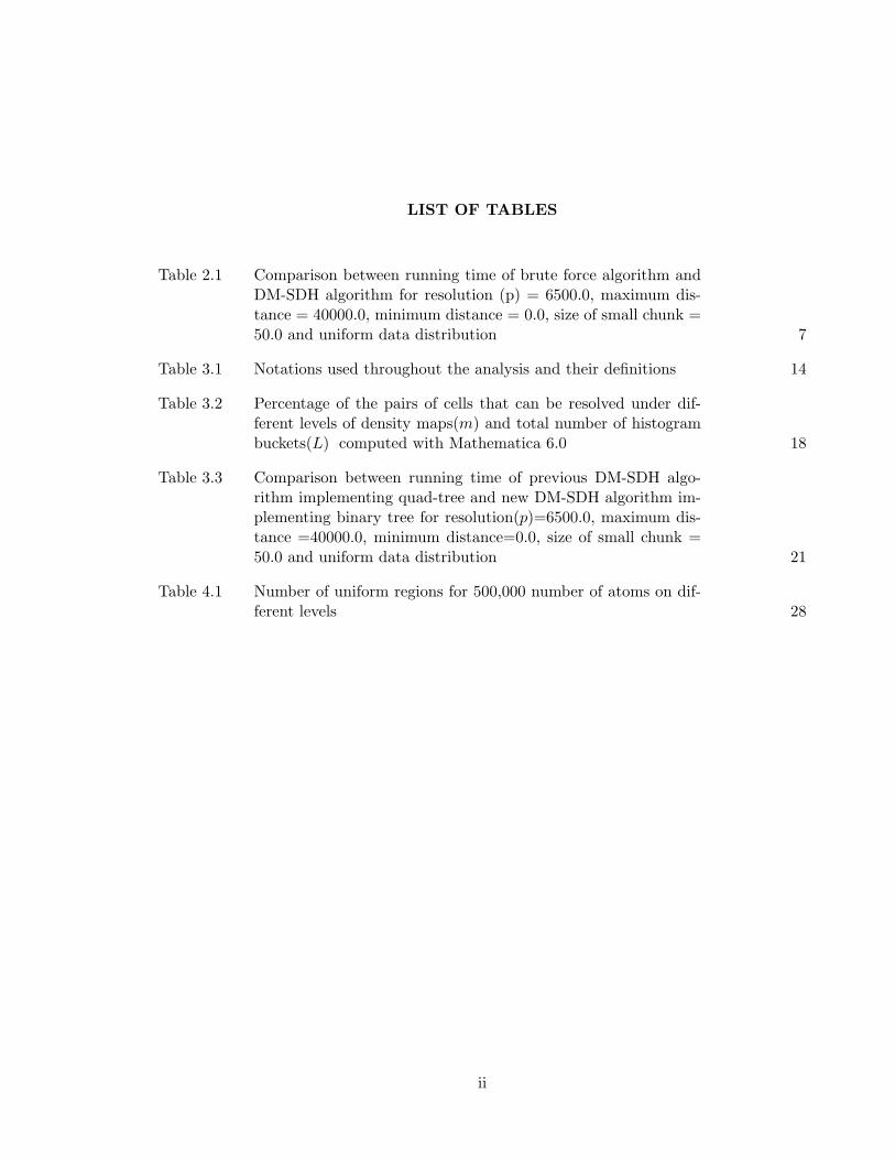
Table 2.1 Comparison between running time of brute force algorithm andDM-SDH algorithm for resolution (p) = 6500.0, maximum dis-tance = 40000.0, minimum distance = 0.0, size of small chunk =50.0 and uniform data distribution 7

Table 3.1 Notations used throughout the analysis and their definitions 14

Table 3.2 Percentage of the pairs of cells that can be resolved under dif-ferent levels of density maps(m) and total number of histogrambuckets(L) computed with Mathematica 6.0 18

Table 3.3 Comparison between running time of previous DM-SDH algo-rithm implementing quad-tree and new DM-SDH algorithm im-plementing binary tree for resolution(p)=6500.0, maximum dis-tance =40000.0, minimum distance=0.0, size of small chunk =50.0 and uniform data distribution 21

Table 4.1 Number of uniform regions for 500,000 number of atoms on dif-ferent levels 28

ii

LIST OF FIGURES

Figure 2.1 Density maps with different resolutions for same dataset 4

Figure 2.2 Minimum and maximum distance between cells A-B and A-Cwhere the dotted lines represent maximum distances and solidlines represent minimum distances 7

Figure 2.3 ResolveTwoCells() function 8

Figure 2.4 Tree structure of the density map 8

Figure 3.1 A general binary tree 11

Figure 3.2 Partitions of nodes (a) shows parent node, (a) is partitioned as(b) in second level and as (c) in third level 11

Figure 3.3 Density maps implemented via a binary tree approach 12

Figure 3.4 Binary tree to organize the density map 13

Figure 3.5 BuildBinaryTree() algorithm 22

Figure 3.6 A is the cell with bucket width p, bucket 1 is the region boundedby curves C1 to C8 and bucket 2 is the region bounded by curvesD1 to D8 [1] 23

Figure 3.7 Conceptual tree structure with three density maps where thehidden line signifies the intermediate density map 23

Figure 3.8 Time taken by quad tree implemented algorithm (qPDH) andbinary tree implemented algorithm (bPDH) vs number of nodes(in x axis) 24

Figure 3.9 Ratio of the time taken by previous algorithm and new algorithm(in y axis) vs number of nodes (in x axis) 24

Figure 4.1 If B is uniform, the children nodes of B are also uniform 26

Figure 4.2 If B is uniform, the cells in B are also uniform 26

Figure 4.3 FindingUniformRegions() algorithm 27

Figure 4.4 Chi-Square table 28

iii

PERFORMANCE ANALYSIS OF A BINARY-TREE-BASED ALGORITHMFOR COMPUTING SPATIAL DISTANCE HISTOGRAMS

Sadhana Sharma Luetel

ABSTRACT

The environment is made up of composition of small particles. Hence, particle simulation

is an important tool in many scientific and engineering research fields to simulate the real life

processes of the environment. Because of the enormous amount of data in such simulations,

data management, storage and processing are very challenging tasks. Spatial Distance His-

togram (SDH) is one of the most popular queries being used in this field. In this thesis, we

are interested in investigating the performance of improvement of an existing algorithm for

computing SDH. The algorithm already being used is using a conceptual data structure called

density map which is implemented via a quad tree index. An algorithm having density maps

implemented via binary tree is proposed in this thesis. After carrying out many experiments

and analysis of the data, we figure out that although the binary tree approach seems efficient

in earlier stage, it is same as the quad tree approach in terms of time complexity. However,

it provides an improvement in computing time by a constant factor for some data inputs.

The second part of this thesis is dedicated to an approach that can potentially reduce the

computational time to a great extent by taking advantage of regions where data points are

uniformly distributed.

iv

CHAPTER 1

INTRODUCTION

Computer simulation allows the scientists to determine the features of the system and

visualize it virtually before the system is actually built. It results the efficient and effective

construction of the system. Almost all the scientific fields are using the goodness of com-

puter simulation in today’s world. Scientific particle simulations are getting more popular in

scientific and engineering fields such as material science, astro-physics, biomedical sciences,

chemistry and so on. They are demanding huge data storage systems imposing great chal-

lenge in analyzing, storing and processing the data.[4] Here, we deal with the techniques and

algorithms which are very important in the analysis of the particle simulation data.

A Histogram is a data structure maintained by a Database Management System (DBMS)

to approximate data distribution. The data distribution can be approximated by assigning

the data values in particular the sub-range of the value called buckets. Histograms can be of

many types and are used as query optimizer in many database systems.

Particle Simulation, a subset of Computer Simulation, treats the basic entities of large

systems as ”classical entities” that interact to one another via empirical forces. Data gener-

ated by particle simulations require huge database systems and query processing due to its

large volume of data. In such case of huge data set, we can implement the concept of Spatial

Distance histogram (SDH), which is considered as a fundamental tool in validation and anal-

ysis of such data. SDH is a type of query that maintains the histogram of distances among

the pairs of particles within the system. It is the direct estimation of radial distribution func-

tion (RDH), which is a continuous statistical distribution function that describes relationship

between density of surrounding matter and function of distance from a particular point. [3]

1

Chapter 2 describes the overview of previous work done to compute the distance histogram.

It presents the density map data-structure which is implemented by using quad-tree index and

analyzes the algorithm.

Chapter 3 presents the idea of binary tree implemented SDH concept. It presents the

density map data structure implemented using binary tree. It presents the experimental results

and observations being made for different datasets. This chapter also compares the results

obtained by quad tree implementation of density maps and the binary tree implementation

of density maps.

Chapter 4 presents the novel idea of implementing uniformity test in the data so as to

reduce the computing time. It describes the Chi-square goodness of fit test which is being used

to figure out the uniformity among the codes and describes how the test can be implemented

in our system.

Chapter 5 presents the conclusion and future enhancement of this thesis.

2

CHAPTER 2

OVERVIEW OF PRIOR WORK

Usually the volume of scientific data is so large that it becomes a challenge to store and

retrieve such data using current DBMS systems. Particle simulation is an example of such

scientific data in which basic components of large systems are treated as the classical entities

that interact for certain duration under postulated empirical forces. [1]

In case of large biomedical simulation systems, molecules are treated as the classical en-

tities. The molecules in such systems interact with each other for certain duration under

some force. Similarly, in case of astrological simulation system, particles all over the universe

are treated as the classical entities. And, the particles interact with one another for certain

duration under postulated empirical forces.

Huge space is required to store the results obtained by such particle simulation. For

example, a molecular simulation of the cell’s protein-making structure created by researchers

at Los Alamos National Laboratory simulates 2.64 million atoms. Although, the configurations

of particle simulation tend to store information about their types, velocities and coordinates,

scientists are mainly focused on the coordinates only. SDH keeps a histogram of the distances

of all pairs of the particles in the particle simulation system. If brute force method of SDH

os implemented, the algorithm requires O (N2) computations for N number of particles. On

the other hand, we can reduce the complexity to Θ(N3/2) if we implement a conceptual data

structure called density map in SDH algorithm as described in the prior work of this thesis

[1].

In [1], the density map is defined as a 2D grid that contains squares of equal size. Every

cell in the grid represents the simulated space and contains the number of particles located in

that space and the four coordinates of the cell. To process SDH, a series of density maps are

built. Each cell in the density map is divided into four disjoint cells in the next density map

3

Figure 2.1 Density maps with different resolutions for same dataset

as shown in figure 2.1 because the density map organized by connecting all the cells using

point-region (PR) quad tree approach. Each level in the quad-tree, becomes one resolution of

the density map.

2.1 Introduction to Quad-tree

As indicated by its name, quad tree is a tree structure which repeatedly divides the space

into quadrants. It is an example of space-partitioning trees. Quad-tree is used to describe

a class of hierarchical data structures whose common property is that they are based on the

principle of recursive decomposition of space. [2] Quad-trees are classified to different classes

depending upon the data they represent. The major sub-classes of quad-tree are:

• Point quad-tree

• Region quad-tree

• Edge quad-tree

Point quad-tree is very much similar to binary tree but it represents two dimensional point

data. It is implemented as a multi-dimensional generalization of a binary tree. Each node

had four children represented as NW(North-West), NE(North-East), SW(South-West) and

SE(South-East). All the children nodes contain point ( in x and y coordinates) and value of

that point.

4

Region quad-tree (also known as trie) is a branching structure which branches the region

into four equal quadrants. Each node in the tree has either exactly four children or no children

at all.

Edge quad-tree is used to represent the edges or lines rather than the points.

Regardless of the types, all quad trees partition the space into cells, and the tree follows

the spatial decomposition of the quad-tree.

In the DM-SDH algorithm, we implement the concept of PR(Point-Region) quad tree to

organize the density map. PR quad-tree adapts region quad tree to point data. It is pretty

much similar to region quad-tree but the difference is that unlike in region quad-tree, in PR

quad-trees, leaf nodes can be either empty or containing data.

2.2 Spatial Distance Histogram

While analyzing and researching on particle simulation data, spatial distance histogram

(SDH) is used as a basic tool. It is a direct estimation of a continuous statistical distribution

function known as “Radial Distribution Function” (RDF)[1]. RDF basically gives the proba-

bility of finding a particle in distance r of another particle. RDF can be viewed as normalized

SDH. RDF can be defined mathematically as:

g(r) =N(r)

4Πr2δrρ

where N(r) is the total number of atoms in space between r and r + δr around any particle

and ρ is the average density of all the particles in the system

RDF is very much important in thermodynamics and using this function, we can compute

the thermodynamic quantities of the system like pressure and energy.

SDH techniques are not yet used be the commercial database systems. In SDH Problem,

we have to calculate the distance between all given points and put them in a histogram bucket.

In this thesis, the width of all the histogram buckets are always the same, denoted by p.

5

2.3 Implementation of Density Maps

Density map is a conceptual data structure, used to calculate the point-to-point distances

on less time. For two dimensional data, it is a 2-D grid that divides the space into squares and

rectangles. While implementing quad tree structure, the grid divides the space into squares

and while implementing binary tree, the space is divided into rectangular spaces.

Each node of the key holds (p-count, x1, x2, y1, y2, child, p-list, next) where p-count is

the total number of atoms held by the node, x1, x2, y1, y2 define the bound of the square,

child points to the leftmost child of the node (so that child is -1 for the nodes at the leaf

level), p-list contains the data stored by the tree and next chains the nodes at the same level

together.

While building the tree, it is made sure that the space represented by every node is a

square first. Then, on change of each level, the space is partitioned in two dimensions to

get four more squares as depicted in figure 2.1. The density map shown in figure 2.1 can be

represented by a tree structure as shown in the figure 2.4.

In figure 2.4 DM3 has the highest resolution because it is at the lowest level (above the

leaf level), so, all the nodes of DM3 are connected to the data of the particles.

2.4 The DM-SDH Algorithm

Resolving two cells is the most important part of this process. Two of the cells in the same

density map are known as resolvable cells if the minimum and maximum distances between the

cells fall in the same histogram bucket. While determining whether the cells are resolvable or

not, any of the two cells of same density map are taken and minimum and maximum distances

between those two cells are calculated as shown in figure 2.2. If those distances fall into the

same histogram bucket, the two cells are resolvable into that bucket. If those distances do not

fall into a same histogram bucket, they do not resolve on the current density map and the

control is moved to the next level of the tree (or high resolution of the density map) and same

thing is repeated again. In this way, considering the number of atoms in the density map cells

to process multiple point-to-point distances at once, significantly improves the performance

6

Figure 2.2 Minimum and maximum distance between cells A-B and A-C where the dottedlines represent maximum distances and solid lines represent minimum distances

Table 2.1 Comparison between running time of brute force algorithm and DM-SDH algorithmfor resolution (p) = 6500.0, maximum distance = 40000.0, minimum distance = 0.0, size ofsmall chunk = 50.0 and uniform data distribution

No. of Atoms Brute-Force Algorithm DM-SDH Algorithm

50 0.000089 0.000135

500 0.008975 0.00504

5000 0.834 0.202

50000 82.5 5.9

100000 339.45 17.807

over the brute-force approach. The algorithm implemented for resolving two cells is as shown

in algorithm 2.3 [1].

In this tree, Minimum Bounding Rectangle (MBR) formed by the data particles contained

in a particular node is also being stored. MBR is being used to compute the minimum and

maximum point-to-point distances. The use of MBR in this algorithm makes more cells

resolvable at each level.

While building the tree, series of density maps is created starting from the zeroth level of

the tree, which has a single node map that covers whole space and has least resolution among

all density maps. The total level of density maps as shown in [1] is

H = log2d [N/β] + 1

where 2d is the degree of tree nodes ( 4 for 2-dimensional data), N is the total number of

atoms and β is the average number of particles in every node. In this algorithm, β is set to

be slightly greater than 4.

7

Input: Say A and B are the two input cells.if A and B are resolvable then

Add nA × nB to the corresponding bucket (Where nA and nB are the total numberof particles contained by A and B respectively)

endelse if A and B are the leaf nodes then

Compute all pair-wise distance between A and B add them to the correspondingbucket

endelse

for each child A1 in A dofor each child B1 in B do

ResolveTwoCells(A1, B1) /Call the function recursively/end

endend

Figure 2.3 ResolveTwoCells() function

Figure 2.4 Tree structure of the density map

2.5 Time Complexity

Any algorithm is analyzed by determining the amount of resources (mainly time and space)

required by that algorithm. Time complexity of an algorithm is the number of steps taken by

that algorithm. Here, we are calculating the time complexity of the DM-SDH algorithm.

The total time taken by DM-SDH algorithm mainly contains two major operations. They

are:

1. Time taken to check if two cells are resolvable

8

2. Time calculations for data in cells which are non-resolvable even in the highest density

map.

According to lemma 1 in [1], the time complexity of DM-SDH of the first operation is

calculated as θ(N2d−1d ) and the time complexity of the second operation is also derived as

θ(N2d−1d ).

Hence, the time complexity of DM-SDH algorithm as a whole is θ(N2d−1d ).

2.6 Discussion and Conclusion of Prior Work

It is found that the DM-SDH algorithm is better over brute force only if the number of

atoms is large. However, since, DM-SDH algorithm is designed for not too small number of

atoms, the limitation does not hamper much. DM-SDH algorithm using quad tree approach

improves the efficiency of the computation of SDH query greatly over brute force algorithm.

The experiments and analysis described in [1] shows that the time complexity of DM-

SDH algorithm is θ(N2d−1d ), for d = 2, its θ(N

32 ), which beats the other solutions available.

Although, this algorithm has provided a very good solution of the problem of computing

spatial distance histograms, since the quad tree is very short and bushy, it may get less

number of resolvable cells. In the following chapters of this thesis, we are discussion other

approaches of DM-SDH algorithm.

9

CHAPTER 3

BINARY TREE STRUCTURE

From this chapter onwards, we deal with the approaches we researched and used to analyze

the performance of computing SDH efficiently in scientific database which makes use of binary

tree structure.

The first approach used is making use of binary tree like density maps. Unlike quad tree,

binary tree just have at most two children for each node as shown in figure 3.1. The first node

is named as parent node and children nodes are named by left node and right node. In the

general use of Computer Science, binary trees are very much popularly used in binary search

trees. Binary Tree can be of many types. Some of the types are:

• Rooted Binary Tree

• Perfect Binary Tree

• Complete Binary Tree

• Full Binary Tree

• Balanced Binary Tree

In this thesis, the tree, we are implementing, is more like rooted binary tree, which is the

simplest form of binary tree which has at most two children and which has one root node.

However, it is not exactly a rooted binary tree, or any other binary tree because binary trees

are not space partitioning by nature, and we are partitioning the space in this case. We can

also say, this tree structure as a k-d tree with k=2, but the definition of k-d tree with k=2 is

same as that of a binary tree.

10

Figure 3.1 A general binary tree

Figure 3.2 Partitions of nodes (a) shows parent node, (a) is partitioned as (b) in second leveland as (c) in third level

3.1 Organization of Tree Structure

In case of quad tree structure we dealt in previous chapter, every available node is strictly

square but unlike in earlier case, the space required by each node in this case is not strictly

square, it can be rectangular as well as square. The nodes are partitioned by dividing one

dimension once and then divide another dimension at the next level as shown in figure 3.2.

If we traverse from the root, i.e., level zero; the second level in this case has same nodes as

the first level of the previous approach. From this, it can be asserted that this approach is

just adding some intermediate levels, so as to make the tree less bushy. In this case, every

partitioning will generate two partitions in next level.

In this case, all odd levels are partitioned in x-direction (horizontally) and all even levels

are partitioned vertically in y-direction. Considering the example we considered in figure 2.1,

implementation of binary tree becomes as shown in figure 3.3.

11

Figure 3.3 Density maps implemented via a binary tree approach

12

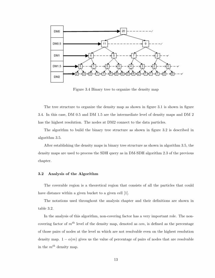
Figure 3.4 Binary tree to organize the density map

The tree structure to organize the density map as shown in figure 3.1 is shown in figure

3.4. In this case, DM 0.5 and DM 1.5 are the intermediate level of density maps and DM 2

has the highest resolution. The nodes at DM2 connect to the data particles.

The algorithm to build the binary tree structure as shown in figure 3.2 is described in

algorithm 3.5.

After establishing the density maps in binary tree structure as shown in algorithm 3.5, the

density maps are used to process the SDH query as in DM-SDH algorithm 2.3 of the previous

chapter.

3.2 Analysis of the Algorithm

The coverable region is a theoretical region that consists of all the particles that could

have distance within a given bucket to a given cell [1].

The notations used throughout the analysis chapter and their definitions are shown in

table 3.2.

In the analysis of this algorithm, non-covering factor has a very important role. The non-

covering factor of mth level of the density map, denoted as αm, is defined as the percentage

of those pairs of nodes at the level m which are not resolvable even on the highest resolution

density map. 1 − α(m) gives us the value of percentage of pairs of nodes that are resolvable

in the mth density map.

13

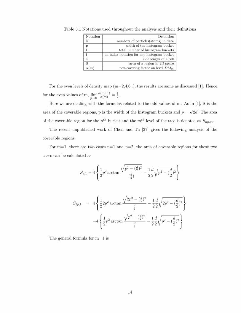
Table 3.1 Notations used throughout the analysis and their definitions

Notation Definition

N numbers of particles(atoms) in data

p width of the histogram bucket

L total number of histogram buckets

i an index notation for any histogram bucket

δ side length of a cell

S area of a region in 2D space

α(m) non-covering factor on level DMm

For the even levels of density map (m=2,4,6..), the results are same as discussed [1]. Hence

for the even values of m, limp→0

α(m+1)α(m) = 1

2 .

Here we are dealing with the formulas related to the odd values of m. As in [1], S is the

area of the coverable regions, p is the width of the histogram buckets and p =√

2d. The area

of the coverable region for the nth bucket and the mth level of the tree is denoted as Snp,m.

The recent unpublished work of Chen and Tu [37] gives the following analysis of the

coverable regions.

For m=1, there are two cases n=1 and n=2, the area of coverable regions for these two

cases can be calculated as

Sp,1 = 4

12p2 arctan

√p2 − (d2)2

(d2)− 1

2d

2

√p2 − (

d

2)2

S2p,1 = 4

12

2p2 arctan

√2p2 − (d2)2

d2

− 12d

2

√2p2 − (

d

2)2

−4

12p2 arctan

√p2 − (d2)2

d2

− 12d

2

√p2 − (

d

2)2

The general formula for m=1 is

14

Snp,1 = 4

12

(np)2 arctan

√(np)2 − (d2)2

d2

− 12d

2

√(np)2 − (

d

2)2

−4

12

((n− 1)p)2 arctan

√((n− 1)p)2 − (d2)2

d2

− 12d

2

√((n− 1)p)2 − (

d

2)2

For n=1 but m=3 and m=5 the formulas are:

Sp,3 = 4{

12p2π

2

}+ 2p(d− 2

d

4)

Sp,5 = 4{

12p2π

2

}+ 2p(d− 2

d

8) + 2p(d− 2

d

4) + (d− 2

d

8)(d− 2

d

4)

The general formula for n=1 is:

Sp,(2m+1) = 4{

12p2π

2

}+ 2p(d− 2

d

2m+1) + 2p(d− 2

d

2m)

+(d− 2d

2m+1)(d− 2

d

2m)

Similarly, for n=2 but m=3 and m=5, the formulas are:

S2p,3 = 4{

12

(2p)2π

2

}+ 2(2p)(d− 2

d

4)− 4

12p2 arctan

√p2 − d

4

2

d4

− 12d

4

√p2 − (

d

4)2

S2p,5 = 4{

12

(2p)2π

2

}+ 2(2p)(d− 2

d

8) + 2(2p)(d− 2

d

4) + (d− 2

d

8)(d− 2

d

4)

−4[12p2(

π

2− arctan

d2 −

d8√

p2 − (d2 −d8)2

)− 12

(

√p2 − (

d

2− d

8)2 − (

d

2− d

4)(d

2− d

8))

−12

(

√p2 − (

d

2− d

4)2 − (

d

2− d

8)(d

2− d

4))]

15

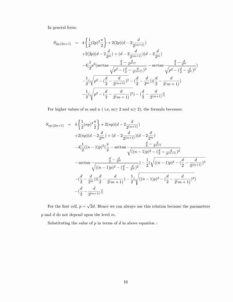
In general form:

S2p,(2m+1) = 4{

12

(2p)2π

2

}+ 2(2p)(d− 2

d

2(m+1))

+2(2p)(d− 2d

2m) + (d− 2

d

2(m+1))(d− 2

d

2m)

−4[12p2(arctan

d2 −

d2m+1√

p2 − (d2 −d

2(m+1) )2− arctan

d2 −

d2m√

p2 − (d2 −d

2m )2)

−12

(

√p2 − (

d

2− d

2(m+1))2 − (

d

2− d

2m))(d

2− d

2(m+ 1))

−12

(

√p2 − (

d

2− d

2(m+ 1))2)− (

d

2− d

2(m+1))]

For higher values of m and n ( i.e, m≥ 2 and n≥ 2), the formula becomes:

Snp,(2m+1) = 4{

12

(np)2π

2

}+ 2(np)(d− 2

d

2(m+1))

+2(np)(d− 2d

2m) + (d− 2

d

2(m+1))(d− 2

d

2m)

−4[12

((n− 1)p)2(π

2− arctan

d2 −

d2m+1√

((n− 1)p)2 − (d2 −d

2(m+1) )2

− arctand2 −

d2m√

((n− 1)p)2 − (d2 −d

2m )2)− 1

2(

√((n− 1)p)2 − (

d

2− d

2(m+1))2

−(d

2− d

2m))(d

2− d

2(m+ 1))− 1

2(

√((n− 1)p)2 − (

d

2− d

2(m+ 1))2)

−(d

2− d

2(m+1))]

For the first cell, p =√

2d. Hence we can always use this relation because the parameters

p and d do not depend upon the level m.

Substituting the value of p in terms of d in above equation :

16

Snp,(2m+1) = [2n2π + 2√

2n(1− 22m+1

) + 2√

2n(1− 22m

) + (1− 22m+1

)(1− 22m

)

−4[(n− 1)2(π

2− arctan

√2(n− 1)2 − (1

2 −1

2(m+1))2

12 −

12m+1

− arctan12 −

12m√

2(n− 1)2 − (12 −

12m )2

)− 12

(

√2(n− 1)2 − (

12− 1

2(m+ 1))2

−(12− 1

2m))(

12− 1

2(m+ 1))− 1

2(

√2(n− 1)2 − (

12− 1

2(m))2

−(12− 1

2(m+ 1)))(

12− 1

2(m))]]d2

The area of the coverable regions for all the buckets is denoted by f(n,m). It can be found

by using the above formulas of coverable region S as follows :

L∑n=1

f(n, 1) =[4L2 arctan

√8L2 − 1− 1

2

√8L2 − 1

]d2

(Substituting p =√

2d on the formula of Snp−1)

Similarly, from the formula of Snp,3

L∑n=1

f(n, 3) =[ L∑n=1

(2n2π +√

2n)

−∑n=2

L

[4(n− 1)2 arctan

√32(n− 1)2 − 1− 1

8

√32(n− 1)2 − 1

] ]d2

17

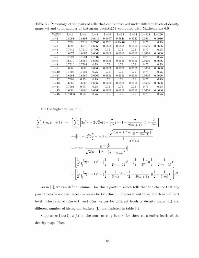
Table 3.2 Percentage of the pairs of cells that can be resolved under different levels of densitymaps(m) and total number of histogram buckets(L) computed with Mathematica 6.0

α(m+1)α(m)

L=2 L=4 L=8 L=16 L=32 L=64 L=128 L=256

m=1 0.8068 0.8898 0.9413 0.9697 0.9846 0.9922 0.9961 0.9980

m=2 0.7596 0.7522 0.7505 0.7501 0.75002 0.75 0.75 0.75

m=3 0.6696 0.6670 0.6666 0.6666 0.6666 0.6666 0.6666 0.6666

m=4 0.7545 0.7510 0.7502 0.75 0.75 0.75 0.75 0.75

m=5 0.6677 0.6667 0.6666 0.6666 0.6666 0.6666 0.6666 0.6666

m=6 0.7521 0.7504 0.7502 0.75 0.75 0.75 0.75 0.75

m=7 0.6670 0.6666 0.6666 0.6666 0.6666 0.6666 0.6666 0.6666

m=8 0.7510 0.7502 0.75 0.75 0.75 0.75 0.75 0.75

m=9 0.6668 0.6666 0.6666 0.6666 0.6666 0.6666 0.6666 0.6666

m=10 0.7505 0.7501 0.75 0.75 0.75 0.75 0.75 0.75

m=11 0.6668 0.6666 0.6666 0.6666 0.6666 0.6666 0.6666 0.6666

m=12 0.7502 0.75 0.75 0.75 0.75 0.75 0.75 0.75

m=13 0.6667 0.6666 0.6666 0.6666 0.6666 0.6666 0.6666 0.6666

m=14 0.7501 0.75 0.75 0.75 0.75 0.75 0.75 0.75

m=15 0.6666 0.6666 0.6666 0.6666 0.6666 0.6666 0.6666 0.6666

m=16 0.75006 0.75 0.75 0.75 0.75 0.75 0.75 0.75

For the higher values of m

L∑n=1

f(n, 2m+ 1) =[ L∑n=1

[2n2π + 2

√2n(1− 2

2m) + (1− 2

2(m+ 1))(1− 2

2m)]

−4[(n− 1)2(

π

2− arctan

√2(n− 1)2 − (1

2 −1

2(m+1))2

12 −

12(m+1)

− arctan12 −

12m√

2(n− 1)2 − (12 −

12(m)

)2)]

−

[12

(

√2(n− 1)2 − (

12− 1

2(m+ 1))2 − (

12− 1

2m))(

12− 1

2(m+ 1))

]

−

[12

(

√2(n− 1)2 − (

12− 1

2(m))2 − (

12− 1

2(m+ 1)))(

12− 1

2(m))

]]d2

As in [1], we can define Lemma 1 for this algorithm which tells that the chance that any

pair of cells is not resolvable decreases by two third in one level and three fourth in the next

level. The ratio of α(m+ 1) and α(m) values for different levels of density maps (m) and

different number of histogram buckets (L) are depicted in table 3.2.

Suppose α(1),α(2), α(3) be the non covering factors for three consecutive levels of the

density map. Then

18

α(2)α(1)

=23

α(3)α(2)

=34

This gives the ratio of α values for every alternate levels and that is:

α(3)α(1)

=12

The ratio of α values for every alternate levels is same as that the ratio of α values of the

two consecutive levels of the quad tree approach, as discussed in previous chapter. Therefore,

we can view the level between the two alternate levels as an intermediate level (assumem+0.5).

As depicted in figure 3.7,α(m+ 0.5)α(m)

=34

andα(m+ 1)α(m+ 0.5)

=23

givesα(m+ 1)α(m)

=12

With lemma 1, we can calculate the time complexity of the algorithm as follows:

Assume that there are I pairs of cells to be resolved on DMi. On next level, total number

of cell pairs becomes I × 2d.

According to lemma 1, 34 of them will be resolved leaving only I

3 × 2d+1 pairs to resolve.

On level DMi+2, 23 of 2d[ I3 × 2d+1] will be resolved. Here the number becomes I × 2(2d−1)

which is same as the value of DMi+1 in earlier algorithm with quad tree implementation.

In this way, the geometric progression becomes as follows:

I,I

3× 2d+1, I × 2(2d−1),

I

3× 23d, I × 22(2d−1), . . . ,

I

3× 2nd−

n−32 , I × 2

n2(2d−1) (3.1)

19

Sum = [I+I×2(2d−1)+I×22(2d−1)+. . .+I×2n2(2d−1)]+[

I

3×2d+1+

I

3×23d+. . .+

I

3×2nd−

n−32 ]

(3.2)

For the first geometric progression, the first term is I and the common ratio is 2(2d−1), so we

get the sum of the geometric progression as

Tc1(N) = I × ((2(2d−1))N+1

2 − 1)2(2d−1) − 1

(3.3)

One more level of density map will be built when N increases to 2dN . From equation 3.3 we

can get

Tc1(2dN) = 2(2d−1)Tc1(N)− o(1) (3.4)

From the second GP of equation 3.2, the first term = I3 × 2d+1 and common ratio = 22d−1,

hence the sum of the geometric progression is

Tc2(N) =I

3× 2d+1 × ((2(2d−1))

N−12 − 1)

2(2d−1) − 1(3.5)

Tc2(2dN) = 2(2d−1) × Tc1(N)− o(1) (3.6)

Applying master theorem, to equation 3.5 and equation 3.6 separately, we get

Tc1(N) = Θ(N2d−1d )

Tc2(N) = Θ(N2d−1d )

Since Total Time spent is the summation on equation 3.5 and equation 3.6, and the time

complexity of equation 3.5 and equation 3.6 are same, the time complexity of the operation

is Θ(N2d−1d ).

Our analysis says that the time complexity of the algorithm implementing binary tree is

same as that of the algorithm implementing quad-tree. It means that implementing binary tree

approach in DM-SDH algorithm does not really save time than the algorithm implementing

quad-tree approach. The advantage of the use of binary tree approach is that, if the cells are

20

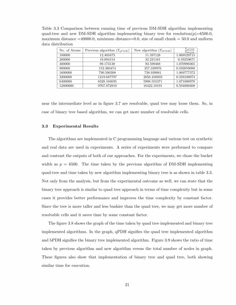
Table 3.3 Comparison between running time of previous DM-SDH algorithm implementingquad-tree and new DM-SDH algorithm implementing binary tree for resolution(p)=6500.0,maximum distance =40000.0, minimum distance=0.0, size of small chunk = 50.0 and uniformdata distribution

No. of Atoms Previous algorithm (TqPDH) New algorithm (TbPDH)TqP DH

TbP DH

100000 12.403473 11.597128 1.069529715

200000 19.094154 32.221161 0.59259671

400000 99.173138 92.599468 1.070990365

800000 152.360474 257.339976 0.592059098

1600000 790.500308 738.939081 1.069777372

3200000 1219.687797 2056.458933 0.593100974

6400000 6328.104035 5908.555371 1.071006978

12800000 9767.872919 16422.10191 0.594800408

near the intermediate level as in figure 3.7 are resolvable, quad tree may loose them. So, in

case of binary tree based algorithm, we can get more number of resolvable cells.

3.3 Experimental Results

The algorithms are implemented in C programming language and various test on synthetic

and real data are used in experiments. A series of experiments were performed to compare

and contrast the outputs of both of our approaches. For the experiments, we chose the bucket

width as p = 6500. The time taken by the previous algorithm of DM-SDH implementing

quad-tree and time taken by new algorithm implementing binary tree is as shown in table 3.3.

Not only from the analysis, but from the experimental outcome as well, we can state that the

binary tree approach is similar to quad tree approach in terms of time complexity but in some

cases it provides better performance and improves the time complexity by constant factor.

Since the tree is more taller and less bushier than the quad tree, we may get more number of

resolvable cells and it saves time by some constant factor.

The figure 3.8 shows the graph of the time taken by quad tree implemented and binary tree

implemented algorithms. In the graph, qPDH signifies the quad tree implemented algorithm

and bPDH signifies the binary tree implemented algorithm. Figure 3.9 shows the ratio of time

taken by previous algorithm and new algorithm versus the total number of nodes in graph.

These figures also show that implementation of binary tree and quad tree, both showing

similar time for execution.

21

Input: Consider xmin, ymin, xmax and ymax be the minimum and maximum x and ycoordinates

Initialize xspan and yspan as (xmax − xmin) and (ymax − ymin);if xspan is greater than yspan then

Partition the space horizontally;endelse

Partition the space vertically;endInitialize the xmin, xmax, ymin and ymax coordinates of firstdensity map as xlow, xhigh, ylow and yhigh respectively;for All the levels do

if the level is even thenfor All the nodes in that level do

Have the Coordinates of the parent node;Partition the space of the parent node into two equal halves verticallyand assign each of the space for the two children nodes;

endendelse

for All the nodes in that level doHave the coordinates of the parent node;Partition the space of the parent node into two equal halves horizontallyand assign each of the space for the two children nodes;if There are other nodes in the level then

Increment the currentnode pointerelse

Increment the parent pointerend

endend

endend

Figure 3.5 BuildBinaryTree() algorithm

22

Figure 3.6 A is the cell with bucket width p, bucket 1 is the region bounded by curves C1 toC8 and bucket 2 is the region bounded by curves D1 to D8 [1]

Figure 3.7 Conceptual tree structure with three density maps where the hidden line signifiesthe intermediate density map

23

Figure 3.8 Time taken by quad tree implemented algorithm (qPDH) and binary tree imple-mented algorithm (bPDH) vs number of nodes (in x axis)

Figure 3.9 Ratio of the time taken by previous algorithm and new algorithm (in y axis) vsnumber of nodes (in x axis)

24

CHAPTER 4

INSPECTING UNIFORM REGIONS HOPING TO IMPROVE THEPERFORMANCE

It is found that although we hoped to save some time implementing binary tree approach

of SDH initially, it is same as quad tree based approach in terms of time complexity. In search

for the means of further improvements of spatial histogram, in this chapter, it is proposed

that if we could find some uniform regions in the tree, the algorithm can be more improved.

Consider two cells A and B, if we could conclude that A and B are uniform regions in the

tree, we do not need to figure out whether A and B are resolvable or not, and we do not need

to compute the point-to-point distance among the particles in those uniform regions even if

A and Bare irresolvable and at the highest resolution level of the density map. We can have

the distance distribution function of those uniform cells and find the distance histogram using

that distribution function. Since determining whether the two cells resolve or not and finding

the point-to-point distances among the particles are the two major operations of the DM-SDH

algorithm, on which the algorithm spends a lot of time, the time would definitely be saved if

we could skip the major operations for some of the cells.

4.1 The Goodness of Fit Test

The chi-square test is popularly used in those experiments in which data is frequency or

counts [16].The goodness of fit test to any statistical test (like Chi square test, Kolmogorov

Smirnov test and so on) describes how well it fits in the sets of observations. In our case,

on calculating the p-value implementing Chi-Square test, if the p-value is greater than some

specific constant value we consider the node is uniform otherwise the node is not. If the

node B as in figure 4.1 is uniform all the children of node B (as depicted in the figure by the

triangle) are also uniform and we do not need to calculate the point-to-point distances among

25

Figure 4.1 If B is uniform, the children nodes of B are also uniform

Figure 4.2 If B is uniform, the cells in B are also uniform

those uniform nodes. It can also be described as in figure 4.2, if B is the uniform cell in the

tree, all the cells inside B are also uniform.

The test statistics of Chi-square test can be represented by the equation given below:

χ2 =∑n

i=1(Oi−Ei)2

E2i

where

χ2 = the test statistic that asymptotically approaches a chi-square distribution.

Oi= an observed frequency.

Ei = an expected (theoretical) frequency as given by the null hypothesis.

n = the number of particles(in our terms) in each node.

26

4.2 R - for Statistical Computing

R is a statistical computing tool which have been extensively used by statisticians and

bio-statisticians. It is developed at Bell laboratories by John Chambers and colleagues [36].

R provides a wide range of statistical functions which are highly extensible as well. In this

thesis, we have used R to implement the Chi-Square test. We have used the stand-alone

version of math library from R to C.

Input: Say node be the input node, and level be the respective level of that nodefor all the available nodes do

totalcount = calculate the total number of particles;endDOF = 4level − 1;expected = totalcount

DOF ;t = i;while t has children do

for Each child k of t doobserved = the particles contained by k ;chisqval = chisqval + (observed−expected)2

expected2;

endt=first child of t;

endpval = pchisq(chisqval,DOF, TRUE,FALSE);If pval ≤ 0.1 Return 1 ;Else Return 0;

Figure 4.3 FindingUniformRegions() algorithm

In the algorithm 4.3, we have presented the idea of how can we find the uniform regions,

using chi-square test. At every level of the density map, the degree of freedom changes as

(total number of nodes on that level − 1) because at every level the number of total nodes

also change, the constant factor to compare the p-value we have chosen is 0.1. pchisq() is the

function of the stand-alone library of R. A series of experimental analysis could be done to

find out an appropriate constant factor. The general chi-square distribution table is shown in

figure 4.4.

Table 4.2 shows the number of uniform regions detected for 500,000 number of input

atoms. We can figure out that as we go to the lower level, we can find higher percentage of

number of uniform regions. Another discovery is that starting from the level 3 (with 64 cells),

27

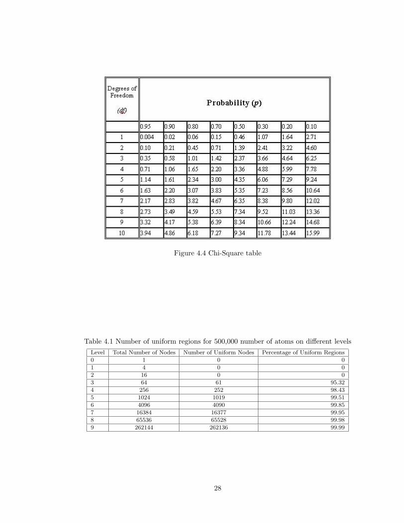
Figure 4.4 Chi-Square table

Table 4.1 Number of uniform regions for 500,000 number of atoms on different levelsLevel Total Number of Nodes Number of Uniform Nodes Percentage of Uniform Regions

0 1 0 0

1 4 0 0

2 16 0 0

3 64 61 95.32

4 256 252 98.43

5 1024 1019 99.51

6 4096 4090 99.85

7 16384 16377 99.95

8 65536 65528 99.98

9 262144 262136 99.99

28

we can see a high percentage of uniform nodes that give a high percentage of the uniform

regions. This means that most of the high level regions can be treated as a single entity in

the approximate algorithm, that means for those regions (for 61 nodes in the level 3) we do

not need to calculate the point to point distances and we do not need to find out whether the

cells are uniform or not. Thus, it greatly reduces the computation time. After finding the

uniform regions as shown in algorithm 4.3. It would be very interesting to analyze the time

complexity of our algorithm after implementing the idea of inspection of the uniform regions.

It can be considered as an immediate future work of this research.

29

CHAPTER 5

CONCLUSION AND FUTURE ENHANCEMENTS

5.1 Conclusion

SDH was first implemented in quad-tree, and we did not know whether that was the opti-

mal algorithm or not. In this thesis, we have shown the another approach of the computation

of SDH using binary tree approach. The binary tree approach has the time complexity of

θ(N2d−1d ) where d is the dimension. In this thesis, we are dealing with the two dimensional

data only, so the time complexity of the program for d = 2 is θ(N32 ). This approach is def-

initely faster than the brute force approach. Our experimental results show that the time

complexity of the algorithm using quad-tree approach is same as that of the algorithm using

the binary tree approach. In some cases, binary tree approach does provide improvement of

time by a constant factor.

This thesis presents an idea of implementation of binary tree in the density maps and

hence implementation of rectangular cell shape in the DM-SDH concept.

This thesis also deals with some statistical tests on the data contained by the tree. The

uniform nodes are found out using the chi-square test. Our intuition says that if we would

implement the idea of the uniform regions in the DM-SDH algorithm, we could be able to

improve the algorithm in terms of time, since most of the high level regions, due to the

uniformly distributed particles, can be treated as a single entity in the approximate algorithm.

Analyzing the time complexity after inspecting the uniform regions is beyond the scope of this

thesis.

5.2 Future Enhancements

Although there are many relational database systems, none of them are working perfectly

in the field of storing and analyzing scientific particles data, because they are particularly

30

designed to store, analyze and handle with the data in business environment.There can be so

many ways to enhance the concept of “Spatial Distance Histogram”. We can also implement

this concept in various other types of trees to find out the optimal solution. The space

partitioning methods with cell shapes other than square (as dealt in quad tree) and rectangle

(as dealt in binary tree) can also be implemented.

In case of DM-SDH algorithm, we compute the distance between all the irresolvable par-

ticles at the highest resolution level. By implementing the novel idea of uniform regions, we

may decrease the no. of computations, and hence improve the efficiency. As already discussed

in previous chapter, calculation of time taken by the algorithm by experimental and analytic

means would be considered as an immediate future work.

In this thesis, the optimization of the algorithm based upon I/O costs are not discussed.

The algorithm could certainly be improved if the advantages of pre-fetching mechanism could

be implemented. The ways to improve the I/O performance of algorithm can also be studied.

31

REFERENCES

[1] Y-C.Tu, S. Chen, and S. Pandit ”Computing Spatial Distance Histograms Efficiently inScientific Databases”, Department of Computer Science and Engineering, University ofSouth Florida, 2008.

[2] H. Samet, ”The Design and Analysis of Spatial Data Structures”, University of Maryland,Addison-Wesley, Reading, MA, 1990.

[3] D. Frenkel and B. Smit, ”Understanding Molecular Simulations from Algorithm to Ap-plications”, ser. Computational Science Series. Academic Press, 2002, vol. 1.

[4] J. Gray, D. Liu, M. Nieto-Santisteban, A. Szalay, D. DeWitt, and G. Heber, ”ScientificData Management in the Coming Decade”, SIG MOD Record, vol. 34, no. 4, Dec. 2005.

[5] Y-C. Tu and S. Chen ”Performance Analysis of Dual-Tree Algorithms for ComputingDistance Histograms”

[6] P.N. Yianilos, ”Data Structures and Algorithms for Nearest Neighbor Search in MetricSpaces” in Proceedings of ACM-SIAM Symposium on Discrete Algorithms(SODA), 1993

[7] M.A. Nieto-Santisteban, J. Gray, A.S. Szalay, J. Annis, A.R. Thakar, and W.J.O’Mullane, ”When Database Systems Meet the Grid” Proceedings of the 2005 CIDRConference

[8] R. Agrawal, A. Ailamaki, P. A. Bernstein, E. A. Brewer, M. J. Carey, S. Chaudhuri,A. Doan, D. Florescu, M. J. Franklin, H. Garcia-Molina, J. Gehrke, L. Gruenwald, L.M. Haas, A. Y. Halevy, J. M. Hellerstein, Y. E. Ioannidis, H. F. Korth, D. Kossmann,S. Mad- den, R. Magoulas, B. C. Ooi, T. O’Reilly, R. Ramakrishnan, S. Sarawagi, M.Stonebraker, A. S. Szalay, and G. Weikum, ”The claremont report on database research,”Commun.ACM, vol. 52, no. 6, pp. 56-65, 2009.

[9] M.Y. Eltabakh, M.Ouzzani, W.G. Aref, ”bdbms - A Database Management System forBiological Data”, 3rd Biennial Conference on Innovative Data Systems Research (CIDR)January 7-10, 2007, Asilomar, California, USA.

[10] J.M. Patel,”The Role of Declarative Querying in Bioinformatics”, OMICS A Journal ofIntegrative Biology, Volume 7, Number 1, 2003, Mary Ann Liebert, Inc.

[11] B. Nam, A. Sussman, ”A Comparative Study of Spatial Indexing Techniques for Mul-tidimensional Scientific Datasets”, Proceedings of the 16th International Conference onScientific and Statistical Database Management (SSDBM04) 1099-3371/04 2004 IEEE

[12] I. Narsky, ”Goodness of Fit: What Do We Really Want to Know?”, PHYSTAT2003,SLAC, Stanford, California, September 8-11, 2003

32

[13] M.H. Ng,S. Johnston, B. Wu, S.E. Murdock, K. Tai, H. Fangohr, S.J. Cox, J.W. Es-sex,M.S.P. Sansom, P.Jeffreys, ”BioSimGrid: Grid-enabled biomolecular simulation datastorage and analysis ” Future Generation Computer Systems 22 (2006) 657664

[14] C.W. Bachman, ”DATA STRUCTURE DIAGRAMS”, Journal of ACM SIGBDP Vol 1No 2 (March 1969) pages 4-10.

[15] B. Chan,J. Talbot, L. Wu, N. Sakunkoo, M. Cammarano, P. Hanrahan, ”Vispedia: On-demand Data Integration for Interactive Visualization and Exploration ”, SIGMOD09,June 29July 2, 2009, Providence, Rhode Island, USA. ACM 978-1-60558-551-2/09/06.

[16] A.E. Maxwell, ”Analysing Qualitative Data”, 1961

[17] S.L. Meyer, ”Data Analysis for Scientists and Engineers”, 1975

[18] A. S. Szalay, J. Gray, A. Thakar, P. Z. Kunszt, T. Malik, J. Raddick, C. Stoughton, andJ. vandenBerg, The SDSS Skyserver: Public Access to the Sloan Digital Sky Server Data,in Proceedings of International Conference on Management of Data (SIGMOD), 2002,pp. 570581.

[19] J. L. Stark and F. Murtagh, Astronomical Image and Data Analysis. Springer, 2002.

[20] A. Filipponi, The radial distribution function probed by Xray absorption spectroscopy,J. Phys.: Condens. Matter, vol. 6, pp. 84158427, 1994.

[21] V. Springel, S. D. M. White, A. Jenkins, C. S. Frenk, N. Yoshida, L. Gao, J. Navarro,R. Thacker, D. Croton, J. Helly, J. A. Peacock, S. Cole, P. Thomas, H. Couchman,A. Evrard, J. Colberg, and F. Pearce, Simulations of the Formation, Evolution andClustering of Galaxies and Quasars, Nature, vol. 435, pp. 629636, June 2005.

[22] J. A. Orenstein, Multidimensional Tries used for Associative Searching, Information Pro-cessing Letters, vol. 14, no. 4, pp. 150157, 1982.

[23] Y. Tao, J. Sun, and D. Papadias, Analysis of predictive spatio-temporal queries, ACMTrans. Database Syst., vol. 28, no. 4, pp. 295336, 2003.

[24] I. Csabai, M. Trencseni, L. Dobos, P. Jozsa, G. Herczegh, N. Purger, T. Budavari, and A.S. Szalay, Spatial Indexing of Large Multidimensional Databases, in Proceedings of the3rd Biennial Conference on Innovative Data Systems Resarch (CIDR), 2007, pp. 207218.

[25] M. Arya, W. F. Cody, C. Faloutsos, J. Richardson, and A. Toya, QBISM: Extending aDBMS to Support 3D MedFical Images, in ICDE, 1994, pp. 314325.

[26] B. Hess, C. Kutzner, D. van der Spoel, and E. Lindahl, GROMACS 4: Algorithms forHighly Efficient, Load-Balanced, and Scalable Molecular Simulation, Journal of ChemicalTheory and Computation, vol. 4, no. 3, pp. 435447, March 2008.

[27] M. Feig, M. Abdullah, L. Johnsson, and B. M. Pettitt, Large Scale Distributed DataRepository: Design of a Molecular Dynamics Trajectory Database, Future GenerationComputer Systems, vol. 16, no. 1, pp. 101110, January 1999.

[28] M.P. Allen and D.J.Tildesley, ”Computer Simulation of Liquids”. Clarendon Press, 2002,vol.1.

33

[29] J.M. Haile ”Molecular Dynamics Simulation: Elementary Methods”. Wiley, New York,1992.

[30] D.P. Landau and K. Binder. ”A Guide to Monte Carlo Simulation in Statistical Physics”.Cambridge University Press, Cambridge, 2000.

[31] M. Bamdad, S. Alavi, B. Najafi, and E. Keshavarzi, ” A new expression for radial dis-tribution function and infinite shear modulus of lennard-jones fluids”, Chem. Phys. Vol.325, pp. 554-562, 2006.

[32] Y-C.Tu, S. Chen, and S. Pandit ”Computing Spatial Distance Histograms Efficiently inScientific Databases”, In Proceedings of International Conference on Data Engineering(ICDE), pages 726-807, March 2009.

[33] J. K. Uhlman, Metric Trees, Applied Mathematics Letters, vol. 4, no. 5, pp. 6162, 1991.

[34] J. Barnes and P. Hut ”A Hierarchical O(N logN) Force Calculation Algorithm”. Nature,324(4):446-449,1986

[35] P.B. Callahan and S.R. Kosaraju, ”A decomposition of multidimensional point setswith applications to k-nearest neighbors and n-body potential fields”. Journal od ACM,42(1):67-90,1995.

[36] R-resources and tutorials, website link: http://www.r-project.org/

[37] S. Chen, Y. Tu. Personal communication.

[38] Chi-Square table, website link: http://www2.lv.psu.edu/jxm57/irp/chisquar.html

34