Performance analysis and formal verification ofcognitive wireless networks

G.L. Dei Rossi, L. Gallina, and S. Rossi

Universita Ca’ Foscari, Venezia (Italy){deirossi,lgallina,srossi}@dais.unive.it

Abstract. Cognitive Networks are a class of communication networks,in which nodes can learn how to adjust their behaviour according tothe present and past network conditions. In this paper we introducea formal probabilistic model for the analysis of wireless networks in whichnodes are seen as processes capable of adapting their course of actionto the environmental conditions. In particular, we model a network madeof mobile nodes using the gossip protocol, and we study how the energyperformance of the network varies, according to the topology changes andthe transmission power. The stochastic process underlying the model isa discrete time Markov chain. We use the PRISM model checker to obta-in, through Monte-Carlo simulation, numerical results for our analysis,which show how the learning-driven dynamic adjustment of transmissionpower can improve the energy performance while preserving connectivity.

1 Introduction

Cognitive networks [4] are communication networks in which nodes can altertheir behaviour according to changes of the environmental conditions. Whatdifferentiate this approach from the one of cognitive radio [8] networks are that,while in the latter the choices that nodes can take are restricted to radio channelselection, in the former nodes can take complex decisions, taking into accountthe global goals of the network. Cognitive processes are particularly useful whenwe have to deal with ad hoc networks, where the absence of a fixed infrastructureand the dynamic nature of the network topology, as well as the limited powercapacities of nodes, make the network prone to problems such as link breakages,energy waste and interferences.

Topology Control is a technique aimed at guaranteeing network connectivity,while optimising network performance with respect to several metrics, dependingon the specific objective of each single network.

Although several formal models for the analysis of wireless ad hoc and sensornetworks and for cognitive radio networks were proposed in the literature (see,e.g., [13, 5]), to the best of our knowledge formal models for the analysis ofcognitive networks are rare. In [9] the authors discuss the issues concerning thedefinition of a PEPA model for cognitive networks, although they do not proposeany actual model, and thus they do not perform any quantitative or qualitativeanalysis.

PRISM [10] is a tool for modelling and analysing systems that exhibit a prob-abilistic behaviour. It supports, among others, the modelling of Markov DecisionProcesses (MDPs), where nondeterministic and probabilistic aspects coexist. Inaddition to the traditional model checking, PRISM provides statistical modelchecking, allowing one to compute probabilities of properties’ satisfaction. Inparticular, PRISM also offers a discrete-event simulator, allowing one to gener-ate approximate results for the verification of properties. This approach is par-ticularly useful for very large models, when other approaches to model checkingare not feasible, due to the well known problem of state space explosion.

This paper presents a probabilistic model for the analysis of networks ex-hibiting cognitive behaviours. The model is written in the PRISM language, andsupports broadcast communications, node mobility, and the ability of nodes todynamically adjust the transmission power during their operations.

Paper structure. The paper is organised as follows. In Section 2 we givean introduction to the use of cognitive networks for topology control, Section3 reviews the basic features of PRISM that we use in the rest of the paper. InSection 4 we introduce a novel model for cognitive networks, and in Section 5 weuse the PRISM tool to analyse its behaviour, giving numerical examples. Finally,in Section 6 we give some final remarks, concluding the paper.

2 Topology Control with Cognitive Networks

Topology Control [14] is a technique aimed at guaranteeing the connectivityof a communication network, while limiting other cost factors, such as the levelof interference and the energy consumption, thus extending the network lifetime.In the presence of mobility this problem is not trivial, since the network topol-ogy continuously changes, causing frequent link breakages and variations in theinterference levels. In wireless networks, this can be considered as the problem offinding a trade-off between power saving and network connectivity through thechoice of the appropriate transmission power for each node. It is evident that ifeach node transmits at a low power, then its connectivity level, and potentiallythe one of the whole network, will be reduced, while if we assign high transmis-sion power to the nodes, we generally enhance the connectivity of the network,but we consume far more energy. This relation is, indeed, not a trivial one, sinceincreasing transmission power, and thus the coverage area of a radio station, canincrease the chances of collisions and interferences, decreasing the whole networkconnectivity. For omni-directional antennas we can reasonably model the cover-age radius as a function of the power used by the transmitter, and vice-versa.The function can be arbitrary, but usually the coverage radius is proportionalto the square root of the transmission power [12]. Of course connectivity is alsoinfluenced by factors independent from the transmission power, such as routingand link-level protocols. However in this paper we focus on energy consump-tion, leaving all the other factors unchanged. In particular, we assume that thenetwork uses the well-known gossip protocol to propagate messages.

2

In this article we also assume that every node in the network is somewhatsmart, and capable of applying some strategies to decide its transmission power,based on the conditions in which it operates. In particular, we assume that,observing the past behaviour of the network, or using some link-level techniquesusually employed for interference, collision and congestion detection [17], eachnode is able to guess how many other stations are present in a given radius.Given that information, the node can perform a very simple decision, i.e.,

– If there is a radius r < rmax for which there are at least n other nodes, usethe minimum transmission power capable of transmitting with radius r.

– Use the maximum allowed power, corresponding to radius rmax, otherwise.

It is clear that, due to mobility and interferences, the guess of the aforemen-tioned node can be wrong, however this mistake will have an effect on the nextretransmissions of the node itself. In this way, we have just defined a cognitivenetwork in which nodes are able to learn, from the observed environment, anappropriate behaviour for the net itself.

3 The PRISM Model Checker

PRISM [10] is a probabilistic model checker which supports several types ofmodels, such as discrete-time Markov chains (DTMCs), continuous-time Markovchains (CTMCs), Markov decision processes (MDPs), and Probabilistic TimedAutomata (PTA). Models are expressed using PRISM’s own language.

This paper deals with models that can be represented by Discrete TimeMarkov Chains [15], and studies their qualitative and quantitative propertiesusing model checking techniques. In the following we briefly introduce the mainaspects of the PRISM language.

3.1 Modules.

PRISM models consist of modules, expressed through a simple state-basedlanguage. A module is specified as:

module name

...

endmodule

and it is composed of variables and commands. Variables are names associatedto values. The syntax for variables is:

name : [ range ] init initial_value;

Commands describe all the possible behaviours of the modules, i.e. all the pos-sible transitions from one state to another. They include guards, which indicatethe states where the transitions can occur, and the updates, which modify thevariables in order to reach the arrival states. The syntax for a command is:

3

[action] guards -> p1:update1 + p2:update2 .. pn:updaten;

where p1, ..., pn express the probability of each possible update (∑n

i=1pi = 1),guards is the list of conditions associated to that transitions, and action is thelabel of the transitions, which is used to synchronise different modules, since twomodules can synchronise if they can execute an action with the same label.

3.2 The Property Specification Language

PRISM provides a specification language to express rewards and quantita-tive properties and it supports the automated analysis of these properties withrespect to the probabilistic models. It supports several temporal logics, suchas PCTL (Probabilistic Computation Tree Logic) and LTL (Linear TemporalLogic) [7]. In particular, when dealing with DTMCs, the PRISM property spec-ification language enables us to study many important properties, such as theprobability to reach a particular state under some conditions.

The P operator is used to reason about the probability of the occurrence ofan event. Formally, we write:

P bound [ pathprop ]

which is true if the probability that the path property pathprop is satisfied bythe paths reachable from the initial states respects the bound bound.

We can also adopt a quantitative approach, by computing the actual proba-bility that a path property is satisfied. An example is:

P =? [pathprop]

which computes the probability of satisfying pathprop.The PRISM property specification language introduces a set of temporal op-

erators in order to express the PCTL path formulas or the LTL formulas whichcan be verified for a single path of a model. Among these operators, the mostused are F, which expresses the property that the condition will be eventuallysatisfied by the path, and G which expresses the property that the condition isalways true (i.e., it expresses the invariancy property).

3.3 Costs and Rewards.

Reward properties are based on the possibility of defining rewards associatedwith a given PRISM model. Rewards can assign values, or costs, either to statesor transitions. We are interested in transitions rewards, whose syntax is:

rewards ‘‘name’’

[action_1] constraint_1 : cost_1

[action_2] constraint_2 : cost_2

...

[action_n]constraint_n : cost_n

endrewards

4

where, for each i ∈ [1 − n] assigns the cost cost i to the transitions labelledwith [action i] satisfying the constraint constraint i.

With the PRISM property specification language we can use the R operatorto compute the expected value of the rewards associated with the model. As forthe reachability properties (the P operator), we can verify if the cost of reachingthe states satisfying some particular property respects a certain bound:

R bound [ rewardprop ]

We can also compute the expected cost of reaching states satisfying a givenproperty:

R = ? [F rewardprop]

3.4 Statistical Model Checking

Due to the well-known problem of state space explosion, in addition to thestandard model checking techniques, which need to build the entire model for theverification of properties, PRISM also provides a discrete-event simulator, whichcan be used to perform approximate (or statistical) model checking. Approximateresults can be obtained by generating a large number of paths through the model,without building the entire state space, evaluating the properties on each run,and using the information to generate approximate results. This technique canbe used to analyse both reachability and reward properties, and it is particularlyuseful to study models with a large number of modules and interactions (see [11]).

4 The Model

We consider a wireless network with both static and mobile devices, wherecommunications are carried on using a basic gossip protocol. Nodes can, throughradio-frequency channels, broadcast messages, which are receivable by all thenodes which are inside the sender node’s transmission area and are listening tothe same channel. We analyse the energy costs of a multi-hop communicationbetween two random network nodes, and we study how the ability of learningand reasoning in the processes behaviour can improve the performance of thenetwork.

In particular, we model 15 mobile nodes, and 10 static nodes, evenly dis-tributed in a network area of 50×100 square meters, as depicted in Figure 1.The static nodes are located at positions {7, 9, 17, 19, 27, 29, 37, 39, 47, 49}, whilethe movements for all the other nodes are described by the bidirectional arrowsin Figure 1. We model the network area as a grid of 5×10 cells. The distancesbetween cells are determined by considering the centre of each cell and calcu-lating the euclidean distance between each pair of centres (each cell is 10 × 10square metres). Moreover, we consider each node as a cognitive process, that candynamically change the transmission power for its communications, dependingon the position of its active neighbours, with the global aim of an efficient topol-ogy control. Usually, modern technologies allow the devices to choose among a

5

1

4

5

3

2

6

9

10

8

7

11

14

15

13

12

16

19

20

18

17

21

24

25

23

22

26

29

30

28

27

31

34

35

33

32

36

39

40

38

37

41

44

45

43

42

46

49

50

48

47

Fig. 1: Topology of the Network

discrete set of possible power levels. In what follows we will use the transmissionradius to represent the transmission power, since those quantities are strictly re-lated. As we mentioned in Section 2, usually the power spent for a transmission isproportional to the squared radius. The processes that model nodes listen to thechannel and, when they receive a message, they forward it, according to the gos-sip strategy, i.e., they will forward the message with a certain probability psend,and discard it with probability 1 − psend. We will study the performance ofthe network, for different gossip strategies, i.e., with the value of the forwardingprobability ranging in the set {0.65, 0.7, 0.75, 0.8, 0.85, 0.9, 0.95, 1.0}.

Several papers, such as [6, 1–3], already present analysis of gossip-based pro-tocols, comparing modifications which are particularly appropriate for ad hocand wireless networks. In this paper we analyse how the presence of cognitiveprocesses in the network can strongly improve the performance of these kinds ofcommunication protocols. In our model, each node can choose its transmissionradius in the set {10m, 15m, 20m}. Specifically, it will choose the minimum ra-dius which ensure the possibility to receive the message for at least two receiversor, if there are not enough available neighbours in the transmission area, it willtransmit with its maximum power ( radius = 20m).

As introduced in Section 3, the PRISM model checker supports differentmodel types. Here we model the network as a DTMC, where probabilities areused to model both the possible topology changes, and the behaviour of theprocesses. In what follows we will give the essential elements of the mapping ofthe aforementioned model in PRISM’s own language. Table 1 shows the repre-sentation of a single network node.

Variables. The most important variables of our model mapping are the following:

– stepsi controls the sequentiality of the process executed by the sensor nodei. In particular, stepsi = 2 means that the node is ready to receive, stepsi =1 means that the node is ready to transmit, and stepsi = 0 means that thenode has completed a transmission.

– li: is the variable containing the actual location of the sensor node i.

6

Table 1: The PRISM module for a node

module P8steps8 : [0 .. 2] init 2;l8 : [15 .. 20] init 15;

[move] (l8 = 15) → 0.8 : (l8′ = 20) + 0.8 : (l8′ = 15);[movee] (l8 = 20) → 0.8 : (l8′ = 15) + 0.8 : (l8′ = 20);

//beginning of a new round[round] no one sending → (steps8′ = 2);

//transmission//[c8] (steps8 = 1)→ (steps8′ = 0);

//reception[c3] (steps8 = 2)& s1p3 & s1p38→ psend : (steps8′ = 1) + (1− psend) : (steps8′ = 0);[c3] (steps8 = 2)& s2p3 & s2p38→ psend : (steps8′ = 1) + (1− psend) : (steps8′ = 0);[c3] (steps8 = 2)& s3p3 & s3p38→ psend : (steps8′ = 1) + (1− psend) : (steps8′ = 0);[c3] (steps8! = 2) |!((s1p3 & s1p38) | (s2p3 & s2p38) | (s3p3 & s3p38))→ (steps8′ = steps8)

[c5] (steps8 = 2)& s2p5 & s2p58→ psend : (steps8′ = 1) + (1− psend) : (steps8′ = 0);[c5] (steps8 = 2)& s3p5 & s3p58→ psend : (steps8′ = 1) + (1− psend) : (steps8′ = 0);[c5] (steps8! = 2) |!((s2p5 & s2p58) | (s3p5 & s3p58))→ (steps8′ = steps8)

[c7] (steps8 = 2) & s1p7 & s1p78→ psend : (steps8′ = 1) + (1− psend) : (steps8′ = 0);[c7] (steps8 = 2) & s2p7 & s2p78→ psend : (steps8′ = 1) + (1− psend) : (steps8′ = 0);[c7] (steps8 = 2) & s3p7 & s3p78→ psend : (steps8′ = 1) + (1− psend) : (steps8′ = 0);[c7] (steps8! = 2) |!((s1p7 & s1p78) | (s2p7 & s2p78) | (s3p7 & s3p78))→ (steps8′ = steps8)

[c10] (steps8 = 2) & s1p10 & s1p108→ psend : (steps8′ = 1) + (1− psend) : (steps8′ = 0);[c10] (steps8 = 2) & s2p10 & s2p108→ psend : (steps8′ = 1) + (1− psend) : (steps8′ = 0);[c10] (steps8 = 2) & s3p10 & s3p108→ psend : (steps8′ = 1) + (1− psend) : (steps8′ = 0);[c10] (steps8! = 2) |!((s1p10 & s1p108) | (s2p10 & s2p108) | (s3p10 & s3p108))→ (steps8′ = steps8)

[c12] (steps8 = 2)& s2p12 & s2p128→ psend : (steps8′ = 1) + (1− psend) : (steps8′ = 0);[c12] (steps8 = 2)& s3p12 & s3p128→ psend : (steps8′ = 1) + (1− psend) : (steps8′ = 0);[c12] (steps8! = 2) |!((s2p12 & s2p128) | (s3p12 & s3p128))→ (steps8′ = steps8)

[c13] (steps8 = 2)& s1p13 & s1p138 → psend : (steps8′ = 1) + (1− psend) : (steps8′ = 0);[c13] (steps8 = 2)& s2p13 & s2p138 → psend : (steps8′ = 1) + (1− psend) : (steps8′ = 0);[c13] (steps8 = 2)& s3p13 & s3p138 → psend : (steps8′ = 1) + (1− psend) : (steps8′ = 0);[c13] (steps8! = 2) |!((s1p13 & s1p138) | (s2p13 & s2p138) | (s3p13 & s3p138)) → (steps8′ = steps8)

endmodule

7

Table 2: Connectivity formulas

//P1 strategiesformula s1p12 = ((steps2 = 2) & (l2− l1 = 1));formula s1p14 = ((steps4 = 2) & (l4 = l1− 5));

formula s2p12 = s1p12;formula s2p14 = (steps4 = 2);formula s2p15 = ((steps5 = 2) & (l5− l1 = 6));

formula s3p12 = ((steps2 = 2) & (l2− l1 < 3));formula s3p14 = (steps4 = 2);formula s3p15 = s2p15;formula s3p16 = ((steps6 = 2) & (l6− l1 = 10));

formula s1p1 = (s1p12 & s1p14);formula s2p1 =!s1p1 & ((s2p12 & s2p14) | (s2p12 & s2p15) | (s2p14 & s2p15));formula s3p1 =!s1p1 & !s2p1;

Modelling the Network Topology. In order to model the level of connectivity ofthe network, which dynamically changes depending on the positions of the nodesinside the network area, and before defining the modules for the network nodes,we introduce a list of formulas, which allow us to verify the distance betweeneach pair of possible neighbours. In particular, for each pair i, j ∈ {1, ..., 25} andfor each h ∈ {2, 3, 4}, if the formula shpij is true, it means that the node Pj

is actually able to listen to a Pi’s transmission with radius 5× h. Moreover, foreach i ∈ {1, ..., 25} and for h ∈ {2, 3, 4}, if the formula shpi is true, then thereexists at least two possible receiver nodes inside the transmission area of thesender, when transmitting with radius 5× h. Table 2 shows the set of formulasmodelling the connectivity of P1. As an example,

formula s1p12 = ((steps2 = 2) & (l2− l1 = 1));

is true when node P2 is ready to receive (steps2 = 1), and the distance betweenP1 and P2 is 1, i.e., looking at Figure 1, is true only when l1 = 2 and l2 = 3,which, since we consider the nodes lying in the centre of each cell, means thatradius 10m guarantees their connection.

Transitions.

– [move]: is the transition modelling the periodic topology changes. Node mo-bility is expressed in terms of the transition matrix of a discrete time markovchain: each entry of the matrix denotes the probability that a sensor nodemoves from a location to another. In particular, static nodes are associatedwith the identity m atrix. When the transition move is performed, a nodewill change location with probability ε, and will remain in the same locationwith probability 1− ε. Here we choose 0.8 as the value for ε.

8

– [round]: is the transition occurring when no more transmissions are possible.At the end all the nodes will be in the reception state (stepsi = 2), exceptfor the sender node, whose steps variable will be set to 1.

– [ci]: is the transition modelling a broadcast trasmission. In particular, ifa node is in the state ready to transmit (stepsi = 1), it will execute thefollowing transition:

[ci] (stepsi = 1)→ (stepsi′ = 0);

meaning that the node i transmits the message and then transits in a sleepingphase. If another node Pj is in the state ready to transmit (stepsj = 2), andit is inside the transmission area of the sender node (s1pij, s2pij, s3pij), itwill synchronize with the sender node and receive the message. Transition [ci](stepsj = 2)&s1pi&s1pij→ psend : (stepsj′ = 1) + (1− psend) : (stepsj′ = 0);

models the basic gossip strategy: the node receiving the message will forward itwith probability psend, and discard it with probability 1− psend.

Rewards. As introduced in Section 3, PRISM allows us to specify rewards (orcosts), associated to both states and transitions. In order to study the energyperformance of the networks, we associate a cost to each transition. In particular,for each transition [ci] (meaning that Pi is sending a message) we verify whichtransmission power has been used for the transmission (s1p1, s2p1 or s3p1),and we use the values 1 for radius 10 m, 1.5 for radius 15m and 2 for radius20m.

We are interested also in studying how many retransmissions the sender mustperform before the communication is successfully completed. In order to do so,we introduce another reward, simply assigning 1 to each transition tagged with[round].

Formally, rewards are written as follows:

rewards "rounds"

[round] true : 1;

endrewards

rewards "costs"

[c1] s1p1 : 1;

[c1] s2p1 : 1.5;

[c1] s3p1 : 2;

[c2] s1p2 : 1;

[c2] s2p2 : 1.5;

[c2] s3p2 : 2;}

[c3] s1p3 : 1;

[c3] s2p3 : 1.5;

[c3] s3p3 : 2;}

. . .

endrewards

9

5 Simulations and Results

In this section we show some numerical results obtained using our model forthe analysis of connectivity and performance properties of wireless networks. Asusual for large models, we use statistical model checking, using the discrete-eventsimulator of PRISM.

We show how, using a cognitive process, which is able to dynamically adjustthe transmission power of a node depending on the relative positions of thesurrounding ones, it is possible to improve the performance of the network,guaranteeing a high level of connectivity, while limiting the energy consumption.

In the following examples, we use the same network that we have seen inSection 4, and we set the node P23, i.e., the red node in Figure 1, as the finaldestination for the communications, while we change the sender node, in orderto study how the performance of the network depend on the relative distancebetween sender and receiver. In particular we will show numerical results usingas sender either the node P17 or the node P6, i.e., the blue and yellow nodes inFigure 1, respectively.

We compare the connectivity and the power consumption of the cognitivenetwork with other networks having exactly the same topology and using thesame gossip strategy, but with a fixed transmission power.

5.1 Reachability Property

We first study the reachability properties of the system, i.e., the probability toreach a successful state of the model, which corresponds to the correct receptionof a message by the final destination of the network.

In our PRISM representation of the model, since steps23 = 1 means thatthe node P23 has correctly received the message, the formula which representsthe success of the communication is

formula goal = (steps23 = 1);

and the property that we are interested in verifying is

P=?[F goal]

which gives us the probability that the sender and the receiver nodes will even-tually complete their communication successfully.

As stated before, in order to perform statistical model checking, i.e., to getapproximate results for the verification of properties, we use the PRISM simu-lator, that relies on Monte Carlo simulations. As we expected, since we assumethat the sender node may retransmit a possibly infinite number of times, theprobability to reach the goal state was correctly computed as 1.0 for all thenetwork configurations, where the confidence interval was +/ − 0, based on aconfidence level 95%. This result ensures us that, in our setting , using a fixedtransmission power or dynamically changing the transmission power, depend-ing on the surrounding environment, does not affect the network connectivity.Moreover, this result ensures that a message will always reach the destinationin a finite number of steps.

10

Table 3: Results for Energy Costs, Distance = 28,3 m

VariableRadius

psend cost0.65 26.157330.7 23.7410.75 22.53600.8 20.76750.85 18.21670.9 15.72070.95 13.34021.0 11.21633

FixedRadius = 15

psend cost0.65 25.58380.7 24.24050.75 22.53330.8 20.29820.85 17.89950.9 15.85230.95 13.35701.0 10.8015

5.2 Energy Cost Properties

As stated before, it is possible to analyse the performance of the network,in terms of energy consumption. As already introduced in Section 4, the trans-mission radius of a node in a wireless network is usually strictly related to itstransmission power. In the literature we can find several formulas to estimateboth reception and transmission energy costs (see, e.g., [12], [16]).

Here we abstract from those possible formulas, and we simply assign to eachtransmission the correspondent transmission radius as a reward. Notice thatthis is a choice that doesn’t affect the complexity of the model or of its analysis.Moreover, we do not consider the energy spent for receiving data or to move,since the former is usually a fixed quantity, which does not depend on the actualactivity of the node, and the latter usually come from a different power source,e.g., the legs of the mobile device user.

Again, we analyse the costs using statistical model checking. The rewardproperty that has been studied is:

R{‘‘costs’’}=?[F goal]

As in the previous case, we used a Monte Carlo simulation, and we obtained amaximum confidence interval of 2 − 3% with respect to the averages, based ona confidence level of 95%.

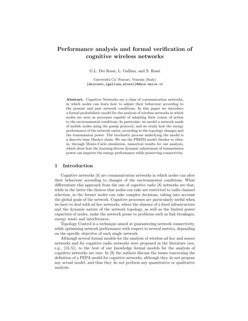
The results for a distance of 28.3m are shown in Figure 2.(a).We notice that, while with a fixed radius of 10 or 20m, the energy costs of

the communications critically increase, especially for small value of the gossipprobability psend, using cognitive processes, or a fixed radius of 15m, the per-formance is consistently improved. Since the curves for the variable radius andthe fixed radius 15m almost overlap, Table 3 reports the results in detail.

We analyse the average number of retransmissions, after the first one, thatthe sender node must perform to complete the communication with the receivernode, since it is useful to better understand the results of the previous reward

11

(a) Energy Costs

(b) Expected Number of Sender’s Retransmissions

Fig. 2: Distance between sender and receiver: 28,3 m

property verification. Figure 2.(b) shows some results for this kind of analysis.Notice that, by fixing the radius to the maximum value, on average the com-munication reaches the successful state after less than 1 retransmissions. As aninstance, the result for psend = 0.65 is 0.67567. Here the energy waste is givenby the high power employed for each forwarding, rather than by the numberof transmissions to reach the success. Again the curves for the Variable Ra-dius, and the Fixed Radius 15m are almost overlapping. This result lead us tothe conclusion that, with this particular network configuration, if the processescan dynamically choose their transmission radius, depending on the neighbours’positions, the average radius will be 15m.

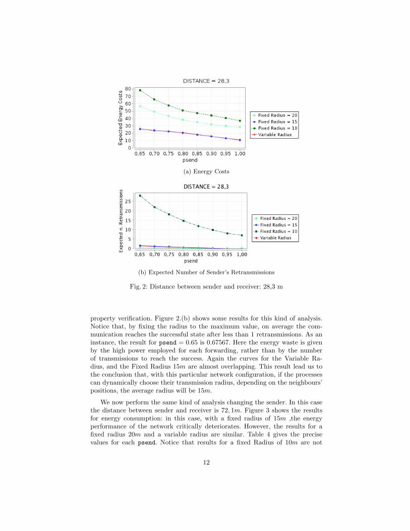
We now perform the same kind of analysis changing the sender. In this casethe distance between sender and receiver is 72, 1m. Figure 3 shows the resultsfor energy consumption: in this case, with a fixed radius of 15m ,the energyperformance of the network critically deteriorates. However, the results for afixed radius 20m and a variable radius are similar. Table 4 gives the precisevalues for each psend. Notice that results for a fixed Radius of 10m are not

12

(a) Energy Costs

(b) Expected Number of Sender’s Retransmissions

Fig. 3: Distance between sender and receiver: 72,1 m

reported: this is due to the fact taht the power needed for small values of psendis very high and this would have led to an unreadable graph.

Again the analysis of the number of retransmissions by the sender nodesis helpful to understand the behaviour of the network: the curves for a fixedradius and a variable radius are similar. For psend = 0.65 we have, on average,1.6834 retransmissions for the fixed radius network, and 2.519 for the cognitivenetworks, while for psend = 1.0 we have 0 on average for both the networkconfigurations), meaning that, for a larger distance a fixed radius 20m is close tothe ideal value of the transmission radius to guarantee the energy performanceoptimisation.

The results prove that, using a fixed radius, the performance of the networkstrictly depends on the relative positions of the sender and the receiver, whileusing a variable radius, we always get a power consumption that is closed to theminimum (that is closed to the fixed radius 15m in the first case, and to thefixed radius 20m in the second case).

13

Table 4: Results for Energy Costs, Distance = 71,2 m

VariableRadius

psend cost0.65 60.90900.7 50.613830.75 44.640670.8 40.11770.85 34.99500.9 32.87250.95 30.82921.0 28.6423

FixedRadius = 20

psend cost0.65 54.79330.7 48.952670.75 42.72870.8 38.39730.85 34.26730.9 32.10870.95 30.28071.0 28.1893

6 Conclusion

In this paper we have presented a probabilistic model for a class of cognitivenetworks in a wireless setting, in which nodes dynamically choose their trans-mission power, using data collected from the network itself. We have shown howthis model can be encoded in the PRISM language, allowing for the analysis ofits performances and for the verification of properties of its behaviour. Moreover,we have used that kind of analysis to compare the energy efficiency of those net-works with others based on different strategies, namely ones in which a statictransmission power is set. We have given some numerical results about this com-parison, and we have concluded that cognitive-networks-based strategies couldbe effective in the analysed setting.

Future works. As a further enhancement of our model, we plan to considermore sophisticated routing protocols, and different decision strategies as well.On the other hand, further simplifications of the model could lead to a fastersolution, even for models with a greater number of nodes. Moreover, the analysisof different kinds of rewards, such as latencies or throughputs, could, and should,be performed in order to better understand any possible advantage or drawbackof a power allocation strategy in wireless settings.

References

1. A.G. Dimakis, A.D. Sarwate, , and M.J. Wainwright. Geographic Gossip: EfficientAggregation for Sensor Networks. In Proc. of the 5th international conference onInformation processing in sensor networks, pages 69–76. ACM, 2006.

2. J. Scott Donald and Alec Yasinac. Dynamic probabilistic retransmission in ad hocnetworks. In Proc of the Int. Conference on Wireless Networks (ICWN04, pages158–164. CSREA Press, 2004.

3. A. Fehnker and P. Gao. Formal Verification and Simulation for Performance Anal-ysis for Probabilistic Broadcast Protocols. In Ad-Hoc, Mobile, and Wireless Net-

14

works, volume 4104 of Lecture Notes in Computer Science, pages 128–141. SpringerBerlin Heidelberg, 2006.

4. C. Fortuna and M. Mohorcic. Trends in the Development of Communication Net-works: Cognitive Networks. Computer Networks, 53(9):1354 – 1376, 2009.

5. E. Gelenbe and R. Lent. Power-aware ad hoc cognitive packet networks. Ad HocNetworks, 2(3):205 – 216, 2004.

6. Z.J. Haas, J.Y. Halpern, and L. Li. Gossip-based Ad Hoc Routing. IEEE/ACMTrans. Netw., 14(3):479–491, 2006.

7. H. Hansson and B. Jonsson. A logic for reasoning about time and reliability. FormalAspects of Computing, 6(5):512–535, 1994.

8. J. Mitola III. Cognitive Radio - An Integrated Agent Architecture for SoftwareDefined Radio. PhD thesis, Royal Institute of Technology, Stockholm, Sweden,2000.

9. L. Guo J. Wang and G. Zhao. Study on Formal Modeling and Analysis MethodOriented Cognitive Network. In Computational Intelligence and Design (ISCID),2012 Fifth International Symposium on, volume 2, pages 402–405, 2012.

10. M. Z. Kwiatkowska, G. Norman, and D. Parker. Prism 4.0: Verification of prob-abilistic real-time systems. In Ganesh Gopalakrishnan and Shaz Qadeer, editors,CAV, volume 6806 of Lecture Notes in Computer Science, pages 585–591. Springer,2011.

11. G. Norman M. Kwiatkowska and D. Parker. Advances and Challenges of Proba-bilistic Model Checking. In 48th Annual Allerton Conference on Communication,Control, and Computing, pages 1691–1698. IEEE, 2010.

12. T. V. Madhav and N.V.S.N. Sarma. Maximizing Network Lifetime through VaryingTransmission Radii with Energy Efficient Cluster Routing Algorithm in WirelessSensor Networks. International Journal of Information and Electronics Engineer-ing, 2(2):205–209, 2012.

13. T. Mahmoodi. Energy-aware routing in the cognitive packet network. PerformanceEvaluation, 68(4):338 – 346, 2011.

14. P. Santi. Topology Control in Wireless Ad Hoc and Sensor Networks. ACMComputing Surveys (CSUR), 37(2):164–194, 2005.

15. W. J. Stewart. Probability, Markov Chains, Queues, and Simulation. PrincetonUniversity Press, UK, 2009.

16. O. Younis and S. Fahmy. HEED: A Hybrid, Energy-Efficient, Distributed Cluster-ing Approach for Ad Hoc Sensor Networks. Mobile Computing, IEEE Transactionson, 3(4):366–379, 2004.

17. Hongqiang Zhai and Yuguang Fang. Physical carrier sensing and spatial reuse inmultirate and multihop wireless ad hoc networks. In Proc. of INFOCOM 2006.25th IEEE International Conference on Computer Communications, pages 1–12,2006.

15