percolation of ions through structured coatings - ucl.ac.ukucapikr/projects/john nutter final...

1

Percolation of ions through structured

coatings

Using Finite Element Analysis software to model the behaviour of current through an

anisotropic material.

John Nutter

University College London

Department of Physics and Astronomy

30th March 2012

First Supervisor: Prof Ian Robinson

Second Supervisor: Dr Graeme Morrison

2

Contents

Acknowledgements 4

Introduction 4

Background 5

Corrosion 5

o Pourbaix diagrams 6

Electrochemistry 7

o Calculating the potential of a typical electrochemical cell 7

Formation of rust 8

Passivity 9

o Effect of chlorides 9

Corrosion processes 10

o Uniform corrosion 10

o Galvanic corrosion 10

o Pitting and crevice corrosion 10

o Pitting 11

o Crevice corrosion 13

Anti-corrosive coatings 13

o Factors affecting coating effectiveness 14

Diffusion 16

o Anisotropy 16

Modelling an ideal structure 17

COMSOL Multiphysics® 17

Building the model 18

Finite Element Analysis – Meshing 19

Conjugate Directions Method 21

o Conjugate Gradients 23

Results & Discussion 23

o Time-Dependent Heat Transfer 27

Modelling the real material 28

Imaging Techniques 28

3

o 3-View 28

o Ptychography 30

Simulating the Real Material 30

Results & Discussion 31

Conclusion 35

Appendices 37

References 38

4

Acknowledgements

I would like to express my thanks to Professor Ian Robinson for acting as my supervisor

over the course of this project. In addition, I would also like to thank Dr Gang Xiong for his

help with the COMSOL® modelling and Bo Chen for providing the 3-View and

ptychography images used in this project.

Introduction

It is frequently asserted that the total costs associated with the effects and prevention of

corrosion in the United States and other industrialised countries is around 4% of the gross

national product[1][2]. In the marine environment, failure to protect vessels from corrosion

can have spectacular consequences such as when the oil tanker Erika broke in two in

1999 as a ““direct consequence of the serious rust corrosion” caused by “insufficient

maintenance of the ship””[3] and spilt some ten million litres of oil off the coast of

Brittany[4].

Due to the corrosive nature of the marine environment caused by the relatively high

salinity of seawater it is necessary for the hulls, ballast tanks etc. of the predominantly

steel ships in use today to have sufficient protection from this environment. This can be

done in a number of ways including the use of sacrificial anodes, but the most common

technique is to use paints or coatings on areas likely to be affected. An effective anti-

corrosive coating or paint acts as a barrier to prevent the water, oxygen and salt ions from

adsorbing onto the metal substrate. The property which defines the effectiveness of the

coating is its permeability, which is determined by a number of factors including the

pigment to binder ratio and the shape of those pigments[5].

The effect of shape and concentration of pigments in the coating can be modelled using

finite-element analysis software packages, such as COMSOL Multiphysics®. This has a

number of advantages over more experimental techniques such as the Payne Cup[6]

since the software has greater potential for understanding the behaviour of current or heat

5

flow through the material itself.

The results of these simulations can then be compared with reality by modelling the flow of

current through an image of an actual material used as an anti-corrosive coating. These

images were obtained using two relatively new techniques Ptychography, an X-ray

technique for retrieving phase information, and 3View, a serial sectioning technique which

uses scanning electron microscopy.

Background

Corrosion

The corrosion of metals is an electrochemical process caused by the existence of

thermodynamically stable oxidation states for a given metallic species. The stability of the

various oxidation states for an element can be represented using a Frost Diagram (figure

1)

Figure 1: Frost Diagram for Manganese [8]

Many, though not all, metals naturally occur as oxides, sulphides, chlorides or carbonates.

When these metals are extracted from their ores they are reduced to an oxidation state of

zero. Since this oxidation state is less stable, there has been a gain of energy, so when the

metal comes into contact with oxygen, sulphur or a similar chemical species there will be a

6

favourable reaction resulting in a lowering of the free energy and a return to the stable

oxidation state[9]. Therefore metals will tend to revert to these compounds.

In practice, this means that metallic structures, with the exception of noble metals such as

gold, that are exposed to the elements will gradually corrode.

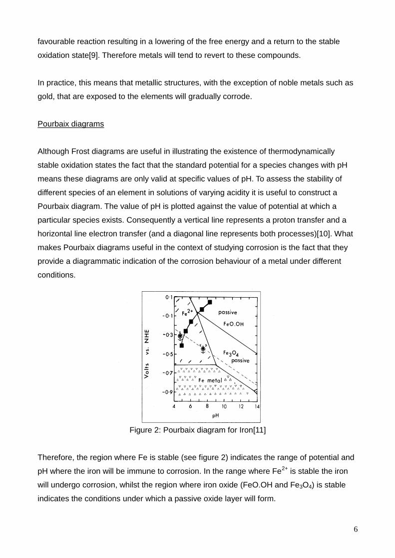
Pourbaix diagrams

Although Frost diagrams are useful in illustrating the existence of thermodynamically

stable oxidation states the fact that the standard potential for a species changes with pH

means these diagrams are only valid at specific values of pH. To assess the stability of

different species of an element in solutions of varying acidity it is useful to construct a

Pourbaix diagram. The value of pH is plotted against the value of potential at which a

particular species exists. Consequently a vertical line represents a proton transfer and a

horizontal line electron transfer (and a diagonal line represents both processes)[10]. What

makes Pourbaix diagrams useful in the context of studying corrosion is the fact that they

provide a diagrammatic indication of the corrosion behaviour of a metal under different

conditions.

Figure 2: Pourbaix diagram for Iron[11]

Therefore, the region where Fe is stable (see figure 2) indicates the range of potential and

pH where the iron will be immune to corrosion. In the range where Fe2+ is stable the iron

will undergo corrosion, whilst the region where iron oxide (FeO.OH and Fe3O4) is stable

indicates the conditions under which a passive oxide layer will form.

7

Electrochemistry

The corrosion of metals, such as Iron, and their alloys is an electrochemical process in

which the metal is oxidised into a more stable oxidation state whilst water, oxygen or other

species are reduced. Example half equations for this process for Iron (in a neutral or

alkaline solution) are:

Fe → Fe2+ + 2e-

O2 + 2H2O + 4e- → 4 -OH

These simultaneous reactions result in the formation of an electrochemical cell as

illustrated in figure 3 below, with the oxidation taking place at the anode and reduction at

the cathode.

Figure 3: An electrochemical cell formed by the corrosion of Iron in water[12]

This electrochemical cell has a potential, Ecell, which is determined by the potentials of the

reactions which occur at the anode and the cathode.

Calculating the potential of a typical electrochemical cell

For a typical electrochemical cell formed, in this example, by the connection of copper and

zinc by an ionic conductor[13], the standard cell potential, Ecell, can be calculated using the

following half equations:

Cu2+(aq) + 2e- → Cu(s) E(Cu2+, Cu) = +0.34V

Zn2+(aq) + 2e- → Zn(s) E(Zn2+, Zn) = -0.76V

8

Where E(Cu2+, Cu) and E(Zn2+, Zn) are the standard electrode potentials for copper and

zinc respectively. Copper's more positive potential means that it will be reduced in the

reaction and zinc's more negative potential indicates that it will be oxidised, thus the

reaction that takes place is:

Zn(s) + Cu2+(aq) → Zn2+

(aq) + Cu(s)

The cell potential is therefore given by:

Ecell = E(Cu2+, Cu) - E(Zn2+, Zn)

Ecell = 0.34 - -0.76

E = +1.1V

However, the electrochemical cell formed during the corrosion of iron does not exist in

standard conditions and therefore calculating the cell potential becomes more difficult.

According to Satsri et al[14]:

“In most of the corrosion reactions, the potential values... are not applicable because of the

presence of a film on the metal surface, and the change in potential because the activity of

the metal ions is less than unity”

Formation of rust

The metal ions then react with the hydroxyl ions forming metallic hydroxides. Again using

Iron as an example:

Fe2+ + 2 -OH → Fe(OH)2

Further reaction with oxygen produces a hydrated metallic oxide compound, or rust:

2Fe(OH)2 + O2 → Fe2O3.H2O

A number of factors influence the rate at which this occurs such as temperature, oxygen

concentration and pH. One of the most important, especially for the purposes of this

project, is the concentration of dissolved ions in the seawater. This affects the rate at which

metals corrode in two significant ways. Firstly the presence of dissolved salt ions increases

9

the conductivity of the electrolytic solution, in this case water. Secondly the ions break

down the passivating layer of metal oxide which forms on the surface of the metal.

Passivity

A surface is passive if there is significant resistance to corrosion despite the fact that the

reaction may be thermodynamically favourable, due to the existence of an oxide layer at

the metal-electrolyte interface[7]. For example, the corrosion of Aluminium would be

expected to proceed, if only the thermodynamic favourability of the reaction was taken into

consideration, at a far greater rate than is actually the case due to the formation of a dense

Al2O3 layer on the surface of the metal[29].

At the most basic level the oxide layer reduces the rate at which metallic cations can

diffuse into solution, resulting in a build-up of positively charged ions at the site where

corrosion is taking place. This in turn reduces the rate at which the metal is ionised and

therefore lowers the rate at which the metal corrodes[15].

Effect of Chlorides

According to Ulick R. Evans it is “difficult to produce, or even to maintain, passivity in the

presence of chlorides”[16]. The main reason suggested for this is that the Chloride ions

displace H2O molecules which adsorb to the metal surface at the anode[15]. This occurs

because the polar water molecules have only a partial negative charge compared to a full

negative charge on the ions. As a consequence of this the initial corrosion product is

ferrous chloride (FeCl2) rather than Iron oxide[17]. Due to its higher solubility compared

with the oxide, the FeCl2 molecules are transported a greater distance from the surface

before undergoing hydrolysis and being precipitated[16].

10

Corrosion Processes

There are a number of processes through which corrosion takes place. Some of the most

relevant are outlined below.

Uniform Corrosion

This is the most commonly encountered form of corrosion and is generally responsible for

the greatest loss in the metal. In order for it to occur the entire surface must be exposed to

a corrosive environment which causes a more or less uniform dissolution of the metal from

the surface of a corroding structure[18]. Figure 4 shows a schematic diagram of this

process.

Figure 4: Metal lost due to uniform corrosion.

Galvanic Corrosion

Galvanic corrosion is similar to the general electrochemical corrosion outlined above but

instead takes place in a galvanic cell where two different metals are oxidised or reduced.

Galvanic cells occur where two different metals or alloys are adjacent and coupled by an

electrolyte[18][19]. This means that one alloy forms the anode and the other the cathode.

Pitting and Crevice Corrosion

Pitting and Crevice corrosion are two forms of highly localised corrosion that proceed

through similar mechanisms[20]. These localised processes present a far greater problem

than the reasonably predictable uniform corrosion of a surface, firstly because the

11

formation of pits in a metal is more difficult to predict[15] (particularly in small scale

laboratory experiments[21]) and secondly because it can lead to the failure of a structure

with only a relatively small weight of the metal being lost to corrosion. These pits can also

give rise to other forms of corrosion such as stress corrosion cracking and fatigue

corrosion.

Pitting

Pitting is particularly associated with the breakdown of the passive oxide layers on the

surface of a metal or alloy[22]. Pits begin at defects in the passive film since these points

are anodic relative to the rest of the film.

Since the localisation reduces the ability of ions to be transported away from the site the

concentration of metal cations produced by the corrosion process increases, as a

consequence negatively charged ions dissolved in the solution are attracted to the region

reacting with the metal ions.

M+ + Cl- → MCl

The Metallic Chlorides then undergo hydrolysis producing Metallic Hydroxides and

Hydrochloric acid:

MCl + H2O → MOH + HCl

This hydrochloric acid decreases the pH of the solution in the pit or crevice making it more

corrosive, whilst the Chloride ions from the acid (HCl → H+ + Cl-) go on to react with further

metal ions. Thus the process is an autocatalytic one.

Thermodynamically, pitting is controlled by a number of factors. When the structure first

comes into contact with corrosive ions there is an 'induction time', t, before pits nucleate on

the surface[22]. The length of this induction period depends on the concentration of

corrosive ions (equation 1) and the potential of the cell.

12

Equation 1:

T = C-n

where n depends on the type of ion (for Cl- n is between 2.5 & 4.5[15])

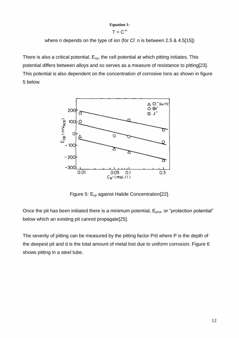
There is also a critical potential, Ecp, the cell potential at which pitting initiates. This

potential differs between alloys and so serves as a measure of resistance to pitting[23].

This potential is also dependent on the concentration of corrosive Ions as shown in figure

5 below.

Figure 5: Ecp against Halide Concentration[22].

Once the pit has been initiated there is a minimum potential, Eprot, or “protection potential”

below which an existing pit cannot propagate[25].

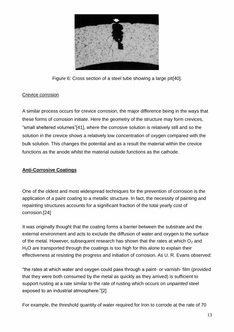
The severity of pitting can be measured by the pitting factor P/d where P is the depth of

the deepest pit and d is the total amount of metal lost due to uniform corrosion. Figure 6

shows pitting in a steel tube.

13

Figure 6: Cross section of a steel tube showing a large pit[40].

Crevice corrosion

A similar process occurs for crevice corrosion, the major difference being in the ways that

these forms of corrosion initiate. Here the geometry of the structure may form crevices,

“small sheltered volumes”[41], where the corrosive solution is relatively still and so the

solution in the crevice shows a relatively low concentration of oxygen compared with the

bulk solution. This changes the potential and as a result the material within the crevice

functions as the anode whilst the material outside functions as the cathode.

Anti-Corrosive Coatings

One of the oldest and most widespread techniques for the prevention of corrosion is the

application of a paint coating to a metallic structure. In fact, the necessity of painting and

repainting structures accounts for a significant fraction of the total yearly cost of

corrosion.[24]

It was originally thought that the coating forms a barrier between the substrate and the

external environment and acts to exclude the diffusion of water and oxygen to the surface

of the metal. However, subsequent research has shown that the rates at which O2 and

H2O are transported through the coatings is too high for this alone to explain their

effectiveness at resisting the progress and initiation of corrosion. As U. R. Evans observed:

“the rates at which water and oxygen could pass through a paint- or varnish- film (provided

that they were both consumed by the metal as quickly as they arrived) is sufficient to

support rusting at a rate similar to the rate of rusting which occurs on unpainted steel

exposed to an industrial atmosphere.”[2]

For example, the threshold quantity of water required for Iron to corrode at the rate of 70

14

mg/cm2/year is 0.93 grams/m2/day, an amount which is far lower than quantity of water

which does, in fact, pass through many coatings. For instance ~30 grams/m2/day of water

is transmitted through coal tar epoxy[27].

Factors affecting coating effectiveness

A number of factors are necessary for a paint to function as an effective anticorrosive

coating, as figure 7 shows.

Figure 7: Some of the desired properties of an effective anticorrosive coating[28].

First, it is necessary for the paint to have good adhesive properties. Good adhesion to the

substrates will prevent the formation of an electrolytic layer which will connect the anodic

and cathodic sites of the electrochemical cell formed when a metal undergoes corrosion.

In addition, since coatings are not impervious to the penetration of water, oxygen and other

chemical species this adhesion will prevent the coating from failing more generally due

blistering, one cause of which is the condensation of moisture at points of poor

adhesion[26].

Secondly, the chemistry of the pigments in the paint and of the paint itself greatly

contributes to its anticorrosive properties. For instance, the Al2O3 layer on the surface of

Aluminium pigments is thought to reduce cathodic disbonding of coatings by reacting with -

OH ions[30]. Similarly Zinc dust pigments form corrosion products which block the pores in

the coating and hinder further diffusion through it[31].

Thirdly, it is desirable that the paint does not degrade in UV light, since this would lower its

effective lifetime.

15

However, for the purposes of this project it is maintaining a low permeability to ionic

species that is of particular interest. The rate at which corrosion progresses in seawater is

high compared to that seen in freshwater and other environments due to the presence of

high concentrations of dissolved ions such as Na+, Cl- and S2-. These ions serve to

increase the conductivity of the water and so allow the reactions between the metal and

hydroxide ions to take place much more rapidly, a high resistance to ionic mobility greatly

reduces this.

Resistance to ionic mobility can be achieved either through the properties of the binder or

through the addition of barrier pigments. The unadulterated binder may have a low

permeability due to extensive cross linking as is the case in many epoxy resins.

Alternatively, the presence of carboxylic acid (-COOH) and other ionisable groups in the

binder may impede the movement of negatively charged ions[32].

The alternative is to add barrier pigments which will lengthen the diffusional pathways for

the diffusing species. The most common types of barrier pigment are micaceous Iron

Oxide, as well as glass and Aluminium flakes; these lamellar pigments are preferred since

they offer the greatest lengthening of the diffusional pathways, which tend to align parallel

to the substrate as a result of the shrinking of the binder due to solvent evaporation.

As the concentration of pigments increases the permeability is decreased. However, there

exists a Critical Pigment Volume Concentration (CPVC) which represents the point at

which any further increase in the concentration of the pigment will fundamentally change

the properties of the paint. Beyond this CPVC there is an insufficient quantity of binder to

keep the coating together. One consequence of this is that as the CPVC is approached the

binder does not necessarily fill all of the gaps between the pigments and so the

permeability increases[5], lowering the effectiveness of the coating.

16

Diffusion

Since the quantity of ions dissolved in seawater is sufficiently large compared to the

quantity which will diffuse through the marine coating, then it is reasonable to assume that

the concentration of the diffusing species remains constant. Therefore, the diffusion

process can be described by Fick's First Law (in one dimension):

Equation 2:

JN = - D dC/dx

Where JN is the number of atoms passing through a unit area in unit time, D is the

diffusivity and dC/dx is the concentration gradient.

This equation is formally equivalent to the equations which describe the transport of heat

and electric charge, Fourier's Law and Ohm's law respectively, which are given below:

Equation 3: Fourier’s Law

q = -k ΔT

Where q is the heat flux, k is the thermal conductivity and ΔT the temperature gradient.

Equation 4: Ohm’s Law

J = σE

Where J is the current density, σ is the conductivity and E is the applied electric field. For a

uniform electric field, E = -V/d.

Consequently, the behaviour of diffusing ions can be described using Fourier's Law and

Ohm's Law. However, this will be subject to certain limitations; for instance, the rate at

which a species diffuses through a material is far lower than the rate at which heat is

transferred through it.

Anisotropy

The presence of shaped pigments in the paint will introduce an anisotropic property to the

diffusivity and conductivity of the material. In three dimensions Fick's First Law

becomes[33]:

Equation 5:

J N= −D∇C

17

Which for an anisotropic material can be rewritten as[34]:

Equations 6-8:

J1 = -D1 dC/dx1

J2 = -D2 dC/dx2

J3 = -D3 dC/dx3

with D1, D2, D3 being related to D by:

Similarly it will be possible to decompose conductivity into σ1, σ2 and σ3. The Aluminium

and Mica flakes will tend to align themselves in the xy plane, this means that they will

present a lower conductivity for a potential difference applied along the z direction

compared to in the x or y direction. Therefore the Anisotropy, ε, of the material can be

expressed as a ratio of the conductivities:

Equation 9:

ε = σz / σy

Modelling an Ideal Structure

COMSOL Multiphysics®

COMSOL Multiphysics® is a Finite Element Analysis software package. It includes

numerous modules which allow multiple physical situations to be simulated. The AC/DC

module provides an interface for the modelling of electromagnetism, the Heat Transfer

module for the modelling of heat transfer and so on. These modules can be used

separately or in combination to simulate 'multiphysics' models (such as Joule heating).

Although it provides a graphical interface it is also possible to use COMSOL in conjunction

with MATLAB®.

18

Building the Model

The first step was to create an ideal version of the material in order to model the behaviour

of current in a simple scenario as well as to ascertain how the anisotropy of the material

changes with changing 'pigment' size and concentration. The model contained a number of

simplifications. Firstly, the pigments were all of the same size and material. Secondly, all of

the pigments were aligned along the xy plane. As previously noted the shrinking that the

binder undergoes due to solvent evaporation causes lamellar pigments to align parallel to

the surface, however, they do not align perfectly. By placing all the pigments in this plane

the anisotropy of the material for a given size and concentration is maximised. Thirdly, the

pigments were arranged in a regular 3x3 array with ABCD stacking between layers. This

was necessary to ensure that there was no short circuit through the array.

Below (figure 8) is an image of the initial geometry. The structures representing the

pigments are cylinders of radius 6 microns with a height of 0.3 microns.

Figure 8: Creating the initial geometry

This was achieved by first creating a cube of 50x50x50 microns and then creating the

cylinders 1-4. These were then used to create an array consisting of a series of 3x3 layers

5 microns apart, with 8 layers in total. A Boolean difference operation was then performed

to remove the volume represented by this array of cylinders, leaving a cube with an array

of cylindrical holes inside.

It is possible to perform the simulation using these holes to represent the pigment (since

19

no current can flow across them), however, because the pigments do not completely

prevent the flow of ions, it was necessary to recreate the array using another four cylinders

(cylinders 5-8) in the same positions as before.

The next step was to define the materials. The cylinders were grouped together as a single

material which was assigned a conductivity of 1x10-10 S/m. Whilst the cube, which

represents the epoxy, was assigned a conductivity of 1x1010 S/m.

Next, the boundary conditions were assigned. The edges of the structure are insulating by

default and a potential difference of 10V was applied across the z axis. This was achieved

by simply selecting the desired face and setting Vo to 10V (see figure 9) and then making

the opposite face grounded.

Figure 9: Electric Potential

Finally the structure was meshed.

Finite Element Analysis - Meshing

Finite Element Analysis is a numerical method for providing approximate solutions to

problems that cannot be solved exactly due to their complexity.

Since a continuous structure can have an infinite number of degrees of freedom, the

structure is broken up into a number of discrete elements (in this case the elements were

tetrahedral). Whilst this limits the number of degrees of freedom it introduces a

20

discretisation error which increases as the size of the elements increases, meaning there

is a trade-off between accuracy and complexity of the model.

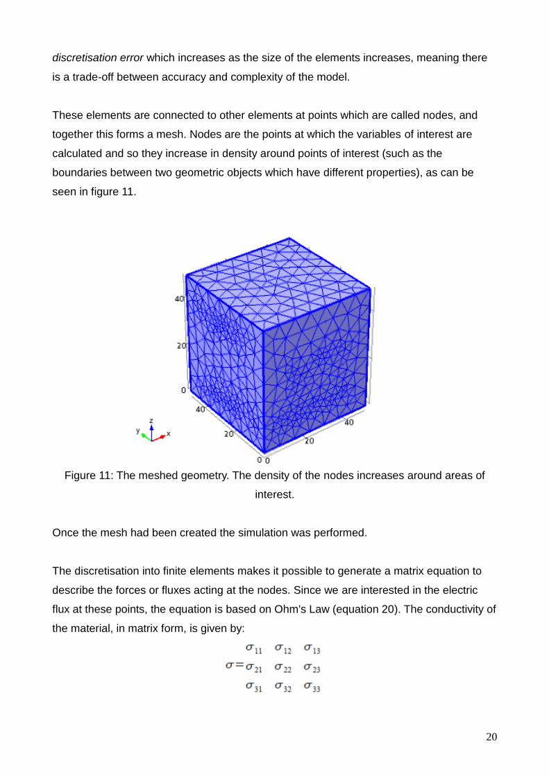
These elements are connected to other elements at points which are called nodes, and

together this forms a mesh. Nodes are the points at which the variables of interest are

calculated and so they increase in density around points of interest (such as the

boundaries between two geometric objects which have different properties), as can be

seen in figure 11.

Figure 11: The meshed geometry. The density of the nodes increases around areas of

interest.

Once the mesh had been created the simulation was performed.

The discretisation into finite elements makes it possible to generate a matrix equation to

describe the forces or fluxes acting at the nodes. Since we are interested in the electric

flux at these points, the equation is based on Ohm's Law (equation 20). The conductivity of

the material, in matrix form, is given by:

21

However, for an anisotropic material, only the diagonal elements are non-zero. Thus the

matrix becomes:

The algorithm used to solve this problem is known as the Conjugate Gradients method.

This is an iterative method which solves a system of n linear equations of the form Ax = b

where A is an invertible, symmetric matrix[35], and x and b are column vectors.

Conjugate Directions Method

In fact, the conjugate gradient method is a special case of the method of conjugate

directions[35], which is described below.

The actual solution of Ax = b is where x = h (i.e. Ah = b). If h is estimated as x then it is

possible to define a residual, r, which represents the distance from the correct value of

b[36]:

Equation 10:

ri = b – Axi

Whilst the difference from h is given by the error vector, e:

Equation 11:

ei = h – xi

The conjugate gradient method begins with an estimate of h, xo, and determines n new

estimates (x1, x2,... xn) in which xi+1 is closer to h than xi[35] which reduces both e and r.

The conjugate directions method uses a set of search directions do,d1 ... dn-1 which are A-

orthogonal, that is:

Equation 12:

diTAdj = 0

22

The method begins with an estimate of h, xo, and a search direction, do, followed by a

calculation of the residual. The next step is to estimate x1. Since the direction of the search

has already been defined x1 will be estimated at:

Equation 13:

x1 = xo + αodo

Where αo describes the distance along do x1 will be located and is decided by a desire to

minimise the error vector e1. Since, the error vector will have its minimum value at the

point that do is closest to the solution, h, then the error vector will be A-orthogonal, or A-

conjugate, to do so:

Equation 14:

doTAe1 = 0

and since

Equation 15:

e1 = eo + αodo

then equation 14 becomes

Equation 16:

doTA(eo + αodo) = 0

which rearranges to:

Equation 17:

and since Aeo is equal to ro (from equations 10 and 11):

Equation 18:

finally enabling x1 (equation 13) to be calculated.

23

Conjugate Gradients

What differentiates conjugate gradients from other cases of the more general conjugate

direction method is the way in which the search directions are generated[35]. For

conjugate gradients the new search direction is given by

Equation 19:

d1 = r1 + β1do

where β1 is given by

Equation 20:

Results & Discussion

The simulation was performed for cylinders of varying radius and varying distance

between the layers. A ratio of Jz/Jy was calculated to get a value for the anisotropy, ε.

These values are reproduced in table 1 below.

Table 1

Radius, Spacing (microns) Ε = Jz/Jy = σz/σy

1 R = 3, d = 10 0.904

2 R = 3, d = 5 0.830

3 R = 6, d = 10 0.832

4 R = 6, d = 5 0.723

5 R = 12, d = 5 0.562

6 R = 12, d = 2.5 0.405

Relative Errors 0.005 – 0.009

This shows that the anisotropy increases as the size and concentration of the cylindrical

pigments increases. This is analogous to an increase in the path length of a diffusing

species, as they must move around the barrier pigments.

24

This can be seen in figure 12 below which shows a slice through the material with a

potential difference applied across the z axis.

Figure 12: Slice in the yz plane showing the z component of current density

Figure 12 shows the z component of the current density. The black lines are the cylinders

(the large lines where the slice is through the centre of the cylinder and the smaller lines

where the slice is closer to the edge), the blue regions represent areas of high current

density and the red regions areas of lower current density.

The high density regions occur around the edges of the cylinders and the low density

regions around the centre. However this is not the full picture, as can be seen from figure

13.

25

Figure 13: Slice in the yz plane showing the y component of current density

Figure 13 shows the same slice as figure 12 but in this case with the y component of the

current density. The red/yellow regions show the y component moving in the positive y

direction, and the blue in the negative y direction. This shows that the current is flowing

around the cylinders exactly as would be expected.

Contrast this with figures 14 & 15 which show the same slices but this time with current

applied along the y direction.

26

Figure 14: Slice in yz plane showing y component of current density

Figure 15: Slice in yz plane showing z component of current density

27

As can be seen from the two figures above there is far less contrast in the current

densities, apart from the regions around the edges of the cylinders the current is relatively

uniform, indicating that the current travels along a much more torturous path than along

the z axis than when the voltage is applied along the y axis.

It is also worth noting that similar path lengths formed from different cylinder sizes give

similar anisotropy ratios. For example the anisotropy for simulations 2 and 3 in table 2 are

0.830 and 0.832 respectively. The first has 8 layers of cylinders with a radius of 3 microns

and the second 4 layers with a radius of 6 microns. It is intuitively obvious that these would

present a similar increase in path length. Graph 1 shows the anisotropy, ε, for each

simulation.

Graph 1: anisotropy against simulation number

In addition, the simulations were also performed with a lower conductivity of the epoxy

(500 S/m) with similar results.

Time-Dependent Heat Transfer

The original structure was also modelled using time-dependent heat transfer. Ideally this

would have been carried out on the images of the real material but due to insufficient

28

memory on the computer this was not possible, however, it does show that the same

behaviour is found for both heat flux and current density. The Isotherms in figure 16 show

the effect of the poorly conducting cylinders on the transfer of heat through the structure.

Figure 16: Isotherms at t=18.4

Modelling the real material

Imaging Techniques

The images of the real material were obtained using two techniques: 3-View and

Ptychography.

3-View

3-View is a Scanning Electron Microscopy technique which uses an automated diamond

knife to cut slices (which can be as small as 40nm thick) from a sample. The surface of the

sample is imaged before the specimen is cut, revealing a new surface which is then

imaged. This process is then repeated to produce a series of images which can be stacked

to form a 3D image of the structure. This represents an improvement on previous

techniques where the specimen needed to be sliced using a microtome before being

imaged.

29

Scanning Electron Microscopy

Scanning Electron Microscopy (SEM) uses a focused electron beam from a heated

filament (such as tungsten) in order to image a sample. The electron beam interacts with

the atoms within a region known as the interaction volume, and the size of this volume

depends on the electron energy and target density[37]. The interaction of interest in this

case is the backscattering of electrons since it not only allows the surface topography to

be imaged, but by measuring the proportion of electrons backscattered different materials

on the surface can be contrasted:

Equation 21:

Where Ibackscattered is the backscattered electron current and Iincident is the incident electron

current.

This is because the proportion of electrons which are backscattered depends on the

atomic number, Z, as is shown in figure 18.

Figure 18: backscattered electron coefficient against atomic number[43].

For a flat surface it is possible to differentiate between two areas in which the atomic

number differs by only 1[37].

30

Ptychography

Ptychography (from the Greek for ‘fold’) is a phase retrieval algorithm invented by Walter

Hoppe[38]. When the diffraction patterns from coherent X-rays are collected only the

intensities are recorded and the phases are lost. These phases need to be retrieved in

order to reconstruct the image.

To this end a sequence of far field diffraction images are taken, as can be seen in figure

19, using a localised moving probe[44]. Between each image the probe is moved a

distance smaller than the beam diameter resulting in the imaging of a series of overlapping

regions.

Figure 19: Schematic showing the setup for ptychography[39]

These regions make it possible to retrieve the phase information and thereby reconstruct

the image.

Simulating the real material

The simulations were carried out on four images, two obtained using 3-View and two

obtained using ptychography, the images were NASTRAN mesh (.bdf) files which could be

imported into COMSOL multiphysics® and used as a predefined mesh.

The pigments were then assigned a conductivity of 1x10-10 S/m and the epoxy was

assigned a conductivity of 500 S/m (see figure 20) and a potential difference was applied

across the z axis (in the 3-View case) or the x axis (for ptychography) in the same way as

for the previous simulations on the ideal structure.

31

Figure 20: An image obtained using 3-View. The pigments are shown on the left and the

epoxy on the right

Results & Discussion

The ratios for the anisotropy can be seen in table 2.

Table 2

Technique E Relative Error

1 3-View 0.555 0.010

2 3-View 0.516 0.0079

3 Ptychography 0.358 0.0084

4 Ptychography 0.126 0.0074

In these cases it was important to give some consideration to the direction in which the

potential difference was applied. Unlike the ideal structures modelled initially these images

had pigments which extended to the sides of the structure and had been cut off.

Consequently if the 10V potential was applied along a face which had a large pigment at

the surface the current was effectively blocked off. This occurred for the second 3-View

simulation where much of the current had been blocked for nearly half of the structure, as

can be seen below in figure 21.

32

Figure 21: Slice in the yz plane showing the x component of current density, with a much

lower current density on the right side of the image.

As a consequence of this a value for ε nearly half of that quoted in table 3 (which was

calculated using a potential difference applied in the opposite direction) was calculated.

A particularly useful way to visualise the results was to create a 'streamline plot' which

produces a set of plots which are tangent to the vector field. These plots can be seen for

simulation 3 in figures 22 & 23 below.

33

Figure 22: zx plane view of the streamline plot (potential difference along the z axis)

Figure 23: xy plane view of the streamline plot (potential difference along the y axis)

34

These streamline plots show, even more clearly than the current density plots, how the

current behaves in the material. When the potential difference is applied along the x-axis it

is clear that the vector field is far more torturous than for is the case when the potential

difference is applied along the y-axis. In fact, figure 22 is particularly useful because it

contains a large flake in the middle of the image around which the current flows.

Of the two imaging techniques the ptychography showed greater anisotropy. This may be

due to the fact that the images were larger (a thickness of ~12 microns against ~6

microns) meaning that it contained whole or nearly whole aluminium flakes, resulting in a

lower conductivity along the x axis. In contrast the 3-View images only included fragments

of the large aluminium flakes. Furthermore, this may also be the reason why the two

simulations on images obtained using 3-View demonstrated closer agreement. Although

some variation is to be expected between different samples it can be seen by comparing

figure 24 with figure 22 that the reason why the second ratio was approximately a third of

the first was because the former contained two large flakes rather than only one.

Figure 24: Streamline current density plot for simulation 4 showing two large flakes

35

Conclusion

It has been shown that it is possible to use Finite-element analysis software (in this case

COMSOL Multiphysics®) to model the behaviour of current in both an ideal structure and in

the real material and, furthermore, that this behaviour is similar to that proposed in the

literature for the behaviour of diffusing species in coatings containing barrier pigments

(Compare figure 25 below with figure 24 or 22).

Figure 25: The lengthening of diffusion pathways[42]

The difference between the anisotropy obtained from the 3-View and ptychography images

shows that it is desirable for a large sample to be used since this will make it possible to

account for the effects of large flakes (or other structures) within the material. Furthermore,

during its actual application the thickness of the coating will be greater than the thickness

of the sample. From this point of view, depending on limitations of the sample size, it may

be more desirable to use ptychography to obtain the images to be simulated.

Apart from this the power of the computer proved to be a major limitation, particularly once

simulations of the real material had begun due to an increased number of mesh elements

(millions as opposed to hundreds of thousands of elements in the ideal structure). Not only

did this greatly increase the time taken to perform the simulations but also prevented other

COMSOL® modules from being used. For instance, Time-dependent heat transfer could

not be used on the imaged structure due to insufficient memory. However, it could be

36

useful to perform this simulation since it could provide information about the time taken for

a chemical species to diffuse through the material.

Finally, it is important to note that the simulation will only be appropriate for those materials

where diffusion through them obeys Fick's Laws.

37

Appendix

For the simulations of the ideal structure the material is a cube and so the area and length

of the material are the same along each axis. Consequently the ratio between

conductivities could be found by simply dividing Jz by Jy. However, the real material was

not cubic and so the fluxes needed to be multiplied by the length of the principle current

axes since

Jz / Jy = Iz/Az . Ay/Iy

= Ay . Ry / Az . Rz

R = ρl/A

so

Jz / Jy = ρy . Ly / ρz . Lz

Therefore

(Jz / Jy).(Lz/Ly) = ρy / ρz = σz / σy = ε

38

References

1. Parkins, R.N. Corrosion Processes, Applied Science Publishers: Barking, England

(1982) p. v

2. http://www.nace.org/content.cfm?parentid=1011&currentID=1045 (accessed

27/1/12)

3. http://www.english.rfi.fr/environment/20100330-total-loses-erika-oil-spill-appeal

(accessed 27/1/12)

4. http://news.bbc.co.uk/1/hi/world/europe/7192085.stm (accessed 27/1/12)

5. Weldon, D.G. Failure Analysis of Paints and Coatings, John Wiley & Sons:

Chicester, England (2001) p. 20

6. Payne, H.F.; Gardner, WM.H. Permeability of Varnish Films Relative Effect of

Structure and Other Factors, Industrial and Engineering Chemistry, 29(8): 893-898 (1937)

7. De Castro, M.A.C.; Wilde, B.E. The Corrosion and Passivation of Iron in the

Presence of Halide Ions in Aqueous Solution, Corrosion Science, 19: 923-936 (1979)

8. http://www.wou.edu/las/physci/ch462/redox.htm (accessed 10/3/12)

9. Evans, U.R. The Corrosion and Oxidation of Metals, Edward Arnold: London,

England (1960) p. 15

10. Atkins, P.; Overton, T.; Rourke, J.; Weller, M.; Armstrong, F. Inorganic Chemistry

(Fifth Edition), Oxford University Press: Oxford, England (2010) p. 168

11. Macleod, I.D. The application of corrosion science to the management of maritime

archaeological sites, Bulletin of the Australian Institute for Maritime Archaeology, 13(2): 7-

16

12. http://electrochem.cwru.edu/encycl/art-c02-corrosion.htm (accessed 10/3/12)

13. Atkins, P.; Overton, T.; Rourke, J.; Weller, M.; Armstrong, F. Inorganic Chemistry

(Fifth Edition), Oxford University Press: Oxford, England (2010) p. 151

14. Sastri, V.S.; Ghali, E.; Elboujdaini, M. Corrosion: prevention and protection, John

Wiley & Sons: Chichester, England (2007) p. 27

15. Sharland, S.M. A review of the theoretical modelling of pitting and crevice

corrosion, Corrosion Science, 27(3): 289-323 (1987)


England (1960) p. 238

17. Gilberg, M.R.; Seeley, N.J. The identity of compounds containing chloride ions in

marine iron corrosion products: a critical review, Studies in Conservation, 26: 50-56 (1981)

18. Jones, D.A. Principles and Prevention of Corrosion, Macmillan Publishing

39

Company: New York, USA (1992) p. 11




(1982) p. 180-181


England (1960) p. 158

22. Janik-Czachor, M. Effect of Halide Ions on the nucleation of corrosion pits in iron,

Werkstoffe und Korrosion, 30: 255-257 (1979)


(1982) p. 181


England (1960) p. 537


(1982) p. 186-187

26. Bosich, J.F., Corrosion Prevention for Practicing Engineers. Barnes and Noble

(1970) p. 118



28. Ullman's Encyclopedia of Industrial Chemistry Vol. 27, Wiley-VCH, p. 344



30. Knudsen, O.; Steinsmo, U. Effect of Barrier Pigments on Cathodic Disbonding,

Journal of Corrosion Science & Engineering, 2:

http://www.jcse.org/volume2/extabs/ea13.php (accessed 28/3/12)

31. Mayne, J.E.O. Paints for the protection of steel-A review of research into their

modes of action, British Corrosion Journal, 5: 106-111 (1970)


England (1960) p. 545

33. Mehrer, H. Diffusion in Solids, Springer (2007) p. 28

34. Mehrer, H. Diffusion in Solids, Springer (2007) p. 33

35. Hestenes, M.R.; Stiefel, E. Method of Conjugate Gradients for Solving Linear

Systems, Journal of Research of the National Bureau of Standards, 49(6): 409-436 (1952)

36. Shewchuk, J.R. An Introduction to the Conjugate Gradient Method Without the

Agonizing Pain Edition 1 ¼. www.cs.cmu.edu/~quake-papers/painless-conjugate-

40

gradient.pdf (accessed: 25/3/12)

37. Hornyak, G.L.; Dutta, J.; Tibbals, H.F.; Rao, A.K. Introduction to Nanoscience, CRC

Press: Boca Raton, Florida, USA (2008) p. 125-131

38. Cosslett, V.E. Walter Hoppe 65, Ultramicroscopy, 9: 1-2 (1982)

39. http://tu-

dresden.de/die_tu_dresden/fakultaeten/fakultaet_mathematik_und_naturwissenschaften/fa

chrichtung_physik/isp/skm/research/ptycho_html/document_view?set_language=en

(accessed 23/1/12)

40. http://corrosion.ksc.nasa.gov/pittcor.htm (accessed: 11/3/12)

41. Jones, D.A. Principles and Prevention of Corrosion, Macmillan Publishing

Company: New York, USA (1992) p. 12

42. Zaarei, D.; Sarabi, A.A.; Sharif, F.; Kassiriha, S.M. Structure, properties and

corrosion resistivity of polymeric nanocomposite coatings based on layered silicates,

Journal of Coatings Technology and Reseach, 5(2): 241-249 (2008)

43. http://www.emal.engin.umich.edu/courses/sem_lecturecw/sem_bse1.html

(accessed: 29/3/12)

44. Yang, C.; Qian, J.; Schirotzek, A.; Maia, F.; Marchesini, S. Iterative Algorithms for

Ptychographic Phase Retrieval, submitted to New Journal of Physics (2011)

http://arxiv.org/abs/1105.5628

percolation of ions through structured coatings - ucl.ac.ukucapikr/projects/john nutter final...

Documents