per kragh andersen, university of copenhagen, denmark analysis

Per Kragh Andersen, University of Copenhagen, Denmark

Analysis of Survival Data with the Cox Model, and Beyond

Education for Statistics in Practice

http://www.biometrische-gesellschaft.de/arbeitsgruppen/weiterbildung.html

eMail: [email protected]

http://www.biometrische-gesellschaft.de/arbeitsgruppen/weiterbildung.html

Analysis of survival data with the Cox model and beyond

Per Kragh Andersen, Dept. Biostatistics

University of Copenhagen, Denmark

e-mail: [email protected]

• Two examples of survival data studies

• Censoring and the Kaplan-Meier estimator

• The Cox regression model

• Other hazard models. The accelerated failure time model

• Competing risks

• Time-dependent covariates

1

The PBC-3 trial in liver cirrhosis

Lombard et al. (1993, Gastroenterology)

• Multi-centre randomized trial in patients with primary biliary

cirrhosis.

• Patients (n = 349) recruited 1 Jan, 1983 - 1 Jan, 1987 from six

European hospitals and randomized to CyA (176) or placebo (173).

• Followed until death or liver transplantation (no longer than 31 Dec,

1989); CyA: 30 died, 14 were transplanted; placebo: 31 died, 15 were

transplanted; 4 patients were lost to follow-up before 1989.

• Primary outcome variable: time to death, incompletely observed

(right-censoring), due to:

1. liver transplantation

2. loss to follow-up

3. alive 31 Dec, 1989

2

Survival with malignant melanoma

Andersen et al. (1993, Springer-Verlag, Ex. I.1.1)

• 205 patients with malignant melanoma (skin cancer) were operated at

Odense University Hospital between 1962 and 1977

• All patients had radical operation, i.e. no treatment variable relevant

here

• By the end of 1977: 57 had died from the disease, 14 had died from

other causes, and 134 were still alive

• Primary outcome variable: survival time from operation, but also

mortality from disease is of interest

• Primary outcome variable again incompletely observed due to end of

follow up (and death from other causes)

3

How to deal with censoring?

As in all statistics, the aim is to make inference on a suitable

population based on a sample. Possible parameters of interest:

• Mean survival time: E(T )

• Probability of surviving time t: S(t) = Pr(T > t)

• Difference (suitably defined) between two survival time

distributions

Here, this “underlying” population is one that is potentially

completely observed and for this to make sense

1. The complete population (without censoring) should be well-defined

2. The reasons for incompleteness should be unrelated to the survival

time (independent censoring): the extra information that a subject is

alive and uncensored should provide no more information about the

survival time than that the subject is alive

4

How to deal with censoring?

For the melanoma study, 1. rules out the possibility of censoring for

deaths from other causes.

For the PBC-3 study, 2. rules out the possibility of censoring for

transplantations.

The consequence is that for the melanoma data we will either study

all-cause mortality or acknowledge the competing risks aspect, and

for the PBC-3 trial we will either study the composite end-point

“failure of medical treatment” defined as either death or liver

transplantation or acknowledge the competing risks aspect.

How then to do descriptive statistics? For uncensored data we would

use averages or percentages.

5

Table 1: Average observation times in years (and numbers of patients)

by treatment group and failure status in the PBC3 trial in liver cir-

rhosis.

Treatment Failure

Treatment No Yes Total

Placebo 2.86 1.80 2.58

(127) (46) (173)

CyA 2.77 2.02 2.58

(132) (44) (176)

Total 2.81 1.91 2.58

(259) (90) (349)

6

Table 2: Number (%) of observation times less than two years by

treatment group and failure status in the PBC3 trial in liver cirrhosis.

Treatment Failure All

Treatment No Yes Observation Times Patients

Placebo 40 27 67 173

(23%) (16%) (39%) (100%)

CyA 41 24 65 176

(23%) (14%) (37%) (100%)

Total 81 51 132 349

(23%) (15%) (38%) (100%)

7

Because of the incomplete information on the outcome variable

neither averages nor percentages are reasonable descriptions of the

distribution.

Instead, survival (“Kaplan-Meier”) curves are used for estimating

survival probabilities as a function of time, t. Kaplan-Meier (1958)

idea, for 0 < t1 < t2 < ... < tk < t:

1. S(t) = Pr(T > t1) · Pr(T > t2 | T > t1) · · ·Pr(T > t | T > tk).

2. With 1 failure in each interval: estimate Pr(T > tj | T > tj−1) byY (tj−1)−1

Y (tj−1)with Y (t) = number of subjects still at risk (alive and

uncensored) at time t−.

Note that all that is used for the censored subjects is that the true

survival time exceeds the observed time of censoring.

This is essentially a hazard argument (more later). The Kaplan-Meier

estimator has a maximum likelihood interpretation.

8

0 1 2 3 4 5 6

0.0

0.2

0.4

0.6

0.8

1.0

Years

Sur

viva

l

Figure 1: Comparison of estimated survival curves for CyA (dashed)

and placebo (solid) treated patients with PBC.

9

R- and SAS- code

Data and programs can be found at

www.biostat.ku.dk/~linearpredictors

Examples from Andersen and Skovgaard (2010, Springer-Verlag).

library(survival)

plot(survfit(Surv(followup,status!=0) ~ tment, data = pbc3)),

PROC LIFETEST DATA=pbc3 PLOTS = (s);

TIME followup*status(0);

STRATA tment;

RUN;

10

Parameters used in survival analysis

• Survival function S(t) = Pr(T > t)

• Hazard function α(t) = − ddt log S(t) ≈ Pr(T ≤ t + dt | T > t)/dt

• Cumulative hazard

A(t) =∫ t

0α(u)du = − log S(t) ⇒ S(t) = exp(−A(t))

• Mean life time E(T ) =∫ ∞

0S(t)dt

Note the one-to-one correspondance between S(t) and α(t), i.e. a

hazard model implies a model for the survival function.

Note that the mean (obviously!) depends on the right-hand tail of the

distribution for which little is known because of censoring. Therefore,

1. Non-parametric inference for the mean is often not feasible

2. Parametric models for the mean rely on assumptions which may

be hard to evaluate

11

Hazard models

The hazard function satisfies −∞ < log α(t) < ∞. Thus the

log(hazard) is a good candidate for the scale for which to include a

linear predictor

LP = β1x1 + · · · + βpxp.

This was the important observation in the seminal paper by Cox

(1972). He then further noted that the model

α(t | x) = α0(t) exp(LP)

with the baseline hazard (i.e., for x = 0) completely unspecified allows

estimation of the regression coefficients β in a simple and efficient

way via Cox’s (1975) “partial” likelihood:

12

L(β) =∏

i

( exp(LPi)∑j∈Ri

exp(LPj)

)Di

where Di = I(i is uncensored) and the risk set Ri contains subjects,

j still at risk at is failure time, Ti.

This is also a profile likelihood, profiling out the baseline hazard from

the full likelihood.

The cumulative baseline hazard (useful for absolute risk prediction

and for checking the proportional hazards assumption) is then

estimated using the Breslow (1974) estimator:

A0(t) =∑

Ti≤t

Di∑j∈Ri

exp(LPj).

For β = 0 this is the non-parametric Nelson-Aalen estimator for a

cumulative hazard (e.g., Aalen, 1978).

13

The Cox proportional hazards model

This model has an overwhelming dominance in medical statistics,

and the 1972 paper is among the most cited of all statistical papers.

Often the model seems to be used without much thinking and

without paying much attention to how well the model describes the

data.

The proportional hazards assumption is restrictive:

• Linear model for the mean of a quantitative outcome

E(Y ) = a + LP

• Logistic regression model log Pr(Y =1)1−Pr(Y =1) = a + LP

• Cox regression model log α(t) = log α0(t) + LP

The latter imposes an “extra” proportionality assumption (over and

above linearity and absence of interactions).

14

The Cox proportional hazards model: Examples

The PBC-3 study, one binary covariate: treatment (x = 1 for CyA,

x = 0 for placebo): β = −0.059(SD = 0.211) corresponding to an

estimated hazard ratio of 0.943 with 95% c.i. (0.624,1.426).

Proportional hazards? There are many ways of examining this model

assumption - here we will just mention 2 simple ones:

1. Plot cumulative hazards

2. Introduce time by treatment interaction (time-dependent

covariate: later)

1. A plot of cumulative hazard for CyA vs. cumulative hazard for

placebo should, under proportional hazards, be a straight line with

slope exp(β).

15

0.0 0.1 0.2 0.3 0.4 0.5 0.6

0.0

0.1

0.2

0.3

0.4

0.5

Cumulative hazard of placeboC

umul

ativ

e ha

zard

of C

yA

Figure 2: Estimated cumulative hazard for CyA vs. that for placebo.

16

R- and SAS-code

fit <- survfit(Surv(followup, status != 0) ~ tment,

type = "fleming-harrington")

event.times <- sort(fit$time)

fit.all <- summary(fit, times = event.times, extend = T)

plot(-log(fit.all$surv[fit.all$strata=="tment=0"]),

-log(fit.all$surv[fit.all$strata=="tment=1"]),

type = "s", ## plot as step function

xlab = "Cumulative hazard of placebo",

ylab = "Cumulative hazard of CyA")

17

PROC PHREG DATA=pbc3;

MODEL followup*status(0)=;

STRATA tment;

BASELINE OUT=haz CUMHAZ=h0;

RUN;

DATA haz0 (KEEP=followup h0); SET haz (WHERE= (tment=0));

PROC SORT; BY followup;

RUN;

DATA haz1 (KEEP=followup h0); SET haz (WHERE= (tment=1));

PROC SORT; BY followup;

RUN;

18

DATA plot;

MERGE haz0 (RENAME= (h0=thaz0))

haz1 (RENAME= (h0=thaz1));

BY followup;

RETAIN haz0 haz1 0;

IF thaz0 NE . THEN haz0=thaz0;

IF thaz1 NE . THEN haz1=thaz1;

DROP thaz0 thaz1;

RUN;

PROC GPLOT DATA=plot;

PLOT haz1*haz0/HAXIS=axis1 VAXIS=axis2;

axis1 MINOR=NONE LABEL=(’Cumulative hazard of placebo’);

axis2 MINOR=NONE LABEL=(A=90 R=0 ’Cumulative hazard of CyA’);

symbol1 V=NONE I=steplj L=1;

RUN;

19

Adjustment for other variables?

The PBC-3 study was randomized, however, in spite of that the

strongest prognostic factor, serum-bilirubin had a slightly higher level

among the CyA-treated. The distributions are not significantly

different - does the test make sense?

Table 3: PBC-3: distribution of bilirubin in the CyA and placebo

treatment groups.

Treatment Bilirubin (SD) log10(Bilirubin) (SD)

CyA 48.56 (69.38) 3.26 (1.05)

Placebo 42.34 (65.90) 3.14 (0.99)

Should we adjust- and how?

20

The model with the linear predictor

LP = β1xtreat + β2xbili

fits poorly (figure) when evaluated using linear regression splines.

Instead use log-transformed variable

LP = β1xtreat + β2xlog(bili).

Estimates β1 = −0.399(SD = 0.215), β2 = 1.040(SD = 0.210), i.e.

log(bilirubin) is highly significant and treatment borderline

significant. Further adjustment for serum albumin (also with a slight

imbalance between treatment groups) gives

β1 = −0.574(SD = 0.224).

What to believe?

21

R- and SAS-code

library(survival)

quintiles <- quantile(pbc3$bili,seq(0,1,0.2))

quintiles[1] <- 0

pbc3$biligroup<-cut(pbc3$bili, quintiles) ## quintile groups.

x <- matrix(nrow=length(pbc3$bili), ncol=5)

for (j in c(1:5)){x[,j] <- ifelse(pbc3$bili > quintiles[j],

pbc3$bili - quintiles[j],0) }

model1 <- coxph(Surv(followup,status!=0)~ x[,1] + x[,2] +

x[,3] + x[,4] + x[,5], data=pbc3)

22

PROC UNIVARIATE NOPRINT DATA=pbc3;

VAR bili;

OUTPUT OUT=quintiles

PCTLPTS = 20 40 60 80

PCTLPRE=pct;

RUN;

DATA quintiles; SET quintiles; key=1; RUN;

DATA pbc3; SET pbc3; key=1; RUN;

DATA pbc3; MERGE pbc3 quintiles; BY key; RUN;

23

DATA pbc3; SET pbc3;

linspline1=(bili>pct20)*(bili-pct20);




RUN;


MODEL followup*status(0)=bili linspline1 linspline2

linspline3 linspline4;

RUN;

24

0 100 200 300 400

−1

01

23

4

Bilirubin

Line

ar p

redi

ctor

Figure 3: Estimated linear predictor for the PBC3 study assuming

an effect of serum bilirubin modeled as a linear spline (dashed), an

unrestricted quadratic spline (solid), or a quadratic spline restricted

to be linear for bilirubin values above 51.4 (dotted). The distribution

of bilirubin is shown on the horizontal axis.25

R- and SAS-code

model1 <- coxph(Surv(followup, status != 0) ~

tment + alb + logbili, data = pbc3))


MODEL followup*status(0)=tment alb logbili;

RUN;

26

Hazard models

Advantages:

• Provide a “dynamic” description of survival data, conditioning

on the past and thereby insensitive to the right-hand tail

• The log(hazard) is unbounded as utilized in the Cox model

• Allows inclusion of time-dependent covariates (more later)

• Generalize quite easily to multi-state models, including the

competing risks model (more later)

Drawbacks:

• Provide parameter estimates with a not too simple interpretation

27

The Cox model has been very dominating in the field of hazard

models but other hazard models may be useful:

• Parametric hazard models, including “Poisson” regression

• Additive hazard models

Other regression models may provide parameter estimates with a

more simple interpretation:

• Accelerated failure time model

28

Poisson regression

This is a Cox-type (i.e., multiplicative hazard) model with a piecewise

constant baseline hazard (e.g., Clayton and Hills, 1993-book):

α(t | x) = α0(t) exp(LP)

with α0(t) = α0j for tj−1 ≤ t < tj and

0 = t0 < t1 < t2 < ... < tk = ∞. If all covariates are categorical with

(combined) categories c = 1, . . . , C then the likelihood is proportional

to the likelihood formally treating the number of failures Dcj as

independent Poisson with mean Tcjα0j exp(LPc) where Tcj is the

total risk time in interval j for subjects from category c.

Thus, (Dcj, Tcj , j = 1, . . . , k, c = 1, . . . , C) is sufficient - an advantage

in very large studies.

29

Survival with malignant melanomaPoisson and Cox regression models provide quite similar results:

Table 4: Results from fitting a Cox and a Poisson regression model to

the malignant melanoma survival data.

Cox Poisson

Covariate bβ SD bβ SD

Gender 0.413 0.240 0.396 0.240

Tumor thickness 0.0994 0.0345 0.0964 0.0346

Ulceration 0.952 0.268 0.960 0.269

Age 0.218 0.0775 0.222 0.0763

Intercept (log(bα01)) –5.093 0.523



30

R- and SAS-code

library(survival)

(model <- coxph(Surv(years, dc != 2) ~ sex + thick + ulc +

I(age/10), data = melanoma))

melanoma$timeint <- cut(melanoma$years, c(0, 2.5, 5, Inf),

right = F, include.lower=T)

melext <- melanoma

melext$time <- factor(levels(melanoma$timeint)[1])

melext$pyrs <- sapply(melanoma$years, function(x)min(x, 2.5))

melext$case <- (melext$dc != 2)*(melext$years < 2.5)

31

melext2 <- subset(melanoma, years > 2.5)

melext2$time <- factor(levels(melext2$timeint)[2])

melext2$pyrs <- sapply(melext2$years,

function(x)min(x - 2.5, 2.5))

melext2$case <- (melext2$dc != 2)*(melext2$years < 5)

melext <- rbind(melext, melext2)

melext3 <- subset(melanoma, years > 5)

melext3$time <- factor(levels(melext3$timeint)[3])

melext3$pyrs <- melext3$years - 5

melext3$case <- (melext3$dc != 2)

melext <- rbind(melext, melext3)

pois <- glm(case ~ offset(log(pyrs)) + time + sex + ulc +

thick + I(age/10) -1,

family = poisson, data = melext)

32

DATA mel; SET mel;

age=age/10;

RUN;

PROC PHREG DATA=mel;

MODEL years*dc(2)=sex thick ulc age;

RUN;

33

DATA pois3; SET mel;

pyrs=min(years,2.5); lpyrs=log(pyrs);

case=(dc ne 2)*(years le 2.5); time=1; OUTPUT;

IF years>2.5 THEN DO

pyrs=min(years-2.5,2.5); lpyrs=log(pyrs);

case=(dc ne 2)*(years le 5); time=2; OUTPUT; END;

IF years>5 THEN DO

pyrs=years-5; lpyrs=log(pyrs);

case=(dc ne 2); time=3; OUTPUT; END;

RUN;

PROC GENMOD DATA=pois3;

CLASS time;

MODEL case=time sex ulc thick age/DIST=POI OFFSET=lpyrs NOINT;

RUN;

34

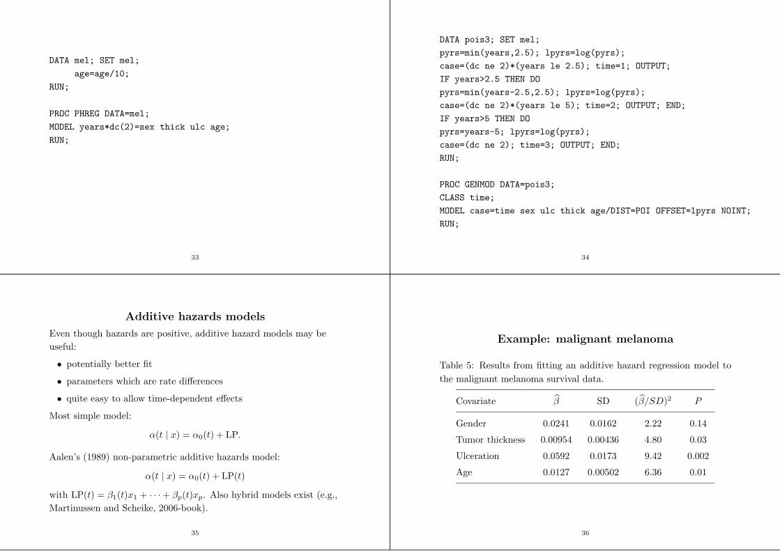
Additive hazards models

Even though hazards are positive, additive hazard models may be

useful:

• potentially better fit

• parameters which are rate differences

• quite easy to allow time-dependent effects

Most simple model:

α(t | x) = α0(t) + LP.

Aalen’s (1989) non-parametric additive hazards model:

α(t | x) = α0(t) + LP(t)

with LP(t) = β1(t)x1 + · · · + βp(t)xp. Also hybrid models exist (e.g.,

Martinussen and Scheike, 2006-book).

35

Example: malignant melanoma

Table 5: Results from fitting an additive hazard regression model to

the malignant melanoma survival data.

Covariate β SD (β/SD)2 P

Gender 0.0241 0.0162 2.22 0.14

Tumor thickness 0.00954 0.00436 4.80 0.03

Ulceration 0.0592 0.0173 9.42 0.002

Age 0.0127 0.00502 6.36 0.01

36

0 2 4 6 8

0.00

0.05

0.10

0.15

0.20

0.25

0.30

YearsC

umul

ativ

e re

gres

sion

func

tion,

Sex

0 2 4 6 8

0.0

0.1

0.2

0.3

0.4

0.5

Years

Cum

ulat

ive

regr

essi

on fu

nctio

n, U

lcer

atio

n

0 2 4 6 8

0.00

0.01

0.02

0.03

0.04

0.05

0.06

Years

Cum

ulat

ive

regr

essi

on fu

nctio

n, T

hick

ness

0 2 4 6 8

0.00

00.

005

0.01

00.

015

YearsC

umul

ativ

e re

gres

sion

func

tion,

Age

Figure 4: Melanoma data: cumulative regression functions from

Aalen’s additive model.

37

The increments of the cumulative regression functions are estimated

by solving a least squares equation at each failure point.

Tests for constant effects are available:

Table 6: Results from fitting Aalen’s additive hazard regression model

to the malignant melanoma survival data.

Covariate P : No Effect Time-Constant Effect

Gender 0.19 0.58

Tumor thickness 0.008 0.03

Ulceration 0.006 0.83

Age 0.05 0.33

38

R-, but no SAS-code

library(timereg)

summary(additivemodelConst <- aalen(Surv(years, dc != 2) ~

const(sex) + const(ulc) + const(I(thick-3)) + const(I(age-50)),

data = melanoma))

additivemodelNonConst <- aalen(Surv(melanoma$years,

melanoma$dc != 2) ~

sex + ulc + I(thick-3) + I(age-50), data = melanoma)

39

Accelerated failure time (AFT) models

These are not hazard models but ordinary linear models for the mean

log(life time):

E(log(T ) | x) = a + LP

or

log(T ) = a + LP + σε

where εi, i = 1, . . . , n i.i.d. with E(ε) = 0 Specifying the residual

distribution (i.e., for ε) this is a parametric regression model. For all

choices of that distribution (say, S0(·))

S(t | x) = S0(t exp(−LP)),

so time is accelerated by a factor exp(−LP) compared to x = 0.

40

Standard choices of residual distribution:

• Normal

• Logistic

• Extreme value: S0(w) = exp(−ew)

The latter choice is equivalent to a Weibull proportional hazards

model satisfying the relation:

βWeibull = −βAFT

σ,

and this is the only distribution belonging to both the proportional

hazards and the AFT class.

Semi-parametric inference for the AFT model is available via the

Buckley-James algorithm (however: convergence problems may

occur).

41

Example: malignant melanoma

Table 7: Results from fitting accelerated failure time regression models

to the malignant melanoma survival data.

Error Distribution Normal Extreme Value Weibull

Covariate β SD β SD β SD

Gender –0.522 0.262 –0.355 0.218 0.397 0.240

Tumor thickness –0.103 0.0438 –0.0864 0.0314 0.0967 0.0346

Ulceration –1.001 0.285 –0.866 0.252 0.969 0.269

Age –0.194 0.0786 –0.206 0.0669 0.231 0.0758

Intercept (a) 4.634 0.510 4.724 0.463

SD parameter (σ) 1.463 0.134 0.893 0.0939

42

R- and SAS-code

library(survival)

survreg(Surv(years, dc != 2) ~ sex + thick + ulc + I(age/10),

dist = "weibull", data = melanoma)

survreg(Surv(years, dc != 2) ~ sex + thick + ulc + I(age/10),

dist = "lognormal", data = melanoma)

PROC LIFEREG DATA=melanoma;

MODEL years*dc(2)=sex thick ulc age;

RUN;

PROC LIFEREG DATA=melanoma;

MODEL years*dc(2)=sex thick ulc age/DIST=lognormal;

RUN;

43

Survival data as a two-state model.

Alive

10

Dead-α(t)

Transition intensity

α(t) ≈ Pr(state 1 time t + dt | state 0 time t)/dt

State occupation probabilities

S(t) = Pr(state 0 time t), F (t) = 1 − S(t).

44

Competing risks as a multi-state model.

Alive

0

Dead, cause kk

QQ

QQ

QQs

Dead, cause 11

��

��

��3

α1(t)

αk(t)

p

p

p

45

Parameters.

Transition intensities: Cause-specific hazards, j = 1, . . . , k:

αj(t) ≈ Pr(state j time t + dt | state 0 time t)/dt,

State occupation probabilities:

S(t) = Pr(state 0 time t),

Fj(t) = Pr(state j time t), j = 1, . . . , k.

S(t) +k∑

j=1

Fj(t) = 1.

46

Mathematical formulation (1).

T , survival time, D cause of failure, joint distribution:

Pr(T ≤ t, D = j).

Cause-specific hazards:

αj(t) = lim∆→0

Pr(T ≤ t + ∆, D = j | T ≥ t)

∆.

Marginal distribution of T : survival function

S(t) = Pr(T > t) = exp(−∑

j

∫ t

0

αj(u)du).

Total hazard is α(t) =∑k

j=1 αj(t).

47

Mathematical formulation (2).

Latent failure times

T L1 , . . . , TL

k ,

observe min{T L1 , . . . , TL

k } and corresponding D.

Joint survival distribution:

Q(t1, . . . , tk) = Pr(T L1 > t1, . . . , T

Lk > tk).

Relations between the two formulations:

S(t) = Q(t, . . . , t),

αj(t) = −∂ log Q(t1, . . . , tk)

∂tj⌋t1=···=tk=t.

48

Parameter identification.

Which parameters may be identified from the right-censored

competing risks data (Ti, Di), i = 1, . . . , n, independent, where either

Ti = Ti and Di ∈ {1, . . . , k} or Ti > Ti and Di = 0?

Likelihood:∏

i S(Ti)∏

j(αj(Ti))I(Di=j).

From this we may identify the cause specific hazards αj(t) but not

the whole joint distribution Q(·) of the “latent failure times”

T L1 , . . . , TL

k .

For instance not the “marginal distribution” of T Lj :

Pr(Tj > tj) = Q(0, . . . , 0, tj , 0, . . . , 0) = Sj(tj)

with (“net”) hazard function hj(t) = −∂ log Sj(t)/∂t.

49

“Independent” competing risks.

Definition: T L1 , . . . , TL

k are independent, i.e. Q(t1, . . . , tk) =∏

j Sj(tj)

or (weaker): marginal (or “net”) and cause-specific (“crude”) hazards

are identical: αj(t) = hj(t).

Since Sj(t) and hj(t) cannot be identified from the data (without

further, unidentifiable conditions) these assumptions are unverifiable.

Likewise: the question of “what would happen if certain causes were

removed” is quite hypothetical in most biological settings (e.g.,

Kalbfleisch and Prentice, 2002; Andersen and Keiding, 2012).

(Sensitivity analysis?)

Possible exception: failure of technical systems due to components in

“unrelated parts” of the system.

50

“Counterexample”.

Kalbfleisch and Prentice (2002). Let k = 2 and:

Q(t1, t2) = exp(1 − α1t1 − α2t2 − exp(α12(α1t1 + α2t2))).

Cause-specific hazards: αj(t) = αj(1 + α12 exp(α12(α1 + α2)t)).

If α12 = 0 then risks 1 and 2 are “independent”. However, likelihood

would be the same if the model was

Q∗(t1, t2) = exp(1 − α1t1 − α2t2)

× exp(−α1e

α12(α1+α2)t1 + α2eα12(α1+α2)t2

α1 + α2)

risks are independent (also for α12 6= 0); cause-specific hazards are

the same (but marginal hazards are different).

51

Identifiable probabilities.

These are the state occupation probabilities in the competing risks

multi-state model. That is,

the overall survival function:

S(t) = exp(−∑

j

∫ t

0

αj(u)du),

and the cumulative incidences:

Fj(t) =

∫ t

0

S(u−)αj(u)du, j = 1, . . . , k.

-t t t t

0 u u + du t

time

52

Inference for cause-specific hazards.

Likelihood:n∏

i=1

S(Ti)k∏

j=1

(αj(Ti))I(Di=j)

=n∏

i=1

(exp(−

k∑

j=1

Aj(Ti))) k∏

j=1

(αj(Ti))I(Di=j)

=k∏

j=1

( n∏

i=1

exp(−Aj(Ti))(αj(Ti))I(Di=j)

).

Note:

• Product over causes, j,

• The jth factor is what we would get if only that cause was

studied and all other causes were right-censorings

53

Inference for cause-specific hazards.

• This has nothing to do with “independence” of causes - it is

solely a consequence of the definition of cause-specific hazards as

hazards of exclusive events.

• It means that all standard hazard-based models for survival data

apply when analyzing cause-specific hazards

– non-parametric: estimate Aj(t) =∫ t

0αj(u)du, j = 1, . . . , k by

Nelson-Aalen estimator, compare using, e.g. logrank tests

– parametric models

– Cox regression, Poisson regression

– ...

54

Malignant melanoma

Table 8: Results from fitting Cox regression models for the cause-

specific hazards in the malignant melanoma study.

All Causes Disease Other Causes

Covariate β SD β SD β SD

Gender 0.413 0.240 0.433 0.267 0.358 0.549

Tumor thickness 0.0994 0.0345 0.109 0.0377 0.0496 0.0879

Ulceration 0.952 0.268 1.164 0.310 0.109 0.591

Age 0.218 0.0775 0.121 0.0830 0.725 0.217

55

R- and SAS-code

library(survival)

## Death from all causes

(all <- coxph(Surv(years, dc != 2) ~ sex + thick + ulc +


## Death from malignant melanoma

(malmel <- coxph(Surv(years, dc == 1) ~ sex + thick + ulc +


## Death from other causes

(malmel <- coxph(Surv(years, dc == 3) ~ sex + thick + ulc +


56

/* Death from all causes */


MODEL years*dc(2)=sex thick ulc age; RUN;

/* Death from malignant melanoma */


MODEL years*dc(2,3)=sex thick ulc age; RUN;

/* Death from other causes */


MODEL years*dc(1,2)=sex thick ulc age; RUN;

57

Cumulative incidences.

Recall:

Fj(t) =

∫ t

0

S(u−)αj(u)du, j = 1, . . . , k

=

∫ t

0

exp(−k∑

h=1

Ah(u−))αj(u)du, j = 1, . . . , k.

Note that Fj(t), via S(u) = exp(−∑k

h=1 Ah(u−)), depends on the

cause-specific hazards for all causes.

That is, the simple one-to-one correspondance between the “rate”,

αj(t), and the “risk”, Fj(t), which we are used to from simple survival

analysis does no longer hold when competing risks are operating.

This is the key to understanding competing risks (e.g., Andersen et

al., IJE, 2012).

58

Inference for cumulative incidences.

Estimate for Fj(t): plug-in.

For simple non-parametric inference, plugging the Nelson-Aalen

estimator into Fj(t) gives the estimator

Fj(t) =

∫ t

0

S(u−)dAj(u),

where S is the Kaplan-Meier estimator for the overall survival

function, S.

This is a simple special case of the general Aalen-Johansen (1978)

estimator for non-homogeneous Markov processes.

A variance estimator is also available.

59

Sidetrack.

In the competing risks model, what is the interpretation of

Fj(t) = 1 − exp(−

∫ t

0

αj(u)du)?

It is: Pr(Dead from cause j before t) if all other αh(t) = 0, i.e. if the

competing risks did not exist!

It can, therefore, only be interpreted in a hypothetical population

where mortality from causes other than cause j have been eliminated

(and where the mortality from cause j is still given by the same αj(t)

- ”independent competing risks”).

This is an untestable assumption and the estimator F j(t) should not

be used.

60

It has, in fact, been used extensively in, e.g. clinical cancer studies:

“Relapse survival curve”.

The paradox is that Aj(t), the cumulative cause-specific hazard, is

not problematic (except for the fact that a cumulative hazard is hard

to interpret), but presenting this as a “Kaplan-Meier-type” estimator

is problematic since this does not have a probability interpretation.

The magnitude of this problem, obviously, depends on the magnitude

of the competing risk; but note that we always have: Fj(t) ≥ Fj(t).

61

R- (and SAS-)code

library(cmprsk)

attach(melanoma)

plot(cuminc(years,dc,,,cencode=2))

In SAS, various macros are available.

62

Figure 5: Malignant melanoma study: Cumulative incidence of dying

from the disease (solid curve) and from other causes (dashed curve).

0 5 10 15

0.0

0.2

0.4

0.6

0.8

1.0

Years

Pro

babi

lity

1 11 3

63

Regression models for competing risks

• Models for rates (cause-specific hazards):

– all well-known hazard regression models from survival analysis

• Models for risks (cumulative incidences):

– plug in models for rates: no simple covariate effects, but

prediction of cumulative incidence for given covariates is

possible. Standard errors available via the delta-method (Cox

model: Andersen, Hansen and Keiding (1992, SJS); additive

hazard model: Shen and Cheng (1999, Biometrics); flexible

“Cox-Aalen” model: Scheike and Zhang (2003, Biometrics)).

64

– Direct regression models

∗ Fine & Gray (1999, JASA), cloglog model: (Sub-distribution)

hazard for T ∗j = T · I(D = j) + ∞ · I(D 6= j) is

αj(t) = − ddt log(1 − Fj(t)), model:

log(αj(t | Z)) = log(αj0(t)) + βTZ where β is estimated by partial

likelihood with no or known censoring and by an IPCW score

equation with general censoring. Related to the Gray (1988, Ann.

Statist.) test for comparison of cumulative incidences.

∗ Fine (1999, JRSS B, 2001, Biostatistics), general links; Gerds et al.

(2012), log-link.

∗ pseudo-observations (Andersen, Klein et al., Biometrika, 2003;

Biometrics, 2005; SJS, 2007),

∗ Direct binomial regression using inverse probability of censoring

weights (Scheike & Zhang, 2007, SJS, Scheike, Zhang & Gerds

Biometrika, 2008)

65

R-code

library(cmprsk)

attach(melanoma)

cov<-matrix(nrow=205,ncol=2)

cov<-melanoma[,6:7] #just select ulceration and thickness

summary(crr(years,dc,cov,,,,failcode=1,cencode=2))

66

Table 9: Results from fitting Fine-Gray regression model for the risk

of dying from the disease in the malignant melanoma study.

Covariate β SD

Ulceration 1.173 0.303

Tumor thickness 0.0997 0.0358

Interpretation: exp(β) is a sub-distribution hazard ratio.

Sub-distribution hazard:

αj(t) ≈ Pr(X(t + dt) = j | X(t) 6= j)/dt,

i.e. conditioning is on either being alive or having failed from other

causes before t.

67

Time-dependent covariates

Hazard function with time-fixed covariates:

α(t | x) ≈ Pr(T ≤ t + dt | T > t, x)/dt.

This “definition” immediately allows covariates, x to be

time-dependent x(t) and conditioning may be on the entire past of

the covariate process:

α(t | x) ≈ Pr(T ≤ t + dt | T > t, (x(s), s ≤ t))/dt.

Cox’s likelihood:

L(β) =∏

i

( exp(LPi(Ti))P

j∈Riexp(LPj(Ti))

)Di.

Also Aalen’s additive model may be analysed with time-dependent

covariates which have to be updated when solving least squares

equations at each time of failure.

68

Time-dependent covariates

However, the relation

S(t | x) = exp(−

∫ t

0

α(s | x)ds)

may be lost when x depends on time.

Condition for the relation to hold: x(t) is exogenous (or external):

α(t | (x(s), s ≤ t)) = α(t | (x(s), s ≤ u)), for all u : t ≤ u,

e.g., Yashin and Arjas (J. Appl. Prob., 1988).

If x(t) is not exogenous then it is endogenous (internal).

69

Time-dependent covariates: examples

• deterministic, e.g. age at time t (given age at entry), exogenous

• time by covariate interactions, e.g. x · log(t), exogenous. Useful

for tests for proportional hazards (PBC-3 example below).

• air pollution recorded during follow-up, exogenous

• repeated (follow-up) measurements of covariates, e.g. bilirubin

and albumin recorded at follow-up visits to the hospital in the

PBC-3 study, endogenous

• complications or other events which may occur during follow-up,

e.g. local metastases (relapse) in melanoma patients, or Stanford

heart transplantations, endogenous

70

Endogenous time-dependent covariates

The hazard model no longer specifies the distribution of T .

Predictions may be performed by

1. a joint model for T and the process x(·)

2. landmarking

Joint model, e.g. malignant melanoma:

• Use the hazard model with the time-dependent covariate x(t) = 1

if relapse before t, x(t) = 0 otherwise, e.g.

α(t | (x(s), s ≤ t)) = α0(t) exp(LP + γx(t) + ρx(t)(t − Trel)).

• Supplement with a hazard model for x(t), e.g.

Pr(x(t + dt) = 1 | T > t, x(t−) = 0, x) ≈ θ0(t) exp(LPrel)dt.

71

The illness-death model

No relapse10

Relapse

Dead

-

2

SS

SSw

��

��/

θ(t)

α(t | x(t) = 0) α(t | x(t) = 1)

72

“Landmark” analysis.

Classical method from cancer research for evaluation of effect of

response to treatment on survival (Anderson, Cain, Gelber, 1983,

Cancer Research)

Discussed and extended by van Houwelingen (2007, Scand. J.

Statist.) Also Book by van Houwelingen and Putter (2011).

Idea: to assess the effect of time-dependent covariates on survival, set

up regression models at a series of “landmark” points s1, s2, ..., that

is, make a model for

Pr(T ≤ t + dt | T > t, (x(u), u ≤ sj)), t > sj ,

e.g. via a Cox model with time-fixed covariates.

van Houwelingen studied models where both baseline hazards and

regression coefficients vary smoothly with sj .

73

Test for proportional hazards

PBC-3 study, add covariate by time interactions to study

proportional hazards.

Table 10: PBC-3 study: tests for proportional hazards for treatment

and other covariates.

Covariate, x f(t) Effect of xf(t) Treatment Effect

bβ SD (bβ/SD)2 P bβ SD

Treatment log(t) 0.093 0.257 0.13 0.72

Treatment t 0.031 0.180 0.03 0.86

Albumin log(t) 0.034 0.027 1.54 0.22 –0.573 0.224

log(bilirubin) log(t) –0.092 0.130 0.51 0.48 –0.553 0.225

log(bilirubin) t –0.073 0.092 0.62 0.43 –0.548 0.225

Age log(t) 0.024 0.013 3.62 0.06 –0.570 0.225

74

R- and SAS-code

library(survival)

model1 <- coxph(Surv(followup, status != 0) ~ tment + alb +

log(bili) + log(alkph) + log(asptr) + age, data = pbc3)

pbc3$event <- ifelse(pbc3$status != 0, 1, 0)

eventtimes <- survfit(model1)$time

pbc3.split <- survSplit(pbc3, cut = eventtimes, start = "start",

end = "followup", event = "event", id = "ptno")

pbc3.split$end <- pbc3.split$followup

75

coxph(Surv(start, end, event) ~ tment + alb + log(bili) +

log(alkph) + log(asptr) + age +

ifelse(tment == "1", log(end), 0), data = pbc3.split)


MODEL followup*status(0)=tment alb logbili logalkph

logast age tmenttime;

tmenttime=tment*log(followup);

RUN;

76

The illness-death model

No illness

10Ill

Dead

-

2

SS

SSw

��

��/

α01(t)

α02(t) α12(t)

The illness-death model is a useful multi-state model in its own right

(e.g., Andersen and Keiding, 2002, SMMR). It has had a recent

revival (focussing, unfortunately on “wrong” aspects!) under the

name semi-competing risks (e.g., Fine et al., Biometrika, 2001).

77

References/Bibliography.OO Aalen (1978). Ann. Statist. 6, 534.

OO Aalen (1989). Stat. in Med. 8, 907.

OO Aalen, Ø Borgan, HK Gjessing (2008). Survival and Event History Analysis.

Springer.

OO Aalen, S Johansen (1978). Scand. J. Statist. 5, 141.

PK Andersen, Ø Borgan, RD Gill, N Keiding (1993). Statistical Models Based on

Counting Processes. Springer

PK Andersen, LS Hansen, N Keiding (1991). Scand. J. Statist. 18, 153.

PK Andersen N Keiding (2002). Statist. Meth. Med. Res. 11, 91.

PK Andersen N Keiding (2012). Statist. in Med. 31, (in press).

PK Andersen, JP Klein, S Rosthøj (2003). Biometrika 90, 15.

PK Andersen, JP Klein (2005). Biometrics 61, 223.

PK Andersen, JP Klein (2007). Scand. J. Statist. 34, 3.

PK Andersen, RB Geskus, T de Witte, H Putter (2012). Int. J. Epi. 41 (in press).

PK Andersen, LT Skovgaard (2010). Regression with Linear Predictors. Springer.

JR Anderson, KC Gain, RD Gelber (1983). J. Clin. Oncol. 1, 710.

78

N E Breslow (1974). Biometrics 30, 89.

D Clayton, M Hills (1993). Statistical Models in Epidemiology. Oxford.

D Collett (2003). Modeling Survival Data in Medical Research. Chapman and

Hall/CRC.

DR Cox (1972). J. Roy. Statist. Soc. B 34, 187.

DR Cox (1975). Biometrika 62, 269.

DR Cox, D Oakes (1984). Analysis of Survival Data. Chapman and Hall.

JP Fine (1999). J. Roy. Statist. Soc. B 61, 817.

JP Fine (2001). Biostatistics 2, 85.

JP Fine, H Jiang, R Chappell (2001). Biometrika 88, 907.

JP Fine, RJ Gray (1999). J. Amer. Statist. Assoc. 94, 496.

TA Gerds, TH Scheike, PK Andersen (2012). Stat. in Med. (in press).

18, 695.

RJ Gray (1988). Ann. Statist. 16, 1141.

JD Kalbfleisch, RL Prentice (2002): The Statistical Analysis of Failure Time Data,

2nd ed.. Wiley.

EL Kaplan, P Meier (1958). J. Amer. Statist. Assoc. 53, 457.

79

M Lombard et al. (1993). Gastroenterology 104, 519.

T Martinussen, TH Scheike (2006). Dynamic Regression Models for Survival Data.

Springer.

TH Scheike, M-J Zhang (2003). Biometrics 59, 1036.

TH Scheike, M-J Zhang (2007). Scand. J. Statist. 34, 17.

TH Scheike, M-J Zhang, TA Gerds (2008). Biometrika 95, 205.

Y Shen, SC Cheng (1999). Biometrics 55, 1093.

HC van Houwelingen (2007). Scand. J. Statist. 34, 70.

HC van Houwelingen, H Putter (2011). Dynamic Prediction in Clinical Survival

Analysis. Chapman and Hall/CRC..

A Yashin, E Arjas (1988). J. Appl. Prob. 25, 630.

80

per kragh andersen, university of copenhagen, denmark analysis

Documents