people are variables too: multilevel structural equations modeling

People Are Variables Too: Multilevel Structural Equations Modeling

Paras D. MehtaUniversity of Houston

Michael C. NealeVirginia Commonwealth University

The article uses confirmatory factor analysis (CFA) as a template to explain didacticallymultilevel structural equation models (ML-SEM) and to demonstrate the equivalence ofgeneral mixed-effects models and ML-SEM. An intuitively appealing graphical representa-tion of complex ML-SEMs is introduced that succinctly describes the underlying model andits assumptions. The use of definition variables (i.e., observed variables used to fix modelparameters to individual specific data values) is extended to the case of ML-SEMs forclustered data with random slopes. Empirical examples of multilevel CFA and ML-SEM withrandom slopes are provided along with scripts for fitting such models in SAS Proc Mixed,Mplus, and Mx. Methodological issues regarding estimation of complex ML-SEMs and theevaluation of model fit are discussed. Further potential applications of ML-SEMs areexplored.

Keywords: multilevel modeling, structural equations modeling, multilevel-structural equa-tions modeling, multilevel-confirmatory factor analysis, mixed effects models

Multilevel modeling (MLM) and structural equationsmodeling (SEM) have evolved from different conceptualand methodological roots. The former deals with the anal-ysis of clustered data (e.g., students nested within class-rooms) and attempts to partition observed variance intowithin- and between-clusters components.1 The latter dealswith modeling means and covariances among multivariatedata. The two classes of models focus on different questions

and have different strengths and weaknesses. Because bothclustered and multivariate data are common and of muchsubstantive interest, it is not surprising that practitioners ofeach method are interested in borrowing strengths of theother (Goldstein & McDonald, 1987; Krull & MacKinnon,2001; McDonald, 1993; Muthen, 1989; Muthen & Satorra,1995; Raudenbush, 1995; Raudenbush & Sampson, 1999).Although considerable advances have been made in thisrespect, structural modeling of multilevel data is a relativelynew area of methodological research (Bauer, 2003; Bentler& Liang, 2003; Curran, 2003; du Toit & du Toit, 2003;Kaplan & Elliot, 1997; Muthen, 1991, 1994, 1997; Rovine& Molennar, 2000).

This article develops the notion of multilevel modeling aswell as multilevel structural equations modeling (ML-SEM)from within the SEM framework by borrowing commonand well-understood metaphors from measurement. In thebroadest sense, ML-SEM combines the best of both worlds.It allows full-blown SEM models to be developed at eachlevel of nesting for clustered data. For example, multipleindividual-level indicators can be used to define a latent

1 The term nesting and clustering are commonly used in themultilevel modeling literature to indicate data-nested structuressuch as students clustered or nested within classrooms. This notionof nesting is distinct from the notion of nested designs in ananalysis of variance context in that in MLM, the sampling units atboth levels are assumed to be sampled randomly. Hence, class-rooms are assumed to be sampled randomly from a universe of allpossible classrooms, and students are also assumed to be sampledrandomly within each classroom.

Paras D. Mehta, Texas Institute for Measurement Evaluationand Statistics, University of Houston; Michael C. Neale, VirginiaInstitute of Psychiatric and Behavioral Genetics, Virginia Com-monwealth University.

This work was supported by National Institute of Child Healthand Human Development Grant HD30995 (Early Interventions forChildren with Reading Problems), the National Institute of ChildHealth and Human Development, U.S. Department of Education’sInstitute of Education Sciences Grant HD39521 (Oracy/LiteracyDevelopment of Spanish-Speaking Children). Michael C. Nealewas supported by National Institute of Health Grants MH-65322(Psychopathology: Models, Measurement and Classification) andDA-18673 (Psychometric and Genetic Assessments of SubstanceUse).

We would especially like to thank Lee Branum-Martin, PatrickW. Taylor, and Chris D. Barr for their helpful comments on earlierversions of this article.

Additional materials are on the Web at http://dx.doi.org/10.1037/1082-989X.10.3.259.supp

Correspondence concerning this article should be addressed toParas D. Mehta, Department of Psychology, University of Hous-ton, 126 Heyne Building, Houston, TX 77204-5022. E-mail:[email protected]

Psychological Methods2005, Vol. 10, No. 3, 259–284

Copyright 2005 by the American Psychological Association1082-989X/05/$12.00 DOI: 10.1037/1082-989X.10.3.259

259

construct at the individual level as well as at the clusterlevel, and, mediational hypotheses can be evaluated at bothlevels. Finally, the article demonstrates how random slopesmay be incorporated into ML-SEM for clustered data.

Repeated measures data are inherently multilevel, withrepeated measurements on an outcome measure nestedwithin each individual. It is therefore not surprising thatmodels of individual growth were initially conceptualizedwithin the MLM framework (Raudenbush & Bryk, 2002). Itwas in the context of latent growth curves (LGC) thatWillett and Sayer (1994) demonstrated how models of in-dividual change could be fitted using conventional meansand covariance structure analysis with time-structured data(see also Chou, Bentler, & Pentz. 1998; MacCallum, Kim,Malarkey, & Keicolt-Glaser, 1997; Meredith & Tisak,1990). A critical assumption of the means- and covariance-based LGCs is that the time interval between measurementoccasions must be equal across individuals. The availabilityof raw data or full-information maximum likelihood esti-mation (FIML) in popular SEM software partially alleviatedthe limitation of equal time intervals (Arbuckle, 1996;Neale, 2000b). The missing-data handling capability ofFIML was exploited in order to allow unequal intervalsbetween measurement occasions in growth curve analysis(Duncan, Duncan, & Hops, 1996; McArdle & Anderson,1990). In this missing data approach, an outcome measuredat each time point is treated as a separate variable. Hence,each individual will have data at some but not at all timepoints, allowing unequal intervals between measurementoccasions. This approach is impractical when there is con-siderable heterogeneity in time of the first occasion or in theintervals between occasions of measurement. Mehta andWest (2000) demonstrated the use of the individual-likeli-hood based SEM estimation along with the special data-handling facility for estimating the parameters of LGCmodels with continuous values of time. The current articleextends the idea of estimating random slopes for continuouspredictors to clustered data (e.g., students nested withinclassrooms) and multivariate outcomes.

The missing data approach has also been extended to thecontext of multilevel modeling of clustered data. In a set ofrelated articles, Bauer (2003) and Curran (2003) demon-strated the applicability of SEM models to clustered data inthe context of both balanced and unbalanced designs. Bauerapplied two alternate approaches to missing data in longi-tudinal setting (Mehta & West, 2000) to the clustered datacase. Both Bauer and Curran provided practical examples ofhow such models can be fit in conventional software. Con-sistent with Rovine and Molenaar (2000), Bauer demon-strated the equivalence between SEM and univariate mixed-effects model (MEM) matrices. Curran graphicallypresented possible extensions of the univariate random-intercepts model to the case of multiple latent variables atthe individual and the cluster levels.

The primary purpose of this article is to introduce the

ML-SEMs in a didactic fashion using concepts that are wellunderstood in the context of conventional SEM. This isaccomplished by developing core ML-SEMs as variants ofthe restricted confirmatory factor analysis (CFA) in whichfactor loadings are not estimated but are fixed by design. Weshow how reframing such MLMs as restricted CFA modelsreadily allows parameter estimation by individual likeli-hood. Finally, we show how person-specific data may beused for modeling means, as well as covariances, at anindividual level. As is explained later, the ability to modelperson-specific covariances is central to modeling randomslopes in conventional MLMs.

Several alternative representations exist for specifyingand estimating MLMs of varying degrees of complexitywithin specific software such as HLM (Bryk, Raudenbush,Seltzer, & Congdon, 1988), MLwiN (Rasbash et al., 2000),and SAS Proc Mixed (SAS Institute, 1996). The mapping ofone specification onto another, especially for multivariateoutcomes, is not obvious to the uninitiated. ML-SEMs rep-resent a considerable advance over conventional MLMs,considering the fact that the majority of applications ofmultilevel modeling are restricted to univariate outcomes.As such, representation of MLMs within the multivariateSEM-oriented scripting language such as Mplus (Muthen &Muthen, 2004) is even less obvious.

The current article aims to clarify the interrelationshipsamong the different representational schemes by graphicallyusing an extended RAM (recticular action model) represen-tation (McArdle & Boker, 1990) of an ML-SEM.2 Scalarrepresentations of univariate and multivariate MLM mapdirectly on to this multilevel graphical representation of arestricted CFA model. Additionally, the SEM matrices forthe CFA model bear a one-to-one correspondence with thematrices of the general MEM. Finally, the notion of arandom slope for a continuous predictor fits within thisextended graphical representation simply as a fixed factor

2 There are several alternative but highly similar graphical rep-resentations of SEM. The RAM notation is similar to other nota-tion in that it uses rectangles and circles to represent observed andlatent variables, respectively. In addition, like other representa-tions, it uses curved double-ended arrows and directed arrows torepresent covariances and variances, respectively. Because vari-ances may be thought of as the covariance of a variable with itself,the RAM notation uses curved double-ended arrows to representunconditional and conditional or residual variances. Finally, theRAM notation uses a directed arrow from a triangle to an observedor latent variable to represent unconditional or conditional mean.The triangle represents a fixed constant of 1.0 for each individual;hence, the directed path can be interpreted as the mean (or theintercept). An important consequence of RAM notation is that allof the model parameters are explicitly represented in a path dia-gram. As a result, the graphical representation can be computa-tionally transformed into its underlying mathematical representa-tion (see Neale, Boker, Xie, & Maes, 2004).

260 MEHTA AND NEALE

loading. It is hoped that the universal graphical representa-tion will help researchers familiar with either class of mod-els to conceptualize and fit models within the more generalML-SEM context.

ML-SEM: The Building Blocks

Three critical ideas necessary for understanding ML-SEMs are (a) the concept of a restricted CFA model, (b) thenotion of individual likelihood, and (c) the related idea ofmodeling individual-specific data vectors. These buildingblocks are used to construct ML-SEMs for clustered data ina bottom-up fashion.

CFA

The pattern of means and covariances of MLMs is iden-tical in form to that of CFA. CFA can therefore serve as atemplate for formulating MLMs. The relation between thetwo classes of models has been recognized in univariate andmultivariate SEM formulations of latent growth (MacCal-lum et al., 1997; Willett & Sayer, 1994) as well as explicitMLM models (Rovine & Molenaar, 2000). At a practicallevel, the template can be easily adapted to specify and fitmore complex MLMs. For example, multilevel latent vari-able models have been conceptualized as hierarchical factormodels (Bauer, 2003; Curran, 2003).

Apart from the similarity in the data structure (i.e., nestingand unbalanced data) and the scalar representations of growthcurves and multilevel regression models, there are importantdifferences between the two classes of models. For example,unlike variables ordered in time, individuals within a cluster donot have a specific order. Such similarities and differencesamong different MLMs lead to a specific set of expectationsregarding the structure imposed on the data as well as distri-butional assumptions (e.g., conditional independence and ho-moscedasticity) for the latent variables and residuals at eachlevel. To the extent that the chosen factor model templateadequately captures the underlying assumptions of MLMs, theuse of CFA as a template is appropriate. The current articlesummarizes the critical implicit assumptions in SEM modelsfor clustered data. For example, the hierarchical factor modelrepresentation of latent variable models of multivariate clus-tered data implies a set of falsifiable restrictions on the general-specific factor model (Gustafsson, 2002; Gustafsson & Balke,1993).

CFA aims to explain the covariance among p observedvariables (Yp) in terms of q latent variables (�q). All un-specified sources of variability including error and specificfactors are labeled as residuals, epi:

Ypi � �p � �pq�qi � epi, (1)

where for an individual i, Ypi is the score for the pthobserved variable, and �qi is the score for the qth latentvariable, and epi is the residual or the error term for the pth

observed variable. The factor loadings (�pq) reflect themagnitude of change in the observed variable (Yp) for unitchange in the latent variable (�q), and �p is the measurementintercept. The model implied mean vector is

� � � � ��, (2)

where � is a q � 1 vector of latent variable means,3 and thecovariance � (p � p) is

� � �� , (3)

where � (q � q) is the latent variable covariance matrix,and � (p � p) is a diagonal matrix containing residualvariances.

Individual Likelihood Based SEM

The second building block necessary for understandingML-SEMs is the notion of fitting SEM models to individualdata vectors. The conventional means- and covariance-based SEM is limited to complete data. Cases with missingdata are typically eliminated in a listwise fashion. FIMLestimation was introduced in SEM as a means of handlingmissing data (Arbuckle, 1996; Neale, 2000b). The bulk ofdiscussion regarding the limitations of the SEM approach toclustered data has focused on its inability to deal withunbalanced data (Bauer, 2003; Curran, 2003; Mehta &West, 2000; Willett & Sayer, 1994). This is not a limitationof the model per se, but instead reveals two related issuescontributing to the inflexibility of the SEM framework: (a)the use of the sample means- and covariance-based estima-tion approach and (b) data handling and structuring issuesthat make such models difficult to formulate in a script andalso make such models computationally inefficient to esti-mate. The availability of estimation methods based on in-dividual likelihood makes it possible to specify and estimatefairly complex models that naturally accommodate unbal-anced data structures. In this approach, likelihood is com-puted using individual data vectors. Assuming multivariatenormality among the observed outcomes, the likelihood of aspecific response vector is

Prob�yi� � �2��p/ 2|�|�1/ 2exp� � 0.5�yi � ��1�yi � ��,

where � is a vector (p � 1) of means of the variables, and� is the covariance matrix (p � p); �� and ��1are thedeterminant and inverse of the covariance matrix, respec-tively. For any given � and �, twice the negative loglikelihood of an individual data vector (yi) is

3 Latent variable mean is typically represented by the Greeksymbol �. In this article, we use to represent latent variablemeans in order to be consistent with the fixed-effects vector in amultilevel model.

261MULTILEVEL STRUCTURAL EQUATIONS MODELING

�2LogLi � Ki � log|�i| � �yi � �i��i�1�yi � �i�, (4)

where Ki� pi log(2�). The ML fit function for an indepen-dent sample of observations is obtained by summing theindividual �2LL over all the number of individuals:�2LogLS � �i�1

N (�2LogLi). The person-specific likeli-hood allows missing data without listwise deletion. Underthe assumption of missing at random, conditional on theobserved data, the expected individual-specific means andcovariances for the variables that are missing for an indi-vidual are equal to the corresponding means and covari-ances for an individual with complete data. During estima-tion, the model implied mean and covariance matrices arecomputed for each unique response pattern. The variablesthat are missing are simply eliminated from the individual’smean and covariance matrix. In other words, the dimensionof the covariance matrix varies across individuals, depend-ing on the number of observations actually present for thatindividual.

Modeling Individual-Specific Covariances: DefinitionVariables

There is an equally important but little recognized by-prod-uct of estimation based on individual likelihood. FIML offersthe possibility of fitting new types of models in which themodel-implied means and covariances are different for eachindividual. The notion of modeling means in terms of thepredictors is central to ordinary multiple regression as well asSEM; however, the notion of modeling covariance as a func-tion of predictors is fairly novel. In SEM, multiple-groupmodeling is used to account for differences in covariancesacross discrete grouping variables. It is also plausible that thecovariances among dependent variables may vary as a functionof continuous-valued predictors. For example, the covariance(and variances) between latent variables stress and symptomsmay be continuous functions of neuroticism:

�stress,symptoms�i � f�neuroticismi�.

In this case, there is no single sample covariance matrix.Instead, there are as many covariance matrices as there

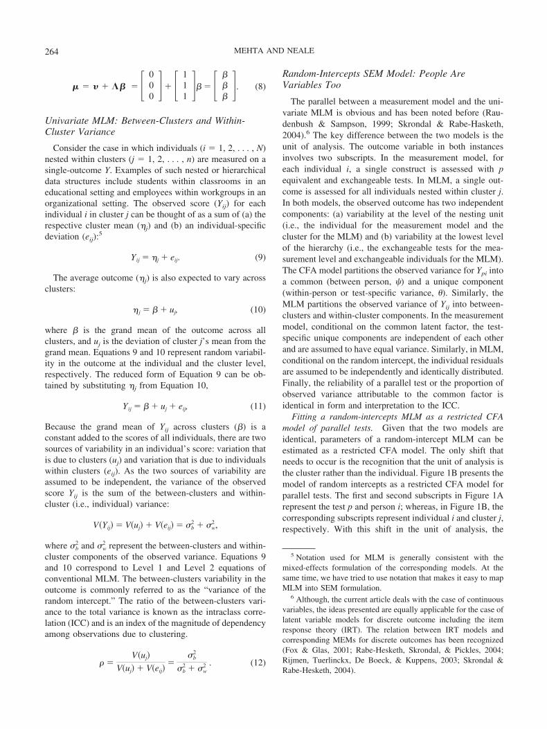
Figure 1. A: Restricted confirmatory factor analysis (CFA)model of parallel tests. Observed scores of all p variables (Ypi) forindividual i load on a common individual-level latent variable (�i)with all factor loadings equal to 1.0. Dashed line indicates vari-ables not included in the figure. Residual variances for all pobserved variables are assumed to be equal (�). Latent factor meanis not represented in the figure. B: Univariate random-interceptsmodel represented as a restricted CFA model. Observed scores ofall individuals (Yij) in cluster j are allowed to load onto a commoncluster-level latent variable (�j) with all factor loadings equal to1.0. The cluster-level latent variable represents the random effectfor the jth cluster. Dashed line indicates scores of individuals notincluded in the figure. Within-cluster residual variance is assumedto be equal for all individuals. Latent factor mean (i.e., the grand

mean of the dependent variable) is not represented in the figure. C:Succinct representation of univariate random-intercepts model.The figure represents the model for a single individual (i) nested incluster (j). The within- and between-clusters variables are identi-fied by appropriate subscripts. The observed variable includes bothperson (i) and group (j) subscripts, indicating that the observedscores of all individuals within a given cluster load onto thecommon cluster-level latent variable (�j) with all factor loadingsequal to 1.0. It is assumed that the cluster-level latent variable (�j),and the individual-level residuals (�ij), are independently andidentically distributed with variances b

2 and w2 , respectively. This

critical assumption allows us to represent the model succinctly.

262 MEHTA AND NEALE

are distinct values of neuroticism present in the data.Hence, it might not just be impractical but impossible tofit a separate model for each discrete value of the pre-dictor. The individual likelihood allows person-specificmeans and covariances, so it is possible to compute thelikelihood separately for each individual, based on theirexpected means and covariances, conditional on the ob-served values of individual predictors.

Exogenous predictors used in this fashion are called “defi-nition variables.” Variables flagged as definition variables canbe used to fix the values of any model parameter, includingfactor loadings and variances. Such a facility is essential forfitting models with heteroscedastic errors and interaction be-tween latent and observed predictors (Muthen & Asparouhov,2002, 2003; Neal, 1998, 2000a, 2000b). Other examples of theuse of definition variables can be found in Eaves, Neale, andMaes (1996), Neale (2000a, 2003), and Silberg, Rutter, Neale,and Eaves (2001). Random slopes in MLM also implies thatcovariances are a function of some predictor. Hence, FIML iscentral to fitting ML-SEMs with random slopes. In the nextsection, we consider MLMs for a single outcome and illustratehow the random intercepts MLM has the same form as themodel of parallel tests in classical test theory (CTT). Hence,the random-intercepts MLM may be fitted as a restricted CFAmodel.

Univariate Multilevel Models Are ReallyMultivariate Unilevel Models

The notions of between-clusters and within-clustervariability in MLM parallel those of common and uniquesources of variability, respectively, in measurement mod-els (Skrondal & Rabe-Hesketh, 2004). In fact, the modelof parallel tests is mathematically identical to the randomintercepts model in MLM. Practically, this involvesswitching subscripts of a univariate MLM (people andclusters) with those of a CFA model (variables and peo-ple); that is, individual scores are conceptualized as sep-arate variables, and the unit of analysis for the SEMmodel is now the cluster.

Model of Parallel Tests: Common and UniqueSources of Variance

In CTT, the observed score Ypi for an individual i on a testp is thought of as being composed of two components: truescore and random error.

Ypi � Ti � epi, (5)

Note that Equation 5 is identical to Equation 1 for thegeneral CFA model in which the intercepts and factorloadings are fixed to 0.0 and 1.0, respectively, for all p tests:

Ypi � 0.0 � 1.0�i � epi,

where the latent variable (�i) represents the unobserved truescore. Figure 1A presents the CFA model of parallel tests.All p tests share a common origin (i.e., equal intercepts;�p � 0.0) and have the same unit of measurement (i.e.,equal loadings; �p � 1.0). The true score is assumed to bedistributed independently and identically, � N (�, �),and the residual variance for all p tests is assumed to beequal (�pp � �).4 In other words, all p tests are assumed tobe exchangeable; that is, if we select a random subset oftests from the universe of all parallel tests, we could fit therestricted CFA model in order to estimate the varianceattributable to the true score.

Because the factor loadings for all p observed variablesare equal to 1.0, the variance attributable to the true-scoreequals the variance of the latent factor ( ), often referred toas the “common variance.” The unique component (�pi) fora given test is independent of the residuals for the remainingtests and the true score (�i), and its variance is commonlyreferred to as the “unique variance” (�). The variance ofeach test is the sum of common variance ( ) and the uniquevariance (�).

V�Yp� � �p2V��p� � V�ep� � � �.

The reliability of a test is the ratio of the true-score varianceto the total variance:

rel�Yp� �True-score variance

Total variance�

�.

The covariance between any two tests is

CV�Yp,Yp�� pV��p� � 1* *1 � .

In other words, the covariance between any two paralleltests equals the true-score variance. For three parallel tests,the implied covariance is

� � �� 111�� 1 1 1 �

� � ��

��

� � � �

�. (7)

The structure of the covariance matrix remains the sameregardless of the number of tests: with equal off-diagonalelements containing the true-score variance and the totalvariance along the diagonals. Finally, all p means are equalto the latent factor mean:

4 CFA allows for the possibility of specific factors in residuals,whereas the strict CTT assumes that errors are random. For thecurrent purpose, the distinction is not critical, as we use CTTmerely as a metaphor rather than as a model in a strict sense.


� � � �� 000� � � 1

11� � �

�. (8)

Univariate MLM: Between-Clusters and Within-Cluster Variance

Consider the case in which individuals (i � 1, 2, . . . , N)nested within clusters (j � 1, 2, . . . , n) are measured on asingle-outcome Y. Examples of such nested or hierarchicaldata structures include students within classrooms in aneducational setting and employees within workgroups in anorganizational setting. The observed score (Yij) for eachindividual i in cluster j can be thought of as a sum of (a) therespective cluster mean (�j) and (b) an individual-specificdeviation (eij):

5

Yij � �j � eij. (9)

The average outcome (�j) is also expected to vary acrossclusters:

�j � � uj, (10)

where is the grand mean of the outcome across allclusters, and uj is the deviation of cluster j’s mean from thegrand mean. Equations 9 and 10 represent random variabil-ity in the outcome at the individual and the cluster level,respectively. The reduced form of Equation 9 can be ob-tained by substituting �j from Equation 10,

Yij � � uj � eij, (11)

Because the grand mean of Yij across clusters () is aconstant added to the scores of all individuals, there are twosources of variability in an individual’s score: variation thatis due to clusters (uj) and variation that is due to individualswithin clusters (eij). As the two sources of variability areassumed to be independent, the variance of the observedscore Yij is the sum of the between-clusters and within-cluster (i.e., individual) variance:

V�Yij� � V�uj� � V�eij� � b2 � w

2 ,

where b2 and w

2 represent the between-clusters and within-cluster components of the observed variance. Equations 9and 10 correspond to Level 1 and Level 2 equations ofconventional MLM. The between-clusters variability in theoutcome is commonly referred to as the “variance of therandom intercept.” The ratio of the between-clusters vari-ance to the total variance is known as the intraclass corre-lation (ICC) and is an index of the magnitude of dependencyamong observations due to clustering.

� �V�uj�

V�uj� � V�eij��

b2

b2 � w

2 . (12)

Random-Intercepts SEM Model: People AreVariables Too

The parallel between a measurement model and the uni-variate MLM is obvious and has been noted before (Rau-denbush & Sampson, 1999; Skrondal & Rabe-Hasketh,2004).6 The key difference between the two models is theunit of analysis. The outcome variable in both instancesinvolves two subscripts. In the measurement model, foreach individual i, a single construct is assessed with pequivalent and exchangeable tests. In MLM, a single out-come is assessed for all individuals nested within cluster j.In both models, the observed outcome has two independentcomponents: (a) variability at the level of the nesting unit(i.e., the individual for the measurement model and thecluster for the MLM) and (b) variability at the lowest levelof the hierarchy (i.e., the exchangeable tests for the mea-surement level and exchangeable individuals for the MLM).The CFA model partitions the observed variance for Ypi intoa common (between person, ) and a unique component(within-person or test-specific variance, �). Similarly, theMLM partitions the observed variance of Yij into between-clusters and within-cluster components. In the measurementmodel, conditional on the common latent factor, the test-specific unique components are independent of each otherand are assumed to have equal variance. Similarly, in MLM,conditional on the random intercept, the individual residualsare assumed to be independently and identically distributed.Finally, the reliability of a parallel test or the proportion ofobserved variance attributable to the common factor isidentical in form and interpretation to the ICC.

Fitting a random-intercepts MLM as a restricted CFAmodel of parallel tests. Given that the two models areidentical, parameters of a random-intercept MLM can beestimated as a restricted CFA model. The only shift thatneeds to occur is the recognition that the unit of analysis isthe cluster rather than the individual. Figure 1B presents themodel of random intercepts as a restricted CFA model forparallel tests. The first and second subscripts in Figure 1Arepresent the test p and person i; whereas, in Figure 1B, thecorresponding subscripts represent individual i and cluster j,respectively. With this shift in the unit of analysis, the

5 Notation used for MLM is generally consistent with themixed-effects formulation of the corresponding models. At thesame time, we have tried to use notation that makes it easy to mapMLM into SEM formulation.

6 Although, the current article deals with the case of continuousvariables, the ideas presented are equally applicable for the case oflatent variable models for discrete outcome including the itemresponse theory (IRT). The relation between IRT models andcorresponding MEMs for discrete outcomes has been recognized(Fox & Glas, 2001; Rabe-Hesketh, Skrondal, & Pickles, 2004;Rijmen, Tuerlinckx, De Boeck, & Kuppens, 2003; Skrondal &Rabe-Hesketh, 2004).

264 MEHTA AND NEALE

model-implied means and covariances for the restrictedCFA model are directly applicable to the model of randomintercepts.7 However, unlike the model of parallel tests, thenumber of participants is likely to vary across clusters.Hence, FIML estimation is essential for fitting a MLM as aCFA model. Representation of MLM for clustered data inFigure 1B follows directly from the representation ofgrowth curves for repeated-measures data (Willett & Sayer,1994). Such a graphical representation has been used forconceptualizing univariate and multivariate random-inter-cepts as well as random-slopes models for clustered data(Bauer, 2003; Curran, 2003). The differences between thetwo classes of model allow for the possibility of simplifyingthe representation. We now present a set of principles thatallow a translation of algebraic and distributional implica-tions of an MLM to a succinct but complete graphicalrepresentation.

Graphical representation of a univariate random-inter-cepts model. In conventional SEM, individuals are assumedto be sampled randomly and are thus assumed to be exchange-able. Hence, the graphical representation depicts the model fora single individual only. In Figure 1B, the latent variablerepresents the cluster level outcome �j, and each observedoutcome represents individual scores (Yij) for each individual iwithin cluster j. For this model, sampling units at both levels(i.e., clusters and individuals) are exchangeable. As a result, itis necessary to represent a single cluster and a single individualwithin that cluster. Figure 1C presents such a succinct graph-ical representation of a random-intercepts model for an indi-vidual i within cluster j. All three hypothesized parameters ofthe random-intercepts model are represented in Figure 1C, andthe diagram accurately and completely captures the underlyingmathematical model.8,9

So far we have shown that the equations for a mea-surement model and a random-intercepts model are iden-tical in form and interpretation. The presentation wasprimarily conceptual and used the hierarchical linearmodeling (HLM; Bryk & Raudenbush, 1987) specifica-tion. The next section presents an MEM formulation of amultivariate MLM. MEM allows us to draw direct par-allel among the matrices used in MLM and ML-SEM aswell as the corresponding likelihood equations. Althoughthe equivalence of MEM and SEM is rather trivial in thecase of the univariate random-intercepts model, demon-stration of a formal equivalence between MEM and CFAmodels in the general case allows us to represent complexMEMs as special cases of restricted CFA models.

The next section extends the equivalence of MEM andCFA models to the multivariate case. In this context, wegeneralize the extended RAM notation to incorporate mul-tivariate covariance structure at the within- and between-clusters level. The resulting within- and between-clusterscovariances form the basis of fitting SEM models at eachlevel. We demonstrate how latent variable measurementmodels may be fitted at both levels. In addition, we describe

the set of assumptions necessary for defining random inter-cepts of the individual-level latent variables.

Multivariate Multilevel Models Are AlsoMultivariate Unilevel Models

The key insight presented so far was that SEM could beused to analyze univariate outcomes for clustered data:(a) by treating clusters as the unit of analysis and (b) bytreating the outcome for each individual as a separateindicator of a cluster-level latent variable (i.e., randomeffect). For a single outcome, the focus was on partition-ing the observed variance into between-clusters and with-in-cluster variance (i.e., b

2 and w2 ). With multivariate

outcomes and clustered data, we must consider the be-tween-clusters and within-cluster covariance matrices(i.e., �b and �w; see also Goldstein, 2003; Hox, 2002;Raudenbush, 1995; Raudenbush, Rowan, & Kang, 1991;Thum, 1997; Yang, Goldstein, Browne, & Woodehouse,2001). A multivariate extension of the random interceptsmodel can also be conceptualized as a restricted CFAmodel. The SEM representation of a bivariate MLM forPij and Qij is presented next.

Bivariate MLM: Between-Clusters and Within-Cluster Covariance

The univariate random-intercepts model may be extendedfor two outcome variables as

YijP � P � uj

P � eijP and Yij

Q � Q � ujQ � eij

Q (13A & 13B)

where P and Q are the grand means of P and Q, respectively,uj

P and ujQ are deviations of cluster j’s means of P and Q from

their respective grand means, and eijP and eij

Q are individual i’sdeviation scores on the two outcomes from their respectivecluster means. The between-clusters random effects (uj

P and

7 Additional materials, including annotated scripts in SAS ProcMixed, Mplus, and Mx, as well as various datasets, are on the Webat http://dx.doi.org/10.1037/1082-989X.10.3.259.supp

8 Note that when the assumption of independent clusters orexchangeable individuals is not justified, the graphical representa-tion must be modified accordingly. Such instances may arise, forexample, with data from multiple siblings in which birth order isimportant, or for dyadic couples data, or when the same teacherteaches multiple classrooms in school data.

9 Similar notion of exchangeability has been used for graphi-cally representing general multilevel linear and nonlinear modelsin GLLAMM (Rabe-Hesketh, Pickles, & Skrondal, 2004; Rabe-Hesketh, Skrondalet al., 2004; Skrondal & Rabe-Hesketh, 2004)and WinBugs (Spiegelhalter, Thomas, & Best, 2000). Both ofthese are very general software allowing estimation of complexmodels including models with noncontinuous outcomes. The lattersoftware uses Bayesian estimation and includes symbols for rep-resenting distributions of the unknown parameters.


ujQ) are assumed to be distributed multivariate normally with

covariance (�b). The individual-level residuals (eijP and eij

Q) arealso assumed to be distributed multivariate normally withcovariance (�i

w). Additionally, the assumption of homoscedas-ticity implies that the residual covariance is identical for allindividuals (�i

w � �w). The variances are allowed to be dif-ferent for each outcome at each level.

Although the scalar part of the previous equation iseasy to understand, the covariance structure of the ran-dom effects is easily misunderstood. Because SEM wasexplicitly designed to model covariances, it is easy tounderstand the notions of between and within covari-ances within the SEM framework. Understanding howbetween-clusters and within-cluster covariance is repre-sented in MLM and correspondingly in ML-SEM is crit-ical for understanding and fitting complex models. Todemonstrate the mapping between MLM and SEM, thegraphical SEM formulation and the model matrices forthe bivariate random-intercepts MLM model are pre-sented next followed by the general MEM formulationdemonstrating complete correspondence between the ma-trices used in the two representations.

SEM Representation of the Bivariate Random-Intercepts Model

Following the univariate model, the bivariate SEM treats thecluster as the unit of analysis. Figure 2A presents the corebivariate ML-SEM for the jth cluster. Each observed variablerepresents an outcome for an individual within the cluster. ForNj individuals with data on both outcomes, there would be2*Nj observed variables representing the scores of each of theNj individuals on the two variables. Corresponding to the scalarexpression of the bivariate MLM, each observed variable isinfluenced by the corresponding cluster-level latent variablesas well as the person-specific residual. The model for eachoutcome is identical to the univariate model presented earlier.The new elements are the covariances among the cluster-levellatent variables and the person-level residuals.

The between-clusters model: Linking individuals withincluster to cluster-level latent variables. The latent vari-ables (�j

P and �jQ) represent the between-clusters components

of the observed variables (i.e., the random intercepts). Thereare as many between-clusters latent variables as the number ofdistinct outcomes (ny). The effect of between-clusters latentvariables on the observed outcomes is the same for all indi-viduals within a cluster. For each individual, the link betweeneach of the two observed variables and the correspondinglatent variables is an (ny � ny) identity matrix: ij

� �1 00 1�. Because the number of individuals is likely to vary

across clusters, the size of the factor-loading matrix will varyas well. For Nj individuals, the factor-loading matrix linkingbivariate outcomes for all individuals to the cluster-level latentvariables is obtained by vertically stacking the ny � ny identity

matrix for each person or by computing its Kronecker product

with a unit vector of length Nj: �j � 1Nj� �1 0

0 1�. For a

cluster with 2 individuals, the factor-loading matrix is

�j � �1 00 11 00 1

�.As in ordinary CFA, latent variables are assumed to bedistributed multivariate normally, N (�, �). The �matrix describes the covariance among the cluster-levellatent variables as

� � �b � �V��jP�

CV��jQ,�j

P�V��jQ��

and is also referred to as the “between-clusters covari-ance.” The interpretation of the variance of the between-clusters latent variables �j

P and �jQ is identical to that of

the random intercept in the univariate case. The covari-ance between the between-clusters latent variables(CV��j

Q,�jP�) is the new element and represents the rela-

tion between the cluster means of YP and YQ.The within-cluster model: residual covariance. The ob-

served variables for each individual are assumed to have aunique, person-specific, within-cluster source of variance.These are represented by separate within-cluster latent vari-ables10 (eij

P and eijQ) for each individual. The covariance

among individual residuals is called the “within-clustercovariance”:

�iw � �V�eij

P�CV�eij

Q,eijP� V�eij

Q��.

Within a given cluster, but across individuals, the residualsare assumed to be independently and identically distributed.As a result, the residual covariance matrix for the entirecluster is block-diagonal with as many independent (�w

��iw) blocks along the diagonal as the number of indi-

viduals (Nj) within the cluster. With a cluster size of Nj,the residual covariance matrix is �j � INj

� �w. For acluster with 2 individuals, the residual-covariance matrixis simply

�j � ��w 00 �w�.

10 For a multivariate multilevel model, individual-level residu-als of different outcome are allowed to covary. Subsequently, thewithin-cluster SEM model is fitted to the within-cluster covarianceamong residuals. As a result, in ML-SEM, although not strictlynecessary, it is conceptually convenient to treat the individual-level residuals as latent variables.

266 MEHTA AND NEALE

The SEM measurement model (Figure 2A) completely andaccurately captures the scalar representation of the MLM(Equations 13A & 13B). In addition, the SEM representa-tion clarifies the meaning of within- and between-clusterscovariances that are central to multivariate MLM. The follow-ing sections demonstrate the correspondence between the SEMmatrices described previously and the MEM representation of

the multivariate MLM. The most critical distinction betweenthe SEM and MEM formulation of MLM is the fact that inSEM, the model and its likelihood are specified at the level ofa cluster, whereas, in MEM, these are defined for the entiresample data vector. This difference is essentially representa-tional as the cluster-level subset of MEM is identical to theSEM model. Identical parameters are estimated in both models

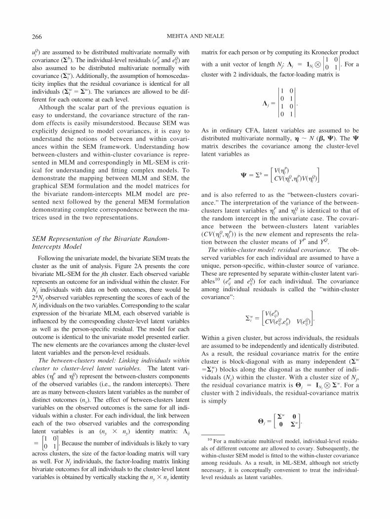
Figure 2. A: Bivariate random-intercepts model represented as a restricted confirmatory factor analysismodel. Observed scores for the multivariate outcome P and Q for all individuals (i) within cluster (j) loadon the corresponding between-level latent factors (�j

P and �jQ). �b is the covariance among the between

latent factors. Within-cluster residuals (eijP and eij

Q) for each individual are represented by correspondinglatent variables. �w is the covariance among the within-latent factors. The fixed-effects vector � (i.e.,means of the cluster-level latent variables) is represented as regression paths from a triangle representingconstant 1 for all individuals. Dashed line indicates the observed scores of individuals not depicted in thefigure. B: Succinct representation of the bivariate random-intercepts model. The figure represents themodel for a single individual (i) nested in cluster (j). The observed and latent variables as well asobserved residuals include person and cluster subscripts, indicating that the level of each variableinterpretation of parameters is identical to that in Figure 2A.


by maximizing the same likelihood. Finally, it is important tonote that the size of the factor-loading and residual-covariancematrix varies across clusters, depending on the number ofindividuals present in the cluster. As a result, unlike conven-tional SEM models, these matrices have a cluster subscript.More generally, in order to correctly identify the level of agiven variable, path diagrams also retain appropriatesubscripts.

MEM Formulation of the Bivariate Random-Intercepts Model

The MLM equations for the two outcomes can be com-bined into a single equation as

YijV � Dij

PP � DijQQ � Dij

PuijP � Dij

QuijQ � eij

V , (14)

where the multivariate outcomes are identified by defining twodummy variables DP and DQ for each individual, such thatDij

P � 1 and DijQ � 0, if the given row of observations for

individual i contains YP and DijP � 0 and Dij

Q � 1, if the givenrow of observation contains YQ. The dummy variables DP andDQ serve to select appropriate fixed and random effects foreach outcome variable. 11 The individual residual (eij

V) contin-ues to have a variable superscript. For two outcome variablesYP and YQ, the above equation for two clusters each with twoindividuals can be written as

Y � �Y11

P

Y11Q

Y21P

Y21Q

Y12P

Y12Q

Y22P

Y22Q

� � �1 00 11 00 11 00 11 00 1

�� P

Q � � �1 00 1

01 00 1

1 0

00 11 00 1

�� u1P

u1Q

u2P

u2Q�

� �e11

P

e11Q

e21P

e21Q

e12P

e12Q

e22P

e22Q

� . (15)

Note that Equation 15 links the unobserved person andcluster-level random effects for all individuals with theirrespective observed scores. The SEM model in contrastrepresents a single generic cluster. This equation corre-sponds to the following general MEM formulation:

y � X� � Zu � e, (16)

where y is a vector of the dependent variable, X is thematrix of independent predictors, � is the unknown vector

of regression parameters or the fixed effects coefficients, Zis a known design matrix used to specify the dependencystructure of the observations, u is the vector of unobservedrandom effects coefficients, and e is the unobserved vectorof random errors. The MEM explicitly incorporates randomeffects (u), effectively allowing nonindependent errors. Therandom effects (i.e., u and e) are assumed to be distributednormally and independently:

E�ue � � �0

0� and var �ue � � �G 0

0 R�.

The fixed-effects design matrix: The X matrix. With twooutcome variables, the fixed-effects vector has two elements(P and Q) and the corresponding X matrix has two col-umns containing the two dummy variables (DP and DQ). Fora given individual i with observations on both YP and YQ,

the Xij submatrix is �1 00 1� and is identical to the �ij

submatrix for a given individual. Not surprisingly, the Xj

submatrix for cluster j is identical to the cluster-level factor-loading matrix (Xj � �j).

The random-effects design matrix: The Z matrix. The Zmatrix in the bivariate case links the random effects (uj

P anduj

Q) for a given cluster j to appropriate rows of observations(YP or YQ) for all individuals in that cluster. In SEM, thislink matrix for a generic cluster j was defined by thefactor-loading matrix. In MEM, however, the link must beexplicitly defined between every cluster-level random vari-able and every individual observed score. As a result, thenumber of columns in Z equals the number of clusters timesthe number of outcome variables (Nj * ny). With two out-come variables and two clusters, there are a total of fourrandom effects. Hence, the Z matrix has four columns: thefirst two columns link the two random effects (u1

P and u1Q) for

Cluster 1 with the first four rows of observations, and thelast two columns link the two random effects (u2

P and u2Q) for

Cluster 2 with the last four rows of observations. Hence, theZ matrix has as many nonzero blocks as the number ofclusters. For each cluster, the Z matrix has a nonzero blockfor observations from that cluster. Each of these blockscontains the values of the two dummy variables (DP andDQ) for individuals within that cluster. In the parlance ofMEMs, the effects of the two dummy variables are assumedto be random at the cluster level. Note that the Zj submatrixfor any cluster j has two columns for the random effect ofeach outcome variable and is identical to the correspondingSEM factor-loading matrix j � Zj � Xj. Note that both Xj

and Zj submatrices are equal to the factor-loading matrix j.

11 Equation 14 or Equation 15 do not appear to have an “inter-cept” term. This is because we now have two outcomes andtherefore need an intercept term for each outcome. The grandmeans of the two dummy variables or their fixed effects representoutcome specific intercepts.

268 MEHTA AND NEALE

This is because, in SEM, the factor-loading matrix links thelatent variable (�) to the observed variables for each clus-ters: Yj � j�j. However, �j � � uj, hence Yj � j (� uj) � j� juj. In other words, at the cluster level, thefactor-loading matrix serves as the fixed-effects design ma-trix (Xj), as well as the random-effects design matrix (Zj).

We have shown the correspondence between SEM andMEM for all matrices except the latent factor and residualcovariance (i.e., the within- and between-clusters covari-ances). Recall that in SEM, the model is defined for a singlegeneric cluster j, whereas in MEM, the model is defined forall clusters and individuals. Hence, the covariance matricesfor the cluster-level random effects and individual-levelresiduals must be defined for all n clusters and for all Nindividuals. These covariances are specified as the G and Rmatrices, respectively.

Covariance among cluster-level random effects: The Gmatrix. Continuing with the bivariate example, for n clus-ters there are 2*n cluster-level random effects. Hence, thesize of the covariance matrix among u is (2n � 2n). For agiven cluster, the between-clusters covariance is �b. This isobviously identical to the between-clusters covariance inSEM (i.e., �). Clusters are assumed to be sampled ran-domly from the population of all clusters, leading to theassumption of independently and identically distributed ran-dom effects (uj

P and ujQ). As a result, across-clusters covari-

ance among the random effects is zero (CV�uk, uj� � 0),leading to a block-diagonal G matrix. The G matrix has asmany symmetric blocks as the number of clusters, witheach block equal to the between-clusters covariance ma-trix (�b). With two clusters, the G matrix has two sym-metric blocks:

G � � �b 00 �b . (17)

In general, with a total of n clusters, the G matrix is G� In � �b, where In is an (n � n) identity matrix. Note thatthe cluster-level submatrix of G is identical to the SEMlatent variable covariance matrix (�).

Covariance among individual residuals: The R matrix.For a total sample size of N, there are 2*N individual-levelresiduals. Hence, the size of the residual covariance matrixis (2N � 2N). For a given individual, the within-clustercovariance (eij

P and eijQ) is �w. Within clusters, individuals

are assumed to be sampled randomly, leading to the as-sumption of independently and identically distributed resid-uals. As a result, residual covariance across individuals iszero (CV�emj, enj� � 0), leading to a block-diagonal Rmatrix. The R matrix has as many symmetric blocks as thetotal sample size (N), with each block equal to the withincovariance (�w). With two clusters and two individualswithin each cluster, the R matrix has four symmetric blocks:

R � �w 0

�w

�w

0 �w�.

In general, for a sample size of N, the R matrix can besuccinctly represented as R � IN � �w where IN is an(N � N) identity matrix. The within-cluster submatrix of Ris identical to SEM residual covariance matrix (�).

Likelihood Equations in SEM and MEM

Given that SEM and MEM define the model at the levelof clusters and the entire sample data vector, respectively,the corresponding likelihoods are also computed at thecluster and sample level, respectively. For the multivariateMEM, the mean vector is

M � X�,

and the covariance matrix among all observations is

V � ZGZ� R.

The likelihood of a given vector of observations y is

�2LogL � K � log|V| � �y � M��V�1�y � M�,

where K � N*log(2�). For the corresponding SEM modelat the cluster level, the cluster-level means and covarianceare

uj � �j� and �j � �j � �j� �j. (18)

The likelihood of a vector of observations for cluster j, yj is

�2LogLj � Kj � log|�j| � �yi � �j��j�1�yj � �j�,

where Kj � Nj*log�2��. Because the clusters are assumedto be sampled independently, the log likelihood for theentire sample can be obtained as the sum of cluster �2LogLj

across all n clusters: �2LogL��j�1n (�2LogLj). In other

words, the two likelihoods are identical. Note that in prac-tice, all mixed-effects modeling software packages recog-nize the block diagonal structure of the G matrix andcompute the likelihood using the second approach (Verbeke& Molenberghs, 2000). Hence, although the model repre-sentation stacks data for all individuals and variables into asingle column, and the model specification requires theinclusion of “dummy” intercepts for accommodating themultivariate data structure, the specification and computa-tion of the likelihood is done in a computationally efficientfashion. By corollary, the data-handling capability for spec-ifying models with nested data structures and full-informa-tion likelihood in SEM is in and of itself inadequate forefficient estimation. Efficient algorithms similar to thoseused in MEM for computing the likelihood at the clusterlevel are necessary in ML-SEM (du Toit & du Toit, 2003).


Graphical Representation of Bivariate Random-Intercepts Model

The bivariate random-intercepts model can also be rep-resented succinctly using the notion of exchangeability. Asin the case of the univariate random-intercepts model, clus-ters and individuals are both considered exchangeable.Hence, it is necessary to represent the model for a singlecluster (j) and a single individual (i) within that cluster.However, the two outcome variables (YP and YQ) are notexchangeable. Therefore, we need to represent the twovariables and their between and within covariances sepa-rately. Figure 2B succinctly depicts a bivariate random-intercepts model. The figure shows all model parametersand is an accurate representation of a bivariate random-intercepts model. As in the univariate case, it is assumedthat (a) clusters and individuals are sampled randomly andindependently; (b) multiple observed repeated measures forall individuals belonging to cluster j load onto the commoncorresponding between-clusters variables; (c) conditionalon the common between-clusters latent factors, the residualsfor each outcome (eij

P and eijQ) are independent across indi-

viduals; and (d) within-cluster covariance among residuals(�w) is equal for all individuals.

Multilevel Measurement and Structural Models

Once the within and between-clusters covariances havebeen estimated, separate model-based restrictions may beimposed on these covariances to estimate within- and be-tween-clusters measurement and structural parameters (seealso Goldstein & Browne, 2002; Heck, 2001; Kaplan &Elliot, 1997; Snijders & Bosker, 1999). This is accom-plished by defining additional within and between latentvariables that impose restrictions on the core within- andbetween-clusters covariance matrices (Longford & Muthen,1992; Muthen, 1991). For example, we can fit a measure-ment model at the between and within cluster level. Thisinvolves defining measurement model at the two levels andimposing constraints on the corresponding matrices:

�b � �b�b�b� � �b and �w � �w�w�w� � �w. (19)

The covariance for the entire cluster is

�j � �1Nj� Iny

��b�1Nj� Iny

�� INj� �w.

The above equations define conventional measurementmodels at the within- and between-clusters levels, respec-tively. The measurement models may be different at the twolevels. The parameters of the new measurement or structuralmodel may be estimated by maximizing the same likelihoodfunction. So long as the model is identified, 12 any mean-ingful SEM may be used for imposing restrictions on thebetween-clusters and within-cluster covariances. The differ-ence in �2LogL for the unconstrained model and the con-

strained model may be used to evaluate the appropriatenessof the restrictions imposed by the within- and between-clusters SEMs.

The multivariate, multilevel latent variable model im-plied by the previous specification uses the general-specificfactor model as a template as opposed to the hierarchicalfactor model (Gustafsson, 2002; Gustafsson & Balke,1993). The cluster-level specification represents the generalpart of the model, whereas the individual-level model cor-responds to the specific part of the model. From this per-spective, the base model (i.e., the multivariate MEM) alsouses the general-specific factor model template. Bauer(2003) and Curran (2003) used a conceptually appealing butrestrictive alternative, the hierarchical factor model as atemplate for conceptualizing multilevel latent variable mod-els. However, the hierarchical model specification implies aspecific set of constraints on the less restrictive general-specific model. The first restriction is the restriction im-posed by the within- and between-clusters factor models onthe within- and between-clusters covariances (Equation 19).The second set of restrictions is related to (a) the assumptionof invariant factor loadings across levels and (b) the as-sumption of zero variances of observed indicators at thecluster level. These restrictions are illustrated next in thecontext of an empirical example. It should be noted that thenotion of hierarchical factor models can also be used as themeasurement model for the clustered data (see Harnqvist,Gustafsson, Muthen, & Nelson, 1994).

Multilevel CFA: Empirical Example

We illustrate estimation of within- and between-clusterscovariances as well as fitting a measurement model at thetwo levels with an example from reading research. The datacome from a larger longitudinal study of early readingdevelopment involving 1,052 third graders nested within115 classrooms (Mehta, Foorman, Branum-Martin, & Tay-lor, 2005). The sample was primarily African American(94.58%) with Hispanics being the second largest group(4.66%). These data come from end-of-the-year assessmentof literacy skills and include the following broad measuresof literacy: phonemic awareness (PA), word reading (WR),spelling (S), vocabulary (V), and writing (WT). The detailsof the psychometric properties of these measures can befound elsewhere (Foorman et al., 2003). We consider thepossibility that these diverse measures of English literacyare indicators of a single factor, both at the individual and atthe classroom level. Initial univariate and multivariateMEMs were fitted using SAS Proc Mixed, and the ML-CFA

12 The multivariate MEM is identified so long as there areenough clusters to meaningfully estimate covariances at the be-tween-clusters level and enough individuals to estimate within-cluster covariance. Conventional rules of identification apply forfitting SEM models at each level.

270 MEHTA AND NEALE

model was fitted using Mplus (Version 3; Muthen & Mu-then, 2004).

Univariate Random-Intercepts Model

As a first step, a univariate random-intercepts model wasfitted to the data, with classroom as the Level 2 nesting unit(see Table 1). The between-classroom variability was sig-nificant for each of the five measures with ICCs (proportionof variance attributable to between-clusters variability)ranging from 0.10 to 0.24. The means of each measure arealso reported in Table 1. Grand means are not particularlyinteresting in a single-group model and are ignored insubsequent analyses. It is obvious that univariate analysesdo not provide any information regarding covariance amongoutcomes at the within- and between-clusters levels.

Multivariate Random-Intercepts Model

A multivariate random-intercepts model (see Figure 3)was fitted in Proc Mixed to obtain between-clusters (�b)and within-cluster (�w) covariance among the outcomemeasures. Table 2 presents these between-clusters and with-in-cluster covariances (below the diagonal) along with thecorresponding correlations (above the diagonal). Note thatthe estimated within- and between-clusters variances (diag-onal elements) were almost identical to those reported inTable 1 for the univariate random-intercepts model. Thecorrelations among the outcome variables are different atthe two levels (see Figure 3). Eight out of 10 correlations atthe between-clusters level are larger than the correspondingwithin-cluster correlations. The patterns of within- and be-tween-clusters correlations are consistent with a unidimen-sional model at each level. A single-factor model assertsthat a single latent factor explains the between-clusters (�b)and within-cluster (�w) covariances; that is, conditional onthe latent factors at each level, the within- and between-clusters residuals are independent.

Multilevel CFA

Table 3 presents the unstandardized parameter estimatesfor the ML-CFA fitted in Mplus 3.11. All five observedvariables were allowed to load onto a single literacy factor

at both the within- and between-clusters level. The latentfactor scales at each level were identified by fixing the WRfactor loading to 1.0. The remaining factor loadings, latentfactor variances, and residual variances were freely esti-mated at both levels. Measurement intercepts were esti-mated for all five outcome variables, and the mean of thebetween-clusters literacy factor was fixed to 0.0. Because norestrictions were imposed on the mean structure, the esti-mated intercepts were almost identical to the correspondinggrand means in the univariate MEM. Standardized param-eter estimates for the ML-CFA are presented in Figure 4.

Mplus reports within- and between-clusters estimated

Table 1Univariate Random-Intercepts Mixed-Effects Models: Fixed and Random Effects

Outcome Grand mean SEBetween-clusters

variance SEWithin-cluster

variance SE ICC

Spelling 91.38 0.65 29.23 6.39 158.99 7.41 0.15Word reading 2.27 0.04 0.08 0.02 0.70 0.03 0.10Phonemic awareness 0.93 0.03 0.05 0.01 0.21 0.01 0.18Writing �0.08 0.05a 0.18 0.03 0.55 0.03 0.24Vocabulary 78.67 0.70 28.87 7.47 229.24 10.79 0.11

Note. ICC � intraclass correlation.a Not significant.

Figure 3. Multivariate random-intercepts model of literacy. Theobserved variables (uppercase) include person and cluster sub-scripts. Individual-level residuals (eij) for each outcome are rep-resented as latent variables. Superscripts b and w indicate between-clusters and within-cluster latent variables (lower case). Between-level latent variables have a cluster subscript, whereas the within-level latent variables have both individual and cluster subscripts.The five outcome variables are spelling (S), word reading (WR),phonemic awareness (PA), writing (WT), and Vocabulary (V). Thegrand means of the between-level latent variables are not includedfor clarity. Numbers represent correlations among latent variables.


sample statistics. These estimates are obtained by fitting anunrestricted model (referred to as the H1 model). The H1model is in fact identical to the multivariate MEM presentedpreviously (see Figure 3). Explicitly fitting MEM clarifiesthe source and the meaning of the sample statistics reportedby Mplus. Mplus parameter estimates and the fit statisticsfor the H1 model were identical to those reported by ProcMixed for the corresponding multivariate random-interceptsmodel (see Table 2).

The Mplus log likelihood for the H1 model was�10,753.615. The corresponding Proc Mixed �2LL for themultivariate MEM was 21,507.2 ( � �2*�10,753.615).The Mplus log likelihood for the restricted (H0) model was10,761.576. Given certain regularity conditions, the differ-ence in �2LL between the H0 and H1 model is distributedas a chi-square with degrees of freedom equal to the differ-ence in the number of parameters estimated by the twomodels. In this case, the overall fit statistic was �10

2 � 15.92(p � .10), suggesting that the restriction imposed by theML-CFA model on the within- and between-clusters covari-ances did not result in a worse fitting model. Standardizedroot mean squared residual for the between and withinmodels were 0.043 and 0.019, respectively, suggesting thatthe multilevel model did an adequate job in reproducingcovariances at both levels.

The estimated variance of the latent literacy factor at thewithin- and between-clusters level was 0.52 and 0.10, re-spectively. However, in the absence of a common scale, themagnitude of these variances is not directly comparable.The issue of establishing common across-level scale isdiscussed in the next section. The proportion of varianceexplained by the latent literacy factor at the within levelranged from .16 to .72. The corresponding proportions at the

between level ranged from .15 to .96. The relatively lowproportion of variance explained at the within level suggeststhat after controlling for classroom variability in literacy,there is considerable heterogeneity in the within-individualvariability in literacy. At the between level, PA and WT hadthe lowest R2. It is generally acknowledged that PA may bea less important indicator of literacy beyond second grade.This could explain the low R2 for PA at both within- andbetween-clusters level. On the other hand, low R2 for WT at

Table 2Multivariate Random-Intercepts Mixed-Effects Model: Fixed and Random Effects

Outcome Spelling Word reading Phonemic awareness Writing Vocabulary

Grand mean 91.29 (0.65) 2.31 (0.04) 0.95 (0.03) �0.10 (0.05) 78.57 (0.70)

Between-clusters covariance/correlation (Gj)a,b

Spelling 29.26 (6.41) 0.86 0.41 0.58 0.78Word reading 1.49 (0.36) 0.10 (0.02) 0.36 0.57 0.92Phonemic awareness 0.51 (0.20) 0.03 (0.01) 0.05 (0.01) 0.10 0.36Writing 1.31 (0.37) 0.08 (0.02) 0.01 (0.01) 0.18 (0.03) 0.53Vocabulary 22.82 (5.71) 1.60 (0.36) 0.45 (0.21) 1.21 (0.38) 29.33 (7.47)

Within-cluster covariance/correlation (Rij)a,b

Spelling 158.42 (7.36) 0.68 0.32 0.51 0.31Word reading 7.28 (0.43) 0.72 (0.03) 0.40 0.53 0.33Phonemic awareness 1.85 (0.21) 0.16 (0.01) 0.21 (0.01) 0.25 0.18Writing 4.83 (0.35) 0.33 (0.02) 0.09 (0.01) 0.55 (0.03) 0.31Vocabulary 59.74 (6.63) 4.27 (0.46) 1.23 (0.25) 3.47 (0.40) 228.69 (10.73)

Note. Numbers in parentheses represent the standard error. �2LL for the model is 21,507.200a Covariances are presented below the diagonal, and correlations are above the diagonal.b Diagonals elements are the variances.

Table 3Multilevel Confirmatory Factor Analysis: UnstandardizedParameter Estimates

Measure Factor loading Residual variance R2

Within clustera

Spelling 13.91 (0.65) 57.32 (4.55) 0.64Word reading 1.00 0.20 (0.02) 0.72Phonemic awareness 0.28 (0.02) 0.17 (0.01) 0.19Writing 0.65 (0.04) 0.33 (0.02) 0.40Vocabulary 8.47 (0.75) 191.20 (9.33) 0.16

Between clustersb

Spelling 15.16 (1.91) 6.28 (2.63) 0.78Word reading 1.00 0.00 (0.01)c 0.96Phonemic awareness 0.28 (0.10) 0.04 (0.01) 0.15Writing 0.81 (0.17) 0.11 (0.02) 0.36Vocabulary 15.72 (2.50) 5.02 (4.40) 0.83

Note. Numbers in parentheses represent the standard error. �2LL for themodel was 21,523.152.a Variance of the literacy factor at the within level was 0.52(0.04). b Variance of the literacy factor at the between level was 0.10(0.02). c Residual variance for word reading at the between level waspractically estimated at zero.

272 MEHTA AND NEALE

the between level may indicate that there may be some otherfactor influencing classroom level variability in WT.

Random Intercepts for a Latent Variable

So far we have described latent literacy factor at both thewithin- and between-clusters level. This raises two relatedquestions: (a) If there can be random intercepts (i.e., vari-ability in the cluster means for individual-level observedvariables), can we have a random intercept for the individ-ual-level literacy factor? (b) Alternatively, does the cluster-level literacy factor mean the same thing as the literacyfactor at the individual level? Technically these are ques-tions of across-level invariance of the measurement model.

Consider a two-level measurement model with p observedvariables and q latent variables at each level. Each of the pobserved variables may be expressed in terms of within- andbetween-clusters deviations:

YijP � P � yj

P�b� � yijP�w�.

These within- and between-clusters deviations serve as in-dicators of qth within and between latent variables:

yijP�w� � �pq

�w��ijQ�w� � eij

P�w� and yjP�b� � �pq

�b��jQ�b� � �j

P�b�.

If the factor loadings are invariant across levels ��pq�b�

� �pq�w� � �pq�, then the above expression may be simpli-

fied as

YijP � P � �pq�j

Q�b� � �jP�b� � �pq�ij

Q�w� � eijP�w� � P

� �pq��ijQ�w� � �j

Q�b�� jP�b� � eij

P�w�

� P � �pq�ijQ � �j

P�b� � eijP�w�

where �ijQ is an individual-level latent variable that is itself

composed of within- and between-clusters deviations: �ijQ

� �ijQ�w� � �j

Q�b�. In other words, we now have an indi-vidual-level latent variable with a random intercept at thebetween-clusters level. Conceptually, invariance of across-level factor loading equates the scales of the latent commonfactor across levels, thus making latent factor variances tobe directly comparable. Also note that the observed indica-tor continues to have variability at the between level (�j

P�b�).This is the residual for the second-level factor model.

For the literacy data, the hypothesized model with invari-ant factor loadings is presented in Figure 5. The literacyfactor at the individual level now has a cluster-level randomintercept. In addition, the observed variables continue tohave cluster-level random intercepts. These are actually, theresidual variances for the between-level random intercepts.As such, the random intercepts for Level 2 observed resid-uals are independent of the between latent literacy factor.The Mplus log likelihood for the model with invariantacross-level factor loadings was �10,753.615. The differ-ence in �2LL between the model with and without invariantfactor loadings was �4

2 � 8.618 (p � .071), indicating thatthe hypothesis of invariant factor loadings cannot be re-jected. The parameter estimates of the model with invariantfactor loadings are presented in Table 4 and are generallyvery similar to the unconstrained model. Invariant factorloadings make common-factor variances to be directly com-parable across levels. The variance of the random interceptfor the literacy factor was 0.111, and the correspondingresidual within-cluster variance was 0.507. The proportionof variance in the individual-level literacy factor explainedby its random intercept or ICC for the latent literacy factorwas .18.

The model presented in Figure 4 uses the general-specificfactor model as a template, with the between-level modelrepresenting the general factor, and factor models for eachindividual representing the specific factors. In contrast,model in Figure 5 is analogous to the hierarchical factormodel, in which latent variables at the individual-level (i.e.,the first-order factors) define the latent factor at the higherlevel. However, note that individual observed indicators

Figure 4. Multilevel confirmatory factor analytic model of liter-acy: completely standardized solution. The between- and within-level latent variables are allowed to load onto the correspondingbetween- and within-level literacy factors (lit). The five outcomevariables are spelling (S), word reading (WR), phonemic aware-ness (PA), writing (WT), and Vocabulary (V). Note that the factormodel includes residual variances at each level. The measurementintercepts of the between-level residuals are not included forclarity.


continue to retain variability at the higher level (�jP�b�). In

summary, invariance of across-level factor loadings in thegeneral-specific model and zero variability for the observedindicators at the second level are necessary prerequisites forthe use of the parsimonious hierarchical factor model(Bauer, 2003; Curran, 2003).

Random Slopes in SEM and MLM

The notion of random slopes is novel in general SEM forclustered data. Hence, we present this idea conceptuallywithin its native MLM framework and demonstrate how therandom slope may be represented as a latent variable withinthe familiar CFA model. The random-intercepts model canbe extended to include the random effect of an individualpredictor (Xij):

Yij � �1j1 � �2jXij � eij, (20)

where �2j is the effect of X on Y for the jth cluster, and �1j

is the intercept (i.e., the level of Yij when Xij � 0). Thepresence of subscript j in �2j indicates that the regressioncoefficient is assumed to vary across clusters, hence theterm random slopes. The random regression coefficients canbe expressed in deviation form as

�1j � 1 � u1j and �2j � 2 � u2j, (21A & 21B)

Figure 5. Random intercept for a latent variable: multilevel confirmatory factor analytic modelwith invariant across-level factor loadings. The factor loadings and residual variances at eachlevel are standardized estimates. Numbers in italics are the standardized between-factorloadings. The variance of the literacy factor (lit; in bold) at each level is unstandardized. Thefive outcome variables are spelling (S), word reading (WR), phonemic awareness (PA), writing(WT), and Vocabulary (V). Note that the unstandardized factor loadings are invariant as shownin Table 4.

Table 4ML-CFA With Invariant Across-Level Factor Loadings:Unstandardized Parameter Estimates

Measure Factor loading

Residualvariance/standard

deviation R2

Within clustera

Spelling 14.16 (0.58) 56.74 (4.37) 0.64Word reading 1.00 0.20 (0.02) 0.71Phonemic awareness 0.28 (0.02) 0.17 (0.01) 0.19Writing 0.67 (0.04) 0.33 (0.02) 0.41Vocabulary 9.49 (0.69) 190.43 (9.35) 0.19

Between clustersb,c

Spelling 14.16 (0.58) 2.58 (0.45) 0.77Word reading 1.00 0.00 (0.17)c 1.00Phonemic awareness 0.28 (0.02) 0.21 (0.02) 0.17Writing 0.67 (0.04) 0.34 (0.03) 0.30Vocabulary 9.49 (0.69) 2.977 (0.711) 0.53

Note. Numbers in parentheses represent the standard error. �2LL for themodel was 21,531.800.a Variance of the literacy factor at the within level was 0.51(0.04). b Variance of the literacy factor at the between level was 0.11(0.02). c At the between-level, residual standard deviations were esti-mated to avoid negative residuals. d Residual variance for word readingat the between level was practically estimated at zero. ML � multilevel;CFA � confirmatory factor analysis.

274 MEHTA AND NEALE

where 1 and 2 are the mean intercepts and slopes, respec-tively, and u1j and u2j are the corresponding cluster devia-tions. Note that the intercept is defined at Xij � 0. If Xij iscentered at the grand mean, then 1 and u1j are defined atthe grand mean of Xij.

Formulating Random Slope as an SEM LatentVariable: The Notion of a Definition Variable

For the random-intercept model, the observed variables(Yij) were the scores for an individual i nested within class-room j. The latent variable (�1j) represented the randomintercept. Because individuals within classrooms are inter-changeable, the factor loading (�i,1) for each individual wasfixed to 1.0. Similarly, intercluster variability in the effect ofX on Y (�2j) may be represented as a random variable. To doso, the factor loadings for �2j must be fixed to the observedvalue of Xij for each individual (�i,2 � Xij), which may infact be different for every individual in the sample. Untilvery recently, most popular SEM software did not supportany mechanism for fixing model parameters to an individ-ual’s data values. Currently, Mx (Neale et al., 2004) andMplus13 (Muthen & Muthen, 2004) offer such a capability,and the variable that is used for fixing model parameters iscalled a “definition variable.”

Graphical representation of a random-slopes model.Figure 6A presents a CFA formulation of the random-slopesmodel. Xij is used as a definition variable in which individ-ual-specific values of Xij are used to fix model parameters(i.e., the slope factor loadings of Yij on �2j). Definitionvariables are represented by placing the variable (Xij) insidea diamond symbol ({). As in the case of a random-inter-cepts model, because individuals are assumed to be ex-changeable, it is necessary to represent the model for asingle individual only. Figure 6B illustrates a CFA formu-lation of the random-slopes model using the succinct graph-ical representation introduced earlier. Two extensions to theRAM notation (McArdle & Boker, 1990) are necessary forrepresenting a random-slopes model: (a) the inclusion ofindividual and cluster subscripts to incorporate multilevelinformation and (b) the use of diamonds to represent defi-nition variables.

An alternate graphical representation of a random-slopesmodel. Random slopes are graphically represented in asomewhat different fashion in Mplus (Figure 6C). Thisapproach does not use individual and cluster subscripts toindicate the level of each variable, instead the within andbetween parts of the model are represented by using explicitlabels and by a line separating the two models. The outcomevariable is assumed to have variability at the cluster level.The fact that the effect of Xij on Yij is random at the clusterlevel is represented by a dot on the line representing theregression effect of X on Y (in the within part of thediagram). Within the script, the corresponding random re-

gression is specified as: S | Y on X. The label of the randomeffect so defined (s) is placed next to the dot to indicate thename of the random variable at the cluster level. The ran-dom intercept at the between level is referred to by thevariable label of the dependent variable. The between partof the diagram has two latent variables y (intercept) and s(slope) for the two random effects.

We prefer the extended RAM notation for representingmultilevel SEM models for several reasons. First, the pathdiagram is a direct, complete, and mathematically accuraterepresentation of the underlying model, and may be used forrepresenting random slopes of any type at both levels (in-dividual and cluster), including random slopes in the con-text of longitudinal data with continuously varying values oftime and possibly time-varying covariates. Second, conven-tional rules of a path diagram may be used without anymodifications to derive the implied means and covariances.Third, the extended RAM notation reformulates the notionof random slopes into the familiar concept of a restrictedCFA model, yet the meaning of the diagram is readilyinterpretable in terms of both the multilevel random-slopesmodel and the restricted CFA model. For example, bothintercept and slope factors are defined as conventional latentvariables, with factor loadings fixed to 1.0 and the person-specific Xij, respectively. Fourth, the diagram makes anexplicit distinction between a modeled dependent variable(Yij) and an exogenous observed variable Xij used as adefinition variable.

Correspondence Between the SEM and MEMFormulation of Random Slopes

It is clear from Figures 6A and 6B that the random-slopesmodel can be represented as a cluster-level restricted CFAmodel in which the factor loadings for the slope are fixed toindividual specific values of the predictors Xij. For cluster jwith three individuals, the factor-loading matrix is

�j � � 1 X1j

1 X2j

1 X3j

�.

In general, for a cluster with Nj individuals, the factor-loading matrix is �j � �1Nj

|Xj� where 1Njis a unit vector, Xj

is the predictor vector for all individuals in cluster j, and |represents horizontal concatenation of the two column vec-tors. The two latent factors (�1j and �2j) represent therandom intercept and random slope, respectively. The latentfactor means represent the fixed effects:

��1

2�,

13 Mplus does not use the term definition variable, althoughsuch a functionality is implicitly available to a certain extent.


and the latent factor covariances represent the cluster-levelcovariance between the intercept and slope factors:

�j � �V�u1j�CV�u2j,u1j� V�u2j�

�.

Finally, the residual covariance matrix contains variances ofresiduals for all individuals in cluster j.

�j � �w2

w2

w2�.

Because individuals within a cluster are assumed to beinterchangeable, residual variances are equal. For a clusterwith Nj individuals, the residual covariance matrix is� � INj

� w2 , where INj

is an identity matrix, and w2 is the

common residual variance. As in the case of the random-intercepts model, the above matrices for the CFA formula-tion of the random-slopes model correspond to matrices ofthe corresponding MEM matrices: the factor-loading matrix(�j) corresponds to Xj and Zj matrices, the factor covari-ance matrix (�) corresponds to the Gj matrix, the residual-covariance matrix (�j) corresponds to the Rj matrix, and thelatent factor mean vector is identical to the fixed-effectsvector (�).

Model-Implied Covariance: Person-SpecificCovariances

Given the previous formulation of a random-slopes modelas a CFA model, the model-implied covariances and meansare identical to the corresponding equations for the CFAformulation of the general MEM. Although the restrictedCFA is used for modeling both random-intercepts and ran-dom-slopes model, the model-implied covariance matrixfor the random-slopes model is very different from thatfor the random-intercepts model. This difference is due tothe presence of Xij as a definition variable and necessi-tates certain modifications to the underlying softwarebefore FIML estimation can be used to fit models withrandom slopes.

Recall that the model-implied covariance matrix for therandom-intercepts model has a very simple structure withwithin-cluster covariance among any two Yij equal to thevariance of the random intercept, and the variance for eachindividual is equal to the sum of the between-clusters andwithin-cluster variances. This is no longer true for therandom-slopes model. The variance of Ymj for individual mis

regression of Y on X is random at the between level. The within-level dependent variable is assumed to be random at the betweenlevel, which now becomes the random intercept. Between-levelrandom intercept and slope are represented as latent variables.

Figure 6. A: Univariate random-slopes model represented as arestricted CFA model. Observed scores of all individuals (Yij) incluster j are allowed to load onto two latent factors: intercept (�1j)and slope (�2j). The factor loadings for all observed variables onthe intercept factor are fixed to 1.0. The factor loading for eachindividual on the slope factor is fixed to individual’s observedscore on Xij (definition variables). Definition variables are repre-sented by a diamond symbol. Dashed line indicates scores ofindividuals not included in the figure. The within-cluster residualvariance is assumed to be equal for all individuals (�). B: Succinctrepresentation of univariate random-intercepts model. The figurerepresents the model for a single generic individual (i) nested incluster (j). The observed variable includes both person (i) andgroup (j) subscripts, whereas the cluster-level latent intercept andslope factors include the cluster subscript. Definition variables (Xij)are represented by a diamond symbol. All model parameters areexplicitly represented in the figure. C: Mplus representation of arandom-slope model. Within and between levels are separated bya dashed line. A dot on the within-regression indicates that the

276 MEHTA AND NEALE

V�Ymj� � V�I� � 2Xmj*C�S,I� � �Xmj�2V�S� � V�yw�,

and the covariance between scores of any two individualsYmj and Ynj is

C�Ymj,Ynj� � V�I� � V�S�XmjXnj � C�S,I�Xmj � C�S,I�Xnj.

It is clear that for the random-slopes model, the co-variance among individuals within a cluster is a functionof person-specific values of Xij. More simply, there is nosingle covariance matrix for the entire sample as in thecase of conventional SEM. Instead, in order to fit arandom-slopes model as an SEM model, covariancesmust be modeled as a function of predictors. As a result,conventional sample means- and covariance-based MLestimation is not suitable for modeling a random-slopesmodel. In principle, FIML estimation allows the covari-ance for each unit (in this case, the cluster) to be modeledas a function of an individual’s values on predictors (inthis case, Xij). To do so, a special data-handling mecha-nism is needed that allows model parameters to be fixedto person-specific data values. Although FIML estimationhas been available in popular SEM software for sometime, the value of modeling covariances as a function ofobserved data values has not been widely recognized andhence incorporation of random slopes within SEM soft-ware has been slow in coming.

Random Slopes in ML-SEM: Empirical Example

We now illustrate a bivariate random-slopes modelfrom a ML-SEM perspective. The data used in this ex-ample come from a bilingual (Spanish and English) re-search study involving 1,418 kindergartners clusteredwithin 134 classrooms. Students were in one of twodifferent types of language instructional programs: (a)immersion with an exclusive focus on instruction inEnglish and (b) nonimmersion, including various levelsand types of bilingual instruction. The dependent vari-ables of interest include reading ability in English (RAE)and Spanish (RAS), and the independent variable is thelevel of blending words/Spanish (BWS). Blending words/Spanish is a component of phonological awareness andinvolves the ability to blend separate sounds to produce aword. It is hypothesized that the effect of BWS on RAEand RAS will vary across classrooms. In addition, thecluster-level variable, language instructional program, ishypothesized to predict the level of classroom RAE andRAS as well as the classroom variability in the effect ofBWS on RAE and RAS, respectively. Within classrooms,the RAE and RAS residuals are expected to be correlated.

Table 5 and Figure 7 present the hypothesized modelalong with the parameter estimates. For each outcome (RAEand RAS), there are two classroom-level latent variables: (a)the random-intercept or the average level of the outcome at

Table 5Bivariate Random-Slopes Model: Parameter Estimates

Between-clusters model

English Spanish

English intercept English slope Spanish intercept Spanish slope

Latent variable covarianceb

Random factorEnglish intercept 0.515 (.108) .355 �.416 �.498English slope 0.018 (0.011) 0.005 (0.002) .210 .316Spanish intercept �0.242 (0.081) 0.012 (0.012) 0.656 (0.108) .607Spanish slope �0.016 (0.009) 0.001 (0.001) 0.022 (0.011) 0.002 (0.001)

Fixed effects

PredictorIntercept �0.251 (0.085) 0.195 (0.013) 0.119 (0.097) 0.211 (0.010)Immersion 1.332 (0.169) 0.049 (0.028) �1.234 (0.167) �0.076 (0.024)

Residuals

Within-cluster model(residual covarianceb)

English Spanish

English 1.593 (0.122) .565Spanish 0.800 (0.070) 1.259 (0.092)

Note. Correlations are above the diagonal. Model log likelihood � �4,350.045.a Within- and between-clusters covariances are conditional or residual covariance matrices.b Numbers in parentheses represent the standard error.


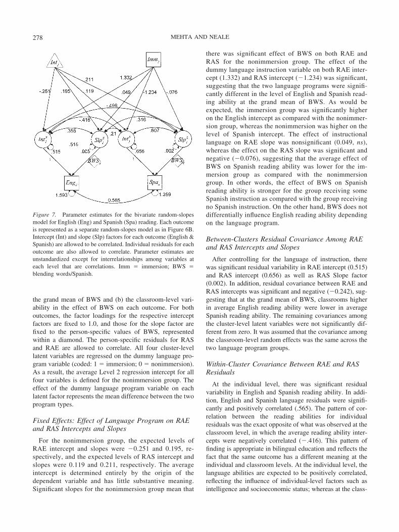
the grand mean of BWS and (b) the classroom-level vari-ability in the effect of BWS on each outcome. For bothoutcomes, the factor loadings for the respective interceptfactors are fixed to 1.0, and those for the slope factor arefixed to the person-specific values of BWS, representedwithin a diamond. The person-specific residuals for RASand RAE are allowed to correlate. All four cluster-levellatent variables are regressed on the dummy language pro-gram variable (coded: 1 � immersion; 0 � nonimmersion).As a result, the average Level 2 regression intercept for allfour variables is defined for the nonimmersion group. Theeffect of the dummy language program variable on eachlatent factor represents the mean difference between the twoprogram types.

Fixed Effects: Effect of Language Program on RAEand RAS Intercepts and Slopes

For the nonimmersion group, the expected levels ofRAE intercept and slopes were �0.251 and 0.195, re-spectively, and the expected levels of RAS intercept andslopes were 0.119 and 0.211, respectively. The averageintercept is determined entirely by the origin of thedependent variable and has little substantive meaning.Significant slopes for the nonimmersion group mean that

there was significant effect of BWS on both RAE andRAS for the nonimmersion group. The effect of thedummy language instruction variable on both RAE inter-cept (1.332) and RAS intercept (�1.234) was significant,suggesting that the two language programs were signifi-cantly different in the level of English and Spanish read-ing ability at the grand mean of BWS. As would beexpected, the immersion group was significantly higheron the English intercept as compared with the nonimmer-sion group, whereas the nonimmersion was higher on thelevel of Spanish intercept. The effect of instructionallanguage on RAE slope was nonsignificant (0.049, ns),whereas the effect on the RAS slope was significant andnegative (�0.076), suggesting that the average effect ofBWS on Spanish reading ability was lower for the im-mersion group as compared with the nonimmersiongroup. In other words, the effect of BWS on Spanishreading ability is stronger for the group receiving someSpanish instruction as compared with the group receivingno Spanish instruction. On the other hand, BWS does notdifferentially influence English reading ability dependingon the language program.

Between-Clusters Residual Covariance Among RAEand RAS Intercepts and Slopes

After controlling for the language of instruction, therewas significant residual variability in RAE intercept (0.515)and RAS intercept (0.656) as well as RAS Slope factor(0.002). In addition, residual covariance between RAE andRAS intercepts was significant and negative (�0.242), sug-gesting that at the grand mean of BWS, classrooms higherin average English reading ability were lower in averageSpanish reading ability. The remaining covariances amongthe cluster-level latent variables were not significantly dif-ferent from zero. It was assumed that the covariance amongthe classroom-level random effects was the same across thetwo language program groups.

Within-Cluster Covariance Between RAE and RASResiduals

At the individual level, there was significant residualvariability in English and Spanish reading ability. In addi-tion, English and Spanish language residuals were signifi-cantly and positively correlated (.565). The pattern of cor-relation between the reading abilities for individualresiduals was the exact opposite of what was observed at theclassroom level, in which the average reading ability inter-cepts were negatively correlated (�.416). This pattern offinding is appropriate in bilingual education and reflects thefact that the same outcome has a different meaning at theindividual and classroom levels. At the individual level, thelanguage abilities are expected to be positively correlated,reflecting the influence of individual-level factors such asintelligence and socioeconomic status; whereas at the class-

Figure 7. Parameter estimates for the bivariate random-slopesmodel for English (Eng) and Spanish (Spa) reading. Each outcomeis represented as a separate random-slopes model as in Figure 6B.Intercept (Int) and slope (Slp) factors for each outcome (English &Spanish) are allowed to be correlated. Individual residuals for eachoutcome are also allowed to correlate. Parameter estimates areunstandardized except for interrelationships among variables ateach level that are correlations. Imm � immersion; BWS �blending words/Spanish.

278 MEHTA AND NEALE

room level, the negative correlation between the averagelevels of reading ability reflects differences in the pattern ofEnglish and Spanish instruction across classrooms. Gener-ally speaking, in the current sample, classrooms with higherlevels of English instruction tended to have lower levels ofSpanish instruction, and vice versa, explaining the negativecorrelation between the two abilities at the classroom levels.

Random Slopes Versus Cross-Level Latent Variableby Observed Variable Interaction

The empirical example presented above for illustratingthe use of random slopes in SEM was rather trivial. How-ever, the latent variable approach to modeling random ef-fects offers an interesting alternative substantive interpreta-tion more in line with the latent variable modelingperspective. From a MEM perspective, the effect of BWSon RAS and RAE is assumed to vary randomly acrossclassrooms. This interpretation is implicit in the graphicalrepresentation used by Mplus (Figure 6C). From a latentvariable perspective, we have classroom-level latent vari-ables (random slope for RAS and RAE), perhaps indicativeof an unobserved classroom-level construct, whose effect ismoderated by the level of individual-level BWS. Both per-spectives are consistent with the underlying mathematicalmodel. However, the cross-level interaction between anobserved and a latent variable is closer in spirit to the latentvariable modeling perspective. This is clearly evident in thegraphical representation of the model using the extendedRAM notation (see Figure 7).

Discussion

The current article extended Mehta and West’s (2000)approach of fitting LGC models for continuous time to thegeneral case of ML-SEMs with random slopes. The articledemonstrates the equivalence of the general multivariateMEM and ML-SEM with definition variables. MEMs areconceptualized as a special case of the restricted CFAmodel. The article also provides an extended RAM notationfor graphical representation of ML-SEMs with randomslopes. The extended graphical notation is a concise andmathematically complete representation of the model aswell as its assumptions. The graphical notation should assistin conceptualizing complex ML-SEMs and also facilitatecommunication among researchers. The most importantquestion from a practitioner’s perspective is the following:How applicable are ML-SEM models for answering sub-stantive questions of interest? In addition, in applied set-tings, methodological issues regarding the estimation andevaluation of ML-SEMs are critical. These issues are high-lighted next.

Applicability of ML-SEM Models

MLM is generally thought of as multiple regression forclustered data. In the same way that SEM improves onmultiple regression, ML-SEM brings the advantages of la-tent variable modeling to MLM for clustered data. There-fore, ML-SEM models are well suited to the kinds ofquestions for which SEM is best known.

Multilevel measurement models. The multilevel mea-surement model is perhaps the most important class ofML-SEM application. It is possible to estimate individual-level measurement models using observed or latent individ-ual-level indicators. Similarly, it is possible to define clus-ter-level measurement models using the cluster-levelrandom intercepts for the individual-level variables as wellas cluster-level observed indicators. As in the context ofconventional SEM, measurement modeling at each level ofnesting opens up the possibility of investigations of mea-surement invariance. As illustrated in this article, we may beinterested in the invariance of measurement model acrosslevels of nesting. If across-level measurement invariance isjustified, then an individual-level latent variable may bethought as having random variability at the cluster level. Wemay also be interested in across-group equivalence of mea-surement models. With clustered data, the grouping variablecan be at the level of the individual (e.g., gender; seeCurran, 2003) or at the level of the cluster (e.g., treatmentadministered at the level of the cluster). While a cluster-level grouping variable can be treated just as it would be inthe conventional multiple group modeling, albeit for multi-level data, an individual-level grouping variable poses a bitof a challenge, as individuals belonging to different levels ofthe grouping variables are no longer independent within thesame cluster. In such cases, we must now consider across-cluster variance and covariance across observed and latentvariables for each grouping variable, in addition to theindependent within-cluster variability for each group.

Multilevel mediation. The ML-SEM is well suited toevaluate the hypothesis of direct and mediated effectsamong latent variables at each level of nesting. ML-SEMsfor latent mediation impose additional hypothesized restric-tions on SEM models at each level of nesting. From apractitioner’s perspective, this involves specifying addi-tional directed relations among latent variables at each level(Kaplan & Elliot, 1997). At the level of the cluster, a modelof mediation may involve latent variables that are definedusing cluster-level indicators as well as those defined usingindividual-level indicators. For example, the latent variableof teacher quality may influence classroom-level teacherbehavior, which in turn influences classroom variability instudent-level outcome (e.g., student-level achievement atthe classroom level).

Random slopes. As illustrated in this article, ML-SEMcan also be used for estimating cluster-level variability inthe effect of an individual-level variable on an individual


outcome. The dependent variable in this case may be anindividual-level observed or latent variable. As in MLM andSEM, no distributional assumptions are made with respectto the strictly exogenous predictor other than the assumptionof no measurement error.14 The cluster-level variable rep-resenting the random effect is in fact a latent variable andmay be included as an independent or dependent variable inany cluster-level structural model. It is important to notethat a model with a cluster-level random effect as a depen-dent variable of a cluster-level predictor (observed or latent)implies a hypothesis of an individual by cluster-level inter-action between the cluster-level predictor and the individu-al-level variable whose effect is assumed to vary randomlyat the higher level. In other words, an ordinary directional ormediational hypothesis involving a cluster-level predictorand a random effect for an individual-level predictor isactually a hypothesis of across-level moderation effect.

For naturally multivariate data, such as longitudinal orfamily research, it is possible to have random effects forindividual-level variables that may also vary across clusters.For example, in individual growth curve models of studentsnested within classrooms, the effect of time on an outcome(observed or latent) is assumed to vary across individualsand also across classrooms. For univariate outcomes, withinthe MLM perspective, such models are conceptualized asthree-level models (repeated measures within individualsand individuals within clusters). From a SEM perspective,such models may be treated as two-level models for multi-variate data, provided that the data are time structured. If thetime intervals between measurement occasions vary consid-erably, then it is no longer possible to use conventionalmissing data approach for fitting such models. Instead, itbecomes necessary to model random effects of time usingthe definition variable approach (Mehta & West, 2000).This can be easily accomplished in software such as Mx.15

Evaluation of Model Fit

There is extensive methodological literature discussingevaluation of model fit in conventional SEM (e.g., Ander-son & Gerbing, 1984; Browne & Cudeck, 1993), withsimulation-based studies of alternative fit indices providingthe bulk of the practical evidence (Bollen, 1986; Curran,West, & Finch, 1996; Gerbing & Anderson, 1993; Paxton,Curran, & Bollen, 2001). At a practical level, various fitindices attempt to answer two general types of questions: (a)Can we reject an ill-fitting and presumably incorrect model?and (b) Can we identify the “best” model from a set ofcompeting and perhaps well-fitting models? The answer tothese questions involves a reasoned argument regarding thepower to detect a certain magnitude of disparity given thesample size, number of variables, and number of estimatedparameters. Given the fact that ML-SEM is a variant ofrestricted CFA, the collective wisdom regarding evaluationof model fit in conventional SEM ought to be directly

generalizable to the case of ML-SEM. The nested datastructure, however, adds an additional layer of complexitymaking the task a bit more challenging. Currently, very littleis known regarding the properties of various fit indices inthe context of ML-SEM. In some cases, even the definitionof the fit index is in question. The following discussionattempts to identify relevant issues fully recognizing that theresolution of these issues will depend on future theoreticalwork and simulation studies.

Sample size(s) in ML-SEM. With nested data, there areat least two different sample sizes of interest: number ofclusters (n) and total number of participants (N). Given thefact that ML-SEMs are really restricted CFA models fit tocluster-level covariances rather than the individual-levelcovariances, the appropriate sample size comparable to theconventional SEM sample size is the total number of clus-ters (n). The individual likelihood maximized in conven-tional SEM as well as in ML-SEM allows missing data. InML-SEM, missing data includes both an unequal number ofobservations per individual and an unequal number of in-dividuals per cluster (Nj), in which the maximum number ofpossible observation for a given cluster is Nj*ny. The avail-ability of different sample sizes raises questions regardingthe appropriate sample size for computing various fitindices.

Likelihood ratio test (LRT) for nested-model fit. The fitof the base ML-CFA model is evaluated relative to themultivariate MEM by using an LRT comparing the differ-ence in the fit functions (�2LL) given the difference innumber of estimated parameters. In ML-SEM, the model isfit simultaneously to the between-clusters and within-clustercovariance. However, the likelihood is maximized withrespect to the covariance defined at the level of the cluster.This has two implications: (a) The sample size in ML-SEMshould refer to the total number of clusters (n) instead of thetotal number of individuals (N). (b) The fit of the model tothe within-cluster covariance cannot be completely sepa-rated from the model fit to the between-clusters covariance.

The chi-square test of nested model fit is known to besensitive to sample size (Bollen, 1986, 1990; Marsh et al.,1988). For the between-clusters CFA, this would be the totalnumber of clusters. However, the effective number of ob-servations may vary considerably across clusters. Hence,the between-level fit would also be a function of number ofindividuals per cluster (Nj). Similarly, the within-levelmodel is not fit to individual data, but instead to the indi-

14 Models in which the random effect of a latent variable is ofinterest, alternative estimation methods involving integration arenecessary (Skrondal & Rabe-Hesketh, 2004). Such methods arecomputationally intensive and are currently available in Mplus andGLLAMM.

15 At the time of writing this article, Mplus can fit such modelsusing computationally intensive integration.

280 MEHTA AND NEALE

vidual-level residuals. As a result, it is likely that the chi-square test of fit for the within-cluster model would beinfluenced by the total number of individuals (N), the totalnumber of clusters (n), and possibly the average number ofindividuals per cluster (N� j) as well as the variability in thenumber of individuals per cluster.

Alternative fit indices. Recognizing that a large samplesize can lead to rejection of trivially ill-fitting models, fitindices based on the principles of parsimony and informa-tion are becoming increasingly popular in SEM to identifyappropriate models and to make decisions among compet-ing models (root mean square error of approximation;Browne & Cudeck, 1993). Information-theoretic criteria(Akaike, 1973, 1987) are particularly useful in ML-SEMmodels with random slopes because the covariance-based fitindices are no longer meaningful. The definition and the roleof these indices in ML-SEM is not clear, particularly withrespect to the sample size to be used for computing theseindices (i.e., N vs. n). This is most clearly seen with respectto the Bayesian information criterion (BIC; Schwarz, 1978)for which the role of the sample size and the number ofestimated parameters (i.e., parsimony) is easy to understand.BIC is defined as

BIC � � 2LL � rln N

where r is the number of free parameters and N is thesample size. The BIC is used for choosing the best modelamong a set of competing, non-nested models with differentnumbers of parameters with close but different values of thefit function. In such a situation, the LRT test is not suitableand the notion of information is invoked for comparingmodels. It is expected that a model with greater number ofparameters will have a lower �2LL. The question thenbecomes the following: Are the additional degrees of free-dom well spent? For the previous definition of BIC, a modelwith a smaller BIC is preferred on the grounds of parsi-mony. BIC penalizes a model with a greater number ofestimated parameters. For two competing models, the modelwith more parameters will likely have a smaller value of�2LL but will also have a larger value of rlnN. Hence, amodel with a slightly larger �2LL may be selected if it hasa sufficiently small number of parameters.

The value of N in the definition of BIC is a constant forany given sample and serves as an amplifier for the penalty.Everything else remaining the same, a larger sample sizewould result in a greater penalty (rlnN) for the same numberof parameters. For ML-SEM the question then becomes thefollowing: What sample size (N or n) is appropriate forcomputing BIC? The choice of the sample size will have anontrivial impact on the computed value of BIC, as the useof total sample size (N) would result in a far greater penaltyas compared with the use of the number of clusters (n).16

Conceptually, the likelihood value for ML-SEM is com-puted by fitting the model at the level of the cluster and not

at the level of an individual; hence, the total number ofLevel 2 nesting units (n) would seem like an appropriatesample size. SAS Proc Mixed (SAS Institute, 1996) does infact use n for computing BIC for multivariate-mixed effectsmodel. In contrast, Mplus uses the total sample size (N) forcomputing BIC for an identical model. The two differentformulas can result in different rank ordering of models andthus lead to different decisions regarding the preferredmodel. We expect that future theoretical and simulationwork will clarify the issues involved in the choice of samplesize for computing various fit indices as well as the utility ofdifferent fit indices for evaluating model fit in ML-SEM.

Estimation, Computation, and SoftwareImplementation

Computational aspects of estimation, implementation ofan algorithm in a specific software, and choice of modelrepresentation in scripts are related but distinct issues. Inpractice, however, these are often intertwined for the enduser. There has been an almost exponential growth in thesophistication of software for fitting complex statisticalmodels. This trend is likely to continue in the near future,and we expect that the specific issues discussed here arelikely to be resolved before the current article reaches itsintended audience.

The FIML estimation necessary for fitting ML-SEM mod-els is currently available in other SEM software packagessuch as Mx (Neale et al., 2004) and Mplus 3.11 (Muthen &Muthen, 2004). At the current time, Mx has two majorlimitations: (a) Although Mx has the necessary feature setand the underlying optimizer is exceptionally fast, it ishighly inefficient in the manner in which the multilevellikelihood is computed, limiting its use to models with asmall number of individuals per cluster and a small numberof variables. (b) Mx requires that the models are specified interms of matrices and model-implied means and covari-ances. This places an undue burden on an end user whosesole interest is to estimate parameters as easily as possible.Mplus scripting language is easy to learn even for fittingcomplex ML-SEM models. However, at the time of writing,Mplus uses numerical integration for computing the likeli-hood for ML-SEM with random slopes at both levels. This

16 There are two parts to the BIC equation: �2LL, which is aconstant, and rlnC, in which C � n or C � N. For a single model,the use of n or N does not change the rank order. For twocompeting models with different values of �2LL (such that LL isa constant) and unequal number of free parameters, the choice ofC can alter the rank order of the preferred model based on thevalue of BIC. This is because the different values of C differen-tially penalize or amplify lack of parsimony. For a sample withn � 100 and N � 1,000, amplification factors for n and N are 4.605and 6.908, respectively. For the same absolute values of �2LL anddifference in �2LL, between two models, the BIC values for thetwo models may be different.


is inefficient and unnecessary for models with continuousoutcomes as the likelihood can be computed analytically.As mentioned earlier, it is likely that these issues will beresolved in the near future.

References

Akaike, H. (1973). Information theory and an extension of themaximum likelihood principle. In B. N. Petrov & F. Csake(Eds.), Second International Symposium on Information Theory(pp. 267–281). Budapest, Hungary: Akademiai Kiado.

Akaike, H. (1987). Factor analysis and AIC. Psychometrika, 52,317–332.

Anderson, J. C., & Gerbing, D. W. (1984). The effect of samplingerror on convergence, improper solutions, and goodness-of-fitindices for maximum likelihood confirmatory factor analysis.Psychometrika, 49, 155–173.

Arbuckle, J. A. (1996). Full information estimation in the presenceof incomplete data. In G. A. Marcoulides & R. E. Schumacker(Eds.), Advanced structural equation modeling: Issues and tech-niques (pp. 243–277). Hillsdale, NJ: Erlbaum.

Bauer, D. J. (2003). Estimating multilevel linear models as struc-tural models. Journal of Educational and Behavioral Statistics,28, 135–167.

Bentler, P. M., & Liang, J. (2003). Two-level mean and covariancestructures: Maximum likelihood via and EM algorithm. In S. P.Reise & N. Duan (Eds.), Multilevel modeling: Methodologicaladvances, issues, and applications (pp. 53–70). Hillsdale, NJ:Erlbaum.

Bollen, K. A. (1986). Sample size and Bentler and Bonett’s non-normed fit index. Psychometrika, 51, 375–377.

Bollen, K. A. (1990). Overall fit in covariance structure models:Two types of sample size effects. Psychological Bulletin, 107,256–259.

Browne, M. W., & Cudeck, R. (1993). Alternative ways of assess-ing model fit. In K. Bollen & K. Long (Eds.), Testing structuralequation models (pp. 136–162). Newbury Park, CA: Sage.

Bryk, A. S., & Raudenbush, S. W. (1987). Application of hierar-chical linear models to assessing change. Psychological Bulle-tin, 101, 147–158.

Bryk, A. S., Raudenbush, S. W., Seltzer, M., & Congdon, R.(1988). An introduction to HLM: Computer program and user’sguide (2nd ed.) Chicago, University of Chicago, Department ofEducation.

Chou, C.-P., Bentler, P. M., & Pentz, M. A. (1998). Comparisonsof two statistical approaches to study growth curves: The mul-tilevel model and the latent curve analysis. Structural EquationModeling, 5, 247–266.

Curran, P. J. (2003). Have multilevel models been structural equa-tion models all along? Multivariate Behavioral Research, 38,529–569.

Curran, P. J., West, S. G., & Finch, J. F. (1996). The robustness oftest statistics to nonnormality and specification error in confir-matory analysis. Psychological Methods, 1, 16–29.

Duncan, S. C., Duncan, T. E., & Hops, H. (1996). Analysis of

longitudinal data within accelerated longitudinal design. Psy-chological Methods, 1, 236–248.

du Toit, S., & du Toit, M. (2003). Multilevel structural equationmodeling. In J. De Leeuw & I. G. G. Kreft (Eds.), Handbookof quantitative multilevel analysis (pp. 273–321). Boston:Kluwer.

Eaves, L. J., Neale, M. C., & Maes, H. H. (1996). Multivariatemultipoint linkage analysis of quantitative trait loci. BehaviorGenetics, 26, 519–526.

Foorman, B., Chen, D., Carlson, C., Moats, L., Francis, D., &Fletcher, J. (2003). The necessity of the alphabetic principle tophonemic awareness instruction. Reading and Writing, 16, 289–324.

Fox, J.-P., & Glas, C. A. W. (2001). Bayesian estimation of amultilevel IRT model using Gibbs sampling. Psychometrika, 66,269–286.

Gerbing, D. W., & Anderson, J. C. (1993). Monte Carlo evalua-tions of goodness-of-fit indices, In K. A. Bollen & J. S. Long(Eds.), Testing structural equation models (pp. 40–65). New-bury Park, CA: Sage.

Goldstein, H. (2003). Multilevel statistical models (3rd ed.). Lon-don: Arnold.

Goldstein, H., & Browne, W. J. (2002). Multilevel factor analysismodelling using Markov Chain Monte Carlo (MCMC) estima-tion. In G. Marcoulides & I. Moustaki (Eds.), Latent variableand latent structure models (pp. 225–243). Hillsdale, NJ:Erlbaum.

Goldstein, H., & McDonald, R. P. (1987). A general model forthe analysis of multilevel data. Psychometrika, 53, 455–467.

Gustafsson, J., & Balke, G. (1993). General and specific abilitiesas predictors of school achievement. Multivariate BehavioralResearch, 28, 407–434.

Gustafsson, J.-E. (2002). Measurement from a hierarchical point ofview. In H. I. Braun, D. N. Jackson, & D. E. Wiley (Eds.), Therole of constructs in psychological and educational measure-ment (pp. 73–95). Hillsdale, NJ: Erlbaum.

Harnqvist, K., Gustafsson, J. E., Muthen, B., & Nelson, G. (1994).Hierarchical models of ability at class and individual levels.Intelligence, 18, 165–187.

Heck, R. (2001). Multilevel modeling with SEM. In G. A. Mar-coulides & R. E. Schumacker (Eds.), New developments andtechniques in structural equation modeling (pp. 89–127). Hills-dale, NJ: Erlbaum.

Hox, J. (2002). Multilevel analysis: Techniques and applications.Hillsdale, NJ: Erlbaum.

Kaplan, D., & Elliot, P. R. (1997). A didactic example of multi-level structural equation modeling applicable to the study oforganizations. Structural Equation Modeling, 4, 1–24.

Krull, J. L., & MacKinnon, D. P. (2001). Multilevel modeling ofindividual and group level mediated effects. Multivariate Be-havioral Research, 36, 249–277.

Longford, N. T., & Muthen, B. (1992). Factor analysis for clus-tered observations. Psychometrika, 57, 581–597.

MacCallum, R. C., Kim, C., Malarkey, W. B., & Keicolt-Glaser,

282 MEHTA AND NEALE

J. K. (1997). Studying multivariate change using multilevelmodels and latent curve models. Multivariate Behavioral Re-search, 32, 215–253.

Marsh, H. W., Balla, J. R., & McDonald, R. P. (1988). Goodness-of-fit indexes in confirmatory factor analysis: The effect ofsample size. Psychological Bulletin, 103, 391–410.

McArdle, J. J., & Anderson, E. T. (1990). Latent growth modelsfor research on aging. In L. E. Birren & K. W. Schaie (Eds.),Handbook of the psychology of aging (3rd ed., pp. 21–44). SanDiego, CA: Academic Press.

McArdle, J. J., & Boker, S. M. (1990). RAMpath: Path diagramsoftware. Denver, CO: Data Transforms.

McDonald, R. P. (1993). A general model for two level datawith responses missing at random. Psychometrika, 58, 575–585.

Mehta, P. D., Foorman, B. R., Branum-Martin, L., & Taylor,P. W. (2005). Literacy as a unidimensional multilevel con-struct: Validation, sources of influence, and implications in alongitudinal study in grades 1– 4. Scientific Studies in Read-ing, 9, 85–116.

Mehta, P. D., & West, S. G. (2000). Putting the individual backinto individual growth curves. Psychological Methods, 5, 23–43.

Meredith, W., & Tisak, J. (1990). Latent curve analysis. Psy-chometrika, 55, 107–122.

Muthen, B. (1989). Latent variable modeling in heterogeneouspopulations. Psychometrika, 54, 557–585.

Muthen, B. (1991). Multilevel factor analysis of class and studentachievement components. Journal of Educational Measure-ment, 28, 338–354.

Muthen, B. (1994). Multilevel covariance structure analysis [Spe-cial issue] Sociological Methods & Research, 22, 376–398.

Muthen, B. (1997). Latent variable modeling with longitudinal andmultilevel data. In A. Raftery (Ed.), Sociological methodology(pp. 453–480). Boston: Blackwell Publishers.

Muthen, B., & Asparouhov, T. (2002). Modeling of heteroscedas-tic measurement errors (Version 1). Retrieved November 2003from http://www.statmodel.com/mplus/examples/webnote.html

Muthen, B., & Asparouhov, T. (2003). Modeling interactionsbetween latent and observed continuous variables using maxi-mum-likelihood estimation in Mplus (Version 1). Retrieved No-vember 2003 from http://www.statmodel.com/mplus/examples/webnote.html

Muthen, B., & Satorra, A. (1995). Complex sample data in struc-tural equation modeling. In P. Marsden (Ed.), Sociologicalmethodology (pp. 216–316). Boston: Blackwell Publishers.

Muthen, L. K., & Muthen, B. (2004). Mplus user’s guide (3rd ed.).Los Angeles: Muthen & Muthen.

Neale, M. C. (1998). Modeling interaction and nonlinear effectswith Mx: A general approach. In G. Marcoulides & R. Schu-macker (Eds.), Interaction and non-linear effects in structuralequation modeling (pp. 43–61). Hillsdale, NJ: Erlbaum.

Neale, M. C. (2000a). Flexible QTL mapping with Mx. In T.Spector, H. Snieder, & A. MacGregor (Eds.), Advances in twin

and sib pair analysis (pp. 219–243). London: Greenwich Med-ical Media.

Neale, M. C. (2000b). Individual fit, heterogeneity, and missingdata in multigroup structural equation modeling. In T. D.Little, K. U. Schnabel, & J. Baumert (Eds.), Modeling lon-gitudinal and multilevel data: Practical issues, applied ap-proaches and specific examples (pp. 249 –267). Hillsdale, NJ:Erlbaum.

Neale, M. C. (2003). Quantitative genetics. In D. N. Cooper (Ed.),Encyclopedia of the human genome (pp. 679–683). London:Macmillan Publishers Ltd, Nature Publishing Group.

Neale, M. C., Boker, S. M., Xie, G., & Maes, H. H. (2004). Mx:Statistical modeling (5th ed.). Richmond: Virginia Common-wealth University, Department of Psychiatry.

Paxton, P., Curran, P. J., & Bollen, K. A. (2001). Monte Carloexperiments: Design and implementation. Structural EquationModeling, 8, 287–312.

Rabe-Hesketh, A., Pickles, A., & Skrondal, S. (2004). GLLAMM:A general class of multilevel models and a Stata program.Multilevel Modeling Newsletter, 13, 17–23.

Rabe-Hesketh, S., Skrondal, A., & Pickles, A. (2004). Generalizedmultilevel structural equation modelling. Psychometrika, 69,167–190.

Rasbash, J., Browne, W. J., Goldstein, H., Yang, M., Plewis, I.,Healy, M., et al. (2000). A user’s guide to MLwiN (Version 2.1).London: University of London, Institute of Education.

Raudenbush, S. W. (1995). Maximum likelihood estimation forunbalanced multilevel covariance structure models via the EMalgorithm. British Journal of Mathematical and Statistical Psy-chology, 48, 359–370.

Raudenbush, S. W., & Bryk, A. S. (2002). Hierarchical linearmodels (2nd ed.). Newbury Park, CA: Sage.

Raudenbush, S. W., Rowan, B., & Kang, S. J. (1991). Amultilevel, multivariate model of studying school climatewith estimation via the EM algorithm and application to U. S.high school data. Journal of Educational Statistics, 16, 296 –330.

Raudenbush, S. W., & Sampson, R. (1999). Assessing direct andindirect effects in multilevel designs with latent variables. So-ciological Methods & Research, 28, 123–153.

Rijmen, F., Tuerlinckx, F., De Boeck, P., & Kuppens, P. (2003). Anonlinear mixed model framework for item response theory.Psychological Methods, 8, 185–205.

Rovine, M. J., & Molenaar, P. C. (2000). A structural modelingapproach to a multilevel random coefficients model. Multivar-iate Behavioral Research, 35, 51–88.

SAS Institute. (1996). SAS/STAT software: Changes and enhance-ments through Release 6.11. Cary, NC: Author.

Schwarz, G. (1978). Estimating the dimension of a model. TheAnnals of Statistics, 6, 461–464.

Silberg, J. L., Rutter, M. L., Neale, M. C., & Eaves, L. J. (2001).Genetic moderation of environmental risk for depression andanxiety in adolescent girls. British Journal of Psychiatry, 179,116–121.


Skrondal, A., & Rabe-Hesketh, S. (2004). Generalized latent vari-able modeling: Multilevel, longitudinal and structural equationmodels. Boca Raton, FL: Chapman & Hill.

Snijders, T., & Bosker, R. (1999). Multilevel analysis: An intro-duction to basic and advanced multilevel modeling. ThousandOakes, CA: Sage.

Spiegelhalter, D., Thomas, A., & Best, N. G. (2000). WinBugsVersion 1.3 user manual. Cambridge, England: MRC Biostatis-tics Unit.

Thum, Y. M. (1997). Hierarchical linear models for multivariateoutcomes. Journal of Educational and Behavioral Statistics, 22,77–108.

Verbeke, G., & Molenberghs, G. (2000). Linear mixed models forlongitudinal data. New York: Springer.

Willett, J. B., & Sayer, A. G. (1994). Using covariance structureanalysis to detect correlates and predictors of individual changeover time. Psychological Bulletin, 116, 363–381.

Yang, M., Goldstein, H., Browne, W., & Woodehouse, G. (2001).Multivariate multilevel analyses of examination results. Journalof the Royal Statistical society, 163, 49–62.

Received December 3, 2003Revision received May 13, 2005

Accepted May 27, 2005 �

284 MEHTA AND NEALE

people are variables too: multilevel structural equations modeling

Documents