penn s tate department of industrial engineering 1 revenue management in the context of dynamic...

1

PENNPENNSSTATETATE

Department of Industrial Engineering

Revenue Revenue Management in the Management in the Context of Dynamic Context of Dynamic

Oligopolistic Oligopolistic CompetitionCompetition Terry L. FrieszTerry L. Friesz

Reetabrata Mookherjee Reetabrata Mookherjee Matthew A. RigdonMatthew A. Rigdon

The Pennsylvania State UniversityIndustrial and Manufacturing

Engineering{tfriesz, reeto, mar409}@psu.edu

Presented atPresented atINFORMS Revenue Management and Pricing Section INFORMS Revenue Management and Pricing Section

Conference, MITConference, MIT

2

PENNPENNSSTATETATE


OutlineOutline

Review the Dynamic Oligopolistic Network Review the Dynamic Oligopolistic Network Competition model for non-service industriesCompetition model for non-service industries

Modify the above to treat Service/Revenue Modify the above to treat Service/Revenue Management (RM) decision environment Management (RM) decision environment

The Modeling PerspectiveThe Modeling Perspective Non-Cooperative Differential Oligopolistic Game Non-Cooperative Differential Oligopolistic Game

among service providersamong service providers Re-formulate as Differential Variational Inequlaity Re-formulate as Differential Variational Inequlaity

(DVI) and exploit available algorithms(DVI) and exploit available algorithms Overview of One Particular Numerical Overview of One Particular Numerical

MethodMethod

3

PENNPENNSSTATETATE


Dynamic Oligopolistic Dynamic Oligopolistic Network CompetitionNetwork Competition

This is a This is a foundation modelfoundation model upon upon which other models of dynamic which other models of dynamic network competition may be based: network competition may be based: supply chains, telecomm, ecommerce, supply chains, telecomm, ecommerce, urban and intercity freight.urban and intercity freight.

We assume We assume Cournot-Nash-Bertrand Cournot-Nash-Bertrand (CNB) non-cooperative behavior(CNB) non-cooperative behavior..

We use equilibrium dynamics that We use equilibrium dynamics that enforce enforce flow conservation.flow conservation.

4

PENNPENNSSTATETATE


Firms' Decisions (Supply-Firms' Decisions (Supply-Production-Distribution)Production-Distribution)

location and scale of activitylocation and scale of activity mix of input factorsmix of input factors timing of input factor deliveriestiming of input factor deliveries inventory and backorder levelsinventory and backorder levels pricesprices output levelsoutput levels timing of shipmentstiming of shipments shipping/distribution patternsshipping/distribution patterns

5

PENNPENNSSTATETATE


NotationNotation ControlsControls

StatesStates

Time Time

pattern Shipping ,

rateOutput ,

Demand ,

||||

02

||||

02

||||

02

FW

f

FN

f

FN

f

ttLs

ttLq

ttLc

CONTINUED

Inventory ,||||

01 FN

fttHI

timecontinuous ofinstant an is ,

,

0

110

f

f

ttt

tt

Space of square integrable functions for real

interval [t0,tf]

Space of square integrable functions for real

interval [t0,tf]

Sobolov Space for real interval [t0,tf]

Sobolov Space for real interval [t0,tf]

6

PENNPENNSSTATETATE


):( and ):( '' ''

ffqqffcc ffff

NotationNotation Functions Functions

Non-own allocations of demandsNon-own allocations of demands

are viewed as fixed by firm are viewed as fixed by firm f f

)( :cost shippingUnit

)( :cost Backorder / Inventory

)( :cost production Variable

: (price) demand Inverse

i

hr

I

qV

c

p

fi

ffi

Fg

gii

CONTINUED

Taken as Taken as exogenous data exogenous data by firm by firm ff

7

PENNPENNSSTATETATE


Inventory DynamicsInventory Dynamics

Inventory Dynamics are equilibrium Inventory Dynamics are equilibrium dynamics, namely differential flow dynamics, namely differential flow conservation equations:conservation equations:

ff

iWw

fw

Ww

fw

fi

fi Nicssq

dt

dI

oi

di

,,1

Total In-Flow

Total Out-Flow

8

PENNPENNSSTATETATE


Firm’s objectiveFirm’s objective Net Present Value of Profit of each

Cournot-Nash firm f F:

f

ff

f f

t

t

Ni

fi

fi

Ww

fww

Ni Ni

fi

fi

Fg

gii

tffffff dt

tIstr

tqVctceqcsqc

0 ),()(

),(,),;,,(

Gross Revenue

Variable Production

Cost

Total Distribution

Cost

Inventory Cost

9

PENNPENNSSTATETATE


Other constraintsOther constraints

0

0

0

, ~

)(;)0(

ff

ff

ff

fi

fi

fi

fi

sS

cC

qQ

FfNiKLIKI

These reflect bounds on terminal inventories/backorders, as well as restrictions on output and consumption and shipment variables (controls).

10

PENNPENNSSTATETATE


Summary of ConstraintsSummary of Constraints

The constraints are :The constraints are :

1.1. Shipment DynamicsShipment Dynamics

2.2. Inventory DynamicsInventory Dynamics

3.3. Inventory / Backorder Initial and Inventory / Backorder Initial and Terminal Time ConstraintsTerminal Time Constraints

4.4. Upper and lower bounds on the Upper and lower bounds on the controls: output, consumption and controls: output, consumption and shipmentsshipments

11

PENNPENNSSTATETATE


Optimal Control Optimal Control Problem for Each Problem for Each

FirmFirm For each firm For each firm ff FF: :

sconstraintInventory and

Capacity Subject to :),,(

where

),,(

subject to

);,;,,(max

fff

f

ffff

ffffff

sqc

sqc

tqcsqc

This is a continuous time This is a continuous time OptimalOptimal

Control ProblemControl Problem

This is a continuous time This is a continuous time OptimalOptimal

Control ProblemControl Problem

12

PENNPENNSSTATETATE


Cournot – Nash Cournot – Nash EquilibriaEquilibria

The solutions of the below DVI are The solutions of the below DVI are Cournot – Nash Equilibria:Cournot – Nash Equilibria:

f

Ff

fff

Ff

t

t

Ww

fi

fif

i

f

Ni Ni

fi

fif

i

ffi

fif

i

f

fff

sqc

dt

sss

H

qqq

Hcc

c

H

sqc

f

f

f f

where

,, allfor

0

such that ,, Find

0 **

**

**

***

Hamiltonian formed by the OCP for each firm f F

13

PENNPENNSSTATETATE


Observations Regarding Observations Regarding DVI FormulationDVI Formulation

The preceding re-statement of dynamic The preceding re-statement of dynamic oligopolistic network competition as a oligopolistic network competition as a differential variational inequality (DVI) differential variational inequality (DVI) allows powerful results on existence, allows powerful results on existence, computation and convergence to be computation and convergence to be applied.applied.

In particular paper by Friesz et al (2004) In particular paper by Friesz et al (2004) generalizes Pontryagin’s maximum generalizes Pontryagin’s maximum principle from optimal control theory to principle from optimal control theory to the DVI setting.the DVI setting.

14

PENNPENNSSTATETATE


Revenue Revenue Management for Management for

Oligopolistic Oligopolistic Competition in the Competition in the

Service SectorService Sector

15

PENNPENNSSTATETATE


The Pure RM Decision The Pure RM Decision EnvironmentEnvironment

Abstract service providersAbstract service providers No variable costsNo variable costs Fixed capacity environmentsFixed capacity environments No concept of Inventory/BackorderNo concept of Inventory/Backorder Faces variable demandFaces variable demand Low product varietyLow product variety

16

PENNPENNSSTATETATE


Our RM Competitive Our RM Competitive EnvironmentEnvironment

Service firms are involved in a Service firms are involved in a dynamic oligopolistic dynamic oligopolistic competitioncompetition

Firms compete to capture Firms compete to capture demands for servicesdemands for services

Price dynamics are a classical Price dynamics are a classical price-tatonnement model price-tatonnement model articulated at the market level.articulated at the market level.

17

PENNPENNSSTATETATE


Our RM Competitive Our RM Competitive EnvironmentEnvironment

The The time scaletime scale we consider is, we consider is, neither short nor long, rather of neither short nor long, rather of sufficient length that allows prices to sufficient length that allows prices to reach equilibrium, but not long reach equilibrium, but not long enough for firms to re-locate, open enough for firms to re-locate, open or close the businessor close the business..

CONTINUED

18

PENNPENNSSTATETATE


NotationNotation

10

1

10

],[ time,Continuous :

time terminalFinite :

timeinitial Finite :

service particularA :

firm particularA :

Services ofSet :

Firms ofSet :

f

f

ttt

t

t

Si

Ff

S

F

19

PENNPENNSSTATETATE


StatesStates Price variables :Price variables :

where where

, at time

servicefor priceMarket :

0 f

i

ttt

Sit

CONTINUED

||

01

01

,:

,S

fi

fi

ttHSi

ttH

20

PENNPENNSSTATETATE


Market DemandMarket Demand Market demand is known for each of Market demand is known for each of

the services the services ii S S and instant of time and instant of time tt [[tt00,,ttff]]

therefore,therefore,

f

S

fi

i

ttLttHtD

SitD

,,:,

service for the demandMarket :,

021||

01

||

02 ,:

S

fi ttLSiDD

21

PENNPENNSSTATETATE


ControlsControls Demand allocation variables:Demand allocation variables:

where where

Non-own demand for firm Non-own demand for firm f f FF (exogenous) (exogenous)

firmby provided

servicefor demandfor fraction The :

FfSi

tu fi

||||

02

||

02

02

,:

,:

,

FS

ff

S

ff

if

ff

i

ttLFfuu

ttLSiuu

ttLu

fFguu gf :

22

PENNPENNSSTATETATE


ControlsControls Rates of service provision:Rates of service provision:

wherewhere

Industry rate of provision of service Industry rate of provision of service

iiSS

firmby

service ofprovision of rate The :

FfSi

tv fi

CONTINUED

||||

02

||

02

02

,:

,:

,

FS

ff

S

ff

if

ff

i

ttLFfvv

ttLSivv

ttLv

Fg

gii vV

23

PENNPENNSSTATETATE


Price DynamicsPrice Dynamics Price of the service Price of the service i i SS changes changes

based on an excess demand based on an excess demand

Sitttt

Sit

SivtD

SiVtDdt

d

ff

i

fi

fi

Fg

giii

iiii

,, 0

,

,

0

0,0

Excess demandExcess demand

24

PENNPENNSSTATETATE


Each firm’s objectiveEach firm’s objective Each firm Each firm f f FF maximizes Net maximizes Net

Present Value (NPV) of profit Present Value (NPV) of profit (revenue) (revenue) ff((uuff,v,vff, u, u-f-f,v,v-f -f ,t,t))

ft

t

tf

Sii

fii

tfffff ebdttDuetvuvu

0

00,,,;,

NPV of Revenue NPV of

Fixed Cost

Nominal discount rate

25

PENNPENNSSTATETATE


ConstraintsConstraints Each firm has a finite upper bound Each firm has a finite upper bound

on each type of service they provide;on each type of service they provide;

We defineWe define

1

firmby provided service

ofprovision of rate of boundUpper :

f

i

fi

FfSi

||: Sfi

f Si

26

PENNPENNSSTATETATE


ConstraintsConstraints Logical as well as capacity Logical as well as capacity

constraints of each firm constraints of each firm f f FF are: are:

0

0

, ,

1

f

f

fi

fii

fi

Fg

gi

v

u

FfSivtDu

Siu

CONTINUED

27

PENNPENNSSTATETATE


Feasible Control SetsFeasible Control Sets Set of feasible controls for firmSet of feasible controls for firm f f FF

Fg

gi

fii

f

fiii

iiiiff

f

Siu

SivtDu

SittttSit

SitDdt

dvu

i

1

,0

],,[ 0 ;

,:;

00,0

28

PENNPENNSSTATETATE


Firm’s optimal control Firm’s optimal control problemproblem

Each firm Each firm f f FF seeks to solve the seeks to solve the following problem with following problem with uu-f -f ,v,v-f-f as as exogenous inputs :exogenous inputs :

0 1

0

0

,

subject to

,;,;,max

0,0

0

f

Fg

gi

ffi

fi

fi

iii

iiii

t

t Si

fiii

tfffff

uSiu

SivDu

Sitππtπ

SiπtDdt

dπ

dtutDetvuvuJf

fff vu ,

29

PENNPENNSSTATETATE


Differential Variational Differential Variational Inequality (DVI)Inequality (DVI)

Cournot-Nash-Bertrand differential Cournot-Nash-Bertrand differential (i.e. dynamic) games are a specific (i.e. dynamic) games are a specific realization of the DVI problemrealization of the DVI problem

Solutions of the following DVI are Solutions of the following DVI are the Nash equilibria :the Nash equilibria :

Ψvudtvv

v

Huu

u

H

Ψvu

Ff Si

t

t

fi

fif

i

ffi

fif

i

ff

, allfor 0

such that , find

0

**

**

**

30

PENNPENNSSTATETATE


Numerical Numerical ExampleExample

31

PENNPENNSSTATETATE


5 arc 4 node network5 arc 4 node network

FirmFirm22

FirmFirm11

FirmFirm44

FirmFirm33

a1

a5

a4

a3

a2

Market 1

Market 4

Market 2

Market 3

32

PENNPENNSSTATETATE


5 arc 4 node network5 arc 4 node networkPathPath Arc Arc

sequencsequencee

PP11 aa11

PP22 aa22

PP33 aa1, 1, aa33

PP44 aa11, a, a44

PP55 aa11, a, a33, a, a55

PP66 aa22, a, a55

PP77 aa33

PP88 aa44

PP99 aa33, a, a55

PP1010 aa55

NodeNode22

NodeNode11

NodeNode44

NodeNode33

a1

a5

a4

a3

a2

33

PENNPENNSSTATETATE


Summary of Controls and Summary of Controls and StatesStates

29 controls : 1010 states : states :

44

34

33

24

23

22

14

13

12

11

I

II

III

IIII

310

210

29

28

27

110

19

18

17

16

15

14

13

12

11

44

33

22

11

44

34

33

24

23

22

14

13

12

11

h

hhhh

hhhhhhhhhh

qqqqc

ccccc

cccc

34

PENNPENNSSTATETATE


Other InformationOther Information linear demand linear demand quadratic variable costquadratic variable cost quadratic inventory costquadratic inventory cost NN = 20 = 20 (time steps) (time steps) L = 20L = 20 (planning horizon) (planning horizon) Step size, Step size, =1=1 Bounds on Controls : 0 and 75Bounds on Controls : 0 and 75 These choices lead to nearly 700 These choices lead to nearly 700

variables.variables.

35

PENNPENNSSTATETATE


Computational Computational ResultsResults

for Spatial for Spatial OligopolyOligopoly

36

PENNPENNSSTATETATE


Inventory DynamicsInventory Dynamics

-300

-250

-200

-150

-100

-50

0

50

100

0 1 2 3 4 5 6 7 8 9 10 11 12 13 14 15 16 17 18 19 20 21

Time

Uni

ts

I11 I12 I13 I14 I22 I23 I24 I33 I34 I44

37

PENNPENNSSTATETATE


Production output ratesProduction output rates

0

10

20

30

40

50

60

70

80

0 1 2 3 4 5 6 7 8 9 10 11 12 13 14 15 16 17 18 19 20

Time

Uni

ts

q11 q22 q33 q44

38

PENNPENNSSTATETATE


Flow between O-D pairFlow between O-D pair

0

20

40

60

80

100

120

140

0 1 2 3 4 5 6 7 8 9 10 11 12 13 14 15 16 17 18 19 20

Time

Uni

ts

OD 1-2 OD 1-3 OD 1-4 OD 2-3 OD 2-4 OD 3-4

39

PENNPENNSSTATETATE


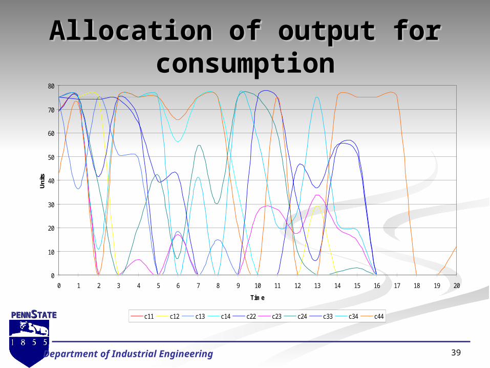
Allocation of output for Allocation of output for consumptionconsumption

0

10

20

30

40

50

60

70

80

0 1 2 3 4 5 6 7 8 9 10 11 12 13 14 15 16 17 18 19 20

Time

Uni

ts

c11 c12 c13 c14 c22 c23 c24 c33 c34 c44

40

PENNPENNSSTATETATE


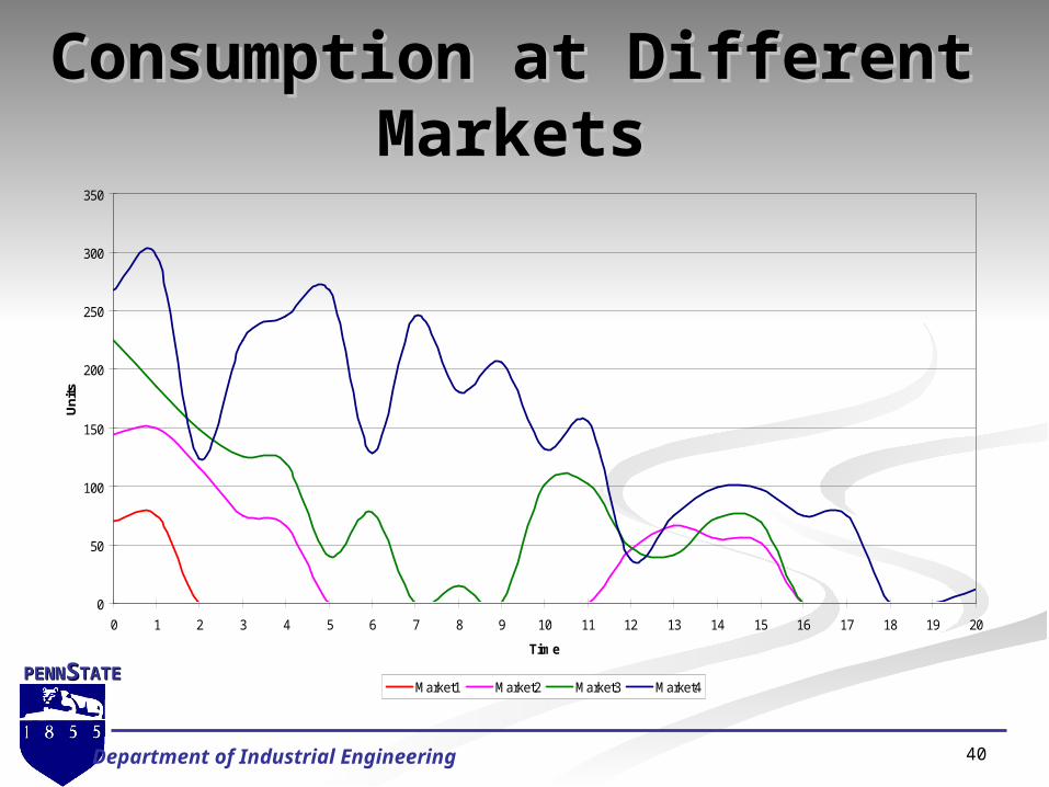
Consumption at Different Consumption at Different MarketsMarkets

0

50

100

150

200

250

300

350

0 1 2 3 4 5 6 7 8 9 10 11 12 13 14 15 16 17 18 19 20

Time

Un

its

Market1 Market2 Market3 Market4

41

PENNPENNSSTATETATE


NPV Profit of FirmsNPV Profit of Firms

0

1

2

3

4

5

6

0 1 2 3 4 5 6 7 8 9 10 11 12 13 14 15 16 17 18 19 20

Mil

lio

ns

Time

Pro

fit

($)

Firm 1 Firm 2 Firm 3 Firm 4

42

PENNPENNSSTATETATE


SummarySummary Theoretical framework and Theoretical framework and

computational experimentation of the computational experimentation of the traditional production – distribution traditional production – distribution system in a dynamic network completed system in a dynamic network completed

Theoretical framework supporting Theoretical framework supporting extensions to non-network dynamic extensions to non-network dynamic service sector environment completed. service sector environment completed.

Extensions to a dynamic network service Extensions to a dynamic network service environment in progress.environment in progress.

Numerical experiments based on Numerical experiments based on discrete time approximation of very discrete time approximation of very large problem is underwaylarge problem is underway

43

PENNPENNSSTATETATE


SummarySummary Continuous time algorithms for descent Continuous time algorithms for descent

in Hilbert space without time in Hilbert space without time discretization have been designed and discretization have been designed and analyzed qualitativelyanalyzed qualitatively

Preliminary tests of continuous time Preliminary tests of continuous time algorithms are promisingalgorithms are promising

We have shown treatment of dynamics We have shown treatment of dynamics with explicit time lags is possible using with explicit time lags is possible using continuous time algorithms. This opens continuous time algorithms. This opens the door to consideration of explicit the door to consideration of explicit service response delays – a previously service response delays – a previously unstudied topic.unstudied topic.

CONTINUED

penn s tate department of industrial engineering 1 revenue management in the context of dynamic...

Documents