penalized generalized estimating equations for high...
TRANSCRIPT

High-dimensional GEE variable selection 1
Penalized Generalized Estimating Equations for High-dimensional
Longitudinal Data Analysis
Lan Wang
School of Statistics, University of Minnesota, 224 Church Street SE, Minneapolis, MN 55455, U.S.A.
email: [email protected]
and
Jianhui Zhou
Department of Statistics, University of Virginia, Charlottesville, VA 22904, USA
email: [email protected]
and
Annie Qu
Department of Statistics, University of Illinois at Urbana-Champaign, Champaign, IL 61820 USA
email: [email protected]
Summary: We consider the penalized generalized estimating equations for analyzing longitudinal
data with high-dimensional covariates which often arise in microarray experiments and large-scale
health studies. Existing high-dimensional regression procedures often assume independent data
and rely on the likelihood function. Construction of a feasible joint likelihood function for high-
dimensional longitudinal data is challenging, particularly for correlated discrete outcome data.
The penalized generalized estimating equations procedure only requires to specify the first two
marginal moments and a working correlation structure. We establish the asymptotic theory in a
high-dimensional framework where the number of covariates pn increases as the number of clusters
n increases, and pn can reach the same order as n. One important feature of the new procedure is that
the consistency of model selection holds even if the working correlation structure is misspecified. We
evaluate the performance of the proposed method using Monte Carlo simulations and demonstrate
its application using a yeast cell-cycle gene expression data set.

Biometrics 000, 000–000 DOI: 000
000 0000
Key words: correlated data; diverging number of parameters; GEE; high-dimensional covariates;
longitudinal data; marginal regression; variable selection.
c© 0000 The Society for the Study of Evolution. All rights reserved.

High-dimensional GEE variable selection 1
1. Introduction
High-dimensional longitudinal data, which consist of repeated measurements on a large
number of covariates, have become increasingly common. In many large-scale long-term
health studies, such as the well known Framingham Heart Study, many covariates including
age, smoking status, cholesterol level, blood pressure were recorded on the participants
over the years to describe their health and lifestyles. High-dimensional data arise even
more frequently in gene expression experiments. For example, in Section 6 we analyze
a yeast cell-cycle gene expression data set where the gene expression measurements were
recorded at different time points during the cell cycle. The data set contains 297 cell-cycle
regulated genes and the covariates are the binding probabilities for 96 transcription factors.
In other examples, even though the number of variables is not large, when we include
various interaction effects the total number of covariates in the statistical model can be
considerably large. Despite the large number of covariates, it often occurs that only a subset
of them are relevant for modelling the response variable. Inclusion of redundant variables
may hinder accuracy and efficiency for both estimation and inference. Thus, it is important
to develop new statistical methodology and theory of variable selection and estimation for
high-dimensional longitudinal data.
The literature on variable selection for longitudinal data is rather limited due to the
challenges imposed by incorporating the intra-cluster correlation. Pan (2001) developed a
quasi-likelihood information criterion (QIC) which is analogous to AIC; Cantoni et al. (2005)
generalized Mallow’s Cp criterion; and Wang and Qu (2009) proposed a BIC criterion based
on the quadratic inference function. These are best subset type model selection procedures
which become computationally intensive when p is moderately large. Fan and Li (2004) and
Wang, Li and Huang (2008) studied regularized semiparametric and nonparametric marginal
models for continuous responses; Ni, Zhang and Zhang (2009) recently investigated variable

2 Biometrics, 000 0000
selection for mixed-effects model with continuous responses; Dziak (2006) and Dziak, Li
and Qu (2009) discussed the applications of SCAD-penalized quadratic inference function;
Xu et al. (2010) considered a GEE based shrinkage estimator with an artificial objective
function; Xue, Qu and Zhou (2010) proposed model selection of marginal generalized additive
model analysis for correlated data. However, the aforementioned work all assume that the
dimension of predictors is fixed. Some of these work only apply to continuous outcome
data. For correlated discrete outcome data, the joint likelihood function does not have
a close form if the correlation information is taken into account. When the dimension of
parameters diverges, numerical approximation to the joint likelihood function tends to be
computationally infeasible as it often involves high-dimensional integration.
The generalized estimating equations (GEE) approach is widely applied to longitudinal
data analysis (Liang and Zeger, 1986). An important advantage of the GEE approach is that
it yields a consistent estimator even if the working correlation structure is misspecified. In this
paper, we study the penalized GEE, which solves penalized generalized estimating equations
with a non-convex penalty function. Similarly to GEE, the penalized GEE procedure only
requires to specify the first two marginal moments and a working correlation matrix. It avoids
to specify the full joint likelihood for high-dimensional correlated data, this is particularly
appealing for modeling correlated discrete responses.
Johnson, Lin and Zeng (2008) recently derived the asymptotic theory for the penalized
estimating equations for independent data. The proposed work contains several important
new aspects: we consider multivariate correlated responses and allow the number of covariates
to diverge. To establish relevant theory with the diverging number of parameters, we employ
rather different techniques than those in Johnson, Lin and Zeng. The proposed work also
differs from the earlier penalized GEE approach with the bridge-type of penalty (Fu, 2003),
which considers the fixed “p” case and mainly aims to solve the collinearity problem.

High-dimensional GEE variable selection 3
Under the assumption of a sparse marginal model, we establish the asymptotic theory
for the penalized GEE in a high-dimensional framework where the number of candidate
covariates pn increases with the number of clusters n. The new framework allows pn to be
of size comparable to n in the sense that pn = O(n). The penalized GEE can be effectively
solved by an iterative algorithm. Furthermore, we propose a sandwich formula to estimate
the asymptotic covariance matrix.
The paper is organized as follows. In Section 2, we introduce GEE and discuss the high-
dimensional theory. In Section 3, we propose the penalized GEE and an iterative algorithm.
The theory for penalized high-dimensional GEE is presented in Section 4. In Section 5, we
report numerical results from Monte-Carlo simulations. Section 6 applies the new method to
a yeast cell-cycle gene expression data set. Sections 7 provides some discussions.
2. Generalized estimating equations
2.1 Notation and preliminaries
For the jth observation of the ith subject, we observe a response variable Yij and a pn-
dimensional vector of covariates Xij, i = 1, . . . , n and j = 1, . . . ,mi. The dimension of the
covariates pn is allowed to depend on the number of clusters n. Let Yi = (Yi1, . . . , Yimi)T
denote the vector of responses for the ith subject, and let Xi = (Xi1, . . . ,Ximi)T be the
associated mi × pn matrix of covariates. The observations are independent if they are from
different subjects, but are correlated if they are from the same subject. In what follows, we
assume mi = m <∞ for simplicity.
We denote the first two marginal moments of Yij by µij(βn) := Eβn(Yij) and σ2
ij(βn) :=
Varβn(Yij). Let µi(βn) = (µi1(βn), . . . , µim(βn))T and Ai(βn) = diag(σ2
i1(βn), . . . , σ2im(βn)).
The optimal estimating equation for βn is given by
n−1
n∑i=1
∂µi(βn)
∂βTnV−1i (Yi − µi) = 0, (1)

4 Biometrics, 000 0000
where Vi is the covariance matrix of Yi. In real applications the true intra-cluster covariance
structure is often unknown. The GEE procedure adopts a working covariance matrix which
is specified through a working correlation matrix R(τ ): Vi = A1/2i (βn)R(τ )A
1/2i (βn) where
τ is a finite dimensional parameter. Some commonly used working correlation structures
include independence, AR-1, equally correlated (also called compound symmetry) or un-
structured correlation, among others. For a given working correlation structure, τ can be
estimated using residual-based moment method.
As in Liang and Zeger (1986), we assume that the marginal density of Yij comes from a
canonical exponential family. Then we can write µij(βn) = a(θij) and σ2ij(βn) = φa(θij),
where θij = XTijβn, for a differentiable function a(·) and a scaling constant φ. With the
estimated working correlation matrix R, the estimating equations in (1) reduce to
n−1
n∑i=1
XTi A
1/2i (βn)R−1A
−1/2i (βn)(Yi − µi(βn)) = 0. (2)
We formally define the GEE estimator as the solution βn of the above estimating equations.
For eas of exposition, we assume φ = 1 in the rest of the paper. Xie and Yang (2003) and
Balan and Schiopu-Kratina (2005) established rigorous large sample theory for the GEE
when the number of clusters n is large but the dimension of covariates p is fixed.
2.2 GEE with diverging number of covariates
In a “diverging p” asymptotic framework but without the sparsity assumption, Wang (2011)
studied the consistency, asymptotic normality and validity of the sandwich variance formula
of GEE. This framework allows one to adopt a growingly more complex statistical model in
order to reduce the modeling bias.
For a vector or a matrix B, denote ||B|| = [Tr(BBT )]1/2 as its Frobenius norm, which
reduces to the Euclidean norm in the vector case. It can be shown that a preliminary GEE es-
timator βn obtained by solving the independence working estimating equation∑n
i=1XTi (Yi−

High-dimensional GEE variable selection 5
µi(βn)) = 0 satisfies ||βn−βn0|| = Op(√pn/n) when pn →∞ and p2nn
−1 = o(1), where βn0 is
the true value of βn. Under rather general conditions, using the initial consistent estimator
βn, the residual-based estimated working correlation matrix R satisfies ||R−1 − R−1|| =
Op(√pn/n), where R is a constant positive-definite matrix but not necessarily the true
correlation matrix R0.
Let
Mn(βn) =n∑i=1
XTi A
1/2i (βn)R
−1R0R
−1A
1/2i (βn)Xi,
Hn(βn) =n∑i=1
XTi A
1/2i (βn)R
−1A
1/2i (βn)Xi.
Under general regularity conditions, Wang (2011) showed that if p2nn−1 = o(1), then the
generalized estimating equation (2) has a root βn such that ||βn − βn0|| = Op(√pn/n).
Furthermore, if p3nn−1 = o(1), then ∀ αn ∈ Rpn such that ||αn|| = 1,
αTnM
−1/2
n (βn0)Hn(βn0)(βn − βn0)→ N(0, 1) in distribution.
For the purpose of variable selection for high-dimensional longitudinal data, we assume
from now on that the marginal mean regression model is sparse in the sense that most of the
covariates have zero coefficients. The above results provide some insight on how sparse the
true underlying model can be such that we are still confident about the statistical inference
after dimension reduction by variable selection. Here we allow the true underlying model size
(i.e., number of nonzero coefficients) to increase with the number of clusters but require its
dimension to be of order o(n1/3).

6 Biometrics, 000 0000
3. Penalized generalized estimating equations
3.1 Methodology
We consider the penalized generalized estimating equations for simultaneous estimation and
variable selection. Specifically, the penalized generalized estimating functions are defined as
Un(βn) = Sn(βn)− qλn(|βn|)sign(βn), (3)
where
Sn(βn) = n−1
n∑i=1
XTi A
1/2i (βn)R−1A
−1/2i (βn)(Yi − µi(βn)) (4)
are the estimating functions defining the GEE, qλn(|βn|) = (qλn(|βn1|), . . . , qλn(|βnpn|))T is a
pn-dimensional vector of penalty functions, and sign(βn) = (sign(βn1), . . . , sign(βnpn))T with
sign(t) = I(t > 0) − I(t < 0). The notation qλn(|βn|)sign(βn) denotes the component-wise
product. The tuning parameter λn determines the amount of shrinkage.
Since Un(β) has discontinuous points, an exact solution to Un(β) = 0 may not exist. We
formally define the penalized GEE estimator βn to be an approximate solution: Un(βn) =
o(an) for a sequence an → 0. The rate of an will be made clearer in Theorem 1 below.
Alternatively, we may define the penalized GEE estimator as an asymptotic zero crossing,
see Remark 2 below.
To gain insights into the penalized GEE, we first note that the penalty function qλn(|βj|)
is zero for a large value of |β|j and is relatively large for a small value of |βj|. As a result,
the generalized estimating function Snj(βn), the jth component of Sn(βn), is not penalized
if βnj is large in magnitude; while the penalty level is high if βnj is close (but not equal) to
zero and therefore forces its estimator to be shrunken to zero. Once an estimated coefficient
is shrunken to zero, it is excluded from the final selected model.
Although different penalty functions can be potentially adopted, in this paper we consider

High-dimensional GEE variable selection 7
the non-convex SCAD penalty which is given by
qλn(θ) = λn
{I(θ ≤ λn) +
(aλn − θ)+(a− 1)λn
I(θ > λn)
}for θ ≥ 0 and some a > 2. In the context of penalized likelihood, Fan and Li (2001)
demonstrated that the SCAD penalty simultaneously achieves three desirable properties
of variable selection: unbiasedness, sparsity and continuity. In contrast, the Lasso penalty
(L1 penalty) does not satisfy the unbiasedness condition, the Lq penalty with q > 1 does
not satisfy the sparsity condition, and the Lq penalty with 0 ≤ q < 1 does not satisfy the
continuity condition. Following the suggestion of Fan and Li, we take a = 3.7.
3.2 Algorithm
To solve the penalized GEE, similarly as in Johnson, Lin and Zeng (2008), we use an iterative
algorithm which combines the minorization-maximization (MM) algorithm for non-convex
penalty of Hunter and Li (2005) with the Newton-Raphson algorithm for the GEE.
For a small ε > 0, the MM algorithm suggests that the penalized GEE estimator βn =
(βn1, . . . , βnpn)T approximately satisfies
Snj(βn)− nqλn(|βnj|)sign(βnj)|βnj|
ε+ |βnj|= 0, j = 1, . . . , pn, (5)
where Snj(βn) denotes the jth element of Sn(βn). In the numerical analysis, we take ε to be
a fixed small number 10−6.
Applying the Newton-Raphson algorithm of GEE to Snj(βn) and combining with (5), we
obtain the following iterative algorithm for solving the penalized GEE:
βk
n = βk−1
n +[Hn(β
k−1
n ) + nEn(βk−1
n )]−1[
Sn(βk−1
n )− nEn(βk−1
n )βk−1
n
],

8 Biometrics, 000 0000
where
Hn(βk−1
n ) =n∑i=1
XTi A
1/2i (β
k−1
n )R−1A1/2i (β
k−1
n )Xi,
En(βk−1
n ) = diag{qλn(|βn1|+)
ε+ |βnj|, . . . ,
qλn(|βnpn|+)
ε+ |βnj|}.
Given a selected tuning parameter, we repeat the above algorithm to update βk
n for 30
iterations with the initial value β0
n = (0, 0, ..., 0)T . Our numerical experience in Section 5
indicates that the criterion∑pn
j=1 |βk+1
j − βk
j | < 0.0001 is usually met within 30 iterations.
In practice, we select the tuning parameter λn using cross-validation. More specifically, we
randomly split the data into several non-overlapping subsets of approximately equal size. We
remove one subset and fit the model to the remaining data, and estimate the prediction error
(the loss function is the negative loglikelihood under working independence assumption) from
the removed observations. This is repeated for each subset, the estimated prediction errors
are aggregated, and the best tuning parameter is selected by minimizing the aggregated
estimated prediction error over a fine grid.
Extension of the proposed penalized GEE estimator to the cases of unequal mi is straight-
forward. We vary the dimension of Ai and replace R by Ri, which is the mi × mi matrix
using the specified working correlation structure and the corresponding initial parameter τ
estimator.
4. Asymptotic theory for high-dimensional penalized GEE
In this section, we present the theory of the penalized GEE in a “large n, diverging p”
framework, which allows pn to be of similar order as n (see Remark 3 below). We denote
the true value of βn0 by βn0 = (βTn10,βTn20)
T . The covariates matrix is partitioned into
Xi = (Xi1,Xi2) accordingly. Without loss of generality, it is assumed that βn20 = 0 and
that the elements of βn10 are all nonzero. We also denote the dimension of βn10 by sn, where

High-dimensional GEE variable selection 9
sn may be fixed or grow with n. Following the discussions in Section 2·2, we assume that
sn = o(n1/3).
For the asymptotic theory, we require the following regularity conditions, which are as-
sumed for technical convenience and may be further relaxed.
(A1) Xij, 1 ≤ i ≤ n, 1 ≤ j ≤ m, are uniformly bounded.
(A2) The unknown parameter βn belongs to a compact subset B ⊆ Rpn and the true
parameter value βn0 lies in the interior of B.
(A3) There exist finite positive constants b1 and b2 such that
b1 ≤ λmin
(n−1
n∑i=1
XTi Xi
)≤ λmax
(n−1
n∑i=1
XTi Xi
)≤ b2,
where λmin (or λmax) denotes the minimum (or maximum) eigenvalue of a matrix.
(A4) The common true correlation matrix R0 has eigenvalues bounded away from zero and
+∞. The estimated working correlation matrix R satisfies ||R−1 − R−1|| = Op(
√sn/n),
where R is a constant positive-definite matrix with eigenvalues bounded away from zero and
+∞.
(A5) Let εi(βn) = (εi1(βn), . . . , εim(βn))T = A−1/2i (βn)(Yi − µi(βn)). There exists a finite
constant M1 > 0 such that E(||εi(βn0)||2+δ) ≤ M1, for all i and some δ > 0; and there
exist positive constants M2 and M3 such that E[
exp(M2|εij(βn0)|
)∣∣Xi)]≤ M3, uniformly
in i = 1, . . . , n, j = 1, . . . ,m.
(A6) Let Bn = {βn : ||βn − βn0|| ≤ ∆√pn/n}, then µ(XT
ijβn), 1 ≤ i ≤ n, 1 ≤ j ≤ m, are
uniformly bounded away from 0 and ∞ on Bn; µ(XTijβn) and µ(3)(XT
ijβn), 1 ≤ i ≤ n, 1 ≤
j ≤ m, are uniformly bounded by a finite positive constant M2 on Bn.
(A7) Assuming min1≤j≤sn |βn0j|/λn →∞ as n→∞ and s3nn−1 = o(1), λn → 0, s2n(log n)4 =
o(nλ2n), log(pn) = o(nλ2n/(log n)2), pns4n(log n)6 = o(n2λ2n) and pns
3n(log n)8 = o(n2λ4n).

10 Biometrics, 000 0000
Remark 1. The first part of condition (A5) is similar to the condition in Lemma 2 of Xie
and Yang (2003) and condition (Nδ) in Balan and Schiopu-Kratina (2005); the second part is
satisfied for Gaussian distribution, sub-Gaussian distribution and Poisson distribution, etc.
Condition (A6) requires µ(k)ij (XT
ijβn), which denotes the kth derivative of µij(t) evaluated at
XTijβn, to be uniformly bounded when βn is in a local neighborhood around βn0, k = 1, 2, 3.
This condition is generally satisfied for the GEE. For example, when the marginal model
follows a Poisson distribution, µ(t) = exp(t), thus µ(k)ij (XT
ijβn) = exp(XTijβn), k = 1, 2, 3, are
uniformly bounded around βn0 on Bn.
The regularized procedures based on minimizing the sum of an objective function and a
penalty term have been well studied for analyzing high-dimensional data, for example LASSO
(Tibshirani 1996), SCAD (Fan and Li, 2001; Fan and Peng, 2004) and MCP (Zhang, 2010),
among others. However, for the estimating equation approach, alternative techniques are
necessary to establish the asymptotic theory. Theorem 1 below characterizes the asymptotic
properties of the penalized GEE procedure.
Theorem 1: Assuming conditions (A1)-(A7), there exists an approximate penalized
GEE solution βn = (βT
n1, βT
n2)T which satisfies the following properties
(1)
P(|Unj(βn)| = 0, j = 1, . . . , sn
)→ 1 (6)
P(|Unj(βn)| ≤ λn
log n, j = sn + 1, . . . , pn
)→ 1 (7)
(2) P (βn2 = 0)→ 1;
(3) ∀ αn ∈ Rsn such that ||αn|| = 1,
αTnM
−1/2
n1 (βn0)Hn1(βn0)(βn1 − βn10)→ N(0, 1) in distribution,

High-dimensional GEE variable selection 11
where
Mn1(βn0) =n∑i=1
XTi1A
1/2i (βn0)R
−1R0R
−1A
1/2i (βn0)Xi1,
Hn1(βn0) =n∑i=1
XTi1A
1/2i (βn0)R
−1A
1/2i (βn0)Xi1.
Properties (2) and (3) in Theorem 1 are often referred to as the oracle property of variable
selection, that is, the procedure estimates the true zero-coefficient as zero with probability
approaching one and estimates the nonzero coefficients as efficiently as if the true model is
known in advance. Property (1) provides a more precise characterization for the approximate
solution of the penalized GEE.
Remark 2. Alternatively, we may define the penalized GEE estimator as an approximate
zero crossing as in Johnson, Lin and Zeng (2008). One can show that an estimator βn in
Theorem 1 is also an approximate zero crossing in the sense that a small perturbation of
βn changes the sign of the penalized estimating equations. To understand this more clearly,
we consider a perturbation of the jth component of βn, for some j = s1 + 1, . . . , pn. Such a
small perturbation leads to a penalty term of order λn which dominates the GEE part (of
order λn(log n)−1). Therefore, the direction of the perturbation determines the sign of the
penalized GEE function.
Remark 3. The number of candidate covariates pn allowed in the asymptotic theory
depends on the dimension of the true model. When the true underlying model has a fixed
dimension, which is often assumed in the literature, the above theory allows pn = o(nα) with
0 < α < 43. Note that for such pn condition (A7) is satisfied for some λn = O(n−γ), where
0 < γ < (2− α)/4, as long as min1≤j≤sn |βn0j|/λn →∞. Thus the theory allows pn to be of
similar size as n in the sense that pn = O(n).
From the algorithm in Section 3.2, we obtain the following sandwich formula to estimate
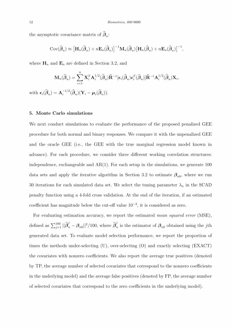
12 Biometrics, 000 0000
the asymptotic covariance matrix of βn:
Cov(βn) ≈[Hn(βn) + nEn(βn)
]−1Mn(βn)
[Hn(βn) + nEn(βn)
]−1,
where Hn and En are defined in Section 3.2, and
Mn(βn) =n∑i=1
XTi A
1/2i (βn)R−1[εi(βn)εTi (βn)]R−1A
1/2i (βn)Xi,
with εi(βn) = A−1/2i (βn)(Yi − µi(βn)).
5. Monte Carlo simulations
We next conduct simulations to evaluate the performance of the proposed penalized GEE
procedure for both normal and binary responses. We compare it with the unpenalized GEE
and the oracle GEE (i.e., the GEE with the true marginal regression model known in
advance). For each procedure, we consider three different working correlation structures:
independence, exchangeable and AR(1). For each setup in the simulations, we generate 100
data sets and apply the iterative algorithm in Section 3.2 to estimate βn0, where we run
30 iterations for each simulated data set. We select the tuning parameter λn in the SCAD
penalty function using a 4-fold cross validation. At the end of the iteration, if an estimated
coefficient has magnitude below the cut-off value 10−3, it is considered as zero.
For evaluating estimation accuracy, we report the estimated mean squared error (MSE),
defined as∑100
j=1 ||βj
n − βn0||2/100, where βj
n is the estimator of βn0 obtained using the jth
generated data set. To evaluate model selection performance, we report the proportion of
times the methods under-selecting (U), over-selecting (O) and exactly selecting (EXACT)
the covariates with nonzero coefficients. We also report the average true positives (denoted
by TP, the average number of selected covariates that correspond to the nonzero coefficients
in the underlying model) and the average false positives (denoted by FP, the average number
of selected covariates that correspond to the zero coefficients in the underlying model).

High-dimensional GEE variable selection 13
Example 1. The correlated normal responses are generated from the model
Yij = XTijβ + εij,
where i = 1, ..., 200, j = 1, ..., 4, Xij = (xij,1, ...xij,200)T is a vector of 200 covariates and
β = (2.0, 3.0, 1.5, 2.0, 0, ..., 0)T . For the covariates, we generate xij,1 from the Bernoulli(0.5)
distribution, and xij,2 to xij,200 from the multivariate normal distribution with mean 0 and
an AR(1) covariance matrix with marginal variance 1 and auto-correlation coefficient 0.5.
The random errors (εi1, ..., εi4)T are generated from the multivariate normal distribution
with marginal mean 0, marginal variance 1 and an exchangeable correlation matrix with
parameter ρ. We consider ρ = 0.5 and 0.8 to represent different strength of within cluster
correlation.
[Table 1 about here.]
The results of Table 1 summarize the estimation accuracy and model selection properties
of the penalized GEE, the unpenalized GEE and the oracle GEE for three different working
correlation matrices and two different values of ρ. We observe that in terms of estimation
accuracy the penalized GEE procedure performs closely to the oracle GEE, and significantly
reduces the MSE of the unpenalized GEE estimator. Using the true correlation structure
(exchangeable) in penalized GEE gives the smallest MSE, with greater gain when the within
cluster association is stronger. Furthermore, we observe that the unpenalized GEE generally
does not lead to a sparse model. The penalized GEE successfully selects all covariates with
nonzero coefficients and has a fairly small number of false positives. When the true working
correlation structure is used, the probability of identifying the exact underlying model (i.e.,
both false positive and false negative are zero) is about 70%.
To further investigate the performance of the penalized GEE estimator, Table 2 reports its
bias, the estimated standard deviation (calculated from the sandwich variance formula) and

14 Biometrics, 000 0000
the empirical standard deviation for estimating βi, i = 1, . . . , 4. We also use the sandwich
variance formula to construct approximate 95% confidence intervals for the four nonzero
coefficients based on the asymptotic normality theory and report the empirical coverage
probabilities. The estimated standard deviation is close to the empirical standard deviation;
and the empirical coverage probability is close to 95%. This indicated good perofrmance of
the sandwich variance formula.
[Table 2 about here.]
Example 2. The correlated binary responses have marginal mean πij satisfying
logπij
1− πij= XT
ijβ,
where i = 1, . . . , 400, j = 1, . . . , 10, Xij = (xij,1, ...xij,50)T is a vector of 50 covariates, and
β = (0.7,−0.7,−0.4, 0, 0, ..., 0)T . For the covariates, we generate xij,k independently such
that xij,k ∼ Uniform(0, 1). We use the R package “mvtBinaryEP” to generate the correlated
binary responses with an exchangeable correlation structure (ρ = 0.4) within each cluster.
We note that Example 2 is more challenging than Example 1 in two aspects: first, the
response is binary thus contains much less information than a continuous response; secondly,
we include a small signal (β3 = −0.4) in the nonzero coefficients. Table 3 summarizes
the results for estimation accuracy and model selection properties of the penalized GEE,
the unpenalized GEE and the oracle GEE for three different working correlation matrices.
We observe that the penalized GEE significantly improves the estimation accuracy of the
unpenalized GEE. The penalized GEE has high true positive rate and low false positive
rate for variable selection. We also observe that when the true correlation structure is used,
the PGEE has high probability (97%) to catch this small signal (β3 = −0.4); but when the

High-dimensional GEE variable selection 15
independence working correlation structure is used, there is a significantly higher chance to
miss this small signal.
[Table 3 about here.]
Similarly as Table 2, Table 4 reports the bias, the estimated standard deviation (calculated
from the sandwich variance formula), the empirical standard deviation, and the empirical cov-
erage probability of 95% confidence interval for estimating βi, i = 1, 2, 3, when the penalized
GEE procedure is applied. When the true correlation structure is used, the empirical coverage
probabilities for β1 and β2 are close to 95% (the estimated standard deviation is also close to
the empirical standard deviation); the empirical coverage probability for the small coefficient
β3 is close to 90% (the estimated standard deviation is smaller comparing to the empirical
standard deviation). However, when the independence working correlation structure is used,
the confidence intervals undercover the true value. These observations suggest that modeling
covariance structure is important when some of the signals are relatively weak.
[Table 4 about here.]
6. Yeast cell-cycle gene expression data analysis
We apply the penalized GEE to the yeast cell-cycle gene expression data collected in the
CDC15 experiment of Spellman et al. (1998). The experiment recorded genome-wide mRNA
levels for 6178 yeast ORFs (abbreviation for open reading frames, which are DNA sequences
that can determine which amino acids will be encoded by a gene) at 7-minute intervals for
119 minutes, which covers two cell-cycle periods for a total of 18 time points.
The cell cycle is a tightly regulated life process where cells grow, replicate their DNA,
segregate their chromosomes and divide into as many daughter cells as the environment
allows. The cell-cycle process is commonly divided into M/G1-G1-S-G2-M stages, where the
M stage stands for mitosis during which nuclear (chromosome separation) and cytoplasmic

16 Biometrics, 000 0000
(cytokinesis) and division occur, the G1 stage stands for GAP 1; the S stage stands for
synthesis during which DNA replication occurs; the G2 stage stands for GAP 2. Spellman et
al.’s experiment identified approximately 800 genes which vary in a periodic fashion during
the yeast cell cycle, however little was known about the regulation of most of these genes.
Transcription factors (TFs) have been observed to play critical roles in gene expression regu-
lation. A transcription factor (sometimes called a sequence-specific DNA-binding factor) is a
protein that binds to specific DNA sequences, thereby controlling the flow (or transcription)
of genetic information from DNA to mRNA. We next apply the penalized GEE to identify
the TFs that influence the gene expression level at each stage of the cell process. This is
important to understanding how the cell cycle is regulated and how cell cycles regulate other
biological processes.
Similarly as in Luan and Li (2003) and Wang, Li and Huang (2008), we analyze a subset
of 297 cell-cycle-regularized genes. The response variable Yij is the log-transformed gene
expression level of gene i measured at time point j; the covariates xik, k = 1, . . . , 96, is the
matching score of the binding probability of the kth transcription factor on the promoter
region of the ith gene. The binding probability is computed using a mixture modeling
approach based on data from a ChIP binding experiment, see Wang, Chen and Li (2007) for
details. We apply the penalized GEE to each of the five stages (each stage contains a few
time points from the cycle) of the cell-cycle process using the following model
Yij = α0 + α1tij +96∑k=1
βkxik + εij,
where xik, k = 1, . . . , 96, is standardized to have mean zero and variance 1; tij denotes time.
We impose penalties on the βk’s. Table 5 summarizes the number of TFs identified when
three different working correlation structures for εij are adopted: independence, AR-1 and
exchangeable.

High-dimensional GEE variable selection 17
[Table 5 about here.]
Our analysis reveals that at each of the five stages the selected TFs, in terms of both
numbers and the specific TFs, are not sensitive to the choice of the working correlation
structure. Due to the space limitation, we only report the number of selected TFs in Table
5. Some of these selected TFs have already been confirmed by biological experiments using
genome-wide binding method. For examples, Fkh1, Fkh2 and Mcm1 are three TFs that
have been proved important for stage G2 in the aforementioned biological experiments and
they have been selected by the penalized GEE for stage G2. Furthermore, the sets of TFs
selected at different stages have only small overlaps. This suggests that different TFs play
important roles at different stages of the cell-cycle process, which has also been observed by
the biologists.
7. Discussions
In general, when the number of covariates is large, identifying the exact underlying model is
a challenging task, in particular when some of the nonzero signals are relatively weak. From a
practical point of view, it is often satisfactory to identify a model that includes all important
variables along with a small number of false positives. In general, under fitting model is
more serious than over fitting in model selection. Although oracle property is suggested
by Theorem 1, the practical performance of the penalized GEE may be influenced by two
factors: (1) the multiple roots problem of the estimating equations approach and (2) the
tuning parameter selection. For the later problem, it has been observed that cross-validation
tends to select an over-fitted model. A high-dimensional BIC approach (Chen and Chen,
2008) might be more effective for selecting λn, but it is challenging to establish the relevant
theory in the GEE setting. This will be a topic of future research.

18 Biometrics, 000 0000
Acknowledgements
The authors would like to thank the two referees, the AE and the Co-Editor for their
careful reading and constructive comments which substantially improved an earlier draft.
Wang’s research is supported by National Science Foundation grant DMS-1007603; Zhou’s
research is supported by National Science Foundation grant DMS-0906665 and Qu’s research
is supported by National Science Foundation grant DMS-0906660.
Supplementary Materials
The proof of Theorem 1 is available under the Paper Information link at the the Biometrics
website http://www.tibs.org/biometrics.
References
Balan, R. M. and Schiopu-Kratina, I. (2005). Asymptotic results with generalized estimating
equations for longitudinal data. Annals of Statistic, 32, 522-541.
Cantoni, E., Flemming, J. M. and Ronchetti, E. (2005). Variable selection for marginal
longitudinal generalized linear models. Biometrics, 61, 507-514.
Chen, J. and Chen, Z. (2008). Extended Bayesian information criterion for model selection
with large model space. Biometrika, 95, 759-771.
Dziak, J. J. (2006). Penalized quadratic inference function for variable selection in longitu-
dinal research. Ph.D. Thesis, the Pennsylvania State University.
Dziak, J. J., Li, R and Qu, A. (2009) An overview on quadratic inference function approaches
for longitudinal data. In Frontiers of Statistics, Vol 1: New developments in biostatistics
and bioinformatics, edited by Fan, J., Liu, J. S. and Lin, X. World scientific publishing,
Chapter 3, 49-72.
Fan, J. and Li, R. (2001). Variable selection via nonconcave penalized likelihood and its
oracle properties. Journal of the American Statistical Association, 96, 1348-1360.

High-dimensional GEE variable selection 19
Fan, J. and Li, R. (2004). New estimation and model selection procedures for semiparametric
modeling in longitudinal data analysis. Journal of the American Statistical Association,
99, 710-723.
Fan, J. and Peng, H. (2004). Nonconcave penalized likelihood with a diverging number of
parameters. Annals of Statistics, 32, 928961.
Fu, W. J. (2003). Penalized estimating equations. Biometrics, 35, 109-148.
Hunter, D. R. and Li, R. (2005). Variable selection using MM algorithms. Annals of Statistic,
33, 1617-1642.
Johnson, B., Lin, D. Y. and Zeng, D. (2008). Penalized estimating functions and variable
selection in semiparametric regression models. Journal of the American Statistical Asso-
ciation, 103, 672-680.
Liang, K. Y. and Zeger, S. L. (1986). Longitudinal data analysis using generalized linear
models. Biometrika 73, 12-22.
Luan, Y., and Li, H. (2003). Clustering of time-course gene expression data using a mixed-
effects model with Bsplines. Bioinformatics, 19, 474482.
Pan, W. (2001). Akaike’s information criterion in generalized estimating equations. Biomet-
rics, 57, 120-125.
Spellman, P. T., Sherlock, G., Zhang, M. Q., Iyer, V. R., Anders, K., Eisen, M. B.,
Brown, P. O., Botstein, D., and Futcher, B. (1998). Comprehensive identification of cell
cycle-regulated genes of the yeast saccharomyces cerevisiae by microarray hybridization.
Molecular Biology of Cell, 9, 3273 3297.
Tibshirani, R. J. (1996). Regression shrinkage and selection via the Lasso. Journal of the
Royal Statistical Society, Series B, 58, 267–288.
Wang, L. (2011). GEE analysis of clustered binary data with diverging number of covariates.
Annals of Statistics, 39, 389-417.

20 Biometrics, 000 0000
Wang, L., Chen, G. and Li, H. (2007). Group SCAD regression analysis for microarray time
course gene expression data. Bioinformatics, 23, 1486-1494.
Wang L, Li, H. and Huang. J (2008). Variable selection in nonparametric varying- coefficient
models for analysis of repeated measurements. Journal of the American Statistical
Association, 103, 1556-1569.
Wang, L. and Qu, A. (2009). Consistent model selection and data-driven smooth tests for
longitudinal data in the estimating equations approach. Journal of the Royal Statistical
Society, Series B, 71, 177-190.
Xiao, N., Zhang, D., and Zhang H. H. (2009). Variable selection for semiparametric mixed
models in longitudinal studies. To appear in Biometrics.
Xie, M. and Yang, Y. (2003). Asymptotics for generalized estimating equations with large
cluster sizes. The Annals of Statistics, 31, 310-347.
Xu, P., Wu, P., Wang, Y. and Zhu, L.X. (2010). A GEE based shrinkage estimation for the
generalized linear model in longitudinal data analysis. Technical report, Department of
Mathematics, Hong Kong Baptist University, Hong Kong.
Xue, L, Qu, A. and Zhou, J. (2010). Efficient estimation and model selection for the marginal
generalized additive model for correlated data. To appear in Journal of the American
Statistical Association.
Zhang, C. H. (2010). Nearly unbiased variable selection under minimax concave penalty.
Annals of Statistics, 38, 894-942.

High-dimensional GEE variable selection 21
Table 1: Correlated continuous responses (n = 200, pn = 200): comparison of GEE, oracleGEE and penalized GEE with three different working correlation matrices (independence,exchangeable and ar1).
MSE U O EXACT TP FP
ρ = 0.5GEE.indep 0.568 0.00 1.00 0.00 4.00 193.02GEE.exch 0.381 0.00 1.00 0.00 4.00 192.45GEE.ar1 0.458 0.00 1.00 0.00 4.00 192.66Oracle.indep 0.009 - - - - -Oracle.exch 0.006 - - - - -Oracle.ar1 0.007 - - - - -PGEE.indep 0.009 0.00 0.85 0.15 4.00 2.02PGEE.exch 0.008 0.00 0.33 0.67 4.00 3.30PGEE.ar1 0.008 0.00 0.38 0.62 4.00 3.00
ρ = 0.8GEE.indep 0.568 0.00 1.00 0.00 4.00 193.01GEE.exch 0.165 0.00 1.00 0.00 4.00 190.44GEE.ar1 0.211 0.00 1.00 0.00 4.00 191.53Oracle.indep 0.010 - - - - -Oracle.exch 0.003 - - - - -Oracle.ar1 0.003 - - - - -PGEE.indep 0.011 0.00 0.83 0.17 4.00 2.15PGEE.exch 0.004 0.00 0.33 0.67 4.00 4.23PGEE.ar1 0.005 0.00 0.35 0.65 4.00 4.02
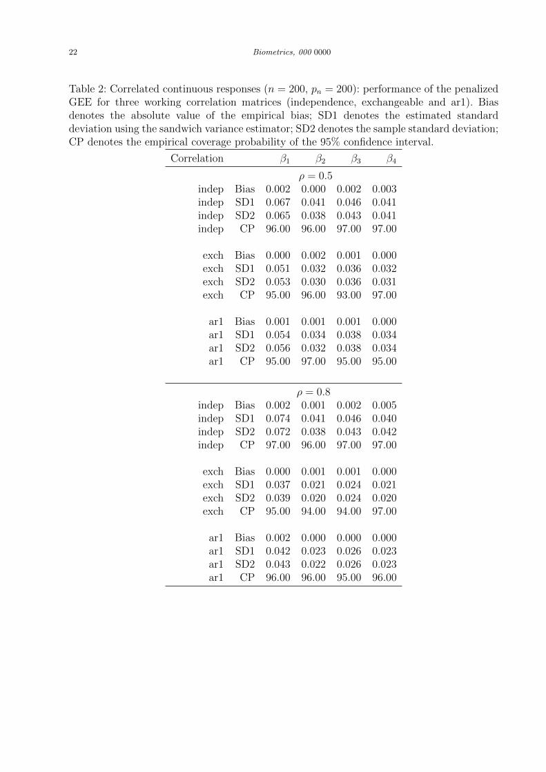
22 Biometrics, 000 0000
Table 2: Correlated continuous responses (n = 200, pn = 200): performance of the penalizedGEE for three working correlation matrices (independence, exchangeable and ar1). Biasdenotes the absolute value of the empirical bias; SD1 denotes the estimated standarddeviation using the sandwich variance estimator; SD2 denotes the sample standard deviation;CP denotes the empirical coverage probability of the 95% confidence interval.
Correlation β1 β2 β3 β4
ρ = 0.5indep Bias 0.002 0.000 0.002 0.003indep SD1 0.067 0.041 0.046 0.041indep SD2 0.065 0.038 0.043 0.041indep CP 96.00 96.00 97.00 97.00
exch Bias 0.000 0.002 0.001 0.000exch SD1 0.051 0.032 0.036 0.032exch SD2 0.053 0.030 0.036 0.031exch CP 95.00 96.00 93.00 97.00
ar1 Bias 0.001 0.001 0.001 0.000ar1 SD1 0.054 0.034 0.038 0.034ar1 SD2 0.056 0.032 0.038 0.034ar1 CP 95.00 97.00 95.00 95.00
ρ = 0.8indep Bias 0.002 0.001 0.002 0.005indep SD1 0.074 0.041 0.046 0.040indep SD2 0.072 0.038 0.043 0.042indep CP 97.00 96.00 97.00 97.00
exch Bias 0.000 0.001 0.001 0.000exch SD1 0.037 0.021 0.024 0.021exch SD2 0.039 0.020 0.024 0.020exch CP 95.00 94.00 94.00 97.00
ar1 Bias 0.002 0.000 0.000 0.000ar1 SD1 0.042 0.023 0.026 0.023ar1 SD2 0.043 0.022 0.026 0.023ar1 CP 96.00 96.00 95.00 96.00

High-dimensional GEE variable selection 23
Table 3: Correlated binary responses (n = 400, pn = 50): comparison of GEE, oracleGEE and penalized GEE with three different working correlation matrices (independence,exchangeable and ar1).
MSE U O EXACT TP FP
GEE.indep 0.635 0.00 1.00 0.00 3.00 46.51GEE.exch 0.421 0.00 1.00 0.00 3.00 46.60GEE.ar1 0.576 0.00 1.00 0.00 3.00 46.59Oracle.indep 0.027 - - - - -Oracle.exch 0.018 - - - - -Oracle.ar1 0.025 - - - - -PGEE.indep 0.111 0.28 0.32 0.40 2.72 0.93PGEE.exch 0.049 0.03 0.37 0.60 2.97 1.05PGEE.ar1 0.081 0.09 0.37 0.54 2.91 1.33

24 Biometrics, 000 0000
Table 4: Correlated binary responses (n = 400, pn = 50): performance of the penalized GEEfor three working correlation matrices (independence, exchangeable and ar1). Bias denotesthe absolute value of the empirical bias; SD1 denotes the estimated standard deviation usingthe sandwich variance estimator; SD2 denotes the sample standard deviation; CP denotesthe empirical coverage probability of the 95% confidence interval.
Correlation β1 β2 β3
indep Bias 0.038 0.048 0.107indep SD1 0.099 0.101 0.066indep SD2 0.119 0.125 0.221indep CP 85.00 87.00 64.00
exch Bias 0.001 0.005 0.027exch SD1 0.081 0.083 0.076exch SD2 0.078 0.082 0.128exch CP 94.00 95.00 88.00
ar1 Bias 0.010 0.017 0.050ar1 SD1 0.089 0.090 0.077ar1 SD2 0.087 0.095 0.171ar1 CP 96.00 98.00 81.00

High-dimensional GEE variable selection 25
Table 5: Number of TFs selected for each stage in the yeast cell-cycle process with thepenalized GEE procedure
Correlation M/G1 G1 S G2 M
indep 20 19 19 10 22exch 20 18 18 10 18ar1 23 17 18 10 19