pedestrian detection image processing with fpga - … pedestrian detection image processing with...
TRANSCRIPT

i
Pedestrian Detection Image Processing with FPGA
A Major Qualifying Project Report
Submitted to the faculty of the
WORCESTER POLYTECHNIC INSTITUTE
in partial fulfillment of the requirements of the
Degree of Bachelor of Science
By:
Jiye Duan, Electrical and Computer Engineering
William MacDowell, Electrical and Computer Engineering
Submitted to: Project Advisor: Professor Xinming Huang, Department of Electrical and
Computer Engineering
Submitted on April 30, 2014

ii
Abstract
This paper focuses on real-time pedestrian detection using the Histograms of Oriented Gradients
(HOG) feature descriptor algorithm in combination with a Linear Support Vector Machine
(LSVM) on a Field Programmable Gate Array (FPGA). Pedestrian detection on embedded
systems is a challenging problem since accurate recognition requires extensive computation. To
achieve real-time pedestrian recognition on embedded systems, hardware architecture suitable
for HOG feature extraction is proposed. HOG is considered the most accurate pedestrian
detection algorithm in modern computer vision. In order to reduce computational complexity
toward efficient hardware architecture, this paper proposes several methods to simplify the
computation of the HOG feature descriptor such as conversion of the division, square root, and
arctangent to more simple operations. The architecture is proposed on a Xilinx Zynq-7000 All
Programmable SoC ZC702 using Verilog HDL to evaluate the real-time performance. This
implementation processes image data at twice the pixel rate of similar software simulations and
significantly reduces resource utilization while maintaining high detection accuracy.
iii
Acknowledgements
Our group would like to acknowledge everyone that helped to provide an opportunity to
take part in this project and the great success that resulted from it.
First and foremost, we would like to express our greatest appreciation to our advisor, Dr.
Xinming Huang for his generous guidance, advice and motivation throughout this study. His
critical suggestion and comments help us to develop the study project into understandable and
workable effort.
Furthermore, we would like to thank the graduate students in the Embedded Computing
Lab at WPI for their support. Particularly Boyang Li and Yuteng Zhou without whom this
project would not have been possible.
We would like to sincerely thank the Worcester Polytechnic Institute (WPI) for providing
the facilities and equipment for this research
Without the assistance of these individuals, this project would not have been the success
that it was. Thank you!

iv
Authorship
This report was developed through a collaborative effort by both members of the project
team: William MacDowell and Jiye Duan. All sections were created and edited as a team, with
equal contributions made by each member.

v
Table of Contents Abstract ......................................................................................................................................................... ii
Acknowledgements ...................................................................................................................................... iii
Authorship ................................................................................................................................................... iv
Table of Figures ........................................................................................................................................... vii
Executive Summary .................................................................................................................................... viii
Chapter 1: Introduction ................................................................................................................................ 1
1.1 Pedestrian Detection .......................................................................................................................... 1
1.2 Histogram of Oriented Gradients (HOG)............................................................................................. 2
1.3 Support Vector Machine (SVM) .......................................................................................................... 8
Chapter 2: Software Simulation .................................................................................................................. 12
2.1 OpenCV ............................................................................................................................................. 12
2.2 Matlab ............................................................................................................................................... 17
2.3 Summary ........................................................................................................................................... 22
Chapter 3: Hardware Design ....................................................................................................................... 23
3.1 Introduction to Xilinx Zynq-7000 FPGA ............................................................................................. 23
3.1.1 Zynq-7000 EPP ZC702 Evaluation Kit ......................................................................................... 24
3.1.2 HDMI I/O FMC Module .............................................................................................................. 26
3.2 Design Specifications ........................................................................................................................ 28
3.2.1 HDMI I/O FMC Pass-Through Demo .......................................................................................... 29
3.2.2 Proposed Overall Hardware Architecture Design ...................................................................... 30
3.3 FPGA Design Components ................................................................................................................ 30
3.3.1 Scaling ........................................................................................................................................ 30
3.3.2 Gradient Computation ............................................................................................................... 31
3.3.3 Gradient Orientation Binning ..................................................................................................... 33
3.3.4 Histogram Generation................................................................................................................ 34
3.3.5 Normalization................................................................................................................................. 35
3.4 Evaluation ......................................................................................................................................... 36
3.5 Summary ........................................................................................................................................... 36
Chapter 4: Conclusions and Future Work ................................................................................................... 37
References .................................................................................................................................................. 38
Appendix A: peopledetect.cpp ................................................................................................................... 40
Appendix B: videostream.cpp ..................................................................................................................... 44
vi
Appendix C: videopeopledetect.cpp ........................................................................................................... 45
Appendix D: 1framepeopledetect.cpp ........................................................................................................ 46
Appendix E: HOG Top Module .................................................................................................................... 48
Appendix F: Gradient Calculating Top Module ........................................................................................... 49
Appendix G: Gradient First Derivative Calculating Module ........................................................................ 50
Appendix H: Luminous Input Module ......................................................................................................... 51
Appendix I: Gradient Direction Calculating Module ................................................................................... 52
Appendix J: Gradient Magnitude Calculating Module (LUT) ...................................................................... 54
Appendix K: Histogram Top Module ........................................................................................................... 55
Appendix L: Histogram Block Module ......................................................................................................... 56
Appendix M: Normalization Block Module ................................................................................................. 57
Appendix N: SRAM Controller Module ....................................................................................................... 58
Appendix O: Histogram Storing Module ..................................................................................................... 60

vii
Table of Figures
Figure 1: An overview of our feature extraction and object detection chain. The detector window is tiled
with a grid of overlapping blocks in which Histogram of Oriented Gradient feature vectors are extracted.
The combined vectors are fed to a linear SVM for classification [3]. ........................................................... 3
Figure 2: Dividing the image window into cells. ........................................................................................... 4
Figure 3: Orientation Binning. Each cell contains 64 pixels and are binned into 9 bins according to their
orientation [4]. .............................................................................................................................................. 4
Figure 4: Class determination at the histogram creation step [12]. ............................................................. 6
Figure 5: Block normalization. Each block contains 4 cells and are normalized respective to the block [4].
...................................................................................................................................................................... 7
Figure 6: Histogram of Oriented Gradient [4]. .............................................................................................. 8
Figure 7: Visual representation of the definitions associated with SVM [13]. ............................................. 9
Figure 8: Example of the OpenCV HOG algorithm using the built-in webcam ........................................... 13
Figure 9: Alternative example of OpenCV's HOG algorithm in conjunction with the webcam .................. 14
Figure 10: Detected pedestrians in an INRIA image with the OpenCV HOG algorithm .............................. 15
Figure 11: Missed pedestrian in an INRIA image with the OpenCV HOG algorithm .................................. 16
Figure 12: False positive in an INRIA image with the OpenCV HOG algorithm .......................................... 16
Figure 13: HOG visualization object vs. original image ............................................................................... 19
Figure 14: 1GB DDR3 DRAM on Xilinx Zynq-7000 ...................................................................................... 25
Figure 15: Dual Cortex-A9 CPU in Zynq-7000 processing system [4] ......................................................... 26
Figure 16: HDMI I/O FMC module block diagram [16] ............................................................................... 27
Figure 17: Real HDMI I/O FMC module ....................................................................................................... 28
Figure 18: HDMI Pass-Through Block Diagram [16] .................................................................................... 29
Figure 19: Proposed overall hardware Architecture................................................................................... 30
Figure 20: Proposed hardware architecture of gradient computation ...................................................... 32
Figure 21: Angular quantization into 9 evenly spaced orientation bins over 0 – 180 degree (signed
gradient) ...................................................................................................................................................... 33
Figure 22: Proposed architecture of Gx(x, y)*tan20° .................................................................................. 33
Figure 23: Proposed processing element in the sliding window detector ................................................. 34
Figure 24: Proposed hardware architecture of the entire HOG algorithm [12] ......................................... 35

viii
Executive Summary
Due to the rise in automobile use over the last century, and its continued rise today, road
accidents have become a prominent cause of injury and death. The knowledge in the field of
computer vision continues to grow, so too does the realization of its potential benefits in the area
of driver safety. Over the past few years, many recognition algorithms have been proposed to
assist in the area of driver safety, but very few of them are both accurate and fast enough for real-
time processing. This major qualifying project aims to further develop one of these algorithms
for high accuracy and real-time performance in the area of pedestrian detection from an
automobile.
Detecting pedestrians in an image has proven to be a challenging task for many
researchers due to the wide variability in possibilities. Posture, clothing, size, background, and
weather all can be impactful on the appearance of an image. This was the motivation behind a
robust feature extraction algorithm, namely Histograms of Oriented Gradients (HOG). The
algorithm divides each image into a grid. Each cell of the grid is represented by a histogram
which contains information on the orientation of the gradients within the cell. A concatenation of
these histograms produces a final feature vector which can be used for classification with a linear
Support Vector Machine (SVM) or other statistical classification tool. Compared to other feature
extraction algorithms used for pedestrian detection, HOG has far better results in terms of
accuracy. The accuracy stems from the overlapping of cells in the grid which makes the final
feature vector more robust to local contrast in the image. This project is intended to use a
hardware approach to HOG such that the same accuracy may be achieved in real-time.
Software simulation laid the framework for development of the hardware architecture for
HOG. OpenCV, an open source computer vision library, has a HOG function which was the

ix
starting point for our software simulation. The function, written in C++, is a solid proof of
concept that HOG does in fact work; however, when implemented with a webcam it becomes
apparent that real-time constraints are not met. As a basis for the hardware implementation, a
Matlab function was developed. The function was checked against the Matlab Computer Vision
Toolbox’s extractHOGFeatures and once similarity was confirmed, it was tested with the SVM
classifier. 251 out of 288 pedestrians were positively classified while all of the non-pedestrians
were correctly classified.
Hardware implementation is targeted on the Xilinx-7000 ZC702 evaluation kit. We
divided the entire HOG algorithm into several modules and designed them by using Verilog
HDL in Xilinx ISE design tools. A demo that has been successfully tested was to accept the
image input from one laptop through HDMI IN on HDMI I/O FMC and output the image on
another monitor through HDMI OUT. Our main idea was to modify the hardware architecture of
the demo and add our own HOG hardware module into it that is processing video frames
continuously. We suggest that in the future this hardware architecture be integrated into an all-
encompassing automobile computer vision device. Such a device would have various algorithms
for all aspects of computer vision for driver assistance. This project is just one piece of the bigger
picture.

1
Chapter 1: Introduction
1.1 Pedestrian Detection
Pedestrian recognition is one of the most challenging problems in the field of computer
vision. There have been many recognition algorithms proposed for purposes such as prevention
of traffic accidents by using vehicle cameras. For embedded systems, however, a recognition
algorithm that achieves not only high accuracy but also real-time processing in an environment
with limited resources is required. Pedestrian detection is also an essential and significant task in
any intelligent video surveillance system, as it provides the fundamental information
for semantic understanding of the video footages.
Due to the rise in the popularity of automobiles over the last century, road accidents have
become a major cause of fatalities. About 10 million people become traffic casualties around the
world each year, and two to three million of these people are seriously injured [1,2]. For
instance, in 2003, the United Nations reported almost 150,000 injured and 7,000 killed in
vehicle-to-pedestrian accidents just in the European Union alone.
The major challenge of pedestrian protections systems (PPSs) is the development of
reliable on-board pedestrian detection systems. Due to the varying appearance of pedestrians
e.g., different clothes, changing size, aspect ratio, and dynamic shape and the unstructured
environment, it is very difficult to cope with the demanded robustness of this kind of system.
Two problems arising in this research area are the lack of public benchmarks and the difficulty in
reproducing many of the proposed methods, which makes it difficult to compare the approaches.
As a result, surveying the literature by enumerating the proposals one-after-another is not the

2
most useful way to provide a comparative point of view. These challenges are summarized by
the following points:
The appearance of pedestrians exhibits very high variability since they can change pose,
wear different clothes, carry different objects, and have a considerable range of sizes
especially in terms of height.
Pedestrians must be identified in outdoor urban scenarios, i.e., they must be detected in
the context of a cluttered background, urban areas are more complex than highways
under a wide range of illumination, and weather conditions that vary the quality of the
sensed information e.g., shadows and poor contrast in the visible spectrum. In addition,
pedestrians can be partially occluded by common urban elements, such as parked
vehicles or street furniture.
Pedestrians must be identified in highly dynamic scenes since both the pedestrian and
camera are in motion, which complicates tracking and movement analysis. Furthermore,
pedestrians appear at different viewing angles.
The required performance is quite demanding in terms of system reaction time and
robustness i.e., false alarms versus misdetections.
1.2 Histogram of Oriented Gradients (HOG)
Detecting pedestrian in images is a challenging task owing to their variable appearance
and the wide range of poses that they can adopt. The first need is a robust feature set that allows
the pedestrian form to be discriminated cleanly, even in cluttered backgrounds under difficult
illumination. We study the issue of feature sets for pedestrian detection, showing that locally
normalized Histogram of Oriented Gradient (HOG) descriptors provide excellent performance
3
relative to other existing feature sets including wavelets. For simplicity and fast processing time,
we use linear SVM as a baseline classifier throughout the study.
HOG are feature descriptors used in computer vision and image processing for the
purpose of object detection. The technique counts occurrences of gradient orientation in
localized portions of an image. This method is similar to that of edge orientation
histograms, scale-invariant feature transform descriptors, and shape contexts, but differs in that it
is computed on a dense grid of uniformly spaced cells and uses overlapping local contrast
normalization for improved accuracy.
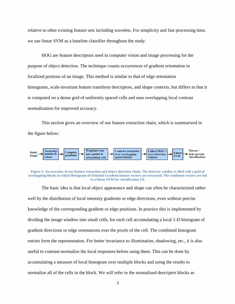
This section gives an overview of our feature extraction chain, which is summarized in
the figure below:
Figure 1: An overview of our feature extraction and object detection chain. The detector window is tiled with a grid of
overlapping blocks in which Histogram of Oriented Gradient feature vectors are extracted. The combined vectors are fed
to a linear SVM for classification [3].
The basic idea is that local object appearance and shape can often be characterized rather
well by the distribution of local intensity gradients or edge directions, even without precise
knowledge of the corresponding gradient or edge positions. In practice this is implemented by
dividing the image window into small cells, for each cell accumulating a local 1-D histogram of
gradient directions or edge orientations over the pixels of the cell. The combined histogram
entries form the representation. For better invariance to illumination, shadowing, etc., it is also
useful to contrast-normalize the local responses before using them. This can be done by
accumulating a measure of local histogram over multiple blocks and using the results to
normalize all of the cells in the block. We will refer to the normalized descriptor blocks as

4
Histogram of Oriented Gradient (HOG) descriptors. Tiling the detection window with a dense,
overlapping grid of HOG descriptors and using the combined feature vector in a conventional
SVM based window classifier gives our human detection chain as shown in Figure 1.
1. Image Window: It uses a spatial widowing method of 64 × 128 pixels. This is done to
obtain the initial object location. The detection window will be shifted and scaled
throughout the image and the HOG feature is extracted for each window.
Figure 2: Dividing the image window into cells.
Figure 3: Orientation Binning. Each cell contains 64 pixels and are binned into 9 bins according to their orientation [4].

5
2. Gradient Computation: Point derivatives Gx and Gy are computed by convolving
gradient mask and with the raw image. Refer equation (1.1) and (1.2).
Gx = Mx * I Mx = [ -1 0 1 ] (1.1)
Gy = My * I My = [ -1 0 1 ]T (1.2)
Where I, is the image.
3. Then the gradient magnitude (|G(x, y)|) and orientation angle (θ) are obtained. Refer
equation (1.3) and (1.4):
| ( )| √ ( ) ( ) (1.3)
( ) ( )
( ) (1.4)
4. Orientation Binning: The orientation bins are evenly spaced over 0° - 180° for
“unsigned” gradient or 0° - 360° for “signed” gradient. The window is then split into
a dense grid where each block is called a cell. Each pixel within a cell are placed
within the bin based on orientation. A histogram is then created for each cell. The
best performance obtained for human detection is by having 2 × 2 pixels per cell [12].
For the arctangent operation, more specific simplification is applied. The arctangent
operation is required for computation of θ(x, y) that is used only to determine class
of a histogram. Hence, we can simplify the arctangent operation to comparing
operations that satisfy the following condition (1.5):
( ) ( ) ( ) (1.5)
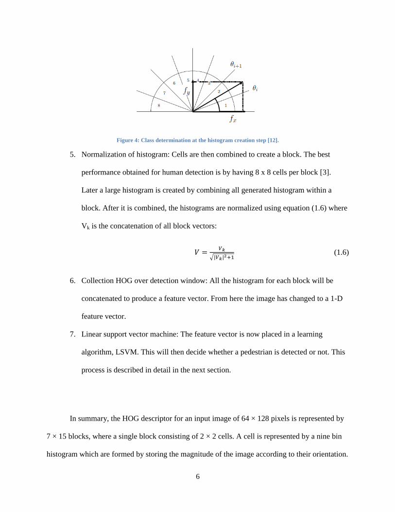
6
Figure 4: Class determination at the histogram creation step [12].
5. Normalization of histogram: Cells are then combined to create a block. The best
performance obtained for human detection is by having 8 x 8 cells per block [3].
Later a large histogram is created by combining all generated histogram within a
block. After it is combined, the histograms are normalized using equation (1.6) where
Vk is the concatenation of all block vectors:
√| | (1.6)
6. Collection HOG over detection window: All the histogram for each block will be
concatenated to produce a feature vector. From here the image has changed to a 1-D
feature vector.
7. Linear support vector machine: The feature vector is now placed in a learning
algorithm, LSVM. This will then decide whether a pedestrian is detected or not. This
process is described in detail in the next section.
In summary, the HOG descriptor for an input image of 64 × 128 pixels is represented by
7 × 15 blocks, where a single block consisting of 2 × 2 cells. A cell is represented by a nine bin
histogram which are formed by storing the magnitude of the image according to their orientation.

7
This gives us a total of (7 × 15) × (2 × 2) × 9 = 3780 features. A 2-dimensional data (64 × 128) is
converted to a 1-dimensional full feature vector (1 × 3780).
Figure 5: Block normalization. Each block contains 4 cells and are normalized respective to the block [4].

8
Figure 6: Histogram of Oriented Gradient [4].
1.3 Support Vector Machine (SVM)
Support vector machines are supervised learning models used in modern day machine
learning algorithms to detect patterns in data in pursuance of the overall goal of classification.
SVM has become one of the fastest methods of modern machine learning and is currently on the
forefront of the field for its speed and simplicity. The learning algorithm is given a set of training
data each classified in one of two categories. The algorithm builds a model for new data to be
placed based on the characteristics of the training data set. It is for this reason that SVM is
considered to be a binary linear classifier.
Training data is placed in N-dimensional space and a hyperplane separates the two
categories. In general there can be an infinite number of hyperplanes separating the two classes.
The “best” hyperplane, however, is one with the largest margin between the two different
categories of data. A support vector is the vector connecting two data points in one category that
is closest to the hyperplane. Margin is defined as the maximum distance between the support

9
vectors of the two categories assuming there are no data points within it. This is all portrayed
graphically in Figure 7 where + represents one class of data and – represents the other.
Figure 7: Visual representation of the definitions associated with SVM [13].
It is clear from the figure above that the larger the margin in the model, the more
certainty there is in making classification decisions. This is considered a classification safety
margin: a slight error in measurement will not cause misclassification. More formally, the
decision hyperplane can be defined by an intercept term and a hyperplane normal vector .
This vector is commonly known in the machine language field as the weight vector. The
hyperplane is perpendicular to the normal vector, and as a result all points on the hyperplane
satisfy equation (1.7).
(1.7)
Assume the training data set is represented by {( )} where each member, i, is a pair of
points and class labels y. The class labels take the form of +1 or -1 for simplicity and the
10
intercept term is always explicitly stated as b instead of being grouped in with the weight vector.
Thus, the linear classifier, resulting in either +1 or -1, is represented by equation (1.8).
( ) ( ) (1.8)
The functional margin of the ith
data with respect to the hyperplane is represented as
( ). Furthermore, the functional margin of an entire dataset is twice the functional
margin of the point with the smallest functional margin. This geometry is previously displayed
in Figure 7. The fundamental flaw with this approach is that the functional margin is
underconstrained. The functional margin can always be increased by simply scaling the weight
vector and the intercept term. Since a large functional margin is always the goal, but it can be so
easily scaled, more constraints on the size of the weight vector must be applied.
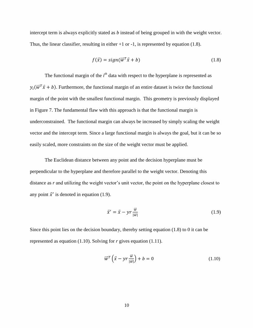
The Euclidean distance between any point and the decision hyperplane must be
perpendicular to the hyperplane and therefore parallel to the weight vector. Denoting this
distance as r and utilizing the weight vector’s unit vector, the point on the hyperplane closest to
any point is denoted in equation (1.9).
| | (1.9)
Since this point lies on the decision boundary, thereby setting equation (1.8) to 0 it can be
represented as equation (1.10). Solving for r gives equation (1.11).
(
| |) (1.10)

11
| | (1.11)
The geometric margin is considered the maximum length of a line that can be drawn
between the two support vectors as seen in Figure 7. It may also be represented as two times the
minimum r from equation (1.11). Now it becomes clear that the margin, geometrically, is
invariant to scaling of the hyperplane parameters because it is normalized using the length of the
weight vector. Since the functional margin can be scaled, for large SVMs it is standard to require
that it be greater than one for all data vectors and that it is equal to one for at least one data
vector as shown in equation (1.12).
( ) (1.12)
Using equation (1.11) above, it is clear that the geometric margin can be represented as
| |
and it is still our goal to maximize the geometric margin in an attempt to make the most robust
model possible. This can be considered the same as minimizing the inverse of the geometric
mean which leaves the formulation of a SVM as a minimization problem:
{( )}
( )
Quadratic optimization problems are a well-known class of mathematical optimization
problems and there are a wide variety of ways to solve them [11]. The details of such solutions are
usually abstract to the user of any modern SVM packages, like SVMlite [14], and are outside of the
scope of the work done for this major qualifying project.

12
Chapter 2: Software Simulation
The final goal of this Major Qualifying Project is to design the HOG algorithm for use on
an FPGA as an embedded platform for driver assistance functions. To achieve this goal, we first
attempt to realize the algorithm in software then convert our algorithm to Verilog code and
implement on an FPGA. As such, this chapter has three main purposes:
1. To delineate the variety of software implementations for the HOG algorithm.
2. To understand how different implementations can provide different descriptors as
outputs but still be successful in classification with SVM.
3. To realize the necessity for hardware implementation to achieve real-time results.
2.1 OpenCV
OpenCV is an open source library for computer vision and machine learning [15]. The
library, written in C++, has various interfaces including C++, C, Python, Java, and MATLAB.
There are currently over 500 algorithms that compose the library. Here we use the C++ library
and some built in functionality surrounding HOG and SVM. Our implementation of the
following methodology was performed on a Windows 8 PC using eclipse for writing code and
MinGW for compiling. OpenCV is used to check the functionality of HOG as a pedestrian
detector from a higher level. This means that the details of the algorithm are abstract here
because HOG is one of the built-in functions provided by OpenCV. This function provided a
strong starting point for software simulation in that it showed us the capabilities i.e. detecting
pedestrians and limitations i.e. speed and accuracy, of HOG in software.
One program that is provided in the OpenCV master sample list is peopledetect.cpp
(Appendix A). This program detects pedestrians in an image or a series of images using the class
HOG Descriptor which contains all of the functions associated with the HOG algorithm. The

13
OpenCV reference manual also provides a short piece of code to stream input from a webcam
onto the computer monitor (Appendix B). A simple combination of these two functions, video
streaming with people detection and it is evident that the HOG algorithm is successfully
detecting people from a webcam.
Figure 8: Example of the OpenCV HOG algorithm using the built-in webcam
The code begins by setting a standard capture size for the webcam, 320 x 240. This can
be adjusted if necessary and the function will still succeed. Then, the SVM is set using
OpenCV’s default SVM for people detection. In an infinite loop, the detectMultiScale function
from the HOGDescriptor class is called. This function takes the input image and outputs a
rectangular vector containing the locations for positive pedestrian matches. Here, we choose to
increase the window size by 1.05 in every iteration so as to detect different sizes of people in an
image. The remainder of the code is fairly straightforward. It uses the found locations to draw a
rectangle around detected people and output that onto the computer monitor using the imshow
function. The full code is shown in Appendix C.

14
It should be noted that this implementation is fairly slow and definitely not suitable for
real-time pedestrian detection from an automobile. This is due to both of the two following
factors. The propagation delay from the low-quality, built-in webcam is high enough to cause
delay in real-time detection. This is more evident when the video output size on the PC monitor
is increased because the video output is delayed when the input is in motion. Even at a 50
percent increase in the x and y directions, it is clear that the on-screen output takes over a second
to propagate. The other reason is in the miss-rate of the OpenCV HOG implementation. This
miss rate will be described later in this section with still-frame photos; however, the necessity for
hardware implementation is already becoming clear.
Figure 9: Alternative example of OpenCV's HOG algorithm in conjunction with the webcam
Nearly identical code was used for testing on still-frame images; however, the webcam
code is exchanged for code that takes a list of image file names as an argument and returns each
image with the algorithm run on it one by one (Appendix D). It is with this implementation that
the true shortcomings of the OpenCV HOG algorithm are discovered. The INRIA pedestrian
dataset is used to test the efficiency of the algorithm. This dataset is the original one used for

15
HOG, by Dalal and Triggs, and continues today to be the standard across the field of pedestrian
detection [9]. With this still-frame testing it becomes clear that within different images all three
possible scenarios exist: detected pedestrian, missed pedestrian, and false positive. Examples of
each follow in Figure 10, Figure 11, and Figure 12.
Figure 10: Detected pedestrians in an INRIA image with the OpenCV HOG algorithm

16
Figure 11: Missed pedestrian in an INRIA image with the OpenCV HOG algorithm
Figure 12: False positive in an INRIA image with the OpenCV HOG algorithm

17
All of the above findings show that the OpenCV HOG algorithm is a success, but it has
limitations. It serves as a strong foundation for understanding the basics of HOG and how to
implement it with C++. The limitations including speed, miss rate, and false positives are the
motivation for investigating hardware implementation as an alternative. Prior to doing that, a less
abstract version of the algorithm must be developed such that the hardware code can perform the
same functions as in software. As part of this major qualifying project the aforementioned is
implemented in Matlab.
2.2 Matlab
Since the OpenCV HOG implementation is fairly abstract, Matlab is the main source of
software testing used. Matlab, like OpenCV, has a built-in HOG algorithm. Another similarity
between MATLAB and OpenCV as it relates to their HOG implementations is that the built-in
functions are indeed viewable by the user. The downfall is that these functions are hundreds of
lines of code and it is difficult to make modifications to them. This is the motivation for writing a
separate piece of Matlab code to output an HOG descriptor and subsequently compare that
output with the output of the built-in function. If the output is indeed usable, then the Matlab
code could serve as the basis for writing fixed point Verilog code.
The Matlab Computer Vision System Toolbox provides algorithms, functions, and
applications for the design and testing of computer vision systems. The toolbox has various
capabilities including, but not limited to, object detection, feature extraction, feature matching
and stereo vision. The toolbox also provides a set of video processing functions including video
display, object annotation, and drawing graphics.
One algorithm found in the Computer Vision System Toolbox, available in Matlab
R2013b and later, is extractHOGFeatures. This function takes either a truecolor or grayscale

18
image as input and returns a 1-by-N feature vector as output using HOG. While the code is
available to edit, it is lengthy and complex to alter. For the purposes of this project, it is best to
understand the key functions and attempt to replicate it rather than try to alter the details of it.
There are certain values that are available for editing upon calling the function from the
command line. These values help to better understand the details of the function. A list of these
name-value pair arguments is as follows:
‘CellSize’ – size of the HOG cell specified in pixels as a 2-element vector.
Increasing the cell size allows for larger spatial capture of information but risks
losing small detail. Default value: [8 8]
‘BlockSize’ – number of cells in a block expressed as a 2-element vector. Larger
blocks risk losing the ability to distinguish local illumination changes. There are
more pixels in a large block and their local changes could be lost with averaging.
It is best to keep blocks small. Default value: [2 2]
‘BlockOverlap’ – number of overlapping cells between adjacent blocks as a 2-
element vector. Large overlap values can capture more information but they result
in larger feature vectors. It is recommended to overlap at least half of each block.
Default value: ceil(BlockSize/2)
‘NumBins’ – number of histogram orientation bins represented as a scalar. Finer
orientation details require more bins at the cost of larger feature vectors. Default
value: 9
‘UseSignedOrientation’ – how orientations will be represented in the binning,
displayed as a logical scalar. Set to true, this property spaces orientations evenly
between -180 and 180 degrees. Set to false, and the orientations are spaced evenly

19
from 0 to 180 degrees. Signed orientation is helpful to distinguish light-to-dark
versus dark-to-light transitions in an image but it is not entirely necessary to
positively identify a pedestrian.
Matlab’s built-in HOG feature extraction function has an optional output which makes
visualizing HOG much more easy. When calling the function from the Matlab command line, if
the user specifies the visualization object, one is returned which can be plotted against the
original image. The visualization object displays a grid of rose plots over the original image.
Each plot shows the distribution of gradient orientation in each HOG cell. The length of each
petal of the rose plot indicated the weight of vote that orientation made for the overall orientation
of the cell. The plot also displays edge directions which are normal to gradient directions. These
edge directions make it very clear what type of shape information is being encoded in an HOG
feature vector. An image with very linear, well-defined gradients makes this clearer as shown in
Figure 13.
Figure 13: HOG visualization object vs. original image

20
Since the details of this Matlab function are still abstract to the user, it was necessary to
develop a new function in Matlab which the hardware implementation could be based on. SVM
is too complex to be completed in hardware, so this Matlab function need only output a feature
vector for an input image based on the HOG algorithm. The function, found in Appendix E,
begins by reading an input image and converting it to grayscale so that only luminance values are
encoded in it. The input image should be 128x64 to satisfy some of the loop conditions found
later in the function. These variables are simple to edit, but the 128x64 implementation will be
discussed for the remainder of this report. A [-1 0 1] mask is produced to filter the image in
calculating the x gradient and its inverse is subsequently used to calculate the y gradient. A
matrix the size of the image in pixels is used to store magnitudes of each gradient: the square
root of the sum of the x and y gradients squared. Arctangent is used to store an angles matrix of
the same size.
Once all of the magnitudes and directions are stored, a nested for loop is used to extract
the gradient orientations for each cell by stepping pixel by pixel through a cell and placing
weighted votes for each orientation in its own bin addressed by cell. For example, if the pixel at
(1,1) has direction of 15 degrees, its magnitude is added to the preexisting cell 1 bin 1 location. If
the next pixel has an angle of 65 degrees, its magnitude is added to the preexisting cell 1 bin 4
location. In a subsequent for loop, these bins are rearranged to be 2-dimensional for use in the
block formation. This means that the bin values are now stored by cell instead of by pixel.
The block formation is another nested for loop in which the cell bin votes are arranged as
blocks and summed similar to the process described above. The block matrix is normalized using
the Matlab norm function. The matrix is divided by the norm of itself plus 0.0001. This step is to
ensure that extreme contrast from image to image is not lost and all orientations are scaled versus

21
themselves. The final step is to run the normalized block vector through a nested for loop once
more to extract all of the values into a 1-by-N vector.
To ensure that this HOG feature generation was working properly, the output was first
checked against the output of the built-in function. Since the feature vectors can in fact be
different and still classify pedestrians correctly when fed to an SVM, this check was simply to be
sure that the feature vectors were within a reasonable range. Once it was discovered that the
feature vectors were reasonably close, the true test to ensure proper functionality of the new
feature extraction function was to train and test with an SVM.
Matlab’s Statistics Toolbox contains two SVM related functions: svmtrain and
svmclassify. svmtrain takes as an input a matrix of training data where every row is a new
observation, or feature vector in this case, and every column is one feature. It also takes a
grouping variable which is a list of categories for each of the training observations. In short, the
svmtrain function takes a list of HOG feature vectors and their known classes (pedestrian or not
pedestrian) and produces a SVMstruct object. This structure contains all of the information about
the trained SVM model. svmclassify takes the SVMstruct as an input along with a list of test
feature vectors and outputs a list of classifications for each row of the input. These functions can
both be used for visualization of the SVM if it were in 2-dimmensions; however, HOG feature
vectors are several thousand dimensions (one dimension for each feature) so this is not an option.
The dataset used is the same one from the original HOG paper in 2005 by Dalal and
Triggs [3]. The reason for this is that unlike many other modern datasets, these images are
already in 128x64 format. There are 614 positive and 1218 negative training images.
Additionally, there are 288 positive testing images and 453 negative testing images. Of the total

22
negative testing images, all were classified correctly. Of the total positive testing images, 251
were classified correctly. With those facts, it becomes clear that this HOG implementation is
successful. Perhaps if more positive training images were used, the SVM would be stronger and
more likely to classify positive images better.
2.3 Summary
The purpose of software simulation has been met. If we revisit the three goals outlined in
the introduction to this section it is evident that they all have been fulfilled. Using the OpenCV
implementation, it is clear that hardware acceleration is necessary for real-time constraints. The
two different Matlab feature extraction algorithms work successfully even though their feature
vectors can be a different size. This was confirmed using LSVM classification. The software
simulation sets up the following chapter for the hardware implementation of HOG on an FPGA.

23
Chapter 3: Hardware Design
Automotive driver assistance system (ADAS) designers commonly use PC-based models
to develop the signal and image processing algorithms to implement functions such as adaptive
cruise control, lane departure warning and pedestrian detection. Designers highly value the PC-
based algorithm models, since such models allow them to experiment with quick evaluation and
different processing options. However, a properly designed electronic hardware solution is
necessary to implement the algorithms on the product.
In this project, we investigate the entropy of grayscale monocular video data for the
recognition of objects. Our pedestrian detection concept is also applicable to other moving
objects. The system is running on a desktop computer with a field programmable gate array
(FPGA) as the hardware accelerator. Thus the framework can be integrated and evaluated
directly in a test vehicle. Our approach is based on a sliding-window method that evaluates
image sections based on the HOG descriptor. A major contribution of our project is the
implementation of the descriptor on dedicated hardware with minor modifications compared to
the scheme originally proposed by Dalal and Triggs [3]. The descriptor computation for the
entire image is performed on a Xilinx Zynq-7000 FPGA.
3.1 Introduction to Xilinx Zynq-7000 FPGA
The Xilinx Zynq7000 family is the Extensible Processing Platform (EPP) developed to
achieve the levels of processing and compute performance required in high-end embedded
applications targeting markets such as video surveillance, automotive driver assistance, factory
automation and many others. They are able to serve a wide range of applications including: [4]
• Automotive driver assistance, driver information, and infotainment
• Broadcast camera
• Industrial motor control, industrial networking, and machine vision

24
• IP and smart camera
• LTE radio and baseband
• Medical diagnostics and imaging
• Multifunction printers
• Video and night vision equipment
Since we tried to design an embedded processing system, the features such as lower
system cost, sufficient performance and greater flexibility are what we need for our design. Then
the Xilinx Zynq-7000 Extensible Processing Platform EPP is a good choice.
3.1.1 Zynq-7000 EPP ZC702 Evaluation Kit
The Xilinx Zynq-7000 EPP ZC702 Evaluation Kit provides developers with a complete
development platform including hardware, development tools, IP, and pre-verified reference
designs. Complicated exercise of the ARM processing system and Xilinx programmable logic
architecture could be achieved with included targeted reference design. Some features are listed
below: [4]
Dual ARM Cortex-A9
Maximum frequency:667MHz
85K Logic Cells
53,200 LUTs
Block RAM: 560KB
DSP: 220
1GB DDR3 DRAM
USB, Ethernet

25
The Xilinx Zynq-7000 is a new class of products, combining an industry-standard ARM
processor with the scalable architecture of the Xilinx 7 series programmable logic. Its processor-
centric architecture offering FPGA programmability combined with ASIC-like performance and
power. Also it has a complete ARM-based processing system, tightly integrated programmable
logic and flexible array of I/O. These features make this board more suitable for ADAS
applications.
Figure 14: 1GB DDR3 DRAM on Xilinx Zynq-7000

26
Figure 15: Dual Cortex-A9 CPU in Zynq-7000 processing system [4]
Based on a rapid prototyping idea, the Zynq-7000 can be programmed with tools from
the Xilinx ISE design suite. It enables high-level hardware implementation of customized image
processing applications in real-time. Each operator/link can be parameterized graphically [4].
3.1.2 HDMI I/O FMC Module
The HDMI input/output FMC module provides high-definition video interfaces for FMC-
enabled baseboards. An HDMI video source can provide video content to the module. The
module also provides an HDMI output to the video processed by the FPGA. The features of this
module are listed below:
HDMI input
HDMI output
Video clock synthesizer

27
Electronic devices can process and transfer two separate types of signals: analog and
digital. VGA signals are of the analog variety. The VGA signal commonly contains video only
and does not contain sound, music or other audio components. In order for a computer to process
an analog video, it must first convert the file to a digital format. Alternatively, the technology
driving HDMI is digital. Digital signals use binary code that uses a series of ones and zeroes to
capture, record, and output both video and audio. On Xilinx Zynq-7000 there are two FMC
connectors so that we could have HDMI input and output (digital signals) for our project instead
of VGA. This feature would help us decrease the signal loss because there would be no more
conversion process between analog and digital. This is another main reason that we would prefer
using Xilinx Zynq-7000 for our project.
Figure 16: HDMI I/O FMC module block diagram [16]

28
Figure 17: Real HDMI I/O FMC module
3.2 Design Specifications
The goal of this project is to develop an FPGA-based pedestrian detection system by
implementing a Histogram of Oriented Gradients algorithm and linear Support Vector Machine.
There are several design specifications to be met in the implementation of this project as follow:

29
Functionality
o Clearly indicate detect the object of interest in the camera display
o Able to operate in noisy condition
o Minimal errors
Speed
o Real-time detection
o Seamless buffer
3.2.1 HDMI I/O FMC Pass-Through Demo
Before we started to design, we firstly implemented an HDMI pass-through on Xilinx
Zynq-7000 [16]. In this test, a new PlanAhead project was created, implementing a very simple
HDMI pass-through design for the FMC-IMAGEON hardware. The block diagram is shown in
Figure 18.
Figure 18: HDMI Pass-Through Block Diagram [16]
Driving this test case, we implemented AXI I2C controller which is not shown in the
figure. It allowed the processor to configure the FMC-IMAGEON hardware peripherals
including HDMI input device, HDMI output device and the video clock synthesizer. Moreover,
two cores, FMC-IMAGEON HDMI Input and FMC-IMAGEON HDMI Output, were used to
interface to the devices on the FMC-IMAGEON module. We input the desktop of the laptop and

30
got the synchronized output video from another monitor. The connection structure was shown
above in Figure 17.
3.2.2 Proposed Overall Hardware Architecture Design
Based on the test we mentioned before, the proposed hardware architecture is described
in Fig.19. In the following chapters we will focus on discussing how we implemented the HOG
algorithm in hardware.
Figure 19: Proposed overall hardware Architecture
3.3 FPGA Design Components
Our design computes the HOG descriptor for all window positions (800 by 640 pixel-
wise) of the entire frame. In the following, we present each individual system component. We
report difficulties we faced and show our way of tackling these issues with respect to the
limitations of the rapid prototyping platform.
3.3.1 Scaling
With the current experimental arrangement of our infrastructure-based system, the
distance of the camera to the surveillance zone is large compared to the dimensions of the
surveillance zone itself. As a consequence of this arrangement, variations in pedestrian size are

31
negligible and the descriptor is computed for one single scale level. The scale factor was set to a
manually chosen value that shrinks the actual pedestrian size to the dimension of the image
patches used for training [9]. For applications that require multiple scale levels, the FPGA design
can be modified accordingly. The maximum number of scale levels is limited by the available
hardware resources. Data is received from the camera as a stream of pixels. A grayscale
conversion makes the image easier to work with by consolidating the color signals. The
grayscale intensity values travel into line buffer which outputs pixels neighboring lines by
introducing some timed delays in the signal. Most image processing algorithms require several
pixel data from neighboring regions to perform operations on. The neighboring pixel values then
travel into sobel edge detectors, which perform some mathematical operations to compute an
edge value in the x or y direction. These edge values are then combined using a simple vector
magnitude calculation, and compared to a threshold value to see if the pixel corresponding to the
values is an edge pixel. In our project, we always have our input images with scale of 800 × 640
pixels.
3.3.2 Gradient Computation
The first step for generating the HOG descriptor is to compute the 1-D point derivatives
Gx and Gy in x- and y-direction by convolving the gradient masks Mx and My with the raw image
I:

32
Figure 20: Proposed hardware architecture of gradient computation
On the basis of the derivatives Gx and Gy we then compute the gradient magnitude, and
orientation angle, for each pixel. The gradient magnitude expresses the gradient strength at a
pixel as the equation in the block shown in the Figure 20.
We retain the operation of the square root since the performance study by Dalal and
Triggs reports best results with this Euclidean metric. However, calculating the arctan() on an
FPGA is expensive. As reported by Cao and Deng [5], there are hardware friendly approximation
algorithms available, but they are generally iterative and slow down the system’s speed. On the
contrary, using lookup tables (LUTs) requires large amounts of memory which would increase
system cost. They propose to combine the gradient orientation computation with the angular
binning step. Thus we are able to directly discretize the pixel’s gradient angle into bins without
computing the angular value explicitly.

33
Following this approach, we introduced one improvement. We introduced a scheme for
quantizing the pixel’s gradient angle that avoids the use of signs and reduces the required bit
width for relational operators.
3.3.3 Gradient Orientation Binning
Figure 21: Angular quantization into 9 evenly spaced orientation bins over 0 – 180 degree (signed gradient)
The step following the gradient computation is to discretize each pixel’s gradient
orientation angle into 9 evenly spaced angular bins over 0°-180° (signed gradient). Based on the
previously computed horizontal and vertical gradients Gx and Gy, we first determine the angle’s
corresponding quadrant according to the following rule set:
( ) ( ) ( )
By this equation, and corresponding to two classes incremented at histogram
generation step are obtained as shown in Fig. 21.
Figure 22: Proposed architecture of Gx(x, y)*tan20°
34
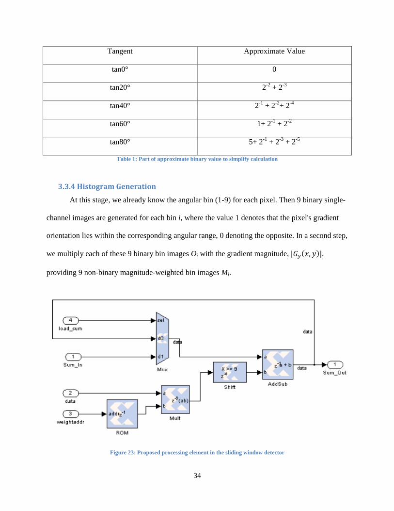
Tangent Approximate Value
tan0° 0
tan20° 2-2
+ 2-3
tan40° 2-1
+ 2-2
+ 2-4
tan60° 1+ 2-1
+ 2-2
tan80° 5+ 2-1
+ 2-3
+ 2-5
Table 1: Part of approximate binary value to simplify calculation
3.3.4 Histogram Generation
At this stage, we already know the angular bin (1-9) for each pixel. Then 9 binary single-
channel images are generated for each bin i, where the value 1 denotes that the pixel's gradient
orientation lies within the corresponding angular range, 0 denoting the opposite. In a second step,
we multiply each of these 9 binary bin images Oi with the gradient magnitude, | ( )|,
providing 9 non-binary magnitude-weighted bin images Mi.
Figure 23: Proposed processing element in the sliding window detector
35
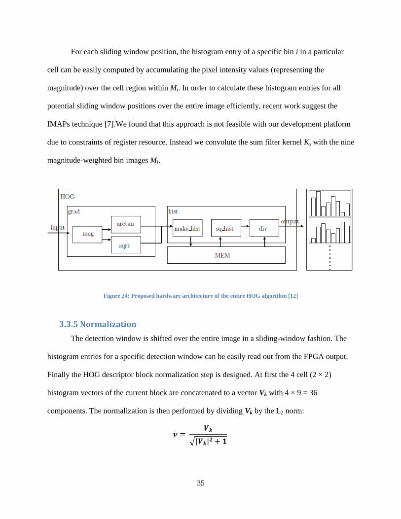
For each sliding window position, the histogram entry of a specific bin i in a particular
cell can be easily computed by accumulating the pixel intensity values (representing the
magnitude) over the cell region within Mi. In order to calculate these histogram entries for all
potential sliding window positions over the entire image efficiently, recent work suggest the
IMAPs technique [7].We found that this approach is not feasible with our development platform
due to constraints of register resource. Instead we convolute the sum filter kernel Ks with the nine
magnitude-weighted bin images Mi.
Figure 24: Proposed hardware architecture of the entire HOG algorithm [12]
3.3.5 Normalization
The detection window is shifted over the entire image in a sliding-window fashion. The
histogram entries for a specific detection window can be easily read out from the FPGA output.
Finally the HOG descriptor block normalization step is designed. At first the 4 cell (2 × 2)
histogram vectors of the current block are concatenated to a vector Vk with 4 × 9 = 36
components. The normalization is then performed by dividing Vk by the L2 norm:
√| |

36
Where Vk is a vector corresponding to a combined histogram for the block, and v is a
normalized vector, which is a final HOG feature. We use a linear SVM (LSVM) for
classification, operating on the normalized HOG feature vectors that are stored line by line in a
matrix. The system can thus parallelize the classification of all windows.
3.4 Evaluation
SVM training is performed using the INRIA dataset [9] that remains one of the widely
used benchmark sets. For the purpose of evaluation. However, a per-window evaluation is
performed. Though in practice, per-window performance measures can fail to predict actual per-
image performance [8].
3.5 Summary
The proposed HOG descriptor computation fits into a Xilinx Zynq-7000 device.
Unfortunately we have to admit that this project is still working in progress. We are unable to
show the result of hardware implementation because the block design of memory controller is
still not finished so that we could not finish the steps of histogram gathering and normalization at
this time. We will keep working on this block design and try to have the whole hardware
architecture completely built and successfully worked next.
Moreover, there is still room to further speed up the framework. Outsourcing further parts
of our recognition framework to the FPGA requires additional resources that are provided by
available extension boards with additional FPGA and RAM. We are working on integrating the
HOG descriptor normalization and linear SVM prediction [10] into the FPGA.

37
Chapter 4: Conclusions and Future Work
In conclusion, this project evaluates the overall accuracy of the HOG algorithm for pedestrian
detection. Our team successfully simulated the algorithm in software and discovered the need for
hardware acceleration. Although hardware acceleration has not been fully realized on an FPGA yet,
it is evident what type of impact this project could have. We expect to see this algorithm incorporated
into an all-encompassing automobile computer vision platform in the near future.

38
References
[1] D. Gavrila, P. Marchal, and M.-M. Meinecke, “SAVE-U, Deliverable1-A: Vulnerable Road
User Scenario Analysis,” technical report, Information Soc. Technology Programme of the EU,
2003.
[2] W. Jones, “Building Safer Cars,” IEEE Spectrum, vol. 39, no. 1,pp. 82-85, Jan. 2002.
[3] N. Dalal and B. Triggs. Histograms of oriented gradients for human detection. In Proc. of the
IEEE International Conference on Computer Vision and Pattern Recognition (CVPR), pages I:
886-893, 2005.
[4] ZC702 Evaluation Board for the Zynq-7000 XC7Z020 All Programmable SoC User Guide,
UG850 (v1.2), Xilinx, April 4, 2013
[5] T. P. Cao and G. Deng. Real-time vision - based stop sign detection system on FPGA. In
Proc. of the International Conference on Digital Image Computing: Techniques and Applications
(DICTA), pages 465-471, IEEE Computer Society, 2008.
[6] Buether, John; Frankfurth, Josh; Lee, Meng-Chiao; Xie, Kan; FPGA Image Processing for
Driver Assistance Camera, 2011.
[7] Q. A. Zhu, M. C. Yeh, K. T. Cheng, and S. Avidan. Fast human detection using a cascade of
histograms of oriented gradients. In Proc. of the IEEE International Conference on Computer
Vision and Pattern Recognition (CVPR), pages II: 1491-1498, 2006.
[8] P. Dollár, C. Wojek, B. Schiele, P. Perona. Pedestrian detection: A benchmark. In Proc. of
the IEEE International Conference on Computer Vision and Pattern Recognition (CVPR), 2009.
[9] INRIA Person Dataset, 2005. http://lear.inrialpes.fr/data/human.

39
[10] K.M. Irick, M. DeBole, V. Narayanan, A. Gayasen. A Hardware Efficient Support Vector
Machine Architecture for FPGA. In Proc. of the IEEE International Symposium on Field-
Programmable Custom Computing Machines (FCCM), pages 304-305, 2008.
[11] Support vector machines: The linearly separable case. Stanford University. Cambridge
Press. http://nlp.stanford.edu/IR-book/html/htmledition/support-vector-machines-the-linearly-
separable-case-1.html. 2008.
[12] Ryoji Kadota, Hiroki Sugano, Masayuki Hiromoto, Hiroyuki Ochi, Ryusuke Miyamoto,
Yukihiro Nakamura, "Hardware Architecture for HOG Feature Extraction," iih-msp, pp.1330-
1333, 2009 Fifth International Conference on Intelligent Information Hiding and Multimedia
Signal Processing, 2009.
[13] Support Vector Machines (SVM). MathWorks Documentation Center.
http://www.mathworks.com/help/stats/support-vector-machines-svm.html.
[14] T. Joachims, 11. Making large-Scale SVM Learning Practical. Advances in Kernel Methods
- Support Vector Learning, B. Schölkopf and C. Burges and A. Smola (ed.), MIT Press, 1999.
[15] G. Bradski. The OpenCV Library. Dr. Dobb’s Journal of Software Tools. 2000.
[16] FMC-IMAGEON Building a Video Design from Scratch Tutorial, Xilinx
40
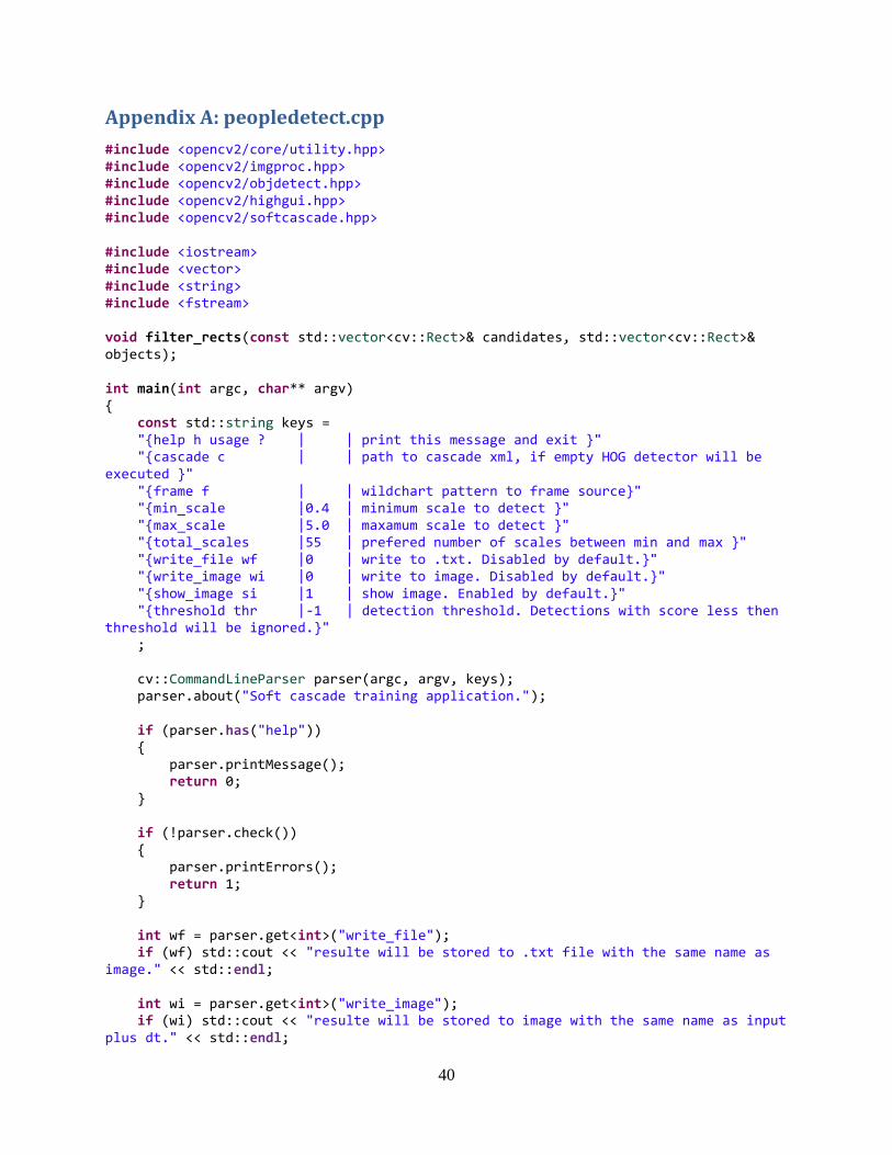
Appendix A: peopledetect.cpp
#include <opencv2/core/utility.hpp> #include <opencv2/imgproc.hpp> #include <opencv2/objdetect.hpp> #include <opencv2/highgui.hpp> #include <opencv2/softcascade.hpp> #include <iostream> #include <vector> #include <string> #include <fstream> void filter_rects(const std::vector<cv::Rect>& candidates, std::vector<cv::Rect>& objects); int main(int argc, char** argv) { const std::string keys = "{help h usage ? | | print this message and exit }" "{cascade c | | path to cascade xml, if empty HOG detector will be executed }" "{frame f | | wildchart pattern to frame source}" "{min_scale |0.4 | minimum scale to detect }" "{max_scale |5.0 | maxamum scale to detect }" "{total_scales |55 | prefered number of scales between min and max }" "{write_file wf |0 | write to .txt. Disabled by default.}" "{write_image wi |0 | write to image. Disabled by default.}" "{show_image si |1 | show image. Enabled by default.}" "{threshold thr |-1 | detection threshold. Detections with score less then threshold will be ignored.}" ; cv::CommandLineParser parser(argc, argv, keys); parser.about("Soft cascade training application."); if (parser.has("help")) { parser.printMessage(); return 0; } if (!parser.check()) { parser.printErrors(); return 1; } int wf = parser.get<int>("write_file"); if (wf) std::cout << "resulte will be stored to .txt file with the same name as image." << std::endl; int wi = parser.get<int>("write_image"); if (wi) std::cout << "resulte will be stored to image with the same name as input plus dt." << std::endl;

41
int si = parser.get<int>("show_image"); float minScale = parser.get<float>("min_scale"); float maxScale = parser.get<float>("max_scale"); int scales = parser.get<int>("total_scales"); int thr = parser.get<int>("threshold"); cv::HOGDescriptor hog; cv::softcascade::Detector cascade; bool useHOG = false; std::string cascadePath = parser.get<std::string>("cascade"); if (cascadePath.empty()) { useHOG = true; hog.setSVMDetector(cv::HOGDescriptor::getDefaultPeopleDetector()); std::cout << "going to use HOG detector." << std::endl; } else { cv::FileStorage fs(cascadePath, cv::FileStorage::READ); if( !fs.isOpened()) { std::cout << "Soft Cascade file " << cascadePath << " can't be opened." << std::endl << std::flush; return 1; } cascade = cv::softcascade::Detector(minScale, maxScale, scales, cv::softcascade::Detector::DOLLAR); if (!cascade.load(fs.getFirstTopLevelNode())) { std::cout << "Soft Cascade can't be parsed." << std::endl << std::flush; return 1; } } std::string src = parser.get<std::string>("frame"); std::vector<cv::String> frames; cv::glob(parser.get<std::string>("frame"), frames); std::cout << "collected " << src << " " << frames.size() << " frames." << std::endl; for (int i = 0; i < (int)frames.size(); ++i) { std::string frame_sourse = frames[i]; cv::Mat frame = cv::imread(frame_sourse); if(frame.empty()) { std::cout << "Frame source " << frame_sourse << " can't be opened." << std::endl << std::flush; continue;

42
} std::ofstream myfile; if (wf) myfile.open((frame_sourse.replace(frame_sourse.end() - 3, frame_sourse.end(), "txt")).c_str(), std::ios::out); //// if (useHOG) { std::vector<cv::Rect> found, found_filtered; // run the detector with default parameters. to get a higher hit-rate // (and more false alarms, respectively), decrease the hitThreshold and // groupThreshold (set groupThreshold to 0 to turn off the grouping completely). hog.detectMultiScale(frame, found, 0, cv::Size(8,8), cv::Size(32,32), 1.05, 2); filter_rects(found, found_filtered); std::cout << "collected: " << (int)found_filtered.size() << " detections." << std::endl; for (size_t ff = 0; ff < found_filtered.size(); ++ff) { cv::Rect r = found_filtered[ff]; cv::rectangle(frame, r.tl(), r.br(), cv::Scalar(0,255,0), 3); if (wf) myfile << r.x << "," << r.y << "," << r.width << "," << r.height << "," << 0.f << "\n"; } } else { std::vector<cv::softcascade::Detection> objects; cascade.detect(frame, cv::noArray(), objects); std::cout << "collected: " << (int)objects.size() << " detections." << std::endl; for (int obj = 0; obj < (int)objects.size(); ++obj) { cv::softcascade::Detection d = objects[obj]; if(d.confidence > thr) { float b = d.confidence * 1.5f; std::stringstream conf(std::stringstream::in | std::stringstream::out); conf << d.confidence; cv::rectangle(frame, cv::Rect((int)d.x, (int)d.y, (int)d.w, (int)d.h), cv::Scalar(b, 0, 255 - b, 255), 2); cv::putText(frame, conf.str() , cv::Point((int)d.x + 10, (int)d.y - 5),1, 1.1, cv::Scalar(25, 133, 255, 0), 1, cv::LINE_AA);
43
if (wf) myfile << d.x << "," << d.y << "," << d.w << "," << d.h << "," << d.confidence << "\n"; } } } if (wi) cv::imwrite(frame_sourse + ".dt.png", frame); if (wf) myfile.close(); if (si) { cv::imshow("pedestrian detector", frame); cv::waitKey(10); } } if (si) cv::waitKey(0); return 0; } void filter_rects(const std::vector<cv::Rect>& candidates, std::vector<cv::Rect>& objects) { size_t i, j; for (i = 0; i < candidates.size(); ++i) { cv::Rect r = candidates[i]; for (j = 0; j < candidates.size(); ++j) if (j != i && (r & candidates[j]) == r) break; if (j == candidates.size()) objects.push_back(r); } }
44
Appendix B: videostream.cpp
#include <iostream>
#include <opencv2/opencv.hpp>
using namespace std;
using namespace cv;
int main (int argc, const char * argv[])
{
VideoCapture cap(CV_CAP_ANY);
if (!cap.isOpened())
return -1;
Mat img;
namedWindow("video capture", CV_WINDOW_AUTOSIZE);
while (true)
{
cap >> img;
imshow("video capture", img);
if (waitKey(10) >= 0)
break;
}
return 0;
}
45
Appendix C: videopeopledetect.cpp
#include <iostream> #include <opencv2/opencv.hpp> using namespace std; using namespace cv; int main (int argc, const char * argv[]) { VideoCapture cap(CV_CAP_ANY); cap.set(CV_CAP_PROP_FRAME_WIDTH, 1.3*320); cap.set(CV_CAP_PROP_FRAME_HEIGHT, 1.3*240); if (!cap.isOpened()) return -1; Mat img; HOGDescriptor hog; hog.setSVMDetector(HOGDescriptor::getDefaultPeopleDetector()); namedWindow("video capture", CV_WINDOW_AUTOSIZE); while (true) { cap >> img; if (!img.data) continue; vector<Rect> found, found_filtered; hog.detectMultiScale(img, found, 0, Size(8,8), Size(32,32), 1.05, 2); size_t i, j; for (i=0; i<found.size(); i++) { Rect r = found[i]; for (j=0; j<found.size(); j++) if (j!=i && (r & found[j])==r) break; if (j==found.size()) found_filtered.push_back(r); } for (i=0; i<found_filtered.size(); i++) { Rect r = found_filtered[i]; r.x += cvRound(r.width*0.1); r.width = cvRound(r.width*0.8); r.y += cvRound(r.height*0.06); r.height = cvRound(r.height*0.9); rectangle(img, r.tl(), r.br(), cv::Scalar(0,255,0), 2); } imshow("video capture", img); if (waitKey(20) >= 0) break; } return 0; }

46
Appendix D: 1framepeopledetect.cpp
#include "opencv2/imgproc/imgproc.hpp" #include "opencv2/objdetect/objdetect.hpp" #include "opencv2/highgui/highgui.hpp" #include <stdio.h> #include <string.h> #include <ctype.h> using namespace cv; using namespace std; int main(int argc, char** argv) { Mat img; FILE* f = 0; char _filename[1024]; if( argc == 1 ) { printf("Usage: peopledetect (<image_filename> | <image_list>.txt)\n"); return 0; } img = imread(argv[1]); if( img.data ) { strcpy(_filename, argv[1]); } else { f = fopen(argv[1], "rt"); if(!f) { fprintf( stderr, "ERROR: the specified file could not be loaded\n"); return -1; } } HOGDescriptor hog; hog.setSVMDetector(HOGDescriptor::getDefaultPeopleDetector()); namedWindow("people detector", 1); for(;;) { char* filename = _filename; if(f) { if(!fgets(filename, (int)sizeof(_filename)-2, f)) break; //while(*filename && isspace(*filename)) // ++filename; if(filename[0] == '#') continue;

47
int l = (int)strlen(filename); while(l > 0 && isspace(filename[l-1])) --l; filename[l] = '\0'; img = imread(filename); } printf("%s:\n", filename); if(!img.data) continue; fflush(stdout); vector<Rect> found, found_filtered; double t = (double)getTickCount(); // run the detector with default parameters. to get a higher hit-rate // (and more false alarms, respectively), decrease the hitThreshold and // groupThreshold (set groupThreshold to 0 to turn off the grouping completely). hog.detectMultiScale(img, found, 0, Size(8,8), Size(32,32), 1.05, 2); t = (double)getTickCount() - t; printf("tdetection time = %gms\n", t*1000./cv::getTickFrequency()); size_t i, j; for( i = 0; i < found.size(); i++ ) { Rect r = found[i]; for( j = 0; j < found.size(); j++ ) if( j != i && (r & found[j]) == r) break; if( j == found.size() ) found_filtered.push_back(r); } for( i = 0; i < found_filtered.size(); i++ ) { Rect r = found_filtered[i]; // the HOG detector returns slightly larger rectangles than the real objects. // so we slightly shrink the rectangles to get a nicer output. r.x += cvRound(r.width*0.1); r.width = cvRound(r.width*0.8); r.y += cvRound(r.height*0.07); r.height = cvRound(r.height*0.8); rectangle(img, r.tl(), r.br(), cv::Scalar(0,255,0), 3); } imshow("people detector", img); int c = waitKey(0) & 255; if( c == 'q' || c == 'Q' || !f) break; } if(f) fclose(f); return 0; }
48
Appendix E: HOG Top Module
`timescale 1ns / 1ps
module hog(
input clk,
input rst,
input [1:0] x,
input [1:0] y,
output [3:0] n,
inout [13:0] ram_data,
output ram_clk,
output adv,
output ce,
output oe,
output we,
output lb,
output ub,
output cre,
output [32:0] norm_all);
wire [9:0] m_xy;
wire [7:0] direc;
wire s;
gradient
hog1(.clk(clk),.rst(rst),.x(x),.y(y),.m_xy(m_xy),.direc(direc),.n(n),.
s(s));
top_histogram
hog2(.clk(clk),.rst(rst),.m_xy(m_xy),.direc(direc),.ram_data(ram_data)
,
.ram_clk(ram_clk),.adv(adv),.ce(ce),.oe(oe),.we(we),.lb(lb),.ub(ub),
.cre(cre),.norm_all(norm_all));
endmodule

49
Appendix F: Gradient Calculating Top Module
`timescale 1ns / 1ps
module gradient(
input clk,
input rst,
input [1:0] x,
input [1:0] y,
output [9:0] m_xy,
output [7:0] direc,
output [3:0] n,
output s);
wire [8:0] f_x,f_y;
calculate grad1(.x(x),.y(y),.f_x(f_x),.f_y(f_y));
magnitude grad2(.f_x(f_x),.f_y(f_y),.m_xy(m_xy));
direction
grad3(.f_x(f_x),.f_y(f_y),.clk(clk),.rst(rst),.direc(direc),.n(n),.s(s
));
endmodule
50
Appendix G: Gradient First Derivative Calculating Module
`timescale 1ns / 1ps
module calculate(
input [1:0] x,
input [1:0] y,
output [8:0] f_x,
output [8:0] f_y);
wire [8:0] f1,f2,f3,f4;
wire [1:0] x1,x2,y1,y2;
assign x1= x+1'b1; // x1=x+1
assign x2= x-1'b1; // x2=x-1
assign y1= y+1'b1; // y1=y+1
assign y2= y-1'b1; // x2=y-1
lumin c1(.x(x1),.y(y),.f_xy(f1)); // f1= f(x+1,y)
lumin c2(.x(x2),.y(y),.f_xy(f2)); // f2= f(x-1,y)
lumin c3(.x(x),.y(y1),.f_xy(f3)); // f3= f(x,y+1)
lumin c4(.x(x),.y(y2),.f_xy(f4)); // f4= f(x,y-1)
assign f_x = f1-f2; //fx = f(x+1,y) - f(x-
1,y)
assign f_y = f3-f4; //fy = f(x,y+1) - f(x,y-
1)
endmodule

51
Appendix H: Luminous Input Module
`timescale 1ns / 1ps
module lumin(
input [1:0] x,
input [1:0] y,
output [8:0] f_xy);
assign f_xy = (x==2'b10)&&(y == 2'b10) ? 9'd56 :
9'd0;
endmodule

52
Appendix I: Gradient Direction Calculating Module
`timescale 1ns / 1ps
module direction(
input [8:0] f_x,
input [8:0] f_y,
input clk,
input rst,
output reg [7:0] direc,
output reg [3:0] n,
output s);
reg [3:0] i=1;
reg [5:0] tani;
wire [14:0] mult;
assign mult = f_x*tani;
always@(posedge clk)
begin
if(rst)
begin
i <= 4'b0000;
s <= 1'b0;
end
else if(i == 4'b1001)
i <= 4'b0000;
else if(f_y <= mult[14:6])
begin
i <=i+1'b1;
s <= 1'b0;
end
else
begin
n <=i;
s <= 1'b1;
i <= 4'b0000;
end
end
always@(i)
begin
case(i)
4'd1 : tani = {3'b110,3'b011};
//tan112.5=-2.42 bin=5
4'd2 : tani = {3'b101,3'b000}; //tan135=-
1 bin=6
4'd3 : tani = {3'b100,3'b011};
//tan157.5=-0.42 bin=7
4'd4 : tani = {3'b000,3'b000}; //tan180=0
bin=8
53
4'd5 : tani = {3'b000,3'b011};
//tan22.5=0.42 bin=1
4'd6 : tani = {3'b001,3'b000}; //tan45=1
bin=2
4'd7 : tani = {3'b010,3'b011};
//tan67.5=2.42 bin=3
4'd8 : tani = {3'b011,3'b111}; //tan90=
infinity bin=4
default : tani = 6'b1;
endcase
end
always@(n)
begin
case(n) //match with the average direction angel
4'd1 : direc = 8'd101;
4'd2 : direc = 8'd124;
4'd3 : direc = 8'd146;
4'd4 : direc = 8'd169;
4'd5 : direc = 8'd11;
4'd6 : direc = 8'd68;
4'd7 : direc = 8'd56;
4'd8 : direc = 8'd79;
default : direc = 8'b1;
endcase
end
endmodule

54
Appendix J: Gradient Magnitude Calculating Module (LUT)
`timescale 1ns / 1ps
module magnitude(
input [8:0] f_x,
input [8:0] f_y,
output reg [9:0] m_xy);
reg [7:0] f_x1;
reg [7:0] f_y1;
wire [16:0] xy={f_x1,f_y1};
always@(f_x,f_y,xy)
begin
f_x1 = f_x[7:0];
f_y1 = ~(f_y-1'b1);
case(xy)
1 : m_xy= 9'd0 ;
2 : m_xy= 9'd1 ;
3 : m_xy= 9'd2 ;
4 : m_xy= 9'd3 ;
5 : m_xy= 9'd4 ;
6 : m_xy= 9'd5 ;
7 : m_xy= 9'd6 ;
8 : m_xy= 9'd7 ;
9 : m_xy= 9'd8 ;
10 : m_xy= 9'd9 ;
…

55
Appendix K: Histogram Top Module
`timescale 1ns / 1ps
module top_histogram(
input clk,
input rst,
input s,
input [9:0] m_xy,
input [7:0] direc,
inout [13:0] ram_data,
output ram_clk,
output adv,
output ce,
output oe,
output we,
output lb,
output ub,
output cre,
output [32:0] norm_all,
output [25:0] ram_address);
reg [3:0] n;
wire [13:0] hist;
wire [13:0] norm;
histogram
top1(.clk(clk),.rst(rst),.m_xy(m_xy),.direc(direc),.n(n),.hist(hist));
store
top2(.clk(clk),.rst(rst),.hist(hist),.n(n),.norm(norm),.ram_data(ram_d
ata),
.ram_clk(ram_clk),.adv(adv),.ce(ce),.oe(oe),.we(we),.lb(lb),.ub(u
b),.cre(cre),
.ram_address(ram_address),.s(s));
normalization
top3(.clk(clk),.rst(rst),.norm(norm),.norm_all(norm_all));
endmodule

56
Appendix L: Histogram Block Module
`timescale 1ns / 1ps
module histogram(
input clk,
input rst,
input [9:0] m_xy,
input [7:0] direc,
input [3:0] n,
output [13:0] hist);
parameter [3:0] a ={1'b0,3'b011}; // put the value
as the constant 0.4 (0.375)
reg [13:0] vote0;
reg [13:0] vote1;
wire [14:0] vote;
always@(posedge clk)
begin
if(rst)
begin
vote0 <= 14'b0;
vote1 <= 14'b0;
end
else
begin
vote0 <= (4'b1-a)*m_xy; //integer 11 bits
fraction 3 bits
vote1 <= a*m_xy;
end
end
assign vote = vote0 + vote1;
assign hist = vote[14:1]; //get the average of
vote value 3bits of fraction
endmodule

57
Appendix M: Normalization Block Module
`timescale 1ns / 1ps
module normalization(
input clk,
input rst,
input [13:0] norm, //14bits 3bits of fraction
output [32:0] norm_all);
reg [3:0] count=0;
reg []
always@(posedge clk)
begin
count <=count+1'b1;
if(count == 3'b1001)
begin
count <= 4'b0;
end
case(count)
4'b0000: ;
4'b0001: ;
4'b0010: ;
4'b0011: ;
4'b0100: ;
4'b0101: ;
4'b0110: ;
4'b0111: ;
endcase
end
endmodule

58
Appendix N: SRAM Controller Module
`timescale 1ns / 1ps
module sram_control(
input [13:0] datawrite,
output [13:0] dataread,
inout [13:0] ram_data,
input fpga_clk,
input [25:0] fpga_address,
output [25:0] ram_address,
input start,
input fpga_ctl,
output ram_clk,
output adv,
output ce,
output oe,
output we,
output lb,
output ub,
output cre);
reg [13:0] data;
reg [25:0] address;
reg [3:0] count=0;
reg ctl;
reg busy =1'b0;
//////////////////////////////////////////////////////////////
// control the sram to make it have two model: read and write
///////////////////////////////////////////////////////////////
assign ram_clk = 1'b0;
assign lb = 1'b0;
assign ub = 1'b0;
assign ce = 1'b0;
assign oe = 1'b0;
assign we = ctl;
assign cre = 1'b0;
assign adv = 1'b0;
assign dataread = data;
assign ram_address = address;
assign ram_data = ctl ? 14'bz : data;
//////////////////////////////////////////////////////////////////////
//////////
//when ctl = 1 , sram in the read model ,when ctl =0 sram in the write
model
//////////////////////////////////////////////////////////////////////
///////////
always@(posedge fpga_clk)
begin
if(busy == 1'b0)
begin
ctl <= fpga_ctl;
count <= 0;

59
if(start == 1)
begin
busy <= 1'b1;
data <= ctl ?
ram_data : datawrite;
address <=
fpga_address;
end
end
else
if(count == 9)
busy <= 1'b0;
else
count <= count +1'b1;
end
endmodule
60
Appendix O: Histogram Storing Module
`timescale 1ns / 1ps
module store(
input clk,
input rst,
input [13:0] hist,
input [3:0] n,
input s,
output [13:0] norm,
inout [13:0] ram_data,
output ram_clk,
output adv,
output ce,
output oe,
output we,
output lb,
output ub,
output cre,
output [25:0] ram_address);
reg fpga_ctl=1'b1;
reg start;
reg [25:0] fpga_address;
sram_control
store1(.fpga_clk(clk),.datawrite(hist),.dataread(norm),.ram_data(ram_d
ata),.fpga_address(fpga_address),
.ram_address(ram_address),.start(start),.fpga_ctl(fpga_ctl),.ram_
clk(ram_clk),.adv(adv),.ce(ce),.oe(oe),.we(we),
.lb(lb),.ub(ub),.cre(cre));
always@(posedge clk)
begin
if(rst)
begin
fpga_ctl <= 1'b0;
start <= 1'b0;
end
else
begin
if(s == 1'b1)
begin
start <= 1'b1;
fpga_ctl <= 1'b0;
fpga_address <=
fpga_address +1'b1;
end
else
begin
61
start <= 1'b0;
end
end
end
endmodule