tools and techniques for considering transmission … and techniques for considering transmission...

Tools and Techniques for ConsideringTransmission Corridor Optionsto Accommodate Large ScaleRenewable Energy Resources

Final Project Report

Power Systems Engineering Research Center

Empowering Minds to Engineerthe Future Electric Energy System

Tools and Techniques for Considering Transmission Corridor Options to Accommodate

Large Scale Renewable Energy Resources

Final Project Report

Project Team

Vijay Vittal, Gerald T. Heydt Sruthi Hariharan, Samir Gupta

Arizona State University

Gabriela Hug, Rui Yang, Amritanshu Pandey, Harald Franchetti Carnegie Mellon University

PSERC Publication 12-23

August 2012

For information about this project contact: Vijay Vittal Arizona State University School of Electrical, Computer and Energy Engineering PO Box 875706 Tempe, AZ 85257-5706 [email protected] (480) 965-1879 Power Systems Engineering Research Center The Power Systems Engineering Research Center (PSERC) is a multi-university Center conduct-ing research on challenges facing the electric power industry and educating the next generation of power engineers. More information about PSERC can be found at the Center’s website: http://www.pserc.org. For additional information, contact: Power Systems Engineering Research Center Arizona State University 527 Engineering Research Center Tempe, Arizona 85287-5706 Phone: 480-965-1643 Fax: 480-965-0745 Notice Concerning Copyright Material PSERC members are given permission to copy without fee all or part of this publication for in-ternal use if appropriate attribution is given to this document as the source material. This report is available for downloading from the PSERC website.

2012 Arizona State University. All rights reserved.

i

Acknowledgements

This is the final report for the Power Systems Engineering Research Center (PSERC) research project titled “Tools and Techniques for Considering Transmission Corridor Options to Accom-modate Large Scale Renewable Energy Resources” (PSERC Project S-41). We express our ap-preciation for the support provided by PSERC’s industrial members and by the National Science Foundation under the Industry / University Cooperative Research Center program. We wish to thank the following industry advisors for their input and guidance during the project:

Brian Keel – Salt River Project

Eugene Litvinov – ISO-New England

Doug McLaughlin – Southern Company

Mahendra Patel – PJM Interconnection

Jon Stahlhut – Arizona Public Service Co.

The authors also express appreciation for the supplemental support provided by the SRC Smart Grid Research Center and the BPA Technology Innovation Program.

ii

Executive Summary

The increase in economic and environmental concerns has resulted in the fast growth of renewa-ble resource penetration in the electric power grid. In order to ensure increased penetration of renewable resources several states have a mandated renewable portfolio standard (RPS) which requires a certain percentage of the load to be served by renewable resources. The RPS also states by which year the standard has to be met. In California, for example, the RPS requirement is 20% by the year 2012 and 33% by the year 2020. This project addresses three important as-pects of integrating renewable resources in the bulk power system:

1. Transmission expansion planning including renewable resources

2. Impact of large scale energy storage

3. The impact of flexible AC transmission systems (FACTS)

Each of these three aspects is discussed in separate parts of the report. A summary related to each aspect is presented below.

Part 1: Transmission Expansion Planning Including Renewable Resources Due to economic and environmental reasons, several states in the United States of America have a mandated renewable portfolio standard which requires that a certain percentage of the load served has to be met by renewable resources of energy such as solar, wind and biomass. Renewable resources provide energy at a low variable cost and produce less greenhouse gases as compared to conventional generators. However, some of the complex issues with renewable resource integration are due to their intermittent and non-dispatchable characteristics. Furthermore, most renewable resources are location constrained and are usually located in regions with insufficient transmission facilities. In order to deal with the challenges presented by renewable resources as compared to conventional resources, the transmission network expansion planning procedures need to be modified. New high voltage lines need to be constructed to connect the remote renewable resources to the existing transmission network to serve the load centers. Moreover, the existing transmission facilities may need to be reinforced to accommodate the large scale penetration of renewable resource.

This part of the report proposes a methodology for transmission expansion planning with large-scale integration of renewable resources, mainly solar and wind generation. An optimization model is used to determine the lines to be constructed or upgraded for several scenarios of vary-ing levels of renewable resource penetration. The various scenarios to be considered are obtained from a production cost model that analyses the effects that renewable resources have on the transmission network over the planning horizon. A realistic test bed was created using the data for solar and wind resource penetration in the state of Arizona. The results of the production cost model and the optimization model were subjected to tests to ensure that the North American Electric Reliability Corporation (NERC) mandated N-1 contingency criterion is satisfied. Fur-thermore, a cost versus benefit analysis was performed to ensure that the proposed transmission plan is economically beneficial.

Different planning methods and models are used by the power industry to plan transmission for renewable resources. For example, the Midwest ISO mainly uses a power flow tool for transmis-sion expansion planning with renewable resources. In order to ensure reliability of the proposed

iii

expansion plan dynamic simulations, voltage stability and small signal oscillation analysis tools are also employed. The transmission planning process for renewable resources employed at the Midwest ISO can be summarized as follows:

a) Renewable resource forecasting and placement in power flow models

b) Copper sheet analysis (power flow with no limits on transmission capacity) to identify a preliminary transmission plan. This preliminary plan is supplemented with area based con-tour plots that take into consideration areas lacking in transmission facilities that do not show up in the copper sheet analysis.

c) Use production cost model to identify an expansion plan.

d) Perform reliability assessment and a cost versus benefit analysis for the proposed set of transmission paths to come up with a consolidated transmission plan.

The main tool used for transmission planning for large scale renewable resource integration, as proposed in this part of the report, is a linear, mixed-integer optimization model which is based on the DC optimal power flow formulation. The optimization model includes a time variable that is used to account for the hourly and seasonal fluctuations in renewable energy availability. However, given the complexity of the power grid and the time horizon of transmission planning, it is proposed that rather than using the entire planning horizon data, a few scenarios be selected to be input to the optimization model. These scenarios are selected using a production cost model which identifies weeks within the planning horizon with increased renewable energy availability. The optimization model is run for each of the scenarios identified and a corresponding optimal set of transmission paths to be constructed is obtained. The results of the optimization model are then combined to form a comprehensive transmission expansion plan, which in turn needs to be checked for economic benefits as well as reliability over the entire planning horizon.

Part 2: Power Flow Control and Probabilistic Load Flow The existing electric power grid was built for a situation in which power was injected at a few locations by dispatchable bulk power plants to supply inflexible loads. It was designed for reoc-curring power flow patterns and has limited control capabilities. In the meantime, the increased consumption, the liberalization of electricity markets and the increase in variable renewable gen-eration have led to a situation in which the constraints imposed by the transmission grid result in economically suboptimal generation dispatches to avoid overloads in the system. However, it often is not just a matter of insufficient transmission line capacities but because power flows are governed by Kirchhoff’s Laws a single line reaching its limit restricts how the entire system is operated. To enable the transition to an efficient sustainable electric energy supply system, the transmission grid needs to be able to adjust to the increasingly varying power flows. Power flow control enabled for example by FACTS devices provides the opportunity to influence where power is flowing and therefore to improve the usage of the existing transmission system for varying generation in-feeds.

In this part of the project, the focus is on using power flow control to enable a flexible transmis-sion grid. The work includes (1) the derivation of a decentralized control scheme to determine the optimal steady-state settings of power flow control devices in order to fully utilize the exist-ing transmission infrastructures and (2) an analysis of the flexibility achieved in the transmission

iv

grid. The control approach is a two-stage algorithm based on regression analysis: in the offline stage, a regression function is determined which gives the optimal device setting as a function of a few key measurements in the system. In the online stage, the regression function and the values of the key measurements can be used to locally determine the optimal setting of the device with-out carrying out the optimal power flow calculation. The method is tested for thyristor-controlled series compensators in the IEEE 14 bus system. The analysis of the flexibility achieved by these devices includes the consideration of the improvement of the transmission capacity usage and the increased range of possible generation dispatches.

Another aspect considered in this part of the project corresponds to probabilistic load flow calcu-lations. The probabilistic nature of variable renewable generation has led to the introduction of probabilistic load flow calculations which are based on probability distributions of the renewable generation output. While probability distributions for wind generation are available, they do not provide information about the correlation between the in-feeds of power generation from two not co-located wind plants. Hence, a further contribution of this work is an initial study on how to mathematically model two β-distributions with a specific correlation.

Part 3: Large Scale Energy Storage

This part of the project technical report concerns the impact of large scale energy storage on in-terconnected electric power systems, especially systems with high penetration of renewable en-ergy generation. The rapidly increasing integration of renewable energy source into the grid is driving greater attention towards electrical energy storage systems which can serve many appli-cations like economically meeting peak loads, providing spinning reserve. Economic dispatch is performed with bulk energy storage with wind energy penetration in power systems allocating the generation levels to the units in the mix, so that the system load is served and most economi-cally. The results obtained in previous research to solve for economic dispatch uses a linear cost function for a Direct Current Optimal Power Flow (DCOPF). This report uses quadratic cost function for a DCOPF implementing quadratic programming (QP) to minimize the function. A Matlab program was created to simulate different test systems including an equivalent section of the WECC system, namely for Arizona, summer peak 2009.

A mathematical formulation of a strategy of when to charge or discharge the storage is incorpo-rated in the algorithm. In this report various test cases are shown in a small three bus test bed and also for the state of Arizona test bed. The main conclusions drawn from the two test beds is that the use of energy storage minimizes the generation dispatch cost of the system and benefits the power system by serving the peak partially from stored energy. It is also found that use of energy storage systems may alleviate the loading on transmission lines which can defer the upgrade and expansion of the transmission system.

v

Project Publications: G. Heydt. “The Next Generation of Power Distribution Systems.” IEEE Transactions on Smart Grid, v. 1, No. 3, December, 2010, pp. 225 – 235. G. Heydt. Smart Grids: Infrastructure, Technology and Solutions. Stuart Borlaise editor, Chapter 4, “Smart Grid Barriers and Critical Success Factors,” CRC Press, Taylor and Francis Book Co. New York, 2012 Rui Yang, Gabriela Hug. “Optimal Usage of Transmission Capacity with FACTS Devices in the Presence of Wind Generation: A Two-Stage Approach.” PES General Meeting, San Diego, USA, 2012. Rui Yang, Gabriela Hug. “Regression-based FACTS Control for Optimal Usage of Trans-mission Capacity.” TechCon Conference, Austin, 2012.

Student Theses: Harald Franchetti. Probabilistic Load Flow for Correlated Wind Power Outputs. Masters thesis in the process of being completed. Anticipated completion and graduation from TU Vien-na, December 2012. Samir Gupta. Dispatch of Bulk Energy Storage in Power Systems with Wind Generation. MSEE Thesis, Arizona State University, Tempe, AZ, April, 2012. Sruthi Hariharan. Transmission Expansion Planning with Large Scale Renewable Resource Inte-gration. Arizona State University, MS Thesis, May 2012.

Part 1

Transmission Expansion Planning with Large Scale Renewable Resource Integration

Authors

Vijay Vittal Sruthi Hariharan, M.S. Student


For information about Part 1, contact: Vijay Vittal Arizona State University School of Electrical, Computer and Energy Engineering PO Box 875706 Tempe, AZ 85257-5706 [email protected] (480) 965-1879 Power Systems Engineering Research Center The Power Systems Engineering Research Center (PSERC) is a multi-university Center conduct-ing research on challenges facing the electric power industry and educating the next generation of power engineers. More information about PSERC can be found at the Center’s website: http://www.pserc.org. For additional information, contact: Power Systems Engineering Research Center Arizona State University 527 Engineering Research Center Tempe, Arizona 85287-5706 Phone: 480-965-1643 Fax: 480-965-0745 Notice Concerning Copyright Material PSERC members are given permission to copy without fee all or part of this publication for in-ternal use if appropriate attribution is given to this document as the source material. This report is available for downloading from the PSERC website.


i

Table of Contents

1 Introduction ................................................................................................................... 1

1.1 Motivation ............................................................................................................ 1

1.2 Research objectives .............................................................................................. 1

1.3 Organization of the report .................................................................................... 1

2 Literature review ........................................................................................................... 3

2.1 Transmission planning methods proposed in literature ........................................ 3

2.2 Specialized planning algorithms for renewable resource integration ................... 4

2.3 Software tools ....................................................................................................... 4

2.3.1 AMPL ............................................................................................................ 4

2.3.2 MATLAB ...................................................................................................... 5

2.3.3 PowerWorld .................................................................................................. 5

2.3.4 PROMOD ...................................................................................................... 5

2.3.5 PSLF .............................................................................................................. 6

3 Locating renewable generation in WECC .................................................................... 7

4 Proposed transmission planning procedure .................................................................. 9

4.1 Step 1: Locating renewable resources .................................................................. 9

4.2 Step 2: Production cost modeling ......................................................................... 9

4.3 Step 3: Optimization model ................................................................................ 10

4.4 Step 4: Test to ensure N-1 reliability .................................................................. 10

4.5 Step 5: Cost versus benefit analysis ................................................................... 11

4.6 Summary of transmission planning procedure ................................................... 12

5 Optimization model .................................................................................................... 13

5.1 Optimization formulations for TEP .................................................................... 13

5.2 Optimization model details ................................................................................. 17

5.2.1 Input to the optimization model .................................................................. 17

5.2.2 Decision variables ....................................................................................... 18

5.2.3 Objective function ....................................................................................... 18

5.2.4 Constraints ................................................................................................... 20

5.2.5 Output of optimization model ..................................................................... 21

ii

Table of Contents (continued)

6 Realistic test bed ......................................................................................................... 22

6.1 Step 1: Creation of a realistic test bed ................................................................ 22

6.2 Step 2: Production cost modeling ....................................................................... 23

6.3 Step 3 Optimization model ................................................................................. 25

6.4 Step 4: N-1 contingency criterion compliance ................................................... 26

6.5 Step 5: Cost versus benefit analysis ................................................................... 27

7 Conclusion and future work ........................................................................................ 29

References ......................................................................................................................... 31

Appendix A: Test systems data ........................................................................................ 34

A.1: Bus test system .................................................................................................... 34

A.2: 14 Bus test system ............................................................................................... 36

A.3: 118 Bus test system ............................................................................................. 38

Appendix B: Generation interconnection queues ............................................................ 51

Appendix C: Contour plots of CLMP .............................................................................. 52

Appendix D: Optimization model input data ................................................................... 54

iii

List of Figures

Figure 1: Western Electricity Coordinating Council region [22] .................................................. 7

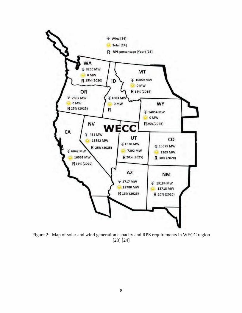
Figure 2: Map of solar and wind generation capacity and RPS requirements in WECC region ... 8

Figure 3: PowerWorld simulator screen shot of the WECC system one-line diagram ................. 9

Figure 4: Summary of proposed transmission planning procedure ............................................. 12

Figure 5: Garver's 6 bus test system ............................................................................................ 15

Figure 6: One line diagram of IEEE 14 bus test system .............................................................. 16

Figure 7: Equivalent test system (AZ) in PowerWorld ............................................................... 22

Figure 8: CLMP contour plot for Scenario 1 ............................................................................... 23

Figure 9: CLMP contour plot for Scenario 2 ............................................................................... 24

Figure 10: CLMP contour plot for Scenario 3 ............................................................................. 24

Figure 11: CLMP contour plot for Scenario 4 ............................................................................. 25

Figure 12: Week 1 of 2020 .......................................................................................................... 52

Figure 13: Week 8 of 2020 .......................................................................................................... 52

Figure 14: Week 23 of 2020 ........................................................................................................ 53

Figure 15: Week 46 of 2020 ........................................................................................................ 53

iv

List of Tables

Table 1: TEP Optimization model results for the 6 bus test system ............................................ 15

Table 2: TEP Optimization model results for the 14 bus test system .......................................... 16

Table 3: TEP Optimization model results for the 118 bus test system ........................................ 17

Table 4: Input to the optimization model ..................................................................................... 18

Table 5: System parameters of the AZ test bed ........................................................................... 22

Table 6: Renewable resource integration in test system .............................................................. 23

Table 7: Optimization model results for all scenarios considered ............................................... 26

Table 8: Comprehensive transmission expansion plan for the realistic test bed ......................... 26

Table 9: Comparative study of output of optimizatio model before and after the construction of lines proposed ................................................................................................................ 27

Table 10: 6 Bus test system bus data ........................................................................................... 34

Table 11: 6 Bus test system branch data ...................................................................................... 35

Table 12: 14 Bus test system bus data ......................................................................................... 36

Table 13: 14 Bus test system branch data .................................................................................... 37

Table 14: 118 Bus test system bus data ....................................................................................... 38

Table 15: 118 Bus test system branch data .................................................................................. 41

Table 16: APS and SRP generation interconnection queue ......................................................... 51

Table 17: Operational cost of generators based on fuel type ....................................................... 54

Table 18: Transmission line construction costs ........................................................................... 54

v

Nomenclature

branch_xij

CG CT

Reactance of branch between bus i and bus j Generator cost function Scaled transmission line construction cost

cij Coefficient corresponding to the ith decision variable (general representa-tion of the objective function),

CLMP Congestion component of the location marginal price DC Direct current ELMP Energy component of the location marginal price F Fixed cost of generator fij Line flow from bus i to bus j in the DC formulation fx Latitude of bus f fy Longitude of bus f Gij Conductance of the line between bus i and bus j ISO Independent systems operator Lj Load at bus j Lft Length of line from bus f to bus t LLMP Loss component of the location marginal price LMP M

Location marginal price A very large number

n Number of sub-periods to consider within a year for planning NERC North American Electric Reliability Corporation NPV Net present value (cost of constructing the transmission line) Pij Real power flow from bus i to bus j Pmin, Pmax Minimum and maximum capacity of generator PV Photovoltaic Qij Reactive power flow from bus i to bus j r Annual rate of interest RPS Renewable portfolio standard tx Latitude of bus t ty Longitude of bus t TEP Transmission expansion planning VOM Variable cost coefficient Vi Voltage magnitude at bus i WECC Western Electricity Coordinating Council WREZ Western Renewable Energy Zones x Binary variable to decide if a line should be added to a right of way

vi

Nomenclature (continued)

Xi Decision variable (general representation of constraints and objective function)

xij Reactance of line between bus i and bus j y Typical life time of transmission line, usually 25-30 years θi Voltage angle at bus i θij θi - θj

1

1 Introduction

1.1 Motivation

Over the last decade, the increase in economic and environmental concerns has resulted in the fast growth of renewable resource penetration in the electric power grid. In order to ensure increased penetration of renewable resources several states have a mandated renewable portfolio standard (RPS) which requires a certain percentage of the load to be served by renewable resources. The RPS also states by which year the standard has to be met. In California, for example, the RPS requirement is 20% by the year 2012 and 33% by the year 2020 [1]. As a result of accelerated increase of renewable resource development, there is a need for sufficient transmission facilities to deliver this renewable energy to the load centers.

Transmission expansion planning (TEP) addresses the problem of expanding an existing transmission network to serve load centers subject to a set of economic and technical constraints. The problem of insufficient export capability of the transmission system could occur for any type of generation interconnected to the grid. However, the variable and intermittent nature of renewable resources would affect the transmission expansion planning procedure. Hence, the inclusion of renewable resources needs to be treated differently as compared to conventional sources of energy while upgrading the transmission system over the planning horizon. Furthermore, there is a significant variation in the available renewable energy, especially solar and wind energy over a year’s time period.

Taking into consideration this intermittent nature of renewable resources, a procedure for transmission expansion planning has been developed in this report. The procedure was tested using a realistic test bed created with the renewable resource information for the state of Arizona, USA.

1.2 Research objectives

The main objectives of this report on TEP for large scale renewable resource penetration are:

• To identify locations that have already been projected for likely development of large scale renewable resources in the Western Electricity Coordinating Council (WECC) region of the USA.

• To develop a system theoretic basis for the identification of new transmission corridors to accommodate these large scale renewable energy resources.

• To develop a realistic test bed to test the proposed planning procedure.

1.3 Organization of the report

The principal contents of the report are developed in 7 chapters and one supplemental section. Chapter 1 presents an overview of the motivation for the study and the study objectives. Chapter 2 presents a literature review of pertinent topics that include previously proposed TEP methods,

2

renewable resource integration, and a brief introduction of the various software tools used in this report. Chapter 3 deals with the identification of locations in the WECC region that have been projected for likely development of large scale renewable energy resources, with a focus on wind and solar resources. Chapter 4 outlines the specialized TEP procedure proposed and discusses the various steps involved in the same. Chapter 5 deals with the optimization model proposed to determine the most economical and feasible set of lines to be included in the grid to best accommodate the renewable resources. The realistic test bed created for the purpose of testing the TEP procedure is discussed in Chapter 6 along with the results of the simulations and studies for the test bed. The required reliability test and a cost versus benefit analysis are also discussed in Chapter 6. Finally, suitable conclusions of the research work are drawn in Chapter 7 along with the scope for future work in this field.

3

2 Literature review

2.1 Transmission planning methods proposed in literature

Transmission planning models can be broadly classified into optimization models, heuristic models, or a combination of these two types of models [2]. The formulation of the optimization model includes an objective function, which needs to be either minimized or maximized while ensuring that the constraint equations of the model are not violated. In the case of TEP, the objective is usually to minimize the sum of the cost of construction of new lines, the cost of reinforcing existing transmission lines and the operational costs of generators over the planning horizon. The constraint equations of the optimization model ensure that the system is modeled in compliance with the power flow equations and operates reliably.

The main mathematical optimization formulations used for transmission planning are the transportation model, the DC model, the AC model, or a hybrid of these three models [3]. The AC model is the most accurate representation of the system as it models reactive power calculations and system losses, which the other two formulations do not model these aspects. However, since the AC formulation for transmission planning is non-linear and has non-convex constraints, it is the most computationally complex formulation. Furthermore, the non-linear characteristics of the AC model cannot ensure a solution which is the global optimum. The DC model and the transportation model are simplified versions of the AC model that can be represented with linearized system constraints, and hence they are computationally less complex to solve and guarantee a global optimum solution.

Heuristic models usually use a sensitivity index or perform local searches with some logical guidelines specified. Furthermore, heuristic models are usually experience based techniques used to speed up the process of finding a satisfactory solution where an exhaustive search is impractical or the problem is computationally complex. However, heuristic models, unlike linear optimization models cannot guarantee an optimal solution. Many heuristic algorithms have been suggested in the literature to reduce the complexity of the AC model and obtain a solution. These heuristics include a constructive heuristic algorithm implemented for the interior point method [4], a genetic algorithm approach [5], a greedy randomized adaptive search technique [6], and a tabu search approach [7]. Some other methods that have been suggested to solve the optimization problem include a Benders decomposition technique [8] [9] and a Monte Carlo simulation method that considers the uncertainties in long term transmission planning [10]. Additionally, since the optimization model is usually formulated as a mixed integer problem, several heuristics that use the branch and bound algorithm for transmission planning have been proposed in literature [11] [12] [13] [14].

The optimization models suggested in literature for transmission planning tend to use test systems that are small and not representative of a realistic large scale system. A realistic test system usually comprises of an area or multiple areas and could contain thousands of elements (buses, branches, loads etc.). Furthermore, the planning procedure requires several power system software packages to perform reliability studies and economic analyses of transmission plans before they can be approved for construction. An optimization model may be developed to take into consideration all of these factors. However, optimization solvers are not sophisticated enough to efficiently solve for an optimal expansion plan, incorporating all planning

4

requirements, for a realistic system. The use of an optimization model along with other software to ensure reliability requires system data to be available in all input formats. In order to avoid all of these complications, despite the vast array of transmission planning methods suggested in literature, most utilities prefer to use a case based transmission planning procedure. A limited number of cases are considered over the planning horizon and simulations (mainly power flows) are run for these scenarios along with transient stability studies and short circuit studies. The planner then determines the most economical transmission additions to the grid that will not affect the reliability of the system [15].

2.2 Specialized planning algorithms for renewable resource integration

The idea of using a modified procedure for transmission expansion planning with renewable re-source interconnection has been previously proposed in literature. Different planning methods and models are used by the power industry to plan transmission for renewable resources. For ex-ample, the Midwest ISO mainly uses a power flow tool for transmission expansion planning with renewable resources [16]. In order to ensure reliability of the proposed expansion plan dynamic simulations, voltage stability and small signal oscillation analysis tools are also employed. The transmission planning process for renewable resources employed at the Midwest ISO can be summarized as follows:

1. Renewable resource forecasting and placement in power flow models

2. Copper sheet analysis (power flow with no limits on transmission capacity) to identify a preliminary transmission plan. This preliminary plan is supplemented with area based contour plots that take into consideration areas lacking in transmission facilities that do not show up in the copper sheet analysis.

3. Use production cost model to identify an expansion plan.

4. Perform reliability assessment and a cost versus benefit analysis for the proposed set of transmission paths to come up with a consolidated transmission plan.

In order to model the intermittent nature of renewable resources, a stochastic model to economically plan transmission expansion was proposed in [16]. This paper highlights the importance of developing a comprehensive transmission planning framework which considers RPS requirements, the available renewable generation in the form of the interconnection queues, and the location of load pockets in the system.

2.3 Software tools

This section briefly describes the key features of the various software tools used in this report.

2.3.1 AMPL

AMPL is a modeling language for linear and nonlinear optimization problems, in discrete or continuous variables [17]. AMPL has the capability to interface with several solvers that include CPLEX, CONOPT, KNITRO, and GUROBI. The optimization model developed in this report is modeled in AMPL as a linear, mixed integer problem and is solved using the GUROBI solver.

5

GUROBI is a commercial software package that is capable of solving optimization problems with linear constraints and linear or quadratic objective functions [18].

Some non-linear models evaluated in this report are solved using the KNITRO solver since GUROBI cannot handle non-linear constraints in the optimization model. KNITRO is an effective solver for non-linear optimization problems and is capable of handling mixed integer problems as well [19].

2.3.2 MATLAB

MATLAB is a high level technical computing language used for algorithm development, data visualization, data analysis, and numerical computations. Some of the features of MATLAB used for this research are listed below:

• Shape files

A shape file is a digital vector storage format for storing geometric locations and associated attributed information. MATLAB is capable of reading and performing operations on the information in the shape files. The shape files were used to read in the bus, branch, generator, and load information of the system to be studied. This information includes the latitude and longitude of all the buses in the system which was used to calculate the lengths of the transmission lines in the system.

• Read/write Excel and *.dat files

MATLAB has inbuilt function that can read in data from Microsoft files, perform calculations on them and then output them in any specified format to either an Excel file or a data file. This function comes in extremely handy while handling large amounts of data that cannot be processed manually. Furthermore, since the transmission planning process requires the data to be available to several power system software packages, MATLAB is an excellent medium to read in data from one software package and output to a file format compatible with other software packages. In this report, using shape files and Microsoft Excel files as input to the MATLAB code, the input files to the optimization model (bus and branch data) were created in MATLAB in the data file

2.3.3 PowerWorld

The PowerWorld simulator is a power system simulation package designed to simulate high voltage power systems operation. PowerWorld supports map projections on the one line diagram, i.e., elements on the one line diagram can be represented on a map according to the element’s latitude and longitude. This map view helps visualize the power system effectively. Furthermore, PowerWorld is capable of performing the optimal power flow (OPF), transient stability studies and static N-1 reliability tests, and visualizing contour plots which are useful to observe trends across the grid.

2.3.4 PROMOD

PROMOD is a package used for production cost modeling. PROMOD IV is a generator and portfolio modeling system used for nodal LMP forecasting and transmission analysis. PROMOD

6

takes into consideration the detailed generating unit operations characteristics, renewable generation profiles over the time period under consideration, load variations in the system, transmission grid topology and constraints, and market system operations.

2.3.5 PSLF

The GE PSLF software is designed to perform power flow studies, dynamic simulations and short circuit analyses [20]. Large systems, up to 60,000 buses, can be modeled in PSLF. In this report, The SSTOOLS in PSLF may be used to perform N-1 contingency studies to ensure that the outage of a line or generator does not result in overloading in the rest of the system. The ProvisoHD software tool was used to analyze post-contingency data produced by SSTOOLS. ProvisoHD reads the output produced by the SSTOOLS and presents them in an excel file format, clearly indicating those lines that are overloaded in the contingency study.

7

3 Locating renewable generation in WECC

The Western Electricity Coordinating Council [22] is a regional reliability entity in the United States responsible for coordinating the bulk electric system in the Western Interconnection. The WECC has the largest geographic area and most diverse system of the eight regional entities un-der the purview of the North American Electric Reliability Corporation (NERC). Figure 1 shows the WECC region [22]. This chapter of the report presents the potential for likely development of large scale solar PV, solar thermal and wind energy generation in the WECC region.

Figure 1: Western Electricity Coordinating Council region [22]

In order to ensure integration of large scale renewable resources in the power grid, several states mandate a Renewable Portfolio Standard (RPS). The RPS is a regulation which states that a spe-cific percentage of the demand in an area has to be met by renewable energy resources. As of March 2009, RPS requirements or goals have been established in 33 states in the US [23]. There is tremendous diversity among these states with respect to the minimum requirements of renew-able energy, implementation timing, and eligible technologies and resources. The feasibility of complying with these renewable standards depends on several factors which include the availa-bility of renewable sources of energy, the ability to develop these sources and interconnect them to the grid, and the availability of sufficient transmission capacity to deliver this renewable ener-gy to the load centers. Figure 2 shows the RPS requirements, implementation timings, and the potential solar and wind power generation for different states in the WECC region.

Although there is abundant scope for renewable resources across the WECC, it is important to ensure that the inclusion of these resources is an economical decision and does not result in an increase in costs to the system. Several initiatives like the Western Renewable Energy Zones project (WREZ) are in place to identify the impacts of renewable resource penetration in WECC.

8

Figure 2: Map of solar and wind generation capacity and RPS requirements in WECC region

[23] [24]

9

4 Proposed transmission planning procedure

This chapter of the report discusses the proposed transmission planning procedure for the inclusion of large scale renewable resources. The various steps of the planning procedure and the software tools used are discussed below.

4.1 Step 1: Locating renewable resources

Using the test bed information, a corresponding case is created in PowerWorld. Figure 3 shows a screen shot of the PowerWorld simulator one line diagram.

Figure 3: PowerWorld simulator screen shot of the WECC system one-line diagram

The system bus, branch, generator and load parameters along with the corresponding geographic coordinates are output to a shape file. The shape files were processed in MATLAB to calculate the line lengths of the available paths for transmission expansion planning. Furthermore, MATLAB code was written to create the input files to the optimization model.

4.2 Step 2: Production cost modeling

Production cost modeling software solves the optimal dispatch of all the power plants in a region over a time period while taking into consideration not only the variable cost of operating each plant, but also the large number of generator and system constraints. Although the production cost simulation may not represent the actual operations of the power system, it may be used to study the impacts of large scale renewable resource penetration in the system. In this report, a production cost model is used to determine scenarios to be considered in the transmission planning process with the large scale integration of renewable resources. It is also used to determine a set of transmission paths to be considered for expansion planning. PROMOD IV is

10

used to perform production cost simulations over the planning horizon and the results are used to identify transmission congestion in the test system.

The location marginal price (LMP) at a location is the cost of serving an incremental amount of load at the location. LMPs result from the application of a linear programming process, which minimizes the total energy costs for the entire region under consideration, subject to a set of constraints reflecting physical limitations of the power system. The process yields three components of the LMP at every bus as: LMP ($/MWh) = Energy component (ELMP) + Loss component (LLMP) + Congestion component (CLMP). The ELMP is the same for all buses in the system. The LLMP reflects the marginal cost of system losses specific to each location, while the CLMP represents the individual locations marginal transmission congestion cost. In a lossless model, the LMP at any bus is the sum of the energy cost of the system and the congestion component at that bus. In PROMOD, LMPs may be reported for selected zones, or user defined hubs; this may be further broken down into a reference price, a congestion price (showing individual flow gate contributions to congestion), and a marginal loss price. The CLMP is noteworthy in the case of transmission planning as it can be used to decide paths to be considered for transmission expansion. The CLMP represents the cost of congestion for the binding constraints in the market model of the system. If none of the lines in the system are operating at their limits, then the CLMP will be zero for all the buses.

The CLMP obtained from the production cost model is plotted as a contour map in PowerWorld to identify a set of paths that require additional transmission capacity to accommodate large scale renewable resource penetration over the planning horizon. Furthermore, contour maps that exhibit a large difference in the congestion component were observed to represent those scenarios in the planning horizon with a high availability of renewable resources (mainly solar and/or wind).

4.3 Step 3: Optimization model

An optimization model is used to determine an optimum set of lines to be constructed to accommodate large scale penetration of renewable resources. A binary, linear optimization formulation of the DC model was developed. The optimization model was developed in AMPL and solved using the linear solver GUROBI. The input to the optimization model includes the bus and branch data of the system along with the available right of ways for TEP determined in the production cost modeling stage.

The objective of the optimization model is to minimize the cost of construction of new lines and the operational cost of the system with the availability of large scale renewable resources. The optimization model is run for several scenarios identified in the production cost modeling step. The results obtained from all these scenarios are combined to form a comprehensive expansion plan for the planning horizon. Chapter 5 presents a more detailed description of the optimization model developed.

4.4 Step 4: Test to ensure N-1 reliability

Once a comprehensive expansion plan is found using the scenarios from the production cost model and the optimization model results, it is necessary to ensure that the system is robust

11

against contingencies. According to the NERC standards, power systems are required to be planned and operated such that they can withstand one contingency, i.e., the N-1 contingency criterion. A contingency is defined as the unexpected failure or outage of a system element such as a generator, transmission line, circuit breaker, or switch. To ensure that the inclusion of the proposed plans in the system is N-1 secure, it is required to ensure that a contingency in the system does not cause any system limits to be violated. For example, the outage of any one transmission line in the system should not cause the loading on the other transmission lines to exceed their emergency ratings. The N-1 contingency studies in this report were performed using PSLF.

4.5 Step 5: Cost versus benefit analysis

The comprehensive transmission expansion plan was devised considering only the scenarios identified in the production cost modeling stage. Hence it is important to justify the construction of new lines for the whole planning horizon, which includes those scenarios that don’t have high levels of penetration of renewable resources. This justification is provided through means of a cost versus benefit analysis, which compares the cost of expanding the existing transmission infrastructure and the operational cost savings with the inclusion of renewable resources.

The expected benefits with the integration of large scale renewable resources are:

1. Decrease in operational costs of the system due to the zero fuel costs of the renewable resources, and

2. Greater possibility of meeting the state mandated renewable portfolio standard.

12

4.6 Summary of transmission planning procedure

A flowchart summarizing the planning procedure is shown in Figure 4.

Figure 4: Summary of proposed transmission planning procedure

13

5 Optimization model

5.1 Optimization formulations for TEP

The main mathematical optimization formulations used for transmission planning are the transportation model, the DC model, the AC model, or a hybrid of these three models [3].The objective function in these three models aims to minimize the cost of construction of new lines in the system. Some of the constraints specified include a line flow constraint, a power balance constraint, and a constraint to limit the generator dispatch values. These formulations are described below along with a comparative study using three test cases in order to determine the most appropriate model to be developed for transmission expansion planning with renewable resource penetration.

• AC model

The AC model for TEP is a non-linear, mixed integer formulation. The AC model is the most accurate representation of the power system. It takes into consideration both the real and reactive power equations that govern the operation of the power system. However, due to its computational complexity, full blown AC models are usually considered only in the later stages of the planning procedure. Furthermore, the non-linear nature of the AC optimization model could result in a solution that is not the global optimum.

The non-linear line flow equations of the AC model are shown below in equation (1) and (2).

)sin()cos((2ijijijijjiijiij BGVVGVP θθ −−= (1)

)cos()sin((2ijijijijjiijiij BGVVBVQ θθ +−−= (2)

where

Pij = real power flow from bus i to bus j Qij = reactive power flow from bus i to bus j Vi = voltage magnitude at bus i θi = voltage phase angle at bus i θij = θi – θj

Gij = conductance of the line between bus i and bus j

Bij = susceptance of the line between bus i and bus j

• DC model

The DC power flow model for transmission expansion planning can be represented as a linear, mixed integer optimization model. The DC formulation for transmission expansion planning is an approximation of the AC model that considers only the real power components of the power

14

system. Furthermore, the DC model assumes a voltage magnitude of 1 per unit at all buses in the system. The line flow equation is approximated as follows

( )ijij

ij xbranchf θ

_1

= (3)

where

fij = real power line flow between bus i and bus j branch_xij = reactance of line between bus i and bus j θi = voltage angle at bus i θij = θi – θj

Although the DC model is not as accurate a representation of the system as the AC model, it is computationally less complex. Furthermore, since the DC formulation can be represented as a set of linear constraints, with a linear objective function for a feasible set of data this formulation guarantees a global optimum solution as compared to the AC formulation which can only provide a local optimal solution.

• Transportation model

The transportation model for transmission expansion planning is obtained by relaxing the branch real power flow equation of the DC model. Thus, the line flow calculation equations considered in the AC and DC model are ignored in the transportation model. Only the line limit constraints are used to limit the power flow in the transmission lines. The transportation model could result in an optimal expansion plan which may not be feasible for the DC or AC model of the system.

The three mathematical formulations for transmission expansion planning were tested using three test systems to determine the most suitable model for the transmission planning process with a realistic system. The three test beds are the Garver’s 6 bus model [3], the IEEE 14 bus system [25] and IEEE 118 bus system [26].

• Garver’s 6 bus test system

The 6 bus test system is one of the most popular test systems in transmission expansion planning research endeavors. The system has 6 buses and 15 right-of-ways for the addition of new cir-cuits. The network topology of the 6 bus system is shown below in Figure 5. The data for this system is given in Appendix B.

15

Figure 5: Garver's 6 bus test system

Table 1: TEP Optimization model results for the 6 bus test system

Test model Model type

Objective function value

Computational time (s) Results

DC Non-linear 100 0.281 6,11,14,14 Transportation Linear 80 0.156 11,14,14

AC Non-linear Infeasible N/A N/A

• IEEE 14 bus test system

The IEEE 14 bus test case represents a small system in the Midwest region of the American Electric Power Co. system. The system has 14 buses and 19 branches. The bus, branch, generator and load data is shown in Appendix A. The one line diagram of the 14 bus system is shown in Figure 6.

16

Figure 6: One line diagram of IEEE 14 bus test system

Table 2 summarizes the results of the 14 bus system when tested with the three optimization models.


Test Model Model Type

Objective Function

Value

Computational Time (s) Results

DC Non-linear 14.17 5.695 1-5 (1) 1-6 (1) 8-14 (1)

Transportation Linear 12.12 0.47 1-5 (1) 8-14 (1)

AC Non-linear Infeasible 35.913 N/A

• IEEE 118 bus test system

The IEEE 118 bus test case is a standard test system whose bus, branch, generator and load data is shown in Appendix B. The 118 bus test system has 186 branches and is often used in literature to test various transmission planning procedures. The results of the three optimization models when tested with the 118 bus system are shown in Table 3.

17


Test Model Model Type

Objective Function

Value

Computational time (s)

DC Non-linear 47.51 132.203 Transportation Linear 40.12 0.796

AC Non-linear Infeasible N/A

The conclusions to be drawn from the above comparative study are as follows:

• The transportation model solves the fastest among the three models. However, when the decision variables obtained from the transportation model were tried on a DC and AC power flow formulation, it was found that the transportation model is not necessarily feasible and results in an infeasible AC and DC power flow solution.

• The DC formulation solves faster than the AC model and is more accurate than the transportation model. The solution obtained in the DC model is closer to the actual optimal power flow solution than the transportation model solution.

• Although the test systems represent feasible systems, the AC solution indicates the test systems are infeasible. The AC model results are greatly dependent on the initial conditions provided. Based on these initial conditions a solution that is locally optimal is obtained. The non-linear characteristics of the AC formulation cannot guarantee a global optimum solution.

The need for an approximate DC formulation arises mainly as a result of the limitations of existing optimization solvers and solution techniques that are used for non-linear formulations. Thus, based on the above observations a linear, mixed-integer, DC formulation based optimization model was developed for this report. The details of the developed model are further elaborated upon in Section 5.2 of this report.

5.2 Optimization model details

A linear, binary optimization model based on the DC model is formulated in AMPL to solve for an optimum set of transmission lines to be constructed to accommodate renewable resources. The optimization model is solved using the GUROBI solver, which is capable of solving linear, mixed-integer problems. The model needs to consider all the planning scenarios identified in the production cost modeling stage. Hence, it is run for each scenario. The input to the optimization model, the objective function, the system constraints, the output of the optimization model, and other aspects of the optimization model developed are further elaborated upon in the following sub-sections. The full AMPL code written is shown in Appendix C.

5.2.1 Input to the optimization model

MATLAB is used to generate the input files to the optimization model. The input is split over three data files: static bus data that does not change with time, branch data, and generator

18

capacity and load requirement values that vary over time. The different fields included in each of these data files are listed below in Table 4

Table 4: Input to the optimization model Static bus data (For each bus)

Static branch data (For each branch)

Time varying data (at each bus for every hour

of scenario time period) • Bus number • Slack bus (If slack, then

1, else 0), • Generator type • Generator cost function

coefficients

• From bus • To bus • Initial state (existing (1)

or available for expan-sion planning (0))

• Admittance • Real power limit • Cost of construction

• Max MW generation ca-pacity

• Load MW

5.2.2 Decision variables

The purpose of an optimization model is to find the values for the decision variables such that all the constraints are satisfied and the objective function is optimized. The objective function is a function of the decision variables and it is up to the solver to determine appropriate values of the decision variables to ensure that an optimal solution set is obtained. These decision variables can be of different types: binary variables, integer variables, or real variables. The type of decision variables in an optimization model will affect the method used to solve the problem.

The decision variables for the optimization model used for transmission expansion planning are:

1. A binary variable to decide if a line should be added to a right of way (x),

2. Bus voltage angle (θ), in radians, required to calculate branch flows in the optimization model,

3. Branch real power flows (f) in per unit, and

4. Generator real power dispatch (bus_pgen) in per unit.

5.2.3 Objective function

The objective function of an optimization model is the value that needs to be either minimized or maximized without violating the system constraints specified. The objective function needs to be a function of at least one decision variable. The general form of the optimization model is

∑=

n

iii Xc

1

minimize (4)

where

ci = coefficient corresponding to the ith variable

19

Xi = decision variable

For the purpose of transmission expansion planning, it is desired to determine an expansion plan that minimizes the sum of the operation costs of the generators and the cost to construct new lines required for large scale renewable resource penetration. The operational cost of generators is represented as a linear function of the real power output of the generator. The generator cost model is defined by equation (5).

iOMi PVFPC +=)( (5)

where

Pi = Real power output of generator

F = Fixed cost of generator

VOM = Variable cost coefficient

The cost of constructing transmission lines per unit length varies according to voltage levels. In order to make the operational cost of the system over the time frame of the scenarios considered comparable to the cost of constructing new lines, the cost of transmission line construction is scaled as described by equation (6) [27].

−

=

+nr

nYT

n

NPVrC

1

11

*

(6)

where

CT = scale transmission line construction cost

NPV = net present value of transmission line

Y = typical life time of transmission line, usually 25-30 years

n = number of sub-periods to consider within a year

r = annual rate of interest

The NPV is the cost of construction of the transmission line. It is represented as the sum of a time series of present values (CT) calculated for a scenario’s time period. The present values calculated are paid as a series of installments over the lifetime of the transmission line, which is usually assumed to be around 25-30 years. This scaling method is often used to determine the value of an investment over a period of time, especially for long term projects. A discount rate (r) is applied to this calculation to adjust for risk and variations of CT over time [28]. One of the major drawbacks of using the NPV method to scale transmission costs to each scenario’s duration is that the value of CT is very sensitive to the discount rate. Minor variation in r will result in significant variations in CT.

20

5.2.4 Constraints

The constraints of the optimization model place a bound on the values of the decision variables or ensure that their values are found in keeping with certain system conditions. System constraints usually take on the following general form:

1,2,3..nj Subject to =≤ jiij bXa (7)

where

Xi = decision variable

aij = the coefficient of Xi in the constraint, and

bj = the right hand side coefficient

n = the number of constraints The set of constraints for the transmission planning model are to ensure that the solution obtained does not violate node and branch equations of the power system. Furthermore, they impose bounds on generator output and line flows. Each of the constraints included in the optimization model for expansion planning with renewable resource integration are elaborated upon below.

1. Real power conservation at each node

Branch(k,i) Bus iLPff iik

ikk

ki ∈∈∀=+−−∑∑ , 0)(:,:),(

(8)

2. Line Flow constraints

( ) ( )ijijij

ij xMxbranch

f −≤− 1_

1 θ (9)

ijijij xff max≤ (10)

3. Generator dispatch limits

maxmin PPP ≤≤ (11)

21

4. Angle constraint

Branch(i,j) ji ∈∀≤− 6.0θθ (12)

5. RPS constraint, if applicable

generator Renewable, * ∈∈∀≥∑ ∑ i BusjLRPSPi j

ji (13)

where

fij= real power flow from bus i to bus j Pi = real power generation dispatched at bus i Li = real power load at bus i RPS = renewable portfolio standard, represented as a fraction

branch_xij = reactance of line between bus i and bus j M = a very large number

θ = bus voltage phase angle

5.2.5 Output of optimization model

The optimization model determines the optimum transmission expansion plan for each of the in-put scenarios. These output sets are all combined suitably to formulate a comprehensive trans-mission expansion plan for the planning horizon considered.

22

6 Realistic test bed

One of the main objectives of this report was to test the proposed transmission expansion planning procedure with a realistic test system. Based on the planning procedure outlined in Chapter 4, the realistic test system was tested and an optimum transmission expansion plan was obtained. The results obtained at each stage of the planning process are discussed below.

6.1 Step 1: Creation of a realistic test bed

A test system was created using the renewable resource information for the state of Arizona in the US. The bus, branch, generator, and load data for the WECC region were available. An equivalent system was created in PowerWorld considering all elements within Arizona as the study system and the elements in the other areas as the external system. The external system was modeled as equivalent loads at the inter area tie line buses. A figure of the equivalent system is shown in Figure 7.

Figure 7: Equivalent test system (AZ) in PowerWorld

Since the slack bus of the WECC system is located outside the state of Arizona, the bus to which the largest generator is connected was defined as the slack bus for the equivalent system. Table 5 summarizes the key parameters of the equivalent system obtained.

Table 5: System parameters of the AZ test bed

No. of Buses 822 No. of Branches 1079 Number of generators 227 Slack bus 15981 – Navajo 1

23

The available renewable resource information was obtained from the generation interconnection queues of the Arizona Public Service (Appendix D) and the Salt River Project (Appendix D). The renewable resources from these interconnection queues were modeled in the PowerWorld equivalent model. PowerWorld has a GIS interface that can depict the system on a map as was seen in Figure 8 above. A summary of the interconnected renewable resources is presented below in Table 6.

Table 6: Renewable resource integration in test system

Renewable generation type Connected capacity (MW) Wind 2763

Solar thermal 3555 Solar PV 3690

6.2 Step 2: Production cost modeling

In order to limit the scenarios to be considered for transmission planning by the optimization model a production cost model was used. A case was created in PROMOD that contains information regarding the renewable resources interconnected. The planning horizon considered in this case was the year 2020 since all the renewable resources are expected to be interconnected by 2020. The production cost model was simulated and weekly reports were generated containing the generation output, generation costs and the congestion component of the LMP’s at all the buses of the test system. The CLMP was plotted in PowerWorld as a contour plot to identify scenarios that result in congestion in the transmission system. Furthermore, buses that exhibit very high or very low (negative) CLMP were combined to form a set of transmission paths that can be used for transmission expansion planning. A preliminary study of these contour plots for different time periods over the planning horizon revealed four scenarios that could be considered by the optimization model. The contour plots for these four scenarios are shown below in Figures 8-11. Appendix D shows the contour plots of some of the other weeks of the planning period not considered for the optimization model.

Figure 8: CLMP contour plot for Scenario 1

24


Figure 12. Figure 9: CLMP contour plot for Scenario 2

25


6.3 Step 3 Optimization model

The input files for the optimization model were created using MATLAB. The bus, branch, generator and load shape files from PowerWorld were read in MATLAB. Using the latitude and longitude information of each bus the length of each transmission line was calculated using equation (9)

( ) ( )[ ]miles coscoscossinsincos1.3963 xyxxxxft tttftfaL −+= (14)

where

Lft = length of line from bus f to bus t fx = latitude of bus f, in radians

tx = latitude of bus t, in radians

fy = longitude of bus f, in radians

ty = longitude of bus t, in radians

The fuel cost values of various types of generation and the transmission line construction cost values used in the optimization model for this test system are attached in Appendix F. The results of the four scenarios considered in the optimization model are listed below in Table 7.

26

Table 7: Optimization model results for all scenarios considered

Scenario Week Objective function value for week(M$) Lines to be constructed

1 4 11.5382 14235-14238 (2)

14007-14238

2 6 11.9603 14235-14238 (2) 14000-14008

14007-14238

3 17 11.3313 14235-14238 (2)

14007-14238

4 34 12.588 No lines to be added

It was observed from the optimization model results that the suggested set of lines proposed for each scenario was very similar for all of the scenarios. Hence, a union set of the individual lines proposed for each of the scenarios was chosen for the comprehensive transmission expansion plan for the entire planning horizon. The comprehensive expansion plan, along with the key parameters of the lines to be constructed is listed in Table 8.

Table 8: Comprehensive transmission expansion plan for the realistic test bed

From bus To bus Voltage (kV)

No. of lines to be constructed

Cost of con-structing one line

(M$) 14235 14238 230 2 1.3848 14000 14008 500 1 1.7630 14007 14238 500 1 5.8394

6.4 Step 4: N-1 contingency criterion compliance

A study in PSLF to ensure that the proposed plan satisfies the NERC recommended N-1 Contingency criterion on the WECC heavy summer case revealed no overloading beyond the emergency limit rating on any lines of the system due to large scale renewable resource penetration. It was also seen that the voltage magnitudes on some of the buses exceeded the permissible limit of 1.05 p.u. and further study is required in this field to ensure that there are no voltage violations for the proposed transmission plan. This static contingency study was performed using the SSTOOLS in PSLF and the data was presented in an excel file format using the ProvisoHD tool.

27

6.5 Step 5: Cost versus benefit analysis

A cost versus benefit analysis was performed on the proposed transmission expansion plan to ensure that it is economically beneficial to construct these lines in order to better facilitate the inclusion of large scale renewable resources in the system.

Table 9 shown below presents the increase in the amount of renewable resource penetration for each scenario considered in the test system with the construction of the lines proposed in the expansion plan. Table 9 shows that the inclusion of the lines proposed in the expansion plan significantly increases the wind resource penetration and thereby decreases the operational cost of generation for the scenarios identified. Furthermore, from the results presented it can also be inferred that there is sufficient transmission capacity for concentrated solar power and solar photo-voltaic resource penetration and the additional lines to be constructed are mainly to facilitate wind resource penetration.

Table 9: Comparative study of output of optimization model before and after the construction of lines proposed

Scenario Operational cost (M$/week) Wind (GWh) Solar photovoltaic

(GWh) Concentrated solar

power (GWh)

Before After Before After Before After Before After

1 10.976 10.673 32.408 82.141 38.946 38.946 16.248 16.248

2 13.294 12.957 37.843 37.843 45.025 45.025 10.506 10.506

3 12.140 11.536 64.017 164.66 81.724 81.724 21.703 21.703

4 12.588 12.588 56.837 56.837 70.677 70.677 15.601 15.601

The net cost of construction of the lines proposed = M$ 8.9872. Savings obtained in the operational cost for the 4 weeks considered = M$ 1.244

Thus, since just 4 weeks of renewable resource penetration results amount to about 14% payback in terms of savings in operational cost, it can be clearly seen that over the life expectancy of the transmission line (25-30 years) the inclusion of the proposed lines will ensure that cheaper renewable generation will be dispatched in the system and hence the overall operation cost of the generators will be reduced. The cost versus benefit analysis presented here is just a preliminary evaluation to ensure that the proposed plan is cost effective and further study is required in this field.

Additional cost factors that need to be considered include reactive power capacity of lines, availability of increased ancillary services to offset the intermittency of renewable resources, and cost of setting up renewable resource generators as compared to conventional generators. On the other hand, the additional benefits provided by renewable resource integration that need to be

28

considered include increased ease in achieving the RPS, possible profits from carbon credits, and the additional environmental benefit of reduced greenhouse gases.

29

7 Conclusion and future work

The WECC region has great potential for large scale development of renewable resources. There is an urgent need for transmission grid expansion to accommodate these resources. Renewable resources like wind and solar differ from conventional sources of energy in that they are usually location constrained, intermittent and non-dispatchable. These factors indicate a need for a specialized transmission planning framework that differs from traditional transmission planning for conventional resources.

The expansion planning procedure proposed in this report uses a production cost model to determine scenarios with large scale renewable resources that cause congestion in the existing transmission grid. These scenarios are identified using the CLMP values which are generated for all the buses in the study system over the planning horizon. One of the major drawbacks with the CLMP, as discussed in [29], is that the value of the CLMP may change when a different slack bus is chosen for the study system. Furthermore, different power markets across the world use different methods to calculate the LMP and the CLMP. Therefore, although the CLMP values observed over a long period of time may be used to identify areas prone to transmission line congestion in the system, further work is required to study the impact of the choice of slack bus and the method of calculation of the CLMP on the scenarios identified as input to the optimization model.

The optimization model developed to identify a set of lines to be built for each scenario is based on the DC formulation of the transmission planning procedure. This model is a binary, linear optimization problem that aims to minimize the sum of the operation cost of all the generation dispatched in the system and the cost of transmission line construction. A linear optimization model ensures that the output for a feasible system will be globally optimal. Furthermore, since the optimization model developed takes into consideration the hourly fluctuations in the renewable energy capacity available, it ensures that the savings in operational cost obtained from renewable resource penetration is greater than the cost of constructing lines to accommodate these resources. The optimization model developed in AMPL assumes a lossless system. Several linear loss models have been developed in the literature. However, modeling losses could negatively impact the computational complexity of the optimization model and further work is required to study the impact of losses on the transmission plan obtained.

A major area of concern with renewable resource penetration is the reactive power imbalance created in the system with operating renewable resources. The expansion method proposed in this report takes into consideration only the real power component. In order to have a linear optimization model, the DC formulation assumes a voltage magnitude of 1 per unit at all the buses and considers just the real power equations as constraints. However, it is important to ensure that the expansion plan proposed is AC feasible and does not cause voltage or reactive power imbalance in the system.

In order to make the construction cost of new lines comparable to the operational cost of generators in each scenario, a formula (equation (6)) was used to scale the transmission line costs. A more accurate representation of this formula would be as shown in equation (15), where rather than calculating the cost of construction as annual payments equally divided for all weeks across each year, the payments are calculated as equal weekly payments over the entire life period of the line. In other words, in the formula used in the report, the interest is calculated

30

annually and then divided by 52 to represent weekly payments. In the formula represented by equation (15), the scaled cost is calculated assuming weekly payments.

−

=

+nr

ny

n

NPVrC

1

11

*

(15)

where

C = cost of transmission line to be considered for each scenario

NPV = net present value of transmission line

y = typical life time of transmission line, usually 25-30 years

n = number of sub-periods to consider within a year

r = annual rate of interest

Further study is required to determine the most accurate formulation of the objective function since the transmission plan obtained is directly dependent on this formulation.

One of the challenges faced by transmission planners today is the limitations of the software packages needed to plan transmission. No commercially available software is currently capable of handling all the different phases required while planning transmission. Thus, considering the magnitude of most power grids, large amounts of data need to be maintained in order to accurately represent the system in all the different software and any changes made in one software package need to be reflected in all the other software packages. This drawback of maintaining and manually editing large amounts of data is overcome in this report with the use of MATLAB code that reads in the output of one stage of the planning process and creates the necessary input files with the data modifications for the next stage of the planning process

Presently, the accelerated increase in renewable resource penetration in the US is mainly policy driven. In order to encourage renewable resource integration, several incentives like carbon credits are being offered to renewable generator owners. Carbon credits are tradable certificates that permit the emission of greenhouse gases. Efforts like renewable resource integration that produce lesser greenhouse gases are granted carbon credits and these credits may be traded in the energy market. Since these incentives issued to renewable resources are fairly recent, they need to be studied further to ensure that their short term benefits are taken into consideration. Future work is also required to determine how changes in public policy concerned with renewable resources, lack of incentives, and achieving the RPS may impact the need for transmission expansion for renewable resource penetration.

31

References

[1]. California Energy Commission. 2007 Integrated Energy Policy Report CEC-100-2007-008-CM. 2007.

[2]. Latorre, G.; R. Cruz, J. Areiza, and A. Villegas. Classification of Publications and Models on Transmission Expansion Planning. IEEE Transactions on Power Systems, vol. 18, no. 2, pgs. 938- 946, 2003.

[3]. Romero, R.; A. Monticelli, A. Garcia, and S. Haffner. Test Systems and Mathematical Models for Transmission Network Expansion Planning. IEEE Proceedings in Generation, Transmission and Distribution, vol. 149, no. 1, 2002.

[4]. Rider, M.; A. V. Garcia, and R. Romero. Power System Transmission Network Expansion Planning Using AC Model. IET Generation, Transmission and Distribution, vol. 1, no. 5, 2007.

[5]. Rahmani, M.; M. Rashidinejad, E. M. Carreno, and R. Romero. Efficient Method for AC Transmission Network Expansion Planning. Electric Power Systems Research, pgs. 1056-1064, 2010.

[6]. Binato, S.; G. C. Oliveira, and J. L. Araujo. A Greedy Randomized Adaptive Search Procedure for Transmission Expansion Planning. IEEE Power Engineering Review, vol. 21, no. 4, pgs. 70-71, 2001.

[7]. Da Silva, E.; J. Ortiz, G. De Oliveira, and S. Binato. Transmission Network Expansion Planning Under a Tabu Search Approach. IEEE Transactions on Power Systems, vol. 16, no. 1, pgs. 62-68, 2001

[8]. Siddiqi, S. and M. Baughman. Value-Based Transmission Planning and the Effects of Network Models. IEEE Transactions on Power Systems. vol. 10, no. 4, pgs. 1835-1842, 1995.

[9]. Binato, S.; M. V. F. Pereira, and S. Granville. A New Benders Decomposition Approach to Solve Power Transmission Network Design Problems. IEEE Power Engineering Review, vol. 21, no. 5, pg. 62, 2001.

[10]. Roh, J. H.; M. Shahidehpour, and L. Wu. Market-Based Generation and Transmission Planning With Uncertainties. IEEE Transactions on Power Systems, vol. 24, no. 3, pgs. 1587-1598, 2009.

[11]. Haffner, S.; A. Monticelli, A. Garcia, and R. Romero. Specialised Branch-and-Bound Algorithm for Transmission Network Expansion Planning. IEE Proceedings on Generation, Transmission and Distribution, vol. 148, no. 5, pgs. 482-488, 2001.

[12]. Carreno, E.; E. Asada, R. Romero, and A. Garcia. A Branch and Bound Algorithm Using the Hybrid Linear Model in the Transmission Network Expansion Planning. 2005 IEEE Russia Power Tech, pgs. 1-6, 2005.

32

[13]. M. Rider, A. Garcia and R. Romero. Branch and Bound Algorithm for Transmission Network Expansion Planning Using DC Model. IEEE Lausanne Power Tech, pgs. 1350-1255, 2007.

[14]. Romero, R.; E. Asada, E. Carreno, and C. Rocha. Constructive Heuristic Algorithm in Branch-and-Bound Structure Applied to Transmission Network Expansion Planning. IET Generation, Transmission & Distribution, vol. 1, no. 2, pgs. 318-323, 2007.

[15]. Salt River Corporation. Salt River Project Ten Year Plan Transmission Projects 2011- 2020. 2011.

[16]. Osborn, D. and J. Lawhorn. Midwest ISO Transmission Planning Processes. IEEE Power & Energy Society General Meeting, pgs. 1-5, July 26-30, 2009.

[17]. Yi Zhang, Z. An Integrated Transmission Planning Framework for Including Renewable Energy Technologies in a Deregulated Power System. IEEE Power and Energy Society General Meeting, pgs. 1-7, July 25-29, 2010.

[18]. AMPL. AMPL. Available at: http://www.ampl.com/.

[19]. GUROBI. GUROBI. Available at: http://www.gurobi.com/html/products.html.

[20]. Ziena Corp. Knitro. Available at: http://www.ziena.com/knitro.htm.

[21]. G. Energy. PSLF Software. GE Energy, Available at: http://site.ge-energy.com/prod_serv/products/utility_software/en/ge_pslf/index.htm.

[22]. WECC. Western Electricity Coordinating Council. Available at: http://www.wecc.biz/About/Pages/default.aspx.

[23]. FERC. Electric Power Markets. Available at: http://www.ferc.gov/market-oversight/mkt-electric/northwest.asp.

[24]. U.S. Environmental Protection Agency. Renewable Portfolio Standards Fact Sheet. Available at: http://www.epa.gov/chp/state-policy/renewable_fs.html.

[25]. Christie, R. Power Systems Test Case Archive. University of Washington, August 1993. Available at: http://www.ee.washington.edu/research/pstca/pf14/pg_tca14bus.htm.

[26]. Christie, R. Power Systems Test Case Archive. University of Washington, May 1993. Available at: http://www.ee.washington.edu/research/pstca/pf118/pg_tca118bus.htm.

[27]. Luenberger, D. G. Investment Science. New York: Oxford University Press, 1998.

[28]. Moneyterms. Net Present Value. Available at: http://moneyterms.co.uk/npv/.

[29]. Litvinov, E. Design and Operation of the Locational Marginal Prices-Based Electricity Markets. IET Generation, Transmission & Distribution, vol. 4, no. 2, pgs. 315-323, 2010.

[30]. Federal Energy Regulatory Commission. Federal Energy Regulatory Commission. Available at: http://www.ferc.gov/market-oversight/mkt-electric/northwest.asp.

http://www.ampl.com/

http://www.gurobi.com/html/products.html

http://www.ziena.com/knitro.htm

http://site.ge-energy.com/prod_serv/products/utility_software/en/ge_pslf/index.htm

http://site.ge-energy.com/prod_serv/products/utility_software/en/ge_pslf/index.htm

http://www.wecc.biz/About/Pages/default.aspx

http://www.ferc.gov/market-oversight/mkt-electric/northwest.asp


http://www.epa.gov/chp/state-policy/renewable_fs.html

http://www.ee.washington.edu/research/pstca/pf14/pg_tca14bus.htm

http://www.ee.washington.edu/research/pstca/pf118/pg_tca118bus.htm

http://moneyterms.co.uk/npv/


33

[31]. United States Environmental Protection Agency. Renewable Portfolio Standards Fact Sheet. Available at: http://www.epa.gov/chp/state-policy/renewable_fs.html.

[32]. Western Governors’ Association. Renewable Energy Generating Capacity Summary. June 2009. Available at: http://westgov.org/rtep/219-western-renewable-energy-zones.

[33]. M. J. Beck LLC Consulting. Renewable Portfolio Standards. Available at: http://mjbeck.emtoolbox.com/?page=Renewable_Portfolio_Standards.

http://www.epa.gov/chp/state-policy/renewable_fs.html

http://westgov.org/rtep/219-western-renewable-energy-zones

http://mjbeck.emtoolbox.com/?page=Renewable_Portfolio_Standards

34

Appendix A: Test systems data

7.1 A.1: Bus test system

Table 10: 6 Bus test system bus data

Bus Slack Max Gen

(p.u.) Max Load (p.u.) 1 0 1.5 0.8 2 0 0 2.4 3 0 3.6 0.4 4 0 0 1.6 5 0 0 2.4 6 1 6 0

35

Table 11: 6 Bus test system branch data

From bus To bus n0 x nmax Pmax Cost

1 2 1 0.4 2 1 40 1 4 1 0.6 2 0.8 60 1 5 1 0.2 2 1 20 2 3 1 0.2 2 1 20 2 4 1 0.4 2 1 40 2 6 0 0.3 2 1 30 3 5 1 0.2 2 1 20 4 6 0 0.3 2 1 30 2 1 1 0.4 2 1 40 4 1 1 0.6 2 0.8 60 5 1 1 0.2 2 1 20 3 2 1 0.2 2 1 20 4 2 1 0.4 2 1 40 6 2 0 0.3 2 1 30 5 3 1 0.2 2 1 20 6 4 0 0.3 2 1 30 1 3 0 0.38 0 1 38 1 6 0 0.68 0 0.7 68 2 5 0 0.31 0 1 31 3 4 0 0.59 0 0.82 59 3 6 0 0.48 0 1 48 4 5 0 0.63 0 0.75 63 5 6 0 0.61 0 0.78 61 3 1 0 0.38 0 1 38 6 1 0 0.68 0 0.7 68 5 2 0 0.31 0 1 31 4 3 0 0.59 0 0.82 59 6 3 0 0.48 0 1 48 5 4 0 0.63 0 0.75 63 6 5 0 0.61 0 0.78 61

36

7.2 A.2: 14 Bus test system


Bus Slack Bus_pmax (p.u.)

Bus_pload (p.u.)

1 1 6 0 2 0 1.5 0 3 0 1.5 0 4 0 0 0 5 0 0 5 6 0 0 5 7 0 0 0 8 0 7.5 0 9 0 0 0 10 0 0 0 11 0 0 0 12 0 0 0 13 0 0 0 14 0 0 5

37


From bus To bus n0 r X Pmax Cost

1 6 0 0.019999 0.145999 1.526808 1.4562 1 7 0 0.029999 0.18 0.585774 1.58864 2 4 0 1 0.022859 1.500062 1.191302 3 4 0 1 0.022859 1.000058 1.191195 4 10 0 0.0065 0.07 2.500118 1.588457 4 10 0 0.0065 0.07 2.500118 1.588457 5 11 0 1 0.316599 0.146305 1.5881 6 5 0 0.014999 0.1 1.083266 1.455851 7 8 0 0.019999 0.15 0.592821 1.588702 9 8 0 0.019999 0.15 0.932316 1.588321 10 6 0 0.5 0.01143 2.456932 1.720897 10 6 0 0.5 0.01143 2.456932 1.720897 11 12 0 0.095459 0.253399 0.148736 1.058768 12 13 0 0.158999 0.422369 0.152785 1.058795 13 14 0 0.0636 0.16895 0.154405 0.926468 1 6 1 0.019999 0.145999 1.526808 1.4562 1 7 1 0.029999 0.18 0.585774 1.58864 1 5 1 0.0013 0.07268 10 8.022044 1 5 1 0.0013 0.07268 10 8.022044 1 5 1 0.0013 0.07268 10 8.022044 1 5 1 0.0013 0.07268 10 8.022044 1 5 1 0.0013 0.07268 10 8.022044 2 4 1 1 0.022859 1.500062 1.191302 3 4 1 1 0.022859 1.000058 1.191195 5 9 1 0.029999 0.18 0.914862 1.588259 5 11 1 1 0.316599 0.146305 1.5881 6 5 1 0.014999 0.1 1.083266 1.455851 7 8 1 0.019999 0.15 0.592821 1.588702 8 14 1 0.0013 0.07268 10 4.102237 8 14 1 0.0013 0.07268 10 4.102237 8 14 1 0.0013 0.07268 10 4.102237 8 14 1 0.0013 0.07268 10 4.102237 8 14 1 0.0013 0.07268 10 4.102237 9 8 1 0.019999 0.15 0.932316 1.588321 11 12 1 0.095459 0.253399 0.148736 1.058768 12 13 1 0.158999 0.422369 0.152785 1.058795 13 14 1 0.0636 0.16895 0.154405 0.926468

38

7.3 A.3: 118 Bus test system


Bus Slack Pmax Pload 1 0 0 0.51 2 0 0 0.2 3 0 0 0.39 4 0 1 0.3 5 0 0 0 6 0 1 0.52 7 0 0 0.19 8 0 1 0 9 0 0 0 10 0 5 0 11 0 0 0.7 12 0 3 0.47 13 0 0 0.34 14 0 0 0.14 15 0 1 0.9 16 0 0 0.25 17 0 0 0.11 18 0 1 0.6 19 0 1 0.45 20 0 0 0.18 21 0 0 0.14 22 0 0 0.1 23 0 0 0.07 24 0 1 0 25 0 5 0 26 0 5 0 27 0 1 0.62 28 0 0 0.17 29 0 0 0.24 30 0 0 0 31 0 1 0.43 32 0 1 0.59 33 0 0 0.23 34 0 1 0.59 35 0 0 0.33 36 0 1 0.31 37 0 0 0 38 0 0 0 39 0 0 0.27

39

Table 14: 118 Bus test system bus data (continued)

40 0 1 0.2 41 0 0 0.37 42 0 1 0.37 43 0 0 0.18 44 0 0 0.16 45 0 0 0.53 46 0 1 0.28 47 0 0 0.34 48 0 0 0.2 49 0 3 0.87 50 0 0 0.17 51 0 0 0.17 52 0 0 0.18 53 0 0 0.23 54 0 1 1.13 55 0 1 0.63 56 0 1 0.84 57 0 0 0.12 58 0 0 0.12 59 0 3 2.77 60 0 0 0.78 61 0 3 0 62 0 1 0.77 63 0 0 0 64 0 0 0 65 0 5 0 66 0 5 0.39 67 0 0 0.28 68 0 0 0 69 1 5 0 70 0 1 0.66 71 0 0 0 72 0 1 0 73 0 1 0 74 0 1 0.68 75 0 0 0.47 76 0 1 0.68 77 0 1 0.61 78 0 0 0.71 79 0 0 0.39 80 0 5 1.3 81 0 0 0

40

Table 14: 118 Bus test system bus data (continued)

82 0 1 0.54 83 0 0 0.2 84 0 0 0.11 85 0 1 0.24 86 0 0 0.21 87 0 1 0 88 0 0 0.48 89 0 5 0 90 0 1 0.78 91 0 1 0 92 0 1 0.65 93 0 0 0.12 94 0 0 0.3 95 0 0 0.42 96 0 0 0.38 97 0 0 0.15 98 0 0 0.34 99 0 1 0 100 0 5 0.37 101 0 0 0.22 102 0 0 0.05 103 0 1 0.23 104 0 1 0.38 105 0 1 0.31 106 0 0 0.43 107 0 1 0.28 108 0 0 0.02 109 0 0 0.08 110 0 1 0.39 111 0 1 0 112 0 1 0.25 113 0 1 0 114 0 0 0.08 115 0 0 0.22 116 0 1 0 117 0 0 0.2 118 0 0 0.33

41


1 4 11 0 0.0209 0.0688 0.641 68.8 2 5 6 0 0.0119 0.054 0.884 54 3 8 5 0 0 0.0267 3.382 26.7 4 5 11 0 0.0203 0.0682 0.771 68.2 5 6 7 0 0.0046 0.0208 0.354 20.8 6 7 12 0 0.0086 0.034 0.164 34 7 8 9 0 0.0024 0.0305 4.452 30.5 8 8 30 0 0.0043 0.0504 0.745 50.4 9 9 10 0 0.0026 0.0322 4.5 32.2 10 11 12 0 0.0059 0.0196 0.342 19.6 11 11 13 0 0.0225 0.0731 0.349 73.1 12 12 14 0 0.0215 0.0707 0.181 70.7 13 12 16 0 0.0212 0.0834 0.076 83.4 14 12 117 0 0.0329 0.014 0.201 14 15 13 15 0 0.0744 0.2444 0.006 244.4 16 14 15 0 0.0595 0.195 0.04 195 17 15 17 0 0.0132 0.0437 1.034 43.7 18 15 19 0 0.012 0.0394 0.11 39.4 19 15 33 0 0.038 0.1244 0.054 124.4 20 16 17 0 0.0454 0.1801 0.175 180.1 21 17 18 0 0.0123 0.0505 0.792 50.5 22 30 17 0 0 0.0388 2.312 38.8 23 17 31 0 0.0474 0.1563 0.113 156.3 24 17 113 0 0.0091 0.0301 0.088 30.1 25 18 19 0 0.0112 0.0493 0.184 49.3 26 19 20 0 0.0252 0.117 0.103 117 27 19 34 0 0.0752 0.247 0.055 247 28 20 21 0 0.0183 0.0849 0.285 84.9 29 21 22 0 0.0209 0.097 0.429 97 30 22 23 0 0.0342 0.159 0.539 159 31 23 24 0 0.0135 0.0492 0.121 49.2 32 23 25 0 0.0156 0.08 1.68 80 33 23 32 0 0.0317 0.1153 0.907 115.3 34 24 70 0 0.1022 0.4115 0.039 411.5 35 24 72 0 0.0488 0.196 0.029 196 36 26 25 0 0 0.0382 0.902 38.2 37 25 27 0 0.0318 0.163 1.422 163 38 26 30 0 0.008 0.086 2.238 86 39 27 28 0 0.0191 0.0855 0.312 85.5 40 27 32 0 0.0229 0.0755 0.128 75.5 41 27 115 0 0.0164 0.0741 0.209 74.1

42

Table 15: 118 Bus test system branch data (continued)

42 28 29 0 0.0237 0.0943 0.14 94.3 43 29 31 0 0.0108 0.0331 0.1 33.1 44 30 38 0 0.0046 0.054 0.628 54 45 31 32 0 0.0298 0.0985 0.266 98.5 46 113 31 0 0 0.1 0.086 100 47 32 113 0 0.0615 0.203 0.06 203 48 32 114 0 0.0135 0.0612 0.092 61.2 49 33 37 0 0.0415 0.142 0.177 142 50 34 36 0 0.0087 0.0268 0.302 26.8 51 34 37 0 0.0026 0.0094 0.976 9.4 52 34 43 0 0.0413 0.1681 0.027 168.1 53 35 36 0 0.0022 0.0102 0.009 10.2 54 35 37 0 0.011 0.0497 0.341 49.7 55 38 37 0 0 0.0375 2.264 37.5 56 37 39 0 0.0321 0.106 0.437 106 57 37 40 0 0.0593 0.168 0.332 168 58 38 65 0 0.009 0.0986 1.664 98.6 59 39 40 0 0.0184 0.0605 0.161 60.5 60 40 41 0 0.0145 0.0487 0.05 48.7 61 40 42 0 0.0555 0.183 0.227 183 62 41 42 0 0.041 0.135 0.325 135 63 42 49 0 0.0715 0.323 0.523 323 64 42 49 0 0.0715 0.323 0.523 323 65 42 49 0 0.0715 0.323 0.523 323 66 43 44 0 0.0608 0.2454 0.155 245.4 67 44 45 0 0.0224 0.0901 0.317 90.1 68 45 46 0 0.04 0.1356 0.36 135.6 69 45 49 0 0.0684 0.186 0.51 186 70 46 47 0 0.038 0.127 0.305 127 71 46 48 0 0.0601 0.189 0.15 189 72 47 49 0 0.0191 0.0625 0.121 62.5 73 47 69 0 0.0844 0.2778 0.548 277.8 74 48 49 0 0.0179 0.0505 0.352 50.5 75 49 50 0 0.0267 0.0752 0.497 75.2 76 49 51 0 0.0486 0.137 0.616 137 77 49 54 0 0.073 0.289 0.33 289 78 49 54 0 0.0869 0.291 0.331 291 79 49 54 0 0.073 0.289 0.33 289 80 49 66 0 0.018 0.0919 1.036 91.9 81 49 66 0 0.018 0.0919 1.036 91.9 82 49 66 0 0.018 0.0919 1.036 91.9

43


83 49 69 0 0.0985 0.324 0.449 324 84 50 57 0 0.0474 0.134 0.32 134 85 51 52 0 0.0203 0.0588 0.268 58.8 86 51 58 0 0.0255 0.0719 0.158 71.9 87 52 53 0 0.0405 0.1635 0.086 163.5 88 53 54 0 0.0263 0.122 0.145 122 89 54 55 0 0.0169 0.0707 0.098 70.7 90 54 56 0 0.0027 0.0096 0.276 9.6 91 54 59 0 0.0503 0.2293 0.211 229.3 92 55 56 0 0.0049 0.0151 0.28 15.1 93 55 59 0 0.0474 0.2158 0.257 215.8 94 56 57 0 0.0343 0.0966 0.194 96.6 95 56 58 0 0.0343 0.0966 0.038 96.6 96 56 59 0 0.0825 0.251 0.205 251 97 56 59 0 0.0803 0.239 0.215 239 98 56 59 0 0.0825 0.251 0.205 251 99 59 60 0 0.0317 0.145 0.403 145 100 59 61 0 0.0328 0.15 0.491 150 101 63 59 0 0 0.0386 1.432 38.6 102 60 61 0 0.0026 0.0135 1.123 13.5 103 60 62 0 0.0123 0.0561 0.063 56.1 104 61 62 0 0.0082 0.0376 0.308 37.6 105 64 61 0 0 0.0268 0.322 26.8 106 62 66 0 0.0482 0.218 0.334 218 107 62 67 0 0.0258 0.117 0.2 117 108 63 64 0 0.0017 0.02 1.437 20 109 64 65 0 0.0027 0.0302 1.768 30.2 110 65 66 0 0 0.037 0.399 37 111 65 68 0 0.0014 0.016 0.078 16 112 66 67 0 0.0224 0.1015 0.486 101.5 113 68 69 0 0 0.037 1.371 37 114 68 81 0 0.0018 0.0202 0.392 20.2 115 68 116 0 0.0003 0.0041 1.841 4.1 116 69 70 0 0.03 0.127 1.047 127 117 69 75 0 0.0405 0.122 1.067 122 118 69 77 0 0.0309 0.101 0.552 101 119 70 71 0 0.0088 0.0355 0.152 35.5 120 70 74 0 0.0401 0.1323 0.163 132.3 121 70 75 0 0.0428 0.141 0 141 122 71 72 0 0.0446 0.18 0.091 180 123 71 73 0 0.0087 0.0454 0.06 45.4

44


124 74 75 0 0.0123 0.0406 0.522 40.6 125 75 77 0 0.0601 0.1999 0.371 199.9 126 75 118 0 0.0145 0.0481 0.39 48.1 127 76 77 0 0.0444 0.148 0.646 148 128 76 118 0 0.0164 0.0544 0.057 54.4 129 77 78 0 0.0038 0.0124 0.577 12.4 130 77 80 0 0.017 0.0485 0.71 48.5 131 77 80 0 0.0294 0.105 0.323 105 132 77 80 0 0.017 0.0485 0.71 48.5 133 77 82 0 0.0298 0.0853 0.059 85.3 134 78 79 0 0.0055 0.0244 0.135 24.4 135 79 80 0 0.0156 0.0704 0.53 70.4 136 81 80 0 0 0.037 0.392 37 137 80 96 0 0.0356 0.182 0.158 182 138 80 97 0 0.0183 0.0934 0.233 93.4 139 80 98 0 0.0238 0.108 0.254 108 140 80 99 0 0.0454 0.206 0.16 206 141 82 83 0 0.0112 0.0366 0.359 36.6 142 82 96 0 0.0162 0.053 0.124 53 143 83 84 0 0.0625 0.132 0.203 132 144 83 85 0 0.043 0.148 0.367 148 145 84 85 0 0.0302 0.0641 0.316 64.1 146 85 86 0 0.035 0.123 0.172 123 147 85 88 0 0.02 0.102 0.448 102 148 85 89 0 0.0239 0.173 0.662 173 149 86 87 0 0.02828 0.2074 0.04 207.4 150 88 89 0 0.0139 0.0712 0.94 71.2 151 89 90 0 0.0518 0.188 0.419 188 152 89 90 0 0.0238 0.0997 0.797 99.7 153 89 90 0 0.0518 0.188 0.419 188 154 89 92 0 0.0099 0.0505 1.224 50.5 155 89 92 0 0.0393 0.1581 0.385 158.1 156 89 92 0 0.0099 0.0505 1.224 50.5 157 91 90 0 0.0254 0.0836 0.028 83.6 158 91 92 0 0.0387 0.1272 0.129 127.2 159 92 93 0 0.0258 0.0848 0.628 84.8 160 92 94 0 0.0481 0.158 0.573 158 161 92 100 0 0.0648 0.295 0.343 295 162 92 102 0 0.0123 0.0559 0.475 55.9 163 93 94 0 0.0223 0.0732 0.497 73.2 164 94 95 0 0.0132 0.0434 0.45 43.4

45


165 94 96 0 0.0269 0.0869 0.245 86.9 166 94 100 0 0.0178 0.058 0.053 58 167 95 96 0 0.0171 0.0547 0.027 54.7 168 96 97 0 0.0173 0.0885 0.081 88.5 169 98 100 0 0.0397 0.179 0.088 179 170 99 100 0 0.018 0.0813 0.263 81.3 171 100 101 0 0.0277 0.1262 0.197 126.2 172 100 103 0 0.016 0.0525 1.203 52.5 173 100 104 0 0.0451 0.204 0.571 204 174 100 106 0 0.0605 0.229 0.605 229 175 101 102 0 0.0246 0.112 0.422 112 176 103 104 0 0.0466 0.1584 0.324 158.4 177 103 105 0 0.0535 0.1625 0.429 162.5 178 103 110 0 0.0391 0.1813 0.597 181.3 179 104 105 0 0.0099 0.0378 0.496 37.8 180 105 106 0 0.014 0.0547 0.087 54.7 181 105 107 0 0.053 0.183 0.269 183 182 105 108 0 0.0261 0.0703 0.247 70.3 183 106 107 0 0.053 0.183 0.239 183 184 108 109 0 0.0105 0.0288 0.226 28.8 185 109 110 0 0.0278 0.0762 0.145 76.2 186 110 111 0 0.022 0.0755 0.36 75.5 187 110 112 0 0.0247 0.064 0.695 64 188 114 115 0 0.0023 0.0104 0.012 10.4 189 4 11 1 0.0209 0.0688 0.641 68.8 190 5 6 1 0.0119 0.054 0.884 54 191 8 5 1 0 0.0267 3.382 26.7 192 5 11 1 0.0203 0.0682 0.771 68.2 193 6 7 1 0.0046 0.0208 0.354 20.8 194 7 12 1 0.0086 0.034 0.164 34 195 8 9 1 0.0024 0.0305 4.452 30.5 196 8 30 1 0.0043 0.0504 0.745 50.4 197 9 10 1 0.0026 0.0322 4.5 32.2 198 11 12 1 0.0059 0.0196 0.342 19.6 199 11 13 1 0.0225 0.0731 0.349 73.1 200 12 14 1 0.0215 0.0707 0.181 70.7 201 12 16 1 0.0212 0.0834 0.076 83.4 202 12 117 1 0.0329 0.014 0.201 14 203 13 15 1 0.0744 0.2444 0.006 244.4 204 14 15 1 0.0595 0.195 0.04 195 205 15 17 1 0.0132 0.0437 1.034 43.7

46


206 15 19 1 0.012 0.0394 0.11 39.4 207 15 33 1 0.038 0.1244 0.054 124.4 208 16 17 1 0.0454 0.1801 0.175 180.1 209 17 18 1 0.0123 0.0505 0.792 50.5 210 30 17 1 0 0.0388 2.312 38.8 211 17 31 1 0.0474 0.1563 0.113 156.3 212 17 113 1 0.0091 0.0301 0.088 30.1 213 18 19 1 0.0112 0.0493 0.184 49.3 214 19 20 1 0.0252 0.117 0.103 117 215 19 34 1 0.0752 0.247 0.055 247 216 20 21 1 0.0183 0.0849 0.285 84.9 217 21 22 1 0.0209 0.097 0.429 97 218 22 23 1 0.0342 0.159 0.539 159 219 23 24 1 0.0135 0.0492 0.121 49.2 220 23 25 1 0.0156 0.08 1.68 80 221 23 32 1 0.0317 0.1153 0.907 115.3 222 24 70 1 0.1022 0.4115 0.039 411.5 223 24 72 1 0.0488 0.196 0.029 196 224 26 25 1 0 0.0382 0.902 38.2 225 25 27 1 0.0318 0.163 1.422 163 226 26 30 1 0.008 0.086 2.238 86 227 27 28 1 0.0191 0.0855 0.312 85.5 228 27 32 1 0.0229 0.0755 0.128 75.5 229 27 115 1 0.0164 0.0741 0.209 74.1 230 28 29 1 0.0237 0.0943 0.14 94.3 231 29 31 1 0.0108 0.0331 0.1 33.1 232 30 38 1 0.0046 0.054 0.628 54 233 31 32 1 0.0298 0.0985 0.266 98.5 234 113 31 1 0 0.1 0.086 100 235 32 113 1 0.0615 0.203 0.06 203 236 32 114 1 0.0135 0.0612 0.092 61.2 237 33 37 1 0.0415 0.142 0.177 142 238 34 36 1 0.0087 0.0268 0.302 26.8 239 34 37 1 0.0026 0.0094 0.976 9.4 240 34 43 1 0.0413 0.1681 0.027 168.1 241 35 36 1 0.0022 0.0102 0.009 10.2 242 35 37 1 0.011 0.0497 0.341 49.7 243 38 37 1 0 0.0375 2.264 37.5 244 37 39 1 0.0321 0.106 0.437 106 245 37 40 1 0.0593 0.168 0.332 168 246 38 65 1 0.009 0.0986 1.664 98.6

47


247 39 40 1 0.0184 0.0605 0.161 60.5 248 40 41 1 0.0145 0.0487 0.05 48.7 249 40 42 1 0.0555 0.183 0.227 183 250 41 42 1 0.041 0.135 0.325 135 251 42 49 1 0.0715 0.323 0.523 323 252 42 49 1 0.0715 0.323 0.523 323 253 42 49 1 0.0715 0.323 0.523 323 254 43 44 1 0.0608 0.2454 0.155 245.4 255 44 45 1 0.0224 0.0901 0.317 90.1 256 45 46 1 0.04 0.1356 0.36 135.6 257 45 49 1 0.0684 0.186 0.51 186 258 46 47 1 0.038 0.127 0.305 127 259 46 48 1 0.0601 0.189 0.15 189 260 47 49 1 0.0191 0.0625 0.121 62.5 261 47 69 1 0.0844 0.2778 0.548 277.8 262 48 49 1 0.0179 0.0505 0.352 50.5 263 49 50 1 0.0267 0.0752 0.497 75.2 264 49 51 1 0.0486 0.137 0.616 137 265 49 54 1 0.073 0.289 0.33 289 266 49 54 1 0.0869 0.291 0.331 291 267 49 54 1 0.073 0.289 0.33 289 268 49 66 1 0.018 0.0919 1.036 91.9 269 49 66 1 0.018 0.0919 1.036 91.9 270 49 66 1 0.018 0.0919 1.036 91.9 271 49 69 1 0.0985 0.324 0.449 324 272 50 57 1 0.0474 0.134 0.32 134 273 51 52 1 0.0203 0.0588 0.268 58.8 274 51 58 1 0.0255 0.0719 0.158 71.9 275 52 53 1 0.0405 0.1635 0.086 163.5 276 53 54 1 0.0263 0.122 0.145 122 277 54 55 1 0.0169 0.0707 0.098 70.7 278 54 56 1 0.0027 0.0096 0.276 9.6 279 54 59 1 0.0503 0.2293 0.211 229.3 280 55 56 1 0.0049 0.0151 0.28 15.1 281 55 59 1 0.0474 0.2158 0.257 215.8 282 56 57 1 0.0343 0.0966 0.194 96.6 283 56 58 1 0.0343 0.0966 0.038 96.6 284 56 59 1 0.0825 0.251 0.205 251 285 56 59 1 0.0803 0.239 0.215 239 286 56 59 1 0.0825 0.251 0.205 251 287 59 60 1 0.0317 0.145 0.403 145

48


288 59 61 1 0.0328 0.15 0.491 150 289 63 59 1 0 0.0386 1.432 38.6 290 60 61 1 0.0026 0.0135 1.123 13.5 291 60 62 1 0.0123 0.0561 0.063 56.1 292 61 62 1 0.0082 0.0376 0.308 37.6 293 64 61 1 0 0.0268 0.322 26.8 294 62 66 1 0.0482 0.218 0.334 218 295 62 67 1 0.0258 0.117 0.2 117 296 63 64 1 0.0017 0.02 1.437 20 297 64 65 1 0.0027 0.0302 1.768 30.2 298 65 66 1 0 0.037 0.399 37 299 65 68 1 0.0014 0.016 0.078 16 300 66 67 1 0.0224 0.1015 0.486 101.5 301 68 69 1 0 0.037 1.371 37 302 68 81 1 0.0018 0.0202 0.392 20.2 303 68 116 1 0.0003 0.0041 1.841 4.1 304 69 70 1 0.03 0.127 1.047 127 305 69 75 1 0.0405 0.122 1.067 122 306 69 77 1 0.0309 0.101 0.552 101 307 70 71 1 0.0088 0.0355 0.152 35.5 308 70 74 1 0.0401 0.1323 0.163 132.3 309 70 75 1 0.0428 0.141 0 141 310 71 72 1 0.0446 0.18 0.091 180 311 71 73 1 0.0087 0.0454 0.06 45.4 312 74 75 1 0.0123 0.0406 0.522 40.6 313 75 77 1 0.0601 0.1999 0.371 199.9 314 75 118 1 0.0145 0.0481 0.39 48.1 315 76 77 1 0.0444 0.148 0.646 148 316 76 118 1 0.0164 0.0544 0.057 54.4 317 77 78 1 0.0038 0.0124 0.577 12.4 318 77 80 1 0.017 0.0485 0.71 48.5 319 77 80 1 0.0294 0.105 0.323 105 320 77 80 1 0.017 0.0485 0.71 48.5 321 77 82 1 0.0298 0.0853 0.059 85.3 322 78 79 1 0.0055 0.0244 0.135 24.4 323 79 80 1 0.0156 0.0704 0.53 70.4 324 81 80 1 0 0.037 0.392 37 325 80 96 1 0.0356 0.182 0.158 182 326 80 97 1 0.0183 0.0934 0.233 93.4 327 80 98 1 0.0238 0.108 0.254 108 328 80 99 1 0.0454 0.206 0.16 206

49


329 82 83 1 0.0112 0.0366 0.359 36.6 330 82 96 1 0.0162 0.053 0.124 53 331 83 84 1 0.0625 0.132 0.203 132 332 83 85 1 0.043 0.148 0.367 148 333 84 85 1 0.0302 0.0641 0.316 64.1 334 85 86 1 0.035 0.123 0.172 123 335 85 88 1 0.02 0.102 0.448 102 336 85 89 1 0.0239 0.173 0.662 173 337 86 87 1 0.02828 0.2074 0.04 207.4 338 88 89 1 0.0139 0.0712 0.94 71.2 339 89 90 1 0.0518 0.188 0.419 188 340 89 90 1 0.0238 0.0997 0.797 99.7 341 89 90 1 0.0518 0.188 0.419 188 342 89 92 1 0.0099 0.0505 1.224 50.5 343 89 92 1 0.0393 0.1581 0.385 158.1 344 89 92 1 0.0099 0.0505 1.224 50.5 345 91 90 1 0.0254 0.0836 0.028 83.6 346 91 92 1 0.0387 0.1272 0.129 127.2 347 92 93 1 0.0258 0.0848 0.628 84.8 348 92 94 1 0.0481 0.158 0.573 158 349 92 100 1 0.0648 0.295 0.343 295 350 92 102 1 0.0123 0.0559 0.475 55.9 351 93 94 1 0.0223 0.0732 0.497 73.2 352 94 95 1 0.0132 0.0434 0.45 43.4 353 94 96 1 0.0269 0.0869 0.245 86.9 354 94 100 1 0.0178 0.058 0.053 58 355 95 96 1 0.0171 0.0547 0.027 54.7 356 96 97 1 0.0173 0.0885 0.081 88.5 357 98 100 1 0.0397 0.179 0.088 179 358 99 100 1 0.018 0.0813 0.263 81.3 359 100 101 1 0.0277 0.1262 0.197 126.2 360 100 103 1 0.016 0.0525 1.203 52.5 361 100 104 1 0.0451 0.204 0.571 204 362 100 106 1 0.0605 0.229 0.605 229 363 101 102 1 0.0246 0.112 0.422 112 364 103 104 1 0.0466 0.1584 0.324 158.4 365 103 105 1 0.0535 0.1625 0.429 162.5 366 103 110 1 0.0391 0.1813 0.597 181.3 367 104 105 1 0.0099 0.0378 0.496 37.8 368 105 106 1 0.014 0.0547 0.087 54.7 369 105 107 1 0.053 0.183 0.269 183

50


370 105 108 1 0.0261 0.0703 0.247 70.3 371 106 107 1 0.053 0.183 0.239 183 372 108 109 1 0.0105 0.0288 0.226 28.8 373 109 110 1 0.0278 0.0762 0.145 76.2 374 110 111 1 0.022 0.0755 0.36 75.5 375 110 112 1 0.0247 0.064 0.695 64 376 114 115 1 0.0023 0.0104 0.012 10.4

51

Appendix B: Generation interconnection queues

Table 16: APS and SRP generation interconnection queue

Bus number Bus name Nameplate rating (MW) Gen. type

14000 Cholla 500kv 300 Wind 14002 Moenkopi 500kv 1601 Wind 14100 Cholla 345kv 740 Wind 14201 Buckeye 230kv 378 Solar pv 14204 Cholla 230kv 90 Solar PV 14204 Cholla 230kv 442.9 Wind 14209 EagleEye 230kv 40 Solar PV 14228 Surprise 230kv 40 Solar PV 14234 Yavapai 230kv 20 Solar PV 14235 GilaBend 230kv 955 Solar - PV 14235 GilaBend 230kv 1310 Solar CST 14235 GilaBend 230kv 850 Solar PV 14244 Seligman 12 Solar PV 14244 Seligman 260 Wind 14250 WillowLake 20 Solar PV 14250 WillowLake 120 Wind

15090 Hassyampa 500kv 300 Solar CST

15093 Harquahala Val-ley 400 Solar

CLFR

15093 Harquahala Val-ley 300 Solar CST

15093 Harquahala Val-ley 60 Solar PV

15094 Harquahala Val-ley 800 Solar

CLFR 15099 SolanaTap 500kv 198 Solar CST 15099 SolanaTap 500kv 40 Solar PV 15102 Asarco 20 Solar 19603 Blythe 161kv 40 solar PV 84832 LagunaTp 69kv 80 Solar PV

84836 NGila 69kv 400 Solar CLFR

84836 NGila 69kv 450 Solar CST

52

Appendix C: Contour plots of CLMP

Figure 12: Week 1 of 2020


53



54

Appendix D: Optimization model input data

Table 17: Operational cost of generators based on fuel type

Type of generation F VOM Coal fired 0 1.642 Nuclear 0 2.485

NG (GT) 0 2.4787 NG (ST) 0 1.3077

NG (CT/CA) 0 0.94893 Hydro 0 1.287 Wind 0 0

Solar PV 0 0 Solar thermal 0 0

The transmission expansion costs per mile are shown below. The expansion costs were scaled assuming a 30 year life expectancy for the transmission lines and a 3% annual rate of interest. The scaled costs considered per scenario are also shown below.

Table 18: Transmission line construction costs

Voltage level (kV) Net present value (M$)

Scaled costs per scenario ($)

r = 3% 500 2.5 1717.3 345 2 1288.0 230 1.5 858.7 69 1 343.5

Part 2

Power Flow Control and Probabilistic Load Flow

Authors

Gabriela Hug Rui Yang, PhD student

Harald Franchetti, (Visiting Student from TU Vienna) Amritanshu Pandey, MS student

Carnegie Mellon University

For information about Part 2, contact: Professor Gabriela Hug Electrical and Computer Engineering Department Carnegie Mellon University 5000 Forbes Avenue Pittsburgh, PA 15241 Phone: 412-268-5919 Email: [email protected] Power Systems Engineering Research Center The Power Systems Engineering Research Center (PSERC) is a multi-university Center conduct-ing research on challenges facing the electric power industry and educating the next generation of power engineers. More information about PSERC can be found at the Center’s website: http://www.pserc.org. For additional information, contact: Power Systems Engineering Research Center Arizona State University 527 Engineering Research Center Tempe, Arizona 85287-5706 Phone: 480-965-1643 Fax: 480-965-0745 Notice Concerning Copyright Material PSERC members are given permission to copy without fee all or part of this publication for in-ternal use if appropriate attribution is given to this document as the source material. This report is available for downloading from the PSERC website.

2012 Carnegie Mellon University. All rights reserved.

mailto:[email protected]

i

Table of Contents

1. INTRODUCTION .................................................................................................................. 1

1.1 Motivation ........................................................................................................................ 1

1.2 Contributions .................................................................................................................... 2

2. DECENTRALIZED FACTS CONTROL .............................................................................. 4

2.1 Centralized/Distributed/Decentralized ............................................................................. 4

2.2 Overview Two-Stage Approach ....................................................................................... 4

2.3 OPF Problem Formulation ............................................................................................... 6

2.4 Methods ............................................................................................................................ 8

2.4.1 Regression Analysis .............................................................................................. 8

2.4.2 Orthogonal Matching Pursuit .............................................................................. 10

3. PROBABILISTIC POWER FLOW ..................................................................................... 12

3.1 Problem Formulation ...................................................................................................... 12

3.2 Literature Review ........................................................................................................... 12

3.3 Probability Distributions ................................................................................................ 14

3.3.1 Gamma Distribution............................................................................................ 14

3.3.2 Beta Distribution ................................................................................................. 15

3.3.3 Definition of Correlation of Probability Functions ............................................. 15

3.4 Correlated Beta-Distributed Random Variables ............................................................. 16

3.4.1 Purpose ................................................................................................................ 16

3.4.2 Existing Methods ................................................................................................ 16

3.5 Extensions to Shared Random Variables Method .......................................................... 17

3.5.1 Original Method .................................................................................................. 17

3.5.2 Adjustments for Improved Correlation ............................................................... 18

4. FLEXIBILITY IN THE TRANSMISSION GRID ............................................................... 20

4.1 The Need for Flexibility ................................................................................................. 20

4.2 Methods .......................................................................................................................... 20

4.2.1 Monte Carlo Markov Chain Simulation ............................................................. 21

4.2.2 Metropolis Algorithm ......................................................................................... 21

4.3 Problem Formulation ...................................................................................................... 23

ii

4.4 Modeling of VSC-HVDC ............................................................................................... 24

4.4.1 Control Scheme in VSC-HVDC Line ................................................................. 25

4.4.2 Modeling ............................................................................................................. 25

5. SIMULATION RESULTS ................................................................................................... 28

5.1 Decentralized FACTS Control ....................................................................................... 28

5.1.1 Test System ......................................................................................................... 28

5.1.2 One TCSC ........................................................................................................... 28

5.1.3 Two TCSCs ......................................................................................................... 30

5.2 Evaluation of Transmission Flexibility .......................................................................... 31

5.2.1 Maximization of Power Exchange ...................................................................... 32

5.2.2 Feasibility of Economic Dispatch ....................................................................... 33

5.3 Probabilistic Load Flow ................................................................................................. 34

5.3.1 Correlation of Beta Distributed Functions .......................................................... 34

5.3.2 Load Flow for Correlated Wind Generation Plants ............................................ 37

6. CONCLUSION AND FUTURE WORK ............................................................................. 41

iii

List of Figures

Figure 1: Wind resources in the United States [2] ......................................................................... 2

Figure 2: Overview two stage approach [2] ................................................................................... 5

Figure 3: Sampled distribution of stochastic variables using Metropolis algorithm ................... 23

Figure 4: VSC-HVDC Model ...................................................................................................... 27

Figure 5: IEEE 14-bus system ..................................................................................................... 28

Figure 6: Objective function with one TCSC .............................................................................. 29

Figure 7: Error in the objective function with one TCSC ............................................................ 29

Figure 8: Objective function with two TCSCs ............................................................................ 31

Figure 9: Error in the objective function with two TCSCs .......................................................... 31

Figure 10: 5-Bus Test System ...................................................................................................... 32

Figure 11: Comparison on the operating limits of the generator in system with and without controllable devices .................................................................................................... 33

Figure 12: 7-Bus Test System ...................................................................................................... 34

Figure 13: Feasibility of economic dispatch with and without power flow control .................... 34

Figure 14: Positive correlations for distributions with same shape parameters........................... 35

Figure 15: Positive correlations for distributions with opposite shape parameters ..................... 36

Figure 16: Achieved correlation vs. desired correlation .............................................................. 37

Figure 17: Three bus test system ................................................................................................. 38

Figure 18: Distributions for wind generator W1 and W2 ............................................................ 38

Figure 19: Distribution for load ................................................................................................... 38

Figure 20: Power flow on line 1 .................................................................................................. 39



iv

List of Tables

Table 1: Variables and Parameters in the OPF Problem................................................................ 7

1

1. INTRODUCTION

1.1. Motivation

The paradigm shift in power systems in the last decade has been tremendous. Not too long ago, it was acceptable that a large part of our electric power consumption is produced by environ-mental unfriendly coal-fired power plants. But with the increased public awareness of envi-ronmental issues and the demand for sustainable power generation, a rethinking took place.

While the government, environmental agencies as well as consumers ask for a significant growth of renewable generation, there are several grand challenges which have to be resolved before the ambitious goal of 20% wind penetration by 2030 defined by the U.S. Department of Energy [1] can be achieved. Among these challenges are:

- Variability and Intermittency: The main focus in terms of renewable energy sources lies on wind and solar generation for which the primary energy source is variable and inter-mittent, i.e., is not continuously available and not necessarily at times most needed. As the energy produced has to match the energy consumed at all instances, this variability has to be balanced.

- Underrated Infrastructure: The location of high availability of the primary renewable energy source is often not where the major load is located, e.g. the best wind conditions in the country can be found in central US whereas the load centers are mainly on the east and west coasts [2] (see also Figure 1). Therefore, the power generated by renewable en-ergy sources often will have to be transmitted over long distances from where it is gener-ated to where it is consumed. But the existing infrastructure is not designed to carry this additional load and building the required new lines is difficult for environmental and po-litical reasons.

This part of the project mostly focuses on the second challenge taking into account that the is-sue is not per se the missing transmission capacity but also the fact that the power currently cannot be rerouted over lines which still have capacity available. Power flow control devices, such as Flexible AC Transmission Systems (FACTS) provide the opportunity to influence volt-ages and power flows. Hence, these devices allow making better usage of the existing transmis-sion system and to artificially enhance the transfer capacity. The effectiveness of multiple types of FACTS devices for congestion management and transfer capacity enhancements has been investigated and evaluated in several papers. For example, in [3], the benefits of these devices for several power flow control objectives are illustrated, such as unloading a specific transmis-sion line, directing power flows between two regions and increasing the transfer capability. The feasibility and the efficacy of static series synchronous compensator (SSSC) is demonstrated in [4] for alleviating congestion caused by high penetration of wind power in the network. The improvement of total transfer capability (TTC) with thyristor-controlled series compensator (TCSC) and static var compensator (SVC) is shown in [5].The impacts of various kinds of FACTS devices, such as thyristor-controlled phase shifter (TCPS), SVC and unified power-flow controller (UPFC) are also tested and evaluated for increasing the available transfer capa-

2

bility (ATC) in [6]. These papers illustrate that power flow control devices play an important role for congestion relief and transmission capability improvement.

Figure 1: Wind resources in the United States 2

1.2. Contributions

This part of the project is composed of three main contributions:

In order to achieve the optimal utilization of the current transmission network with FACTS devices, a control scheme is needed which determines the optimal steady-state settings of FACTS devices. While a centralized controller would be able to determine these settings using Optimal Power Flow (OPF) calculations, the goal in this project is to provide a novel approach which is in line with the notion of the smart grid consisting of smart local controllers which determine the optimal settings of the FACTS devices with respect to certain objectives by only using a limited amount of local measurements.

Another important aspect when adding variable renewable generation to the system is that the power flows generally become much more variable and cannot be scheduled very accurately any more. Hence, deterministic power flow calculations do not capture the stochasticity in the resulting power flows. A probabilistic approach is required to capture the expected power flows. Hence, a second part of this volume gives an over-view of probabilistic load flow methods and introduces an approach to capture correla-tion between multiple variable generation infeeds given their probability distribution. Including correlation is an important aspect because generators located spatially located close to each other experience similar weather patterns resulting in correlated genera-tion outputs.

3

Power flow control devices increase the operational flexibility in the power grid. This is especially important when the uncertainty in the system is increased and/or when power flows become highly variable such as when an increased amount of renewable power generation is integrated into the system. Hence, approaches to compare the increased flexibility enabling a greater range of possible generation dispatches and a reduction in generation cost are provided.

4

2. DECENTRALIZED FACTS CONTROL

The goal in this part is to provide a scheme which allows determining the optimal setting of a FACTS device without having to carry out an Optimal Power Flow calculation. The basic idea is to map a few key measurements in the system to the optimal setting of the power flow con-trol device [7].

2.1. Centralized/Distributed/Decentralized

In order to achieve optimal usage of the transmission system with FACTS devices, the optimal settings of these devices need to be determined. Traditionally, this can be done by solving an Op-timal Power Flow (OPF) problem either in a centralized (e.g. [6]) or distributed way [8]. The centralized approach directly solves the OPF problem for the whole system providing the opti-mal device settings which benefit the system the most; however, it needs the information from the entire system. Since the whole system is usually operated by several entities, who may not be willing to share all the information, a distributed approach may be used which decomposes the overall OPF into several subproblems and allows each entity to solve a reduced-size OPF but still reaches the optimal values for the device settings with only a limited amount of information exchange with its neighbors.

Unlike the two aforementioned OPF-based approaches, a control approach based on regression analysis for the determination of the optimal device settings is derived [7]. It consists of two stages: 1) offline simulation stage and 2) online decision-making stage. In the offline simulation stage, the controller of the device is trained by solving OPF problems for various generation and loading scenarios of the system. Regression analysis is used to find a function describing the re-lationship between particular measurements which are identified as key measurements and the optimal device settings. In the online decision making stage, the controller uses this function and the information of local measurements to determine the optimal settings of the power flow con-trol device. In the online operation, the controller only needs to evaluate the locally stored func-tion. It basically results in a decentralized approach.

2.2. Overview Two-Stage Approach

In this section, an overview over the two-stage approach is given before describing the method employed to realize this approach in more detail in the following sections. The process of the approach is shown in Figure 2.

5

Power FlowCalculations

Regression Analysis

Function

Optimal Device Settings

Information of Measurements

Optimal Setting of Control Device

Offline Simulation

Online Operation

Load/Generation Scenarios

Values from Key Measurements

Optimal Power Flow

Controller

Figure 2: Overview two stage approach 2

Offline Simulation Stage: In this stage, a set of load/generation scenarios and initial settings of the FACTS devices is chosen. For each scenario , the power flow is solved when the FACTS device is set to an initial value

, , providing the voltage magni-tude

and angle at each bus as well as the power flow

and current magnitude

through each transmission line . Then, the optimal setting of

FACTS device is determined by solving the OPF problem. This can be done either by solving the OPF problem for the overall system in a centralized way or if it is not possible, a decompo-sition approach could be used to achieve the same goal. , , , and represent the num-ber of the load/generation scenarios, the number of the FACTS devices in the system, the num-ber of the buses, and the number of the transmission lines, respectively. The goal in this stage is to find a function giving the relationship between particular measurements and the optimal settings for each FACTS device.

Since not all of the possible measurements in the system are important for determining the op-timal settings of a FACTS device and less measurements required means less communication needed in the online operation, a set of key measurements providing the most information about the optimal device settings needs to be selected. In this work, we integrate the key meas-urements selection into the regression analysis. Therefore, by employing the regression analy-sis, which is introduced in the following section, both the key measurements are selected and the corresponding coefficients in the function are determined.

Assuming the key measurements for FACTS device include the voltage magnitude at bus , voltage angle at bus , the active power flow in line or current magnitude in line , the regression function determining the optimal setting of FACTS device can be writ-ten as

6

( ) (1)

As can be seen in (1), the controller of device only needs to know the current setting of its own along with several key measurements in the system. Hence, only the communication be-tween the controller and a specific set of measuring units is necessary while no coordination between different FACTS devices is required.

Online Decision Making Stage: In this stage, based on the information of the key measure-ments the controller adjusts the device setting from by only evaluat-ing the locally stored function . The modeling of the FACTS devices, the mathematical formulation of the optimization prob-lem formulated and regression problem setup in the offline simulation stage are described in the following sections.

2.3. OPF Problem Formulation

The Thyristor-Controlled Series Compensator is used as the device to be studied. Hence, the problem formulation is given for this device. It is modeled as a variable reactance in se-ries with the transmission line, i.e., the total reactance of that line results in where is the reactance of the line itself. In the offline simulation, the optimal settings of the TCSCs in each load and generation scenar-io are determined by solving an OPF problem with the following formulation:

( )

(2)

| |

(3)

∑

(4)

∑

(5)

7

| | (6)

(7)

(8)

Table 1 gives an overview over the variables and parameters used in the OPF problem.

Table 1: Variables and Parameters in the OPF Problem Variable Description

reactance of n-th TCSC

original reactance of the transmission line where the n-th TCSC is placed

compensation ratio of n-th TCSC

lower and upper limits of the reactance of n-th TCSC

active power flow of the line from bus i to bus j

capacity limit of the line from bus i to bus j

capacity margin of the line from bus i to bus j

active and reactive power generation at bus i

active and reactive power consumption at bus i

voltage magnitude at bus k

lower and upper limits of the voltage magnitude at bus k

In the formulation of the OPF problem, the control variables are the reactance of each TCSC, or the compensation ratio which is defined in (2) as the ratio of the reactance of the TCSC to the original reactance of the transmission line in which the TCSC is placed. In this report, the set-ting of a TCSC refers to its compensation ratio. The objective function is to maximize the min-imum value of the capacity margin of the transmission lines. In (3), the capacity margin of a line is defined as the difference between the active power flowing through this line and its ca-pacity limit divided by its capacity limit. The minimum capacity margin indicates how much extra power can flow through the most heavily loaded line without exceeding its capacity. By maximizing the minimum value of the capacity margin, the TCSCs are trying to reduce the loading of the most heavily loaded line as much as possible. Equations (4) and (5) correspond to the active and reactive power balances at bus i for power injection , by the genera-tors and consumption , by the loads.

8

For the formulation of the optimization problem shown in the previous section, it cannot be solved directly as it is a max/min problem. Hence, a reformulation of the problem is necessary. By introducing another variable , the objective function can be formulated as:

for all ij (9)

All the other constraints (2) – (8) remain the same. The solution to this problem is the same as to the initial problem.

With further consideration of the constraints, constraint (6) can be removed and the optimiza-tion problem becomes a relaxed problem. The reason is that the value of the objective function is upper bounded by the minimum value of the capacity margin. If a transmission line is over-loaded, the capacity margin of this line will be negative according to its definition, resulting in a negative value for the objective function. If congestion occurs in the original system without FACTS devices and the FACTS devices are able to redirect the power flows from the over-loaded lines to those non-overloaded ones, a nonnegative value for the objective function of the relaxed problem is reached. Hence, the constraints of the capacity limits of the lines will be sat-isfied automatically, that is, the relaxed problem will reach the same optimal solution as the original problem. If not, the relaxed problem could also find an optimal solution with the nega-tive value of the objective function, which indicates that there is no feasible solution for the original problem. Therefore, by removing constraint (6), the relaxed problem is able to deal with scenarios in which there is overloading in one or more lines which cannot be resolved by the FACTS devices.

2.4. Methods

The method used to derive the function in (1) is regression analysis which allows setting up the problem formulation to find an input/output dependency for available data. The method used to solve the resulting optimization problem is Orthogonal Matching Pursuit. Both methods are shortly described in this section.

2.4.1. Regression Analysis

Regression analysis [9] is a method used to find an appropriate function between a dependent variable and one or more independent variables. If this function is parametric, regression esti-mates the parameters in this function using the data of the independent variables and the corre-sponding obtained values for the dependent variables. In the following, the mathematical formu-lation of finding the function for the considered application of FACTS control by regression analysis is provided.

Let ( ) represent the -th measurement and the set of possible measurements for the FACTS device . Hence, (1) can be written as:

9

(10)

where denotes the number of all possible measurements for the FACTS device , i.e. the number of measurements in . In order to find this function through regression analysis, the structure of this function needs to be known or assumed. Here we consider the function to be a polynomial function and we use a quadratic function as an example to illustrate the fitting pro-cess.

By using the notation [ ]

to denote the vector of all possible measure-ments, the quadratic function can be formulated as:

( )

(11)

By employing a new vector whose entries represent all combinations of variables in vector , i.e.

[

]

(12)

the function can be written as a linear function of :

(13)

where each entry in the vector is called a basis function and vector contains all coefficients in the function . The problem that needs to be solved via regression analysis is to determine the best values for the coefficients in vector which minimizes the deviations of the device set-tings, determined by plugging the values of the measurements into the function , from the ac-tual optimal setting.

Hence, in order to achieve this, the data obtained from the offline power flow and OPF calcula-tions is used to setup the following matrices:

[

]

(14)

[

]

(15)

where row in matrix corresponds to the values of the basis functions and row in matrix the corresponding optimal setting of the FACTS device in load and generation scenario . Therefore, the regression problem can be formulated as:

‖ ‖ (16)

10

2.4.2. Orthogonal Matching Pursuit

It is possible that not all the measurements in are important to determine the optimal settings of the FACTS device . In order to determine the function only with the measurements which provide the most information of the device setting, a subset

containing these important measurements needs to be identified. Therefore, the following problem is formulated:

‖ ‖

(17)

where denotes the number of the measurements included in set

and is a predefined con-stant limiting the number of key measurements to be selected. Hence, the task actually is to find a sparse solution for and this solution should be the one which best fulfills the task of mini-mizing the deviations of the value provided by function from the actual optimal setting. It needs to be sparse because only the entries in the coefficient vector corresponding to the basis functions generated by the measurements in set

should be non-zero. Orthogonal Matching Pursuit (OMP) [10] is an efficient numerical algorithm to find an approxi-mate solution of a sparse coefficient vector to the regression problem with a limited number of non-zero entries. The basic idea of the OMP is to identify important coefficients by checking the inner product between the normalized column vector of matrix and . The larger the abso-lute value of the inner product of a certain column of , the more important the corresponding -th entry in the coefficient vector is. Here, we use a modified OMP algorithm to solve the regression problem formed in (17). The procedure of the modified OMP algorithm is described as follows:

Step 1: Set , the index set of the basis functions , the set of the key measure-ments selected

and ;

Step 2: Calculate

‖ ‖

for all (18)

where denotes the -th column in ;

Step 3: Choose with the largest absolute value;

Step 4: Find the corresponding measurement(s) which generate the -th basis function in and add them to the key measurements set

; Let denote the number of the measurements selected at this step;

Step 5: Find all the basis functions generated by the key measurements in set and add the

corresponding indices to the index set ;

Step 6: Find the value for coefficients by

11

‖ ∑

‖

(19)

Step 7: Calculate the residual

∑

(20)

Step 8: Update . If , go to step 2; otherwise, stop and set .

By employing the OMP algorithm, the set of the important measurements and the corresponding coefficients in the function can be determined simultaneously. The value represents the tradeoff between the fitting accuracy and the number of key measurements selected.

The solution of this algorithm will provide the parameters of the regression function correspond-ing to the features which include the key measurements. Simulation results using the method are provided in 5.1.

12

3. PROBABILISTIC POWER FLOW

The objective in this section is to provide an overview over probabilistic load flow algorithms and provide a means to generate correlated wind generator power output values which reflect the fact that the outputs from two not co-located wind generators are nevertheless correlated. The level of correlation depends on their proximity or more precisely if they are located within the same weather patterns.

3.1. Problem Formulation

In the past, most of the electric power was generated by dispatchable bulk power plants. With the loads being fairly predictable, power flow patterns did not change much from day to day. However, the goal is to transition to a renewable energy future with a significant amount of non-dispatchable generation. The consequence is that power flows become much more variable and less predictable. The traditional deterministic power flow calculations which provided ac-curate means to determine the resulting power flow and required transmission capacities is not capable of capturing the probabilistic nature of the power flows in a system with significant amounts of wind and/or solar generation. Probabilistic load flow in which it is taken into ac-count that the power injections are represented by probability distribution functions is a signifi-cantly better fit for this situation. Input parameters to probabilistic load flow calculations are probability density functions of the variable resources such as wind and solar generation. The probability density function for wind generation typically has a beta characteristic [11], [12]. The outputs of a probabilistic load flow analysis are probability density functions for the values of interest, e.g., the load flows on transmission lines. These output curves provide an indication of the loading probability of a line or the probability of a specific parameter to take a specific value.

As the output of a wind generator is dependent on the local wind speed, it has to be assumed that the outputs from multiple wind farms are not uncorrelated, i.e. depending on the spatial distance between wind farms the outputs may be heavily correlated. This needs to be taken into account when carrying out probabilistic load flow analysis. Hence, in this section, we will first provide an overview over probabilistic load flow methods and then discuss how correlation be-tween beta distributed functions can be defined.

3.2. Literature Review

Probabilistic load flow was proposed by Borkowskain in 1974 [13]. Prior, only deterministic methods have been known [14], [15]. Since 1974 various techniques for solving the probabilis-tic load flow problem have been developed and research in this area is still ongoing. At the be-ginning DC load flow was used whereas using AC load flow followed a bit later. Overviews over various methods are given in [16], [17]. A statistical method similar to probabilistic load flow is stochastic load flow [18]-[21]. A stochastic load flow analysis uses a state estimator-type algorithm. It is an extremely fast technique but it only can handle probability density func-tions of Gaussian type. An option for non-Gaussian probability distributions is discussed in [22].

13

Borkowska [13], Allan [23]-[29] and others [30]-[34] used the convolution technique which says that the probability density of the sum of two independent random variables is the convo-lution of their density function [35]. With this technique the line flow can be calculated by con-voluting the density functions of the power injection random variables. The limitation is that the generation and loads have to be independent to be able to use convolution techniques. For density functions with Gaussian shape a solution of the convolution exists in closed form (the result is also a Gaussian distribution [36]) but in general a conversion to a discrete density func-tion and a numerical computation is necessary.

Other techniques are more based on statistics. Two very important elements of such probabilis-tic power flow methods are known as moments [37]-[39] and cumulants [39], [40] in probabil-ity theory and statistics. Statistical moments describe the shape of a distribution. The first four moments are well known. The first moment is the mean, the second one is the variance, the third one is the skewness and the fourth moment is the kurtosis. An alternative to statistical moments are cumulants. Cumulants are a set of quantities to approximate the shape of a distri-bution. A distribution is better described by its cumulants than by its moments [41]. The cumu-lants are related to the statistical moments and can be calculated from them using a recursion formula. Several methods or combinations of methods using moments or cumulants exist. A Taylor se-ries to obtain moments is used in [42]. A combination of moments and cumulants extended by a mathematical method called Von Mises [43] is used in [44] and a mix of method of cumu-lants and Von Mises is applied to stochastic load flow in [45]. The cumulant method is often combined with the Gram-Charlier series expansion theory. Edgeworth series and Gram-Charlier series are used to approximate a probability distribution [40], [46]. The Gram-Charlier series is used more often to build a density function from cumulants in a probabilistic power flow computation. The interpretation of moments or cumulants by Gram-Charlier series to solve a probabilistic power flow problem is explained and discussed in [47]-[49]. The cumulant method in combination with Gram-Charlier series is applied to an optimal power flow problem in [50] using Gaussian and Gamma distributions. An enhancement of this cumulant method is presented in [51]. For the enhancement discussed in this paper only a Gaussian distribution is used.

Other researchers use the concept of combining cumulants and Gram-Charlier series to rebuild probability density functions. In [52]-[54], network configuration uncertainties or vulnerability assessment [55] as well as reactive power control [56] are discussed based on this method. Transfer capability analysis can also be done through probabilistic load flow using cumulants [57] or moments [58] in combination with Gram-Charlier series expansion. Gram-Charlier se-ries are very good to approximate Gaussian distributions. The more a distribution is different from a normal distribution the higher the order of the moments and cumulants needed for a good approximation. For non-Gaussian distributions this method has some convergence prob-lems.

A new probabilistic load flow approach was proposed in [59]. It uses a point estimation method [60], [61] to achieve a better probability density function fitting from statistical moments. A good summary including different point-estimation methods and their comparison with regards to power flow calculation can be found in [62]. A two-point estimation method was used in

14

[63], [64]. The point-estimation method was extended in [65] to account for dependencies among random variables.

With Cornish-Fisher expansion series [46], [66] a technique with better convergence properties than Gram-Charlier series for approximation of non-Gaussian density functions was found. The method of combined cumulants and Cornish-Fisher expansion has been applied to power flow problems in [67]-[70]. In [71], [72] Usaola discussed dependencies among input random varia-bles and in [71], he proposed a technique called Enhanced Linear Method. For the wind power injection he uses dependent beta-distributed random variables. Loads are modeled by depend-ent or independent normal variables with a given correlation matrix. To generate the correlated random variables Usaola uses a method based on the inverse transformation of a uniform dis-tribution. Cornish-Fisher series are usually much better than Gram-Charlier series for fitting non-Gaussian distributions but the convergence properties are difficult to demonstrate and the complex mathematical problem is not yet solved completely [66].

The best known and oldest method for probabilistic load flow is Monte Carlo simulation [73]. Monte Carlo is a numerical technique in which by repeated random sampling of the input vari-ables, the probability distribution of the output variables is determined. Many of the methods described above are using Monte Carlo to verify or to compare their computation results. In [74], [75], Monte Carlo is applied to multilinearized load flow equations. A combination of Markov Chains and Monte Carlo is presented in [76]. For transmission planning and complex power systems Monte Carlo is applied in [77], [78] and in [79] the wind generation cost is con-sidered. Using Monte Carlo, there are no limitations with regards to types of distributions and considered problems. It is a universal technique and can be applied to almost all problems in probabilistic load flow. It can compute a result where other methods are restricted but the dis-advantage is that it is a very time consuming process. For complex problems, Monte Carlo simulations might not be feasible due to this reason.

We reviewed many different ways to compute a solution for a probabilistic power flow prob-lem. Most of the methods used Gaussian distributed random variables. Correlation among loads and generation is discussed and considered only in few papers.

3.3. Probability Distributions

The distribution functions which will be needed in the further derivations are the gamma and the beta distributions. Hence, we shortly provide the mathematical formulation of these func-tions in this section. Furthermore, a definition for the correlation of two probability distribu-tions is given.

3.3.1. Gamma Distribution

The standard gamma distribution [80] on interval[ is given by:

[

15

with Gamma function

where is the shape parameter and λ is the scale parameter.

3.3.2. Beta Distribution

The standard beta distribution [81] on interval [0,1] is given by:

[ ]

with Beta function

∫

where and are shape parameters of the distribution. Both shape parameters can be calculated if mean and variance are know for a specific distribution by using

(

)

(

)

3.3.3. Definition of Correlation of Probability Functions

The coefficient of a linear correlation is defined as the fraction of covariance and the product of the square root of the variances of the random variables. This coefficient is also called Pearson correlation coefficient 37

where is the standard deviation of X and

[ [ ] [ ] ]

is the covariance between variables X and Y with E denoting the expectation.

If the correlation is zero, the random variables are uncorrelated but they do not have to be inde-pendent.

16

3.4. Correlated Beta-Distributed Random Variables

3.4.1. Purpose

Let’s assume that the expected wind probability distributions for two specific locations in the grid are known and that these distributions can be formulated as beta distribution functions. The probability distribution functions do not provide any information about the correlation of these functions but it basically just provides the information how likely a specific output is. If the loca-tions are very close to each other, it can be expected that whenever the output of one wind gener-ator is high, the output of the other wind generator is high, too, i.e., their outputs are highly cor-related. However, if they are far apart not observing the same weather patterns, the power out-puts are probably not significantly correlated, i.e., if the output at one wind generator is high, it is possible that at the other location the wind power output is very low. The correlation of wind generation probability functions is important when determining the required transmission capaci-ties or determining the expected loading of existing transmission lines. Hence, the question aris-es, how one can model correlated wind generator outputs.

3.4.2. Existing Methods

Methods which allow generating correlated random variables are:

Transformation from Uniformly Distributed Correlated Random Variables to Desired Distri-bution: The classical way to produce correlated random variables with a required distribu-tion is to start by formulating uniformly distributed random variables over the interval (0,1) with the desired correlation. These random variables are then transformed to random varia-bles of the desired distribution. This method is used and explained in [82], [83] for generat-ing beta distributed random variables. However, the correlation changes depending on the target distribution and the range of the distribution. Adjustments might be necessary to obtain the desired correlation. Also, sometimes there are restrictions for the range of the correlation.

Based on Dirichlet Distribution: In [84], a method is described for generating positively cor-related random variables each following a beta distribution. It is used that the marginals of a Dirichlet distribution are beta variates, i.e. this method uses the characteristics that a beta dis-tribution may be created by composing two or more gamma distributions. However, this method has restrictions regarding the shape parameters of beta distributions. One limitation is that the sum of the parameters has to be equal for all beta distributions, i.e.

Shared Random Variables: This method uses similar properties of beta-distributions as the Dirichlet method and was proposed in [85]. Composing a beta-distribution from two or more gamma distributions is the first basic idea of his method. The second essential step is to use the well-known additivity of gamma distributed random variables. Combining these two steps, a beta-distribution with parameters and is created where each shape parameter is a sum of two specific sub-parameters. To obtain a certain correlation for two beta-distributions,

17

one of these two sub-parameters per shape parameter is shared between both compositions. To share a sub-parameter means to share a gamma distributed random variable.

In the derivation of the method, the authors use a first-order Taylor series expansion (for details the reader is referred to [85]). This approximation may cause a bias. The smaller the parameters and , the larger the bias is. For wind output probability density function the parameters for the beta-distributions are such that a bias of more than 10% to 20% occurs.

In the following, we will use the last approach which is based on shared random variables and extend it to counterbalance the bias which occurs for the considered application.

3.5. Extensions to Shared Random Variables Method

3.5.1. Original Method

In the shared random variables method, two characteristics of beta distributed functions are uti-lized to generate correlated distribution functions:

Characteristic 1: Let and be two gamma distributed random variables and a beta distributed function. The composition of and according to

results in

The symbol~ stands for distributed as, denotes a gamma distribution with shape param-eter and scale parameter and denotes a beta distribution with shape parameters and . Hence, the shape parameter of each gamma distribution turns into a shape parameter for the composed beta distribution.

Characteristic 2 (Additivity): The sum of two gamma distributed random variables results in a gamma distributed random variable, i.e.

with

The shape parameter of the resulting distribution is the sum of the shape parameters of the sum-mands. In the method presented in [85], these two characteristics are now combined to form the follow-ing relations

18

with

resulting in and .

To achieve a certain correlation between beta distributed random variables, the authors share gamma distributed random variables to form the random variables and according to

The random variables and are shared variables included to obtain a desired correlation. These variables are calculated from the shape parameters and the desired level of correlation. A first-order Taylor series is used to achieve the splitting into and parameters which approxi-mates the covariance between and . The reader is referred to 85 for more details. The issue is that for low and , a bias results. E.g. we used the shape parameters and for the first and the same parameters, i.e. and , for the second beta distribution. The values of the achieved correlation are approximately a bit more than half of what they should be (e.g. 26% instead of the desired 50% or 55% instead of 100%).

3.5.2. Adjustments for Improved Correlation

This section focuses on improving the original method as described in the previous section such as to achieve a correlation which is closer to the desired correlation. It focuses on developing a method of how to calculate the shape parameters and for the shared random variables and to achieve increased accuracy for small values of the shape parameters.

For a positive correlation with correlation factor between and , the shape parameters and are calculated according to

19

For a negative correlation the calculation of these parameters corresponds to

With these parameters random variables with distributions

are obtained. The parameter calculation of the non-shared gamma distributed random variables for positive correlation is performed according

For a negative correlation the parameters are determined by

The corresponding random variables are then generated as

The beta distributed random variables and are then given as above. Simulations showing the accuracy of this approach regarding a desired correlation are given in Section 5.3.

20

4. FLEXIBILITY IN THE TRANSMISSION GRID

4.1. The Need for Flexibility

Transmission constitutes an important part of the power system. It is the sole means of transfer-ring power from the utilities to the consumers. From the advent of second half of nineteenth cen-tury till the late nineteenth century investments in the field of electric transmission have declined [86]. However, with the emergence of newer challenges in the field of power systems such as deregulation, integration of renewables, increasing load and retiring older power plants, trans-mission expansion problem (TEP) has once again become an important aspect of the electricity system. Developments such as opening the transmission lines to the open market and calling in-ter-regional bodies to interact with each other in order to be able develop inter-regional transmis-sion lines signifies the importance subjected to transmission investments and expansion.

Achieving flexibility in today’s transmission is of great importance. The need for flexibility in the system can be attributed to multiple factors; the uncertain physical variables and unknown load pattern to name a few of them. In addition to the obvious variability in the system due to uncertain demand growth and renewable generation availability and geography, deregulation al-so plays a part by infusing varying dispatch patterns in the system. The inherent uncertainties in the system in tandem with markets induced uncertainties makes the transmission expansion planning problem a complex multi objective optimization problem. Hence high flexibility is re-quired in order to optimally solve this problem. In the past, flexibility in the area of generation has been a much researched field [87]-[89], transmission planning flexibility is catching up pace in recent years; the reason to that being the need to integrate variable resources such as wind and solar into the system and the nature of present deregulated electricity markets.

Flexibility has become an important planning criterion for power systems. As we advance to-wards a future where we have even less control on our resources, methods have to be developed for quantitative evaluation of flexibility in the system. This would enable accommodating fore-casting errors and uncertainty in the planning process. A flexible solution also results in mini-mizing risk due to uncertainty. Market flexibility, operational flexibility and technical flexibility all contribute towards the overall flexibility of the grid. Deregulation led to research being done in the field of market flexibility [90] but for long term planning one must also consider technical or strategic flexibility to achieve overall system flexibility. The usage of power flow control de-vices can lead to operational and strategic flexibility in the transmission planning process.

4.2. Methods

The usage of heuristic techniques such as probabilistic power flow and stochastic representation of variables have in the past shown encouraging results in the field of power system planning. Substantial research has been done in these fields [91] with respect to power systems and the techniques and methodologies are well understood. Deterministic methods can be extremely computationally intensive and in some cases even infeasible [92] thus heuristic methods are pur-sued in this section. An overview of probabilistic load flow methods has been provided in the previous section and the ability of these techniques to deliver positive results has been shown such as in [23]. Monte Carlo Markov Chain simulation has been used to solve multi objective

21

optimization problem in power systems [93]-[95] and is also the method which will be used in this section.

In this project, an amalgamation of stochastic and deterministic methods is used for our analysis. We first use heuristic techniques to model the various input scenarios which replicate the true distributions of the input parameters to an acceptable accuracy. These generated input scenarios are then used by deterministic methods to run power flows to reach analytical solutions. This kind of analysis is commonly used in case of probabilistic power flow methods.

4.2.1. Monte Carlo Markov Chain Simulation

Monte Carlo Markov Chain Method [96], [97] is the heuristic technique used in this section to model demand uncertainty along with uncertainty in renewable generation availability in our problem formulation. As already discussed, uncertainties are present in the system due to present market design, introduction of renewables, forecasting errors, government policies and many others. This results in a large number of uncertain parameters in the system. Complete enumera-tion of the conformational chain that depicts all possible combinations of these parameters is im-possible and hence Monte Carlo methods are used to replace the set of all possible confrontations by a subset which consists of a number of finite confrontations. Here, the size of subset of the finite number of confrontations is much lower than that of total number of confrontations. Monte Carlo Markov Chain (MCMC) methods use a group of algorithms where parameters are sampled from their respective probability distribution by constructing a Markov Chain such that the function obtained has a distribution closer to its equilibrium distribution. Multiple algorithms to construct these Markov Chains of uncertain parameters from their distributions are available. The determination of the sampling algorithm that would create an equivalent distribution which when compared with the stationary distribution results in reasonable accuracy is an important task in the process. These distributions might be Gaussian or non-Gaussian in nature and the al-gorithm should be flexible enough to sample from either of them.

Mathematical quantification of the accuracy of each of these sampling algorithms for the same number of confrontations is difficult to judge. Kolmogorov-Smirnov (K-S) test [98] can be used to determine if a sample X drawn at random using random walk algorithm could have close enough accuracy to the hypothesized, continuous cumulative distribution function CDF. Kolmo-gorov-Smirnov (K-S) test can also be used to choose the right sample size for the analysis. Mon-te Carlo methods when run for appropriate number of samples represent the distribution of the stochastic variables to an acceptable accuracy.

4.2.2. Metropolis Algorithm

Random walk algorithms are used to calculate Markov Chains, which then are used in Monte Carlo Simulations. Some of the common random walk algorithms are Metropolis-Hastings algo-rithm [99]-[101], Gibbs Sampling [102], [103] and Multiple Try Metropolis. In addition to this, more complex algorithms are available which do not use random walks. The accuracy of the es-timate from the sampling algorithm directly depends on the quality of the sampled subset. Hence, sampling plays an important role in improving the accuracy of the estimate. Metropolis being the

22

most common used random walk algorithm has shown reasonable accuracy in our case as tested by K-S test and hence we have used it in our analysis.

An importance aspect of random walk sampler is that the subset of a finite number of confronta-tions is chosen such that they are not completely at random but in a way that the chosen confron-tations are somehow attracted or biased towards samples that are populated significantly at the equilibrium of the distribution from which it samples. The Metropolis algorithm starts with front confrontation which is arbitrarily chosen and then it chooses the second step arbitrarily and then either accepts or rejects it. The actual number of sample size is arbitrary and should be cho-sen such that it resembles actual equilibrium distribution.

The Metropolis algorithm is given by:

1. Assuming the walker is at point in the sequence. In order to get the next point , the algorithm takes a trial step . This point is chosen uni-formly at random.

2. The trial step is then either accepted or rejected based on the ratio:

where corresponds to the probability distribution of the variable. If the ratio is greater than 1, then the trial step is accepted or if it is less than 1 then it is accepted with the probability r.

3. The same process is repeated until the desired size of the Markov Chain is obtained.

Figure 3 gives the results of a sample application for a Gaussian distribution showing that the Metropolis algorithm is able to choose a random set of values which reflect the given distribu-tion.

23

Figure 3: Sampled distribution of stochastic variables using Metropolis algorithm

4.3. Problem Formulation

In order to quantify the benefits with regards to flexibility provided by power flow control devic-es, power flow calculations are run using the metropolis algorithm to sample the fixed input val-ues. The optimization problem is run for large number of samples such that the sampling of the stochastic variables represents their original distribution. Two different approaches are taken:

1. Maximize power exchange in the system: In this case, one of the generators and the loads are free variable. Then the two cases (with power flow control and without power flow control) are simulated such that no network constraints are invalidated to see which network has a wider operating region letting the non-fixed generator in both networks choose its own operating point. The objective is given as:

where is the power output of the non-fixed generator subject to the AC power flow

equations and the following operational constraints:

| |

24

which reflect the line flow limits and the limits on the bus voltages. In the case of using power flow control, of course the settings of the power flow control devices are limited. The loads are variables in this case as well. Hence, the resulting total power generation corresponds to the absolute maximum power supply which can be achieved.

2. Economic dispatch: for a large number of samples for changing system parameters (wind and loads), it is determined if there is a feasible solution to the economic dispatch which allows supplying the loads keeping all operational constraints within their limits. This is carried out for the case with and without power flow control devices. Hence, the objec-tive function in this case corresponds to the minimization of the generation costs

∑

subject to the same constraints as above but with limits on all generator outputs.

4.4. Modeling of VSC-HVDC

The power flow control device considered in the simulation section is a VSC-HVDC line. Hence, in this section, we describe the model used in the simulation to model the VSC-HVDC line. It is represented as a set of four buses: sending bus, receiving bus and two converter buses. The op-erating mode is dependent on how these buses are represented. Sending and receiving buses rep-resent the AC side of the HVDC line whereas converter buses represent the DC side of the line. In order to model a VSC-HVDC line we need to define a DC line voltage, the line length and also the type of the conductor. DC link voltage ( ) and resistance ( ) is calculated from this information. The losses in the line can also be directly calculated from these parameters.

The convertor voltages and angles can be calculated using the following equations 104:

Active Power Control:

( - ) -

Reactive Power Control:

DC link voltage control:

√

where,

: Active power through the DC link

: Reactive power induced into the AC line

25

: Real part of the converter impedance

: Imaginary part of the converter impedance

: Converter bus voltage

: Modulation index in PWM technique

k: bus number AC side

4.4.1. Control Scheme in VSC-HVDC Line

VSC-HVDC gives extra high flexibility in terms of control. Possible operating modes in case of VSC-HVDC are as follows:

Four Modes of Operation

AC Side DC Side

1 Keep AC side voltage

constant Control Active power

through the line

2 Keep AC side voltage

constant Keep DC voltage con-

stant

3 Control reactive power

into the system Control Active power

through the line

4 Control reactive power

into the system Keep DC voltage con-

stant

One has to choose one of the above mentioned control options. In addition to this, care should be taken such that one converter controls the DC voltage of the line and the other controls the power through it but converter control on the AC side are not mutually exclusive in nature. Although in some of the multi terminal models of VSC-HVDC lines, at least one HVDC AC terminal has to act as a PV bus and other buses act as PQ bus [105].

4.4.2. Modeling

After choosing the control strategy one can decide on how the various buses would behave and should be modeled:

1) Representation of the buses: AC Side (Sending and Receiving Bus):

1. Control voltage on the bus: PV Bus

2. Control injection of Q: PQ Bus

DC Side (Converter Bus):

26

1. Control DC line voltage: PV Bus

2. Control active power flow: PQ Bus

2) Representation of active and reactive power in and out of the line:

- Sending end is always represented as a load: (active power going out and reac-tive power injected into system)

- Receiving end is always represented by a generator: (active power coming in and reactive power injected into system)

- is the active power out of the sending bus and is the reactive power injection into the sending bus if we choose to control the injection of reactive power on the AC side.

- is the active power into the receiving bus minus the losses ( – ) and is the reactive power injection into the receiving bus if we choose to control injection of reactive power on AC side.

3) Representation of transformer and converter impedances: In this model, transformer and converter impedances can easily be represented between the AC buses and the converter buses. These impedances are integrated into the admittance ma-trix.

The novel part in this model is that even the converter buses are either treated as PQ or PV bus. All the equations can be easily incorporated into the conventional power flow program or even Matpower and hence can easily be solved with minor changes to the existing system. An example model is pictorially represented in Figure 4. The top of the figure shows possible bus configurations whereas the bottom of the figure is a bus configuration for the sending bus controlling the voltage on the AC side and the DC link voltage on the DC side whereas the receiving bus is controlling the power factor on the AC side and the real power transfer on the DC side.

27

Figure 4: VSC-HVDC Model

28

5. SIMULATION RESULTS

5.1. Decentralized FACTS Control

5.1.1. Test System

The proposed two-stage control approach is tested on the IEEE 14-bus system. The system struc-ture is shown in Figure 5. The generator at bus 2 is assumed to be a wind generator. The trans-mission system needs to transmit the power produced by the generators located in the south to the loads in the north.

Figure 5: IEEE 14-bus system

1000 different load and generation scenarios are generated. For each load and generation scenar-io 7 different initial settings of the FACTS devices are considered. These load and generation scenarios cover a wide range of possible system states, from nearly zero loading of the system to around 140% loading. 800 load and generation scenarios are used to determine the coefficients in the fitting function while 200 scenarios are used for accuracy testing.

5.1.2. One TCSC

A single TCSC is placed in Line 1-2. Only the simulation results for the 200 testing load and generation scenarios are shown here and the scenarios are sorted from high loading ones to low loading ones for visualization purposes. Figure 6 shows the objective function values for the fol-lowing cases: 1) the actual optimal settings of the TCSC obtained from OPF calculations are ap-plied (actual), 2) the estimated values using the quadratic function are applied (estimated) and 3) no TCSC is in the system (without TCSC). Figure 7 shows the errors in the objective function values resulting from applying the regression function to determine the TCSC settings with re-spect to the actual optimal objective function values.

29

Figure 6: Objective function with one TCSC

Figure 7: Error in the objective function with one TCSC

The objective function value represents the minimum capacity margin over all transmission lines. A negative value of the minimum capacity margin indicates that one or more transmission lines are over loaded.

Compared to the situations without any TCSC in the system, the minimum capacity margin of the transmission lines is significantly larger with one TCSC in the high loading scenarios while almost the same in the low loading scenarios. In the high loading scenarios, several transmission lines are operating close to their capacity limits and the TCSC is able to push the loadings of these transmission lines away from their capacity limits by redirecting the power flows from the heavy-loaded lines to the light-loaded ones. Therefore, in the high loading scenarios, the TCSC has larger influence on the minimum capacity margin. In the low loading scenarios, the active

0 200 400 600 800 1000 1200 1400-0.4

-0.2

0

0.2

0.4

0.6

0.8

1

Load and Generation Scenarios

Min

imum

Capacity

Marg

in

Actual

Estimated

Without TCSC

0 200 400 600 800 1000 1200 14000

0.01

0.02

0.03

0.04

0.05

0.06

0.07


Err

or

30

power flows through all transmission lines are much lower than their capacity limits, consequent-ly, the capacity margins are all close to one. In these situations, even though the TCSC can redis-tribute the power flows in the system, the minimum capacity margin is not improved significant-ly. Hence, the minimum capacity margin is not sensitive with respect to the settings of the TCSC in the light-loaded situations.

As shown in Figure 7, the differences between the objective function values with estimated de-vice settings and those with actual settings are quite small. Therefore, the simulation shows that the regression-based control approach is able to find the close-to-optimal settings of the FACTS device under various load and generation scenarios.

5.1.3. Two TCSCs

Since the settings of all FACTS devices have influence on the system measurements, it is more difficult for the controller of a particular device to determine the regression function with enough accuracy when there are multiple FACTS devices in the system. In order to improve the accuracy for determining the optimal device setting, a piecewise quadratic function is determined with re-spect to the total power consumption in the system. In the training stage, the load and generation scenarios are partitioned into several subsets according to different ranges of total demand. For each subset, a quadratic function is determined separately. In the operation stage, by getting the information of the total load in the system (which is assumed to be available at current study), the controller of the FACTS device automatically selects the appropriate part of the piecewise function for calculating the optimal device setting.

In the following simulations, one TCSC is placed in Line 1-2 and the other one in Line 2-5. The objective function values with actual optimal settings, with estimated optimal settings and with-out any TCSC are shown in Figure 8 and the errors of the objective function values using the es-timated optimal settings are shown in Figure 9. Similar to the simulation result with only one TCSC, the errors in the objective function values with the estimated optimal settings are small. Consequently, in the situation with multiple FACTS devices in the system, the proposed ap-proach can still determine the optimal settings of each device only based on the information of several local measurements with good accuracy.

31

Figure 8: Objective function with two TCSCs

Figure 9: Error in the objective function with two TCSCs

5.2. Evaluation of Transmission Flexibility

The two approaches as discussed in Section 4.3 are carried out using Matlab Optimization Toolbox and Tomlab Optimization Toolbox for cases with and without controllable devices. The following analyses are carried out using Monte Carlo Markov Chain simulations which were run for both the cases (with and without controllable devices) for a large sample size. Stochastic pa-rameters such as maximum available generation and load demand changed in every iteration. The stochastic parameters were represented by probability distribution functions and were sampled using Metropolis algorithm to give a good approximate of the actual distribution.

0 200 400 600 800 1000 1200 1400-0.4

-0.2

0

0.2

0.4

0.6

0.8

1


Min

imum

Capacity

Marg

in

Actual

Estimated

Without TCSC

0 200 400 600 800 1000 1200 14000

0.01

0.02

0.03

0.04

0.05

0.06

0.07

0.08

0.09


Err

or

32

5.2.1. Maximization of Power Exchange

For these simulations, the small 5 bus test system shown in Figure 10 is used. The system in-cludes as controllable devices a VSC-HVDC and an SVC. The output of the second generator is maximized in order to maximize the totally supplied load. Figure 11 shows the maximum value for the non-fixed generator 1 for which the power is injected for various values for the fixed gen-erator 2. As the loads are free variables, the sum of the two generators is the absolute maximum power supply which can be achieved if generator 2 is fixed to the given value. It is obvious that the non-fixed generator in the case of a system with controllable devices has a wider operating range and hence it can serve a wider range of uncertain loads as well as variable renewable gen-eration without violating the network constraints. With the problem of uncertain demand growth in the future aggravated by high renewable penetration, it is shown that the system with control-lable devices has a better ability to result in feasible operation of the system.

Figure 10: 5-Bus Test System

33

Figure 11: Comparison on the operating limits of the generator in system with and with-out controllable devices

5.2.2. Feasibility of Economic Dispatch

For this simulation a test system consisting of seven buses, three generators, ten lines and five loads is considered for this study (see Figure 12). A VSC-HVDC line (dotted line) and an SVC (modeled as variable reactive power injection) are included in the system. The top two genera-tors are renewable generators for which the maximum value is chosen using the metropolis algo-rithm. Also, the loads are determined by the metropolis algorithm. Then, an economic dispatch is carried out with linear costs where the cost for the renewable generators is lower than for the conventional generator at the bottom. This results in a situation in which the renewable genera-tors are dispatched first and the conventional generator is used to supply the rest of the load.

The objective of the simulations is to verify whether the presence of power flow control devices would bring in more flexibility into the transmission grid. The number of feasible and non-feasible solutions in the economic dispatch problem for both cases with and without controllable devices is given in Figure 13. It shows that the system containing controllable devices was able to achieve a feasible solution in a much higher number of cases proving the feasibility of the sys-tem to operate over a wider range of operating points. On the other hand the system without power flow control devices was unable to reach a feasible solution in a high number of cases de-picting its conservative nature and hence unsuitability to address uncertainty. The system includ-ing the VSC-HVDC and the SVC over the one without these devices can be attributed to the availability of more control variables in the presence of these controllable devices. If we were to fix one of the generators’ maximum output (Wind Max. Output which is uncertain and ever changing), the ability of the other generator to supply power in the case of system with power flow control devices would expand over a broader range when compared to the case of the sys-tem without power flow control devices. Such advantages can result in the deferment of invest-ment costs for new transmission infrastructure and also result in the use of cheaper generators while meeting all operational constraints.

34

Figure 12: 7-Bus Test System

Figure 13: Feasibility of economic dispatch with and without power flow control

5.3. Probabilistic Load Flow

5.3.1. Correlation of Beta Distributed Functions

In the first simulation, the method used to create beta distributed functions with a specific corre-lation is applied to test the accuracy of the achieved correlation. The starting points are two beta distributions with shape parameters and each representing a wind generator output. Then the correlation of these two functions is considered in ~10% increments and the probability distribution for the sum of the power outputs is determined. The result for beta distributions with the same shape parameters is shown in Figure 14 and the result for beta distributions with oppo-site shape parameters is shown in Figure 15.

0

200

400

600

800

1000

Facts No Facts

Feasible

Infeasible

35

Figure 14: Positive correlations for distributions with same shape parameters

36

Figure 15: Positive correlations for distributions with opposite shape parameters

Back calculating the correlation of the generated random variables is used to test the accuracy of the method to achieve a specific level of correlation. Hence, the achieved correlation vs. the de-sired correlation is shown in Figure 16. It can be seen that the bias is very small.

37

Figure 16: Achieved correlation vs. desired correlation

5.3.2. Load Flow for Correlated Wind Generation Plants

In this section, the method for the determination of correlated beta distributions is used to gener-ate random power outputs for wind generators with a desired correlation. The simulations are supposed to provide a concept of proof and show the impacts of correlated power injections. The small system shown in Figure 17 is used as test system. There are two wind generators each lo-cated at a separate bus and the load collocated with the slack generator at a separate bus. The slack generator makes up for any missing power to fully supply the load. The probability distri-butions used for the wind generators and the loads are given in Figure 18 and Figure 19, respec-tively. The shape parameters for the wind generator outputs are chosen according to [12]. The load profile is generated based on data from 106. The best fit for this load profile is a Weibull distribution with scale parameter and shape parameter . Using these probability distributions and the method for the generation of correlated beta distributed variables, Monte Carlo simulation are carried out using DC power flow to find the lines flows on lines 1, 2 and 3 and based on these values generate the probability distributions for these variables.

38

Figure 17: Three bus test system

Figure 18: Distributions for wind generator W1 and W2

Figure 19: Distribution for load

39

In Figure 20, Figure 21 and Figure 22, the probability distributions are shown for various levels of correlation between the two wind generators. It can be seen that the correlation has significant influence on the distribution which indicates that this is something which needs to be considered when carrying out probabilistic load flow studies.

Figure 20: Power flow on line 1


40


41

6. CONCLUSION AND FUTURE WORK

In this part of the project, we have provided multiple tools for the operation, planning and analy-sis of flexible power flow control devices in an environment with uncertain power injections:

The decentralized control concept allows determining the optimal settings of the devices without the need for online optimal power flow calculations. The objective function cor-responds to maximizing the minimum transfer margin defined as the difference between line loading and actual flow on the line. Regression analysis has been used to find a re-gression function to identify the measurements which provide the most information re-garding the optimal settings of the devices and to determine the regression function which maps the optimal settings to the values of these key measurements. The simula-tions showed good accuracy for the considered test case.

The review of probabilistic load flow methods showed a wide range of methods which are employed for this purpose. The focus of this part of the work was on deriving a tool which allows generating beta distributed random variables with a certain given correla-tion. Such a method is needed due to the fact that wind generation outputs of wind gener-ators within the same region are correlated. In order to study the implications on the pow-er grid by the means of probabilistic load flow calculations, it is important to take such correlation into account. Simulations showed that the desired correlation can be achieved with fairly good accuracy.

The final part of the work focused on analyzing the increased flexibility of the power grid if power flow control devices are located in the system. Such flexibility is important to accommodate highly varying renewable generation. A Monte Carlo Markov Chain meth-od was employed to generate scenarios and to study the benefits provided by power flow control devices and compare the outcomes to the case without any power flow control devices. The simulations showed that the range of possible generator dispatch can be in-creased significantly when using power flow control devices which again favors the inte-gration of renewable generation.

Simulations in small scale systems have been used to give a proof of concept. Future work will include employing these tools in larger systems and using these tools for a quantitative analysis of the benefits achieved by power flow control devices. Furthermore, the fact that the system is operated fulfilling the constraints imposed by N-1 security will be integrated.

42

REFERENCES

1. U.S. Department of Energy. 20% Wind Energy by 2030 - Increasing Wind Energy's Contribution to U.S. Electricity Supply. 2008.

2. National Renewable Energy Laboratory; Available from: http://www.windpoweringamerica.gov/windmaps/

3. Gotham, D. J.; and G. T. Heydt. Power flow control and power flow studies for systems with FACTS devices. IEEE Transactions on Power Systems, vol. 13, no. 1, pp. 60–65, 1998.

4. Yao, L.; P. Cartwright, L. Schmitt, and X.-P. Zhang. Congestion management of trans-mission systems using FACTS. Transmission and Distribution Conference and Exhibi-tion: Asia and Pacific, Dalian, China, 2005.

5. Yan, O.; and S. Chanan. Improvement of total transfer capability using TCSC and SVC. IEEE Power Engineering Society Summer Meeting, vol. 2, pp. 944-948, July 2001.

6. Xiao, Y.; Y. H. Song, C.-C. Liu, and Y. Z. Sun. Available transfer capability enhance-ment using FACTS devices. IEEE Transactions on Power Systems, vol. 18, no. 1, pp. 305–312, 2003.

7. Yang, R.; and G. Hug. Optimal Usage of Transmission Capacity with FACTS Devices to Enable Wind Generation Integration: A Two-Stage Approach. PES General Meeting, San Diego, 2012.

8. Hug, G.; and G. Andersson. Decentralized optimal power flow control for overlapping areas in power systems. IEEE Transactions on Power Systems, vol. 24, no. 1, pp. 327-336, 2009.

9. Sen, A.; and M. Srivastava. Regression Analysis: Theory, Methods and Applications. Springer, 1990.

10. Pati, Y. C.; R. Rezaiifar, and P. S. Krishnaprasad. Orthogonal matching pursuit: recur-sive function approximation with applications to wavelet decomposition. Twenty-Seventh Asilomar Conference on Signals, Systems and Computers, Pacific Grove, CA, USA, 1993.

11. Louie, H. Evaluation of probabilistic models of wind plant power output characteris-tics. 11th International Conference on Probabilistic Methods Applied to Power Systems (PMAPS), 2010.

12. Louie, H. Characterizing and modeling aggregate wind plant power output in large systems. IEEE Power and Energy Society General Meeting, 2010.

13. Borkowska, B. Probabilistic Load Flow. IEEE Transactions on Power Apparatus and Systems, vol. PAS-93, pp. 752-759, 1974.

14. Laughton, M. A.; and M. W. Humphrey Davies. Numerical techniques in solution of power-system load-flow problems. Proceedings of the Institution ofElectrical Engi-neers, vol. 111, pp. 1575-1588, 1964.

15. Stott, B. Review of load-flow calculation methods. Proceedings of the IEEE, vol. 62, pp. 916-929, 1974.

16. Biricz, J.; and H. Müller. ProbabilistischeLastflußberechnung. Electrical Engineering (Archiv fur Elektrotechnik), vol. 64, pp. 77-84, 1981.

http://www.windpoweringamerica.gov/windmaps/

43

17. Chen, P.; Z. Chen, and B. Bak-Jensen. Probabilistic Load Flow: A review. Third Inter-national Conference on Electric Utility Deregulation and Restructuring and Power Technologies, 2008.

18. Dopazo, J. F.; O. A. Klitin, and A. M. Sasson. Stochastic load flows. IEEE Transactions on Power Apparatus and Systems, vol. 94, pp. 299-309, 1975.

19. Vorsic, J.; V. Muzek, and G. Skerbinek. Stochastic load flow analysis. 6th Mediterra-nean Electrotechnical Conference, 1991.

20. Kang, M. S.; C. S. Chen, Y. L. Ke, and T. E. Lee. Stochastic load flow analysis by con-sidering temperature sensitivity of customer power consumption. Power Tech Confer-ence Proceedings, 2003.

21. Wang, D.; and Y. Yu. Probabilistic Static Voltage Stability Security Assessment for Power Transmission System. Asia-Pacific Power and Energy Engineering Conference (APPEEC),2010.

22. Sirisena, H. R.; and E. P. M. Brown. Representation of non-Gaussian probability dis-tributions in stochastic load-flow studies by the method of Gaussian sum approxima-tions. IEE Proceedings Generation, Transmission and Distribution, vol. 130, pp. 165-71, 1983.

23. Allan, R. N.; and M. R. G. Al-Shakarchi. Probabilistic a.c. load flow. Proceedings of the Institution of Electrical Engineers, vol. 123, pp. 531-536, 1976.

24. Allan, R. N.; and M. R. G. Al-Shakarchi. Probabilistic techniques in a.c. load-flow analysis. Proceedings of the Institution ofElectrical Engineers, vol. 124, pp. 154-160, 1977.

25. Allan, R. N.; and M. R. G. Al-Shakarchi. Linear dependence between nodal powers in probabilistic a.c. load flow. Proceedings of the Institution of Electrical Engineers, vol. 124, pp. 529-534, 1977.

26. Allan, R. N.; B. Borkowska, and C. H. Grigg. Probabilistic analysis of power flows. Proceedings of the Institution of Electrical Engineers, vol. 121, pp. 1551-1556, 1974.

27. Allan, R. N.; A. M. L. da Silva, A. A. Abu-Nasser, and R. C. Burchett. Discrete Convo-lution in Power System Reliability. IEEE Transactions on Reliability, vol. R-30, pp. 452-456, 1981.

28. Allan, R. N.; C. H. Grigg, and M. R. G. Al-Shakarchi. Numerical techniques in proba-bilistic load flow problems. International Journal for Numerical Methods in Engineer-ing, vol. 10, pp. 853-860, 1976.

29. Allan, R. N.; C. H. Grigg, D. A. Newey, and R. F. Simmons. Probabilistic power-flow techniques extended and applied to operational decision making. Proceedings of the In-stitution of Electrical Engineers,vol. 123, pp. 1317-1324, 1976.

30. Dimitrovski, A.; and R. Ackovski. Probabilistic load flow in radial distribution net-works. Transmission and Distribution Conference, 1996.

31. Beharrysingh, S.; and C. Sharma. Development and application of a probabilistic simu-lation program for long term system planning. International Conference on Probabilis-tic Methods Applied to Power Systems, 2006.

32. Schwippe, J.; O. Krause, and C. Rehtanz. Extension of a probabilistic load flow calcu-lation based on an enhanced convolution technique. PES/IAS Conference on Sustaina-ble Alternative Energy (SAE),2009.

44

33. Coroiu, F.; D. Dondera, C. Velicescu, and G. Vuc. Power systems reliability evaluation using probabilistic load flows methods. 45th International Universities Power Engineer-ing Conference (UPEC), 2010.

34. Villanueva, D.; J. L. Pazos, and A. Feijoo. Probabilistic Load Flow Including Wind Power Generation. IEEE Transactions on Power Systems,vol. 26, pp. 1659-1667, 2011.

35. Papoulis, A.; and S. U. Pillai. Probability, random variables, and stochastic processes. McGraw-Hill, 2002.

36. Bromiley, P. A. Products and Convolutions of Gaussian Distributions. Internal Report, TINA Vision, 2003.

37. Lindgren, B. W. Statistical Theory. Texts in Statistical Science Series. Chapman & Hall, 1993.

38. Fisher, R. A. Moments and product moments of sampling distributions. Proceedings of the London Mathematical Society, s2-30(1):199– 238, 1930.

39. Kendall, M. G.; and A. Stuart. The Advanced Theory of Statistics: Distribution theory. The Advanced Theory of Statistics, Macmillan, 1977.

40. Hald, A. The early history of the cumulants and the gram-charlier series. International Statistical Review / Revue Internationale de Statistique, 68(2):137–153, 2000.

41. Crapo, H. H.; D. Senato, and G.C. Rota. Algebraic Combinatorics andComputer Sci-ence: A Tribute to Gian-Carlo Rota. Springer, 2001.

42. Xianggen, Yin; Xiang Tieyuan, Li Xiaoming, Chen Xiaohui, and Liu Huagang. The al-gorithm of probabilistic load flow retaining nonlinearity. International Conference on Power System Technology, vol. 4, pp. 2111–2115, 2002.

43. Von Mises, R. Mathematical theory of probability and statistics. AcademicPress, New York, 1964.

44. Hu, Z.; and Xifan Wang. A probabilistic load flow method consideringbranch outages. IEEE Transactions on Power Systems, vol. 21(2), pp. 507–514, May 2006.

45. Sanabria, L. A.; and T.S. Dillon. Stochastic power flow using cumulantsand von mises functions. International Journal of Electrical Power and Energy Systems, vol. 8(1), pp. 47–60, 1986.

46. Kolassa, J. E. Series Approximation Methods in Statistics. vol. 88 of Lecture Notes in Statistics, Springer New York, third edition, 2006.

47. Patra, S.; and R.B. Misra. Probabilistic load flow solution using method of moments. 2nd International Conference on Advances in Power System Control, Operation and-Management, vol. 2, pp. 922-934, Dec. 1993.

48. Zhang, Pei; and S.T. Lee. A new computation method for probabilisticload flow study. International Conference on Power System Technology, vol. 4, pp. 2038-2042, Oct. 2002.

49. Zhang, Pei; and S.T. Lee. Probabilistic load flow computation using the method of combined cumulants and Gram-Charlier expansion. IEEE Transactions on PowerSys-tems, vol. 19(1), pp. 676-682, Feb. 2004.

50. Schellenberg, A.; W. Rosehart, and J. Aguado. Cumulant-based probabilisticoptimal power flow (p-opf) with gaussian and gamma distributions. IEEE Transactions on Power Systems, vol. 20(2), pp. 773-781, May 2005.

45

51. Tamtum, A.; A.Schellenberg, and W.D. Rosehart. Enhancements to thecumulant meth-od for probabilistic optimal power flow studies. IEEE Transactions on PowerSystems, vol. 24(4), pp. 1739-1746, Nov. 2009.

52. Min, Liang; and Pei Zhang. A probabilistic load flow with consideration of network to-pology uncertainties. International Conference on Intelligent Systems Applications to Power Systems, Nov. 2007.

53. Lei, Dong; Zhang Chuan-Cheng, Yang Yi-han, and Zhang Pei. Improvement of proba-bilistic load flow to consider network configuration uncertainties. Asia-PacificPower and Energy Engineering Conference, March 2009.

54. Lu, Miao; Zhao Yang Dong, and T.K. Saha. A probabilistic load flow method consider-ing transmission network contingency. Power Engineering Society General Meeting, June 2007.

55. Ma, Jian; Zhenyu Huang, Pak Chung Wong, Tom Ferryman, and Pacific Northwest. Probabilistic vulnerability assessment based on power flow and voltage distribution. Transmission and Distribution Conference and Exposition, April 2010.

56. Hong, Ying-Yi; and Yi-FengLuo. Optimal var control considering wind farms using probabilistic load-flow and gray-based genetic algorithms. IEEE Transactions on Pow-er Delivery, vol. 24(3), pp. 1441-1449, July 2009.

57. Dong, Lei; Saifeng Li, Yihan Yang, and HaiBao. The calculation of transfer reliability margin based on the probabilistic load flow. Asia-Pacific Power and Energy Engineer-ing Conference, March 2010.

58. Stahlhut, J. W.; G.T. Heydt, and G.B. Sheble. A stochastic evaluation of available transfer capability. Power Engineering Society General Meeting,vol. 3, pp. 3055-3061, June 2005.

59. Su, Chun-Lien. A new probabilistic load flow method. Power Engineering Society Gen-eral Meeting, June 2005.

60. Rosenblueth, E. Point estimation for probability moments. Proceedings of the National Academy of Sciences USA, vol. 72(10), pp. 3812-3814, 1975.

61. Rosenblueth, E. Two point estimates in probabilities. Applied Mathematical Modeling, vol. 5(5), pp. 329–335, 1982.

62. Morales, J. M.; and J. Perez-Ruiz. Point estimate schemes to solve the probabilistic power flow. IEEE Transactions on Power Systems, vol. 22(4), pp. 1594–1601, Nov. 2007.

63. Verbic, G.; and C.A. Canizares. Probabilistic optimal power flow in electricity markets based on a two-point estimate method. IEEE Transactions on Power Systems, vol. 21(4), pp. 1883 –1893, Nov. 2006.

64. Mokhtari, G.; A. Rahiminezhad, A. Behnood, J. Ebrahimi, and G. B. Gharehpetian. Probabilistic dc load-flow based on two-point estimation (t-pe) method,”4th Interna-tional Power Engineering and Optimization Conference (PEOCO), June 2010.

65. Morales, J. M.; L. Baringo, A.J. Conejo, and R. Minguez. Probabilistic power flow with correlated wind sources. IETGeneration, Transmission Distribution, vol. 4(5), pp. 641-651, May 2010.

66. Jaschke, S. R. The cornish-fisher-expansion in the context of delta - gamma - normal approximations. Universitaet Berlin, Dec. 2001.

46

67. Yao, Shujun; Yan Wang, Minxiao Hang, and Xiaona Liu. Research on probabilistic power flow of the distribution system with wind energy system. 5th International Con-ference on Critical Infrastructure (CRIS), 2010.

68. Yao, Shujun; Yan Wang, Minxiao Hang, and Xiaona Liu. Research on probabilistic power flow of the distribution system with photovoltaic system generation. International Conference on Power System Technology (POWERCON), Oct. 2010.

69. Gui-kun, Tang; Yao Shu-jun, and Wang Yan. Research on probabilistic power flow of the distribution system based on cornish-fisher. Asia-Pacific Power and Energy Engi-neering Conference (APPEEC), March 2011.

70. Usaola, J. Probabilistic load flow with wind production uncertainty using cumulants and cornishfisher expansion. International Journal of Electrical Power and Energy Sys-tems, vol. 31(9), pp. 474-481, 2009.

71. Usaola, J. Probabilistic load flow in systems with wind generation. IET Generation, Transmission Distribution, vol. 3(12), pp. 1031-1041, Dec. 2009.

72. Usaola, J. Probabilistic load flow with correlated wind power injections. Electric Pow-er Systems Research, vol. 80(5), pp. 528-536, 2010.

73. Robert, C. P.; and G. Casella. Monte Carlo Statistical Methods. Springer Texts in Sta-tistics. Springer, 2004.

74. Allan, R. N.; and A.M. Leite da Silva. Probabilistic load flow using multilinearisations. IEE Proceedings Generation, Transmission and Distribution, vol. 128(5), pp. 280-287, September 1981.

75. Leite da Silva, A. M.; and V.L. Arienti. Probabilistic load flow by a multilinear simula-tion algorithm. IEE Proceedings Generation, Transmission and Distribution, vol. 137(4), pp. 276-282, July 1990.

76. Mori, H.; and Wenjun Jiang. A new probabilistic load flow method using MCMC in consideration of nodal load correlation. 15th International Conference on Intelligent System Applications to Power Systems, Nov. 2009.

77. Kilyeni, S.; D. Jigoria-Oprea, O. Pop, C. Barbulescu, VucGh. Transmission planning a probabilistic load flow perspective. Vienna, August 2008.

78. Barbulescu, C.; G. Vuc, and S. Kilyeni. Probabilistic power flow approach for complex power system analysis. Conference on Human System Interactions, May 2008.

79. Shi, L. B.; C. Wang, L. Z. Yao, L.M. Wang, Y.X. Ni, and B. Masoud. Optimal power flow with consideration of wind generation cost. International Conference on Power System Technology (POWERCON), Oct. 2010.

80. Johnson, N. L.; S. Kotz, and N. Balakrishnan. Continuous Univariate Distributions, volume 1 of Wiley series in probability and mathematical statistics. Probability and mathematical statistics. Wiley & Sons, New York, second edition, 1994.

81. Johnson, N. L.; S. Kotz, and N. Balakrishnan. Continuous Univariate Distributions, volume 2 of Wiley series in probability and mathematical statistics. Probability and mathematical statistics. Wiley & Sons, New York, second edition, 1995.

82. Gross, K.; J. R. Lockwood, C. C. Frost, and W.F. Morris. Modeling controlled burning and trampling reduction for conservation of hudsoniamontana. Conservation Biology, vol. 12(6), pp. 1291–1301, Dec. 1998.

47

83. Dos Santos Dias, C. T.; A. Samaranayaka, and B. Manly. On the use of correlated beta random variables with animal population modeling. Ecological Modeling, 215(4):293-300, 2008.

84. Catalani, M. Sampling from a couple of positively correlated beta variates. ArXiv:math/0209090v1 [math.PR], Sept. 2002.

85. Magnussen, Steen. An algorithm for generating positively correlated beta-distributed random variables with known marginal distributions and a specified correlation. Com-putational Statistics & Data Analysis, vol. 46(2), pp. 397-406, 2004.

86. Caperton, R. W.; and M. Kasper. Re-energize Regional Economies with New Electric Transmission Lines. www.americanprogress.org.

87. Lannoye, E. The role of power system flexibility in generation planning. Power and Energy Society General Meeting, 2011

88. Guoxin, Xu; Kang Chongqing, Gaofeng, Yang and Zhiwei, Wang. A Novel Flexibility Evaluating Approach for Power System Planning under Deregulated Environment. International Conference on Power System Technology, 2006.

89. Hasan, K.N.; Saha, T.K. and Eghbal, M. Modeling uncertainty in renewable generation entry to deregulated electricity market. 21st Australasian Universities Power Engineering Conference (AUPEC), 2011.

90. Lu, M.; Dong, Z.Y., and Saha, T.K. Transmission expansion planning flexibility. 7th International Power Engineering Conference, 2005.

91. Chen, Peiyuan. Stochastic Modeling and Analysis of Power System with Renewable Generation. Aalborg University, Denmark, 2010.

92. Buygi, M.O.; Shanechi, H.M., Balzer, G. and Shahidehpour, M. Transmission planning approaches in restructured power systems. Power Tech Conference, 2003.

93. Guoxin, Xu; Kang Chongqing, Gaofeng, Yang, and Zhiwei, Wang. A Novel Flexibility Evaluating Approach for Power System Planning under Deregulated Environment. International Conference on Power System Technology, 2006.

94. Li, W.; Mansour, Y., Korczynski, J.K. and Mills, B.J. Application of transmission reliability assessment in probabilistic planning of BC Hydro Vancouver South Metro system. IEEE Transactions on Power Systems, vol. 10(2), pp. 964-970, May 1995.

95. Mori, H. Multi-objective transmission network expansion planning in consideration of wind farms. Innovative Smart Grid Technologies (ISGT Europe), 2011

96. Berg, B. A. Markov Chain Monte Carlo Simulations and Their Statistical Analysis. World Scientific, 2004.

97. Robert, P. R.; and Casella, G. Monte Carlo Statistical Methods. 2nd Edition, Springer, 2004.

98. Chakravarti, Laha Roy. Handbook of Methods of Applied Statistics, vol. I, John Wiley and Sons, pp. 392-394, 1967.

99. Metropolis, N.; Rosenbluth, A.W., Rosenbluth, M.N., Teller, A.H., Teller, E., Equations of State Calculations by Fast Computing Machines. Journal of Chemical Physics, vol. 21(6), pp. 1087-1092, 1953.

100. Hastings, W. K. Monte Carlo Sampling Methods Using Markov Chains and Their Applications. Biometrika, vol. 57, pp. 97-109, 1970.

101. Chib, S.; Greenberg, E. Understanding the Metropolis-Hastings Algorithm. The American Statistician, vol. 49(4), Nov. 1995.

http://www.americanprogress.org/

48

102. Smith, A. F. M.; Roberts, G. O. Bayesian Computation via the Gibbs Sampler and Related Markov Chain Monte Carlo Methods. Journal of Royal Statistical Society, Ser. B, vol. 55, pp. 3-24.

103. Tanner. Tools for Statistical Inference, 2nd Edition, Springer Verlag, New York. 104. Angeles-Camacho, Tortelli; O.L., Acha, E. and Fuerte-Esquivel, C.R. Inclusion of high

voltage DC-voltage source converter model in a Newton-Raphson power flow algorithm. IEE Proceedings - Generation, Transmission and Distribution, vol. 150(6), pp. 691-696, 2003.

105. Cole, S., Beerten, J. and Belmans, R. Generalized Dynamic VSC MTDC Model for Power System Stability Studies. IEEE Transactions on Power Systems, vol. 25(3), pp. 1655-1662, 2010.

106. Bonneville Power Administration Webpage, www.bpa.gov, last accessed: July 2012.

http://www.bpa.gov/

Part 3

Large Scale Energy Storage

Authors

Gerald T. Heydt Samir Gupta, MSEE Student


For information about this project, contact: Professor Gerald T. Heydt School of Electrical, Computer, and Energy Engineering Arizona State University PO Box 875706 Tempe, Arizona 85287-5706 Phone: 480-965-8307 Email: [email protected] Power Systems Engineering Research Center The Power Systems Engineering Research Center (PSERC) is a multi-university Center conduct-ing research on challenges facing the electric power industry and educating the next generation of power engineers. More information about PSERC can be found at the Center’s website: http://www.pserc.org. For additional information, contact: Power Systems Engineering Research Center Arizona State University 527 Engineering Research Center Tempe, Arizona 85287-5706 Phone: 480-965-1643 Fax: 480-965-0745 Notice Concerning Copyright Material PSERC members are given permission to copy without fee all or part of this publication for in-ternal use if appropriate attribution is given to this document as the source material. This report is available for downloading from the PSERC website.


i

Table of Contents

1 Introduction to Wind Energy and Large Scale Electric Energy Storage Systems .................. 1

1.1 Introduction: Wind Energy Integration .......................................................................... 1

1.2 The Central Objectives of this Research ......................................................................... 1

1.3 The Contemporary Literature of Wind Energy Resources ............................................. 2

1.4 Bulk Energy Storage ....................................................................................................... 3

1.5 Organization of this Report ............................................................................................. 6

2 Optimal Dispatch of Energy Storage Systems ........................................................................ 8

2.1 Power System Operation................................................................................................. 8

2.2 The Theory of Optimal Dispatch .................................................................................... 9

2.3 Economic Dispatch Methodologies ................................................................................ 9

2.4 Formulation of the Optimal Bulk Storage Problem ...................................................... 12

2.5 Problem of Dimensionality, Equality, and Inequality Constraints ............................... 13

3 A Small Illustrative Example ................................................................................................ 15

3.1 Objectives of a Small Illustrative Example .................................................................. 15

3.2 Description of the Test Bed .......................................................................................... 15

3.3 Formulation of the Problem .......................................................................................... 18

3.4 Study of Case 1 (base case) .......................................................................................... 19

3.5 Study of Case 2 ............................................................................................................. 19

3.6 Study of Case 3 ............................................................................................................. 20

3.7 Impact of Storage: Observations from Test Bed # 1 .................................................... 22

4 Illustrative Example using the State of Arizona as a Test Bed ............................................. 25

4.1 Description of the Test Bed: State of Arizona .............................................................. 25

4.2 Case 4 ............................................................................................................................ 25

4.3 Case 5 – Storage Added ................................................................................................ 26

4.4 Case 6 – Increase in the Number of Storage Units ....................................................... 27

4.5 Case 7 – Large Scale Implementation .......................................................................... 28

4.6 Calculation of Payback Period ...................................................................................... 29

5 Conclusions and Future Work .............................................................................................. 32

5.1 Conclusions and Main Contributions............................................................................ 32

5.2 Future Work .................................................................................................................. 33

ii

Table of Contents (Continued)

References ..................................................................................................................................... 34

APPENDIX A MATLAB CODE ................................................................................................ 37

A.1 Matlab Code Used in this Project ................................................................................ 37

APPENDIX B The Quadratic Programming Algorithm ............................................................. 43

B.1 Quadratic Programming ............................................................................................... 43

iii

List of Tables

Table 1.1: Specification of Batteries .............................................................................................. 4

Table 1.2: A Comparison of Bulk Energy Storage Technologies ................................................. 7

Table 3.1: Transmission Line Ratings ......................................................................................... 16

Table 3.2: Case 1 Study Results, Test Bed #1 ............................................................................. 19



Table 3.5: Cost Comparison with One and Two Storage Units ................................................... 24

Table 4.1: Description Profile: State of Arizona Power System ................................................ 25

Table 4.2: Case 4 Study Results, Arizona Test Bed .................................................................... 26



Table 4.5: Case 7 System Description ......................................................................................... 28

iv

List of Figures

Figure 2.1: Power System Control Activities .................................................................................8

Figure 3.1: Three Bus Test Bed: Test Bed # 1 .............................................................................16

Figure 3.2: LMP at Bus A for Test Bed #1 ($/MWh) ...................................................................16

Figure 3.3: LMP at Bus B for Test Bed #1 ($/MWh) ...................................................................17

Figure 3.4: Load at Bus B for Test Bed #1 (MW) ........................................................................17

Figure 3.5: Load at Bus C for Test Bed #1 (MW) ........................................................................17

Figure 3.6: Wind Generation at Bus B for Test Bed # 1 (MW) ....................................................18

Figure 3.7: Wind Generation at Bus C for Test Bed # 1 (MW) ....................................................18

Figure 3.8: Three Bus Test Bed: Test Bed #1 with Two Storage Units ......................................21

Figure 3.9: Fuel Cost Comparison with One and Two Storage Unit ............................................23

Figure 4.1: Wind Generation Patterns for Case 7, t is in Hours ...................................................29

Figure 4.2: Payback Period for Cases 5, 6, 7 ................................................................................31

v

Nomenclature

A An (m x n) constraint matrix

b An m-dimensional column vector of right hand side coefficients

C The cost coefficient of the decision variables to be minimized

CAES Compressed Air Energy Storage

CB Cost of battery in dollars per Wh

CBT Total cost of battery in dollars

CE Cost of electronics

CET Total cost of electronics

ci The cost of the generator at ith bus

Ci Total initial investment

CW Cost of wind turbine in dollars per MW

CWT Total cost of wind turbines in dollars

DCOPF Direct Current Optimal Power Flow

DFIG Doubly Fed Induction Generator

DP Dynamic programming

EESS Electrical energy storage systems

EIA Energy Information Administration

Esq max The maximal energy storage at storage ith bus

Fcost (k,n) The total cost from initial state to hour k state n

h The number of interval of hours of a day.

ITMAX Maximum allowed iterations

LB Lower bound

LMP Locational marginal price

LP Linear programming

m The set of states at hour t – 1

nb The number of buses in the system

ND Number of days for repay of the original investment

ng The number of generators

nl The number of transmission lines

NREL National Renewable Energy Laboratory

ns The number of large scale storage system

vi

PA Generation at bus A

PB Generation at bus B

Pcost (k,n) The production cost for state (k,n)

Pgi Generation in MW at bus i

Pgi The real power output at generator bus i

Pgi min, Pgi max The minimal and maximal real power output at generator i

Pij The power flow of transmission line i-j

Pij min , Pij max The minimal and maximal power limits of transmission line i-j

PL Real power load in MW

PSERC Power Systems Engineering Research Center

PSO Particle swarm optimization

Psq min, Psq max The minimal and maximal storage capacity at storage i

Q (n x n) matrix describing the coefficients of quadratic terms

QP Quadratic programming

Scost (k–1, m k, n) The transition cost from state (k –1, m) to state (k,n)

SMES Superconducting magnetic energy storage

TES Thermal energy storage

UB Upper bound

WECC Western Electricity Coordinating Council

X The n-dimensional column vector of decision variables

xij Reactance of line ij

1

1 Introduction to Wind Energy and Large Scale Electric Energy Storage Systems

1.1 Introduction: Wind Energy Integration

In the United States most electricity is generated from electric power stations that use coal and natural gas. These two despite being reliable and affordable also have drawbacks. These release greenhouse gases in the atmosphere and besides that are finite and unevenly distributed across the globe. There is an immediate need for some alternative fuels which can overcome the issues pertaining to conventional power stations such as solar power and wind power. These alterna-tives also have disadvantages as the wind energy resources are intermittent in nature. The same intermittency occurs with solar power. As a consequence of absorbing increasing amounts of wind and solar resources, the electrical power system will need more flexibility to respond to the combined instantaneous fluctuations in both load and renewable generation. Such response would come through proving regulation, load-following, and fast ramping services. Moreover, the system may also need to commit more dispatchable and flexible resources in the day-ahead time frame to meet load net of renewable generation due to inaccurate variable generation fore-cast. The capacity of generation should always be greater than or equal to the peak demand. This makes intermittent sustainable generation alternatives integration potentially difficult.

Energy storage technology has the capability to ease the inclusion of large-scale variable renew-able electricity generation, such as wind and solar. During electricity generation wind and solar power emit no greenhouse gases. Compared to conventional generators, the electrical energy storage systems (EESS) have potentially faster ramping rate which can quickly respond to load fluctuations. This speed is the case for electronically controlled storage systems. Therefore, the EESS can be a spinning reserve source which provides a fast load following and reduces the need for spinning reserve sources from conventional generation.

1.2 The Central Objectives of this Research

The wind generation industry is entering into the range of megawatt-scale production 1 and has been getting increasing attention on account of wind energy being available free of cost and also being a non-polluting source of electricity. But a barrier in wind energy integration to the grid is its intermittency and uncertainty. Upgrade of the transmission system is often necessary to miti-gate congestion in the power system with increasing demand. However, transmission expansion solutions may not be effective because cost of building a transmission line is often high and ob-taining approvals to install new lines will take time. The energy storage at the load could be a more flexible and economical solution to the planning of power system.

Renewable energy, due to its lower controllability, adds uncertainty in the operation of the power system which is a technical challenge for the existing power system. Uncertainty may require additional control action from the conventional generation units and of renewables themselves thus increasing the cost of integration of the renewable resources [1].

2

This research focuses on the use of bulk energy storage in power systems for different energy storage capacities with wind energy penetration in the power system, thereby studying the oper-ating cost of generation from conventional generators.

1.3 The Contemporary Literature of Wind Energy Resources

Wind power in the world has seen a substantial growth in the past decade making it one of the fastest growing sources of electricity and one of the fastest growing markets in the world today. The analysis conducted by the NREL estimates that current wind technology could generate 37 trillion kilowatt-hours of electricity per year in U.S. 5. With the increased wind power penetra-tion and sizes of the wind farms such as over 1000 MW of offshore wind farms, their impact on the power system operation – stability, control, power flow will also increase. For large wind farms these sudden changes can lead to power system instability.

Wind farms produce enough electricity to power all of Virginia, Oklahoma or Tennessee [6]. To illustrate the contemporary importance of wind energy, note that:

In 2010, 2.3 % of the electric energy generation came from the wind in the U.S.

The state of Iowa is often cited as a high wind energy state, and existing wind projects could produce 20% of the state electricity [6].

Minnesota, North Dakota, Oregon, Colorado and Kansas all receive more than 5% of their electricity from wind and other states are following close behind with ever-growing wind power fleets [6].

According to the Annual Report by NREL [9], in 2007 in terms of nameplate capacity, wind power was the second largest new resource added to U.S. electricity grid behind 7,500 MW of new natural gas plants and ahead of 1,400 MW of new coal.

New wind plants contributed about 35% of the new nameplate capacity added to the U.S. electrical grid in 2007, compared to 19% in 2006, 12% in 2005, and less than 4% from 2000 through 2004 [7].

The U.S. Energy Information Administration (EIA) predicts that electric utilities plan on in-stalling 72,157 MW of additional wind capacity between 2010 and 2014 [10]. Wind power has a number of benefits. Firstly, its primary energy source, the wind is globally abundant both on land (onshore) and at sea (offshore). Secondly, wind power is the most mature and cost effective re-newable energy technology. Wind power also has some challenges. Good potential wind sites are often located far from the cities where electricity is required. This may require improving the contemporary transmission infrastructure to deliver the electricity to the load center.

3

1.4 Bulk Energy Storage

Large scale energy storage uses forms of energy such as chemical, kinetic or potential to store energy later being converted to electricity. The main applications in electric power systems are listed as follows:

Cut Down Reserve Margin and Reduce Back-up Power Plants:

Energy storage technologies can provide an effective method of reducing the need for reserve margin and reserve power plants in order to respond to daily fluctuations in demand. Supplying peak electricity demand by using electricity stored during periods of lower demand, thereby re-ducing the need for expensive fossil-fired reserve generation plants.

Integrating Renewable Energy: Electricity storage can smooth out this variability and allow unused electricity to be dispatched at a later time. Balancing electricity supply and demand fluctuations over a period of seconds and minutes.

Operating Cost Reduction: As a result of aging electricity grid, electricity outages cost the U.S. approximately $150 billion annually [8]. Electricity storage technologies can provide power to the grid to smooth out short-term fluctuations until backup generation is back to normal.

Deferral of Transmission Expansion: The increasing demand of electricity requires additional transmission infrastructure. New trans-mission lines from power plants are a costly and time-consuming process. Storage can help to postpone the need to build new transmission lines [10].

Several wide ranging energy storage media and devices have been proposed for alleviating prob-lematic issues coming from the integration of renewable energy resources. The addressed prob-lematic issues relate to the resource availability and uncertainty. As an example, a possible rem-edy for volatility of the wind energy the major energy storage technology options are:

Pumped Hydro: In pumped hydro storage, a body of water at a relatively high elevation represents potential or stored energy. During periods of high electricity demand and high prices, the electrical energy is produced by releasing the water to drop in elevation to flow back down through hydro turbines at a lower elevation and into the lower reservoir. During periods of low demand and low cost elec-tricity water is pumped back from a lower-level reservoir. The potential use of this technology is limited by the availability of suitable geographic locations for pumped hydro facilities near de-mand centers or generation [4]. Pumped hydro storage is appropriate for load-leveling because it can be constructed at large capacities of hundreds to thousands of megawatts (MW) and dis-charged over long periods of time up to 4 to 10 hours [ 14]. The efficiency is about 70% - 80% which varies depending on the plant size [16].

4

Compressed Air: Compressed air energy storage (CAES) is a hybrid generation technology in which energy is stored by compressing air within an air reservoir and in some cases injecting air at high pressure into underground geologic formations, using a compressor at off-peak and low-cost electric en-ergy. When demand for electricity is high, the compressed air is released and burnt with fuel to drive the generator such as gas-fired turbines. Thereby, allows the turbines to generate electricity using less natural gas [4]. This is also an appropriate load-leveling because it can be constructed in capacities for few hundred MW and can be discharged over long periods of time (4-24 hours) [14].

Batteries: Energy storage batteries store the electrical energy in the form of a chemical reaction by creating electrically charged ions inside the battery. The reversal of this reaction will result in the dis-charge of the battery producing electrical energy from the chemical reaction [14]. There are a number of battery technologies under consideration for large-scale energy storage like lead-acid, lithium-ion, and sodium sulfur. Among these lead-acid batteries are mostly used because of their relatively low cost. Batteries can provide power quality, load-leveling and is easy to install [18]. Table 1.1 shows the comparison of lead-acid, nickel-cadmium and lithium-ion batteries.

Batteries store dc charge, and power conversion is required to interface a battery with an AC sys-tem. Small, modular batteries with power electronic converters can provide four-quadrant opera-tion (bidirectional current flow and bidirectional voltage polarity) with rapid response. But there are some technical problems with use of batteries, e.g., the cell will discharge itself so they are only suitable for short-term electricity storage. Also, batteries age resulting in a decreasing stor-age capacity.

Table 1.1: Specification of Batteries Battery type

Specification

Lead acid Nickel cadmium Lithium-ion

Energy density (Wh-kg)

30-50 45-80 150-190

Cell voltage (V)

2 1.2 3.6

Overcharge tolerance High Moderate Low

Cycle life (80% discharge)

200-300 1000 500-1000

Charge time (h) 8-16 1 2-4

Toxicity Very high Very high Low

Cost ($/Wh) 0.125-0.2 0.4-0.8 0.2-0.36

*Sources of data: [16]-[18]

5

Thermal Energy Storage: Thermal energy storage (TES) can be divided in two different types. Firstly, TES applicable to solar thermal power plants and secondly its end-use [20]. TES for a solar thermal power plant con-sists of a synthetic oil or molten salt that stores solar energy in the form of heat collected by solar thermal power plants to enable smooth power output during daytime cloudy periods and to ex-tend power production for 1-10 hours past sunset [21]. End-use TES stores electricity from off-peak periods through the use of hot or cold storage in underground aquifers, water or ice tanks, or other storage materials and uses this stored energy to reduce the electricity consumption of building heating or air conditioning systems during times of peak demand [22]. During off-peak periods ice can be made from water using electricity, and the ice can be stored until next day when it is used to cool either the air in a large building, thereby shifting the demand off-peak. Using thermal storage can reduce the size and initial cost of cooling systems, lower energy costs and maintenance costs.

Hydrogen: Hydrogen storage involves using electricity to split water into hydrogen and oxygen through a process called electrolysis. Compressed hydrogen is the simplest system to conceive. When elec-tricity is needed the hydrogen can be used to generate electricity through a hydrogen powered combustion engine or a fuel cell. Hydrogen fuel cells can be used in power quality applications where 15 seconds or more of ride-through are required. On a life-cycle cost basis for long dura-tion applications, fuel cell technology competes with battery systems at discharge times greater than about 2 hours, depending on cost assumptions, and with hydrogen-fueled engines at dis-charge times greater than about 4 hours. Typical energy efficiency of a fuel cell is between 40-60%, or up to 85% efficient if waste heat is captured for use [23]-[24].

Flywheels: A flywheel is an electromechanical storage system in which energy is stored in the form of kinet-ic energy of rotating mass. The charging or discharging of the flywheel storage system takes place by changing the amount of kinetic energy present in the accelerating or decelerating rotor, respectively [4]. The flywheel is coupled with an electrical machine which acts as a motor to drive the flywheel while charging and acts as a generator to discharge the stored energy by decelerat-ing the rotor to stationary position. During charging, an electric current flows through the motor increasing the speed of the flywheel. During discharge, the generator produces current flow out of the system slowing the wheel down [25].

Ultra Capacitors / Super Capacitor: Capacitors store their energy in an electrostatic field rather than in chemical form. These consist of two parallel electrode plates which are separated by a dielectric. When the voltage is applied across the terminals the positive and negative charges get accumulated over the electrodes of op-posite polarity. The capacitor stores energy by increasing the electric charge accumulation on the metal plates and discharges energy when the electric charges are released by the metal plates. Ultra-capacitors are now available in the range of up to 100 kW with very a short discharge time of up to ten seconds [ 26]. Ultra-capacitors have temperature independent response, low mainte-

6

nance and long lifetim es, but they have relativey high cost. These devices also have high loss and they are intended to be operated only for a few seconds.

Superconducting Magnetic Energy Storage (SMES):

Superconducting magnetic energy storage is an energy storage device that stores electrical ener-gy in magnetic field without conversion to chem ical or mechanical form. In SMES, a coil of su-perconducting material allows DC current to flow through it with virtually no loss at very low temperatures. This current creates the magnetic field that stores the energy. On discharge, switches tap the circulating current and release to serve the load with high power output in short interval of time [25]. Although the SMES device itself is highly efficient and has no moving parts, it must be refrigerated to m aintain superconducting properties of the wire materials. Therefore, SMES devices require cryogenic refrigerators and related subsystem s, thus increasing mainte-nance costs [14].

Table 1.2 summarizes some of these storage technologies and their characteristics.

1.5 Organization of this Report

This is Part 2 of a three part final report. Part 2 is organized into five chapters. Chapter 2 presents basic concepts of optimal dispatch including different economic dispatch methodologies. These concepts are used in the formation and solution of the algorithm for optimal energy storage.

Chapter 3 demonstrates the idea of optimal scheduling of energy storage using a small illustra-tive example. Chapter 4 illustrates application of this algorithm in the state of Arizona as a test bed. The test bed is a subset (equivalent) of the Western Electricity Coordinating Council sys-tem. Chapter 5 presents conclusions, contributions from the test beds studied in Chapter 4 and lines of future work regarding the use of large scale energy storage in power systems.

There are two appendices provided. Appendix A shows the corresponding Matlab algorithm for the DC optimal power flow developed during this research. Appendix B describes the quadratic programming algorithm.

7

L

ifetim

e (y

ears

)

40

30

2-10

40

10

20

20

40

40

Res

pons

e tim

e (m

s)

30

3000

-150

00

30 5 5 5

Pow

er

leve

l (M

W)

<200

0

100-

300

<30

260

< 0.

100

(eac

h)

0.20

0

0.10

0

Dis

char

ge

time

12 h

ours

4-24

hou

rs

1-8

hour

s

6 ho

urs

min

to 1

h

10s

10s

Mat

urity

Com

mer

cial

Com

mer

cial

Com

mer

cial

Com

mer

cial

Com

mer

cial

Com

mer

cial

Rec

ent c

om-

mer

cial

Com

mer

cial

Com

mer

cial

Mai

nte-

nanc

e co

st

($/M

Wh)

4 3 15

10

3 4 5 1

Eff

icie

ncy

0.8

0.85

0.7-

0.85

0.8

0.45

-0.8

0.9

0.93

0.95

0.97

Wei

ght

(kg/

MW

h)

3,00

0

2.5

300,

000

30

7,50

0

3,00

0

10,0

00

10

Cap

ital c

ost

($/ M

Wh)

7,00

0

2,00

0

550

15,0

00

300,

000

25,0

00,0

00

28,0

00,0

00

10,0

00

*Sou

rces

of d

ata

12-2

6

Cap

acity

22,0

00

MW

h

2,40

0 M

Wh

200

MW

h

400

MW

h

0.3-

2000

kW

h

50 k

Wh

750

kWh

0.5

kWh

0.8

kWh

Stor

age

met

hod

Pum

ped

Hyd

ro

CA

ES

Bat

terie

s

Ther

mal

en

ergy

Hyd

roge

n

Flyw

heel

(lo

w

spee

d)

Flyw

heel

(h

igh

spee

d)

Ultr

a ca

-pa

cito

r

SMES

Tabl

e 2.

2: A

Com

paris

on o

f Bul

k En

ergy

Sto

rage

Tec

hnol

ogie

s

8

2 Optimal Dispatch of Energy Storage Systems

2.1 Power System Operation

The operation of power systems involves the best utilization of the available energy resources. The operation generally subjected to various constraints to transfer electrical energy from gener-ating stations to the consumers with maximum safety without interruption of supply.

Prior to restructuring of the power system in the United States, unit commitment (identifying the generators which when dispatched, will give the available least-cost operation of available gen-eration resources to meet the electrical load) [32] and economic dispatch were performed by verti-cally integrated utilities. This operating strategy is done to minimize the production cost of gen-eration. Occasionally, there are power exchanges or interchanges between utilities to take eco-nomical advantage of power interchanges. Power pools were formed by several interconnected utilities to effectuate this exchange. Traditionally, coordinating unit commitment and economic dispatch were performed by a central dispatch office [30].

There are three stages in system control, namely unit commitment, security analysis and eco-nomic dispatch [36]:

Unit commitment involves the hour-by-hour ordering of generator units start-up/shut-down in the system to match the anticipated load.

With a given power system topology and a given number of generators, security analysis assesses the system response to a set of contingencies and provides a set of constraints that should not be violated if the system is to remain in secure state.

Economic dispatch orders the minute-to-minute loading of the connected generating plants so that the cost of generation is minimum subject to constraints. Figure 2.1 illus-trates the operation and data flow in a modern power system.

Load forecastingUnit commitment Security analysis

Data base

State estimation

Power system

Economic dispatch

Figure 2.1: Power System Control Activities

9

2.2 The Theory of Optimal Dispatch

The definition of optimal or economic dispatch provided in EPAct section 1234 is “The opera-tion of generation facilities to produce energy at the lowest cost to reliably serve consumers, rec-ognizing any operational limits of generation and transmission facilities” [27].

The fuel cost ($/h) of a thermal unit is often expressed as an approximately quadratic function of the power output (MW) of the unit. Therefore the incremental cost ($/MWh) is almost linear with respect to the unit power output. Without considering other parameters (e.g., transmission losses, reactive losses, line constraints, unit output power constraints), the most economical gen-eration levels occur when the incremental costs of all available units are equal. This simple rule is known as the ‘equal incremental cost rule’ and this is a result of elementary analysis and for-mulation of the problem as a Lagrange multiplier optimization [28]. If a unit has a higher incre-mental cost at an output level than other units, it would be cheaper to generate the MW from an-other unit with a lower incremental cost. The ‘equal incremental cost rule’ needs to be modified when the generator output limits and the transmission losses are taken into consideration. When the MW output level of a unit reaches its upper limit, the unit output is fixed at the upper limit even if the system load increases. Other units which have not reached their maximum limits would share the load increase bases on the ‘equal incremental cost’ rule. To account for the transmission losses, the incremental costs are modified with a ‘penalty factor’. The penalty factor is a measure of additional transmission losses due to an incremental increase in the unit output [30].. There are many conventional methods that are used to solve the economic dispatch problem such as the Lagrange multiplier method, lambda iteration. These methods need to compute the eco-nomic dispatch each time load changes. As a result, long computation times may result.

2.3 Economic Dispatch Methodologies

There are various techniques including traditional and modern optimization methods developed for the economic dispatch without security-constrained (i.e. operation of the power system under credible contingencies). These methods can be classified as conventional optimization methods and intelligent search methods [33]. The conventional optimization methods include lambda-iteration, linear programming (LP), quadratic programming (QP), dynamic programming, and mixed integer programming. Among these methods lambda-iteration method is simple, more fa-vorable, and used in many commercial economic dispatch programs. Some of the intelligence search methods are neural network and particle swarm optimization (PSO).

The system incremental fuel cost rate, called system lambda, is the key to find the most econom-ical generation output of all on-line units. However, when the cost function is more complex than a piecewise linear function or a quadratic function, other methods are more suitable than the lambda-iteration method [31].

The conventional optimization methods are discussed below in brief.

10

The Lambda-Iteration Method: In the lambda iteration method, lambda is the variable introduced in solving constraint optimiza-tion problem and is called Lagrange multiplier. For the following discussion, use the notation that Pgi are generator powers, N is the number of generators, ϵ is a tolerance to which equalities are set, PL is the total load power, and λ is the ‘system lambda’ or incremental cost ($/MWh). All the inequality constraints to be satisfied in each trial, the equations are solved by the iterative method [31]:

Step 1: Assume a suitable value of λ(0) this value should be more than the largest inter-cept of the incremental cost characteristic of the various generators.

Step 2: Compute the individual generations i.e. calculate Pgi for i = 1,2…,N.

Step 3: First iteration, check the equality constraint i.e. tolerance, ϵ = PL - ∑ Pgi for i = 1,2…,N. If not satisfied set a new value of λ and repeat the above steps (ϵ is the toler-ance, PL is the total load power, and the indicated sum is the sum of all the individual load powers, N is the number of loads)

Step 4: Check the convergence. If ΔPgi in step 3 are below the user-defined tolerance, the solution converges. Otherwise, go to step 2.

Linear Programming (LP) Method: Linear programming is a mathematical procedure based on linear algebra and the solution of lin-ear simultaneous equations. The method maximizes or minimizes the objective, which is de-pendent on a finite number of variables. These variables may or may not be independent of each other, and in most cases are subject to certain conditions referred to as constraints. LP method finds a point in the optimization surface where this function has the smallest (or largest) value. Linear programs are problems that can be expressed in canonical form:

Minimize CTX (2.1)

subject to Aeq X=beq (2.2)

AX ≤ b (2.3)

where

X the vector of variables to be determined

C the cost coefficients of the decision variables to be minimized A, Aeq an (m x n) constraint matrix B, beq an m-dimensional column vector of right hand side constraints.

The method for solving economic dispatch by LP uses an iterative technique to obtain the opti-mal solution [33]:

Step 1: Select the set of initial control variables.

11

Step 2: Solve the power flow problem to obtain a feasible solution that satisfies the pow-er balance equality constraint.

Step 3: Linearize the objective function and inequality constraints around the power flow solution and formulate the LP problem.

Step 4: Solve the LP problem and obtain optimal incremental control variables ΔPgi.

Step 5: Update and form the new control variables Pgi new=Pgi old + ΔPgi. Note that Pgi are generator power levels.

Step 6: Obtain the power flow solution with updated control variables.

Step 7: Check the convergence. If ΔPgi in step 4 are below the user-defined tolerance, the solution converges. Otherwise, go to step 3.

Quadratic Programming Method: Quadratic programming is a special form of nonlinear programming whose objective function is quadratic and constraints are linear. The most often used objective function in power system op-timization is the generator cost function, which generally is a quadratic. The linear programming method can also be used in the quadratic programming model of economic dispatch (see Appen-dix B).

Dynamic Programming (DP) Method: The basic idea of the theory of DP is that of viewing an optimal policy as one determining the decision required at each time in terms of the current state of the system. This absolute problem is normally solved by discretization of the entire dispatch period into a number of small time in-tervals over which the load is assumed to be constant and the system is considered to be in steady-state [ 37]. There are two DP algorithms. They are forward and backward dynamic pro-gramming. The start-up cost of a unit is a function of the time. The forward approach is often adopted since the initial condition is known. The backward DP algorithm is appropriate when the terminal condition is known. Suppose a system has n units. There are 2n – 1 combinations. The recursive algorithm is used to compute the minimum cost in hour k with state n is [31],

Fcost (k,n)= min[Pcost (k,n) + Scost (k –1, m:k,n) + Fcost (k –1,m)] (2.4)

where Fcost (k,n) The total cost from initial state to hour k state n. The term ‘state’ here

refers to an operating condition.

Min Denotes the minimum

Scost (k –1, m:k,n) The transition cost from state (k –1, m) to state (k,n)

M The set of states at hour t – 1

Pcost (k,n) The production cost for state (k,n)

The examples shown in this report use the quadratic programming method to a minimization problem. The QP method is a very powerful solution algorithm because of their rapid conver-

12

gence near the solution. This property is especially useful for the power system application be-cause an initial guess near the solution is easily attained.

2.4 Formulation of the Optimal Bulk Storage Problem

A general minimization problem can be written in the following form:

Minimize f(X)

(the objective function) (2.5)

subject to: hi(X )= 0 i = 1,2…,m (equality constraints) (2.6)

gj(X) ≤ 0 j = 1,2…,n (inequality constraints) (2.7)

In these expressions, f is the objective function and X are the system states; hi are the equality constraints and gj are the inequality constraints. There are m equality constraints and n inequali-ty constraints and the number of variables is equal to the dimension of the vector X. The system described has constraints that capture line ratings, generator ratings, bus power conservation and the Kirchhoff laws.

The mathematical model of real power economic dispatch with security constraints can be writ-ten as follows:

Minimize f(X) =

ci Pgi + Pgi TQ Pgi i ϵ ng (2.8)

subject to AeqX = beq (2.9)

AX ≤ B (2.10)

such that ∑Pgi=∑PLk i ϵ ng; k ϵ nl

Pij min ≤ Pij ≤ Pij max ij ϵ nt

0 ≤ Pgi ≤ Pgi max i ϵ ng

Psq min ≤ Ps ≤ Psq max q ϵ ns

0 ≤ Es ≤ Esq max q ϵ ns

where f(X) A cost function of design variables X

A, Aeq Coefficients of inequality constraints, and equality (‘eq’) constraints

B, beq A vector of inequality constraints, and equality (‘eq’) constraints

A Coefficients of inequality constraints

PS Power in the distributed storage devices

ES Energy stored

13

PL The real power load in MW, PLk denotes load power at bus k

Pij The power flow of transmission line ij in MW

Pij min , Pij max The minimal and maximal power limits of transmission line ij in MW

Pgi The real power output at generator bus i in MW

Pgi min, Pgi max The minimal and maximal real power output at generator i in MW

Psq min, Psq max The minimal and maximal storage charge and discharge at storage device i in MW

Esq max The maximal energy storage at storage i in MWh

ci The cost of the generator i

nl The number of transmission lines

ng The number of generators

ns The number of large scale storage system

Q (n x n) symmetric matrix describing the coefficients of quadratic terms

X The n-dimensional column vector of decision variables (note: X contains: (1) control variables such as generation and storage power levels as well as (2) problem unknowns such as line flows and bus voltage phase angles)

2.5 Problem of Dimensionality, Equality, and Inequality Constraints

Generally, the number of unknowns X increases like (nb + ns + nl + nb - 1)h. The number of equality constraints increases like (nb + nb)h + 1. The number of inequality constraints increases like (2nl + ns)h + ns(2h - 2) where,

Equality constraints are an important part of the formulation. The equality constraints (Aeq) of the optimal power flow (OPF) reflect the physics of the power system. The following equality con-straints are enforced during QP.

Conservation of power at each bus: The physics of the power system are enforced through the power flow equations which require that the net injection of real power at each bus sum to zero. The corresponding generation limits of individual generator are ac-commodated in the upper bound (UB) and lower bound (LB) of the programming.

Line load versus phase angle at each bus: Assumption is the voltage at the nodes is 1 p.u.

Pij = (δi – δj) / (xij). The notation Pij is the line load power where the line terminal voltage phases are δi and δj, and the reactance of the line is xij.

Charge /discharge schedule for all the storage elements should sum up to zero.

nb The number of buses in the system.

h The number of interval of hours of a day.

14

∑Psi=0 i ϵ ns where Psi and nS refer to the power to the ith storage element and the total number of storage elements respectively.

In addition to the equality constraints, there are inequality constraints as in (2.10) (using coeffi-cients A) in the model. The inequality constraints in the OPF reflect the limits on physical devic-es in the power system as well as the limits created to ensure system security. Physical devices that require enforcement of limits are:

Line loads

Conservation of energy (storage)

Power to storage elements.

15

3 A Small Illustrative Example

3.1 Objectives of a Small Illustrative Example

In this section, a simple three bus power system test bed is used to demonstrate the idea of opti-mal scheduling of energy storage.

The basic formulation of the problem is given in this section. It is assumed that the given data are:

o Loads

o Wind power

o LMPs at generation buses

And the constraints are: o Line loads

o The energy and power ratings of the storage

And the Kirchhoff’s laws are:

o Conservation of power at each bus

o Line load versus phase angle at each bus

3.2 Description of the Test Bed

The test bed proposed as a small example is denominated as test bed #1. A 3-bus system was considered of how storage can improve integration of renewable resources was developed and used for preliminary test of calculation technique and proof of concept. The 3-bus system is shown in Figure 3.1. The system data and line data are shown in Table 3.1. The LMP (locational marginal price, incremental cost of energy delivered at a bus) of the day is shown in Figure 3.2. Load and renewable energy generation (wind) at the bus B and C are shown in Figure 3.3 and 3.4 respectively. A 100 MVA base is chosen for calculations.

16

Figure 3.1: Three Bus Test Bed: Test Bed # 1

Table 3.1: Transmission Line Ratings Transmission line Reactance

(Ω)

Thermal rating

(MW) From To

A B 0.01 190

A C 0.02 100

B C 0.03 200

Figure 3.2: LMP at Bus A for Test Bed #1 ($/MWh)

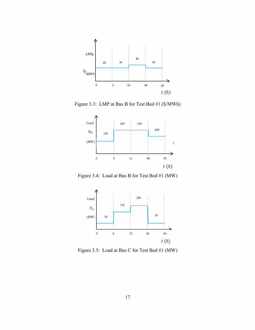
17

Figure 3.3: LMP at Bus B for Test Bed #1 ($/MWh)

Figure 3.4: Load at Bus B for Test Bed #1 (MW)

Figure 3.5: Load at Bus C for Test Bed #1 (MW)

18

Figure 3.6: Wind Generation at Bus B for Test Bed # 1 (MW)

Figure 3.7: Wind Generation at Bus C for Test Bed # 1 (MW)

3.3 Formulation of the Problem

The main objective is to maximize beneficial impacts of storage, mainly reflected as minimizing generation dispatch cost. A storage facility is considered to be present at Bus A in Figure 3.1. A QP based algorithm is carried out to optimize generation and storage scheduling with maximal use of renewable generation. For the tests reported, all the wind generation is used. The un-knowns, optimum generation schedule and storage (store/discharge) schedule are calculated, minimizing the purchase price of energy for one day. The information used and constraints con-sidered are:

Given Information

Loads

Wind power

LMPs at generation buses

Constraints

Line loads

Energy and power of storage

Conservation of power at each bus

Voltage phase angle at each bus

Bus A is assumed to be the reference bus. The voltage phase angle at each bus constrained to lie between -30o ≤ δ ≤ 30o. Three cases are studied calculating the economic dispatch of generation at bus A (PA) and bus B (PB) for minimum cost with:

19

No storage and no constraints line ratings.

Constraint on line ratings and one storage unit at bus A.

Constraint on line ratings and two storage units at bus A and B. All the three cases are studied for a one day time horizon broken into 4 intervals each have a span of 6 hours.

3.4 Study of Case 1 (base case)

In this case study, the system is initially assumed without energy storage and without constraints on line ratings are considered. After executing the economic dispatch considering the limits on generation, the output of generating units PA and PB computed is listed in Table 3.2. The mini-mum generation cost of the system without energy storage using QP in Matlab is 181,520 dollars per day. At interval 1 and 4, the load is being supplied by the cheap unit A. At intervals 2 and 3, the cheap unit B has to supply power.

Table 3.2: Case 1 Study Results, Test Bed #1

Interval (each Operational data 6 hours) 1 2 3 4

Generation (MW)

Bus A 130 0 0 195

Bus B 0 335 395 0

Line flows (MW)

Bus A to Bus B 88.33 -70 -97.5 140

Bus A to Bus C 41.67 70 97.5 55

Bus B to Bus C -1.67 70 97.5 -100

Voltage an-gle (radians)

Bus B -0.0088 0.007 0.0097 -0.014

Bus C -0.0083 -0.014 -0.0195 -0.011

3.5 Study of Case 2

In this case study, with the energy storage at bus A having rating of 20 MW and energy capacity of 120 MWh. Economic dispatch of generations PA and PB is calculated for minimum cost using

20

QP in Matlab with storage and considering the limits on generations and thermal ratings of the transmission lines. The dispatch results are shown in Table 3.3. At the first low-load hour, the storage is charged by 20 MW which is from the cheap unit A. At intervals 2 and 3, the output from the storage is discharged mitigating the congestion on the line from bus A to bus C. In addi-tion the output from the battery is replacing generation from expensive unit A. The total genera-tion dispatch cost is 179,380 dollars per day which is less than that in Case 1. This saving could be much higher in the large system.

From Case 2 it is observed, the energy is stored during the minimum cost of generation and dis-charged when the cost of generation is high. At the end of the day the storage element is com-pletely discharged. In other words, the battery (storage element) charges during the first interval and discharges during the second and third interval to minimize the cost of generation.



Generation (MW) Bus A 150 0 0 195

Bus B 0 330 380 0

Line flows (MW)

Bus A to Bus B 88.33 -65.83 -85 140

Bus A to Bus C 41.67 70.83 100 55

Bus B to Bus C -1.67 69.17 95 -100

Voltage angle (radians)

Bus B -0.0088 0.0066 0.0085 -0.014

Bus C -0.0083 -0.0142 -0.02 -0.011

Storage (MW) Bus A 20 -5 -15 0

3.6 Study of Case 3

In case 3 the economic dispatch is solved with limits on line ratings and two storage units at bus A and bus B having combined rating of 20 MW and energy capacity of 120 MWh (10 MW and

21

60 MWh each). The results are shown in Table 3.4. The cost of economic dispatch of generation per day calculated is $ 179,080.

Figure 3.8: Three Bus Test Bed: Test Bed # 1 with Two Storage Units



Generation (MW)

Bus A 150 0 0 195

Bus B 0 335 375 0

Line flows (MW)

Bus A to Bus B 96.67 -70 -89.7 140

Bus A to Bus C 43.33 70 99.17 55

Bus B to Bus C -3.33 70 95.83 -100

Voltage angle (radians)

Bus B -0.0097 0.0070 0.0089 -0.014

Bus C -0.0087 -0.014 -0.0198 -0.011

Storage (MW) Bus A 10 0 -10 0

Bus B 10 0 -10 0

22

Inference drawn from this case is that the spreading the storage unit reduces the generation pro-duction cost. This is because of line rating constraints limiting concentrated energy storage. At the first low-load hour, the storage at bus A and bus B is charged by 10 MW each which is from the cheap unit A. At interval 4, the output from the storage is discharged mitigating the conges-tion on the line. In addition the output from the battery is replacing generation from expensive unit A and B. The total generation dispatch cost is 179,080 dollars per day which is less than that in case 2.

3.7 Impact of Storage: Observations from Test Bed # 1

The implementation and use of renewable energy may not always be possible due to constraints of transmission and component ratings, when storage is added; these constraints are partially re-laxed, this can be observed from cases mentioned above.

High prices are one of the largest barriers facing renewables. During peak demand on the electric grid, electric companies pay more for electricity. Often additional power needs at this time are supplied by natural gas or oil, which has higher fuel costs. The opposite is true during times of low demand, when electricity costs are lower, during this time the energy can be stored and dis-charged when the demand and fuel cost is high thereby reducing the overall cost of generation per day; this can be observed from the above discussed cases 1, 2 and 3.

The grid needs a consistent, stable supply of energy that can be adjusted during times of peak demand. Black out occurs when supply does not keep up with demand. High demand on the power grid often requires power plants to be fired up to cover short-term electricity demand at a higher price. Large-scale of use of renewable energy will require that it can adapt to variable lev-els of demand on the power grid. Energy storage combined with these renewable energy re-sources may firm up the power output.

The cost of delivery and generation (fuel) can be minimized by increasing the capacity of storage elements and fuel cost can be further optimized by disbursing the storage unit across the power system. This concept is illustrated in Figure 3.9. Here, corresponding to the total power (MW, across two storage units), six hours of energy storage (MWh) is considered.

23

Figure 3.9: Fuel Cost Comparison with One and Two Storage Unit

Energy storage gives additional degrees of freedom in the optimal dispatch problem, thereby po-tentially allowing the additional use of renewable energy. The simple example of test bed #1 shown has wind penetration in the range of 5 % (Wind peak power / Peak demand power). Much more significant improvements in operating strategies occur at higher storage capacities. This is shown in the Table 3.5.

24

Table 3.5: Cost Comparison with One and Two Storage Units

Total Storage Capacity (MW)

Fuel cost per day to serve the load ($/day)

One storage unit Two storage unit

0 181,520 181,520

10 180,320 180,320

20 179,380 179,080

30 178,810 177,910

40 178,210 177,010

50 177,610 176,110

60 177,010 175,210

70 176,410 174,310

80 175,810 173,410

90 175,210 172,510

100 174,610 171,610

110 174,010 170,710

120 173,400 169,810

25

4 Illustrative Example using the State of Arizona as a Test Bed

4.1 Description of the Test Bed: State of Arizona

The previous chapter provided an introduction test system to demonstrate the idea of optimal scheduling of energy storage. This chapter looks at more realistic and well-studied example. In this section, the effect of energy storage on the minimization of the objective function using the State of Arizona as a test bed with different storage capacities and wind generation is studied. This benchmark system which represents a portion of the Western Electricity Coordinating Council (WECC) as of April 2009 does not include storage. Therefore, while the use of its net-work topology, generation bounds as well as transmission line ratings bounds, appropriate values for the storage parameters are added in the profile. The load, wind power and LMPs (assumed, at generation bus) at each bus are also given. The heavy summer case of 2009 is considered (actual load and generation data).

In the test case, an objective function is minimized. Again, this corresponds to minimum operat-ing cost. The constraints and formulation of the problem is the same as provided in the previous chapter. A QP based algorithm is carried out to optimize generation and storage scheduling with maximal use of renewable generation. The optimum generation schedule, storage (store / dis-charge) schedule, and line flows are control variables, and these quantities are calculated.

A one day time horizon broken into 3 intervals each having a span of 8 hours is studied. The ob-jective of the constrained economic dispatch is to schedule the generation outputs economically including storage over one day. The simplifications made are:

Reactive power flows are not modeled or considered

A simple linear relationship is assumed between bus voltage phase angle and line active power flows

Transmission line losses are neglected. The portion of the WECC under study is mainly the state of Arizona having the description pro-file indicated in Table 4.1.

Table 4.1: Description Profile: State of Arizona Power System

Number of buses nb 792 Number of generators 182

Number of lines nl 1079 Number of wind farms * 2 *Assumed

4.2 Case 4

Case 4 is a ‘base case’ study for this test bed. In case 4, no storage units are scheduled and two wind farms are located at Flagstaff and Springerville. Economic dispatch of generations is calcu-lated for the minimum cost using QP in the Matlab optimization toolbox. According to the con-straints considered in this work, only active power constraints are considered. Therefore, the re-

26

spective maximum and minimum operating long term thermal ratings of the transmission lines, generation limits and voltage phase angle limits at each bus is accommodated in the upper (UB) and lower bound (LB) of the program.

Table 4.2 shows the operational data for case 4. The cost of economic dispatch of generation per day calculated is 12.049 million dollars per day (M$/day).

Table 4.2: Case 4 Study Results, Arizona Test Bed

Wind Storage

P1 (MW) P2 (MW) P1 (MW) W1(MWh) P2 (MW) W2 (MWh)

400 300 0 0 0 0

4.3 Case 5 – Storage Added

In case 5, the wind power capacity and storage capacity is increased. The case is divided under low, medium and high depending on wind power penetration and storage capacity of the power system. Two wind farms are considered located at Flagstaff and Springerville along with two storage units both at Navajo. The storage units have two ratings, one relating to the power elec-tronic converters (this is the power rating of the unit), and the other as the ultimate energy stor-age capability (this is the energy rating, e.g., in MWh). For case 5, it is assumed that the power rating (MW) times 6 hours is the energy (MWh) rating. Table 4.3 tabulates the description of the wind power and storage as well as the solution cost. It is observed that with increasing energy storage, the operating cost reduces. Note that electrical energy is stored during times when generation cost is low and when production exceeds con-sumption. The stored energy is discharged during the period when the production cost from con-ventional generating plants is high.

27


Scenario

Operational data

Low 1

Medium 2

High 3

Win

d

P1 (MW) 400 600 800

P2 (MW) 300 500 600

Stor

age

P1 (MW) 50 100 300

P2 (MW) 50 150 250

W1 (MWh) 300 600 1800

W2 (MWh) 300 900 1500

Cos

t

QP (Million dollars / day) 11.772 11.453 11.066

4.4 Case 6 – Increase in the Number of Storage Units

In case 6, three scenarios are studied. The number of energy storage units is increased from 2 to 4 to 6. In each scenario, the total power and energy stored is the same, i.e. total power capacity = PST = 700 MW and total energy WST = 4200 MWh. These levels are shared among the storage units. The wind power is the same as assumed in case 4. Table 4.4 tabulates the number of stor-age units and economic dispatch cost in millions of dollars per day obtained using QP for the re-spective scenarios.

The results indicate that the cost of delivery and generation (fuel) can be minimized by increas-ing the capacity of storage elements. The fuel cost can be further optimized by selecting opti-mum locations for the two storage units.

28


Scenario Operational Data

1 2 3

Sto

rage

Number of Units 2 4 6

P (MW) each unit 350 175 116.67

W (MW) each unit 2100 1050 700

Cos

t

QP (M$/day) 11.616 11.563 11.484

4.5 Case 7 – Large Scale Implementation

This case resembles more of a practical scenario. In other words, a large number of wind ma-chines are accommodated. Note that the 2025 renewable portfolio standard for Arizona is 15%; a higher percentage of wind generation is accommodated in case 7. In case 7, 15% of the total load is derived from wind generation. Also, ten energy storage units are represented having a total capacity of 700 MW with 6 hours of energy storage (i.e., the total energy rating is 6 times 700 or 4200 MWh). Table 4.5 shows the system description.

Table 4.5: Case 7 System Description

Number of buses nb 792 Number of lines nl 1079

The wind availability considered throughout the day for case 7, and this is shown in Fig. 4.1. The wind turbines are assumed to generate power at name plate rated capacity. The cost of economic dispatch of generation computed is 10.863 million dollars per day (M$/day).

The inference made from this case is the optimal location of energy storage units is at the genera-tion buses. This observation is made for storage units such as batteries; however, obviously, the location of pumped-hydro storage is dictated by geography and topography. Storage units can be placed next to wind farms to produce a consistent flow of power. Locations like Bullhead City have a high potential of wind production [5]. Siting wind generation at such locations may be de-pendent on ratings of the adjacent transmission facilities. Storage unit placed at these locations can store excess wind energy and discharge during later periods. Therefore, use of storage can reduce the cost of upgrade of the electricity link and defer the expansion of the transmission net-work.

29

Figure 4.1: Wind Generation Patterns for Case 7, t is in hours

4.6 Calculation of Payback Period

The payback period in capital budgeting refers to the period of time required to return an invest-ment, to repay the sum of the original investment. An approximate payback period is calculated for the above discussed cases 5, 6 and 7. Mathematically, the length of time required to recover the cost of an investment is calculated as:

Cost of Project = Nyears * Annual Cash Inflows

There are two main problems with the payback period method:

It ignores any benefits that occur after the payback period and, therefore, does not meas-ure profitability.

It ignores the time value of money.

Annual cash inflows is the savings obtained from cases 5, 6, and 7 when compared with case 4. Following assumption is made: the energy storage system is a lead-acid battery and wind turbine is a doubly fed induction generator (DFIG), type 3 is assumed. The calculation is,

Cost of lead-acid battery, CB = 0.17 $/Wh.

Cost of wind turbine, CW = 1.2 to 2.6 million $/MW of name plate capacity.

30

Cost of electronics (converter), CE = $ 250 per kW.

Let, ND = Number of days for repay of the original investment. Then the value of ND is found for the several cases:

Case 5: The wind power capacity and storage capacity is increased. The case is divided under low, medium and high depending on wind power penetration and storage capacity of the power system. The case 5 test bed has two energy storage systems and two wind turbines with the elec-tronic converters.

Low case scenario: Total cost of battery storage is,

CBT = Number of units × Storage capacity (Wh) × Cost of lead acid battery ($/Wh)

= 2×300×106×0.17= $ 102 million.

Cost of electronics for the two storage units,

CET = 2×250×50000= $ 25 million.

Cost of wind turbines,

CWT = (400+300) ×1.2= $ 840 million.

Total initial investment is,

Ci = CBT + CET+ CWT= $ 967 million.

Saving’s with respect to case 4,

S= $ 0.277 million /day.

Thus, an approximate payback period is, SND = Ci

⇒ ND= Ci / S=3490.97 days = 9.56 years

Note: The above calculation does not take account of maintenance and battery replacement with inflation rate for the total system. By the same token, the approximate payback period in years for medium case and high case scenario is 7.52 years and 6.63 years respectively.

Case 6: The number of energy storage units is increased from 2 to 4 to 6. In each scenario, the total power and energy stored is kept the same, i.e. total power capacity = PST = 700 MW and total energy WST = 4200 MWh. The payback period for 2, 4 and 6 storage units is found to be 10.93 years, 9.74 years and 8.38 years.

Case 7: This case resembles more of a practical scenario. In other words, a large number of wind machines are accommodated. Here, 15% (4400 MW) of the total load is derived from wind gen-eration. Also, ten energy storage units are represented having a total capacity of 700 MW with 6

31

hours of energy storage (i.e., the total energy rating is 6 times 700 or 4200 MWh). The payback period is 14.25 years. Figure 4.2 represents the payback period of each case.

Figure 4.2: Payback Period for Cases 5, 6, 7

9.56

10.93

7.52

9.74

14.25

6.63

8.38

0

2

4

6

8

10

12

14

16

Case 5 Case 6 Case 7

Year

s pay

back

Case 5 increasing storage and wind. Case 6 spreading storage units

Case 7 state of Arizona

Low

Med

Hig

h

2 un

its

4 un

its

6 un

its

32

5 Conclusions and Future Work

5.1 Conclusions and Main Contributions

It has been shown in this report that energy storage devices not only facilitate the large scale in-tegration of renewable energy resources into the grid, but also assist in the economic dispatch of generation. In this research, an equivalent section of the WECC system, namely for Arizona, summer peak 2009 was considered. The following main conclusions can be made from the re-sults presented in the previous chapters:

In the base case (Case 4) without energy storage, the minimum generation dispatch cost of the system is 12.049 million dollars per day and the economic dispatch with the energy storage in system for a comparable case.

(Case 5) the total generation dispatch cost is 11.772 million dollars per day. The savings increases with an increase in storage capacity. Quantitatively, for the cited case an in-crease in savings of 0.277 to 0.596 million dollars per day is attained for addition of 900 MWh.

The test bed state of Arizona with accommodation of 15% (4400 MW) of the total load being served from wind production and 4200 MWh of energy storage the total generation dispatch cost is 10.863 million dollars per day. This figure is observed for the summer 2009 peak period.

Large scale energy storage can be used to mitigate the overloading of the transmission lines at places where the wind energy potential is high and connection to the grid is ex-pected. For example, in Case 7, wind generation sited at Bullhead City AZ was studied and energy storage at this site is allowed. The addition of 250 MW of wind despite the 140 MW adjacent existing transmission. In this example energy storage is rated at 720 MWh, with a converter rating of 120 MW.

Defer the upgrade of the transmission systems when renewable resources are added. This results as the usage of energy storage can reduce the power transfer through adjacent lines during peak load periods. Also, the use of storage can decrease the congestion cost as energy storage systems can shift the load from the peak to off-peak load periods. This advantage was illustrated in Case 7 in which up to 116 MW in the period 0800 to 1600 hours is shifted to the period 1600 to 0000 hours. This 116 MW shift was in a line of rat-ing of 398 MVA.

Disbursing the storage units across the state of Arizona reduces the generation production cost. This is the case because of line rating constraints limiting concentrated energy stor-age. Case 6 illustrates this point through the comparison of the utilization of 2, 4, and 6 storage units.

33

Secondary contributions are:

Quadratic programming has been illustrated as an optimization method for scheduling energy storage.

Examples have been shown with an actual power system for the state of Arizona.

Sample code in Matlab has been developed (see Appendix A).

5.2 Future Work

In the present work, the objective cost function is based on the power generated from power plants. The thesis mainly focuses on economic dispatch using the state of Arizona as a test bed. This work can be extended by modeling the system external to Arizona and implementing the following:

Address the dimensionality problem.

Include the impact of energy storage on the reduction of spinning reserve.

Model the transmission and storage devices losses occurring in the power system.

Model the storage technologies characteristics to better represent each of them.

Include a dynamic response study to study the system stability. Also, check voltage sta-bility in the steady state and in the dynamic case.

Study the power quality issues in the grid due to the appearance of high levels of DC/AC and AC/DC conversion.

Perform reactive power studies.

.

34

References

1. Global Wind Energy Council, no title, [online], Available: http://www.gwec.net/ 2. B. C. Ummels., M. Gibescu, E. Pelgrum, L. W. Kling., A. J. Brand. Impacts of wind

power on thermal generation unit commitment and dispatch. IEEE Trans. Energy Con-vers., 2007, vol. 22, pp. 44-51, March 2007.

3. U.S. Energy Information Administration. Renewables and alternative fuels. http://www.eia.gov/renewable/data.cfm#wind, August 2011.

4. Black; and Veatch. Twenty percent wind energy penetration in the United States: A tech-nical analysis of the energy resource. Walnut Creek, CA, October 2007.

5. National Renewable Energy Laboratory. Wind resource potential-2010. http://www.windpoweringamerica.gov/wind_maps.asp, September 2011.

6. Power of Wind, American wind energy brochure, no title, [online], Available: http://www.awea.org/learnabout/publications/upload/AmericanWindpowerBrochure.pdf .

7. U.S. Department of Energy. 20% wind energy by 2030. http://www.nrel.gov/docs/fy08osti/41869.pdf, July 2008.

8. Kristina Hamachi LaCommare and Joseph H. Eto. Cost of power interruptions to elec-tricity consumers in United States (U.S.). Ernest Orlando Lawrence Berkeley National Laboratory, February 2006.

9. Wiser, R.; and M. Bolinger. Annual report on U.S. wind power installation, cost, and performance trends: 2007. [online], Available: http://www.nrel.gov/docs/fy08osti/43025.pdf, May 2008.

10. Sandia National Laboratories. Electric power industry needs for grid-scale storage appli-cations. [online], Available: http://energy.tms.org/docs/pdfs/Electric_Power_Industry_Needs_2010.pdf

11. U.S. Energy Information Administration. Wind generation. (September 2011). Available: http://www.eia.gov/cneaf/solar.renewables/page/wind/wind.html.

12. Arizona Public Service Co. Challenges of Electricity Storage Technologies. A report from the APS panel on public affairs Committee on Energy and Environment, May 2007.

13. Schoenung, S.; and C. Burns. Utility energy storage applications studies. IEEE Trans. Energy Conversion, vol. 11, pp. 658-665, Mar. 1996.

14. Yeleti, S.; and Yong Fu. Impacts of energy storage on the future power system. North American Power Symposium (NAPS) 2010, pp. 1-7, 26-28 Sept. 2010.

15. Spahic, E.; G. Balzer, B. Hellmich, and W. Munch. Wind energy storage – possibilities. IEEE Lausanne Power Tech 2007, pp. 615-620, 1-5 July 2007.

16. Ibrahim, H.; A. Ilinca, and J. Perron. Comparison and analysis of different energy stor-age techniques based on their performance index. IEEE Electrical Power Conference, Canada, 2007, pp. 393-398.

17. Barote, L.; and C. Marinescu. Storage analysis for stand-alone wind energy applications. 12th International Conference on Optimization of Electrical and Electronic Equipment (OPTIM), pp. 1180-1185, 20-22 May 2010.

18. Anderson, M. D.; and D. S. Carr. Battery energy storage technologies. Proceedings of the IEEE, vol. 81, no. 3, pp. 475-49, Mar. 1993.

http://www.gwec.net/

http://www.eia.gov/renewable/data.cfm#wind

http://www.windpoweringamerica.gov/wind_maps.asp

http://www.awea.org/learnabout/publications/upload/AmericanWindpowerBrochure.pdf

http://www.nrel.gov/docs/fy08osti/41869.pdf

http://www.nrel.gov/docs/fy08osti/43025.pdf

http://energy.tms.org/docs/pdfs/Electric_Power_Industry_Needs_2010.pdf

http://www.eia.gov/cneaf/solar.renewables/page/wind/wind.html

35

19. Lumb, D.; and N. T. Hawkins. Provision of power reserve from pumped storage hydro plant. IEE Colloquium on Economic Provision of a Frequency Responsive Power Re-serve Service, pp.3/1-3/4, 5 Feb. 1998.

20. Farahani, M. E. S.; and N. Saeidi. Case study of design and implementation of a thermal energy storage system. IEEE International Power and Energy Conference 2006, pp. 6-11, 28-29 Nov. 2006.

21. Sioshansi, R.; and P. Denholm. The value of concentrating solar power and thermal en-ergy storage. IEEE Transactions on Sustainable Energy, vol. 1, no. 3, pp. 173-183, Oct. 2010.

22. Monkhouse, S. E.; and L. C. Grant. The heating of buildings electrically by means of thermal storage. Journal of the Institution of Electrical Engineers, vol. 68, no. 402, pp. 657-665, June 1930.

23. Hirscher, Michael; and Katsuhiko Hirose. Handbook of hydrogen storage: new materials for future energy storage. Wiley Publications, New Jersey, ISBN 978-3-527-3273-2, May 2010.

24. U.S. Department of Energy. Hydrogen program. Available: http://www.hydrogen.energy.gov/, July 2010.

25. Boyes, J. D.; and N. H. Clark. Technologies for energy storage: flywheels and super con-ducting magnetic energy storage. IEEE Power Engineering Society Summer Meeting 2000, vol. 3, pp. 1548-1550, May 2000.

26. Schainker, R. B. Executive overview: energy storage options for a sustainable energy future. IEEE Power Engineering Society General Meeting, 2004. (2), pp. 2309-2314.

27. U.S. Department of Energy. Economic dispatch of electric generation capacity: a report to congress and the states pursuant to sections 1234 and 1832 of the energy policy act of 2005. Available: http://www.hydrogen.energy.gov/, July 2010.

28. Happ, H. H. Optimal power dispatch-a comprehensive survey. IEEE Transactions on Power Apparatus and Systems, vol.96, pp. 841-854, May/June 1977.

29. IEEE Working Group. Description and bibliography of major economy-security func-tions. Part II-bibliography (1959-1972). IEEE Transactions on Power Apparatus and Systems, vol.100, pp. 215-223, Jan. 1981.

30. IEEE Working Group. Description and bibliography of major economy-security func-tions. Part III-bibliography (1973-1979). IEEE Transactions on Power Apparatus and Systems, vol.100, pp. 224-235, Jan. 1981.

31. Wood, J.; and B. F. Wollenberg. Power Generation, Operation and Control. John Wiley & Sons, New York, 1984.

32. Li, Chao-An; Raymond B. Johnson, and Alva J. Svoboda. A new unit commitment meth-od. IEEE Transactions on Power Systems, vol. 12, no. 1, pp. 113-119, Feb. 1997.

33. Zhu, Jizhong. Optimization of power system operation. John Wiley & Sons, New Jersey, 2009.

34. Srinivasan, D.; and A. Tettamanzi. A heuristic-guided evolutionary approach to multi-objective generation scheduling. IEEE Proceedings Generation, Transmission, and Dis-tribution, vol. 143, no. 6, pp. 553-559, Nov. 1996.

35. Anonymous. Optimization Toolbox for use with Matlab. Mathworks.

http://www.hydrogen.energy.gov/

http://www.hydrogen.energy.gov/

36

36. Laithwaite, E. R.; and L. L. Freris. Electrical Energy: its generation, transmission and use, McGraw-Hill Book Company (U,K,), 1980.

37. Bellman, R. The theory of dynamic programming. RAND Corporation, Proc. National Academy of Sciences, pp. 503-715, 1952.

37

APPENDIX A MATLAB CODE

A.1 Matlab Code Used in this Project

A sampling of the key Matlab scripts used in this work are provided in this appendix.

clear; clc; tic; %% Main system data nb=792; % Number of bus nl=1079;% Number of lines h=3; % Intervals of each 24/h hours ng=nb; % Storage and generation assumed at all buses. Zero storage and nst=nb; % generation is accommodated in lower and upper bounds Base=100; %% Read data B = xlsread('AZ.xlsx','Line Records','b1:b10000'); % From bus D = xlsread('AZ.xlsx','Line Records','d1:d10000'); % To bus J = xlsread('AZ.xlsx','Line Records','k1:k10000'); % Reactance U=xlsread('AZ.xlsx','Bus Records','n2:n10000'); % Load V=xlsread('AZ.xlsx','Bus Records','o2:o10000'); % Wind Y=xlsread('AZ.xlsx','Line Records','m1:m10000'); % Line ratings S=xlsread('AZ.xlsx','Storage','q1:q10000'); % Energy stored P=xlsread('AZ.xlsx','Storage','p1:p10000'); % Power Stored G=xlsread('AZ.xlsx','Storage','r2:r10000'); % Generation ratings %% Cost function to be minimized c=zeros(1,ng*h+nl*h+nst*h+(nb-1)*h); H=zeros(ng*h+nl*h+nst*h+(nb-1)*h,ng*h+nl*h+nst*h+(nb-1)*h); Q=xlsread('AZ.xlsx','Storage','s2:s10000'); C=xlsread('AZ.xlsx','Bus Records','t2:t10000'); n=0;k=0; for ro=1:h:ng*h; q=Q(ro+k-n)*Base; for added=1:h; H(ro+added-1,ro+added-1)=2*q; end k=k+1; n=n+h; end f=C*Base;

38

for i=ng*h+1:ng*h+nl*h+nst*h+(nb-1)*h; f(i,1)=0; end %% Formation of bus dictionary busdict=zeros(nb,1); busdict(1)=10435; % running=1; for iline=1:nl; ifrom = B(iline); ito = D(iline); xline=J(iline); ifound=0; for i=1:running; if busdict(i)==ifrom; ifound=i; ifromn=i; end; end; if ifound == 0; running=running+1; busdict(running)=ifrom; ifromn=running; end; ifound=0; for i=1:running; if busdict(i)==ito; ifound=i; iton=i; end; end; if ifound == 0 running = running+1; busdict(running)=ito; iton=running; end; end; busdict1=sort(busdict); %% Formation of equality constraints % Formation of Aeq aeq=sparse(nb*h+nl*h+1,(3*nb-1+nl)*h);

39

inb=sparse(eye(nb*h,nb*h)); aeq(1:nb*h,1:nb*h)=inb; % Generation at buses aeq(1:nb*h,(nb)*h+1:(nb+nst)*h)=-inb; % Storage at buses % Stored energy at end of day should be zero aeq(nb*h+nl*h+1,(nb)*h+1:(nb+nst)*h)=24/h; % Line injection power inh=sparse(eye(h,h)); for k=1:nl; stb=B(k); stbb=0; for look=1:nb; if busdict1(look)==stb; stbb=look; end; end; endb=D(k); endbb=0; for look=1:nb; if busdict1(look)==endb; endbb=look; end; end; aeq(h*(stbb-1)+1:h*(stbb-1)+h,nb*h+nst*h+1+h*(k-1):... nb*h+nst*h+h*(k-1)+h)=-inh; aeq(h*(endbb-1)+1:h*(endbb-1)+h,nb*h+nst*h+1+h*(k-1):... nb*h+nst*h+h*(k-1)+h)=inh; end; for k=1:nl; x=J(k); stb=B(k); stbb=0; for look=1:nb; if busdict1(look)==stb; stbb=look; end; end; endb=D(k); endbb=0; for look=1:nb; if busdict1(look)==endb; endbb=look; end

40

end if stbb~=1; aeq(nb*h+1+(k-1)*h:nb*h+(k-1)*h+h,(2*nb*h+nl*h)+1+(stbb-2)*h:... (2*nb*h+nl*h)+(stbb-2)*h+h)=-1/x*inh; end if endbb~=1; aeq(nb*h+1+(k-1)*h:nb*h+(k-1)*h+h,(2*nb*h+nl*h)+1+(endbb-2)*h:.... (2*nb*h+nl*h)+(endbb-2)*h+h)=1/x*inh; end end inl=sparse(eye(nl*h,nl*h)); aeq(nb*h+1:(nb+nl)*h,nb*h+nst*h+1:(nb+nst+nl)*h)=inl;% Power Flow vs. delta %Formation of beq beq=zeros(nb*h+nl*h+1,1); for k=1:nb*h load=U(k)/Base; wind=V(k)/Base; beq(k,1)=load-wind; end %% Formation of inequality constraints % Formation of A a=sparse(nl*h*2+nst*h,ng*h+nl*h+nst*h+(nb-1)*h); a(1:nl*h,(ng+nst)*h+1:(ng+nst+nl)*h)=inl; % Upper line rating a(nl*h+1:(nl+nl)*h,(ng+nst)*h+1:(ng+nst+nl)*h)=-inl;% Lower line rating % Maximum energy stored n=0;m=0; for i=1:nst; a(2*nl*h+1+m:2*nl*h+(h-1)+m,ng*h+1+n:ng*h+h-1+n)=... sparse(tril(ones(h-1,h-1)))*24/h; k=a(2*nl*h+1+m:2*nl*h+(h-1)+m,ng*h+1+n:ng*h+h-1+n); if h==3; a(2*nl*h+h+m:2*nl*h+h+m,ng*h+1+n:ng*h+h-1+n)=-k(2:h-1,1:h-1); j=m; else a(2*nl*h+h+m:2*nl*h+h+h-3+m,ng*h+1+n:ng*h+h-1+n)=-k(2:h-1,1:h-1); j=m; end n=n+h;m=2*h+m-3; end

41

% Maximum stored power inb=sparse(eye(nb*h,nb*h)); a(2*nl*h+2*h-2+j:2*nl*h+2*h-3+j+nst*h,(nb)*h+1:(nb+nst)*h)=inb; % Formation of b b=zeros(nl*h*2+nst*h,1); k=0; for j=1:nl; kline=Y(j)/Base; b(1+k:h+k,1)=kline; % Line ratings k=k+h; end k=0; for j=1:nl; kline=Y(j)/Base; b(nl*h+1+k:nl*h+h+k,1)=kline; % Line ratings k=k+h; end m=0;j=0;n=0; for i=1:nst; s=S(i)/Base; % Energy stored b(2*nl*h+1+m:2*nl*h+h-1+m,1)=ones(h-1,1)*s; if h==3; b(2*nl*h+h+m:2*nl*h+h+m,1)=ones(h-2,1)*0; j=m; else b(2*nl*h+h+m:2*nl*h+h+h-3+m,1)=ones(h-2,1)*0; j=m; end m=2*h+m-3; end k=0; for i=1:nst; p=P(i)/Base; % Maximum Power stored b(2*nl*h+2*h-2+j+k:2*nl*h+3*h-3+j+k,1)=ones(h,1)*p; k=k+h; end %% Construct lb and ub vectors lb=zeros((3*nb-1+nl)*h,1); k=0;n=0; for ro=nb*h+1:h:2*nb*h; lb(ro)=0; es=ro-nb*h-h*k+n;

42

rate=P(es)/Base; for added=1:h-1; lb(ro+added)=-rate; end; k=k+1;n=n+1; end; n=0;k=0; for ro = 2*nb*h+1:h:2*nb*h+nl*h; y=-Y(ro-2*nb*h-h*k+n)/Base; for added=1:h; lb(ro+added-1)=y; end k=k+1;n=n+1; end lb(2*nb*h+nl*h+1:(3*nb-1+nl)*h,1)=-pi/6; % voltage angle within 30 degree ub=-lb; n=0;k=0; for ro=1:h:nb*h; g=G(ro+k-n)/Base; for added=1:h; ub(ro+added-1)=g; end k=k+1;n=n+h; end k=0;n=0; for ro=nb*h+1:h:2*nb*h; ub(ro+h-1)=0; es=ro-nb*h-h*k+n; %es=((ro-h*(n+2)-1)/h+k); rate=P(es)/Base; for added=1:h-1; ub(ro+added-1)=rate; end; k=k+1;n=n+1; end; options=optimset('Algorithm','interior-point-convex'); [X,fval]=quadprog(H,f,a,b,aeq,beq,lb,ub,[],options); %Aeq=full(aeq); toc;

43

APPENDIX B The Quadratic Programming Algorithm

B.1 Quadratic Programming

QP model of economic dispatch Let the initial operating point of generator i be P0

geni. Expanding the nonlinear objective function using Taylor series 33,

fi(Pgeni) = fi(P0geni) +

geniPgeni

genii

dPPdf

0

)(ΔPgeni +

geniPgeni

genii

dPPdf

0

2

2 )(21

ΔP2geni + …

= a ΔP2

geni + b ΔPgeni + c

fi(ΔPgeni) = a ΔP2geni + b ΔPgeni

where

a = geniP

geni

genii

dPPdf

0

2

' )(21

b = geniP

geni

genii

dPPdf

0

2

)(

c = fi(P0

geni)

are constant and

ΔPgeni = Pgeni - P0geni

Power balance equation Since loads are constant for the given time and using Kirchhoff’s law, the following expression of power balance equation obtained,

∑Pgeni=∑PLk

Linearization of branch flow constraints The real power flow equation of a branch is,

Pij = Vi2gij – ViVj (-gijcosθij + bijsinθij)

where, Pij The sending end real power on transmission branch ij Vi The node voltage magnitude of bus i θij The difference of bus voltage angles between the sending and receiving end of the line ij gij The conductance of transmission branch ij bij The susceptance of transmission branch ij.

44

Linearizing the power flow equation and considering a high voltage network, the value of θij is very small. In addition, assuming the magnitudes of all the bus voltages equal to 1.0 p.u. and the reactance of the line is much bigger than resistance of the line, then Δ Pij = - bijΔθij =

ij

ji

X Generator and storage power constraints

0≤ Pgeni≤ Pgeni max iϵ NG Psq min ≤ Ps ≤ Psq max q ϵ ns

The QP algorithm Quadratic programming is the problem of finding a vector X that minimizes a quadratic function, subject to linear constraints:

Minimize XCQXX TT (B.1) Such that eqeq bXA (B.2)

bAX (B.3) lb ≤ X ≤ ub

(B.4)

where C is an n-dimensional row vector of cost of generation, Q is an (n×n) symmetric matrix describing the coefficients of the quadratic terms, the decision variables are denoted by the n-dimensional column vector X, and the constraints are defined by an (m×n) A, Aeq matrix and an m-dimensional column vector b, beq of right-hand-side coefficients. When the objective function f(X) is convex for all feasible points, the problem has a unique local minimum, which is also the global minimum.

The equation (b.3) can be expressed as 33, g(X) = (AX-b)≤ 0 (B.5) The lagrangian for (B.1) and (B.5) is,

L(X, μ) = CX + XTQX + μg(X) where μ is an m-dimensional row vector. According to optimization theory, the Kuhn-Tucker (KT) conditions for a local minimum are given as,

45

02

,...,1,0

AQXC

njdXdL

T

j

(B6)

0

,...,1,0

BAX

njddL

i

(B.7)

0)2(

,...,1,0

TTT

jj

AQXCX

njdXdLX

(B.8)

0)(

,...,1,0)(

BAXmiXg ij

(B.9)

00X

(B.10)

Introduction of nonnegative variables y to the inequalities in equation (B.6) and nonnegative var-iables v to the inequalities in equation (B.7), to obtain,

CT + 2QX + ATμT – y =0 (B.11)

AX – B +v = 0 (B.12)

Then, the KT conditions are written as,

2QX +ATμT – y = -CT (B.13) AX + v = B (B.14)

X≥0, μ≥0, y≥0, v≥0 (B.15) yTX = 0, μv=0 (B.16)

The KT conditions in equations (B.13) to (B.16) have a linear form with the variables X, μ, y, and v. An interior point convex algorithm can be used to solve the equations (B.13) to (B.16). The interior point convex algorithm performs the following steps 35:

Presolve/Postsolve Generate initial point Predictor-corrector Multiple corrections

tools and techniques for considering transmission … and techniques for considering transmission...

Documents