Threshold cointegration: overview and

implementation in R

Matthieu Stigler

Matthieu.Stigler at gmail.com

January 10, 2010

(Revision 5: April 2013)

Abstract

Purpose of this paper is twofold. It is first to offer a rough overview

on the field of threshold cointegration, from the seminal paper of Balke

and Fomby (1997) to the recent developments. Simultaneously, it is to

describe the implementation of the main functionalities for the modeling

in the open-source package tsDyn. It provides hence a unique way to get

an introduction on the threshold cointegration field allowing in the same

time to conduct its own analysis.

Introduced by Engle and Granger (1987), the concept of cointegra-

tion became a indispensable step in the analysis of non stationary time

series. The underlying idea is that even if two variables (or more) are

non-stationary, there can exist a combination of them which is station-

ary. This definition leads to interesting interpretations as the variables

can then be interpreted to have a stable relationship (a long-run equilib-

rium), can be represented in an vector error-correction model, and share

a common stochastic trend.

However, implicit in the definition is the idea that every small de-

viation from the long-run equilibrium will lead instantaneously to error

correction mechanisms. Threshold cointegration extends the linear coin-

tegration case by allowing the adjustment to occur only after the de-

viation exceed some critical threshold, thus taking into account possibly

transaction costs or stickiness of the prices. Furthermore, it allows to cap-

ture asymmetries in the adjustment, where positive or negative deviations

won’t be corrected in the same manner.

1

Contents

1 Introduction: linear cointegration 3

2 The extension to threshold cointegration 5

3 The TAR model: probabilistic structure 8

4 Estimation and inference 10

4.1 Estimation and inference in the long-run relationship representation 10

4.1.1 The one threshold case . . . . . . . . . . . . . . . . . . . . 10

4.1.2 The two threshold case . . . . . . . . . . . . . . . . . . . 15

4.1.3 Distribution of the estimator . . . . . . . . . . . . . . . . 17

4.2 Estimation and inference in the TVECM representation . . . . . 20

5 Testing 23

5.1 The problem of the unidentified parameter . . . . . . . . . . . . . 24

5.2 Cointegration vs. threshold cointegration tests . . . . . . . . . . 25

5.2.1 Test based on the long-run relationship . . . . . . . . . . 25

5.2.2 Test based on the TVECM representation . . . . . . . . . 28

5.3 No cointegration vs. threshold cointegration tests . . . . . . . . . 28

5.3.1 Tests based on the long-run relationship . . . . . . . . . . 29

5.3.2 Unknown cointegrating values . . . . . . . . . . . . . . . . 32

5.3.3 Test based on the TVECM representation . . . . . . . . . 32

5.4 Conclusion for the test . . . . . . . . . . . . . . . . . . . . . . . . 33

6 Interpretation 33

6.1 Types of adjustment . . . . . . . . . . . . . . . . . . . . . . . . . 34

6.2 Non linear impulse response functions . . . . . . . . . . . . . . . 36

7 Running the functions on parallel CPUs 36

8 Conclusion 37

References 39

2

1 Introduction: linear cointegration

On stationarity When dealing with time series, a main concern for statistical

analysis is stationarity, the usual inference being based on that assumption. In

its weak version, stationarity is defined as the finiteness and time-invariance of

the expectation, variance and auto-covariance of a series. However, there are

considerable theoretical (Samuelson, 1965) and empirical (Nelson and Plosser,

1982) arguments in favor of non-stationarity of economic series, especially for

the difference-stationary type. A difference-stationary (or integrated) series is

defined as a series that is non-stationary, but whose difference is stationary, as

the random walk is. Great care should be taken when analyzing such series as

they follow a different asymptotic behavior and particularly, regression among

integrated series leads to a so-called spurious regression, i.e. inflation of re-

gression indicators (t-tests, R2) which lead to the false conclusion of statistical

dependence between the series (Granger and Newbold 1974, Philipps 1986). An

obvious remedy is to use differenced series, for which usual asymptotics apply.

This approach has become the standard in the VAR framework popularized by

Sims (1980).

Cointegration Granger introduced in 1982 the concept of cointegration, which

means integrated series for which a linear combination exists that is stationary.

This can be interpreted economically as the presence of a long-run equilibrium,

the relationship between the variables being stable. The concept gained a signif-

icant interest with the so-called Granger representation theorem, which states

that cointegrated variables have a vector error correction model (VECM) rep-

resentation, that can be seen as a VAR model including a variable representing

the deviations from the long-run equilibrium. Equation1 shows a VECM for

two variables including a constant, the error-correction term and a lag.

[∆Xt

∆Yt

]=

[c1

c2

]+

[a1

a2

]ECT−1+

[b11 b12

b21 b22

][∆Xt−1

∆Xt−1

]+

[εXt

εYt

]ECT−1 = (1,−β)

[Xt−1

Yt−1

](1)

This VECM representation is particularly interesting as it allows to esti-

mate how the variables adjust deviations towards the long-run equilibrium, to

test for Granger-causality as well as to determine the impacts of shocks to the

variables using impulse response functions. In a system with more than k > 2

3

variables, there may exist k − 1 cointegrating relationships, hence the vector A

of adjustment speed parameters (also called loading matrix) and the vector B

of cointegrating values become matrices1. The matrix of their product, corre-

sponding to the parameters of the lagged vector, is singular with rank equal to

the number of cointegrating relationships.

Two methods captured the main attention and are of popular use now. The

first one was advocated by Engle and Granger (hereafter E-G), who propose a

two-steps approach, estimating the cointegrating values in the long-run represen-

tation and then plugging those estimates one the VECM representation2. The

related testing procedure taking absence of cointegration as a null hypothesis

consists in determining whether the residuals from the first step are stationary

or not. Rejection of the stationarity is then interpreted as the rejection of the

null hypothesis of cointegration. When the cointegrating vector is known, usual

unit root tests can be applied, whereas in case it is unknown, different critical

values need to be used. Philipps and Ouliaris (1990) developed a test that is

invariant to the normalization available in the software R in package urca (Pfaff

2008a).

Estimation and testing A major drawback of the E-G approach is that

is allows to estimate and test only for one cointegrating relationship. When

the cointegrating vectors are known, estimation of multiple cointegration rela-

tionship is trivial as the estimation is simply OLS regression for the VECM

and testing can be done using classical Wald tests (Horvath and Watson 1995).

When these vectors are unknown, the reduced-rank approach adopted by Jo-

hansen (1998, 1995) is able to estimate the potential cointegrating vectors and

to test for their significance, allowing to determine the number of cointegration

relationships. This is available in R with the ca.jo() function from package vars

(Pfaff 2008b).

1of dimension r×k, with r the number of cointegrating values and k the number of variables2This two-step approach has been justified afterwards by the fact that the estimator in the

first step is super-consistent, i.e. converging to its true value at rate n instead of usual rate√n (Stock, 1987)

4

2 The extension to threshold cointegration

Balke and Fomby (1997) note that in the concept of cointegration there is the

implicit assumption that the adjustment of the deviations towards the long-run

equilibrium is made instantaneously at each period. There are nevertheless se-

rious arguments in economic theory to invalidate this assumption of linearity.

Among them, the presence of transaction costs is maybe the most noteworthy, as

it implies that adjustment will occur only once deviations are higher than the

transactions costs, and hence adjustment should not happen instantaneously

and at each time. Financial theory predicts that even in highly liquid mar-

kets a so-called band of no arbitrage may exist where deviations are too small

for the arbitrage to be profitable. In the domain of macroeconomics, policies

are often organized around targets, where intervention is activated only once

the deviations from the target are significant, the most famous example being

the monetary policy management during the Bretton Woods agreement where

central banks pegged their exchange rate and allowed a +/- 1 % band.

A second range of arguments that were raised in favour of nonlinear adjust-

ment concerns the assumption of symmetry. In the linear cointegration context,

increases or decreases of the deviations are deemed to be corrected in the same

way. Again, several theoretical arguments may contest this assumption, such as

the presence of menu costs ( Levy, Bergen, Dutta, and Venable, 1997, Dutta,

Bergen, Levy, and Venable, 1999), market power (Damania and Yang, 1998,

Ward, 1982) or simply small country vs rest of the world effects.

Balke and Fomby (1997) introduced the concept of threshold cointegration,

which allows to take into consideration the two main criticisms (though BF were

concerned only with the first one) raised against linear cointegration. In their

framework, the adjustment does not need to occur instantaneously but only

once the deviations exceed some critical threshold, allowing thus the presence

of an inaction or no-arbitrage band. They base their adjustment process on

the self-exciting threshold autoregressive model (SETAR3) introduced by Chan

(1983) and discussed extensively in Tong (1990). In the SETAR model, the

autoregressive coefficients take different values depending on whether the pre-

vious value is above or under a certain threshold value, thus exhibiting regime

switching dynamics. Hence, the linear adjustment process:

3But they call this model TAR, which is a more general form presented later.

5

εt = ρεt−1 + ut (2)

is extended as:

εt =

ρLεt−1 + ut if εt−1 ≤ θLρMεt−1 + ut if θL ≤ εt−1 ≤ θHρHεt−1 + ut if θH ≤ εt−1

(3)

This is actually a piecewise linear model where three different AR(1) pro-

cesses are estimated depending on the state of the variable at time t − 1. Au-

toregressive parameters are denoted with subscript L, M and H standing for

Low, Middle and High regime, and they differ whether the variable was below

the lower threshold θL, between the lower θL and upper θH threshold, or above

the higher θH . This leads to some further remarks:

� The threshold effect is present when ρH 6= ρMand ρL 6= ρM and as long

as 0 < P (ε < θb) < 1 where b = L or H

� The SETAR model nest the AR when ρH = ρM = ρL.

� The model can easily by extended by adding lags in each regime, as well

as intercepts.

� Several restricted models have been proposed, the main restriction being

that the outer regimes are symmetric (θL = θM along with ρH = ρL).

While the work of Balke and Fomby (1997) focused on the long-run relationship

representation, extension to a threshold VECM (TVECM) has been made by

several authors, the threshold effect being applied the anticipation by the agents

of interventionary policy only to the error-correction term (Granger and Lee

1989, Seo 2006) or to the lags and the intercept as well (Hansen and Seo 2002,

Lo and Zivot 2001 ).

[∆Xt

∆Yt

]=

[cX

cY

]+

[aXL

aY L

]ECTL,t−1[

aXM

aYM

]ECTM,t−1[

aXH

aY H

]ECTH,t−1

+

[b11 b12

b21 b22

][∆Xt−1

∆Yt−1

]+

[εXt

εYt

](4)

6

In this model, the error-correction term is split into three regimes, lower (L),

middle (M) and high (H) depending on whether it is below, between or above

the two thresholds θL and θH , as in 3.

Note that speaking of threshold cointegration in the case of the TVECM was

rather a conjecture as no formal representation theorem had been demonstrated

in the threshold case. Nevertheless, the intuition of these authors was justified

as Krishnakumar and Netto (2009) derived recently such a theorem, under the

assumption that the loading matrix (the matrix of coefficients a in 4) is diagonal.

An interesting conclusion of their theorem is that the threshold effect is present

on the lags also only if the residuals from the LR follow a multivariate SETAR

process with one lag in each regime. When the residuals follow a multivariate

SETAR process with p >1 lags, the lags in the TVECM do also have regime-

specific components.

Several other model specifications have been used in the literature. Gonzalo

and Pittarakis(2006a) and Krischnakumar and Netto (2009) use as transition

variable not the deviations itself, but an external variable (that is, a TAR model,

as we will see later). This has important implications as the stationarity con-

ditions are different, estimation is much easier, and testing is more restrictive4.

In that sense, it should be clearly differentiated from threshold cointegration as

introduced by BF and I will denote it by cointegration with threshold effects.

In my opinion, this approach is less attractive as it lets unanswered the question

why an influencing variable is not included in the VECM.

All previous studies were based on the definition of threshold cointegration as

a case where the variables are“linear”and the combination is linear, whereas the

adjustment process exhibits threshold effects. Gonzalo and Pittarakis (2006b)

take an opposite direction where the cointegrating relationship exhibits thresh-

old effects whereas the adjustment is linear5. That is, yt is I(1) and xt follows a

SETAR process, but there exists a linear combination of them which is station-

ary. Note that in that case, the notion of integratedness is undefined and there

is no corresponding VECM representation (Gonzalo and Pittarakis 2006a).

Empirical applications Since the seminal work of Balke and Fomby, thresh-

old cointegration has become widely applied in various contexts. The law of

4Current tests work only with a stationary external variable.5For an analogous case in the structural break literature, see Gregory and Hansen (1996)

7

one price (LOP) and the associated purchasing power parity (PPP) hypothe-

sis represent maybe the field where the greatest number of studies has been

conducted (see for a review on LOP Lo and Zivot, for the PPP, Gouveia and

Rodrigues 2004, Heimonen 2006, Bec et al. 2004). Numerous studies on price

transmission of agricultural products or other commodities (principally oil) use

the threshold cointegration framework. In the field of the term interest theory,

threshold cointegration methods have been developed and applied by Enders

and Granger (1998), Enders and Siklos (2001), Bec et al. (2008), Krishnakumar

and Netto (2009). Other fields include the Fisher effect (Million 2004), finan-

cial integration based on comparing local and the US stock markets (Jawadi

et al. 2009), exchange rate pass-through (Al-Abri and Goodwin 2009). To

my knowledge, however, the use of threshold cointegration remained within the

economical literature and no study has been done on other domains.

3 The TAR model: probabilistic structure

The Balke and Fomby approach was based on the use of the SETAR model de-

veloped by Chan and Tong associated to cointegration. The SETAR is actually

a particular case of the more general TAR model that can be written as:

yt =

µ1 + ρ1,1yt−1 + . . .+ ρ1,p1yt−p1 + εt if xt−d ≥ θm−1µ2 + ρ2,1yt−1 + . . .+ ρ2,p2yt−p2 + εt if θm−1 ≥ xt−d ≥ θm−2. . . if θ... ≥ xt−d ≥ θ...µm + ρm,1yt−1 + . . .+ ρm,pmyt−pm + εt if θ1 ≥ xt−d

(5)

This model has several parameters:

� m: the number of regimes

� µ1 . . . µm: the intercepts in each regime

� pj,1 . . . pj,m−1: the number of lags in regime j

� θ1 . . . θm−1: the thresholds

� d: the delay of the transition variable

� xt−d: the transition variable

8

When used in the framework of cointegration, BF used a simplified form of 5 by

taking lagged values as the transition variable (i.e. setting xt−d = yt−d), which

leads to she called self-exciting threshold autoregressive model (SETAR), that

they nevertheless called simply TAR. They furthermore set the delay value to

d = 1, as it then corresponds to the delay of the error-correction term. Note that

some authors don’t take as transition variable the deviations from equilibrium

but rather an external variable6, i.e. they use a TAR model.

The theoretically unlimited number of regimes is usually restricted to 2 or 3

in empirical studies. Hence, the simplified model takes the following form:

yt =

µL + ρL,1yt−1 + . . .+ ρL,pLyt−pL + εt if yt−1 ≤ θLµM + ρM,1yt−1 + . . .+ ρM,pMyt−pM + εt if θL ≤ yt−1 ≤ θHµH + ρH,1yt−1 + . . .+ ρH,pHyt−pH + εt if θH ≤ yt−1

(6)

Sufficient and necessary conditions for stationarity of model 6 in case of i.i.d

εt were derived by Chan et al. (1985) in the case when only one lag is present in

each regime7. The whole process is stationary if and only if one of the following

conditions holds:

1. ρL < 1, ρH < 1, and ρLρH < 1

2. ρL < 1, ρH = 1, and µH < 0

3. ρH < 1, ρL = 1, and µL > 0

4. ρH = ρL = 1, and µH < 0 < µL

5. ρHρL = 1, ρL < 0, and µ+ ρHµL

Interestingly, the values of the coefficients in the inner regime do not appear

in these conditions. Thus, a unit root in the inner regime won’t affect the

stationarity of the whole process. Note also that the condition for the AR(1)

process |ρ| < 1 is relaxed as the autoregressive coefficients have only to be

strictly inferior to 1.

Condition (1) corresponds to a case where the stationarity of the whole

process is due to the stationarity of the outer regimes. It corresponds to the

6Or the differences of a single variable included in the process, as in Krischnakumar and

Netto (2009).7Chan et al. actually prove this for the general case with m regimes. In that case ρL is to

be replaced by ρ1 and ρH by ρm−1

9

previously described case where adjustment occurs only after some threshold

has been reached. This is the case being mostly referred and investigated in the

threshold cointegration literature. That condition has been shown to hold (de

Jong 2009) under the weaker condition of weakly dependent innovations.

Conditions (2) and (3) are less restrictive as they allow the presence of a unit

root in an outer regime. The process is though stationary provided the drift in

the unit root regime pushes towards the stationary regime.

Conditions (4) is still less restrictive as then the outer regimes can have both

unit roots, but the fact that the drift parameters are of opposed signs ensures

that the process will revert to its mean. In one sense, a process driven by

condition (4) could correspond to a model of adjustment, as once the inaction

band is overtaken, strong mean reversion occurs. See the discussion in section

6.1.

Condition (5) does not correspond in our mind to any clear and intuitive

process and is not discussed.

Higher order lag polynomial Sufficient and necessary conditions for a SE-

TAR process with more than one lag are still not known. Sufficient conditions

have been derived, but those correspond only to condition (1) of the model with

one lag. Hence, one may conjecture that weaker conditions allowing for unit

roots in regimes such as (2) to (5) may hold. Chan and Tong (1985) estab-

lished the sufficient condition that maxa≤i≤m∑pj=1 |ρij | < 1, Kapetanios and

Shin (2006) require stationarity8 of the outer regimes, whereas Bec et al. (2004)

establish weaker conditions, which have a less intuitive interpretation.

4 Estimation and inference

4.1 Estimation and inference in the long-run relationship

representation

4.1.1 The one threshold case

Estimation is discussed first in the long-run relationship for the threshold and

slope parameters, with first one and then two thresholds. Estimation of the

number of lags is then discussed. Second estimation of the threshold with given

8The roots of the lags polynomial having all roots outside the unit circle.

10

cointegrating values is done for 1 and 2 thresholds, and then extended to the

case where the cointegrating vector has to be estimated.

Notice that model 6 can be written in a usual regression form as:

yt = IL (µL + ρL,1yt−1 + . . .+ ρL,pLyt−pM )+IM (µM + ρM,1yt−1 + . . .+ ρM,pMyt−pM )+IH (µH + ρH,1yt−1 + . . .+ ρH,pHyt−pH)+εt

(7)

where the Ia are dummy functions that take either 0 or 1 depending on if

yt−1 ∈ a wherea = L,M or H:

Ia =

1 if yt−1 ∈ a

0 else

Estimation of the slope parameters β =(µa, ρa,i) is straightforward in case

of a known threshold: it is simply OLS. Note that as the dummy variables are

mutually exclusive9, the subsets regressors are orthogonal and estimation can

also be done independently on the subsets.

Estimation of the threshold parameter is not obvious as the dummy variable

is a discontinuous function. Hence, to obtain an estimator minimizing the sum

of squares or maximizing the log-likelihood, an analytical form can’t be derived,

nor can usual optimisation algorithms be used, as the objective function is highly

erratic.

A solution is obtained through concentration of the objective function. As

the slope estimators given a threshold are OLS, one can reduce the problem by

concentrating out the minimization problem through β(θ) and the corresponding

sum of squares SSR(θ). The objective function becomes:

θ = arg minθSSR(θ) (8)

Minimization of 8 is done through a grid search: the values of the variable

are sorted, a certain percentage of the first and last values is excluded to ensure

a minimal number of observations in each regime, the SSR is estimated for each

selected value and the one that minimize the SSR is taken as the estimator.

This method has received different name in the literature such as concentrated

LS, conditional LS.

This is implemented in package tsDynthrough the function selectSETAR.

The range of value to search inside is specified by the argument trim specifying

9i.e. an observation is only in one regime at a time

11

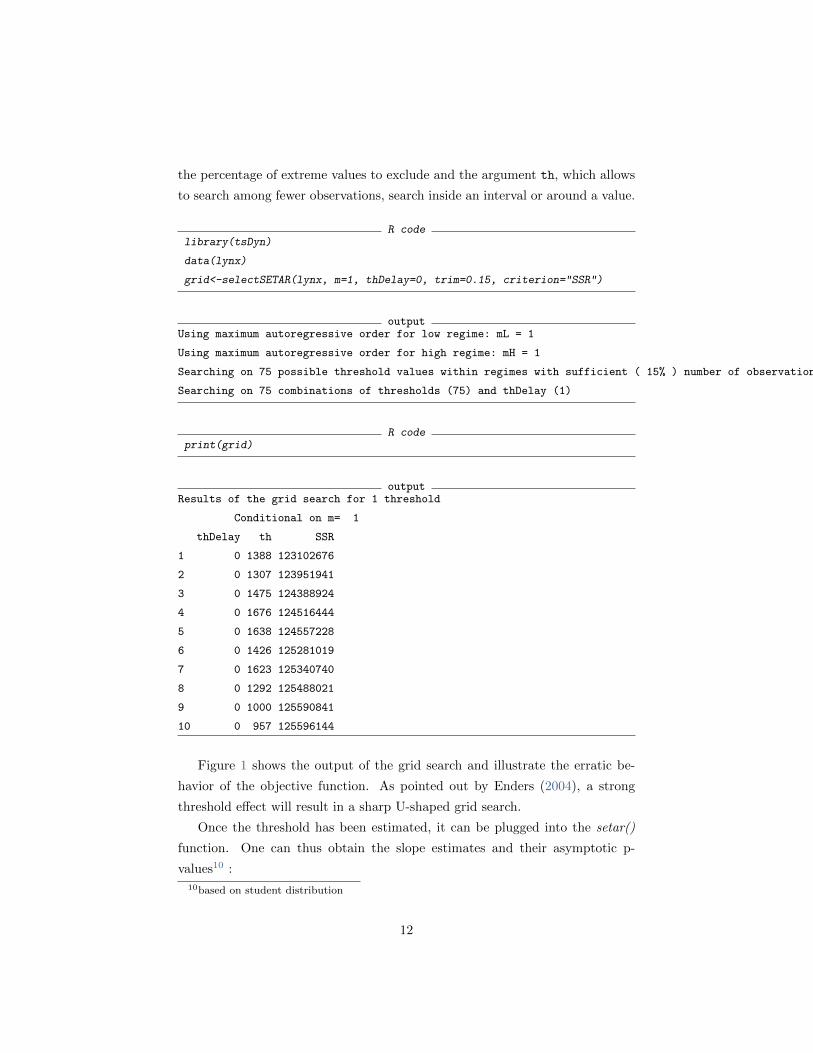
the percentage of extreme values to exclude and the argument th, which allows

to search among fewer observations, search inside an interval or around a value.

R codelibrary(tsDyn)

data(lynx)

grid<-selectSETAR(lynx, m=1, thDelay=0, trim=0.15, criterion="SSR")

outputUsing maximum autoregressive order for low regime: mL = 1

Using maximum autoregressive order for high regime: mH = 1

Searching on 75 possible threshold values within regimes with sufficient ( 15% ) number of observations

Searching on 75 combinations of thresholds (75) and thDelay (1)

R codeprint(grid)

outputResults of the grid search for 1 threshold

Conditional on m= 1

thDelay th SSR

1 0 1388 123102676

2 0 1307 123951941

3 0 1475 124388924

4 0 1676 124516444

5 0 1638 124557228

6 0 1426 125281019

7 0 1623 125340740

8 0 1292 125488021

9 0 1000 125590841

10 0 957 125596144

Figure 1 shows the output of the grid search and illustrate the erratic be-

havior of the objective function. As pointed out by Enders (2004), a strong

threshold effect will result in a sharp U-shaped grid search.

Once the threshold has been estimated, it can be plugged into the setar()

function. One can thus obtain the slope estimates and their asymptotic p-

values10 :

10based on student distribution

12

Figure 1: Graphical output of the grid search for one threshold

R codeplot(grid)

●●●●●●●●

●●●●●●●●●

●●

●●●●

●

●●

●●

● ●

●

●

●

●

●

●●●●●

●●

●●

●

●

●

●

●

●

●

●

●

●●

●

●●

●●

●●

●

●●

●

●

●●●

●

●

●

●●

500 1000 1500 2000 2500 3000

1.24

e+08

1.28

e+08

1.32

e+08

Threshold Value

SS

R

Results of the grid search

●

●

●

Threshold Delay 0th 1

13

R codeset<-setar(lynx, m=1, thDelay=0, th=grid$th)

summary(set)

outputNon linear autoregressive model

SETAR model ( 2 regimes)

Coefficients:

Low regime:

const.L phiL.1

-150.298119 1.997857

High regime:

const.H phiH.1

984.5047382 0.5595309

Threshold:

-Variable: Z(t) = + (1) X(t)

-Value: 1388 (fixed)

Proportion of points in low regime: 59.29% High regime: 40.71%

Residuals:

Min 1Q Median 3Q Max

-2677.749 -471.918 90.273 327.865 4067.721

Fit:

residuals variance = 1079848, AIC = 1592, MAPE = 119.8%

Coefficient(s):

Estimate Std. Error t value Pr(>|t|)

const.L -150.29812 220.45996 -0.6817 0.49683

phiL.1 1.99786 0.39437 5.0659 1.651e-06 ***

const.H 984.50474 385.10377 2.5565 0.01194 *

phiH.1 0.55953 0.11439 4.8915 3.442e-06 ***

---

Signif. codes: 0

14

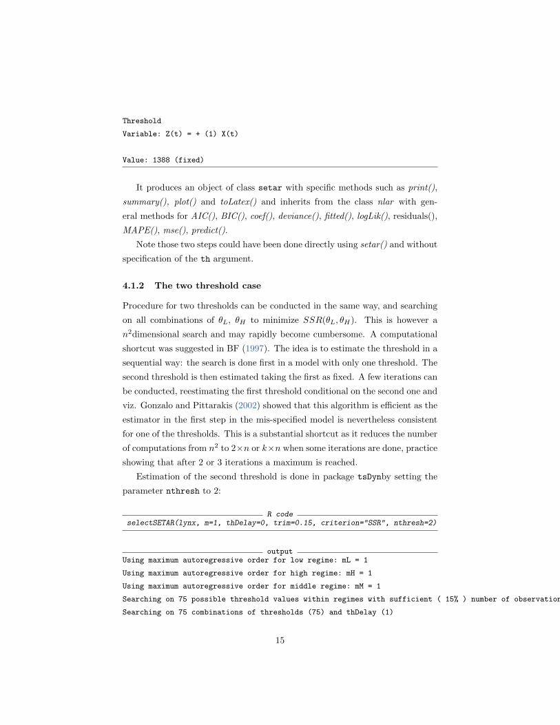
Threshold

Variable: Z(t) = + (1) X(t)

Value: 1388 (fixed)

It produces an object of class setar with specific methods such as print(),

summary(), plot() and toLatex() and inherits from the class nlar with gen-

eral methods for AIC(), BIC(), coef(), deviance(), fitted(), logLik(), residuals(),

MAPE(), mse(), predict().

Note those two steps could have been done directly using setar() and without

specification of the th argument.

4.1.2 The two threshold case

Procedure for two thresholds can be conducted in the same way, and searching

on all combinations of θL, θH to minimize SSR(θL, θH). This is however a

n2dimensional search and may rapidly become cumbersome. A computational

shortcut was suggested in BF (1997). The idea is to estimate the threshold in a

sequential way: the search is done first in a model with only one threshold. The

second threshold is then estimated taking the first as fixed. A few iterations can

be conducted, reestimating the first threshold conditional on the second one and

viz. Gonzalo and Pittarakis (2002) showed that this algorithm is efficient as the

estimator in the first step in the mis-specified model is nevertheless consistent

for one of the thresholds. This is a substantial shortcut as it reduces the number

of computations from n2 to 2×n or k×n when some iterations are done, practice

showing that after 2 or 3 iterations a maximum is reached.

Estimation of the second threshold is done in package tsDynby setting the

parameter nthresh to 2:

R codeselectSETAR(lynx, m=1, thDelay=0, trim=0.15, criterion="SSR", nthresh=2)

outputUsing maximum autoregressive order for low regime: mL = 1

Using maximum autoregressive order for high regime: mH = 1

Using maximum autoregressive order for middle regime: mM = 1

Searching on 75 possible threshold values within regimes with sufficient ( 15% ) number of observations

Searching on 75 combinations of thresholds (75) and thDelay (1)

15

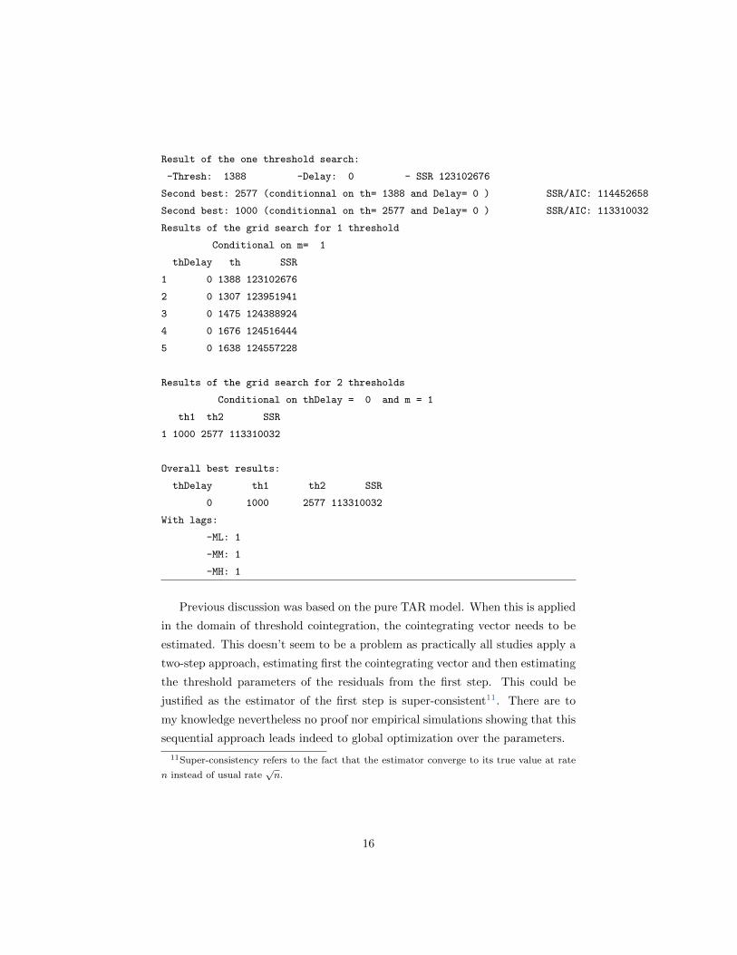
Result of the one threshold search:

-Thresh: 1388 -Delay: 0 - SSR 123102676

Second best: 2577 (conditionnal on th= 1388 and Delay= 0 ) SSR/AIC: 114452658

Second best: 1000 (conditionnal on th= 2577 and Delay= 0 ) SSR/AIC: 113310032

Results of the grid search for 1 threshold

Conditional on m= 1

thDelay th SSR

1 0 1388 123102676

2 0 1307 123951941

3 0 1475 124388924

4 0 1676 124516444

5 0 1638 124557228

Results of the grid search for 2 thresholds

Conditional on thDelay = 0 and m = 1

th1 th2 SSR

1 1000 2577 113310032

Overall best results:

thDelay th1 th2 SSR

0 1000 2577 113310032

With lags:

-ML: 1

-MM: 1

-MH: 1

Previous discussion was based on the pure TAR model. When this is applied

in the domain of threshold cointegration, the cointegrating vector needs to be

estimated. This doesn’t seem to be a problem as practically all studies apply a

two-step approach, estimating first the cointegrating vector and then estimating

the threshold parameters of the residuals from the first step. This could be

justified as the estimator of the first step is super-consistent11. There are to

my knowledge nevertheless no proof nor empirical simulations showing that this

sequential approach leads indeed to global optimization over the parameters.

11Super-consistency refers to the fact that the estimator converge to its true value at rate

n instead of usual rate√n.

16

4.1.3 Distribution of the estimator

Properties of the concentrated LS estimator described above were obtained by

Chan (1993). He established that the estimator of the threshold, θ, was super-

convergent, whereas the estimator of the slope coefficients, β, was convergent.

He furthermore found that the distribution of θ is a compound Poisson process

with nuisance parameters, which can’t be computed easily. Superconvergence

of θ allows asymptotically to take the estimated value as given and conduct

usual inference on the β. Indeed, the distribution of β is the usual gaussian law

and is independent asymptotically of the θ. Those results apply when all the

coefficients values differ in each regime, the distribution of the whole process

being discontinuous. In a certain case when only a few variables have regime

specific value, the so-called continuous case, Chan and Tsay (1998) established

that the threshold estimator converges at the usual rate and is normally dis-

tributed, whereas the asymptotic Independence does not hold. However, the

continuous model does not seem to have received much use in empirical appli-

cations12. There remains an uncertainty for me nevertheless if some studies use

actually a continuous model but describing it as a discontinuous model.

Note that while in both continuous and discontinuous models the results are

known in the one threshold case, there is to my knowledge no study investigating

the two thresholds model.

Inference on the threshold parameters A few studies have concentrated

on methods to do inference on the threshold parameter. Hansen (2000) makes

the assumption that the threshold effect vanishes asymptotically, which enables

him to derive the distribution of the threshold parameter and to provide critical

values for the likelihood ratio test of θ = θ0. Confidence intervals can then

be obtained by inverting the log-likelihood ratio: the bound are the values for

which the test is rejected. 13

Gonzalo and Wolf (2005) use a subsampling procedure to obtain confidence

intervals for the threshold. Their method has the advantage of providing a test

to discriminate between continuous and discontinuous models. Seo and Linton

12Gonzalo and Wolf (2005) discuss a test to differentiate between continuous and discon-

tinuous model.13As the objective function is erratic, there may be intervals inside which the test was

rejected for some values and not rejected for others, see graph page 588 in Hansen (2000).

17

(2007) modify the objective function by replacing the indicator function by a

smoothing function14. This so called smoothed least square estimator has a

smaller rate of convergence but is normally distributed and still independent

of the slope parameter estimator. They furthermore establish the validity of

a regressor-based bootstrap to obtain small-sample refinements. None of those

methods is currently implemented in package tsDyn, but the inclusion of Hansen

method is under project.

Even if the estimators of the slope parameters are asymptotically normally

distributed and independant of the threshold estimator, this may not hold in

small sample. Hansen (2000), and Seo and Linton (2006), both suggest methods

to take into account the variability of the threshold parameter when building

confidence intervals for the slope coefficients. Hansen’s method requires lot of

computations as it implies to estimate the confidence interval of β(θ) for all θi

that are included in the confidence interval of θ. Using the normality of the

smoothed-least square, Seo and Linton (2006) are able to obtain a simpler way

to compute the confidence interval for β.

-Carlo Studies Globally, Monte Carlo studies of the estimators in the pre-

vious papers (Hansen 2000, Gonzalo and Wolf 2005, Seo and Linton 2006) find

that the threshold parameters exhibit a large variability, higher than is predicted

by the asymptotical theory: super-convergence of the estimator does not seem

to be effective in small samples. Consequently, the slope estimators exhibit a

large variability. Without surprise, the authors remark that the variability de-

crease with the sample size as well as with the effect threshold: the bigger the

difference in the parameters in each regime, the better the estimation of the

threshold. Gonzalo and Pittarakis (2002) find another interesting factor influ-

encing the variability, namely the number of observations in each regime. While

it seems obvious that this will influence the precision in estimating the slope

parameters, they show that this affects also the threshold parameter. Indeed,

θ is best estimated when there are an equal number of observations in each

regime, precision of the estimator decreasing when only a few observations are

present in a regime.

14This can be a distribution function as it needs to be bounded between 0 and 1.

18

Estimation of the number of lags The estimation of the number of lags

can be done be using again the concentration method given above, using as

objective function an information criterion (AIC, BIC) rather than the SSR.

IC() = n ∗ log σ2ε + a(n) ∗ k (9)

Where a(n) =2 for the Akaike information criterion (AIC) or a(n)=ln(n) for

the bayesian information criterion (BIC)15.

The parameter are then

(θ1,, θ2,, k1,, k2,, k3, = arg min IC(θ1, θ2, k1, k2, k3) (10)

This is a considerable extension of the dimension of the grid search, and

usually one uses the restriction k1 = k2.

This is possible in package tsDynby specifying the argument criterion=AIC

in function selectSETAR():

R codeselectSETAR(lynx, m=6, thDelay=0, trim=0.15, criterion="AIC", same.lags=TRUE)

outputUsing maximum autoregressive order for low regime: mL = 6

Using maximum autoregressive order for high regime: mH = 6

Searching on 70 possible threshold values within regimes with sufficient ( 15% ) number of observations

Searching on 420 combinations of thresholds ( 70 ), thDelay ( 1 ) and m ( 6 )

Results of the grid search for 1 threshold

thDelay m th AIC

1 0 2 1388 1528.278

2 0 2 1307 1528.471

3 0 2 808 1529.596

4 0 2 1000 1529.765

5 0 2 1033 1529.830

6 0 2 1292 1529.882

7 0 2 1132 1529.940

8 0 2 957 1530.249

9 0 2 784 1530.425

10 0 2 758 1530.807

15There are several formulations of those criterions. We took here the formulation as in

Franses and van Dijk (2000)

19

The argument same.lags restrict the search to have the same number of

lags in each regime. Its default value, currently set to FALSE16, search on all

combinations of lags, that is, allows to have different lags in each regime.

4.2 Estimation and inference in the TVECM representa-

tion

Estimation Estimation of the threshold and cointegrating parameters could

be done in the long-run relationship and those estimates plugged into the TVECM,

as the Engle-Granger advocates for the linear case. To my knowledge,the the

validity of that method has not been investigated in theoretically. BF mention

that the super-convergence of the OLS estimator in the LR (Watson 1987) still

hold when the residuals follow a SETAR process under the condition (1).

Rather, Hansen and Seo (2002) and Seo (2009) study estimators directly

based on the TVECM. Hansen and Seo derive a maximum-likelihood (ML) es-

timator, and use a two-dimensional grid for simultaneous estimation of θ and γ.

This two-dimensionality can’t be avoided as the parameters can’t be expressed

as functions each of the other one: for each cointegrating value the ECT will

be different. For θ, the grid is restricted to the existing values of the ECT,

with exclusion of the upper and lower ranges. For the cointegrating value, HS

suggest to conduct the search based on a confidence interval obtained in the

linear model. When the two values are give, the slope and speed adjustment

parameters can be concentrated out and the estimator is simply OLS (though

HS depict it as MLE, it is only MLE as starting values for the algorithm are

based on the linear MLE estimate). This method can be done in a simple bi-

variate model without intercept in the cointegrated relationship, but becomes

intractable with more than two cointegrating relationships.

Note that in what I called the cointegration with threshold effect framework,

where an external variable rather than the ECT is taken as transition variable,

estimation is highly simplified as the interdependency between the ECT term

and the threshold variable is ruled out. Estimation of multivariate VECM with

many cointegrating relationships is then feasible, the grid search being conduced

only over the threshold parameter space (Krishnakumar and Netto 2009).

16This will probably be changed soon in future version.

20

Inference While Hansen and Seo (2002) suggested an estimator for the mul-

tivariate case, they only conjectured its consistency. Interesting results can

be found in Seo (2009) concerning proprieties of the LS estimator. Seo shows

that LS estimators of both the threshold and cointegrating values are super

convergent, the estimator β converging at a faster rate than in linear model, at

n32 instead of n. Similarly as in his previous work in the univariate case (Seo and

Linton 2007), Seo considers a smoothed-LS estimator and finds that is converg-

ing at a slower rate but then normally distributed, allowing to obtain confidence

intervals.

Implementation in R The function TVECM() in package tsDynallows to

estimate a bivariate TVECM with two or three regimes with the OLS like es-

timator. It should be emphasized here that in my view there is no difference,

except in the starting value, between the OLS and MLE estimator, as condi-

tional on the threshold and the cointegrating value, the MLE estimator is simply

LS. The model can be specified either with a constant a trend, or none, (arg

include) and the lags can be regime specific or not (arg common).

Procedure for the TVECM() differ from that of setar() as there is no cor-

responding selectSETAR() function. As the search is two dimensional and the

cointegrating parameter take continuous values, it can be easily cumbersome

and different options to restrict the search are given with arguments ngrid-

Beta, ngrid, Th, gamma1, gamma2, beta17.

R codedata(zeroyld)

tvecm<-TVECM(zeroyld, nthresh=2,lag=1, ngridBeta=60, ngridTh=30, plot=TRUE,trim=0.05, beta=list(int=c(0.7, 1.1)))

It produces an object of class TVECM() with specific methods such as

print(), summary() and toLatex() and inherits from the class nlVar with general

methods for AIC(), BIC(), coef(), deviance(), fitted(), logLik(), residuals().

Note that a plot of the search is given automatically as this has proved in

practice to be a useful tool, experience showing that the confidence interval

for the cointegrating values are too small and hence only a local minimum is

obtained, which can be easily detected with the plot.

17Name of this argument will probably be modified in further version of the package.

21

Figure 2: Results of the two-dimensional grid search for a TVECM

−1.5 −1.0 −0.5 0.0 0.5 1.0 1.5

155

165

Grid Search

Threshold parameter gamma

Res

idua

l Sum

of S

quar

es

●

0.7 0.8 0.9 1.0 1.1

155

165

Cointegrating parameter beta

Res

idua

l Sum

of S

quar

es

OLS estimate from linear VECM

22

5 Testing

Testing for threshold cointegration is particularly difficult as it involves two

aspects: the presence of cointegration and that of non-linearity. Hence, one

may have four different cases:

� Cointegration and threshold effects

� Cointegration and no threshold effects

� No cointegration and no threshold effects

� No cointegration and threshold effects

Hence, a test with threshold cointegration may have as null hypothesis either

cointegration or no cointegration. This distinction is of major importance as this

implies a different distribution under the null. The distribution is also different

whenever the test is done based on the LR or the VECM representation18. Some

of the tests also allow to estimate the cointegrating vector, whereas the majority

requires pre-specified ones. Finally, the number of regime differ in the different

specifications, some taking two, some three regimes, or symmetric outer regimes.

To my knowledge, only one test (Hansen 1999) is able to determine the number

of regimes, through a test of one against two thresholds. As a result, there exist

many different tests for all the possible cases.

The approach advocated by BF was to conduct a two-step analysis in the LR

with pre-specified cointegrating value: testing first for cointegration, and if tests

indicate presence of cointegration to test for threshold effects. Nevertheless, this

approach may suffer of low power when the true model contains threshold effects

and the first step is conduced using tests with a linear specification. Indeed,

several studies showed that conventional unit root tests had very low power

when the alternative was a stationary SETAR (Pippenger and Goering 2000).

Indeed, many studies found that the LOP did not hold, the unit root being not

rejected, contrary to many economic arguments in favor of its stationarity.

Taylor (2001) advocated that the failure of tests to reject the unit root for

the case of the LOP was due to the use of test which assume linear adjustment.

Use of more appropriate tests was indeed able to confirm the LOP. He showed

18Actually a VAR if the null is no cointegration.

23

through theoretical and simulation-based arguments that indeed linear tests

were biased towards non-rejection of stationarity.

Hence, the procedure should be to do, as in BF, a two-step approach, using

first linear tests of cointegration. If linear cointegration is not rejected, tests for

threshold cointegration with linear under H0should be used. Failure of cointe-

gration in the first step should lead to the use of tests with no cointegration

under H0and threshold cointegration under the alternative. The second case is

particularly interesting, as it illustrates how threshold cointegration is a broader

concept that involves linear cointegration as a specific case.

5.1 The problem of the unidentified parameter

A problem for the statistical testing procedure arises when the threshold pa-

rameter needs to be estimated. In case of a known threshold parameter, a

likelihood-ratio test for the null of no threshold effects (testing actually equality

of the coefficients in each regime) can be formed and has the usual χ2 distri-

bution (Chan and Tong 1990). But when it is unknown, which is typically the

case in practice19, the distribution of the test is then non-standard as it entails

a parameter that is not identified under the null, the so-called Davies problem

(1977, 1987).

Solutions for that problem (Andrews and Ploberger 1994) involve usually

applying the test statistic for a wide range of possible threshold values, and

then aggregating those results. One of the solution encountered is to average all

the values, either by using a simple mean or an exponential average. Another

solution is to use a supremum statistic, that is the value for which the test is

most favorably rejected. This may be seen as an endogeneity bias, but it is not

as long as appropriate asymptotical tools are used, that take into account this

variability of the test. For a discussion on that question in the similar field of

structural break, see Perron (1989) and Andrews and Zivot (1992).

As the test are applied on a range of values, the question of the selection

of that range arises. A typical approach is to sort the threshold values in as-

cending order and exclude a certain percentage of the lowest and highest values.

There is no clear rule on the choice of this percentage, but it should not be too

small as Andrews and Ploberger (1994) show that setting it too low result in

a considerable size distortion. Other approaches as in Bec et al. (2008) is to

19unless maybe when one imposes a threshold of zero

24

construct a different grid under the null and under the alternative, using the

ADF unit root test for the pre-testing.

The sup-test procedure looks really similar to the estimation procedure as

both rely on the use of a sorted grid, with exclusion of some extreme values. The

parameter selected nevertheless is the same only in the case of an homoscedastic

Wald (or Fisher) test. Indeed, the threshold parameter minimizing the SSR need

not be the same of that one maximizing a LM statistic.

Another interesting approach is provided in Altissimo and Corradi (2002)

who derive bounds for Wald and LM type tests. Contrary to the usual approach

consisting in deriving the asymptotical distribution of the tests and obtaining

critical values, they simply show that one may apply a functional to the test

that is bounded.

The decision rule from their bound is easy as the model under the null (al-

ternative) should be chosen when the bound is below (above) one. They show

that this procedure leads to type I and type II errors approaching zero asymp-

totically. This result is of great importance as it allows to reduce substantially

the number of computation, as critical values don’t need to be tabulated.

5.2 Cointegration vs. threshold cointegration tests

5.2.1 Test based on the long-run relationship

As discussed above, the idea for the testing procedure if to test first for coin-

tegration and in the case when cointegration is not rejected, test for threshold

cointegration, taking cointegration as a null. In our view, implicetly assumed in

that methodology is that the threshold model will be also stationary. Whereas

the fact that a unit root may appear in a three-regime SETAR model, the ques-

tion is never asked in a two regimes-model. This is an important gap as indeed

splitting the sample may create a unit root in one of the regime. This is the

case indeed in Hansen (1999), who did not seem to note it.

In package tsDyn, a minimal test is done automatically computing whether

the roots of the polynomials don’t have values equal or lower to one. Hence,

one obtains an automatical warning with data from Hansen (1999):

R codedata(IIPUs)

set<-setar(IIPUs, m=16, thDelay=5, th=0.23)

25

Hansen (1996) derived the asymptotic properties of the sup-LM test for

a SETAR model with one unknown threshold. The test follows a complicated

empirical distribution process with nuisance parameters and hence critical values

for a general case can’t be tabulated. Hansen nevertheless shows a simulation

procedure which allows to generate asymptotic p-values. In this procedure,

heteroskedasticity can also be taken into account by slight modifications. In a

later article, Hansen (1999) studies an alternative way to obtain the p-values

through a residual bootstrap, whose validity is nevertheless not established but

only conjectured. More interestingly, the author develops an extension of the

testing procedure to test against two threshold, and to determinate the number

of thresholds by testing the null of one threshold against two.

This test is available in tsDynwith the function setarTest(), for which the

homoskedastic bootstrap have been implemented. It takes as argument nboot

the number of bootstrap replications and test=”1vs” (1 regimes against 2) or

”2vs3” (2 regimes against 3).

R codeHansen.Test<-setarTest(lynx, m=1, nboot=1000)

Available methods are print(), summary() and plot(), as well as an extend-

Boot() function to run new bootstrap replications and merge the result with the

old ones. This can be useful for a preliminary test and to check how the result

is influenced by new runs.

Another type of test has been suggested by Petrucelli and Davies (1986) and

Tsay (1989). By transforming the specification into an arranged autoregression,

Tsay reformulates the problem into a structural change test. With a test of

stability of recursive residual to detect structural change, the problem of the

unidentified parameter under H0 is avoided and hence the test follows a simple

χ2distribution. This test has been implemented in R but not included in version

0.7 as the result differ sometimes drastically from those in the paper20

BF suggested to extend the approach of Tsay using several other structural

change tests, using techniques as in Hansen (1996). Appropriateness of this

method has been nevertheless discussed by Hansen (2000) as the the ordering

of the variable for the arranged autoregression may induce a trend, in case the

structural tests are not consistent.20actually as well as from those also differing in the GAUSS procedure distributed by Lo

and Zivot (2002).

26

Criterion based approaches Differing from a pure testing procedure, model

selection procedures based on information criteria (IC) have gained much inter-

est in the literature and their use has been sometimes advocated rather than

formal testing procedure (see for example Letkephol2007). This is the case in

the well-known selection of lags in time series models, but also for estimating

the cointegrating rank (Gonzalo and Pittarakis 1998, Cheng and Phillips2009).

This has been also applied for the determination of the number of regimes

in a SETAR model by Gonzalo and Pittarakis (2002). They show indeed that

this works well in practice using a modified BIC. This result is of great interest

in practice as it avoids the use of bootstrap replications and hence significantly

diminishes the number of computations required. The authors remark in sim-

ulations studies that the AIC has big type one error compared to other BIC,

while it has a smaller type II error.

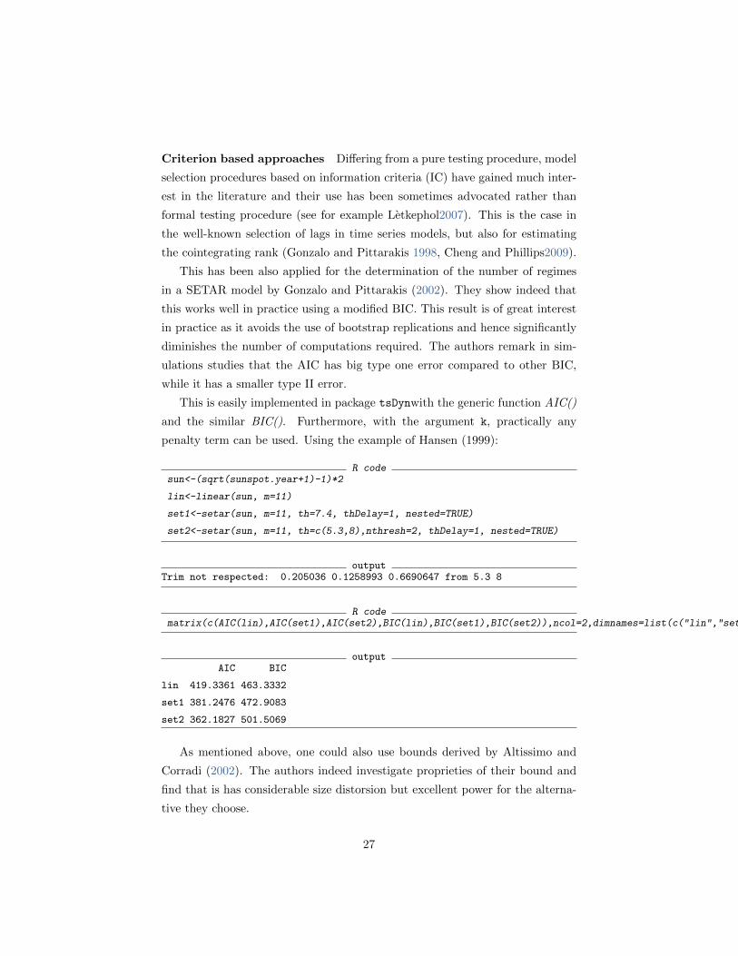
This is easily implemented in package tsDynwith the generic function AIC()

and the similar BIC(). Furthermore, with the argument k, practically any

penalty term can be used. Using the example of Hansen (1999):

R codesun<-(sqrt(sunspot.year+1)-1)*2

lin<-linear(sun, m=11)

set1<-setar(sun, m=11, th=7.4, thDelay=1, nested=TRUE)

set2<-setar(sun, m=11, th=c(5.3,8),nthresh=2, thDelay=1, nested=TRUE)

outputTrim not respected: 0.205036 0.1258993 0.6690647 from 5.3 8

R codematrix(c(AIC(lin),AIC(set1),AIC(set2),BIC(lin),BIC(set1),BIC(set2)),ncol=2,dimnames=list(c("lin","set1", "set2"),c("AIC", "BIC")))

outputAIC BIC

lin 419.3361 463.3332

set1 381.2476 472.9083

set2 362.1827 501.5069

As mentioned above, one could also use bounds derived by Altissimo and

Corradi (2002). The authors indeed investigate proprieties of their bound and

find that is has considerable size distorsion but excellent power for the alterna-

tive they choose.

27

This bound has not been implemented in tsDynas results were different com-

pared to other studies (see Galvao 2006) and there is no comparison of the results

with other testing procedures.

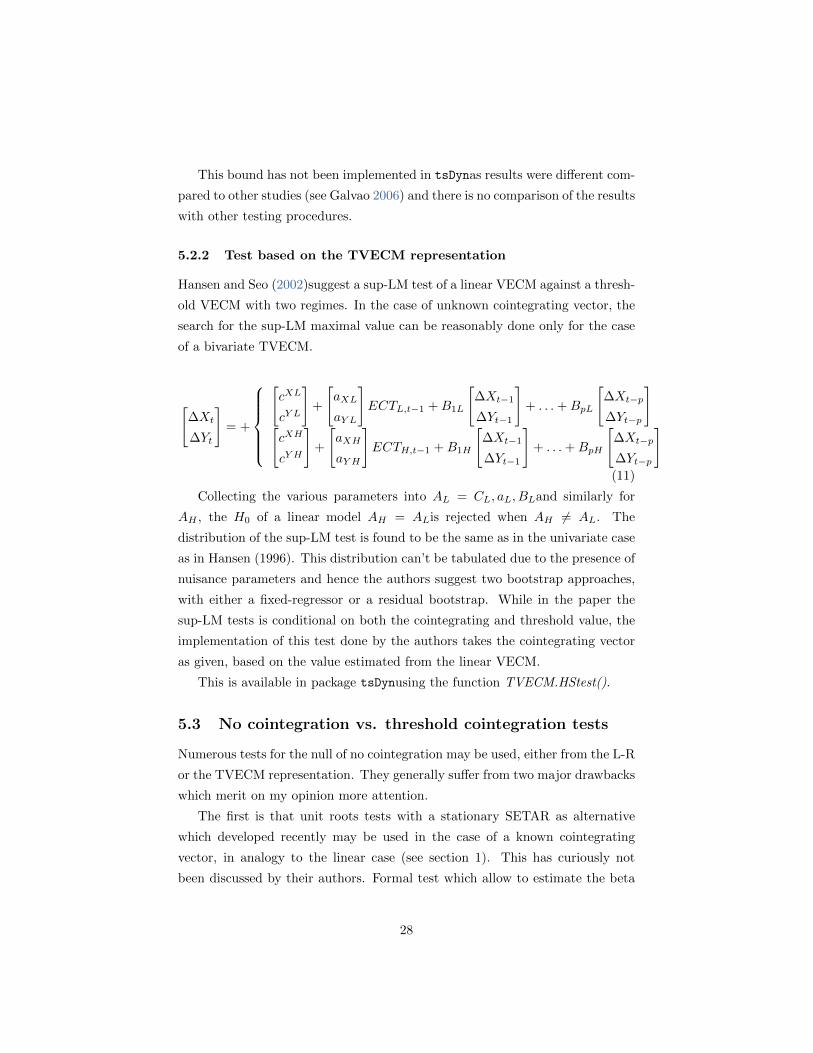
5.2.2 Test based on the TVECM representation

Hansen and Seo (2002)suggest a sup-LM test of a linear VECM against a thresh-

old VECM with two regimes. In the case of unknown cointegrating vector, the

search for the sup-LM maximal value can be reasonably done only for the case

of a bivariate TVECM.

[∆Xt

∆Yt

]= +

[cXL

cY L

]+

[aXL

aY L

]ECTL,t−1 +B1L

[∆Xt−1

∆Yt−1

]+ . . .+BpL

[∆Xt−p

∆Yt−p

][cXH

cY H

]+

[aXH

aY H

]ECTH,t−1 +B1H

[∆Xt−1

∆Yt−1

]+ . . .+BpH

[∆Xt−p

∆Yt−p

](11)

Collecting the various parameters into AL = CL, aL, BLand similarly for

AH , the H0 of a linear model AH = ALis rejected when AH 6= AL. The

distribution of the sup-LM test is found to be the same as in the univariate case

as in Hansen (1996). This distribution can’t be tabulated due to the presence of

nuisance parameters and hence the authors suggest two bootstrap approaches,

with either a fixed-regressor or a residual bootstrap. While in the paper the

sup-LM tests is conditional on both the cointegrating and threshold value, the

implementation of this test done by the authors takes the cointegrating vector

as given, based on the value estimated from the linear VECM.

This is available in package tsDynusing the function TVECM.HStest().

5.3 No cointegration vs. threshold cointegration tests

Numerous tests for the null of no cointegration may be used, either from the L-R

or the TVECM representation. They generally suffer from two major drawbacks

which merit on my opinion more attention.

The first is that unit roots tests with a stationary SETAR as alternative

which developed recently may be used in the case of a known cointegrating

vector, in analogy to the linear case (see section 1). This has curiously not

been discussed by their authors. Formal test which allow to estimate the beta

28

have not been derived in the L-R nor in TVECM form, and hence constrain the

threshold cointegration field to analyze only cases where the cointegrated values

are meant to be known. Even if it is a strong restriction, it is still interesting,

since there are many applications where theory predicts a particular cointegrated

vector, as Horvath and Watson (1995) claim:

Economic models often imply that variables are cointegrated with

simple and known cointegrating vectors. Examples include the neo-

classical growth model, which implies that income, consumption, in-

vestment, and the capital stock will grow in a balanced way, [...]. As-

set pricing models with stable risk premia imply corresponding stable

differences in spot and forward prices, long- and short-term interest

rates, and the logarithms of stock prices and dividends. Most the-

ories of international trade imply long-run purchasing power parity,

so that long-run movements in nominal exchange rates are matched

by countries relative price levels. Certain monetarist propositions

are centered around the stability of velocity, implying cointegration

among the logarithms of money, prices, and income.

A second drawback of the test with the null of no cointegration is that the

alternative stationary model always take the form of the condition (1). Hence,

the presence of a unit root is considered as non-stationarity of the series. We

saw nevertheless above that a SETAR process may still be stationary even with

a unit root in a regime. Henceforth, the non-rejection towards stationarity

is not in itself a sign that the series is indeed non-stationary. It is only a

first step indicating that condition (1) of stationarity does not hold, but this

does not mean that other conditions may not hold and the process hence be

stationary. However, those further investigations are not possible as there are

to my knowledge no tests that take as alternative hypothesis other conditions

such as (2) or (3). We may hence conjecture that many of the series described

as non-stationary in the literature may well be SETAR-stationary.

5.3.1 Tests based on the long-run relationship

Taking no cointegration as null hypothesis has the implication that under the

null, the series (which is also, remember, the transition variable) is non-stationary,

which affects the distribution of the tests. Analogously as in the linear case,

29

when the cointegrating vector is known, usual unit root tests can be used,

whereas estimation of the cointegrating vector affect the distribution of the

test, which require use of different tests/critical values. Hence, when the cointe-

grating vector is known, unit root tests with a stationary SETAR as alternative

can be used, whereas the case of unknown cointegrating vector needs correction.

Known threshold

Bec, Ben Salem and Carrasco (BBC) Bec, Ben Salem and Carrasco

(2004) (referred as to BBC), test for unit root against a symmetric three regime

SETAR model. The model specification is very general as intercepts as well as

lags are included in each regime, and hence corresponds to the model in 7.

∆yt = IL

(µL + ρLyt−1 +

∑∆γL,iyt−i

)IM

(µM + ρMyt−1 +

∑∆γM,iyt−i

)IH

(µH + ρHyt−1 +

∑∆γH,iyt−i

)+εt

(12)

where IL = I{yt−1≤−θ}, IH = I{yt−1>θ} and IM = I{−θ≤yt−1≤θ}

The null hypothesis of unit root is H0: ρL = ρH = ρM = 0 with the

alternative HA: ρL < 1, ρH < 0 and ρM ≤ 1. That is, a unit root is allowed in

the middle regime, but an explosive behavior is ruled out. BBC find that the

distribution of sup-Wald, sup-LM and sup-LR are free of nuisance parameters

and provide critical values. The authors suggest that the extension to a SETAR

with non symmetric thresholds should not lead to further complications.

Kapetanios and Shin (KS) Kapetanios and Shin (2006) uses as alternative

a three-regime model with a unit root in the inner middle which is meant to

be more consistent with the concept of a band without adjustment. As then

coefficients in the middle regime do not need to be estimated, the test is meant

to have better power when the true model is indeed a model with a unit root

in the inner regime. They allow the possibility to add lags common to all the

regimes.

∆yt = µL + ρLyt−1 + µH + ρHyt−1 +

p∑i=1

γi∆yt−i + εt (13)

The null hypothesis of unit root is H0: ρL = ρH = 0 with the alternative

HA: ρL < 1, ρH < 0. The grid for the thresholds is selected such that the

probability of being in the middle regime decreases as the sample size increases,

30

converging to zero asymptotically. Under this specification, the authors derive

statistics (the sup-Wald, exp Wald and ave Wald) which are obtain nuisance

parameter free and provide critical values.

Bec, Guay and Guerre (BGG) Under a similar model such as in BBC,

Bec, Guay and Guerre (2008) (hereafter BGG) concentrate on the selection of

the grid to obtain a consistent test diverging under HA. The idea is that if H0

is true, the grid should be small as to ensure a good size, whereas if HA holds,

the grid should be as large as possible to ensure power. Hence, the width of the

grid is selected depending on a pre-test based on the AD test.

Seo Seo (2008) derive a test with a two-regime SETAR as alternative, allowing

for non linear and serial correlated errors. Under those weaker assumptions,

the asymptotical distribution of the sup-Wald selecting the values as in KS

depends on nuisance parameters and critical values can’t be tabulated. Seo

hence suggests a residual based block bootstrap, shown to be asymptotically

consistent. Extension of the bootstrap for a three regime model is meant to be

easy.

Monte Carlo comparisons Maki (2009) provides a Monte Carlo simulation

for the size and power of the BBC (using sup-Wald) and KS (sup-Wald, ave and

exp-Wald) tests, along with the traditional ADF. Size of the test is definitely

better for the ADF test, with the ave-Wald being close, the sup- and exp-Wald

of KS showing size distorsion, while the sup-wald of BBC is seen to be too

conservative. Power of the tests is investigated based on an alternative model

with three regimes, a symmetric threshold, a unit root in the middle regime

and no lags. Different values of the thresholds are tested. With a threshold

value of zero (i.e. no thresholds effects), the ADF test has without surprise the

best power. More surprisingly, this is still the case with small thresholds, with

values 1 and 2, the ADF test having the best power for models with an inner

regime counting 40% of the observations. When the thresholds increase (and

hence the number of observations in the unit root regime), power of the ADF

decreases consequently. This is also the case for the KS test, as it is based on

a asymptotically degenerated threshold, whereas there is no clear effect on the

BBC. As the KS test does not estimate the inner regime whereas the BBC does,

31

the power of the KS is much higher, because the true process has indeed a unit

root.

When the mean-reversion of the outer regime is increased (which has the

effect to have more observations in the inner regime), all the tests have power

near to 1 unless the threshold are high (value of 6), where power of ADF test

falls. The BBC test has in those cases a much better power than the KS, as the

latter is based on a diminishing threshold effect.

Implementation in R BBC and KS have been implemented in package ts-

Dyn. They are nevertheless for now in an experimental version and may contain

errors. Practitioners should use them with care as the results could not be

compared to those of the authors as the data sets are not publicly available.

5.3.2 Unknown cointegrating values

Two early tests deserve here mention. Enders and Granger (1998) first provided

an empirical framework to deal with unit root tests having a two-regime SETAR

as alternative. They tabulated critical values for a test when the threshold is

known. Critical values with unknown threshold were given later by Enders

(2001). Enders and Siklos (2001) adopt similar approach but relying on the

cointegration framework and allowing to estimate the cointegrating values. They

hence provide larger critical values from those of Enders and Granger (1998).

This is to my knowledge the only test which allows to work with an unknown

cointegrating vector. It is not sure nevertheless whether it more appropriate to

use this one rather that the more formal unit root tests of BBC and KS, as no

distribution theory is given in the former.

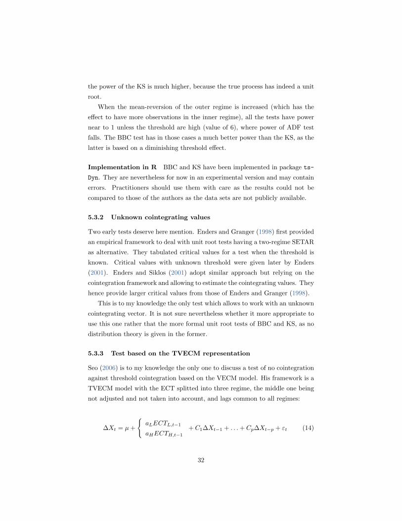
5.3.3 Test based on the TVECM representation

Seo (2006) is to my knowledge the only one to discuss a test of no cointegration

against threshold cointegration based on the VECM model. His framework is a

TVECM model with the ECT splitted into three regime, the middle one being

not adjusted and not taken into account, and lags common to all regimes:

∆Xt = µ+

{aLECTL,t−1

aHECTH,t−1+ C1∆Xt−1 + . . .+ Cp∆Xt−p + εt (14)

32

The idea of the test is based on results as in Horvath and Watson (1995), who

show that when the cointegrating vector is known, a test of cointegration can

be simply done on testing whether coefficients from the ECT are significant.

In the TVECM framework, the null hypothesis of no cointegration becomes:

H0: aL = aH = 0 and the alternative that either aL or aH is different from

zero. The sup-Wald test suggested does not depend on nuisance parameter

and critical values can be obtained. As the asymptotical distribution is seen

to perform badly in small samples, Seo provide a residual based bootstrap and

shows its asymptotic consistency.

This test is available in package tsDynas TVECM.SeoTest().

R codedata(zeroyld)

dat<-zeroyld

testSeo<-TVECM.SeoTest(dat, lag=1, beta=1, nboot=1000)

summary(testSeo)

It requires the argument beta for the cointegrating value and nboot for the

number of bootstrap replications. The methods print(), summary() and plot()

are available for objects issued by TVECM.SeoTest(). As the model specification

is done for two thresholds, a two-dimensional grid search has been implemented.

This is definitely very slow and a single test may take a few hours 21.

5.4 Conclusion for the test

I reviewed here some of the most popular and applied tests in the literature.

This is definitely not exhaustive and there exist many different tests, especially

for the univariate case. Despite of this great amount of different tests and model

specification, some points

6 Interpretation

Once threshold cointegration have been indicated by the different tests and

estimation made, there remain interesting questions on the interpretation of the

21As this is a sup-Wald test, for which the best thresholds pair is also maximizing the OLS

criterion, one may think that the conditional search could be applied. This is currently under

implementation.

33

model obtained. A first one concerns the type of adjustment and the presence

of an attractor. A second one concerns stability of the system and its reactions

to exogeneous shocks.

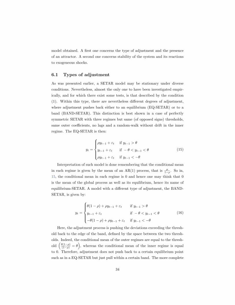
6.1 Types of adjustment

As was presented earlier, a SETAR model may be stationary under diverse

conditions. Nevertheless, almost the only one to have been investigated empir-

ically, and for which there exist some tests, is that described by the condition

(1). Within this type, there are nevertheless different degrees of adjustment,

where adjustment pushes back either to an equilibrium (EQ-SETAR) or to a

band (BAND-SETAR). This distinction is best shown in a case of perfectly

symmetric SETAR with three regimes but same (of opposed signs) thresholds,

same outer coefficients, no lags and a random-walk without drift in the inner

regime. The EQ-SETAR is then:

yt =

ρyt−1 + εt if yt−1 > θ

yt−1 + εt if − θ < yt−1 < θ

ρyt−1 + εt if yt−1 < −θ

(15)

Interpretation of such model is done remembering that the conditional mean

in each regime is given by the mean of an AR(1) process, that is µ1−ρ . So in,

15, the conditional mean in each regime is 0 and hence one may think that 0

is the mean of the global process as well as its equilibrium, hence its name of

equilibrium-SETAR. A model with a different type of adjustment, the BAND-

SETAR, is given by:

yt =

θ(1− ρ) + ρyt−1 + εt if yt−1 > θ

yt−1 + εt if − θ < yt−1 < θ

−θ(1− ρ) + ρyt−1 + εt if yt−1 < −θ

(16)

Here, the adjustment process is pushing the deviations exceeding the thresh-

old back to the edge of the band, defined by the space between the two thresh-

olds. Indeed, the conditional mean of the outer regimes are equal to the thresh-

old(θ(1−ρ)(1−ρ) = θ

), whereas the conditional mean of the inner regime is equal

to 0. Therefore, adjustment does not push back to a certain equilibrium point

such as in a EQ-SETAR but just pull within a certain band. The more complete

34

BAND-SETAR nests the EQ-SETAR so determining which model describe best

the data can be easily made.

Whereas the adjustment seems to be faster in a EQ-SETAR than in a BAND-

SETAR, it could be that a SETAR described by condition (4) (denoted by

returning-drift, RD-SETAR, by BF) has a faster adjustment. Effectively, the

outer regimes are unit root process with drift that may have much faster dy-

namics than simple AR processes. Despite of this potentially interesting feature,

RD-SETAR models don’t seem to have been used much in the literature, proba-

bly because of the unavailability of tests as we discussed below and also because

of the more complicated distribution of the parameters.

Note that the difficulty of the comparison of adjustment described by con-

ditions (1) to (4) comes partly from the fact that first the computation of the

mean of a SETAR model is difficult and requires numerical methods, and sec-

ond that the relevance itself of the concept of mean for non-linear model may

be questioned, due for example of the potential bimodality of the distribution of

the process. Concepts such as attractors and equilibria may be more adequate

(see Tong 1990), with the drawback nevertheless that those only be described

case to case. By extension, the term itself of mean-reversion in the SETAR

framework may be misleading. This is the case in the process 1 where mean-

reversion adjustment appears as a more restrictive condition than stationarity:

taking the case where µH > θH and µL < θLalong with |ρL| < 1 and |ρH | < 1

ensures stationarity but not mean-reversion to the inaction band: once in the

outer regime, the process may remain there.

Whereas the seminal paper of BF was based on models with three regimes (in

some cases the outer regimes are symmetric which may appear as a two-regime

specification), other studies (Enders and Granger 1998) focused on two-regimes

model. In our view, two-regimes models offer interesting insights into asymmet-

ric behaviors, though they have a complicated interpretation. Empirical studies

seek indeed to estimate a threshold in a two-regime model rather than imposing

its value to zero. Whereas in a three regime model it makes sense to observe

a strictly positive and a strictly negative threshold, there are few economical

arguments in favor of a two-regime model with a non-zero threshold, where

for example positive deviations would behave like small negative deviations but

differently from big ones.

35

6.2 Non linear impulse response functions

Note that the package tsDyn does NOT provide generalised impulse response

functions, altough it does provide standard imuplse response functions for the

linear VAR/VECM only, building on the function from package vars/urca. Sev-

eral people have been asking for this functionality, but it should not be too

difficult to do it with the existing functions, since tsDyn already implements

a TVECM.sim() and TVECM.boot() functions. For more informations, see

various discussions on the tsDyn mailing lists: http://groups.google.com/

group/tsdyn/t/5c517a94a3a3ab0c

7 Running the functions on parallel CPUs

A major drawback of the threshold cointegration tools is that those, due to the

probem of the unidentified parameter or the need of bootstrap replications, are

heavily computer intensive. The test of Seo (2006) takes indeed a very long time

to run.

To alleviate these problems, a possibility is to run the functions on parallel,

ie. either on a unique computer with multiple-CPUs processor or on more

complex computer clusters. Nowadays, it is quite common to find even laptops

equiped with processors like Intel Dual-Core, and hence parallel functionalities

can be used by practically everyone. Furthermore, it has become quite easy to

do it in R thanks to packages like foreach which offer a great level of abstraction,

requiring the user to do a minimal number of steps to get it running. Indeed,

this package will function as a wrapper for other parallel packages, and allows

the user to run it either on the protocol MPI, nws and pvm, or using the R internal

socket system, as well as the multicore22.

Furthermore, parallel computation is quite easy in the context of threshold

cointegration as the grid search or the bootstrap replications are independant

of each other and can easily be run on different nodes.

Parallel facilities are for now only available for the function TVECM.HStest(),

through the argument hpc (standing for high performance computing). When

22For a review on R facilities for high performance computing, see Schmidberger, Morgan,

Eddelbuettel, Yu, Tierney, and Mansmann (2009). There exist also a dedicated R mailing list,

as well as a task view http://stat.ethz.ch/CRAN/web/views/HighPerformanceComputing.

html

36

set to foreach, the package will run the foreach package. It is then up to the

user to choose a paralellisation protocol, the current choice being now between

doMC, doSNOW (MPI, pvm and nws, as well as internal R sockets), doMPI and

doRedis. We illustrate here with the easiest package, multicore, wich proved to

be quite powerful, with the disadvantage nerverthless that it can pose problems

when R is used within a GUI.

R codesystem.time(test1<-TVECM.HStest(dat, lag=1, nboot=200))

library(doMC)

registerDoMC(2) #Number of cores

system.time(test1<-TVECM.HStest(dat, lag=1, nboot=200, hpc="foreach"))

Results are quite impressive, as they show that by simply adding a second

core the execution time is divided by two, while using 4 cores will divide the

time by three, as shown in figure 323.

8 Conclusion

In this paper, I showed the interest of threshold cointegration towards tradi-

tional cointegration as being a better framework to model real world adjustment

process with stickiness and asymmetries. Indeed, a great number of empirical

studies applied this model, and an evenly great number of theoretical results

have been obtained. I presented also how one can use those developments using

the package tsDyn, offering a comprehensive framework for analysis and testing

that, despite of the great interest in this field, that was until now not available.

Using this package, one may conduce a whole analysis, testing for threshold

cointegration in different situations and different model specifications, and esti-

mating those models.

Whereas great developments occured since the seminal work in 1997, many

questions remain unanswered . The complexity of the SETAR model is actually

so high that simple aspects such its distribution or its moments are still only

known in restricted cases. Estimation of more than one threshold stills create

problems, and actual tests of stationary consider only a small amount of the

23It should be mentioned that the relationship between the number of CPUs and the reduc-

tion in execution time is decreasing with the number of CPUs: the more the CPUs, the less

their additional effect is.

37

Figure 3: Execution time of function TVECM.HStest using multiple cores

●

●

●

●

1 2 3 4

0.3

0.4

0.5

0.6

0.7

0.8

0.9

1.0

Number of procesors

Tim

e re

duct

ion

Number of bootstrap replications

n=1000n=500n=200

Running Hansen Seo test on multiple CPUs

38

possible features of a SETAR. There is up to now no framework allowing to test

the stationarity with an unknown cointegrating vector, and test discriminating

2 against 3 regimes only work in a restricted case.

References

Al-Abri, A. S., and B. K. Goodwin (2009): “Re-examining the exchange

rate pass-through into import prices using non-linear estimation techniques:

Threshold cointegration,” International Review of Economics & Finance,

18(1), 142–161.

Altissimo, F., and V. Corradi (2002): “Bounds for inference with nuisance

parameters present only under the alternative,” Econometrics Journal, 5(2),

494–519.

Andrews, D. W. K., and W. Ploberger (1994): “Optimal Tests When a

Nuisance Parameter Is Present Only under the Alternative,” Econometrica,

62(6), 1383–1414.

Balke, N. S., and T. B. Fomby (1997): “Threshold Cointegration,” Interna-

tional Economic Review, 38(3), 627–45.

Bec, F., A. Guay, and E. Guerre (2008): “Adaptive consistent unit-root

tests based on autoregressive threshold model,” Journal of Econometrics,

142(1), 94–133.

Bec, F., M. B. Salem, and M. Carrasco (2004): “Tests for Unit-Root versus

Threshold Specification With an Application to the Purchasing Power Parity

Relationship,” Journal of Business & Economic Statistics, 22, 382–395.

Chan, K., and H. Tong (1985): “On the use of the deterministic Lyapunov

function for the ergodicity of stochastic difference equations,” Advances in

applied probability, 17(3), 666–678.

(1990): “On Likelihood Ratio Tests for Threshold Autoregression,”

Journal of the Royal Statistical Society, 52(3), 469–476.

Chan, K. S. (1993): “Consistency and limiting distribution of the least squares

estimation of a threshold autoregressive model,” The Annals of Statistics, 21,

520–533.

39

Chan, K. S., J. Petruccelli, S. Woolford, and H. Tong (1985): “A

multiple threshold AR(1)model,” Journal of applied probability, 22(2), 267–

279.

Chan, K. S., and R. S. Tsay (1998): “Limiting properties of the least squares

estimator of a continuous threshold autoregressive model,” Biometrika, 85(2),

413–426.

Cheng, X., and P. C. B. Phillips (2009): “Semiparametric cointegrating

rank selection,” Econometrics Journal, 12(s1), S83–S104.

Damania, R., and B. Z. Yang (1998): “Price Rigidity and Asymmetric Price

Adjustment in a Repeated Oligopoly,” Journal of Institutional and Theoretical

Economics (JITE), 154(4), 659–.

Davies, R. (1977): “Hypothesis testing when a nuisance parameter is present

only under the alternative,” Biometrika, 64, 247–254.

(1987): “Hypothesis testing when a nuisance parameter is present only

under the alternative,” Biometrika, 74, 33–43.

de Jong, R. M. (2009): “Nonlinear time series models and weakly depen-

dent innovations,” Discussion paper, Department of Economics, Ohio State

University.

Dutta, S., M. Bergen, D. Levy, and R. Venable (1999): “Menu costs,

posted prices, and multiproduct retailers.,” Journal of Money, Credit, and

Banking, 31(4), 683–703.

Enders, W. (2001): “Improved Critical Values for the Enders-Granger Unit-

Root Test,” Applied Economics Letters, 8(4), 257–61.

(2004): Applied Econometric Time Series. Wiley, Hoboken, NJ, 2nd

ed edn.

Enders, W., and C. Granger (1998): “Unit-root tests and asymmetric ad-

justment with an example using the term structure of interest rates.,” Journal

of Business and Economic Statistics, 16(3), 304–311.

Enders, W., and P. L. Siklos (2001): “Cointegration and Threshold Adjust-

ment,” Journal of Business & Economic Statistics, 19(2), 166–76.

40

Engle, R. F., and C. Granger (1987): “Co-integration and error correction:

representation, estimation and testing.,” Econometrica, 55(2), 251–276.

Franses, P. H., and D. van Dijk (2000): Nonlinear Time Series Models in

Empirical Finance. Cambridge University Press.

Galvao, A. B. C. (2006): “Structural break threshold VARs for predicting US

recessions using the spread,”Journal of Applied Econometrics, 21(4), 463–487.

Gonzalo, J., and J. Pitarakis (2006a): “Threshold Effects in Multivariate

Error Correction Models,” in Palgrave Handbook of Econometrics, Volume

1: Econometric Theory, ed. by T. C. Mills, and K. Patterson, pp. 578–609.

Palgrave MacMillan.

Gonzalo, J., and J.-Y. Pitarakis (1998): “Specification via model selection

in vector error correction models,” Economics Letters, 60(3), 321–328.

(2002): “Estimation and model selection based inference in single and

multiple threshold models,” Journal of Econometrics, 110(2), 319 – 352.

(2006b): “Threshold Effects in Cointegrating Relationships,” Oxford

Bulletin of Economics and Statistics, 68(s1), 813–833.

Gonzalo, J., and M. Wolf (2005): “Subsampling inference in threshold au-

toregressive models,” Journal of Econometrics, 127(2), 201–224.

Gouveia, P., and P. Rodrigues (2004): “Threshold Cointegration and the

PPP Hypothesis,” Journal of Applied Statistics, 31(1), 115–127.

Granger, C., and P. Newbold (1974): “Spurious regressions in economet-

rics,” Journal of Econometrics, 2, 111–120.

Granger, C. W. J., and T. H. Lee (1989): “Investigation of Produc-

tion, Sales and Inventory Relationships Using Multicointegration and Non-

Symmetric Error Correction Models,” Journal of Applied Econometrics, 4,

145–159.

Gregory, A., and B. Hansen (1996): “Test for cointegration in models with

regime and trend shifts,” Oxford bulletin of economic and statistics, 58(3),

555–560.

41

Hansen, B. E. (1996): “Inference When a Nuisance Parameter Is Not Identified

under the Null Hypothesis,” Econometrica, 64(2), 413–30.

(1999): “Testing for Linearity,” Journal of economic Surveys, 13(5),

551–576.

(2000): “Sample Splitting and Threshold Estimation,” Econometrica,

68(3), 575–604.

Hansen, B. E., and B. Seo (2002): “Testing for two-regime threshold coin-

tegration in vector error-correction models,” Journal of Econometrics, 110,

293–318.

Heimonen, K. (2006): “Nonlinear adjustment in PPP evidence from threshold

cointegration,” Empirical Economics, 31(2), 479–495.

Horvath, M. T., and M. W. Watson (1995): “Testing for Cointegration

When Some of the Cointegrating Vectors are Prespecified,” Econometric The-

ory, 11(05), 984–1014.

Jawadi, F., N. Million, and M. E. H. Arouri (2009): “Stock market in-

tegration in the Latin American markets: further evidence from nonlinear

modeling,” Economics Bulletin, 29(1), 162–168.

Kapetanios, G., and Y. Shin (2006): “Unit root tests in three-regime SETAR

models,” Econometrics Journal, 9(2), 252–278.

Krishnakumar, J., and D. Neto (2009): “Estimation and Testing for the

Cointegration Rank in a Threshold Cointegrated System,” Discussion paper,

Working papers, Econoemtrics department University of Geneva.

Levy, D., M. Bergen, S. Dutta, and R. Venable (1997): “The Magnitude

of Menu Costs: Direct Evidence From Large U. S. Supermarket Chains,” The

Quarterly Journal of Economics, 112(3), 791–825.

Lo, M. C., and E. Zivot (2001): “Threshold Cointegration and Nonlinear

Adjustment to the Law of One Price,” M acroeconomic Dynamics, 5, 533–

576.

Lutkepohl, H. (2007): New Introduction to Multiple Time Series Analysis.

Springer, Berlin, corr. 2nd print edn.

42

Maki, D. (2009): “Tests for a Unit Root Using Three-Regime TAR Mod-

els: Power Comparison and Some Applications,” Econometric Reviews, 28(4),

335–363.

Million, N. (2004): “Central Bank’s interventions and the Fisher hypothesis: a

threshold cointegration investigation,”Economic Modelling, 21(6), 1051–1064.

Nelson, and Plosser (1982): “Trends and Random Walks in Macroeconomic

Time Series: Some Evidence and Implications.,” Journal of Monetary Eco-

nomics., 10(2), 139–162.

Perron, P. (1989): “The Great Crash, the Oil Price Shock, and the Unit Root

Hypothesis,” Econometrica, 57(6), 1361–1401.

Petrucelli, J., and N. Davies (1986): “A portmanteau test for self-exciting

threshold autoregressive-type nonlinearity in time series,” Biometrika, 73(3),

687–694.

Pfaff, B. (2008a): Analysis of Integrated and Cointegrated Time Series with

R. Springer, New York, second edn., ISBN 0-387-27960-1.

(2008b): “VAR, SVAR and SVEC Models: Implementation Within R

Package vars,” Journal of Statistical Software, 27(4).

Phillips, P. (1986): “Understanding spurious regressions in econometrics,”

Journal of Econometrics, 33(3), 311–340.

Phillips, P., and S. Ouliaris (1990): “Asymptotic Properties of Residual

Based Tests for Cointegration,” Econometrica, 58(1), 165–193.

Pippenger, M. K., and G. E. Goering (2000): “Additional Results on the

Power of Unit Root and Cointegration Tests under Threshold Processes,”

Applied Economics Letters, 7(10), 641–44.

Samuelson, P. (1965): “Proof That Properly Anticipated Prices Fluctuate

Randomly,” Industrial Management Review, 6, 41–49.

Schmidberger, M., M. Morgan, D. Eddelbuettel, H. Yu, L. Tierney,

and U. Mansmann (2009): “State of the Art in Parallel Computing with R,”

Journal of Statistical Software, 31(1), 1–27.

43

Seo, M. (2006): “Bootstrap testing for the null of no cointegration in a threshold

vector error correction model,” Journal of Econometrics, 127(1), 129–150.

(2008): “Unit Root Test In A Threshold Autoregression: Asymptotic

Theory And Residual-Based Block Bootstrap,” Econometric Theory, 24(06),

1699–1716.

(2009): “Estimation of non linear error-correction models,” Discussion

paper, London School of Economics, Consulted in July 2009.

Seo, M., and O. Linton (2007): “A smoothed least squares estimator for

threshold regression models,” Journal of Econometrics, 141(2), 704–735.

Sims, C. A. (1980): “Macroeconomics and Reality,” Econometrica, 48(1), 1–48.

Stock, J. H. (1987): “Asymptotic Properties of Least Squares Estimators of

Cointegrating Vectors,” Econometrica, 55:5, 1035–1056.

Taylor, A. M. (2001): “Potential Pitfalls for the Purchasing-Power-Parity

Puzzle? Sampling and Specification Biases in Mean-Reversion Tests of the

Law of One Price,” Econometrica, 69(2), 473–498.

Tong, H. (1990): Non-Linear Time Series. A Dynamical System Approach.

Oxford Science Publications.

Tsay, R. S. (1989): “Testing and Modeling Threshold Autoregressive Pro-

cesses,” Journal of the American Statistical Association, 84(405), 231–240.

Ward, R. (1982): “Asymmetry in Retail, Wholesale and Shipping Point Pricing

for fresh Vegetables,” American Journal of Agricultural Economics, 64(2),

205–212.

Zivot, E., and D. W. Andrews (1992): “Further Evidence on the Great

Crash, the Oil-Price Shock, and the Unit-Root Hypothesis,” Journal of Busi-

ness & Economic Statistics, 10(3), 251–270.

44