power and irrigation subsidies in andhra pradesh & …pdf.usaid.gov/pdf_docs/pnadk228.pdf1 power...
TRANSCRIPT

Power and Irrigation Subsidies in Andhra Pradesh & Punjab
Shyamal Chowdhury Maximo Torero
March 2007
International Food Policy Research Institute
Washington, D.C.
Contact Person at IFPRI Maximo Torero, Director, MTID, IFPRI, Washington D.C.
Email: �[email protected]


1
Power and Irrigation Subsidies in Andhra Pradesh & Punjab
Executive Summary
o It is generally agreed that the use of electricity in agriculture for irrigation following the green revolution has significantly contributed to agricultural productivity growth in India. However, there is an inbuilt inefficiency in the current pricing mechanism and measuring system, and allocation of subsidy on electricity for irrigation. This report examines the general setting of the subsidy on electricity for irrigation and proposes an alternative institutional mechanism to minimize the inbuilt inefficiency in the current pricing mechanism so to assign the subsidy in a more efficient way.
o In AP and Punjab, the cost of electricity for irrigation for majority of the farmers is fixed per month since they pay a monthly fee based on pump capacity (Horse Power). It implies that at the margin, farmers incur almost a zero cost for irrigation in the short-run (ignoring depreciation cost due to additional use and marginal labor cost of additional use). Given that the marginal cost of other inputs required in agriculture production are not zero and assuming that the production technology that farmers use ensure positive marginal return to input substitution, farmers have a pervasive incentive to overuse electricity for irrigation. Similar to input substitution, farmers have incentives for production substitution and extend production to more water intensive crops. This is what has exactly happened: since fifties there is a significant shift of production patterns towards rice and wheat which are more water intensive in nature.
o The major consequences of the current pricing mechanism and subsidy scheme
are: o Jump in electric pump use - A significant increase in use of electric pump for
irrigation and in the electricity consumption per pump set. [Some numbers] o Jump in the share of electricity consumption in agriculture - The share of the
electricity consumption by agriculture with respect to domestic, industry and commercial, had increased from 3.9% in 1960, to 10% in 1970, to 18% in 1980 and to 32.2% in 1998.
o Huge deficit with respect to revenue – Even though the share of agriculture in electricity consumption increased many folds, the share of agriculture in the revenue had essentially remained the same resulting in a significant deficit and therefore a significant increase in the subsidy.
o Reduction of cross-subsidy – reforms has not been yet successful and costs of supply have been going up reducing the possibility of cross-subsidization of agriculture from other sectors such as industry and commerce.
o Subsidy substantially increased - The subsidy had increase from Rs 155.9 billion in 1996-97 to 281.2 billion in 2001-2002. Specifically, in Andhra Pradesh it had increased from 7.3 billion in 1991-92 to 41.8 billion in 2001-2002; and from 6.9 billion to 23.4 billion in Punjab.

2
o Deterioration of supply – there is a significant deterioration of the quality of the supply and also a significant increase in the losses in transmission and distribution. This is a consequence of the inadequate expenditure in maintenance and inadequate investment in transmission and distribution lines
o Environmental damage – the ground water level has fallen substantially. In the case of Andhra Pradesh all the blocks has experienced a fall on the ground water level bigger than 4 meters since 1984. There has been an annual fall of 20cms per year. In the case of Punjab 4/5 of the blocks are also under four meters since 1984, 52.17% of the total blocks in the state are over-exploited and 7.97% of all blocks are ‘dark’ areas as on 31-3-98 (GOI, 2002b) and are also considered over exploited, i.e. the net recharge is substantially negative. The over-exploitation of underground water has caused a fall in the water table in large parts of the state and this has entailed increased expenditure on deepening of tube wells.
o Subsidy is regressive – The beneficiaries of the subsidy are clearly the richest households. For example, although small and marginal farmers constitute the majority of electric pump set owners in AP, medium and large farmers receive a disproportionately large share of the total agricultural power subsidy (68%, i.e. they operate 68% of the area irrigated by electric pump sets). Approximately 39% of the subsidies accrue to large farmers who represent 15% of electric pump set owners and less than 2% of all rural households. Marginal farmers, who represent 39% of all electric pump owners, receive 15% of the subsidy (World Bank 2003). Similar results can be found in Punjab.
o Linked to the pricing mechanism is the measurement problem that breeds
inefficiency and corruption. At present, there is no accurate estimate of actual power consumption in agriculture. Currently it is measured as a residual consumption after deducting non-agricultural consumption, and technical losses from total production. If actual consumption is known, public authorities can decide on financing needs and financing methods. Studies that measured actual consumption came up with estimates much lower than the official consumption figures. For instance, World Bank (2001) that put meter at pump level to study the actual use of electricity in Haryana found that the degree of over-estimation of un-metered consumption ranges from 49% to 154%.
o From the above results it is clear that there is a need to identify alternative institutional mechanisms to reduce inefficiency in assigning the subsidy, and to gradually reduce the subsidy to improve quality and quantity of power and to reduce the growing trend of environmental damage.
o This research report proposes a strategy of price discrimination based on the size of the farmers plot and on the implementation of a two part tariff mechanism. Specifically three types of consumers are identified, small holders (more than zero ha and less or equal to 1.8 ha), medium holders (more than 1.8 ha and less or equal than 3.64 ha) and large holders (more than 3.64 ha) and a common two part tariff is proposed. The advantage of this two part tariff is that the first part of the tariff will be equivalent to the value of the average current consumption of the

3
small holders, which will, at the same time, be the amount of the subsidy. This will assure that on the one hand, the small holders will on average not be affected by this new price mechanism, and on the other hand, the subsidy will be better targeted. The second part of the tariff will be set at levels higher than the marginal cost in such a way that high demanders will cover their costs and if possible cross subsidize the small holders.
o The simulations of demand under the implementation of the proposed two part
tariff involved two different data sets. The first data set is the 54th Round of the National Sample Survey (NSS). This data set provided us with accurate information on the lands owned by farmers in Andhra Pradesh and Punjab. The second database was the 55th Round of the NSS which included information on household consumption of electricity for these regions and therefore allow us to estimate the demand elasticities necessary to measure the impact of changes in the pricing policies.
o Elasticities where estimated based on the almost ideal demand system (AIDS)
initially developed in Deaton and Muellbauer (1980) and later on improved by other authors. The own price eleasticity for Andhra Pradesh and Punjab together is -0.5192, and the price eleasticity for each of the consumer groups based on the size of their land possession can be summarized in:
Own Price Elasticities of power consumption
Andrah Pradesh PunjabAll -0.67 -0.85Marginal/ Small holders -0.69 -0.91Medium holder -0.55 -0.91Large holders -0.50 -0.86
In addition, we review previous work on estimation of price elasticities for electricity for agriculture and we found evidence that our estimates were close to previous efforts. Specifically, Bose and Shukla; (1999), estimated, based on time series data for 9 years (from 1985/86 to 1993/94) pooled over 19 Indian States (which includes Punjab and Andhra Pradesh), price elasticities for the agriculture sector of -1.35.
o Based on the above elasticities and the one of Bose and Shukla (1999) we have simulated the impact of three progressive pricing schemes.
o The first price scheme is a simple two part payment schedule that established an initial quantity (q1) priced at p1; while demand exceeding q1 units is priced with marginal cost, i.e. p2. This scheme is conceived with two conditions. Firstly, expenditure of smallholders should not be affected by changes in the price scheme, so that the smallholders will continue to receive the current subsidy and therefore, their consumption of electricity for irrigation will remain unchanged, and secondly that this subsidy will also be present on the medium and large holders but only up to the amount

4
of average consumed kwh by smallholders, in additional quantity used will be charged at the marginal cost. To be able to implement this, p1 and q1 were established as the average quantity and price in the electricity demand of smallholders. Consumption exceeding q1 in the other two categories (medium and large holders) is priced at the marginal cost p2. The main results can be summarized as follows: In the case of Andhra Pradesh small holders continue to consuming the same amount of electricity at the same price; medium holders reduce their consumption by 14% and their weighted price (combinations of the first and second part of the tariff weighted by the quantity consumed in each part) increases by 25.1%; and finally, large holders reduce their consumption by 41% and their weighted price increases by 82.2%. In the case of Punjab small holders continue to consuming the same amount of electricity at the same price; medium holders reduce their consumption by 16% and their weighted price increases by 17.1%; and finally, large holders reduce their consumption by 47% and their weighted price increases by 55.3%. This new price schedule assures that the subsidy is distributed in a more progressive way.
o The second price scheme is designed to significantly improve the progressiveness of the distribution of the subsidy with respect to the first two part tariff mechanism. In addition, this new pricing mechanism has the objective to reduce (not to eliminate) the burden of the subsidy to the government by cross subsidizing small holders with the revenues from large holders. This second mechanism considers a fixed rate (F), under which the household receives q1 units of electricity. Consumption exceeding q1 is charged with a marginal cost v1 for households demanding less than q2 units, and households with consumption exceeding q2 will pay v2 for additional units. Similarly, and with the same logic of the first tariff scheme, the fix rate (F) is calculated as the average consumption and expenditure of small holders so that they will not be affected by this new price scheme. In the case of Andhra Pradesh with tariffs of v1=2 ruppies per kwh and v2=3.45 ruppies per kwh the subsidy can be reduced to 33% of the current subsidy and large holders will cross subsidize small holders reducing significantly the burden of the government. In the case of Punjab the prices of v1 and v2 will have to be 4.9 and 5 to be able to arrive to a similar scenario as Andhra Pradesh. This is so because the land ownership is far more concentrated in Punjab than in Andhra Pradesh and therefore under the current situation the subsidies are clearly benefiting a lot more the large holders. In addition, we have simulated the impacts under different scenarios of marginal costs.
o Finally, the third pricing mechanism has as objective to move a step forward from the second price mechanism and to completely eliminate the burden of the subsidy to the government. To be able to implement this mechanism, not only a new simulation introducing variable parameters (v1 and v2) as in the previous tariff schedule is kept, but also raises of the fixed rate are introduced. While increases in fixed rates may allow for

5
reductions in the electricity subsidy, it may also reduce the subsidy for the small holders (i.e. 66% and 44% in Andhra Pradesh and Punjab, respectively). As expected the higher the level of the first part of the tariff the more the small holders will pay for the service and therefore the smaller the level of the subsidy for the first part of the tariff.
o In summary, in all these three price schemes, the major result is that the subsidy
will be more progressive and resources will be used more efficiently. If low-demand consumers or high-demand consumers want to consume more electricity, they will need to pay a charge over the marginal costs for each unit above their fixed charge.
o Although any of these price schemes can be implemented based on existing
information, the ideal situation would be, and specially to be able to move to gradual elimination of the subsidies (i.e. from price scheme 1 to scheme 3), there is a clear need to develop better mechanisms to measure consumption and consumption patterns of households. With this respect the use of pre-paid meters will be an ideal solution to better implement the alternative pricing mechanisms. The identification of farmers will allow to a better allocation of subsidies on poorer farmers. The resources for this subsidy should not be higher than the total amount that can be collected from other consumer groups.
o Punjab and Andhra Pradesh are currently in a critical and unsustainable situation
as the ground water level has fallen substantially. These price schemes will contribute significantly in the reduction of the over consumption of power and therefore of underground water as farmers will now have to pay at least the marginal cost for the electricity they use. At the same time with the reduction of total subsidy, the government should be able to increase investment in the power sector to improve quality and quantity supplied as well as to increase their efficiency reducing transmission and distribution losses and improving the quality of the service. In conclusion, these recommendations could open an alternative to move from a vicious circle, in which the environmental situation will substantially worsen and the capacity of generation of electricity will be seriously damaged, to a virtuous circle, where the subsidy is assigned in a more progressive way, the trend in reduction of underground water is overturned and the electric providers can have sufficient resources to improve the quality of the electricity supplied.

6
Index �HChapter 1: Introduction....................................................................................................... ��H7 �HChapter 2: Power for Irrigation, Power Sector Reform and Canal Irrigation................... ��H12
�H2.1 Introduction............................................................................................................. ��H13 �H2.2 Reform and Restructuring in Power Sectors .......................................................... ��H16
�HChronology of Reforms ............................................................................................ ��H16 �HCauses of Reforms and Consequences ..................................................................... ��H17 �HOrganization and regulatory structure of power sector in India ............................... ��H18
�H2.3 Vicious Cycle of Power Supply in Agriculture ...................................................... ��H19 �H2.3.1 Rising demand for power in agriculture .......................................................... ��H21 ��H2.3.2 Growing imbalances in revenue, cost and tariff .............................................. ��H23 ��H2.3.3 SEBs’ low supply ability ................................................................................. ��H25 ��H2.3.4 Supply outcomes.............................................................................................. ��H26
��H2.4 The State of Canal Irrigation .................................................................................. ��H27 ��H2.4.1 Canal Networks and Subsidies ............................................................................ ��H29 ��H2.4.2. Reforms in Canal Irrigation................................................................................ ��H29 ��H2.5 Who are the beneficiaries of irrigation subsidy? .................................................... ��H30
��HChapter 3: Rural Households Demand for Electricity...................................................... ��H34
��H3.1 Introduction ............................................................................................................ ��H34 ��H3.2. The AIDS model.................................................................................................... ��H34 ��H3.3 Data......................................................................................................................... ��H35 ��H3.4 Results .................................................................................................................... ��H37
��HChapter 4: Rural Households Demand for Electricity...................................................... ��H41
��H5.1 Introduction ............................................................................................................ ��H41 ��H4.2 Price discrimination and two part tariffs ................................................................ ��H42 ��H4.3 Simulating impacts of a two part tariff – Simulation 1 .......................................... ��H44 ��H4.4 Simulating impacts of an optimal consumption plan with a fix rate and two variable marginal rates – Simulation 2 ......................................................................... ��H50 ��H4.5 Simulating impacts of an optimal consumption plan with a variable fix rate and two variable marginal rates – Simulation 3 .................................................................. ��H68 ��H4.6. Metering as a Necessary Condition and the alternative of Pre-paid Meters ......... ��H71
��H5. Conclusions .................................................................................................................. ��H72 ��HReferences ........................................................................................................................ ��H76 ��HAppendix .......................................................................................................................... ��H79

7
Chapter 1: Introduction The questions of how to reduce the current subsidy given in electricity for irrigation in agriculture in India, and what are the alternative institutional mechanisms to allocate such subsidies in an equitable way are some basic concerns for policy makers and development thinkers during recent times. In this study, these two questions are dealt with in the specific context of two Indian States – Andhra Pradesh (henceforth, AP) and Punjab. The study examines the general setting of the subsidy on electricity for irrigation in these two states, and proposes few alternative solutions to choose from that can reduce the subsidy burden on state government and increase efficiency, and yet keeps the benefits for small farmers unchanged, therefore ensuring equity. The role of irrigation in agricultural productivity growth following green revolution in India and as well as in other South Asian countries is well recognized (e.g., Larson et al 2004, Smith 2004). Subsidy in electricity for irrigation in agriculture worked as a strong incentive for farmers – both large and small – to buy electric pump, to use irrigation, and to shift production to irrigated crops. Partly due to rapid growth in irrigation owing to subsidized electricity, the total food grain production in India increased by more than two-folds in less than forty years between 1960 and 2000. Two states that played important roles in this increased production are AP and Punjab. Coincidently, these are the two states that highly subsidize electricity for irrigation and are facing the curse of unsustainable budget deficit, low-quality in power supply, over-exploitation of ground water, and environmental degradation. AP is considered as the “Rice Bowl” of South India and contributes a major share of food grains to the central pool. Total food grain production in 2000-01in AP was 15.04 million metric tons. In its vision 2020, AP sets an impressive target of growing at a rate of above 10 percent per annum for a period of 25 years starting from 1995 (Vision 2020). However, the current growth rate is well below the targeted one. Figure A1.1 in Appendix shows the basic indicators of AP. It is the 5th largest state in India in terms of geographical area (275045 sq km, 8.97% of geographic area) and population size (75.73 million in 2001, constituting 7.37% of India’s total population). Punjab is the chief granary of India contributing 6.79 million metric tons (42.1%) of rice and 7.83 million metric tons of wheat (55.4%) to the Central pool in 1999-2000 (http://www.punjabenvironment.com/status.htm). However, agriculture relies heavily on irrigation due to the climatic conditions.�F
1 Figure A1.2 in Appendix shows the basic indicators of Punjab. During recent years, the overall economic performance of Punjab was below the all-India average. In 2001-02, agriculture (including allied sectors) grew at a rate of 0.76% and GSDP grew at a rate of 3.47%. During this 1 Punjab has a subtropical climate with hot summers and cold winters. The annual rainfall is around 532 mm in plains and 890 mm in the northern sub-mountain regions. However, 70% of the annual rainfall is received during monsoon months. Therefore, agriculture depends mostly on irrigation (Punjab Environment).

8
period, the revenue deficit, and total debt as a percentage of GSDP reached to 5.28% and 45.35%, respectively (Budget Speech for the year 2003-04). While agriculture is the mainstay of Punjab economy, it is based on paddy-wheat rotation. Though this overspecialization worked well during the green revolution, the productivity of both the crops has almost stagnated at present. Growing budget deficit and mounting debt largely due to subsidy, and a stagnant agriculture are attributable to the poor performance of the state economy.
Table 1: Irrigated Area, Irrigation Sources, and Production in AP and PJ in 1 960 and 2001
Total Net Area under~ Area Under Production of Irrigated Area Canal TW Rice Food Grains Rice Food Grains
AP 1961-62 30.29/a 12.66/a 0.2/a 29.61/a 91.43/a 3.661/a 6.421/a 2000-01 45.28/b 16.49/b 10.66/b 42.43/b 76.73/b 12.458/b 15.04/b
PJ 1960-61 20.20/c 11.80/c 8.29/c 2.29/b 30.63/e,f 0.229/b 3.162/e,f 1970-71 28.88/b 12.92/b 15.91/b,d 3.9/b 39.27/b 0.688/b 7.305/b 2000-01 40.21/b 10.02/b 30.17/b,d 26.12/b 61.55/e.f 9.157/b 24.898/e,f
AI 1960-61 246.61/b 103.70/b 1.35/b 341.3/b 1155.58/b 34.58/b 82.02/b 2000-01 546.82/b 159.89/b 217.24/b 446.2/b 1210.5/b 84.98/b 196.81/b
Notes: AP: Andhra Pradesh, PJ: Punjab, AI: All India; ~ total irrigated area is greater than the combined area under canal and tube well due to other sources of irrigation; Areas are in ’00,000’ hectares, and production in`000,000' tons; Food grains include all cereals and all pulses. TW: Tube Well. Tanks, other wells except TW and other sources are not shown in the Table 1. Sources: a/ Directorate of Economics and Statistics, Andhra Pradesh, http://www.ap.gov.in/apbudget b/ Indiastat.com c/ Hira and Khera 2000 d/ Wells and tube wells together e/ 2001-02 f/ http://www.punjabgov.net/about_agri2.asp Table 1 shows major changes in total net irrigated area (in ‘00000’ hectares), area under canal irrigation and tube-well (TW) irrigation, area under rice and food grain production, and total production of rice and food grains in Andhra Pradesh (AP) Punjab (PJ) and All India (AI). Two major developments in agriculture and food sector in India in general and in AP and Punjab in particular since 1960s are: first, increase in food grain production; and second, increase in area under irrigation. In AP in particular and also in Punjab, the net area sown has remained stable during the last four decades (Table A2a, A2b in Appendix). However, despite this, the total food grain production in AP has increased from 6.4 million metric tons in 1960-61 to 15.04 million metric tons in 2000-01. Food production in Punjab has shown even more dramatic increase, from 3.1 million metric tons in 1960-61 to 24.9 million metric tons in 2001-02. Therefore, the additional food produced there during the last three decades came primarily from increased productivity in food production. Highly linked to the increased food production is the increased availability of irrigation in AP and Punjab. In AP, the total net irrigated area as a percentage of total net sown area increased from 26.98% in 1960-61 to 39.07 in 1990-91. In Punjab, it increased from 53.77% in 1960-61 to 94.95% in 1997-98 (Table A1a, A1b in Appendix). Therefore, expansion in irrigation acted as one of major forces in the

9
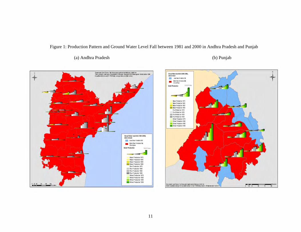
increased food production. In fact, a simple comparison between irrigated and non-irrigated plots shows a significant productivity differential that persists over time (Table A1e in Appendix). Though the productivity differences observed between irrigated and non-irrigated fields are not entirely due to irrigation, persistence of productivity differential across time and across crops indicates that productivity differential may be partly explained by irrigation differential. Looking at the cropping pattern, the availability of irrigation has resulted in a cropping pattern that is highly irrigation-intensive. This is due to the pervasive incentives given to farmers in irrigation in the form of subsidized electricity for irrigation. Out of 5.158 million hectares gross irrigated area in AP during 1997-98, paddy alone covered 3.373 million hectares (65.45%). In Punjab, area under paddy production as a percentage of total cropped area increased from 4.8% in 1960-61 to 31.3% in 2001-02. Two crops, rice and wheat together, had a command area of around three-quarters of the total cropped area in the state in 2001-02 (Table A1c and Table A1d in Appendix). Needless to say that these are the two very water-intensive crops that are replacing many other low water-intensive crops. Coupled with high budget deficit and the spread of water-intensive crops comes the overexploitation of water and environmental degradation. In Punjab, 77% area of the state is facing a problem of falling water table. Most of these areas fall in the central part of the state that produces about 67% of rice and 56% of wheat (Hira and Khera 2000). Overexploitation of ground water is evident in AP too. In 1999-2000, the number of dark mandals�F
2 was around 45% of total mandals, and 92% of the areas reported falling in ground water (Reddy 2003). Figures 1a and 1b link the production pattern and ground water level fall between 1981 and 2000 in AP and PJ. Both in AP and PJ, the fall in ground water and the irrigation-intensive production pattern seem highly correlated. Between the two sources of irrigation subsidies in agriculture – electricity and canal – the main focus of the current study is on the subsidy on electricity for irrigation, and not on the subsidy on canal irrigation for two reasons: first, changes in irrigation during recent time are due mostly to tube-well most of which are electric tube wells (Table 1). As we will see in the brief review of canal irrigation in Chapter 2, the share of total irrigated area under canal irrigation had in fact declined in recent times. Second, canal irrigation does not create negative externalities apart from distortions created by subsidy. In fact, unlike electricity based ground water irrigation, canal irrigation helps to arrest the fall of ground water level therefore create positive complementarities. Therefore, full cost pricing of canal water based irrigation may not be justified. However, it should be mentioned that the mechanisms suggested here can be applied, with appropriate modifications, to canal irrigation subsidy as well. Previous works on how to reduce the subsidy and what kind of mechanisms are needed to reduce subsidies focus mostly on supply side management. As we will see in our brief review of the current state of power supply to agriculture, there are 2 Mandal is the lowest administrative unit in AP comprising of several villages.

10
important supply side issues, e.g., quality of electricity, corruptions, etc, that need to be taken care of. And the existing literature has pointed out these very vividly. However, the problem with such recommendations is that improving supply without managing demand will misalign the incentive structure further and may aggravate the overall scenario.
11
Figure 1: Production Pattern and Ground Water Level Fall between 1981 and 2000 in Andhra Pradesh and Punjab
(a) Andhra Pradesh (b) Punjab

12
In this study, we rely on demand management and propose three alternative pricing schemes based on a two-part tariff mechanism. The proposed schemes are based on farmers’ plot size that are easy to observe, and can be implemented with little or less new information. All of the pricing schemes proposed here are equitable in nature and can keep the benefits of existing subsidy for any particular group, such as small farmers, unchanged. Such a scheme can also reduce the overall subsidy burden on states, send the correct signal to farmers thereby disciplining them on water-use, and shifting them to crops diversification, and arrest the environmental damage caused by over-exploitation of ground water. The rest of the study proceeds as follows: Chapter 2 provides a brief overview on the electricity for irrigation, the current reforms in power sector, and outcomes. It also gives a brief overview of the state of canal irrigation as a complement to power irrigation. It then links the current subsidy scheme that has created a vicious cycle of rising demand, growing imbalances, low supply ability and poor supply outcomes. Based on this section, the study looks at the current distribution of irrigation subsidy and identifies the beneficiaries of subsidies based on household level information. Chapter 3 estimates the demand for electricity and calculates the price and other elasticies that are used in Chapter 4. Chapter 4 proposes alternative pricing schemes and simulates them based on elasticities derived in Chapter 3. It also shows how these proposed pricing schemes can be used to turn the vicious cycle into a virtuous cycle. Chapter 6 concludes with policy recommendations.

13
Chapter 2: Power for Irrigation, Power Sector Reform and Canal Irrigation 2.1 Introduction It is generally agreed that the use of electricity in agriculture (irrigation) following the green revolution has significantly contributed to agricultural productivity growth in India (e.g., Larson et al 2004, Smith 2004). Figure A2.1a in Appendix plots the production of food grains against the use of electricity in agriculture supporting this view. While in 1950, the use of electricity in agriculture was 2 Kwh per hectare, it increased to 7 Kwh per hectare in 1960 and to 36 Kwh per hectare in 1970. During this period, the corresponding figures for food grains production per hectare were 522 Kg, 710 Kg, and 872 Kg. Therefore, a strong association exists between the use of electricity in agriculture and the productivity in agriculture and the correlation coefficient between these two is 0.94. However, despite this strong association, the use of electricity in agriculture has already shown the sign of diminishing marginal return starting from 80s as can be seen in Figure A2.1a. Canal water is also an important source for irrigation although changes in irrigation during recent time are due mostly to tube-well most of which are electric tube wells (as can be seen in figures 2.1a, b and c.) and the share of total irrigated area under canal irrigation had in fact declined in recent times.
Figure 2.1a
Irrigated Area (in lakh ha) and Sources in AI
247
104
1
547
160217
0
100
200
300
400
500
600
Total Canal TW
1961-62 2000-01

14
Figure 2.1.b Irrigated Area (in lakh ha) and Sources in AP
30
13
0.2
45
1611
05
101520253035404550
Total Canal TW
1961-62 2000-01
Figure 2.1.c
Irrigated Area (in lakh ha) and Sources in PJ
29
1316
40
10
30
05
1015202530354045
Total Canal TW
1970-71 2000-01 Consumption of electricity is synonymous to the use of electricity in ground water irrigation and in this study we will use these two terms, use of electricity in agriculture and in irrigation interchangeably. The importance of power in groundwater irrigation cannot be exaggerated. In AP in 2001-02, well covered more than 45% of net irrigated area and in Punjab in 1997-98, well covered around 60% of net irrigated area. As we will see latter in the chapter that due to the electrification of pumps, the role of diesel pumps have been largely replaced, and it is largely the electric pump that has emerged as the major means of irrigation. As of March 2002, the total number of electric pump in AP and Punjab reached to 1934389 and 811252, respectively (GOI 2002a). These represented 98% achievements of electrification potential for AP and above 100% for Punjab. However, there is a strong mismatch between consumption share and revenue share. Despite this increased share of agriculture in electricity consumption, the relative contribution of agriculture in total revenue from electricity sale has not increased and has remained around 5% or less in 1990s (sees Figure A2.1b in Appendix). Though there
15
were improvements in few states after the initiation of power sector reforms in the late 90s, the overall scenario has remained relatively unchanged. Especially, states with a very high share of agriculture in total electricity consumption, such as AP and Punjab, have not shown any improvement in additional revenue generation from agriculture. This has created imbalances that are threatening the power sector and spilling over to other sectors. There is an inbuilt inefficiency in the current pricing mechanism and measuring system of power for irrigation. In AP and in many other states in India, the cost of electricity for irrigation for majority of the farmers is fixed per month since they pay a monthly fee based on pump capacity (Horse Power). It implies that at the margin, farmers incur almost a zero cost for irrigation in the short-run (ignoring depreciation cost due to additional use and marginal labor cost of additional use). Given that the marginal cost of other inputs required in agriculture production are not zero and assuming that the production technology that farmers use ensure positive marginal return to input substitution, farmers have a pervasive incentive to overuse electricity and water.�F
3 Looking at the average electricity use per pump in Punjab where electricity for irrigation is free, and the rapid depletion of ground water table there, the overuse of electricity and water becomes evident (Figure A2.1c in Appendix). Linked to the pricing mechanism is the measurement problem that breeds inefficiency and corruption. In fact, in some sense, the current problem of tariff rationalization in agriculture is basically a measurement problem. At present, there is no accurate estimate of actual power consumption in agriculture. Currently it is measured as a residual consumption after deducting non-agricultural consumption, and technical losses from total production. However, the current measurement has in-built incentives for corruption and by passing technical losses, inefficiencies, and consumption in other sectors under the name of agricultural consumption. If actual consumption is known, public authorities can decide on financing needs and financing methods. Studies that measured actual consumption came up with estimates much lower than consumption figures suggested by state electricity boards. For instance, World Bank (2001) that put meter at pump level to study the actual use of electricity in Haryana found that the degree of over-estimation of un-metered consumption ranges from 49% to 154%. Provision of electricity and irrigation at concessions has encouraged inefficient use of a scarce resource such as water, distorted the inter-temporal resource allocation, and promoted spatial, inter-personal and inter-temporal inequities. In Punjab, 52.17% of the total blocks in the state are over-exploited and 7.97% of all blocks are ‘dark’ areas as on 31-3-98 (GOI 2002b).�F
4 The over-exploitation of underground water has caused a fall in the water table in large parts of the state and this has entailed increased expenditure on deepening of tube wells (see Map 1b). In case of canal irrigation, it is found that 44 percent of the water entering the canal got lost in the canal itself, 27 percent of the water is wasted by the farmers through excessive use and only 29 percent is actually used by
3 For instance, Gulati (1999) mentioned that farmers in India use irrigation water for controlling weed growth – an example of input substitution created by falls incentives. 4 The ‘dark’ areas are those blocks where ground water use is more than 85% of the utilizable recharge.
16
the crops (Veeraiah and Madankumar, 1994). In case of spatial inequality, one of the common complaints of farmers is that the tail-ender does not get adequate supply of irrigation water due to overdraw by those located at the head-reach. 2.2 Reform and Restructuring in Power Sectors India followed a gradual approach in its power sector reform. During the pre-reform period that is prior to 1991, the State Electricity Boards (SEBs) were responsible for power supply. They were vertically integrated monopolies that controlled around 70% of gross generation�F
5, most of the intra state transmission, and almost all of the distribution. Though SEBs were statutorily required to function as autonomous service-cum-commercial entities, the commercial requirement was largely ignored and service provision was grossly misaligned from social objective as well (World Bank 2001).
Chronology of Reforms ��H Table A2.2a in Appendix shows the chronology of power sector reform in India. The country started with opening up of its power generation to private sector in 1991 without making any change in market or regulatory structure of electricity industry. It was the easiest reform to implement since SEBs were buying power prior to reform. However, the reform had limited success since it did not add sufficient generation capacity. One of the prime reasons for which reforms failed to attract private investment in generations was the weak financial health of SEBs. Private investors and lenders were worried of supporting projects that had to rely on the purchasing capacity of almost bankrupt monopsonies (IDFC 1998). Failing to head up with a partial reform program, the government embarked on a larger reform agenda in the mid 90s. This second wave of reform came into force in 1996 when the Common Minimum Action Plan for Power (CMNAPP) was framed. That led to three major changes in market and regulatory structure and pricing. The changes are: First, setting up of independent regulatory commissions at the union and state level; second, restructuring and corporatizeing of SEBs; and third, rationalization of tariffs (see Figure A2.2a in Appendix). Setting up of independent regulatory commissions at state level achieved considerable success and by 2003, most of the states had their state electricity regulatory commissions (SERCs) and published their first tariff order (GOI 2002a). This was an important step towards separating tariff-settings from operations. It is expected that due to this separation, regulatory commissions, being independent from the government, would be able to rationalize tariffs, which is normally a politically sensitive and unpalatable decision for the governments. SERCs are reasonably independent in setting tariffs though their competence and composition are not without questioned.�F
6 5 The exact share of SEBs in gross electricity generation excluding EDs in 1992-93 was 68.28% or 205550 MKwh. Source: GOI 2002a, p.58. 6 Our own experiences in dealing with regulatory commissions in AP and PJ are far from satisfactory.
17
Though there could be minor variations, the restructuring of SEBs in India has followed a general pattern of unbundling into a single generation company (GenCo), a single transmission company, and a few distribution companies based on geography. The earliest example of this kind of restructuring is in the state of Orissa commonly known as “Orissa model” that took place in 1996 under the auspicious of the World Bank’s design and finance (Dixit et al 1998). Andhra Pradesh followed a similar restructuring strategy in 1999. In terms of ownership, the general trend of restructuring efforts so far is to keep the state ownership in generation and transmission, and to give ownership in distribution to the private sector. However, unlike the above two changes brought by the second wave of reforms, the full rationalization of tariffs has not taken place even in reforming states. Though efforts are underway to correct it, a gross misalignment between tariffs and costs, especially in agriculture and industry largely remains untouched. Since the fundamental objective of any market-oriented reform is to send the correct price signal, this has not taken place in case of tariffs in agriculture so far. The third wave of reforms came into the policy discussions in 2001 when the federal government introduced a new bill, The Electricity Bill 2001. The new bill was intended to replace previous three acts (The Indian Electricity Act of 1910, The Electricity (Supply) Act of 1948, and the Electricity Regulatory Commissions Act of 1998). The bill was passed in 2003 under the name “The Electricity Act 2003”. The new act gives new impetus for further reform by allowing increased competition in the sector and making the state regulatory commission as a mandatory requirement. It delicenses generation including captive generation, allows open access to distribution and transmission, and recognizes trading as a distinct activity (Power Ministry 2004). Some of the clauses, such as the metering of all electricity supplied (Clause 55), the provision for payment of subsidy through budget (Clause 65) can have immediate consequences on the SEBs. However, the new act as a whole has far reaching consequences on the market organization and market outcomes of power sector in India.
Causes of Reforms and Consequences Both internal crises and external factors contributed to the culmination of power reforms. Major internal crises were financial crisis of SEBs that was putting a strong pressure on state budgets. By 1996, the total commercial losses of SEBs reached to Rs.46.74 billion and the subvention from the state was Rs.66.31 billions (GOI 2002a, p.97, 98). Therefore, the state governments were no longer able to ignore the reforms. Apart from financial losses and budget deficit, the SEBs were no longer capable to fulfill the electricity demand created by the sustained economic growth that India experienced in the 90s. In addition, significant push from international financial institutions such as the World Bank also played a major role in reform undertakings. The initial reform agenda pursued in 1991 by the amendment of the Electricity Act 1948 was to increase the power generation capacity by opening up of the generation sector to

18
private investors. Figure A2.2b in Appendix shows the change in ownership in generation between 1997 and 2002. Total installed generation capacity as of March 2002 was 104915.50 MW or a 0.102 Kwh per inhabitant. Of this total installed generation capacity, 59.33% was owned by the states, 30.12% by the Center and the rest 10.55% by the private sector. Looking at the ownership mix, it seems that one of the reform objectives pursued from the very beginning of the power sector reform program of attracting private sector in power generation has achieved only a modest success so far. The private ownership in generation has changed from around 5% in 1997 to around 11% in 2002. Though the increase in generation following the opening up of the power sector to private investors falls well short of the expectations, some tangible differences can be found. The benefit of early reforms can be seen in the addition of generation capacity in Andhra Pradesh. While in Andhra Pradesh, private sector added 350 MW and 179 MW to generation capacity in 2000-01 and 2001-02, respectively, in Punjab there was no capacity addition (Figure A2.2c in Appendix). There are some immediate consequences of change in ownership in generations and reforms in particular on state electricity boards’ (SEB) ability to subsidize agriculture. The reforms have led to the increase in power purchase cost and it now constitutes the largest component in the total cost of supply of electricity. The cost of purchase as a proportion of the average unit cost increased from 27.9% in 1992-93 to nearly 52.9% in 2001-02 (GOI 2002a). The difference is immediate between reforming and non-reforming states. For instance, in 2001-02, while the cost of power purchase in Punjab was 54.58 paise/Kwh, in AP it was 260.83 paise/Kwh. Therefore, reform efforts in generation that have been underway in many states including Punjab without agricultural (and domestic) tariff realignment with the cost of supply will jeopardize the SEBs’ ability further. Second, the new electricity bill has set captive generation free of any restrictions. This will cause an increase in captive generation and a subsequent decrease in revenues and cross-subsidy from bulk consumers.
Organization and regulatory structure of power sector in India Under the Indian constitution, electricity is on the concurrent list implying that it falls under the purview of both the Union (federal) and the State (provincial) governments. However, the recent reform efforts and the new legislative changes brought under The Electricity Act 2003 have shifted the responsibility primarily to the state. Nonetheless, major issues affecting the power sector require coordination between federal and state authorities, and concurrent action by the federal and state governments.

19
Figure A2.2d in Appendix shows the organization structure of Indian power sector. At federal level the action of a number of ministries and government agencies determine power sector planning, policies, and outcomes. The main actors at federal level are the Ministry of Coal, the Ministry of Power, the Ministry of Petroleum and Natural Gas, the Ministry of Non-conventional Energy Sources, Department of Atomic Energy, and Planning Commission. However, the Ministry of Power is the nodal ministry at the center responsible for policy formulation, support in decision-making, and implementation by state governments. Two important public bodies attached to the Ministry of Power (MoP) are Central Electricity Authority (CEA) and Central Electricity Regulatory Commission (CERC) are concerned with power sector policy formulation and regulations. While the CEA, formed under the Electricity Regulatory Act 1948, assists the MoP in technical aspects, the CERC, formed under the Electricity Regulatory Commissions Act of 1998, looks after interstate regulatory matters. Other important central bodies attached to the MoP are Power Finance Corporation (PFC) that provides term-finance to power sector projects, Rural Electrification Corporation (REC) that funds programs of rural electrification, and Power Grid Corporation of India Ltd (PGCIL) that manages all the existing and future transmission projects in the central sector and the national power grid. The Power Trading Corporation (PTC), established newly under the wave of reforms, acts as an intermediary between independent power generators and power purchasers. There are also generation facilities attached to the MoP. However, for the present purpose, they are of less importance. Prior to reforms, until 1991, the state electricity board (SEB) under the State Ministry of Power was responsible for electricity generation, transmission and distribution at the state level. These SEBs were formed in the 50s under the Electricity Regulatory Act 1948 as state-owned vertically integrated monopoly to function as autonomous enterprise. However, they were expected to fulfill social and political objectives and subject to state governments’ day-to-day interferences. Two important changes in organization and regulatory structure of power sector at state level that the recent reforms have brought are: first, unbundling of SEBs into three enterprises, generation, transmission, and distribution; second, creation of state electricity regulatory commission (SERC) thus separation of price setting from operations. Though not all states have re-organized yet, the enactment of the new law, The Electricity Act 2003, is expected to converge all the states towards this new organizational structure. 2.3 Vicious Cycle of Power Supply in Agriculture It is obvious from the above discussions that the power reforms in India in general have largely ignored the reforms in power supply to agriculture. However, this is where the reform is needed most. An ever-increasing demand for power in agriculture coupled with a declining tariff-cost ratio has resulted in a burgeoning power subsidy and mounting

20
losses that SEBs can no longer sustain (see the annual commercial losses of SEBs in Figure 2.2 in Appendix). SEBs in India have entered into a vicious cycle where they cannot ensure quality, availability and reliability in power supply due to low tariffs from farmers and farmers are not willing to pay a high tariff unless SEBs improve their supply. Given this trap, there are negative externalities that go beyond agriculture and power supply in agriculture: reduction of competitiveness in non-agricultural sector due to high tariffs needed for cross-subsidizing agriculture (see an international comparison of industrial tariff in Figure A2.3.2d), crowding out of public investment necessary for other social sectors and public infrastructures, to mention a few (World Bank 2003a).
Figure 2.3: Vicious Cycle of Power Supply in Agriculture
Public objective: Low tariff
Exogenous Shocks:Green revolution
Imbalances:Showtfall in
cross-subsidy - Gap between tariff and cost
Supply outcome: low quality, not
reliable and limited
availability
SEBs: Low Supply
availability
Market outcome: Excess demand
Though tariff is low for every farmer, it is the small and marginal farmers who disproportionately share the burden of a low-quality and unreliable power supply since they spend a greater share of their income to power irrigation pumps than large farmers. Since small and marginal farmers cannot afford alternative sources such as diesel pumps, their production is subject to higher production uncertainty than the larger farmers. Therefore, the actual costs per unit that they incur for irrigation is usually higher than large farmers. Studies in India have shown that farmers are willing to pay a higher tariff for a better supply of power (World Bank 2003b).

21
Unlike fertilizer, pump sets are not divisible. This indivisibility puts minimum investment limit to reap any subsidy given in the form of power supply. This investment indivisibility coupled with minimum scale requirements act as barriers against small farmers, and as a results, subsidy in power, unless well targeted, can be regressively distributed. According to World Bank (2001), small and medium farmers in India who comprise two-thirds of total farmer population own 40 percent of the electric pump sets. Therefore, it is the medium and large farmers who disproportionately appropriate most of the subsidies in power. The part of the current crisis in power sector that linked to agriculture is largely due to external shocks and driven by public objectives such as food safety and food security. The crisis has created a vicious cycle and resulted in the persistence of a low-equilibrium trap as shown in Figure 2.3. Exogenous shocks such as green revolution had created a sudden demand for irrigation of which the then public authority thought to cease by subsidizing power in irrigation to fulfill its objective of achieving food security. However, low tariff coupled with higher farm profitability and productivity had boosted the demand for power in irrigation further and soon outstripped supply resulting in excess demand. This excess demand created severe imbalances since subsidy needed for power in irrigation fell short of cross-subsidy collected from industry and commerce, and increased the gap between tariff and cost of power supply to agriculture (see Section 2.3.2). These imbalances inhibited the supply ability of state electricity boards (SEBs) further and resulted in a low quality non-reliable supply outcome of limited availability. This poor supply outcome fuelled the excess demand further and perpetuated the vicious cycle in power sector.
2.3.1 Rising demand for power in agriculture The consumption demand for power in agriculture has shown a sustained upward trend following external shocks such as green revolution. Figure 2.3.1 shows the consumption of electricity by major consumer category for the period from 1950 to 2001. While in 1950, the agricultural consumption of electricity as a percentage of total consumption was only 3.9%, it jumped to above 10% in 1970 and to around 18% in 1980. The increase in consumption of electricity in agriculture coincides with the green revolution in India and the adoption of ground water irrigation by using electric pumps there. The adoption of modern irrigation continued to flourish in India following government incentives in the form of lower electricity tariff for agriculture. By 1998, the electricity consumption in agriculture reached to a new record share of 32.3% of total consumption and appeared to be the largest consumer in that year.

22
Figure 2.3.1: Consumption of Electricity by Consumer Category, 1950-2001
01020304050607080
1950 1960 1970 1980 1990 1991 1992 1993 1994 1995 1996 1997 1998 1999 2000 2001
(in %
)
Agriculture Domestic Industry Commercial
Data Source: Terri 2003, and GOI 2002. Looking at the consumption of electricity by different consumer categories, it is evident that the initiation of reform in power sector has not arrested the consumption of electricity in agriculture. In fact, during the reform period, agriculture had continued to increase its relative share and emerged as the largest consumer in 1998-99 to fall back later only marginally. Comparing the industrial and agricultural growth during this period, one might question the very high elasticity of electricity consumption with respect to agricultural GDP (see Table A2.31 in Appendix for elasticity figures). If the electricity consumption in agriculture is not grossly overstated, then the marginal product of electricity in agriculture production must be very low. Therefore, any further subsidization/tariff rationalization effort needs to take this fact into account. In case of AP and Punjab, the share of electricity consumption in total consumption is even higher than the country average. For instance, in 2001-02, the relative share of agriculture in total electricity consumption was 40% in AP and 36% in Punjab compared to the country average of 29% (see Figure A2.3.1a in Appendix). Consumption of electricity is synonymous to the use of electricity in agricultural pump sets energization. During the last decade, India as a whole and AP and Punjab in particular have achieved a remarkable progress in pump set energization. Between 1981 and 1998, average annual growth in pump set energization in All-India, AP, and Punjab were 10.21%, 18.16%, and 9.39%, respectively (Terri 2003). While a large gap between potential and actual still exists at all India level and therefore a further increase in electricity consumption in agriculture in the future, both AP and Punjab have reached to their pump sets engergization potentials. Figure A2.3.1.b in Appendix shows the energization of pump sets as a percent of total pump sets potential. In case of AP, the actual number of energization reached 98% of potential by 2002, and in Punjab the actual pump sets in fact crossed the pump sets potential in 2000 (GOI 2002a). However, despite the achievement of the possible pump sets energization frontier, consumption of electricity in agriculture has been growing both in absolute as well as in
23
relative terms in AP as well as in Punjab (Figure A2.3.1c in Appendix). This surprising outcome indicates the existence of non-agricultural use of electricity under the mask of agricultural use or pump capacity increase. Looking at the pump capacity as a possible cause, one can find that the average capacity per pump set increased only marginally, and in Punjab it in fact decreased. For instance, for all-India, the average capacity per pump set increased from 3.81 Kwh in 1981 to 3.92 Kwh in 1998. In AP, the average capacity per pump set increased from 3.76Kwh in 1981 to 3.97Kwh in 1998. Contrary to expectation, the average pump set capacity in Punjab in fact declined from 3.65Kwh in 1981 to 3.57Kwh in 1998 (GOI 2002a). Therefore, the growth in total electricity consumption in agriculture should be due to a growth in the number of electric pump sets. However, the average consumption of electricity per pump set figures contradict the simple link between growth in energization of pump sets and growth in electricity consumption in agriculture. Between 1981 and 1998, the average consumption of electricity per pump set grew at a rate of 7.7% per annum for all-India. In case of AP, it registered even higher growth of 8.6% per annum. Therefore, the growth in electricity consumption in agriculture cannot be attributed only to the increased number of electric pumps but also be a result of a growth in consumption per pump set.
2.3.2 Growing imbalances in revenue, cost and tariff Imbalances have been growing in Indian power sector due to falling revenue from agriculture against an increasing consumption, falling average tariff against a rising cost of supply, and widening gap between cost and tariff. In contrast to its most electricity consumption, agriculture contributes least to the electricity revenue. Figure A2.3.2a in Appendix shows the share of revenue from agriculture for all-India, AP, and Punjab. While the share of agriculture in total electricity consumption in 1994-95 for all-India, AP, and Punjab were 32%, 38%, and 47%, respectively, the share of revenue from agriculture during this time for all-India, AP, and Punjab were 4.8%, 2.7% and 11.9%, respectively. Though the revenue from agriculture had increased following the initiation of reform, it contributed only 4.6% of total revenue in 2001-02 against a consumption share of 40%. For all-India in 2001-02, agriculture contributed around 5% of total revenue while its consumption share was 29%. In Punjab, electricity to agriculture was free of charge until recently. Therefore, there was no revenue from agriculture against a consumption share of 36%. This permanent mismatch between agricultural consumption of electricity and revenue from agriculture has created severe imbalances. Despite tariff rationalization efforts emphasized in the reform agenda, the gap between the cost of electricity supply and the average tariff has been widening. Figure 2.3.2 shows the cost of supply, average tariff, average tariff from agriculture, and gross subsidy per unit for all-India. During 1996-2001 period, while the average cost of supply increased at an annual rate of 10.21%, the average tariff increased at an annual rate of 7.77%. As a result, the gap has increased from 50 paise/Kwh in 1996 to 100 paise/Kwh in 2001-02 (GOI 2002a). Since average agricultural tariff has been much lower than the average cost, rise in agricultural

24
consumption observed in recent years has worsened the situation further. All these have resulted in a higher gross subsidy per unit (Kwh) of energy sold. In 2001-02, the gross subsidy stood at 127 paise/Kwh, which was more than one-third of the cost of electricity supply. In absolute term, the total commercial losses of the SEBs (without subsidy) increased from Rs.113.1 billion in 1995-96 to Rs.331.8 billion in 2000-01. In terms of rate of return (ROR), this represents a deterioration from –12.7% in 1992-93 to –44.1% in 2001-02 (GOI 2002a).
Fig 2.3.2: Cost of Supply, Avg. Ind. Tariff, Ag. Tariff, and Gross Subsidy
050
100150200250300350400450
1996-97 1997-98 1998-99 1999-00 2000-01 2001-02
(in P
aise
/Kw
h)
Cost of Supply Avg. Ind. Tariff Avg. Ag. Tariff Gross Subsidy
Source: GOI 2002. Before the initiation of power reform, AP incurred a per unit cost of power supply lower than all-India average and lower than Punjab (see Figure A2.3.2b in Appendix). However, after the unbundling of the state electricity board (APSEB) into separate generation and transmission units in 1996-97 under the second wave of reform program, the cost of power supply in AP increased steadily and soon surpassed the all-India average, and Punjab. While the average increase in the cost of power supply in AP between 1996-97 and 2001-02 was 15% per annum, it was only 8% in Punjab for the same period. Though at a lower rate than in AP, cost of power supply per unit has been increasing in Punjab too. However, this has been happening due to an increase in fuel cost, administrative expenses and interest payments. A mismatch between average tariff and cost of power supply has been a protracted phenomenon in most Indian states. This can be found in AP and Punjab too (see Figure A2.3.2c in Appendix). For instance, in 1990-91 in AP, the average tariff against a cost of power supply of 79 Paise/Kwh was 75 paise/Kwh. The gap between cost and tariff was even higher in Punjab: while in 1990-91, the average tariff was 55 Paise/Kwh, the cost of power supply was 107 Pasie/Kwh. After the initiation of reform in AP, average tariff increased at a rate much higher than that in Punjab. However, Punjab’s shift from a

25
minimal tariff to free power for agriculture had also contributed to this divergence in average tariff growth between these two states. During the pre-reform period, the major source of subsidy for agricultural (and domestic) power consumption was cross-subsidy from industrial and commercial consumers. In fact, the tariff charged to industrial and commercial consumers in India has been one of the highest in the world (See Figure A2.3.2d in Appendix). As expected, this high-tariff for industry and high-subsidy for agriculture had two opposing effects on these two sectors: first, industry opted to substitute the power from public grid by resorting to captive generation�F
7; second, a perverse incentive scheme generated an electricity consumption boom in agriculture. However, despite a high tariff for industry, surplus generated in industry has always fallen short of subsidy required in agriculture (Table A2.3.2e in Appendix). In 1996-97, total cross-subsidy generated in all-India could cover only around 50% of total subsidy needed for agriculture. For AP and Punjab, the internal subsidy generated there could cover around 41% and 29%, respectively. In addition to this shortfall, the gap between cross-subsidy generated and subsidy needed has been increasing since the rate of growth in cross-subsidy has been lagging firmly behind the rate of growth in agricultural subsidy. As a result, in 2001-02, the total cross-subsidy was sufficient enough to cover only around 21% of subsidy needed in agriculture. In AP and Punjab, it could cover only around 19% and 14%, respectively (GOI 2002a).
2.3.3 SEBs’ low supply ability There exists a strong correlation between commercial loss of SEBs and subsidy to agricultural power consumption, though the causality and direction of it could be questioned. At all-India level, subsidy to agricultural power consumption increased from Rs.155.9 billion in 1996-97 to Rs.281.2 billion in 2001-02. Similarly, in AP and Punjab, the subsidy to agricultural power consumption increased from 7.3 billion and 6.9 billion in 1992-93 to 41.8 billion and 23.4 billion in 2001-2, respectively (GOI 2002). In AP, the rate of return on capital (without subsidy) has declined from -0.2% in 1992-93 to –21.8 in 1996-97 to –102.29% in 2001-02. In Punjab, it has slightly improved from –19.9% in 1992-93 to –18.16% in 2001-02. Even if the SEBs would raise the agricultural tariff to 50 paise/Kwh, the rate of return would be –80.45% for AP in 2001-02 and –13.6% for Punjab. Therefore, any partial reform will not be sufficient enough to ensure financial sustainability for SEBs.
7 The estimates on captive generation capacity vary with the Central Electricity Authority putting the figure at about 11600 MW while industry experts feel that it is around 20000 MW. See Price Water House Coppers.

26
2.3.4 Supply outcomes One of the major consequences of this vicious cycle is the poor supply outcome in form of low quality of power, unreliable supply, unavailable to many potential users and high transmission and distribution (T&D) losses. Supply of power to agriculture is highly unreliable, which adversely affects the life and efficiency of the electric pumps and entails additional expenditure on account of rewinding of burnt motors, purchase of higher horsepower motor and investment in stand-by diesel sets. For instance, in Punjab, 16% of all cultivator households owned both electric and diesel pump sets (Gulati and Narayanan, 2003). In the case of unavailability, in the year 2001-02, there were 380,994 pending applications for electric connections and of these 317062 (83.2%) were for agricultural use (Kaur 2003). Figure 2.3.3 shows transmission and distribution (T&D) losses incurred in India during pre-reform and reform periods and put two Indian states, AP and Punjab in a comparative picture. The figure also includes T&D losses in high-income OECD countries (OEC), China (CHN), and the countries of East Asia and the Pacific (EAP). Compared to a T&D loss of around 7% in OEC in 1985-86, India had a T&D loss of 22%. While the loss had reduced to 6% in OEC, 7% in CHN and 8% in EAP, it mounted to 30% in India in 2000-01. Even within India, in Mumbai, private sector distribution companies are operating at losses of around 11% (Expert Group 2003, part 1, p.18). Therefore, there is a general inefficiency pervading the power sector in India as a whole and across states.
Figure 2.3.3: T&D Losses (in %), 1985-2001
0
5
10
15
20
25
30
35
1985-86 1990-91 1991-92 1992-93 1993-94 1994-95 1995-96 1996-97 1997-98 1998-99 1999-00 2000-01
India AP Punjab OEC CHN EAP
Data Source: Terri 2003, GOI 2002a, WDI 2004. Notes: OEC: high-income OECD countries; CHN: China; EAP: East Asia and the Pacific.

27
Between the two states, AP and Punjab, T&D losses were similar before the initiation of reform in AP.�F
8 However, it seems that after the initiation of reforms in AP, the T&D losses between AP and Punjab started to diverge primarily because T&D losses in AP increased from around 19% in pre-reform period to above 30% in reform period, while Punjab did not experience any significant change except a marginal decline. Contrary to expectations, T&D losses at all India level started to increase after the initiation of reform and stood at 27.8% in 2001-02. A similar trend can be observed in the case of Andhra Pradesh that followed a reform agenda stronger than Punjab. In contrast to Andhra Pradesh, Punjab’s T&D loss in fact declined during the same period when it was a conservative reformer. Though not shown here, a similar trend is observed in T&D losses in other reforming states such as in Orissa –one of the early reformers, Karnataka, Uttar Pradesh, and West Bengal. One of the explanations of this increased T&D losses in reforming states is due to the downside correction of agricultural consumption that included T&D losses before reform. If this explanation is applicable to Punjab, the present T&D losses might be grossly underreported and might mask under agricultural consumption. 2.4 The State of Canal Irrigation As previously mentioned, one of the major sources of irrigation in India is canal water irrigation. Water being a state subject in India, the state governments has primary responsibility for the development of canal irrigation. Within a state, major (above 10,000 hectares of cultivable command area (CCA)) and medium irrigation projects (between 2000 to 10000 hectares of CCA) are under the purview of state irrigation/water resources departments while local authorities and administrations are responsible for minor irrigation projects (Ministry of Water Resources, GOI). Similar to the crisis in power sector linked to agriculture that resulted into a state fiscal crisis, irrigation sector has also emerged as a major reason for state financial crunch. Being a state subject, pricing of water depends on states and subject to populism and political interference. Prices vary across states, within a state across crops and across seasons for the same crop, and across projects. However despite these variations in prices, all of them fall well short of costs. In fact, the cost recovery from canal irrigation falls even short of resources required for the regular operation and maintenance (O&M) of the system. This has resulted in deteriorating quality of the existing network and limited network expansion. As seen in power sector review, the irrigation sector is trapped into a vicious circle of low equilibrium trap also. Inappropriate pricing and ineffective institutions have lead to a severe shortfall in revenue needed for O&M, crippled the supply ability and created unmet demand.
8 The estimation of T&D losses is based on assessed consumption by unmetered agricultural pump sets and metered sales. The estimation is usually done by the SEBs, and can be downward biased shifting actual T&D losses under unmetered agricultural consumption. For instance, the Punjab State Electricity Regulatory Commission in its recent tariff order (Tariff Order 2003) made upward correction of T&D losses estimated by PSEB.

28
As with other inputs supply, the provision of canal irrigation continues to be supply sided with little or no attention to demand side management. There is no appropriate pricing signal that can discipline the farmers and creates incentives for efficiency in water use. Similarly, public employs engaged in the management of canal water are not controlled by mechanisms that can lead to improvement in water supply. This can be found in the high system loss. For instance, distribution losses alone in AP constitute 30-40% of total water available (Reddy 2003). There are positive complementarities between canal irrigation infrastructure and ground water table and between public investment in canal irrigation infrastructure and private investment in ground water based pumps. Therefore unlike electricity, there are positive externalities linked to canal irrigation and full cost pricing may not be justified due to missing markets. AP and Punjab have made significant public investment to realize their irrigation potential. In 1999-2000, irrigation was the single largest expenditure item in the state budget counted for about 10% of the budget in AP. Table A3a in Appendix shows the actual expenditure in major, medium and minor irrigation in AP. From 1951 to 1997, total investment in irrigation in AP alone amounted to Rs.71.53 billions (APAC 1999). However, despite this massive investment, the net area irrigated through canal water has improved only marginally, and in the 90s in AP, it had in fact declined though public investment in canal irrigation continued to grow. During the last two decades the share of canal irrigation in net irrigated area has decreased from 39% in 1981-82 to 31% in 1997-98 (World Bank 2003b). Punjab has one of the most extensive canal irrigation networks amongst Indian states. The length of rivers and canals in the State of Punjab was 15,270 km (CWC, 2000) that represents a 0.30 km of rivers and canals per square km. Table A3.1b in Appendix shows the capacity of canals in Punjab. In 1960-61, around 58% of the net irrigated area was irrigated through government canals (see Table 1 in Section 1). In the year 2000-01, the total area irrigated under canal reduced to 25% of net irrigated area. Despite high intensity of canal networks and huge accumulated public investment, the efficacy of the canal system has been seriously jeopardized due to non-availability of funds for maintenance. The carrying capacity of the canals at present has reduced to a mere 65% (Budget Speech for the year 2003-04, Finance Minister of Punjab). Allocation for irrigation in Punjab state budget in 2003-04 was Rs.315.85 crores (Budget Speech for the year 2003-04, Finance Minister of Punjab). At the state level, the amount spent on irrigation works in real terms grew by only 0.39 percent per annum during 1990-91 to 2001-02. The strained financial position of the state government has led to an increased reliance on centrally sponsored schemes (Kaur 2003).

29
2.4.1 Canal Networks and Subsidies The revenue receipts from canal irrigation fall well below of revenue expenditure in AP and in Punjab (Figure 2.4.1). The receipts as a percentage of expenditure were consistently below 20% on an average. The trend based on the data for the last 15 years for AP and Punjab depict further deterioration in revenue collection if the current institutional and regulatory mechanisms do not change. Similar to power for irrigation, canal irrigation incurs mounting loses due to meager revenue collections from the users. The average rates per hectare varied from Rs. 49.42 to Rs. 98.84. This was far short of the rate of Rs. 310 per hectare plus one percent of capital cost that was recommended by the Expert Committee constituted by the Government of India (GOI, 1992). Thereafter, canal water rates (abiana) were abolished w.e.f. 14.2.1997. Water rates were reintroduced in November 2002 at the rate of Rs. 80 per acre of Culturable Command Area (CCA).
Figure 2.4.1: Revenue Receipts as a % of Revenue Expenditure, 1985-2000
0102030405060708090
100
1985
1986
1987
1988
1989
1990
1991
1992
1993
1994
1995
1996
1997
1998
1999
2000
Averag
e
(%)
AP Punjab All India
Source: Data from World Bank 2003b The government does not explicitly indicate the subsidy provided on public irrigation. Based on the Vaidyanathan Committee report (GOI, 1992) wherein the cost required to be recovered is the O&M costs plus 1% of the cumulative capital expenses incurred in the past at historical prices, Kaur (2003) found that the irrigation subsidy at current prices has grown annually at the rate of 19.1 percent from Rs. 43.5 million in 1981-82 to Rs. 1389.63 million in 2001-02. Deflating the irrigation subsidy using 1981-82 as the base year indicates that irrigation subsidy grew by 10.5 percent in the said period in real terms (see Table A3c, A3d, A3e in Appendix). 2.4.2. Reforms in Canal Irrigation Between the two states, AP has initiated more reforms than Punjab in the area of power and irrigation. In fact, in case of irrigation, AP is considered as the most reforming state

30
in India in terms of institutional reforms in irrigation management and in irrigation charges (Raju and Gulati 2002). In 1997, AP took a large-scale institutional reform in irrigation management and created water user association (WUA) under a new legislation called Andhra Pradesh Farmer Managed Irrigation Systems Act. The objective of the reform was to delegate management responsibility to the users so that they will increase utilization and bring efficiency in the irrigation system. Studies conducted on this new institutional arrangement indicate that WUAs have increased utilization and reduced spatial inequity (water to the tail-enders), and efficiency (Raju 2000). However, at present, the WUAs depend highly on external funds, and studies such as Reddy (2003) have questioned the sustainability of these institutional arrangements once external funding dries up. Following institutional reforms in canal irrigation management, irrigation charges in AP were increased by more than three times since 1997. However, instead of any improvements, the actual recoveries of irrigation charges have declined following reforms, and the share of recoveries in total expenditures has come down from 4% in 1994-95 to 1.5 in 1999-2000. The recovery as a percentage of O&M costs was 21% in 1999-2000 (Reddy 2003). 2.5 Who are the beneficiaries of irrigation subsidy? Irrigation is the major consumptive user of water in India and in its latest National Water Policy (NWP) 2002, the Government of India has put a very high water allocation priority to irrigation that comes next only to drinking water (GOI 2002c, NWP). Two other important aspects mentioned in the national water policy are equity in irrigation water use and the importance of financial sustainability. According to the NWP, “the water charges for various uses should be fixed in such a way that they cover at least the operation and maintenance charges of providing the service initially and a part of the capital costs subsequently…”, and “the subsidy on water rates to the disadvantaged and poorer sections of the society should be well targeted and transparent” (p.5). Given the government’s policy of equitable distribution of water, it is important to examine the distribution of rural households in terms of access to and use of irrigation. For this, we have calculated the distribution of irrigated land among rural households by expenditure deciles. Here, irrigation land assumes the value one if a household has irrigated land and zero otherwise. The continuous distribution of irrigated land is explored latter in this section. Table 2.5 shows the distribution of irrigated land calculated for AP and Punjab from NSS 55th round data set. It is obvious from Table 2.5 that the irrigated land is distributed according to wealth. While only about 10% to 11% of the households of poorest deciles have irrigated land in AP and PJ, around 57% and 89% of households of the richest income deciles possess irrigated land in AP and PJ, respectively. This wealth-irrigation link is further reinforced

31
if we divide rural households by the state poverty line.�F
9 Among the households that live below the poverty line, only around 23% of them in AP, and around 11% of them in Punjab have irrigated land. A similar wealth-irrigation link is found when we distribute the share of irrigated land as a % of total land possessed by expenditure deciles. For the poorest decile, only 8.59% of their total land in AP and 9.05% of their total land in Punjab are irrigated Table 2.5: Distribution of Households that has Irrigated Land by Expenditure Deciles (% of Households)
All India AP Punjab (PJ) AP and PJ Together Expenditure Deciles No of HH % No of HH % No of HH % No of HH %
Poorest 1 1947 27.49 38 10.76 20 10.10 58 10.53 2 2317 32.72 89 25.21 38 19.10 127 23.01 3 2611 36.87 93 26.35 40 20.10 133 24.09 4 2836 40.05 105 29.75 58 29.15 163 29.53 5 3027 42.74 146 41.36 69 34.85 215 39.02 6 3253 45.93 139 39.27 95 47.74 234 42.31 7 3445 48.64 148 41.93 105 52.76 253 45.83 8 3607 50.93 151 42.78 122 61.31 273 49.46 9 3981 56.21 168 47.59 155 77.89 323 58.51 Richest 10 4590 64.81 201 56.78 177 88.94 378 68.35 Total 31614 44.64 1278 36.18 879 44.22 2157 39.08
Source: Calculated from NSS 55th round data set Figure 2.5.1 shows the distribution of irrigated area by expenditure deciles. Assuming that subsidy in canal irrigation and power for electric pump has one-to-one relationship with irrigated area, Figure 3.4 will give us the distribution of subsidy in irrigation in terms of expenditure deciles. If subsidy needs to be distributed equally among all expenditure deciles, the distribution of irrigated land among all expenditure deciles has to be equal. In this case, the cumulative distribution curve (total area irrigated) will coincide with the 45-degree line shown in Figure 3.4. However, it is obvious from Figure 3.4 that the distribution inequity persists in both AP and Punjab, the latter being the more regressive between the two states. In an ideal case where subsidy will be used as a redistribution mechanism, distribution of irrigated land needs to be at the opposite of the current order implying that the poorest households should have higher share in total subsidy. In the absence of this, the current mechanism of non-targeted subsidy is acting as a transfer to the rich where both the relative and the absolute amount of transfer per household increases as we move from the poorest to the richest based on expenditure deciles. Revisiting our question that posed earlier, “who are the beneficiaries of irrigation subsidy?”, it is obvious that it is the richest households in rural areas who reap most of the benefits of irrigation subsidy. For instance, in the case of Punjab, the richest 10% receive around 41% of total subsidy while the poorest 10% receive 0.4% of total subsidy.
9 Due to the differences in purchasing power among states, India has state-specific poverty line. In this calculation, the government estimated state-specific poverty line is used.

32
% o
f Tot
al Ir
r. A
rea
Tota
l Irr
. Are
a (c
umul
ativ
e)
Figure 2.5.1: Distribution of Irrigated Area by Expenditure Deciles (%)
Source: Calculated from 55th NNS data
Andhra Pradesh
0
5
10
15
20
25
30
Poores
t 2 3 4 5 6 7 8 9Rich
est
0102030405060708090100
% of Total Irr. Area Total Irr. Area
Punjab
0
5
10
15
20
25
30
35
40
Poores
t 2 3 4 5 6 7 8 9Rich
est
0102030405060708090100
% of Total Irr. Area Total Irr. Area
All India
0
5
10
15
20
25
30
35
Poores
t 2 3 4 5 6 7 8 9Rich
est
0102030405060708090100
% of Total Irr. Area Total Irr. Area

33
Using the 54th round of the NSS data that contains cultivation information, the World Bank (2003b) came up with the similar findings in the specific case of canal irrigation. Table A3.4a in Appendix contains the incidence of canal irrigation subsidies divided among four groups of farmers: marginal, small, medium, and large. In the case of Punjab, only 9% of canal irrigated area is under marginal farmers and a staggering 49.3% area under large farmers. Therefore, most of the benefits of irrigation subsidies go to the relatively richer rural households. Once we add the fact that the majority of the rural poor do not have any irrigated land, irrigation subsidies are a pure transfer to the rural rich. Though non-farming entities – domestic consumers, industries, fisheries, and hydroelectric power stations – benefit from canal irrigation projects, farmers reap most of the benefits. Based on case studies of three major irrigation systems in AP, World Bank (2003b) found that farmers receive 90-95% of the benefits. The NSS 55th round data does not contain information on well/tube well ownership or electric pump ownership. Since direct consumption of power subsidy in irrigation requires households to own electric pump, we have looked at the distribution of electric pump in AI, AP, and PJ based on land ownership. Figure 2.4.2 shows the distribution of electric pump ownership based on land possession calculated from NSS 54th round data set. At the bottom of land possession, the electric pump ownership is close to zero as one expects a priori. As we move towards higher land owning households, the percentage of households that owns electric pump increases. The indivisibility of electric pump is very obvious here – if a household does not possess a minimum amount of land, it is not economical to buy an electric pump even if the operating cost (electricity) is highly subsidized. This finding is further reinforced in Figure A3.4a and Figure A3.4b in the Appendix that show land possession and well/tube-well ownership, and the distribution of irrigated land according to expenditure deciles, respectively.
Figure 2.5.2: Land Possession and Electric Pump Ownership
01020304050607080
0 <0.1 <0.4 <0.6 <1 <2 <3 <5 <10 >=10
Land Possession (in Ha)
% o
f HH
s ow
ns E
lect
ric P
ump
AI AP PJ Source: Calculated from NSS 54th round data set. AI: All India, AP: Andhra Pradesh, PJ: Punjab
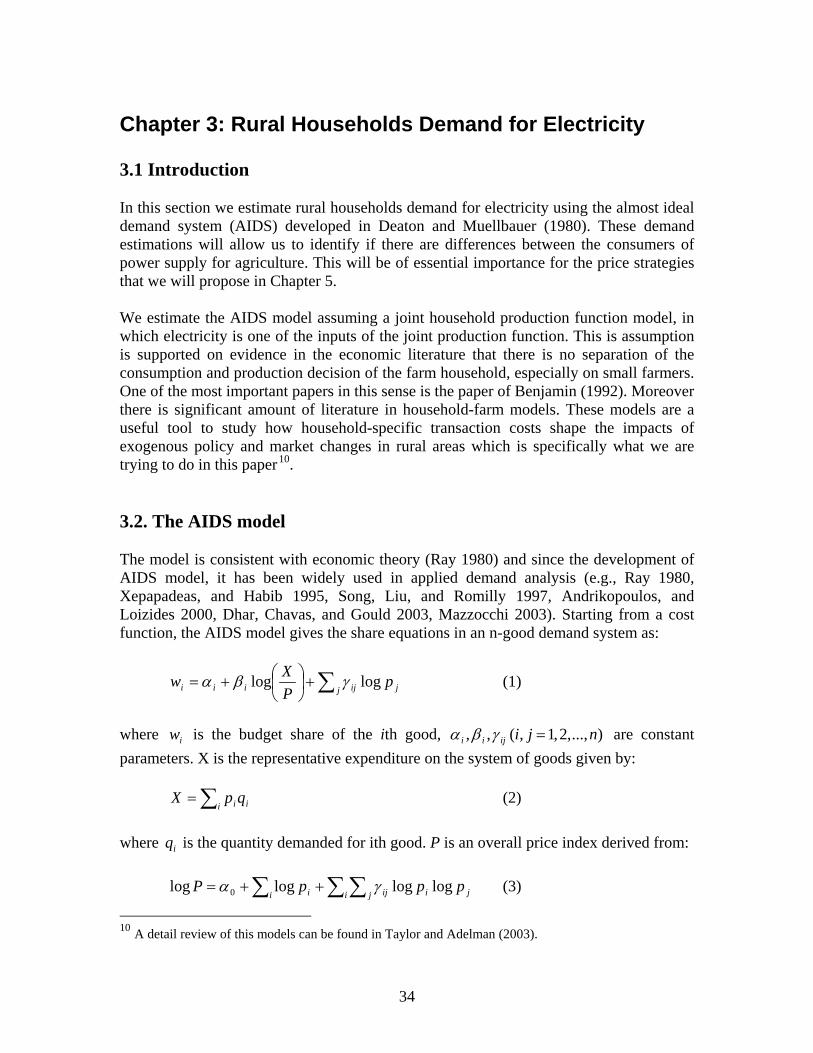
34
Chapter 3: Rural Households Demand for Electricity 3.1 Introduction In this section we estimate rural households demand for electricity using the almost ideal demand system (AIDS) developed in Deaton and Muellbauer (1980). These demand estimations will allow us to identify if there are differences between the consumers of power supply for agriculture. This will be of essential importance for the price strategies that we will propose in Chapter 5. We estimate the AIDS model assuming a joint household production function model, in which electricity is one of the inputs of the joint production function. This is assumption is supported on evidence in the economic literature that there is no separation of the consumption and production decision of the farm household, especially on small farmers. One of the most important papers in this sense is the paper of Benjamin (1992). Moreover there is significant amount of literature in household-farm models. These models are a useful tool to study how household-specific transaction costs shape the impacts of exogenous policy and market changes in rural areas which is specifically what we are trying to do in this paper�F
10. 3.2. The AIDS model The model is consistent with economic theory (Ray 1980) and since the development of AIDS model, it has been widely used in applied demand analysis (e.g., Ray 1980, Xepapadeas, and Habib 1995, Song, Liu, and Romilly 1997, Andrikopoulos, and Loizides 2000, Dhar, Chavas, and Gould 2003, Mazzocchi 2003). Starting from a cost function, the AIDS model gives the share equations in an n-good demand system as:
∑+⎟⎠⎞
⎜⎝⎛+=
j jijiii pPXw loglog γβα (1)
where iw is the budget share of the ith good, )...,,2,1,(,, njiijii =γβα are constant parameters. X is the representative expenditure on the system of goods given by:
∑=i iiqpX (2)
where iq is the quantity demanded for ith good. P is an overall price index derived from:
∑ ∑∑ ++=
i j jiiji i pppP loglogloglog 0 γα (3)
10 A detail review of this models can be found in Taylor and Adelman (2003).

35
Demand theory requires that the following conditions – adding-up, homogeneity, and symmetry – be satisfied:
0,0,1 === ∑∑∑ i iji ii i γβα (4)
01
=∑=
n
iijγ (5)
jiij γγ = (6) We will make two adjustments in this model: First, we will replace the price index given by (3) by Stone (1953) index: ∑=
k kk pwP loglog * (7) This will allow us a linear approximation of the nonlinear AIDS model. The resulting linear system, LA-AIDS (Linear Approximate Almost Ideal Demand System), is:
∑∑ +−+=
j jijk kkiii ppwXw log]log[log γβα (8)
Deaton and Muellbauer (1980) compared results between nonlinear approximation and the linear approximation using Stone Index on British data and found very little difference. Second, we will include a household size variable to adjust for the effects of economics of household size. Household demographic effects are found to be important determinants of household demand (Pollack and Wales 1980, 1981) and practiced in AIDS estimation (Ray 1980, Song, Liu, and Romilly 1997). Replacing X by mx where m and x denote family size and per capita expenditure on X, respectively, the estimable model is:
iij jijk kkiii vmppwxw +++−+= ∑∑ loglog]log[log θγβα (9)
A convenient property of this demand system is linearity, and each equation contains identical regressors. In the absence of across-equation restrictions, single-equation ordinary least squares estimation is therefore fully efficient (Nicol 1989). 3.3 Data Our data are drawn from National Sample Survey (NSS) 55th round. It is a periodic budget survey conducted in India’s all state and in rural and urban areas by the National Survey Organization of the Government of India. To our knowledge, the NSS is the only nationally representative survey to collect detailed information from individual households about expenditures on electricity, other fuel, and on food and non-food

36
expenditures. A detailed description of NSS 55th round data could be found in NSSO (2000) and other NSSO reports available in: http://mospi.nic.in/nsso.htm. We have broken households expenditures into nine groups: four subgroups for food expenditures: 1. Food grains; 2. pulses, edible oil, milk, egg, fish, and meat; 3. vegetables, fruits and sugar; 4. all other food; four subgroups for fuel and lighting: 5. electricity, 6. kerosene, 7. L.P.G, and 8. other fuel and light; and one group for all other nonfood expenditures: 9. all other non-food items. Our grouping of food expenditures into four groups is based on the assumption that intra-food allocation mechanism of a household is independent of its consumption decision on the fuel and light. By the same token, we have kept all non-food items into a single group. We have made four sub-groups within the category of expenditures on fuel and light. Since we are concerned with the electricity expenditure, dividing the fuel and lighting expenditures into multiple sub-groups is necessary to see the interdependence among different fuel categories. The four sub-groups within fuel and lighting are based on economic rationale as well as the nature of the data at hand. The obvious rationale of various sub-grouping within fuel is to allow for inter-fuel substitution. In NSS 55th round, expenditures on fuel and light included marketed items such as electricity, and kerosene, and non-marketed items such as gobar gas, and dung cake that make the aggregation complicated and estimation of implicit prices questionable. Besides non-marketability, some items such as firewood and chips are bought in infrequent intervals. That means expenditures outside the 30 days interval used that is for data collection may not be recorded. All these turn expenditures on fuel and light other than on electricity, kerosene, and LPG as exceptionally noisy. As a result, we include all of these under “expenditure on other fuel”. Table 3.2 shows the summary statistics of total household (HH) expenditures, shares of electricity in HH expenditure, and electricity prices. They are arranged in four expenditure quartiles presented in ascending order of expenditures. It is obvious from Table 3.2 that the distribution of households’ expenditure, the share of electricity, and prices – all are different between AP and PJ. There are state specific factors that need to be taken into account. These are the three primary variables that we are interested in calculating household’s demand for electricity in the short-run. In the long run, households’ demand for electricity is a joint demand determined by the stock of electrical equipments and its rate of use (Baker, Blundell, and Micklewright 1989). However, in the short run, changes in electricity prices should affect the rate of use only since stock of electrical equipments cannot be adjusted immediately. In the specific case of rural India, ownership of household durables that require electricity is not widely held (See Table A4a in Appendix for the yearly expenditures on electric equipments and its share on total household expenditures). These two factors – short-run nature of our data, and low-durable ownership – permit us to ignore the stock of electrical equipments in our estimation.

37
Table 3.2: Household Expenditures, Implicit Prices and Share of Electricity in Expenditure
Number of Household Expenditure Shares of Electricity in HH Exp.
Electricity Prices
Observations Mean Stdev Mean Stdev Mean Stdev AP Quartile 1 844 11869 3244 0.037 0.017 0.992 0.405 Quartile 2 874 18790 1546 0.030 0.013 0.999 0.334 Quartile 3 893 25466 2369 0.028 0.014 1.038 0.345 Quartile 4 852 44023 16618 0.025 0.017 1.115 0.497 All 3530 24823 14567 0.030 0.016 1.046 0.524 PJ Quartile 1 493 20976 5179 0.061 0.034 1.991 1.162 Quartile 2 464 33177 3134 0.055 0.032 2.107 1.700 Quartile 3 487 46534 4979 0.050 0.032 1.942 0.988 Quartile 4 496 86697 60826 0.042 0.031 2.014 1.271 All 2020 46605 39104 0.052 0.033 2.004 1.233 Source: NSS 55th round; Stdev: Standard Deviation. 3.4 Results Table 3.3 presents the parameter estimates for unrestricted model. The parameters are elect_real: real expenditure; elect_p_ln: own price of electricity; kerosene_pw: kerosene price; fuel_oth_pw: other fuel price, lpg_pw: LPG price; f1_pw: food grains price; f2_pw: pulses, edible oil, milk, egg, fish, and meat price; f3_pw: fruits, vegetables and sugar price;f4_pw: All other food;n_f5_pw: non-food, ln_hh_size: household size; and constant. These parameters are estimated for all households confined to rural areas of AP and Punjab only, and there are estimates for AP and Punjab (labeled as All) together and for each of the states separately. Based on equation (9), different elasticities – expenditure ( iex ), own-price ( iiep ), cross-price ( ijep ), and size ( ine ) – are given by:
iii wex /1 β+= (10)
iiiiii wep βγ −+−= /1 (11)
ijiiijij wwwep // βγ −= (12)
iii wne /θ= (13) Table 3.3 presents own price (uncompensated) elasticities. All elasticities are calculated at mean budget share using unrestricted parameters presented in Table 3.3 and equations (10) to (13). The own price elasticity for both Punjab and AP is -0.5192, while it is -0.666 for AP and -0.8458 for Punjab, i.e. rural households are more elastic in the case of Punjab then in AP.

38
Table 3.3
Almost Ideal Demand System (AIDS), by region All AP Punjab
elect_real 0.0119 0.0099 0.0186(0.0004)*** (0.0004)*** (0.0009)***
elec_p_ln 0.0184 0.0103 0.0088(0.0007)*** (0.0008)*** (0.0018)***
kerosene_pw -0.0330 -0.0299 -0.0243(0.0077)*** (0.0067)*** (0.0137)*
fuel_oth_pw -0.0808 -0.0546 -0.0845(0.0024)*** (0.0024)*** (0.0043)***
lpg_pw -0.0307 -0.0400 -0.0485(0.0065)*** (0.0061)*** (0.0136)***
f1_pw 0.0007 -0.0089 -0.0322(0.0014) (0.0012)*** (0.0047)***
f2_pw -0.0018 0.0002 0.0049(0.0014) (0.0015) (0.0022)**
f3_pw 0.0026 0.0067 0.0092(0.0028) (0.0026)*** (0.0055)*
f4_pw 0.0062 0.0032 0.0064(0.0010)*** (0.0008)*** (0.0033)*
n_f5_pw -0.0019 -0.0106 0.0007(0.0027) (0.0031)*** (0.0041)
ln_hh_size 0.0005 -0.0045 0.0020(0.0005) (0.0005)*** (0.0011)*
Constant -0.0786 -0.0575 -0.1310(0.0044)*** (0.0042)*** (0.0081)***
Observations 5319 3439 1880R-squared 0.603 0.558 0.591
Elasticity (own price) -0.5192 -0.6666 -0.8458
Source: 55th Round of the National Sample Survey.
Notes: 1. A different price for each household was calculated using the information for
expenditure in electricity and Kw consumed. As no price could be calculated for households without any consumption of electricity, they were excluded from the sample.
2. Usual procedures for detection of outliers, inconsistencies and atypical values, according to the distribution of variables in the regression, were applied.
11/8/2007 39
Interestingly, size – the economics of households has opposite effects for AP compared to Punjab. While there is an economics of scale for AP implying that household’s per capita expenditure share of electricity decreases as household size increases, there is a diseconomy of scale for the Punjab implying that household’s per capita expenditure share of electricity increases with household size. One explanation is the stock of durables and utilization rate that might have a non-linear relationship after crossing an income (expenditure) threshold. However, this issue asks for explanations that are beyond the scope of the current study. Kerosene is a potential substitute of electricity for some usages, for lighting, for instance. The results shows that this is the case, both in AP and Punjab the cross price elasticity of kerosene is negative making kerosene a substitute of electricity. Although, kerosene is supplied from two sources in India: public distribution system – which is subsidized and charges fixed price, and market system, and our data did not allow us to differentiate these two sources. Although to be able to differentiate producers according to their intensity of use of electricity to pump water for irrigation we needed to identify the demand of electricity according to the extension of irrigated land. Table 3.4. present the results obtained when we classify the irrigated land extension in three groups: marginal or small from more than 0 hectares to 1.8 hectares; medium from more than 1.8 hectares to 3.64 hectares; and large from more than 3.64 hectares. As expected the results show that the bigger the size of the irrigated land the more inelastic the demand is. This result is very clear for Andrah Pradesh where the own price elasticity is -0.6877 for marginal or small farmers and -0.4955 for large land extensions. In the case of Punjab the eleasticities move from -0.9074 to -0.8586 for marginal/small and large extension of irrigated land respectively. The existence therefore of different demands according to the extension of irrigated lands will allow us to implement a strategy of price discrimination to better assign subsidies as will be explained in the following chapter.

11/8/2007 40
Table 3.4 Almost Ideal Demand System (AIDS), by region and extension of irrigated lands
Marginal / Small Medium Large Marginal / Small Medium Large] 0 ha - 1.8 ha ] ] 1.8 ha - 3.64 ha ] ] 3.64 ha + [ ] 0 ha - 1.8 ha ] ] 1.8 ha - 3.64 ha ] ] 3.64 ha + [
elect_real 0.0119 0.0128 0.0130 0.0183 0.0170 0.0152(0.0008)*** (0.0015)*** (0.0020)*** (0.0018)*** (0.0025)*** (0.0025)***
elec_p_ln 0.0091 0.0124 0.0148 0.0057 0.0051 0.0066(0.0014)*** (0.0030)*** (0.0025)*** (0.0038) (0.0050) (0.0038)*
kerosene_pw -0.0178 -0.0211 0.0776 -0.0358 -0.1309 -0.1248(0.0158) (0.0222) (0.1020) (0.0395) (0.0796) (0.0624)**
fuel_oth_pw -0.0557 -0.0616 -0.0902 -0.0908 -0.1056 -0.0923(0.0048)*** (0.0115)*** (0.0176)*** (0.0082)*** (0.0135)*** (0.0179)***
lpg_pw -0.0227 -0.0480 0.0002 -0.0395 -0.0754 -0.0621(0.0109)** (0.0160)*** (0.0291) (0.0306) (0.0399)* (0.0347)*
f1_pw -0.0119 -0.0220 -0.0183 -0.0267 -0.0320 -0.0233(0.0020)*** (0.0045)*** (0.0062)*** (0.0088)*** (0.0171)* (0.0136)*
f2_pw 0.0005 -0.0138 -0.0198 0.0042 0.0037 0.0068(0.0025) (0.0058)** (0.0088)** (0.0042) (0.0061) (0.0045)
f3_pw -0.0001 -0.0006 0.0161 -0.0010 -0.0046 -0.0147(0.0041) (0.0080) (0.0118) (0.0099) (0.0151) (0.0140)
f4_pw 0.0056 0.0112 0.0141 0.0136 0.0238 0.0097(0.0015)*** (0.0031)*** (0.0046)*** (0.0048)*** (0.0113)** (0.0085)
n_f5_pw -0.0143 0.0017 0.0084 -0.0031 0.0034 0.0199(0.0051)*** (0.0068) (0.0188) (0.0116) (0.0124) (0.0084)**
ln_hh_size -0.0010 -0.0007 -0.0025 0.0075 -0.0023 0.0006(0.0009) (0.0017) (0.0021) (0.0023)*** (0.0031) (0.0028)
Constant -0.0806 -0.0990 -0.0951 -0.1344 -0.1173 -0.1108(0.0074)*** (0.0129)*** (0.0181)*** (0.0153)*** (0.0229)*** (0.0226)***
Observations 938 169 92 553 187 211R-squared 0.546 0.720 0.755 0.574 0.724 0.636
Elasticity -0.6877 -0.5527 -0.4955 -0.9074 -0.9119 -0.8586
Andhra Pradesh Punjab
Source: 55th Round of the National Sample Survey. Notes: 1. A different price for each household was calculated using the information for expenditure in electricity and Kw consumed. As no price could be
calculated for households without any consumption of electricity, they were excluded from the sample. 2. In the classification of households, those with no irrigated lands were also excluded. 3. Usual procedures for detection of outliers, inconsistencies and atypical values, according to the distribution of variables in the regression, were
applied.

11/8/2007 41
Chapter 4: Price Discrimination as a Solution 4.1 Introduction As shown in the previous chapters, particularly in Chapter 2, it is clear that there is a need to identify alternative institutional mechanisms to reduce inefficiency in assigning the subsidy, and to gradually reduce the subsidy to improve quality and quantity of power and to reduce the growing trend of environmental damage. To be able to tackle this problem it is essential to establish a pricing mechanism that could improve the current situation. In this chapter we propose a strategy of price discrimination based on the size of the farmers plot and on the implementation of a series of possible two part tariff mechanisms. We will present a set of simulations for three price schemes which try to progressively move from a better targeted subsidy to a final scheme where the subsidy is minimized or eliminated. In the first price scheme the first part of the tariff will be equivalent to the value of the average current consumption of the small holders, which will, at the same time, be the amount of the subsidy. This will assure that on the one hand, the small holders will on average not be affected by this new price mechanism, and on the other hand, the subsidy will be better targeted. The second part of the tariff will be set at the level of the marginal cost in such a way that high demanders will cover their costs for any consumption above the minimum allowed by the first part of the tariff. In the second price mechanism we apply the same two part tariff mechanism but we allow for two variable tariffs. As in the previous case the first part of the tariff will be equivalent to the value of the average current consumption of the small holders so that they keep the current subsidy and their consumption is not changed. The two variable tariffs will be targeted to higher levels of consumption and will be optimized in such a way the total subsidy is minimized. As a result the high demanders for electricity will end paying average prices higher than their marginal costs and will be therefore cross subsidizing the small holders. As a result the burden of the subsidy will be reduced. Finally, the third price mechanism moves towards the elimination of the subsidy and allows the three tariffs to vary. Although, we belief this third alternative can not be implemented immediately we believe that through appropriate cross subsidy mechanisms it can be implemented in the future. Although it will be ideal to install electric meters first to implement these three price schemes it was clear from several meetings with policy makers and farmers that starting with the meters was not politically viable. This is an extremely political issue and that’s the reason why we a proposing a progressive mechanism towards electric meters. Our belief is the price discrimination mechanism based on land size will give the correct incentives to farmers to accept meters. Specifically, if a farmer beliefs that the prices

11/8/2007 42
through the proposed mechanism does not approach to his reality then he will have all the incentives to ask for a meter to be charged exactly what he consumes. Finally, and just as an additional sensitivity analysis to the elasticities used we estimate in Appendix B the three price discrimination scenarios using Kumar and Shukla (1999) estimation of elasticies for electric demand in India of -1.35. This elasticity is estimated based on time series data for 9 years (from 1985/86 to 1993/94) pooled over 19 Indian States (which includes Punjab and Andhra Pradesh). 4.2 Price discrimination and two part tariffs Price discrimination occurs when a producer sets different prices for the same product. Specifically in our case we will be talking of kilowatt hours of electricity supplied to the farmers. In order for a firm to be able to successfully engage in price discrimination, the following conditions must hold: the firm must have some degree of market power in such a way that it can establish different prices; the firm must be able to identify consumers based on which they can discriminate; and no resale can occur (no arbitrage) because through re-sale the effects of price discrimination will end being perverse. All of these assumptions clearly hold for the two states under study. There are three ways to price discriminate: first-degree price discrimination, second degree price discrimination and third degree price discrimination. First degree price discrimination which is also known as perfect price discrimination occurs when a monopolist charges a different price for each unit sold to each consumer. With perfect price discrimination a consumer pays exactly what she is willing to pay for each unit, thus consumer surplus (i.e. the difference between what a consumer is willing to pay and what they actually pay) is zero. Even though consumer surplus is zero in a market with a monopolist engaging in first-degree price discrimination, total surplus is maximized; that is, there is no deadweight loss. This occurs because the monopolist will sell until the revenue from the last unit sold is equal to the cost of that last unit. Previously, when a monopolist charged only one price (uniform, or linear, pricing), marginal revenue was less than the price a consumer was willing to pay for the last unit purchased. Here, however, marginal revenue is equal to the willingness to pay of the consumer. If the monopolist sells one more unit, she will earn whatever the consumer is willing to pay (represented by the inverse demand curve) for that unit. This implies that selling until marginal revenue is equal to marginal cost will lead to an equilibrium output where the quantity the market demands is equal to marginal cost. Imperfect price discrimination occurs when a monopolist sets different prices for different groups of people. We break imperfect price discrimination into two categories: second- and third degree price discrimination. Second-degree price discrimination occurs when multiple prices are offered for different units of the same product. A menu of offered prices allows consumers to segment themselves into various types when the monopolist is unable to successfully identify different groups through other means (such as asking for identification). This type of

11/8/2007 43
discrimination is what we normally see in cellular phone pricing in which households according to their needs of calling time will self select themselves in different price plans. Third-degree price discrimination occurs when a firm can identify different types of consumers and charge them different prices based on who they are. For example, in our specific case we can identify consumers by the size of their land and therefore charge them different prices according to land size. We assume that consumers with small possessions of land have a lower ability to pay for electricity because of their low incomes. We can say that perfect price discrimination leads to an increase in total surplus, although society suffers a decrease in consumer surplus. However, when moving from a single market price to a situation in which a firm engages in third-degree price discrimination we cannot say whether consumers are better or worse off. The outcome will depend on the cost and demand conditions for that particular market. Consider the following example. Suppose that the power company services two types of customers: big farmers and small farmers. The company can easily tell which is which. Lets 1 denote large farmer and 2 denote small farmer and lets assume that each type of farmer have the following demands: Q1 = 20 – P and Q2 = 5 – P. For simplicity, assume the marginal cost and fixed cost for the power company are zero. The results of price and not price discrimination are summarized in the following table.
Table 4.1 Comparing Price versus non Price Discrimination
Results without price discrimination, i.e.
same price for both consumers Results with price discrimination, i.e.
different price for both consumers Equilibrium condition is Marginal revenue (MR)=Marginal Cost (MC) and demands are added horizontally
Firm can act as a monopolist in each market, so MR1=MC1 and MR2=MC2
Demand Dtot= Q1 + Q2 = 20 – P + 5 – P = 25 – 2P for P < 5 = Q1 = 20 – P for P > 5 Solving for prices: P = 12.5 – Q for P < 5 = 20 – Q for P > 5
Demand: D1=20-P D2=5-P
Equilibrium: 20-2Q = 0, therefore Q*=10, P*=10
Equilibrium MR1=20-2Q1=0, therefore: Q1 = 10 and P1 = $10 MR2 =5 –2Q2 =0 therefore: Q2 = 2.5 and P2 = $2.50
Profits of the Operator Π = (P – MC)*Q = 10*10 = 100
Profits of the Operator Π = (P1 – MC)*Q1 + (P2 – MC)*Q2 = 10*100 + 2.5*2.5 = 106.25
Total Welfare (TW): Total Welfare(TW) = CS1 + CS2 + Π = ½(20 – 10)*10 + 0+100 = 150
Total Welfare (TW): Total Welfare(TW) = CS1 + CS2 + Π = ½(20 – 10)*10 + ½(5-2.5)*2.5 + 106.25 = 159.375

11/8/2007 44
Two-part Tariffs If the monopolist is unable to engage in first-degree price discrimination an alternative is to use two part tariff. In two part tariffs the first part is a fixed fee for right to use the good or service and normally implies a fixed number of units of the good; and in the second part a price is charged per unit for the good consumed. The question is how will the operator decide what the fixed fee and per-unit price will be? If there are multiple types of consumers, but the monopolist can post only a single two-part tariff, then there may be reason to exclude some types from the market altogether. Consider the case of two consumer types—big demanders (i.e, large owners of land) and small demanders (small holders)—and assume that the firm will set unit price at marginal cost. Then the firm has two main options: (i) it can either serve both, setting the two-part tariff to extract the low demander’s full surplus, leaving the high demander with positive surplus, or (ii) serve only the high demander and extracting his full surplus. In either case the unit price will be set at marginal cost while the fixed fee extracts all of one of the two type’s consumer surplus at that price. Whether it is profitable to go from option (i) to option (ii) depends on whether the loss of revenue from low demanders is more than made up by increased charges (in the form of higher fixed fees) on high demanders. Under option (i), the firm earns profit of 2*CS1, whereas under option (ii) it earns CS2. Therefore, excluding the low demanders is profitable, provided 2*CS1 < CS2 or CS2 - CS1 > CS1. The figure below depicts this condition as a comparison of the relative sizes of two shaded areas. P CS2 – CS1 MC = $1 D(p) Q of electricity consumption In the following sections of this chapter we will try to implement this two part tariff mechanism to the rural electricity consumers of Andhra Pradesh and Punjab. The strategy will essentially consist of dividing farmers by the land possession and then keeping the level of subsidy on the first part of the tariff in such a way that smallholders are not affected by the second part of the tariff. As a result, we will assure that the distribution of the subsidy is significantly more progressive and better distributed than what is currently being done. 4.3 Simulating impacts of a two part tariff – Simulation 1
11/8/2007 45
The simulation of demand under the implementation of a two-part tariff involved primarily two different data sets. The first one was the 54th Round of the National Sample Survey (NSS). This dataset provided us with accurate information on the lands owned by households in the Andhra Pradesh and Punjab regions of India. The second was the 55th Round of the NSS, which included information on households’ consumption of electricity in these regions under our assumption of a joint household production function. The latter was useful to estimate demand elasticities and measure the impact of changes in pricing policy as shown in Chapter 4. Using information from the 54th Round of the NSS, households were classified in three categories (small, medium, and large landholders), according to their lands with electric-pump irrigation. In Andhra Pradesh households with less than 1.9 ha irrigated with electric pumps were classified as small. Those with more than 1.8 ha but less than 3.64 ha were included in the second range; and those with more than 3.64 ha, in the third one. An analogous classification was also done for Punjab households: those with less than 1.9 ha were considered as smallholders; those with more than 1.9 ha but less than 3.98 were regarded as medium; and those with more than 3.98 ha, as large. Among these three groups, two different types of crops were identified according to their intensity of use of water: (a) wheat and other cereals, pulses, oils seeds, mixed crops, sugar cane, vegetables, fodder, fruits and nuts, and others; and (b) paddy. On the other hand, information of the 55th round allowed us to estimate Almost Ideal Demand Systems –AIDS as shown in the previous chapter. Nevertheless, there were some difficulties applying the same categories used in the 54th round to the 55th Round of NSS. Even when the latter included data on whether the land was irrigated or not, it did not provide with information on the kind of irrigation used by the households. Thus, elasticities were estimated according to household’s irrigated lands instead of irrigated lands with electric-pump irrigation. Differences in the information collected by survey could not prevent this shortcoming. But as previously mentioned all the simulations are based on information from NSS 5th round that did allow us to identify lands that were irrigated with electric pump irrigation. Therefore we are not over estimating the irrigated land given that we only use the 54th round for the simulations, but we could have a small bias on the calculation of the elasticities. Household’s expenditure in electricity within each category was estimated through a set of assumptions. Firstly, a certain kind of motor was assumed for each category: 0-3 HP (average of 1.5 HP) motors for smallholders, 3-5 HP (average of 4 HP) for medium landholders, and 5 - 7.5 HP (average of 6.3 HP) for large landholders. Next, conversion factors were used to estimate households’ demand for electricity in each category. Two pairs of conversion factors were given for cultivation of paddy and wheat and others. According to this information, a 5 HP motor may require 414 kw/ha to irrigate one ha of wheat and 1426 kw/ha to irrigate one ha of paddy; while a 10 HP motor may require 290 kw/ha for wheat and 998 for paddy. Assuming this distribution, we extrapolated points for the average motor among smallholders, medium, and large landholders. Finally, a fixed charge was assigned, according to the average motor in each category, based on the prices presented in the India’s Tariff Order 2003-2004.

11/8/2007 46
The two part payment schedule proposed here establishes an initial quantity q1, priced at p1; while demand exceeding q1 units is priced at marginal cost p2. To estimate households’ demand for electricity under the new scheme, we needed to assign changes in prices for each category of landholders. Thus, two part tariff schedule with two conditions were conceived. Firstly, expenditure of smallholders should not be affected by changes in pricing scheme, so that the smallholders won’t be affected by the proposed tariff mechanism. In this sense, q1 and p1 were established as the average quantity and price in the electricity demand of smallholders (without affecting electricity expenditure among smallholders). Consumption exceeding q1 in the other two categories (q2) is priced at the marginal cost p2. Marginal cost is assumed to be equal to the highest average price among the three categories of landholders in the 55th Round of NSS. Considering estimated expenditure in each category (p1q1 + p2q2) and total consumption (q1+ q2), weighted average price is calculated. The latter allows calculation of percentage change of price between the actual situation and the simulation. With this change and elasticities formerly estimated, we were able to find new consumption levels of the three categories of landholders as shown in Tables 4.2a and 4.2b. In both regions, Punjab and Andhra Pradesh, as expected the results show that for the small or marginal producers their consumption is not affected while the consumption for the medium and large producers is reduced. Specifically, in the case of Andhra Pradesh the consumption of electricity under the proposed two part tariff scheme will be reduced by 14% and 41%, respectively. The small producers under this two part tariff scheme will face the same weighted average price, i.e. 0.40 ruppies per kwh, while the medium and large producers will face an increase of 25.1% and 82.2% in their weighted average prices. The latter implies that the price for the medium producers will increase from 0.70 to 0.87 ruppies per kwh, while the price for the large producers will increase from 0.58 to 1.05 ruppies per kwh. This increase reflects the fact that the large producers consume more than six times the amount of kwh that the small or marginal producers consume and therefore under the current fixed tariff scheme they where the ones mostly benefiting from the electricity subsidies as described in Chapter 2. Similarly, and as shown in Table 4.2b, in the case of Punjab the consumption of electricity of small or marginal producers will remain constant, while the consumption for medium and large producers will be reduced in -0.16% and -0.47% respectively. The small producers under this two part tariff scheme will face the same weighted average price, i.e. 1.06 rupies per kwh, while the medium and large producers will face an increase of 17.1% and 55.3% in their weighted average prices. The latter implies that the price for the medium producers will increase from 0.97 to 1.14 ruppies per kwh, while the price for the large producers will increase from 0.75 to 1.16. This increase reflects the fact that the large producers consume more than six times the amount of kwh that the small or marginal producers consume and therefore under the current fixed tariff scheme they where the ones mostly benefiting from the electricity subsidies as described in Chapter 2.

11/8/2007 47
Table 4.2a Summary of Simulation 1: Andhra Pradesh
Land size (Ha) Crop % of sample Average Ha (total) Average Ha Motor (HP) Average HP kwh / Ha Charge Rs/HP/Year Actual exp
] 0 - 1.8 ] Wheat 0.36 ] 0 - 3 ] 1.5 500.8] 0 - 1.8 ] Paddy 0.38 ] 0 - 3 ] 1.5 1725.6
] 1.8 - 3.64 ] Wheat 1.45 ] 3 - 5 ] 4.0 438.8] 1.8 - 3.64 ] Paddy 1.00 ] 3 - 5 ] 4.0 1511.6
] 3.64 + [ Wheat 3.30 ] 5 - 7.5 ] 6.3 383] 3.64 + [ Paddy 2.94 ] 5 - 7.5 ] 6.3 1319
Land size (Ha) Crop kw price Exp kw price Exp] 0 - 1.8 ] Wheat] 0 - 1.8 ] Paddy
] 1.8 - 3.64 ] Wheat] 1.8 - 3.64 ] Paddy
] 3.64 + [ Wheat] 3.64 + [ Paddy
Land size (Ha) Crop] 0 - 1.8 ] Wheat] 0 - 1.8 ] Paddy
] 1.8 - 3.64 ] Wheat] 1.8 - 3.64 ] Paddy
] 3.64 + [ Wheat] 3.64 + [ Paddy
total kw
Simulated q % change in q
Simulation
840.47 0.40 337.50
Information on land size
225
375
0.75
2.45
71.33
Potential expenditure
338
1500
2969
Actual exp
16.63
12.05
Two-part tariff
4756.24
1.18 1538.88
840.47 0.40 337.50
840.47 0.40 337.50
4298.13 1.18 5071.80
840.47
2144.60
5138.60
0.00 1.18 0.00
1304.13
First part Second part Total expenditure
Weighted Avg price Price t=0
0.40
0.70
0.58
% change price
0.0%
25.1%
82.2%
-0.69
-0.55
-0.50
337.50
1876.38
5409.30
0.40
0.87
1.05
Elasticity
840.47
1847.20
3045.45
0.00
-0.14
-0.41

11/8/2007 48
Table 4.2b Summary of Simulation 1: Punjab
Land size (Ha) Crop % of sample Average Ha (total) Average Ha Motor (HP) Average HP kwh / Ha Charge Rs/HP/Year Actual exp] 0 - 1.9 ] Wheat 0.69 ] 0 - 3 ] 1.5 500.8] 0 - 1.9 ] Paddy 0.24 ] 0 - 3 ] 1.5 1725.6
] 1.9 - 3.98 ] Wheat 1.81 ] 3 - 5 ] 4.0 438.8] 1.9 - 3.98 ] Paddy 0.95 ] 3 - 5 ] 4.0 1511.6
] 3.98 + [ Wheat 5.16 ] 5 - 7.5 ] 6.3 383] 3.98 + [ Paddy 3.05 ] 5 - 7.5 ] 6.3 1319
Land size (Ha) Crop kw price Exp kw price Exp] 0 - 1.9 ] Wheat] 0 - 1.9 ] Paddy
] 1.9 - 3.98 ] Wheat] 1.9 - 3.98 ] Paddy
] 3.98 + [ Wheat] 3.98 + [ Paddy
Land size (Ha) Crop] 0 - 1.9 ] Wheat] 0 - 1.9 ] Paddy
] 1.9 - 3.98 ] Wheat] 1.9 - 3.98 ] Paddy
] 3.98 + [ Wheat] 3.98 + [ Paddy
First part Total expenditure
Potential expenditure Actual exp total kw
Elasticity Simulated q % change in q
Second part
42.73
0.94
2.76
8.21
30.73
26.55 540
720
810540
2160
4500
-0.91
-0.86
810.00 1.18
1456.77
5234.89
1.18
-0.91
810.00
1.06
Two-part tariff
1.06
Information on land size
0.00767.38
767.38
767.38
810.00
810.00
1.06
1.06
767.38
2224.16
6002.27
1.18
0.00
1718.99
6177.17
2528.99
1.14
6987.17
1.16
0.97 17.1%
0.75 55.3%
0.00
Simulation
Price t=0 % change price
1.06 0.0%
Weighted Avg price
-0.16
-0.47
767.38
1877.69
3154.04 :
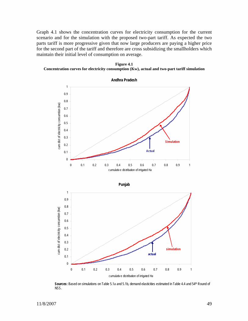
11/8/2007 49
Graph 4.1 shows the concentration curves for electricity consumption for the current scenario and for the simulation with the proposed two-part tariff. As expected the two parts tariff is more progressive given that now large producers are paying a higher price for the second part of the tariff and therefore are cross subsidizing the smallholders which maintain their initial level of consumption on average.
Figure 4.1 Concentration curves for electricity consumption (Kw), actual and two-part tariff simulation
Andhra Pradesh
0
0.1
0.2
0.3
0.4
0.5
0.6
0.7
0.8
0.9
1
0 0.1 0.2 0.3 0.4 0.5 0.6 0.7 0.8 0.9 1cumulativ e distribution of irrigated Ha
cum
dist
of e
lectri
city
cons
umtio
n (k
w)
Actual
Simulation
Punjab
0
0.1
0.2
0.3
0.4
0.5
0.6
0.7
0.8
0.9
1
0 0.1 0.2 0.3 0.4 0.5 0.6 0.7 0.8 0.9 1
cumulativ e distribution of irrigated Ha
cum
dist
of e
lectri
city
cons
umtio
n (k
w)
actualsimulation
Sources: Based on simulations on Table 5.1a and 5.1b, demand elasticities estimated in Table 4.4 and 54th Round of NSS.
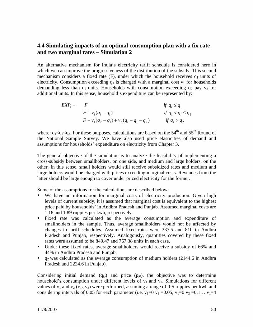
11/8/2007 50
4.4 Simulating impacts of an optimal consumption plan with a fix rate and two marginal rates – Simulation 2 An alternative mechanism for India’s electricity tariff schedule is considered here in which we can improve the progressiveness of the distribution of the subsidy. This second mechanism considers a fixed rate (F), under which the household receives q1 units of electricity. Consumption exceeding q1 is charged with a marginal cost v1 for households demanding less than q2 units. Households with consumption exceeding q2 pay v2 for additional units. In this sense, household’s expenditure can be represented by:
2212121
2111
1
)()()(
qqifqqqvqqvFqqqifqqvF
qqifFEXP
ii
ii
ii
>−−+−+≤<−+
≤=
where: q1<q2<q3. For these purposes, calculations are based on the 54th and 55th Round of the National Sample Survey. We have also used price elasticities of demand and assumptions for households’ expenditure on electricity from Chapter 3. The general objective of the simulation is to analyze the feasibility of implementing a cross-subsidy between smallholders, on one side, and medium and large holders, on the other. In this sense, small holders would still receive subsidized rates and medium and large holders would be charged with prices exceeding marginal costs. Revenues from the latter should be large enough to cover under priced electricity for the former. Some of the assumptions for the calculations are described below: We have no information for marginal costs of electricity production. Given high
levels of current subsidy, it is assumed that marginal cost is equivalent to the highest price paid by households’ in Andhra Pradesh and Punjab. Assumed marginal costs are 1.18 and 1.89 ruppies per kwh, respectively.
Fixed rate was calculated as the average consumption and expenditure of smallholders in the sample. Thus, average smallholders would not be affected by changes in tariff schedules. Assumed fixed rates were 337.5 and 810 in Andhra Pradesh and Punjab, respectively. Analogously, quantities covered by these fixed rates were assumed to be 840.47 and 767.38 units in each case.
Under these fixed rates, average smallholders would receive a subsidy of 66% and 44% in Andhra Pradesh and Punjab.
q2 was calculated as the average consumption of medium holders (2144.6 in Andhra Pradesh and 2224.6 in Punjab).
Considering initial demand (qio) and price (pi0), the objective was to determine household’s consumption under different levels of v1 and v2. Simulations for different values of v1 and v2 (v1< v2) were performed, assuming a range of 0-5 ruppies per kwh and considering intervals of 0.05 for each parameter (i.e. v1=0 v2 =0.05, v1=0 v2 =0.1… v1=4

11/8/2007 51
v2 =4.05, v1=4 v2 =4.1, v1=4 v2 =4.15… v1=4.95 v2 =5 ruppies per kwh). For each simulation, given qio, we estimated the change in household’s expenditure (Ei1), as it would be in the first, second or third section of the tariff schedule. With this new simulated expenditure level, we calculated the implicit price that the household is paying for each unit of electricity (pi1). With the variation in price and elasticities from the AIDS model, we were able to find a new demand (qi1). Nevertheless, as households do not adjust immediately to changes in the tariff schedule, a dynamic process was considered. Household’s simulated consumption qi1 was used to estimate new expenditure (Ei2), implicit price (pi2), and demand (qi2). As the optimal number of iterations was not clear, this process was performed seven times, obtaining values Ei7, pi7, and qi7, when relatively acceptable convergence was achieved. With these simulations, total revenue and costs of the electricity firm could be found.
Assuming linear cost function, total cost will be ∑=
n
iiqMgC
17 , while total revenue will be
equivalent to ∑=
n
iiE
17 . With total cost and revenue, a profit function is calculated (Figure
4.2). According to the results of this simulation, the impact on total electricity subsidy and its distribution are reported for different values of v1 and v2. As clearly shown in Figure 4.2 there is a positive relation between v1, v2 and the profits of the firm. Our objective was therefore to simulate different scenarios with different levels of v1 and v2 such to identify the possible impact in the resulting subsidy relative to the current level of subsidy in AP and Punjab. The results are presented in Table 4.3a and 4.2b for Andhra Pradesh and Punjab, respectively. In the case of Andhra Pradesh with tariffs of v1=2 and v2=3.45 the subsidy is reduced to 33% of the current subsidy and large holders are cross subsidizing small holders, as shown in the negative ratio of subsidy of small holders divided by the subsidy of the large holders. For the case of Punjab the prices of v1 and v2 will have to be 4.9 and 5 to be able to arrive to a similar scenario. These results are because the land ownership is far more concentrated in Punjab than in Andhra Pradesh and therefore under the current situation the subsidies are clearly benefiting a lot more the large holders. Figure 4.3a and 4.3b present the same results for both states. These graphs show the distribution of the subsidies under different combinations of v1 and v1 and for different types of farmers (small holders, medium holders, and large holders). Similarly, the results show that for Punjab higher tariffs are needed for medium and large holders to be able to arrive to a situation in which part of the subsidy to the small holders is being covered by large holders.
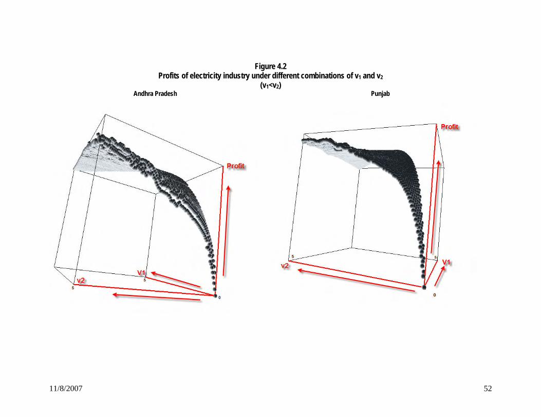
11/8/2007 52
Figure 4.2 Profits of electricity industry under different combinations of v1 and v2
(v1<v2) Andhra Pradesh
Punjab

11/8/2007 53
According to the graphs, in Punjab v1 needs to be 4.9 ruppies per kwh and v2 needs to be 5 ruppies per kwh to arrive a situation where small holders receive the same subsidy as they currently do, medium holders still receive subsidy although smaller than what they do under the current distribution, and the large holders pay part of the subsidies given to the small and the medium.
Table 4.3a Summary of Simulation 2, selected values of v1 and v2
Andhra Pradesh
1 2 3 4 5 6
Assumptions
Marginal Cost 1.18 1.18 1.18 1.18 1.18 1.18 Fixed rate (F) 337.5 337.5 337.5 337.5 337.5 337.5 Units included in fixed rate (q1) 840.47 840.47 840.47 840.47 840.47 840.47 Subsidy fixed rate (% MgC) 66.0% 66.0% 66.0% 66.0% 66.0% 66.0%
Parameters
v1 0.00 0.40 0.60 1.10 2.00 2.70 v2 0.00 0.75 1.55 2.20 3.45 5.00
Impact
Simul Subs / Actual Subs 2.19 1.00 0.75 0.50 0.33 0.27 Subs smallholders / largeholders
Actual 1.04 1.04 1.04 1.04 1.04 1.04 Simul 0.60 1.32 2.56 4.65 -23.49 -10.43
In the case of Andrah Pradesh v1 need to be 2 ruppies per kwh and v2 needs to be 3.45 ruppies per kwh to arrive to a similar situation as Punjab. On the other hand when v1 is 2.70 ruppies per kwh and v2 is 5 ruppies per kwh also medium holders start to cross subsidize small holders. Therefore this pricing strategy is substantially more progressive than the current situation.

11/8/2007 54
Table 4.3b Summary of Simulation 2, selected values of v1 and v2
Punjab
1 2 3 4 5 6
Assumptions
Marginal Cost 1.89 1.89 1.89 1.89 1.89 1.89 Fixed rate (F) 810 810 810 810 810 810 Units included in fixed rate (q1) 767.38 767.38 767.38 767.38 767.38 767.38 Subsidy fixed rate (% MgC) 44.2% 44.2% 44.2% 44.2% 44.2% 44.2%
Parameters
v1 0.00 0.15 0.35 0.60 0.90 4.90 v2 0.00 0.80 1.05 1.60 2.10 5.00
Impact
Simul Subs / Actual Subs 2.64 1.00 0.75 0.50 0.33 0.02 Subs smallholders / largeholders
Actual 0.05 0.05 0.05 0.05 0.05 0.05 Simul 0.04 0.07 0.10 0.17 0.28 -16.79

11/8/2007 55
Figure 4.3a Distribution of electricity subsidy, selected values of v1 and v2
(% of total subsidy)
A. Andhra Pradesh
v1=0, v2=0
0%
10%
20%
30%
40%
50%
60%
Smallho lders M edium ho lders Large ho lders
ActualSimulation
v1=0.40, v2=0.75
0%
5%
10%
15%
20%
25%
30%
35%
40%
45%
50%
Smallho lders M edium ho lders Large ho lders
ActualSimulation
v1=0.60, v2=1.55
0%
10%
20%
30%
40%
50%
60%
Smallho lders M edium ho lders Large ho lders
ActualSimulation
v1=1.10, v2=2.20
0%
10%
20%
30%
40%
50%
60%
70%
Smallho lders M edium ho lders Large ho lders
ActualSimulation
v1=2.00, v2=3.45
-20%
0%
20%
40%
60%
80%
100%
120%
Smallholders M edium ho lders Large ho lders
ActualSimulation
v1=2.70, v2=5.00
-20%
0%
20%
40%
60%
80%
100%
120%
Smallholders M edium ho lders Large ho lders
ActualSimulation

11/8/2007 56
Figure 4.3b
Distribution of electricity subsidy, selected values of v1 and v2 (% of total subsidy)
B. Punjab
v1=0, v2=0
0%
10%
20%
30%
40%
50%
60%
70%
80%
90%
Smallho lders M edium holders Large holders
Actual Simulation
v1=0.15, v2=0.8
0%
10%
20%
30%
40%
50%
60%
70%
80%
90%
Smallholders M edium holders Large ho lders
Actual Simulation
v1=0.35, v2=1.05
0%
10%
20%
30%
40%
50%
60%
70%
80%
90%
Smallho lders M edium holders Large holders
Actual Simulation
v1=0.60, v2=1.60
0%
10%
20%
30%
40%
50%
60%
70%
80%
90%
Smallholders M edium holders Large ho lders
Actual Simulation
v1=0.90, v2=2.10
0%
10%
20%
30%
40%
50%
60%
70%
80%
90%
Smallho lders M edium holders Large ho lders
Actual Simulation
v1=4.9, v2=5
-20%
0%
20%
40%
60%
80%
100%
120%
Smallholders M edium holders Large ho lders
Actual Simulation
An important assumption behind our simulations is that the marginal cost for providing electricity is 1.18 ruppies per kwh for AP and 1.85 ruppies per kwh for Punjab as previously explained. In order to relax this assumption, we simulate the total subsidy under different combinations of v1 and v2 and different scenarios of marginal cost. Figures 4.4 and 4.5 show the main results of this simulation. Let us first look at Figure 4.4 to be able to understand the results of each of the simulation scenarios. As shown in Figure 4.4 the vertical axis show the ratio of the simulated subsidy with respect to the current subsidy with the assumption of marginal costs previously mentioned, and the
11/8/2007 57
horizontal axis show the combination of prices v1 and v2. In the specific example of Figure 4.4 we assume a marginal cost of 0.59 for Punjab, i.e. 50% of the initial assumed marginal cost. Under this assumption if we just look into two points of the plotted surface we can have the different price combinations (v1 and v2) that assure that the simulated subsidy is the same as the current subsidy (ratio=1) and the combination of prices that yield zero profit, i.e. the simulated subsidy is zero. Therefore, the higher the prices the smaller the simulated subsidy, and the smaller the ratio of the simulated subsidy with respect to the current subsidy. On the other hand, the higher the marginal costs, the higher the subsidy or the higher the prices need to be able to arrive to a situation of zero subsidy or a situation in which the ratio between the simulated and the current subsidy is less than 1. Figure 4.5a and b present the results for six different scenarios of marginal costs, i.e. 0.25, 0.5, 0.75, 1.25, 1.5 and 1.75 of our initial assumption of the marginal cost. As expected the higher the marginal cost, the higher the ratio between the simulated subsidy and the current subsidy because given a price the amount to be subsidized, if the marginal cost is higher than the price, will be bigger. On the other hand, as the marginal cost increases, higher prices for v1 and v2 will be needed to be able to improve over the current subsidy situation, i.e. for the ratio of the simulated subsidy with respect to the actual subsidy to be less than one. In the scenarios where the marginal cost is smaller than the one initially assumed the estimated ratio will be smaller than one. The latter is because the price is significantly higher than the marginal cost and therefore there is a negative subsidy or a profit on the side of the electricity operator which can be used to cross subsidize the small holders. Finally, Figure 4.6a and 4.6.b present the simulation results of the impact of changes in tariff schedule on the share of smallholders in the total subsidy, under different assumptions of marginal cost. Essentially, what we measure is:
1 11.181.18 T T
f q RRf q R
∗ ∗ −=
∗ ∗ −
where 1.18 is the initial assumption of marginal cost, f is the fraction in which the new marginal cost is increased, q1 is the quantity of electricity consumed by small holders, qT is the total quantity of electricity consumed by large and small holders, R1 is the revenue obtained from small holders, and RT is the total revenue for small and large holders. The numerator therefore is the subsidy to small holders and the denominator is the total subsidy for all, small and large holders. Our objective therefore is to identify under what conditions under increases in the marginal cost (i.e. f) the ratio will also increase, i.e. the subsidy to small holders will increase relative to the total subsidy.

11/8/2007 58
Figure 4.4 Example: Simulation of total subsidy for Punjab, under different combinations of v1-v2 and Marginal Cost of
0.59
Combinations of v1 and v2 that keep subsidy constant
(simul/ actual subs=1 )0
0.45 0.9
1.35 1.8
2.25 2.7
3.15 3.6
4.05 4.5
4.95
0
1.25
2.5
3.75
-0.2
0
0.2
0.4
0.6
0.8
1
1.2Simul / Actual
Subsisdy
v1
v2
MgC = 1.18 x 0.5 (MgC = 0.59)
1-1.2
0.8-1
0.6-0.8
0.4-0.6
0.2-0.4
0-0.2
-0.2-0
00.5
11.5
22.5
33.5
44.5
0 0.2 0.4 0.6 0.8 1
v1
0
0.02
0.04
0.06
0.08
0.1
0.12
0.14
0.16
0 0.02 0.04 0.06
v1
Combinations of v1 and v2 yielding zero profit
(simulated subsidy = 0)

11/8/2007 59
Figure 4.5 Impact of Changes in Tariff Schedule on Total Subsidy under Different Assumptions of Marginal Cost
(v1<v2)
A. Andhra Pradesh
00.5
51.1 1.6
5
2.2 2.75
3.3
3.85
4.4
4.95
0
1.6
3.24.8
-0.8-0.6-0.4-0.2
00.20.40.60.8
11.2
Simulated / Actual Subsidy
v1
v2
1-1.20.8-10.6-0.80.4-0.60.2-0.40-0.2-0.2-0-0.4--0.2-0.6--0.4-0.8--0.6
MgC=1.18 x 0.25(0.295) *
00.5
51.1 1.6
5
2.2 2.75
3.3 3.85
4.4 4.95
0
1.6
3.24.8
-2-10123456789
Simulated / Actual Subsidy
v1
v2
8-97-86-75-64-53-42-31-20-1-1-0-2--1
MgC=1.18 x 0.5(0.59)

11/8/2007 60
00.5
51.1 1.6
5
2.2 2.75
3.3 3.85
4.4 4.95
0
1.6
3.24.8
0
0.5
1
1.5
2
2.5
3Simulated / Actual
Subsidy
v1
v2
2.5-32-2.51.5-21-1.50.5-10-0.5
MgC=1.18 x 0.75(0.885)
00.5
5
1.11.6
5
2.2 2.75
3.3 3.85
4.4 4.95
0
1.55
3.14.65
00.20.40.60.8
11.21.4
1.61.8
2Simulated / Actual
Subsidy
v1
v2
1.8-21.6-1.81.4-1.61.2-1.41-1.20.8-10.6-0.80.4-0.60.2-0.40-0.2
MgC=1.18 x 1.25(1.475)

11/8/2007 61
0
0.65 1.3
1.95 2.6
3.25 3.9
4.55
0
1.9
3.8
0
0.2
0.4
0.6
0.8
1
1.2
1.4
1.6
1.8Share
v1
v2
1.6-1.8
1.4-1.6
1.2-1.4
1-1.2
0.8-1
0.6-0.8
0.4-0.6
0.2-0.4
0-0.2
MgC=1.18 x 1.75(2.065)
00.5
51.1 1.6
5
2.2 2.75
3.3 3.85
4.4 4.95
0
1.6
3.24.8
0
0.2
0.4
0.6
0.8
1
1.2
1.4
1.6
1.8Simulated / Actual
Subsidy
v1
v2
1.6-1.81.4-1.61.2-1.41-1.2
0.8-1
0.6-0 8
MgC=1.18 x 1.5(1.77)
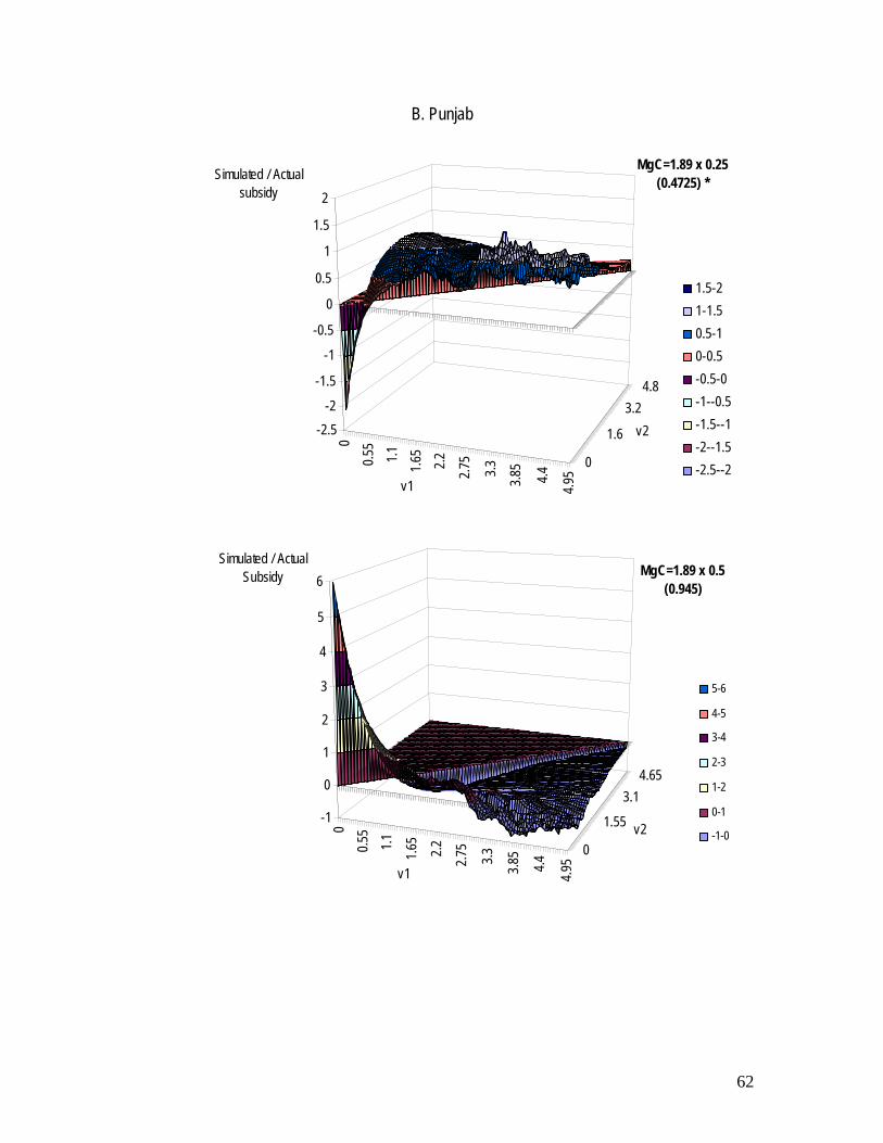
62
B. Punjab
00.5
51.1 1.6
52.2 2.7
5
3.3 3.85
4.4
4.95
0
1.6
3.24.8
-2.5-2
-1.5
-1
-0.5
0
0.5
1
1.5
2Simulated / Actual
subsidy
v1
v2
1.5-21-1.50.5-10-0.5-0.5-0-1--0.5-1.5--1-2--1.5-2.5--2
MgC=1.89 x 0.25(0.4725) *
00.5
51.1 1.6
5
2.2 2.75
3.3 3.85
4.4 4.95
0
1.55
3.14.65
-1
0
1
2
3
4
5
6Simulated / Actual
Subsidy
v1
v2
5-6
4-5
3-4
2-3
1-2
0-1
-1-0
MgC=1.89 x 0.5(0.945)

63
00.5
51.1 1.6
5
2.2 2.75
3.3 3.85
4.4 4.95
0
1.55
3.14.65
0
0.5
1
1.5
2
2.5Simulated / Actual
subsidy
v1
v2
2-2.51.5-21-1.50.5-10-0.5
MgC=1.89 x 1.25(2.3625)
00.5
51.1 1.6
5
2.2 2.75
3.3 3.85
4.4 4.95
0
1.55
3.14.65
-0.5
0
0.5
1
1.5
2
2.5
3
3.5Simulated / Actual
Subsidy
v1
v2
3-3.5
2.5-3
2-2.5
1.5-2
1-1.5
0.5-1
MgC=1.89 x 0.75(1.4175)

64
00.5
51.1 1.6
5
2.2 2.75
3.3
3.85
4.4
4.95
0
1.6
3.24.8
0
0.5
1
1.5
2
2.5Simulated / Actual
Subsidy
v1
v2
2-2.51.5-21-1.50.5-10-0.5
MgC=1.89 x 1.5(2.835)
00.5
51.1 1.6
52.2 2.7
5
3.3
3.85
4.4
4.95
0
1.6
3.24.8
0
0.5
1
1.5
2
2.5Simulated / Actual
Subsidy
v1
v2
2-2.51.5-21-1.50.5-10-0.5
MgC=1.89 x 1.5(2.835)

65
To be able to do this we can differentiate with respect to f the previous ratio:
1 1 1
1 1
1 1
1 1 1
11 1 1
1.18 (1.18 ) 1.18 (1.18 )
= 0
=
but we know: and therefore:
=
T T T
T T
T T
T T T
T T TT
dR q fq R q fq Rdf
R q q Rq Rq R
R q P R q P
q q P P Pq q P
= − − −
− >
>
= =
> ⇒ >
Therefore the ratio will increase if the weighted average price faced by large and small holders is bigger than the price faced by the small holders (i.e. the first part tariff). This can be appreciated in Figure 5.6a and 5.6b, as the values of v1 and v2 increase, i.e. PT is bigger than P1, and f increases, the subsidy to small holders will increase. To simplify, in Figure 5.6a and 5.6b we have fixed the values of v1 and v2 and simulated what will be the ratio as we increase the marginal cost. As can be seen in the case of AP, when the marginal cost increases from 0.295 to 0.885, there is a significant increase in the ratio, i.e. the subsidies are more progressive. Although when the marginal cost is higher than our initial estimate of 1.18 ruppies per kwh, the share of small holder subsidy over the total subsidy reduces 87% and to 79.8% for a marginal cost of 1.475 and 2.065 respectively. Similar results hold for the case of Punjab.

66
Figure 4.6 Impact of Changes in Tariff Schedule on Share of Smallholders in Total Subsidy, under Different Assumptions
of Marginal Cost (v1<v2)
Andhra Pradesh
0.5
1.2
1.9
2.6
3.3 4
4.7
0.55
2.55
4.55
0
0.1
0.2
0.3
0.4
0.5
0.6Share
v 1
v 2
0.5-0.6
0.4-0.5
0.3-0.4
0.2-0.3
0.1-0.2
0-0.1
MgC=1.18 x 0.25(0.295) *
v1=2.5; v2=3.5Share=22.7%
0
0.8
1.6
2.4
3.2 4
4.8
0
2.25
4.5
0
0.5
1
1.5
2
2.5
3Share
v 1
v 2
2.5-3
2-2.5
1.5-2
1-1.5
0.5-1
0-0.5
MgC=1.18 x 0.75(0.885)
v1=2.5; v2=3.5Share=126.7%
0
0.8
1.6
2.4
3.2 4
4.8
0
2.25
4.5
0
0.2
0.4
0.6
0.8
1Share
v 1
v 2
0.8-1
0.6-0.8
0.4-0.6
0.2-0.4
0-0.2
MgC=1.18 x 1.25(1.475)
v1=2.5; v2=3.5Share=87.0%
0
0.8
1.6
2.4
3.2 4
4.8
0
2.25
4.5
0
0.2
0.4
0.6
0.8
1Share
v 1
v 2
0.8-1
0.6-0.8
0.4-0.6
0.2-0.4
0-0.2
MgC=1.18 x 1.75(2.065)
v1=2.5; v2=3.5Share=79.8%
* Due to outlier values, only results for v1>0.05 and v2>0.05 are reported.

67
Punjab
0.55
1.15
1.75
2.35
2.95
3.55
4.15
4.75
0.55
2.2
3.85
0
0.1
0.2
0.3
0.4
0.5
0.6
0.7
0.6-0.7
0.5-0.6
0.4-0.5
0.3-0.4
0.2-0.3
0.1-0.2
0-0.1
MgC=1.89 x 0.25(0.4725) *
v1=1.5; v2=2.5Share=14.1%
0
0.65 1.3
1.95 2.6
3.25 3.9
4.55
0
1.85
3.7
00.10.20.30.4
0.5
0.6
0.7
0.8
0.9
0.8-0.9
0.7-0.8
0.6-0.7
0.5-0.6
0.4-0.5
0.3-0.4
0.2-0.3
0.1-0.2
0-0.1
MgC=1.89 x 0.75(1.4175)
v1=1.5; v2=2.5Share=38.8%
0
0.7
1.4
2.1
2.8
3.5
4.2
4.9
0
1.9
3.8
00.10.20.30.40.5
0.6
0.7
0.8
0.9
0.8-0.9
0.7-0.8
0.6-0.7
0.5-0.6
0.4-0.5
0.3-0.4
0.2-0.3
0.1-0.2
0-0.1
MgC=1.89 x 1.25(2.3625)
v1=1.5; v2=2.5Share=20.8%
0
0.7
1.4
2.1
2.8
3.5
4.2
4.9
0
1.9
3.8
00.10.20.30.40.5
0.6
0.7
0.8
0.9
0.8-0.9
0.7-0.8
0.6-0.7
0.5-0.6
0.4-0.5
0.3-0.4
0.2-0.3
0.1-0.2
0-0.1
MgC=1.89 x 1.75(3.3075)
v1=1.5; v2=2.5Share=19.5%
* Due to outlier values, only results for v1>0.05 and v2>0.05 are reported.

68
4.5 Simulating impacts of an optimal consumption plan with a variable first part and two marginal rates – Simulation 3
Simulation 2 allowed us to introduce a fixed rate (F) and two variable components in the tariff schedule. Different combinations of v1 and v2 yielded various outcomes. Nevertheless, assuming a marginal cost of 1.18 and 1.89 for Andhra Pradesh and Punjab, respectively, no combination of v1 and v2 resulted in positive profits for the electricity firm. In this sense, a new simulation introducing variable parameters (v1, v2) and increases of the fixed rate are introduced. While increases in fixed rates may allow for cuts in the electricity subsidy, it may also reduce the subsidy in the first segment of the tariff schedule (66% and 44% in Andhra Pradesh and Punjab, respectively).
While most of the assumptions and methodological issues of Simulation 2 are kept, variation of the fixed rate has been allowed. Thus, impact on profit of different combinations of F, v1 and v2 are analyzed altogether. Range for v1 and v2 is kept [0, 5] (v1<v2), while variations of F are assumed as a percentage of fixed rates assumed in simulation 2 (337.5 and 810 in Andhra Pradesh and Punjab, respectively). We have tested increases of 25%, 50%, 75%, 100%, 125%, and 150% on the original values of the fixed rate. Results are reported in Figure 4.7a and 4.7b. The higher the level of the first part of the tariff, the more the small holders will pay for the service and therefore the smaller the level of the subsidy for the first part of the tariff. This proposed mechanism could be optimal if farmers are allowed to assign themselves to different pricing schemes (consumer plans). This is similar to what we currently observe in cellular phones and is a way how farmers could self select themselves to a specific plan taking into account their own differences in consumption patterns. Farmers with the smaller plots will normally need a small amount of electricity and therefore their major cost is the fixed monthly rent. A consumption plan featuring a low monthly fixed tariff and higher charges for additional kwh of consumption would improve the welfare of low-income farmer. The opposite is true in the case of rich farmers, whose major gain in welfare is through the intensive use of electricity to irrigate their plots. The welfare of this farmer would increase if the variable tariffs (v1 and v2) were reduced while the fixed monthly tariff was increased. In either case, the central objective of not breaking the equilibrium in the tariffs must be maintained to avoid the vicious circle mentioned in Chapter 2.
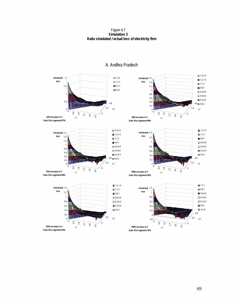
69
Figure 4.7 Simulation 3
Ratio simulated / actual loss of electricity firm
A. Andhra Pradesh
0
0.9
1.8
2.7
3.6
4.5
0
2.4
4.8
0
0.5
1
1.5
2sim/actual loss
v 1
v 2
25% increase in FSubs first segment=57%
1.5-2
1-1.5
0.5-1
0-0.5
0
0.9
1.8
2.7
3.6
4.5
0
2.4
4.8
00.20.40.60.8
1
1.2
1.4
1.6sim/actual loss
v 1
v 2
50% increase in FSubs first segment=49%
1.4-1.6
1.2-1.4
1-1.2
0.8-1
0.6-0.8
0.4-0.6
0.2-0.4
0-0.2
0
0.9
1.8
2.7
3.6
4.5
0
2.4
4.8
00.20.40.60.8
1
1.2
1.4
1.6sim/actual loss
v 1
v 2
75% increase in FSubs first segment=40%
1.4-1.6
1.2-1.4
1-1.2
0.8-1
0.6-0.8
0.4-0.6
0.2-0.4
0-0.2
0
0.9
1.8
2.7
3.6
4.5
0
2.4
4.8
0
0.2
0.4
0.6
0.8
1
1.2
1.4sim/actual loss
v 1
v 2
100% increase in FSubs first segment=32%
1.2-1.4
1-1.2
0.8-1
0.6-0.8
0.4-0.6
0.2-0.4
0-0.2
0
0.9
1.8
2.7
3.6
4.5
0
2.50
0.2
0.4
0.6
0.8
1
1.2
1.4sim/actual loss
v 1
v 2
125% increase in FSubs first segment=23%
1.2-1.4
1-1.2
0.8-1
0.6-0.8
0.4-0.6
0.2-0.4
0-0.2
0
0.9
1.8
2.7
3.6
4.5
0
2.4
4.8
-0.2
0
0.2
0.4
0.6
0.8
1
1.2sim/actual loss
v 1
v 2
150% increase in FSubs first segment=15%
1-1.2
0.8-1
0.6-0.8
0.4-0.6
0.2-0.4
0-0.2
-0.2-0y

70
B. Punjab
0
0.9
1.8
2.7
3.6
4.5
0
2.4
4.8
0
0.5
1
1.5
2
2.5sim/actual loss
v 1
v 2
25% increase in FSubs first segment=30%
2-2.5
1.5-2
1-1.5
0.5-1
0-0.5
0
0.9
1.8
2.7
3.6
4.5
0
2.4
4.8
-0.5
0
0.5
1
1.5
2
2.5sim/actual loss
v 1
v 2
50% increase in FSubs first segment=16%
2-2.5
1.5-2
1-1.5
0.5-1
0-0.5
-0.5-0
0
0.9
1.8
2.7
3.6
4.5
0
2.4
4.8
-0.5
0
0.5
1
1.5
2
2.5sim/actual loss
v 1
v 2
75% increase in FSubs first segment=2%
2-2.5
1.5-2
1-1.5
0.5-1
0-0.5
-0.5-0
0
0.9
1.8
2.7
3.6
4.5
0
2.4
4.8
-0.5
0
0.5
1
1.5
2sim/actual loss
v 1
v 2
100% increase in FSubs first segment= -11%
1.5-2
1-1.5
0.5-1
0-0.5
-0.5-0
0
0.9
1.8
2.7
3.6
4.5
0
2.4
4.8
-0.5
0
0.5
1
1.5
2sim/actual loss
v 1
v 2
125% increase in FSubs first segment= -25%
1.5-2
1-1.5
0.5-1
0-0.5
-0.5-0
0
0.9
1.8
2.7
3.6
4.5
0
2.4
4.8
-0.5
0
0.5
1
1.5
2sim/actual loss
v 1
v 2
150% increase in FSubs first segment= -39%
1.5-2
1-1.5
0.5-1
0-0.5
-0.5-0

71
4.6. Metering as a Necessary Condition and the alternative of Pre-paid Meters Although the proposed tariff schemes can be implemented based on the simulated electricity consumption by the farmers according to their plot size and what they produce, this could end in significant errors and won’t capture the changes in consumption patterns after the tariffs schemes are put into practice. Therefore, one major requirement to correctly implement the above pricing schemes is the knowledge of how much electricity is consumed by each type of farmer, i.e. the existence of metering devices. However, the traditional method of electricity distribution and interconnection to the main network is often unfeasible or not cost efficient in isolated rural areas. Moreover, due to the difficulties involved with traditional electric systems such as high transportation costs for payments and bill collection, the risk of using electricity indiscriminately, and the potential for power cuts and indebtedness form payment failure, an innovate strategy of prepaid meters could be implemented. With the prepaid meter system, clients buy a certain amount of electricity and are given a digital code which they punch into their meter and are immediately provided electricity. Currently this is being implemented in other countries with significant success (in Canada and Peru, for example). As a result, farmers will be able to control their energy consumption, they can buy electricity in small amounts and there is no minimum monthly fee like traditional electric systems. In addition consumers cannot develop a debt which gains interest since it is a fee for service system. Furthermore reconnection costs are near zero. One additional advantage of this system is that given it is based in a code system, this will also allow to better target the subsidy to specific farmer groups. In that sense subsidized cards can be directly assigned allowing for perfect targeting of the subsidy.
72
5. Conclusions The use of electricity in agriculture for irrigation following the green revolution has significantly contributed to agricultural productivity growth in India. There are two main sources of irrigation in India, one is canal water and the other is tube well irrigation using fuel or electric pumps. Even though, most of the change between 1960 and 2000 came mostly from tube well irrigation. Irrigated area under canal irrigation moved from 104 lakh in 1960 ha to 160 lakh ha in 2000, while tube well irrigation increase from 1 lakh ha to 217 lakh ha for the same years. With the increased role of tube well irrigation, the energization of tube well took place in a rapid pace. However, there is an inbuilt inefficiency in the current pricing mechanism and measuring system of power for irrigation in India and specifically in Andhra Pradesh and Punjab. This inbuilt inefficiency which essentially consist that, the cost of electricity for irrigation for majority of the farmers is fixed per month based on pump capacity and under the real marginal cost. As a result farmers incur almost a zero cost for irrigation in the short-run resulting in a pervasive incentive to overuse electricity and water ending in a strong mismatch between consumption share and revenue share. Though there were improvements in few states after the initiation of power sector reforms in the late 90s, the overall scenario has remained relatively unchanged and had worsen in the last year and the consequences had reached critical levels. This permanent mismatch between agricultural consumption of electricity and revenue from agriculture has created severe imbalances. All these have resulted in a higher gross subsidy per unit (Kwh) of energy sold. In 2001-02, the gross subsidy stood at 127 paise/Kwh, which was more than one-third of the cost of electricity supply. In absolute term, the total commercial losses of the SEBs (without subsidy) increased from Rs.113.1 billion in 1995-96 to Rs.331.8 billion in 2000-01. In terms of rate of return (ROR), this represents deterioration from –12.7% in 1992-93 to –44.1% in 2001-02 (GOI 2002a). In addition, the subsidy is benefiting mostly the large farmers. For instance, in the case of Punjab, the richest 10% receive around 41% of total subsidy while the poorest 10% receive 0.4% of total subsidy. One of the mechanisms used to cover the subsidy for agricultural (and domestic) power consumption was cross-subsidy from industrial and commercial consumers. In fact, the tariff charged to industrial and commercial consumers in India has been one of the highest in the world. As expected, this high-tariff for industry and high-subsidy for agriculture had two opposing effects on these two sectors: first, industry opted to substitute the power from public grid by resorting to captive generation reducing the potential cross-subsidy for agriculture; and second, a perverse incentive scheme generated an electricity consumption boom in agriculture. For AP and Punjab, the internal subsidy from the industrial sector could cover around 41% and 29%, respectively. In addition to this shortfall, the gap between cross-subsidy generated and subsidy needed has been increasing since the rate of growth in cross-
73
subsidy has been lagging firmly behind the rate of growth in agricultural subsidy. As a result, in 2001-02, the total cross-subsidy was sufficient enough to cover only around 21% of subsidy needed in agriculture. In AP and Punjab, it could cover only around 19% and 14%, respectively (GOI 2002a). Linked to the pricing mechanism is the measurement problem that breeds inefficiency and corruption. At present, there is no accurate estimate of actual power consumption in agriculture. Currently it is measured as a residual consumption after deducting non-agricultural consumption, and technical losses from total production. However, the current measurement has in-built incentives for corruption and by passing technical losses, inefficiencies, and consumption in other sectors under the name of agricultural consumption. If actual consumption is known, public authorities can decide on financing needs and financing methods and can also implement price strategies as the ones recommended in this report. Both of this problems have generated what we called along this report a vicious cycle which results in poor supply outcome in form of low quality of power, unreliable supply, unavailable to many potential users and high transmission and distribution (T&D) losses. In addition it had exacerbated the fall of the ground water level. In the case of Andhra Pradesh all the blocks has experienced a fall on the ground water level bigger than 4 meters since 1984. There has been an annual fall of 20cms per year. In the case of Punjab 4/5 of the blocks are also under four meters since 1984, 52.17% of the total blocks in the state are over-exploited and 7.97% of all blocks are ‘dark’ areas as on 31-3-98 (GOI, 2002b) and are also considered over exploited, i.e. the net recharge is substantially negative. It is obvious from the above discussions that the power reforms in India in general have largely ignored the reforms in power supply to agriculture. However, this is where the reform is needed most. The objective of this research was to identify a possible solution to the current vicious circle and if possible to turn it into a virtuous circle as shown in Figure 6.1 under two major premises: minimizing the impact of price changes over small holders and charging at least marginal cost to high demanders. In addition the proposed solution consists of a sequence of stages in such a way that its implementation could be politically feasible. A price discrimination strategy is proposed based on the size of the farmers plot and on the implementation of a two part tariff mechanism. Specifically three types of consumers are identified, small holders (more than zero ha and less or equal to 1.8 ha), medium holders (more than 1.8 ha and less or equal than 3.64 ha) and large holders (more than 3.64 ha) and a common two part tariff is proposed. In the first stage we propose that within the two part tariff the first part of the tariff will be equivalent to the value of the average current consumption of the small holders, which will, at the same time, be the amount of the subsidy. This will assure that on the one hand, the small holders will on average not be affected by this new price mechanism, and on the other hand, the subsidy will be better targeted. The second part of the tariff will be

74
set at levels higher than the marginal cost in such a way that high demanders will cover their costs and if possible cross subsidize the small holders. The result of this first stage are that for Andhra Pradesh small holders continue to consume the same amount of electricity at the same price; medium holders reduce their consumption by 14% and their weighted price (combinations of the first and second part of the tariff weighted by the quantity consumed in each part) increases by 25.1%; and finally, large holders reduce their consumption by 41% and their weighted price increases by 82.2%. In the case of Punjab small holders continue to consume the same amount of electricity at the same price; medium holders reduce their consumption by 16% and their weighted price increases by 17.1%; and finally, large holders reduce their consumption by 47% and their weighted price increases by 55.3%. This new price schedule assures that the subsidy is distributed in a more progressive way in contrary to what currently happens, i.e. the richest households in rural areas who reap most of the benefits of irrigation subsidy The second stage consists of a price scheme designed to significantly improve the progressiveness of the distribution of the subsidy with respect to the first two part tariff mechanism. In addition, this new pricing mechanism has the objective to reduce (not to eliminate) the burden of the subsidy to the government by cross subsidizing small holders with the revenues from large holders. This second mechanism considers a fixed rate (F), under which the household receives q1 units of electricity. Consumption exceeding q1 is charged with a marginal cost v1 for households demanding less than q2 units, and households with consumption exceeding q2 will pay v2 for additional units. Similarly, and with the same logic of the first tariff scheme, the fix rate (F) is calculated as the average consumption and expenditure of small holders so that they will not be affected by this new price scheme. In the case of Andhra Pradesh with tariffs of v1=2 ruppies per kwh and v2=3.45 ruppies per kwh the subsidy can be reduced to 33% of the current subsidy and large holders will cross subsidize small holders reducing significantly the burden of the government. In the case of Punjab the prices of v1 and v2 will have to be 4.9 and 5 to be able to arrive to a similar scenario as Andhra Pradesh. This is so because the land ownership is far more concentrated in Punjab than in Andhra Pradesh and therefore under the current situation the subsidies are clearly benefiting a lot more the large holders. In addition, we have simulated the impacts under different scenarios of marginal costs. Finally, the third stage proposes a pricing mechanism in which we try to completely eliminate the burden of the subsidy to the government. To be able to implement this mechanism, not only a new simulation introducing variable parameters (v1 and v2) as in the previous tariff schedule is kept, but also raises of the fixed rate are introduced. While increases in fixed rates may allow for reductions in the electricity subsidy, it may also reduce the subsidy for the small holders (i.e. 66% and 44% in Andhra Pradesh and Punjab, respectively) therefore this is a decision to be made by the government. In summary, in all these three price schemes, the major result is that the subsidy will be more progressive and resources will be used more efficiently. If low-demand consumers

75
or high-demand consumers want to consume more electricity, they will need to pay a charge over the marginal costs for each unit above their fixed charge. Finally, one major caveat is that although any of these price schemes can be implemented based on existing information, the ideal situation would be to be able to move to gradual elimination of the subsidies (i.e. from price scheme 1 to scheme 3), there is a clear need to develop better mechanisms to measure consumption and consumption patterns of households. With this respect the use of pre-paid meters will be an ideal solution to better implement the alternative pricing mechanisms. The identification of farmers will allow to a better allocation of subsidies on poorer farmers. The resources for this subsidy should not be higher than the total amount that can be collected from other consumer groups. In conclusion, these recommendations, which can also be implemented with canal water provision, could open an alternative to move from a vicious circle, in which the environmental situation will substantially worsen and the capacity of generation of electricity will be seriously damaged, to a virtuous circle, where the subsidy is assigned in a more progressive way, the trend in reduction of underground water is overturned and the electric providers can have sufficient resources to improve the quality of the electricity supplied.

76
References Andrikopoulos, A., and J. Loizides. 2000. The demand for home-produced and imported
alcoholic beverages in Cyprus: the AIDS approach. Applied Economics 32 (9): 1111-1119
AP Government. Vision 2020 http://www.apinfrastructure.com/vision2020.html Backer, P., Blundell, R., and Micklewright, J. 1989. Modelling Household Energy
Expenditures Using Micro-Data. Economic Journal, 99 (397): 720-738. Benjamin, Dwayne. 1992. “Household Composition, Labor Markets, and Labor Demand:
Testing for Separation in Agricultural Household Models”; Econometrica, Vol 60, No.2, pp.287-322.
Bose, Ranjan Kumar and Shukla, Megha. 1999. ”Elasticies of Electricity Demand in India”, Energy Policy 27(1999) p.137-146,
Deaton, Angus, and John Muellbauer. 1980. An Almost Ideal Demand System. American Economic Review, 70(3): 312-326.
Dhar, Tirtha, Jean-Paul Chavas, Brian W Gould. 2003. An Empirical Assessment of Endogeneity Issues in Demand Analysis for Differentiated Products. American Journal of Agricultural Economics 85 (3): 605-617
Directorate of Economics and Statistics, Andhra Pradesh, http://www.ap.gov.in/apbudget Dixit, Shantanu, Girish Sant and Subodh Wagle 1998. Regulation in the WB-Orissa
Model: Cure Worse Than Disease, ’Economic And Political Weekly, XXXIII (17) April 25.
Expert Group. 2003. Power Reforms in Punjab. New Delhi: National Council of Applied Economic Research.
GOI. 1992. Viadyanathan Committee Report. Source: http://www.fiscalconf.org/papers/vaidya.pdf, access date: June 3, 2004.
GOI. 2002. National Water Policy 2002. Ministry of Water Resources. http://wrmin.nic.in/policy/nwp2002.pdf, access date: June 7, 2004.
Government of India. 2002. Annual Report on the Working of State Electricity Boards and Electricity Departments, Power and Energy Division, Planning Commission
Government of India. 2002b. Tenth Five-Year Plan, 2002-07. Volume II, Planning Commission, Government of India.
Gulati, A. 1999. Pricing for Power and Water for Irrigation: Issues Related to Efficiency and Stustainability. Mimeo. November.
Gulati, A. and S. Narayanan. 2003. The Subsidy Syndrome in Indian Agriculture. New Delhi: Oxford University Press.
Hira, G.S. and K.L. Khera. 2000. Water Resource Management in Punjab under Rice-Wheat Production System. Research Bull. No.2. Dept. of Soils. Punjab Agricultural University. Ludhiana.
IDFC. 1998. Power Sector in India: A Summary Description. Infrastructure Development Finance Company Limited (IDFC). New Delhi.
Indiastat. Indiastat.com (an online data source on India) Kaur, R. 2003. Rationalization of Input Subsidies in Punjab, India. Unpublished
Manuscript. Washington, DC: IFPRI

77
Larson, Donald W., Eugene Jones, R.S. Pannu, and R.S. Sheokand. 2004. Instability in Indian Agriculture – a challenge to the Green Revolution Technology. Food Policy, 29 (3): 257-273.
Mazzocchi, M. 2003. Time-varying coefficients in the Almost Ideal Demand System: an empirical appraisal, European Review of Agricultural Economics 30(2): 241-270
Ministry of Water Resources, GOI, http://wrmin.nic.in/development/status_deve.htm, access date: May 6, 2004.
Nicol, C.J. Estimating a Third-Order Translog Using Canadian Cross-Sectional Micro-Data. Canadian Journal of Economics, 22(5): 543-560.
NSSO (National Sample Survey Organization). 2000. Household Consumer Expenditure in India 1999-2000 Key Results. Report No. 454 (55/1.0/2). National Sample Survey Organization, Ministry of Statistics and Programme Implementation, Government of India.
Pollak, R.A., and T.J. Wales. 1980. A Comparison of the Quadratic Expenditure System and the Translog Demand System with Alternative Specifications of Demographic Effects. Econometrica 48, 595-612.
Pollak, R.A., and T.J. Wales. 1981. Demographic Variables in Demand Analysis. Econometrica 49, 1533-51.
Power Ministry 2004. http://powermin.nic.in/note2003.htm, access date: April 26, 2004 Price Water House Coopers. Infrastructure Development Action Plan for Chhattisgarh –
Final Report (http://chhattisgarh.nic.in/opportunities/Annexure%203.2.pdf, access date: August 31, 2004).
Punjab Government. Budget Speech for the year 2003-04, Finance Minister of Punjab, http://www.punjabgov.net, access date: May 10, 2004
Punjab Government. http://www.punjabenvironment.com/status.htm, access date: May 10, 2004.
Punjab State Electricity Regulatory Commission (PSERC). Tariff Order 2003. Chandigarh.
Raju, and Gulati 2002 Raju, KV. 2000. Participatory Irrigation Management in Andhra Pradesh: Promise,
Practice and a Way Forward. Working Paper 65, Institute of Social Studies, Bangalore.
Ray, Ranjan. 1980. Analysis of a Time Series of Household Expenditure Surveys for India. Review of Economics and Statistics, 62 (4): 595-602.
Reddy, R. 2003. Irrigation: Development and Reforms. in: Rao, CHH., and Dev, M. (eds.) Andhra Pradesh Development: Economic Reforms and Challenges Ahead. pp. 170-201. Hyderabad: Centre for Economic and Social Studies.
Smith, Laurence E. D. 2004. Assessment of the Contribution of Irrigation to Poverty Reduction and Sustainable Livelihoods. Water Resources Development, 20(2): 243-257.
Song, H., Liu, X., and Romilly, P. 1997. A Comparative Study of Modelling the Demand for Food in the United States. Journal of Applied Economics, 12 (5): 593-608.
Stone, JRN. 1953. The Measurement of Consumers’ Behaviour in the United Kingdom, 1920-1938, Vol. 1. Cambridge.

78
Taylor, J.Edward and Adelman, Irma. 2003. “Agricultural Household Models: Genesis, Evolution, and Extensions”. In Review of Economics of the Household, Vol. 1, No.1.
Terri (The Energy and Resource Institute). 2003. Teri Energy Data Dictionary and
Yearbook 2002/03. New Delhi: Terri. Veeraiah, Ch. and N. Madankumar. 1994.Waste of Irrigation Water Under Major
Irrigation Projects in Andhra Pradesh and its Prevention, cited in Gulati and Narayanan 2003.
WDI 2004. World Development Indicators. Washington DC: World Bank. World Bank, 2001. India: Power Supply to Agriculture. Volume 1, Summary Report.
Energy Sector Unit, South Asia Regional Office. World Bank, 2003a. Why are power sector reforms important for the poor? New Delhi:
World Bank. World Bank. 2003b. The Incidence of Canal Irrigation Subsidies in India. South Asia
Rural Development Unit, World Bank. Xepapadeas, Anastasios, and Hassini Habib. 1995. An almost ideal demand system with
autoregressive disturbances for dairy products in Greece. Applied Economics Letters 2(6): 169-173
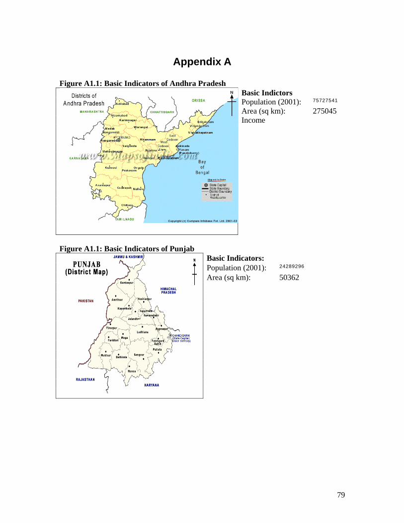
79
Appendix A Figure A1.1: Basic Indicators of Andhra Pradesh
Basic Indictors Population (2001): 75727541 Area (sq km): 275045 Income
Figure A1.1: Basic Indicators of Punjab
Basic Indicators: Population (2001): 24289296 Area (sq km): 50362
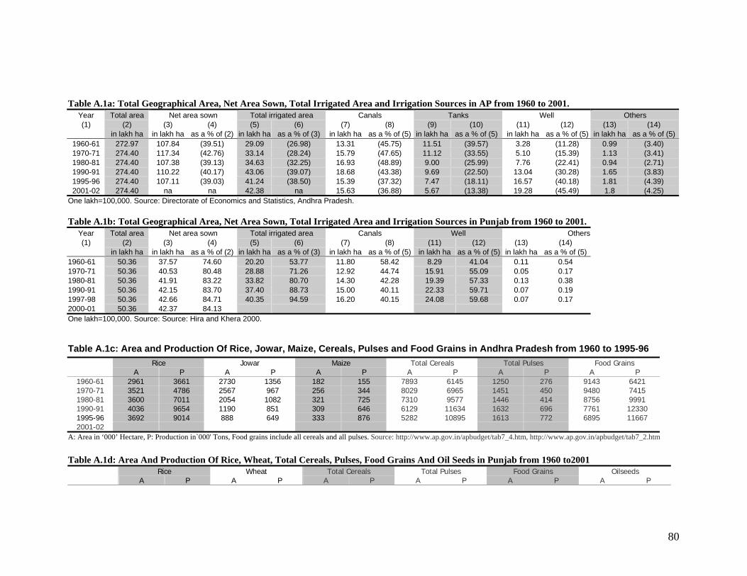
80
Table A.1a: Total Geographical Area, Net Area Sown, Total Irrigated Area and Irrigation Sources in AP from 1960 to 2001.
Year Total area Net area sown Total irrigated area Canals Tanks Well Others (1) (2) (3) (4) (5) (6) (7) (8) (9) (10) (11) (12) (13) (14)
in lakh ha in lakh ha as a % of (2) in lakh ha as a % of (3) in lakh ha as a % of (5) in lakh ha as a % of (5) in lakh ha as a % of (5) in lakh ha as a % of (5)1960-61 272.97 107.84 (39.51) 29.09 (26.98) 13.31 (45.75) 11.51 (39.57) 3.28 (11.28) 0.99 (3.40) 1970-71 274.40 117.34 (42.76) 33.14 (28.24) 15.79 (47.65) 11.12 (33.55) 5.10 (15.39) 1.13 (3.41) 1980-81 274.40 107.38 (39.13) 34.63 (32.25) 16.93 (48.89) 9.00 (25.99) 7.76 (22.41) 0.94 (2.71) 1990-91 274.40 110.22 (40.17) 43.06 (39.07) 18.68 (43.38) 9.69 (22.50) 13.04 (30.28) 1.65 (3.83) 1995-96 274.40 107.11 (39.03) 41.24 (38.50) 15.39 (37.32) 7.47 (18.11) 16.57 (40.18) 1.81 (4.39) 2001-02 274.40 na na 42.38 na 15.63 (36.88) 5.67 (13.38) 19.28 (45.49) 1.8 (4.25)
One lakh=100,000. Source: Directorate of Economics and Statistics, Andhra Pradesh. Table A.1b: Total Geographical Area, Net Area Sown, Total Irrigated Area and Irrigation Sources in Punjab from 1960 to 2001.
Year Total area Net area sown Total irrigated area Canals Well Others(1) (2) (3) (4) (5) (6) (7) (8) (11) (12) (13) (14)
in lakh ha in lakh ha as a % of (2) in lakh ha as a % of (3) in lakh ha as a % of (5) in lakh ha as a % of (5) in lakh ha as a % of (5)1960-61 50.36 37.57 74.60 20.20 53.77 11.80 58.42 8.29 41.04 0.11 0.54 1970-71 50.36 40.53 80.48 28.88 71.26 12.92 44.74 15.91 55.09 0.05 0.17 1980-81 50.36 41.91 83.22 33.82 80.70 14.30 42.28 19.39 57.33 0.13 0.38 1990-91 50.36 42.15 83.70 37.40 88.73 15.00 40.11 22.33 59.71 0.07 0.19 1997-98 50.36 42.66 84.71 40.35 94.59 16.20 40.15 24.08 59.68 0.07 0.17 2000-01 50.36 42.37 84.13 One lakh=100,000. Source: Source: Hira and Khera 2000.
Table A.1c: Area and Production Of Rice, Jowar, Maize, Cereals, Pulses and Food Grains in Andhra Pradesh from 1960 to 1995-96 Rice Jowar Maize Total Cereals Total Pulses Food Grains A P A P A P A P A P A P
1960-61 2961 3661 2730 1356 182 155 7893 6145 1250 276 9143 6421 1970-71 3521 4786 2567 967 256 344 8029 6965 1451 450 9480 7415 1980-81 3600 7011 2054 1082 321 725 7310 9577 1446 414 8756 9991 1990-91 4036 9654 1190 851 309 646 6129 11634 1632 696 7761 12330 1995-96 3692 9014 888 649 333 876 5282 10895 1613 772 6895 11667 2001-02
A: Area in ‘000’ Hectare, P: Production in`000' Tons, Food grains include all cereals and all pulses. Source: http://www.ap.gov.in/apbudget/tab7_4.htm, http://www.ap.gov.in/apbudget/tab7_2.htm Table A.1d: Area And Production Of Rice, Wheat, Total Cereals, Pulses, Food Grains And Oil Seeds in Punjab from 1960 to2001
Rice Wheat Total Cereals Total Pulses Food Grains Oilseeds A P A P A P A P A P A P
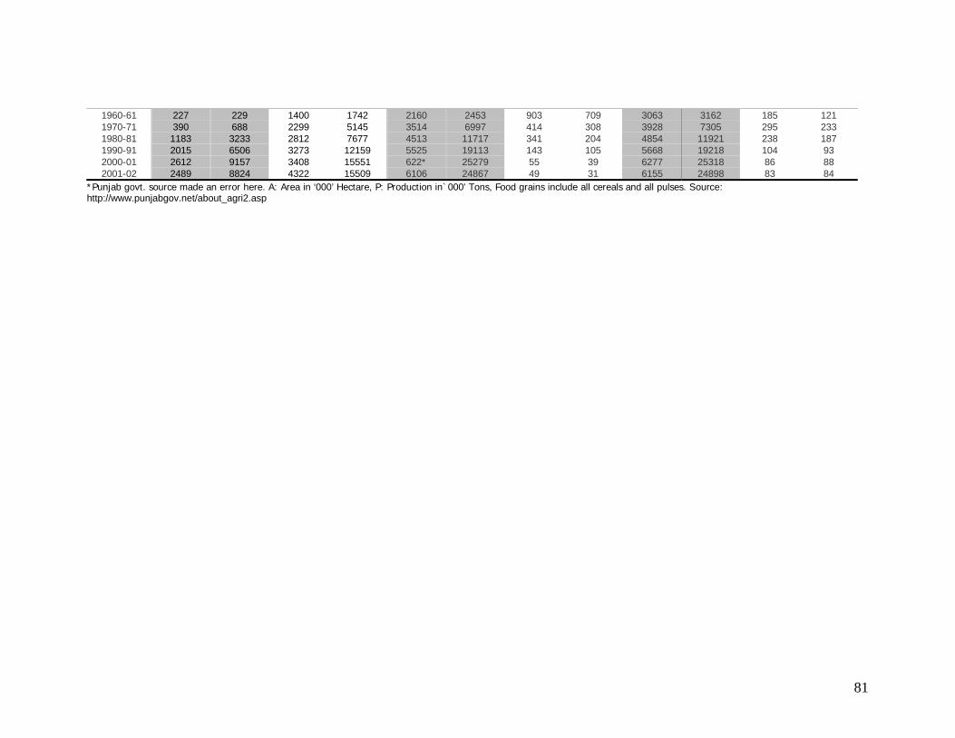
81
1960-61 227 229 1400 1742 2160 2453 903 709 3063 3162 185 121 1970-71 390 688 2299 5145 3514 6997 414 308 3928 7305 295 233 1980-81 1183 3233 2812 7677 4513 11717 341 204 4854 11921 238 187 1990-91 2015 6506 3273 12159 5525 19113 143 105 5668 19218 104 93 2000-01 2612 9157 3408 15551 622* 25279 55 39 6277 25318 86 88 2001-02 2489 8824 4322 15509 6106 24867 49 31 6155 24898 83 84
*Punjab govt. source made an error here. A: Area in ‘000’ Hectare, P: Production in`000' Tons, Food grains include all cereals and all pulses. Source: http://www.punjabgov.net/about_agri2.asp

11/8/2007 82
Table A.1e: Average Yields of Principal Corps (tons/ha): Irrigated vis-à-vis Non-irrigated Land Irrigated Non-irrigated 1971-72 1981-82 1991-92 1971-72 1981-82 1991-92 Food Crops 1.65 1.91 2.09 0.70 0.90 1.05 Paddy 2.40 2.77 3.18 1.04 1.54 1.08 Wheat 1.02 1.64 1.98 0.66 0.99 1.56 Maize Non-Food Crops 1.46 1.59 1.83 0.81 0.90 0.96 Groundnut 0.85 1.37 1.87 0.32 0.68 0.73 Cotton 41.41 58.37 63.84 37.47 41.33 46.87 Sugarcane
Source: (I need to find it out)
Figure A2.1a: Use of Electricity and Productivity, 1950-2000
0200400600800
10001200140016001800
0 100 200 300 400 500 600 700 800Consumption of Electricity (Kwh)/Hectare
Prod
uctio
n of
food
grai
ns
(Kg/
hect
are)
Data source: Terri 2003, GOI 2002.
Electricity Consumption and Agriculture Value Added in India, 1960-2001
0
10
20
30
40
50
0 5 10 15 20 25 30 35
Share of Agriculture in Electricity Consumption
Agr
icul
ture
Val
ue A
dded
(%
) of G
DP
Source: Terri 2003, GOI 2002, WDI 2004
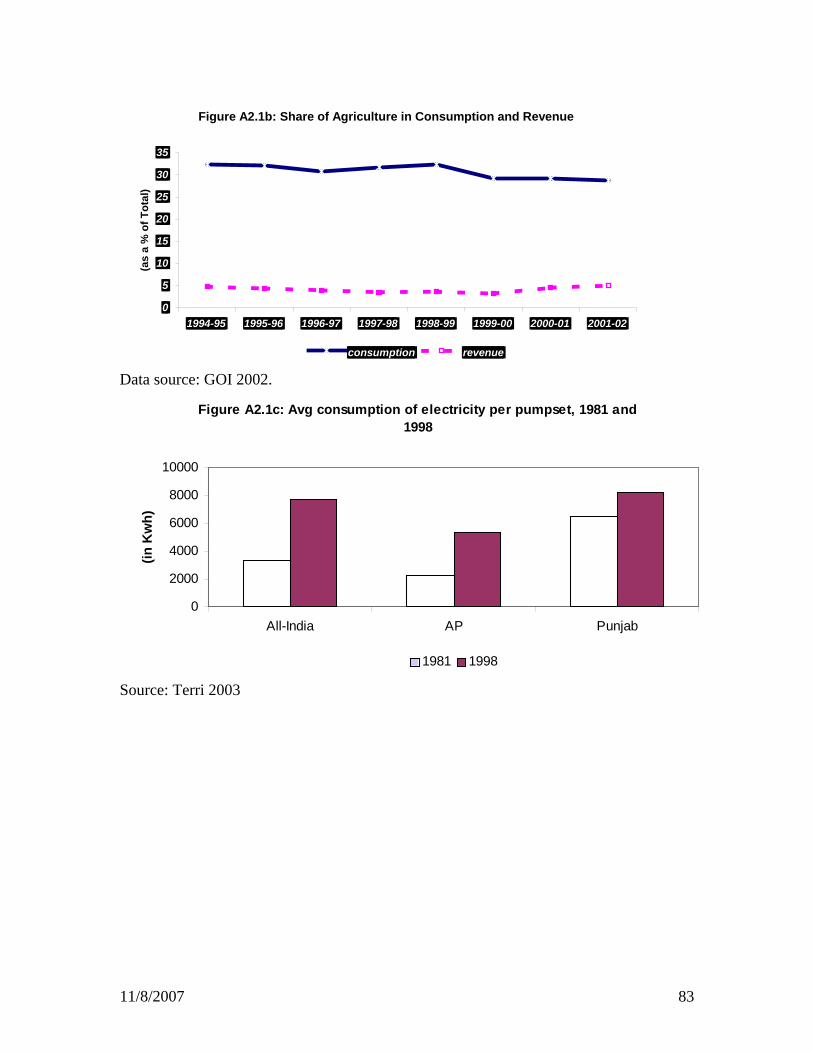
11/8/2007 83
Figure A2.1b: Share of Agriculture in Consumption and Revenue
0
5
10
15
20
25
30
35
1994-95 1995-96 1996-97 1997-98 1998-99 1999-00 2000-01 2001-02
(as
a %
of T
otal
)
consumption revenue
Data source: GOI 2002.
Figure A2.1c: Avg consumption of electricity per pumpset, 1981 and 1998
0
2000
4000
6000
8000
10000
All-India AP Punjab
(in K
wh)
1981 1998
Source: Terri 2003

11/8/2007 84
Figure A2.2: Annual commerical losses of the SEBs (Rs. Crore), 1990-2000
0
5000
10000
15000
20000
25000
30000
35000
40000
1990 1991 1992 1993 1994 1995 1996 1997 1998 1999 2000
(in c
rore
Rp.
)
Source: GOI 2002.
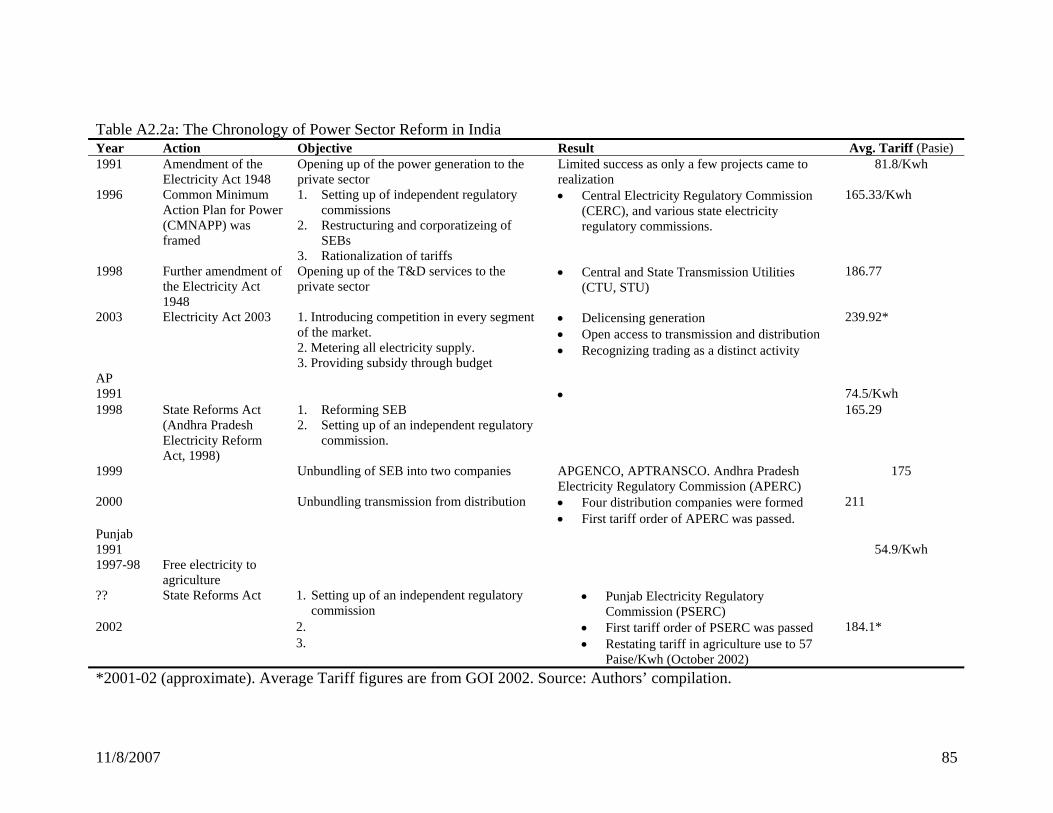
11/8/2007 85
Table A2.2a: The Chronology of Power Sector Reform in India Year Action Objective Result Avg. Tariff (Pasie) 1991 Amendment of the
Electricity Act 1948 Opening up of the power generation to the private sector
Limited success as only a few projects came to realization
81.8/Kwh
1996 Common Minimum Action Plan for Power (CMNAPP) was framed
1. Setting up of independent regulatory commissions
2. Restructuring and corporatizeing of SEBs
3. Rationalization of tariffs
• Central Electricity Regulatory Commission (CERC), and various state electricity regulatory commissions.
165.33/Kwh
1998 Further amendment of the Electricity Act 1948
Opening up of the T&D services to the private sector
• Central and State Transmission Utilities (CTU, STU)
186.77
2003 Electricity Act 2003 1. Introducing competition in every segment of the market. 2. Metering all electricity supply. 3. Providing subsidy through budget
• Delicensing generation • Open access to transmission and distribution • Recognizing trading as a distinct activity
239.92*
AP 1991 • 74.5/Kwh 1998 State Reforms Act
(Andhra Pradesh Electricity Reform Act, 1998)
1. Reforming SEB 2. Setting up of an independent regulatory
commission.
165.29
1999 Unbundling of SEB into two companies APGENCO, APTRANSCO. Andhra Pradesh Electricity Regulatory Commission (APERC)
175
2000 Unbundling transmission from distribution • Four distribution companies were formed • First tariff order of APERC was passed.
211
Punjab 1991 54.9/Kwh 1997-98 Free electricity to
agriculture
?? State Reforms Act 1. Setting up of an independent regulatory commission
• Punjab Electricity Regulatory Commission (PSERC)
2002 2. • First tariff order of PSERC was passed 184.1* 3. • Restating tariff in agriculture use to 57
Paise/Kwh (October 2002)
*2001-02 (approximate). Average Tariff figures are from GOI 2002. Source: Authors’ compilation.

11/8/2007 86
57081
27047
4139
62245
31606
11067
0%
20%
40%
60%
80%
100%
% o
f Ins
talle
d ca
paci
ty
1997 2002
Fig A2.2b: Reform and change in Ownership in Electricity Generation
State Central Private
Data source: GOI 2002
Figure A2.2c: Total Installed Capacity (in MW)
55136179
1059
3509
4529
0
1000
2000
3000
4000
5000
6000
7000
1997 2002 Private
MW
AP Punjab
31%
65%
5%
30%
59%
11%

11/8/2007 87
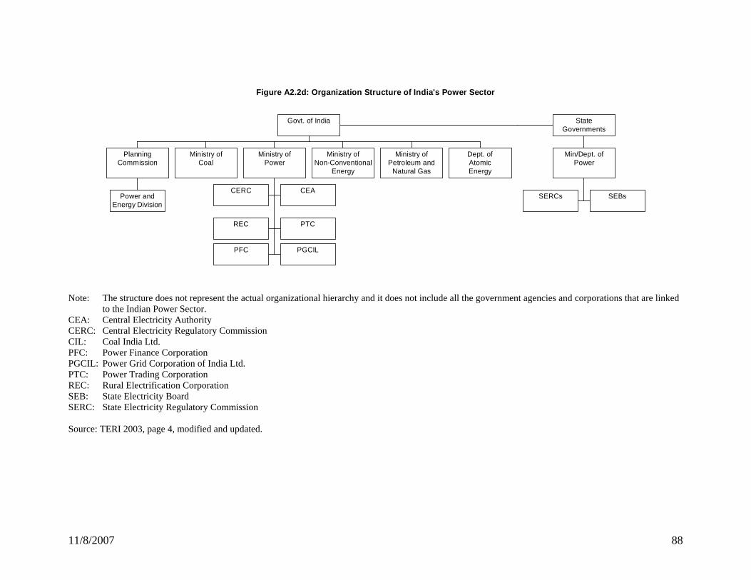
11/8/2007 88
Figure A2.2d: Organization Structure of India's Power Sector
Power andEnergy Division
PlanningCommission
Ministry ofCoal
CERC CEA
REC PTC
PFC PGCIL
Ministry ofPower
Ministry ofNon-Conventional
Energy
Ministry ofPetroleum and
Natural Gas
Dept. ofAtomicEnergy
Govt. of India
SERCs SEBs
Min/Dept. ofPower
StateGovernments
Note: The structure does not represent the actual organizational hierarchy and it does not include all the government agencies and corporations that are linked to the Indian Power Sector.
CEA: Central Electricity Authority CERC: Central Electricity Regulatory Commission CIL: Coal India Ltd. PFC: Power Finance Corporation PGCIL: Power Grid Corporation of India Ltd. PTC: Power Trading Corporation REC: Rural Electrification Corporation SEB: State Electricity Board SERC: State Electricity Regulatory Commission Source: TERI 2003, page 4, modified and updated.

11/8/2007 89
Table A2.3.1: Elasticity of electricity consumption with respect to GDP and agriculture GDP GDP Agricultural GDP Year Elasticity Year Elasticity First plan 1951-56 3.14 1970 17.00 Second plan 1956-61 3.38 1980 14.01 Third plan 1961-66 5.04 1985 3.60 Fourth plan 1969-74 1.85 1989 5.92 Fifth plan 1974-79 1.88 1990 3.46 Sixth plan 1980-85 1.39 1992 1.41 Seventh plan 1985-90 1.5 1993 2.82 Eighth plan 1992-97 0.97 1994 2.43 1998 0.76 Source: Calculated from Terri 2003, WDI 2004, GOI 2002 EEccoonnoommiicc SSuurrvveeyy,, MMiinniissttrryy ooff FFiinnaannccee,, EEccoonnoommiicc DDiivviissiioonn,, GGOOII,, 11999955--9966,, CCEEAA HHiigghhlliigghhttss,, CCEEAA,, 11999933--9944.. Notes: Due to year-to-year fluctuations in agricultural production, negative elasticity figures were dropped
Figure-A2.3.1: Share of Agriculture in Total Electricity Consumption
0
10
20
30
40
50
60
1992-93 1993-94 1994-95 1995-96 1996-97 1997-98 1998-99 1999-00 2000-01 2001-02
(in %
)
AP Punjab All India
Data source: GOI 2002

11/8/2007 90
Fig-A2.3.1b: Energization of Pump Sets as a % of Pump Sets Potential
60
70
80
90
100
110
1999 2000 2001 2002
(in %
)
All India AP Punjab
Data source: GOI 2002 Data source: Terri 2003
Fig-A2.3.1c: Consumption of Electricity: Per pump set and per capita in (Kwh)
0
2000
4000
6000
8000
10000
12000
1981 1986 1987 1993 1994 1995 1996 1997 1998
(in K
wh)
Pump-all India Pump-AP Pump-PJ per cap con
Notes: per cap con stands for per capita consumption of electricity. Source: Terri 2003, WDI 2004.
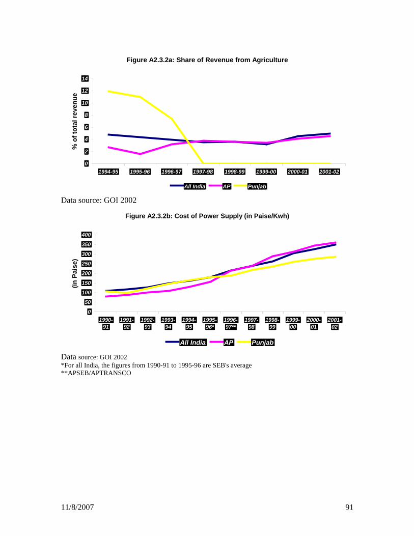
11/8/2007 91
Figure A2.3.2a: Share of Revenue from Agriculture
0
2
4
6
8
10
12
14
1994-95 1995-96 1996-97 1997-98 1998-99 1999-00 2000-01 2001-02
% o
f tot
al re
venu
e
All India AP Punjab
Data source: GOI 2002
Figure A2.3.2b: Cost of Power Supply (in Paise/Kwh)
0
50
100
150
200
250
300
350
400
1990-91
1991-92
1992-93
1993-94
1994-95
1995-96*
1996-97**
1997-98
1998-99
1999-00
2000-01
2001-02
(in P
aise
)
All India AP Punjab
Data source: GOI 2002 *For all India, the figures from 1990-91 to 1995-96 are SEB's average **APSEB/APTRANSCO

11/8/2007 92
Figure A2.3.2c: Cost of Power Supply and Average Tariff, AP and Punjab
50
100
150
200
250
300
350
400
1990-91 1991-92 1992-93 1993-94 1994-95 1995-96 1996-97 1997-98 1998-99 1999-00 2000-01 2001-02
(in P
aise
)
Cost-AP Avg. Tariff-AP Cost-Punjab Avg. Tariff-Punjab
Data source: GOI 2002.

11/8/2007 93
Figure A2.3.2d: Electricity prices for Industry in 2000 (US Dollars per Kilowatthour)
0.000.010.020.030.040.050.060.070.080.09
Russia SouthAfrica
Indonesia China USA OECD UK Thailand India
US
Dol
lars
Notes: For China and Indonesia, the tariff is for 1996 and 1999, respectively Energy end-use prices including taxes, converted using exchange rates. ��HOECD stands for Organization for Economic Cooperation and Development. Electricity prices in the United States include income taxes, environmental charges, and other charges. However, the prices excude the taxes collected for the convenience of the States and "passed through" to the customer. Source: http://www.eia.doe.gov/emeu/international/elecprii.html, access date: May 14, 2004.
Fig: 2A3.3e: Subsidy needed and Cross-subsidy generated
0
5000
10000
15000
20000
25000
30000
35000
40000
45000
1992-93 1993-94 1994-95 1995-96 1996-97 1997-98 1998-99 1999-00 2000-01 2001-02
(in c
rore
Rp.
)
Subsidy to agriculture and domestic sector Cross-subsidy from other sectors
Source: GOI 2002 Table A3a: AP's Budget Data: Actual Expenditure (in million rupees)
Major and medium Minor Total 1994-95 10792 907 11699 1995-96 10263 1033 11295 1996-97 10702 794 11496 1997-98 11717 1243 12960 1998-99 14388 1863 16251

11/8/2007 94
1999-00 13387 1348 14735 Source: Reddy 2003 Table A3b: Capacity of Canals in Punjab Name of Head Works Name of off-taking channels Capacity Ropar Headworks Ropar i) Sirhind Canal 12622 Cs. ii) Bist Doab Canal 1408 Cs Harike Headworks, Harike i) Rajasthan Feeder 18500 Cs. ii) Ferozepur Feeder 11192 Cs. iii) Mukhu Canal 292 Cs. Hussainiwala Headworks Ferozepur i) Bikaner Canal 2740 Cs. ii) Eastern Canal 3929 Cs. Madhopur Head Works i) Upper Bari Doab Canal 8200 Cs. Shah Nehar Headworks ii) Mukerjan Hydel Canal 11500 Cs Nangal Head works i) Bhakra Mainline Canal 12455 Cs. Source: Water Resources & Environment DTE. Irrigation Department,Punjab(Study Period 1995-97) Table A3c: Estimates of Irrigation Subsidy at all-India level. (In million Rs.)
Year Government Estimates
Vaidyanathan Committee method
O&M method
1981-82 6360 4578 2996 1982-83 7420 5424 3589 1983-84 7930 6320 4173 1984-85 10800 7255 4724 1985-86 11440 7440 4656 1986-87 15200 10779 7682 1987-88 16280 19715 16234 1988-89 22300 23544 19588 1989-90 24390 23088 18547 1990-91 24680 25713 20828 1991-92 31470 28681 23429 1992-93 34890 32876 27220 1993-94 39490 34414 28296 1994-95 45790 39542 32889 1995-96 53990 44118 36894 1996-97 62750 44394 36290 1997-98 70940 46557 38692 1998-99 82290 49367 41093 1999-00 87580 52177 43495
Source: Government Estimates from the National Accounts Statistics (various years). Other estimates from Gulati and Narayanan, 2003. Table A3d: Irrigation Subsidy in Punjab- O&M Approach (Rs. In million)
Year Irrigation Subsidy (at current prices) Irrigation Subsidy (at constant prices) 1981-82=100 1981-82 43.50 43.50 1982-83 34.00 32.41 1983-84 89.10 78.99 1984-85 31.00 25.81 1985-86 113.80 90.75 1986-87 108.70 81.91 1987-88 166.70 116.09 1988-89 167.10 108.30 1989-90 258.70 156.13 1990-91 221.70 121.35 1991-92 273.14 131.44 1992-93 307.08 134.27 1993-94 308.21 124.38 1994-95 236.51 84.76 1995-96 329.69 109.41 1996-97 482.84 153.18 1997-98 795.62 241.77 1998-99 873.77 250.61 1999-00 1259.50 349.81

11/8/2007 95
2000-01 1190.47 308.55 2001-02 1389.63 347.67
Source: Department of Irrigation, Punjab and Bhalla & Singh, 1996 (for the years 1981-82 to 1989-90). Table A3e: Irrigation Subsidy in Punjab – Vaidyanathan Committee Approach. (Rs. In million)
Year Irrigation Subsidy (at current prices) Irrigation Subsidy (at constant prices) 1981-82=100
1990-91 222.03 121.52 1991-92 274.05 131.88 1992-93 308.45 134.87 1993-94 310.06 125.12 1994-95 239.16 85.71 1995-96 333.90 110.81 1996-97 488.95 155.12 1997-98 802.87 243.98 1998-99 882.81 253.21 1999-00 1270.15 352.77 2000-01 1201.74 311.47 2001-02 1406.47 351.88
Source: Kaur 2003.
Table A3.4a: Incidence of Canal Irrigation Subsidies
Farmers: Marginal Small Medium Large All % of Ag HHs with access to canals Andhra Pradesh 13.36 3.36 1.67 1.53 19.92 Punjab 5.09 5.19 3.09 3.43 16.8 All-India 8.16 2.36 1.33 0.85 12.69 Distribution of HH using canals (%) Andhra Pradesh 67.07 16.87 8.37 7.69 100 Punjab 30.28 30.89 18.4 20.43 100 All-India 64.28 18.58 10.48 6.66 100 Distribution of canal irrigated area (%) Andhra Pradesh 34.32 22.84 16.73 26.11 100 Punjab 9.01 19.56 22.1 49.34 100 All-India 26.7 20.71 20.35 32.23 100 Source: World Bank 2003 World Bank 2003: “Households that reported cultivating crops are defined as agricultural households. Agricultural households that own less than 1 hectare (Ha) were classified as marginal farmers, those with 1 to less than 2 Ha were classified as small farmers, those with 2 and less than 4 Ha are classified as medium farmers. Households owning 4 or more hectares are classified as large farmers”.

11/8/2007 96
Figure A3.4a: Land Possession and Well/Tubewell Ownership
0102030405060708090
100
0 <0.1 <0.4 <0.6 <1 <2 <3 <5 <10 >=10
Land Possession (in Ha)
% o
f HH
s th
at o
wns
Wel
l/TW
AI AP PJ Source: Calculated from NSS 54th round data set. AI: All India, AP: Andhra Pradesh, PJ: Punjab
Figure A3.4c: Distribution of Irrigated Land According to Expenditure Deciles
00.5
11.5
22.5
33.5
44.5
Low est 2 3 4 5 6 7 8 9 HighestExpenditure Deciles
Irrig
ated
Lan
d (in
Ha)
AP PJ
Source: Calculated from NSS 55th round data set. AP: Andhra Pradesh, PJ: Punjab Table A4a: Households’ yearly Exp. on Electric Equipment and its share on Total Household Exp. AP and Punjab AP Punjab Total 1 4 Total 1 4 Total 1 4
11.186 0.330 31.706 8.689 0.548 22.890 24.034 6.975 52.776Yearly Expenditure on Electric Equipments (in Rs.) (97.186) (5.454) (175.262) (80.794) (7.551) (138.977) (146.999) (57.306) (249.876)
0.026 0.002 0.054 0.026 0.004 0.050 24.034 6.975 52.776Expenditure on electric equipment as a % of total exp (0.220) (0.036) (0.297) (0.235) (0.049) (0.294) (146.999) (57.306) (249.876)
Source: Calculated from NSS 55th round Data Set

11/8/2007 97
Appendix B
Sensitivity Analysis Elasticity of demand = -1.35
Simulation 1: Andhra Pradesh
Land size (Ha) Crop % of sample Average Ha (total) Average Ha Motor (HP) Average HP kwh / Ha Charge Rs/HP/Year Actual exp] 0 - 1.8 ] Wheat 0.36 ] 0 - 3 ] 1.5 500.8] 0 - 1.8 ] Paddy 0.38 ] 0 - 3 ] 1.5 1725.6
] 1.8 - 3.64 ] Wheat 1.45 ] 3 - 5 ] 4.0 438.8] 1.8 - 3.64 ] Paddy 1.00 ] 3 - 5 ] 4.0 1511.6
] 3.64 + [ Wheat 3.30 ] 5 - 7.5 ] 6.3 383] 3.64 + [ Paddy 2.94 ] 5 - 7.5 ] 6.3 1319
Land size (Ha) Crop kw price Exp kw price Exp] 0 - 1.8 ] Wheat] 0 - 1.8 ] Paddy
] 1.8 - 3.64 ] Wheat] 1.8 - 3.64 ] Paddy
] 3.64 + [ Wheat] 3.64 + [ Paddy
Land size (Ha) Crop] 0 - 1.8 ] Wheat] 0 - 1.8 ] Paddy
] 1.8 - 3.64 ] Wheat] 1.8 - 3.64 ] Paddy
] 3.64 + [ Wheat] 3.64 + [ Paddy
840.47
1418.14
-564.25
0.00
-0.34
-1.11
Elasticity
1.05
-1.35
-1.35
-1.35
337.50
1876.38
5409.30
0.58
% change price0.0%
25.1%
82.2%
Weighted Avg price Price t=0
0.40
0.70
0.40
0.87
1304.13
First part Second part Total expenditure
0.00 1.18 0.00840.47 0.40 337.50
840.47 0.40 337.50 1.18 1538.88
4298.13 1.18 5071.80
12.05
Two-part tariff
4756.24
Potential expenditure
338
1500
2969
Actual exp
375
0.75
2.45
71.33
16.63
Simulated q % change in q
Simulation
840.47 0.40 337.50
Information on land size
225

11/8/2007 98
Simulation 1: Punjab
Land size (Ha) Crop % of sample Average Ha (total) Average Ha Motor (HP) Average HP kwh / Ha Charge Rs/HP/Year Actual exp] 0 - 1.9 ] Wheat 0.69 ] 0 - 3 ] 1.5 500.8] 0 - 1.9 ] Paddy 0.24 ] 0 - 3 ] 1.5 1725.6
] 1.9 - 3.98 ] Wheat 1.81 ] 3 - 5 ] 4.0 438.8] 1.9 - 3.98 ] Paddy 0.95 ] 3 - 5 ] 4.0 1511.6
] 3.98 + [ Wheat 5.16 ] 5 - 7.5 ] 6.3 383] 3.98 + [ Paddy 3.05 ] 5 - 7.5 ] 6.3 1319
Land size (Ha) Crop kw price Exp kw price Exp] 0 - 1.9 ] Wheat] 0 - 1.9 ] Paddy
] 1.9 - 3.98 ] Wheat] 1.9 - 3.98 ] Paddy
] 3.98 + [ Wheat] 3.98 + [ Paddy
Land size (Ha) Crop] 0 - 1.9 ] Wheat] 0 - 1.9 ] Paddy
] 1.9 - 3.98 ] Wheat] 1.9 - 3.98 ] Paddy
] 3.98 + [ Wheat] 3.98 + [ Paddy
Weighted Avg price
-0.23
-0.75
767.38
1711.22
1523.67
Price t=0 % change price
1.06 0.0%
2528.99
1.14
6987.17
1.16
0.97 17.1%
0.75 55.3%
0.00
Simulation
2
6
810.00
1.06
1.06
767.38
767.38
767.38
810.00
1.06
Two-part tariff
1.06
Information on land size
-1.35
-1.35
810.00 1.18
1456.77
5234.89
1.18
-1.35
0.00
810.00
540
720
810540
2160
4500
Elasticity Simulated q % change in q
Second part
1.18
0.00
1718.99
6177.17
First part Total expenditure
Potential expenditure Actual exp
42.73
0.94
2.76
8.21
30.73
26.55

11/8/2007 99
Simulation 1: Concentration curves for electricity consumption (Kw), actual and two-part tariff
simulation
A. Andhra Pradesh
0
0.1
0.2
0.3
0.4
0.5
0.6
0.7
0.8
0.9
1
0 0.1 0.2 0.3 0.4 0.5 0.6 0.7 0.8 0.9 1cumulativ e distribution of irrigated Ha
cum
dist
of e
lectri
city
cons
umtio
n (k
w)
Actual
Simulation
B. Punjab
0
0.1
0.2
0.3
0.4
0.5
0.6
0.7
0.8
0.9
1
0 0.1 0.2 0.3 0.4 0.5 0.6 0.7 0.8 0.9 1cumulativ e distribution of irrigated Ha
cum
dist
of e
lectri
city
cons
umtio
n (k
w)
Actual
Simulation

11/8/2007 100
Simulation 2: Summary for selected values of v1 and v2
A. Andhra Pradesh
1 2 3 4 5 6
1.18 1.18 1.18 1.18 1.18 1.18337.5 337.5 337.5 337.5 337.5 337.5
840.47 840.47 840.47 840.47 840.47 840.4766.00% 66.00% 66.00% 66.00% 66.00% 66.00%
v1 0 0.4 0.6 1.1 2 2.7v2 0 0.75 1.55 2.2 3.45 5
Impact
3.10 0.97 0.61 0.40 0.31 0.26
Actual 1.04 1.04 1.04 1.04 1.04 1.04Simul 0.38 1.29 3.91 29.66 -120.65 -22.15
Subsidy fixed rate (% MgC)
Parameters
Simul Subs / Actual SubsSubs smallholders / largeholders
Assumptions
Marginal CostFixed rate (F)Units included in fixed rate (q1)
B. Punjab
1 2 3 4 5 6
1.89 1.89 1.89 1.89 1.89 1.89810 810 810 810 810 810
767.38 767.38 767.38 767.38 767.38 767.3844.15% 44.15% 44.15% 44.15% 44.15% 44.15%
v1 0.00 0.15 0.35 0.60 0.90 4.90v2 0.00 0.80 1.05 1.60 2.10 5.00
Impact
3.34 1.03 0.74 0.44 0.28 0.02
Actual 0.05 0.05 0.05 0.05 0.05 0.05Simul 0.03 0.06 0.09 0.19 0.34 101.80
Subsidy fixed rate (% MgC)
Parameters
Simul Subs / Actual SubsSubs smallholders / largeholders
Assumptions
Marginal CostFixed rate (F)Units included in fixed rate (q1)

11/8/2007 101
Simulation 2: Distribution of electricity subsidy, selected values of v1 and v2
(% of total subsidy)
A. Andhra Pradesh
v1=0, v2=0
0%
10%
20%
30%
40%
50%
60%
Smallho lders M edium ho lders Large ho lders
ActualSimulation
v1=0.4, v2=0.75
0%
5%
10%
15%
20%
25%
30%
35%
40%
45%
50%
Smallho lders M edium ho lders Large holders
ActualSimulation
v1=0.6, v2=1.55
0%
10%
20%
30%
40%
50%
60%
Smallho lders M edium ho lders Large ho lders
ActualSimulation
v1=1.1, v2=2.2
0%
10%
20%
30%
40%
50%
60%
70%
80%
90%
Smallho lders M edium holders Large holders
ActualSimulation
v1=2, v2=3.45
-20%
0%
20%
40%
60%
80%
100%
120%
Smallholders M edium ho lders Large ho lders
ActualSimulation
v1=2.7, v2=5
-20%
0%
20%
40%
60%
80%
100%
120%
Smallho lders M edium ho lders Large holders
ActualSimulation

11/8/2007 102
B. Punjab
v1=0, v2=0
0%10%20%30%40%50%60%70%80%90%
Smallholders Medium holders Large holders
% o
f tot
al su
bsidy
Actual
Simulation
v1=0.15, v2=0.8
0%
10%
20%
30%
40%
50%
60%
70%
80%
90%
Smallho lders M edium ho lders Large holders
ActualSimulation
v1=0.35, v2=1.05
0%
10%
20%
30%
40%
50%
60%
70%
80%
90%
Smallho lders M edium ho lders Large ho lders
ActualSimulation
v1=0.60, v2=1.60
0%
10%
20%
30%
40%
50%
60%
70%
80%
90%
Smallho lders M edium holders Large holders
ActualSimulation
v1=0.90, v2=2.10
0%
10%
20%
30%
40%
50%
60%
70%
80%
90%
Smallho lders M edium ho lders Large holders
ActualSimulation
v1=4.9, v2=5
0%
10%
20%
30%
40%
50%
60%
70%
80%
90%
100%
Smallho lders M edium ho lders Large holders
ActualSimulation
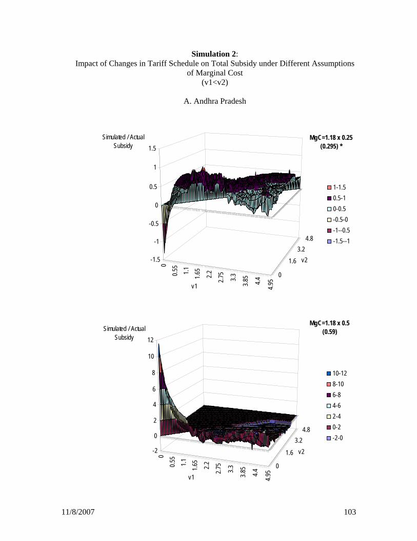
11/8/2007 103
Simulation 2: Impact of Changes in Tariff Schedule on Total Subsidy under Different Assumptions
of Marginal Cost (v1<v2)
A. Andhra Pradesh
00.5
51.1 1.6
5
2.2 2.75
3.3
3.85
4.4
4.95
0
1.6
3.24.8
-1.5
-1
-0.5
0
0.5
1
1.5Simulated / Actual
Subsidy
v1
v2
1-1.50.5-10-0.5-0.5-0-1--0.5-1.5--1
MgC=1.18 x 0.25(0.295) *
00.5
51.1 1.6
5
2.2 2.75
3.3 3.85
4.4 4.95
0
1.6
3.24.8
-2
0
2
4
6
8
10
12Simulated / Actual
Subsidy
v1
v2
10-128-106-84-62-40-2-2-0
MgC=1.18 x 0.5(0.59)
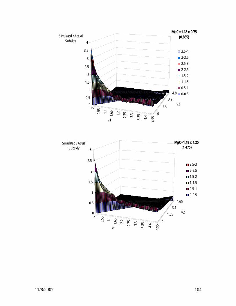
11/8/2007 104
00.5
51.1 1.6
5
2.2 2.75
3.3 3.85
4.4 4.95
0
1.6
3.24.8
0
0.5
1
1.5
2
2.5
3
3.5
4Simulated / Actual
Subsidy
v1
v2
3.5-43-3.52.5-32-2.51.5-21-1.50.5-10-0.5
MgC=1.18 x 0.75(0.885)
00.5
5
1.11.6
5
2.2 2.75
3.3 3.85
4.4 4.95
0
1.55
3.14.65
0
0.5
1
1.5
2
2.5
3Simulated / Actual
Subsidy
v1
v2
2.5-32-2.51.5-21-1.50.5-10-0.5
MgC=1.18 x 1.25(1.475)
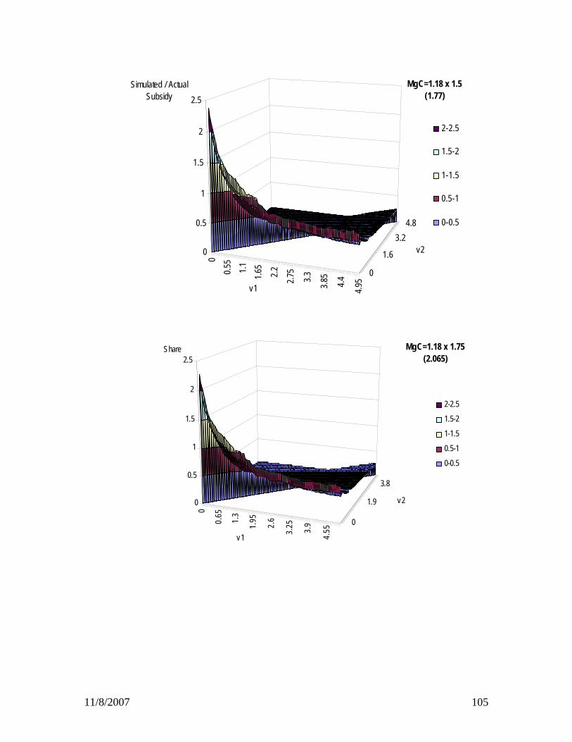
11/8/2007 105
0
0.65 1.3
1.95 2.6
3.25 3.9
4.55
0
1.9
3.8
0
0.5
1
1.5
2
2.5Share
v1
v2
2-2.5
1.5-2
1-1.5
0.5-1
0-0.5
MgC=1.18 x 1.75(2.065)
00.5
51.1 1.6
5
2.2 2.75
3.3 3.85
4.4 4.95
0
1.6
3.24.8
0
0.5
1
1.5
2
2.5Simulated / Actual
Subsidy
v1
v2
2-2.5
1.5-2
1-1.5
0.5-1
0-0.5
MgC=1.18 x 1.5(1.77)

11/8/2007 106
B. Punjab
00.5
51.1 1.6
52.2 2.7
5
3.3 3.85
4.4
4.95
0
1.6
3.24.8
-3-2.5
-2-1.5
-1-0.5
00.5
11.5
2Simulated / Actual
subsidy
v1
v2
1.5-21-1.50.5-10-0.5-0.5-0-1--0.5-1.5--1-2--1.5-2.5--2-3--2.5
MgC=1.89 x 0.25(0.4725) *
00.5
51.1 1.6
5
2.2 2.75
3.3 3.85
4.4 4.95
0
1.55
3.14.65
-1
0
1
2
3
4
5
6
7
8Simulated / Actual
Subsidy
v1
v2
7-86-75-64-53-42-31-20-1-1-0
MgC=1.89 x 0.5(0.945)

11/8/2007 107
00.5
51.1 1.6
5
2.2 2.75
3.3 3.85
4.4 4.95
0
1.55
3.14.65
0
0.5
1
1.5
2
2.5
3Simulated / Actual
subsidy
v1
v2
2.5-32-2.51.5-21-1.50.5-10-0.5
MgC=1.89 x 1.25(2.3625)
00.5
51.1 1.6
5
2.2 2.75
3.3 3.85
4.4 4.95
0
1.55
3.14.65
-0.5
0
0.5
1
1.5
2
2.5
3
3.5
4Simulated / Actual
Subsidy
v1
v2
3.5-4
3-3.5
2.5-3
2-2.5
1.5-2
1-1.5
MgC=1.89 x 0.75(1.4175)

11/8/2007 108
00.5
51.1 1.6
5
2.2 2.75
3.3
3.85
4.4
4.95
0
1.6
3.24.8
0
0.5
1
1.5
2
2.5
3Simulated / Actual
Subsidy
v1
v2
2.5-32-2.51.5-21-1.50.5-10-0.5
MgC=1.89 x 1.5(2.835)
0
0.55
1.1
1.65
2.2
2.75
3.3
3.85
4.4
4.95
0.5
2
3.50
0.10.20.30.40.50.60.70.8
0.91
Simulated / Actual subsidy
v1
v2
0.9-10.8-0.90.7-0.80.6-0.70.5-0.60.4-0.50.3-0.40.2-0.30.1-0.20-0.1
MgC=1.89 x 1.75(3.3075)

11/8/2007 109
Simulation 2: Impact of Changes in Tariff Schedule on Share of Smallholders in Total Subsidy,
under Different Assumptions of Marginal Cost (v1<v2)
A. Andhra Pradesh
0.5
1.2
1.9
2.6
3.3 4
4.7
0.55
2.6
4.65
00.1
0.20.3
0.4
0.5
0.6
0.7
0.8Share
v 1
v 2
0.7-0.8
0.6-0.7
0.5-0.6
0.4-0.5
0.3-0.4
0.2-0.3
0.1-0.2
0-0.1
v1=2.5; v2=3.5Share=25.4%
MgC=1.18 x 0.25(0.295) *
0
0.8
1.6
2.4
3.2 4
4.8
0
2.25
4.5
0
0.5
1
1.5
2
2.5
3Share
v 1
v 2
2.5-3
2-2.5
1.5-2
1-1.5
0.5-1
0-0.5
v1=2.5; v2=3.5Share=135.6%
MgC=1.18 x 0.75(0.885)
0
0.8
1.6
2.4
3.2 4
4.8
0
2.25
4.5
0
0.2
0.4
0.6
0.8
1
1.2
1.4Share
v 1
v 2
1.2-1.4
1-1.2
0.8-1
0.6-0.8
0.4-0.6
0.2-0.4
0-0.2
v1=2.5; v2=3.5Share=94.8%
MgC=1.18 x 1.25(1.475)
0
0.8
1.6
2.4
3.2 4
4.8
0
2.25
4.5
0
0.2
0.4
0.6
0.8
1
1.2Share
v 1
v 2
1-1.2
0.8-1
0.6-0.8
0.4-0.6
0.2-0.4
0-0.2
v1=2.5; v2=3.5Share=87.1%
MgC=1.18 x 1.75(2.065)

11/8/2007 110
B. Punjab
0.5
1.2
1.9
2.6
3.3 4
4.7
0.55
2.55
4.55
0
0.10.2
0.3
0.4
0.5
0.6
0.7
0.8Share
v 1
v 2
0.7-0.8
0.6-0.7
0.5-0.6
0.4-0.5
0.3-0.4
0.2-0.3
0.1-0.2
0-0.1v1=1.5; v2=2.5Share=17.5%
MgC=1.89 x 0.25(0.475) *
0
0.8
1.6
2.4
3.2 4
4.8
0
2.25
4.5
0
0.2
0.4
0.6
0.8
1Share
v 1
v 2
0.8-1
0.6-0.8
0.4-0.6
0.2-0.4
0-0.2
v1=1.5; v2=2.5Share=25.5%
MgC=1.89 x 0.75(1.4175)
0
0.8
1.6
2.4
3.2 4
4.8
0
2.25
4.5
0
0.2
0.4
0.6
0.8
1Share
v 1
v 2
0.8-1
0.6-0.8
0.4-0.6
0.2-0.4
0-0.2
MgC=1.89 x 1.25(2.3625)
0
0.75 1.5
2.25 3
3.75 4.5 0.5
2.6
4.7
00.10.20.30.40.50.60.70.8
0.9Share
v 1
v 2
0.8-0.90.7-0.80.6-0.70.5-0.60.4-0.50.3-0.40.2-0.30.1-0.20-0.1
v1=1.5; v2=2.5Share=23.9%
MgC=1.89 x 1.75(3.3075)

11/8/2007 111
Simulation 3 Ratio simulated / actual loss of electricity firm
A. Andhra Pradesh
0
0.9
1.8
2.7
3.6
4.5 0
2.5
5
0
0.5
1
1.5
2
2.5
3sim/actual loss
v 1
v 2
25% increase in FSubs first segment=57%
2.5-3
2-2.5
1.5-2
1-1.5
0.5-1
0-0.5
0
0.9
1.8
2.7
3.6
4.5
0
2.4
4.8
0
0.5
1
1.5
2
2.5sim/actual loss
v 1
v 2
50% increase in FSubs first segment=49%
2-2.5
1.5-2
1-1.5
0.5-1
0-0.5
0
0.9
1.8
2.7
3.6
4.5
0
2.4
4.8
-0.5
0
0.5
1
1.5
2
2.5sim/actual loss
v 1
v 2
75% increase in FSubs first segment=40%
2-2.5
1.5-2
1-1.5
0.5-1
0-0.5
-0.5-0
0
0.9
1.8
2.7
3.6
4.5
0
2.4
4.8
-0.5
0
0.5
1
1.5
2
2.5sim/actual loss
v 1
v 2
100% increase in FSubs first segment=32%
2-2.5
1.5-2
1-1.5
0.5-1
0-0.5
-0.5-0
0
0.9
1.8
2.7
3.6
4.5 0
2.5
5
-0.5
0
0.5
1
1.5
2
2.5sim/actual loss
v 1
v 2
125% increase in FSubs first segment=23%
2-2.5
1.5-2
1-1.5
0.5-1
0-0.5
-0.5-0
0
0.9
1.8
2.7
3.6
4.5 0
2.5
5
-0.5
0
0.5
1
1.5
2
2.5sim/actual loss
v 1
v 2
150% increase in FSubs first segment=15%
2-2.5
1.5-2
1-1.5
0.5-1
0-0.5
-0.5-0

11/8/2007 112
B. Punjab
0
0.8
1.6
2.4
3.2 4
4.8
0
2.2
4.4
0
0.5
1
1.5
2
2.5
3
3.5sim/actual loss
v 1
v 2
25% increase in FSubs first segment=30%
3-3.5
2.5-3
2-2.5
1.5-2
1-1.5
0.5-1
0-0.5
0
0.8
1.6
2.4
3.2 4
4.8
0
2.2
4.4
-0.5
0
0.5
1
1.5
2
2.5
3sim/actual loss
v 1
v 2
50% increase in FSubs first segment=16%
2.5-3
2-2.5
1.5-2
1-1.5
0.5-1
0-0.5
-0.5-0
0 1 2 3 4 5
0
2.7-0.5
00.5
1
1.5
2
2.5
3sim/actual loss
v 1
v 2
75% increase in FSubs first segment=2%
2.5-3
2-2.5
1.5-2
1-1.5
0.5-1
0-0.5
-0.5-0
0 1 2 3 4 5
0
2.7-0.5
0
0.5
1
1.5
2
2.5
3sim/actual loss
v 1
v 2
100% increase in FSubs first segment= -11%
2.5-3
2-2.5
1.5-2
1-1.5
0.5-1
0-0.5
-0.5-0
0
0.9
1.8
2.7
3.6
4.5
0
2.5
5
-0.5
0
0.5
1
1.5
2
2.5
3sim/actual loss
v 1
v 2
125% increase in FSubs first segment= -25%
2.5-3
2-2.5
1.5-2
1-1.5
0.5-1
0-0.5
-0.5-0
0
0.9
1.8
2.7
3.6
4.5
0
2.4
4.8
-0.5
0
0.5
1
1.5
2
2.5sim/actual loss
v 1
v 2
150% increase in FSubs first segment= -39%
2-2.5
1.5-2
1-1.5
0.5-1
0-0.5
-0.5-0