plasma sail propulsion based on the plasma...
TRANSCRIPT

The 30th International Electric Propulsion Conference, Florence, Italy
September 17-20, 2007
1
Plasma Sail Propulsion Based on the Plasma Magnet
IEPC-2007-15
Presented at the 30th International Electric Propulsion Conference, Florence, Italy September 17-20, 2007
John Slough*
University of Washington, Seattle, WA, 98195, USA
Abstract: Propulsion based on the plasma magnet taps the ambient energy of the solar wind via the coupling to a large-scale (30 km) dipolar magnetic field generated by two polyphase antennae that drive currents in the plasma to create, inflate and maintain the magnetic structure. In scaled a laboratory experiment, all aspects of the plasma magnet as a propulsion system were explored and validated. A solar wind source (SWS) of the appropriate flow velocity and power was deflected by a plasma magnet whose antennae were attached to a ballistic pendulum. A large displacement attributable only to the deflection of the SWS by the plasma current generated dipole magnetic fields was observed. The inferred thrust from deflection of the SWS was 2N during the time of operation providing an equivalent “jet” power of 1 MW.
Nomenclature BRMF = magnitude of rotating magnetic field B = magnitude of steady axial magnetic field BMP = magnitude of magnetospheric field at the magnetopause β = ratio of plasma to magnetic field energy density i.e. nkT/(B2/2μ0) Isp = Specific Impulse δ = classical skin depth in a conductor D⊥ = particle diffusion coefficient Eθ = azimuthal component of the induced electric field EB = energy stored in magnetic field Iθ = total driven azimuthal current jθ = azimuthal current density ne = plasma electron density N = particle inventory of plasma magnetosphere νei = electron-ion collision frequency r = radial distance in cylindrical coordinates MHD = Magneto-Hydrodynamics PRMF = power delivered into plasma by RMF antenna Psw = jet power to plasma magnetosphere from deflection of solar wind RMF = Rotating Magnetic Field R0 = radius of the Rotating Magnetic Field Antenna RMP = distance from the spacecraft antenna and the magnetopause along the spacecraft-sun line RLMP = stand-off distance to magnetopause in laboratory solar wind experiment. ρsw = ion gyroradius of a solar wind ion in the plasma magnetosphere τN = particle confinement time
* Res. Assoc. Prof., Department of Aeronautics and Astronautics, [email protected]

The 30th International Electric Propulsion Conference, Florence, Italy
September 17-20, 2007
2
SWS = Solar Wind Source Te = electron temperature (electron volts) ω = rotation frequency of the rotating magnetic field ωce = eBRMF/me electron cyclotron frequency in the rotating magnetic field BRMF ωci = eBRMF/mi the ion cyclotron frequency
I. Introduction LASMA sail propulsion based on the plasma magnet is a unique system that taps the ambient energy of the
solar wind with minimal energy and mass requirements. The coupling to the solar wind is made through the generation of a large-scale (~> 30 km) dipolar magnetic field. Unlike the original magnetic sail concept, the coil currents are conducted in a plasma rather than a superconducting coil. In this way the mass of the sail is reduced by orders of magnitude for the same thrust power. The plasma magnet consists of a pair of polyphase coils that produce a rotating magnetic field (RMF) that drives the necessary currents in the plasma to inflate and maintain the large-scale magnetic structure. The plasma magnet is deployed by the Lorentz self-force on the plasma currents, expanding outward in a disk-like shape until the expansion is halted by the solar wind pressure. It is virtually propellantless as the intercepted solar wind replenishes the small amount of plasma required to carry the magnet currents. Unlike a solid magnet or sail, the plasma magnet expands with falling solar wind pressure to provide a constant force.
In phase I a small prototype plasma magnet was built and tested. The phase I experiments demonstrated the ability to drive sufficient current in the plasma magnet to have the resultant dipole field push out well beyond the 10 km scale required for significant interaction with the solar wind. The RMF coils generated over 10 kA of plasma currents with a radial expansion pressure sufficient to expand the dipole field to well over the 30 km scale that would supply as much as 5 MW of thrust power. In addition it was demonstrated that a large force imparted on the plasma magnet was reacted back on the RMF antennas with no plasma detachment. The most significant issues left to be tested in validating the plasma sail concept based on the plasma magnet were three-fold. (1) It must be shown that the plasma magnet can achieve an equilibrium configuration in the presence of a larger scale solar wind, and (2) that the expected thrust is actually imparted to the antenna structure. (3) It must be demonstrated that the system scales as predicted by code and theory based on the experimental results at small scale. The expected near linear dependence of dipole field with radius under compression from the solar wind, allows for a scaled experiment that should be very close to producing the results one should obtain in space. With the construction of the proper solar wind source, all of the key dimensionless parameters are unchanged by scaling to a smaller experiment. The only parameter that will not scale is the collisionality of the plasma. As was seen in the phase I demonstration, the current carrying plasma is essentially collisionless even near the source where the plasma density is highest, so this should not be a major concern.
The two key experimental tasks for the phase II study were thus: (1) achieve an equilibrium configuration with supersonic flowing plasma (solar wind), and measure the thrust delivered to the plasma magnet structure. Both of these tasks were successfully completed. To create a more space-like environment free of interference from skin currents in metal conductors, a new experimental device was constructed that was comprised of a large dielectric chamber. A new control and data acquisition system was designed and implemented that was capable of obtaining much more detailed equilibrium measurements as well as the thrust measurement. In addition, a multi-megawatt surrogate solar wind source was designed and constructed.
Several key experimental results were obtained in the initial tests. A scaled version of the RMF antenna geometry to be used in space was constructed and tested. A successful demonstration of the desired plasma current generation and expansion was achieved. Here the primary plasma currents were initially produced within the antenna, and were then found to expand radially outward achieving an equilibrium outside the antenna structures as it must be in space. This was the first time where the primary plasma currents have been generated and sustained using the outer field of the rotating dipole field.
A fully 3D numerical model was developed, and analytic analysis sufficient to understand the experimental observations and make scaling predictions was formulated. The 3D MHD model of the RMF generated plasma has was performed. Initial results indicate the generation of the steady dipole magnetic field observed in the experiments with the governing parameter during current ramp-up being the collisionless ion skin depth. The basic theoretical scaling of the antenna power with the space craft relevant parameters has also been undertaken indicating a very favorable scaling with antenna size. Point designs for antenna radii of 100 m and 1 km were preformed.
P

The 30th International Electric Propulsion Conference, Florence, Italy
September 17-20, 2007
3
The hallmark of the phase II effort was the successful completion of the laboratory scaled experiments with the intensified solar wind source. All aspects of the plasma magnet performance as a propulsion system were validated. A solar wind source (SWS) of the appropriate flow velocity and power was operated and characterized. The antenna plasma magnet RMF structure was built and installed in the large dielectric chamber as a counterweighted ballistic pendulum. A fiber optic position sensor was used to detect thrust imparted to the antenna from deflection of the SWS hydrogen plasma. A large displacement attributable only to the deflection of the SWS by the plasma current generated dipole magnetic fields was observed. The momentum transfer was thus successfully demonstrated.
The plasma magnet was observed to contract and expand in response to changes in the SWS plasma flow demonstrating that a dynamic equilibrium in a flowing plasma can be maintained. The interception of the initial SWS plasma was used to bootstrap the initial inflation of the plasma magnet making for a propellantless propulsion device. A much expanded plasma magnet persisted long after the SWS pulse indicating an enhanced plasma confinement characteristic observed in plasmoids generated and sustained by RMF. The average thrust during the 200 μs pulse length was 2 N. With a characteristic SWS flow speed of 50 km/s, the thrust power observed was 1.0 MW. Higher thrust power was limited by both the flow speed of the SWS that could be achieved and arcing limitations due to an antenna insulation failure. Additional enhancement of the deflection radius is expected as the system becomes more MHD-like (a small ion Larmor radius compared to the plasma magnet radius). The plasma magnet/SWS system tested was still in the kinetic regime where ion deflection was incomplete.
With the successful demonstration of thrust power at the MW level, a final large tank test or possibly even a space demonstration with a microsat could be undertaken. These experiments would provide the final confirmation of the scaling for a deep space mission.
II. Background It is very difficult for any propellant based rocket
to satisfy the thrust and high Isp requirements for outer planetary, manned planetary, or interstellar missions of the future. The power requirements are very much larger than can be supported by present, planned, or imagined solar electric systems (a few hundred kW at most). Without power system in the megawatt class, access to deep space becomes very limited. There is certainly significant promise for any device that can generate megawatts of thrust power with minimal, kilowatt level, on-board power, and minimal fuel requirements. The device that will be described here, the plasma magnet, has such potential.
In order to achieve propulsion power greater than that which can be supplied from onboard sources, whether chemical or nuclear, the spacecraft must be supplied by an external source. What is being proposed here is to tap the solar plasma energy i.e. the solar wind. The mechanism for the transfer of momentum from the outwardly streaming solar plasma is through the capture or deflection of the solar wind by the interaction of the plasma with a large scale magnetic field. This magnetic field is anchored to the spacecraft through the electromagnetic force between the field current and the spacecraft antenna fields. The magnetospheric currents are generated and sustained by a rotating magnetic field created by the antenna structure, and it is ultimately the antenna to which the solar wind induced force is reacted. This plasma current based magnetospheric system is herein referred to as the plasma magnet (see Fig. 1). The fact that the solar wind produces a net force on a magnetosphere can be observed in numerous astrophysical phenomena1. The magnitude of this force has been quantified by numerical calculation with both MHD2 and kinetic models3 at size scales relevant to the concept presented here. The physical principles involved in the plasma magnet current generation are well understood4, and have been demonstrated in laboratory experiments 5,6. There are several other possible applications for the plasma magnet, but the singularly most important aspect of the plasma magnet is the possibility of achieving very high (multi-Megawatt) thrust powers.
SolarWind Polyphase antenna hoops
Steady dipole fieldfrom plasma currents
Figure 1. Plasma Magnetic Sail based on rotating magnetic field generated plasma currents. Two polyphase magnetic coils (stator) are used to drive steady ring currents in the local plasma (rotor) creating an expanding magnetized bubble. Expansion is halted by solar wind pressure is in balance with the magnetic pressure from the driven currents (R ≥ 10 km). The antennas (radius ~ 0.1 km) are shown expanded for clarity

The 30th International Electric Propulsion Conference, Florence, Italy
September 17-20, 2007
4
The initial proposals to harness the energy of the solar wind were by reflection off a magnetic wall or MagSail7. Here the basic concept was to deploy a huge superconducting magnet with a radius of ~ 30 km. A system of this size (~ a few metric tons) would only attain accelerations of the order of 0.01 m/s2. The current density requirements for the superconducting ring are well beyond that of current high temperature superconductors, and, as with all fixed area sails, there is the problem of the thrust only being significant near the sun.
There have been other schemes for obtaining propulsive power from the solar wind. Within the generic heading of plasma sails, the Mini-Magnetospheric Plasma Propulsion (M2P2) was the first to address the possibility of harnessing the solar wind for propulsion via an artificial magnetosphere8. It is similar to the plasma magnet in that both make use of the ambient energy of the solar wind by coupling to the solar wind through a large-scale (~ > 10 km) magnetic bubble or mini-magnetosphere. Plasma sails utilize electromagnetic processes (as opposed to mechanical structures) to produce the obstacle or sail. Thus the technical and material problems that challenge traditional solar sails are removed from the problem. In the initial M2P2 embodiment of the plasma sail concept, the magnetosphere was to be inflated by the injection of plasma on to the magnetic field of a small (< 1 m) dipole coil tethered to the spacecraft. The main difficulty with this approach to capturing the solar wind is the inflation of the relatively minuscule dipole field. The conditions required for inflation can be readily derived9, but it can be seen that the magnetosphere must be inflated by plasma pressure, and the amount of expansion is directly proportional to the source plasma “beta” – the ratio of plasma energy to the local magnetic field energy, ie. β = nkT/(B2/2μ0). This makes for a significant challenge in that a local source of high β plasma is difficult to sustain during initial inflation at magnetic fields strengths large enough to generate a multi-kilometer size M2P2, much like a balloon is most difficult to inflate when small and the internal tension is high. The flux available to expand and interact with the solar wind is also limited to that which can be generated in the small dipole coil. Although this flux can be expanded by a high β plasma, it can not be directly increased. It must be energized by the interaction with the solar wind, which cannot occur until the mini-magnetosphere is tens of kilometers in size. The thrust that can be developed by an M2P2 is thus ultimately limited by the magnetic flux of the on-board magnet. This is not the case for the plasma magnet. Like the MagSail the plasma magnet creates and sustains a large scale current, and thus large magnetic flux but without the mass penalty.
The ultimate spacecraft speed powered by the plasma magnet is that of the solar wind (350 to 800 km/s) which is orders of magnitude higher than the Isp limitations of existing plasma thrusters. As opposed to the solar sails and the MagSail, the dynamic nature of the plasma magnet assures a constant thrust in that it will expand as the solar wind dynamic pressure decreases with distance from the sun. As such, it will provide an almost constant acceleration to the spacecraft as it moves out into the solar system. The solar wind experiences essentially no deceleration until the termination shock at approximately 80 +/- 10 AU. The plasma magnet could thus be used for missions all the way to the Kuiper belt. In the initial embodiment for the plasma magnet, only solar electric systems are considered. This effectively limits the acceleration period to ~ 3 months (and the spacecraft speeds to 50 –80 km/s). If larger electric systems become available that could provide a few tens of kilowatts of power, or if powered by either radioactive
Figure 2. Illustration of the plasma magnet inflation. The rotating dipole field (blue field lines) is seen in the first frame as the dominant field at small scale. As more plasma is entrained, the steady dipole field (red field lines) arises from the synchronous azimuthal flow of electrons (red dots). The rotating field is convected outward with the expanding current ring (second frame). The expansion continues with the dominant field now being the steady dipole field forming the magnetospheric object that ultimately comes into a dynamic balance with the solar wind pressure at radius of 20 km or more (50 to 200 times the initial plasma magnet size).

The 30th International Electric Propulsion Conference, Florence, Italy
September 17-20, 2007
5
isotopes or nuclear power, speeds of several hundred km/s are possible.
The rotating magnetic field (RMF) that maintains the large-scale dipole currents can have a very simple geometry e.g. a pair of wire hoops. The hoop antenna can be deployed through the self force arising from the magnetic field generated by the oscillating currents in the hoop. As will be seen, the rotating field is quite small compared to the steady field that is produced by the driven currents. The ratio of solar wind power to the power dissipated in the plasma magnet scale favorably with size, so that large, kilometer-scale hoops are thus envisioned. The current waveform for the polyphase antennas is that of a simple sinusoid which can be produced by a resonant tank circuit. Such a circuit operates at high efficiency so that virtually the only power required stems from the small ohmic losses in sustaining the magnetospheric plasma currents. Even though the plasma may be more resistive than the superconducting wires of the MagSail, the huge difference in cross sectional area that the plasma subtends (km2 vs. cm2) minimizes the additional power requirement.
The essential aspect of the plasma magnet is the ability to directly drive the currents needed for the large-scale magnetosphere itself. Since the plasma electrons are magnetized in both the steady dipole field generated by the rotating magnetic field, as well as the RMF, the plasma expansion effectively makes an ever-increasing plasma magnet, and ever increasing magnetic flux. This is subject of course to having a sufficiently large rotating field to counter the electron drag from plasma resistance. The plasma expands under the self (hoop) force arising from the driven currents until halted by the solar wind pressure, which acts as a confining force as it does in planetary magnetospheres. As plasma diffuses outward in the steady dipole field, it is still driven by the rotating field and will still continue to generate a confining steady dipole field. In this way the plasma diffusion is countered by flux generation. In laboratory experiments the plasma was confined for orders of magnitude longer than that predicted by classical Spitzer resistivity6. It is quite possible that a plasma magnetic sail, driven and sustained by a rotating magnetic field, would be nearly propellantless, particularly if it traps the solar wind particles it intercepts.
The key elements for the validation of this concept depend on (1) a favorable scaling based on the fundamental physical principles of RMF current drive; (2) the experimental demonstration of the generation and sustainment of a plasma magnet in a space-like environment, and. (3) the demonstration of thrust from the interaction of a flowing plasma and a plasma magnet. These three elements were successful demonstrated in experiments conducted on the plasma magnet. Results from the first of these elements will be covered in the next section. The second element has been carried out in the first phase of experiments, and will be described in section IV. The final element has been recently completed in a larger dielectric chamber, and a description of these experiments will follow in section V.
III. Analysis and Scaling of the Plasma Magnet An analysis of the scaling of the plasma magnet begins with a examination of the mechanisms involved in the
generation of the plasma currents by the rotating magnet field (RMF). From this analysis the basic scaling of the plasma sail thrust power with the RMF power is derived. It is possible with these results to obtain a point design for the plasma magnet based plasma sail in terms of the key parameters. A point design based on the experimental results obtained so far will be given.
A. Current production employing rotating magnetic fields (RMF) The plasma magnet generates the large scale currents needed for a large-scale magnetosphere by the entrainment
of the plasma electrons in a rotating field created by two pair of loop antennae (see Fig. 1). With the loops separated by 90 degrees in azimuth, and with their respective currents separated in phase by 90 degrees, a steady magnetic field rotating in the equatorial plane is produced. In analogy to the induction motor, this is the same as the field that is produced in a two pole stator winding. Normally a “squirrel cage” rotor would be inserted inside these coils and the currents induced in the rotor by the rotating field, together with the stator magnetic field, produce the torque that causes the rotor to come into synchronous rotation with the field. Consider the case now where the metal rotor is replaced with a plasma rotor. With nearly zero mass, the electrons quickly come into co-rotation with the RMF. The rigid rotation of the electrons is retarded slightly by collisions with the much more massive background ions which, due to their large inertia are unable to respond to the rapidly rotating field and remain relatively motionless. In this manner a large azimuthal (θ) current is driven in the plasma. The magnetic field generated by the rotor currents couple it inextricably with the stator fields. Like any AC motor, a force applied to the rotor is reacted back on to the stator through these fields without any physical contact between the two. The same momentum transfer occurs with the plasma rotor as well. The eventual “load” on the plasma rotor will be the drag of the solar wind plasma, with the force of the solar wind reacted back onto the RMF antenna loops (the stator) attached to the spacecraft. Currents
The 30th International Electric Propulsion Conference, Florence, Italy
September 17-20, 2007
6
driven by the RMF find an analogous representation in the ring currents formed when the magnetosphere is rapidly compressed by the solar wind. The process of course is reversed for the plasma magnet where the driven ring current acts to expand the magnetic bubble pushing off the solar wind.
For the plasma magnet to have a high efficiency, just as it is for the AC motor, there should be as little internal resistance as possible, i.e. the “no load” slip should be small. For the plasma this is the equivalent of satisfying two conditions: For there to be as large a current as possible, the ions should be unable to respond to the rotating field due to their inertia. This condition is equivalent to the ions being unmagnetized, or
ω > ωci (1a)
where ωci is the ion cyclotron frequency in the RMF. The slip due to the plasma resistivity is completely analogous to the rotor slip in a motor due to resistive losses in the rotor. For the plasma rotor, the condition for a small slip is stated in terms of the plasma collisionality:
νei << ωce (1b)
where ωce is the electron cyclotron frequency in the RMF. This inequality is equivalent to stating that the electrons are well magnetized to the RMF. A starting point for understanding the current drive process is the generalized Ohm’s Law, where it will be assumed for the moment that the ions form a fixed uniform background and the u×B term can be ignored. The azimuthal (equatorial) current is determined by the θ component:
(2)
where B has oscillating components in the θ and r directions due to the RMF at a frequency ω, and a steady axial field Bz produced mainly by the RMF. With a rotating field, the Hall term acting in the θ direction is comprised of a pondermotive component - the <jzBr> term. Since the axial screening current jz and Br vary similarly in time at the frequency ω, the pondermotive force in the θ direction has both a steady part and an oscillatory part at a frequency of 2ω. From the steady <jzBr> force, the electron fluid will attain that steady value of azimuthal velocity, ueθ that corresponds to the balancing of the steady accelerating torque induced by Eθ, with the retarding torque due to the collisions of the electrons with the ions. In this way a steady azimuthal current density, jθ is generated. For synchronous electrons, the azimuthal current density is given by:
jθ = -neωr (3)
where n(r) is the plasma density and r is the distance from the polar axis. This “rigid rotor” current density profile is characteristic of a low-slip RMF driven plasma. Operating the RMF antenna in this manner, very large (20 kA) currents have been generated in a plasma as small as 5 cm radius10. By having the azimuthal currents inside the RMF antenna, the expansion force of the current ring can be countered by an axial magnetic field produced by a coil surrounding the plasma just inside the RMF antenna. In this way a steady equilibrium can be established.
An additional requirement on the RMF is that it remains penetrated in the plasma. The solution of Ohm’s law, neglecting the Hall term, is characterized by the RMF penetrating a distance δ = (2η/ωμo)1/2, which is the resistive skin depth for an RF field into a conductor. However, the regime of interest here is a near collisionless plasma where νei << ωce. From the viewpoint in the frame of the rotating field, the co-rotating electrons experience a nearly constant transverse field. The effective field penetration depth can be many times the resistive skin depth as the apparent frequency of the RMF in the frame of the electrons is near zero. It should be recalled that RMF coils produce a dipole field that rotates in space with the dipole oriented with its axis in the equatorial plane of the steady dipole field. The discussion above has focused primarily on the current that can be generated by the synchronous rotation of the electrons on the inner dipole field region of the RMF. Until the experiments reported here, this is what had been extensively studied in the laboratory. To generate a large scale dipole magnet, one wants to turn the normal RMF current drive geometry inside out, with the plasma located in the region external to the RMF antennas as depicted in Fig. 2. From this figure, it can be seen that the outer field of the RMF dipole can be employed to drive
cer z z r z
ei
1E u B j j B j jneθ θ θ
⎡ ⎤⎛ ⎞ω+ = η + = η +⎢ ⎥⎜ ⎟ν⎝ ⎠⎣ ⎦

The 30th International Electric Propulsion Conference, Florence, Italy
September 17-20, 2007
7
β ~ 0
β ~ 10
(dipole enlarged 10x)β ~ 0
β ~ 10
(dipole enlarged 10x)
Figure 3. High β dipole equilibrium. Flux lines in R-Z plane for analytic equilibrium solution for a point dipole configuration at high β.
azimuthal (equatorial) currents outside the dipole as long as there is plasma in this region, and indeed that is what was observed in the experiments.
With no external field to oppose the Lorentz self-force acting on the plasma azimuthal currents, the current ring expands. The only confining force is that of the curvature forces from the steady dipole field created by the RMF driven currents. This force is sufficient to keep the plasma in a high β equilibrium as it expands (the driven current is equivalent to a plasma diamagnetic current in equilibrium). Since the gyroradius of a solar wind ion will be much larger than the initially sub-kilometer size expanding dipole, little distortion of the dipole from the solar wind is expected until the plasma magnet has expanded large enough to interact with the solar wind. In addition to expanding the dipole, the driven currents will change the equilibrium field shape significantly from the vacuum field. Realistic equilibria for the magnetic dipole with large diamagnetic currents have been found and analyzed11. It was found that plasma pressure profiles P(ψ) that fall off at least as slow as the adiabatic rate (~ ψ20/3), where ψ is the flux surface coordinate, were stable to both interchange and ballooning instabilities12. This is significant in that a well-confined plasma is important for maintaining a low plasma resistance as an anomalous plasma resistivity increases the amount of power that must be delivered to drive the same current. The modification to the dipole flux function ψ (= sin(θ)2/r in vacuum) at high β can be expressed as:
, (4)
where the zero subscript refers to a reference surface near the RMF antenna. As the current is increased, the flux function is considerably modified from the vacuum case as can be seen in Figure 3. The flux surfaces become more disk-like as the plasma expands. This is primarily due to the lower magnetic field of the dipole near the equatorial plane. As the plasma current (pressure) is raised, the dipole field is distorted into a shape that enhances the curvature force at the point of lowest field pressure (i.e. the equatorial region). In the limit of β → ∞ (the plasma pressure equal to the external field pressure), the dipole field B(r) ~ B0R0
2/r2. With β>>1, the dipole field drop-off will at best be no slower than 1/r2. This can be seen from flux conservation. It is clear that the high β plasma will expand the flux over a much larger region (with equatorial area A). The initial dipole flux ϕ0 = B0A0 must equal BA at any point later. One has then that B ∝ 1/A ~ 1/r2. By directly driving the electrons in the outer magnetosphere, the plasma magnet grows with the expansion of the current ring.
The steady dipole field can thus have a much slower than 1/r2 fall-off. An increasing magnetic field could be generated with a sufficiently large RMF as nothing prohibits the expanding plasma from producing essentially as much current as Ohm’s Law and the power supply will allow (see Eq. 3). The plasma is both created and ohmically heated by these RMF driven currents. Ohmic electron heating should only help to lower the plasma resistance making it even easier to drive a larger magnetosphere. The RMF current is driven in an inherently steady manner, which allows for the continued expansion and sustainment of the configuration.
With the electrons magnetized to the RMF, the RMF is convected along with the dipole field as it expands, but the RMF will fall off as 1/r2 as indicated in Eq. (4) since there is no more rotating flux than that produced by the antennas. It was found in previous numerical calculations that the solar wind compresses the steady magnetic dipole field inside a magnetosphere producing approximately a 1/r fall-off. The solar wind compresses both the RMF as well as the steady magnetic dipole field produced by the RMF, but this enhancement is not required here for the RMF to produce a 1/r fall-off in the steady dipole field. It can provide the necessary currents at sufficiently large radius to provide the 1/r fall-off without any enhancement from solar wind compression. This extra leverage assures that the magnetosphere produced by the plasma magnet will be of sufficient size regardless of the actual solar wind enhancement. The solar wind should only make it easier. To see how the 1/r dependence can be achieved by the plasma magnet alone, one determines the distribution of the RMF driven current density jθ required to produce a magnetic field dependence, B(r) ~ B0R0/r. From Ampere’s law one has then:
2/1000 ,
r)sin(R −
αα β=α
θψ=ψ

The 30th International Electric Propulsion Conference, Florence, Italy
September 17-20, 2007
8
. (5)
Equating this expression with that for RMF current drive [see Eq. (3)], it is observed that the plasma density can fall off as rapidly as n(r) ~ 1/r3, and still maintain the 1/r scaling for the dipole field. For a constant source production rate and no radial confinement (much like the solar wind), one has n ~1/r2. Any plasma confinement, as well as any plasma introduced by the solar wind should provide a steeper density fall-off. Driving more current than required for a 1/r is not a desirable condition in any case, as the RMF power required to drive the larger currents at large radius increases dramatically for a density drop-off less than 1/r3 (i.e. a field drop-off that is less than 1/r). As the field expands then, the frequency of the RMF can be decreased proportionately to help maintain the jθ scaling desired [see Eq. (3)]. Reducing the RMF frequency would be required in any case for a very large plasma magnet, to keep the synchronous electrons from becoming relativistic. Without solar wind compression the electron cyclotron frequency will fall off with the RMF field or, ωce ~ BRMF ~ 1/r2. The electron-ion collision frequency falls even faster, νei ~ ne ~ 1/r3, so that even with a decreasing frequency Eq. (1a) remains satisfied. This dependence assures that if the RMF can drive the plasma near the antenna coils, it can drive a magnet of any radius as long as the density-rotation frequency product neω falls as ~ 1/r3 or steeper. In fact, a slower fall-off can most likely be sustained, since any heating of the magnetospheric plasma from the solar wind (and a large degree of heating is expected with compression) νei will decrease as T-3/2 as well.
The confinement of the plasma in the plasma magnet dipole field can be expressed as:
, (6)
where it has been assumed that the density decreases as 1/r3. With this assumption, the total plasma inventory N can be calculated with N ~ 4πR3n0 ln(r/R). For an RMF antenna with R0 = 100 m with sufficient current (i.e. a particle density n0 ~ 1016 m-3) to inflate to r = 40 km bubble, one has τN = 4.5x10⁷ s ~ 15 years! The total plasma mass for this bubble is mp·N = 1.8 mg for hydrogen. Clearly refueling should not be a major concern for any working gas including Xenon. The confinement of the plasma in the plasma magnet is a quantity that, most likely, will be determined empirically. In any case, once the expansion is complete, confining the plasma in a large scale plasma sail looks to be relatively undemanding. The simplest and most desirable method to achieve the desired density falloff is to simply reduce the particle flow from the source. If the confinement is good enough, or the entrainment of the solar wind sufficient, the source plasma fueling may be completely turned off. If too great a density build-up should occur, it would be suppressed by the nature of the current drive process itself. As the density increases, the driven current increases. This in turn increases the dipole magnetic field, and leads to a further expansion of the magnetosphere. The expansion drops the density, which reduces the current, and a new equilibrium is achieved. The expansion of the dipole is now only limited by the ohmic power needed to maintain the structure from resistive dissipation. To make a simple estimation of what this power would be, consider the case of an azimuthally uniform magnetic field where the 1/r dependence is found in all directions. This clearly represents the highest power loading, as this uniformly high field configuration demands the highest total current density (like a solar wind from all directions). The RMF power, PRMF, needed to sustain the plasma magnet in this configuration is given by:
(7)
where Eq. (5) was used for jθ and B0 represents the steady dipole field strength near the RMF coils. B0 in Eq. (7) can be restated in terms of the final expansion field and size based on the assumed 1/r field scaling:
(8)
Here BMP is the magnetic field strength that is required to deflect the solar wind (i.e. the magnetopause field strength) and RMP is the distance to the magnetopause along the Sun-magnetosphere line. For a solar wind density of 6x10⁶ m-3 and a speed of vsw = 450 km/s, the solar wind represents a dynamic pressure equal to 1 nPa. A magnetic
20
00
0 rRB
drdB1j
μ=
μ=θ
20
2N r
Rrln
32
drdnDr4
dvoln⎟⎠⎞
⎜⎝⎛
βημ
=π
⋅=τ
⊥⊥
∫
0202
0
R
R22
0
20
202
RMF
RB4
drr4RBdVoljP
M
0
μπη
≅
πμ
η≈⋅η= ∫ ∫θ
0
MPMP0 R
RBB =

The 30th International Electric Propulsion Conference, Florence, Italy
September 17-20, 2007
9
field BMP = 50 nT is sufficient to produce an equivalent magnetic pressure. One can ignore the solar magnetic pressure, as it is negligible compared to the supersonic plasma flow of the solar wind. From numerical calculations8, it was found that the radial cross-sectional distance of the magnetosphere is roughly the same as the standoff distance RMP. The thrust power from the solar wind intercepted by the magnetosphere is approximately:
. (9)
This expression can be restated in terms of PRMF using Equations (7) and (8) where it is assumed that the RMF power is half that found in Equation (7), since the solar wind is only in one direction. The result is:
, (10)
where Spitzer resistivity η ~ 1.2x10⁻³ Te-3/2 with Te ~ 15 eV was assumed. These values correspond to those that
were observed in the plasma magnet experiments. With the lower current and density requirements for the plasma magnet, a much higher Te should be achievable. For the purposes of the scaling here, the more conservative estimate of the plasma resistivity will be used. The tremendous leverage in power one obtains from the plasma magnet can be easily seen from the numerical coefficient in Eq. (10). With a 100 m scale antenna and a RMF power of 1 kW, a space based plasma magnet could produce a thrust power Psw ~ 700 MW. Considerably higher resistivity and drive inefficiencies can be tolerated before it would become disadvantageous to pursue this form of propulsion.
The conditions required for the product of B0R0 to achieve a magnetosphere with a magnetopause standoff distance, RMP of 10 km, can be determined from Eq. (8) above and is 5x10⁻⁴ T-m. For example, this could correspond to an initial field B0 = 0.5 G, generated at the antenna radius R0 = 10 m. An estimate of the total driven current required in any case can be found from Ampere’s Law assuming a disk-like dipole magnetosphere found in the equilibrium solutions at high β (see Fig. 3). The total current required in the plasma magnet to achieve the 1/r falloff would be:
. (11)
Even in the extreme case where all of the plasma currents are generated by the RMF, the total driven current is less than what has been achieved in the recent plasma magnet experiments. It is also noteworthy to realize how relatively little energy must be invested in the plasma and field to produce a plasma sail with a dimensions on the order of 10s of kilometers. The magnetic energy within the plasma sail is given roughly by:
(12)
where the slower falloff of B ~ B0R0/r has been assumed (maximum field energy). At a sail size of 30 km, and recalling that solar wind pressure corresponds to a field pressure, BMP ~ 50 nT, the total magnetic energy is 84 kJ. For perspective, a car battery stores 1 MJ.
B. Plasma magnet design based on experimental results and analytic scaling. For a point design, the scale of the antenna is chosen primarily on what makes sense for the space based
application more than a parameter optimization. The obvious first undertaking would be a science mission where rapid deployment into the outer solar system and beyond was essential, and the need for precise orbit maneuvering minimal. The system performance can be evaluated in terms of the key parameters of antenna mass, MA, the spacecraft available on-board power, PS and antenna radius RA. Once a final plasma sail size has been decided upon, most of the remaining parameters can be determined. Based on all of the numerical work that has been done to date, for a substantial interaction of the plasma sail with the solar wind, the stand-off distance of the magnetopause, RMP, ~ 30 km at the earth radius (1 AU) would be sufficient. At 1 AU the magnitude of the magnetic field BMP required to balance the solar wind pressure was determined to be 50 nT. The product of field and size is thus:
CBR = BMP·RMP = 1.5 mT-m = B0·R0 (13)
2MP
0
2MP
swMPswsw R2Bv~FvP π⋅μ
⋅=
RMF03
RMF0SW0
SW PR10x7PRv4
~P =ημ
[ ] kA9rlnRB2dsB1I 0
M
RR
0
00
0r/1 =
μ≈⋅
μ= ∫
3MP
2MP
0MP
20
20
0
R
R
22
0
20
20
R
R 0
2
B RB2
RRB2
drr4r2
RBdVol2
)r(B~EMP
0
MP
0μπ
=μπ
=π⋅μ
=⋅μ ∫∫

The 30th International Electric Propulsion Conference, Florence, Italy
September 17-20, 2007
10
where Eq. (8) was employed to make clear that this product is a constant all the way in to the region near RMF antenna.
From Eq. (9), the effective “jet power” delivered by the solar wind, PSW, can be stated in terms of this constant. With the previous value assumed for the solar wind speed (450 km/sec) one obtains:
6.3 MW (14)
where an additional constant, CD has been included. This is the drag coefficient for a plasma sail whose cross-sectional area is stated in terms of the stand-off area πRMP
2 as it was done in Eq. (9). It has recently been found through MHD calculations15 that CD ~5 for the case where the dipole axis is aligned along the sun-spacecraft line as anticipated for the RMF driven plasma sail.
One now needs to calculate the power requirements for sustaining the plasma magnet. From Eq. (10) it is clear that the plasma dissipative losses will be low for any size antenna, but losses in the antenna structures maintaining the RMF may not be. One needs to relate the local magnetic field B0 produced by the driven currents to the magnitude of the RMF field required to produce those currents. It can be shown from the basic condition for current drive that:
(15)
where δ = (2η/ωμo)1/2, the collisional skin depth. As the antenna increases in size, the magnitude of the required driving field should decrease. Experimentally it has been found that the frequency for optimum current drive is found to decrease with an increase in the RMF system size. As indicated by Eq. (3), for the given current profile (plasma magnet size) to remain the same as one increases RMF antenna size, the product of ω and RA should be held constant. Assuming one adjusts ω ~ 1/RA as the antenna is enlarged, Eq. (15) can be rewritten as:
. (16)
The proportionality constant, κ, incorporates the plasma resistivity, and was specified to fit the observed ratio of the steady dipole field to RMF field at the origin in current experiments. There could be an additional dependence of the resistivity with size, but it will be assumed constant as this is a parametric dependence that will no doubt require experimental determination as in virtually all plasma configurations.
The power dissipated in the antenna can now be estimated. For a pair of circular loops carrying an oscillating current IA, and resistance ΩA, this power is
(17)
where the magnitude of the RMF field is that produced at the origin. The antenna resistance is related to the material electrical resistivity ηA as well as cross-sectional area AA of the antenna. Anticipating that the best material will be aluminum due to its high ratio of conductance to mass, the resistivity of Aluminum (3x10⁻⁸ ohm-m) will be assumed. For a given antenna radius and material, the cross-sectional area can be stated in terms of the antenna mass MA through the relation MA = ρARAAA. Again the antenna mass density ρA will be assumed to be that of Aluminum (2700 kg/m3). Eq. (17) now becomes:
(18)
Substituting for BRMF from Eq. (16), and invoking the condition in Eq. (13) where the characteristic radius R0 ~ RA one has:
(19)
An antenna with a 100 m radius would require a power of 100 watts for an antenna mass of 20 kg. The antenna wire diameter would be 5 mm for this mass. From Eqs. (14) and (19) one can solve for the solar wind thrust power in terms of the antenna ohmic losses:
~C2
vCP 2BR
0SWDSW μ
π=
A
2/10
RMF
0 R2
~R~BB
⎟⎟⎠
⎞⎜⎜⎝
⎛ηωμ
δ
RMF2/1
ARMF2/1
A0 BR12BRB =κ=
A2RMF2
0
2A
A2A BR4IP Ω
μ=Ω=Ω
A
4A
2RMF94
A2RMF
A
AA20 M
RB10x3.1RBM
8P =ρη
μπ
=Ω
A
AA
2BR
63A
20
6
MR20RC10x9RB10x9P ===Ω

The 30th International Electric Propulsion Conference, Florence, Italy
September 17-20, 2007
11
(20)
Unlike the plasma ohmic losses, (PRMF in Eq. (10)), the antenna losses have a negative scaling with antenna radius for a given solar wind power. The onboard electrical power PE = PΩ + PRMF. The antenna radius for PRMF ~ PΩ can be obtained from Eqs. (10) and (20) resulting in RA ~ 7 m. For a larger antenna radius the losses will be primarily from the antenna ohmic losses, for a smaller radius it will be plasma losses. For a fast mission for a small space craft it may be preferable to use a small antenna. For a large or massive spacecraft, a larger antenna would be preferable. Given the uncertainty of the plasma parameter scaling, a large antenna requires less of an expansion, and the losses are well known. As can be seen by the large coefficient in Eq. (20), there is plenty of gain even for a kilometer sized antenna. There is of course a great deal of experimental and theoretical work to substantiate the scaling indicated by this analysis. It is reassuring to note that there is a large margin for error in this analysis.
C. Initial results from the 3D numerical modeling. Several previous studies employing a variety of numerical models have all demonstrated the transfer of
momentum from the solar wind to the plasma sail2,3,15,16. The results from these studies are clearly important attempts to quantify the very complex physics of the plasma sail. The addition of the rotating magnetic field only increases the difficulty. This work is essentially independent of the experimental effort at this point, and a discussion of these results will be delayed and given in a separate paper in order to maintain the continuity of the discussion of the experimental results which were the key findings in this study.
IV. Experimental Demonstration of the Plasma Magnet
A. The Formation and Equilibrium of the Plasma Magnet A test of the basic principle of the plasma magnet in its space relevant context was undertaken experimentally in
the first experimental test facility. The main objective was to demonstrate that a plasma magnet could maintain the magnetic field required for the large-scale dipole from currents produced external to the RMF antennas. In these experiments several aspects of the concept were confirmed, specifically. (1) A plasma magnet could be generated and sustained in a space-like environment with a rotating magnetic field alone. (2) Again, sufficient current (several kA) was produced for inflation of the plasma magnet to 10s of km. (3) The plasma magnet intercepted significant momentum pressure from an external plasma source without loss of equilibrium. (4) Plasma and magnetic pressure forces were observed to be reacted on to rotating field coils through electromagnetic interaction. (5) The plasma magnet was observed to grow in magnitude as it expanded in radius from inside the RMF antenna to outside. The magnitude of the expansion increased with decreasing external magnetic field pressure. All of these aspects are necessary for the successful application of the plasma magnet as a plasma sail.
The testing of the plasma magnet in a laboratory setting represented a unique challenge. Even in a large vacuum tank, the generation of the plasma magnetic dipole currents would cause a rapid expansion into the vacuum wall without a restoring force. To measure the performance of the device it was necessary to supply a confining pressure analogous to what the solar
Magnetic and Langprobes
“Solar wind”Plasma gun
Large port for digital images
Helmholz coils forpressure equilibrium
Rotating magneticfield coils Magnetic and Lang
probes
“Solar wind”Plasma gun
Large port for digital images
Helmholz coils forpressure equilibrium
Rotating magneticfield coils
Figure 4. Schematic of experimental apparatus. Chamber dimensions - 0.9 m diameter, 0.67 m high. RMF power supplies and several addional ports not shown.
A
5SW R
P10x1.3P Ω=

The 30th International Electric Propulsion Conference, Florence, Italy
September 17-20, 2007
12
wind should provide in space. Creating a plasma source that could produce this pressure was beyond the scope of the initial study. It was however was accomplished in the second phase of experiments to be discussed in the next section. Here the confining pressure in these experiments were supplied by a low field, large-scale external magnetic field perpendicular to the direction of expansion in the region of expansion (see Fig. 4).
As has been noted, a major attraction of the plasma magnet over other propellantless systems such as the original MagSail or solar sails is the dynamic expansion of the magnet as the spacecraft moves away from the sun and solar wind pressure drops. The converse of course should also be true. By taking advantage of this scaling, it is possible to test the plasma magnet at full current and power in the small-scale laboratory experiment. Consider, for instance, raising the solar wind pressure to where the 30 km magnetosphere would be compressed down to 0.3 m – a compression ratio of 105 in radius. This would require a pressure increase of 1010 over the original solar wind pressure of 1 nPa. Since the magnetic pressure scales as B2, the required radial compression can be accomplished with a magnetic field of 5 mT (50 G). Such a field, oriented parallel to the polar axis, will exert a radially inward pressure opposing the plasma expansion. In this way the potentially 30 km magnetic bubble can be compressed to the meter scale. The external tank Helmholtz coils on the vacuum chamber produced an axial field of up to 100 G. It was possible experimentally to generate sufficiently strong plasma current to stand-off even this larger field. The equivalent expansion of this plasma would result in a plasma sail four times larger than the nominal 30 km.
The antenna configuration reported on here is that depicted in Fig. 4 where the RMF coils were circular with a
radius of ~ 9 cm. The size was chosen to fit conveniently into the vacuum tank, and leave as much room as possible to observe current drive in a manner similar to that desired for space. From Eq. (10), it is clear that for a given available power, PRMF, that the larger the antenna, the greater the intercepted solar wind power. Any power dissipated in the plasma from the RMF goes directly into heating the plasma, raising its β and producing a larger plasma current. In the experiment however, a significant power flow from the RMF system must be maintained into the plasma due to boundary losses at this small scale. This is also a consequence of the r2 scaling [see Eq. (6)] for plasma confinement as well. Fortunately the greater power needed at small scale is provided from the greater electron drag (ohmic dissipation) at high plasma density as well as the much larger plasma current density in the small scale laboratory plasma magnet. The power requirement will fall naturally as the scale increases as is indicated by the size scaling in Eq. (10). At larger scale the confinement improves and the plasma becomes more collisionless as the density drops. The power needed to drive the plasma currents is obtained from the increase in antenna loading during current drive compared to that in vacuum. The RMF power required is on the order of 50-100 kW for sustainment in the small scale experiments. Since the total current (or equivalently the final plasma sail size) is a function of antenna size (see Eqs. 10 and 12), it makes far greater sense to make the antenna larger than drive a smaller antenna at high power. For near term demonstration experiments in smaller chambers, however, this is the only choice. Based on Eq. (10), for a factor of 10 reduction in power, the antenna would need to be a meter in radius, something that could be done in a much larger vacuum chamber. A space based test will be required to reduce the power requirement further.
It was decided for simplicity of the prototype, to leave the drive electronics outside the vacuum, and to route all the current feeds to the coils that were positioned at the center of the stainless steel, cylindrical chamber. The RMF antenna was made from 5.2 mm diameter copper wire insulated by 9 mm outer diameter polyethylene tubing. Each
20
0
-20
-40
-60
-80
60
40
20
0
-20
0 0.1 0.2 0.3 0.4
ΔBz
(G)Bz
(G)
Radius (m)
T = 0T = 0.06 msT = 0.12 ms
20
0
-20
-40
-60
-80
60
40
20
0
-20
0 0.1 0.2 0.3 0.4
ΔBz
(G)Bz
(G)
Radius (m)
T = 0T = 0.06 msT = 0.12 ms
Figure 5. Magnetic field profile during plasma magnet build-up.

The 30th International Electric Propulsion Conference, Florence, Italy
September 17-20, 2007
13
antenna pair was connected in series with a total inductance of 4 μH. These were placed in series with two paralleled 0.25 μF capacitors to form a series oscillator with a resonant frequency of 108 kHz. A pair of solid-state drivers and tuning circuits developed for RMF current drive experiments up to 100 kW power transfer.
While the prototype plasma magnet system was outfitted with several diagnostics, the core measurements of the plasma dynamics and driven current were the most important. The azimuthal current driven by the RMF was obtained from the measured magnetic field profile inside the chamber from internal B-dot probes.. The RMF was energized for up to 0.7 msec. This was more than sufficient time to achieve pressure balance and equilibrium with the external Helmholtz field pressure (~ a few μsec). The steady dipole field grew as the driven currents increased. This field changed radially from negative to positive as the currents driven by RMF act to oppose the external Helmholtz field (see Fig. 5). The axial magnetic field radially outside of the plasma magnet was increased by the driven currents up to 80 G from the vacuum field value of 60 G, due to the flux conserving nature of the metal chamber wall. Due to the conducting wall, it was not possible for the plasma magnet to expand much beyond the 0.25 m it was observed to reach. The compression of the field trapped between the plasma and the wall prevented further expansion. A dielectric chamber was employed in the second phase experiments to avoid this interference. The magnetic probe traces in Fig. 5 were obtained with a multi-turn magnetic loop probe tilted at an angle of 45° to equatorial plane. This was done to measure simultaneously both the high frequency RMF in the equatorial plane, as well as the steady axial field generated. The magnitude of RMF field was quite variable, but always present with a rms amplitude of 5 G or less. The modulation is due to the varying torque exerted by the RMF on the plasma electrons. Initially the RMF field is dominant (before significant plasma production). The plasma is rapidly ionized and heated by ohmic dissipation from the rapidly rising azimuthal currents. The RMF amplitude also decreased due to circuit loading. Eventually the RMF field amplitude is restored as equilibrium is established. The presence of the RMF ensures that plasma is magnetized to the RMF fields and the motion of the electrons is synchronous with this field. The axial field passes through zero as one goes from the inner to the outer region of the plasma magnet, as it does in a conventional magnet. At zero field the radial pressure force is sustained by the plasma pressure alone, with the local plasma pressure equal to that exerted by the external field. The equilibrium plasma is thus by definition high β, and would rapidly expand if not confined by the external Helmholtz field.
The plasma temperature and density profiles were obtained with a double Langmuir probe (see Figs. 6 and 7). Given the relatively high temperature of the plasma (15 eV), it is not surprising that it is fully ionized. The low edge temperatures significantly increase the thermal transport as well as increase the edge plasma resistivity in the laboratory experiments. This difficulty should not occur in a space setting. In fact much higher electron temperatures are expected as virtually all of the RMF power flow goes into ohmic heating and there will be negligible losses as the plasma magnet
T =20 µs30 µs40 µs
120 µs
n e(1
019m
-3
Radius (m)0 0.1 0.2 0.3 0.4
3.0
1.5
0
T =20 µs30 µs40 µs
120 µs
n e(1
019m
-3
Radius (m)0 0.1 0.2 0.3 0.4
3.0
1.5
0
Figure 6. Plasma density at various times during plasma magnet formation. Data was taken with a double Langmuir probe over a series of identical discharges.
0 5 10 15 20 25 300
2
4
6
8
10
12
14
16
Te
(eV)
Radial location (cm)
60 us100 us140 us170 us
RMF off
0 5 10 15 20 25 300 5 10 15 20 25 300
2
4
6
8
10
12
14
16
Te
(eV)
Radial location (cm)
60 us100 us140 us170 us
RMF off
Figure 7. Plasma Electron Temperature at various times. The RMF was turned off at 120 μs. Electron thermal conduction to wall limits the edge electron temperature in laboratory experiments.

The 30th International Electric Propulsion Conference, Florence, Italy
September 17-20, 2007
14
boundary will be vacuum insulated. A check on the consistency of the RMF theory can be made from the data taken with the Langmuir probe
combined with the internal magnetic field profile. If all of the electrons move synchronously with the rotating magnetic field, the current density should be specified by knowing the electron density profile, i.e. Jθ(r) = en(r)ωr as in Eq. (4). The profiles observed were consistent with all the electrons in synchronous rotation. Recall that for the desired 1/r magnetic falloff, the current density should fall as 1/r2 [see Eq. (5)]. For the synchronous electrons the current density increases ~ ner. The appropriate plasma density profile will thus fall ~ 1/r3, so that in a linear plot it will always appear as if the plasma or current is found only near the RMF antenna. It reflects the fact that the current density required to achieve a large scale magnetic sail rapidly becomes very small with radial distance. It was as true in the laboratory scale experiments as it will be for the kilometer sized antenna.
A very useful diagnostic was a high resolution digital camera synchronized to the discharge. A large side-viewing port provided for the imaging of the high β plasma torus formed by the RMF. A time integrated picture of the plasma magnet is shown in Fig. 8. There are several noteworthy features to be mentioned. From the picture it is clear that the plasma magnet is distinct from the RMF antenna structure with no significant plasma contact. From spectroscopic measurements on the plasma light, the emission from the plasmoid is entirely from Ar II emission lines. The total absence of Ar I lines in the time integrated spectra indicates a very rapid and complete ionization of the Argon gas. Since there is no flow of Argon gas into the chamber during the discharge this is not unexpected. Plasma currents as high as 10 kA have been obtained at higher RMF power.
The preionization was provided by what is referred to as a Magnetized Cascaded Arc Source13. The location of the MCAS (see Fig.4) was chosen as far from the main chamber as possible. The reason for this was to avoid the jet-like supersonic plasma from possibly disturbing the formation of the plasma magnet. Initially, the use of the MCAS was primarily as a plasma initiator, to be turned off at the start of current build-up. It found however to be quite useful as an important test for the plasma magnet concept itself. By leaving the MCAS plasma jet on during the sustainment phase of the plasma magnet, a considerable force was applied at the lower end of the plasma magnet from the plasma gun. This force would act to translate the plasma magnet up into the top of the vacuum chamber if were not magnetically linked to the RMF antennas. From the flow and density measurements on the MCAS, the force that would applied to the plasma magnet was 0.1 – 0.2 N. The plasma magnet was able to deflect a plasma wind pressure on the order of what will be desired in space without loss of equilibrium or disconnect from the RMF antenna fields. The effect of this force was observed as a few centimeter displacement of the plasma magnet upward. This deflection must occur since it is the field tension introduced by the bending of the RMF antenna fields that provides for a restoring force to that imparted by the plasma jet on the plasma magnet from below.
V. Experimental Demonstration of Thrust from a Laboratory Solar Wind The most significant issues remaining to be validated after the demonstration that a plasma sail can indeed be
formed, were three-fold. (1) It must be shown that the plasma magnet can achieve an equilibrium configuration in the presence of a much larger scale solar wind, (2) that the expected thrust is measured to be imparted to the antenna structure, and (3) that the system scales as predicted by theory based on the experimental results at small scale. The
44 G8 Pa
77 G24 Pa
55 G12 Pa
44 G8 Pa44 G8 Pa
77 G24 Pa77 G24 Pa
55 G12 Pa55 G12 Pa
Figure 8. Digital time integrated images in Argon for different external field strength. The blue light from plasma Ar II emission indicates the expansion of the plasma magnet as the external field pressure is decreased. Probe with the magnetic loop array can be seen at left of images.

The 30th International Electric Propulsion Conference, Florence, Italy
September 17-20, 2007
15
demonstration of the first two requirements was the object of the next set of experiments. The final element will require a much larger investment in the concept. This investment would be (and is) justified by the successful demonstration of the first two.
At first it would appear to be unfeasible to examine the plasma sail in the laboratory. But, as was discussed in section III, the expected near linear dependence of dipole field with radius under compression from the solar wind, allows for a scaled experiment that should be very close to producing the results one should obtain in space. With the construction of the proper solar wind source, most of the key dimensionless parameters are unchanged by scaling to a smaller experiment. The only parameter that does not scale is the collisionality of the plasma. As in the experiments performed to date, the current carrying plasma is hot enough to be relatively collisionless even near the antennas where the plasma density is highest, so this should not be a major concern. It should be recalled that a plasma sail has a constant force expansion/contraction. Thus, even in the small-scale laboratory experiments envisioned here, the same Newton level forces will be delivered to the plasma magnet system as it will be in space. Forces of this magnitude should be straightforward to measure experimentally.
The degree that the solar wind pressure must be increased is given by the size of the final standoff distance desired for the laboratory experiment. To obtain the same experimental behavior of the flux surfaces as one would expect to find in the astrophysical context, a non-conducting vacuum boundary is needed as the motion of the magnetic fields and antennas must be uninfluenced by image currents in nearby conductors. To this end, the new experimental apparatus consisted of a vacuum vessel employing a fused silica tube in place of the usual metal vacuum chamber (see Figs. 8 and 9). The fused silica tube of near meter diameter establish the largest stand-off distance, RLMP. The target RLMP = 0.3 m leaves sufficient space between the plasma magnet and the vacuum boundary.
In the past, there have been several attempts to simulate various aspects of the flow of the solar wind over the magnetosphere of the earth. Although the Earth's magnetosphere has been extensively studied via space probes, theory, and numerical simulation, there invariably remain deficiencies in our understanding of the structure and dynamics of the plasma environment. One can make measurements of the solar wind plasma characteristics (i.e., wind velocity, density, etc.), but it is not possible to vary these parameters systematically as they are beyond direct manipulation. Understanding the parametric dependence of the different variables has been primarily assessed via computer simulation. Even here the many solar wind/magnetospheric computer simulation models must approximate the real space plasma environment by invoking ad hoc models or a purely numerical resistivity to achieve the observed energy dissipation or field diffusion. Thus a laboratory experiment that could reproduce micro- or macro-scale features of the magnetosphere would play an important role in complementing our understanding of the planetary space environment. Historically, the earliest laboratory magnetospheric simulation dates back to the
Lab Solar Wind Source(array of MCAS)
Rotating Magnetic Field Antenna(pendulum suspended)
~0.9 m
~3 m
Lab Solar Wind Source(array of MCAS)
Rotating Magnetic Field Antenna(pendulum suspended)
~0.9 m
~3 m Figure 8. Schematic of experimental setup conceived for plasma magnet validation. High density, supersonic flow is produced by array of magnetized cascaded arc sources. RMF antenna will suspended in flow. Magnetic contours were derived from 2D MHD solution for an accelerated high β plasmoid. Anticipated deflection of the streaming plasma indicated by dashed lines. The actual experiment employed a MPD source in a shorter chamber (see Fig. 9)

The 30th International Electric Propulsion Conference, Florence, Italy
September 17-20, 2007
16
1950s who used an electron beam (rather than a plasma beam) streaming against a dipole-magnetic field in a so-called "terrella experiment." Since then low-energy plasma beams were used. In all of these experiments however, key MHD scaling laws relevant to the magnetosphere were not adequately satisfied. The "ideal" laboratory simulation facility would reproduce all of the most relevant dimensionless parameters characteristic of the space environment. Exact scaling of the magnetosphere to the laboratory is not possible. What is desired is a set of dimensionless laboratory parameters which reproduce in relative magnitude, rather than absolute value, dimensionless space parameters. By achieving this, it would then be possible to perform systematic studies of the interaction of the plasma solar wind and magnetospheric objects with some confidence that the results would reflect the behavior of the large scale structures in the actual space environment.
The large scale man-made magnetosphere envisioned with the plasma magnet would be such a structure. In this case the scaling would actually work in the opposite sense. The study of the laboratory magnetospheric object would be used to understand the behavior of such an object at the much larger scale of the space environment. It was the goal of the plasma magnet experimental program to develop a solar wind tunnel for the purpose of evaluating the thrust delivered to the plasma magnet from the solar wind in space. An outline the steps that were followed to scale the solar wind situation to laboratory size, and a description of the initial tests of the apparatus that has been constructed to do this will now be given.
A. Scaling Relations for the Laboratory Simulation of the Plasma Magnetic Sail Typical conditions for the solar wind are proton-electron density n0 = 5x10⁶ m-3 directed velocity U0 = 3x10⁵
m/sec; magnetic field B0= 5 nT, and ion temperature Ti = 1 eV. From these numbers it can be readily calculated that the flow velocity is greater than both the Alfven velocity and the ion thermal velocity, so the appearance of a shock wave in front of a magnetospheric object can be expected – as it is for the earth’s magnetosphere. From the known electron temperature in the solar corona and the known expansion from the corona to the orbit of the earth, one estimates the electron temperature to be at least 10 eV, which means that the electron thermal velocity is of the order of the flow velocity, and possibly greater. The magnetic field in the solar plasma shows an abrupt increase passing through the shock and shows strong oscillations behind it. The plasma density increases and the particle velocities become randomized as the shock is traversed.
Table I
Dimensionless parameters. d is the obstacle diameter, U is the typical velocity, E is the typical electric field, B is the typical magnetic field, ri= MU/Bq, T is the typical time (= d/U), λ is the mean free path, and D the jet diameter.
It will be evident from considerations below that thicker shocks are harder to duplicate in the laboratory. This
thickness is far less than the collisional mean free path (1011 km) and far greater than the Debye length (about 1 m), suggesting that the bow shock is, at least in its gross features, a collisionless Hydromagnetic phenomenon. With this assumption, the relevant dimensionless parameters were selected and evaluated for the solar wind conditions given above. The results are presented in Table I along with proposed values for the laboratory experiment. Simple formulas can be derived for the plasma density n, velocity U, and flow power P required to set up a "wind tunnel" in

The 30th International Electric Propulsion Conference, Florence, Italy
September 17-20, 2007
17
which a magnetic obstacle, such as the plasma magnet, of diameter d is buried in a plasma jet of diameter D. It is easiest to consider a plasma in which the chief collision process will be Coulomb collisions, and to consider the plasma to be a hydrogen plasma. Investigation of other gases and interactions show that these conditions require the least energy and power input for the simulation experiment. The density can be computed as follows:
Alfven number: A2 = μ0/B02 n0 M U0
2 (21)
Ion Gyroradius: ri M U0/B0q (22)
The subscript 0 indicates a quantity measured upstream from the interaction region. M is the ion mass and q the ion charge. Defining the dimensionless gyroradius by e = ri/d, the above equations can be combined to yield, for a hydrogen plasma,
n = 5.2x10¹⁶ (A/ed)2 (23)
The shock thickness is usually taken to be c/ωpi (= gyroradius based on the Alfven velocity). Since the shock thickness in space is more nearly equal to the gyroradius used here, it is thought that inclusion of the factor A2 is warranted; in any case, it is conservative since it requires the plasma source to be capable of producing a higher density. In order that the shock wave to be thinner than the obstacle diameter, we must have e < 1. The required velocity is determined in terms of the experiment size d by the above density and by the requirement that the shock be collisionless. Avoidance of conventional resistive shocks implies a minimum temperature for the free streaming plasma. These considerations will not be discussed here, but a laboratory plasma with Te > 3 eV and a density < 1019 will assure that the plasma is collisionless enough in this respect. Knowing the plasma density and velocity required for collisionless shock simulation, and requiring that the jet diameter ~ 10d in order to "bury" the magnetic obstacle in the jet, one can compute the flow power required to produce the simulation,
P = (nU) (1/2MU02) (π/4) (10d)2 (24)
P(kW) = 240 A3.5 e-2.75 d-0.75 (25)
For ions other than hydrogen, the power is increased by a factor (M/MH)5/4 showing that hydrogen is the most favorable in this respect. Radiation losses are also less in hydrogen since it can be stripped of all electrons relatively easily. It is clear from Eq. (25) that a large experiment requires less power than a small one, even though this may seem counter-intuitive. The obstacle diameter d is determined by the strength of the plasma magnet dipole field generated by the rotating magnetic field so that d is taken as the diameter of the magnetosphere cavity measured across the poles and is to be adjusted to fit in the given plasma jet.
The plasma jet must be capable of operating long enough to set up a steady flow over the given magnetic obstacle. The basic time scale is the flow time d/U0 of an ion past the obstacle. To avoid startup transients and to obtain an equilibrium flow, it seems reasonable to take T ~ 100 d/U0 as the minimum operating time. The energy required is then
W(kJ) ~ 20 A3 d0.5 e-2.75 (26)
Dissociation and ionization energy are not included here, and they can be as much as 25 eV per H ion. The actual stored energy may be larger than implied Eq. (26) by a factor of up to two, but the point here is to get a feel for the scaling and an order of magnitude estimate. It is clear from Eq. (26) that if the total energy required is to be minimized, a small experiment, rather than a large one, is desired. Since it is much easier to store energy than produce jet power, a long test time and the largest experimental chamber is to be selected. The chamber need to dielectric to avoid the influence of a conducting boundary, and the largest chamber is thus D ~ 1 m. From Eq. (24) the required velocity will be of the order 105 m/s, d will be 0.1 m, and the run time must be at least T = 200 μsec. One finds that the following energies are required:
marginal conditions (e = 1, A = 1): ⇒ W = 7 kJ; (27)

The 30th International Electric Propulsion Conference, Florence, Italy
September 17-20, 2007
18
more satisfactory (e = 1/2, A = 3): ⇒ W = 1.0 MJ. (28)
The latter energy is unpleasantly large; therefore one needs to know whether D = 10d is needed. It turns out that D ~ 3d is satisfactory for Alfven numbers well above unity where one is chiefly interested in the processes on the forward side of the magnetosphere, which is clearly the case for propulsion by the solar wind. The effects of the jet edge in super-Alfvenic flow are felt primarily behind the body where the reflection of the bow shock by the jet edge returns to the flow. With this improvement, the plasma flow energy in on the order of 100 kJ.
B. Experimental Device with MPD thruster as SWS Several plasma sources were considered in the light of the above analysis. It was decided to use a modified
version of a Magneto-Plasmadynamic (MPD) thruster. The main difference between the device constructed and a typical MPD thruster is the size and the form of the inner cathode structure. A picture of the SWS device as constructed and tested is found in Fig. 9. The plasma source mounted on the back of the dielectric solar wind tunnel is also shown in Fig. 9. The experimental vacuum chamber consisted of one 40 cm radius fused silica tube 1.25 m in length. Two flanges were constructed of FR4 fiberglass and fit to each end of the tube. A magnetically levitated
turbo pump was fitted to a stainless steel cross attached to one flange on the end not shown in Fig. 9. The MPD source was also mounted to this cross after characterization.
In space the plasma magnet size would be on the order of tens of km. The laboratory vacuum chamber required a size on the order of tens of cm so a scaling down factor of 100,000 times was appropriate. Since plasma pressure scales as 1/r2 the pressure of the ambient solar wind (~2 nPa) scales up to a confining pressure of 20 Pa.
The device illustrated in Fig. 9, which is capable of operating in a steady manner, was most appropriate for setting up a steady plasma flow. The cathode consists of a ring of 48 tungsten rods. Each rod is electrically isolated from
the other rods and individually ballasted with a stainless steel wire resistor with approximately one ohm of resistance. This was done to provide a means of keeping the discharge spatially uniform and avoid current concentration at local hot spots. In addition, it was hoped that producing and electrode with transparency would allow for passage of plasma radially inward. The discharge could then be maintained with much less electrode interaction as in a hollow cathode.
C. Data Acquisition and Diagnostics
Data Acquisition System
Figure 9. MPD plasma source mounted on the Solar Wind Tunnel for testing and characterization. PFN power supply is shown at right.

The 30th International Electric Propulsion Conference, Florence, Italy
September 17-20, 2007
19
The experimental data was obtained via a CAMAC based data acquisition system. A functional program using Labview was used to control the various charging, vacuum and safety systems. For data acquisition several 16 channel transient (10 MHz sampling) digitizers were employed (Joerger TR10) along with a 12 channel fast trigger timing module (Jorway model 221). These devices formed the backbone of the data acquisition system. The control of the RMF supplies and magnet supplies was done with custom drivers and fiber optic communications. Data was stored in HDF format and analyzed using an array of custom coded Matlab® routines.
Langmuir Probes A Langmuir probe is a simple diagnostic that consists of nothing more than a set of conducting wires inserted
into a plasma. Double and triple probes contain two and three electrodes respectively. While the construction of a Langmuir probe is relatively simple, the theory of Langmuir probes quickly becomes complicated. The majority of measurements taken as part of the plasma magnet project were done so using a double probe configuration. The use of a double probe involves biasing the two probe tips relative to each other with a battery and measuring the current that is drawn through the plasma. The current through the probe was measured by a current pulse transformer with a sensitivity of 1 V/A providing complete isolation of the Langmuir probe. The density and flow of the plasmas was large enough that the ion saturation current given by
(29)
was readily measured. Here A is the effective area of the probe tips, n0 is plasma density far from the probe, Te is the electron temperature, and Mi is the ion mass. The factor of 0.5 is not exact, but merely a convenient approximation17. A triple Langmuir probe was constructed that was capable of reaching the entire length of the vacuum tube. The probe was designed in an L shape so it could also perform a radial position scan. The tips were made of tungsten and fed through a ceramic tube. The length of the probe was provided by a stainless steel tube. This probe was almost exclusively used as a double probe. Two of the tips measured 3mm in length while the third was 13mm. A second Langmuir probe was inserted near the source region of the pump cross. This was also capable of performing a radial sweep through the plasma but was constructed as a double probe.
Magnetic and Optical Diagnostics A magnetic field (B) probe was inserted into the main chamber through a small side port in the plane of the
plasma magnet antennae. The B probe had 16 multi-turn flux loops which were separated by 1 cm and wound through a plastic center guide. The assembly was housed within a ceramic tube which could be slid in and out of the tube to adjust the radial position. The probe was aligned to primarily measure the axial magnetic field outside of the plasma magnet antennae but was also sensitive to the azimuthal component of the RMF. During plasma discharges, the B probe picked up a significant amount of high frequency noise. The noise appeared to be the result of harmonics of the RMF frequency. This necessitated the use of RC low pass filters using a capacitance of 10 nF and a resistance of 100 Ω. This eliminated voltage signals higher than 1 MHz, well above the driven frequency of the plasma magnet. The voltage signals were then integrated numerically in Matlab.
Each channel of the B probe was calibrated using a small Helmholtz coil pair driven by a frequency generator. The current through the coils was driven at approximately the same frequency as the plasma magnet RMF circuit. The magnetic field in the center of the coil pair was calculated using the current and was corroborated using an off the shelf Gauss probe.
In addition to the B probe, several large single turn magnetic flux loops were used. Two flux loops were wrapped around the main chamber with one positioned slightly upstream and the other slightly downstream of the plasma magnet. A flux loop was also contained within the plasma magnet antennae assembly aligned to measure axial magnetic flux. The flux loops did not detect as much high frequency noise as the B probe channels, so filtering was not necessary. Again, the raw signals were integrated in Matlab.
Visible light arrays (VLAs) were used that consisted of fiber optic cable plugged into a collimator. The light signal was then converted to voltage using photodiodes. The VLAs were used primarily as an indicator of ionization time. They were also used to chart flow speed through the small side windows of the main chamber. The light emitted by the plasma primarily indicated excitation of neutral gas. In the case of source ionization, that was exactly what was sought. For flow speed however, the excitation of gas in the plume indicated the presence of neutral gas in front of the discharge. The collisions with the neutral gas would slow the discharge, and alter the quantity that was to be measured.
i
e0sat M
kTAen5.0I =

The 30th International Electric Propulsion Conference, Florence, Italy
September 17-20, 2007
20
D. Laboratory Solar Wind Source Characterization The Solar Wind Source (SWS), like all MPD devices, draws a large multi-kiloampere current through a gas
between two electrodes. This ionizes the gas and the resulting plasma is accelerated by either an applied magnetic field or the self field of the gun. An important parameter for the operation of MPD devices is I2/ dm/dt, where I is the total current and dm/dt is the mass flow rate. It is well known that the efficiency of MPD thrusters and the exhaust velocity increase with this parameter until some critical value. This critical value is known as onset18.
The operation of a MPD device beyond onset is characterized by large fluctuations in the potential difference across the electrodes. Below onset, it has been shown that thermal electron collisions with the anode are sufficient to provide the necessary current. Beyond onset, however, thermal collisions with electrons are not sufficient, and large electric fields build up. For the purposes of generating a large plasma density at high flow, the MPD source was usually operated beyond onset as this gave the closest conditions to that of the intensified solar wind desired here. The fluctuations were unimportant as this is typical of the solar wind as well.
The SWS Device and Power Supply A SWS ionization source was constructed and mounted
to the stainless steel cross on the main chamber with a distance of 55 cm between the gun and the opening to the main chamber. Due to the desire to operate beyond the normal range of MPD thrusters, a simplified MPD source consisting of an outer stainless steel cylindrical anode and a copper cylindrical cathode was used and is depicted in Fig. 12. A disk of molybdenum was mounted at the end of the copper, where most of the arcing would occur for protection against sputtering. The current was fed through four feeds on each electrode.
The SWS was powered by a simple pulse forming network (PFN) consisting of two 465µF capacitors switched by a type A ignitron. The current was limited by a 4 mH inductor and a type D ignitron was set up as a crowbar switch wired to auto trigger. In this way, the current was maintained for several hundred microseconds providing for a soalr wind longer than several axial transit times as desired.
A double tip Langmuir probe was constructed and inserted into the stainless steel cross where the SWS source was mounted. This SWS source Langmuir probe was mainly used in conjunction with the main Langmuir probe to measure flow speed. A VLA was also mounted to a quartz window looking across the discharge roughly 30 cm downstream of the gun. The light from initial breakdown was used to mediate the timing differences in breakdown.
SWS Flow Speed and Electron Temperature The SWS was operated using hydrogen gas at a fill
pressure of 80 psig. Unless otherwise noted the device was charged to 3 kV with a field of 20 G in the main chamber. This is the appropriate field direction and strength to give the local solar magnetic (heliospheric) field scaled up by the same factor of 1010 as the solar wind pressure. Just as it does in space, the electrons are magnetized in this field, but the H ion flow speed is super Alfvenic.
There was some fluctuation in time of initial breakdown noticeable on the Langmuir probes, voltage monitor across the electrodes, and VLA positioned near the source. Using simultaneous measurements from the two Langmuir probes the differences in breakdown timing were corrected for, and the flow speed was found. The flow speed as the plasma exited the SWS was not as important as the flow speed when the plasma gas reached the antennae, so the time of flight was found from the source probe to two different axial positions of the main probe. Subtracting these two revealed the time of flight between the two. Taking the time of flight between half maxima of
Figure 12. A schematic and photograph of the SWS device used as the solar wind simulator. The orange segment is the copper cathode with the molybdenum disk secured. The black region is the stainless steel anode. The gray tungsten disk is placed at the end of the copper cathode to reduce sputtering.

The 30th International Electric Propulsion Conference, Florence, Italy
September 17-20, 2007
21
the initial plasma peak, the flow velocity was found to be 5 cm/µs, or 50 km/sec. Correlating the shape of the plasma distribution, the main plasma mass traveled at a flow speed of approximately 4 cm/µs with the last plasma beyond 300 µs slowing to roughly 3 cm/µs.
The Langmuir probe in the main chamber was used as a double probe to measure electron density. From the voltage sweep of the Langmuir traces the plasma was found to have an electron temperature of approximately 5.5 eV while the main mass of plasma was slightly cooler at about 4.5 eV. The last of the plasma, after 300 µs, was cooler still at approximately 3.75 eV. The Langmuir signals were integrated over time and the average electron temperature over the course of the entire shot length was found to be 4.2 eV. This progression of temperatures is what one would expect considering the first plasma to arrive downstream would be the fastest and hottest, while later plasma would be slower and cooler.
The thermal speed of a particle is given by
(30)
so that the measured temperatures and flow speeds can be compared assuming the electron temperature equals the ion temperature. The slowest plasma can expand (flow) is at its thermal speed, unless there is some confining force. For the SWS device, there is no such confinement but there is an accelerating Lorentz force which propels the plasma faster than its thermal speed.
The measured temperature of 5.5 eV for the first crest of plasma corresponds to a flow velocity of 3.25 cm/µs while the main plasma at 4.5eV would travel at 300 cm/µs. This is significantly lower than the measured flow speeds, yielding a mach number on the order of 1.5.
SWS Density Profiles The main Langmuir probe was swept
radially to map the plasma density near the plane of the antennae structure as shown in Fig. 13. The probe was biased to saturation current and a constant electron temperature of 5 eV was assumed. Clearly the density of plasma was peaked on axis and decreased with radius as expected. The plasma reached positions of larger radii later in time as well. Variations in breakdown time are noticeable, but the averaging of repeated shots shows a strong linear dependence. The radial diffusion speed was found to be about 0.66 cm/µs.
Shown in Fig. 14, the initial arrival of plasma was constant with respect to changes in magnetic field. Initial plasma
Figure 13. Radial scan near the antennae structure 75 cm downstream in the main chamber with 20 G.
Figure 14. Langmuir density measurements at field strengths of 0, 20, 65 and 115 taken near the plane of the antennae structure on axis. Shots were chosen which had the same initial breakdown timing.
H
eth m
kT2v =

The 30th International Electric Propulsion Conference, Florence, Italy
September 17-20, 2007
22
was detected at approximately 50 µs for each field strength. With no magnetic field, the initial plasma density increased slowly forming a small plateau. At 20 G the initial plateau was more distinct, and at higher field strengths, the initial plasma density peak was no longer discernable from the bulk plasma. This convergence could presumably be due to a faster moving bulk plasma. However, no significant change in flow speed or temperature was detected with changes in magnetic field.
The merging of the density peaks must have been due to changes in radial diffusion. The on axis plasma density was strongly dependant upon the magnetic field strength as evidenced in Fig. 14. The higher on axis density is the result of the radial compression provided by the magnetic field. The radial compression is clear in the radial density profile normalized to the on axis density shown in Fig. 15. The application of a 20 G field served to confine the plume at large radii preventing a large portion of the plasma loss to the walls observed at 0 G while leaving the on axis density relatively unaffected. The flattening of the profile at 20-30 cm was evidence of the “gained” plasma from the wall. As the magnetic field was increased the plume was further compressed and prevented from reaching the tube walls. The strong dependence of the radial profile on magnetic field strength indicates a magnetized plasma. At the field strength of 20 G the ion gyro orbit is roughly half that of the chamber radius so the effect of this “heliospheric” field is negligible on the axial motion of the ions, but has some effect on the transverse motion. This also sets the minimum magnetic field the plasma magnet must attain as the magnetization of the plume is essential for the deflection of the solar wind by the plasma magnet.
The total number of particles in the plume that crossed the plane of the antennae was calculated by
. . (31)
The plasma velocity, vflow was not constant for the duration of the discharge, but was approximated as the flow speed of the main bulk plasma vflow = 40 km/sec and held constant with respect to radius and time. Using the same approximation for velocity as described above, the total impulse of the thruster was found as:
(32)
where MH is the mass of a proton. In practice, the Langmuir density signals were integrated for each radial position. The polynomial was then fit to the radial profile for integration over radius. The total impulse detected crossing the plane of the antennae was strongly dependant on magnetic field
0
0.2
0.4
0.6
0.8
1
1.2
0 10 20 30 40
Radial Position (cm)N
orm
aliz
ed P
lasm
a D
ensi
ty 0 G20 G65 G170 G
Figure 15. The normalized radial density profiles for the SWS source near the plane of the plasma magnet antennae.
∫∫π= dtdr)r(nv2N flow
∫∫π= dtrdr)r(nvM2I 2flowH
Figure 16. Plasma density on axis in the main chamber at 3, 2.5 and 2kV.

The 30th International Electric Propulsion Conference, Florence, Italy
September 17-20, 2007
23
at low field strengths. The dependence then decreased as the plume impulse approached some value for higher fields. The steep increase in impulse at low fields can be explained by the large amount of particle loss to the walls of the main chamber. However, with field strength of 65 G, there is virtually no plasma detected near the tube wall. There was however another particle loss mechanism.
The SWS was mounted at the end of a stainless steel cross. The cross acted as a flux conserver and excluded the majority of the main magnetic field. Even at field strengths on the order of 1 kG, only a flux corresponding to a field of a few gauss penetrated through the cross to the SWS gun. The effective magnetic cusp induced some particle loss to the walls of the cross. The average characteristics of the SWS plume were a density n ~ 1019 with a flow speed of 40 km/s. These two parameters define the radial compression of the plasma magnet provided by the solar wind simulator. The ratio of the simulated and actual solar wind pressure at 1 AU is 1.07x10¹⁰ leading to a radius ratio of 1.03x10⁵. With the SWS device operating under these conditions a very close match to the scaling requirements desired to provide for this experiment to match the scaling of the plasma magnet from 10s of km to 10s of cm.
SWS Output at Lower Power The SWS device was also characterized at a MPD charge voltage of 2.5 kV. As expected, changing the charge
voltage had the effect of changing the power level of the thruster. With the exception of the magnetic field sweep, all of the above analysis was repeated with the thruster at this lower power level. The lower power thruster produced a slower, less dense plume as would be expected as observed in Fig 16. The electron temperature was approximately constant at about 4.5 eV for each power level. At a charge of 2.5 kV the average flow velocity was approximately 3.3 cm/µs and the normalized density profile was similar to the 3 kV profile but slightly less dense at large radii.
While fluctuations in electrode potential were small, large fluctuations in Langmuir current were observed at 3 kV. When the Langmuir probe was positioned on axis the fluctuations were larger than when the probe was near the wall. The fluctuations may have been due to the fact that the probe could now be more easily influenced by the electrode fields when positioned near the axis at the lower plasma densities. Another possibility is that under these conditions, the SWS plume was just very turbulent.
The density traces at lower power levels were considerably smoother than when charged to 3 kV in Fig. 16. The electrode potential quiescence was about the same regardless of power level in the SWS power curves of Fig. 17. The large amount of plasma turbulence at 3 kV compared to lower power is likely an indication that the thruster was operating beyond the onset current limit.
E. The Plasma Magnet Pendulum For testing in the solar wind simulator, the plasma magnet antennae were built suspended at the end of a counter
weighted ballistic pendulum to be detailed shortly. A displacement sensing device was used to track the motion of this pendulum resulting from interaction with the plasma from the SWS. The period of motion was about 2.6 s, while the MPD and RMF were operated for no more than about 1 ms. This allowed the measurement to take place long after the course of the experiment had finished and thus effectively eliminated any electromagnetic noise from the measurement of momentum transfer.
Figure 17 Traces of the power level of the SWS device at 3, 2.5 and 2 kV. The power was calculated as the product of the voltage across the electrodes and current.

The 30th International Electric Propulsion Conference, Florence, Italy
September 17-20, 2007
24
The Plasma Magnet and Pendulum Design The antennae were circular and formed of high voltage wire wrapped three turns onto aluminum hoops of 10 cm
radii. The two coils were aligned perpendicularly and joined to a third perpendicular hoop containing a magnetic flux loop (see Fig. 18). The hoops were then coated in epoxy for structural strength and wrapped in Kapton tape. The antenna structure was fixed to an Alumina ceramic tube that served as the pendulum suspension rod. The tube extended beyond the pivot point and a counterweight was attached to the end. The position of the counterweight could be adjusted and extra mass could be added to produce as small a moment (or conversely as long a period) as desired. The counterweight could thus be used to cancel out much of the antennae weight increasing the sensitivity of the pendulum.
The RMF current drive requires a reasonably uniform flow of plasma from the SWS as it is also the source of “fuel” for the plasma current drive. The production of current is limited by the least dense (azimuthal) location on the current ring (recall Eq. (3)). The best way to ensure a symmetric plasma supply for the plasma magnet for this work was to align the plane of current perpendicular to the plasma flow. Thus the axis of the plasma magnet dipole field was aligned with the experimental axis. This configuration is denoted as having an attack angle of 90 degrees.
The pendulum was supported on a stainless steel pipe fed through the downstream end of the main chamber. Two pointed tip screws were used as pivots which rested in slight indentations in a stainless steel plate to reduce friction that could dampen the pendulum motion. The power feeds for each antenna were fed through the same port and were secured to the pendulum support as twisted pairs.
A PHILTEC Model D63 was used as the displacement sensor. The device consisted of a sensor at the end of a fiber optic cable and electronics. The sensor required a reflecting surface to return the probe beam. A mirror finish piece of stainless steel was mounted to the center intersection of the antennae for this purpose. The detector electronics output a signal ranging from 0 to 5 V corresponding to the separation distance between sensor and mirror. The response curve for the sensor is shown in Fig. 19. Sub millivolt signals could be measured on a battery powered digital scope (Fluke® model 93B). Thus micron level motion of the pendulum could be resolved by this diagnostic.
The PHILTEC sensor was mounted on a rod which could be adjusted from outside of the chamber. The sensor was installed and calibrated to measure motion of the pendulum using the peak to peak voltage signal.. Once the counter balance was set, the pendulum period was constant, and only the amplitude changed. The output of the sensor was always a quiescent sinusoidal signal.
Calibration of the Pendulum The pendulum was calibrated using an
impulse hammer made of Velcro. One side of Velcro was attached to the upstream antenna crossover point directly opposite that of the sensor mirror. The “hammer” piece was rolled up and fixed to the end of a fine tungsten wire. This wire was hung from the top of the vacuum chamber directly above the edge of the contact point to the antennae forming a second pendulum. The 50 micron diameter tungsten wire was used to minimize mass and make the pendulum motion that of a simple one. The mass of the projectile Velcro was measured, so that with the length of the wire, the impulse of the Velcro could be calculated at varying horizontal drawback distances. A plumb bob
Figure 18. A CAD rendering of the plasma magnet pendulum.
Figure 19 The typical voltage response curve for PHILTEC model D63 displacement sensor used. The separation distance is graphed versus the returned voltage signal. Courtesy of PHILTEC Inc

The 30th International Electric Propulsion Conference, Florence, Italy
September 17-20, 2007
25
was fixed to the ceiling of the chamber to mark the desired drawback for each trial. The horizontal distance correlates with a vertical increase with a simple sinusoidal dependence. The differential height h multiplied by the Velcro weight mvelcrogh yields the kinetic energy of the Velcro and thus momentum transferred to the ballistic pendulum assuming a completely inelastic collision (the reason for using Velcro). The mating piece of Velcro was epoxied to the plasma magnet RMF antenna at the point of contact to assure an inelastic interaction. Even with this setup, the behavior of the projectile was not always without post interaction movement. This created a need for several measurements to assure that a reasonably consistent value was obtained for various impulses. For this calibration, the motion of the projectile after the collision was monitored. Only an inelastic collision, where the projectile adhered to the target would be used for calibration. The signals from each draw back position were averaged.
The peak to peak voltage signal from the displacement sensor was plotted versus the impulse of the projectile and a curve was fit to the data, and is shown in Fig. 20. Using this curve the imparted impulse could be calculated for any observed pendulum motion. The PHILTEC sensor was designed to sense linear displacements, but the swinging of the pendulum introduces a vertical component which would change the angle of the mirror relative to the sensor. This would affect the calibration curve provided by the manufacturer, but is built in to the experimental calibration curve. The slope of Fig. 20 corresponds to the voltage change for a given displacement change. Clearly the slope is not constant so that a given impulse will produce different peak to peak voltage signals depending on the initial voltage. This necessitated the calibration of the sensor relative to changes in initial voltage. The same impulse was imparted for each trial while the initial displacement was varied by moving the fiber optic sensor.
F. The Plasma Magnet Rotating Magnetic Field
The same power supplies were used for the plasma magnet RMF in the solar wind simulator as in the original stainless steel vacuum chamber experiments discussed earlier. The energy storage of the two banks was augmented by the doubling of capacitance up to 12 mF. Driving the RMF circuit at the vacuum resonance frequency caused a sharp drop in current at 200 µs during a plasma discharge as shown in Fig. 21. This was due to the added inductance of the plasma and corresponded to the passage of the peak plasma density. To offset this detuning of the circuit, the RMF
y = 0.2424x0.7282
00.20.40.60.8
11.21.41.61.8
2
0 2 4 6 8 10
Impulse (10^-4 Ns)
Peak
to P
eak
Volta
ge (V
)
Figure 20. The experimental calibration curve fitting for the plasma magnet ballistic pendulum. The imparted impulse is plotted versus the peak to peak voltage signal of the displacement sensor. The initial equilibrium for these trials was 3.5V.
Figure 21. Plasma loaded current envelopes for the plasma magnet circuit. Top: driven at the resonance frequency of the vacuum circuit. Bottom: driven at the optimal frequency to account for plasma coupling.

The 30th International Electric Propulsion Conference, Florence, Italy
September 17-20, 2007
26
was driven at a slightly higher frequency than the vacuum resonance frequency. The result of this optimum frequency was a decrease in current before the plasma arrived, but an increase in current once the circuit was loaded by plasma.
Although the probe was primarily aligned to sense changes in the axial magnetic field, it was also turned to observe the azimuthal portion of the RMF. Penetration of the RMF was measured by monitoring the largest radius where the frequency of the RMF was detected. Initially the RMF was fully penetrated, as no plasma was in position to shield out the RMF. As the plasma density quickly increased, the penetration radius dropped. When the plume began decaying, the penetration increased as the plasma sail expanded radially. The penetration never dropped below the measured separatrix of 16.5 cm. This showed that the RMF penetrated effectively into the plasma magnet.
G. Behavior of the Plasma Magnet in the Solar Wind Simulator Unlike the previous studies with the plasma magnet, the plasma magnet in the solar wind simulator was powered
by the SWS plasma. It was thus in a very real sense a propellantless propulsion device. In the implementation envisaged for space, this initial startup and plasma magnet inflation would most likely require an on-board plasma source, but given the expected plasma confinement, it should very quickly evolve to the same propellantless operation employed here. Because the plasma magnet needed the SWS for the generation of the plasma currents used to block and deflect the SWS, there was a certain amount of bootstrapping required to get the plasma magnet off the ground so to speak. During this growth time, one might expect loss of thrust as the SWS plasma would not be deflected. In fact the RMF current drive acts like a plasma vacuum due to the inward plasma drift induced by the action of the RMF. The SWS plasma was observed to “disappear” into the plasma magnet almost from the start as the RMF was ramped up. This efficient absorption of the SWS plasma allowed for the operation of the plasma magnet with no need for a local source of plasma. The formation of the plasma sail was primarily monitored using magnetic diagnostics. The 16 channel B probe provided a radial mapping of the axial field. From this profile, the plasma current density could be mapped and the poloidal flux calculated. The deflection of the MPD plume by the plasma sail was also detectable with the main Langmuir probe.
Magnetic Traits of the Plasma Magnet in the Solar Wind Simulator In the SWS the plasma magnet was able to achieve a completely independent closed field magnetosphere
maintained in equilibrium in the presence of the SWS. This was precisely what was hoped. The rapid achievement of this equilibrium made characterization of the interaction of the plasma magnet with the flowing SWS plasma a much easier task. The plasma magnet plasma was well magnetized, as shown earlier, and was highly diamagnetic. The density of the plume as it passed the B probe was nearly proportional to the decrease in magnetic field. The magnetic field evolution is remarkably similar for SWS charge voltages of 2.5 and 3 kV as shown in Fig. 22. It seems that even with the smaller plume at 2.5kV, the plasma magnet was still able to acquire the plasma it required. At 2.5kV, the SWS plume only excluded about half the flux as the 3kV plume. Despite this decrease in diamagnetic effect, the plasma magnet produced roughly the same change in magnetic field. The loss of magnetic flux is also similar at the two power levels. The magnetic field experienced a swing of up to 37 Gauss on axis. This maximum signal occurred at approximately the same time that the peak plasma density passed through the antennae. A much large field could be obtained with increased RMF, but arcing on the current feeds prevented this.
Figure 22. The time evolution of the axial magnetic field on axis during 1ms, 200us and no RMF discharges. The fields were measured using the flux loop embedded in the antennae structure. The signal is the average B field strength across the antennae cross section at a 10 cm radius

The 30th International Electric Propulsion Conference, Florence, Italy
September 17-20, 2007
27
The arcing was a consequence of plasma finding its way into the insulator gaps, which were a consequence of the need to mount the RMF antennas as a ballistic pendulum. The electrical joints needed to be flexible to allow for motion, and this reduced the effectiveness of the insulation. Fortunately the reduced magnitude of the RMF was still sufficient to generate a steady dipole field capable of deflecting the SWS.
The magnetic field profile was charted using the 16 channel B probe in Fig. 23. At time 200 μs the field null was located at a radius of approximately 12 cm after a subtraction of the 20 G background “heliospheric” field. The separatrix radius defined as the farthest radius where the magnetic field lines remain closed or the point where the enclosed flux within is zero, was found to be approximately 16.5 cm. This profile was measured at a time when the density of the plume was beginning to decrease. As the plume decayed in density and velocity the confining pressure on the plasma sail decreased. This decrease in pressure led to an expansion of the plasma sail. The separatrix radius and field null were near their minimum here, where the confining pressure was at its maximum. Thus the plasma magnet behaved as expected throughout the entire SWS pulse. The dynamics of the plasma magnet were thus fully validated.
The magnetic profile was similar to the rigid rotor profile used with RMF formed FRCs. The rigid rotor profile produces a magnetic field with B = tanh(ar2 + c)19. On the interior of the antennae, the rigid rotor profile fit the data quite well, but deviated at the radius of the antennae. Naturally, past RMF laboratory experiments were never concerned with the conditions of the antennae within the plasma as the antennae were always located outside the vacuum chamber. A fitting of B = tanh(ar + c) was used in place of the rigid rotor model because it showed better agreement near the antennae. It also matched the total flux change observed with the large flux loop on the vacuum tube.
0
5
10
15
20
25
30
35
0.02 0.07 0.12 0.17 0.22
radius (m)
J (k
A/m
^2)
AzimuthalCurrent Density
0
0.2
0.4
0.6
0.8
1
1.2
1.4
1.6
0.02 0.07 0.12 0.17 0.22
radius (m)
Den
sity
(10^
18 m
^-3) Plasma Sail
Density
Figure 24. The radial profiles of azimuthal current and plasma density of the plasma sail. Both were
calculated from the tanh approximation to magnetic field profile at 200us.
The tanh fitting to the magnetic field profile was used to calculate the current density profile by the differential form of Ampere’s Law.
. (36)
-30
-20
-10
0
10
20
0 0.05 0.1 0.15 0.2 0.25
Radius (m)
Mag
netic
Fie
ld (G
) MeasuredTanh Fitting
Figure 23. The magnetic field profile at 200us measured using the 16 channel B probe and the TANH curve fitting.
θμ==×∇ jdr
dBB 0z
r

The 30th International Electric Propulsion Conference, Florence, Italy
September 17-20, 2007
28
The current density, jθ, was then used with Eq. (3) to find the electron density within the plasma sail required to carry this current. Both are shown in Fig. 24. It was assumed that there was no electron slippage and no ion spin-up. This was a conservative estimate of density, since both of these effects would decrease current and thus require and increased density. As expected the highest plasma density of n = 1.4x10¹⁸ m-3 was detected near the field null where there is no magnetic pressure. The maximum plasma current density was found to be jθ ~ 32 kA/m2.
As the density of the SWS plume decayed away, the compression on the plasma sail from the flowing plasma decreased as well. As a result, the sail expanded decreasing the magnetic field which, for current loop scales as 1/r. However, as the current ring expands to a larger radius, the current is increased j ~ r in Eq. (3) so the current increases conserving magnetic field strength. Thus the constant particle expansion of the sail increases current while conserving magnetic field strength.
The dipole currents were driven immediately upon the plumes arrival at the antennae as the dipole field quickly reached its maximum strength shown in Fig. 22. This indicates how quickly the plasma magnet can acquire the plasma it needs to produce current sufficient to construct a magnetospheric object. In space, the constraint on lifetime of the plasma magnet will depend greatly on particle lifetime. For the rigid rotor profile, B ~ n so the field decays proportionally with density. With particles originating on axis, particle lifetime will scale as τ ~ r2. The scaling of the plasma magnet experiment down to the cm scale reduces the expected particle confinement at the scale envisioned for space by a factor of 1010! Even the worst case particle loss from the observed field decay should not be a major issue in the actual space application.
Effect of Plasma Magnet on Plasma Density The magnetic diagnostics were most important and useful to observe the properties of the plasma magnet, but the
main Langmuir probe provided some quantitative and qualitative insights as well. The most conclusive evidence that the plasma magnet was indeed deflecting plasma was observed on the Langmuir probe. The results of this section all represent trials with the SWS charged to 3 kV. With the Langmuir probe positioned on axis near the antenna a stark contrast was noted between shots with and without the RMF in operation.
The formation of the magnetopause from the plasma magnet shielded the antennae structure from the majority of the incident plasma as shown in Fig. 25. This created a cavity near the antennae where very little plasma from the plume could penetrate. The magnetosphere size was sufficient to shield the probe for the entire shot duration 14 cm upstream from the antennae. At 19 cm upstream of the antenna (see Fig. 26), a transition is noticeable around t = 215 μs. Before this time, the plasma density was the same as operation without the RMF to within the discharge to discharge variation. After this time, the plume was deflected and this position shielded from the incident plasma. It is important to notice that plume was not deflected at this position while it was its most dense. Only after the plume had decayed to roughly half its maximum did deflection occur. This demonstrates the decompression of the magnetosphere, expansion of the cavity, and migration of the magnetopause as the plume became less dense. The expanding magnetosphere shows that the decaying magnetic field strength was overcome by the more rapid decay of plume density.
After termination of the RMF, the observed density increased in Fig. 26. For short shot lengths, the density of the plume is large enough to explain this increase as the density of the uninterrupted SWS discharge. However, for longer discharge lengths, where the plume density is small at the time of termination, the density peak is too large to
Figure 25. Plasma density from the main Langmuir probe with and without the RMF in operation. The probe was positioned on axis 14cm upstream from the center of the antennae.

The 30th International Electric Propulsion Conference, Florence, Italy
September 17-20, 2007
29
represent only the uninterrupted plume. The plasma magnet was made up of the same hydrogen plasma as the plume. The RMF binds the electrons which in turn hold ions in place. Once the RMF was shut off, the electrons were no longer bound, and the plasma expanded away, driven by the localized plasma pressure of the sail. This newly freed plasma is thus cause of the density hump detected after RMF termination.
The plasma cavity never expanded to an upstream distance of 29cm from the antennae as shown in Fig. 27. The Langmuir probe shows a different interesting result however. A significant plasma density of approximately 1.5x10¹⁸ m-3 from t = 600 to 800 μs was detected which slowly decaying until RMF termination. This is much larger than anything the SWS could have generated as the MPD current has decayed completely at this time. With the SWS effectively nonexistent, the dipole field of the plasma magnet should also disappear, but on the timescale of the loss of the plasma confined by it. This observed density thus represents particles that are trapped in the dipole field much like in the Van Allen radiation belts of the Earth. They would bounce back and forth following the field lines and reflect near
the poles. Because of the alignment of this dipole field (dissimilar to the Earth) the particles would reflect on the experiment axis near the position of the Langmuir probe. Without compression from the SWS plume, the dipole field could easily reach 29 cm to the position of the probe. The presence of these particles is an illustration of the long confinement times even at this small scale. The presence of these particles also helps explain the increased density surge after the RMF is terminated in Fig. 26.
Density information was also collected from behind the antennae and is shown in Fig. 28. The results corroborate the observation that the plume was indeed being deflected. Behind the antennae, the magnetosphere was elongated as the field lines were pulled by the plasma
to form the magneto-tail. The result showed the presence of the plasma cavity as well. Collectively, this Langmuir probe data validates that the plume was being deflected by the dipole magnetic field
of the plasma magnet much like the earth’s magnetosphere deflects the solar wind producing a plasma free region on the shielded side. It should be remembered here is that this is done with no solid material magnet, only pure plasma currents. A much more detailed Langmuir probe survey would be required to map out the spatial and temporal
Figure 26. Density traces for RMF lengths of 300 and 500 us and no RMF for reference. The probe was positioned 19 cm upstream from the antennae center.
Figure 27. Density traces 29 cm upstream from the antennae center for shots with no RMF and 1ms RMF respectively.
The 30th International Electric Propulsion Conference, Florence, Italy
September 17-20, 2007
30
variation of the plasma deflection and cavity characteristics of the plasma magnet. This information could then be compared to the magnetic field profiles to better determine the effective size of the dipole field. Given the complexity of the experiments and time required it was not possible to carry out this detailed measurement. Global information was obtained from the visible diagnostics however.
A large window was installed downstream of the plasma magnet, and a digital camera was set up to capture an image of the plasma magnet during operation. When only the SWS was discharged, light emission was primarily limited to the MPD device itself (see bottom picture in Fig. 29). When the plasma magnet was generated, an bright aura of light was observed to surround the antennae. From Fig. 29 there is a clear distinction between operation with the plasma magnet and just the SWS. The source of the light was most likely the excitation of neutral hydrogen. Some amount of neutral gas escapes before the initial breakdown in the SWS gun. It is also not unlikely that neutral hydrogen flowed out after the SWS discharge was complete. As the plume contacted the walls of the tube, recombination also could have occurred providing more neutral gas to the chamber. If neutral hydrogen passes into the plasma magnet it would quickly be ionized by the trapped plasma and the RMF and emit light. It could not be observed if the light emanated from the plasma sail volume as a whole or if it was localized to the front edge of the magnetosphere where the plume was deflected.
The plasma magnet created in the lab can be scaled up to its space equivalent using the ratio of confining pressures. he pressure of the SWS plume provides the majority of the confinement and the 20 G field augments it slightly. Similarly in space the solar wind particles provide the bulk of the pressure and the magnetic field is considerably smaller. The radial scaling of 105 scales the separatrix of the laboratory plasma magnet to approximately 16.5 km.
H. Thrust Measurements on the Plasma Magnet The dipole field created by the plasma magnet deflects the flowing solar wind similar to the magnetosphere of
the Earth. As the solar wind is deflected by the magnetosphere on the front side, momentum is transferred to the magnetosphere. The plasma generated dipole field is coupled to the plasma through the azimuthal electron current. These electrons are magnetized to the rotating magnetic field which is coupled to the antennae structure. Through this coupling, the impulse imparted to the dipole field is transferred to the structure. The thrust measurement sought to validate and quantify this momentum transfer.
Sources of Pendulum Motion The plasma magnet pendulum was sensitive to several different sources of motion. Small motion s were detected
from the motion of the RMF current feeds when energized, the application of the heliospheric B field, and interaction of the antenna coil structure collisions of the SWS plume with the pendulum structure itself. All of these interactions could be quantified since they could be assessed independently of plasma magnet generation. They were all found to much smaller than that observed when there was both the SWS plasma and RMF employed, and a plasma magnet was generated and sustained. The momentum transfer occurred as plasma was captured in the formation phase of the plasma sail, and finally momentum transfer as flowing plasma was deflected.
Aside from the deflection of plasma, the largest source of pendulum motion was the collision of the plume with the pendulum structure. The mechanics of the plasma collisions were completely unknown. There was the
Figure 28. Density traces with and without RMF operation with the langmuir probe positioned behind the plasma magnet antennae 5cm from the axis

The 30th International Electric Propulsion Conference, Florence, Italy
September 17-20, 2007
31
elastic/inelastic uncertainty, and also the issue of “out gassing” from ion impact. The collision of plasma particles with an object will liberate other particles from the surface. These newly freed particles would on average most likely travel back towards the source which can considerable enhance the apparent momentum transfer as the small mass high velocity SWS plasma is converted into high mass low velocity neutral ejection in the opposite direction. A larger displacement of the ballistic pendulum could be induced than one would expect from just the intercepting cross section of the pendulum in the plume of the SWS.
While little was known about the collision process, the effect was easily measured. The SWS thruster was discharged with no RMF and the absorbed impulse was measured. The total impulse passing the antennae was calculated as earlier, out to the antenna structural radius of 11cm. The incident impulse was then compared to the absorbed impulse as Iabs = cISWS. The fraction of momentum transferred to the pendulum by collisions was found to be c =.778.
In an attempt to understand the plasma collisions with the antennae, the constant c was compared with the cross sectional area of the pendulum, where Aant = 144 cm2. Assuming a constant radial profile of impulse (as is nearly the case in this region), the resulting momentum of the pendulum is approximately twice that of the impulse colliding with the structure. The extra momentum is the result of either elastic collisions and outgassing. Even though the pendulum responds to the plasma contact, the deflection of the plasma by the magnetic shield eliminates this interaction, recall that it was observed that there was little plasma to be found near the antennae after the generation of the plasma magnet. This would imply that one should not subtract the motion of the pendulum due to SWS particle collisions as they do not occur when the plasma magnet is energized. The momentum transfer occurs when it is not. A conservative approach was used in the calculations, and the particle momentum was subtracted.
As mentioned, the operation of the RMF caused a measurable motion of the pendulum as well. When the RMF was activated, the current feed could be seen to move slightly inside the vacuum chamber. Some of this motion was transferred to the pendulum. Again, the magnitude of this coupling could be measured independently. To measure the resulting impulse, the loaded current envelope was replicated for a vacuum shot. For this vacuum trial, the capacitor banks were charged to 145 V as opposed to 150 V for the plasma case to compensate for lower current levels due to plasma loading. The RMF was operated with the main B field and the resulting impulse was measured. The inclusion of the heliospheric B field combined the two sources of motion while also providing for any
Figure 29. Bottom: The time integrated photograph with only the MPD SWS in operation. Top: Same exposure under the same conditions but with the plasma magnet generated by RMF.
The 30th International Electric Propulsion Conference, Florence, Italy
September 17-20, 2007
32
interaction between the current feeds and the steady field. The magnitude of the pendulum motion after the discharge was measured on an electrically isolated Fluke Scopemeter monitoring the output voltage of the displacement sensor. With the micron sensitivity of the detection system a signal of 40 mV corresponded to an impulse of less than 10 μN-s, so that even for the smallest detected impulses, the relative uncertainty of about was less than 1%.
Momentum Transfer Results The total absorbed impulse for a given shot is the sum of each individual component:
Itot = Istruct +IRMF + IPMf + IPM (35)
Where Istruct is due to the SWS on the plasma magnet structure (antennae) discussed above. IRMF is the measured deflection due to activation of the RMF coils. The two quantities of interest are: IPMf is due to the capture of plasma during formation of the plasma sail, and IPM is due to the deflection of plasma around the magnetosphere.
In an attempt to distinguish between the momentum transfer during the startup phase, two discharges were to be subtracted. The magnetic profile was observed to mature by approximately 200 μs. An RMF discharge length of longer than 200 μs would be necessary in order for subtraction. However, the accuracy of such a measure was in serious doubt because of the finite size of the vacuum chamber.
The leading edge of the main plasma mass reached the plane of the antennae shortly after 100 μs. At a (conservative) flow speed of 4 cm/μs, the first plasma would require only 35 μs to bounce off of the back flange of the chamber and reach the antennae moving in the opposite direction. Any reflected plasma flow would contaminate the thrust measurement. Even with a discharge length of 200 μs some backwards traveling plasma could have been deflected. With this in mind, thrust measurements were limited to RMF shot lengths of 200 μs.
The ability to measure the SWS thruster impulse for each discharge allowed a calculation of percentage impulse transfer for each trial. The Langmuir probe density was used to calculate the SWS impulse. The normalized radial profile found earlier was assumed to be constant despite shot to shot differences in magnitude. The total impulse was then calculated for each shot by scaling the radial profile with the on axis plasma density. Over the time interval from 0 to 200 μs the SWS plume had an approximate impulse in the range of 0.73 to 1.0 mN-s (milli-Newton seconds), with the SWS charged to 3kV, while the resulting IPM was measured in the range of 0.24 to 0.28 mNs.
While the magnitudes of impulse varied from discharge to discharge, the percentage of impulse transferred to the plasma magnet antenna structure was remarkably repeatable. The percentage of impulse transferred during RMF operation ranged from 31.4% to 33.5% with an average of 32.4%. The SWS device had also been characterized at a charge voltage of 2.5kV. The input power of the thruster at 2.5kV was approximately 70% that of its 3kV level. During a 200 μs RMF pulse length, the average absorbed impulse was calculated to be 68% of the impulse at 3kV. This seems reasonable since the expected output of the thruster would be proportional to the input power. However, the efficiency of MPD thrusters are expected to increase as the onset limit is approached. If this is the case, and the thruster was near onset at 3 kV, the output power of the thruster at 2.5 kV would be expected to be less than 70% of the 3 kV output. This could be an indication that the efficiency of the plasma magnet was increasing at lower SWS power.
The deflection of plasma around a magnetosphere was clearly not 100% efficient, and practically couldn’t be. In general, the solar wind is deflected around the magnetosphere and has some remnant velocity after deflection. In the laboratory experiment, the action of the RMF was observed to stop the plasma flow completely. The most likely explanation is the rather small size of the plasma magnet compared to the tube cross section. If the field does not extend across the entire SWS plume, the plasma at the edge will not be deflected. Due to the r2 weighting with radius, a small edge region can contain as much as half of the SWS particle inventory. This would make the momentum transfer appear less efficient than it truly was. It should also be remembered that the particle momentum to the structure has been subtracted from the total. It is believed that the particles do not reach the structure with the plasma magnet present. Not subtracting this impulse increases the thrust efficiency to 50%.
The most important potential loss of momentum is the size of the plasma magnet to that of an ion gyro orbit which was of the same order (20 cm). The kinetic motion of the ions is thus not simple deflection in the dipole field. Instead, it becomes a redirection that imparts only part of the directed flow momentum. The solution is to simply form a dipole with a larger field as in the initial tank testing. As stated earlier, a larger dipole field was not possible due to arcing on the antennas leads. This kinetic regime has been analyzed3 and has some advantages in producing a tangential (sideward motion) velocity of the magnet. With the pivot arrangement of the antenna, the measurement of
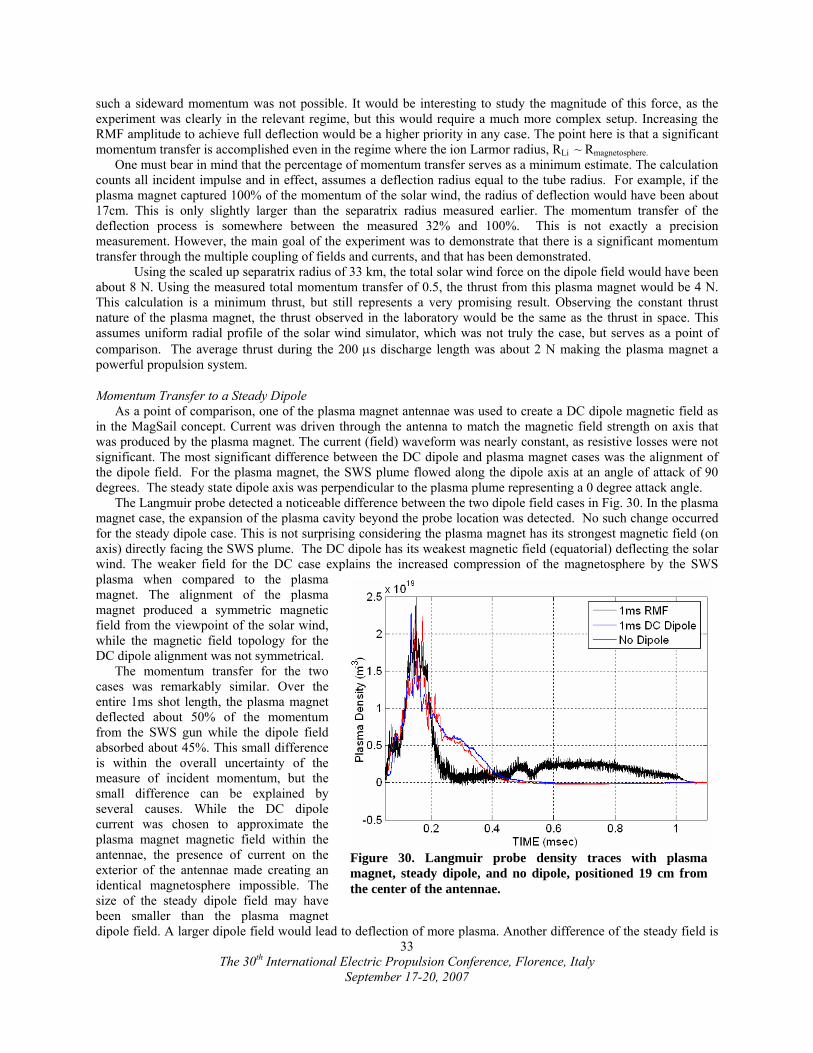
The 30th International Electric Propulsion Conference, Florence, Italy
September 17-20, 2007
33
such a sideward momentum was not possible. It would be interesting to study the magnitude of this force, as the experiment was clearly in the relevant regime, but this would require a much more complex setup. Increasing the RMF amplitude to achieve full deflection would be a higher priority in any case. The point here is that a significant momentum transfer is accomplished even in the regime where the ion Larmor radius, RLi ~ Rmagnetosphere.
One must bear in mind that the percentage of momentum transfer serves as a minimum estimate. The calculation counts all incident impulse and in effect, assumes a deflection radius equal to the tube radius. For example, if the plasma magnet captured 100% of the momentum of the solar wind, the radius of deflection would have been about 17cm. This is only slightly larger than the separatrix radius measured earlier. The momentum transfer of the deflection process is somewhere between the measured 32% and 100%. This is not exactly a precision measurement. However, the main goal of the experiment was to demonstrate that there is a significant momentum transfer through the multiple coupling of fields and currents, and that has been demonstrated.
Using the scaled up separatrix radius of 33 km, the total solar wind force on the dipole field would have been about 8 N. Using the measured total momentum transfer of 0.5, the thrust from this plasma magnet would be 4 N. This calculation is a minimum thrust, but still represents a very promising result. Observing the constant thrust nature of the plasma magnet, the thrust observed in the laboratory would be the same as the thrust in space. This assumes uniform radial profile of the solar wind simulator, which was not truly the case, but serves as a point of comparison. The average thrust during the 200 μs discharge length was about 2 N making the plasma magnet a powerful propulsion system.
Momentum Transfer to a Steady Dipole As a point of comparison, one of the plasma magnet antennae was used to create a DC dipole magnetic field as
in the MagSail concept. Current was driven through the antenna to match the magnetic field strength on axis that was produced by the plasma magnet. The current (field) waveform was nearly constant, as resistive losses were not significant. The most significant difference between the DC dipole and plasma magnet cases was the alignment of the dipole field. For the plasma magnet, the SWS plume flowed along the dipole axis at an angle of attack of 90 degrees. The steady state dipole axis was perpendicular to the plasma plume representing a 0 degree attack angle.
The Langmuir probe detected a noticeable difference between the two dipole field cases in Fig. 30. In the plasma magnet case, the expansion of the plasma cavity beyond the probe location was detected. No such change occurred for the steady dipole case. This is not surprising considering the plasma magnet has its strongest magnetic field (on axis) directly facing the SWS plume. The DC dipole has its weakest magnetic field (equatorial) deflecting the solar wind. The weaker field for the DC case explains the increased compression of the magnetosphere by the SWS plasma when compared to the plasma magnet. The alignment of the plasma magnet produced a symmetric magnetic field from the viewpoint of the solar wind, while the magnetic field topology for the DC dipole alignment was not symmetrical.
The momentum transfer for the two cases was remarkably similar. Over the entire 1ms shot length, the plasma magnet deflected about 50% of the momentum from the SWS gun while the dipole field absorbed about 45%. This small difference is within the overall uncertainty of the measure of incident momentum, but the small difference can be explained by several causes. While the DC dipole current was chosen to approximate the plasma magnet magnetic field within the antennae, the presence of current on the exterior of the antennae made creating an identical magnetosphere impossible. The size of the steady dipole field may have been smaller than the plasma magnet dipole field. A larger dipole field would lead to deflection of more plasma. Another difference of the steady field is
Figure 30. Langmuir probe density traces with plasma magnet, steady dipole, and no dipole, positioned 19 cm from the center of the antennae.

The 30th International Electric Propulsion Conference, Florence, Italy
September 17-20, 2007
34
its static nature. The decay of the SWS plume in time is analogous to rapid transit away from the sun. The DC field lines experience a decrease in compression as the plasma plume decays, and expand slightly. The plasma magnet however, experiences the very same field line expansion, but it is compounded by the expansion of the current carrying plasma sail. This plasma sail expansion could lead to slightly higher momentum transfer for the plasma magnet as the radius of deflection increases. However, the expansion of the plasma magnet occurred when the SWS plume was decaying, so for the period when the impulse of the plume was at its greatest, the plasma magnet was at its most compressed.
These effects could account for minor differences in this regime where the antennae size is comparable to the plasma sail size. In space the plasma sail would be significantly larger than the RMF antennae and lead to a much larger momentum transfer. Regardless of scaling, these results show that the difference in alignment of the dipole field is negligible when compared to the other uncertainties between the DC and RMF cases.
The interaction of the solar wind with the MagSail was modeled using MHD by Nashida et al20. Similar work was done using a kinetic model by Akita and Suzuki21. A useful parameter when evaluating the two treatments is the ratio of the ion Larmor radius to the scale size of the device. For rLi/r the device is large enough that the gyro orbits of the particles are negligible and MHD is appropriate. As already mentioned, when rLi/r ~ 1 kinetic effects become significant as it was in these experiments. The effective size of the interaction of the magnetosphere and the SWS is thus much reduced from the MHD calculations. These calculations are useful in that they provide insight into how the motion of the solar wind is affected by the magnetic field geometry.
In the numerical MHD simulations, the deflection of the solar wind was sensitive to the alignment of the dipole field. An attack angle of 90 degrees was found to produce the maximum drag coefficient with the angle 0 degrees slightly lower20. In these calculations the magnetosphere appears to be significantly larger on the sun facing side at 90 degrees than at 0 degrees, which agrees with experimental observations.
V. Summary of Experimental Results The plasma magnet is an revolutionary concept that has the potential to harness the kinetic energy of the solar
wind for space propulsion. The very low dynamic pressure of the solar wind requires a plasma sail size on the order of 10 km. A plasma magnet dipole field expanded to a scale on the order of tens of km would potentially provide thrust on the order of a few Newtons at powers in the megawatt range. The ability to create a plasma magnet, where the steady dipole field was provided solely by plasma currents was demonstrated at a magnitude and pressure capable of expansion to the requisite scale. The final step of actually creating a dynamic equilibrium with a solar wind source was also accomplished.
A modified MPD thruster was used as the solar wind simulator and the modified thruster was thoroughly characterized. The initial flow speed of the plume was found to be about 50 km/s. The impulse of the plume was measured to be on the order of 1 mN-s in the plane of the plasma magnet. Expansion of the magnetosphere and deflection of the plasma plume was detected by both a magnetic probe array as well as a Langmuir probe positioned within the magnetosphere. The plasma magnet was observed to contract and expand in response to changes in the SWS plasma flow demonstrating that a dynamic equilibrium in a flowing plasma can be maintained. The interception of the initial SWS plasma was used to bootstrap the initial inflation of the plasma magnet making for a propellantless propulsion device. A much expanded plasma magnet persisted long after the SWS pulse indicating an enhanced plasma confinement characteristic observed in plasmoids generated and sustained by RMF.
The plasma magnet was mounted on what in effect was a counter weighted ballistic pendulum, and placed in the solar wind source plasma stream. An optical displacement sensor was employed to track momentum transfer to the plasma magnet system. It was calibrated with a simple pendulum. The pendulum was arranged as an impact hammer in the range relevant range of the expected impulse bit from the pulsed plasma magnet and solar wind. After accounting for all sources of extraneous momentum transfer, the momentum transferred to the pendulum from deflection off the plasma magnetosphere was measured to be approximately one third of the total SWS plume across the entire tube radius. The actual transfer of momentum was more efficient, as the radius of deflection was significantly smaller than the tube radius. With this measurement, the transfer of momentum to the antennae structure coupled through the plasma current and RMF to the dipole magnetic field was validated. The average thrust during the 200 μs pulse length was 2 N. With a characteristic SWS flow speed the “jet” power observed was 1 MW. Higher power was limited by both the flow speed of the SWS that could be attained, as well as arcing limitations due to an antenna insulation issues. Additional enhancement of the deflection radius is expected as the system becomes more MHD-like (solar wind source ion Larmor radius less than the plasma magnet separatrix

The 30th International Electric Propulsion Conference, Florence, Italy
September 17-20, 2007
35
radius). The laboratory plasma magnet/SWS system tested was still in the kinetic regime where ion deflection was incomplete.
With the successful demonstration of thrust power at the MW level, a final large tank test or possibly even a space demonstration with a microsat should be undertaken. These experiments would provide the final confirmation of the scaling for a deep space mission.
Acknowledgments The author would like to thank the several students and staff that assisted in the construction, data taking, and
analysis during this study. In particular the author would like to thank Samuel Andreason for the design of much of the electronics and power systems, Louis Giersch for magnet design and analysis on the phase I experiments, and Adam Zeleske for assistance in the very difficult task of making the thrust measurement as well as the characterization of the SWS. This work was supported under a grant from the NASA Institute for Advanced Concepts (NIAC).
References 1Parks, G., Physics of Space Plasmas, Addison-Wesley Publishing Co., 1991. 2Winglee, R.M., Slough, J., Ziemba, T., and Goodson, A., “Mini-magnetospheric plasma propulsion: Tapping the energy of
the solar wind for spacecraft propulsion”, J. Geophys. Res., 105 21067 (1999). 3G. Khazanov et al. “Fundamentals of the plasma sail concept: MHD and kinetic studies”, AIAA Joint Propulsion Conference
2003 4Hugrass, W.N., I.R. Jones and M.G.R. Phillips, “An experimental investigation of current production by means of a rotating
magnetic field”, J. Plasma Physics 26, 465 (1981) 5Slough, J.T. and Miller, K.E., “Flux generation and sustainment of a Field Reversed Configuration (FRC) with Rotating
Magnetic Field (RMF) current drive”, Physics of Plasmas, 7, 1495 (2000) 6Slough, J.T. and Miller, K.E., “Enhanced Confinement and Stability of a Field Reversed Configuration with Rotating
Magnetic Field current drive”, Phys. Rev. Lett. 85 1444 (2000) 7Zubrin, R.M. and Andrews, D.G., “Magnetic Sails and Interplanetary Travel”, Journal of Spacecraft, 28 197 (1991). 8 Winglee, r.M., Slough, J.T., Ziemba, T., and Goodson, A., “Mini-magnetospheric plasma propulsion: High speed
propulsion sailing the solar wind”, Space Technology and Applications (2000) 9John Slough, “High Beta Plasma for Inflation of a Dipolar Magnetic Field as a Magnetic Sail”, Proceedings of the IEPC
Conference, Oct. 14-19, 2001, Pasedena CA. 10Slough, J.T., and Andreason, S.P. “High field RMF FRC experiments on STX-HF”, Submitted to Physics of Plasmas. 11Krasheninnokov, S.I., Catto, J.J., Hazeltine, R.D., “Magnetic Dipole Equilibrium Solution at Finite Plasma Pressure”,
Physical Review Letters, 82 2689 (1999). 12Gernier, D.T., Kesner, J., and Mauel, M.E., “Magnetohydrodynamic stability in a levitated dipole”, Physics of Plasmas, 6
3431 (1999) 13Fiksel, G., et. al, “High current plasma electron emitter”, Plasma Sources Sci. Technol. 5, 78 (1996). 14E.A. Cubbin, J.K. Ziemer, E.Y. Choueiri, and R.G. Jahn, “Pulsed thrust measurements using laser interferometry”, Rev.
Sci. Instruments, 68 2339 (1997). 15D. Winske and N. Omidi, “Plasma expansion in the presence of a dipole magnetic field”, Physics of Plasmas, 12, July,
2005. 16H. Nishida et al., “Verification of Momentum Transfer Process on Magnetic Sail Using MHD Model”, AIAA 2005-4463,
41st AIAA/ASME/SAE/ASEE Joint Propulsion Conference and Exhibit, 10-13 July 2005, Tucson, Arizona. 17Chen, F. (1984). Introduction to Plasma Physics and Controlled Fusion. New York: Plenum Press. 18Uribarri, Luke & Choueiri, E.Y. “The onset of voltage hash and its relationship to anode spots in magnetoplasmadynamic
thrusters”. IEPC 2005 20Nashida, H. et al. (2005). Verification of momentum transfer process on magnetic sail using MHD model. JPC 2005. 21Akita, Daisuke and Suzuki, Kojiro (2005) Kinetic analysis on plasma flow of solar wind around magnetic sail. JPC 2005