matlabtm simulink - tÜbİtakjournals.tubitak.gov.tr/elektrik/issues/elk-12-20-4/elk-20-4-3...a...
TRANSCRIPT

Turk J Elec Eng & Comp Sci, Vol.20, No.4, 2012, c© TUBITAK
doi:10.3906/elk-1011-928
A novel three-phase transformer hysteresis model in
MATLABTM Simulink
Okan OZGONENEL1,∗, Kamil Rıfat Irfan GUNEY2, Omer USTA3, Hasan DIRIK1
1Department of Electrical & Electronics Engineering, Ondokuz Mayıs University,55139 Kurupelit, Samsun-TURKEY
e-mails: [email protected], hasan [email protected] Faculty, Acıbadem University, Uskudar,
34662 Istanbul-TURKEYe-mail: [email protected]
3Department of Electrical Engineering, Istanbul Technical University,Maslak, Istanbul-TURKEY
e-mail: hasan [email protected]
Received: 10.11.2010
Abstract
This paper presents a new transformer model displaying hysteresis using the MATLABTM Simulink
environment. The proposed model displays a complete scheme for the simulation of 3-phase transformers.
The new model is mainly based on the transmission line model and the Jiles-Atherton model of a power
system using lumped parameters. Jiles-Atherton model parameters were determined by curve fitting and
numerical optimization iteration. The developed model is particularly suitable for fault analysis and protective
relaying studies under harmonic conditions where the transformer is driven into the nonlinear regime. The
performance of the method was evaluated by both theorical and experimental data.
Key Words: Transformer modeling, hysteresis, Jiles-Atherton
1. Introduction
The power transformer is one of the most important elements of power systems, since the continuity oftransformer operation has vital importance in maintaining the reliability of the power supply. Therefore,various modeling schemes have been developed over the decades to provide a proper protective method for thetransformers, and there have been many attempts to precisely estimate the hysteresis behavior of ferromagneticmaterials, especially in the transformer’s core [1].
The development and validation of protective algorithms for the transformers requires the preliminarydetermination of the transformer model. The model used is required to simulate the power system’s normal
∗Corresponding author: Department of Electrical & Electronics Engineering, Ondokuz Mayıs University, 55139 Kurupelit,Samsun-TURKEY
479

Turk J Elec Eng & Comp Sci, Vol.20, No.4, 2012
and faulted conditions and to estimate the behavior of the protection algorithm under abnormal conditions.In particular, it must allow for the simulation of internal and external fault conditions. Most of the presentelectromagnetic transient programs are able to accurately simulate some of the phenomena occurring in thetransformer, like magnetizing inrush current, excitation current, and transformer saturation [2]. However, the
implementations of the present monitoring methods [3,4] tend to cost too much to be applied to distributiontransformers. Such analysis also usually requires commercial software such as FEMLAB, MAGNET, or ANSYSMaxwell. However, most of the present simulation programs are not able to properly simulate the hysteresischaracteristic of the core material [5].
This paper presents a 3-phase transformer model displaying hysteresis based on Jiles-Atherton (J-A)magnetization with a modified Langevin function and determination of model parameters; it is an extended
version of [1]. The nonlinear behavior of the transformer’s core was modeled using the MATLABTM Simulink
environment. The proposed model is based on the transmission line model (TLM) method for simulatingtransformers, which can consider nonlinear hysteresis. To validate the proposed technique, a 3-phase, 2-windinglaboratory-type transformer was modeled using the TLM method including the J-A technique with parameterestimation. The TLM method converts a second-order circuit into a first-order one, which simplifies the solutionof the circuit at any discrete time. In addition to this, it facilitates the incorporation of time-dependent modelssuch as the J-A model, which is described in Section 2. The proposed modeling technique is suitable for modelingtransformer-related phenomena such as magnetizing inrush, internal faults, and loading conditions.
2. Three-phase, two-winding transformer model
The TLM method was first developed in the early 1970s for modeling 2-dimensional field problems. Sincethen, it has been extended to cover 3-dimensional problems and circuit simulations. For circuit simulation, theTLM method can be used to develop a discrete circuit model directly from the system without setting up anyintegro-differential equations. The TLM algorithm is discrete in nature and ideally suited for implementationon computer-based systems [6].
The hysteresis specs of the transformer are based on the J-A technique in TLM simulations. The J-A technique describes the relationship between magnetic moment M and magnetic field intensity H usingthe current physical theories of magnetic domains in ferromagnetic materials [7], and it is able to presenta possible anisotropic steel behavior in transformers. The J-A model requires the following input parameters:magnetization saturation, thermal energy parameter, domain flexing constant, domain anisotropy constant, andinterdomain coupling parameter. These are not parameters that transformer manufacturers or manufacturersof transformer magnetic material can provide for users. In fact, they cannot even be determined directlythrough measurements. The various core hysteresis parameters required in this model are theorical and can becalculated from experimental measurements of coercivity, remanence, saturation flux density, initial anhystereticsusceptibility, initial normal susceptibility, and the maximum differential susceptibility [8]. Moreover, the J-Amodel requires little memory storage, as its status is totally described by only 5 parameters. On the otherhand, convergence problems may be encountered in the identification of these parameters by using iterativeprocedures. More details about the J-A technique can also be found in [9-11].
Conversion between the B-H loop and an M-H loop is straightforward and is calculated using Eq. (1).
B = μ0(H + M) (1)
480

OZGONENEL, GUNEY, USTA, DIRIK: A novel three-phase transformer hysteresis model in...,
The J-A hysteresis model decomposes the whole magnetization M into the reversible component Mrev
and the irreversible component Mirr [12].
M = Mrev + Mirr (2a)
Its current-related equation is given in Eq. (2b).
Im = Irev + Iirr (2b)
The reversible component is defined as in Eq. (3).
Mrev = c(Man − Mirr) (3a)
Its current-related equation is given in Eq. (3b).
Irev = c(Ian − Iirr) (3b)
Man is the anhysteretic magnetization provided by the Langevin equation. The magnetization relationshipbetween B and H is replaced by the anhysteretic magnetization curve between H and M as follows:
Man = Ms.f(He), (4)
where He = H + αM and is called the Weiss effective field. This is linked with magnetic field intensity H bythe modified Langevin function in Eq. (5) and the differential equation in Eq. (6).
Man = Ms
(coth
H + αM
a− a
H + αM
)(5a)
Its current-related equation is given in Eq. (5b).
Ian = Is
(coth(
IL + αIm
a− a
IL + αIm
)(5b)
dMirr
dH=
δm(Man − Mirr)kδ − α(Man − Mirr)
(6a)
Its current-related equation is given in Eq. (6b).
dIirr
dIL=
δm(Ian − Iirr)kδ − α(Ian − Iirr)
, (6b)
where δm and δ are given by:
δm =
⎧⎪⎪⎨⎪⎪⎩
1 : IF dHdt > 0 and Man > Mirr
1 : IF dHdt < 0 and Man < Mirr
0:otherwise
. (7a)
481

Turk J Elec Eng & Comp Sci, Vol.20, No.4, 2012
Its current related equation is given in Eq. (7b).
δm =
⎧⎪⎪⎨⎪⎪⎩
1 : IF dIL
dt> 0 and Ian > Iirr
1 : IF dIL
dt < 0 and Ian < Iirr
0 : otherwise
(7b)
δ =
⎧⎨⎩
1 : IF dHdt
> 0
1 : IF dHdt
< 0(8a)
Its current-related equation is given in Eq. (8b).
δ =
⎧⎨⎩
1 : IF dIL
dt> 0
1 : IF dIL
dt < 0(8b)
a, α, c, k, and Ms are the parameters of the model, where a is a form factor, α is the interaction between thedomains, c is the coefficient of reversibility of the movement of the walls, k represents the hysteresis losses,and Ms is the saturation magnetization. Numerical iterative techniques such as least-square curve fittingquasi-Newton approaches are used to determine these parameters.
3. Parameter estimation
The literature presents several step-by-step methods for the identification of the J-A model parameters fromexperimental B-H loops, which are based on the physical meaning of the parameters. Among them, random anddeterministic searches of the J-A model parameters [13], particle swarm optimization [14], the simplex method
and simulated annealing algorithm [15], estimations by using a global optimization technique known as “branch
and bound” [16], and usage of the genetic algorithm for parameter estimation [17] are the recent studies in theliterature. In this work, parameters are extracted using a least-square method, imposing the condition of thelocal minimum, and solving the equations using Newton’s method.
3.1. Anhysteretic susceptibility
The anhysteretic susceptibility at the origin can be used to define a relationship among Ms , a , and α [18].
Xan =(
dMan
dH
)M=0,H=0
(9a)
α =Ms
3
(1
Xan+ α
)(9b)
Its current-related equation is given in Eqs. (9b) and (10b).
Xan =(
dIan
dIL
)Im=0,IL=0
(10a)
α =Is
3
(1
Xan+ α
)(10b)
482

OZGONENEL, GUNEY, USTA, DIRIK: A novel three-phase transformer hysteresis model in...,
3.2. Initial susceptibility
The reversible magnetization component is expressed via parameter c in the hysteresis equation, Eq. (6a),defined by:
xini =(
dM
dH
)M=0,H=0
=cMs
3α. (11a)
Its current-related equation is given in Eq. (11b).
xini =(
dIm
dIL
)Im=0,IL=0
=cIs
3α(11b)
3.3. Coercivity
The hysteresis loss parameter k can be determined from coercivity Hc and the differential susceptibility atcoercive point Xan(Hc).
k =Man(Hc)
1 − c
⎡⎣α +
1
X(Hc) −(
c1−c
)dMdH
⎤⎦ (12a)
Its current-related equation is given in Eq. (12b).
k =Ian(Ic)1 − c
⎡⎣α +
1
X(Ic) −(
c1−c
)dIm
dIL
⎤⎦ (12b)
3.4. Remanence
The coupling parameter α can be determined independently if it is known by using remanence magnetizationMr and the differential susceptibility at remanence.
Mr = Man(Mr) +k
aa−c + k
X(Mr)−c dMdH
(13)
4. Modeling procedure
Figure 1 shows the transformer core type under modeling consideration. In Figure 1, Na and Nb represent thenumber of turns of primary and secondary windings, respectively. Lowercase subscripts represent the primaryside parameters, while capitalized subscripts represent secondary side parameters. The linear transformer modelis shown in Figure 2.
The main modeling equations, such as Va−b−c , VA−B−C (primary and secondary voltages, respectively),
and Ma−b−c (magnetization intensities of the phases), are defined in Eq. (14), respectively. For simplicity, onlyphase a and phase A equations are explained here.
Va =LaadIa
dt+
LaAdIA
dt+ Na
LmdIma
dt
VA =LAAdIAa
dt+
LaAdIa
dt+ NA
LmdIma
dt
(14)
483

Turk J Elec Eng & Comp Sci, Vol.20, No.4, 2012
Va Vb Vc
Ia I b I c
VA VB VC
IA IB I C
1Φ 2Φ 3Φ
Figure 1. A 3-phase, 2-winding star/star-connected transformer.
Va
Vb
Vc
Ia
Ib
Ic
iaaV2
ibbV2
iccV2
aaZ
bbZ
ccZ
+ -
+ -
+ -
aAV
bBV
cCV
AaV
BbV
CcV
AAZ
BBZ
CCZ
iAAV2
iBBV2
iCCV2
VA
VB
VC
IA
IB
IC
+ -
+ -
+ -
- +
- +
- +
- +
- +
- +
iaAV2
aAZaAV
AI
ibBV2
bBZbBV
BI
icCV2
cCZcCV
CI
iAaV2
AaZAaV
aI
iBbV2
BbZBbV
bI
iCcV2
CcZCcV
cI
Figure 2. Linear modeling of the 3-phase, 2-winding transformer.
Here, Laa = μ0N2aA
l , LAA = μ0N2AA
l , Lm = μ0Al , A is the cross-sectional area in square meters, and l is the
length of the magnetic path in meters. These are initially calculated as the simulation starts. The characteristicimpedances of the primary and secondary sides are then calculated as follows:
Zaa = 2Laa
dt ,
ZAA = 2LAA
dt .(15)
Similarly, the characteristic impedances of the magnetizing branches are calculated using the following equations.
LaA = (μ0NaNAA)/l
ZaA = 2LaA/dt(16)
484

OZGONENEL, GUNEY, USTA, DIRIK: A novel three-phase transformer hysteresis model in...,
Leakage inductances and related characteristic impedances are calculated using Eq. (10).
ZLaS = 2LaS/dt
ZLAS = 2LAS/dt(17)
ZLaS and ZLAS are the leakage characteristic impedances of the primary and secondary sides, respectively.For a lossless linear transformer, the mutual TLM voltages are defined in Eq. (18) and Eq. (14) as follows:
VaA = ZaAIA + 2V iaA, (18)
VAa = ZAaIa + 2V iAa, (19)
where ZaA = 2LaA
dt and dt is the sampling interval.
After these calculation steps, the primary and secondary currents, Ia and IA , are calculated using Eqs.(20) and (21).
ZaaIa + ZaAIA = Va − 2(V iaa + V i
aA) (20)
ZaAIa + ZAAIA = −2(V iAa + V i
AA) (21)
Here, Zaa = 2Laa
dt.
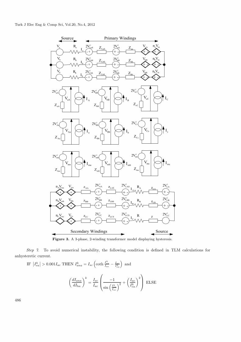
In Eq. (14), Va is the source voltage of phase a. The calculations are repeated until the end of thesimulation time. Figure 3 shows a 3-phase, 2-winding transformer model displaying hysteresis.
The required calculations for the hysteresis model of a 3-phase transformer are somewhat complicatedin the linear model. To have a complete model, source and load impedances are added to the simulation. Tosimplify the whole procedure, the equations are given for only phase a here.
The whole calculation procedure, step by step, is explained below.
Step 1. V ka is obtained, k = 1, 2, 3, ...N . N is the number of samples.
Step 2. Phase-neutral voltage is calculated as:
V ksa = V k
a + RaIka ,
where Ra is the source resistance.Step 3. J-A calculations are begun from this step. Total ampere turns is calculated as:
Ikha = NaIk
a + NAIkA.
Step 4. The exciting current is calculated as:
Ikea = Ik
ha + αIkma.
Step 5. Updating of the total ampere turns of the phases as:
dIk+1ha = Ik
ha − (NaIk−1a + NAIk−1
A ).
Step 6. Directional flag is defined according to dkha as:
IF dkha < 0 THEN Δk
a = −1 ELSE Δka = 1.
485
Turk J Elec Eng & Comp Sci, Vol.20, No.4, 2012
aV+ -- +
iaAV2
aAZaAV
AI
ibBV2
bBZbBV
BI
icCV2
cCZcCV
CI
iAaV2
AaZAaV
aI
iBbV2
BbZBbV
bI
iCcV2
CcZCcV
cI
aRaI
iLaSV2
LaSZi
aAV2aaZ
+ - + -aAV maVn
Source Primary Windings
bV
+ -- +bR
bIi
LbSV2LbSZ
ibBV2
bbZ+ - + -
bBV mbVn
bV
+ -- +bR
bIi
LbSV2LbSZ
ibBV2
bbZ+ - + -
bBV mbVn
imaV2
maZmaV
maI
imbV2
mbZmbV
mbI
imcV2
mcZmcV
mcI
maAVn AaVAAz
iAAV2
LASzLAzAR
- + - +
iLAV2i
LASV2
+ -+ -- + AI
mbBVn BbVBBz
iBBV2
LBSzLBzBR
- + - +
iLBV2i
LBSV2
+ -+ -- + BI
mcCVn CcVCCz
iCCV2
LCSzLC
zC
R- + - +
iLCV2i
LCSV2
+ -+ -- + CI
SourceSecondary Windings
Figure 3. A 3-phase, 2-winding transformer model displaying hysteresis.
Step 7. To avoid numerical instability, the following condition is defined in TLM calculations foranhysteretic current.
IF∣∣Ik
ea
∣∣ > 0.001Iac THEN Ikana = Isc
(coth Ik
ea
Iac− Iac
Ikea
)and
(dIana
dIha
)k
=Isc
Iac
⎛⎜⎝ −1
sin(
Ikea
Iac
)2 +(
Iac
Ikea
)2
⎞⎟⎠ ELSE
486
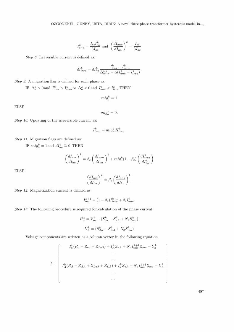
OZGONENEL, GUNEY, USTA, DIRIK: A novel three-phase transformer hysteresis model in...,
Ikana =
IscIkea
3Iacand
(dIana
dIha
)k
=Isc
3Iac
Step 8. Irreversible current is defined as:
dIkirra = dIk
ha
Ikana − Ik
irra
ΔkaIcc − α(Ik
ana − Ikirra)
.
Step 9. A migration flag is defined for each phase as:
IF Δka > 0and Ik
ana > Ikirra or Δk
a < 0and Ikana < Ik
irra THEN
migka = 1
ELSEmigk
a = 0.
Step 10. Updating of the irreversible current as:
Ikirra = migk
adIkirra.
Step 11. Migration flags are defined as:
IF migka = 1and dIk
ha∼= 0 THEN
(dIma
dIha
)k
= βc
(dIana
dIha
)k
+ migka(1 − βc)
(dIk
irra
dIkha
)
ELSE (dIma
dIha
)k
= βc
(dIana
dIha
)k
.
Step 12. Magnetization current is defined as:
Ik+1ma = (1 − βc)Ik+1
irra + βcIkana.
Step 13. The following procedure is required for calculation of the phase current.
Uka = V k
sa − (Skaa − Sk
aA + NaSkma)
UkA = (Sk
Aa − SkAA + NaSk
ma)
Voltage components are written as a column vector in the following equation.
f =
⎡⎢⎢⎢⎢⎢⎢⎢⎢⎢⎢⎣
Ika (Ra + Zaa + ZLaS) + Ik
AZaA + NaIk+1ma Zma − Uk
a
...
...
IkA(RA + ZAA + ZLaS + ZLA) + Ik
a ZaA + NaIk+1ma Zma − Uk
A
...
...
⎤⎥⎥⎥⎥⎥⎥⎥⎥⎥⎥⎦
487

Turk J Elec Eng & Comp Sci, Vol.20, No.4, 2012
The Jacobian matrix is defined as below.
J =
[J11 J12
J21 J22
]
J11 =
⎡⎢⎢⎣
Ra + ZLaS + Zaa
(1 +
(dIma
dIha
)k)
0 0
0 ... 0
0 0 ...
⎤⎥⎥⎦
J12 =
⎡⎢⎢⎣
ZaA
(1 +
(dIma
dIha
)k)
0 0
0 ... 0
0 0 ...
⎤⎥⎥⎦
J21 = J12J22 =
⎡⎢⎢⎣
RA + ZLAS + ZLA + ZAA
(1 +
(dIma
dIha
)k)
0 0
0 ... 0
0 0 ...
⎤⎥⎥⎦
The Newton-Raphson iteration method is applied to calculate the next sample of phase currents.
⎡⎢⎢⎢⎢⎢⎢⎢⎢⎢⎣
Ik+1a
...
...
Ik+1A
...
...
⎤⎥⎥⎥⎥⎥⎥⎥⎥⎥⎦
=
⎡⎢⎢⎢⎢⎢⎢⎢⎢⎢⎣
Ika
...
...
IkA
...
...
⎤⎥⎥⎥⎥⎥⎥⎥⎥⎥⎦− J−1f
Step 14. Updating of the magnetizing current is defined as:
fma = Ik+1a (Ra + Zaa) + Ik+1
A ZaA + NaIk+1ma Zma − Uk
a
Ik+1ma = Ik
ma − fma
NaZma.
Step 15. This step includes the updating procedures for accumulator values.
Sk+1aa = −(Sk
aa + 2Ik+1a Zaa)
Sk+1Aa = −(Sk
Aa + 2Ik+1a ZaA)
Sk+1AA = −(Sk
AA + 2Ik+1A ZAA)
Sk+1ma = −(Sk
ma + 2Ik+1ma Zma)
Step 16. This step includes the calculation of simulation outcomes.
ψa = dtV k
a − V k−1a
2
488

OZGONENEL, GUNEY, USTA, DIRIK: A novel three-phase transformer hysteresis model in...,
Bka =
μ0
l(NaIk+1
a + NAIk+1A + Ik+1
ma )
Hka =
(NaIk+1a + NAIk+1
A )l
These equations are executed in the MATLABTM Simulink environment. The simulation parameters ofthe modeled transformer can easily be changed. The user can easily change the required parameters by doubleclicking each block inside the model. The main TLM transformer block is suitable for implementing differenttypes of 3-phase connections on both sides. The “powergui” option in the proposed model is used for waveformanalysis. Basically, the TLM model consists of current-voltage measurement units, J-A implementation units,and a Jacobean matrix calculation module (subsystem4) for each phase.
Figure 4 shows the overall flowchart for a single phase.
Initial CalculationsCalculate all characteristic impedances, (Zaa, ZAA), (ZaA ), (Zma), (ZLaS, ZLAS)Calculate saturation current, and anhysteretic current and coercive current, (Isc, Iac, Icc)
Define primary and secondary currents as zero initially (Ia, IA=0)Define initial accumulator values as zero (S aa, S aA , S Aa, S AA, Sma=0)
Read the primary voltage (Va)
Calculate magnetizing current by Jiles -Atherton method (Im)
Calculate load resistance and inductance by using short window algorithm (R y, Ly)
Calculate primary and secondary currents (Ia, IA)
Update accumulator values as zero (S aa, S aA , S Aa, S AA, Sma)
Calculate simulation outputs (B, H)
Figure 4. A complete flowchart for a single-phase modeling procedure.
5. Model verification
To demonstrate the validity of the modeling procedure, a 3-phase, 2-winding test transformer was used in thelaboratory and modeled using the TLM method described in Section 2. The transformer was loaded witha star-connected R-L load to simulate normal and faulted conditions. As seen in Figure 4, the user defines
the following parameters: source frequency, magnetic path length (m), core area (m2), number of turns for
primary and secondary windings, saturation magnetization (m−1), anhysteretic form factor (m−1), interdomain
coupling coefficient, coercive field magnitude (m−1), magnetization weight factor, permeability of free space,leakage inductances of primary and windings, source resistors, load impedances, and load factor.
The performance of the proposed technique was evaluated by root mean square error (RMSE). Figure 5shows the primary phase currents obtained using the TLM and J-A models.
In this particular example, the 3-phase source voltage is defined as VpeakSin(wt + φ)(1 − e−15t).
489

Turk J Elec Eng & Comp Sci, Vol.20, No.4, 2012
Figure 6 shows the B-H curve of phase a.
0 0.02 0.04 0.06 0.08 0.1 0.12 0.14 0.16 0.18 0.2-20
-10
0
10
20
Time (s)
Cur
rent
(m
A)
iabic
-400 -300 -200 -100 0 100 200 300 400-1.5
-1
-0.5
0
0.5
1
1.5
Ha
Ba
Real curveSimulated curve
Figure 5. Simulated primary phase currents ( ia, ib, ic) . Figure 6. Real and simulated (best-fit) B-H curve of the
transformer for phase A. RMSE for H is 7.9803, for B is
5.8065 × 10⁻⁴ .
To simulate the magnetizing inrush condition in the J-A model, a (zero crossing) source voltage of√
2∗ 220 ∗ sin(w ∗ t) is applied. Figure 7 shows the typical inrush current of the modeled transformer and Figure8 shows the real and simulated B-H curve of the transformer.
0 0.02 0.04 0.06 0.08 0.1 0.12 0.14-2
0
2
4
6
8
10
Time (s)
Cur
rent
(A
)
Real curveSimulated curve
-600 -400 -200 0 200 400 600 800 1000 1200 1400
-0.5
0
0.5
1
H−Magnetic field intensity A/m
B−
Mag
netic
flu
x de
nsity
T
Real curveSimulated Curve
Figure 7. Real and simulated inrush currents of the
modeled transformer for phase A. RMSE = 0.0029.
Figure 8. Real and simulated B-H curve of the trans-
former during inrush phenomenon for phase A. RMSE for
Ha is 34.94, for B is 0.0144.
6. Conclusion
This paper introduces a time domain model of a 3-phase, 2-winding transformer with nonlinear and hysteretic
behavior. It is a complete 3-phase transformer model in the MATLABTM Simulink environment. The user caneasily change the parameters by double clicking the “TLM Model of 3-Phase Transformer Model” block. Thehysteretic model using the modified Langevin function is based on the J-A model of ferromagnetic hysteresis.The simulation results produce an acceptable transformer transient response and show that the proposed overalltechnique is ideal for simulating 3-phase transformers.
The proposed modeling technique displaying hysteresis is suitable for most types of 3-phase, 2-windingstransformers. The suggested modeling technique is also able to simulate the transformers during single ormultiple internal faults.
490

OZGONENEL, GUNEY, USTA, DIRIK: A novel three-phase transformer hysteresis model in...,
Appendix
Data for test transformer:U1 /U2 = 380/220 V, star/star-connected
f = 50 Hz
B = 1 TS = 1 kVAlm = 24.10−3 m, magnetic path length
a = 454.10−6 m2 , core areaNa = 565, primary turns
NA = 255, secondary turns
Ms = 170000 m−1 , saturation magnetization
Ha = 42 m−1 , anhysteretic form factor
α = 8.10−6 , interdomain coupling coefficient
Hc = 78 A Tm−1 , coercive field magnitude
βc = 0.55, magnetization weighting factorRa , Rb , Rc = 10 Ω, source resistances
μ0 = 4π × 10−7 H m−1 , permeability of the free space
Acknowledgment
This work was supported by TUBITAK-2219, a postdoctoral study at The University of Nottingham, UK.
References
[1] D.W.P Thomas, J. Paul, O. Ozgonenel, C. Christopoulos, “Time-domain simulation of nonlinear transformers
displaying hysteresis”, IEEE Transactions on Magnetics, Vol. 42, pp. 1820-1827, 2006.
[2] P. Bastard, P. Bertrand, M. Mevnier, “A transformer model for winding fault studies”, IEEE Transactions on Power
Delivery, Vol. 9, pp. 690-699, 1994.
[3] T. Leibfried, K. Feser, “Monitoring of power transformers using the transfer function method”, IEEE Transactions
on Power Delivery, Vol. 14, pp. 1333-1341, 1999.
[4] A.I. Megahed, “A model for simulating internal earth faults in transformers”, 7th International Conference on
Developments in Power Systems Protection, pp. 359-362, 2001.
[5] H. Wang, K.L. Butler, “Finite element analysis of internal winding faults in distribution transformers”, IEEE
Transactions on Power Delivery, Vol. 16, pp. 442-427, 2001.
[6] S.Y.R. Hui, C. Christopoulos, “Discrete transform technique for solving nonlinear circuits and equations”, IEE
Proceedings A, Vol. 139, pp. 321-328, 1992.
[7] D.C. Jiles, D.L. Atherton, “Ferromagnetic hysteresis,” IEEE Transactions on Magnetics, Vol. MAG-19, pp. 2183-
2185, 1983.
491

Turk J Elec Eng & Comp Sci, Vol.20, No.4, 2012
[8] S. Cundeva, “A transformer model based on the Jiles-Atherton theory of ferromagnetic hysteresis”, Serbian Journal
of Electrical Engineering, Vol. 5, pp. 21-30, 2008.
[9] X. Wang, M. Sumner, D.W.P. Thomas, “Simulation of single phase nonlinear and hysteretic transformer with
internal faults”, Power Systems Conference and Exposition, pp. 1075-1080, 2006.
[10] X. Wang, D.W.P. Thomas, M. Sumner, J. Paul, S.H.L. Cabral, “Characteristics of Jiles-Atherton model parameters
and their application to transformer inrush current simulation”, IEEE Transactions on Magnetics, Vol. 44, pp. 340-
345, 2008.
[11] K. Chwastek, J. Szcyglowski, “Modelling dynamic hysteresis loops in steel sheets”, COMPEL: The International
Journal for Computation and Mathematics in Electrical & Electronic Engineering, Vol. 28, pp. 603-612, 2009.
[12] X. Wang, D.W.P. Thomas, M. Sumner, J. Paul, S.H.L. Cabral, “Numerical determination of Jiles-Atherton model
parameters”, COMPEL: The International Journal for Computation and Mathematics in Electrical & Electronic
Engineering, Vol. 28, pp. 493-503, 2009.
[13] E. Del Moral Hernandez, C.S. Muranaka, J.R. Cardoso, “Identification of the Jiles-Atherton model parameters
using random and deterministic searches”, Elsevier Physica B, Vol. 275, pp. 212-215, 2000.
[14] R. Marison, R. Scorretti, N. Siauve, “Identification of Jiles-Atherton model parameters using particle swarm
optimization”, IEEE Transactions on Magnetics, Vol. 44, pp. 894-897, 2008.
[15] J. Zeng, B. Bai, “Evaluation of Jiles-Atherton hysteresis model’s parameters using mix of simplex method and
simulated annealing method”, International Conference on Electrical Machines and Systems, pp. 4033-4036, 2008.
[16] K. Chwastek, J. Szcyglowski, “An alternative method to estimate the parameters of Jiles-Atherton model”, Journal
of Magnetism and Magnetic Materials, Vol. 314, pp. 47-51, 2007.
[17] B. Zidaric, D. Miljavec, “J-A hysteresis model parameters estimation using GA”, Advances in Electrical and
Electronic Engineering, Vol. 4, pp. 174-177, 2005.
[18] M. Morjaoui, B. Boudjema, M. Chabane, R. Daira, “Qualitative modeling for ferromagnetic hysteresis cycle”, World
Academy of Science, Engineering and Technology, Vol. 36, pp. 88-94, 2007.
492