frobenius splitting for schubert …yisun.io/notes/frobsplit.pdffrobenius splitting for schubert...

FROBENIUS SPLITTING FOR SCHUBERT VARIETIES

YI SUN

Abstract. This thesis presents an expository account of the use of Frobenius splitting techniques in thestudy of Schubert varieties. After developing the basic theory of Frobenius splitting, we show that the

Schubert and Bott-Samelson varieties are split and use this to derive geometric consequences in arbitrarycharacteristic. The main result highlighted is that Schubert varieties are normal, Cohen-Macaulay, and have

rational resolutions. In addition, we give a proof of the Demazure character formula.

Contents

1. Introduction 11.1. Motivation 11.2. Conventions and notations 11.3. Organization and references 21.4. Acknowledgments 22. The Schubert and Bott-Samelson varieties 22.1. Notations and preliminaries 22.2. Flag and Schubert varieties 32.3. The Bott-Samelson variety 32.4. Line bundles on the Schubert and Bott-Samelson varieties 73. Frobenius splitting 103.1. Basic properties of Frobenius splitting 103.2. A splitting criterion for smooth projective varieties 133.3. Splitting and cohomology vanishing 154. A key cohomology vanishing result on the Bott-Samelson variety 164.1. Splitting of the Bott-Samelson and Schubert varieties 174.2. Proof of the vanishing result 174.3. Passing to characteristic 0 205. Proofs of the main results 215.1. Schubert varieties are normal and Cohen-Macaulay 215.2. Demazure character formula 22Appendix A. Duality for the Frobenius morphism on smooth varieties 26References 28

Date: March 22, 2010.

0

FROBENIUS SPLITTING FOR SCHUBERT VARIETIES 1

1. Introduction

1.1. Motivation. Let G be a semi-simple algebraic group over an algebraically closed field k with fixedBorel subgroup B containing a maximal torus T . When k has characteristic 0, the Borel-Weil-Bott Theoremallows one to recover the representation theory of G from the geometry of the flag variety G/B. Moreprecisely, to each integral weight λ is associated a certain line bundle L(λ) on G/B, on which all but onecohomology group vanishes. This non-vanishing cohomology group is then the irreducible representationof G with a specified highest weight, for which the Weyl character formula provides an explicit characterdecomposition.

The flag variety is classically equipped with a decomposition into Schubert varieties coming from theBruhat decomposition. Given the strength of the results on the flag variety, one might hope to find refine-ments of them on the smaller Schubert varieties. Indeed, the geometry of the Schubert varieties is quitenice; they are normal, Cohen-Macaulay varieties admitting a rational resolution of singularities. As a result,we have many results of a similar flavor to those present for the flag variety – the pullbacks of the linebundles L(λ) have vanishing higher cohomology, and we may recover a character formula for their uniquenon-vanishing cohomology group, though it is now only B-module rather than a G-module.

This is quite a beautiful picture; however, it comes with a caveat. If we allow k to have characteristicp, many of these results become much weaker, as many complex analytic tools may no longer be used. Inparticular, for an arbitrary integral weight λ, it may not be the case that Hi(G/B,L(λ)) is non-zero for aunique value of i. If we restrict λ to be a dominant weight, these vanishing theorems can be salvaged, buteven then the unique non-zero cohomology group may no longer be an irreducible representation of G. 1

The situation for Schubert varieties is similarly muddled. Our advertised results will remain true overarbitrary characteristic, but many of the geometric techniques used to obtain them originally are validonly in characteristic 0. However, in [MR], Mehta and Ramanathan were able to bypass many of thedifficulties by introducing the new notion of a Frobenius split scheme, which ironically is valid only inpositive characteristic. This property, define as the splitting of the absolute Frobenius homomorphism ona scheme, captures a type of geometric information about a scheme; for instance, Frobenius split schemesare reduced and all higher cohomologies of ample line bundles on them vanish. This idea is just enough toobtain in positive characteristic many of the nice results known in characteristic 0; in fact, it will even implythe original characteristic 0 results by semi-continuity!

The purpose of this thesis is to give an expository account of the use of these Frobenius splitting techniquesin the context of Schubert varieties. In practice, this will be require a significant amount of additional input.It is difficult to prove directly that the Schubert varieties are Frobenius split, as they are highly singular.Thus, we consider instead an explicit desingularization, the Bott-Samelson variety, perform almost all of ourFrobenius splitting arguments there, and pass the results over to the Schubert variety. In our presentation, weattempt to isolate the Frobenius splitting techniques as much as possible in order to pinpoint the geometricinput that it provides.

Our main results will be as follows. First, Schubert varieties are normal, Cohen-Macaulay varieties withrational resolution of singularities. Second, the higher cohomologies of line bundles Lw(λ) associated todominant weights vanish. Third and last, we have a character formula for the global sections of these linebundles. We emphasize that these results are valid in arbitrary characteristic.

1.2. Conventions and notations. Throughout this thesis, all fields will be algebraically closed. We willbe using characteristic p methods to obtain results valid in arbitrary characteristic, so we will take particularcare to emphasize which characteristic we are using. At the beginning of each section, the characteristic ofour field will be specified.

All schemes we deal with will be of finite type over a field k. Some morphisms we use will be in thecategory of schemes, not the category of schemes over k; when this occurs, we will mention it explicitly. Fora scheme X, we will write QCoh(X) for the category of quasi-coherent sheaves and ΩmX for the sheaf of mth

order Kahler differentials. If F and G are sheaves on some scheme X, we will write HomOX(F,G) for the

sheaf Hom between them. For a Cartier divisor D on X, we will write OX(D) for the corresponding linebundle; when clear from context, we will sometimes omit the subscript and write only O(D).

1However, the irreducible representation of G with the “correct” highest weight does embed into the cohomology.

2 YI SUN

1.3. Organization and references. The remainder of this thesis will be organized as follows. In Section2, we construct the geometric backdrop for our investigations. In particular, we provide a desingularizationZw → Xw of the Schubert variety by the Bott-Samelson variety and study the effects of this desingularizationon the line bundles. In Section 3, we introduce the idea of Frobenius splitting and develop basic properties andconsequences. The major results are the splitting criterion Proposition 3.16 and the cohomology vanishingand embeddings of Propositions 3.17 and 3.18. In Section 4, we apply the results of Section 3 to show thatthe Bott-Samelson and Schubert varieties are Frobenius split. We then obtain the key cohomology vanishingof Proposition 4.1 and pass it to characteristic 0. In Section 5, we use the vanishing Proposition 4.1 to deriveour main results, the normality, Cohen-Macaulay, and rationality of singularities of Schubert varieties andthe Demazure character formula. We emphasize here that the only input from the Frobenius splitting usedin Section 5 will be Proposition 4.1.

The material we present here is not original, but rather gathered from a number of different sources,detailed as follows. For general results on algebraic groups, we use [Spr] and [Jan]; in particular, we followthe approach of [Jan] to induced line bundles on quotient schemes. Our general overview of Frobeniussplitting is taken from the extensive book [BK], though we follow [MR]’s proof for the splitting criterionof Section 3.2. Our key Theorem 4.1 was originally used in [Kum] in the characteristic 0 context; here wefollow its reinterpretation in [LT]. The argument of Section 4.3 is based on [BK]. Finally, we draw from anumber of sources for the main results, mostly using [And] and [Ram].

1.4. Acknowledgments. I would like to thank my advisor, Dennis Gaitsgory, for his guidance during thewriting of this thesis and especially throughout my time at Harvard. Much of the beautiful and excitingmathematics I’ve learned over the past four years has been a direct result of his efforts.

I am grateful also to my family and friends for their love and support throughout the years.

2. The Schubert and Bott-Samelson varieties

In this section, we establish the geometric setting for the rest of this thesis. Our main goal will be to showthat the Bott-Samelson variety is a desingularization of the Schubert variety and to study the line bundles onthese two varieties. In particular, we compute the canonical bundle and Picard group of the Bott-Samelsonvariety.

The presentation will begin with a brief overview of some standard results on semi-simple algebraic groupsand Schubert varieties. We omit some proofs of well-known statements, which may be found in [Spr] or [Jan],for example. We will proceed to a self-contained construction of the Bott-Samelson variety and results onthe line bundles on them. All results in this section will be valid in arbitrary characteristic.

2.1. Notations and preliminaries. Let G be a connected, simply-connected, semi-simple algebraic groupover an algebraically closed field k of arbitrary characteristic. Fix a Borel subgroup B ⊂ G and a maximaltorus T ⊂ B. For U a maximal unipotent subgroup of B, we have abstractly that T ' B/U . Similarlywe have the opposite Borel and unipotent subgroups B− and U− satisfying T ' B−/U−. Let X∗(T ) bethe set of characters of T and X∗(T ) the set of co-characters of T . As usual, denote the perfect pairing〈−,−〉 : X∗(T )⊗X∗(T )→ Z.

Let ∆ ⊂ X∗(T ) be the root system corresponding to G. Our choice of B gives rise to a choice of positiveroots ∆+ ⊂ ∆. Let the corresponding simple roots and co-roots be α1, α2, . . . , αn and α∨1 , α∨2 , . . . , α∨n, re-spectively. The dual basis to α∨1 , α∨2 . . . , α∨n in X∗(T ) is given by the fundamental weights χ1, χ2, . . . , χn.We say that λ ∈ X∗(T ) is dominant if 〈λ, α∨i 〉 ≥ 0 for all α∨i , which occurs if and only if λ is a non-negativelinear combination of fundamental weights. Let ρ denote the element χ1 + χ2 + · · · + χn, which is half thesum of the positive weights.

Let W = N(T )/T denote the Weyl group of G, and let s1, s2, . . . , sn to be the set of simple reflectionscorresponding to α1, α2, . . . , αn. For a sequence w = (si1 , si2 , . . . , sin) of simple reflections in W , known asa word, we write p(w) for their product and n = `(w) for its length. For a word w and J ⊂ 1, 2, . . . , n, definethe subword wJ to consist of the simple reflections at indices j ∈ J . In particular, we will often consider themth truncation w[m] = (si1 , si2 , . . . , sim) and mth omission w(m) = (si1 , si2 , . . . , sim−1 , sim , sim+1 , . . . , sin).For any w ∈W , recall that its length `(w) is the minimal ` such that there exists a decomposition w = p(w)of w into ` simple reflections. Such a decomposition is known as reduced. Let w0 denote the longest elementin W .


2.2. Flag and Schubert varieties. We are now ready to introduce the basic geometric backdrop for ourstudy, the flag variety B = G/B, which is equipped with a quotient map π : G → B. Recall the Bruhatdecomposition of G, the properties of which are summarized in the following proposition.

Proposition 2.1 (Bruhat decomposition). We have the following:

(i) For w ∈ N(T ) a representative of w ∈W , the double coset BwB depends only on w;(ii) For si ∈W a simple reflection, we have

(BsiB) · (BwB) =

BsiwB `(siw) > `(w)(BsiwB) ∪ (BwB) otherwise;

(iii) There is a decomposition

G =⋃w∈W

BwB

of G into the disjoint union of double cosets.

Recall that parabolic subgroups of G are those which contain some Borel subgroup. All parabolic sub-groups P containing B take the form BWIB, where I ⊂ 1, 2, . . . , n is a set of indices and WI is thesubgroup of W generated by si for i ∈ I. In particular, we may define for each i the standard parabolicsubgroup Pi = B∪ (BsiB) corresponding to the reflection si ∈W . Note that these double cosets make senseby Proposition 2.1(i).

We now wish to extend this decomposition to B. For w ∈ W , we define Cw = BwB/B, the Bruhat cellcorresponding to w. Now take Xw = Cw with the reduced subscheme structure in B to be the Schubertvariety corresponding to w. This will be our fundamental object of study. We now show that we mayexplicitly describe Xw as the union of Bruhat cells. For u, v ∈ W , write u ≤ v in the Bruhat-Chevalleyorder if a reduced decomposition for u may be obtained by deleting some simple reflections for a reduceddecomposition of v. Then, Xw admits the following description.

Proposition 2.2. For w ∈W , we have

Xw =⋃v≤w

Cw.

Therefore, for v ≤ w, we may consider Xv as a closed subscheme in Xw, which we will do in the sequel.Note also that Proposition 2.2 implies that Xw0 = B, as the reduced decomposition of any w ∈ W is asubword of the reduced decomposition of w0.

2.3. The Bott-Samelson variety. The geometry of the variety Xw is often highly non-singular, whichmotivates us to construct a desingularization of Xw. Indeed, we will provide a family of smooth varieties Zw

indexed by words w and equipped with closed embeddings θw : Zw → B. When w is a reduced decompositionof some w ∈W , we will obtain that θw(Zw) = Xw and that Zw is a desingularization of Xw.

For any word w = (si1 , si2 , . . . , sin), let Pw be the variety

Pw = Pi1 × Pi2 × · · · × Pin ,

which carries a right action of Bn via

(1) (p1, p2, . . . , pn) · (b1, b2, . . . , bn) = (p1b1, b−11 p2b

−12 , . . . , b−1

n−1pnbn).

This allows us to make the following definition of Zw.

Definition 2.3. The Bott-Samelson variety Zw is the homogeneous space Pw/Bn of Pw with respect to the

action of Bn on Pw defined in (1). Denote the projection by πw : Pw → Zw.

We first establish some basic properties of Zw.

Proposition 2.4. We have the following:

(i) The Bott-Samelson variety Zw is a smooth projective variety and a closed subscheme of Bn;(ii) The map πw : Pw → Zw realizes Pw as a principal Bn-bundle over Zw.

4 YI SUN

Proof. We first realize Zw as a closed subscheme of Bn, from which the remaining assertions will followquickly. Consider the map φn : Gn → Gn given by φn(g1, . . . , gn) = (g1, g1g2, . . . , g1g2 · · · gn). We equip Gn

with two different right actions of Bn, the standard action by termwise right multiplication and one whichrestricts to the action of Bn on Pw. Taking the latter action on the source and the former action on thetarget, φn may be viewed as a Bn-equivariant map. Therefore, it induces a map φn : Gn/Bn → Bn betweencorresponding homogeneous spaces. Notice that φn has inverse map (g1, . . . , gn) 7→ (g1, g

−11 g2, . . . , g

−1n−1gn),

so both φn and φn are isomorphisms.Now, notice that we may realize Zw as the image of Pw under the maps Pw → Gn → Gn/Bn. This gives

the following diagram.

Pw- Gn

φn - Gn

Zw

πw

?- Gn/Bn

? φn - Bn?

Here the left square is Cartesian with both horizontal maps closed embeddings. Further, because φn andφn are isomorphisms, the right square is also Cartesian. Hence, the combined square is Cartesian and thecomposed horizontal maps are closed embeddings.

We may now read off the desired assertions. For (ii), Pw → Zw is a principal Bn-bundle as the pullbackof Gn → Bn. For (i), Zw is a Pw-homogeneous space by (ii), hence smooth (see [Spr, Theorem 4.3.7]) and aclosed subscheme of Bn, hence projective.

As with Schubert varieties, we may treat smaller Bott-Samelson varieties as subschemes of larger ones.For any subword wJ of w, let the map ιwJ ,w : ZwJ

→ Zw be induced by the map PwJ→ Pw given by

(pj1 , . . . , pjm) 7→ (1, . . . , 1, pj1 , . . . , pjm , 1, . . . , 1),

where we place pjk in position jk and 1 elsewhere. Similarly, we have projections ψw,wJ: Zw → ZwJ

inducedby the projections Pw → PwJ

given by

(p1, p2, . . . , pn) 7→ (pj1 , pj2 , . . . , pjm).

Notice that ιv,w is a right inverse to ψw,v. We write ιw,m for ιw(m),w and ψw for ψw,w[n−1]. As the followingpropositions show, these inclusions provide significant structure on the Zw for different words w.

Proposition 2.5. We have the following:(i) For any subword v = wJ of w, the map ιv,w is a closed embedding;

(ii) As subvarieties of Zw, we haveZwJ

'⋂j /∈J

Zw(j).

(iii) The Zw(j) are irreducible, smooth, codimension 1 subvarieties with normal crossings in Zw;

Proof. Let φw denote the map Zw → Bn from Proposition 2.4 that realizes Zw as a closed subscheme of Bn.We first use this map to regard each ZwJ

as a closed subscheme of Zw. Let iwJ ,w be the map Bm → Bngiven by

(g1, . . . , gm) 7→ (1, . . . , 1, g1, . . . , g1, g2, . . . , g2, g3, . . . , gm−1, gm, . . . , gm),where iwJ ,w changes values at indices in J . Then, this map fits into the following Cartesian square.

ZwJ

φv - Bm

Zw

ιwJ ,w

? φw - Bn

iwJ ,w

?

Write BnJ = Im(ιwJ ,w), and let Bn(j) = Bj1,...,n−j. We have hence shown that ιwJ ,w(ZwJ) = φ−1

w (BnJ ).


The desired conclusions now follow from this realization of ZwJ. For (i), ιwJ ,w is a closed embedding as

the pullback of iwJ ,w. For (ii), we see that

ZwJ= φ−1

w (BnJ ) = φ−1w

⋂j /∈J

Bn(j)

=⋂j /∈J

φ−1w (Bn(j)) =

⋂j /∈J

Zw(j)

as subschemes of Zw. Finally, for (iii), Zw(j) is smooth by Proposition 2.4 and irreducible of codimension1 because its preimage Pw(j) × B under the Bn-bundle map Pw → Zw is irreducible of codimension 1.Applying this repeatedly, we see that ZwJ

is smooth of co-dimension n− |J |, which together with (ii) showsthat the Zw(j) have normal crossings in Zw.

Proposition 2.6. Let `(w) = n. For any j < n, we have an isomorphism ψ∗w(O(Zw[n−1](j))) ' O(Zw(j)).

Proof. The map ψw induces the following diagram

0 - IZw(j)- OZw

- (ιw,j)∗OZw(j)- 0

0 - ψ∗w IZw[n−1](j)

6

- ψ∗wOZw[n−1]

6

- (ιw,j)∗ψ∗w[n−1]OZw[n−1](j)

6

- 0

where we have that O(Zw[n−1](j)) = I−1Zw[n−1](j)

and O(Zw(j)) = I−1Zw(j)

. But it is easy to check locally thatthe maps on the center and the right are isomorphisms because ψw is a P1-bundle map. Hence, the left mapis as well, as needed.

We may now relate Zw to the rest of our geometric setting as follows. The product map Pw → Gπ→ B

is compatible with the Bn action, hence it factors through πw to a map θw : Zw → B. Notice that θw isgiven by the composition Zw

φw→ Bn → B of φw and the projection onto the last coordinate. The followingproposition gives an alternate way to define Zw in terms of this map.

Proposition 2.7. Denote by τn : B → G/Pin the natural projection. For any w, we have a Cartesian square

Zwθw - B

Zw[n−1]

ψw

? τn θw[n−1]- G/Pin

τn

?

where ψw : Zw → Zw[n−1] is a P1-bundle.

Proof. The given square fits into the following diagram.

Zwφw - Bn - B

Zw[n−1]

ψw

? φw[n−1] × (τn θw[n−1])- Bn−1 ×G/Pin

(id, τn)

?- G/Pin

τn

?

The right square is evidently Cartesian. Now, because θw[n−1] is a closed embedding and τnφw[n−1] is closedas the composition of closed maps, the bottom map in the left square is a closed embedding. Therefore, thefiber product on the left is given by

Zw[n−1] × Bn−1 ×G/PinBn = (id× τn)−1(

Im(φw[n−1] × (τn φw[n−1])))

= φw(Zw).

This shows that the combined square is Cartesian.

6 YI SUN

It remains now to show that τn is a P1-bundle, from which it will follow that its pullback ψw is as well.Notice that τn is the projection from B to its quotient by the right action of Pin , hence is a Pin/B ' P1-fibration.

We would like to treat the Zw in analogy with the Schubert varieties, motivating us to define

∂Zw =n⋃j=1

Zw(j)

with the reduced scheme structure. Then, take Zow = Zw \ ∂Zw. We think of ∂Zw as the boundary of Zw

and of Zow as the interior. We would therefore like to view Zow as similar to the big Bruhat cell of a Schubertvariety. The following proposition, which is the end goal of this section, makes this analogy precise, showingthat the map between them realizes Zw as a desingularization of Xw.

Proposition 2.8. If w is a reduced decomposition of w, θw is a birational map Zw → Xw. In particular, itgives an isomorphism Zow → Cw.

Proof. We first claim that Zow is the image of (Bsi1B)× · · · × (BsinB) under the projection πw : Pw → Zw.For this, it suffices to note that a point πw(p1, . . . , pj−1, 1, pj+1, . . . , pn) is in Zw(j) (viewed as a subvarietyin Zw) if and only if it is in the image of Pi1 × · · · × Pij−1 ×B × Pij+1 × · · · × Pin .

Now, consider the following diagrams, where we endow G and BwB with the right Bn action where thefirst n− 1 copies of B act trivially.

Pi1 × · · · × Pinmult - G (Bsi1B)× · · · × (BsinB)

mult- BwB

Zw

? θw - B?

Zow

? θw|Zow- Cw

?

In the left diagram, notice that the multiplication map is compatible with these Bn-actions, and that thisconstruction induces the map θw. Because w is reduced, by Proposition 2.1, multiplication restricts to anisomorphism (Bsi1B)×· · ·×(BsinB)→ BwB and the Bn-action preserves these sub-varieties of Pi1×· · ·×Pinand G, hence θw restricts to an isomorphism of their images Zow → Cw (shown on the right).

In fact, we may deduce the following lemma, which shows something slightly stronger.

Lemma 2.9. For a reduced decomposition w of w, the map θw : Zw → Xw induces an isomorphism(θw)∗OZw ' OXw .

Proof. Let w0 be a word of maximal length containing w. Then, we have the following diagram

Zwθw - Xw

Zw0

ιw,w0

? θw0 - B

ιw,w0

?

which gives rise to the following map of short exact sequences.0 - (θw0)∗ IZw

- (θw0)∗OZw0- (θw0)∗(ιw,w0)∗OZw

- 0

0 - IXw

?- OB

?- (ιw,w0)∗OXw

?- 0

We have isomorphisms in the left map because Zw → B is a closed embedding with image Xw and in thecenter map by the smoothness of B and Zariski’s main theorem (see [Ha77, Corollary 11.4]). These inducethe desired isomorphism on the right.


2.4. Line bundles on the Schubert and Bott-Samelson varieties. We wish to use the Bott-Samelsonvariety to study line bundles on the Schubert variety. In the sequel, we will need some facts about suchbundles, which we collect here. We begin with a fundamental construction which relates the representationtheory of G to the geometry of B.

For any representation V of B, form the G-equivariant vector bundle L(V ) = G×B V on B with sectionsgiven by

Γ(U,L(V )) = f : π−1(U)→ V | f(g · b) = b−1 · f(g).The following theorem shows that this construction is functorial.

Proposition 2.10. We have the following:(i) V 7→ L(V ) defines an exact functor G -mod→ QCoh(B);

(ii) For each V , L(V ) is locally free of rank dimV ;(iii) For representations V,W of G, we have L(V ⊗W ) ' L(V )⊗ L(W ).

Proof. We will first show (ii). Cover B by affines Ui such that π−1(Ui) ' Ui × B for all i. Then, we havethat L(V )|Ui

' OUi⊗k V , as needed. The other two conclusions now follow quickly from this.

For (i), L is evidently functorial with image in QCoh(B). On each Ui, we just showed the functorV 7→ Γ(U,L(V )) is given by V 7→ OUi

⊗k V , which is evidently exact. So L is locally exact, hence exact.For (iii), the multiplication map L(V )⊗ L(W )→ L(V ⊗W ) is an isomorphism, as it is given locally on

Ui by the isomorphism(OUi

⊗kV ) ⊗OUi

(OUi⊗kW )→ OUi

⊗k

(V ⊗W ).

Let us now specialize this construction. Any λ ∈ X∗(T ) induces a representation k−λ of B via the mapB → B/U ' T −λ→ k. This gives rise to a family of line bundles L(λ) = L(k−λ) on B. Note that Proposition2.10(iii) implies L(λ)⊗ L(µ) ' L(λ+ µ). It is well known that all line bundles on B take this form.

Proposition 2.11. The functor L defines a surjection X∗(T )→ Pic(B); that is, every line bundle L on Bis of the form L(λ) for some λ ∈ X∗(T ).

Proof. We only provide a sketch of a concrete proof; see [FI, Section 3] for a more abstract approach.First, any line bundle on B admits a G-equivariant structure on L. To extract the value of λ from someG-equivariant line bundle L, observe that the left action of B on G/B fixes 1 ∈ G/B, hence B acts on thestalk L|1, which is isomorphic to k as a k-module. This action must factor through some −λ ∈ X∗(T ).Then, λ will be the desired element of X∗(T ).

The following three propositions allow us to further characterize line bundles of this form. We are inparticular interested in when they have many global sections, as the cohomologies of these line bundlesacquire a G-module structure from the G-action on B.

Proposition 2.12. The canonical bundle ωB is given by L(−2ρ).

Proposition 2.13 ([Spr, Theorem 8.5.8]). The G-module Γ(B,L(λ)) is non-zero if and only if λ is adominant weight.

Proposition 2.14. The line bundle L(λ) on B is(i) globally generated if λ is dominant;

(ii) ample if λ− ρ is dominant.

Proof. We first address (i). By Proposition 2.13, it suffices for us to show that L(λ) is globally generatedwhen λ is dominant. That is, we wish to show that each stalk of L(λ) is generated by the image of someglobal section. For x ∈ B, the stalk of L(λ) at x is given by L(λ)x ' k−λ because G→ B is a locally trivialB-bundle. In particular, the isomorphism assigns to an element in L(λ)x represented by g ∈ Γ(U,L(λ)) forsome U 3 x its value g(x) at x. Take such an element g.

Now, fix some non-zero global section f ∈ Γ(B,L(λ)). Because L(λ) is G-equivariant, we may assume bytranslation by G that f(x) 6= 0 (since f was chosen to be non-zero). But this means that g ∈ L(λ)x is in thespan of the image of f in L(λ)x, hence L(λ) is globally generated.

We will now obtain (ii) as a consequence of (i). We wish to check that for any coherent sheaf F on B,F ⊗ L(λ)n is globally generated for large n. Any such F is a quotient of a direct sum of line bundles, so we

8 YI SUN

reduce to the case where F is a line bundle. The conclusion then follows from Proposition 2.11, (i), and thefact that λ− ρ is dominant.

In the characteristic 0 case, the Borel-Weil theorem allows us to go much further. In fact, it implies thatwe may recover the irreducible representations of G from the global sections of L(λ).

Theorem 2.15 (Borel-Weil). Suppose that k has characteristic 0. Then for any dominant weight λ, theG-module Γ(B,L(λ))∗ is the irreducible representation of G with highest weight λ.

Thus, classically the global sections of L(λ) give us significant insight into the structure of the represen-tations of G. To obtain a finer understanding, we are therefore motivated to examine the structure of thepullbacks Lw(λ) of L(λ) to Xw. As noted earlier, however, the Xw are singular, presenting an obstacle 2

to understanding Lw(λ). Our approach will be instead to study the further pullbacks to Zw, which wasconstructed to be smooth. In this vein, for any B-module V , define Lw(V ) = θ∗w(L(V )).

Before beginning to study Lw(V ), we first realize L(V ) and Lw(V ) as two instances of a more generalconstruction. Let X be a variety equipped with a free right B-action such that the quotient X/B exists andπX/B : X → X/B is a B-bundle map. For any B-module V , we may form the vector bundle LX/B(V ) =X ×B V on X/B so that

Γ(U,L(V )) = f : π−1X/B(U)→ V | f(x · b) = b−1 · f(x).

In this context, we see that L(V ) = LG/B(V ). By the following lemma, we may realize Lw(V ) in this way.

Lemma 2.16. Viewing Zw as the successive quotient of Pw by Bn−1 and then B via the inclusion Bn−1 →Bn into the first n− 1 coordinates, we have an isomorphism Lw(V ) ' L(Pw/Bn−1)/B(V ).

Proof. The relevant varieties fit into the following diagram, where the multiplication map Pw/Bn−1 → G is

B-equivariant and induces the map θw.

Pw/Bn−1 mult - G

Zw

π(Pw/Bn−1)/B

? θw - B

πG/B

?

Consider the map Lw(V ) → L(Pw/Bn−1)/B(V ) that on each U ⊂ Zw sends a function f ∈ Γ(U ′,L(V )) forU ′ ⊃ θw(U) to the restriction of f θw to U . We check that it is an isomorphism locally. Choose an affineU ⊂ Zw such that π(Pw/Bn−1)/B is trivial above U , and θw(U) is contained in an affine U ′ above which πG/Bis trivial. Locally, our map is given by the identifications

Γ(U,Lw(V )) = OU ⊗OU′

(OU ′ ⊗k V ) ' OU ⊗k V ' Γ(U,L(Pw/Bn−1)/B(V )),

hence it provides the desired isomorphism.

The following results and Lemma 2.16 show that Lw(−) and our original L(−) behave in a somewhatsimilar manner.

Proposition 2.17. We have the following:(i) For any w, LX/B(−) is an exact functor G -mod→ QCoh(Zw);

(ii) For each V , LX/B(V ) is locally free of rank dimV ;(iii) For representations V,W of G, we have LX/B(V ⊗W ) ' LX/B(V )⊗ LX/B(W ).

Proof. The proof is identical to that of Proposition 2.10. Cover X/B by affines Ui over which πX/B is trivial,obtaining that LX/B(V )|Ui

' OUi⊗k V . As before, this implies the desired claims easily.

Corollary 2.18. If λ is dominant, then Lw(λ) is globally generated.

Proof. By Proposition 2.14(i) and the fact that Lw(λ) is the pullback of L(λ) by θw.

2This obstacle is not intractable; see [Kem] for an approach in this direction.


For the remainder of this section, we will be interested in understanding line bundles on Zw. In particular,we would like to compute the canonical bundle and Picard group of Zw. For this, our main tool will be theP1 fibration Zw → Zw[n−1]. We begin with the following general lemma on canonical bundles in the presenceof such a fibration.

Lemma 2.19. Let X and Y be smooth varieties and f : X → Y a P1-bundle with a section σ : Y → Xgiving a divisor D = σ(Y ) with corresponding line bundle OX(D). Then, for any line bundle L on X withdegree 1 along the fibers of f , we have

ωX = f∗(ωY )⊗OX(−D)⊗ L−1 ⊗ f∗σ∗L.

Proof. The key observation is that if a line bundle F has degree 0 along the fibers of f , then we have thatf∗σ∗F = F. Indeed, it is easy to check this locally using Pic(X) = Pic(Y ) × Z, which is [Ha77, ExerciseII.7.9]. Now, by [Ha77, Proposition II.8.20], we have that

ωY = σ∗ωX ⊗ σ∗OX(D).

Now, both L and OX(D) have degree 1 on the fibers 3, so we find

L⊗OX(−D) ' f∗σ∗(L⊗OX(−D)) ' f∗σ∗L⊗ f∗σ∗ωX ⊗ f∗ω−1Y .

Now, notice that ωX has degree −2 on the fibers of f , hence ωX ⊗ L2 has degree 0. This means that

ωX ⊗ L2 ' f∗σ∗ωX ⊗ f∗σ∗L2.

Combining these two observations and rearranging gives the conclusion.

To use Lemma 2.19, however, we first need to understand how to find the degree of line bundles on Zw

along the fiber of ψw. The next two results provide this tool and in fact go a little bit further.

Proposition 2.20. Let i : Pi/B → B be the natural embedding. Then, the character of the G-moduleΓ(Pi/B, i∗L(λ)) is given by

ch Γ(Pi/B, i∗L(λ)) =

eλ + eλ−αi + · · ·+ esiλ if 〈α∨i , λ〉 ≥ 00 otherwise.

Proof. By an argument similar to the proof of Lemma 2.16, we have that i∗L(λ) = LPi/B(λ). So we mayassume that G = Pi has semi-simple rank 1. By [Spr, Proposition 8.5.8] we see that Γ(Pi/B,L(λ) = 0 unless〈α∨i , λ〉 ≥ 0. In this case, write λ = λ′+nχi, where n = 〈α∨i , λ〉 and 〈α∨i , λ′〉 = 0. By Proposition 2.10(iii), wehave that L(λ) = L(λ′)⊗ L(χi)n. Therefore, it suffices to check that OPi/B ' L(λ′) and OPi/B(1) ' L(χi)with the appropriate induced B-actions.

For the former, because 〈α∨i , λ′〉 = 0, [Spr, Proposition 7.3.6] implies that global sections of L(λ′) areconstant on (Pi, Pi). Thus we have OPi/B ' L(λ′) and note that B may act only through e−λ, as needed.For the latter, by Proposition 2.11, L(χj) is a set of generators for Pic(Pi/B). But we just showed thatneither L(−χj) nor L(χj) has non-trivial global sections for j 6= i, hence only L(χi) can generate Pic(Pi/B).This shows that L(χi) ' OPi/B(1). On the other hand, we may compute explicitly that B acts by eχi ore−χi on L(χi), giving the desired character.

Lemma 2.21. The line bundles Lw(λ) and O(Zw[n−1]) have degree 〈α∨in , λ〉 and 1 along the fibers of ψw :Zw → Zw[n−1].

Proof. Note that Lw(λ) is the pullback of the P1-bundle B → G/Pin by Proposition 2.7, so it suffices to showthat L(λ) has degree 〈α∨in , λ〉 along Pin/B ⊂ B. The conclusion for Lw(λ) then follows from Proposition2.20 and the computation of cohomologies of projective space. For O(Zw[n−1]), it suffices to note that thedivisor Zw[n−1] has codimension 1 in Zw by Proposition 2.5.

We are now ready for the main results of this section, the computation of the Picard group and canonicalbundle of Zw. The proofs of both results will use induction along the P1-bundles ψw : Zw → Zw[n−1] in anessential way.

3The degree of OX(D) is 1 on the fibers because codimD = 1.

10 YI SUN

Proposition 2.22. Let w be any word. Then, the canonical bundle ωZw of Zw is given by

ωZw ' OZw(−∂Zw)⊗ Lw(−ρ).

Proof. We induct on `(w). For the base case n = 1, we have that Zw = Pi1/B ' P1. Now, we have here that∂Zw = z0 for any point z0 ∈ Zw. Now, recall that ωP1 ' O(−2), where we may identify the line bundleO(−1) on P1 with OZw(−z0) for z0 the image of the point ∂Zw in Z. Now Lemma 2.21 completes the proof.

Now, suppose that `(w) = n and we have the desired description of the canonical bundle for Zw[n−1].Recall from Proposition 2.7 that we had a P1-bundle ψw : Zw → Zw[n−1] coming from the pullback ofB → G/Pin which has a section ιw,n. Therefore, applying Lemma 2.19 to this fibration with the bundleLw(ρ) which has degree 1 along the fibers by Lemma 2.21, we obtain

ωZw ' ψ∗w(ωZw[n−1])⊗OZw(−ιw,n(Zw[n−1]))⊗ Lw(−ρ)⊗ ψ∗wι∗w,nLw(ρ)

'n−1⊗j=1

OZw(−Zw(j))⊗ ψ∗wι∗w,nLw(−ρ)⊗OZw(−Zw[n−1])⊗ Lw(−ρ)⊗ ψ∗wι∗w,nLw(ρ)

' OZw(−∂Zw)⊗ Lw(−ρ),

completing the induction.

Remark. Notice that we may equip both bundles in Proposition 2.22 with a B-equivariant structure byright multiplication on the base. However, the B-actions do not agree; the action on OZw(−∂Zw)⊗Lw(−ρ)is twisted by the character −ρ ∈ X∗(T ).

Proposition 2.23. The line bundles OZw(Zw(j)) associated to divisors in Zw form a basis of the Picardgroup Pic(Zw).

Proof. We proceed by induction on `(w). For `(w) = 1, the claim is simply that O(1) generates Pic(P1). Nowsuppose the claim holds for some n and take `(w) = n+ 1. We have a P1-bundle map ψw : Zw → Zw[n−1],where O(Zw[n−1]) is of degree 1 along the fibers of ψw by Lemma 2.21. By [Ha77, Exercise II.7.9], we havethat Pic(Zw) ' Pic(Zw[n−1]) ⊕ Z, where the Pic(Zw[n−1]) component is given by pullback from Zw[n−1]

and the Z component from the fibers. Hence the conclusion follows from Proposition 2.6 and the fact thatO(Zw[n−1]) is of degree 1 along the fibers.

3. Frobenius splitting

We now take a pause from our study of the geometry of the flag variety to introduce the characteristicp input of Frobenius splitting, the main technical tool of this thesis. Our goal will be to give a generalsplitting criterion for smooth projective varieties that we will later apply to the Bott-Samelson variety. Inthis section, all results will be in characteristic p > 0.

3.1. Basic properties of Frobenius splitting. Recall that any commutative k-algebra A comes equippedwith the Frobenius map F : A → A acting by a 7→ ap. Notice that F is a ring homomorphism but not amap of k-algebras, as it may provide a non-trivial automorphism of k.

This map admits a natural extension to the algebro-geometric setting. Let X be a scheme (of finite typeover k). Then, the absolute Frobenius morphism

FX : X → X

is the identity on the level of topological spaces and the pth power map F#X : OX → (FX)∗OX on structure

sheaves. By this, we mean that F#X is given on each section by the Frobenius map on the underlying k-

algebras. When the relevant scheme is clear, we will often omit the subscripts on FX and F#X . Notice that

F is a map of schemes, but not a map of schemes over k (precisely because the Frobenius map is not a mapof k-algebras). We summarize the general properties of F in the following proposition.

Proposition 3.1. We have the following:(i) For any map of schemes f : X → Y , we have FY f = f FX ;

(ii) F is a finite map of schemes;(iii) If X is regular, F is flat.


Proof. For (i), it suffices to check that F∗f∗OX ' f∗F∗OX . But they agree on the level of abelian groups,and it is easy to see that the OY -module structures are the same, giving the desired.

For (ii), we check on each affine. Because X was of finite type, it suffices to show that the ringk[t1, . . . , tn]/I is finitely generated as a module over itself with action twisted by the Frobenius map F .Indeed, an explicit set of generators is given by ta1

1 · · · tann for 0 ≤ ai < p, showing that F is finite.

Finally, for (iii), we may check on stalks. Let A = (OX)x and take t1, . . . , tn to be regular elementsgenerating the maximal ideal m. We now claim that the elements ta1

1 · · · tann for 0 ≤ ai < p form a set of

free generators for A as an A-module with action twisted by F . First, they are free because they are freein the completion k[[t1, . . . , tn]]. It remains now to show that they generate A. By Nakayama’s lemma, it isenough to show they generate A/F (m)A. This follows from the fact that (tp1, . . . , t

pn) ⊂ F (m). Hence, A is

locally free, so F is flat.

Now, let F be a sheaf of OX -modules. Because F is the identity on the level of topological spaces, we seethat F∗(F) = F as sheaves of abelian groups on X. However, the OX -module structure on F∗(F) is twistedby the Frobenius map; that is, on each U ⊂ X, the action is given by a · x = apx for a ∈ Γ(U,X) andx ∈ Γ(U,F). In particular, the sheaf of OX -modules F∗OX has the same underlying abelian group structureas OX with this twisted OX -action. Similarly, we may characterize the effect of F ∗ on line bundles in thefollowing lemma.

Lemma 3.2. For any line bundle L, we have that F ∗L ' Lp.

Proof. By definition, we have that

F ∗L = F−1L ⊗F−1OX

OX = L ⊗OX

OX ,

where the action of OX on itself on the right is given by the pth power map. Therefore, we have a mapL ⊗OX

OX → Lp given by σ ⊗ f 7→ σpf . It is surjective, hence defines the desired isomorphism.

For every scheme X, we have now obtained a map of OX -modules OX → F∗OX . It is then natural toconsider when this map admits a splitting. We will see that this occurs rarely, but that if such a splittingexists, then X satisfies some very special properties. Let us first define the situation more formally.

Definition 3.3. A scheme X is Frobenius split (or simply split) if the map of sheaves of OX -modulesOX → F∗OX admits a splitting. That is, there is a OX -linear map φ : F∗OX → OX , known as a splitting ofX, such that φ F# = idOX

.

Remark. If X is a variety then the map F# is injective, hence the Frobenius morphism fits into a shortexact sequence

0→ OX → F∗OX → C → 0of OX -modules. In this case, the condition that X is split means that this is a split exact sequence.

While the notion of splitting has been defined rather abstractly here, we may reformulate it in much moreconcrete terms as follows.

Proposition 3.4. A map φ ∈ HomOX(F∗OX ,OX) is a splitting of X if and only if φ(1) = 1.

Proof. For any f ∈ OX , notice that (φ F#)(f) = φ(fp) = fφ(1), where in the second equality we notethe OX -module structure on F∗OX . Hence, the map φ F# is simply multiplication by φ(1), hence φ is asplitting if and only if φ(1) = 1.

In fact, on the level of sheaves of abelian groups, a map φ ∈ HomOX(F∗OX ,OX) is a map OX → OX

such that φ(fpg) = fφ(g) for all f, g. Thus, to check if such a map is a splitting, it suffices to verify thatφ(1) = 1 and that φ(fpg) = fφ(g) for all f, g.

By Proposition 3.4, a scheme X is Frobenius split if and only if the evaluation map HomOX(F∗OX ,OX)→

Γ(X,OX) is surjective. But this map naturally extends to a map HomOX(F∗OX ,OX) → OX of sheaves,

giving the following natural condition for Frobenius splitting.

Corollary 3.5. A scheme X is split if and only if the evaluation map HomOX(F∗OX ,OX)→ OX given by

φ 7→ φ(1) is surjective on global sections.

12 YI SUN

This criterion allows us to show that a large class of schemes are Frobenius split via the following propo-sition.

Proposition 3.6. Any affine smooth variety is split.

Proof. Fix a variety X = Spec(A), where A is a regular finitely generated k-algebra. Note now thatHomOX

(F∗OX ,OX) consists of all maps φ : A → A such that φ(fpg) = fφ(g) for f, g ∈ A. By Corollary3.5, we wish to show that the evaluation map HomOX

(F∗OX ,OX) → A is surjective. But any element ofHomOX

(F∗OX ,OX) is determined by its value on a finite set of generators for A, hence HomOX(F∗OX ,OX)

is finitely generated. So it suffices to show surjectivity on the completion of each localization of A. On eachcompleted local ring Ap ' k[[t1, . . . , tn]], the map φ : k[[t1, . . . , tn]]→ k[[t1, . . . , tn]] given by

ta11 · · · tan

n 7→

0 p - ai for some ita1/p1 · · · tan/p

n otherwise

is in HomOX(F∗OX ,OX) and satisfies φ(1) = 1. Therefore, the evaluation map is surjective, meaning that

X is split by Corollary 3.5.

In practice, we will use the concept of splitting in conjunction with a refinement. Let X be a Frobeniussplit scheme with splitting φ : F∗OX → OX . If Y is a closed subscheme of X, then by Proposition 3.1(i),FY is given by the restriction of FX to Y . On the level of structure sheaves, we then have the followingdiagram, where IY is the sheaf of ideals corresponding to Y .

0 - F∗ IY - F∗OX - F∗OY - 0

0 - IY?

- OX

φ

?- OY

?- 0

We would often like our splitting φ of X to induce a splitting of Y , which will occur if it restricts to a mapF∗ IY → IY , i.e. if φ(F∗ IY ) ⊂ IY . Observe that for any f ∈ IY , we have f = φ(fp) with fp ∈ F∗ IY ,hence IY ⊂ φ(F∗ IY ). This means that this condition is equivalent to φ(F∗ IY ) = IY . We formalize this inthe following definition.

Definition 3.7. Let X be a split scheme and Y a closed subscheme of X. We say that a splitting φ of Xis compatible with Y if φ(F∗ IY ) ⊂ IY . If such a splitting exists, we say that X is compatibly split with Y .

For multiple closed subschemes Y1, . . . , Yn of X, we say that X is compatibly split with Y1, . . . , Yn if thereexists some splitting φ of X compatible with each Yi.

The following proposition relates places our example from Proposition 3.6 in this context.

Proposition 3.8. A affine smooth variety is split compatibly with any smooth subvariety.

Proof. Let Y be a smooth subvariety of the smooth affine variety X. We modify the argument for Proposition3.6 slightly. Instead of HomOX

(F∗OX ,OX), consider the submodule

M = φ : F∗OX → OX | φ(F∗ IY ) ⊂ IY .

As before, X is split compatibly with Y if and only if the evaluation map M → A is surjective, and M isfinitely generated, so it is enough to check this on the completion of each localization of A. Because Y issmooth, we may choose coordinates at each point x ∈ X so that (IY )x = (t1, . . . , tm) ⊂ k[[t1, . . . , tn]] '(OX)x for some m. The splitting constructed in the proof of Proposition 3.6 preserves (IY )x, hence iscompatible with Y . Again, this shows the evaluation map M → A is surjective, hence X is compatibly splitwith Y .

We may now understand the behavior of splittings under some basic operations. In particular, thefollowing propositions show that splittings behave nicely under restrictions and images of schemes.

Proposition 3.9. Let X be a scheme and Y a closed subscheme compatibly split by some φ. Then, for anyopen U ⊂ X, we see that φ|U is a compatible splitting of U and U ∩ Y .


Proof. First, notice that φ|U is evidently a map of OU modules. Because φ(1) = 1, we see that φ|U (1) = 1,hence φ|U splits U by Corollary 3.5. Now, let i : U → Z be the inclusion and note that

φ|U (F∗ IU∩Y ) = φ|U (F∗i∗ IY ) = φ|U (i∗F∗ IY ) = φ(F∗ IY )|U ⊂ IY |U = IU∩Y ,hence this splitting is compatible with U ∩ Y . Here we note that F∗ and i∗ commute because F∗ is theidentity when viewed as a map between sheaves of abelian groups.

Proposition 3.10. Let X be a reduced scheme and Y a a reduced closed subscheme. For any map of OX-modules φ : F∗OX → OX , if there exists a dense open subset U of X such that φ|U is a splitting of U (resp.,compatible with U ∩ Y ), then φ is a splitting of X (resp., compatible with Y ).

Proof. For the first assertion, notice that φ|U (1) = 1, meaning the regular function φ(1) on X is constanton a dense open subset, hence constant. So we have φ(1) = 1 on all of X. Now, if φ|U is compatible withU ∩ Y , we see that φ(F∗ IY ) ⊃ IY is a coherent OX -module. It agrees with IY on the dense open set U ,hence it is equal to IY on all of Y because Y is reduced, giving compatibility.

Proposition 3.11. Let X be a scheme with a splitting φ compatible with closed subschemes Y and Z. Then,φ is compatible with their scheme-theoretic intersection Y ∩ Z.

Proof. Let us recall that IY ∩Z = IY + IZ . We may then compute

φ(F∗ IY ∩Z) = φ(F∗(IY + IZ)) ⊂ φ(F∗ IY ) + φ(F∗ IZ) ⊂ IY + IZ = IY ∩Z ,whence φ is compatible with Y ∩ Z.

Proposition 3.12. Suppose that f : X → Y is a map of schemes so that f# : OY → f∗OX is anisomorphism. Let Z be a closed subscheme of X, and let W be its scheme theoretic image in Y under f .Then, if X is split (resp., compatibly with Z), then Y is split (resp., compatibly with W ).

Proof. Let φ : F∗OX → OX be a splitting of X. Then, notice that f∗φ splits the map f∗OX → f∗(FX)∗OX '(FY )∗f∗OX . The given isomorphism shows this is the mapOY → F∗OY , hence f∗φ gives the desired splitting.

Suppose now that φ was compatible with some Z. Then, we see that

f∗φ(F∗ IW ) = f∗φ(F∗f∗ IZ) ⊂ f∗ IZ = IW ,where we have that IW = (f#)−1(f∗ IZ) ' f∗ IZ because W is the scheme-theoretic image of Z.

We may strengthen Proposition 3.12 to the following stronger statement.

Proposition 3.13. Suppose that f : X → Y is a map of schemes so that f# : OY → f∗OX splits as a mapof OY -modules. Then, if X is split, then Y is split.

Proof. Let ψ : f∗OX → OY be the given splitting. We claim that the composition

F∗OYF∗f

#

→ F∗f∗OX ' f∗F∗OXf∗φ→ f∗OX

ψ→ OYprovides a splitting of Y . Indeed, being careful to differentiate between FX and FY , we may check that

ψ f∗φ (FY )∗f# F#Y = ψ f∗φ f∗F#

X f# = ψ f# = idOY

,

where we note that (FY )∗f# F#Y = f∗F

#X f# because FY f = f FX .

3.2. A splitting criterion for smooth projective varieties. In our application, we would like to considersplittings of Xw via its desingularization Zw. Therefore we first restrict our attention to splittings of smoothprojective varieties. In this case, by Proposition 3.1, we see that F : X → X is a finite flat morphism,suggesting that we should apply finite flat duality (see Theorem A.1) to F . However, our situation is muchmuch nicer than the general case of this duality, so we will be able to use a simplified and more explicitpresentation. We will suppress the more technically involved details to Appendix A.

Let X be a smooth projective variety of dimension n, and let ωX denote its canonical bundle. Let us nowrecall the situation of Corollary 3.5 forX. BecauseX is projective, the evaluation map F∗OX → OX gives riseto a regular, hence constant function on X. Therefore, to check whether a global function φ : F∗OX → OXgives a splitting, it suffices to check that it evaluates to 1 at a single point x ∈ X. Therefore, we wish toexamine the local properties of such maps.

14 YI SUN

We first introduce some notation on local rings. Fix some x ∈ X; we have a isomorphism of regularlocal rings

∧n Ω1X/k ' ωX,x ' OX,x. We will generically take t1, . . . , tn to be a system of local coordinates

at x and fix isomorphisms OX,x ' k[[t1, . . . , tn]] and ωX,x ' k[[t1, . . . , tn]] · (dt1 ∧ · · · ∧ dtn) by the Cohenstructure theorem. Write ω = dt1 ∧ · · · ∧ dtn for the generator of ωX,x. We denote the monomial ta1

1 · · · tann

in k[[t1, . . . , tn]] by ta with a = (a1, . . . , an). Similarly, for an integer m, m denotes the n-long vector(m, . . . ,m). Finally, we define the function

δp(a) =

1 p | ai for all i0 otherwise.

We can now characterize evaluation locally via the following proposition, our version of finite flat duality.

Proposition 3.14. Let X be a smooth projective variety of dimension n. We have an isomorphism

F∗ω1−pX → HomOX

(F∗OX ,OX)

which in each system of local coordinates is given by

ta · ω1−p 7→(tb 7→ δp(a + b + 1)t

a+b+1p −1

).

Proof. See Appendix A.

Denote the composition TrX : F∗ω1−pX → HomOX

(F∗OX ,OX) ev→ OX . By Proposition 3.14 and ourprevious discussion, we see that X is split if and only if there is a global section σ ∈ Γ(X,F∗ω

1−pX ) such that

TrX,x(σx) = 1 locally at some x ∈ X. This observation leads to the following criterion for splitting.

Proposition 3.15. Let X be a smooth projective variety of dimension n. Then X is Frobenius split if andonly if there exists σ ∈ Γ(X,F∗ω

1−pX ) and x ∈ X such that its local expansion σx at x is given by

σx =∑a∈Nn

cata · ω1−p

with αp−1 6= 0 for some choice of coordinates t1, . . . , tn.

Proof. As we just noted, X is Frobenius split if and only if there is some σ such that TrX,x(σx) = 1 ∈ OX,xlocally at x ∈ X. But this occurs if and only if TrX,x(σx) lies outside the maximal ideal for some σ andx. Now, taking the local expansion σx =

∑a∈Nn cat

a · ω1−p in coordinates so that TrX,x takes the form ofProposition 3.14, we find that

TrX,x(σx) =∑α∈Nn

caδp(a + 1)ta+1

p −1,

hence TrX,x(σx) lies outside the maximal ideal if and only if its constant coefficient αp−1 is non-zero.

We may now obtain the following criterion for splitting in terms of prime divisors which is designedspecifically to apply to the Bott-Samelson variety.

Proposition 3.16. Let X be a smooth projective variety of dimension n. If there exists some σ ∈ Γ(X,ω−1X )

whose divisor of zeros isσ0 = Y1 + · · ·+ Yn + Z

with Yi prime divisors intersecting transversely at some x and Z an effective divisor not containing x, thenσp−1 splits X compatibly with Y1, . . . , Yn.

Proof. We will apply the criterion of Proposition 3.15. Because Y1, . . . , Yn intersect transversely at x andare prime, we may find a system of local coordinates t1, . . . , tn at x where Yi is given by the equation ti = 0.In these coordinates then, we may write

σx = t1 · · · tnf(t1, . . . , tn) · ω−1

with f(0, . . . , 0) 6= 0. Now consider the section σp−1 ∈ Γ(X,ω1−pX ). We have that

σp−1x = tp−1f(t1, . . . , tn)p−1 · ω1−p,

which has f(0, . . . , 0)p−1 6= 0. By Proposition 3.15, σp−1 splits X. Let φ be the splitting induced by σp−1.


Now, let us check that this splitting is compatible with each Yi. Let IYi be the ideal sheaf of Yi. We wishto check that φ(F∗ IYi) ⊂ IYi which, as we showed before, is equivalent to φ(F∗ IYi) = IYi as quasi-coherentsubsheaves of OX . It suffices by Lemma 3.10 to check this statement locally at x (as it will then hold onsome open, hence dense, neighborhood of x). But at x, Yi has equation given by ti = 0. Let us write outthe expansion of σp−1

x asσp−1x = tp−1

∑a

cata · ω1−p

with c0 6= 0. Then, the splitting map φx is given in these local coordinates by

tb 7→∑a

caδ(a + b + 1)ta+b

p .

Any h(t1, . . . , tn) ∈ (IYi)x is the linear combination of monomials tb with bi > 0; these are mapped by

φx(h(t1, . . . , tn)) to either zero or monomials ta with ai > 0. Thus, we find that φx(h(t1, . . . , tn)) is thelinear combination of monomials tb with bi > 0, meaning that φx(h(t1, . . . , tn)) ∈ (IYi

)x. This shows thedesired inclusion locally at x, meaning that φ is compatible with Yi.

3.3. Splitting and cohomology vanishing. We begin by giving a general cohomology vanishing conse-quence of Frobenius splitting. This provides a general prototype for the vanishing theorems that hold on asplit scheme and will serve as a model for our later more specific extensions.

Proposition 3.17. Let X be a split scheme proper over an affine scheme. Let L be an ample line bundleon X. Then we have the following:

(i) For i > 0, we have Hi(X,L) = 0;(ii) If X is compatibly split with some closed subscheme Y , the map H0(X,L) → H0(Y,L) is surjective

and Hi(Y,L) = 0 for i > 0.

Proof. We first address (i). Tensoring the split map OX → F∗OX by the line bundle L, we obtain a splitmap L → F∗F

∗L ' F∗Lp by Lemma 3.2. On the level of cohomology, then, this gives rise to an injection

Hi(X,L) → Hi(X,F∗Lp) ' Hi(X,Lp). Iterating this argument, we obtain a sequence of embeddings

Hi(X,L) → Hi(X,Lp) → Hi(X,Lp2) → · · · → Hi(X,Lp

N

) → · · ·which vanishes for N large by ampleness. This shows that Hi(X,L) = 0 for i > 0.

For (ii), let i : Y → X be the embedding. Tensoring Ln with the ideal exact sequence associated to Y ,we obtain the short exact sequence

0→ Ln ⊗ IY → Ln → Ln|Y → 0,

which gives a long exact sequence

0→ H0(X,Ln ⊗ IY )→ H0(X,Ln)→ H0(Y,Ln)→ H1(X,Ln ⊗ IY )→ · · ·where Hi(X,Ln ⊗ IY ) = 0 for i > 0 and large n because L is ample. Hence, for i > 0 and large n we havea surjection Hi(X,Ln) Hi(Y,Ln). Now because Y was compatibly split, we have the following diagram

L - F∗Lp - F∗(F∗Lp)p - · · ·

i∗L?

- i∗F∗Lp

?- i∗F∗(F∗Lp)p

?- · · ·

where the split horizontal maps were constructed in (i). This induces the following diagram in cohomology

Hi(X,L) - Hi(X,Lp) - Hi(X,Lp2) - · · ·

Hi(Y,L)?

- Hi(Y,Lp)?

- Hi(Y,Lp2)

?- · · ·

16 YI SUN

where the vertical maps are eventually surjective by what we just showed. But the horizontal maps are split,hence we have a surjection Hi(X,L) Hi(Y,L). The result follows from this and (i).

Let us now specialize a bit more. In particular, we restrict to the case of smooth split varieties withsplittings of the form produced by Proposition 3.16. In this case, we obtain the following strengthening ofthe cohomology embedding theorem used in the proof of Proposition 3.17.

Proposition 3.18. Let X be a smooth variety split by σp−1 for some σ ∈ Γ(X,ω−1X ). If σ has zero divisor

σ0 = X1 + · · · + Xn with Xi irreducible of codimension 1, then for any line bundle L on X, i > 0, and0 ≤ cj < p, we have the embedding

Hi(X,L) → Hi(X,Lp ⊗O

( n∑j=1

cjXj

)).

Proof. We will construct a split map of line bundles L → Lp ⊗ O(∑n

j=1 cjXj

). Unwinding the proof of

Proposition 3.15, we see that the splitting map φ : F∗OX → OX was constructed as the composition

F∗OXF∗σ

p−1

→ F∗ω1−pX → F∗ωX ⊗ ω−1

XC⊗id→ ωX ⊗ ω−1

X → OX .

This gives rise to a splitting of the map F∗σp−1 F# : OX → F∗ω

1−pX . Now, because σ has zero divisor

X1 + · · · + Xn, we may write ω1−pX = O

(∑nj=1 cjXj

)⊗ L′ for some line bundle L′, where σp−1 = τ1 ⊗ τ2

with τ1 ∈ Γ(X,O

(∑nj=1 cjXj

))and τ2 ∈ Γ(X,L′). With these notations, we see that F∗σp−1 F# is the

composition

OXF∗τ1→ F∗O

( n∑j=1

cjXj

)F∗τ2→ F∗ω

1−pX ,

which means that the first map OX → F∗O(∑n

j=1 cjXj

)splits.

Tensoring this map with the line bundle L, we obtain a split map L → L ⊗ F∗O(∑n

j=1 cjXj

), which

induces desired injective map in cohomology

Hi(X,L) → Hi(X,L⊗O

( n∑j=1

cjXj

))' Hi

(X,F∗

(F ∗L⊗O

( n∑j=1

cjXj

)))' Hi

(X,Lp⊗O

( n∑j=1

cjXj

)).

Here, the last isomorphism follows from the projection formula and the identification F ∗L ' Lp given byLemma 3.2.

4. A key cohomology vanishing result on the Bott-Samelson variety

After working so hard to develop the basic theory of Frobenius splitting, it is time for us to make somefigurative withdrawals from the bank. These withdrawals will come in two forms. First, we will obtain thatZw and Xw are split, and, second, we will find cohomology vanishing theorems for line bundles on Zw. Ourmain goal is to obtain the following vanishing result for specific line bundles on the Bott-Samelson variety.

Proposition 4.1. Let w = (si1 , . . . , sin) be a reduced word. Then, for 1 ≤ k ≤ l ≤ n and any dominantweight λ, we have

Hi(Zw,Lw(λ)h ⊗O

(−

l∑j=k

Zw(j)

))= 0 for i, h > 0.

Further, we have Hi(Zw,Lw(λ)h) = 0 for all i, h > 0.

In later sections, we derive a number of surprising consequences from this without significant further inputfrom Frobenius splitting methods.

We will initially obtain all vanishing results in characteristic p, and then transfer them to characteristic0 using semi-continuity. Therefore in Sections 4.1 and 4.2 we work over characteristic p and in Section 4.3in mixed characteristic. Perhaps most importantly, Proposition 4.1, our main result, continues to hold incharacteristic 0, though we initially prove it in positive characteristic.


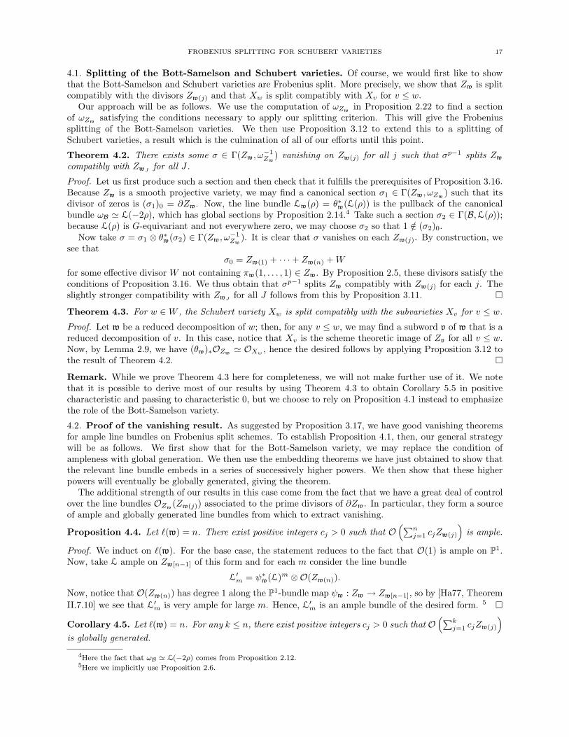
4.1. Splitting of the Bott-Samelson and Schubert varieties. Of course, we would first like to showthat the Bott-Samelson and Schubert varieties are Frobenius split. More precisely, we show that Zw is splitcompatibly with the divisors Zw(j) and that Xw is split compatibly with Xv for v ≤ w.

Our approach will be as follows. We use the computation of ωZw in Proposition 2.22 to find a sectionof ωZw satisfying the conditions necessary to apply our splitting criterion. This will give the Frobeniussplitting of the Bott-Samelson varieties. We then use Proposition 3.12 to extend this to a splitting ofSchubert varieties, a result which is the culmination of all of our efforts until this point.

Theorem 4.2. There exists some σ ∈ Γ(Zw, ω−1Zw

) vanishing on Zw(j) for all j such that σp−1 splits Zw

compatibly with ZwJfor all J .

Proof. Let us first produce such a section and then check that it fulfills the prerequisites of Proposition 3.16.Because Zw is a smooth projective variety, we may find a canonical section σ1 ∈ Γ(Zw, ωZw) such that itsdivisor of zeros is (σ1)0 = ∂Zw. Now, the line bundle Lw(ρ) = θ∗w(L(ρ)) is the pullback of the canonicalbundle ωB ' L(−2ρ), which has global sections by Proposition 2.14.4 Take such a section σ2 ∈ Γ(B,L(ρ));because L(ρ) is G-equivariant and not everywhere zero, we may choose σ2 so that 1 /∈ (σ2)0.

Now take σ = σ1 ⊗ θ∗w(σ2) ∈ Γ(Zw, ω−1Zw

). It is clear that σ vanishes on each Zw(j). By construction, wesee that

σ0 = Zw(1) + · · ·+ Zw(n) +W

for some effective divisor W not containing πw(1, . . . , 1) ∈ Zw. By Proposition 2.5, these divisors satisfy theconditions of Proposition 3.16. We thus obtain that σp−1 splits Zw compatibly with Zw(j) for each j. Theslightly stronger compatibility with ZwJ

for all J follows from this by Proposition 3.11.

Theorem 4.3. For w ∈W , the Schubert variety Xw is split compatibly with the subvarieties Xv for v ≤ w.

Proof. Let w be a reduced decomposition of w; then, for any v ≤ w, we may find a subword v of w that is areduced decomposition of v. In this case, notice that Xv is the scheme theoretic image of Zv for all v ≤ w.Now, by Lemma 2.9, we have (θw)∗OZw ' OXw , hence the desired follows by applying Proposition 3.12 tothe result of Theorem 4.2.

Remark. While we prove Theorem 4.3 here for completeness, we will not make further use of it. We notethat it is possible to derive most of our results by using Theorem 4.3 to obtain Corollary 5.5 in positivecharacteristic and passing to characteristic 0, but we choose to rely on Proposition 4.1 instead to emphasizethe role of the Bott-Samelson variety.

4.2. Proof of the vanishing result. As suggested by Proposition 3.17, we have good vanishing theoremsfor ample line bundles on Frobenius split schemes. To establish Proposition 4.1, then, our general strategywill be as follows. We first show that for the Bott-Samelson variety, we may replace the condition ofampleness with global generation. We then use the embedding theorems we have just obtained to show thatthe relevant line bundle embeds in a series of successively higher powers. We then show that these higherpowers will eventually be globally generated, giving the theorem.

The additional strength of our results in this case come from the fact that we have a great deal of controlover the line bundles OZw(Zw(j)) associated to the prime divisors of ∂Zw. In particular, they form a sourceof ample and globally generated line bundles from which to extract vanishing.

Proposition 4.4. Let `(w) = n. There exist positive integers cj > 0 such that O(∑n

j=1 cjZw(j)

)is ample.

Proof. We induct on `(w). For the base case, the statement reduces to the fact that O(1) is ample on P1.Now, take L ample on Zw[n−1] of this form and for each m consider the line bundle

L′m = ψ∗w(L)m ⊗O(Zw(n)).

Now, notice that O(Zw(n)) has degree 1 along the P1-bundle map ψw : Zw → Zw[n−1], so by [Ha77, TheoremII.7.10] we see that L′m is very ample for large m. Hence, L′m is an ample bundle of the desired form. 5

Corollary 4.5. Let `(w) = n. For any k ≤ n, there exist positive integers cj > 0 such that O(∑k

j=1 cjZw(j)

)is globally generated.

4Here the fact that ωB ' L(−2ρ) comes from Proposition 2.12.5Here we implicitly use Proposition 2.6.

18 YI SUN

Proof. By Proposition 4.4, we may pick cj so thatO(∑k

j=1 cjZw[k](j)

)is ample, henceO

(N∑kj=1 cjZw[k](j)

)is globally generated on Zw[k] for some N . The conclusion follows from Proposition 2.6.

We may now extend the vanishing that we previously had for ample line bundles to globally generatedline bundles and set up a sufficient supply of globally generated line bundles on Zw. Note that the globallygenerated line bundles provided by Lemma 4.7 are designed specifically to prove Proposition 4.1.

Lemma 4.6. Let L be a globally generated line bundle on Zw. Then, we have Hi(Zw,L) = 0 for i > 0.

Proof. Pick cj > 0 so that L′ = O(∑n

j=1 cjZw(j)

)is ample by Proposition 4.4. Let cj =

∑Nl=0 cj,lp

l with0 ≤ cj,l < p be the base p expansion of each cj for some large N that does not depend on j. By Theorem

4.2, we may apply Proposition 3.18 with the bundles O(∑n

j=1 cj,lZw(j)

)for l = N,N − 1, . . . , 0 to obtain

embeddings

Hi(Zw,L) → Hi(Zw,L

p ⊗O( n∑j=1

cj,NZw(j)

))→ Hi

(Zw,L

p2 ⊗O( n∑j=1

(cj,Np+ cj,N−1)Zw(j)

))→ · · · → Hi

(Zw,L

pN+1⊗O

( n∑j=1

cjZw(j)

)).

But now notice that the final line bundle

LpN+1⊗O

( n∑j=1

cjZw(j)

)in the sequence is ample because Lp

N+1is globally generated and O

(∑nj=1 cjZw(j)

)is ample. So by Propo-

sition 3.17, it has vanishing cohomology, hence our embeddings give that Hi(Zw,L) = 0.

Lemma 4.7. Let `(w) = n with w reduced. For any 1 ≤ k, l ≤ n, we may find integers c1, . . . , cn and mwith cj ≥ 0 for 1 ≤ j < k and j > l, cj ≤ 0 for k ≤ j < l, and cl = 0 such that the line bundle

O( n∑j=1

cjZw(j) − Zw(l)

)⊗ Lw(ρ)m

is globally generated.

Proof. We argue by induction on `(w). The base case `(w) = 1 follows from the fact that Lw(ρ) ' O(1)under the identification Zw ' P1. Now suppose `(w) = n and the claim holds for `(w) < n. We now havetwo cases. First, suppose that l < n. In this case, find integers c1, . . . , cn−1,m with cj = 0 for k ≤ j ≤ lsuch that

O( n−1∑j=1

cjZw[n−1](j) − Zw[n−1](l)

)⊗ Lw[n−1](ρ)m

is globally generated. Thus its pullback

ψ∗w

(O( n−1∑j=1

cjZw[n−1](j) − Zw[n−1](l)

)⊗ Lw[n−1](ρ)m

)= O

( n−1∑j=1

cjZw(j) − Zw(l)

)⊗ ψ∗w(Lw[n−1](ρ))m

is globally generated. Now, by Propositions 2.7 and 2.22, we see that

ω−1Zw/Zw[n−1]

⊗ Lw(ρ)h = ω−1Zw⊗ ψ∗w(ωZw[n−1])⊗ Lw(ρ)h

= O(∂Zw)⊗ Lw(ρ)h+1 ⊗O(−n−1∑j=1

Zw(j)

)⊗ ψ∗wLw[n−1](−ρ)

= O(Zw[n−1])⊗ Lw(ρ)h+1 ⊗ ψ∗wLw[n−1](−ρ)


is the pullback of ω−1B/(G/Pin ) ⊗ L(ρ)h = L(αin + hρ). Thus, we see that, for large h, αin + hρ is dominant,

hence the line bundle is globally generated by Corollary 2.18. Tensoring together the two line bundles wehave shown to be globally generated, we see that

O( n−1∑j=1

cjZw(j) − Zw(l)

)⊗O(mZw(n))⊗ Lw(ρ)m(h+1)

is globally generated, as needed.Now consider the case l = n. In this case, consider the line bundle Lw(χin) on Zw for χin the fundamental

weight corresponding to sin . By Lemma 2.21, χin has degree 1 along the fibers of ψw, hence by Proposition2.23 we have in Pic(Zw) the identity

Lw(χin) = O(Zw(n)) +O( n−1∑j=1

djZw(j)

)for some dj . We claim that dj ≥ 0 for all j. For this, we will need to use the fact that w is a reduced word. By

Corollary 2.18, we see that Lw(χin) is globally generated, hence O(Zw(n) +

∑n−1j=1 djZw(j)

)is an effective

divisor. Now, because Lw(χin) is B-equivariant, we may find a global section σ ∈ Γ(Zw,Lw(χin) which isB-invariant up to scaling. Such a σ has a B-invariant zero divisor σ0, and in addition Lw(χin) = OZw(σ0).Now, because w is reduced, Zw− ∂Zw → Cw is an isomorphism by Proposition 2.8, hence it is a dense orbitof the B-action on Zw. This shows that σ0 ⊂ ∂Zw, so we obtain that Lw = O(σ0) is in the non-negativespan of O(Zw(j)), as needed.

Now, by Corollary 2.18, we see that

Lw(ρ− χin) = Lw(ρ)⊗O(−Zw(n))⊗O(−n−1∑j=1

djZw(j)

)is globally generated. By Corollary 4.5, we may find c′1, . . . , c

′k−1 large and positive such thatO

(∑k−1j=1 c

′jZw(j)

)is globally generated. Tensoring these two line bundles, we obtain that

Lw(ρ)⊗O(−Zw(n))⊗O( k−1∑j=1

c′jZw(j) −n−1∑j=1

djZw(j)

)is globally generated, as needed.

We are now ready to prove Proposition 4.1. Our strategy will be to embed the desired cohomology intothe cohomology of a line bundle which is the product of a line bundles of the form given in Lemma 4.7 andother globally generated line bundles. The conclusion will then follow from Lemma 4.6.

Proof of Proposition 4.1. First, if λ is dominant, Lw(λ) is globally generated as the pullback of the globallygenerated line bundle L(λ) by Lemma 2.14. The second assertion then follows from Lemma 4.6. For therest of the proof, replace Lw(λ) by any globally generated line bundle L on Zw.

We will emulate the proof of Proposition 4.6. However, our sequence of embeddings will be a bit moredelicate here. First, let us use Lemma 4.7 to construct a special globally generated line bundle. For k ≤ t ≤ l,we may find globally generated line bundles Lt = O

(∑nj=1 c

′j,tZw(j) − Zw(t)

)⊗ Lw(ρ)mj with cj,t ≥ 0 for

1 ≤ j < k and j > t, cj,t ≤ 0 for k ≤ j < t, and ct,t = 0. Therefore, we may inductively construct a globallygenerated line bundle of the form

L′ = Lak

k ⊗ · · · ⊗ Lal

l = O( n∑j=1

djZw(j)

)⊗ Lw(ρ)m

for some positive integers ak, . . . , al such that dj < 0 for k ≤ j ≤ t and dj ≥ 0 otherwise.

We now embed Hi(Zw,L

h ⊗O(−∑lj=k Zw(j)

))into Hi(Zw,L

′). We may rewrite the form of L′ as

L′ = O( k−1∑j=1

djZw(j) +n∑

j=l+1

djZw(j) −l∑

j=k

ejZw(j)

)⊗ Lw(ρ)m

20 YI SUN

for ej = −dj > 0. Fix some N such that pN+1 > maxjdj , ej, and take base p expansions dj =∑Nr=0 dj,rp

r,m =

∑Nr=0mrp

r, and pN+1−ej =∑Nr=0 ej,rp

r, for some 0 ≤ dj,r,mr, ej,r < p. We will now apply Proposition3.18 a total of N + 1 times, where at step N + 1− r, we will apply it to multiply by the bundle

O( ∑j /∈[k,l]

dj,rZw(j) +l∑

j=k

ej,rZw(j)

)⊗ Lw(ρ)mr .

This gives rise to the sequence of embeddings

Hi(Zw,L

h ⊗O(−

l∑j=k

Zw(j)

))

→ Hi(Zw,L

hp ⊗O( ∑j /∈[k,l]

dj,NZw(j) +l∑

j=k

(ej,N − p)Zw(j)

)⊗ Lw(ρ)mN

)

→ Hi(Zw,L

hp2 ⊗O( ∑j /∈[k,l]

(dj,N−1 + dj,Np)Zw(j) +l∑

j=k

(ej,N−1 + ej,Np− p2)Zw(j)

)⊗ Lw(ρ)mN−1+mNp

)→ · · ·

→ Hi(Zw,L

hpN+1⊗O

( ∑j /∈[k,l]

( N∑r=0

dj,rpr)Zw(j) +

l∑j=k

(− pN+1 +

N∑r=0

ej,rpr)Zw(j)

)⊗ Lw(ρ)

∑Nr=0mrp

r)

= Hi(Zw,LhpN+1

⊗ L′).

But recall that L′ was constructed to be globally generated, hence LhpN+1 ⊗L′ is globally generated. There-

fore, by Proposition 4.6, the final cohomology vanishes, so all the cohomologies in the chain of embeddingsvanish, as needed.

4.3. Passing to characteristic 0. We now transfer Proposition 4.1 to the characteristic 0 case. Let usnow consider all schemes to be over Spec(Z) instead of Spec(k) (as we were implicitly assuming before). Wewould like to apply the semi-continuity theorem, stated below.

Theorem 4.8 ([Ha77, Theorem 12.8]). Let X → Y be a projective morphism of Noetherian schemes, andlet F be a coherent sheaf on X, flat over Y . Then, for each i ≥ 0, the function

hi(y,F) = dimk(y)Hi(Xy,Fy)

is an upper semicontinuous function on Y .

For this, we need coherent sheaves, flat over some base. In this case, they will be provided by genericflatness.

Lemma 4.9 ([Eis, Theorem 14.4]). If F is a coherent sheaf on a scheme X defined over Z, then there is afinite set S of primes such that the sheaf FZ[S−1] given by base change from Z to Z[S−1] is flat over Z[S−1].

We may apply semi-continuity and Lemma 4.9 to obtain the following.

Proposition 4.10. Let X be a projective scheme over Z. Let F be a coherent sheaf on X, and let i ≥ 0. IfHi(Xp,Fp) = 0 for any p, then Hi(XQ,FQ) = 0.

Proof. By Lemma 4.9, we may find some finite set of primes S such that FZ[S−1] is flat over Z[S−1]. So inparticular, we may take S = Spec(Z)− (0), (p) for some prime p.

Now, suppose otherwise for contradiction. By [Ha77, Proposition 9.3], we have that

Hi(XQ,FQ) = Hi(XQ,FQ)⊗Q

Q,

meaning that hi((0),F) > 0. Now, the set x | hi((x),F) is closed in Spec(Z[S−1]), but the closure of (0)contains all of Spec(Z[S−1]), which implies that hi((p),F) > 0. Again applying [Ha77, Proposition 9.3], wehave that

Hi(Xp,Fp) = Hi(Xp,Fp) ⊗Fp

Fp,


meaning that hi((p),F) = 0, a contradiction. So we must have Hi(XQ,FQ) = 0.

The relevant sheaves in Proposition 4.1 are line bundles over Zw, hence coherent. Furthermore, Zw isprojective, so Proposition 4.10 implies that the result holds for Q. Finally, for any other algebraically closedfield k of characteristic 0, we may again use [Ha77, Proposition 9.3] to obtain that

Hi((Zw)k,Fk) = Hi((Zw)Q,FQ) ⊗Qk = 0

for any coherent sheaf F on Zw. Hence Proposition 4.1 remains valid in characteristic 0.

5. Proofs of the main results

Having condensed the technical input of Frobenius splitting into Proposition 4.1, let us recall our originalpurpose. We began with the construction of the flag variety B and Schubert varieties Xw ⊂ B. To understandthe geometry of Xw, we constructed their desingularizations Zw → Xw via the Bott-Samelson varieties.Armed with our newly developed cohomology vanishing result on Zw, we will now retrace our steps and useit to show that the geometry of Xw is remarkably nice.

We will show that the Schubert varieties Xw are normal, Cohen-Macaulay, and have rational resolutions.Further, line bundles Lw(λ) on them will satisfy a certain character formula known as the Demazure characterformula, which we view as a refinement of the usual Weyl character formula. Our results in this section willhold over arbitrary characteristic, as the only result we will draw from our Frobenius splitting methods isProposition 4.1.

5.1. Schubert varieties are normal and Cohen-Macaulay. In this subsection, we first draw someadditional technical consequences of Proposition 4.1. We would like to emphasize that these are more or lessformal consequences and do not require significant geometric insight to prove.

Corollary 5.1. For any w, 1 ≤ j ≤ n and dominant weight λ, the map

H0(Zw,Lw(λ))→ H0(Zw(j),Lw(j)(λ))

induced by the inclusion ιw,j : Zw(j) → Zw is surjective.

Proof. Viewing Zw(j) as a closed subvariety in Zw, we have the exact sequence

0→ OZw(−Zw(j))→ OZw → (ιw,j)∗OZw(j) → 0.

Now, we may tensor with the line bundle Lw(λ) to obtain

0→ Lw(λ)⊗OZw(−Zw(j))→ Lw(λ)→ (ιw,j)∗Lw(j)(λ)→ 0,

where we note that ι∗w,jLw(λ) = Lw(j)(λ). The result follows upon applying the long exact sequence incohomology and obtaining that H1(Zw,Lw(λ)⊗OZw(−Zw(j))) = 0 from Proposition 4.1.

We now introduce a lemma from homological algebra in order to obtain the next consequence, Corollary5.3, which will be the form in which we would like to view our technical input.

Lemma 5.2. Let F be a line bundle on Zw such that for any i > 0 and m large, we have Hi(Zw,F ⊗Lw(ρ)m) = 0. We have Ri(θw)∗F = 0 for i > 0.

Proof. Note that ρ is dominant, hence Lw(ρ) is ample on Xw. For any m, we have the Leray spectralsequence associated to θw : Zw → Xw given by

Hj(Xw, Ri(θw)∗(F ⊗ Lw(λ)m)) =⇒ Hj+i(Zw,F ⊗ (θw)∗Lw(λ)m).

Now, for j > 0, we have

Hj(Xw, Ri(θw)∗(F ⊗ Lw(λ)m)) ' Hj(Xw, R

i(θw)∗F ⊗ Lw(λ)m) = 0

for m large because Lw(λ) is ample. For such an m, the spectral sequence degenerates and we have

H0(Xw, Ri(θw)∗F ⊗ Lw(λ)m) ' Hi(Zw,F ⊗ Lw(λ)m) = 0

for any i > 0 by our assumption on F. But for large m, Ri(θw)∗F ⊗ Lw(λ)m is globally generated becauseLw(λ) is ample, hence Ri(θw)∗F = 0.

Corollary 5.3. Let w be a reduced word with p(w) = w. We have the following:

22 YI SUN

(i) For any i > 0, we have that Ri(θw)∗OZw = Ri(θw)∗ωZw = 0;(ii) θw induces an isomorphism of line bundles (θw)∗OZw ' OXw ;

(iii) For any locally free sheaf F on Xw, we have Hi(Xw,F) ' Hi(Zw, (θw)∗F) for i ≥ 0.

Proof. For (i), note that OZw and ωZw satisfy the conditions of Lemma 5.2 by Proposition 4.1. 6 Statement(ii) is exactly Lemma 2.9; we state it here for completeness only. For (iii), the Leray spectral sequence

Hj(Xw, Ri(θw)∗OZw ⊗ F) =⇒ Hi+j(Zw, (θw)∗F)

degenerates by (i), hence in the j = 0 case we obtain Hi(Xw,F) = Hi(Zw, (θw)∗F).

Results (i) and (ii) of Corollary 5.3 together make up the fact that θw : Zw → Xw is a rational resolution.Using these formal properties, we may now prove the following, our first main result.

Theorem 5.4. For any w ∈W , the Schubert variety Xw is normal and Cohen-Macaulay.

Proof. We first show that Xw is normal. This follows immediately from Corollary 5.3(ii) because θw is abirational map to Xw from the smooth variety Zw.

We now show that Xw is Cohen-Macaulay. Because Xw is projective of dimension n = `(w), it suffices by[Ha77, Theorem 7.6] to show that for any ample line bundle L on Xw, we have Hi(Xw,L

−m) = 0 for i < nand m sufficiently large. 7 We now have

Hi(Xw,L−m) ' Hi(Zw, (θw)∗L−m) ' Hn−i(Zw, ωZw ⊗ (θw)∗Lm) ' Hn−i(Xw, (θw)∗(ωZw)⊗ Lm) = 0

for m large because L is ample. Here, the first isomorphism is by Corollary 5.3(iii), the second by Serreduality on the smooth projective variety Zw, and the last by the Leray spectral sequence and the projectionformula.

5.2. Demazure character formula. We now come to our original motivation for studying the geometryof Schubert varieties. Recall that the Borel-Weil theorem related the irreducible representations of G to theglobal sections of the line bundles L(λ) on B. We would like to obtain an analogue of this result for Lw(λ).Notice, however, that Xw has only an action of B and not of G, so the cohomologies Hi(Xw,Lw(λ)) areonly B-modules, not G-modules. Thus, we can at most hope for a character formula for these modules, and,indeed, one exists. First, however, we note that in fact we do not need to consider the higher cohomologies.

Corollary 5.5. For any Schubert variety Xw and any dominant weight λ, we have that Hi(Xw,Lw(λ)) = 0for i > 0 and the restriction map H0(B,L(λ))→ H0(Xw,Lw(λ)) is surjective.

Proof. This follows immediately from Corollaries 5.1 and 5.3(iii).

We are now ready to state the Demazure character formula. Recall that any finite dimensional T -moduleM splits uniquely as the sum of its weight spaces Mλ for λ ∈ X∗(T ). Then, we may define the characterchM of M as the formal sum

chM =∑

λ∈X∗(T )

dimMλ eλ,

where we interpret chM in Z[X∗(T )]. Now, for any simple reflection si ∈W , define the Demazure operatorDsi

: Z[X∗(T )]→ Z[X∗(T )] associated to si by

Dsi(eλ) =

eλ − esiλ−αi

1− e−αi.

It is easy to check that Dsi is a linear operator Z[X∗(T )]→ Z[X∗(T )] and is given explicitly by

(2) Dsi(eλ) =

eλ + eλ−αi + · · ·+ esiλ if 〈λ, α∨i 〉 ≥ 00 if 〈λ, α∨i 〉 = −1−(eλ+αi + · · ·+ esiλ−αi) if 〈λ, α∨i 〉 < −1.

For any word w = (si1 , . . . , sin), we write Dw = Dsi1 · · · Dsin

. We now have the character formula.

6Here we use implicitly that ωZw ⊗ Lw(ρ)2 = O(−∂Zw)⊗ Lw(ρ) by Proposition 2.22.7Applying [Ha77, Theorem 7.6] as stated requires that Hi(Xw,F ⊗ L−m) = 0 for i < n and m sufficiently large for all

locally free sheaves F. From the proof in [Ha77], however, only the case F = OXw is used.


Theorem 5.6 (Demazure character formula). Let w be any reduced decomposition of w and λ a dominantweight. Then, we have that

ch Γ(Xw,Lw(λ)) = Dw(eλ),

where eλ = e−λ is an involution on Z[X∗(T )].

Proof. We will write Dw instead of Dw. By Corollary 5.3 and Proposition 5.5, it suffices to show thatχ(Zw,Lw(λ)) = Dw(eλ), where χ(Zw,Lw(λ)) denotes the characteristic

χ(Zw,Lw(λ)) =∑i

(−1)i chHi(Zw,Lw(λ)).

We will instead show the stronger statement that χ(Zw,Lw(M)) = Dw(chM) for any T -module M . Thisstatement will follow directly from the geometry of Zw, requiring no input from our Frobenius splittingmethods. The desired is then the case M = k−λ.

First, for any short exact sequence

0→M1 →M2 →M3 → 0

of T -modules, we have Dw(chM2) = Dw(chM1) + Dw(chM3) by the definition of ch. Further, by Lemma2.17, the functor Lw(−) is exact, meaning that the functor χ(Zw,Lw(−)) is exact, so we have χ(Zw,Lw(M2)) =χ(Zw,Lw(M1)) + χ(Zw,Lw(M3)). Thus, because any T -module is completely reducible, for a fixed `(w) itis enough for us to show that χ(Zw,Lw(λ)) =

∑i(−1)i chHi(Zw,Lw(λ)) for all λ.

We now proceed by induction on `(w). 8 For `(w) = 0, we have w = 1. Hence, we see that

Γ(X1,Lw(λ)) = L(λ)1 = (G×B k−λ)1 ' k−λ,as needed. Now, for `(w) = 1, we find that

χ(Psi/B,Lsi

(λ)) = Dsi(e−λ)

using Lemma 2.20, Serre duality on P1, and the explicit form of Dsi(eλ) given in Equation (2).

In the general case, for `(w) = n, consider the map ψw : Zw → Zw[n−1], which gives the Leray spectralsequence

Ei,j2 = Hi(Zw[n−1], Rj(ψw)∗Lw(λ)) =⇒ Hi+j(Zw,Lw(λ)).

Now, we claim that

(3) Rj(ψw)∗Lw(λ) ' Lw[n−1](Hj(Pin/B,Lsin(λ))) = Lw[n−1](Hj(Zsin

,Lsin(λ))).

The proof of this will be extremely technical, so we postpone it in favor of the conclusion of our argument.Because the spectral sequence converges, we have

χ(Zw,Lw(λ)) =∑j

(−1)jχ(Zw[n−1],Lw[n−1](Hj(Zsin,Lsin

(λ))))

=∑j

(−1)jDw[n−1](chHj(Zsin,Lsin

(λ)))

= Dw[n−1](χ(Zsin,Lsin

(λ)))

= Dw[n−1](Dsin(e−λ))

= Dw(e−λ))

using the inductive step for Zw[n−1] and Zsin. This completes the induction.

We now prove (3) modulo one technical claim for which we will appeal to [Jan]. We first claim that itsuffices to give an isomorphism of functors 9

(4) (ψw)∗Lw(−) ' Lw[n−1](Γ(Zsin,Lsin

(−))).

Indeed, it would then suffice to show that Rj(ψw)∗LZw vanishes on injective T -modules, as the desired claimwould follow by taking the jth right derived functor of both sides and noting that Lw(−), Lw[n−1](−), andLsin

(−) are exact by Lemma 2.17. This fact is checked in [Jan, II.5.19].

8It is important to note that our induction is still for general M .9Here, we are using Lemma 2.16 to interpret the functors Lw, Lw[n−1], and Lsin

.

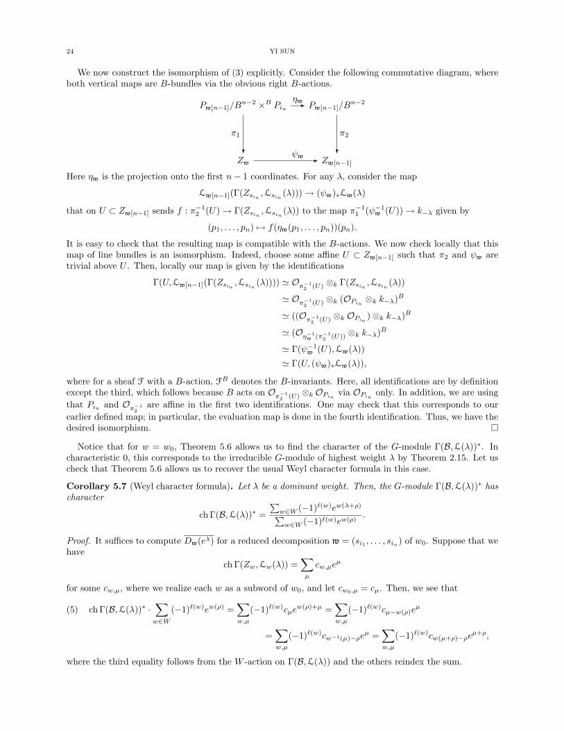
24 YI SUN

We now construct the isomorphism of (3) explicitly. Consider the following commutative diagram, whereboth vertical maps are B-bundles via the obvious right B-actions.

Pw[n−1]/Bn−2 ×B Pin

ηw- Pw[n−1]/Bn−2

Zw

π1

? ψw - Zw[n−1]

π2

?

Here ηw is the projection onto the first n− 1 coordinates. For any λ, consider the map

Lw[n−1](Γ(Zsin,Lsin

(λ)))→ (ψw)∗Lw(λ)

that on U ⊂ Zw[n−1] sends f : π−12 (U)→ Γ(Zsin

,Lsin(λ)) to the map π−1

1 (ψ−1w (U))→ k−λ given by

(p1, . . . , pn) 7→ f(ηw(p1, . . . , pn))(pn).

It is easy to check that the resulting map is compatible with the B-actions. We now check locally that thismap of line bundles is an isomorphism. Indeed, choose some affine U ⊂ Zw[n−1] such that π2 and ψw aretrivial above U . Then, locally our map is given by the identifications

Γ(U,Lw[n−1](Γ(Zsin,Lsin

(λ)))) ' Oπ−12 (U) ⊗k Γ(Zsin

,Lsin(λ))

' Oπ−12 (U) ⊗k (OPin

⊗k k−λ)B

' ((Oπ−12 (U) ⊗k OPin

)⊗k k−λ)B

' (Oη−1w (π−1

2 (U)) ⊗k k−λ)B

' Γ(ψ−1w (U),Lw(λ))

' Γ(U, (ψw)∗Lw(λ)),

where for a sheaf F with a B-action, FB denotes the B-invariants. Here, all identifications are by definitionexcept the third, which follows because B acts on Oπ−1

2 (U) ⊗k OPinvia OPin

only. In addition, we are usingthat Pin and Oπ−1

2are affine in the first two identifications. One may check that this corresponds to our

earlier defined map; in particular, the evaluation map is done in the fourth identification. Thus, we have thedesired isomorphism.

Notice that for w = w0, Theorem 5.6 allows us to find the character of the G-module Γ(B,L(λ))∗. Incharacteristic 0, this corresponds to the irreducible G-module of highest weight λ by Theorem 2.15. Let uscheck that Theorem 5.6 allows us to recover the usual Weyl character formula in this case.

Corollary 5.7 (Weyl character formula). Let λ be a dominant weight. Then, the G-module Γ(B,L(λ))∗ hascharacter

ch Γ(B,L(λ))∗ =∑w∈W (−1)`(w)ew(λ+ρ)∑w∈W (−1)`(w)ew(ρ)

.

Proof. It suffices to compute Dw(eλ) for a reduced decomposition w = (si1 , . . . , sin) of w0. Suppose that wehave

ch Γ(Zw,Lw(λ)) =∑µ

cw,µeµ

for some cw,µ, where we realize each w as a subword of w0, and let cw0,µ = cµ. Then, we see that

(5) ch Γ(B,L(λ))∗ ·∑w∈W

(−1)`(w)ew(ρ) =∑w,µ

(−1)`(w)cµew(ρ)+µ =

∑w,µ

(−1)`(w)cµ−w(ρ)eµ

=∑w,µ

(−1)`(w)cw−1(µ)−ρeµ =

∑w,µ

(−1)`(w)cw(µ+ρ)−ρeµ+ρ,

where the third equality follows from the W -action on Γ(B,L(λ)) and the others reindex the sum.


We now claim that

(6)∑w

(−1)`(w)cv,w(µ+ρ)−ρ =

(−1)`(w) µ = w(λ+ ρ)− ρ for some w ∈W0 otherwise

for all v ∈W . Let us first show how this implies the desired and defer the proof until afterward. Specializingto v = w0 and substituting into Equation (5), we see that

ch Γ(B,L(λ))∗ ·∑w∈W

(−1)`(w)ew(ρ) =∑µ

eµ+ρ∑w

(−1)`(w)cw(µ+ρ)−ρ =∑w

(−1)`(w)ew(λ+ρ),

which gives the desired character formula.It suffices now to establish (6). We argue by induction on `(v). For the base case `(v) = 0, the conclusion

is clear. Now, write v = siu with `(u) = `(v)− 1 and notice that∑µ

cv,µeµ = Dsi

(∑µ

cu,µeµ)

=∑µ

cu,µ

(eµ∞∑k=0

e−kαi − esiµ∞∑k=1

e−kαi

),

where we take Dsi instead of Dsibecause we are taking the dual of Γ(B,L(λ))∗. Taking the coefficients of

eµ on both sides, we obtain

cv,µ =∞∑k=0

cu,µ+kαi −∞∑k=1

cu,siµ−kαi .

Substituting into the desired sum, we obtain∑w

(−1)`(w)cv,w(µ+ρ)−ρ =∑w

(−1)`(w)∞∑k=0

cu,w(µ+ρ)+kαi−ρ −∑w

(−1)`(w)∞∑k=1

cu,siw(µ+ρ)−kαi−siρ

=∑w

(−1)`(w)∞∑k=0

cu,w(µ+ρ)+kαi−ρ +∑w

(−1)`(w)∞∑k=1

cu,w(µ+ρ)−(k−1)αi−ρ

=∑w

∞∑k=−∞

(−1)`(w)cu,w(µ+ρ)+kαi−ρ +∑w

(−1)`(w)cu,w(µ+ρ)−ρ,

where the second equality follows by reindexing the summation over siw and noting that siρ = ρ− αi. Bya similar reindexing, we see that∑

w

∞∑k=−∞

(−1)`(w)cu,w(µ+ρ)+kαi−ρ = −∑w

∞∑k=−∞

(−1)`(w)cu,siw(µ+ρ)+kαi−ρ

= −∑w

∞∑k=−∞

(−1)`(w)cu,w(µ+ρ)+(k−〈α∨i ,w(µ+ρ)〉αi−ρ

= −∑w

∞∑k=−∞

(−1)`(w)cu,w(µ+ρ)+kαi−ρ,

which means that∑w

∑∞k=−∞(−1)`(w)cu,w(µ+ρ)+kαi−ρ = 0. So we may conclude that∑

w

(−1)`(w)cv,w(µ+ρ)−ρ =∑w

(−1)`(w)cu,w(µ+ρ)−ρ =

(−1)`(w) µ = w(λ+ ρ)− ρ for some w ∈W0 otherwise,

completing the induction.

Remark. In the proof of Corollary 5.7, the expression w(µ+ ρ)− ρ occurs several times. This is known asthe dotted action of W on X∗(T ).

26 YI SUN

Appendix A. Duality for the Frobenius morphism on smooth varieties

In this appendix we provide the technical details necessary to provide an explicit version of finite flatduality for the Frobenius morphism F : X → X on a smooth variety. Our model will be Theorem A.1 below,which gives the more general duality that holds in this situation.

Theorem A.1 ([Ha66, III.6-10]). Let X,Y be Noetherian schemes and f : X → Y a finite flat morphismwith fibers of dimension 0. Then, there exists a pair (ωf ,Trf ) of a line bundle ωf on X and a map Trf :f∗ωf → OY given by evaluation at 1 such that for any F ∈ QCoh(X), the bilinear pairing

f∗HomOX(F, ωf )× f∗F → f∗ωf

Trf→ OYinduces an isomorphism

f∗HomOX(F, ωf ) ' HomOY

(f∗F,OY ).In this situation, we may take ωf = HomOY

(f∗OX ,OY ) ' ωX/Y .

While it is in theory possible to extract the trace map Trf : f∗ωf → OY from the general nonsenseused in the proof of Theorem A.1, in practice this is extremely involved. In our case, we know that themorphism is in fact the Frobenius map F : X → X on a smooth variety X, allowing us to provide analternate description of this duality in Proposition 3.14. Note that the trace map of Theorem A.1 becomesthe composition F∗ω

1−pX → HomOX

(F∗OX ,OX)→ OX in this new formulation.Our strategy will be as follows. We first explicitly construct a map C : F∗ωX → ωX with a nice form in

local coordinates. We then use C to construct a map F∗ω1−pX → HomOX

(F∗OX ,OX), which we show is anisomorphism by looking at its local properties. Let us begin by constructing this map.

Proposition A.2. Let X be a smooth variety. There is a map C : F∗ωX → ωX of OX-modules whose localexpansion takes the form

C(ta · ω) = δp(a + 1)ta+1

p −1 · ω.

Proof. Let us first construct a map f : ωX → F∗(ωX/dΩn−1X ). We claim that there is a map on affines

fA : Ω1A → F∗(Ω1

A/dΩ0A) given by adb 7→ apbp−1db. We first check that fA is a valid map. Indeed, we find

directly thatfA(adb) = apfA(db) = a · fA(db)

andfA(d(ab)) = ap−1bp−1d(ab) = apbp−1db+ ap−1bpda = fA(adb+ bda).

For the final verification, notice that

p(a+ b)p−1d(a+ b) = d((a+ b)p) =p∑i=0

(p

i

)d(aibp−i) = pap−1da+ pbp−1db+

p−1∑i=1

(p

i

)d(aibp−i)

as integer polynomials. Therefore, dividing by p, we see that

fA(d(a+ b))− fA(da)− fA(db) = (a+ b)p−1d(a+ b)− ap−1da− bp−1db =p−1∑i=1

1p

(p

i

)d(aibp−i) ∈ Im(Ω0

A)

because p |(pi

)for 1 ≤ i ≤ p− 1. So we see that fA gives a valid map Ω1

A → F∗(Ω1A/Ω

0A).

Taking this map on each affine and applying the nth exterior power, we obtain a map f : ωX →F∗(ωX/Ωn−1

X ). Locally, f is given on each Spec(A) by

adb1 ∧ · · · ∧ dbn 7→ apbp−11 · · · bp−1

n db1 ∧ · · · ∧ dbn.We now claim that f is an isomorphism. It suffices to check this in local coordinates t1, . . . , tn at all pointsx ∈ X. In this case, the map becomes

g(t1, . . . , tn) · ω 7→ g(t1, . . . , tn)ptp−11 · · · tp−1

n · ω.

Let us first examine the space dΩn−1k[[t1,...,tn]]. Notice that for a with δp(a + 1) = 0, we have

ta · ω = ∂ti

(1

ai + 1ta11 · · · t

ai−1i−1 t

ai+1i t

ai+1i+1 · · · t

ann dt1 ∧ · · · ∧ dti−1 ∧ dti+1 · · · ∧ dtn

)∈ dΩn−1

k[[t1,...,tn]],


where i is chosen so that ai + 1 6≡ 0 (mod p). On the other hand, if δp(a + 1) = 1, we see that ∂ti(ta · dt1 ∧

· · · ∧ dti ∧ · ∧ dtn) = 0 for all i, hence dΩn−1k[[t1,...,tn]] is spanned over k[[t1, . . . , tn]] by monomials ta · ω with

δp(a + 1) = 0. But notice that the action is twisted by the Frobenius map F : k[[t1, . . . , tn]]→ k[[t1, . . . , tn]],meaning that the action of k[[t1, . . . , tn]] on a monomial produces only monomials with exponents of thesame residue modulo p. Thus we conclude that dΩn−1

k[[t1,...,tn]] consists of formal power series containing onlymonomials of the form ta, where δp(a + 1) = 0.

Deducing that f is an isomorphism is now straightforward. Any g(t1, . . . , tn)·ω ∈ Ωnk[[t1,...,tn]]/dΩn−1k[[t1,...,tn]]

is equal to the sum of its monomials cata with δp(a + 1) = 1. But these are evidently in the image of f ,hence f is surjective. Now, suppose that f kills some

∑a cat

a. This means that

f(∑

a

cata)

=∑a

cpatpa+p−1 ∈ dΩn−1

k[[t1,...,tn]],

which is impossible, since elements dΩn−1k[[t1,...,tn]] contain no monomials of the form tpa+p−1. Hence f is also

injective, completing the proof that f is an isomorphism.

Now, we claim that C : F∗ωX → F∗(ωX/dΩn−1X )

f−1

→ ωX is the desired map. Notice that C(ta · ω) =g(t1, . . . , tn) · ω satisfies

f(g(t1, . . . , tn) · ω)− ta · ω = g(t1, . . . , tn)ptp−1 · ω − ta · ω ∈ dΩn−1k[[t1,...,tn]]

and that C(ta · ω) is uniquely defined by this. Thus we see immediately that when δp(a + 1) = 1, we haveC(ta ·ω) = t

a+1p −1. On the other hand, for δp(a + 1) = 0, we showed above that ta ·ω ∈ dΩn−1

k[[t1,...,tn]], hencewe have that C(ta · ω) = 0 in this case. So C has the desired local form.

Now that we know the local behavior of the map C, we may use it to construct the desired isomorphism.In particular, this will allow us to check for isomorphism locally.

Proof of Proposition 3.14. We first define the map abstractly and then check that it is an isomorphism fromits local description. Consider the composition of identifications

F∗ω1−pX → F∗(ω

−pX ⊗ ωX)→ ω−1

X ⊗ F∗ωX → HomOX(F∗OX ,OX),

where the first is clear, the second results from the identification ω−1X ⊗ F∗OX ' F ∗ω−1

X ' ω−pX given byw ⊗ f 7→ wpf and the projection formula, and the last by tensoring ω−1

X with

F∗OX ⊗ F∗ωXmult→ F∗ωX

C→ ωX .

Now, tracing the map in local coordinates t1, . . . , tn at some x ∈ X, it maps

ta · ω1−p 7→ ω−p ⊗ ta · ω 7→ ω−1 ⊗ ta · ω 7→(tb 7→ C(ta+b · ω) · ω−1

)=(tb 7→ δp(a + b + 1)t

a+b+1p −1

),

where we’ve used the local expansion of C. Finally, to check that the map is an isomorphism, we may againcheck at each point x ∈ X in local coordinates. But in this case, we have an explicit inverse

Homk[[t1,...,tn]](F∗k[[t1, . . . , tn]], k[[t1, . . . , tn]])→ F∗k[[t1, . . . , tn]]

given byf 7→

∑a<p−1

f(ta)p,

where by a < p− 1 we mean that 0 ≤ ai < p. Verifying that these maps are inverse is straightforward afternoting that a map F∗k[[t1, . . . , tn]]→ k[[t1, . . . , tn]] is specified uniquely by its values on ta for a < p−1.

28 YI SUN

References

[And] H. H. Andersen, Schubert varieties and Demazure’s character formula, Invent. Math. 79 (1985), 611-618.

[BK] M. Brion and S. Kumar, Frobenius Splitting Methods in Geometry and Representation Theory, Birkhauser, Progress inMathematics 231, 2005.

[Dem] M. Demazure, Desingularisation des varietes de Schubert generalisees, Ann. Sci. Ecole Norm. Sup. 7 (1974), 53-85.[Eis] D. Eisenbud, Commutative Algebra with a View Toward Algebraic Geometry, Springer, Graduate Texts in Mathematics

150, 1995.

[FI] R. Fossum and B. Iversen, On Picard groups of algebraic fibre spaces, J. Pure Appl. Algebra 3 (1973), 269-289.[Ha66] R. Hartshorne, Residues and Duality, Springer, Lecture Notes in Mathematics 20, 1966.

[Ha77] , Algebraic Geometry, Springer, Graduate Texts in Mathematics 52, 1977.[Jan] J. C. Jantzen, Representations of Algebraic Groups, Academic Press, Pure and Applied Mathematics 131, 1987.

[Kem] G. R. Kempf, Linear systems on homogeneous spaces, Ann. of Math. 103 (1976), 557-591.

[Kum] S. Kumar, Demazure character formula in arbitrary Kac-Moody setting, Invent. Math. 89 (1987), 395-423.[LT] N. Lauritzen and J. F. Thomsen, Line bundles on Bott-Samelson varieties, J. Algebraic Geom. 13 (2004), 461-473.

[MS] V. B. Mehta and V. Srinivas, Normality of Schubert Varieties, Amer. J. Math. 109 (1987), 987-989.

[MR] V. B. Mehta and A. Ramanathan, Frobenius splitting and cohomology vanishing for Schubert varieties, Ann. of Math.122 (1985), 27-40.

[Ram] A. Ramanathan, Schubert varieties are arithmetically Cohen-Macaulay, Invent. Math. 85 (1985), 283-294.

[Spr] T. Springer, Linear Algebraic Groups, Birkhauser, Progress in Mathematics 9, 2008.

206 Cabot Mail Center, Cambridge, MA 02138E-mail address: [email protected]

frobenius splitting for schubert …yisun.io/notes/frobsplit.pdffrobenius splitting for schubert...

Documents