9 early stopping of clinical trials - nc state university 9 st 520, a. tsiatis 9 early stopping of...

CHAPTER 9 ST 520, A. TSIATIS

9 Early Stopping of Clinical Trials

9.1 General issues in monitoring clinical trials

Up to now we have considered the design and analysis of clinical trials assuming the data would

be analyzed at only one point in time; i.e. the final analysis. However, due to ethical as well

as practical considerations, the data are monitored periodically during the course of the study

and for a variety of reasons may be stopped early. In this section we will discuss some of the

statistical issues in the design and analysis of clinical trials which allow the possibility of early

stopping. These methods fall under the general title of group-sequential methods.

Some reasons a clinical trial may be stopped early include

• Serious toxicity or adverse events

• Established benefit

• No trend of interest

• Design or logistical difficulties too serious to fix

Since there is lot invested (scientifically, emotionally, financially, etc.) in a clinical trial by

the investigators who designed or are conducting the trial, they may not be the best suited

for deciding whether the clinical trial should be stopped. It has become common practice for

most large scale phase III clinical trials to be monitored by an independent data monitoring

committee; often referred to as a Data Safety Monitoring Board (DSMB). It is the responsibility

of this board to monitor the data from a study periodically (usually two to three times a year)

and make recommendations on whether the study should be modified or stopped. The primary

responsibility of this board is to ensure the safety and well being of the patients that have enrolled

into the trial.

PAGE 141


The DSMB generally has members who represent the following disciplines:

• Clinical

• Laboratory

• Epidemiology

• Biostatistics

• Data Management

• Ethics

The members of the DSMB should have no conflict of interest with the study or studies they

are monitoring; e.g. no financial holdings in the company that is developing the treatments by

member or family. All the discussions of the DSMB are confidential. The charge of the DSMB

includes:

• Protocol review

• Interim reviews

– study progress

– quality of data

– safety

– efficacy and benefit

• Manuscript review

During the early stages of a clinical trial the focus is on administrative issues regarding the

conduct of the study. These include:

• Recruitment/Entry Criteria

• Baseline comparisons

PAGE 142


• Design assumptions and modifications

– entry criteria

– treatment dose

– sample size adjustments

– frequency of measurements

• Quality and timeliness of data collection

Later in the study, as the data mature, the analyses focus on treatment comparisons. One of

the important issues in deciding whether a study should be stopped early is whether a treatment

difference during an interim analysis is sufficiently large or small to warrant early termination.

Group-sequential methods are rules for stopping a study early based on treatment differences

that are observed during interim analyses. The term group-sequential refers to the fact that the

data are monitored sequentially at a finite number of times (calendar) where a group of new data

are collected between the interim monitoring times. Depending on the type of study, the new

data may come from new patients entering the study or additional information from patients

already in the study or a combination of both.

As an example we will briefly discuss the Women’s Health Initiative study.

• One of the major goals of this study was to assess the health risks and benefits of hormone

replacement therapy for postmenopausal women

• The study population were postmenopausal women between the ages of 50-79.

• Two substudies were conducted

– For women with a hysterectomy, a randomized double-blind placebo-controlled clinical

trial comparing Estrogen alone to placebo

– For women with a uterus, a randomized double-blind placebo-controlled clinical trial

comparing Estrogen + Progestin to placebo

• We report on the second substudy

PAGE 143


• 16,608 women with an intact uterus were randomized; 8,506 to the Estrogen + Progestin

arm and 8,102 to the placebo arm

• The primary outcome was coronary heart disease (nonfatal MI or CHD death)

• The primary adverse outcome was breast cancer

• The primary analyses used censored time to event methods

Some Key Dates

• The study started accruing patients in 1993

• Accrual ended in 1998

• The final analysis was planned for 2005

• The study started being monitored for outcomes by a DSMB in 1997

Results

• After the 10th meeting of the DSMB in 2002 (three years early) the study was stopped

after showing an increased risk of CHD and Breast Cancer in the Estrogen + Progestin

arm

– CHD: 164/8506 in E+P vs 122/8102 in Placebo

– Breast Cancer: 166/8506 in E+P vs 124/8102 in Placebo

In this chapter we will study statistical issues in the design and analysis of such group-sequential

methods. We will take a general approach to this problem that can be applied to many different

clinical trials. This approach is referred to as Information-based design and monitoring of

clinical trials.

The typical scenario where these methods can be applied is as follows:

• A study in which data are collected over calendar time, either data from new patients

entering the study or new data collected on patients already in the study

PAGE 144


• Where the interest is in using these data to answer a research question. Often, this is posed

as a decision problem using a hypothesis testing framework. For example, testing whether

a new treatment is better than a standard treatment or not.

• The investigators or “the monitoring board” monitor the data periodically and conduct

interim analyses to assess whether there is sufficient “strong evidence” in support of the

research hypothesis to warrant early termination of the study

• At each monitoring time, a test statistic is computed and compared to a stopping boundary.

The stopping boundary is a prespecified value computed at each time an interim analysis

may be conducted which, if exceeded by the test statistic, can be used as sufficient evidence

to stop the study. Generally, a test statistic is computed so that its distribution is well

approximated by a normal distribution. (This has certainly been the case for all the

statistics considered in the course)

• The stopping boundaries are chosen to preserve certain operating characteristics that are

desired; i.e. level and power

The methods we present are general enough to include problem where

• t-tests are used to compare the mean of continuous random variables between treatments

• proportions test for dichotomous response variables

• logrank test for censored survival data

• tests based on likelihood methods for either discrete or continuous random variables; i.e.

Score test, Likelihood ratio test, Wald tests using maximum likelihood estimators

9.2 Information based design and monitoring

The underlying structure that is assumed here is that the data are generated from a probability

model with population parameters ∆, θ, where ∆ denotes the parameter of primary interest, in

our case, this will generally be treatment difference, and θ denote the nuisance parameters. We

PAGE 145


will focus primarily on two-sided tests where we are testing the null hypothesis

H0 : ∆ = 0

versus the alternative

HA : ∆ 6= 0,

however, the methods are general enough to also consider one-sided tests where we test

H0 : ∆ ≤ 0

versus

HA : ∆ > 0.

Remark This is the same framework that has been used throughout the course.

At any interim analysis time t, our decision making will be based on the test statistic

T (t) =∆̂(t)

se{∆̂(t)},

where ∆̂(t) is an estimator for ∆ and se{∆̂(t)} is the estimated standard error of ∆̂(t) using

all the data that have accumulated up to time t. For two-sided tests we would reject the null

hypothesis if the absolute value of the test statistic |T (t)| were sufficiently large and for one-sided

tests if T (t) were sufficiently large.

Example 1. (Dichotomous response)

Let π1, π0 denote the population response rates for treatments 1 and 0 (say new treatment and

control) respectively. Let the treatment difference be given by

∆ = π1 − π0

The test of the null hypothesis will be based on

T (t) =p1(t)− p0(t)√

p̄(t){1− p̄(t)}{

1n1(t)

+ 1n2(t)

} ,

where using all the data available through time t, pj(t) denotes the sample proportion responding

among the nj(t) individuals on treatment j = 0, 1.

PAGE 146


Example 2. (Time to event)

Suppose we assume a proportional hazards model. Letting A denote treatment indicator, we

consider the modelλ1(t)

λ0(t)= exp(−∆),

and we want to test the null hypothesis of no treatment difference

H0 : ∆ = 0

versus the two-sided alternative

HA : ∆ 6= 0,

or the one-sided test that treatment 1 does not improve survival

H0 : ∆ ≤ 0

versus the alternative that it does improve survival

HA : ∆ > 0.

Using all the survival data up to time t (some failures and some censored observations), we would

compute the test statistic

T (t) =∆̂(t)

se{∆̂(t)},

where ∆̂(t) is the maximum partial likelihood estimator of ∆ that was derived by D. R. Cox

and se{∆̂(t)} is the corresponding standard error. For the two-sided test we would reject the

null hypothesis if |T (t)| were sufficiently large and for the one-sided test if T (t) were sufficiently

large.

Remark: The material on the use and the properties of the maximum partial likelihood estimator

are taught in the classes on Survival Analysis. We note, however, that the logrank test computed

using all the data up to time t is equivalent asymptotically to the test based on T (t).

Example 3. (Parametric models)

Any parametric model where we assume the underlying density of the data is given by p(z; ∆, θ),

and use for ∆̂(t) the maximum likelihood estimator for ∆ and for se{∆̂(t)} compute the estimated

PAGE 147


standard error using the square-root of the inverse of the observed information matrix, with the

data up to time t.

In most important applications the test statistic has the property that the distribution when

∆ = ∆∗ follows a normal distribution, namely,

T (t) =∆̂(t)

se{∆̂(t)}∆=∆∗

∼ N(∆∗I1/2(t,∆∗), 1),

where I(t,∆∗) denotes the statistical information at time t. Statistical information refers to

Fisher information, but for those not familiar with these ideas, for all practical purposes, we can

equate (at least approximately) information with the standard error of the estimator; namely,

I(t,∆∗) ≈ {se(∆̂(t)}−2.

Under the null hypothesis ∆ = 0, the distribution follows a standard normal, that is

T (t)∆=0∼ N(0, 1),

and is used a basis for a group-sequential test. For instance, if we considered a two-sided test,

we would reject the null hypothesis whenever

|T (t)| ≥ b(t),

where b(t) is some critical value or what we call a boundary value. If we only conducted one

analysis and wanted to construct a test at the α level of significance, then we would choose

b(t) = Zα/2. Since under the null hypothesis the distribution of T (t) is N(0, 1) then

PH0{|T (t)| ≥ Zα/2} = α.

If, however, the data were monitored at K different times, say, t1, . . . , tK , then we would want to

have the opportunity to reject the null hypothesis if the test statistic, computed at any of these

times, was sufficiently large. That is, we would want to reject H0 at the first time tj, j = 1, . . . , K

such that

|T (tj)| ≥ b(tj),

for some properly chosen set of boundary values b(t1), . . . , b(tK).

Note: In terms of probabilistic notation, using this strategy, rejecting the null hypothesis cor-

responds to the eventK⋃

j=1

{|T (tj)| ≥ b(tj)}.

PAGE 148


Similarly, accepting the null hypothesis corresponds to the event

K⋂

j=1

{|T (tj)| < b(tj)}.

The crucial issue is how large should the treatment differences be during the interim analyses

before we reject H0; that is, how do we choose the boundary values b(t1), . . . , b(tK)? Moreover,

what are the consequences of such a strategy of sequential testing on the level and power of the

test and how does this affect sample size calculations?

9.3 Type I error

We start by first considering the effect that group-sequential testing has on type I error; i.e.

on the level of the test. Some thought must be given on the choice of boundary values. For

example, since we have constructed the test statistic T (tj) to have approximately a standard

normal distribution, if the null hypothesis were true, at each time tj, if we naively reject H0

at the first monitoring time that the absolute value of the test statistic exceeds 1.96 (nominal

p-value of .05), then the type I error will be inflated due to multiple comparisons. That is,

type I error = PH0[K⋃

j=1

{|T (tj)| ≥ 1.96}] > .05,

if K ≥ 2.

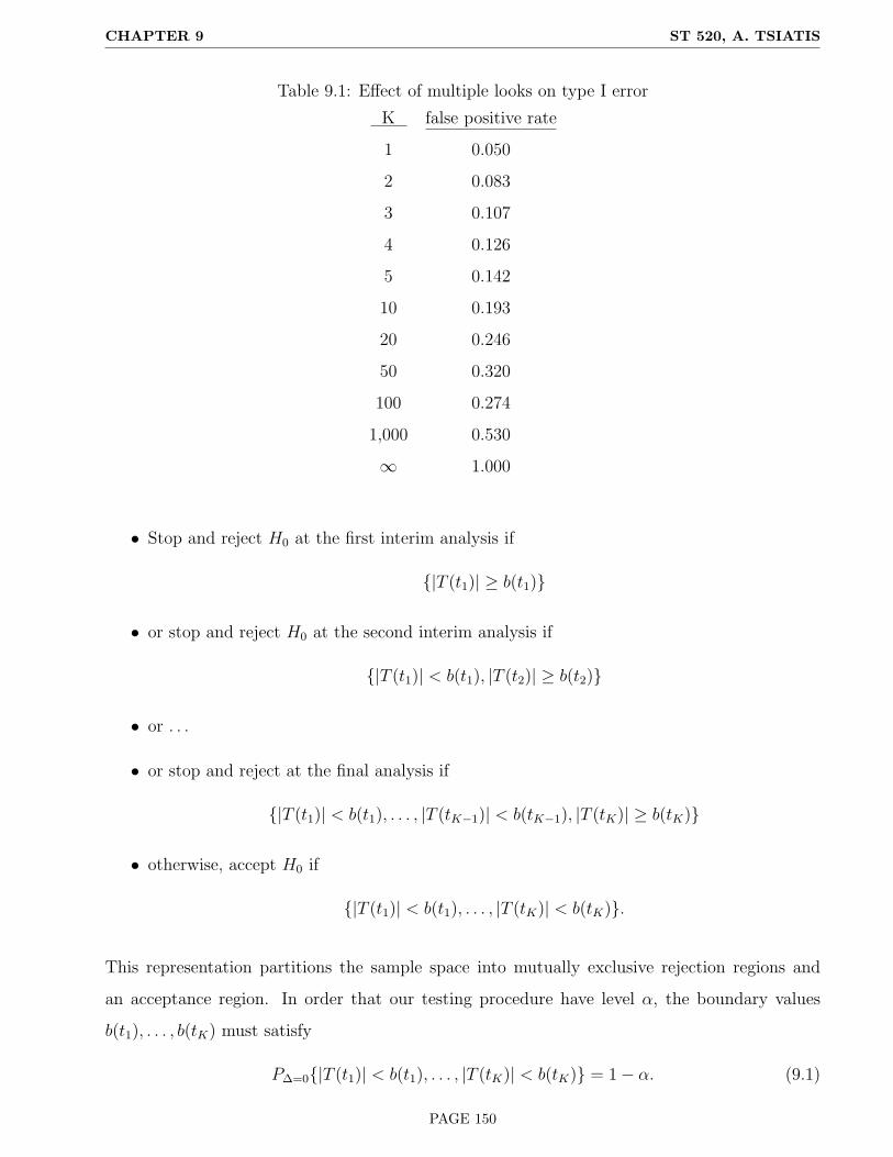
This is illustrated in the following table:

The last entry in this table was described by J. Cornfield as

“Sampling to a foregone conclusion”.

Our first objective is to derive group-sequential tests (i.e. choice of boundaries b(t1), . . . , b(tK))

that have the desired prespecified type I error of α.

Level α test

We want the probability of rejecting H0, when H0 is true, to be equal to α, say .05. The strategy

for rejecting or accepting H0 is as follows:

PAGE 149


Table 9.1: Effect of multiple looks on type I error

K false positive rate

1 0.050

2 0.083

3 0.107

4 0.126

5 0.142

10 0.193

20 0.246

50 0.320

100 0.274

1,000 0.530

∞ 1.000

• Stop and reject H0 at the first interim analysis if

{|T (t1)| ≥ b(t1)}

• or stop and reject H0 at the second interim analysis if

{|T (t1)| < b(t1), |T (t2)| ≥ b(t2)}

• or . . .

• or stop and reject at the final analysis if

{|T (t1)| < b(t1), . . . , |T (tK−1)| < b(tK−1), |T (tK)| ≥ b(tK)}

• otherwise, accept H0 if

{|T (t1)| < b(t1), . . . , |T (tK)| < b(tK)}.

This representation partitions the sample space into mutually exclusive rejection regions and

an acceptance region. In order that our testing procedure have level α, the boundary values

b(t1), . . . , b(tK) must satisfy

P∆=0{|T (t1)| < b(t1), . . . , |T (tK)| < b(tK)} = 1− α. (9.1)

PAGE 150


Remark:

By construction, the test statistic T (tj) will be approximately distributed as a standard nor-

mal, if the null hypothesis is true, at each time point tj. However, to ensure that the group-

sequential test have level α, the equality given by (9.1) must be satisfied. The probability on

the left hand side of equation (9.1) involves the joint distribution of the multivariate statistic

(T (t1), . . . , T (tK)). Therefore, we would need to know the joint distribution of this sequentially

computed test statistic at times t1, . . . , tK , under the null hypothesis, in order to compute the

necessary probabilities to ensure a level α test. Similarly, we would need to know the joint dis-

tribution of this multivariate statistic, under the alternative hypothesis to compute the power of

such a group-sequential test.

The major result which allows the use of a general methodology for monitoring clinical trials is

that

“Any efficient based test or estimator for ∆, properly normalized, when computed se-

quentially over time, has, asymptotically, a normal independent increments process

whose distribution depends only on the parameter ∆ and the statistical informa-

tion.”

Scharfstein, Tsiatis and Robins (1997). JASA. 1342-1350.

As we mentioned earlier the test statistics are constructed so that when ∆ = ∆∗

T (t) =∆̂(t)

se{∆̂(t)}∼ N(∆∗I1/2(t,∆∗), 1),

where we can approximate statistical information I(t,∆∗) by [se{∆̂(t)}]−2. If we normalize by

multiplying the test statistic by the square-root of the information; i.e.

W (t) = I1/2(t,∆∗)T (t),

then this normalized statistic, computed sequentially over time, will have the normal independent

increments structure alluded to earlier. Specifically, if we compute the statistic at times t1 <

t2 < . . . < tK , then the joint distribution of the multivariate vector {W (t1), . . . ,W (tK)} is

asymptotically normal with mean vector {∆∗I(t1,∆∗), . . . ,∆∗I(tK ,∆

∗)} and covariance matrix

where

var{W (tj)} = I(tj,∆∗), j = 1, . . . , K

PAGE 151


and

cov[W (tj), {W (tℓ)−W (tj)}] = 0, j < ℓ, j, ℓ = 1, . . . , K.

That is

• The statistic W (tj) has mean and variance proportional to the statistical information at

time tj

• Has independent increments; that is

W (t1) = W (t1)

W (t2) = W (t1) + {W (t2)−W (t1)}

·

·

·

W (tj) = W (t1) + {W (t2)−W (t1)}+ . . .+ {W (tj)−W (tj−1)}

has the same distribution as a partial sum of independent normal random variables

This structure implies that the covariance matrix of {W (t1), . . . ,W (tK)} is given by

var{W (tj)} = I(tj,∆∗), j = 1, . . . , K

and for j < ℓ

cov{W (tj),W (tℓ)}

= cov[W (tj), {W (tℓ)−W (tj)}+W (tj)]

= cov[W (tj), {W (tℓ)−W (tj)}] + cov{W (tj),W (tj)}

= 0 + var{W (tj)}

= I(tj,∆∗).

Since the test statistic

T (tj) = I−1/2(tj,∆∗)W (tj), j = 1, . . . , K

this implies that the joint distribution of {T (t1), . . . , T (tK)} is also multivariate normal where

the mean

E{T (tj)} = ∆∗I1/2(tj,∆∗), j = 1, . . . , K (9.2)

PAGE 152


and the covariance matrix is such that

var{T (tj)} = 1, j = 1, . . . , K (9.3)

and for j < ℓ, the covariances are

cov{T (tj), T (tℓ)} = cov{I−1/2(tj,∆∗)W (tj), I

−1/2(tℓ,∆∗)W (tℓ)}

= I−1/2(tj,∆∗)I−1/2(tℓ,∆

∗)cov{W (tj),W (tℓ)}

= I−1/2(tj,∆∗)I−1/2(tℓ,∆

∗)I(tj,∆∗)

=I1/2(tj,∆

∗)

I1/2(tℓ,∆∗)=

√√√√I(tj,∆∗)

I(tℓ,∆∗). (9.4)

In words, the covariance of T (tj) and T (tℓ) is the square-root of the relative information at times

tj and tℓ. Hence, under the null hypothesis ∆ = 0, the sequentially computed test statistic

{T (t1), . . . , T (tK)} is multivariate normal with mean vector zero and covariance matrix (in this

case the same as the correlation matrix, since the variances are all equal to one)

VT =

√√√√I(tj, 0)

I(tℓ, 0)

, j ≤ ℓ. (9.5)

The importance of this result is that the joint distribution of the sequentially computed test statis-

tic, under the null hypothesis, is completely determined by the relative proportion of information

at each of the monitoring times t1, . . . , tK . This then allows us to evaluate probabilities such as

those in equation (9.1) that are necessary to find appropriate boundary values b(t1), . . . , b(tK)

that achieve the desired type I error of α.

9.3.1 Equal increments of information

Let us consider the important special case where the test statistic is computed after equal incre-

ments of information; that is

I(t1, ·) = I, I(T2, ·) = 2I, . . . , I(tK , ·) = KI.

Remark: For problems where the response of interest is instantaneous, whether this response be

discrete or continuous, the information is proportional to the number of individuals under study.

In such cases, calculating the test statistic after equal increments of information is equivalent to

PAGE 153


calculating the statistic after equal number of patients have entered the study. So, for instance, if

we planned to accrue a total of 100 patients with the goal of comparing the response rate between

two treatments, we may wish to monitor five times after equal increments of information; i.e after

every 20 patients enter the study.

In contrast, if we were comparing the survival distributions with possibly right censored data,

then it turns out that information is directly proportional to the number of deaths. Thus, for

such a study, monitoring after equal increments of information would correspond to conducting

interim analyses after equal number of observed deaths.

In any case, monitoring a study K times after equal increments of information imposes a

very specific distributional structure, under the null hypothesis, for the sequentially com-

puted test statistic that can be exploited in constructing group-sequential tests. Because

I(tj, 0) = jI, j = 1, . . . , K, this means that the joint distribution of the sequentially com-

puted test statistic {T (t1), . . . , T (tK)} is a multivariate normal with mean vector equal to zero

and by (9.5) with a covariance matrix equal to

VT =

√√√√I(tj, 0)

I(tℓ, 0)=

√j

ℓ

, j ≤ ℓ. (9.6)

This means that under the null hypothesis the joint distribution of the sequentially computed

test statistic computed after equal increments of information is completely determined once we

know the total number K of interim analyses that are intended. Now, we are in a position to

compute probabilities such as

P∆=0{|T (t1)| < b1, . . . , |T (tK)| < bK}

in order to determine boundary values b1, . . . , bK where the probability above equals 1 − α as

PAGE 154


would be necessary for a level-α group-sequential test.

PAGE 155


Remark: The computations necessary to compute such integrals of multivariate normals with

the covariance structure (9.6) can be done quickly using using recursive numerical integration

that was first described by Armitage, McPherson and Rowe (1969). This method takes advantage

of the fact that the joint distribution is that of a standardized partial sum of independent normal

random variables. This integration allows us to search for different combinations of b1, . . . , bK

which satisfy

P∆=0{|T (t1)| < b1, . . . , |T (tK)| < bK} = 1− α.

There are infinite combinations of such boundary values that lead to level-α tests; thus, we need

to assess the statistical consequences of these different combinations to aid us in making choices

in which to use.

9.4 Choice of boundaries

Let us consider the flexible class of boundaries proposed by Wang and Tsiatis (1987) Biometrics.

For the time being we will restrict attention to group-sequential tests computed after equal

increments of information and later discuss how this can be generalized. The boundaries by

Wang and Tsiatis were characterized by a power function which we will denote by Φ. Specifically,

we will consider boundaries where

bj = (constant)× j(Φ−.5), .

Different values of Φ will characterize different shapes of boundaries over time. We will also refer

to Φ as the shape parameter.

For any value Φ, we can numerically derive the the constant necessary to obtain a level-α test.

Namely, we can solve for the value c such that

P∆=0{K⋂

j=1

|T (tj)| < cj(Φ−.5)} = 1− α.

Recall. Under the null hypothesis, the joint distribution of {T (t1), . . . , T (tK)} is completely

known if the times t1, . . . , tK are chosen at equal increments of information. The above integral

is computed for different c until we solve the above equation. That a solution exists follows from

the monotone relationship of the above probability as a function of c. The resulting solution will

be denoted by c(α,K,Φ). Some of these are given in the following table.

PAGE 156


Table 9.2: Group-sequential boundaries for two-sided tests for selected values of α, K, Φ

K

Φ 2 3 4 5

α = .05

0.0 2.7967 3.4712 4.0486 4.5618

0.1 2.6316 3.1444 3.5693 3.9374

0.2 2.4879 2.8639 3.1647 3.4175

0.3 2.3653 2.6300 2.8312 2.9945

0.4 2.2636 2.4400 2.5652 2.6628

0.5 2.1784 2.2896 2.3616 2.4135

α = .01

0.0 3.6494 4.4957 5.2189 5.8672

0.1 3.4149 4.0506 4.5771 5.0308

0.2 3.2071 3.6633 4.0276 4.3372

0.3 3.0296 3.3355 3.5706 3.7634

0.4 2.8848 3.0718 3.2071 3.3137

0.5 2.7728 2.8738 2.9395 2.9869

Examples: Two boundaries that have been discussed extensively in the literature and have been

used in many instances are special cases of the class of boundaries considered above. These are

when Φ = .5 and Φ = 0. The first boundary when Φ = .5 is the Pocock boundary; Pocock (1977)

Biometrika and the other when Φ = 0 is the O’Brien-Fleming boundary; O’Brien and Fleming

(1979) Biometrics.

9.4.1 Pocock boundaries

The group-sequential test using the Pocock boundaries rejects the null hypothesis at the first

interim analysis time tj, j = 1, . . . , K (remember equal increments of information) that

|T (tj)| ≥ c(α,K, 0.5), j = 1, . . . , K.

That is, the null hypothesis is rejected at the first time that the standardized test statistic using

all the accumulated data exceeds some constant.

PAGE 157


For example, if we take K = 5 and α = .05, then according to Table 10.2 c(.05, 5, 0.5) = 2.41.

Therefore, the .05 level test which will be computed a maximum of 5 times after equal increments

of information will reject the null hypothesis at the first time that the standardized test statistic

exceeds 2.41; that is, we reject the null hypothesis at the first time tj, j = 1, . . . , 5 when |T (tj)| ≥2.41. This is also equivalent to rejecting the null hypothesis at the first time tj, j = 1, . . . , 5 that

the nominal p-value is less than .0158.

9.4.2 O’Brien-Fleming boundaries

The O’Brien-Fleming boundaries have a shape parameter Φ = 0. A group-sequential test using

the O’Brien-Fleming boundaries will reject the null hypothesis at the first time tj, j = 1, . . . , K

when

|T (tj)| ≥ c(α,K, 0.0)/√j, j = 1, . . . , K.

For example, if we again choose K = 5 and α = .05, then according to Table 10.2 c(.05, 5, 0.0) =

4.56. Therefore, using the O’Brien-Fleming boundaries we would reject at the first time tj, j =

1, . . . , 5 when

|T (tj)| ≥ 4.56/√j, j = 1, . . . , 5.

Therefore, the five boundary values in this case would be b1 = 4.56, b2 = 3.22, b3 = 2.63,

b4 = 2.28, and b5 = 2.04

The nominal p-values for the O’Brien-Fleming boundaries are contrasted to those from the

Pocock boundaries, for K = 5 and α = .05 in the following table.

Table 9.3: Nominal p-values for K = 5 and α = .05

Nominal p-value

j Pocock O’Brien-Fleming

1 0.0158 0.000005

2 0.0158 0.00125

3 0.0158 0.00843

4 0.0158 0.0225

5 0.0158 0.0413

PAGE 158


The shape of these boundaries are also contrasted in the following figure.

Figure 9.1: Pocock and O’Brien-Fleming Boundaries

Interim Analysis Time

Bou

nday

1 2 3 4 5

-6-4

-20

24

6

PocockO’Brien-Fleming

PAGE 159


9.5 Power and sample size in terms of information

We have discussed the construction of group-sequential tests that have a pre-specified level of

significance α. We also need to consider the effect that group-sequential tests have on power and

its implications on sample size. To set the stage, we first review how power and sample size are

determined with a single analysis using information based criteria.

As shown earlier, the distribution of the test statistic computed at a specific time t; namely T (t),

under the null hypothesis, is

T (t)∆=0∼ N(0, 1)

and for a clinically important alternative, say ∆ = ∆A is

T (t)∆=∆A∼ N(∆AI

1/2(t,∆A), 1),

where I(t,∆A) denotes statistical information which can be approximated by [se{∆̂(t)}]−2, and

∆AI1/2(t,∆A) is the noncentrality parameter. In order that a two-sided level-α test have power

1− β to detect the clinically important alternative ∆A, we need the noncentrality parameter

∆AI1/2(t,∆A) = Zα/2 + Zβ,

or

I(t,∆A) =

{Zα/2 + Zβ

∆A

}2

. (9.7)

From this relationship we see that the power of the test is directly dependent on statistical

information. Since information is approximated by [se{∆̂(t)}]−2, this means that the study

should collect enough data to ensure that

[se{∆̂(t)}]−2 =

{Zα/2 + Zβ

∆A

}2

.

Therefore one strategy that would guarantee the desired power to detect a clinically important

difference is to monitor the standard error of the estimated difference through time t as data

were being collected and to conduct the one and only final analysis at time tF where

[se{∆̂(tF )}]−2 =

{Zα/2 + Zβ

∆A

}2

using the test which rejects the null hypothesis when

|T (tF )| ≥ Zα/2.

PAGE 160


Remark Notice that we didn’t have to specify any of the nuisance parameters with this

information-based approach. The accuracy of this method to achieve power depends on how

good the approximation of the distribution of the test statistic is to a normal distribution and

how good the approximation of [se{∆̂(tF )}]−2 is to the Fisher information. Some preliminary

numerical simulations have shown that this information-based approach works very well if the

sample sizes are sufficiently large as would be expected in phase III clinical trials.

In actuality, we cannot launch into a study and tell the investigators to keep collecting data until

the standard error of the estimated treatment difference is sufficiently small (information large)

without giving them some idea how many resources they need (i.e. sample size, length of study,

etc.). Generally, during the design stage, we posit some guesses of the nuisance parameters and

then use these guesses to come up with some initial design.

For example, if we were comparing the response rate between two treatments, say treatment 1

and treatment 0, and were interested in the treatment difference π1 − π0, where πj denotes the

population response probability for treatment j = 0, 1, then, at time t, we would estimate the

treatment difference using ∆̂(t) = p1(t)− p0(t), where pj(t) denotes the sample proportion that

respond to treatment j among the individuals assigned to treatment j by time t for j = 0, 1.

The standard error of ∆̂(t) = p1(t)− p0(t) is given by

se{∆̂(t)} =

√√√√π1(1− π1)

n1(t)+π0(1− π0)

n0(t).

Therefore, to obtain the desired power of 1 − β to detect the alternative where the population

response rates were π1 and π0, with π1 − π0 = ∆A, we would need the sample sizes n1(tF ) and

n0(tF ) to satisfy {

π1(1− π1)

n1(tF )+π0(1− π0)

n0(tF )

}−1

=

{Zα/2 + Zβ

∆A

}2

.

Remark: The sample size formula given above is predicated on the use of the test statistic

T (t) =p1(t)− p0(t)√

p1(t){1−p1(t)}n1(t)

+ p0(t){1−p0(t)}n0(t)

to test for treatment difference in the response rates. Strictly speaking, this is not the same as

the proportions test

T (t) =p1(t)− p0(t)√

p̄(t){1− p̄(t)}{

1n1(t)

+ 1n0(t)

} ,

PAGE 161


although the difference between the two tests is inconsequential with equal randomization and

large samples. What we discussed above is essentially the approach taken for sample size calcu-

lations used in Chapter 6 of the notes. The important point here is that power is driven by the

amount of statistical information we have regarding the parameter of interest from the available

data. The more data the more information we have. To achieve power 1 − β to detect the

clinically important difference ∆A using a two-sided test at the α level of significance means that

we need to have collected enough data so that the statistical information equals

{Zα/2 + Zβ

∆A

}2

.

Let us examine how issues of power and information relate to group-sequential tests. If we are

planning to conduct K interim analyses after equal increments of information, then the power

of the group-sequential test to detect the alternative ∆ = ∆A is given by

1− P∆=∆A{|T (t1)| < b1, . . . , |T (tK)| < bK}.

In order to compute probabilities of events such as that above we need to know the joint distri-

bution of the vector {T (t1), . . . , T (tK)} under the alternative hypothesis ∆ = ∆A.

It will be useful to consider the maximum information at the final analysis which we will denote

asMI. A K-look group-sequential test with equal increments of information and with maximum

informationMI would have interim analyses conducted at times tj where j×MI/K information

has occurred; that is,

I(tj,∆A) = j ×MI/K, j = 1, . . . , K. (9.8)

Using the results (9.2)-(9.4) and (9.8) we see that the joint distribution of {T (t1), . . . , T (tK)},under the alternative hypothesis ∆ = ∆A, is a multivariate normal with mean vector

∆A

√j ×MI

K, j = 1, . . . , K

and covariance matrix VT given by (9.6). If we define

δ = ∆A

√MI,

then the mean vector is equal to

(δ

√1

K, δ

√2

K, . . . , δ

√K − 1

K, δ). (9.9)

PAGE 162


A group-sequential level-α test from the Wang-Tsiatis family rejects the null hypothesis at the

first time tj, j = 1, . . . , K where

|T (tj)| ≥ c(α,K,Φ)j(Φ−.5).

For the alternative HA : ∆ = ∆A and maximum information MI, the power of this test is

1− Pδ[K⋂

j=1

{|T (tj)| < c(α,K,Φ)j(Φ−.5)}],

where δ = ∆A

√MI, and {T (t1), . . . , T (tK)} is multivariate normal with mean vector (9.9) and

covariance matrix VT given by (9.6). For fixed values of α, K, and Φ, the power is an increasing

function of δ which can be computed numerically using recursive integration. Consequently, we

can solve for the value δ that gives power 1− β above. We denote this solution by δ(α,K,Φ, β).

Remark: The value δ plays a role similar to that of a noncentrality parameter.

Since δ = ∆A

√MI, this implies that a group-sequential level-α test with shape parameter Φ,

computed at equal increments of information up to a maximum of K times needs the maximum

information to equal

∆A

√MI = δ(α,K,Φ, β)

or

MI =

{δ(α,K,Φ, β)

∆A

}2

to have power 1− β to detect the clinically important alternative ∆ = ∆A.

9.5.1 Inflation Factor

A useful way of thinking about the maximum information that is necessary to achieve prespecified

power with a group-sequential test is to relate this to the information necessary to achieve

prespecified power with a fixed sample design. In formula (9.7), we argued that the information

necessary to detect the alternative ∆ = ∆A with power 1− β using a fixed sample test at level

α is

IFS =

{Zα/2 + Zβ

∆A

}2

.

PAGE 163


In contrast, the maximum information necessary at the same level and power to detect the same

alternative using a K-look group-sequential test with shape parameter Φ is

MI =

{δ(α,K,Φ, β)

∆A

}2

.

Therefore

MI =

{Zα/2 + Zβ

∆A

}2 {δ(α,K,Φ, β)

Zα/2 + Zβ

}2

= IFS × IF (α,K,Φ, β),

where

IF (α,K,Φ, β) =

{δ(α,K,Φ, β)

Zα/2 + Zβ

}2

is the inflation factor, or the relative increase in information necessary for a group-sequential test

to have the same power as a fixed sample test.

Note: The inflation factor does not depend on the endpoint of interest or the magnitude of the

treatment difference that is considered clinically important. It only depends on the level (α),

power (1− β), and the group-sequential design (K,Φ). The inflation factors has been tabulated

for some of the group-sequential tests which are given in the following table.

PAGE 164


Table 9.4: Inflation factors as a function of K, α, β and the type of boundary

α=0.05 α=0.01

Power=1-β Power=1-β

K Boundary 0.80 0.90 0.95 0.80 0.90 0.95

2 Pocock 1.11 1.10 1.09 1.09 1.08 1.08

O-F 1.01 1.01 1.01 1.00 1.00 1.00

3 Pocock 1.17 1.15 1.14 1.14 1.12 1.12

O-F 1.02 1.02 1.02 1.01 1.01 1.01

4 Pocock 1.20 1.18 1.17 1.17 1.15 1.14

O-F 1.02 1.02 1.02 1.01 1.01 1.01

5 Pocock 1.23 1.21 1.19 1.19 1.17 1.16

O-F 1.03 1.03 1.02 1.02 1.01 1.01

6 Pocock 1.25 1.22 1.21 1.20 1.19 1.17

O-F 1.03 1.03 1.03 1.02 1.02 1.02

7 Pocock 1.26 1.24 1.22 1.22 1.20 1.18

O-F 1.03 1.03 1.03 1.02 1.02 1.02

This result is convenient for designing studies which use group-sequential stopping rules as it

can build on techniques for sample size computations used traditionally for fixed sample tests.

For example, if we determined that we needed to recruit 500 patients into a study to obtain

some prespecified power to detect a clinically important treatment difference using a traditional

fixed sample design, where information, say, is proportional to sample size, then in order that

we have the same power to detect the same treatment difference with a group-sequential test

we would need to recruit a maximum number of 500 × IF patients, where IF denotes the

corresponding inflation factor for that group-sequential design. Of course, interim analyses would

be conducted after every 500×IFK

patients had complete response data, a maximum of K times,

with the possibility that the trial could be stopped early if any of the interim test statistics

exceeded the corresponding boundary. Let us illustrate with a specific example.

Example with dichotomous endpoint

Let π1 and π0 denote the population response rates for treatments 1 and 0 respectively. Denote

PAGE 165


the treatment difference by ∆ = π1−π0 and consider testing the null hypothesisH0 : ∆ = 0 versus

the two-sided alternative HA : ∆ 6= 0. We decide to use a 4-look O’Brien-Fleming boundary; i.e.

K = 4 and Φ = 0, at the .05 level of significance (α = .05). Using Table 10.2, we derive the

boundaries which correspond to rejecting H0 whenever

|T (tj)| ≥ 4.049/√j, j = 1, . . . , 4.

The boundaries are given by

Table 9.5: Boundaries for a 4-look O-F test

j bj nominal p-value

1 4.05 .001

2 2.86 .004

3 2.34 .019

4 2.03 .043

In designing the trial, the investigators tell us that they expect the response rate on the control

treatment (treatment 0) to be about .30 and want to have at least 90% power to detect a

significant difference if the new treatment increases the response by .15 (i.e. from .30 to .45)

using a two-sided test at the .05 level of significance. They plan to conduct a two arm randomized

study with equal allocation and will test the null hypothesis using the standard proportions test.

The traditional fixed sample size calculations using the methods of chapter six, specifically for-

mula (6.4), results in the desired fixed sample size of

nFS =

1.96 + 1.28

√.3×.7+.45×.552×.375×.625

.15

2

× 4× .375× .625 = 434,

or 217 patients per treatment arm.

Using the inflation factor from Table 10.4 for the 4-look O’Brien-Fleming boundaries at the

.05 level of significance and 90% power i.e. 1.02, we compute the maximum sample size of

434 × 1.02=444, or 222 per treatment arm. To implement this design, we would monitor the

data after every 222/4 ≈ 56 individuals per treatment arm had complete data regarding their

response for a maximum of four times. At each of the four interim analyses we would compute

PAGE 166


the test statistic, i.e. the proportions test

T (tj) =p1(tj)− p0(tj)√

p̄(tj){1− p̄(tj)}{

1n1(tj)

+ 1n0(tj)

} ,

using all the data accumulated up to the j-th interim analysis. If at any of the four interim anal-

yses the test statistic exceeded the corresponding boundary given in Table 10.5 or, equivalently,

if the two-sided p-value was less than the corresponding nominal p-value in Table 10.5, then we

would reject H0. If we failed to reject at all four analyses we would then accept H0.

9.5.2 Information based monitoring

In the above example it was assumed that the response rate on the control treatment arm was .30.

This was necessary for deriving sample sizes. It may be, in actuality, that the true response rate

for the control treatment is something different, but even so, if the new treatment can increase

the probability of response by .15 over the control treatment we may be interested in detecting

such a difference with 90% power. We’ve argued that power is directly related to information.

For a fixed sample design, the information necessary to detect a difference ∆ = .15 between the

response probabilities of two treatments with power 1 − β using a two-sided test at the α level

of significance is {Zα/2 + Zβ

∆A

}2

.

For our example, this equals {1.96 + 1.28

.15

}2

= 466.6.

For a 4-look O-F design this information must be inflated by 1.02 leading toMI = 466.6×1.02 =

475.9. With equal increments, this means that an analysis should be conducted at times tj when

the information equals j×475.94

= 119 × j, j = 1, . . . , 4. Since information is approximated by

[se{∆̂(t)}]−2, and in this example (comparing two proportions) is equal to

[p1(t){1− p1(t)}

n1(t)+p0(t){1− p0(t)}

n0(t)

]−1

,

we could monitor the estimated standard deviation of the treatment difference estimator and

conduct the four interim analyses whenever

[se{∆̂(t)}]−2 = 119× j, j = 1, . . . , 4,

PAGE 167


i.e. at times tj such that

[p1(tj){1− p1(tj)}

n1(tj)+p0(tj){1− p0(tj)}

n0(tj)

]−1

= 119× j, j = 1, . . . , 4.

At each of the four analysis times we would compute the test statistic T (tj) and reject H0 at the

first time that the boundary given in Table 10.5 was exceeded.

This information-based procedure would yield a test that has the correct level of significance

(α = .05) and would have the desired power (1 − β = .90) to detect a treatment difference

of .15 in the response rates regardless of the underlying true control treatment response rate

π0. In contrast, if we conducted the analysis after every 112 patients (56 per treatment arm),

as suggested by our preliminary sample size calculations, then the significance level would be

correct under H0 but the desired power would be achieved only if our initial guess (i.e. π0 = .30)

were correct. Otherwise, we would over power or under power the study depending on the true

value of π0 which, of course, is unknown to us.

9.5.3 Average information

We still haven’t concluded which of the proposed boundaries (Pocock, O-F, or other shape

parameter Φ) should be used. If we examine the inflation factors in Table 10.4 we notice that K-

look group-sequential tests that use the Pocock boundaries require greater maximum information

that do K-look group-sequential tests using the O-F boundaries at the same level of significance

and power; but at the same time we realize that Pocock tests have a better chance of stopping

early than O-F tests because of the shape of the boundary. How do we assess the trade-offs?

One way is to compare the average information necessary to stop the trial between the different

group-sequential tests with the same level and power. A good group-sequential design is one

which has a small average information.

Remark: Depending on the endpoint of interest this may translate to smaller average sample

size or smaller average number of events, for example.

How do we compute average information?

We have already discussed that the maximum information MI is obtained by computing the

PAGE 168


information necessary to achieve a certain level of significance and power for a fixed sample

design and multiplying by an inflation factor. For designs with a maximum of K analyses after

equal increments of information, the inflation factor is a function of α (the significance level), β

(the type II error or one minus power), K, and Φ (the shape parameter of the boundary). We

denote this inflation factor by IF (α,K,Φ, β).

Let V denote the number of interim analyses conducted before a study is stopped. V is a discrete

integer-valued random variable that can take on values from 1, . . . , K. Specifically, for a K-look

group-sequential test with boundaries b1, . . . , bK , the event V = j (i.e. stopping after the j-th

interim analysis) corresponds to

(V = j) = {|T (t1)| < b1, . . . , |T (tj−1)| < bj−1, |T (tj)| ≥ bj}, j = 1, . . . , K.

The expected number of interim analyses for such a group-sequential test, assuming ∆ = ∆∗ is

given by

E∆∗(V ) =K∑

j=1

j × P∆∗(V = j).

Since each interim analysis is conducted after incrementsMI/K of information, this implies that

the average information before a study is stopped is given by

AI(∆∗) =MI

KE∆∗(V ).

Since MI = IFS × IF (α,K,Φ, β), then

AI(α,K,Φ, β,∆∗) = IFS

[{IF (α,K,Φ, β)

K

}E∆∗(V )

].

Note: We use the notation AI(α,K,Φ, β,∆∗) to emphasize the fact that the average information

depends on the level, power, maximum number of analyses, boundary shape, and alternative of

interest. For the most part we will consider the average information at the null hypothesis ∆∗ = 0

and the clinically important alternative ∆∗ = ∆A. However, other values of the parameter may

also be considered.

Using recursive numerical integration, the E∆∗(V ) can be computed for different sequential de-

signs at the null hypothesis, at the clinically important alternative ∆A, as well as other values

for the treatment difference. For instance, if we take K = 5, α = .05, power equal to 90%,

then under HA : ∆ = ∆A, the expected number of interim analyses for a Pocock design is

PAGE 169


equal to E∆A(V ) = 2.83. Consequently, the average information necessary to stop a trial, if the

alternative HA were true would be

IFS

[{IF (.05, 5, .5, .10)

5

}× 2.83

]

= IFS{1.21

5× 2.83

}

= IFS × .68.

Therefore, on average, we would reject the null hypothesis using 68% of the information necessary

for a fixed-sample design with the same level (.05) and power (.90) as the 5-look Pocock design, if

indeed, the clinically important alternative hypothesis were true. This is why sequential designs

are sometimes preferred over fixed-sample designs.

Remark: If the null hypothesis were true, then it is unlikely (< .05) that the study would be

stopped early with the sequential designs we have been discussing. Consequently, the average

information necessary to stop a study early if the null hypothesis were true would be close to the

maximum information (i.e. for the 5-look Pocock design discussed above we would need almost

21% more information than the corresponding fixed-sample design).

In contrast, if we use the 5-look O-F design with α = .05 and power of 90%, then the expected

number of interim analyses equals E∆A(V ) = 3.65 under the alternative hypothesis HA. Thus,

the average information is

IFS

[{IF (.05, 5, 0.0, .10)

5

}× 3.65

]

= IFS{1.03

5× 3.65

}

= IFS × .75.

PAGE 170


Summarizing these results: For tests at the .05 level of significance and 90% power, we have

Maximum Average

Designs information information (HA)

5-look Pocock IFS × 1.21 IFS × .68

5-look O-F IFS × 1.03 IFS × .75

Fixed-sample IFS IFS

Recall:

IFS =

{Zα/2 + Zβ

∆A

}2

.

Remarks:

• If you want a design which, on average, stops the study with less information when there

truly is a clinically important treatment difference, while preserving the level and power of

the test, then a Pocock boundary is preferred to the O-F boundary.

• By a numerical search, one can derive the “optimal” shape parameter Φ which minimizes

the average information under the clinically important alternative ∆A for different values

of α, K, and power (1 − β). Some these optimal Φ are provided in the paper by Wang

and Tsiatis (1987) Biometrics. For example, when K = 5, α = .05 and power of 90% the

optimal shape parameter Φ = .45, which is very close to the Pocock boundary.

• Keep in mind, however, that the designs with better stopping properties under the alter-

native need greater maximum information which, in turn, implies greater information will

be needed if the null hypothesis were true.

• Most clinical trials with a monitoring plan seem to favor more “conservative” designs such

as the O-F design.

Statistical Reasons

1. Historically, most clinical trials fail to show a significant difference; hence, from a global

perspective it is more cost efficient to use conservative designs.

PAGE 171


2. Even a conservative design, such as O-F, results in a substantial reduction in average

information, under the alternative HA, before a trial is completed as compared to a fixed-

sample design (in our example .75 average information) with only a modest increase in the

maximum information (1.03 in our example).

Non-statistical Reasons

3. In the early stages of a clinical trial, the data are less reliable and possibly unrepresentative

for a variety of logistical reasons. It is therefore preferable to make it more difficult to stop

early during these early stages.

4. Psychologically, it is preferable to have a nominal p-value at the end of the study which

is close to .05. The nominal p-value at the final analysis for the 5-look O-F test is .041

as compare to .016 for the 5-look Pocock test. This minimizes the embarrassing situation

where, say, a p-value of .03 at the final analysis would have to be declared not significant

for those using a Pocock design.

9.5.4 Steps in the design and analysis of group-sequential tests with equal incre-

ments of information

Design

1. Decide the maximum number of looks K and the boundary Φ. We’ve already argued the

pros and cons of conservative boundaries such as O-F versus more aggressive boundaries such

as Pocock. As mentioned previously, for a variety of statistical and non-statistical reasons,

conservative boundaries have been preferred in practice. In terms of the number of looks K, it

turns out that the properties of a group-sequential test is for the most part insensitive to the

number of looks after a certain point. We illustrate this point using the following table which

looks at the maximum information and the average information under the alternative for the

O’Brien-Fleming boundaries for different values of K.

PAGE 172


Table 9.6: O’Brien-Fleming boundaries (Φ = 0); α = .05, power=.90

Maximum Average

K Information Information (HA)

1 IFS IFS

2 IFS × 1.01 IFS × .85

3 IFS × 1.02 IFS × .80

4 IFS × 1.02 IFS × .77

5 IFS × 1.03 IFS × .75

We note from Table 10.6 that there is little change in the early stopping properties of the group-

sequential test once K exceeds 4. Therefore, the choice of K should be chosen based on logistical

and practical issues rather than statistical principles (as long as K exceeds some lower threshold;

i.e. 3 or 4). For example, the choice might be determined by how many times one can feasibly

get a data monitoring committee to meet.

2. Compute the information necessary for a fixed sample design and translate this into a physical

design of resource use. You will need to posit some initial guesses for the values of the nuisance

parameters as well as defining the clinically important difference that you want to detect with

specified power using a test at some specified level of significance in order to derive sample sizes

or other design characteristics. This is the usual “sample size considerations” that were discussed

throughout the course.

3. The fixed sample information must be inflated by the appropriate inflation factor IF (α,K,Φ, β)

to obtain the maximum information

MI = IFS × IF (α,K,Φ, β).

Again, this maximum information must be translated into a feasible resource design using initial

guesses about the nuisance parameters. For example, if we are comparing the response rates of

a dichotomous outcome between two treatments, we generally posit the response rate for the

control group and we use this to determine the required sample sizes as was illustrated in the

example of section 10.5.1.

PAGE 173


Analysis

4. After deriving the maximum information (most often translated into a maximum sample size

based on initial guesses), the actual analyses will be conducted a maximum of K times after

equal increments of MI/K information.

Note: Although information can be approximated by [se{∆̂(t)}]−2, in practice, this is not gen-

erally how the analysis times are determined; but rather, the maximum sample size (determined

based on best initial guesses) is divided by K and analyses are conducted after equal increments

of sample size. Keep in mind, that this usual strategy may be under or over powered if the initial

guesses are incorrect.

5. At the j-th interim analysis, the standardized test statistic

T (tj) =∆̂(tj)

se{∆̂(tj)},

is computed using all the data accumulated until that time and the null hypothesis is rejected

the first time the test statistic exceeds the corresponding boundary value.

Note: The procedure outlined above will have the correct level of significance as long as the

interim analyses are conducted after equal increments of information. So, for instance, if we

have a problem where information is proportional to sample size, then as long as the analyses

are conducted after equal increments of sample size we are guaranteed to have the correct type

I error. Therefore, when we compute sample sizes based on initial guesses for the nuisance

parameters and monitor after equal increments of this sample size, the corresponding test has

the correct level of significance under the null hypothesis.

However, in order that this test have the correct power to detect the clinically important difference

∆A, it must be computed after equal increments of statistical information MI/K where

MI =

{Zα/2 + Zβ

∆A

}2

IF (α,K,Φ, β).

If the initial guesses were correct, then the statistical information obtained from the sample

sizes (derived under these guesses) corresponds to that necessary to achieve the correct power.

If, however, the guesses were incorrect, then the resulting test may be under or over powered

depending on whether there is less or more statistical information associated with the given

sample size.

PAGE 174


Although an information-based monitoring strategy, such as that outlined in section 10.5.2, is

not always practical, I believe that information (i.e. [se{∆̂(t)}]−2) should also be monitored as

the study progresses and if this deviates substantially from that desired, then the study team

should be made aware of this fact so that possible changes in design might be considered. The

earlier in the study that problems are discovered, the easier they are to fix.

PAGE 175

9 early stopping of clinical trials - nc state university 9 st 520, a. tsiatis 9 early stopping of...

Documents