pdf (cfd simulation of bed expansion and gas hold up behaviour
TRANSCRIPT

i
A
Project report
on
CFD simulation of Bed expansion and Gas hold up behaviour of Gas-Liquid-
Solid Fluidized Bed
Submitted by
LIPIKA KALO
Roll No. 210CH1263
In partial fulfillment of
Master of Technology (Chemical Engg.)
Under the Guidance of
DR. H.M. JENA
Department of Chemical Engineering
National Institute of Technology
Rourkela
2012

ii
National Institute of Technology
Rourkela
CERTIFICATE
This is to certify that the seminar report entitled, “CFD Simulation of Bed expansion and Gas
hold up behaviour of Gas-Liquid-Solid Fluidized Bed” submitted by Lipika Kalo (Roll No-
210CH1263 ) in partial fulfilment of the requirements of the degree of Master of Technology in
Chemical Engineering at National Institute of Technology, Rourkela is prepared by her under my
supervision and guidance.
Date:
DR. H. M. JENA
Dept. of Chemical Engineering
National Institute of Technology

iii
ACKNOWLEDGEMENT
I take this opportunity to express my sense of gratitude and indebtedness to
Dr. H.M. Jena, Department of Chemical Engineering for helping me a lot to
complete the seminar work without whose sincere and kind effort, this seminar
would not have been success.
Date: Lipika Kalo
Roll. No.: 210CH1263
4th Semester, M. Tech
Chemical Engineering

iv
CONTENTS
COVER PAGE
CERTIFICATE
ACKNOWLEDGEMENT
CONTENTS
ABSTRACT
LIST OF FIGURES
LIST OF TABLES
NOMENCLATURE
1.0 INTRODUCTION
1.1 Three phase fluidized bed
1.2 Advantages of Three-phase Fluidized Beds
1.3Application of Three phase fluidized bed
1.4 Drawbacks of Fluidized bed
1.5Modes of operation of Gas-Liquid-Solid Fluidized bed and Flow
Regimes
1.6 Variables affect the quality of Fluidization
1.7 Complexion of Three phase system
1.8 Present work
1.9 Thesis Layout
2.0 LITERATURE REVIEW
3.0 CFD MODELLING OF THREE PHASE FLUIDIZED BED
3.1 CFD (Computational Fluid Dynamics)
3.2 Advantages of CFD
3.3 Limitations of CFD
i
ii
iii
iv
vi
vii
ix
x
1
1
2
3
3
4
5
5
6
6
7
12
12
12
13

v
3.4 Applications of CFD
3.5 Working of CFD
3.6 Discretization Methods in CFD
3.7 Approaches to Multiphase modelling
3.8Computational Flow model
3.9Numerical Methodology
3.10 Phase Dynamics
3.11 Gas hold up
3.12 Bed Expansion
4.0 CONCLUSION
REFERENCES
13
14
16
18
21
22
25
26
37
39
40

vi
Abstract
Three-phase fluidization is a process used to bring into contact gas, liquid and solids, and in
which the solid particles are kept in suspension by a through flow of liquid. Three-phase
fluidized beds are used extensively in the refining, petrochemical, pharmaceutical,
biotechnology, food and environmental industries. The fundamental characteristics of a three-
phase fluidized bed have been recently studied extensively. The gas holdup is one of the most
important characteristics for analysing the performance of a three-phase fluidized bed. In the
present work FLUENT has been used to study gas-liquid-solid fluidization. CFD simulations
have been done for a column of height 1.88 m and diameter 0.1 m containing glass beads as solid
particles of size 2.18 mm. In the present work, involving three phase fluidized bed, CFD analysis
of gas holdup and bed expansion behaviour have been studied. ANSYS has been used to
generate a 3D fine grid. The gas (air) and liquid (water) is injected at the base with different
velocities.
vii
FIGURE NO.
3.1
3.2
3.3
3.4
3.5
3.6
3.7
3.8
LIST OF FIGURES
DESCRIPTION
3D mesh
Contours of volume fraction of air at water velocity of 0.12
m/s and air velocity of 0.025m/s for initial bed height of
21.3 cm.
Contours of volume fraction of solid, liquid and gas at
water velocity of 0.12 m/s and air velocity of 0.025 m/s for
initial static bed height of 0.213 m.
Variation of gas holdup with liquid velocity at constant air
velocity for 2.18 mm glass beads at Hs= 0.213 m.
comparison of the gas holdup of air velocity 0.0625 m/s
Variation of gas holdup with gas velocity at constant liquid
velocity for 2.18 mm glass beads at Hs= 0.213 m.
Volume fraction of air along axial direction in 1.88 m
fluidized bed at [Vl=0.12 m/s, Vg=0.0375 m/s, Hs=0.213m,
Dp=2.18mm] on x-x’ axis
Volume fraction of solid along axial direction in 1.88 m
fluidized bed at [Vl=0.12 m/s, Vg=0.0375 m/s, Hs=0.213m,
Dp=2.18mm] on x-x’ axis
PAGE NO.
23
25
26
27
28
28
29
30

viii
3.9
3.10
3.11
3.12
3.13
3.14
3.15
Volume fraction of liquid along axial direction in 1.88 m
fluidized bed at [Vl=0.12 m/s, Vg=0.0375 m/s, Hs=0.213m,
Dp=2.18mm] on x-x’ axis
Volume fraction of air along axial direction in 1.88 m
fluidized bed at [Vl=0.12 m/s, Vg=0.0375 m/s, Hs=0.213m,
Dp=2.18mm] on y-y’ axis
Volume fraction of solid along axial direction in 1.88 m
fluidized bed at [Vl=0.12 m/s, Vg=0.0375 m/s, Hs=0.213m,
Dp=2.18mm] on y-y’ axis
Volume fraction of liquid along axial direction in 1.88 m
fluidized bed at [Vl=0.12 m/s, Vg=0.0375 m/s, Hs=0.213m,
Dp=2.18mm] on y-y’ axis
Volume fraction of air with different bed height along radial
direction in 1.88 m fluidized bed at [Vl=0.12 m/s,
Vg=0.0375 m/s, Hs=0.213m, Dp=2.18mm] on x-x’ axis
Volume fraction of glass bead with different bed height
along radial direction in 1.88 m fluidized bed at [Vl=0.12
m/s, Vg=0.0375 m/s, Hs=0.213m, Dp=2.18mm] on x-x’ axis
Volume fraction of water with different bed height along
radial direction in 1.88 m fluidized bed at [Vl=0.12 m/s,
30
31
32
32
33
34
34

ix
LIST OF TABLES
Table No.
3.1
3.2
Topic
Mesh Information
Value of various model constants
Page
23
23
3.16
3.17
3.18
3.19
3.20
Vg=0.0375 m/s, Hs=0.213m, Dp=2.18mm] on x-x’ axis
Volume fraction of air with different bed height along radial
direction in 1.88 m fluidized bed at [Vl=0.12 m/s,
Vg=0.0375 m/s, Hs=0.213m, Dp=2.18mm] on y-y’ axis
Volume fraction of solid with different bed height along
radial direction in 1.88 m fluidized bed at [Vl=0.12 m/s,
Vg=0.0375 m/s, Hs=0.213m, Dp=2.18mm] on y-y’ axis
Volume fraction of water with different bed height along
radial direction in 1.88 m fluidized bed at [Vl=0.12 m/s,
Vg=0.0375 m/s, Hs=0.213m, Dp=2.18mm] on y-y’ axis
Variation of bed height with gas velocity for 2.18 mm glass
beads at Hs= 0.213 m.
Variation of bed height with liquid velocity for 2.18 mm
glass beads at Hs= 0.213 m
35
36
36
37
38

x
NOMENCLATURE
density of phase k =gas, liquid, solid, kg m-3
volume fraction of phase k = gas, liquid, solid,-
velocity of phase k = gas, liquid, solid, m/s
pressure drop in gas-liquid-solid fluidized bed, Pa
stress-strain tensors of phase k = gas, liquid, solid, Pa
acceleration due to the gravity, ms-2
inter-phase momentum exchange coefficient for phase k,kg/(m3 s)
inter-phase exchange coefficient between liquid and solid phases, kgs-1
liquid viscosity, Pa s
density of liquid, kg m-3
average particle diameter, m
particle Reynolds number,-
bubble Reynolds number, -
Drag co-efficient,-
Subscripts
g gas phase
l liquid phase
s solid phase

1
CHAPTER-1
1.0 Introduction
Fluidization is an operation through which fine solids are transformed into a fluid like
state through contact with either a gas, liquid or both. Under the fluidized state, the gravitational
pull on granular solid particles is offset by the fluid drag on them, thus the particles remain in a
semi-suspended condition. At the critical value of fluid velocity the upward drag forces exerted
by the fluid on the solid particles become exactly equal the downward gravitational forces,
causing the particles to become suspended within the fluid. At this critical value, the bed is said
to be fluidized and exhibit fluidic behavior.
1.1 Three phase fluidized bed
The three phase fluidized bed is a type of system that can be used to carry out a variety of
multiphase chemical reactions. In this type of reactor, gas and liquid are passed through a
granular solid material at high enough velocities to suspend the solid in fluidized state. The solid
particles in the fluidized bed are typically supported by a porous plate, known as a distributor at
the static condition. The fluid is then forced through the distributor up through the solid material.
At lower fluid velocities, the solids remain in place as the fluid passes through the voids in the
material. As the fluid velocity is increased, the bed reaches a stage where the force of the fluid on
the solids is enough to balance the weight of the solid material. This stage is known as incipient
fluidization and the corresponding fluid velocity is called the minimum fluidization velocity.
Once this minimum velocity is surpassed, the contents of the bed begin to expand and swirl
around much like an agitated tank or boiling pot of water, the system is now a fluidized bed.
Three-phase fluidized bed reactors are used extensively in chemical, petrochemical, refining,
pharmaceutical, biotechnology, food and environmental industries. The most common
occurrence of gas-liquid-solid phase systems is in hydro processing industry in which variety of
reactions between hydrogen and oil phase with solid catalyst have been found. The other
common three phase reactions are catalytic oxidation and hydration reactions. Three phase
fluidization systems, the phase are reacting with different forms as:
• Reactions where the gas, liquid and solid are either reactants or products.
2
• Gas-Liquid reactions with solid as a catalyst.
• Two reaction phases and third as inert phase.
• All three phases are inert as found in unit operations.
Depending on the density and volume fraction of particles, three-phase reactors can be classified
as slurry bubble column reactors and fluidized bed reactors. In slurry bubble column reactors, the
density of the particles are slightly higher than the liquid and particle size is in the range of 5-150
µm and volume fraction of particles is below 0.15 hence, the liquid phase along with particles is
treated as a homogenous liquid with mixture density. But in fluidized bed reactors, the density
of particles are much higher than the density of the liquid and particle size is normally large
(above 150 µm) and volume fraction of particles varies from 0.6 (packed stage) to 0.2 as close to
dilute transport stage (Panneerselvam et al., 2009).
Various hydrodynamic characteristics of three-phase fluidized beds such as hold up of all three
phases, bed expansion, pressure drop, velocity profile have been studied. The hydrodynamic
characteristic gas holdup is one of the most important characteristic for analyzing the
performance of three-phase fluidized bed. For chemical processes, where mass transfer is the
rate-limiting step, it is important to estimate the gas holdup since this relates directly to the rate
of mass transfer. It measures the fractional volume occupied by the gas. Bed expansion is also
one of the important factors which is considered in the design of fluidized beds. It gives the
height of fluidized bed during operation.
1.2 Advantages of three phase fluidized bed
The three phase fluidized beds are increasingly used as reactors as they overcome some inherent
drawback of conventional reactors and add more advantages. Some of the advantages of three
phase fluidized bed reactor are as follow (Trambouze and Euzen., 2004). High rate of reaction
per unit reactor volume can be obtained through these reactors. The major advantages of these
reactors are, they give high turbulence, better flexibility of mixing, heat recovery and
temperature control. The better mixing and in these reactors prevents the formation of local hot
spots. The three phase fluidized bed offers better gas phase distribution creating more gas-liquid
interfacial area. Ability to continuously withdraw product and introduce new reactants into the
reaction vessel allows production more efficiently due to the removal of startup conditions as in
case of batch processes. They allow use of fine catalyst particles, which minimizes the intra

3
particle diffusion. Smaller is the particle larger is surface area which enables more intimate
contact of phases and enhances the reactor performance. These reactors can effectively be used
for the rapidly deactivating catalyst and three phase reactions where solid is catalyst and also
solid is used as reactant (e.g. catalytic coal liquefaction). Bubbling and circulating fluidized bed
systems are becoming an increasingly important in technology for the power generation, mineral
and chemical processing industries. Benefits in economic, operational and environmental terms
can be achieved with fluidized bed technology over more traditional technologies.
1.3 Application of Three phase fluidized bed
The gas-liquid-solid fluidized bed has emerged in recent years as one of the most promising
devices for three-phase operation. Such a device is of considerable industrial importance as
evident from its wide application in chemical, petrochemical and biochemical processing
(Muroyama et al., 1985). Fluidized beds serve many purposes in industry, such as facilitating
catalytic and non-catalytic reactions. Three-phase fluidized beds have been applied successfully
to many industrial processes such as in the Hydrogen-oil process for hydrogenation and hydro-
desulfurization of residual oil, the H-coal process for coal liquefaction and Fischer-Tropsch
process (Jena et al., 2009). Some more applications of fluidized bed are:
• Turbulent contacting absorption for flue gas desulphurization.
• Bio-oxidation process for waste water treatment.
• Physical operations such as drying and other forms of mass transfer.
• Biotechnological processes such as fermentation and aerobic waste water treatment.
• Methanol production and conversion of glucose to ethanol.
• Pharmaceuticals and mineral industries.
• Oxidation of naphthalene to phathalic anhydride (catalytic).
• Coking of petroleum residues (non-catalytic).
1.4 Drawbacks of fluidized bed
As in any design, the fluidized bed reactor does have it draw-backs, which any reactor designer
must take into consideration (Trambouze and Euzen, 2004).

4
Increased Vessel Size: Because of the expansion of the bed materials in the reactor, a larger
vessel is often required than that for a packed bed reactor. This larger vessel means that more
must be spent on initial capital costs.
Pumping Requirements and Pressure Drop: The requirement for the fluid to suspend the solid
material necessitates that a higher fluid velocity is attained in the reactor. In order to achieve this,
more pumping power and thus higher energy costs are needed. In addition, the pressure drop
associated with deep beds also requires additional pumping power.
Particle Entrainment: The high gas velocities present in this reactor often result in fine
particles becoming entrained in the fluid. These captured particles are then carried out of the
reactor with the fluid, where they must be separated. This can be a very difficult and expensive
problem to address depending on the design and function of the reactor.
Erosion of Internal Components: The fluid-like behavior of the fine solid particles within the
bed eventually results in the wear of the reactor vessel. This can require expensive maintenance
and upkeep for the reaction vessel and pipes.
Lack of Current Understanding: Current understanding of the actual behavior of the materials
in a fluidized bed is rather limited. It is very difficult to predict and calculate the complex mass
and heat flows within the bed. Due to this lack of understanding, a pilot plant for new processes
is required. Even with pilot plants, the scale-up can be very difficult and may not reflect what
was experienced in the pilot trial.
1.5 Modes of operation of gas-liquid-solid fluidized bed
Gas-liquid-solid fluidization can be classified mainly into four modes of operation. These modes
are:
• Co-current three phase fluidization with liquid as the continuous phase.
• Co-current three phase fluidization with gas as the continuous phase.
• Inverse three phase fluidization.
• Fluidization by a turbulent contact absorber.

5
Based on the differences in flow directions of gas and liquid and in contacting patterns between
the particles and the surrounding gas and liquid, several types of operation for gas-liquid-solid
fluidizations are possible. Three-phase fluidization is divided into two types according to the
relative direction of the gas and liquid flows, namely, co-current three-phase fluidization and
counter-current three-phase fluidization (Bhatia and Epstein, 1974b; Epstein, 1981).
1.6 Variables affecting the quality of fluidization
Some of the variables affecting the quality of fluidization are as follow:
Fluid flow rate: It should be high enough to keep the solids in suspension but it should not be so
high that the fluid channeling occurs.
Fluid inlet: It must be designed in such a way that the fluid entering the bed is well distributed.
Bed height: With other variables remaining constant, the greater the bed height, the more
difficult it is to obtain good fluidization.
Particle size: It is easier to maintain fluidization quality with particles having a wide range than
with particles of uniform size.
Gas, Liquid and solid densities: The closer the relative density of the gas, liquid and the solid,
the easier is to maintain smooth fluidization.
1.7 Complexion of three phase system
Selection and design of reactors is one of the main parameter in the performance of three phase
system. As three-phase system is highly complex and the success of three-phase system is
essentially dependent on the effective contact of each phase with other. Even though a large
number of experimental studies have been carried out for different process parameters and
physical properties, the complex hydrodynamics of three-phase fluidized bed reactors are not
well understood due to complicated phenomena such as particle-particle, liquid-particle and
particle-bubble interactions. For this reason, computational fluid dynamics (CFD) has been
promoted as a useful tool for understanding multiphase reactors (dudukovic et al., 1999) for
precise design and scale up. By using CFD various reactors and phase contactors were studied
and operated successfully.

6
1.8 Present work
The present work is concentrated on understanding the complex hydrodynamics of three-phase
fluidized beds. Fluidized bed of height 1.88 m and diameter 0.1 m have been simulated. The
solid phase used is glass beads of size 2.18 mm in the present work. Co-current gas-liquid-solid
fluidization with liquid as continuous phase has been used. The static bed heights of the solid
phase in the fluidized bed used for simulation are taken as 21.3 cm. Initial solid hold up has been
taken as 0.59 in all cases with superficial velocity of gas varying in the range of 0.025-0.1 m/sec
and that of the liquid ranges to 0.02-0.16 m/s.
The CFD simulations have been carried out using commercial CFD software ANSYS FLUENT
13. The aim is to simulate the three phase fluidized bed to find out the effect of various operating
parameters on the hydrodynamics. The hydrodynamics parameters for investigation are bed
expansion and gas hold up.
1.9 Thesis layout
The second chapter of thesis contains a detailed literature survey of computational work
on three phase fluidization. The detail description of CFD modeling of three phase fluidized bed,
detail descriptions of numerical techniques and methods for solving computational model and
various approaches applied in CFD modeling have been discussed in third chapter. The results
obtained from CFD simulation have been presented and discussed. In the last chapter conclusion
have been drawn on present work.
7
CHAPTER 2
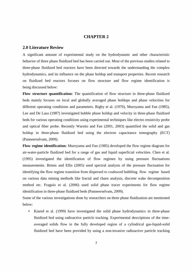
2.0 Literature Review
A significant amount of experimental study on the hydrodynamic and other characteristic
behavior of three phase fluidized bed has been carried out. Most of the previous studies related to
three-phase fluidized bed reactors have been directed towards the understanding the complex
hydrodynamics, and its influence on the phase holdup and transport properties. Recent research
on fluidized bed reactors focuses on flow structure and flow regime identification is
being discussed below:
Flow structure quantification: The quantification of flow structure in three-phase fluidized
beds mainly focuses on local and globally averaged phase holdups and phase velocities for
different operating conditions and parameters. Rigby et al. (1970), Muroyama and Fan (1985),
Lee and De Lasa (1987) investigated bubble phase holdup and velocity in three-phase fluidized
beds for various operating conditions using experimental techniques like electro resistivity probe
and optical fiber probe. Recently Warsito and Fan (2001, 2003) quantified the solid and gas
holdup in three-phase fluidized bed using the electron capacitance tomography (ECT)
(Panneerselvam, 2009).
Flow regime identification: Muroyama and Fan (1985) developed the flow regime diagram for
air-water-particle fluidized bed for a range of gas and liquid superficial velocities. Chen et al.
(1995) investigated the identification of flow regimes by using pressure fluctuations
measurements. Briens and Ellis (2005) used spectral analysis of the pressure fluctuation for
identifying the flow regime transition from dispersed to coalesced bubbling flow regime based
on various data mining methods like fractal and chaos analysis, discrete wake decomposition
method etc. Fraguío et al. (2006) used solid phase tracer experiments for flow regime
identification in three-phase fluidized beds (Panneerselvam, 2009).
Some of the various investigations done by researchers on three phase fluidization are mentioned
below:
• Kiared et al. (1999) have investigated the solid phase hydrodynamics in three-phase
fluidized bed using radioactive particle tracking. Experimental descriptions of the time-
averaged solids flow in the fully developed region of a cylindrical gas-liquid-solid
fluidized bed have been provided by using a non-invasive radioactive particle tracking

8
technique (RPT). The 3-D local instantaneous velocity components (radial, axial,
azimuthal) of a single radioactive solid tracer have been measured over extended time
period. Radial distributions of axial and radial mean turbulent velocities of particle, shear
stress and eddy diffusion coefficients have been established.
• Sokol and Halfani (1999) have studied the hydrodynamics of gas-liquid-solid fluidized
bed bioreactor with a low density biomass support (matrix density smaller than that of
water). It has been found that the air holdup increases with increase in the inlet air
velocity.
• Allia et al. (2006) have carried out the hydrodynamic study of three phase fluidized bed
bioreactors used for the removal of hydrocarbons from the refinery waste water. The
study allowed the determination of operating conditions before treatment experiments.
The obtained results have shown that in the three-phase fluidized bed the hydrocarbons
degrade more rapidly than in a closed aerated bioreactor.
Even though a large number of experimental studies have been directed towards the
quantification of flow structure and flow regime identification for different process parameters
and physical properties, the complex hydrodynamics of these reactors are not well understood
due to the interaction of all the three phases simultaneously. It has been a very tedious task to
analyze the hydrodynamic property in experimental way of three phase fluidized bed reactor, so
another advanced modeling approaches based on CFD techniques have been applied for
investigation of three phases for accurate design and scale up. Basically two approaches namely,
the Euler-Euler formulation based on the interpenetrating multi-fluid model, and the Euler-
Lagrangian approach based on solving Newton's equation of motion for the dispersed phase are
used.
2.2 Survey on CFD modeling
• Bahary et al. (1994) have used Eulerian multi-fluid approach for three-phase fluidized
bed, where gas phase treated as a particulate phase having 4 mm diameter and a kinetic
theory granular flow model applied for solid phase. They have simulated both symmetric
and axisymmetric model and verified the different flow regimes in the fluidized bed by
comparing with experimental data.
• Grevskott et al. (1996) have used Eulerian-Eulerian model approaches for three-phase
bubble column. The liquid phase along with the particles has been considered pseudo-

9
homogeneous by modifying the viscosity and density. The bubble size distribution based
on the bubble induced turbulent length and the local turbulent kinetic energy has been
studied. Variations of bubble size distribution, liquid circulation and solid movement
along radial direction have been discussed.
• Mitra-Majumdar et al. (1997) have taken multi-fluid Eulerian approach for three-phase
bubble column. They have used modified drag correlation between the liquid and the gas
phase to account for the effect of solid particles and between the solid and the liquid
phase to account for the effect of gas bubbles. A k-ε turbulence model has been used for
the turbulence and considered the effect of bubbles on liquid phase turbulence. Axial
variation of gas holdup and solid holdup profiles for various range of liquid and gas
superficial velocities and solid circulation velocity have been examined.
• Jianping and Shonglin (1998) have worked in 2-D with Eulerian-Eulerian method for k-
e–k-e three-phase bubble column for turbulence. Turbulence model and Pseudo-two-
phase fluid dynamic model have been used. The local axial liquid velocity and local gas
holdup with have been validated experimental data.
• Li et al. (1999) have studied in 2-D with Eulerian-Lagrangian model for three-phase
fluidization. The Eularian fluid dynamic method, the dispersed particle method (DPM)
and the volume-of-fluid (VOF) method have been used to account for the flow of liquid,
solid and gas phases respectively. A continuum surface force (CSF) model, a surface
tension force model and Newton's third law have been applied to account for the
interphase couplings of gas-liquid, particle-bubble and particle-liquid interactions
respectively. A close distance interaction (CDI) model included in the particle-particle
collision analysis, which considers the liquid interstitial effects between colliding
particles. Single bubble rising velocity in a liquid-solid fluidized bed and the bubble wake
structure and bubble rise velocity in liquid and liquid-solid medium have been
investigated.
• Padial et al. (2000) have worked in 3-D with multi-fluid Eulerian approach for three-
phase draft-tube bubble column. The drag force between solid particles and gas bubbles
has been modeled in the same way as that of drag force between liquid and gas bubbles.
The gas volume fraction and liquid circulation in draft tube bubble column have been
simulated.
10
• Joshi et al. (2001) have studied the bubble column reactors using Computational flow
modeling with Euler-Lagrange approach. Understanding of the drag force, virtual mass
force and lift force and mechanism of the energy transfer from gas to liquid phase have
been explained. By using phases flow pattern results the effort has been concentrated to
design cylindrical bubble column. The effects of the superficial gas velocity, column
diameter and bubble slip velocity on the flow pattern have been examined and compared
with experimental velocity profiles.
• Matonis et al. (2002) have worked in 3-D with multi-fluid Eulerian approach for slurry
bubble column and used the Kinetic theory granular flow (KTGF) model for describing
the particulate phase. The k–ε based turbulence model has been taken for liquid phase
turbulence and the analysis of the time averaged solid velocity, volume fraction profiles,
shear Reynolds stress have been done and compared with experimental data.
• Feng et al. (2005) have used 3-D, multi-fluid Eulerian approach for three-phase bubble
column. The liquid phase along with the solid phase considered as a pseudo-
homogeneous phase in view of the ultrafine nanoparticles. The interface force model of
drag, lift and virtual mass and k-ε model for turbulence have been taken. They compared
the local time averaged liquid velocity and gas holdup profiles along the radial position.
• Schallenberg et al. (2005) have used 3-D, multi-fluid Eulerian approach for three-phase
bubble column. Gas-liquid drag coefficient based on single bubble rise modified for the
effect of solid phase. Extended k-e turbulence model to account for bubble-induced
turbulence has been used and the interphase momentum between two dispersed phases
included. Local gas and solid holdup as well as liquid velocities have been validated with
experimental data.
• Zhang and Ahmadi (2005) have used 2-D, Eulerian-Lagrangian model for three-phase
slurry reactor where interactions between bubble-liquid and particle-liquid have been
included. Particle-particle and bubble-bubble interactions have been accounted for by the
hard sphere model approach. Bubble coalescence has also been included in the model.
Transient characteristics of gas, liquid and particle phase flows in terms of flowstructure,
effect of bubble size on variation of flow patterns and instantaneous velocities have been
studied.
11
• Panneerselvam et al. (2009) have worked in 3D, Eulerian multi-fluid approach for gas-
liquid-solid fluidized bed. Kinetic theory granular flow (KTGF) model for describing the
particulate phase and a k-ε based turbulence model for liquid phase turbulence have been
used. The interphase momentum between two dispersed phases has been included. Radial
distributions of axial and radial solid velocities, axial and radial solid turbulent velocities,
shear stress, axial bubble velocity, axial liquid velocity and averaged gas holdup and
various energy flows have been studied.
• O'Rourke et al. (2009) have used 3D, Eulerian finite difference approach for gas-liquid-
solid fluidized bed. The mathematical model using multiphase particle-in-cell (MP-PIC)
method has been used for calculating particle dynamics (collisional exchange) in the
Computational-particle fluid dynamics (CPFD). Mass averaged velocity of solid and
liquid, particle velocity fluctuation, collision time, and liquid droplet distribution have
been studied.
• Jena (2009) has used 2D, Eulerian-Eulerian granular multi-phase approach for gas-liquid-
solid fluidized bed. The validation of the proposed CFD model is done with the
experimental data for the solid phase, the liquid phase and for the gas phase
hydrodynamics. The hydrodynamic parameters studied are bed pressure drop, bed
expansion (bed voidage) and gas holdup.
• Chalermsinsuwan et al. (2011). Two- and three-dimensional CFD modeling of Geldart A
particles in a thin bubbling fluidized bed. The mathematical model based upon the kinetic
theory of granular flow with a modified interphase exchange coefficient was successfully
used to compute the system hydrodynamics of fluid catalytic cracking (FCC) particles in
a thin bubbling fluidized bed with 2-D and three-dimensional (3-D) computational
Domains. Comparison of turbulence and dispersion coefficients of gas.
• Nguyen et al. (2011). have worked in 2-D with Eulerian-Eulerian method for CFD
modelling of glass bead particles in a three-phase fluidized bed. The drag model used for
simulating is Gidaspow model.
• Kumar et al. (2011). Euler-Euler two-phase fluid model has been used to simulate two-
phase (air and water) transient up-flow in bubble column (15cm diameter). The
turbulence in the liquid phase is described using the standard k-ε model. Pseudo two
phase simulations have been used to model the three phase flow with low solid loadings.

12
CHAPTER 3
3.0 CFD Modeling of Three Phase Fluidized Bed
3.1 CFD (Computational Fluid Dynamics)
Computational Fluid Dynamics (CFD) is a computer based study-mathematical, computer made
related to the dynamics of everything that flows. CFD is one of the branches of Modeling and
Simulation, which can imitate a real situation by assuming a mathematical model. For this, it can
be considered basic equations, boundary conditions, and constitutive equations. It uses numerical
methods to solve the fundamental nonlinear differential equations that describe fluid flow (the
Navier-Stokes and allied equations) for predefined geometries and boundary conditions. It is the
science of predicting fluid flow, heat transfer, mass transfer, chemical reactions, and related
phenomena by solving the mathematical equations which govern these processes using a
numerical process.
3.2 Advantages of CFD
• CFD Saves Cost and Time: CFD is a very compelling, non-intrusive, virtual modeling
technique with powerful visualization capabilities. CFD costs much less than experiments
because physical modifications are not necessary.
• CFD is Reliable: The numerical schemes and methods upon which CFD is based are
improving rapidly, so CFD results are increasingly reliable. CFD is a dependable tool
for design and analyses.
• Speed: CFD simulations can be executed in a short period of time.
• Ability to simulate real conditions: Many flow and heat transfer processes cannot be
(easily) tested, e.g. hypersonic flow. CFD provides the ability to theoretically simulate
any physical condition.
• Ability to simulate ideal conditions: CFD allows great control over the physical
process, and provides the ability to isolate specific phenomena for study. Example: a heat
transfer process can be idealized with adiabatic, constant heat flux, or constant
temperature boundaries.
• Comprehensive information: Experiments only permit data to be extracted at a limited
number of locations in the system (e.g. pressure and temperature probes, heat flux
13
gauges, LDV, etc.).CFD allows the analyst to examine a large number of locations in the
region of interest, and yields a comprehensive set of flow parameters for examination.
3.3 Limitations of CFD
Physical models:
CFD solutions rely upon physical models of real world processes (e.g. turbulence,
compressibility, chemistry, multiphase flow, etc.). The CFD solutions can only be as accurate as
the physical models on which they are based.
Numerical errors:
Solving equations on a computer invariably introduces numerical errors.
• Round-off error: due to finite word size available on the computer. Round-off errors will
always exist (though they can be small in most cases).
• Truncation error: due to approximations in the numerical models. Truncation errors will
go to zero as the grid is refined. Mesh refinement is one way to deal with truncation error.
Boundary conditions:
As with physical models, the accuracy of the CFD solution is only as good as the
initial/boundary conditions provided to the numerical model. Example: flow in a duct with
sudden expansion. If flow is supplied to domain by a pipe, you should use a fully-developed
profile for velocity rather than assume uniform conditions.
3.4 Applications of CFD
Biomedical:
Flow modeling with computational fluid dynamics (CFD) software helps to visualize and predict
physical phenomena related to the flow of any substance. It is widely used in medical,
pharmaceutical and biomedical applications to analyze:
• manufacturing processes,
• device performance,
• physiological flows,
• fluid-structure interactions,
• The effectiveness of drug delivery systems, etc.

14
Industrial applications:
CFD is used in wide variety of disciplines and industries, including aerospace, automotive,
power generation, chemical manufacturing, polymer processing, petroleum exploration, pulp and
paper operation, medical research, meteorology, and astrophysics.
Environmental:
Protecting and improving the quality of our environment today requires innovative design
solutions that establish compliance with ever-expanding and more stringent regulations. Flow
modeling with Ansys’ computational fluid dynamics (CFD) software helps to tackle our
environmental flow problems in the most efficient and cost-effective way.
Civil:
Computational Fluid Dynamics (CFD) software is a powerful tool that allows us to create a
virtual airflow model of our building or urban environment to assess and optimize these factors
before construction commences. Modifications to an existing building can also be simulated
using CFD prior to any physical alterations. This approach helps to prevent costly mistakes and
minimize design risks while allowing innovation.
3.5 Working of CFD code
In order to provide easy access to their solving power all commercial CFD packages include
sophisticated user interfaces input problem parameters and to examine the results. Hence
allcodes contain three main elements (Bakker, 2002).
1. Pre-processing
2. Solver
3. Post –processing.

15
3.5.1 Pre-Processing
In Preprocessing, it consist of input of a flow problem by means of an operator friendly Interface
and subsequent transformation of this input into a suitable form which can be used by the solver.
This step is performed by software tool such as, GAMBIT, TGRID and DM (Design modular of
ANSYS). The Pre-processing stage involves the following steps (Bakker. 2002).
• Defining the geometry of the region for computational domain.
• Generating the Grids for subdivision of the domain into a number of smaller, non-over
lapping sub domains.
• Specifying the appropriate boundary and continuum conditions at cells, which coincide
with or touch the boundary.
The solution of a flow problem (Phase holdup, velocity, pressure, temperature etc.) is defined in
each cell in various nonlinear equations form. The accuracy of CFD solutions is governed by
number of cells in the grid. In general, the larger numbers of cells better the solution accuracy.
3.5.2 Solver
The CFD solver does the flow calculations and produces the desired results. ANSYS FLUENT
13 uses the finite-volume method to solve the governing equations for a fluid. It provides the
capability to use different physical models such as incompressible or compressible, in viscid or
viscous, laminar or turbulent, etc. Governing equations are non-linear and coupled, several
iterations of the solution loop are performed by solver before a converged solution is obtained
(Bakker., 2002) and the main functions of Solver are as follows:
• Approximation of unknown flow variables by means of simple functions.
• Discretization by substitution of the approximation into the governing flow equations and
subsequent mathematical manipulations.
• Solving the algebraic equations.

16
3.5.3 Post-Processing
This is the final step in CFD analysis, and it involves the results and interpretation of the
predicted flow data. ANSYS FLUENT 13 software includes full post processing capabilities and
exports CFD data to third-party post-processors and visualization tools such as Ensight, Field
view and Tech Plot (Bakker. 2002).
The main outcomes of post processing are -
• Domain geometry & Grid display.
• Contour plot of all the properties.
• Vector plots.
• Animations.
• 2D & 3D surface plots.
• X-Y plots with different properties.
• Particle tracking.
• Plot convergence.
• View manipulation (translation, rotation, scaling etc.)
3.6 Discretization Methods in CFD
There are three discretization methods in CFD:
1. Finite difference method (FDM)
2. Finite volume method (FVM)
3. Finite element method (FEM)
1. Finite difference method (FDM): A finite difference method (FDM) discretization is based
upon the differential form of the PDE to be solved. Each derivative is replaced with an
approximate difference formula (that can generally be derived from a Taylor series expansion).
The computational domain is usually divided into hexahedral cells (the grid), and the solution
will be obtained at each nodal point. The FDM is easiest to understand when the physical grid is
Cartesian, but through the use of curvilinear transforms the method can be extended to domains
that are not easily represented by brick-shaped elements. The discretization results in a system of
17
equation of the variable at nodal points, and once a solution is found, then we have a discrete
representation of the solution.
2. Finite volume method (FVM): A finite volume method (FVM) discretization is based upon
an integral form of the PDE to be solved (e.g. conservation of mass, momentum, or energy). The
PDE is written in a form which can be solved for a given finite volume (or cell). The
computational domain is discretized into finite volumes and then for every volume the governing
equations are solved. The resulting system of equations usually involves fluxes of the conserved
variable, and thus the calculation of fluxes is very important in FVM. The basic advantage of this
method over FDM is it does not require the use of structured grids, and the effort to convert the
given mesh in to structured numerical grid internally is completely avoided. As with FDM, the
resulting approximate solution is a discrete, but the variables are typically placed at cell centers
rather than at nodal points. This is not always true, as there are also face-centered finite volume
methods. In any case, the values of field variables at non-storage locations (e.g. vertices) are
obtained using interpolation.
3. Finite element method (FEM): A finite element method (FEM) discretization is based upon
a piecewise representation of the solution in terms of specified basis functions. The
computational domain is divided up into smaller domains (finite elements) and the solution in
each element is constructed from the basic functions. The actual equations that are solved are
typically obtained by restating the conservation equation in weak form: the field variables are
written in terms of the basic functions; the equation is multiplied by appropriate test functions,
and then integrated over an element. Since the FEM solution is in terms of specific basis
functions, a great deal more is known about the solution than for either FDM or FVM. This can
be a double-edged sword, as the choice of basic functions is very important and boundary
conditions may be more difficult to formulate. Again, a system of equations is obtained (usually
for nodal values) that must be solved to obtain a solution.
Comparison of the three methods is difficult, primarily due to the many variations of all three
methods. FVM and FDM provide discrete solutions, while FEM provides a continuous (up to a
point) solution. FVM and FDM are generally considered easier to program than FEM, but
opinions vary on this point. FVM are generally expected to provide better conservation
properties, but opinions vary on this point also.
18
3.7 Approaches to Multiphase Modeling
For a Multiphase flow there are two approaches for numerical calculations:
1. Euler-Lagrange approach
2. Euler-Euler approach
3.7.1 The Euler Lagrange Approach
This approach is applicable to continuous-dispersed systems and is often referred to as a discrete
particle model or particle transport model. The primary phase is continuous and is composed of a
gas or a liquid. The secondary phase is discrete and can be composed of particles, drops or
bubbles. In the Eulerian-Lagrangian (E–L) approach, the continuous phase is treated in an
Eulerian framework (using averaged equations). Its continuous-phase flow field is computed by
solving the Navier-Stokes equations. The dispersed phase is represented by tracking a small
number of representative particle streams. For each particle stream, ordinary differential
equations representing mass, momentum and energy transfer are solved to compute its state and
location. The two phases are coupled by inclusion of appropriate interaction terms in the
continuous-phase equations. In this approach the volume displaced by the dispersed phase is not
taken into account. So, this approach is applicable for low-volume fractions of the dispersed
phase. This approach is applicable for situations in which the discrete phase is injected as a
continuous stream into the continuous phase. A force balance equation based on Newton’s
second law of motion is solved to compute the trajectory of the discrete phase. Particle
trajectories are computed individually at specified intervals during the fluid phase calculations
and dispersed second phase occupies low volume fractions which are the fundamental
assumptions in this model.
The Eulerian-Lagrangian approach is suitable to unit operations in which the volume fraction of
the dispersed phase is small, such in spray dryers, coal and liquid fuel combustion, and some
particle-laden flow. This approach provides complete information on the behavior and residence
time of individual particles. Interaction of individual particle streams with turbulent eddied and
solid surfaces such as walls can be modeled.
3.7.2 The Euler-Euler Approach
Eulerian-Eulerian approach is the most general approach for solving multiphase flows. It is based
on the principle of interpenetrating continua, where each phase is governed by the Navier-Stokes
equations. The phases share the same volume and penetrate each other in space and exchange

19
mass, momentum and energy. Each phase is described by itsphysical properties and its own
velocity, pressure, concentration and temperature field. The interphase transfer between phases is
computed using empirical closure relations.
The Eulerian-Eulerian approach is applicable for continuous-dispersed and continuous-
continuous systems. For continuous-dispersed systems, the velocity of each phase is computed
using the Navier-Stokes equations. The dispersed phase can be in the form of particles, drops or
bubbles. The forces acting on the dispersed phase are modeled using empirical correlations and
are included as part of the interphase transfer terms. In addition, drag, lift, gravity, buoyancy and
virtual-mass effects are some of the forces that might be actingon the dispersed phase. These
forces are computed for an individual particle and thenscaled by the local volume fraction to
account for multiple particles.
In this approach the concept of volume fraction is introduced based upon the fact that the volume
of a phase cannot be carried or occupied by other phases. Here the different phases are treated
mathematically as interpenetrating continua. The volume fractions are assumed to be continuous
functions of space and time and their sum is equal to one. For each of the phase, conservation
equations are derived to obtain a set of equations which have similar structure for all phases
(Kumar, 2009).
The three different Euler-Euler Multiphase models available are
• The Volume of fluid (VOF) model
• The Mixture Model
• The Eulerian model
1. The VOF Model
In computational fluid dynamics, the Volume of fluid method is one of the most well known
methods for volume tracking and locating the free surface. The motion of all phases is modeled
by solving a single set of transport equations with appropriate jump boundary conditions at the
interface. The VOF model can model two or more immiscible fluids by solving a single set of
momentum equations and tracking the volume fraction of each of the fluids throughout the
domain. It is generally used to figure out a time dependent solution but for problems which are
concerned with steady state solution; it is possible to perform a steady state calculation. A steady
state VOF calculation is practical only when the solution is independent of the initial conditions
and there are distinct inflow boundaries for the individual phases (Heidari, 2007). Typical

20
applications include the motion of large bubbles in a liquid, the motion of liquid after a dam
break, the prediction of jet breakup, and the steady or transient tracking of any liquid-gas
interface. In general, the steady or transient VOF formulation relies on the fact that two or more
fluids (or phases) are not interpenetrating.
2. The Mixture Model
The mixture model is a simplified multiphase model that can be used to model multiphase flows
where the phases move at different velocities, but assume local equilibrium over short spatial
length scales. This model is designed for two or more phases (fluid or particulate). The mixture
model can apply to model multiphase flows where the different phases move at different
velocities and also it is applicable to model homogeneous multiphase flow and to calculate non-
Newtonian viscosity. The mixture model can model n phases (fluid or particulate) by solving
both the continuity equation and the momentum equation for the mixture, where mixture can be a
combination of continuous phase and the dispersed phase. In addition, the mixture model solves
the energy equation for the mixture and the volume fraction equation for the secondary phases,
as well as algebraic expressions for the relative velocities (if the phases are moving at different
velocities). Also it allows us to select the granular phases and we can calculate the different
properties for granular phases. It is applicable in the particle-laden flows with low loading, and
bubbly flows where the gas volume fraction remains low, cyclone separators, sedimentation and
in liquid-solid flows. It can also be used to model homogenous multiphase flows with very
strong coupling and the phases moving at the same velocity. It is a good substitute for the full
Eulerian multiphase model in several cases.
3. The Eulerian Model
The Eulerian model is the most complex among other multiphase models. It solves a set of n
momentum and continuity equations for each phase coupling is achieved through the pressure
and interphase exchange coefficients. The manner of handling of these couplings depends upon
the type of phases involved. Granular (fluid-solid) flows are handled differently than non
granular (fluid-fluid) flows. For granular flows, the properties are obtained by applying kinetic
theory.

21
3.8 Computational Flow Model
The simulation of three phase fluidized bed is performed by solving the governing equations of
mass and momentum conservation using fluent software. Eulerian multi-fluid model is adopted
in the present work where gas and liquid phases are all treated as continuous, inter-penetrating
and interacting everywhere within the computational domain. The pressure filed is assumed to be
shared by all the three phases proportional to their volume fraction. Here three dimensional (3D)
transient model is developed to simulate the gas hold up of a gas-liquid-solid fluidized bed using
the CFD method. The 3D geometry is considered with the quadrilateral-meshing scheme.
Continuity equation:
��������� + ∇������� = 0
Where �� is the density and �� is the volume fraction of phase � = gas, liquid, solid. The volume
fraction of the three phases satisfies the following condition.
� + �� + �� = 1
Momentum equations:
For liquid phase
��� ���. ��. �� + ∇. �������� = −��∇� + ∇. �� + ����� + ��,�
Liquid-solid interphase drag force:
The inter-phase exchange coefficient between the liquid and the solid phases, KLs is obtained by
Gidaspow drag model (1994) (it is combination of Wen and Yu model and the Ergun equation)
as:
� � = 150. ��2. � � ��
2 + 1.75��� | − �|� ��
, � ≤ 0.8
� � = 34 $%��� �
& − '�(��
)&� ( , � > 0.8

22
Where $% is the drag co-efficient proposed by wen and yu (1966) and is given as
$% = 24� +,�
&1 + 0.15 -� +,�(0.687/ +,� ≤ 1000
$% = 0.44 , +,� ≥ 1000
Gas-Liquid interphase drag force: The drag model of Schiller and Naumann (1935),
acceptable for general use for all fluid-fluid pairs of phases and is given by
) = $1+,24
Where $% = 24+,�
&1 + 0.15 -+,2(0.687/ , +,2 ≤ 1000
$% = 0.44 , +,2 ≥ 1000
3.9 Numerical Methodology
The CFD simulations were carried out for a fluidized bed having diameter 0.1 m and height 1.88
m. The working fluids were water and air. The working solid was spherical glass beads of
different diameter. The CFD simulations were performed using commercial CFD code ANSYS
FLUENT 13. The assumptions made for hydrodynamic modeling of three phase fluidized bed
are Transient as well as unsteady state, Isothermal flow conditions, so no energy equations, Mass
transfer and chemical reactions have been neglected, Liquid phase turbulence was modeled using
the k-ε model; the dispersed phases were considered laminar, The system of equations was
solved using a finite-volume scheme, Momentum transfer between the liquid and the dispersed
phases was modeled using the appropriate drag laws for the respective flow regime, Momentum
transfer between the dispersed phases was neglected, Bubbles are assumed as rigid sphere having
a constant diameter. The simulation of three phase fluidized bed was performed by solving the
governing equations of mass and momentum conservation using fluent software. Eulerian multi-
fluid model is adopted in the present work where gas and liquid phases are all treated as
continuous, inter-penetrating and interacting everywhere within the computational domain. The
pressure filed is assumed to be shared by all the three phases proportional to their volume
fraction. The motion of each phase is governed by the respective mass and momentum equations.
With the Eulerian multiphase model, the number of secondary phases is limited only by memory

23
requirements and convergence behavior. Any number of secondary phases can be modeled, if
sufficient memory is available.
3.9.1 Geometry and Mesh
ANSYS FLUENT 13 is used for making 3D rectangular geometry with width of 0.1m and height
1.88m.
Table 3.1 Mesh Information
Domain Node Element
Fluid 6095 4788
3.9.2 Selection of Models for Simulation
ANSYS FLUENT 13.0 is used for simulation. 3D segregated 1storder implicit unsteady solver is
used. Standard k-ɛ dispersed Eulerian multiphase model with standard wall functions were used
for modeling turbulence. The value of various model constants is tabulated as:
Model constants Value
Cmu 0.09
C1-Epsilon 1.44
C2-Epsilon 1.92

24
C3-Epsilon 1.3
TKE Prandtl Number 1
TDR Prandtl Number 1.3
Dispersion Prandtl Number 0.75
Water is taken as continuous phase while glass and air as dispersed phase. Inter-phase
interactions formulations used were
• Liquid – Air: Schiller-Naumann
• Solid-Liquid: Gidaspow
• Solid-Air:Gidaspow
Water velocities ranging from 0.2 to 0.16 m/s with increment of 0.02 and air velocities from
0.025 m/s to 0.0875 m/s are used respectively.
3.9.3 Solution
The Phase Coupled SIMPLE method (Patanker, 1980) has been chosen for pressure-velocity
coupling. The second-order upwind scheme has been used for discretization of momentum,
turbulence kinetic energy and turbulence dissipation rate and the first-order upwind scheme has
been used for discretization of volume-fraction equations. The time step size of 0.001s has been
used. The convergence criteria for all the numerical simulations are based on monitoring the
mass flow residual and the value of 1.0e–04 was set as converged value.
The following under relaxation factors have been used for different flow quantities: pressure =
0.5, density = 1, body forces = 1, momentum = 0.2, volume fraction = 0.5, granular temperature
= 0.2, turbulent kinetic energy = 0.8, turbulent dissipation rate = 0.8 and turbulent viscosity =1.
The simulations have been carried out till the system reached the quasi-steady state i.e., the
averaged flow variables are time independent; this can beachieved by monitoring the expanded
bed height or phase volume fractions.
RESULT AND DISCUSSION
A gas-liquid-solid fluidized bed of diameter 0.1m and height 1.88 m has been simulated using
commercial CFD software package FLUENT 13. Static bed of height 21.3 cm has been used for
simulation. Diameter of the glass beads (solid phase) are taken to be 2.18mm. Inlet superficial

25
velocities of gas are taken in a range of 0.025 m/s to 0.1 m/s while that of water is taken 0.02 m/s
to 0.16 m/s. The simulation results obtained have been shown in the figure 3.2.
Fig. 3.2 Contours of volume fraction of air at water velocity of 0.12 m/s and air velocity of
0.025 m/s for initial bed height of 21.3 cm.
While simulation takes place, a change in profile is seen in the column, but after some time no
significant change is observed which indicates that the quasi steady state has been reached.
Simulations are carried out till there is no change in the bed profile. From the figure it is very
much clear that the bed profile changes for the first 24 sec, after which there is no subsequent
change in the bed profile even though the simulation goes on, like that between 26 to 30 seconds.
3.10 Phase Dynamics
Solid, liquid and gas phase dynamics have been represented in the form of contours. Figure 3.3
shows the contours of volume fraction of solid, liquid and gas in the column obtained at water
velocity of 0.12m/s and air velocity of 0.025m/s for static bed height of 21.3 cm after the quasi
steady state is achieved. The colour scale given to the left of each contour indicates the value of

26
volume fraction corresponding to the colour. The contours for glass beads illustrates that bed is
in fluidized condition. The contour for water illustrates that volume fraction of the liquid is less
in fluidized section than the two-phase region above it. The contour for air illustrates that gas
holdup is significantly more in fluidized section of the bed compared to the two-phase region
above.
Fig. 3.3 Contours of volume fraction of solid, liquid and gas at water velocity of 0.12 m/s
and air velocity of 0.025 m/s for initial static bed height of 0.213 m.
3.11 Gas hold up
The gas holdup values are obtained from CFD simulation. Fig. 3.4 represents the variation of gas
holdup in the three-phase fluidized bed with superficial liquid velocity at constant gas velocity
for 2.18 mm glass beads at Hs= 0.213 m. The gas velocities taken are in the range from 0.025
m/s to 0.1 m/s and the liquid velocities taken are in the range from 0.02 m/s to 0.16 m/s. It is
seen from the figure that with increasing liquid velocity, the gas holdup decreases. The decrease
in gas holdup with liquid velocity may possibly be due to the fact that at higher liquid velocity

27
the bubbles are fast driven by the liquid. The residence time of the bubbles decreases with the
liquid velocity and hence the gas holdup is likely to decrease.
Fig. 3.4 Variation of gas holdup with liquid velocity at constant air velocity for 2.18 mm
glass beads at Hs= 0.213 m.
The Gas hold up values obtained from experiment,2D simulation (Jena,2009) and 3D simulation
in present study have been compared here. Fig. 3.5 shows a comparison of the gas holdup values
obtained from 3D simulation, 2D simulation and the experimental for air velocity 0.0625m for
initial bed height 21.3 cm.
0
0.02
0.04
0.06
0.08
0.1
0.12
0.14
0 0.05 0.1 0.15
Ga
s h
old
up
Superficial Liquid Velocity (m/s)
Ug=0.025 m/s
Ug=0.0375 m/s
Ug=0.05 m/s
Ug=0.0625 m/s
Ug=0.075 m/s
Ug=0.0875 m/s
Ug=0.01 m/s

28
Fig. 3.5 comparison of the gas holdup of air velocity 0.0625 m/s
Fig.3.6 represents the variation of fractional gas holdup with superficial gas velocity, at constant
liquid velocity for 2.18 mm glass beads at Hs=0.213 m. As seen from the figure, the fractional
gas holdup increases monotonically with the gas velocity having little higher value of the slope
at low gas velocities. In the lower range of gas velocity, an increase in gas velocity results in the
formation of a larger number of gas bubbles without appreciable increase in the bubble diameter.
Therefore an increasing fractional gas holdup is observed. As gas velocity increases, the bubble
size grows due to bubble coalescence and relatively the gas holdup decreases.
Fig. 3.6 Variation of gas holdup with gas velocity at constant liquid velocity for 2.18 mm
glass beads at Hs= 0.213 m.
0
0.02
0.04
0.06
0.08
0.1
0.12
0 0.05 0.1 0.15
Ga
s h
old
up
Superficial Liquid velocity (m/s)
3D simulation
2D simulation
(Jena,2009)
experimental
(Jena,2009)
0
0.02
0.04
0.06
0.08
0.1
0.12
0.14
0 0.02 0.04 0.06 0.08 0.1
Ga
s h
old
up
Superficial Gas velocity (m/s)
Ul=0.04 m/s
Ul=0.08 m/s
Ul=0.12 m/s
29
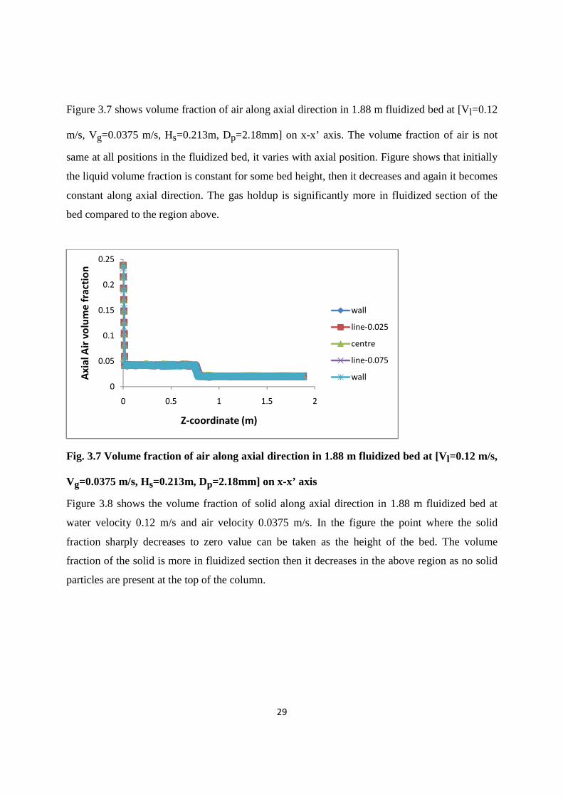
Figure 3.7 shows volume fraction of air along axial direction in 1.88 m fluidized bed at [Vl=0.12
m/s, Vg=0.0375 m/s, Hs=0.213m, Dp=2.18mm] on x-x’ axis. The volume fraction of air is not
same at all positions in the fluidized bed, it varies with axial position. Figure shows that initially
the liquid volume fraction is constant for some bed height, then it decreases and again it becomes
constant along axial direction. The gas holdup is significantly more in fluidized section of the
bed compared to the region above.
Fig. 3.7 Volume fraction of air along axial direction in 1.88 m fluidized bed at [Vl=0.12 m/s,
Vg=0.0375 m/s, Hs=0.213m, Dp=2.18mm] on x-x’ axis
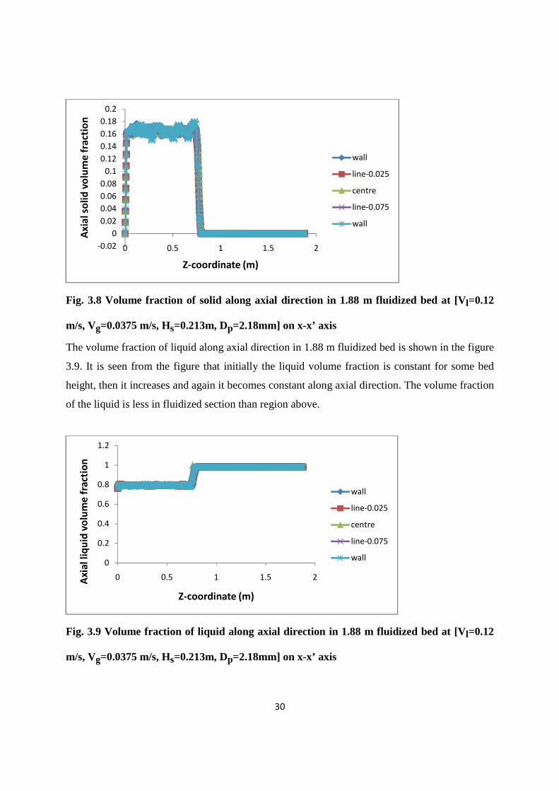
Figure 3.8 shows the volume fraction of solid along axial direction in 1.88 m fluidized bed at
water velocity 0.12 m/s and air velocity 0.0375 m/s. In the figure the point where the solid
fraction sharply decreases to zero value can be taken as the height of the bed. The volume
fraction of the solid is more in fluidized section then it decreases in the above region as no solid
particles are present at the top of the column.
0
0.05
0.1
0.15
0.2
0.25
0 0.5 1 1.5 2
Ax
ial
Air
vo
lum
e f
ract
ion
Z-coordinate (m)
wall
line-0.025
centre
line-0.075
wall
30
Fig. 3.8 Volume fraction of solid along axial direction in 1.88 m fluidized bed at [Vl=0.12
m/s, Vg=0.0375 m/s, Hs=0.213m, Dp=2.18mm] on x-x’ axis
The volume fraction of liquid along axial direction in 1.88 m fluidized bed is shown in the figure
3.9. It is seen from the figure that initially the liquid volume fraction is constant for some bed
height, then it increases and again it becomes constant along axial direction. The volume fraction
of the liquid is less in fluidized section than region above.
Fig. 3.9 Volume fraction of liquid along axial direction in 1.88 m fluidized bed at [Vl=0.12
m/s, Vg=0.0375 m/s, Hs=0.213m, Dp=2.18mm] on x-x’ axis
-0.02
0
0.02
0.04
0.06
0.08
0.1
0.12
0.14
0.16
0.18
0.2
0 0.5 1 1.5 2
Ax
ial
soli
d v
olu
me
fra
ctio
n
Z-coordinate (m)
wall
line-0.025
centre
line-0.075
wall
0
0.2
0.4
0.6
0.8
1
1.2
0 0.5 1 1.5 2Axi
al
liq
uid
vo
lum
e f
ract
ion
Z-coordinate (m)
wall
line-0.025
centre
line-0.075
wall

31
The volume fraction of gas, liquid and solid on y-y’ axis is similar as on x-x’ axis. Figure 3.10
shows the volume fraction of air along axial direction in 1.88 m fluidized bed at [Vl=0.12 m/s,
Vg=0.0375 m/s, Hs=0.213m, Dp=2.18mm on y-y’ axis. Figure shows that initially the liquid
volume fraction is constant for some bed height, then it decreases and again it becomes constant
along axial direction. The gas holdup is significantly more in fluidized section of the bed
compared to the region above.
Fig. 3.10 Volume fraction of air along axial direction in 1.88 m fluidized bed at [Vl=0.12
m/s, Vg=0.0375 m/s, Hs=0.213m, Dp=2.18mm] on y-y’ axis
Figure 3.11 shows the volume fraction of solid along axial direction in 1.88 m fluidized bed at
water velocity 0.12 m/s and air velocity 0.0375 m/s. In the figure the point where the solid
fraction sharply decreases to zero value can be taken as the height of the bed. The volume
fraction of the solid is more in fluidized section then it decreases in the above region as no solid
particles are present at the top of the column.
0
0.05
0.1
0.15
0.2
0.25
0 0.5 1 1.5 2
Axi
al
Air
vo
lum
e f
ract
ion
Z-coordinate (m)
wall
line-0.025
center
line-0.075
wall

32
Fig. 3.11 Volume fraction of solid along axial direction in 1.88 m fluidized bed at [Vl=0.12
m/s, Vg=0.0375 m/s, Hs=0.213m, Dp=2.18mm] on y-y’ axis
The volume fraction of liquid along axial direction in 1.88 m fluidized bed is shown in the figure
3.12. It is seen from the figure that initially the liquid volume fraction is constant for some bed
height, then it increases and again it becomes constant along axial direction. The volume fraction
of the liquid is less in fluidized section than region above.
Fig. 3.12 Volume fraction of liquid along axial direction in 1.88 m fluidized bed at [Vl=0.12
m/s, Vg=0.0375 m/s, Hs=0.213m, Dp=2.18mm] on y-y’ axis
-0.02
0
0.02
0.04
0.06
0.08
0.1
0.12
0.14
0.16
0.18
0.2
0 0.5 1 1.5 2
Ax
ial
soli
d v
olu
me
fra
ctio
n
Z-coordinate (m)
wall
line-0.025
center
line-0.075
wall
0
0.2
0.4
0.6
0.8
1
1.2
0 0.5 1 1.5 2Ax
ial
liq
uid
vo
lum
e f
ract
ion
Z-coordinate (m)
wall
line-0.025
center
line-0.075
wall

33
The volume fraction of glass bead shows the variation in volume fraction of glass bead along
radial direction at different bed heights on x-x’ axis. Figure 3.13 shows volume fraction of air
with different bed height along radial direction in 1.88 m fluidized bed at [Vl=0.12 m/s,
Vg=0.0375 m/s, Hs=0.213m, Dp=2.18mm]. It is seen from the figure that there is no subsequent
change in the volume fraction of air along radial direction. The maximum value of air volume
fraction is nearly 0.043 between bed heights 0.1 to 0.6 m. With further increase in bed height
there is a decrease in air volume fraction between 0.8 to 1.8 m the air volume fraction is 0.022.
Fig. 3.13 Volume fraction of air with different bed height along radial direction in 1.88 m
fluidized bed at [Vl=0.12 m/s, Vg=0.0375 m/s, Hs=0.213m, Dp=2.18mm] on x-x’ axis
Volume fraction of glass bead with different bed height along radial direction in 1.88 m fluidized
bed for air velocity of 0.0375 m/s and water velocity 0.12 m/s is shown in figure 3.14. It is seen
from the figure that there is no variation in solid volume fraction along the radius. This is
because the solid particles are uniformly distributed in the flow field with in the column. The
maximum value of air volume fraction is nearly 0.166 between bed heights 0.1 to 0.6 m. With
further increase in bed height volume fraction of glass bead decreases and finally reduces to zero
since no solid particles are there at the top of the column.
0
0.005
0.01
0.015
0.02
0.025
0.03
0.035
0.04
0.045
0.05
-0.06 -0.04 -0.02 0 0.02 0.04 0.06
Ra
dia
l a
ir v
olu
me
fra
ctio
n
X-coordinate (m)
line-0.1
line-0.2
line-0.3
line-0.4
line-0.5
line-0.6
line-0.7
line-0.8
line-0.9

34
Fig. 3.14 Volume fraction of solid with different bed height along radial direction in 1.88 m
fluidized bed at [Vl=0.12 m/s, Vg=0.0375 m/s, Hs=0.213m, Dp=2.18mm] on x-x’ axis
Figure 3.15 shows that there is no variation in volume fraction of liquid along the radius. The
maximum value of liquid volume fraction is 1 between bed heights 0.8 to 1.8 m. The liquid
volume fraction between 0.1 to 0.7 m is 0.8.
Fig. 3.15 Volume fraction of water with different bed height along radial direction in 1.88
m fluidized bed at [Vl=0.12 m/s, Vg=0.0375 m/s, Hs=0.213m, Dp=2.18mm] on x-x’ axis
-0.02
0
0.02
0.04
0.06
0.08
0.1
0.12
0.14
0.16
0.18
0.2
-0.06 -0.04 -0.02 0 0.02 0.04 0.06
Ra
dia
l so
lid
vo
lum
e f
ract
ion
X-coordinate (m)
line-0.1
line-0.2
line-0.3
line-0.4
line-0.5
line-0.6
line-0.7
line-0.8
line-0.9
line-1
0
0.2
0.4
0.6
0.8
1
1.2
-0.06 -0.04 -0.02 0 0.02 0.04 0.06
Ra
dia
l li
qu
id v
olu
me
fra
ctio
n
X-coordinate (m)
line-0.1
line-0.2
line-0.3
line-0.4
line-0.5
line-0.6
line-0.7
line-0.8
line-0.9
line-1
line-1.1

35
The magnitude of volume fraction of gas, liquid and solid on y-y’ axis are similar as on x-x’ axis.
Figure 3.16 shows volume fraction of air with different bed height along radial direction in 1.88
m fluidized bed at [Vl=0.12 m/s, Vg=0.0375 m/s, Hs=0.213m, Dp=2.18mm]. It is seen from the
figure that there is no subsequent change in the volume fraction of air along radial direction. The
maximum value of air volume fraction is nearly 0.043 between bed heights 0.1 to 0.6 m. With
further increase in bed height there is a decrease in air volume fraction between 0.8 to 1.8 m the
air volume fraction is 0.022.
Fig. 3.16 Volume fraction of air with different bed height along radial direction in 1.88 m
fluidized bed at [Vl=0.12 m/s, Vg=0.0375 m/s, Hs=0.213m, Dp=2.18mm] on y-y’ axis
Volume fraction of glass bead with different bed height along radial direction in 1.88 m fluidized
bed for air velocity of 0.0375 m/s and water velocity 0.12 m/s is shown in figure 3.17. It is seen
from the figure that there is no variation in solid volume fraction along the radius as solid
particles are uniformly distributed in the flow field with in the column. The maximum value of
air volume fraction is nearly 0.165 between bed heights 0.1 to 0.6 m. With further increase in
bed height volume fraction of glass bead decreases and finally reduces to zero since no solid
particles are there at the top of the column.
0
0.005
0.01
0.015
0.02
0.025
0.03
0.035
0.04
0.045
0.05
-0.06 -0.04 -0.02 0 0.02 0.04 0.06
Ra
dia
l a
ir v
olu
me
fra
ctio
n
Y-coordinate (m)
line-0.1
line-0.2
line-0.3
line-0.4
line-0.5
line-0.6
line-0.7
line-0.8
line-0.9
line-1

36
Fig. 3.17 Volume fraction of glass bead with different bed height along radial direction in
1.88 m fluidized bed at [Vl=0.12 m/s, Vg=0.0375 m/s, Hs=0.213m, Dp=2.18mm] on y-y’ axis
Figure 3.18 shows that there is no variation in volume fraction of liquid along the radius. The
maximum value of liquid volume fraction is 0.98 between bed heights 0.8 to 1.8 m. The liquid
volume fraction between 0.1 to 0.7 m is 0.8.
Fig. 3.18 Volume fraction of water with different bed height along radial direction in 1.88
m fluidized bed at [Vl=0.12 m/s, Vg=0.0375 m/s, Hs=0.213m, Dp=2.18mm] on y-y’ axis
-0.02
0
0.02
0.04
0.06
0.08
0.1
0.12
0.14
0.16
0.18
0.2
-0.06 -0.04 -0.02 0 0.02 0.04 0.06
Ra
dia
l so
lid
vo
lum
e f
ract
ion
Y-coordinate (m)
line-0.1
line-0.2
line-0.3
line-0.4
line-0.5
line-0.6
line-0.7
line-0.8
line-0.9
line-1
0
0.2
0.4
0.6
0.8
1
1.2
-0.06 -0.04 -0.02 0 0.02 0.04 0.06Ra
dia
l li
qu
id v
olu
me
fra
ctio
n
Y-coordinate (m)
line-0.1
line-0.2
line-0.3
line-0.4
line-0.5
line-0.6
line-0.7
line-0.8
line-0.9
line-1
37
3.12 Bed Expansion
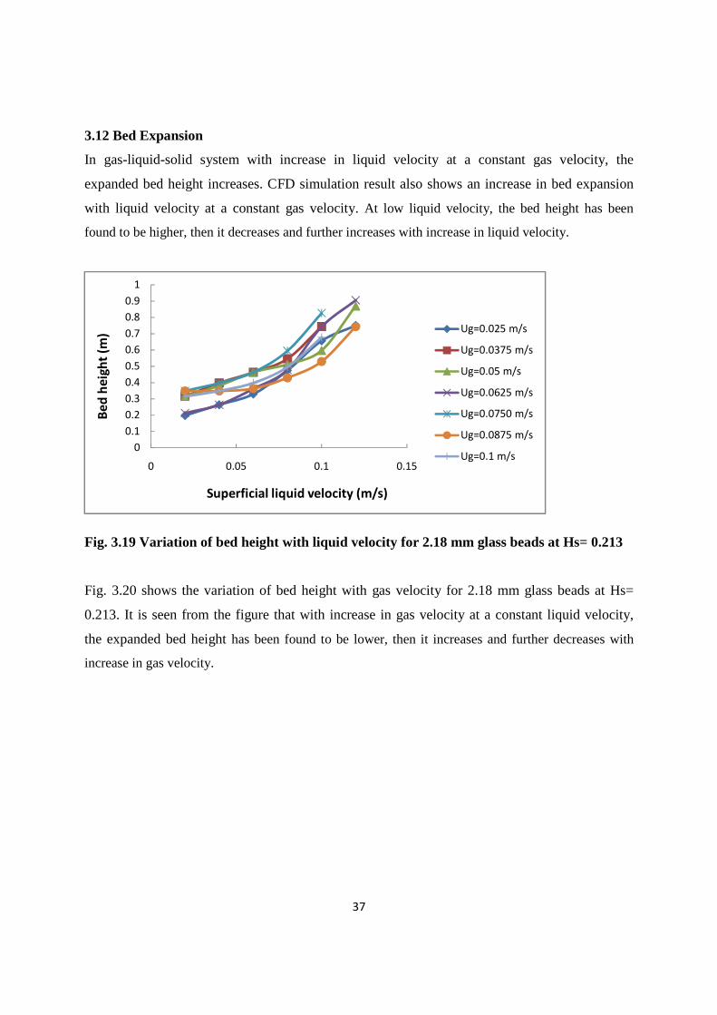
In gas-liquid-solid system with increase in liquid velocity at a constant gas velocity, the
expanded bed height increases. CFD simulation result also shows an increase in bed expansion
with liquid velocity at a constant gas velocity. At low liquid velocity, the bed height has been
found to be higher, then it decreases and further increases with increase in liquid velocity.
Fig. 3.19 Variation of bed height with liquid velocity for 2.18 mm glass beads at Hs= 0.213
Fig. 3.20 shows the variation of bed height with gas velocity for 2.18 mm glass beads at Hs=
0.213. It is seen from the figure that with increase in gas velocity at a constant liquid velocity,
the expanded bed height has been found to be lower, then it increases and further decreases with
increase in gas velocity.
0
0.1
0.2
0.3
0.4
0.5
0.6
0.7
0.8
0.9
1
0 0.05 0.1 0.15
Be
d h
eig
ht
(m)
Superficial liquid velocity (m/s)
Ug=0.025 m/s
Ug=0.0375 m/s
Ug=0.05 m/s
Ug=0.0625 m/s
Ug=0.0750 m/s
Ug=0.0875 m/s
Ug=0.1 m/s

38
Fig. 3.20 Variation of bed height with gas velocity for 2.18 mm glass beads at Hs= 0.213
0
0.1
0.2
0.3
0.4
0.5
0.6
0.7
0 0.02 0.04 0.06 0.08 0.1 0.12
Be
d h
eig
ht
(m)
Superficial gas velocity (m/s)
Ul-0.04
Ul-0.06
Ul-0.08
Ul-0.10

39
CHAPTER 4
4.0 CONCLUSION
CFD simulation of hydrodynamics of gas-liquid-solid fluidized bed has been carried out for
different operating conditions by employing the Eulerian-Eulerian granular multiphase approach.
The hydrodynamic parameters studied are gas hold up, bed expansion and operating variables
varied are gas and liquid velocity.
Main conclusions that can be drawn are:
• Gas holdup is more in fluidized part of the bed as illustrated by the contours for air.
• Contour of volume fraction of water shows that the volume fraction of water is less in
fluidized part of the column in comparison to the rest part.
• Bed expands when liquid velocity is increased at constant air velocity as illustrated from
the plot of bed expansion vs liquid velocity.
• With increase in gas velocity at a constant liquid velocity, the expanded bed height
initially increases and then decreases.
• Trends of gas holdup vs. inlet air velocity shows that gas holdup increases with increase
in air velocity obtained at constant water velocity.
• Trends of gas holdup vs. inlet Water velocity show that gas holdup decreases with the
increase in inlet water velocity at constant air velocity.
• Volume fraction of gas, liquid and solid with different bed height along radial direction
shows that there is no variation in the volume fractions along the radius.
40
REFERENCES
• Bahary, M., 1994. Experimental and computational studies of hydrodynamics in three-
phase and two-phase fluidized beds. Ph.D. Thesis, Illinois Institute of Technology,
Chicago.
• Bhatia, V.K., Epstein, N. 1974. Three Phase Fluidization: A Generalized Wake Model.
In: Fluidization and its Applications. H. Angelino et al., Eds., Cepadues Editions,
Toulouse, 380-392.
• Briens, L.A., Ellis, N., 2005. Hydrodynamics of three-phase fluidized bed systems
examined by statistical, fractal, chaos and wavelet analysis methods. Chemical
Engineering Science 60, 6094-6106.
• Chen, Z., Zheng, C., Feng, Y., 1995. Distributions of flow regimes and phase holdups in
three-phase fluidised beds. Chemical Engineering Science 50, 2153-2159.
• Chalermsinsuwan, B., Gidaspow, D., Piumsomboon, P., 2011. Two and three-
dimensional CFD modeling of Geldart A particles in a thin bubbling fluidised bed:
Comparison of turbulence and dispersion coefficients. Chemical Engineering Journal
171, 301-313.
• Epstein, N., 1981. Review: Three-Phase Fluidization-Some Knowledge Gaps. Canadian
Journal of Chemical Engineering 59, 649-757.
• Fan, L.S., 1989. Gas-Liquid-Solid Fluidization Engineering. Butterworth Series in
Chemical Engineering, Butterworth Publishers, Boston, MA.
• Fraguío, M.S., Cassanello, M.C., Larachi, F., Chaouki, J., 2006. Flow regime transition
pointers in three-phase fluidised beds inferred from a solid tracer trajectory. Chemical
Engineering and Processing 45, 350-358.
• Feng, W., Wen, J., Fan, J., Yuan, Q., Jia, X., Sun, Y., 2005. Local hydrodynamics of gas-
liquid-nano particles three-phase fluidization. Chemical Engineering Science 60, 6887-
6898.
• Grevskott, S., Sannaes, B.H., Dudukovic, M.P., Hjarbo, K.W., Svendsen, H.F., 1996.
Liquid circulation, bubble size distributions, and solids movement in two-and three-phase
bubble columns. Chemical Engineering Science51, 1703-1713.

41
• Jena, H.M., Sahoo, B.K., Roy, G.K., Meikap, B.C., 2008. Characterization of
hydrodynamic properties of a gas–liquid–solid three-phase fluidized bed with regular
shape spherical glass bead particles. Chemical Engineering Journal 145, 50-56.
• Jena H.M, 2009. Hydrodynamics of Gas-Liquid-Solid Fluidized and Semi-Fluidized
Beds. Ph.D. Thesis, National Institute of Technology, Rourkela.
• Jianping, W., Shonglin, X., 1998. Local hydrodynamics in a gas-liquid-solid three-phase
bubble column reactor. Chemical Engineering Journal 70, 81-84.
• Kiared, K., Larachi, F., Chaouki, J., Guy, C., 1999. Mean and turbulent particle velocity
in the fully developed region of a three-phase fluidised bed. Chemical Engineering &
Technology 22, 683-689.
• Kumar, S., Srinivasulu, N., Khanna, A., 2011. CFD Simulations to Validate Two &
Three Phase Up-flow in Bubble Columns. World Academy of Science, Engineering and
Technology 59,2223-2228.
• Lee, S.L.P., de Lasa, H.I., 1987. Phase holdups in three-phase fluidized beds. AIChE
Journal 33, 1359-1370.
• Li, Y., Zhang, J., Fan, L.S., 1999. Numerical simulation of gas-liquid-solid fluidization
systems using a combined CFD-VOF-DPM method: bubble wake behavior. Chemical
Engineering Science 54, 5101-5107.
• Matonis, D., Gidaspow, D., Bahary, M., 2002. CFD simulation of flow and turbulence in
a slurry bubble column. AIChE Journal 48, 1413–1429.
• Mitra-Majumdar, D., Farouk, B., Shah, Y.T., 1997. Hydrodynamic modeling of three-
phase flows through a vertical column. Chemical Engineering Science 52, 4485-4497.
• Muroyama, A., Fan, L.S., 1985. Fundamentals of gas–liquid–solid fluidization. A.I.Ch.E.
Journal 30, 1-34.
• Nguyen, K.T., Huang, S., 2011.Simulation of Hydrodynamic Characteristics of Glass
Beads in Gas-Liquid-Solid Three Phase Fluidized Beds by Computational Fluid
Dynamics. Journal of Engineering Technology and Education 8, 248-261.
• O'Rourke, P.J., Zhao, P.(P.), Snider, D., 2009. A model for collisional exchange in
gas/liquid/solid fluidized beds. Chemical Engineering Science 64, 1784-1797.
42
• Padial, N.T., Van der Heyden, W.B., Rauenzahn, R.M., Yarbro, S.L., 2000. Three
dimensional simulation of a three-phase draft-tube bubble column. Chemical Engineering
Science 55, 3261-3273.
• Panneerselvam, R., Savithri, S., Surender, G.D., 2009. CFD simulation of hydrodynamics
of gas–liquid–solid fluidised bed reactor. Chemical Engineering Science 64, 1119-1135.
• Rigby, G.R., Van Brokland, G.P., Park, W.H., Capes, C.E., 1970. Properties of bubbles in
three-phase fluidized bed as measured by an electroresistivity probe. Chemical
Engineering Science 25, 1729–1741.
• Safoniuk, M., Grace, J.R., Hackman, L., Mcknight, C.A., 2002. Gas Hold-Up in a Three-
Phase Fluidized Bed. AIChE Journal 48, 1581-1587.
• Schallenberg, J., En, J.H., Hempel, D.C., 2005. The important role of local dispersed
phase hold-ups for the calculation of three-phase bubble columns. Chemical Engineering
Science 60, 6027–6033.
• Sokol, W., Halfani, M.R., 1999. Hydrodynamics of a gas-liquid-solid fluidized bed
bioreactor with a low-density biomass support. Biochemical Engineering Journal 3, 185-
192.
• Warsito, W., Fan, L.S., 2001. Measurement of real-time flow structures in gas-liquid and
gas-liquid–solid flow systems using electrical capacitance tomography (ECT). Chemical
Engineering Science 56, 6455–6462.
• Zhang, X., Ahmadi, G., 2005. Eulerian-Lagrangian simulations of liquid-gas-solid flows
in three-phase slurry reactors. Chemical Engineering Science 60, 5089-5104.