pbh dark matter from axion in ation - arxiv.org e-print ... · a remarkable complementarity between...
TRANSCRIPT

PBH dark matter from axion inflation
Valerie Domcke1, Francesco Muia2, Mauro Pieroni3,
Lukas T. Witkowski4
1,3,4 AstroParticule et Cosmologie (APC)/Paris Centre for Cosmological Physics,
Universite Paris Diderot, CNRS, CEA, Observatoire de Paris, Sorbonne Paris Cite
University.2 Rudolf Peierls Centre for Theoretical Physics, University of Oxford,
1 Keble Road, Oxford OX1 3NP, UK.
Abstract
Protected by an approximate shift symmetry, axions are well motivated candidates
for driving cosmic inflation. Their generic coupling to the Chern-Simons term of any
gauge theory gives rise to a wide range of potentially observable signatures, including
equilateral non-Gaussianites in the CMB, chiral gravitational waves in the range of
direct gravitational wave detectors and primordial black holes (PBHs). In this paper
we revisit these predictions for axion inflation models non-minimally coupled to gravity.
Contrary to the case of minimally coupled models which typically predict scale-invariant
mass distributions for the generated PBHs at small scales, we demonstrate how broadly
peaked PBH spectra naturally arises in this setup. For specific parameter values, all of
dark matter can be accounted for by PBHs.
Dedicated to the memory of Pierre Binetruy
[email protected]@[email protected]@apc.univ-paris7.fr
arX
iv:1
704.
0346
4v2
[as
tro-
ph.C
O]
1 A
ug 2
017

Contents
1 Introduction 1
2 A review of axion inflation 4
2.1 Background dynamics . . . . . . . . . . . . . . . . . . . . . . . . . . . 4
2.2 Scalar and tensor power spectra . . . . . . . . . . . . . . . . . . . . . . 6
3 Non-minimal coupling to gravity 8
3.1 Background evolution . . . . . . . . . . . . . . . . . . . . . . . . . . . . 11
3.2 Perturbations . . . . . . . . . . . . . . . . . . . . . . . . . . . . . . . . 12
4 An example: attractor models 15
5 Primordial black holes 23
5.1 A quick review of PBH formation . . . . . . . . . . . . . . . . . . . . . 23
5.2 PBHs in models with non-minimal coupling to gravity . . . . . . . . . . 25
5.3 Searching for PBHs with GW interferometers . . . . . . . . . . . . . . 28
5.4 Discussion . . . . . . . . . . . . . . . . . . . . . . . . . . . . . . . . . . 30
6 Conclusion and Outlook 31
A Axions in field theory, supergravity and string theory 34
B Scalar power spectrum and consistency checks 41
C Uncertainties in the PBH production 43
1 Introduction
The recent detection of gravitational waves (GWs) emitted by a black hole (BH) binary
by the LIGO/VIRGO collaboration [1] marked not only the beginning of a new age of
GW astronomy but can also be seen as the first direct evidence of BHs. With a lot more
data from advanced LIGO/VIRGO and from the future space-mission LISA [2] on the
horizon, these are exciting times for considering possible implications for fundamental
physics and early universe cosmology.
1
Prompted by the LIGO discovery and the lack of positive results in dedicated dark
matter searches, the idea that primordial black holes (PBHs) could be (a fraction
of) dark matter has recently received a lot of attention [3–10]. PBHs are formed
when local over densities collapse due to their gravitational instability. Here we will
focus on the possibility that these local over densities are sourced by the primordial
scalar power spectrum of inflation (see e.g. Refs. [11, 12] for other recently discussed
possibilities). This requires an amplitude of the scalar power spectrum which is much
larger than the amplitude observed in the cosmic microwave background (CMB), i.e.
a highly blue spectrum. On the other hand, PBHs formed at very small scales are
strongly constrained by the traces their decays leave in the CMB and in the extra-
galactic gamma ray background [13]. A viable model of PBH dark matter thus requires
a non-trivial peaked structure of the primordial scalar power spectrum. It has been
demonstrated that such spectra can be achieved in multifield models of inflation [14–23]
or by arranging for the corresponding features in the scalar potential of inflation [24–26].
In this paper, we generate PBH dark matter in an inflation model which is based on two
simple, generic features: an axion-like inflaton with a non-minimal coupling to grav-
ity which increases towards the end of inflation. Axion-like particles are interesting
inflaton candidates for several reasons: (i) their approximate shift-symmetry protects
them from large mass contributions, preserving the required slow-roll phase of infla-
tion. (ii) they appear abundantly in supergravity as part of complex scalars as well
as in string theory [27], where they typically arise upon compactification of form field
gauge potentials. (iii) they generically couple to the topological Chern-Simons term
of any gauge group, leading to a wide range of potentially observable effects [28–31].
These include a non-Gaussian and blue contribution to the scalar spectrum, potentially
leading to PBH formation [26,32–36] as well as a blue, non-Gaussian and highly polar-
ized stochastic GW spectrum, potentially observable by LIGO or LISA [37–39]. The
predictions for different universality classes of pseudoscalar inflation have recently been
studied in Ref. [40]. Here we extend this work by allowing for a non-minimal coupling to
gravity, i.e. by considering simple Jordan frame inflation models. In recent years, such
a setup was found to be appealing both for deriving the supergravity Lagrangian [41]
and from a phenomenological perspective, driven most notably by the discussion of
Higgs inflation [42]. Such a non-minimal coupling to gravity is a characteristic feature
of supergravity in the Jordan frame [43–48]. The so-called attractor models at strong
coupling [44, 49] are an example of how the non-minimal coupling to gravity can be
2

used to construct classes of models which asymptote to the sweet spot of the Planck
data, see also [50–60] for other implementations.
Combining these two ingredients, the following picture emerges: at large scales (con-
strained by CMB observations [61]), i.e. early on in the inflationary epoch, both the
coupling to the Chern-Simons term and the non-minimal coupling to gravity are sup-
pressed. As inflation proceeds, the former generically induces a tachyonic instability in
the equation of motion for the gauge fields, leading to a gauge-field background which
in turn acts as an additional, classical source term for scalar and tensor perturbations.
This results in a strong increase of both spectra. Once the gauge field production has
reached a critical value, the back-reaction of the gauge fields on the inflaton dynam-
ics slows the growth of both spectra [31, 62, 63]. Finally, in the last stage of inflation
the non-minimal coupling to gravity becomes relevant and both the scalar and tensor
spectrum are suppressed. As a result, a significant fraction of dark matter (for spe-
cific parameter choices even all of dark matter) can be contained in PBHs. In part of
the parameter space their mergers may be observable by advanced LIGO. We observe
a remarkable complementarity between CMB observations, PBH constraints and GW
searches in constraining the parameter space of this setup.
The remainder of this paper is organized as follows. After a review of axion inflation
in Sec. 2, we extend the formalism to account for a non-minimal coupling to gravity in
Sec. 3. This in particular includes the computation of the resulting scalar and tensor
perturbations, sourced by both the quantum mechanical vacuum contribution and the
classical gauge field contribution. In Sec. 4 we apply these results to inflation models
described by attractors at strong coupling. We dedicate Sec. 5 to the production of
primordial black holes, discussing different regions of the parameter space based on a
handful of benchmark models. We conclude in Sec. 6. The main results of this paper
are supported by three appendices. In App. A we discuss how the type of axions we
consider here arise in the context of field theory, supergravity and string theory. Some
of the details of the derivations of the scalar power spectrum are left to App. B. Finally,
App. C analyses how uncertainties related to the PBH formation and evolution impact
our results.
3

2 A review of axion inflation
In this section we give a review5 of the case of a pseudoscalar inflaton φ coupled to
Abelian gauge fields. In particular we show that a generic higher-dimensional cou-
pling between the inflaton and the gauge fields introduces an instability in the theory,
which leads to an exponential production of the gauge fields [28–30]. Interestingly
this effect induces a back-reaction both on the background dynamics [31, 62, 63] and
on the perturbations [33, 38], leading to a wide set of observational consequences. Let
us consider the action for a pseudo-scalar inflaton φ, which is coupled to a certain
number N of Abelian gauge fields Aaµ (associated to U(1) gauge symmetries,6 i.e.
a = 1, 2, ...,N) [28–31,33,38,40,62,63]:7
S =
∫d4x√|g|[m2p
R
2− 1
2∂µφ ∂
µφ− V (φ)− 1
4F aµνF
µνa −
αa
4ΛφF a
µνFµνa
], (2.1)
where V (φ) is the inflaton potential, F aµν (F µν
a ) are the (dual8) field-strength tensors for
the gauge fields, Λ is a mass scale (that suppresses the higher-dimensional scalar-vector
coupling) and αa are the dimensionless coupling constants of the Abelian gauge fields.
In the following we consider αa = α for all a. Throughout this paper, the effective
mass scale Λ/α will take sub-Planckian values, as required for a reasonable effective
field theory. Typical values found e.g. in Ref. [40] for phenomenologically interesting
scenarios lie in the range Λ/α ' 0.01 − 0.03mp. However, we stress that contrary to
natural inflation models [64], we do not impose that this scale simultaneously sets the
scale of the scalar potential or of the field excursion during inflation. A discussion on
how Eq. (2.1) may arise in the context of field theory, supergravity or string theory is
provided in App. A.
2.1 Background dynamics
In order to describe the dynamics we can start by computing the background equations
of motion for the inflaton φ(t) and for the gauge fields Aaµ(t, x). Without loss of gen-
erality, we proceed by assuming φ > 0, V,φ(φ) > 0, φ < 0, and we choose to describe
5For more details see for example [31,33,63].6Alternatively, these may be associated with a SU(N ) symmetry in the weak coupling limit.7The metric has signature (−,+,+,+) and mp ' 2.4 · 1018 GeV denotes the reduced Planck mass.8The dual field-strength tensor is defined as Fµνa ≡ F aρσε
µνρσ/(2√−g), where εµνρσ is the Levi-
Civita tensor.
4

the problem in the Coulomb gauge (Aa0 = 0, ∂µAaµ(t, x) = 0). Under these assumptions
the equations of motion can be expressed as:
φ+ 3Hφ+∂V
∂φ=
α
2Λ
εµνρσ√|g|〈∂µAν∂ρAσ〉 ≡
α
Λ〈 ~Ea · ~Ba〉 , (2.2)
d2
dτ 2~Aa − ~∇2 ~Aa − α
Λ
dφ
dτ~∇× ~Aa = 0 , (2.3)
where dots are used to denote derivatives with respect to cosmic time t, primes are
used to denote derivatives with respect to τ (conformal time defined as dt ≡ a dτ), ~∇ is
the 3-dimensional flat space gradient operator, the brackets 〈·〉 denote a spatial mean
and the vectors ~Ea and ~Ba are the “electric” and “magnetic” fields associated with the
fields Aaµ(t, x) defined as:
~Ea ≡ − 1
a2
d ~Aa
dτ= −1
a
d ~Aa
dt, ~Ba ≡ 1
a2~∇× ~Aa . (2.4)
In order to completely specify the dynamics we also have to compute the Friedmann
equation which can be expressed as:
3H2m2p =
1
2φ2 + V (φ) +
1
2〈 ~Ea 2 + ~Ba 2〉 . (2.5)
Clearly a general analytical solution for Eq. (2.2), Eq. (2.3), and Eq. (2.5) does not exist.
However, assuming φ to be slowly varying (which is a reasonable assumption during
slow-roll inflation) we can find an analytical solution for Eq. (2.3). By substituting
this solution into Eq. (2.2) and Eq. (2.5) we can then study the back-reaction on the
system.
In order to solve Eq. (2.3) we start by performing a spatial Fourier transform and,
taking ~k to be parallel to the x-axis x, expressing the gauge fields in terms of the two
helicity vectors9 as ~Aa = Aa+~e+ + Aa−~e−, the equation of motion for the gauge fields
reads:d2Aa±(τ,~k)
dτ 2+
[k2 ± 2 k
ξ
τ
]Aa±(τ,~k) = 0 , (2.6)
where we have introduced the parameter ξ defined as:
ξ ≡ α |φ|2 ΛH
. (2.7)
9The two helicity vectors ~e± are defined as ~e± = (y± iz)/√
2. It is crucial to notice that using the
helicity vectors we get ~k × ~Aa = Aa±~k × ~e± = ∓iAa±|~k|~e±.
5

Notice that Eq. (2.6) describes a tachyonic instability for the A+ mode. In particular
for the modes with (8 ξ)−1 . k/(aH) . 2 ξ, A+ can be expressed as [32,62,63]:
Aa+ '1√2 k
(k
2 ξ aH
)1/4
eπξ−2√
2ξk/(aH) , (2.8)
so that the terms 〈 ~Ea · ~Ba〉 and 〈 ~Ea 2 + ~Ba 2〉 appearing in Eq. (2.2) and in Eq. (2.5)
can be expressed as:10
〈 ~Ea · ~Ba〉 ' N · 2.4 · 10−4H4
ξ4e2πξ ,
1
2〈 ~Ea 2 + ~Ba 2〉 ' N · 1.4 · 10−4H
4
ξ3e2πξ . (2.9)
It is possible to show (see for example [63]) that while the back-reaction on the Fried-
mann equation is fairly negligible throughout the whole evolution, the back-reaction
on the equation of motion for the scalar field cannot be neglected in the last part of
the evolution. In particular this back-reaction introduces an additional friction term
that has an exponential dependence on ξ. As this parameter is proportional to φ, it
typically increases towards the end of inflation in single-field inflation models. Corre-
spondingly the new friction term may be negligible at CMB scales while significantly
slowing down the last part of the evolution. As explained in [40], this effect induces a
shift in the region of the potential that can be probed with CMB observations. It is
crucial to stress that the gauge fields are not changing the total number N ≡ −∫Hdt
of e-foldings (i.e. the CMB is still generated at NCMB ' 60 in the complete evolution)
but rather they slow down the increase of ξ ∼ |φ/H|.
2.2 Scalar and tensor power spectra
The gauge fields do not only affect the background dynamics but they also modify
the equation of motion for the perturbations. In particular they induce a source term
both for scalar and tensor perturbations leading to an exponential amplification of the
spectra at small scales.
Let us start by discussing the modified scalar power spectrum.11 As a first step we
express the inflaton field as φ(~x, t) = φ(t) + δφ(~x, t) and by solving the linearized
equation of motion for δφ(~x, t) (for details see [30–32,62,63]) we can express the scalar
10These expressions only hold for ξ & 1. For the correct expressions for small values of ξ see [62,65].11More details on the derivation of these formulas are given in Sec. 3, where we also discuss the
generalization to a model where the inflaton is non-minimally coupled to gravity.
6

power spectrum ∆2s(k) as [33,40]:
∆2s(k) = ∆2
s(k)vac + ∆2s(k)gauge =
(H2
2π|φ|
)2
+
(α〈 ~Ea · ~Ba〉/
√N
3ΛbHφ
)2
, (2.10)
where we have defined b as:
b ≡ 1− 2 π ξα〈 ~Ea · ~Ba〉
3ΛHφ. (2.11)
As 〈 ~Ea · ~Ba〉 grows exponentially with ξ, the second term of Eq. (2.10) (i.e. the gauge-
field induced contribution) is typically negligible at CMB scales (where the stringent
CMB constraints essentially require ∆2s(k) ' ∆2
s(k)vac) but may dominate over the
first term at small scales. In particular it is possible to show that in the gauge-field
dominated regime (i.e. typically in the last part of inflation) the spectrum is well ap-
proximated by [33,40]:
∆2s(k) ' 1
N (2πξ)2. (2.12)
Notice that in presence of several U(1)s the power spectrum is suppressed at small
scales. Moreover, the presence of the gauge fields leads to the generation of equilateral
non-Gaussianities [38]. As a consequence, the non-observation of non-Gaussianities at
CMB scales [61, 66] can be used to set constraints on these models. In particular, this
implies ξ|CMB . 2.5, where ξ|CMB is the value of ξ at CMB scales [31–33,38,63].
In order to compute the tensor spectrum ∆2t we start with the equation of motion for
the traceless transverse part of the metric perturbations hij(~x, t), given by the linearized
Einstein equation:12
d2hijdτ 2
+ 2d ln a
dτ
dhijdτ− ~∇2hij =
2
m2p
Πµνij Tµν , (2.13)
where Πijµν is the transverse, traceless projector and Tµν is the matter energy-momentum
tensor (which acts as a source for GWs). By solving this equation we obtain ∆2t,L and
∆2t,R, power spectra for the two polarizations13 (L,R) of the GWs. The tensor power
spectrum ∆2t (given by the sum of the spectra for the two polarizations) can then be
expressed as:
ΩGW ≡ΩR,0
24∆2t '
1
12ΩR,0
(H
πmp
)2(1 + 4.3 · 10−7N H2
m2p ξ
6e4πξ
), (2.14)
12For details on the derivation of this equation see [67].13In order to decompose hij(~x, t) in terms of the two polarizations of the GW we can use the
projector Πij,L/R = ei,∓ej,∓.
7

where ΩR,0 = 8.6 · 10−5 is used to denote the radiation energy density today. Similarly
to the case of the scalar power spectrum, the gauge-field sourced term (i.e. the second
term in the parenthesis on the r.h.s. of Eq. (2.14)) is typically negligible at CMB scales
and dominates over the first term at small scales (i.e. in the last part of inflation). It
is also crucial to stress that the second term in Eq. (2.14) is only sourced by one of the
two polarizations. As a consequence the GW signal that is generated during the last
part of the evolution is expected to be strongly chiral. Chirality is a peculiar feature for
a GW background and if detected14 it would point to the existence of a parity violating
source. In the framework of standard general relativity axion inflation is one of the
simplest models which implement this parity violation.
As in the context of direct GW observations it is customary to express quantities in
terms of the frequency f = k/(2π), it is useful to introduce the relation between f and
the number of e-foldings N [31, 40]:
N = NCMB + lnkCMB
0.002 Mpc−1 − 44.9− lnf
102 Hz, (2.15)
where kCMB = 0.002 Mpc−1 and NCMB ' 50 − 60. Following the convention used
throughout this work, the number of e-foldings N decreases during inflation, reaching
N = 0 at the end of inflation and we will set NCMB = 60.
3 Non-minimal coupling to gravity
In this section15 we generalize the analysis presented in Sec. 2 to the case where the
inflaton is non-minimally coupled to gravity. In general non-minimal couplings between
the inflaton and gravity may naturally arise in the context of supergravity and string
theory [41] or from radiative corrections in the framework of QFT in curved space-
time.16 Moreover, during the last years it was realized that the introduction of a non-
minimal coupling between the inflaton and gravity (in the Jordan frame) can provide a
mechanism to “flatten” the inflationary potential (in the Einstein frame) [42,44,50–59,
70] leading to predictions for the scalar spectral index ns and the tensor-to-scalar-ratio
r that lie right in the sweet spot of the constraints set by CMB observations [61]. For
14For details on methods to detect the chirality of GW background see [68].15To ease the notation, in Secs. 3 and 4 we will work in Planck units, mp = 1, while reintroducing
mp in Sec. 5.16For an introduction to the topic see for example [69].
8

these reasons it is interesting to consider a generalization of the mechanism discussed
in Sec. 2 in order to take these models into account.
We start by considering the action for a pseudoscalar field φ non-minimally coupled to
gravity and coupled to an Abelian gauge field17 through the topological Chern-Simons
term,
S =
∫d4x√−gJ
[Ω(φ)R
2−X − VJ −
gµρJ gνσJ
4FµνFρσ −
α
8Λ
εµνρσ√−gJ
φFµνFρσ
], (3.1)
where εµνρσ is the Levi-Civita symbol, X ≡ gµνJ ∂µφ∂νφ/2, Fµν ≡ ∂µAν − ∂νAµ, α is the
coupling between the pseudoscalar and the gauge field, Λ is a mass scale that suppresses
the higher dimensional operator φFF and Ω(φ) is function of φ that without loss of
generality can be expressed as:
Ω(φ) = 1 + ςf(φ) , (3.2)
where ς is a the dimensionless coupling constant and f(φ) is a generic function of φ.
The case discussed in Sec. 2 can be easily recovered by setting ς = 0.
The action of Eq. (3.1) corresponds to a Jordan frame formulation of the theory (ex-
plaining the subscript J). The Einstein frame formulation (where gravity is described
by a standard Einstein-Hilbert term) of the theory is found via a conformal transfor-
mation:
gJ µν → gµν = Ω(φ)gJ µν , (3.3)
so that the action reads:
S =
∫d4x√−g[R
2−K(φ)X − VE −
gµρgνσ
4FµνFρσ −
α
4Λ
εµνρσ
2√−g
φFµνFρσ
], (3.4)
where VE ≡ VJ/Ω2(φ) and K(φ) is defined as:18
K(φ) ≡ Ω−1 +3
2
(d ln Ω
dφ
)2
. (3.5)
Note that the action shown in Eq. (3.4) is the action for a pseudoscalar field that
is minimally coupled to gravity but that has a non-standard kinetic term.19 As a
17The generalization to N Abelian gauge fields Aaµ is straight-forward. To ease the notation, we will
work with N = 1 here and re-introduce the parameter N only in the final expressions.18In order to make expressions simpler sometimes we will write K instead of K(φ).19Pseudoscalar theories from string theory compactifications typically exhibit a canonically coupling
to gravity, a coupling of the pseudoscalar to the topological term of a gauge theory as well as a non-
canonical kinetic term for the pseudoscalar. It is hence in the formulation in Eq. (3.4) that our model
may arise from string theory. For more details see appendix A.
9
consequence the treatment carried out in the rest of this section is valid for both these
cases.
In the following we discuss the evolution of the system defined by the action of Eq. (3.4).
In particular we study both the evolution of the homogeneous background and of per-
turbations around this background. As a first step we start by computing the equation
of motion for the gauge field. For this purpose we take the variation of the action
(expressed in terms of conformal coordinates) with respect to Aν :
δSδAν
= ∂µ
[ηµρηνσ
2(∂ρAσ − ∂σAρ)
]+
α
4Λ∂µ [φ εµνρσ (∂ρAσ − ∂σAρ)] = 0 , (3.6)
where ηµν is the Minkowski metric. At this point we can proceed by fixing the gauge. A
convenient gauge to describe the problem is Coulomb gauge, i.e. gµν∂µAν = 0, A0 = 0
so that the equation of motion reads:
ηνσ2Aσ −α
Λφ′ε0νρσ∂ρAσ = 0 , (3.7)
where 2 is the standard flat space d’Alembert operator 2 ≡ ηµν∂µ∂ν . As a consequence
we can write:
2 ~A− α
Λφ′ ~∇× ~A = 0 , (3.8)
where ~∇× is the usual curl operator and a prime is used to denote a derivative with
respect to τ . This equation matches with the Eq. (2.3) and thus the solution for the
gauge fields is exactly the same as in the case of a minimal coupling to gravity.
We can now consider the variation of the action (again in conformal time) with respect
to φ to get the equation of motion for the inflaton:
∂µ(ηµνK(φ)a2 ∂νφ
)− a4
(∂VE∂φ
(φ) +α
4ΛF µνF µν
)= 0 , (3.9)
which can be expressed as:
−K(φ)2φ− K,φ(φ)
2ηµν ∂µ φ∂νφ+ 2aHK(φ)φ′ + a2 VE,φ(φ) + a2α
Λ〈 ~E · ~B〉 = 0 , (3.10)
where ,φ is used to denote a derivative with respect to φ, primes are used to denote a
derivatives with respect to τ and H ≡ a′/a. At this point we can express φ as:
φ(τ, ~x) = φ0(τ) + δφ(τ, ~x) , (3.11)
where φ0(τ) is the (homogeneous) background solution and δφ(τ, ~x) is a small pertur-
bation. By substituting this parametrization into Eq. (3.10) it is easy to show that the
10

equation of motion for the background field φ0 reads:
K(φ0)φ′′0 +K,φ(φ0)
2φ′ 20 + 2aHK(φ0)φ′0 + a2 VE,φ(φ0) + a2α
Λ〈 ~E · ~B〉 = 0 . (3.12)
Conversely, the linearized equation of motion for the perturbation reads:
δφ′′ − ~∇2δφ+1
2
d
dφ
(d lnK
dφ
)φ′ 20 δφ+
d lnK
dφφ′0δφ
′ + 2aHδφ′+
+ a2 d
dφ
(VE,φK
)δφ− a2
K2K,φ
α
Λ〈 ~E · ~B〉δφ+
a2
K
α
Λδ(〈 ~E · ~B〉
)= 0 .
(3.13)
A detailed analysis on the evolution of the background and of the inflaton perturbation
is presented in Sec. 3.1 and in Sec. 3.2 respectively.
3.1 Background evolution
As a first step we express Eq. (3.12) in terms of cosmic time (dt = a dτ) and we divide
by K(φ0) to get:
φ0 +1
2
d lnK
dφ0
φ20 + 3Hφ0 +
VE,φ0K
+α
ΛK〈 ~E · ~B〉 = 0 . (3.14)
We can also express Friedmann equation as:
3H2 = Kφ2
0
2+ VE +
1
2〈 ~E2 + ~B2〉 . (3.15)
At this point we can solve Eq. (3.8) and plug the solution into Eq. (3.14) and Eq. (3.15)
to get:20
φ0 +1
2
d lnK
dφ0
φ20 + 3Hφ0 +
VE,φ0K− 2.4 · 10−4 α
ΛK
H4
ξ4e2πξ = 0 , (3.16)
3H2 = Kφ2
0
2+ VE + 1.4 · 10−4H
4
ξ3e2πξ , (3.17)
with the parameter ξ defined as in Eq. (2.7),
ξ ≡ α
2Λ
|φ0|H
. (3.18)
20Notice that these expressions for 〈 ~E · ~B〉 and 〈 ~E2 + ~B2〉 only hold for sizable values for ξ (i.e. for
ξ & 1). Different expressions should be used for small values of ξ, see [62].
11
Note that here φ0 is not the canonically normalized field. If the field φ0 is slow-rolling
these equations can be approximated as:
3Hφ0 +VE,φ0K− 2.4 · 10−4 α
ΛK
H4
ξ4e2πξ ' 0 , (3.19)
3H2 ' VE + 1.4 · 10−4H4
ξ3e2πξ , (3.20)
so that in the first part of the evolution (where ξ ' 1) we recover the usual slow-roll
equations:
φ0 ' −VE,φ03HK
, 3H2 ' VE . (3.21)
As in Sec. 2, the back-reaction of the gauge fields on the Friedmann equation (i.e.
Eq. (3.20)) is negligible throughout the whole evolution, but it may have a significant
impact on Eq. (3.19). As above, the 〈 ~E · ~B〉 term plays the role of a friction term which
grows exponentially with ξ. Notice that as long as the gauge field contribution is not
too strong we find for the first slow-roll parameter εH ,21
εH ≡ −H
H2' 1
2K(φ0)
(φ0
H
)2
∝ K(φ0)ξ2 , (3.22)
where we have used Eq. (3.21) and Eq. (3.18). As for a vast majority of slow-roll
inflationary models εH grows during inflation,22 for sufficiently large values of α/Λ we
expect a strong gauge field production that strongly affects the dynamics towards the
end of inflation. However, it is crucial to stress that in general ξ is not monotonically
increasing for all the slow-roll inflationary models. For example, if both εH and K(φ0)
monotonically increase during inflation, their interplay may lead to a local maximum
in ξ, if the growth in K(φ0) dominates the growth of εH at late times. Such a scenario
will be particularly relevant for the discussion of PBHs in Sec. 5.
3.2 Perturbations
In order to study the evolution of the inflaton perturbations we start by expressing the
δ(〈 ~E · ~B〉
)term appearing in Eq. (3.13) in a convenient form. In particular following
the treatment of [62] we proceed by using:
δ(〈 ~E · ~B〉
)= [ ~E · ~B−〈 ~E · ~B〉]δφ=0 +
∂〈 ~E · ~B〉∂φ0
δφ′
a≡ δ ~E· ~B −
( παΛH
)〈 ~E · ~B〉 δφ
′
a. (3.23)
21As long as the back-reaction of the gauge fields is negligible, this definition is equivalent to the
more commonly used ‘potential’ slow-roll parameter, εH ' εV = m2p(V
′(φ)/V )2/(2K).22In particular this happens for all the models considered in Sec. 4 (see Fig. 4.1).
12
We can thus proceed by substituting this expression into Eq. (3.13) (expressed in terms
of cosmic time) to get:
δφ−~∇2
a2δφ+
1
2
d
dφ0
(d lnK
dφ0
)φ2
0δφ+d lnK
dφ0
φ0˙δφ+ 3H ˙δφ+
d
dφ0
(VE,φ0K
)δφ
− 1
K
d lnK
dφ0
α
Λ〈 ~E · ~B〉δφ+
1
K
α
Λ
[δ ~E· ~B −
( παΛH
)〈 ~E · ~B〉 ˙δφ
]= 0 .
(3.24)
Let us start by discussing the regime where the gauge field contribution is negligible
before we proceed by considering the strong gauge field regime. If the gauge field con-
tribution is negligible the scalar power spectrum ∆2s(k) is simply given by the standard
vacuum amplitude:
∆2s(k)
∣∣vac' 1
8π2
H2
cs εH, (3.25)
where εH is the first (Hubble) slow-roll parameter defined in Eq. (3.22) and cs is the
speed of sound that for all the models considered in this work is equal to one. Using
Eq. (3.21) it is easy to show that the vacuum amplitude can be expressed as
∆2s(k)
∣∣vac' KV
12 π2
(d lnVE
dφ0
)−2
. (3.26)
Conversely, in the strong gauge field regime the gauge-field induced contributions (i.e.
the terms proportional to 〈 ~E · ~B〉) are large. At this point we can neglect all the higher
order terms in the slow-roll parameters as well as all the terms that are not exponentially
enhanced23 and the scalar power spectrum in the strong gauge field regime can be
expressed as:
∆2s(k)
∣∣gauge
'
(α〈 ~Ea · ~Ba〉/
√N
3 bΛ φ0HK
)2
, (3.27)
where we have defined:
b ≡ 1− π(α
Λ
)2 〈 ~Ea · ~Ba〉3H2K
, (3.28)
and we have generalized the result to the case where N Abelian gauge fields are coupled
to the inflaton. Finally we can use both Eq. (3.26) and Eq. (3.27) to get the complete
expression for the scalar power spectrum:
∆2s(k) ' 1
K
(H2
2π|φ0|
)2
+
(α〈 ~Ea · ~Ba〉/
√N
3 bΛ φ0HK
)2
. (3.29)
23For more details on the derivation of this formula and for consistency checks see appendix B.
13

In the regime where the gauge fields dominate the evolution we can approximate b by
simply neglecting the constant term (i.e. the first term in Eq. (3.28)). One can then
easily show that:
∆2s(k)
∣∣gauge
' 1
4π2ξ2N, (3.30)
which corresponds (at least in form) to the expression given in Eq. (2.12). There are
some conceptual (and indeed physical) differences that must be pointed out:
• While Eq. (2.12) is expressed in terms of a canonically normalized field, Eq. (3.30)
is expressed in terms of the non-canonically normalized field. As a consequence,
in order to match the two equations we should express the dynamics in terms
of a canonically normalized field ϕ defined as (dϕ/dφ0)2 ≡ K(φ0). Using this
definition Eq. (3.30) can be turned into:
∆2s(k)
∣∣gauge
' K(φ0)
4π2N ξ2∝ K
εH, (3.31)
where ξ ≡ α|ϕ|/(2ΛH). The difference between Eq. (3.31) and Eq. (2.12) is now
obvious: in terms of the canonical field ϕ in the Einstein frame, the introduction
of a non-minimal coupling to gravity implies that the coupling to the gauge fields
is altered as ϕ 7→ ϕ/√K and hence all effects sourced by the gauge fields are
suppressed as K is increased. This can be traced back to the choice of coupling
the Chern-Simons term to the canonically normalized field φ0 in Jordan frame in
Eq. (3.1).
• In the minimally coupled case with monotonically increasing εH , Eq. (2.12) holds
from some critical value until the end of inflation. Now, if K(φ0) strongly in-
creases towards the end of inflation, a monotonic growth of εH no longer implies
a monotonic growth of ξ ∝√εH/K(φ0), see Eq. (3.22). Consequently, ξ can
be strongly suppressed towards the end of inflation, shutting off the tachyonic
instability for the gauge fields. In particular after the usual nearly scale invariant
power spectrum of slow-roll inflation at CMB scales and the following gauge-field
induced increase, we can achieve another regime with b ' 1 and thus ∆2s(k) is
much smaller than the prediction of Eq. (3.30).24 In this setup, the scalar power
spectrum thus features a bump. As discussed in [17] such a particular shape for
24Note that Eq. (3.30) only holds for b 1. For b ' 1, a reduction in ξ leads to an (exponential)
reduction in the scalar power spectrum.
14

the spectrum can be extremely interesting for the generation of PBHs. A detailed
discussion of this topic is carried out in Sec. 5.
• The analysis performed here is complementary to the proposal of Ref. [26], where
a bump in the scalar spectrum (and hence in the PBH spectrum) is achieved based
on the action (2.1). Instead of introducing a non-minimal coupling to gravity as
we do here, they instead modify the scalar potential so that the velocity of the
inflaton (and hence the parameter ξ) is reduced in the last stages of inflation.
On the contrary, after a conformal transformation to the Einstein frame and
a canonical normalization of the inflaton field, our scalar potential is essentially
featureless. The non-trivial evolution of ξ in this frame is sourced by the coupling
between the inflaton and gauge fields.
Before concluding this section briefly discuss the spectrum ∆2t of GWs that are gen-
erated in these generalized models of inflation. In order to compute the shape of the
spectrum we start once again by considering the linearized Einstein equation. In par-
ticular, it can be expressed as in Eq. (2.13), where Tµν only depends on the gauge
fields.25 Moreover, as
√−gJ gµρJ g
νσJ FµνFρσ =
√−g gµρgνσFµνFρσ , (3.32)
the source term for GWs is not affected by the presence of a non-minimal coupling
between the inflaton and gravity. As a consequence the spectrum of GWs is once
again given by Eq. (2.14). However, it is crucial to stress that while the expression of
the spectrum has exactly the dependence on ξ as in Sec. 2, the evolution of ξ is now
expected to be different and thus (consistently with the examples shown in Sec. 4) we
expect the spectrum to be different.
4 An example: attractor models
In general all the single field models of inflation can be described by an Einstein frame
Lagrangian that is similar to the one shown in Eq. (3.4) i.e. by:
S =
∫d4x√−g[R
2−K(φ)X − VE(φ)
]. (4.1)
25Notice that√−gφFµν Fµν does not depend on gµν and hij∂iφ∂jφ = 0 at first order.
15

A particular case are the so-called T-models [43, 44, 49, 71–74] which lead to the class
of α-attractors. T-models are described by the action of Eq. (4.1) with:
K(φ) =
(1− φ2
6α
)−2
, VE(φ) =m2φ2
2. (4.2)
Other interesting examples are the case of Higgs inflation introduce by Bezrukov and
Shaposhnikov [42,70] and its generalization. in terms of the so-called attractor at strong
coupling [44]:
K(φ) =1 + ςh(φ) + 3/2 ς2h2
,φ(φ)
(1 + ςh(φ))2, VE(φ) = λ4 h2(φ)
(1 + ςh(φ))2 , (4.3)
where λ is a mass scale (that fixes the normalization of the inflationary potential) and
h(φ) is a generic function26 of φ.
Over the last years these models have received a lot of attention because they predict
values of ns and r that are in good agreement with the values that are favored by
Planck data [61,75]. In the case of T-models we have:
ns − 1 = − 2
N, r =
12α
N2, (4.4)
and in the case of the attractor at strong coupling (i.e. ς 1):
ns − 1 = − 2
N, r =
12
N2. (4.5)
We can immediately notice that, for both these models:27
εH 'O(1)
N2. (4.6)
Interestingly, using the classification of inflation models [76–78] based on first slow-roll
parameter εH :
εH 'βpNp
+O(1/Np+1) , (4.7)
all these models fall in the same universality class (i.e. the Starobinsky-like class28 with
p = 2). As shown in [40], in the context of higher-dimensional couplings with Abelian
26Higgs inflation corresponds to h(φ) = φ2.27However, it is crucial to stress that these expressions for ns− 1 and r only hold for large values of
N . This will be particularly relevant for the possibility of observing the GW spectrum generated by
these models.28The wording ‘Starobinsky-like’ refers here to a class of models characterized by a scalar potential
which asymptotes to an exponentially flat plateau. The original Starobinsky model [79] is constructed
from the Ricci-scalar which is not a pseudoscalar quantity.
16
0 2 4 6 8 10 12 14
1
5
10
50
100
ς = 0.01
ς = 1
ς = 3
ς = 5
ς = 6.5
0 10 20 30 40 50 60
3
4
5
6
7
N
ξ
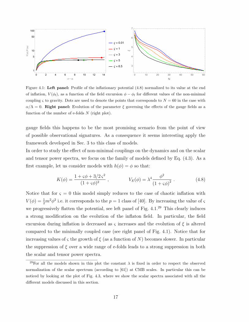
Figure 4.1: Left panel: Profile of the inflationary potential (4.8) normalized to its value at the end
of inflation, V (φf), as a function of the field excursion φ − φf for different values of the non-minimal
coupling ς to gravity. Dots are used to denote the points that corresponds to N = 60 in the case with
α/Λ = 0. Right panel: Evolution of the parameter ξ governing the effects of the gauge fields as a
function of the number of e-folds N (right plot).
gauge fields this happens to be the most promising scenario from the point of view
of possible observational signatures. As a consequence it seems interesting apply the
framework developed in Sec. 3 to this class of models.
In order to study the effect of non-minimal couplings on the dynamics and on the scalar
and tensor power spectra, we focus on the family of models defined by Eq. (4.3). As a
first example, let us consider models with h(φ) = φ so that:
K(φ) =1 + ςφ+ 3/2 ς2
(1 + ςφ)2, VE(φ) = λ4 φ2
(1 + ςφ)2 . (4.8)
Notice that for ς = 0 this model simply reduces to the case of chaotic inflation with
V (φ) = 12m2φ2 i.e. it corresponds to the p = 1 class of [40]. By increasing the value of ς
we progressively flatten the potential, see left panel of Fig. 4.1.29 This clearly induces
a strong modification on the evolution of the inflaton field. In particular, the field
excursion during inflation is decreased as ς increases and the evolution of ξ is altered
compared to the minimally coupled case (see right panel of Fig. 4.1). Notice that for
increasing values of ς the growth of ξ (as a function of N) becomes slower. In particular
the suppression of ξ over a wide range of e-folds leads to a strong suppression in both
the scalar and tensor power spectra.
29For all the models shown in this plot the constant λ is fixed in order to respect the observed
normalization of the scalar spectrum (according to [61]) at CMB scales. In particular this can be
noticed by looking at the plot of Fig. 4.3, where we show the scalar spectra associated with all the
different models discussed in this section.
17

10-15 10-10 10-5 100 105
10-15
10-11
10-7
0102030405060
f[Hz]
ΩGWh2
N
ς = 0.01, = 1
ς = 0.01, = 10
ς = 1, = 1
ς = 1, = 10
ς = 3, = 1
ς = 3, = 10
ς = 5, = 1
ς = 6.5, = 1
Figure 4.2: Power spectrum of tensor perturbations for all the models of Fig. 4.1 (dashed lines corre-
sponds to models with N = 10). We are also showing the sensitivity curves for (from left to right):
milli-second pulsar timing, LISA, advanced LIGO. Current bounds are denoted by solid lines, expected
sensitivities of upcoming experiments by dashed lines. See main text for details on these curves.
As described in Sec. 3, the changes in the tensor spectrum are simply due to the
different evolution of ξ. In particular, as for increasing values of ς the growth of ξ
becomes slower over a broad range of N -values, we expect the GW spectrum (which is
exponentially sensitive to ξ) to be strongly suppressed. This effect is clearly visible in
Fig. 4.2 where we compare the GW spectra for the models of Fig 4.1 with the sensitivity
curves of some current (solid lines) and upcoming (dashed lines) direct GW detectors.
For the millisecond pulsar timing arrays covering frequencies around 10−10 Hz, we
show the constraint depicted in Ref. [80], the update from EPTA [81] and the expected
sensitivity of SKA [82]. The laser interferometer space antenna (LISA) [2] is a future
mission designed to probe the mHz range [39,83,84], where as ground-based detectors
are sensitive at a few 10 Hz (LIGO/VIRGO [85]). It is interesting to notice that for
ς ∼ 1 the spectrum is marginally detectable (for N = 10) by LISA but not by advanced
LIGO. For larger values of ς the suppression of the spectrum is so strong that the signal
is well below the expected sensitivities of upcoming GW detectors.
In Fig. 4.3 we show the scalar power spectrum (corresponding to Eq. (3.29)) for all
the models shown in the previous plots. Notice that, in order to respect the COBE
normalization (that sets the amplitude of the spectrum at CMB scales) all the spectra
meet at the same value for N ' 60. Moreover, it is worth mentioning that all the
18

0 10 20 30 40 50 6010-9
10-8
10-7
10-6
10-5
10-4
10-3
N
Δs2
ς = 0.01, = 1
ς = 0.01, = 10
ς = 1, = 1
ς = 1, = 10
ς = 3, = 1
ς = 3, = 10
ς = 5, = 1
ς = 6.5, = 1
Figure 4.3: Scalar power spectrum for all the models of Fig. 4.1 (dashed lines corresponds to models
with N = 10). The lower horizontal line denotes the observed normalization at CMB scales (according
to [61]) and the upper horizontal line is the estimate of [33] for the PBH bound. More details on this
bound on the generation of PBHs are reported in Sec. 5.
models shown in this section are in agreement30 with the constraints set by Planck
on ns and r and on the generation of primordial non-Gaussianities.31 Interestingly,
for none of the models shown in this plot the spectrum features a peak. This can be
explained by considering the expression of K(φ) in terms of N . While for ς 1 K(φ)
is essentially constant, for sizable values of ς we have K(φ) ∝ 1/(ςN)2 to leading order
in N . By numerically solving the evolution it is possible to show that K(φ) becomes
large only for N ' 2÷4 depending on the model, and the suppression of ξ is not strong
enough to disrupt its monotonic growth before the end of inflation. As a consequence,
in order for the spectrum to feature a peak, we require a strong growth of K(φ) at
sufficiently large values of N . Such a behavior can be achieved by considering different
parameterizations for h(φ).
As discussed in Ref. [40], the scalar and tensor spectra in axion inflation can be well
understood in terms of universality classes of inflation [76–78], categorized by the scaling
of εH(N) in the regime where the back-reaction of the gauge fields is weak. This is
immediately understood (for a minimal coupling to gravity) since the growth of both
the scalar and tensor spectrum is driven by ξ ∝ √εH . However, when a non-minimal
30Except for the model with ς = 0.01, for which the predicted value of r is marginally excluded by
Planck [61] at 95% CL.31 This can directly be checked from Fig. 4.1, ξ|CMB . 2.5.
19

coupling is considered, the instability is controlled by ξ ∝√εH/K (see Eq. (3.22)).
Whereas the examples depicted so far correspond to εH/K ∝ 1/Np with p . 1 [78],32
different behaviors can be achieved. In particular here, in order to obtain a scalar
spectrum which rises at larger values of N (i.e. at an earlier stage during inflation) we
require a quicker increase of εH(N), with decreasing N . At the same time, in order to
obtain a suppression of ξ which leads to the appearance of a bump in the spectra, we
also require the kinetic function K(N) to become sizable at sufficiently large values of
N . A simple example of this type can obtained by choosing:
h(φ) = (1− 1/φ) , VE(φ) = λ4 (φ− 1)2
(φ+ ς(φ− 1))2 , (4.9)
which for a vanishing non-minimal coupling and a vanishing coupling to gauge fields
(ς = 0, α = 0) leads to εH ∝ 1/N4/3 while the kinetic function K(N) interpolates from
an approximately constant behaviorw at large N to K(N) ∝ e−N at small N . We will
also return to models of this type when discussing PBH dark matter.
In Fig. 4.4 we depict the evolution of the parameter ξ for some representative models
of the class defined by Eq. (4.9). As before, the normalization of the scalar potential is
fixed by the COBE normalization that fixes the amplitude of the scalar power spectrum
at CMB scales and we ensure agreement with all CMB constraints. The remaining
parameters are chosen to obtain sizable gauge-field induced effects while conveying
an idea of the possible parameter space. We clearly see the peaked features around
N ' 20−40 in all spectra with a significant value of the non-minimal coupling ς, which
translates into a broad peak in the scalar and tensor spectra, depicted in Fig. 4.5. For
increasing values of α/Λ and ς the bump in the spectra shifts to larger values of N
i.e. to larger scales. This is consistent with the physical intuition: For larger values of
α/Λ the increase in the spectrum arises earlier (see also [40]), for larger values of ς the
subsequent suppression due to the non-canonically normalized kinetic term takes effect
at earlier times. Moreover, increasing ς we reduce the field excursion during inflation,
leading to a suppression of ξ over a broad range of N -values. As a consequence (and
32While it is easy to see that p = 1 for ς = 0 (see [78]), this statement may seem surprising for
ς 6= 1, when the scalar potential asymptotically approaches the exponentially flat Starobinsky-like
potential (that for a minimal coupling is characterized by εH ∝ 1/N2 [78]). This subtlety arises due
to the coupling of the gauge fields to the canonically normalized inflaton field of the Jordan frame.
By considering the expression of K(φ) given in Eq. (4.3) and using the definition N ≡∫ √
K/2εH dφ,
one finds that ξ ∝√εH/K is in fact independent of N at small values of N (ignoring here a possible
black-reaction of the gauge-fields).
20

0 10 20 30 40 50 60
1
2
3
4
5
6
10-1510-1010-5100105
N
ξ
f[Hz]
ς = 0.01, = 1
ς = 55, = 1
ς = 45.7, = 1
ς = 65.5, = 1
Figure 4.4: Evolution of ξ as a function of N for models based on Eq. (4.9). The model parameters
are chosen to obey CMB and PBH constraints, see main text for details. In particular, the depicted
curves are obtained for couplings to the gauge-fields of α/Λ ' 97, 63, 71, 74 (for increasing value of
the non-minimal coupling to gravity ς, respectively).
indeed consistently with Fig. 4.2 and Fig. 4.3), increasing the non-minimal coupling ς
we note a suppression both in the scalar and tensor power spectra. For ς ' 63 and 71
the signal is below the predicted sensitivity of LISA by roughly an order of magnitude.
Finally, we point out that the peaks in the scalar spectrum of Fig. 4.5 correspond to
values of ξ . 4.6. Contrary to the case of minimal coupling, we do hence not enter
into the regime ξ & 4.8 where perturbativity breaks down [86] and where significant
uncertainties become attached to the predictions for the scalar spectrum.
Let us conclude this section by summarizing the key feature of K(φ) and V (φ) which
allow for the appearance of a peak in the spectra within the last 60 e-folds. A first
requirement is that the instability occurs at sufficiently large values of N . This can be
rephrased as the requirement that ξ ∝√εH/K grows sufficiently fast with decreasing
N for large values of N . After this first regime, we need the effects of the non-canonical
kinetic term to become important. Concretely, in order to observe a bump in the spectra
we require a rapid increase in K(φ) at a sufficiently large value of N (for example at
N ' 20). As the growth of K(φ) turns into a suppression of ξ, this mechanism shuts
off the instability, leading to the appearance of a bump both in the scalar and tensor
power spectra. To illustrate this we chose to study two example models as defined by
21
10-15 10-10 10-5 100 105
10-15
10-11
10-7
0102030405060
f[Hz]
ΩGWh2
N
ς = 0.01, = 1
ς = 55, = 1
ς = 45.7, = 1
ς = 65.5, = 1
0 10 20 30 40 50 60
10-11
10-8
10-5
10-2
N
Δs2
ς = 0.01, = 1
ς = 55, = 1
ς = 45.7, = 1
ς = 65.5, = 1
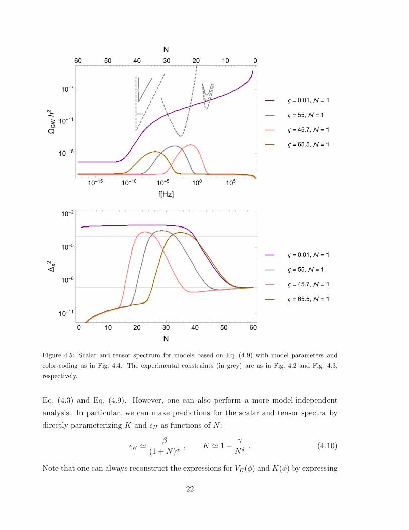
Figure 4.5: Scalar and tensor spectrum for models based on Eq. (4.9) with model parameters and
color-coding as in Fig. 4.4. The experimental constraints (in grey) are as in Fig. 4.2 and Fig. 4.3,
respectively.
Eq. (4.3) and Eq. (4.9). However, one can also perform a more model-independent
analysis. In particular, we can make predictions for the scalar and tensor spectra by
directly parameterizing K and εH as functions of N :
εH 'β
(1 +N)α, K ' 1 +
γ
N δ. (4.10)
Note that one can always reconstruct the expressions for VE(φ) and K(φ) by expressing
22
N as a function of φ. Hence, in case of a detection of peaks in the scalar and tensor
spectra one could determine the corresponding expressions for VE(φ) and K(φ).
5 Primordial black holes
5.1 A quick review of PBH formation
The models discussed in the previous sections generically lead to a strong enhancement
of the scalar power spectrum at small scales. If the scalar fluctuations are sufficiently
large, this leads to the formation of PBHs in the subsequent evolution of the universe.
Here we briefly review the resulting PBH distribution following Ref. [13], collecting the
relevant tools to apply this formalism to our discussion.
Primordial scalar fluctuations with a power spectrum P (ζ) form PBHs upon re-entry
into the horizon if ζ > ζc. The mass M of the resulting black hole can be estimated to
be determined by the mass MH contained in the horizon at the time of horizon re-entry
tN ,
M(N) = γMH ' γ4πm2
p
Hinf
ejN ' 55 g γ
(10−6mp
Hinf
)ejN , (5.1)
with N counting the number of e-folds from the end of inflation when the fluctuations
in question exited the horizon, Hinf denoting the Hubble parameter at this time and j
parameterizing if the equation of state between the end of inflation and the re-entry of
the fluctuation was mainly matter dominated (j = 3) or radiation dominated (j = 2).
In the setup of Sec. 2 we expect reheating to be efficient due to the inflaton gauge field
coupling. In the following we will thus work with j = 2. Finally, γ is a numerical
factor depending on the details of the gravitational collapse. Following [6, 87] we will
use γ = 0.4.
The fraction of the energy density of the universe which collapses into PBHs at any
given time tN is given by
β(N) =
∫ ∞ζc
M(N)
MH(N)PN(ζ) dζ =
∫ ∞ζc
γ PN(ζ) dζ . (5.2)
Here PN(ζ) denotes the probability distribution of fluctuations sourced at N e-folds
before the end of inflation. In our case, the fluctuations are characterized by a strong
equilateral non-Gaussianity [38], and can in particular be expressed as ζ = g2 − 〈g2〉with g ∝ ( ~E · ~B)1/2 following a Gaussian distribution (see Eq. B.3) [33]. For such a
23

positive χ-squared form of non-Gaussianities, the probability distribution is given by
(see e.g. [88–90]):
PN(ζ) =exp
(− ζ+σ2
N
2σ2N
)√
2πσ2N(ζ + σ2
N), (5.3)
with σ2N = (∆2
s(N))1/2 and∫∞−σ2
NPN(ζ) dζ = 1. Since Eq. (5.1) provides a unique rela-
tion between the time of formation tN and the mass of the PBH M , we can equivalently
express the fraction β(N) dN of the universe collapsing in the time interval [tN , tN+dN [
as a function of the PBH mass M :
β(N) dN = β(M)dN
dMdM =
β(M)
2MdM . (5.4)
We stress that β denotes the fraction of the universe collapsing into PBHs at the
respective time of formation. Within the ΛCDM model, we can translate this to the
fraction of the energy density in the Universe at some later time. Ignoring the decay of
PBHs for the moment (we will return to this point below) and assuming an adiabatically
expanding universe, the ratio of the number density of PBHs nPBH(t) and the entropy
s(t) is constant. We can hence relate the function β(M) to the number density of PBHs
at any later time t as [13]:
β(M) =MnPBH(tN)
ρ(tN)=
4M nPBH(t)
3T (tN) s(t), (5.5)
with ρ(tN) = 3/4T (tN) s(tN) denoting the energy density of the Universe, assuming
that the universe is dominated by radiation at tN . The temperature T (tN) is related to
H(tN) = Hinf exp(−2N) through the Friedmann equation. Substituting Hinf exp(−2N)
into Eq. (5.1), we find that the fraction of dark matter today formed by PBHs is
f(M) =MnPBH(t0)
ΩCDM ρc'
' 4.1 · 108 γ1/2
(g∗(tN)
106.75
)−1/4(h
0.68
)−2(M
M
)−1/2
β(M) , (5.6)
where we have inserted ρc = 3H20m
2p with H0 = h 100 (km/s)/Mpc for the critical
density and ΩCDM ' 0.21 for the dark matter fraction today. In the following, we will
set h = 0.68 and g∗(tN) = 106.75. PBHs with masses below MPBH < M∗ ' 5 · 1014 g
have a life time shorter than the current age of the universe and would have evaporated
through Hawking radiation by now.33 The interpretation of f(M) as the fraction of
33The numerical value M∗ might be enhanced when taking into account accretion and merger pro-
cesses in the matter dominated regime which stabilize light PBHs, see App. C.
24

dark matter hence only applies for M > M∗, for smaller values of M the ratio f(M)
may simply be seen as a convenient way of parameterizing the initial PBH abundance
β(M).
The production of PBHs is subject to various constraints, see Ref. [13] for an overview
and Ref. [6] for updated bounds on the mass range M > M∗, which will be the range
most relevant for us here. As pointed out in Ref. [6], applying these bounds to an
extended mass function requires some care. Essentially, a flat constraint fmax in a
certain mass range implies that the total amount of PBHs in this mass range may
not exceed the value fmax. A general constraint can then be treated as a sequence of
approximately flat constraints. Here we follow the procedure suggested there, requiring∫ M2
M1
dM
2Mf(M) < f [M1,M2]
max , (5.7)
with the constraints fmax taken from Tab. 1 of Ref. [6] and f[M1,M2]max denoting the weakest
constraint in the mass range [M1,M2]. Here we vary the integration boundaries M1,2
so that all relevant mass intervals are covered. We have used Eq. (5.4) to obtain a
dimensionless integrand in Eq. (5.7).
We note that the PBH formation as sketched above is subject to theoretical uncertain-
ties, in particular concerning the effects of critical collapse, non-spherical properties
of the primordial fluctuations and late time accretion and mergers. We discuss these
issues in more detail in App. C. The upshot is that these uncertainties are to large
degree degenerate with our model parameters, and hence will not change the overall
picture presented here.
5.2 PBHs in models with non-minimal coupling to gravity
In Fig. 5.1 we depict two typical results for f(M) for the first model discussed in
Sec. 4, characterized by a non-minimal coupling to gravity through h(φ) = φ. The
parameters34 α/Λ, m, ς and N are chosen to meet the following conditions: (i) the
amplitude and spectral tilt of the scalar spectrum at the CMB scales match the observed
values, (ii) the effect of the gauge field contribution is maximized while respecting
the CMB non-Gaussianity bounds and (iii) the PBH abundance is maximized while
respecting the depicted PBH bounds. Moreover, the orange curve corresponds to the
situation which roughly maximizes the contribution to PBH dark matter in this setup.
34Here m2 = 2λ4 in Eq. (4.3).
25

ς = 3, = 9
ς = 5, = 5
M*
10 105 109 1013 101710-29
10-19
10-9
10
0 5 10 15 20
M [g]
f(M)
N
Figure 5.1: Would-be fraction of PBH dark matter, compared to the constraints in Ref. [6, 13] for
models based on Eq. (4.8). The parameters of these curves are chosen to maximize the PBH contribu-
tion while obeying the depicted PBH bounds as well as the CMB constraints. Note that the quantity
f(M) corresponds to the fraction of dark matter today only for M > M∗ ' 5 · 1014 g.
The parameter values for the depicted curves are m = 7.6 · 10−5mp, α/Λ = 43.2 for
the ς = 5 example and m = 5.4 · 10−5mp, α/Λ = 37 for the ς = 3 example. The
resulting mass functions increase towards low PBH masses at M M∗, hence only the
high-mass tails of these distributions can contribute to PBH dark matter today. The
strongest constraints close to the dark matter threshold come from evaporating PBH
around M ∼M∗, which leave traces in the anisotropies of the CMB and in the (extra-)
galactic photon background (see [13] for details), which imply β(M) . 10−28 in this
mass range. For the depicted examples, we find for the scalar spectral index ns, the
tensor-to scalar ratio r and the fraction of PBH dark matter ftot,
ς = 5 : ns = 0.98 , r = 1 · 10−3 , ftot ≈ 0 , (5.8)
ς = 3 : ns = 0.97 , r = 5 · 10−3 , ftot = 3 · 10−23 . (5.9)
To obtain a mass distribution peaked at heavier PBHs, we need to modify the func-
tional dependence of the non-minimal coupling, h(φ). In particular we require a scalar
spectrum which rises at larger values of N , i.e. at an earlier stage during inflation. As
discussed in Sec. 4, this can be realized by considering for example h(φ) = 1− 1/φ. In
this case, for sufficiently large values of ς the scalar spectrum features a peak at large
scales (see Fig. 4.5) that can suitably induce the generation of a distribution of PBHs.
The exact position and the shape of the peak are controlled by the parameters α/Λ
26

1016 1021 1026 1031 103610-10
10-8
10-6
10-4
0.01
1
100
20 25 30 35 40 45
M [g]
f(M)
N
ς << 1, = 1
ς = 55, = 1
ς = 45.7, = 1
ς = 65.5, = 1
Figure 5.2: Fraction of energy in PBH at time of formation, compared to the constraints in Ref. [6],
for models based on Eq. (4.9). Model parameters and color coding as in Fig. 4.4. Compatibility with
the depicted constraints is confirmed using Eq. (5.7).
and ς. In particular, increasing the value of ς moves the peak towards larger values
of N (see also Fig. 4.5) and suppresses the amplitude, whereas increasing the value
of α/Λ enhances the spectrum while also shifting the peak towards larger values of N
(see e.g. [40]). Since both parameters also impact the CMB observables, the depicted
curves roughly demonstrate the range of possibilities for this choice of h(φ).
For the examples shown in the plot of Fig. 5.2 we have:
ς = 45.7, α/Λ ' 63 : ns = 0.963 , r = 3.2 · 10−4 , (5.10)
ς = 55, α/Λ ' 71 : ns = 0.957 , r = 3.3 · 10−4 , (5.11)
ς = 65.5, α/Λ ' 74 : ns = 0.958 , r = 7.4 · 10−4 . (5.12)
For reference, we also show the result for a negligible non-minimal coupling (purple
curve). The bumps in the spectra for the three models shown in Fig. 5.2 lead to the
generation of PBH distributions peaked around M ∼ 1020, 1025 and 1031 g, respectively,
thus in all three cases the entire PBH population contributes to dark matter today. In
all cases we restrict ourselves to a single gauge field, N = 1. As in Fig. 5.1, the model
parameters for these benchmark points have been chosen in order to maximize the PBH
contribution while obeying all relevant bounds. The reduced amplitude for the ς = 65.5
example is due CMB constraints which become more relevant as α/Λ is increased.
In this mass range, the strongest constraints come from neutron star capture [91] as
27

well as from micro lensing constraints from the Kepler, MACHO, EROS and OGLE
experiments [92–94]. In particular, the micro lensing constraints restrict the total
amount of PBHs to be less than 4% to 30% in their respective mass ranges, whereas
the neutron star capture constraint requires the total amount of PBHs to be less than
6% for 1018 g . M . 1024 g. This last constraint (shown as a dashed curve in
Fig. 5.2) has been disputed, as it relies on assumptions about the dark matter content
in globular clusters [6]. For the pink curve in Fig. 5.2 we thus choose to omit this
constraint, demonstrating that in this case PBHs can account for all of dark matter.35
Of course, if new results confirm this bound, the fraction of PBH dark matter in this
mass range must be less than the 6% mentioned above.
The total fraction of PBH dark matter today is given by
ftot =ΩPBH
ΩCDM
=
∫ ∞M∗
dM
2Mf(M) , (5.13)
where in practice we need to integrate only over the strongly enhanced part of the
scalar spectrum, as it is well-known that the contribution from the spectrum at CMB
scales (where the amplitude is fixed by CMB observations) is completely negligible.36
For example, for the curves in Fig. 5.2 we find
f ς=45.7tot = 98.6%, f ς=55
tot = 39.4%, f ς=65.5tot = 1.2 · 10−4 % . (5.14)
In summary, while for the h(φ) = φ case the contribution to dark matter is completely
negligible, PBHs can contribute a very significant fraction of dark matter for h(φ) =
1− 1/φ in this setup.
5.3 Searching for PBHs with GW interferometers
PBHs can form binary objects which source GWs similar to the event observed by
LIGO [1]. In this subsection, we address the question if these GWs may be observable in
future GW interferometers, see also [9]. We will normalize the results of this subsection
35Upon finalizing this paper, we became aware of the very recent microlensing constraint from the
Subaru Hyper Suprime-Cam [95], which sets strong constraints on most of this window, leaving only a
narrow slice around M ' 1020 g for a significant PBH contribution to dark matter in this mass range.36Strictly speaking, our analysis here applies only to PBH formed in the radiation dominated regime,
i.e. for M < M(Neq) with Neq ' NCMB− 1.2 labeling the primordial fluctuations entering the horizon
at matter-radiation equality. However as these scales are strongly constrained by the CMB, we do not
need to worry about this subtlety.
28

to M = M = 1.99 · 1033 g, which roughly corresponds to the brown curve in Fig. 5.2
after taking into account the mass increase of the PBH during the matter dominated
phase due to accretion and mergers (see App. C).
Let us first consider GW signal from inspiraling PBHs (see e.g. [67]). Comparing the
orbital distance of two (point-like) objects rotating with frequency ω,
Rorb =(GMsys/ω
2)1/3
, (5.15)
where G = 6.67 · 10−11m3/(kg s2) and Msys is the sum of the two masses, to the sum of
the Schwarzschild radii,
Rschw = GMsys/c2 , (5.16)
we find for the peak frequency of the GW signal of a black hole binary, f = ω/π,
fmax ∼ 6.4 · 104 Hz
(2 ·MMsys
). (5.17)
For comparison, the frequency band of LIGO extends to about few times 103 Hz. In the
early inspiral phase, the system will emit GWs at lower frequencies, thus potentially
‘crossing’ the LIGO frequency band as the system approaches coalescence. The time τ
between when signal is at the LIGO peak sensitivity of f ∼ 100 Hz and coalescence is
given by
τ = 3 s
(MMc
)5/3(100 Hz
f
)8/3
, (5.18)
where Mc is the so-called chirp mass, M5c = (M1M2)3/(M1 + M2), constructed from
the masses of the two individual BHs. The amplitude of the emitted GWs, detected at
a distance r from the source is given by
h ' 4
r
(GMc
c2
)5/3(πf
c
)2/3
. (5.19)
Comparing this to the strain sensitivity of advanced LIGO, h ' 10−24/√
Hz [96], we
find that assuming a bandwidth of 10 Hz, a signal originating from a binary BH system
can be detected if a source is within
r = 8.0 · 102 Mpc
(Mc
M
)5/3(f
100 Hz
)2/3
(5.20)
of the detector. For comparison, the size of the Milky Way is about 30 - 55 kpc and
the size of the Virgo super cluster is about 33 Mpc. This has to be compared to the
expected rate of BH mergers, which has been estimated to be [3–5]
Γ = 10−8 ftot δlocPBH yr−1 Gpc−3 . (5.21)
29
Here δlocPBH denotes the local PBH density contrast, where δloc
PBH = 1 yields the expected
merger rate if PBH are distributed uniformly throughout the universe. Clustering of
PBHs into sub-halos may however increase the value to δlocPBH ∼ 107 − 109 [4], dramati-
cally enhancing the prospects for detection. Note that Eq. (5.21) is independent of the
PBH mass, which drops out when combining the dark matter number density and the
BH - BH capture cross section (see e.g. [3]). Hence for M ∼ M and ftot = O(0.1)
one might indeed expect a handful of these events per year at f = 102 Hz, baring in
mind the huge uncertainty in δlocPBH. Note however that since the reach of the detector is
sensitive to the PBH mass (see Eq. (5.20)), the total rate drops significantly for lighter
PBHs.
In addition to the transcendent GWs signal from PBH binaries discussed above, there
will also be a diffuse stochastic background arising from binaries which are too faint
to be detected as individual sources. For a recent analysis see Ref. [7], where it was
concluded that depending on the PBH merger rate (see above) and the shape of the
PBH distribution, such a stochastic background might indeed be detectable by LISA.37
5.4 Discussion
The peaks of the mass distributions in Fig. 5.2 are in an interesting mass region. In the
lower mass region (pink and grey curves) the bounds on f(M) are weaker (in particular
if one omits the neutron star capture bound), and it becomes possible to account for
a significant fraction, or maybe even all of dark matter, in PBHs. Moreover, the mass
ranges found in these benchmark models lie below the lower bound expected from
BHs formed in stellar evolution, M & 3M [97]. If detected, such light BHs thus
immediately point towards a possible primordial origin. On the other hand, the higher
mass region (brown curve) provides PBHs which might be in the correct ballpark to
be detected through their gravitational wave signatures in advanced LIGO. However,
we emphasize that for the specific, simple choice of h(φ) discussed here, the abundance
of PBHs in this mass range is strongly constrained by CMB observations, rendering a
detection with LIGO very challenging even for large density contrasts δlocPBH.
We stress that the spectra depicted in Fig. 5.2 are not a unique prediction but only
three representative benchmark models. Clearly, varying the parameters (as discussed
37In addition, the formation process of BPHs may lead to a stochastic GW background similar to
first order phase transitions [9].
30
in Sec. 4) the amplitude of this signal can be adjusted. Moreover, as can be seen by
comparing Figs. 5.1 and 5.2, the position of the peak is very sensitive to the choice of
the function h(φ). In this context, we point out that Ref. [6] recently identified two
interesting ‘windows’ for PBH dark matter, in which dark matter could still consist of
PBH to 100%. The lunar BH window MPBH ∼ 1020 − 1024 g opens when omitting the
neutron star capture constraint, as mentioned above. The second window is located at
MPBH ∼ 1M − 103M (LIGO-like BHs) and may be reached by either considering
more complicated functions h(φ) or by a better understanding of the accretion and
merger processes in the matter dominated regime.
Given the different spectra depicted in Fig. 4.3, one might wonder if a sizable PBH
population might be achieved without invoking a non-minimal coupling to gravity, i.e.
for ς = 0. In this case the characteristic feature of the scalar spectrum is a plateau
extending to small scales. The function β(M) will hence also be constant, and the
strongest constraint come from searches for anisotropies in the CMB and for anomalies
in the (extra-) galactic photon background, restricting β . 10−28 at M ∼ 1013 g [13].
This implies f ∼ 10−20 (M/M)1/2. Integrating over the entire range which could
contribute to PBHs, the lower bound M > 5 · 1014 g dominates the integral leading to
ftot . 10−11, i.e. a completely negligible fraction of dark matter. In the setup discussed
here, the non-minimal coupling ς is hence essential to obtain a significant fraction of
dark matter in PBHs.
6 Conclusion and Outlook
Axion-like particles are one of the most natural candidates to drive cosmic inflation
since their perturbative shift-symmetry protects the flatness of their potential against
quantum corrections. These pseudoscalar fields typically couple to the gauge fields
present in the theory through a Chern-Simons term in the Lagrangian. As reviewed in
Sec. 2, in models of axion-inflation, such a coupling can lead to several interesting and
possibly observable phenomenological features. In particular, the production of chi-
ral gravitational waves is a peculiar signature of these models that could be observed
in the near future in experiments like the ground-based interferometer LIGO or the
space-mission LISA. Hence, it is extremely interesting to continue exploring the rich
phenomenology provided by these inflationary models. In this paper we showed that if
the axion-inflaton is non-minimally coupled to gravity, these models of axion-inflation
31

represent a natural framework for the production of PBH dark matter. In particular,
in Sec. 3 we worked out the main generic features of an axion-inflation model with
non-minimal coupling to gravity, deriving both the background dynamics and the per-
turbation power spectra. As explained in Sec. 4, the interplay between the two main
features of this model, i.e. the coupling to gauge fields and the non-minimal coupling
to gravity, makes the generation of a broad peak in the scalar spectrum possible. In
particular, the increase of the spectrum is sourced by the instability caused by the
coupling between the inflaton and the gauge fields. If the kinetic function K(φ) (see
Eq. 3.4), corresponding to a non-minimal coupling to gravity in the Jordan frame,
features a rapid increase after the advent of this instability, a subsequent suppression
of the spectrum arises, generating a peak as shown in Fig. 5.2. The position of the
peak is determined by the choice of K(φ) and by the ratio α/Λ (see Eq. 3.4), which
parametrizes the strength of the inflaton coupling to gauge fields. In this context,
an interesting class of models is given by the attractors at strong coupling, defined in
Eq. (4.3). As shown in Sec. 5, by choosing the kinetic function K(φ) in such a way
that the previously mentioned condition is met (see Eq. (4.9)), PBHs produced with
this mechanism can account for a sizeable fraction of the dark matter present in the
universe in a wide region of the parameter space. As explained in the main text, if we
ignore the disputable bounds based on neutron star capture, PBHs can even account
for the totality of dark matter, in the mass range 1018 g − 1024 g. Heavier PBHs with
masses around a solar mass, although accounting only for a fraction of dark matter,
may in turn lead to observable GW signals in LIGO.
The inflationary model employed and the PBH production mechanism proposed in
this paper can be further developed following several complementary directions. For
instance, they should be embedded in a consistent cosmological scenario, which includes
the reheating of the Standard Model degrees of freedom. Since the inflaton is coupled
to gauge fields, (p)reheating would primarily produce these massless vector fields [98].
If the number of gauge fields N is larger than one38, this could lead to a tension with
the constraints on the amount of dark radiation present in the universe at the time of
Big Bang Nucleosynthesis and of recombination [75] if the gauge fields remain massless.
Hence, the inclusion of the Standard Model degrees of freedom and of the (p)reheating
should be consistent with these bounds. A detailed study of the (p)reheating process
could also provide interesting clues for the generation of the baryon asymmetry of the
38Or if N = 1 but the related gauge field is not the Standard Model hypercharge.
32
universe, possibly sourced by the CP-violating axion-gauge field coupling [99–101].
The high sensitivity of inflation to quantum corrections makes it crucial to embed any
effective model into an UV complete theory. As remarked in App. A, string theory
contains all the ingredients necessary for the realization of an explicit embedding of the
PBH production mechanism described in this paper: inflaton-dependent non-canonical
kinetic terms for the axion-inflaton, a potential that supports axion-inflation and a
coupling between the axion-inflaton and topological terms of Abelian gauge theories.
The realization of an explicit string theory construction is beyond the scope of this
paper, and we leave it for future work.
In Sec. 5 we have only reported a few benchmark models in order to show that the
mechanism is well-suited for the production of PBHs. It would be interesting to perform
a systematic analysis in order to understand which choices of the scalar potential and
of the non-minimal coupling to gravity lead to the production of PBHs that compose
a sizable fraction of the dark matter present in the universe - or vice versa how to
reconstruct these fundamental ingredients of the theory for a given PBH distribution.
Finally, it would be interesting to extend this inflationary model to the case in which
the axion-inflaton is coupled to non-Abelian gauge fields, and to study how the PBH
production would be modified in such a setup.
Acknowledgements
We thank D. Figueroa, E. Kiritsis, A. Kusenko, and L. Sorbo for valuable comments
and discussions at various stages of this work. We are especially indebted to Pierre
Binetruy who, to our great sorrow, unexpectedly passed away during the completion
of this work. Pierre sparked our interest in this topic, and his advice and guidance was
invaluable in the early stages of this work.
We acknowledge the financial support of the UnivEarthS Labex program at Sorbonne
Paris Cite (ANR-10-LABX-0023 and ANR-11-IDEX-0005-02) and the Paris Centre for
Cosmological Physics. L. W. is partially supported by the Advanced ERC grant SM-
grav, No 669288. V. D. would like to thank the Berkeley Center for Theoretical Physics
for kind hospitality during the final stages of this work. F. M. is supported by the
European Research Council starting grant ‘Supersymmetry Breaking in String Theory’
(307605).
33

A Axions in field theory, supergravity and string
theory
A brief review of the QCD axion
An axion-like particle (axion, for short) is a pseudoscalar particle φ that enjoys a
continuous perturbative shift-symmetry of the form
φ→ φ+ a , (A.1)
where a is a real constant. Historically, axions arose in field theory to solve the long-
standing strong-CP problem of QCD [102]. The symmetries of QCD allow for a topo-
logical term in the Lagrangian
LQCD ⊃θ
32π2trFµνF
µν , (A.2)
where Fµν is the QCD field strength. Such a term violates the CP symmetry and would
give rise to an electric dipole moment for the neutron in contrast with observations,
unless the parameter θ is tuned very small . 10−10 [103].39 The introduction of an axion
φ, proposed by Peccei and Quinn [104–106], solves this naturalness problem of QCD.
The field φ couples with the topological term (φ/f) FF , giving rise to an effective θ
parameter
θeff = θphys +φ
f, (A.3)
where f is the axion decay constant. Due to the shift-symmetry of the theory, θphys can
be absorbed into the axion field. The shift-symmetry is broken by non-perturbative
effects [107] (instantons in the case of QCD) to a discrete shift symmetry of the form
φ→ φ+ 2πf , (A.4)
and a cosine-like potential for the axion is generated
V (φ) = muΛ3QCD
[1− cos
(φ
f
)], (A.5)
where ΛQCD is the QCD scale and mu is the mass of the up quark. Such a potential
dynamically sets the coefficient of the topological term to zero. This procedure is very
39The physical quantity is θphys = θ + arg (det (MuMd)), where Mu and Md are the quark mass
matrices. The shift comes from a chiral rotation of quark fields in the Standard Model Lagrangian.
34

generic: non-perturbative effects always induce cosine-like potentials for axions. A
coupling φFF between the axion and the topological term is also allowed for Abelian
gauge groups, i.e. such a term is generically not forbidden by any symmetries. This
is the basis for the coupling between the axion and Maxwell theory considered in this
paper.
An axionic field with a coupling of the form φFF is often associated with theories
exhibiting global chiral or gauge anomalies. In the case of a gauge anomaly the axion
is eaten by the gauge boson, giving rise to a consistent effective theory with a massive
gauge boson. As a result the axion is removed from the low energy spectrum. This
can be avoided in more complicated constructions with multiple U(1) factors and a
carefully chosen fermion spectrum [108]: In particular, one can construct theories with
massless gauge bosons that couple to axions as φFF .
Axions as inflaton fields
Due to their perturbative shift-symmetry, axions are one of the most natural candidates
to drive inflation: such a symmetry protects the flatness of their scalar potential against
quantum corrections. The arguably simplest axion inflation model employs the cosine
potential (A.5).40 Note that inflation models based on such an oscillatory potential are
models of large-field inflation: the slow-roll conditions are satisfied for φ & mp. As the
potential is periodic, this implies that the period needs to take super-Planckian values,
i.e. natural inflation requires f & mp.
More general inflationary potentials can only be generated if the shift-symmetry is
broken completely. If the breaking is explicit, the protection from quantum corrections
would generically be lost. However, we can retain a sufficient level of control by only
breaking the shift-symmetry weakly: note that it is technically natural to take the
symmetry-breaking terms to be small. Then the quantum corrections resulting from
the breaking are also suppressed. Another way of preserving the protection offered by
the shift-symmetry is to only break it spontaneously. This can be realized by coupling
the axion to a 3-form theory [109–111]. To be explicit, consider the theory of an axion
φ and a 3-form Cνρσ with corresponding field strength Fµνρσ = 4∂[µCνρσ] described by
40The inflationary potential is obtained from eq. (A.5) substituting muΛ3QCD → Λ4, where Λ is the
scale of non-perturbative effects that generate the potential for the inflaton, i.e. V = Λ4 [1− cos (φ/f)].
35

the following Lagrangian density:
L =1
2(∂φ)2 − 1
48F 2µνρσ +
µ
24φ εµνρσFµνρσ . (A.6)
Here µ is a parameter with the dimensions of mass. As a 3-form does not have any
propagating degrees of freedom in 4 dimensions, it can be integrated out, leading to
L =1
2(∂φ)2 − 1
2(q + µφ)2 , (A.7)
where the parameter q corresponds to a VEV for F4 [110]. Thus one arrives at a
non-periodic potential for the axion of the form V = 12(q + µφ)2. The discrete shift
symmetry is still intact as a shift in φ is accompanied by a shift in q:
φ→ φ+ 2πf , q → q − 2πµf . (A.8)
However, the symmetry is broken spontaneously once a minimum φ = −q/µ is chosen.
As q is quantized and takes discrete values one finds a family of potentials of the form
V = 12(q + µφ)2, one for each possible value of q.41 The model still profits from a
protection from large quantum corrections: the symmetry implies that corrections to
V can only come in the form of powers of V/Λ4 with Λ the UV cutoff.
Above we saw how this approach can give rise to a quadratic axion potential. This
method can also be used to realize more complicated axion potentials [109]. In partic-
ular, by modifying the 3-form kinetic term as
− 1
48F 2µνρσ → −
M4
24G(εµνρσFµνρσ
M2
), (A.9)
for some function G(x) and a scale M , one arrives at an axion potential
V = M2
∫dφ (G ′)−1
(q − µφM2
), (A.10)
where (G ′)−1 is the inverse function of G ′.So far we have discussed how theories of axions with various potentials can be con-
structed in field theory. For our purposes we also want to consider axion theories that
– in Einstein frame – exhibit a non-canonical kinetic term. As we had not included
gravity in our discussions of axions yet, there was no need to consider non-canonical
41The existence of a family of potentials introduces the danger that the axion may tunnel to another
branch of the family rather than perform slow-roll on one branch.
36

kinetic terms, as one could always normalize. However, we will return to the ques-
tion of non-canonical kinetic terms in the next sections, when we consider axions in
supergravity and string theory.
While considering axions as inflatons helps overcome many UV problems of inflation
in effective field theory, one cannot remain completely agnostic about UV physics. For
example, natural inflation needs f & mp, which seems to be an unnatural feature in the
context of quantum gravity [27,112,113]. Hence, in the following we will describe how
axions and their properties can arise when the UV physics is given by string theory.
As string theory models of axion inflation are typically formulated in the effective
supergravity theory arising from string theory compactifications, we turn to axions in
supergravity next.
Axions in supergravity
Axions can be very naturally embedded in supergravity. They can be described by ei-
ther the phase or the real or imaginary parts of complex scalar fields in supermultiplets.
Consider for example a theory of a chiral superfield Φ described by:
K ≡ K(Φ + Φ
), W ≡ W0 = const . (A.11)
As K only depends on the combination (Φ + Φ) and W is independent of Φ, the
theory is symmetric under continuous shifts of Im(Φ), which we identify with the axion:
φ ≡ Im(Φ).
To generate a potential for the axion, the shift symmetry has to be broken. This can
occur due to non-perturbative effects as in the non-supersymmetric case. To this end
we introduce a non-Abelian gauge sector with its corresponding field strength superfield
Wα. If we choose the corresponding gauge kinetic function to be f = Φ, the axion φ
will couple to the topological term of the non-Abelian gauge theory:
(Φ trWαWα + h.c.)|F ⊃ −φ trFµνFµν . (A.12)
Then non-perturbative effects will introduce a periodic (Einstein-frame) potential for
φ while at the same time breaking the continuous shift symmetry down to a discrete
one.
In this paper we are also interested in the coupling between the axion and the topo-
logical term of an Abelian gauge theory. This will arise from a coupling of type (A.12)
where Wα is now the field strength superfield of the Abelian gauge theory.
37
One can generate more general (i.e. non-peridiodic) potentials for φ if the chiral su-
perfield Φ appears in the superpotential explicitly, e.g. W = mh(Φ) where h is a
holomorphic function. Then the shift symmetry of the axion is broken explicitly by W
(see however [110, 111]) and one may generate a polynomial Einstein-frame potential
VE. As K is still shift-symmetric, some of the axionic protections are still active. In
particular, the breaking of the shift-symmetry is completely controlled by the param-
eter m. This is the ansatz for inflation models realizing F -term axion monodromy
inflation [114–116].
For our purposes we are particularly interested in theories where the axion kinetic term
depends non-trivially on the axion itself. Given a Kahler potential K the function K(φ)
appearing in (3.4) is given by K ≡ ∂Φ∂ΦK. We can then make the following observa-
tion. If K preserves the axionic shift-symmetry, it only depends on the combination
( Φ + Φ ) and the function K will only depend on the saxion Re(Φ), but not on the
axion φ = Im(Φ). Hence it seems that in supergravity we cannot get any non-trivial
axion-dependence in K, without breaking the axionic shift-symmetry in K.42
It is possible to break the shift-symmetry in the Kahler potential in different ways. One
possibility is to introduce an explicit breaking term as in [51,117,118]. In such a case,
in order not to lose all the advantages deriving from the shift-symmetry, the amount
of breaking has to be small. In particular, we can always include further fields in the
theory. Hence, a possibility is to break the shift-symmetry through loop effects, as
for example for theories whose superpotential W ⊃ κΦS+S− [119–121], where S± are
heavy fields. Upon integrating out S±, axion-dependent loop corrections modify the
Kahler potential. The amount of shift-symmetry breaking is naturally small because
loop-suppressed.
Furthermore, it is important to observe that in supergravity we can never get a theory
of just an axion. As the axion arises from a complex scalar, there will at least always be
the saxion partner as an additional field. If we consider effective supergravity theories
from string theory, the existence of further fields is rather generic. Note that these
generically introduce an explicit axion-dependence in the axion kinetic term through
backreaction.
Finally, note that in the Peccei-Quinn mechanism the axion arises from a phase of
42This finding holds for all axions, i.e. also for axions arising as phases or the real parts of complex
scalars in chiral superfields. As long as K does not depend on the axion as required by shift-symmetry,
there cannot be any axion-dependence in K.
38

a complex field, whereas here we focused on axions corresponding to the imaginary
part of a complex scalar: φ = Im(Φ). However, both descriptions are related. If the
real part of a complex scalar is a scalar, then calling the imaginary part or the phase
a pseudoscalar is equivalent (in both cases, a complex conjugation corresponds to a
change in sign in the pseudoscalar part). An explicit connection between the two cases
can be made as follows. In particular, let
f = Φ ≡ σ + iφ , (A.13)
with φ an axion and σ denoting the scalar component (saxion). Then we can define
ΦPQ = ef = eiφ(coshσ + sinhσ) , (A.14)
such that the axion now appears as a phase. Hence the descriptions of an axion as a
phase vs. the imaginary part are equivalent descriptions related by a non-linear map.
Axions from String Theory and Quantum Gravity Constraints
Axions are also a very natural prediction of string theory. They arise from the dimen-
sional reduction of form field gauge potentials on sub-manifolds of the string theory
compactification space. The shift-symmetry in the four-dimensional effective field the-
ory is a remnant of the gauge symmetry of gauge fields in the ten-dimensional theory.
In addition there are also universal axions (the axionic part of the axio-dilaton and
the axions from dualizing to 2-form gauge potentials (see e.g. [122] for a brief review).
It is even expected that string theory compactifications may give rise to a string axi-
verse [123,124].
There has been a sustained effort in the string theory community to embed inflation
in string theory. Due to issues of theoretical control, models of inflation are typically
constructed in a regime where an effective field theory description is applicable, rather
than working in string theory directly. In particular, models are typically realized
in the effective supergravity theory. There exists a multitude of proposed models of
inflation in string theory (for a review until 2014 see [122], for subsequent progress
and references until September 2014 see [125]). However, most models come with open
questions regarding control of quantum corrections, such that it is difficult to make
robust predictions.
However, there are certain properties which appear to be universal as far as embed-
ding axion inflation in string theory is concerned. In particular, axions with a super-
39

Planckian period (f > mp) seem to be inconsistent with string theory compactifica-
tions [27]. This implies that the simplest models of natural inflation cannot arise from
string theory. This is also consistent with general quantum gravity arguments [112,113].
This does not imply that axion inflation in general is forbidden in string theory. How-
ever, to evade the constraints on the axion field range, models have to become more
involved. The following mechanisms have been proposed to allow for inflation despite
the constraint on the axion period:
• Alignment mechanisms [126]. The idea is to create a long super-Planckian inflaton
trajectory in the field space of two or more sub-Planckian axions. It is necessary
to tune the potential [126] or to rely on kinetic terms [127,128] to create this long
trajectory within a compact sub-Planckian field space.
• N-flation [129–131]: This approach exploits the fact that a diagonal direction in
the field space of N axions can be super-Planckian for sufficiently large N , even
if every single axion has a sub-Planckian field range.
• Axion monodromy [132, 133]: These models make use of an explicit breaking of
the shift-symmetry (e.g. due the presence of branes) in the spirit of [109–111]
to generate a perturbative non-periodic potential for the axion. The originally
periodic axion field space is effectively unfolded.
String theory compactifications contain all necessary ‘ingredients’ for a successful em-
bedding of any one of the above approaches: the existence of multiple axions is rather
generic and D-branes and fluxes give rise to monodromies. Consequently, there exist
many proposed models based on these ideas (see e.g. [125] for a review until Sep. 2014).
Yet, there are many open questions regarding the viability of any one model of axion
inflation from string theory. Generalizations of the Weak Gravity Conjecture pose seri-
ous constraints on models based on alignment or N-flation [134,135]. At the same time
there are persistent problems with control as far as the stabilization of additional scalar
fields (moduli) is concerned. Overall, at the time of writing there is no final verdict
regarding axion inflation from string theory: While string theory exhibits many prop-
erties for successful axion inflation, there does not yet exist a model that withstands
deeper scrutiny.43
43Models of axion inflation are typically models of large-field inflation which will give rise to mea-
surable tensor modes. However, measurable tensor modes can also be generated in stringy inflation
40

What does this imply for the models of axion inflation considered in this work? In this
paper we explore models that – in Einstein frame – exhibit a range of axion potentials,
but also have non-canonical kinetic terms for the axion that depend on the axion
itself. In addition, the axion should couple to the topological term associated with
Abelian gauge theories. Overall, we find that string theory exhibits all the properties
to accommodate the axion inflation models discussed in this work – at least in principle.
• As far as the potential is concerned, models of axion inflation in string theory
were shown to give rise to a wide range of possible potentials. The possibilities
increase further once back-reaction of other scalar fields (moduli) is taken into
account [141,142].
• As the existence of moduli is a generic feature of string theory compactifications,
back-reaction effects will typically play a role. As described in the section on
supergravity, back-reaction effects can also induce axion-dependence of the kinetic
terms.
• Furthermore, couplings between axions and the topological terms of (non-)Abelian
gauge theories is generic in string theory. These couplings are a crucial ingredient
for the cancellation of gauge anomalies in consistent string vacuums via the gen-
eralized Green-Schwarz mechanism.44 Interestingly, couplings of the form φFF
can also arise if the gauge theory is non-anomalous (see e.g. [143]).
However, to make any more precise statements would require the construction of an
explicit string embedding, which is beyond the scope of this paper. We hence leave this
for future work.
B Scalar power spectrum and consistency checks
In this appendix we present some details of the derivation of Eq. (3.27) and we also
show some plots that ensure the validity of the approximations performed during this
models that do not employ axions [136–138]. For such inflationary models explicit string theory em-
beddings have been built, including a controlled moduli stabilization procedure and the presence of a
chiral visible sector [139,140].44In this case the gauge bosons receive string scale masses.
41

0 10 20 30 40 50 60
10-17
10-14
10-11
10-8
N
0 10 20 30 40 50 60
10-16
10-14
10-12
10-10
N
Figure B.1: Evolution of the terms in Eq. (B.2) for the case h(φ) = φ with ς = 0.01, N = 10 (left
plot) and for the case ς = 7, N = 1 (right plot) expressed in natural units. In particular the different
colors correspond to the six terms on the right hand side of Eq. (B.2) respectively.
procedure. Let us start by expressing Eq. (3.24) as:
− α
Λ
δ ~E· ~BK
= δφ+
[3H + φ0
d lnK
dφ0
− π
HK
(αΛ
)2
〈 ~E · ~B〉]
˙δφ+
+
[1
2
d
dφ0
(d lnK
dφ0
)φ2
0 +d
dφ0
(VE,φ0K
)−(α
Λ
) d lnK
dφ0
〈 ~E · ~B〉K
−~∇2
a2
]δφ .
(B.1)
By neglecting the δφ term and the ~∇2δφ/a2 (that clearly are higher order in terms of the
slow-roll parameters) and, following the same procedure used in [33] by approximating
˙δφ with Hδφ, Eq. (B.1) can be expressed as:
− α
Λ
δ ~E· ~BK
=
[3H2 + φ0H
d lnK
dφ0
− π
K
(αΛ
)2
〈 ~E · ~B〉 +
+1
2
d
dφ0
(d lnK
dφ0
)φ2
0 +d
dφ0
(VE,φ0K
)−(α
Λ
) d lnK
dφ0
〈 ~E · ~B〉K
]δφ .
(B.2)
At this point, we can proceed by neglecting all the other terms that are not relevant
in order to study the evolution of the system in the gauge field dominated regime. In
particular, it is possible to show that most of the terms appearing in Eq. (B.2) are
not relevant for our purposes. In order to show this explicitly we have substituted
the solution φ0(N) for the background equations of motion (i.e. the system given by
Eq. (3.16) and Eq. (3.17)) into Eq. (B.2). The plots of the absolute values of the different
terms appearing in Eq. (B.2) is shown in Fig. B.1 for two of the models presented in
Sec. 4. It should be clear from these plots that Eq. (B.2) can be approximated by only
keeping the terms proportional to 3H2 and the πK
(αΛ
)2 〈 ~E · ~B〉.Using this approximation (consistent with the discussion carried out in [33]) Eq. (B.2)
42

can be expressed as:
− α
Λδ ~E· ~B = 3H2K
[1− π
(αΛ
)2 〈 ~E · ~B〉3H2K
]δφ . (B.3)
At this point we can proceed by defining:
b ≡ 1− π(α
Λ
)2 〈 ~E · ~B〉3H2K
, (B.4)
so that in the case K(φ) = 1 we recover the usual expression:
b = 1− π(α
Λ
)2 〈 ~E · ~B〉3H2
. (B.5)
In the approximation 〈ζ2(x)〉 ' ∆2s(k), the scalar power spectrum in the gauge field
dominated regime can thus be expressed as:
∆2s(k)
∣∣gauge
'(H
φ0
)2
〈δφ2〉 '(H
φ0
)2 (αΛ
)2(
1
3bH2K
)2
〈(δ ~E· ~B)2〉 , (B.6)
and finally, using 〈(δ ~E· ~B)2〉 ' 〈 ~E · ~B〉2, we get:
∆2s(k)
∣∣gauge
'
(α〈 ~Ea · ~Ba〉/
√N
3bΛφ0HK
)2
, (B.7)
where we also have generalized the definition of b:
b ≡ 1− π(α
Λ
)2 〈 ~Ea · ~Ba〉3H2K
, (B.8)
in order to extend our results to the case with N Abelian gauge fields.
C Uncertainties in the PBH production
PBH formation has been subject to many dedicated studies over the past decades and
there are several effects which we did not take into account in the analysis of the main
text. Here we list some of these effects and estimate their impact on our results, see
also Ref. [6] for a more detailed overview.
43

Critical collapse
Primordial scalar fluctuations with a power spectrum P (ζ) form PBHs upon re-entry
into the horizon if ζ > ζc. A reference scale for the mass of the resulting black hole is
the horizon mass MH at the time of horizon re-entry tN ,
MH(N) '4πm2
p
Hinf
ejN ' 55 g
(10−6mp
Hinf
)ejN , (C.1)
More accurately the mass spectrum of PBHs (at the time of formation) follows a critical
scaling relation [144–148],
M(ζ,N) = κMH(N)(ζ − ζc)y , (C.2)
for ζ > ζc, where the dimensionless parameters κ, ζc and y have been studied nu-
merically for the case of spherical, Gaussian perturbations in a radiation dominated
background. Following [149–152] we will use κ = 3.3, ζc = 0.45 and y = 0.36 in the
following – subject to the caveat that these values have been obtained for the spherical
collapse of Gaussian fluctuations. Employing Eq. (C.2) instead of Eq. (5.1), the simple
one-to-one correlation between a fluctuation sourced at a given e-fold N and a PBH
mass M is lost, for any given N there will be a tail of low-mass PBHs as ζ approaches
the critical value ζc.
We can determine the fraction of space that collapses to form black holes at a given
time (i.e. when the fluctuations corresponding to a given N re-enter the horizon) as
β(N) =
∫ ∞ζc
M(ζ,N)
MH(N)PN(ζ)dζ =
∫ ∞ζc
κ(ζ − ζc)yPN(ζ)dζ . (C.3)
Here PN(ζ) denotes the probability distribution of fluctuations sourced at N e-folds
before the end of inflation, which in our case is given by the non-Gaussian distribu-
tion (5.3). Using Eq. (C.3) and Eq. (C.2) the fraction of space collapsing at a fixed tN
in a given mass interval [M,M + dM ] is given as
β(N,M) dM =M
MH(N)PN(ζ(M))
dζ(M)
dMdM , (C.4)
with ζ(M) = (M/(κMH))1/y+ζc. One can easily confirm that∫∞
0β(N,M)dM = β(N),
i.e. the function β(N,M) describes the mass distribution of PBHs formed at a given tN ,
normalized to the total fraction of space collapsing at tN . Note that β(N,M) carries
an inverse mass dimension. This function (with a somewhat different normalization)
44
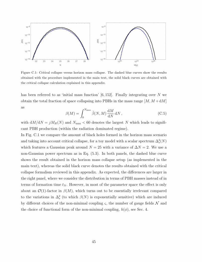
22 23 24 25 26 27 2810-16
10-14
10-12
10-10
10-8
N
β(N
)
1020 1023 102610-16
10-14
10-12
10-10
10-8
M[g]
β(M
)
Figure C.1: Critical collapse versus horizon mass collapse. The dashed blue curves show the results
obtained with the procedure implemented in the main text, the solid black curves are obtained with
the critical collapse calculation explained in this appendix.
has been referred to as ‘initial mass function’ [6, 152]. Finally integrating over N we
obtain the total fraction of space collapsing into PBHs in the mass range [M,M + dM ]
as
β(M) =
∫ Nmax
0
β(N,M)dM
dNdN , (C.5)
with dM/dN = jMH(N) and Nmax < 60 denotes the largest N which leads to signifi-
cant PBH production (within the radiation dominated regime).
In Fig. C.1 we compare the amount of black holes formed in the horizon mass scenario
and taking into account critical collapse, for a toy model with a scalar spectrum ∆2s(N)
which features a Gaussian peak around N = 25 with a variance of ∆N = 2. We use a
non-Gaussian power spectrum as in Eq. (5.3). In both panels, the dashed blue curve
shows the result obtained in the horizon mass collapse setup (as implemented in the
main text), whereas the solid black curve denotes the results obtained with the critical
collapse formalism reviewed in this appendix. As expected, the differences are larger in
the right panel, where we consider the distribution in terms of PBH masses instead of in
terms of formation time tN . However, in most of the parameter space the effect is only
about an O(1)-factor in β(M), which turns out to be essentially irrelevant compared
to the variations in ∆2s (to which β(N) is exponentially sensitive) which are induced
by different choices of the non-minimal coupling ς, the number of gauge fields N and
the choice of functional form of the non-minimal coupling, h(φ), see Sec. 4.
45

Non-spherical collapse
In general, the fluctuations entering the horizon will not be exactly spherical, which
can significantly alter the predictions of PBH formation. As detailed in Ref. [153], the
shape of the mass function is expected to remain essentially the same, but there can
be an overall decrease in the amplitude. We note that in our context this effect is
essentially degenerate with the number of gauge fields in the model, i.e. we expect that
taking into account the ellipticity of the fluctuations might allow us to reproduce the
mass distributions discussed in the main text with a smaller number N of gauge fields.
Mergers and accretion
So far, we have considered primordial black holes as essentially isolated objects. While
this picture is quite appropriate in the radiation dominated regime (where most of the
PBH formation takes place), things become more complicated with the onset of the
matter dominated regime. Due to the slower expansion rate of the universe, clustering
of matter becomes efficient and black holes begin to grow due to the accretion matter
and due to mergers with other PBHs. These processes stabilize the PBHs against decay
through Hawking radiation (an isolated PBH will have decayed by today if M∗ . 5 ·1014 g, whereas the corresponding value at matter radiation equality is M eq
∗ ' 3·1012 g).
It has thus been argued [25], that the overall effect of the merging process may be
estimated by considering all PBHs with a mass heavier than M eq∗ as stable and by
applying an overall shift M → 103M to obtain the mass function today from the mass
function at matter radiation equality. This moreover implies that the fraction of dark
matter consisting of PBHs remains unchanged after the onset of the matter dominated
regime.
In our analysis of the model determined by Eq. (4.9) (which is the only model giving
a significant PBH dark matter contribution), the total amount of PBH dark matter is
rather insensitive to these uncertainties, since our mass distributions are only significant
for M M∗. Furthermore, we note that shifting the mass distribution even by three
orders in magnitude in e.g. Fig. 5.2, will not significantly alter the compatibility of
the spectrum with the existing bounds. This is simply due to the scale invariance of
the bounds over wide ranges of the parameter space. Note however that this discussion
does become relevant when comparing to the mass distribution of PBH observed e.g. by
the LIGO/VIRGO collaboration. Given a peak-like structure in the BH distribution,
46

extracting parameter values in the context of the scenario presented here will require
a more careful study of this question.
References
[1] B. P. Abbott et al. [LIGO Scientific and Virgo Collaborations], Phys. Rev. Lett.
116 (2016) no.6, 061102, [arXiv:1602.03837 [gr-qc]].
[2] K. Danzmann et al., Laser Interferometer Space Antenna (LISA), L3 mission
proposal.
[3] S. Bird, I. Cholis, J. B. Munoz, Y. Ali-Haımoud, M. Kamionkowski,
E. D. Kovetz, A. Raccanelli and A. G. Riess, Phys. Rev. Lett. 116 (2016) no.20,
201301, [arXiv:1603.00464 [astro-ph.CO]].
[4] S. Clesse and J. Garcıa-Bellido, Phys. Dark Univ. 10 (2016) 002,
[arXiv:1603.05234 [astro-ph.CO]].
[5] M. Sasaki, T. Suyama, T. Tanaka and S. Yokoyama, Phys. Rev. Lett. 117 (2016)
no.6, 061101, [arXiv:1603.08338 [astro-ph.CO]].
[6] B. Carr, F. Kuhnel and M. Sandstad, Phys. Rev. D 94 (2016) no.8, 083504,
[arXiv:1607.06077 [astro-ph.CO]].
[7] S. Clesse and J. Garcıa-Bellido, arXiv:1610.08479 [astro-ph.CO].
[8] S. Blinnikov, A. Dolgov, N. K. Porayko and K. Postnov, JCAP 1611 (2016)
no.11, 036 [arXiv:1611.00541 [astro-ph.HE]].
[9] J. Garcıa-Bellido, arXiv:1702.08275 [astro-ph.CO].
[10] J. Georg and S. Watson, arXiv:1703.04825 [astro-ph.CO].
[11] E. Cotner and A. Kusenko, arXiv:1612.02529 [astro-ph.CO].
[12] H. Davoudiasl and P. P. Giardino, Phys. Lett. B 768 (2017) 198,
[arXiv:1609.00907 [gr-qc]].
[13] B. J. Carr, K. Kohri, Y. Sendouda and J. Yokoyama, Phys. Rev. D 81 (2010)
104019, [arXiv:0912.5297 [astro-ph.CO]].
47
[14] J. Garcıa-Bellido, A. D. Linde and D. Wands, Phys. Rev. D 54 (1996) 6040,
[astro-ph/9605094].
[15] D. H. Lyth, arXiv:1107.1681 [astro-ph.CO].
[16] E. Bugaev and P. Klimai, Phys. Rev. D 85 (2012) 103504, [arXiv:1112.5601
[astro-ph.CO]].
[17] S. Clesse and J. Garcıa-Bellido, Phys. Rev. D 92 (2015) no.2, 023524,
[arXiv:1501.07565 [astro-ph.CO]].
[18] K. Kohri, C. M. Lin and T. Matsuda, Phys. Rev. D 87 (2013) no.10, 103527,
[arXiv:1211.2371 [hep-ph]].
[19] M. Kawasaki, N. Kitajima and T. T. Yanagida, Phys. Rev. D 87 (2013) no.6,
063519, [arXiv:1207.2550 [hep-ph]].
[20] E. V. Bugaev and P. A. Klimai, Int. J. Mod. Phys. D 22 (2013) 1350034,
[arXiv:1303.3146 [astro-ph.CO]].
[21] K. Inomata, M. Kawasaki, K. Mukaida, Y. Tada and T. T. Yanagida,
arXiv:1701.02544 [astro-ph.CO].
[22] K. Inomata, M. Kawasaki, K. Mukaida, Y. Tada and T. T. Yanagida,
arXiv:1611.06130 [astro-ph.CO].
[23] M. Kawasaki, A. Kusenko, Y. Tada and T. T. Yanagida, Phys. Rev. D 94 (2016)
no.8, 083523 [arXiv:1606.07631 [astro-ph.CO]].
[24] S. L. Cheng, W. Lee and K. W. Ng, JHEP 1702 (2017) 008 [arXiv:1606.00206
[astro-ph.CO]].
[25] J. Garcıa-Bellido and E. Ruiz Morales, arXiv:1702.03901 [astro-ph.CO].
[26] J. Garcıa-Bellido, M. Peloso and C. Unal, JCAP 1612 (2016) no.12, 031
[arXiv:1610.03763 [astro-ph.CO]].
[27] P. Svrcek and E. Witten, JHEP 0606 (2006) 051 [hep-th/0605206].
[28] M. S. Turner and L. M. Widrow, Phys. Rev. D 37 (1988) 2743.
48
[29] W. D. Garretson, G. B. Field and S. M. Carroll, Phys. Rev. D 46 (1992) 5346
[hep-ph/9209238].
[30] M. M. Anber and L. Sorbo, JCAP 0610 (2006) 018 [astro-ph/0606534].
[31] N. Barnaby, E. Pajer and M. Peloso, Phys. Rev. D 85 (2012) 023525
[arXiv:1110.3327 [astro-ph.CO]].
[32] N. Barnaby and M. Peloso, Phys. Rev. Lett. 106 (2011) 181301 [arXiv:1011.1500
[hep-ph]].
[33] A. Linde, S. Mooij and E. Pajer, Phys. Rev. D 87 (2013) no.10, 103506
[arXiv:1212.1693 [hep-th]].
[34] C. M. Lin and K. W. Ng, Phys. Lett. B 718 (2013) 1181 [arXiv:1206.1685
[hep-ph]].
[35] P. D. Meerburg and E. Pajer, JCAP 1302 (2013) 017 [arXiv:1203.6076
[astro-ph.CO]].
[36] E. Bugaev and P. Klimai, Phys. Rev. D 90 (2014) no.10, 103501
[arXiv:1312.7435 [astro-ph.CO]].
[37] J. L. Cook and L. Sorbo, Phys. Rev. D 85 (2012) 023534 Erratum: [Phys. Rev.
D 86 (2012) 069901] [arXiv:1109.0022 [astro-ph.CO]].
[38] M. M. Anber and L. Sorbo, Phys. Rev. D 85 (2012) 123537 [arXiv:1203.5849
[astro-ph.CO]].
[39] N. Bartolo et al., JCAP 1612 (2016) no.12, 026 [arXiv:1610.06481 [astro-ph.CO]].
[40] V. Domcke, M. Pieroni and P. Binetruy, JCAP 1606 (2016) 031
[arXiv:1603.01287 [astro-ph.CO]].
[41] R. Kallosh, L. Kofman, A. D. Linde and A. Van Proeyen, Class. Quant. Grav. 17
(2000) 4269 Erratum: [Class. Quant. Grav. 21 (2004) 5017] [hep-th/0006179].
[42] F. L. Bezrukov and M. Shaposhnikov, Phys. Lett. B 659 (2008) 703
[arXiv:0710.3755 [hep-th]].
[43] R. Kallosh and A. Linde, JCAP 1307 (2013) 002 [arXiv:1306.5220 [hep-th]].
49

[44] R. Kallosh, A. Linde and D. Roest, Phys. Rev. Lett. 112 (2014) no.1, 011303
[arXiv:1310.3950 [hep-th]].
[45] S. Ferrara, R. Kallosh, A. Linde and M. Porrati, Phys. Rev. D 88 (2013) no.8,
085038 [arXiv:1307.7696 [hep-th]].
[46] M. Galante, R. Kallosh, A. Linde and D. Roest, Phys. Rev. Lett. 114 (2015)
no.14, 141302 [arXiv:1412.3797 [hep-th]].
[47] B. J. Broy, M. Galante, D. Roest and A. Westphal, JHEP 1512 (2015) 149
[arXiv:1507.02277 [hep-th]].
[48] K. Das, V. Domcke and K. Dutta, JCAP 1703 (2017) no.03, 036
[arXiv:1612.07075 [hep-ph]].
[49] R. Kallosh, A. Linde and D. Roest, JHEP 1311 (2013) 198 [arXiv:1311.0472
[hep-th]].
[50] M. B. Einhorn and D. R. T. Jones, JHEP 1003 (2010) 026 [arXiv:0912.2718
[hep-ph]].
[51] S. Ferrara, R. Kallosh, A. Linde, A. Marrani and A. Van Proeyen, Phys. Rev. D
82 (2010) 045003 [arXiv:1004.0712 [hep-th]].
[52] W. Buchmuller, V. Domcke and K. Kamada, Phys. Lett. B 726 (2013) 467
[arXiv:1306.3471 [hep-th]].
[53] G. F. Giudice and H. M. Lee, Phys. Lett. B 733 (2014) 58 [arXiv:1402.2129
[hep-ph]].
[54] C. Pallis, JCAP 1404 (2014) 024 [arXiv:1312.3623 [hep-ph]].
[55] C. Pallis, JCAP 1408 (2014) 057 [arXiv:1403.5486 [hep-ph]].
[56] C. Pallis, JCAP 1410 (2014) no.10, 058 [arXiv:1407.8522 [hep-ph]].
[57] J. Ellis, D. V. Nanopoulos and K. A. Olive, Phys. Rev. Lett. 111 (2013) 111301
Erratum: [Phys. Rev. Lett. 111 (2013) no.12, 129902] [arXiv:1305.1247 [hep-th]].
[58] R. Kallosh and A. Linde, JCAP 1306 (2013) 028 [arXiv:1306.3214 [hep-th]].
50

[59] K. Nakayama and F. Takahashi, JCAP 1011 (2010) 039 [arXiv:1009.3399
[hep-ph]].
[60] M. Pieroni, JCAP 1602 (2016) no.02, 012 [arXiv:1510.03691 [hep-ph]].
[61] P. A. R. Ade et al. [Planck Collaboration], Astron. Astrophys. 594 (2016) A20
[arXiv:1502.02114 [astro-ph.CO]].
[62] M. M. Anber and L. Sorbo, Phys. Rev. D 81 (2010) 043534 [arXiv:0908.4089
[hep-th]].
[63] N. Barnaby, R. Namba and M. Peloso, JCAP 1104 (2011) 009 [arXiv:1102.4333
[astro-ph.CO]].
[64] K. Freese, J. A. Frieman and A. V. Olinto, Phys. Rev. Lett. 65 (1990) 3233.
[65] M. Pieroni, arXiv:1611.03732 [gr-qc].
[66] P. A. R. Ade et al. [Planck Collaboration], Astron. Astrophys. 594 (2016) A17
[arXiv:1502.01592 [astro-ph.CO]].
[67] M. Maggiore, “Gravitational Waves. Vol. 1: Theory and Experiments,” Oxford
University Press (2007).
[68] S. G. Crowder, R. Namba, V. Mandic, S. Mukohyama and M. Peloso, Phys. Lett.
B 726 (2013) 66 [arXiv:1212.4165 [astro-ph.CO]].
[69] N. D. Birrell and P. C. W. Davies, “Quantum Fields in Curved Space”,
Cambridge Monographs on Mathematical Physics (1984).
[70] F. Bezrukov and M. Shaposhnikov, JHEP 0907 (2009) 089 [arXiv:0904.1537
[hep-ph]].
[71] D. I. Kaiser and E. I. Sfakianakis, Phys. Rev. Lett. 112 (2014) no.1, 011302
[arXiv:1304.0363 [astro-ph.CO]].
[72] R. Kallosh and A. Linde, JCAP 1312 (2013) 006 [arXiv:1309.2015 [hep-th]].
[73] R. Kallosh, A. Linde and D. Roest, JHEP 1408 (2014) 052 [arXiv:1405.3646
[hep-th]].
51

[74] R. Kallosh and A. Linde, Phys. Rev. D 91 (2015) 083528 [arXiv:1502.07733
[astro-ph.CO]].
[75] P. A. R. Ade et al. [Planck Collaboration], Astron. Astrophys. 594 (2016) A13
[arXiv:1502.01589 [astro-ph.CO]].
[76] V. Mukhanov, Eur. Phys. J. C 73 (2013) 2486 [arXiv:1303.3925 [astro-ph.CO]].
[77] D. Roest, JCAP 1401 (2014) 007 [arXiv:1309.1285 [hep-th]].
[78] P. Binetruy, E. Kiritsis, J. Mabillard, M. Pieroni and C. Rosset, JCAP 1504
(2015) no.04, 033 [arXiv:1407.0820 [astro-ph.CO]].
[79] A. A. Starobinsky, Phys. Lett. 91B (1980) 99.
[80] T. L. Smith, M. Kamionkowski and A. Cooray, Phys. Rev. D 73 (2006) 023504
[astro-ph/0506422].
[81] R. van Haasteren et al., Mon. Not. Roy. Astron. Soc. 414 (2011) no.4, 3117
Erratum: [Mon. Not. Roy. Astron. Soc. 425 (2012) no.2, 1597] [arXiv:1103.0576
[astro-ph.CO]].
[82] M. Kramer, “Fundamental physics with the SKA: Strong-field tests of gravity
using pulsars and black holes,” astro-ph/0409020.
[83] A. Petiteau, in preparation.
[84] C. Caprini et al., JCAP 1604 (2016) no.04, 001 [arXiv:1512.06239 [astro-ph.CO]].
[85] B. P. Abbott et al. [LIGO Scientific and Virgo Collaborations], Phys. Rev. Lett.
116 (2016) no.13, 131102 [arXiv:1602.03847 [gr-qc]].
[86] M. Peloso, L. Sorbo and C. Unal, JCAP 1609 (2016) no.09, 001
[arXiv:1606.00459 [astro-ph.CO]].
[87] A. M. Green, A. R. Liddle, K. A. Malik and M. Sasaki, Phys. Rev. D 70 (2004)
041502 [astro-ph/0403181].
[88] P. Pina Avelino, Phys. Rev. D 72 (2005) 124004
doi:10.1103/PhysRevD.72.124004 [astro-ph/0510052].
52

[89] D. H. Lyth, JCAP 1205 (2012) 022 doi:10.1088/1475-7516/2012/05/022
[arXiv:1201.4312 [astro-ph.CO]].
[90] C. T. Byrnes, E. J. Copeland and A. M. Green, Phys. Rev. D 86, 043512 (2012)
[arXiv:1206.4188 [astro-ph.CO]].
[91] F. Capela, M. Pshirkov and P. Tinyakov, Phys. Rev. D 87 (2013) no.12, 123524
[arXiv:1301.4984 [astro-ph.CO]].
[92] K. Griest, A. M. Cieplak and M. J. Lehner, Astrophys. J. 786 (2014) no.2, 158
[arXiv:1307.5798 [astro-ph.CO]].
[93] P. Tisserand et al. [EROS-2 Collaboration], Astron. Astrophys. 469 (2007) 387
[astro-ph/0607207].
[94] S. Calchi Novati, S. Mirzoyan, P. Jetzer and G. Scarpetta, Mon. Not. Roy.
Astron. Soc. 435 (2013) 1582 [arXiv:1308.4281 [astro-ph.GA]].
[95] H. Niikura et al., arXiv:1701.02151 [astro-ph.CO].
[96] B. P. Abbott et al. [LIGO Scientific and Virgo Collaborations], Phys. Rev. Lett.
116 (2016) no.13, 131103 [arXiv:1602.03838 [gr-qc]].
[97] C. W. Misner, K. S. Thorne and J. A. Wheeler, San Francisco 1973, 1279p.
[98] P. Adshead, J. T. Giblin, T. R. Scully and E. I. Sfakianakis, JCAP 1512 (2015)
no.12, 034 [arXiv:1502.06506 [astro-ph.CO]].
[99] A. Kusenko, K. Schmitz and T. T. Yanagida, Phys. Rev. Lett. 115 (2015) no.1,
011302 [arXiv:1412.2043 [hep-ph]].
[100] M. M. Anber and E. Sabancilar, Phys. Rev. D 92 (2015) no.10, 101501
[arXiv:1507.00744 [hep-th]].
[101] P. Adshead and E. I. Sfakianakis, Phys. Rev. Lett. 116 (2016) no.9, 091301
[arXiv:1508.00881 [hep-ph]].
[102] R. J. Crewther, P. Di Vecchia, G. Veneziano and E. Witten, Phys. Lett. 88B
(1979) 123 Erratum: [Phys. Lett. 91B (1980) 487].
[103] C. A. Baker et al., Phys. Rev. Lett. 97 (2006) 131801 [hep-ex/0602020].
53
[104] R. D. Peccei and H. R. Quinn, Phys. Rev. Lett. 38 (1977) 1440.
[105] F. Wilczek, Phys. Rev. Lett. 40 (1978) 279.
[106] S. Weinberg, Phys. Rev. Lett. 40 (1978) 223.
[107] C. Vafa and E. Witten, Phys. Rev. Lett. 53 (1984) 535.
[108] P. Anastasopoulos, M. Bianchi, E. Dudas and E. Kiritsis, JHEP 0611 (2006)
057 [hep-th/0605225].
[109] G. Dvali, hep-th/0507215.
[110] N. Kaloper and L. Sorbo, Phys. Rev. Lett. 102 (2009) 121301 [arXiv:0811.1989
[hep-th]].
[111] N. Kaloper, A. Lawrence and L. Sorbo, JCAP 1103 (2011) 023
[arXiv:1101.0026 [hep-th]].
[112] N. Arkani-Hamed, L. Motl, A. Nicolis and C. Vafa, JHEP 0706 (2007) 060
[hep-th/0601001].
[113] J. P. Conlon, JCAP 1209 (2012) 019 [arXiv:1203.5476 [hep-th]].
[114] F. Marchesano, G. Shiu and A. M. Uranga, JHEP 1409 (2014) 184
[arXiv:1404.3040 [hep-th]].
[115] R. Blumenhagen and E. Plauschinn, Phys. Lett. B 736 (2014) 482
[arXiv:1404.3542 [hep-th]].
[116] A. Hebecker, S. C. Kraus and L. T. Witkowski, Phys. Lett. B 737 (2014) 16
[arXiv:1404.3711 [hep-th]].
[117] S. Ferrara, R. Kallosh, A. Linde, A. Marrani and A. Van Proeyen, Phys. Rev. D
83 (2011) 025008 [arXiv:1008.2942 [hep-th]].
[118] W. Buchmuller, V. Domcke and K. Schmitz, JCAP 1304 (2013) 019
[arXiv:1210.4105 [hep-ph]].
[119] M. K. Gaillard and V. Jain, Phys. Rev. D 49 (1994) 1951 [hep-th/9308090].
[120] E. D. Stewart, Phys. Lett. B 391 (1997) 34 [hep-ph/9606241].
54
[121] E. D. Stewart, Phys. Rev. D 56 (1997) 2019 [hep-ph/9703232].
[122] D. Baumann and L. McAllister, arXiv:1404.2601 [hep-th].
[123] A. Arvanitaki, S. Dimopoulos, S. Dubovsky, N. Kaloper and J. March-Russell,
Phys. Rev. D 81 (2010) 123530 [arXiv:0905.4720 [hep-th]].
[124] M. Cicoli, M. Goodsell and A. Ringwald, JHEP 1210 (2012) 146
[arXiv:1206.0819 [hep-th]].
[125] A. Westphal, Int. J. Mod. Phys. A 30 (2015) no.09, 1530024 [arXiv:1409.5350
[hep-th]].
[126] J. E. Kim, H. P. Nilles and M. Peloso, JCAP 0501 (2005) 005 [hep-ph/0409138].
[127] T. C. Bachlechner, M. Dias, J. Frazer and L. McAllister, Phys. Rev. D 91
(2015) no.2, 023520 [arXiv:1404.7496 [hep-th]].
[128] G. Shiu, W. Staessens and F. Ye, JHEP 1506 (2015) 026 [arXiv:1503.02965
[hep-th]].
[129] S. Dimopoulos, S. Kachru, J. McGreevy and J. G. Wacker, JCAP 0808 (2008)
003 [hep-th/0507205].
[130] M. Cicoli, K. Dutta and A. Maharana, JCAP 1408 (2014) 012 [arXiv:1401.2579
[hep-th]].
[131] K. Das and K. Dutta, Phys. Lett. B 738 (2014) 457 [arXiv:1408.6376 [hep-ph]].
[132] E. Silverstein and A. Westphal, Phys. Rev. D 78 (2008) 106003
[arXiv:0803.3085 [hep-th]].
[133] L. McAllister, E. Silverstein and A. Westphal, Phys. Rev. D 82 (2010) 046003
[arXiv:0808.0706 [hep-th]].
[134] T. Rudelius, JCAP 1509 (2015) no.09, 020 [arXiv:1503.00795 [hep-th]].
[135] B. Heidenreich, M. Reece and T. Rudelius, JHEP 1512 (2015) 108
[arXiv:1506.03447 [hep-th]].
[136] M. Cicoli, C. P. Burgess and F. Quevedo, JCAP 0903 (2009) 013
[arXiv:0808.0691 [hep-th]].
55

[137] C. P. Burgess, M. Cicoli, S. de Alwis and F. Quevedo, JCAP 1605 (2016)
no.05, 032 [arXiv:1603.06789 [hep-th]].
[138] M. Cicoli, D. Ciupke, S. de Alwis and F. Muia, JHEP 1609 (2016) 026
[arXiv:1607.01395 [hep-th]].
[139] M. Cicoli, F. Muia and P. Shukla, JHEP 1611 (2016) 182 [arXiv:1611.04612
[hep-th]].
[140] M. Cicoli, D. Ciupke, V. A. Diaz, V. Guidetti, F. Muia and P. Shukla, in
preparation.
[141] X. Dong, B. Horn, E. Silverstein and A. Westphal, Phys. Rev. D 84 (2011)
026011 [arXiv:1011.4521 [hep-th]].
[142] L. McAllister, E. Silverstein, A. Westphal and T. Wrase, JHEP 1409 (2014)
123 [arXiv:1405.3652 [hep-th]].
[143] J. P. Conlon and E. Palti, JHEP 0909 (2009) 019 [arXiv:0906.1920 [hep-th]].
[144] M. W. Choptuik, Phys. Rev. Lett. 70 (1993) 9.
[145] T. Koike, T. Hara and S. Adachi, Phys. Rev. Lett. 74 (1995) 5170
[gr-qc/9503007].
[146] J. C. Niemeyer and K. Jedamzik, Phys. Rev. D 59 (1999) 124013
[astro-ph/9901292].
[147] C. Gundlach, Living Rev. Rel. 2 (1999) 4 [gr-qc/0001046].
[148] C. Gundlach, Phys. Rept. 376 (2003) 339 [gr-qc/0210101].
[149] I. Musco, J. C. Miller and L. Rezzolla, Class. Quant. Grav. 22 (2005) 1405
[gr-qc/0412063].
[150] I. Musco, J. C. Miller and A. G. Polnarev, Class. Quant. Grav. 26 (2009)
235001 [arXiv:0811.1452 [gr-qc]].
[151] I. Musco and J. C. Miller, Class. Quant. Grav. 30 (2013) 145009
[arXiv:1201.2379 [gr-qc]].
56

[152] J. C. Niemeyer and K. Jedamzik, Phys. Rev. Lett. 80 (1998) 5481
[astro-ph/9709072].
[153] F. Kuhnel and M. Sandstad, Phys. Rev. D 94 (2016) no.6, 063514
[arXiv:1602.04815 [astro-ph.CO]].
57