paying more for a shorter flight? - hidden city ticketing

Paying More for a Shorter Flight? - Hidden City

Ticketing

Quanquan LiuDepartment of Economics, University of Pittsburgh, Pittsburgh, PA 15260, USA

Hidden city ticketing occurs when an indirect flight from city A to city C through connection node city

B is cheaper than the direct flight from city A to city B. Then passengers traveling from A to B have an

incentive to purchase the ticket from A to C but get off the plane at B. In this paper, I build a structural

model to explain the cause and impact of hidden city ticketing. I collect empirical data from the Skiplagged

webpage and apply global optimization algorithms to estimate the parameters of my model. I also conduct

counterfactual analysis to shed some light on policy implications. I find that hidden city opportunity occurs

only when airlines are applying a hub-and-spoke network structure, under which they intend to lower their

flying costs compared to a fully connected network. I find that in the short run, hidden city ticketing does

not necessarily decrease airlines’ expected profits. Consumer welfare and total surplus always increase. In

the long run, the welfare outcomes become more complicated. For some routes airlines have the incentive

to switch from hub-and-spoke network to a fully connected one when there are more and more passengers

informed of hidden city ticketing. During this process, firms always result in lower expected profits, while

consumers and the whole society are not necessarily better off.

Keywords: hidden city ticketing, network structure, second-degree price discrimination, informed con-

sumers.

1. Introduction

Hidden city ticketing is an interesting pricing phenomenon occurring after the deregulation of the

airline industry in 1978 (Wang & Ye (2016)). It is an airline booking strategy passengers use to

reduce their flying costs. Hidden city ticketing occurs when an indirect flight from city A to city

C, using city B as the connection node, turns out to be cheaper than the direct flight from city

A to city B. In which case passengers who wish to fly from A to B have an incentive to purchase

the indirect flight ticket, pretend to fly to city C, while disembark at the connection node B, and

discard the remaining segment B to C. When this happens, city B is called the “hidden city”, and

this behavior is then called “hidden city ticketing”.

The following real world example (Figure 1) illustrates hidden city ticketing. On November 19,

2018, a direct flight operated by Delta Air Lines flying from Pittsburgh to New York city cost $218.

On the same day, for the same departure and landing time, another indirect flight also operated

1

Liu: Hidden City Ticketing 2

Figure 1 An example of hidden city ticketing.

by Delta Air Lines flying from Pittsburgh to Boston, with one stop at New York city, cost only

$67.

These two flights share exactly the same first segment: they are operated by the same airline

company, they departure at the same date, same airports and same time. However, the price of

the indirect flight accounted for only 30% of that of the direct one. That is, you are able to fly

more than 200 miles further but pay $151 less! The New York city is then called a “hidden city”

in this case. It is “hidden” because literally, if we use Google Flights, Orbitz, Priceline, Kayak, or

any other “normal” travel search tools to look for a flight from Pittsburgh to NYC, we will not be

able to see the indirect flight above showing up in our search results.

Although technically legal, hidden city ticketing actually violates the airfare rules of most airline

companies in United States. For example, according to the Contract of Carriage of United Airlines

(revised by December 31, 2015):

“Fares apply for travel only between the points for which they are published. Tickets may not

be purchased and used at fare(s) from an initial departure point on the Ticket which is before the

Passenger’s actual point of origin of travel, or to a more distant point(s) than the Passenger’s

actual destination being traveled even when the purchase and use of such Tickets would produce a

lower fare. This practice is known as “Hidden Cities Ticketing” or “Point Beyond Ticketing” and

is prohibited by UA.”

Similarly, American Airlines also claim that conducting hidden city ticketing is “unethical” and

doing so “is tantamount to switching price tags to obtain a lower price on goods sold at department

stores”. Passengers might be penalized when conducting hidden city ticketing. Airlines are able to

“confiscate any unused Flight Coupons”, “delete miles in the passenger’s frequent flyer account”,

“assess the passenger for the actual value of the ticket”, or even “take legal action with respect to

the passenger”.


Meanwhile, members of Congress have proposed several bills, including “H.R. 700, H.R. 2200,

H.R. 5347 and S. 2891, H.R. 332, H.R. 384, H.R. 907 and H.R. 1074”, trying to prohibit airlines

from penalizing passengers for conducting hidden city ticketing (GAO (2001)). Furthermore, the

European Union has passed a passenger bill of rights since around 2005, in which the European

Commission has specifically ruled that “airlines must honor any part of an airline ticket” and

hidden city ticketing then becomes perfectly legal. After the ruling EU find that “fares have become

more fair, hidden city bargains are difficult to find, and the airlines have not suffered drastic losses

due to this”.

Therefore, whether hidden city ticketing should be legally prohibited or not, and what policy

does the best for consumers, airline companies, and social welfare, still remain to be open questions.

The fact is, although being “threatened” by airline companies, there have been more and more

consumers coming to realize the existence of hidden city opportunities, and may try to exploit

them to lower their flying costs. In December 2014, United Airlines and Orbitz (an airline booking

platform) sued the founder of Skiplagged (a travel search tool) for his website of “helping travelers

find cheap tickets through hidden city ticketing”. According to CNNMoney, Orbitz eventually

settled out of court one year later, and a Chicago judge threw out United’s lawsuit using the excuse

that the founder “did not live or do business in that city”. In contrast to the willingness of United,

this lawsuit brought the search of key words “hidden city ticketing” to a peak (Figure 2).

Corresponding to this higher demand, nowadays there are more travel search tools specifically

designed to achieve this task (Skiplagged, Tripdelta, Fly Shortcut, AirFareIQ, ITA Matrix, etc).

And finding hidden city opportunies and exploiting them become much easier today.

This paper aims at providing some plausible explanations for the cause of hidden city ticketing,

and estimating its possible impact on welfare outcomes for airlines, consumers, and society as a

whole. I build a structural model in which airlines can choose both prices and network structures as

their strategic variables following Shy (2001), and derive several propositions based on that. Then

I collect daily flights information by scraping the Skiplagged website to build my own empirical

dataset. I apply global optimization algorithms to estimate the parameters of my model, and then

conduct counterfactual analysis to evaluate the possible impact of hidden city ticketing on airlines’

expected profits, consumers’ welfare, and total surplus, based on which I could help shed some

light on policy implications.

In this paper, I find that 1) hidden city ticketing only occurs when airline companies are applying

a hub-and-spoke network structure; 2) under some conditions, hub-and-spoke network is more cost-

saving compared to fully connected network; 3) in the short run, hidden city ticketing does not


Figure 2 Average monthly web search data of hidden city ticketing. Data source for the relative value is

Google Trends. Numbers represent search interest relative to the highest point on the chart for the given region

and time. A value of 100 is the peak popularity for the term. Data source for the absolute value is Google

AdWords, unit is number of times.

necessarily decrease airlines’ expected profits, while consumers’ surplus and total welfare always

increase; 4) in the long run, i.e., when airlines can change their choices of prices and networks freely,

the impact of hidden city ticketing differs for different routes. For some routes airlines have the

incentive to switch from hub-and-spoke network to a fully connected one when there are more and

more passengers informed of hidden city ticketing, during which process firms always result in lower

expected revenue, while consumers and the whole society are not necessarily better off. Therefore,

whether hidden city ticketing should be permitted or forbidden depends on the characteristics of

different routes, and this problem cannot be solved by one simple policy.

The remainder of this paper is organized as follows: Related works are summarized in Section 2.

The structural model is introduced in Section 3, together with the propositions of short run impacts

derived from it. Section 4 describes the data in details. Section 5 shows the estimation strategy

and the MLE results. In Section 6 I conduct counterfactual analysis to shed some light on long run

impacts and policy implications. The limitation and future questions of this paper are discussed

in Section 7 and Section 8 concludes.


2. Literature Review

To the best of my knowledge, this is the first paper to quantitatively study the cause and impact

of hidden city ticketing on welfare outcomes using real empirical data. In fact, there are only a

few papers paying attention to this phenomenon. One government report from the Government

Accountability Office (GAO (2001)) conducted some correlation analysis based on their selected

data, and found that the possibility of hidden city ticketing is significantly affected by the size of the

markets and the degree of competition in the hub markets and the spoke markets. Another report

from Hopper Research (Surry (2005)) also provides some summary statistics of this phenomenon.

Based on four weeks of airfare search data from Hopper, the analyst found that 26% of domestic

routes could be substituted by some cheaper options through hidden city ticketing, and the price

discount could be nearly 60%. The most quantitative study is Wang & Ye (2016), which applied

a network revenue management model to look at the cause and impact of hidden city ticketing.

They base all their findings on simulated data rather than real world data. Therefore, their model

is quite different from an economic model. They find that hidden city opportunity may arise when

the price elasticity of demand on different routes differ a lot. In order to eliminate any hidden

city opportunities, airlines will rise the prices of certain itineraries and hurt consumers. But even

airlines optimally react, they will still suffer from a loss in revenue.

There have been a lot of literature focusing on the airline industry ever since its deregulation

in 1978. A bunch of them have confirmed significant difference of price elasticity lying between

tourists and business travelers. For example, Berry & Jia (2010) has estimated a price elasticity of

demand for tourists as −6.55, while that for business travelers is only −0.63. Robert S & Daniel L

(2001) find a large difference between price elasticity of demand for business travelers (−0.9 to

−0.3) and that for leisure travelers (about −1.5). And Gerardi & Shapiro (2009) also confirm that

the demand for business travelers is less price elastic than that of tourists, and through applying

certain ticket restrictions, airline companies are able to distinguish between these two types. Based

on these findings, researchers have further found that airlines are exploiting these differences and

engaging in second-degree price discrimination through many different methods, such as advanced-

purchase discounts (Dana (1998)), ticket restrictions such as Saturday-night stayover requirements

(Stavins (2001); Giaume & Guillou (2004)), refundable and non-refundable tickets (Escobari &

Jindapon (2014)), intertemporal price discrimination (Liu (2015); Lazarev (2013)), and even the

day-of-the-week that a ticket is purchased (Puller & Taylor (2012)). This paper follows previous

findings and assumes that airline companies are price discriminating between leisure travelers and

business travelers, with the latter being less price sensitive and valuing time more. My model also

follows Shy (2001) book about economics of network industries, assuming that airlines can choose


Figure 3 Left: Fully-Connected (FC) Network. Right: Hub-and-Spoke (HS) Network.

both airfares and network structures. Finally, I find that while informed passengers could possibly

enjoy some benefits of hidden city ticketing, uninformed passengers are always bearing the costs,

if any. This is similar to the finding of Varian (1980) where the author shows some “detrimental

externalities” that uninformed consumers suffer from due to the behavior of informed consumers.

3. The Model

Following Shy (2001), I assume that airlines are choosing from two different network structures:

fully-connected network or hub-and-spoke network (Figure 3). Under fully-connected network,

passengers fly nonstop from one city to the other. While under hub-and-spoke network, everyone

who wishes to fly from city A to city C needs to stop at the hub city B. To simplify my analysis

below, I will apply an one-way traveling pattern instead of the two-way traveling pattern showed

in Figure 3. After the 1978 Airline Deregulation Act, the absence of price and entry controls

led to increased use of the hub-and-spoke structure (Shy (2001)). Responding to the increased

competition and to reduce flying costs, airlines started to cut the number of direct flights and

reroute the passengers through a hub city. While in recent years, especially since late 1990s, with

the expansion of low-cost carriers (LCCs), passengers started to show a higher aversion toward

connecting flights, and fully-connected structure becomes more popular again (Berry & Jia (2010)).

Assume that there is only one airline serving the three cities, thus the firm charges monopoly

airfares. Aircrafts are further assumed to have an unlimited capacity, thus there is only one flight

on each route. C2 denote the airline’s cost per mile on any route j. This simplified cost pattern

is referred as ACM cost (AirCraft Movement cost) in Shy (2001), and it is widely used in airline

related literature. Cost pattern can be simplified because in airline industry, large percentage of

costs are fixed before flights taking off, such as capital costs (renting gates for departure and

arrival, landing fees), labor costs (hiring local staff), etc. (GAO (2001)) The costs of fuel account

for approximately 15% of the total operation costs (Berry & Jia (2010)), while the marginal cost

of airline seats is nearly negligible (Rao (2009)).


Assume that direct flight has a quality of qh per mile and indirect flight has a quality of ql per

mile, with 0< ql < qh < 1. Each individual i has a time preference parameter of λi, obtaining utility

ui =C1 · eλiqd− p

from consuming a good of quality q. Under the assumption of free disposal, he/she will get 0 utility

if chooses not to fly. Utility decreases when price increases. And if a passenger values time more

(i.e., with a larger λ), he/she will acquire a larger utility increase when switching from an indirect

flight (with quality ql) to a direct flight (with quality qh). Furthermore, for a longer itinerary

(larger d), the utility improvement from indirect flight to direct flight is also larger. C1 is a scaling

parameter to make the utility comparable to dollar value p.

On each route j, the distribution of consumers’ time preferences satisfies λij ∼ N(θj, σ21). For

passengers flying from A to B, the fraction of passengers being aware of hidden city opportunities

is δ, and the fraction of uninformed passengers is 1− δ. When hidden city opportunities exist (i.e.,

pAB > pABC), informed passengers will pay pABC instead, while uninformed passengers will still

pay pAB. The amount of passengers on each route j are normalized to 1. pj denote the airfare on

route j, and dj denote the distance of route j.

Airline chooses both network structures (fully-connected or hub-and-spoke) and prices

(pAB, pBC , pAC , pABC) to maximize expected profits, as shown in the figure below.

Airline

ΠFC(pFC)

pFC = (pAB, pBC , pAC)

Fully-Connected

ΠHS(pHS)

pHS = (pAB, pBC , pABC)

Hub-and-Spoke

I will show later in this section that there exists an optimal choice set for the airline, and the

choice set is unique. According to the assumptions above, on each route j, for each individual i,

uij =C1 · eλijqd− p, λij ∼N(θj, σ21).

Therefore, on each route j, the proportion of consumers choosing to fly is equal to:

Pr [uij ≥ 0] = Pr[C1 · eλijqd≥ p

]


= Pr

[λij ≥ ln

(p

C1 · qd

)]= 1−Φθj ,σ

21

(ln

(p

C1 · qd

)).

3.1. Fully-Connected Network

Under fully-connected network, airline’s expected profits (producer surplus) are equal to the rev-

enue it collects minus the costs:

ΠFC = ΠAB + ΠBC + ΠAC

= pAB ·[1−ΦθAB ,σ

21

(ln

(pAB

C1 · qhdAB

))]−C2 · dAB

+ pBC ·[1−ΦθBC ,σ

21

(ln

(pBC

C1 · qhdBC

))]−C2 · dBC

+ pAC ·[1−ΦθAC ,σ

21

(ln

(pAC

C1 · qhdAC

))]−C2 · dAC .

Under fully-connected network structure, the only way to fly “indirectly” from A to C is to take

the two direct flights A to B and B to C together. Obviously, with pAB < pAB +pBC , we can easily

derive the following proposition:

Proposition 1 Hidden city opportunity does not exist under fully-connected network structure.

Consumer surplus is the difference between our willingness to pay and the price we actually

being charged, which equals:

CSFC = CSAB +CSBC +CSAC

=

∫ ∞ln

( pABC1 · qhdAB

) (C1 · eλiqhdAB − pAB)dF (λi)

+

∫ ∞ln

( pBCC1 · qhdBC

) (C1 · eλiqhdBC − pBC)dF (λi)

+

∫ ∞ln

( pACC1 · qhdAC

) (C1 · eλiqhdAC − pAC)dF (λi).

Adding them together, our total surplus under fully-connected network is:

TSFC = PSFC +CSFC

=

∫ ∞ln

( pABC1 · qhdAB

) (C1 · eλiqhdAB)dF (λi)−C2 · dAB


+

∫ ∞ln

( pBCC1 · qhdBC

) (C1 · eλiqhdBC)dF (λi)−C2 · dBC

+

∫ ∞ln

( pACC1 · qhdAC

) (C1 · eλiqhdAC)dF (λi)−C2 · dAC .

No transaction fee is assumed under the setting, thus the prices we pay are equal to the prices

airline receives, and both cancel out.

3.2. Hub-and-Spoke Network (without Hidden City Ticketing)

Given hub-and-spoke network structure, first consider the simple case when hidden city opportu-

nities do not exist (i.e., pAB ≤ pABC). Under this circumstances, airline’s expected profits are equal

to:

ΠHS = ΠAB + ΠBC + ΠABC

= pAB ·[1−ΦθAB ,σ

21

(ln

(pAB

C1 · qhdAB

))]−C2 · dAB


21

(ln

(pBC

C1 · qhdBC

))]−C2 · dBC

+ pABC ·[1−ΦθABC ,σ

21

(ln

(pABC

C1 · qldABC

))].

Proposition 2 If the cost associated with maintaining route AC is sufficiently large, then the hub-

and-spoke network is more profitable to operate than the fully-connected network for the monopoly

airline.

Proof of Proposition 2. Compare airline’s expected profits under these two different networks:

ΠHS −ΠFC = pABC ·[1−ΦθABC ,σ

21

(ln

(pABC

C1 · qldABC

))]− pAC ·

[1−ΦθAC ,σ

21

(ln

(pAC

C1 · qhdAC

))]+ C2 · dAC .

Therefore, if the last term (C2 · dAC , refers to the cost associated with maintaining route AC) is

sufficiently large, hub-and-spoke network is more profitable.

This is in accordance with the findings of previous literatures. Caves et al. (1984), Brueckner

et al. (1992), Brueckner & Spiller (1994), and Berry et al. (2006) all confirm the cost economies

of hubbing. Under a different framework, Shy (2001) also find that hub-and-spoke network is cost-

saving if the fixed cost is large enough.


Similarly, consumer surplus equals:

CSHS = CSAB +CSBC +CSABC

=

∫ ∞ln

( pABC1 · qhdAB


+

∫ ∞ln

( pBCC1 · qhdBC


+

∫ ∞ln

( pABCC1 · qldABC

) (C1 · eλiqldABC − pABC)dF (λi).

Adding them together, total surplus is equal to:

TSHS = PSHS +CSHS

=

∫ ∞ln

( pABC1 · qhdAB


+

∫ ∞ln

( pBCC1 · qhdBC


+

∫ ∞ln

( pABCC1 · qldABC

) (C1 · eλiqldABC)dF (λi).

3.3. Hub-and-Spoke Network (with Hidden City Ticketing)

Now consider the scenario when hidden city opportunities exist (i.e., pAB > pABC). Firstly, is there

a possibility that pAB > pABC , in other words, are we paying more for a shorter flight sometimes?

The answer is yes. To see why this might occur, recall that

pAB = argmaxp

p ·[1−ΦθAB ,σ

21

(ln(

p

C1qhdAB)

)],

pABC = argmaxp

p ·[1−ΦθABC ,σ

21

(ln(

p

C1qldABC)

)],

where qh > ql and dAB < dABC . For simplification, let qhdAB = qldABC and σ1 = 1, rewrite the

problem as

p = argmaxp

p ·[1−Φθ

(ln(

p

C))]

= argmaxp

p ·[1−Φ

(ln(

p

C)− θ

)],

where C is a constant.


Let f(p, θ) = p ·[1−Φ

(ln(

p

C)− θ

)], to find out the maximizer p∗, take derivative of f(p, θ) with

respect to p and make it equal 0:

fp(p, θ) = 1−Φ(ln(

p

C)− θ

)−φ

(ln(

p

C)− θ

)= 0.

Let g(p, θ) = 1−Φ(ln(

p

C)− θ

)−φ

(ln(

p

C)− θ

), and take derivative of g(p, θ) with respect to θ,

we get

gθ(p, θ) = φ(ln(

p

C)− θ

)+φθ

(ln(

p

C)− θ

)= φ

(ln(

p

C)− θ

)(1− ln(

p

C) + θ

).

Since φ(ln(

p

C)− θ

)> 0, if θ > ln(

p

C)− 1, we would have gθ(p, θ)> 0, hence as long as θAB >

θABC , the optimal prices would be pAB > pABC . Therefore, under some conditions, there is a pos-

sibility that pAB > pABC , in other words, we are paying more for a shorter flight sometimes and

hidden city opportunities exist. The underlying explanation is that airlines are pricing based on

demand, rather than costs.

Comparing to Section 3.2 where there is no hidden city ticketing, the difference lies in the

informed passengers who wish to fly directly from A to B. Under this circumstances, airline’s

expected profits are equal to:

ΠHCT = ΠAB + ΠBC + ΠABC

= (1− δ) · pAB ·[1−ΦθAB ,σ

21

(ln

(pAB

C1 · qhdAB

))]−C2 · dAB


21

(ln

(pBC

C1 · qhdBC

))]−C2 · dBC


21

(ln

(pABC

C1 · qldABC

))]+ δ · pABC ·

[1−ΦθAB ,σ

21

(ln

(pABC

C1 · qhdAB

))].

Proposition 3 When airlines do not alter their choices of prices and network structures, hidden

city ticketing does not necessarily decrease airline’s expected profits.

Proof of Proposition 3. Compare airline’s expected profits with and without hidden city tick-

eting respectively, and compute the difference:

ΠHCT −ΠHS = δ ·{pABC ·

[1−ΦθAB ,σ

21

(ln

(pABC

C1 · qhdAB

))]


− pAB ·[1−ΦθAB ,σ

21

(ln

(pAB

C1 · qhdAB

))]}.

Note that pABC < pAB while

[1−ΦθAB ,σ

21

(ln

(pABC

C1 · qhdAB

))]>

[1−ΦθAB ,σ

21

(ln

(pAB

C1 · qhdAB

))].

We find that although airline suffers from a loss when informed passengers are paying a lower price,

it also obtains some gain when this lower price attracts more consumers to take the flight. How

hidden city ticketing will affect airline’s expected profits actually depends on the relative dominance

of these two inequalities, and this conduct does not necessarily decrease airline’s expected revenue.

Consumer surplus equals:

CSHCT = CSAB +CSBC +CSABC

= (1− δ)∫ ∞ln

( pABC1 · qhdAB


+

∫ ∞ln

( pBCC1 · qhdBC


+

∫ ∞ln

( pABCC1 · qldABC

) (C1 · eλiqldABC − pABC)dF (λi).

+ δ

∫ ∞ln

( pABCC1 · qhdAB

) (C1 · eλiqhdAB − pABC)dF (λi).

Proposition 4 When airlines do not alter their choices of prices and network structures, con-

sumers are always better off when hidden city ticketing is allowed.

Proof of Proposition 4. Compute the difference of consumer surplus with and without hidden

city ticketing, we have

CSHCT −CSHS = δ

∫ ∞ln

( pABCC1 · qhdAB

) (C1 · eλiqhdAB − pABC)dF (λi)

− δ

∫ ∞ln

( pABC1 · qhdAB


= δ

∫ ln

( pABC1 · qhdAB

)

ln

( pABCC1 · qhdAB

) (C1 · eλiqhdAB − pABC

)dF (λi)

+ δ

∫ ∞ln

( pABC1 · qhdAB

) (pAB − pABC)dF (λi)> 0.

The increase in consumer surplus is composed of two different parts. Firstly, the existing informed

passengers are now paying a lower price, which provides them extra utility gain. Secondly, some


travelers who will not fly with the original price pAB are now participating in this market activity,

because they are informed of the lower price pABC . These new passengers also obtain utility gain,

increasing the total consumer surplus.

Adding the producer surplus and consumer surplus together, we have the total surplus under

the scenario of hub-and-spoke network structure with hidden city ticketing being equal to:

TSHCT = (1− δ)∫ ∞ln

( pABC1 · qhdAB


+

∫ ∞ln

( pBCC1 · qhdBC


+

∫ ∞ln

( pABCC1 · qldABC

) (C1 · eλiqldABC)dF (λi)

+ δ

∫ ∞ln

( pABCC1 · qhdAB

) (C1 · eλiqhdAB)dF (λi).

Proposition 5 When airlines do not alter their choices of prices and network structures, total

social welfare always increase when hidden city ticketing is allowed.

Proof of Proposition 5. Compute the difference of total surplus with and without hidden city

ticketing, we have

TSHCT −TSHS = δ

∫ ∞ln

( pABCC1 · qhdAB

) (C1 · eλiqhdAB)dF (λi)

− δ

∫ ∞ln

( pABC1 · qhdAB

) (C1 · eλiqhdAB)dF (λi)

= δ

∫ ln

( pABC1 · qhdAB

)

ln

( pABCC1 · qhdAB

) (C1 · eλiqhdAB

)dF (λi)> 0.

Total surplus increase because compared to the original price pAB, there are more travelers

choosing to take the flight with the lower price pABC . Extra passengers obtain extra utility gain.

Since I have assumed unlimited capacity for the aircrafts, the whole society benefit from this

change.

With a full analysis of airline’s expected profits under fully-connected network and hub-and-

spoke network, with and without hidden city ticketing, we can now show that there exists an

optimal choice set for the airline to maximize its producer surplus, and the solution is unique.


Proposition 6 Under the assumptions listed at the beginning of this section, there exists an opti-

mal choice set (network, pAB, pBC , pAC , pABC) for the airline to maximize its expected profits, and

the solution is unique.

Proof of Proposition 6. According to our previous analysis,

ΠFC = pAB ·[1−ΦθAB ,σ

21

(ln

(pAB

C1 · qhdAB

))]−C2 · dAB


21

(ln

(pBC

C1 · qhdBC

))]−C2 · dBC

+ pAC ·[1−ΦθAC ,σ

21

(ln

(pAC

C1 · qhdAC

))]−C2 · dAC .

ΠHS = pAB ·[1−ΦθAB ,σ

21

(ln

(pAB

C1 · qhdAB

))]−C2 · dAB


21

(ln

(pBC

C1 · qhdBC

))]−C2 · dBC


21

(ln

(pABC

C1 · qldABC

))]if pAB ≤ pABC , and

ΠHS = (1− δ) · pAB ·[1−ΦθAB ,σ

21

(ln

(pAB

C1 · qhdAB

))]−C2 · dAB


21

(ln

(pBC

C1 · qhdBC

))]−C2 · dBC


21

(ln

(pABC

C1 · qldABC

))]+ δ · pABC ·

[1−ΦθAB ,σ

21

(ln

(pABC

C1 · qhdAB

))]if pAB > pABC .

Note that solving for the optimal choice set (network, pAB, pBC , pAC , pABC) is equivalent to firstly

solving for the optimal price bundles (pAB, pBC , pAC , pABC) under fully-connected network and hub-

and-spoke network respectively, and further compare ΠFC(pAB, pBC , pAC) and ΠHS(pAB, pBC , pABC)

to determine which joint choices of network structure and prices are optimal.

Solving for the optimal price bundle (pAB, pBC , pAC , pABC) to maximize expected profits ΠFC

and ΠHS, when there is no hidden city ticketing, is equivalent to solving the following problem:

maxp

p ·[1−Φθ,σ2

(ln(

p

C))]

where C is a constant.

Take derivative of the objective function and make it equal 0:

1−Φθ,σ2

(ln(

p

C))

+ p ·[−φθ,σ2

(ln(

p

C))· Cp· 1

C

]= 0


1−Φθ,σ2

(ln(

p

C))−φθ,σ2

(ln(

p

C))

= 0.

Let x= ln(p

C), y= Φθ,σ2(x), the equation above becomes a typical ODE:

1− y =dy

dx

dx =dy

1− yx = −ln(1− y) +C1

ln(p

C) = −ln(1− y) +C1

p

C= e−ln(1−y) · eC1

=eC1

1− y

p =C · eC1

1− y

p− p · 12

1 + erf

ln(p

C)− θ

σ√

2

= C · eC1

where

erf(z) =1√π

∫ z

−ze−t

2

dt

=2√π

(z− z

3

3+z5

10− z7

42+

z9

216− · · ·

)by Taylor expansion.

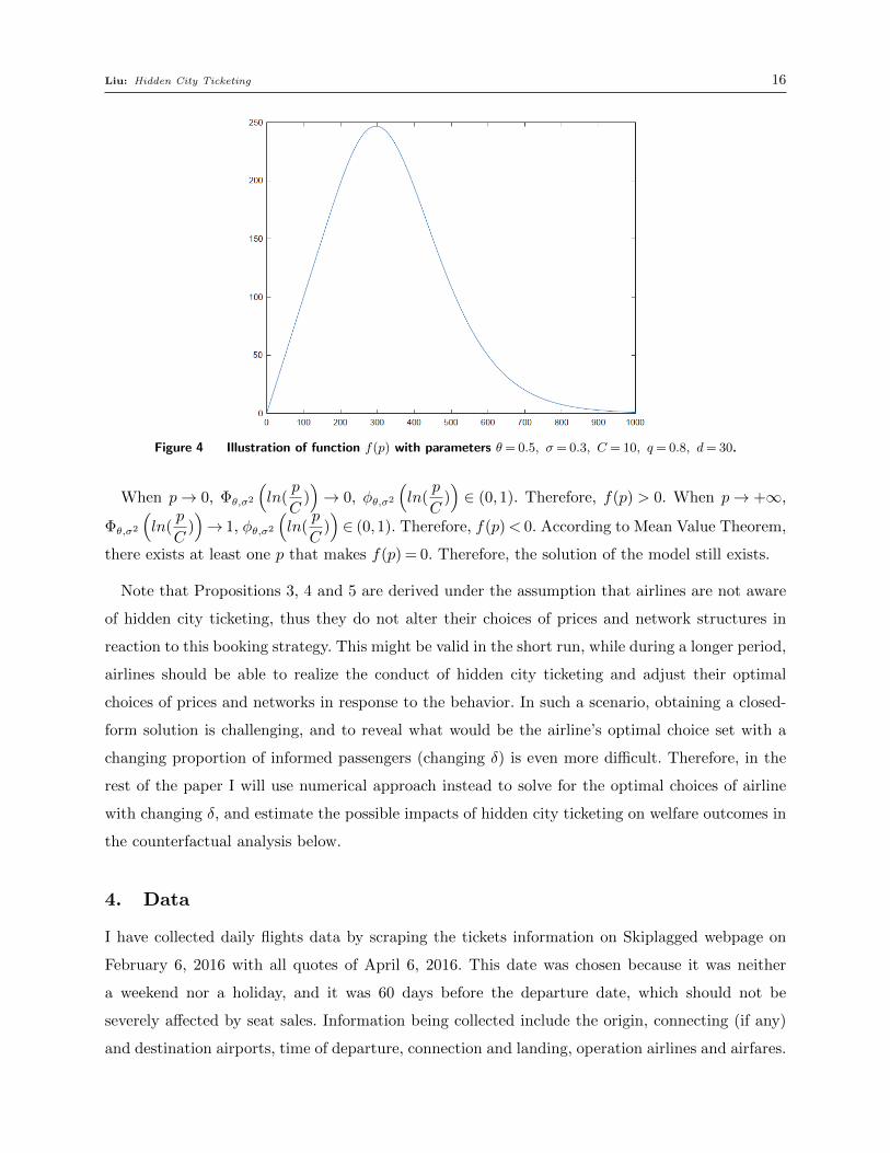
Therefore, the optimal price bundle is solvable. To further confirm that function f(p) = p ·[1−Φθ,σ2

(ln

(p

C · q · d

))]is unimodal, I depict function f(p) with parameters θ = 0.5, σ =

0.3, C = 10, q= 0.8, d= 30, as shown in Figure 4 below.

When there is hidden city ticketing, the difference lies in the optimal value of pABC . Instead of

looking for a pABC that maximizes pABC ·[1−ΦθABC ,σ

21

(ln

(pABC

C1 · qldABC

))], we are now solving

the following problem instead:

maxp

p ·[1−Φθ1,σ2

(ln(

p

C1

)

)]+ δ · p ·

[1−Φθ2,σ2

(ln(

p

C2

)

)]where C1 and C2 are constants.

Take derivative of the objective function and make it equal 0:

1−Φθ1,σ2

(ln(

p

C1

)

)−φθ1,σ2

(ln(

p

C1

)

)+ δ

[1−Φθ2,σ2

(ln(

p

C2

)

)−φθ2,σ2

(ln(

p

C2

)

)]= 0.

Left-hand side is a function of p, f(p) with p ∈ [0,+∞). It is continuous because it is a lin-

ear combination of probability density function and cumulative distribution function of normal

distribution, which are all continuous functions.


Figure 4 Illustration of function f(p) with parameters θ= 0.5, σ= 0.3, C = 10, q= 0.8, d= 30.

When p→ 0, Φθ,σ2

(ln(

p

C))→ 0, φθ,σ2

(ln(

p

C))∈ (0,1). Therefore, f(p) > 0. When p→ +∞,

Φθ,σ2

(ln(

p

C))→ 1, φθ,σ2

(ln(

p

C))∈ (0,1). Therefore, f(p)< 0. According to Mean Value Theorem,

there exists at least one p that makes f(p) = 0. Therefore, the solution of the model still exists.

Note that Propositions 3, 4 and 5 are derived under the assumption that airlines are not aware

of hidden city ticketing, thus they do not alter their choices of prices and network structures in

reaction to this booking strategy. This might be valid in the short run, while during a longer period,

airlines should be able to realize the conduct of hidden city ticketing and adjust their optimal

choices of prices and networks in response to the behavior. In such a scenario, obtaining a closed-

form solution is challenging, and to reveal what would be the airline’s optimal choice set with a

changing proportion of informed passengers (changing δ) is even more difficult. Therefore, in the

rest of the paper I will use numerical approach instead to solve for the optimal choices of airline

with changing δ, and estimate the possible impacts of hidden city ticketing on welfare outcomes in

the counterfactual analysis below.

4. Data

I have collected daily flights data by scraping the tickets information on Skiplagged webpage on

February 6, 2016 with all quotes of April 6, 2016. This date was chosen because it was neither

a weekend nor a holiday, and it was 60 days before the departure date, which should not be

severely affected by seat sales. Information being collected include the origin, connecting (if any)

and destination airports, time of departure, connection and landing, operation airlines and airfares.


Figure 5 Distribution of busy commercial service airports around United States.

According to the Passenger Boardings at Commercial Service Airports of Year 2014 released in

September 2015 by Federal Aviation Administration (FAA), there are more than 500 commercial

service airports around United States. To reduce the computational burden of collecting data, I

have restricted my sample to the 133 busy commercial service airports identified by FAA. Only

focusing on those 133 airports is reasonable because those airports actually accounted for 96.34%

of total passenger enplanements in 2014. The distribution of the busy commercial service airports

around United States is shown in Figure 5. From the graph we can see that my data has covered

airports in Alaska, Hawaii and Puerto Rico, while no airport in Wyoming has been identified as

busy commercial service airport in my analysis.

Overall, my sample includes 16,142 routes (airport A to airport B) and 2,822,086 itineraries

(flight from A to B with specific information of time, connection node, operation airline(s) and

airfare(s)). Flights are operated by 45 different airline companies, among which 11 companies show

some hidden city opportunities lying in the itineraries they operate.

To the best of my knowledge, there is no official definition of hidden city opportunity in existing

literatures. GAO (2001) define that “a hidden-city ticketing opportunity exists for business travelers

if the difference in airfares between the hub market and the spoke airport was $100 or more, and for


leisure passengers if the difference in airfares was $50 or more”. In this paper, I have constructed

two intuitive definitions of hidden city opportunity myself and listed below.

Definition 1 Hidden city opportunity exists if the cheapest non-stop ticket of that itinerary is still

more expensive than some indirect flight ticket with the direct destination as a connection node.

Definition 2 Hidden city opportunity exists if the non-stop ticket is more expensive than some

indirect flight ticket which shares exactly the same first segment of that itinerary.

The example being illustrated at the beginning of this paper belongs to the second scenario.

And the second definition is also the one being defined in Wang & Ye (2016).

According to the daily flights data I have collected, these two definitions show similar magnitude

with respect to hidden city opportunities. For example, among all the itineraries, the first definition

indicates a total of 366,754 (13.00%) flights and 1,095 (6.78%) routes that exhibit possible hidden

city opportunities. Those amounts of Definition 2 are 394,544 (13.98%) flights and 1,316 (8.15%)

routes respectively. This magnitude is slightly smaller compared to the findings in GAO (2001),

in which the authors find that among the selected markets for six major U.S. passenger airlines

in their data, 17% provided such opportunities. Table 1 shows the top 10 origin-destination pairs

with most hidden city opportunities, which are the same under both definitions.

Table 1 Top 10 Origin-Destination pairs with most hidden city itineraries

Popularity Origin Destination # of Itineraries % under Def.1 % under Def.2

1 ISP PHL 11105 3.03% 2.81%

2 SRQ CLT 8590 2.34% 2.18%

3 CAK CLT 5948 1.62% 1.51%

4 GRR ORD 5733 1.56% 1.45%

5 MSN ORD 5640 1.54% 1.43%

6 XNA ORD 5529 1.51% 1.40%

7 COS DEN 4000 1.09% 1.01%

8 FSD ORD 3665 1.00% 0.93%

9 CAE CLT 3659 1.00% 0.93%

10 ORF CLT 3540 0.97% 0.90%

Furthermore, the maximum payment reduction would be as large as 89.57% if hidden city tick-

eting is allowed. Table 2 shows the top 10 origin-destination pairs with the largest price differences,

which are slightly different under both definitions. These statistics help reveal the fact that hidden

city ticketing might no longer be negligible nowadays and related research becomes necessary and

valuable.


Table 2 Top 10 Origin-Destination pairs with largest price differences

Definition 1 Definition 2

Origin Destination % Saving Origin Destination % Saving

LGA IAH 89.57% LGA IAH 89.57%

CLE IAH 88.49% CLE IAH 88.49%

PHL DTW 87.54% PHL DTW 87.54%

IAH EWR 86.61% MKE MSP 86.65%

IAH IAD 86.36% IAH EWR 86.61%

DTW PHL 86.20% IAH IAD 86.36%

KOA SFO 85.87% DTW PHL 86.20%

SNA SLC 85.46% KOA SFO 85.87%

ICT MSP 85.38% SNA SLC 85.46%

CLE EWR 85.03% ICT MSP 85.38%

Recall that my primary data contains flights operated by 45 different airline companies, among

which 11 companies shown some hidden city opportunities lying in the itineraries they operated.

Table 3 exhibits the amounts of hidden city itineraries of these airlines unber both definitions.

We can see that the three largest airlines: American Airlines, Delta Air Lines and United Airlines

operated more than 99% of those itineraries. This is similar to the findings of Surry (2005), in

which he found that 96% of those hidden city discounts came from American Airlines, Delta Air

Lines, United Airlines and Alaska Airlines. All of them are major hub-and-spoke carriers and apply

a hub-and-spoke network business model.

Table 3 Number of hidden city itineraries of different airlines

Airline IATA Code Def.1: # of Itineraries (%) Def.2: # of Itineraries (%)

American Airlines AA 203096 (55.38%) 210287 (53.30%)

Delta Air Lines DL 93062 (25.38%) 106867 (27.09%)

United Airlines UA 69587 (18.98%) 76175 (19.31%)

Alaska Airlines AS 598 (0.16%) 666 (0.17%)

Hawaiian Airlines HA 221 (0.06%) 221 (0.06%)

Frontier Airlines F9 56 (0.02%) 157 (0.04%)

JetBlue Airways B6 48 (0.01%) 106 (0.03%)

Virgin America VX 29 (0.01%) 36 (0.01%)

Silver Airways 3M 11 (0.00%) 11 (0.00%)

Spirit Airlines NK 8 (0.00%) 11 (0.00%)

Sun Country Airlines SY 7 (0.00%) 7 (0.00%)

A notable exception is Southwest Airlines, where no hidden city opportunity is found in the

itineraries operated by it, and whose fare rules actually do not specifically prohibit the practice of

hidden city ticketing. Since Southwest Airlines is a typical operator of fully-connected network, this


finding in the real data is in accordance with my previous proposition that hidden city opportunity

does not exist under fully-connected network structure.

5. Estimation

To estimate the parameters of my model, firstly I retrieve all the ordered triplets (A-B-C) from

my primary dataset. Then, with all the observed information of prices, distances and consumers’

preferences, I choose the parameters of my model to maximize the likelihood of observed airlines’

choices of network structures. In order to deal with this implicit maximum likelihood function, I

have applied global optimization algorithms, more specifically, Pattern Search to solve the MLE

and estimate the parameters.

5.1. Sample Build-up

To build my own sample, the first step is to retrieve ordered triplets (A-B-C) from the 133 busy

commercial service airports of my primary dataset. The triplet needs to satisfy the following three

conditions: 1) it must include direct flight from A to B; 2) it must include direct flight from B to

C; 3) it must include either direct or one-stop indirect flight from A to C using B as the connection

node.

In total, I have obtained 114,635 ordered triplets from my dataset that satisfy the conditions

listed above. Based on the differences in condition 3), I divide them into three different types.

Type I includes only direct flight from A to C with a subsample size of 26,198. To estimate pABC

of Type I, I add observed pAB and pBC up manually. Type II includes only indirect flight from A

to C through B with a subsample size of 61,092. To estimate pAC of Type II, I use the observed

pAB and assume flights from A to B and A to C share the same price per mile: pAC =pABdAB· dAC .

Type III includes both direct flight from A to C and indirect flight from A to C through B, with

a subsample size of 27,345. d represents geodesic distance computed based on the longitude and

latitude of the pair-airports provided by Google Maps.

On each route j, assume that θj ∼N(µj, σ22). Recall that each individual i has a time preference

parameter of λi and on each route j, the distribution of consumers’ time preferences satisfies

λij ∼N(θj, σ21). Therefore, µj measures the dependency of the destination city on business travelers.

Previous literature have constructed several indexes to capture this characteristic. For example,

Borenstein (1989) and Borenstein & Rose (1994) built a tourism index at the MSA level based

on the ratio of hotel income to total personal income. Brueckner et al. (1992) and Stavins (2001)

assumed that the difference in January temperature between origin and destination cities could


Figure 6 Business travel index for each airport as the destination city.

serve as a proxy for tourism. Gerardi & Shapiro (2009) segmented their data into “leisure routes”

and “big-city routes” based on the ratio of accommodation earnings to total nonfarm earnings.

In this paper, I have constructed my own index based on Borenstein (2010) and data provided

by TripAdvisor. Borenstein (2010) provides an index of the share of commercial airline travel to

and from cities that is for business purposes, which is based on the 1995 American Travel Survey.

This index was also used as one of the measures in Puller & Taylor (2012) to distinguish between

“leisure” and “mixed” routes. The shortage for this index is that it only includes data for each

state and metropolitan statistical area, while city level data might be a better fit corresponding

to the location of an airport. To solve this problem, I have also collected data from TripAdvisor

(the largest travel site in the world) for each city, and compute the average number of the reviews

of hotels/lodging, vocation rentals, things to do, restaurants, and posts of forum, standardized

by the city population from 2010 census. The underlying assumption is that a larger number of

reviews on TripAdvisor might be an indicator of being more popular among leisure travelers, and

this city-level data together with the indices constructed by Borenstein (2010) should be able to

provide more complete information of the city’s characteristics. After taking exponential of the

opposite of the average number from TripAdvisor’s review data, I compute the mean of that and

the indices from Borenstein (2010) (both state-level and MSA-level) and get µ.

From Figure 6 we can see that the largest µ= 0.7450 belongs to Dallas Fort Worth International

Airport (DFW) in Texas, while Ellison Onizuka Kona International Airport (KOA) on the Island


of Hawaii has the smallest µ = 0.0773. In general, places that are more popular among tourists,

such as Orlando, Puerto Rico and Hawaii, get the smaller µ(s). While places such as Dallas, Austin

and Chicago that are more attractive to business travelers have larger µ(s).

5.2. Maximum Likelihood Estimation

Overall, I have a set of 7 parameters: ζ = (δ,C1,C2, σ1, σ2, qh, ql), with δ ∈ [0,1] as my

parameter of interest, and the others are nuisance parameters. Observed attributes in my

dataset include the prices, distances, and time preference indices on each route: xi =

(pAB,BC,AC,ABC , dAB,BC,AC,ABC , µAB,BC,AC,ABC). And observed decision variable is the airline’s net-

work choices: yi ∈ {FC,HS}.

The maximum likelihood estimation needs to be processed in 2 steps. Firstly, I sample

θAB,BC,AC,ABC from the normal distribution N|xi,σ2 . Then airline makes a decision to maximize

expected profits:

yi = arg maxy∈{FC,HS}

Π(xi, y, ζ).

The maximum likelihood estimation problem is therefore:

ζ̂ = arg maxζ

1

n

n∑i=1

log p(yi|xi; ζ),

with the probabilistic model as

Pr[yi = y|xi, ζ] = Prθ∼N |xi,σ2

[Π(xi, y, ζ, θ)≥Π(xi,¬y, ζ, θ)] .

5.3. Pattern Search

This maximum likelihood estimation is challenging because the likelihood is implicit with a random

sampling in the first step, and the gradient is also difficult to evaluate with respect to ζ. Here I

apply global optimization algorithms to solve this MLE problem. That is, for each ζt, obtain an

estimation of likelihood function:

log p(yi|xi; ζt) = log Prθ∼N|xi,σ2

[Π(xi, yi, ζt, θ)≥Π(xi,¬yi, ζt, θ)]

≈ log

{1

M

M∑m=1

1 [Π(xi, yi, ζt, θm)≥Π(xi,¬yi, ζt, θm)]

}.

I have tried several global optimization techniques including Pattern Search, Genetic Algorithm,

Simulated Annealing, etc., to get the optimal set of parameters ζ = (δ,C1,C2, σ1, σ2, qh, ql) that


maximizes my log likelihood function. It turns out that Pattern Search works best in this case. It

costs the shortest time; It achieves the maximum log likelihood; And it obtains quite similar and

robust results when I change the starting point from δ= 0.1,0.5 to 0.9.

Pattern Search algorithm fits this problem quite well because firstly, it does not require the

calculation of gradients of the objective function, which are quite difficult to compute in this case.

Secondly, it lends itself to constraints and boundaries. For example, it could deal with the constraint

that 0< ql < qh < 1 quite well in this case.

How does the Pattern Search algorithm operate? Pattern search applies polling method (Math-

Works (2018)) to find out the minimum of the objective function. Starting from an initial point,

it firstly generates a pattern of points, typically plus and minus the coordinate directions, times

a mesh size, and center this pattern on the current point. Then, for each point in this pattern,

evaluate the objective function and compare to the evaluation of the current point. If the minimum

objective in the pattern is smaller than the value at the current point, the poll is successful, and

the minimum point found becomes the current point. The mesh size is then doubled in order to

escape from a local minimum. If the poll is not successful, the current point is retained, and the

mesh size is then halved until it falls below a threshold when the iterations stop. Multiple starting

points could be used to insure that a robust minimum point has been reached regardless of the

choice of the initial point.

This algorithm is simple but powerful, provides a robust and straightforward method for global

optimization. It works well for the maximum likelihood function in this paper, which is derivative-

free with constraints and boundaries.

5.4. Estimation Results

The estimation results from Pattern Search are shown in Table 4 below.

Table 4 Results of MLE

log likelihood -0.3023

δ 0.0373

C1 10.0935

C2 0.3125

σ1 0.2094

σ2 0.7406

qh 0.7010

ql 0.1125


According to the estimation results, the informed passengers account for around 3.73% of the

whole population. This proportion appeals to be trivial at first glance, but it is not surprising

because those are the travelers who are not only informed of hidden city ticketing, but also exploit-

ing those opportunities, and whose behavior in fact result in affecting the choices made by airlines.

And in the counterfactual analysis section below, I will further show that even a small fraction of

informed passengers will affect airline’s choices of network structures and prices significantly.

In order to derive the confidence interval of my parameter of interest δ, again I apply numerical

approach using bootstrap to find out the standard errors. I run the MLE for 1,000 times, and for

each run, sample the entire data with replacement and construct a data set of equal size. The

sample mean of the 1,000 estimates of the MLE is 0.0296, and the standard error is the sample

standard deviation as 0.0093. We can see that δ is significantly different from zero at 99% confidence

interval.

In Figure 7, I have plotted the log likelihood as a function of δ with all other parameters being

constant at their optimal values. From the figure it is clear that δ= 3.73% is the global maximizer.

Recall that in my theoretical model, I have assumed that there is only one airline serving the three

cities, thus the firm charges monopoly airfares. Liu (2015) also made similar monopoly assumption

in the paper, and corresponding to this assumption, the author refined the data and only paid

attention to the routes with a single carrier operating one or two flights per day. Following this idea,

I also define route AB, BC, AC, or ABC as monopoly if there is only one single carrier providing

services on that route. Refining my sample of ordered triplets according to this condition results in

a subsample size of 36,645, comparing to the total sample size of 114,635 before. Applying the same

estimation algorithm, I have solved the MLE problem again based on the monopoly subsample,

and get an estimation of δ being equal to 0.0303. The result is not significantly different from the

0.0373 we obtain above from the whole sample.

Furthermore, on September 17, 2019, I collected daily flights data again by scraping the tickets

information on Skiplagged webpage with all quotes of October 1, 2019, which was neither a weekend

nor a holiday, and was two weeks (rather than two months) before the departure date. This different

dataset provides a slightly larger estimation of δ being equal to 0.0407, which is still not significantly

different from our previous result. These two analysis provide robustness of my empirical data and

my estimation methodology.

6. Counterfactual Analysis

Based on our previous analysis, given a longer horizon, airlines should be able to adjust their

prices and networks in response to hidden city ticketing, in order to maximize their expected


Figure 7 Up: Plot of log likelihood when δ varies from 0 to 1. Below: Plot of log likelihood when δ varies from

0 to 0.1 (zoom in).

profits. To reveal what would be the airline’s optimal joint choices of prices and network structures

when δ changes, and further estimate the possible impacts of hidden city ticketing on welfare

outcomes, I have conducted several counterfactual analysis using numerical approach below. Will

airline companies always suffer from revenue loss with hidden city ticketing? Will hidden city

ticketing always benifit consumers and social welfare? Should government enact regulations to

clearly prohibit or permit this booking ploy? My counterfactual experiments will help shed some

light on those important policy implications.

Basically, assume that the proportion of informed passengers (δ) increases from 0 to 100%, and

airline companies always choose optimal prices under different network structures to maximize


their expected profits when δ changes. After obtaining the optimal price bundle p∗ under different

networks, I compute the surplus of producer, consumer, and society according to our previous

analysis in Section 3. Then I plot producer surplus (blue), consumer surplus (red) and total sur-

plus (black) under fully-connected network (dotted line) and hub-and-spoke network (solid line)

respectively, when δ varies.

6.1. Fully-Connected Network Outperforms Hub-and-Spoke Network

Findings 1 Among all the 114,635 data points (i.e., ordered triplets A-B-C), 75,995 (66.29%) have

expected profits under fully-connected network being always higher than that under hub-and-spoke

network, regardless of the value of δ.

My first finding is that under major cases, fully-connected network creates higher expected

profits for airlines comparing to hub-and-spoke network, regardless of the proportion of informed

passengers. One example would be the ordered triplets MIA→SEA→COS (Miami International

Airport to Seattle-Tacoma International Airport to Colorado Springs Airport). Figure 8 shows the

surplus of producer, consumer, and society with different δ(s). The dotted lines are always horizonal

because according to my model, hidden city ticketing will not affect the welfare outcomes under

fully-connected network structure. It is clear that in this example, the dotted blue line is always

above the solid blue one, regardless of the value of δ, which means that for airlines operating from

Miami International Airport to Colorado Springs Airport, a direct flight always outperforms an

indirect one through Seattle-Tacoma International Airport. This is not surprising because flying

from Miami to Colorado through Seattle is counter intuitive.

When we plot the surplus in Figure 8, there is a pattern of kink, which is not uncommon and also

found in other examples. Digging deep I find what happens at the kink is that airlines keep raising

the price pABC in response to the increasing proportion of informed passengers, δ. Consumers

benefit at first because more and more informed travelers are able to exploit the hidden city

opportunities, pay lower prices and obtain extra utility. However, when the kink point is reached,

pABC hits the magnitude of pAB and hidden city opportunities disappear. The informed passengers

can no longer obtain extra utility, while since the new pABC turns out to be higher than the original

price without hidden city ticketing, those passengers flying from A to C through B also get hurt.

This is similar to what is called “detrimental externalities” in Varian (1980), in which the author

also found that sometimes more informed consumers would cause the price paid by uninformed

consumers to increase. This finding also helps confirm the concern mentioned in GAO (2001) that

allowing hidden city ticketing might lead to unintended consequences, including higher prices.


10 20 30 40 50 60 70 80 90 100

proportion of informed passengers (%)

200

300

400

500

600

700

800

900

1000

1100

surp

lus

Producer surplus, FC

Producer surplus, HS

Consumer surplus, FC

Consumer surplus, HS

Total surplus, FC

Total surplus, HS

Figure 8 Surplus for MIA→SEA→COS when δ changes.

6.2. Hub-and-Spoke Network Outperforms Fully-Connected Network

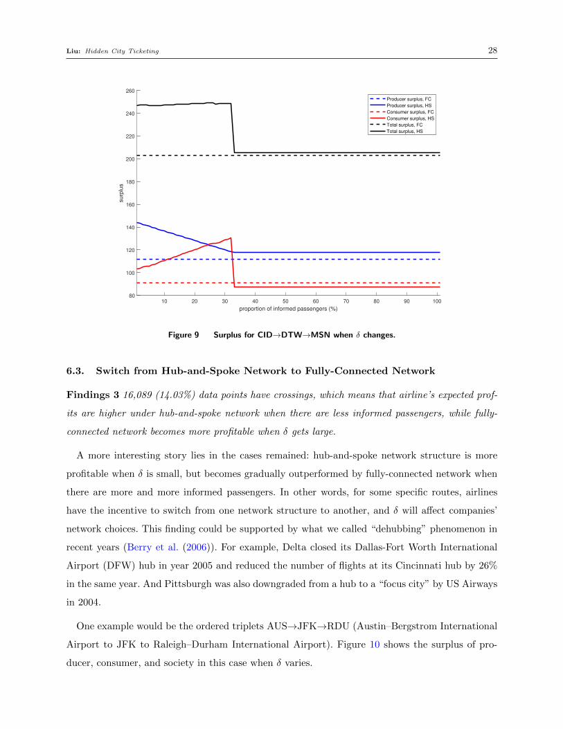
Findings 2 22,551 (19.67%) data points have expected profits under hub-and-spoke network being

always higher than that under fully-connected network, regardless of the value of δ.

Contradict to the previous finding, sometimes the hub-and-spoke network structure always does

a better job achieving higher revenue compared to fully-connected network. One example would

be the ordered triplets CID→DTW→MSN (The Eastern Iowa Airport to Detroit Metropolitan

Airport to Dane County Regional Airport in Madison). Figure 9 shows the surplus of producer,

consumer, and society in this case when δ varies.

We can see that the solid blue line is always above the dotted blue one, regardless of the value

of δ, which means that for airlines flying from The Eastern Iowa Airport to Dane County Regional

Airport in Madison, an indirect flight through Detroit Metropolitan Airport always outperforms a

direct flight. This usually happens when both airports A and C are small, which is exactly what

occurs when you are flying from CID to MSN. In this case, it might be costly for airlines to provide

a direct flight service, especially when compared to the relatively low demand.


10 20 30 40 50 60 70 80 90 100


80

100

120

140

160

180

200

220

240

260

surp

lus





Total surplus, FC

Total surplus, HS

Figure 9 Surplus for CID→DTW→MSN when δ changes.

6.3. Switch from Hub-and-Spoke Network to Fully-Connected Network

Findings 3 16,089 (14.03%) data points have crossings, which means that airline’s expected prof-

its are higher under hub-and-spoke network when there are less informed passengers, while fully-

connected network becomes more profitable when δ gets large.

A more interesting story lies in the cases remained: hub-and-spoke network structure is more

profitable when δ is small, but becomes gradually outperformed by fully-connected network when

there are more and more informed passengers. In other words, for some specific routes, airlines

have the incentive to switch from one network structure to another, and δ will affect companies’

network choices. This finding could be supported by what we called “dehubbing” phenomenon in

recent years (Berry et al. (2006)). For example, Delta closed its Dallas-Fort Worth International

Airport (DFW) hub in year 2005 and reduced the number of flights at its Cincinnati hub by 26%

in the same year. And Pittsburgh was also downgraded from a hub to a “focus city” by US Airways

in 2004.

One example would be the ordered triplets AUS→JFK→RDU (Austin–Bergstrom International

Airport to JFK to Raleigh–Durham International Airport). Figure 10 shows the surplus of pro-

ducer, consumer, and society in this case when δ varies.


10 20 30 40 50 60 70 80 90 100


150

200

250

300

350

400

450

500

550

600

650

surp

lus





Total surplus, FC

Total surplus, HS

Figure 10 Surplus for AUS→JFK→RDU when δ changes.

We can see that the solid blue line crosses the dotted blue one at the point when δ is around

6%, which means that when δ is smaller than the threshhold, airline would pursue hub-and-spoke

network structure. While when there are more and more informed passengers and δ crosses the

threshhold, airline has the incentive to switch from the hub-and-spoke network to fully-connected

network, and this decision will also affect both consumer surplus and total surplus dramatically.

In this example, after the airline company making the change, both consumer surplus and total

surplus increase a lot, which refer to the increase from the solid red, black lines to the dotted red,

black lines respectively. But this is not always the case, and we will see more details later in this

paper.

The crossing point varies for different ordered triplets. This is because different routes have differ-

ent characteristics and attract different types of travelers. Some routes would be quite “sensitive”

to hidden city ticketing and airlines operating on those routes would switch from hub-and-spoke

network to fully-connected network when δ is relatively small. Some routes would have operat-

ing airlines changing their network choices only when the amount of informed passengers are

large enough. And we have already known that sometimes airlines will never change to the fully-

connected network (Findings 2), while in other cases they will stick to the fully-connected network

from the very beginning (Findings 1). To have a more complete idea about the impact of different

δ(s) on airlines’ network choices, I can always depict the graph of surplus for every ordered triplet


Figure 11 Distribution of crossings when δ changes (pmf)

in my data. However, it is impossible to display all those figures here (recall that I have as many

as 114,635 data points in total). Therefore, in Figure 11 I have plotted the distribution of all the

crossing points when δ changes.

We can see that even a small δ matters. Airlines’ choices can be affected significantly even with

a quite small proportion of informed passengers. For example, airlines would switch from hub-

and-spoke network to fully-connected network on nearly 1,000 routes with only 1% of informed

passengers, and further change their choices on another 900 routes if the proportion increases to

2%. Recall that we have obtained an estimation of δ = 3.73% in Section 5, which appeals to be

trivial at first glance, but in fact, 3% of informed passengers could affect airlines’ choices of network

structures on approximately 2,700 routes (out of 16,089 in my whole sample), and this amount of

routes being affected would increase to around 3,600 when the proportion of informed passengers

increase to 4%. To make this illustration clearer, I have also drawn the cumulative distribution

function of the crossing points when δ varies from 0 to 1, and obtain my next finding from the

following Figure 12.

Findings 4 Airlines have the incentive to switch from hub-and-spoke network to fully-connected

network for half of the routes when there are approximately 10% of informed passengers, and for

75% of the routes when δ is only around 19%.

Recall that after airlines changing their choices of network structures, consumers and the whole

society are not always better off. After comparing the consumer surplus and total surplus before

and after the change for all those 16,089 routes, I am able to further conclude that:


Figure 12 Distribution of crossings when δ changes (cdf)

Findings 5 If airlines switch from hub-and-spoke network to fully-connected network, under

11,458 cases (71.22%) consumer surplus is going to increase, and under 11,128 (69.17%) cases

total surplus is going to increase.

In other words, unlike what could be derived from the theoretical model when airlines do not

alter their choices of network structures and airfares in the short run, during a longer horizon,

firms would actively react to the conduct of hidden city ticketing and change their optimal choices.

This will result in different welfare outcomes for producer, consumer, and whole society compared

to the propositions in Section 3. What I have found in my counterfactual analysis is that, during

this process, firms always result in lower expected profits, while consumers and the whole society

are not necessarily better off. Therefore, enacting a simple regulation for prohibiting or permitting

the conduct of hidden city ticketing would be difficult.

7. Discussion

There are some limitations and future questions remained in this paper. Firstly, I have made a

critical assumption in my model that there is only one airline serving the three cities, thus the

firm charges monopoly airfares. The monopoly assumption is not uncommon in airline related

literatures, but some researchers believe that after the deregulation, the US airline industry should

be characterized as being hightly oligopolistic (Shy (2001)). And in GAO (2001), the authors also

find that “hidden city opportunities may arise when a greater amount of competition exists for

travel between spoke communities than on routes to and from hub communities, and where airfares


in those markets reflect such competition”. In other words, besides the factors I have raised in my

propositions, competition might be another possible cause of hidden city ticketing, which does not

enter my model under the monopoly assumption. And given competition, besides the cost-saving

effect, another advantage of hub-and-spoke network compared to fully-connected network would

be that airlines could have stronger market power in the hub, which helps them increase the entry

barrier and drive up the prices for the origin-hub passengers. Since there are business travelers

who favor the origin-hub route and appeal to be price-inelastic, this market power of raising prices

could result in higher profits for the hubbing airlines. (Borenstein (1989), Borenstein (1991))

Another interesting question raised by Varian (1980) is that does it pay to be informed? If

this is true, a better way to take this into consideration might be assuming that it is possible to

become fully informed by paying a fixed cost C. Conducting hidden city tickeing is definitely costly.

Passengers are “threatened” by the airline companies and need to “bear some risk” to conduct this

behavior. As I have quoted from the contract of carriage in Section 1, consumers will be penalized if

being caught. And hidden city ticketing might be treated as “unethical” and a breach of the contract

between passengers and the airlines. There are also possible negative externalities such as causing

delays of the other passengers because of waiting and double checking baggages. Furthermore, the

condition of conducting hidden city ticketing is also highly restrictive. For example, if you have

luggage that is not carry-on, you are not able to leave the flight earlier without picking up your

bag. Normally, your checked baggage will be delivered to your final destination directly rather than

to your connection city. Also, you cannot conduct hidden city ticketing for the first segment of

your round-trip. Your second trip will be cancelled if you missed the connection of the first one.

Besides, you might need to bear the risk that you are switched to another flight because of initial

flight being cancelled or overbooked, with the same origin and destination airports, but bypass the

connection city. Therefore, cost will incur to be informed might be a reasonable assumption when

studying hidden city ticketing in the future, while measuring this cost would still be challenging.

Furthermore, airlines claim in the news that in reaction to the booking ploy of hidden city

ticketing, they might choose to charge more on flights, stop offering some flights, and re-calibrate

their no show algorithms. My analysis successfully predicts the increase in airfares of some flights.

But since I have assumed that airline companies are choosing between fully-connected network and

hub-and-spoke network, I do not provide an outside option for airlines to stop offering the flights

for certain routes. Instead of raising the prices of flights to eliminate hidden city ticketing, another

possibility is that the airlines could stop serving those defective routes. This is also another major

concern in GAO (2001) that allowing hidden city ticketing might result in unintended decreasing

service. Including this outside option could help make the analysis more complete, although the


Figure 13 Percentage of Passengers Denied Boarding by the U.S. Air Carriers, 1990 to 2019.

magnitude might be difficult to evaluate without a good measure of the costs. Another concern

raised by purchasing hidden city tickets is related to logistics and public-safety. When hidden

city ticketing becomes more popular, airlines might need to re-calibrate their no show algorithms.

They might have the incentive to oversell more, which is an act that could turn problematic

and expensive if the estimates are wrong. Unfortunately, I did not find the dataset of airlines’

oversales. Related statistics provided by United States Department of Transportation are numbers

of passengers boarded and denied boarding by the U.S. Air Carriers. Figure 13 shows the percentage

of passengers being denied boarding by the U.S. Air Carriers because of oversales, both voluntarily

and involuntarily, from year 1990 to 2019.

From Figure 13 we can see a declining trend of percentage of passengers being denied boarding

because of oversales in recent years, which indicates that the concern of possible oversales raised

by hidden city ticketing might be subtle.

8. Conclusion

To conclude, this paper aims at analyzing the possible cause and impact of hidden city ticketing. To

achieve this goal, I have constructed a structural model, collected innovative data, applied global

optimization algorithm to solve the MLE, and conducted counterfactual analysis. I find that hidden

city ticketing occurs only when airline companies are applying a hub-and-spoke network structure.


And airlines apply hub-and-spoke network rather than fully-connected network in order to reduce

their operation costs. When airlines are not aware of hidden city ticketing, hence do not alter their

choices of prices and network structures in the short run, we can derive from the theoretical model

that, 1) hidden city ticketing does not necessarily decrease airline’s expected profits, since the lower

price also attracts more passengers to take the flight; 2) consumers are always better off when

hidden city ticketing is allowed; 3) total social welfare always increase when hidden city ticketing

is allowed.

During a longer horizon, firms would actively react to the conduct of hidden city ticketing and

freely change their optimal choices of network structures and airfares. Under this circumstances,

based on the counterfactual analysis I have conducted, I find that 1) to maximize expected profits,

fully-connected network is always better than hub-and-spoke network for some routes (66.29%),

while hub-and-spoke network outperforms fully-connected network for some other routes (19.67%),

regardless of the proportion of informed passengers; 2) for the rest (14.03%) of the cases, airlines’

expected profits are larger under hub-and-spoke network when there are less informed passengers,

while fully-connected network becomes more profitable when more and more passengers starting

to exploit hidden city opportunities; 3) airlines have the incentive to switch from hub-and-spoke

network to fully-connected network for half of the routes when there are approximately 10% of

informed passengers, and for 75% of the routes when informed passengers increase to around 19%;

4) if airlines change their network choices because of hidden city ticketing, firms are suffering from

revenue loss, while consumers are not always better off (28.78% of the cases consumer surplus will

decrease), and total social welfare is not always larger neither (30.83% of the cases total surplus

will decrease). Therefore, enacting a simple regulation for prohibiting or permitting the conduct

of hidden city ticketing would be difficult, because welfare outcome varies route by route.

References

Berry, S., Carnall, M., & Spiller, P. T. (2006). Airline hubs: costs, markups and the implications of customer

heterogeneity. Competition policy and antitrust .

Berry, S., & Jia, P. (2010). Tracing the woes: An empirical analysis of the airline industry. American

Economic Journal: Microeconomics, 2 (3), 1–43.

Borenstein, S. (1989). Hubs and high fares: dominance and market power in the us airline industry. The

RAND Journal of Economics, (pp. 344–365).

Borenstein, S. (1991). The dominant-firm advantage in multiproduct industries: Evidence from the us airlines.

The Quarterly Journal of Economics, 106 (4), 1237–1266.


Borenstein, S. (2010). An index of inter-city business travel for use in domestic airline competition analysis.

NBER working paper .

Borenstein, S., & Rose, N. L. (1994). Competition and price dispersion in the us airline industry. Journal

of Political Economy , 102 (4), 653–683.

Brueckner, J. K., Dyer, N. J., & Spiller, P. T. (1992). Fare determination in airline hub-and-spoke networks.

The RAND Journal of Economics, (pp. 309–333).

Brueckner, J. K., & Spiller, P. T. (1994). Economies of traffic density in the deregulated airline industry.

The Journal of Law and Economics, 37 (2), 379–415.

Caves, D. W., Christensen, L. R., & Tretheway, M. W. (1984). Economies of density versus economies of

scale: why trunk and local service airline costs differ. The RAND Journal of Economics, (pp. 471–489).

Dana, J. D., Jr (1998). Advance-purchase discounts and price discrimination in competitive markets. Journal

of Political Economy , 106 (2), 395–422.

Escobari, D., & Jindapon, P. (2014). Price discrimination through refund contracts in airlines. International

Journal of Industrial Organization, 34 , 1–8.

GAO (2001). Aviation competition: Restricting airline ticketing rules unlikely to help consumers. Report to

Congressional Committees, U.S.Government Accountability Office, Washington, DC..

URL https://www.gao.gov/products/GAO-01-831

Gerardi, K. S., & Shapiro, A. H. (2009). Does competition reduce price dispersion? new evidence from the

airline industry. Journal of Political Economy , 117 (1), 1–37.

Giaume, S., & Guillou, S. (2004). Price discrimination and concentration in european airline markets. Journal

of Air Transport Management , 10 (5), 305–310.

Lazarev, J. (2013). The welfare effects of intertemporal price discrimination: an empirical analysis of airline

pricing in us monopoly markets. New York University .

Liu, D. (2015). A model of optimal consumer search and price discrimination in the airline industry.

MathWorks (2018). Pattern search, accessed 3-october-2018.

URL https://www.mathworks.com/help/gads/patternsearch-climbs-mt-washington.html

Puller, S. L., & Taylor, L. M. (2012). Price discrimination by day-of-week of purchase: Evidence from the

us airline industry. Journal of Economic Behavior & Organization, 84 (3), 801–812.

Rao, V. R. (2009). Handbook of pricing research in marketing . Edward Elgar Publishing.

Robert S, P., & Daniel L, R. (2001). Microeconomics.

Shy, O. (2001). The economics of network industries. Cambridge university press.

Stavins, J. (2001). Price discrimination in the airline market: The effect of market concentration. Review of

Economics and Statistics, 83 (1), 200–202.

https://www.gao.gov/products/GAO-01-831

https://www.mathworks.com/help/gads/patternsearch-climbs-mt- washington.html


Surry, P. (2005). Hidden city ticket opportunities are more common than you think. Hopper Research..

URL https://media.hopper.com/research/hidden-city-ticket-opportunities-common-think

Varian, H. R. (1980). A model of sales. The American economic review , 70 (4), 651–659.

Wang, Z., & Ye, Y. (2016). Hidden-city ticketing: the cause and impact. Transportation Science, 50 (1),

288–305.

https://media.hopper.com/research/hidden-city-ticket-opportunities-common-think

paying more for a shorter flight? - hidden city ticketing

Documents