Pattern-Seeking Behavior

Senior ProjectSubmitted to the Division of Science, Math and Computing

Bard CollegeAnnandale-on-Hudson, NY

Max HowardMay, 2012

Multilayer Perceptron and Back Propagation withMomentum Applied to Stock Price Movements in 2006

Table of Contents

Chapter1. Introduction...........................................................................................1

1.1. Project Goal............................................................................11.2. Tulipomania........................................................................1-31.3. Market Irrationality.............................................................3-5

2. Background...........................................................................................62.1. Artificial Neural Networks.....................................................62.2. Perceptrons and Multilayer Perceptrons.............................6-72.3. Supervised Learning...........................................................7-82.4. Back-propagation with Momentum....................................8-92.5. Batch Learning vs Online Learning.......................................92.6. Economic Factors.................................................................102.7. Securities.........................................................................10-12

3. Project..................................................................................................133.1. Economic Metrics.................................................................133.2. Data Collection Process...................................................13-14

4. Results..................................................................................................154.1. Methodology.........................................................................154.2. Iris Test Set......................................................................15-164.3. Data Collection.....................................................................164.4. Data Pre-processing.........................................................16-184.5. Data Alteration.................................................................19-214.6. Learning Rate and Momentum........................................21-224.7. Maximum Error...............................................................22-234.8. Network Architectures.....................................................24-25

5. Conclusions.........................................................................................265.1. Standard of Success..............................................................265.2. Short Selling....................................................................26-275.3. Scaling..................................................................................275.4. Predictors.........................................................................27-285.5. Optimal Maximum Error......................................................28 5.6. Optimal Network Architectures...........................................285.7. Delta.....................................................................................295.8. Monetary Analysis................................................................295.9. Trading Patterns..............................................................29-31

Works Cited.............................................................................................32

List of Figures

Chapter1. Introduction

Figure 1.3.1. VIX Graph with Bubble Overlay.............................4

2. BackgroundFigure 2.3.1. MLP.........................................................................8

4. ResultsFigure 4.4.1. Architectures with GE Average Net Error..............17 Figure 4.4.2. 4-Day Predictor.......................................................17 Figure 4.4.3. 2-Day Predictor.......................................................18 Figure 4.4.4. 3-Day Predictor.......................................................18 Figure 4.6.1. Data Scaling Example.............................................19 Figure 4.6.2. Partially Scaled vs Fully Scaled AverageNetwork Error for All Sectors......................................................20 Figure 4.6.3. Delta vs Non-Delta Average Network Error for GE.................................................................................21 Figure 4.6.4. Delta Average Network Error for All Sectors........21 Figure 4.7.1. Maximum Error and Average Network Error for GE...........................................................................................23 Figure 4.7.2. Maximum Error and Average Network Error for All Sectors...............................................................................23 Figure 4.8.1. Architectures and Average Network Error for GE................................................................................................24 Figure 4.8.2.Architectures and Average Network Error forAll Sectors....................................................................................25

5. ConclusionsFigure 5.9.1 Trading Data for All Sectors Jun-December 2006.............................................................................................31

PREFACE

“12:45, restate my assumptions: 1. Mathematics is the language of nature. 2. Everything around us can be represented and understood through numbers. 3. If you graph these numbers, patterns emerge. Therefore: There are patterns everywhere in nature.” (Pi, 1998)

When Darren Aronofsky wrote and directed his first Hollywood film, Pi, it is doubtful

he intended the movie to be an allusion to the work of a Bard CS major, fourteen years in

the future. Yet there are uncanny similarities between the two, best illustrated by a quick

description of a scene from the movie.

The protagonist - Max, as it happens – slouches, alone in a room filled with computers,

gazing disinterestedly at a ticker board displaying an endless string of stock price

updates. “Six and a half,” he murmurs. A moment later 6 ½ tumbles across the

board. “Seven and a quarter”. This number soon materializes as well. “Thirteen”. We

know what happens next. Preceding this sequence, Max has spent the majority of his time

simultaneously slipping into psychosis and designing a computer algorithm that predicts

the next day’s stock prices – a project with which is, at last, complete.

Critics’ reviews of Aronofsky’s 1998 film describe the film’s reception. There is

commentary surrounding the film’s “disconcerting surrealism” and “uncomfortable

subject matter”; but by far the most common sentiment is that it straddles the line

between science and science fiction. Roger Ebert, writing in 2000, in the Chicago Sun-

Times - “The seductive thing about Aronofsky’s film is that it is halfway plausible in

terms of modern physics and math.” Only halfway plausible, Mr. Ebert? I beg to differ.

1

1. INTRODUCTION

1.1. Project Goal

The goal of this project is to investigate the possibility of training a neural network to predict

stock market price action, explore how several parameters affect its performance and to

distill a single model producing the most accurate price estimates. Many traditional models,

such as those used in “value investing”, employ market metrics with the purpose of

determining whether a security is over or under valued. Yet, while the notion of assigning

value seems intuitive, these models contain an inherent bias towards the theory that markets

act rationally. Neural networks, which use pattern matching, and make no such assumptions,

may be more predictive, because in fact, markets are prone to acting irrationally.

1.2. Tulipomania

In 1841, Scottish journalist Charles Mackay published his magnum opus: Extraordinary

Popular Delusions and the Madness of Crowds [1]. This two-volume work, chronicling

events ranging in category from “Philosophical Delusions” to “Popular Admiration of Great

Thieves”, is among the classic histories of social psychology and psychopathology. Of

particular relevance to this project, however, is Mackay’s account of what may be the most

fantastical of any subject found within the text - tulipomania.

Tulips were introduced to Europe in 1554 by Ogier de Busbecq, Austrian ambassador to the

Holy Roman Emperor in Constantinople, when he mailed the flowering bulbs to Vienna.

They quickly gained popularity, thanks in part to an infection known as the Tulip Breaking

2

Virus which “broke” the afflicted tulip’s lock on a single color, creating a range of much

more striking blooms, but also limiting the plant’s ability to propagate. No country took to

them with as much enthusiasm as the United Provinces (modern day Netherlands); and by

1610, Dutch traders had started commodifying this new product, from production to

consumption. They bartered contracts obligating a buyer to purchase Tulip bulbs at a

predetermined date, and options allowing the owner to buy and sell bulbs at a predetermined

price (futures, calls and puts respectively). With bulbs having limited supply, high demand

and no intrinsic value, there was only one choice afforded to the Dutch traders who didn’t

want to be left out: pay ever increasing prices for the same product. And thus began the first

speculative “bubble” in recorded history.

According to anti-speculative pamphlets written just after this bubble, in early November

1636, a Viceroij tulip bulb cost around five Dutch guilders ($360). By February 3, 1637, a

Viceroij tulip bulb was among the most expensive objects on the planet, with one recorded

sale reaching forty two hundred guilders, close to US $3,000,000 adjusted for inflation, or an

8,400% increase in price. Then, before the month was out, the market for bulbs evaporated.

Haarlem, a coastal city in the United Provinces, was at the height of an outbreak of the

bubonic plague when buyers, fearing for their wallets and lives, refused to show up at a

routine bulb auction. By May 1, Viceroij bulbs were worth 1/1000th of their value at the

beginning of February. It was as if the whole thing had never happened – the bubble had

burst [2].

3

Wagon of Fools, by 17th century Dutch painter Hendrik Gerritsz, depicts a group of Dutch

weavers who, emboldened by their newfound prosperity, have abandoned their trade to ride

around on a wagon, drink wine and count money. Their future can be surmised from the

wagon to their right, which is disappearing into the ocean [3].

1.3. Market Irrationality While Tulipomania was limited to Dutch tulip speculators, it is a shining example of a truth

that has presented itself again and again - markets often act irrationally. Even today, we are

witnessing a congruent event in the cloud computing giant Salesforce.com. [4] The company,

which has quintupled in price over the last three years, has a P/E ratio of over 8,000 and a

forward P/E ratio of 75 (meaning the stock is predicted to increase its earnings per share or

decrease its price by a multiple of at least 7,900 over the next 12 month period). Holding the

price constant, with a current earnings per share of $0.10, and 130M shares outstanding,

4

Salesforce would need to generate a profit of just over ten trillion dollars (0.10 x 7,900 x

130,000,000 = $10,273,600,000) over the next twelve months to accomplish this, or about

four times the gross tax receipts collected by the US Treasury Department in 2007. For a firm

with a market cap of less that $22 billion [5], even the world’s most creative accounting

firms would be hard pressed to bridge this gap.

Interestingly enough, it is during the course of bubbles that we have begun to see historic

lows in stock market volatility. The VIX, also known as “fear gauge”, is the most commonly

accepted volatility metric [6]. It is computed using the number of at-the-money puts and calls

written and bought. Essentially, the more investors speculate the market will move, towards

one extreme or another, the higher the VIX. Shown below is a graph displaying the VIX

during the time period.

Figure 1.1.1 VIX Graph with Bubble Overlay

5

In an attempt to avoid the problems introduced during high volatility, a factor that may

inhibit pattern detection, this project considers one of these “bubble” periods and employs

Artificial Neural Networks (ANNs) to analyze newly visible patterns in stock price action.

6

2. BACKGROUND

2.1. Artificial Neural Networks

To understand how an ANN functions, it is useful to first understand what it models, which

is, quite simply, the human brain. The brain of an adult human typically contains between 50

and 100 billion neurons. Each neuron is connected to other neurons via junctions called

synapses, which enable the transmission of neural impulses. There are thought to be between

100 and 500 trillion of these neural connections in the brain [5]. One neuron, taken by itself,

has a relatively small amount of computational power. But, taken along with tens of billions

of other neurons, and connected by the specific patterns of synapses residing in each human

brain, they allow human beings to attempt the widest range of tasks.

2.2. Perceptrons and Multilayer Perceptrons

There are many types of ANNs, each specializing in completing different objectives. In the

ANN employed for by this project, the multilayer perceptron (MLP), neurons and synapses

are represented by perceptrons and weighted connections. Weighted connections take a

rational number input, multiply it by the weight of the connection, and output the result. Each

input to a perceptron passes through a distinct weighted connection, then they are summed

up, and a bias (typically negative) is added to the total. If the total is greater than 0, then the

perceptron outputs 1, otherwise 0.

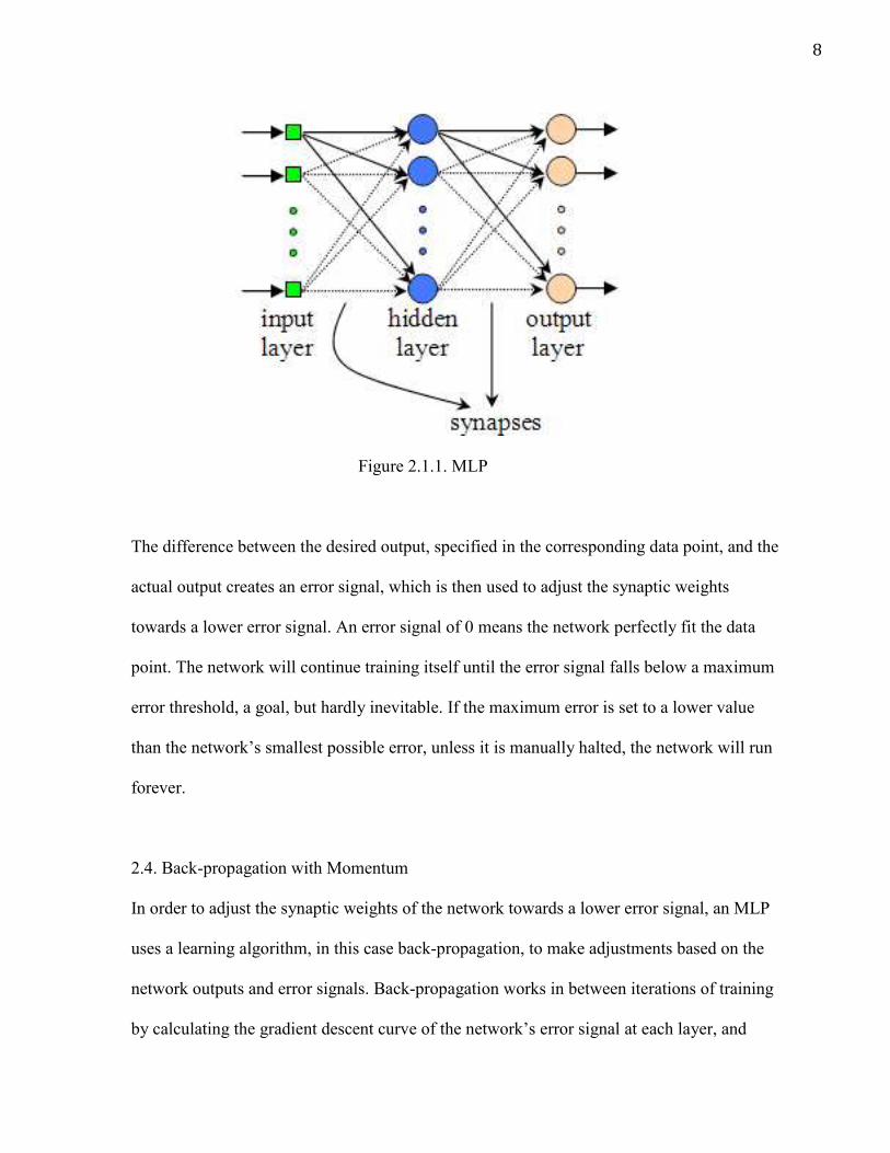
Multilayer perceptrons are arranged into at least three layers of perceptrons: an input layer (in

which the user specifies the inputs); some natural number of hidden layers (which is where a

7

majority of the relevant computational adjustments to the network [learning] take place); and

an output layer (where the network specifies which output the input data was mapped to).

The MLP uses modified perceptrons which, instead of outputting 0 or 1, directly output the

biased sum. In a fully connected MLP, such as the one used in this project, the output of each

perceptron is connected via a weighted connection to each perceptron in the following layer

[6]. Employment of an MLP occurs in two steps: training and testing.

2.3. Supervised Learning Multilayer perceptrons are trained using a supervised learning paradigm, in which a set of

data points, each composed of both inputs and desired outputs, are fed to the network. The

number of neurons (perceptrons) in the input layer will be the same as the number of inputs.

One round of training on a single data point passes each input value in the data point to a

single corresponding input neuron. Since the MLP is fully connected, the output value

calculated by each neuron in the input layer will be sent, via a weighted connection, to each

neuron in the second layer (one of the hidden layers). Each neuron in the second layer will

have exactly as many incoming connections as there are nodes in the input layer. The input

signal will continue to filter through the network in this fashion until it reaches the output

layer, which is composed of exactly as many neurons as there are outputs in the data point.

Finally, the network will generate an output: the set of values returned by each of the output

neurons.

8

Figure 2.1.1. MLP

The difference between the desired output, specified in the corresponding data point, and the

actual output creates an error signal, which is then used to adjust the synaptic weights

towards a lower error signal. An error signal of 0 means the network perfectly fit the data

point. The network will continue training itself until the error signal falls below a maximum

error threshold, a goal, but hardly inevitable. If the maximum error is set to a lower value

than the network’s smallest possible error, unless it is manually halted, the network will run

forever.

2.4. Back-propagation with Momentum

In order to adjust the synaptic weights of the network towards a lower error signal, an MLP

uses a learning algorithm, in this case back-propagation, to make adjustments based on the

network outputs and error signals. Back-propagation works in between iterations of training

by calculating the gradient descent curve of the network’s error signal at each layer, and

9

adjusting the network’s synaptic weights towards a lower error. In essence, it breaks down

the network’s error signals, determines which direction each weight would have to be

adjusted in order to minimize the error signal, then changes each weight according to two

values: learning rate and momentum.

Learning rate is a static parameter set by the user, which specifies exactly how much the net

changes each weight in one round of training. Momentum is also user defined and, is a

changing multiplier, calculated as a function of the previous weight change, and used in

conjunction with the learning rate to effect how much weights are changed each round.

Consecutive weight changes in the same direction will increase the momentum multiplier,

causing the synaptic weights to change by larger amounts. A weight change in the opposite

direction will decrease the momentum multiplier [7].

2.5. Batch Learning vs Online Learning

Adjustments to the synaptic weights of the net can take place at two times, depending on the

training method. Batch-learning applies the learning algorithm to the network after all of the

data points have been assessed, and uses the combined error signal. Online learning applies

the learning algorithm to the network immediately after each data point is assessed, using the

individual error signals. This study’s MLP employs the online learning training method as it

was the only option permitted by the software used.

10

2.6. Economic Factors The design of the MLP used in this project originally included nine economic factors, since

whittled down to three. These are:

1. Price of a given stock taken at the end of the trading day, but before

after hours trading commences.

2. Williams’ Percent Range Technical Indicator (W%R) is a 0-100

range bound technical indicator, which compares a stock’s close to its

range of highs and lows over the last 14 days [8]. It is most often used

as a measure of whether the stock is overbought or oversold. Readings

over 80 suggest the stock is underbought/oversold while readings

below 20 indicate that it is overbought/undersold.

3. Parabolic Stop and Reverse (PSAR) is a momentum indicator which

uses most recent price extremes and an acceleration factor to

determine future points on a parabolic arc [9]. It is most commonly

applied to signal a trader to consolidate his/her gains (ie. liquidate long

positions and close out short positions).

2.7. Securities In the present study, the network applied these parameters to four categories of securities in

the year 2006. To be selected, each of the four companies had to satisfy two constraints: price

11

range and maturity. Over the course of the entire year, each company was not allowed to

fluctuate in price by more than 50% from its starting price. Each company also had been

publicly traded for at least 20 years, and was trading at a price no more than 20 times its

earnings over the last 12 months (P/E ratio). These limitations were created in order to

exclude companies that had suffered catastrophic meltdowns or unprecedented windfalls,

neither of which are predictable.

1. Utilities

Consolidated Edison (ED), one of the largest investor owned utility

companies in the United States, headquartered in New York.

2. Technology

International Business Machines Corporation (IBM), an American

multinational technology hardware and consulting corporation

headquartered in New York. As of 2011, IBM was the second largest

publicly traded technology company in the world.

3. Industry

General Electric Corporation (GE), a multinational conglomerate

headquartered in Connecticut , which operates four segments: energy,

technology, capital finance, and consumer & industrial products.

12

4. Consumer Products

Johnson & Johnson (JNJ), a New Jersey-based multinational

manufacturers of pharmaceutical, diagnostic, therapeutic, surgical, and

biotechnology products.

13

3. PROJECT

3.1. Economic Metrics This project began with quite different goals than those pursued here. First, while the

intention of using periods of low VIX began at conception, this study was originally intended

to make use of much broader economic metrics, including the employment rate, and new

orders for durable goods, both of which were to be tested in tandem with a selection of peer

measurements until the optimal combination was found. Data for nine economic metrics was

collected before it became clear that, because these metrics were calculated monthly, and the

periods of low VIX lasted roughly 5 years each, only around 60 data points could be

collected, not nearly enough. Thus, this methodology and the corresponding goal of

employing a neural network to predict macro economic stock trends were replaced with

smaller-scale version of themselves: market metrics released daily instead of monthly and

price predictions on the scale of weather forecasts.

3.2. Data Collection Process Second, the original idea was to build a custom application that would allow for the control

of every aspect of the network. Fortunately such a software tool already existed: Neuroph

Studios, a fully featured Java neural network framework available for free on

sourceforce.net. This Java application offered control over network architecture, data format,

transfer methods (sigmoid vs tangential), learning algorithms, maximum error, learning rate,

momentum and connectivity. The application graphs network training in real time, tracking

the number of iterations and network error output, and even placed testing errors into a .txt

14

file cumulatively, which meant training and testing could be done continuously, to build one

large sheet of results [10]. Combined with a custom-built Java program that took .txt files,

discarded irrelevant characters, and averaged absolute values of the network errors from each

round of training and testing, processing results could be completed in an efficient and error

free manner.

Finally, with respect to data collection itself, while this project set out to collect and test data

from twelve different companies, it completed collection from four, one from each sector:

utilities, industry, technology and consumer products. The collection of data sets was done

completely by hand using Yahoo! Finance. The organization of data into test and training

sets was done using a combination of Microsoft Excel,www.random.org/lists and TextEdit.

Microsoft Excel was used to format the data into data points for the neural network,

www.random.org/lists randomized the lines of data points and TextEdit was used to separate

the data into training and test sets.

Training a network for the first time is a daunting task. Data format, learning rate, maximum

error and momentum all must be within a very small range of values for the network to

function correctly. This project was aided by data from previous Neuroph Studios users,

especially a 2010 report detailing the exact values and architecture used to successfully train

and test a net accepting the iris test set [11]. Building upon this success, the project was

launched and proceeded directly to collecting market data.

15

4. RESULTS

4.1. Methodology With the goal in mind of minimizing average network error (using the same data set but

getting better results), testing and subsequent adjustment phases of this project were broken

down into 5 segments:

1. Data collection 2. Data pre-processing 3. Tuning learning rate and momentum 4. Testing with different values of maximum error 5. Testing with different network architectures

During each segment, all other factors were held constant so as the give the clearest

indications of how to adjust that parameter. In order to present the data in a manageable and

concise format, unless otherwise stated, all results included were calculated using the data set

that produced the best results, the GE data set.

4.2. Iris Test Set

Before beginning to work with market data, tests were run working with a simpler data set. In

1936, an American botanist named Edgar Anderson assembled data quantifying the

morphological variations in three different species of Iris flowers [12]. Since then, his data

set has found numerous scientific applications, including serving as a classical test case for

classification techniques using machine learning. The base net for this project was conceived

using this test set as a starting point, and was considered immediately complete when it

achieved an accuracy of 99.99%. First, the Iris flower data set was composed of 150 separate

data points, so each data set used in this project has at least 150 points. Second, the net which

16

accepted the flower data had one hidden layer and one more hidden nodes than the number of

input nodes, and this relationship was reflected in the base net. Lastly, the maximum error,

learning rate and momentum that most rapidly trained the net and resulted in the lowest

average net error were carried over as well. Though the final neural network is vastly

different, it can be retraced to this initial base net designed to classify flowers. Guiding this

decision was an emphasis on the structure, rather than the content of this study.

4.3. Data Collection

Data collection consisted of gathering daily price, PSAR and W %R readings from Yahoo!

Finance between early June 2006 and January 2007, the period of lowest sustained volatility

in the last 20 years. Though ultimately unused, metrics released monthly from the U.S.

Department of Commerce were also collected.

4.4. Data Pre-processing

Data pre-processing took place in two steps: arrangement (which determined the content and

structure of the data), and alteration (which was used to test different training methods). Data

arrangement proceeded following the hypothesis of this project: patterns in past market

activity can be used to predict future price action. Training sets were designed to reflect this,

using price, PSAR and W %R from consecutive days and price alone from the last day. 2-

day, 3-day and 4-day predictors were used. For reference, a neural network with 3 inputs,

two hidden layers consisting of 7 nodes and 2 nodes, the layer with 7 coming first, and 4

outputs would be represented as 3-7-2-4. Results were recorded in elementary form, as

network error/data points in test set, using the three hidden layer configurations: 9-10-5-1, 9-

17

5-1 and 9-10-1. A max error of 0.0009 was used. Lowest average net error per data point

indicates which number of days is most predictive.

Architecture 4-day 3-day 2-day 9-10-5-1 0.0422 0.0393 0.0614 9-5-1 0.0472 0.0422 0.061 9-10-1 0.049 0.0434 0.0632

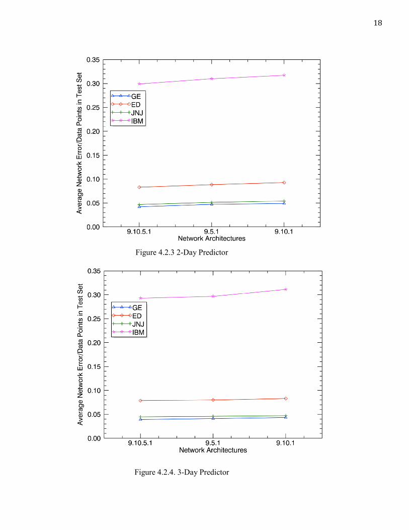
Figure 4.1.1 Architectures with GE Average Net Error Plotted below are the 4-day, 3-day and 2-day predictor results for all four sectors.

Figure 4.2.2. 4-Day Predictor

18

Figure 4.2.3 2-Day Predictor

Figure 4.2.4. 3-Day Predictor

19

4.5. Data Alteration

Data alteration was carried out in a number of ways, but can be expressed in two categories:

scaling and Delta. Scaling was used to solve one of the most basic issues with the collections

of raw data. Neural networks are generally optimized to train on data ranging from 0 to 1 or -

1 to 1, depending on the transfer function, and the nets used in this project were no exception.

Raw data came in the form of numbers ranging from -100 in the case of W %R to the highest

prices and PSAR readings, which were generally about the same, so data alteration was

necessitated for the net to accept the training set.

Since to W %R is range-bound between -100 and 0, scaling this number required simply

multiplying it by -0.01. Price is not range bound; so to make the parameter scale from 0 to 1,

first the minimum value was pin-pointed and subtracted from the entire column of prices,

then the new maximum was divided into 1, to find a multiplier. Finally, the multiplier was

applied to all prices, and PSAR altered in the same way.

EXAMPLE

Price New Price Final Price 75 50 1 50 Min Price: 25 25 Max Price: 50 0.5 25 0 Multiplier: 1/50 0

Figure 4.5.1. Data Scaling Example

Ten rounds of training and testing were completed on each set using a max error of 0.0009.

Results were recorded as average network error/number of data points in the test set. For

20

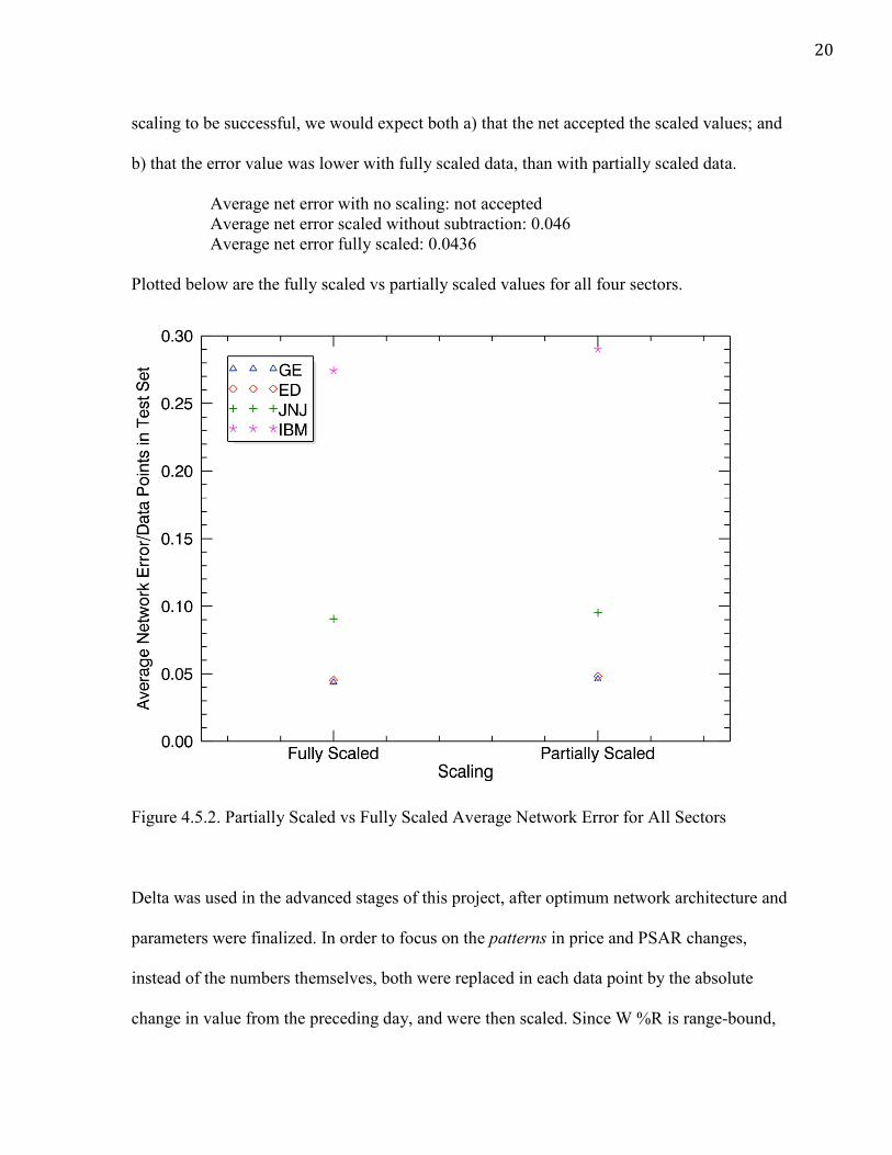
scaling to be successful, we would expect both a) that the net accepted the scaled values; and

b) that the error value was lower with fully scaled data, than with partially scaled data.

Average net error with no scaling: not accepted Average net error scaled without subtraction: 0.046 Average net error fully scaled: 0.0436

Plotted below are the fully scaled vs partially scaled values for all four sectors.

Figure 4.5.2. Partially Scaled vs Fully Scaled Average Network Error for All Sectors

Delta was used in the advanced stages of this project, after optimum network architecture and

parameters were finalized. In order to focus on the patterns in price and PSAR changes,

instead of the numbers themselves, both were replaced in each data point by the absolute

change in value from the preceding day, and were then scaled. Since W %R is range-bound,

21

it was not altered in this way. Delta and non-delta sets were tested on a number of different

nets, using an ME of 0.0009. Results were reported as average network error/data points in

the test set. For delta to be considered successful, the smallest delta value should be smaller

than the corresponding non-delta value, and the smallest delta value should be below .0377,

or the lowest average network error obtained from scaled non-delta data.

Architecture Delta Non-Delta 9:10:10:1 0.0319 0.0384 9:10:5:1 0.0313 0.0377 9:10:1 0.0331 0.0398 9:5:5:1 0.0325 0.0391

Figure 4.5.3. Delta vs Non-Delta Average Network Error for GE

Company 9:10:5:1 Error GE 0.0313 JNJ 0.0341 IBM 0.261 ED 0.0875

Figure 4.5.4. Delta Average Network Error for All Sectors 4.6. Learning Rate and Momentum Learning rate and momentum, being the means by which a network’s learning speed is

controlled, changed very little from the base net. Momentum was initially increased to reduce

training times, but this was an adjustment in proportion to a lower maximum error, which

was eventually dropped. In the end, learning rate stayed exactly the same at 0.6 and,

momentum was set at 0.3. Though it was very important to find workable values for learning

22

rate and momentum, after these were determined, there was no further testing or data

collection. These parameters remained the same as the base net.

4.7. Maximum Error

Maximum net error was adjusted to maintain the balance between maximizing pattern

detection and over-fitting. Recall that a neural network only halts “training” after its net error

output dips below the maximum error (ME) parameter. When the ME is too high, the

network will not have enough time to train, and pattern detection will suffer. When the ME is

too low, the network will be subject to over-fitting. In other words, the network learns the

patterns of the training set too well, and is not flexible enough to detect patterns in the test

set.

This project considered a range of maximum errors starting with the base net’s 0.01, with

which the net took 2 iterations to halt training, extending all the way to 0.0006, which took

239,174 iterations to halt. Training and test sets were composed by taking 18 random data

points, exactly 10% of the data, out of the data set, and placing the remaining (the training

set) and the removed (the test set) into two separate files. The results were calculated over 10

distinct training and test sets from the same data, each composed 10 times over 5 different

MEs on the same net architecture and were recorded as average network error/data points in

test set. The purpose of this test was to discover an optimal ME. It would be considered

successful if a lowest net error was found, with higher net errors resulting from both

increasing and decreasing the max error.

23

ME Avg Net Error/Data Points 0.0011 0.0425 0.001 0.041 0.0009 0.0398 0.0008 0.0412 0.0007 0.0424 0.0006 0.0452

Figure 4.7.1 Maximum Error and Average Network Error for GE The secondary objective of this experiment was to discover if there were any noticeable

differences or similarities in the different market sectors considered.

Graphed below are the maximum error curves for all four companies.

Figure 4.7.2. Maximum Error and Average Network Error for All Sectors

24

4.8. Network Architectures

Perhaps most enigmatic of the parts of a neural network is the network architecture itself, or

how many layers there are, and how many nodes reside in each layer. There is no workable

formula for network architecture beyond simply trying and testing a wide group of different

arrangements of layers and nodes, with the goal of distinguishing then exploiting a resultant

pattern. That’s what this project did.

This project created and tested a number of different networks, looking for the lowest

average net error. Tests were completed 10 times on each architecture, using a ME of 0.0009.

Results were recorded as average net error/data points in test set. This test was considered

successful if any of the network architectures produced a lowest average net error over all

four sectors, relative to the other architectures of that sector.

Figure 4.8.1. Architectures and Average Network Error for GE

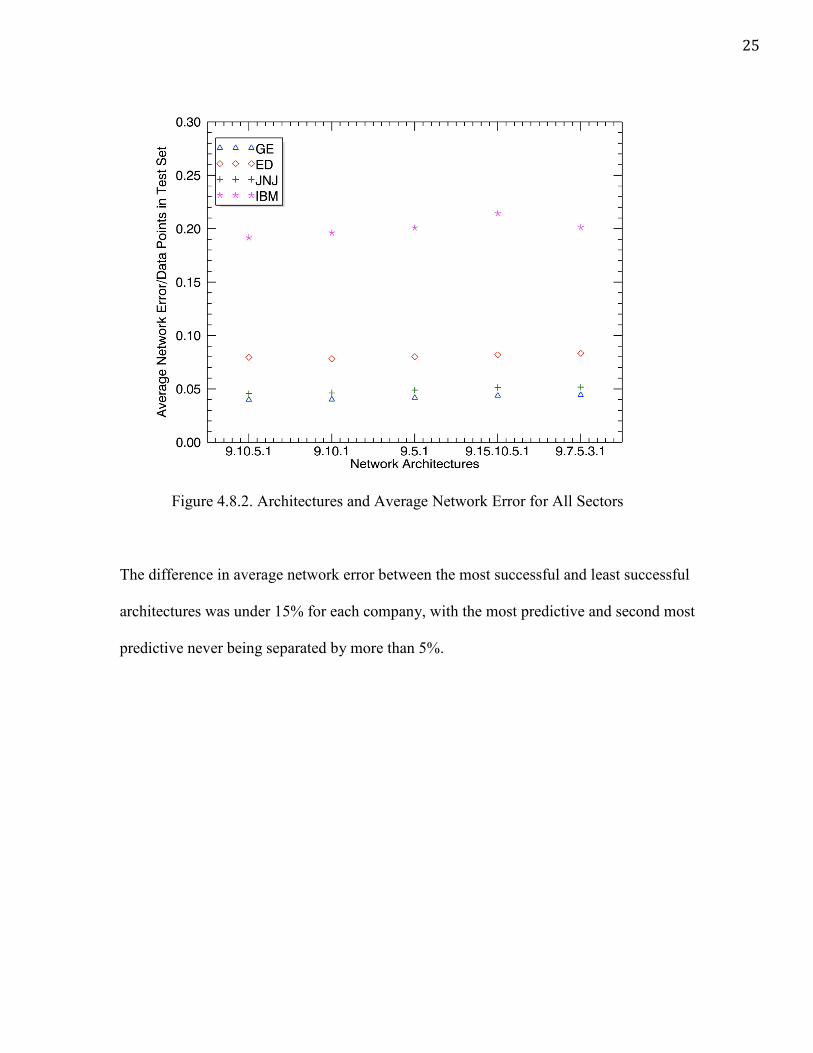
Architecture Avg Net Error/Data Points 9-10-5-1 0.0398 9-5-1 0.04 9-10-1 0.0418 9-15-10-5-1 0.0436 9-7-5-3-1 0.0443

25

Figure 4.8.2. Architectures and Average Network Error for All Sectors

The difference in average network error between the most successful and least successful

architectures was under 15% for each company, with the most predictive and second most

predictive never being separated by more than 5%.

26

5. CONCLUSIONS

5.1. Standard of Success

At the outset of this project, a simple standard was established to measure success - could a

neural network be trained to correctly predict which way a stock would move 51% of the

time? With time, the model shifted away from a network that outputs buy or sell, to one that

attempts to predict the next day’s price. However, while the metrics used to measure the

network’s success were altered, the purpose of the project did not. So, did this network, in the

parlance of the financial press, “beat the Street”?

Conclusions are laid out in six segments, each discussing results from two different angles -

network metrics and monetary values. In order to transition from network metrics (network

error) to monetary value, price data needs to be represented in an unscaled form. Since this

project averaged the absolute values of each network error, by multiplying by the average

network error and the maximum network error of corresponding unscaled Delta prices, we

can obtain the monetary value of the network’s output. In the unscaled Delta GE data set, the

largest recorded price drop was $2.21 and the highest increase was $2.00. Therefore will be

able to examine results using market metrics by multiplying network outputs by $4.41.

5.2. Short Selling

In terms of market metrics, there is one final term to be discussed in order to form a complete

understanding of why this network might be useful. It is also one of the answers to the

question “how can profit be made when a stock declines in value?” Short selling is the sale of

27

a security, which the seller owns, with the hope that the security’s price will decrease, and

the seller will be able to buy it back at a lower price than they sold it, thereby converting the

difference to profit. Predictions of a decline in stock price are just as salient as predictions of

an increase in price [12].

5.3. Scaling

Scaling the data was essential to the success of this project, with non-scaled data being

rejected outright because of refusal to train. A 5.5% decrease in net error from partially

scaled to fully scaled data was observed, as the average network error dropped from 0.046 to

0.0436. Partially scaled, non-delta data, with the most effective maximum error (0.0009)

produced the least predictive recorded results with an average difference between the

network’s guess and the actual price of $0.193 or 0.58% of GE’s June 3 value, the initial

value in the data set, $33.33. Fully scaling data improved average network error by 5.5%, or

$0.009, decreasing the average difference to $0.184.

5.4. Predictors

The 3-day predictor proved to be the most predictive, with the 2-day using less data and

producing a higher average network error, or underfitting, and 4-day exhibiting overfitting. A

7.4% decrease in net error was observed as the average net error dropped from 0.0422 to

0.0393 from 4-day to 3-day predictors. Adding and subtracting days from the predictor

resulted in increased average net errors, pointing towards the 3-day predictor as the optimum

solution. 3-day predictor non-delta data tested with the most effective maximum error,

28

0.0009, yielded an average difference between the network’s guess and the actual price of

$0.165, or 0.49% of GE’s June 3 value.

5.5. Optimal Maximum Error

One third of all testing completed during this project was done on maximum error with 10

different test and training sets being run at each maximum error level. Maximum error testing

successfully produced a consistent minimum average net error, and showed that the average

net error was increased when ME was shifted either up or down from 0.0009. A 3% decrease

in net error was observed as the maximum error decreased from 0.001 to 0.0009, and a 3.5%

increase was observed as the maximum error decreased from 0.0009 to 0.0008. Though the

margins were relatively small, a maximum error of .0009 consistently proved to be most

predictive across all four companies.

5.6. Optimal Network Architectures

Architecture testing was successful, producing two superior architectures, 9-5-1 and 9-10-5-

1. This phase of testing, was largely undertaken at random, as network architectures are

something of a black box. This project acknowledged the probability of more predictive

network architectures, and sought instead to achieve two goals: a) find one or more

architectures that consistently produced the lowest average error over all four sectors and b)

find a group of architectures which had a small difference in average network error from

most to least predictive. 9-10-5-1 produced the smallest network error across all four

companies, with 9-5-1 coming in close second.

29

5.7. Delta

Delta provided the most prominent net error decreases of any method in this project, with net

error decreasing 25.6% (relative to non-delta average network error), a drop of 0.008 from

0.0393 to 0.0313, on fully scaled, 3-day predictor data. Quantified monetarily, the drop

signifies a $0.033 increase in average price predictability, with the average difference

between the network’s guess and the actual next-day price dropping to $0.132. With such a

massive gain in predictive power, it begs the question, are price and PSAR readings mostly

noise? It is possible the real predictive potential, using these metrics, lies in the price

movement history.

5.8. Monetary Analysis

So did the neural network designed by this project beat the Street? GE’s average daily move,

computed by summing the absolute delta prices and dividing by the number of data points,

was $0.234. The optimal network’s guesses averaged an error of only $0.132. Not only could

we reasonably expect the network to predict which way GE would move the following day,

but it would be expected to do so with a whopping 43.6% margin for error (($0.234-

$0.132)/$0.234). Assuming this network was used only to make decisions of whether to

“buy” or “short” GE, the stock’s price movement would have to deviate from the average

43.7% in the wrong direction to illicit an unprofitable choice. The network beat the Street.

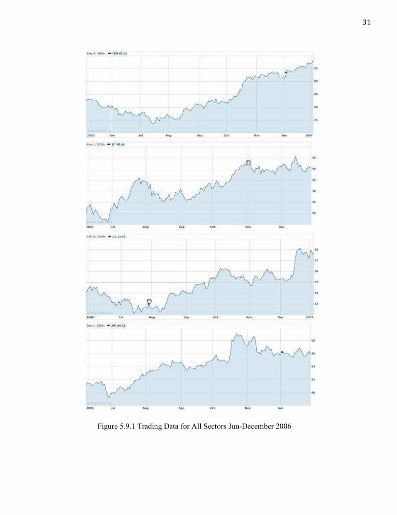
5.9. Trading Patterns

30

Among sectors represented in this project, Industry carried the highest predictability.

Whether this should be attributed to GE’s specific trading patterns or the industry’s tendency

towards following patterns, this project cannot confirm. The Technology sector carried by far

the lowest predictability, with the network outputting an average error of 0.261 on IBM data,

and in fact a network trained to simply output 0.5 for every input combination would have a

lower expected average error (0.25). Below are the trading patterns for all four companies

over the period considered. All four moved higher over the course of 2006 yet, with the

exception of IBM, did so with high degrees of volatility. So why was the net so inept at

predicting IBM’s movements? PSAR and W %R likely played a key role in misinforming the

network to such an extent. That the network even reached its maximum error with such

unsuccessful synaptic weights established, is noteworthy.

31

Figure 5.9.1 Trading Data for All Sectors Jun-December 2006

32

Works Cited

1. Lewis, Michael. The Real Price of Everything: Rediscovering the Six Classics of Economics. New York, NY: Sterling, 2007. Print. 2. Higgins, Adrian. "Tulips Once Caused a Market Crash, but These Days Consumer Confidence Is High." Washington Post. The Washington Post, 30 Apr. 2009. Web. 29 Apr. 2012. <http://www.washingtonpost.com/wp-dyn/content/article/2009/04/29/AR2009042901305>. 2. "CRM: Summary for Salesforce.com Inc Common Stock- Yahoo! Finance." Yahoo! Finance. 01 Mar. 2012. Web. 29 Apr. 2012. <http://finance.yahoo.com/q?s=crm>. 3. "Salesforce.com Market Cap: 21.31B." Salesforce.com Market Cap (CRM). 01 Mar. 2012. Web. 29 Apr. 2012. <http://ycharts.com/companies/CRM/market_cap>. 4. "VIX Options and Futures." CBOE.com. 1 Apr. 2012. Web. 29 Apr. 2012. <http://www.cboe.com/micro/VIX/vixintro.aspx>. 5. Drachman, David A. "Do We Have Brain to Spare?" Neurology. 28 June 2005. Web. 29 Apr. 2012. <http://www.neurology.org/content/64/12/2004>. 6. Haykin, Simon S. Neural Networks and Learning Machines. New York: Prentice Hall/Pearson, 2009. 8. "Williams %R." Definition. Web. 29 Apr. 2012. <http://www.investopedia.com/terms/w/williamsr.asp>. 9. "Parabolic Indicator." Definition. Web. 29 Apr. 2012. <http://www.investopedia.com/terms/p/parabolicindicator.asp>. 10. "Generated Documentation." Java Neural Network Framework Neuroph. Web. 29 Apr. 2012. <http://neuroph.sourceforge.net/javadoc/index.html>. 11. "Iris Classification Dataset Test." Iris1 Neuroph. 02 June 2010. Web. 29 Apr. 2012. <http://sourceforge.net/apps/trac/neuroph/wiki/Iris1>. 12. Fuhrmann, Ryan C. "An Overview Of Short Selling." Investopedia – The Web's Largest Investing Resource. 24 Apr. 2012. Web. 29 Apr. 2012. <http://www.investopedia.com/financial-edge/0412/An-Overview-Of-Short-Selling.aspx>.