pattern-forming in non-equilibrium quantum systems and
TRANSCRIPT

Pattern-forming in
Non-equilibrium Quantum
Systems and Geometrical Models
of Matter
Guido Franchetti
Robinson College
Dissertation submitted for the degree of Doctor of Philosophy
September 2013

Declaration
This dissertation is the result of my own work and includes nothing which is the
outcome of work done in collaboration, except where specifically indicated in the
text. No part of this dissertation has been previously submitted for a degree or
any other qualification.
Guido Franchetti
i

Summary
Pattern-forming in Non-equilibrium Quantum Systems
and Geometrical Models of Matter
Guido Franchetti
This thesis is divided in two parts. The first one is devoted to the dynamics of po-
lariton condensates, with particular attention to their pattern-forming capabilities.
In many configurations of physical interest, the dynamics of polariton condensates
can be modelled by means of a non-linear PDE which is strictly related to the
Gross-Pitaevskii and the complex Ginzburg-Landau equations. Numerical simula-
tions of this equation are used to investigate the robustness of the rotating vortex
lattice which is predicted to spontaneously form in a non-equilibrium trapped con-
densate. An idea for a polariton-based gyroscope is then presented. The device
relies on peculiar properties of non-equilibrium condensates — the possibility of
controlling the vortex emission mechanism and the use of pumping strength as a
control parameter —and improves on existing proposals for superfluid-based gy-
roscopes. Finally, the important role played by quantum pressure in the recently
observed transition from a phase-locked but freely flowing condensate to a spatially
trapped one is discussed. The second part of this thesis presents work done in the
context of the geometrical models of matter framework, which aims to describe
particles in terms of 4-dimensional manifolds. Conserved quantum numbers of par-
ticles are encoded in the topology of the manifold, while dynamical quantities are
to be described in terms of its geometry. Two infinite families of manifolds, namely
ALF gravitational instantons of types Ak and Dk, are investigated as possible mod-
els for multi-particle systems. On the basis of their topological and geometrical
properties it is concluded that Ak can model a system of k ` 1 electrons, and Dk
a system of a proton and k ´ 1 electrons. Energy functionals which successfully
reproduce the Coulomb interaction energy, and in one case also the rest masses, of
these particle systems are then constructed in terms of the area and Gaussian cur-
vature of preferred representatives of middle dimension homology. Finally, an idea
for constructing multi-particle models by gluing single-particle ones is discussed.
ii

Acknowledgements
First and foremost I would like to thank my supervisor Natalia Berloff for her
invaluable support and guidance throughout my PhD and Nick Manton for his
precious advice in so many deeply stimulating discussions. Without their help this
thesis would not have been written.
I could not have gone through the difficult moments of my PhD without the
help of my parents Carlo and Adriana and of my friends.
I am deeply grateful to my girlfriend Maria Alessandra who supported and
encouraged me when I was at my worst.
Finally I would like to thank Marie Curie Actions for financial support, Robin-
son College for its wonderful atmosphere and Cambridge for being such an excep-
tional and inspiring place.
iii

Contents
Declaration i
Summary ii
Acknowledgements iii
Contents iv
1 Introduction 1
I Polaritons 7
2 Background Material 8
2.1 The Physical System . . . . . . . . . . . . . . . . . . . . . . . . . . 8
2.2 A Mathematical Model . . . . . . . . . . . . . . . . . . . . . . . . . 22
2.3 Some Examples . . . . . . . . . . . . . . . . . . . . . . . . . . . . . 32
2.4 Vortices . . . . . . . . . . . . . . . . . . . . . . . . . . . . . . . . . 38
3 Spontaneous Rotating Vortex Lattices and Their Robustness 53
3.1 Vortex Array . . . . . . . . . . . . . . . . . . . . . . . . . . . . . . 54
3.2 Stability Analysis . . . . . . . . . . . . . . . . . . . . . . . . . . . . 57
3.3 Robustness . . . . . . . . . . . . . . . . . . . . . . . . . . . . . . . 65
4 Polariton Gyroscope 74
4.1 The Apparatus . . . . . . . . . . . . . . . . . . . . . . . . . . . . . 74
4.2 Effects of the External Potential . . . . . . . . . . . . . . . . . . . . 77
4.3 The Model in 2D . . . . . . . . . . . . . . . . . . . . . . . . . . . . 81
5 Influence of the Pumping Geometry on the Dynamics 85
5.1 A Quantum Harmonic Oscillator . . . . . . . . . . . . . . . . . . . 85
5.2 Multiple Pumps . . . . . . . . . . . . . . . . . . . . . . . . . . . . . 88
iv

Contents v
II Geometrical Models of Matter 95
6 Background Material 96
6.1 Geometrical Preliminaries . . . . . . . . . . . . . . . . . . . . . . . 96
6.2 Geometric Models of Matter . . . . . . . . . . . . . . . . . . . . . . 101
6.3 Gravitational Instantons . . . . . . . . . . . . . . . . . . . . . . . . 103
7 Asymptotic Topology and Charge 115
7.1 Definition . . . . . . . . . . . . . . . . . . . . . . . . . . . . . . . . 116
7.2 Ak´1 and Dk Charge and Particle Interpretation . . . . . . . . . . 125
8 Geometry and Energy 133
8.1 A Yang-Mills Functional on Ak´1 . . . . . . . . . . . . . . . . . . . 133
8.2 Komar Mass . . . . . . . . . . . . . . . . . . . . . . . . . . . . . . . 139
8.3 Area and Gaussian Curvature of Minimal 2-cycles . . . . . . . . . . 141
9 A Model Under Construction 149
9.1 A Discussion of the Hypotheses . . . . . . . . . . . . . . . . . . . . 149
9.2 Gluing Particles . . . . . . . . . . . . . . . . . . . . . . . . . . . . . 152
9.3 Relations with Kaluza-Klein Theory . . . . . . . . . . . . . . . . . . 156
III Appendices 158
A Polaritons 159
A.1 Excitation Spectrum . . . . . . . . . . . . . . . . . . . . . . . . . . 159
A.2 Madelung Transformation . . . . . . . . . . . . . . . . . . . . . . . 161
A.3 Dimensionless Units . . . . . . . . . . . . . . . . . . . . . . . . . . . 163
A.4 Some Details on the Numerical Techniques . . . . . . . . . . . . . . 165
B Geometric Models of Matter 167
B.1 Topological Invariants . . . . . . . . . . . . . . . . . . . . . . . . . 167
B.2 Equivalence of Charge Definitions . . . . . . . . . . . . . . . . . . . 170
B.3 Principal Bundles, Connection and Curvature . . . . . . . . . . . . 173
B.4 Calculation of R and ||R||2 for Ak´1 . . . . . . . . . . . . . . . . . 182

Chapter 1
Introduction
In this thesis I present work falling into two different areas. The first one is the
dynamics of exciton-polariton condensates, with particular attention to vortex dy-
namics and pattern formation. The second one is the use of ALF (Asymptotically
Locally Flat) gravitational instantons as models for multi-particle systems accord-
ing to the recent geometrical approach to particle physics [6], which I will refer to
as the geometric models of matter framework.
These topics are undoubtedly far apart from each other. Exciton-polariton con-
densates1, briefly polaritons condensates, are 2-dimensional systems characterised
by a high degree of spatial and temporal coherence due to multi-body effects and
the bosonic nature of polaritons. They are non-equilibrium systems since the con-
stituent quasi-particles have a finite lifetime.
The geometric models of matter framework aims to describe the properties
of elementary particles rather then emergent collective behaviour and applies to
systems with few degrees of freedom. Particles are modelled by geometrical ob-
jects, Riemannian 4-manifolds with a particular topology and geometry of which
ALF gravitational instantons are a specific example. Dynamics has not yet been
incorporated in the picture, but is expected to be of conservative relativistic type.
There are, however, some similarities. First, in both cases the system is de-
scribed by a classical field. In the case of polariton condensates, we are inter-
ested in the dynamics of the ground state. Since this is macroscopically occupied,
one can neglect its quantum nature and describe it in terms of a complex-valued
scalar field obeying a partial differential equation similar to the complex Ginzburg-
Landau equation. In the case of ALF gravitational instantons, the relevant field
is the metric tensor.
Second, in both cases we are interested in the study of localised, persistent
structures having a non-trivial topology. In the case of polariton condensates,
we will be interested in the dynamics and pattern-forming properties of vortices.
In the geometrical models of matter framework we will consider manifolds, ALF
1There is some debate on whether the terminology is appropriate, see section 2.1.2.
1

Chapter 1. Introduction 2
gravitational instantons, which model not just particles, but also the empty space
in which the particles reside. These manifolds need therefore to reduce to flat
space at large distances from the particles cores but to have a non-trivial structure
where particles are located.
Both vortices and instantons are examples of topological solitons. In order to
give a precise definition of a topological solitons one needs to refer to a particular
theory. Generally speaking topological solitons are finite energy field configurations
which are solutions of the dynamical equations of the theory and have a topological
structure different from that of the vacuum.2 Energetically cheap modifications of
a given field configuration are localised and cannot change its topology, therefore
solitons cannot decay into simpler structures and exhibit a remarkable stability and
a particle-like behaviour. In order to have a finite energy, the field usually needs
to approach a constant value at large distances, which explains the localisation
properties of solitons. Examples of topological solitons are kinks in 1D, vortices in
2D, monopoles in 3D and instantons in 4D. The qualitative features of topological
solitons are quite independent from the details of the theory.
For non-equilibrium system, it is arguably not correct to use the term soliton.
However, there are structures, for example vortices, which behave very similarly
to their equilibrium counterparts. While a notion of energy is not well defined,
it remains true that in order to destroy a non-trivial topological structure it is
necessary to modify the global, rather then local, configuration of a field. Such
changes do not occur easily and so topological solitons tend to be stable also in
the non-equilibrium context.
The topological solitons which we will be interested in are vortices in polariton
condensates and gravitational instantons. In the case of vortices the non-trivial
topology is due to the fact that the complex scalar field has non-zero winding
number along curves which go around the centre of the vortex. ALF gravita-
tional instantons have generally non-trivial middle dimensions homology groups
and approach asymptotically a non-trivial circle fibration.
There is however a difference between these two areas which is even more dif-
ficult to overcome then those listed so far. The study of polariton condensates
2Sometimes the term soliton is used to denote only finite energy solutions of integrable sys-tems. Following [59] we use the term in its broader acception.

Chapter 1. Introduction 3
was initiated around 2006, when condensation was first achieved [51]. Despite its
youngness, the field has experienced a rapid development, favoured by the rela-
tively high condensation temperature of polaritons and the elevated degree of ex-
perimental control that they offer. Experimental and theoretical advance has been
fast, and the problems investigated have progressed from the mere achievement of
condensation to detailed questions about the behaviour of polariton condensates
under particular trapping or pumping geometries.
On the other hand, the idea of describing particles by means of 4-dimensional
manifolds, while being inspired by older ideas like the Kaluza-Klein model, is nearly
newborn, the first paper having been published in 2012. Moreover, its aim is not
to describe a newly found state of matter, as in the case of polariton condensates,
which lie somewhere in between Bose-Einstein condensates and lasers, but to offer
a new perspective on a subject, particle physics, which already has a theoretical
framework of astonishing precision, quantum field theory. The model has been
proposed not so much to improve on this precision, but rather in the hope that
a different viewpoint could lead to new ideas, provide a better understanding of
what particles are and maybe solve some of the longstanding problems of quantum
field theory.
Different aims call for different methods. In the polariton area my work has
been focused on understanding, mainly by means of numerical simulations, the be-
haviour of polariton condensates in configurations of experimental interest. In my
work on gravitational instantons I have investigated whether two specific families
are appropriate models for multi-particle systems, and I have constructed suitable
energy functionals out of their topological and geometrical properties.
For these reasons, I have decided not to try a parallel treatment of my work in
the two areas, nor to force the use of a common language or of a similar notation,
as I felt that doing so would have obscured the subject and led to no additional
insight. Instead, I have split the thesis in two parts, one devoted to polaritons,
and the other to gravitational instantons.
Having, I hope, justified the division in two parts, let me describe the content of
each one. The first part is concerned with polariton condensates. My own results
are presented in section 3.3, chapter 4 and section 5.2. Chapter 3 discusses the
spontaneous formation of a rotating vortex lattice in a trapped polariton conden-

Chapter 1. Introduction 4
sate and its robustness. This chapter is based on joint work published in [14], which
builds on previous work presented in [52]. My own contribution to [14] has been
the numerical investigation of the robustness of the system against various kinds
of perturbations and is presented in section 3.3. Chapter 4 shows how the suscep-
tibility of polariton condensates to nucleate vortices if some instability threshold
is reached can be used to build an apparatus capable of measuring absolute an-
gular velocities. A preprint illustrating this idea is on the arXiv [35]. Chapter 5
describes joint work published in [26] showing how the behaviour of a polariton
condensate is influenced by the geometry and number of spots at which polaritons
are injected. I have contributed to the theoretical understanding of the system and
performed all the numerical simulations. Chapter 2 contains background material.
The second part is concerned with gravitational instantons. My results are
presented in section 7.2, chapter 8 and chapter 9. Chapter 7 is devoted to the
calculation of the electric charge and to the particle interpretation of ALF Ak´1
and ALF Dk gravitational instantons. Chapter 8 presents various attempts at the
construction of an energy functional for these manifolds. Both chapters are based
on results published in [36] but contain additional material. Chapter 7 includes,
see section 7.1, a thorough explanation of the topological definition of electric
charge. Chapter 8 contains, see sections 8.1 and 8.2, some less successful but still
interesting constructions which were excluded from the published paper. Chapter
9 is devoted to a more general discussion of the current status of the geometric
models of matter framework and of some possible evolutions. Section 9.1 contains
a critical discussion of the hypothesis made in [6]. Section 9.2 presents an idea,
still at a preliminary stage, for building multi-particle systems by gluing together
single-particle ones. Section 9.3 is devoted to a brief comparison with Kaluza-
Klein theory. Chapter 6 contains background material; in particular section 6.2
gives a short review of the geometric models of matter framework as presented in
[6]. Other background material has been put in the appendices.

Chapter 1. Introduction 5
This Thesis in Brief
For reference we give below a short description of the original material presented
in this thesis and, if published, of where it can be found.
Chapter 3: The instability of stationary circularly symmetric solutions of a
modified Gross-Pitaevskii equation, used to model a polariton condensate, against
perturbations carrying angular momentum is proved analytically. The robustness
of the rotating vortex lattice which forms, as predicted in previous work [52], as
a result of this instability is numerically probed against elliptic deformations of
the trap, presence of disorder and changes in the modelling equation. The results
presented in this chapter have been published in [14].
Chapter 4: The idea and basic setup for a polariton gyroscope capable of high-
precision measurements of angular velocities is proposed. The apparatus is based
on the peculiar properties of polariton condensates, namely the easy experimental
control of many of their properties, their susceptibility to vortex formation and
their high condensation temperature. The idea is illustrated by the numerical and
analytical investigation of a simplified 1D model and by numerical investigation of
the full 2D model. A preprint of the material presented in this chapter is available
on arXiv [35].
Chapter 6: As shown in recent experiments, the polariton condensate which
forms if polaritons are injected at different spatial locations arranged along a circle
exhibits very different dynamical behaviours depending on the number of pumps
and the radius of the circle. In particular, as the radius of the circle is increased,
there is a transition from a fully trapped state to a configuration in which the con-
densates forming at different spots are still locked in phase, but polaritons outflow
is observed and the condensate density is concentrated at the edge of the trap.
This chapter illustrates the experimental results and gives a theoretical explana-
tion of the observed behaviour, based on the role played by quantum pressure. The
material presented here is based on a collaboration with the experimental group
of J. Baumberg, and has been published in [26].
Chapter 7: Working within the framework proposed in [6], two infinite families
of 4-manifolds, ALF gravitational instantons of types Ak and Dk, are investigated
as possible models for multi-particle systems. Their electric charge is calculated.

Chapter 1. Introduction 6
For Ak this amounts to computing minus the first Chern number of the asymptotic
circle fibration. For Dk, owing to the fact that the asymptotic fibration is not
oriented, we need to make use of a different but equivalent definition, which in
turn implies that charge can be calculated as minus one half of the first Chern
number of a branched double cover. The particle interpretation of these manifolds
is also discussed. The results presented in chapters 7 and 8 have been published
in [36].
Chapter 8: Geometrical properties of the ALF gravitational instantons intro-
duced in chapter 7 are used to construct energy functionals for the corresponding
multi-particle systems. In particular, an extension of the Komar mass to the Rie-
mannian signature and a Yang-Mills-like functional are first considered, but lead
to energy functionals independent of the particles positions and thus not suitable
to represent interaction energies. Functionals constructed in terms of the area and
the Gaussian curvature of geometrically preferred (minimal area) representatives
of middle dimension homology are then investigated, and shown to successfully
reproduce the Coulomb interaction energies of the corresponding particle systems.
With the exception of the Komar mass and Yang-Mills constructions, the results
presented in this chapter have been published in [36].
Chapter 9: On the basis of the material presented in chapters 7 and 8, some
ideas for future developments, including a construction, still at a preliminary stage,
which could allow to build multi-particle models from single-particle ones making
use of a particular compactification process, are discussed.

Part I
Polaritons
7

Chapter 2
Background Material
This chapter presents some background material on polariton condensates. Sec-
tion 2.1 describes the physical properties of polaritons and briefly discusses the
controversial issue of their Bose-Einstein condensation. The purpose here is not to
give a comprehensive, up-to-date review of the debate, but rather to establish that,
under some conditions, polaritons show enough coherence to allow for a descrip-
tion in terms of a classic complex scalar field ψ. Section 2.2 introduces a partial
differential equation for ψ, closely related to the complex Ginzburg-Landau equa-
tion, which, with minor variations, will be used in chapters 3, 4 and 5 to model
the behaviour of polariton condensates. Section 2.4 reviews some material about
vortices in non-linear fields.
2.1 The Physical System
2.1.1 Polaritons
Excitons-polaritons, shortly polaritons, are quantum superpositions of excitons
and photons. An exciton is a bound system of an electron and a hole, held together
by electromagnetic interactions.
In a semiconductor, an exciton can be created exciting an electron from the
valence band into the conduction band by shining light in resonance with the
transition frequency. The electron leaves a hole, a region of positive electrical
charge, in the valence band, and it is energetically favourable for the electron-hole
pair to form a bound system, an exciton.
The electron-hole pair can recombine by emitting a photon. Therefore there is a
continuous interconversion between excitons and photons. However, since photons
cannot be perfectly confined, they eventually leave the system. Strong coupling
occurs when the exciton-photon interconversion rate is higher than the rate at
which photons escape from the system. In strong-coupling regime, photons and
excitons somehow lose their individual identities, and the appropriate description
8

Chapter 2. Background Material 9
is in term of their quantum superpositions, polaritons.
Polaritons exist in bulk systems, but polariton condensation has only been
achieved with microcavity polaritons. A semiconductor microcavity, see figure 2.1,
consists of two distributed Bragg reflectors, alternate layers of quarter-wavelength
Quantum wells
Bragg reectors
Figure 2.1: Cartoon of a semiconductor microcavity. Bragg reflectors, made ofalternate layers of materials with different dielectric constants (red and yellowparallelepipeds), trap photons (wavy line) inside the cavity. In order to maximiseexciton-photon coupling, bound electron-hole pairs (red and blue dots) are trappedin quantum wells (grey parallelepiped) placed at the antinodes of the photon cavitymodes.
materials with different dielectric constants, which confine photons inside the cav-
ity acting as high-quality mirrors over a limited range of light frequencies. The
better the quality of the cavity, the longer photons are confined, the longer po-
laritons live. For most experimental setups, the lifetime of polaritons is 5–10 ps.
Cavities of an improved quality have been built recently, allowing for lifetimes up
to about 100 ps [67].

Chapter 2. Background Material 10
Photons are confined in the direction transverse to the line joining the two
mirrors, so their transverse wave vector kK is quantised, |kK| “ kK “ 2πNL,
with N an integer and L the transverse length of the cavity. The cavity photons
dispersion relation is then
~ωγ “~cn
b
k2 ` k2K, (2.1)
where n is the refraction index of the material, c is the speed of light, k is the in-
plane wave vector (i.e. the projection of the momentum wave vector on the plane
where polaritons are confined) and k “ |k|. For small k,
~ωγ „ ~ω0 `~2k2
2mγ
, (2.2)
where
ω0 “2πcN
nL, mγ “ 2π~
nN
cL, (2.3)
with mγ the effective mass of the photon. For most materials mγ „ 10´4me, with
me the electron mass. The length L of the cavity, typically a few micrometres, is
chosen so that ω0|N“1 is equal to the frequency needed to excite an electron from
the conduction to the valence band.
Inside the cavity, excitons are confined in quantum wells, quasi-2D potential
wells. In order to maximise exciton-photon coupling, quantum wells are placed at
antinodes of the electromagnetic field, where the density of photons is highest.
The strong screening of Coulomb interactions in semiconductors results in
loosely bound excitons, known as Wanner-Mott excitons, which extend over a
spatial scale larger than the crystal lattice constant. As a consequence, the ef-
fects of the lattice potential on Wanner-Mott excitons can be taken into account
by treating them like free particles with an effective mass mex. The dispersion
relation is then
~ωex “ ε`p2
2mex
, (2.4)
where ε is a constant and p is the exciton momentum. For most materials, mex is
in the range 0.1–1 me, much bigger than the photon effective mass, and ε „ 1.5
eV.
The dispersion relation of polaritons can be found by solving the coupled sta-

Chapter 2. Background Material 11
tionary Schrodinger equation
˜
~ωγ g2
g2 ε
¸˜
ψγ
ψex
¸
“ Euplp
˜
ψγ
ψex
¸
, (2.5)
where g is the interconversion rate between photons and excitons and we have
approximated the excitons energy (2.4) with just the constant term ε. Solving
(2.5) we get
Euplp “1
2
»
–
ˆ
~ω0 ` ε`~2k2
2mγ
˙
˘
d
ˆ
~ω0 ´ ε`~2k2
2mγ
˙2
` g2
fi
fl . (2.6)
Considered as functions of k, Eup and Elp, are usually called the upper polariton
∆
-2 -1 1 2k HΜm
-1L
1.49
1.51
1.53
1.55
E HeVL
Eup
Elp
Eex
EΓ
Figure 2.2: Upper (Eup) and lower (Elp) polariton branches, exciton (Eex) andcavity photon (Eγ) dispersion curves for positive detuning δ. The black dots markthe inflection points in the lower polariton branch. Note how the heavy excitonmass results in a flat exciton dispersion curve. The curves Eup and Elp have beenplotted for the lowest energy transverse photonic modes, i.e. taking N “ 1 in (2.3).For low energy polaritons the contribution of higher N modes can be neglected.
branch and the lower polariton branch, see figure 2.2. The difference Eupp0q ´
Elpp0q “ 2g is known as Rabi splitting. The difference δ “ ~ω0 ´ ε between the
bottom of the photon and exciton dispersion curves is called detuning, and can be

Chapter 2. Background Material 12
positive, negative or zero.
The LP branch has a cavity-photon-like character for low k:
Elp »1
2
„
ε` ~ω0 `~2k2
2mγ
´a
γ2 ` p~ω0 ´ εq2ˆ
1´~ω0 ´ ε
γ2 ` p~ω0 ´ εq2~2k2
2mγ
˙
“ A`Bk2, with
A “1
2p~ω0 ` εq ´
a
γ2 ` p~ω0 ´ εq2,
B “
˜
1`~ω0 ´ ε
a
γ2 ` p~ω0 ´ εq2
¸
~2
2 ¨ 2mγ
.
(2.7)
The effective mass of low-energy polaritons is of the order of the photon mass,
m “ 2mγ „ 2 ¨ 10´4me. (2.8)
For larger |k|, the LP branch has two inflection points, marked with dots in
figure 2.2, where the effective mass of polaritons
m “ ~2
ˆ
B2Elp
Bk2
˙´1
(2.9)
changes sign. This has important consequences on the dynamics, see section 2.2.1
for some discussion.
For high k, the LP branch approaches the exciton dispersion, and the effective
mass of polaritons becomes equal to that of excitons. In a sense, the lower polariton
branch interpolates between photon-like and exciton-like behaviour. More details
on polaritons can be found in [53] and references therein.
2.1.2 To Condense or not To Condense
Polaritons are bound state of photons and spin one excitons and, at low enough
densities1, behave as bosons. Therefore, below some critical temperature, polari-
tons are expected to undergo Bose-Einstein condensation. However the question of
1The density is low enough if nexpa0qd ! 1, where a0 is the Bohr radius and nex the number
density of excitons, and d the dimensionality of the system. If this condition is not satisfied,electrons and holes undergo a Mott transition, unbinding and forming an electron-hole plasma.

Chapter 2. Background Material 13
polariton condensation is not a straightforward one, and is still the object of many
a heated discussion. Here I review some facts about traditional Bose-Einstein
condensation and mention some of the more complicated issues that arise when
considering low-dimensional, non-homogeneous or non-equilibrium systems.
A review of Bose-Einstein condensation
This section presents a quick review of some aspects, focusing on the easiest case:
a 3D system of non-interacting bosons. A good reference for equilibrium Bose-
Einstein condensation is [74].
A 3D non-interacting spatially uniform Bose system (ideal Bose gas) undergoes
Bose-Einstein condensation at the critical temperature
kBTc “2π~2
m
ˆ
n
g32p1q
˙23
, (2.10)
where m is the mass of the Bose gas constituents, n is the number density and
g32p1q „ 2.61 [74]. For T ă Tc, a macroscopic number of particles condenses in the
zero momentum state. For an ideal Bose gas, all the particles are in the condensate
for T “ 0. As we will see, this macroscopic occupation of a single-particle state
allows for a description of the system in terms of a complex scalar field ψpxq.
At the microscopic level, a stationary state of a system of N bosons is described
by the many-body Schrodinger equation
Hpx1, . . . ,xNqψpx1, . . . ,xNq “ E ψpx1, . . . ,xNq, (2.11)
where ψpx1 . . . ,xNq is a many-body wave function and the Hamiltonian H is of
the form
Hpx1 . . . ,xNq “Nÿ
i“1
ˆ
´∇2
i
2m` Vextpxiq
˙
`1
2
ÿ
i‰j
Up|xi ´ xj|qq. (2.12)
Here U is the inter-particle potential and Vext an external potential.
In the second quantisation formalism, an equivalent but often more convenient
description can be given in terms of a quantised field ψpxq [48]. Let |ψENy be an

Chapter 2. Background Material 14
N -particles eigenstate with energy E, and ψENpx1, . . . ,xNq be the corresponding
eigenfunction,
ψENpx1, . . . ,xNq “ xx1 . . .xN |ψENy, (2.13)
with ψENpx1 . . . ,xNq satisfying (2.11). The wave function ψENpx1, . . .xNq can be
expressed in terms of a quantised field ψpxq as
ψENpx1 . . .xNq “1?N !x0|ψpx1q . . . ψpxNq|ψENy. (2.14)
Total symmetry of the wave function under the exchange of two particles is auto-
matically accounted for provided that the field ψpxq satisfies the canonical bosonic
commutation rules,”
ψpxq, ψ:px1qı
“ δpx´ x1q. (2.15)
In the second quantisation formalism, the Hamiltonian H and particle number
N operators are given by
H “
ż
dx ψ:pxq
ˆ
´~2
2m∇2` Vextpxq
˙
ψpxq
`1
2
ż
dx1dx2 ψ:px1qψ
:px2qUp|x1 ´ x2|qψpx2qψpx1q,
(2.16)
N “
ż
dx ψ:pxqψpxq. (2.17)
In writing (2.16) we have assumed that the system is dilute enough to consider only
two-body interactions. Since H and N commute, they admit common eigenstates.
The field ψpxq is a common eigenstate as
”
ψpxq, Nı
“ ψpxq, (2.18)
”
ψpxq, Hı
“
ˆ
´~2
2m∇2` Vextpxq `
ż
dx1ψ:px1qUp|x1 ´ x|qψpx1q
˙
ψpxq. (2.19)
It is convenient to expand ψpxq in terms of a complete system of orthonormal
single-particle wave functions uapxq. For simplicity let us consider the case of a

Chapter 2. Background Material 15
spatially uniform system of free bosons, U “ Vext “ 0. Working in a finite volume,
a cube of side L, and imposing periodic boundary condition, we can take
uapxq “1?L3
exp
ˆ
i
~p ¨ x
˙
, (2.20)
with p “ 2π~ aL, a “ pa1, a2, a3q, ai P N, and expand ψpxq as
ψpxq “1?L3
3ÿ
i“1
8ÿ
ai“0
uapxqaa. (2.21)
The operators aa, a:a have the usual interpretation of annihilation and creation
operators for a particle in the quantum state |ay and satisfy the commutation
rules
”
aa, ab
ı
“
”
a:a, a:
b
ı
“ 0,”
aa, a:
b
ı
“ δa,b, (2.22)
with δa,b “ δa1,b1δa2,b2δa3,b3 . The operator na “ a:aaa counts the number na of
particles in the state |ay.
For a system of free bosons, the particles condense in the ground state |0y.
The average occupation number n0, where denotes the average over the grand-
canonical ensemble, of the ground state is, for T ď Tc, proportional to 1´pT Tcq32
[74]. For T ! Tc, the ground state is macroscopically occupied and, to leading
order, we can neglect all the higher energy states in the expansion (2.21), so that
ψpxq „ u0pxqa0. Moreover,
a0a:
0|ψy “”
a0, a:
0
ı
|ψy ` n0|ψy “ p1` n0q|ψy » n0|ψy “ a:0a0|ψy, (2.23)
having used n0 ` 1 „ n0 as n0 " 1 (macroscopic occupation). Therefore, we
can forget the non-commutativity of a:0 and a0 and treat u0pxqa0 as a complex
scalar field ψpxq, known as the order parameter of the condensate. The reason for
this name is the fact that ψpxq changes from zero to a spatially dependent value
different from zero as T is lowered below Tc, signalling the emergence of an ordered
phase of the system. The word “parameter” in the name “order parameter” is

Chapter 2. Background Material 16
unfortunate since ψpxq is actually a function.
Alternatively, ψpxq can be identified with the statistical average of ψpxq in
the grand-canonical ensemble. Since the averaging procedure involves taking the
expectation value of ψpxq over states with a different number of particles, one
would expect it to be zero. The fact that it does not vanish is ultimately due to
the spontaneous symmetry breaking of the Up1q gauge invariance of the theory
(the conserved quantity associated with this gauge invariance being the particle
number), and a signature of the presence of a condensate, see [48] for more details.
The fact that a macroscopic portion of the system is described by a single
wave function results in high spatial and temporal coherence. For example, the
off-diagonal density matrix element
ρ1px,x1q “ ψ:px1qψpxq (2.24)
approaches a finite nonzero value in the limit |x´ x1| Ñ 8, a phenomenon known
as long-range order.2
For simplicity we have discussed the case of a gas of free bosons, but the
analysis can be extended to more complicated systems. For example, a system
of weakly interacting bosons still shows long-range order and accumulates in a
single-particle state at a finite non-zero temperature. However, the quantitative
details are different, for example even at T “ 0 not all the particles are in the
condensate.
Let us now derive the equation of motion for the order parameter of a system of
weakly interacting bosons, which we will need later. Abusing notation, we denote
the field operator ψpxq in the Heisenberg picture by ψpx, tq. It evolves according
to the equation
i~Bψpx, tq
Bt“
”
ψpx, tq, Hı
. (2.25)
2The averaging process is quite subtle because of the spontaneous symmetry breaking. Inorder to evaluate (2.24) it is necessary to couple the system to an external field and take firstthe thermodynamic limit and then the limit of the external field going to zero. The situation issimilar to what happens in the case of the spontaneous magnetisation of a ferromagnet.

Chapter 2. Background Material 17
Using (2.19),
”
ψpx, tq, Hı
“
ˆ
´~2
2m∇2` Vextpxq `
ż
dx1ψ:px1, tqUp|x1 ´ x|qψpx1, tq
˙
ψpx, tq
(2.26)
As we have seen, for a condensate we can replace ψpx, tq with its average, the
classical field ψpx, tq. Because interactions are weak, in (2.16) we can replace the
two-body potential Up|x1 ´ x2|q with the hard-sphere one g δp|x1 ´ x2|q. The pa-
rameter g is related to the s-wave scattering length a by the relation g “ 4πa~2m.
The equation of motion for ψpx, tq is then
i~Bψpx, tq
Bt“
„
´~2
2m∇2` Vextpxq ` g|ψpx, tq|
2
ψpx, tq, (2.27)
known as the Gross-Pitaevskii equation (GPe), or as the non-linear Schrodinger
equation. Alternatively, we could have obtained GPe by replacing the quantum
commutator in (2.25) with the classical Poisson brackets.
The Problem of Condensation for Polaritons Systems
In more complicated cases there are a number of issues to be taken into account.
They have to do with the dimensionality of the system, spatial inhomogeneities
and non-equilibrium.
The Coleman-Mermin-Wagner theorem [25, 60] states that no spontaneous
symmetry breaking can occur at T ą 0 in an infinite homogeneous system of
dimension D which has a continuous symmetry if D ď 2. The reason is that for
D ď 2 fluctuations of the massless modes associated with the broken symmetry
(Goldstone modes) have infrared divergences which destroy long-range order.
However in a homogeneous 2D system a different kind of order is possible. In
fact, as the temperature is lowered, there is a transition, the Berezinskii-Kosterlitz-
Thouless (BKT) transition [11, 55], from a state populated by unbound vortices3
to a state where vortices form tightly-bound pairs. In the lower temperature phase
the system exhibits quasi-long-range order, that is a power-law decay of the off-
3Above a certain temperature creation of vortices becomes favourable as it lowers the freeenergy of the system.

Chapter 2. Background Material 18
diagonal single-particle density matrix at large distances.
The behaviour of an inhomogeneous system can be very different. For example,
a trapped non-interacting 2D Bose system undergoes Bose-Einstein condensation
at a non-zero temperature [8]. The interacting case is particularly complicated
and not totally understood, see [75] for more details.
All the issues that we have mentioned are relevant in the case of polariton
condensates which are 2D interacting systems, generally inhomogeneous. Inho-
mogeneities can be due to trapping potentials, disorder, or finite-size effects. To
further complicate the situation, the finite lifetime of polaritons prevents the sys-
tem from reaching a complete thermal equilibrium.
In order to consider the thermalisation problem, we need first to briefly discuss
how polariton condensates are created in experiments. Of the various possible tech-
niques [53], we are interested in the incoherent or non-resonant pumping, where
a population of hot excitons is created by shining a laser on the microcavity. In
the cooling down process, excitons undergo multiple exciton-exciton and exciton-
phonon scattering events, totally losing coherence. Above some power threshold,
the system enters the strong-coupling regime and the rate of creation of new polari-
tons exceeds the loss rate due to photons escaping from the system. A polariton
population then builds up and subsequently cools off and condenses. Since the
initial polariton population is incoherent, any coherence developed by the system
must be the result of the condensation process.
In order for the condensate to form, the exciton population needs to lower its
temperature, a process known as cooling, and to establish a uniform temperature, a
process known as thermalisation. Both processes take place via polariton-polariton
and polariton-other-particles, notably phonons, interactions. Because of energy
and momentum conservation, only phonons with very low energies can be emitted
in the process, and the time needed to obtain a thermal distribution is longer
then the lifetime of polaritons. This leads to an accumulation of polaritons at the
inflection points of the LP branch, where the spectrum changes from exciton-like
to photon-like, and to a very non-thermal polariton distribution.
Experimental and theoretical progress [31, 58] showed that higher polaritons
densities combined with a slight positive detuning (which makes polaritons in the
LP branch more exciton-like) increases the efficiency of polaritons interactions

Chapter 2. Background Material 19
leading to a faster thermalisation process. Overcome the thermalisation problem,
polariton condensation, intended as macroscopic occupation of a single-particle
state and long-range spatial coherence, see figures 2.3 and 2.4, was first obtained
in 2006 [51].
Figure 2.3: This is image is taken from [51]. It shows the far field emission atT “ 5 K within an angular cone of ˘23˝ at different pump powers. From leftto right, the values are 0.55Pth, Pth and 1.14Pth, where Pth “ 1.67 kW cm´2 isthe threshold power. As the pumping power exceeds Pth an intense peak buildsup in the centre of the emission distribution, corresponding to the zero in-planemomentum state.
Looking at figures 2.3, 2.4, and at similar results from other experiments, it is
evident that the system undergoes some kind of transition, but there is much room
for discussion regarding the precise nature of the transition and whether or not the
resulting system should be called a Bose-Einstein condensate [17]. In fact, Bose-
Einstein condensation is a property of equilibrium systems and is defined in terms
of equilibrium statistical mechanics averages. While condensed polaritons are in
thermal equilibrium among themselves, they coexist with a thermal bath of non-
condensed excitons which have a different temperature. Therefore, in contrast
with equilibrium condensates, it is not possible to define a temperature for the
whole system.
To a certain extent, this controversy is a matter of terminology. While for equi-
librium condensates a number of properties, among which high spatial and tempo-

Chapter 2. Background Material 20
Figure 2.4: This image is taken from [51]. Each point x “ px, yq in the con-tour plots gives the value of the first order correlation function gp1qpx,x1q “ψ˚pxqψpx1q
a
ψ˚pxqψpxqψ˚px1qψpx1q. The left panel is below threshold, the rightpanel above threshold. An increase in the correlation is evident.
ral coherence, quantised vortices, superfluid behaviour4, are equivalent or strictly
related, and can be used to define what a condensate is, in the non-equilibrium
scenario the relations between these properties are much more subtle.
Following common use, I refer to polariton systems exhibiting properties similar
4According to Landau’s criterion, see e.g. [74], the critical speed uc at which excitations startto form and superfluidity breaks down is
uc “ limkÑ0
Re
ˆ
ωpkq
k
˙
where ωpkq is the dispersion relation for excitations of the condensate. A non-interacting Bose-Einstein condensates shows no superfluid behaviour since its dispersion relation is parabolic,ωpkq “ ~2k22m. However, a system of weakly-interacting bosons has the following dispersioncurve, known as the Bogoliubov dispersion,
ωpkq “
d
gρ~2
m2k2 `
ˆ
~2k2
2m
˙2
,
which for small k is phonon-like: ωpkq »?gρ ~ km. Therefore a system of weakly-interacting
bosons flowing at a low enough velocity exhibits superfluid behaviour.

Chapter 2. Background Material 21
to those discussed in [51] as polariton condensates. This does not mean that
some particular definition of non-equilibrium Bose-Einstein condensation has been
chosen. In the end, what matters for this work is the fact that the system exhibits
a degree of coherence high enough to allow for a description in terms of a complex
scalar field obeying some partial differential equation.

Chapter 2. Background Material 22
2.2 A Mathematical Model
The discussion of polariton condensates dynamics in chapters 3, 4, 5 is based on
numerical and analytical study of the following partial differential equation,
i~p1` iηqBtψ “ ´~2
2m∇2ψ ` Vextψ ` g|ψ|
2ψ ` ipΓ´ κ|ψ|2qψ. (2.28)
The general form of (2.28) is Schrodinger-like, i~ Btψ “ Eψ, where ψ is a
complex scalar field, measuring the coherence properties of the system. As al-
ready discussed, the kinetic energy of low-momentum polaritons is proportional
to ´∇2ψ. Polariton-polariton interactions, due to their excitonic component, are
taken into account by the non-linear term g|ψ|2ψ, with g ą 0 since the interac-
tions are of a repulsive nature. The function Vext represents either an externally
imposed potential, e.g. a harmonic trap used to confine the condensate, or natu-
rally occurring disorder. The additional terms in (2.28) are needed to take into
account the non-equilibrium properties of polariton condensates. The quantities
Γ, κ are positive constants, or, for inhomogeneous pumping, positive functions,
which represent the linear and non-linear loss. The parameter η is a positive con-
stant which is introduced to partially account for the interaction of the condensate
with the exciton reservoir, and m is the effective polariton mass. In section 2.2.1
equation (2.28) is interpreted as a Gross-Pitaevskii equation, which, as we have
seen in section 2.1.2, models the behaviour of equilibrium condensates for T ! Tc,
modified so to take into account the finite lifetime of polaritons.
The boundary conditions to be imposed on solutions of (2.28) depend on the
form of Vext, which determines whether the condensate is trapped or not, and
on the spatial dependence of Γ. In a region where Γ vanishes ψ has to decay
to zero. At large distances for a trapped condensate ψ approaches zero, for a
free condensate |ψ|2 approaches its equilibrium value given by, see section 2.2.1,
pΓ´ ηµqκ.
The squared modulus and the gradient of the phase of the complex field
ψ “ |ψ| exppiφq have an important physical interpretation, being related to the

Chapter 2. Background Material 23
density ρ and the velocity u of the condensate,
ρ “ m|ψ|2, u “~m∇φ. (2.29)
A stationary solution of (2.28) has the form
ψpx, tq “ ψpxq exp´
´iµ
~t¯
, (2.30)
where, with abuse of notation, we have denoted with the same symbol both the
time-dependent wave function and the spatial part of the stationary one. The
positive constant µ is the chemical potential of the system. The equation satisfied
by a stationary solution is
µp1` iηqψ “ ´~2
2m∇2ψ ` Vextψ ` g|ψ|
2ψ ` ipΓ´ κ|ψ|2qψ. (2.31)
With the exception of section 2.2.1, from now on we shall mainly work with
the dimensionless form of these equations. With the choice of units described in
appendix A.3 we have ρ “ |ψ|2, u “∇φ and (2.28), (2.31) become
2ip1` iηqBtψ “´
´∇2` Vextpxq ` |ψ|
2` ipα ´ σ|ψ|2q
¯
ψ, (2.32)
µp1` iηqψ “´
´∇2` Vextpxq ` |ψ|
2` ipα ´ σ|ψ|2q
¯
ψ. (2.33)
It is sometimes convenient to recast equation (2.32) in terms of the physical
quantities u and ρ performing what is known as a Madelung transformation. All
one needs to do is to write ψ “?ρ exppiφq and expand the various terms, see
appendix A.2 for the explicit calculation. The result is the system of equations
Btρ`∇ ¨ pρuq ´ 2ηρ Btφ “ pα ´ σρq ρ, (2.34)
2Btφ` η Bt log ρ “ ´u2´ ρ´ Vext `
1?ρ∇2?ρ. (2.35)

Chapter 2. Background Material 24
For a stationary system, Btρ “ 0, 2Btφ “ ´µ and we obtain
∇ ¨ pρuq “ pα ´ σρ´ ηµqρ, (2.36)
µ “ u2` ρ` Vext ´
1?ρ∇2?ρ. (2.37)
For η “ 0, equations (2.34), (2.35) are very similar to the continuity and
Euler equations for a compressible inviscid fluid [76]. In particular, (2.34) is the
continuity equation in the presence of a source αρ and a sink σρ2 and (2.35) is,
but for the last term, the integrated form of the Euler equation for a compressible
fluid whose equation of state is p “ ρ24, p being the pressure of the fluid, see
appendix A.2.5 The term
´1?ρ∇2?ρ (2.38)
has no classical analogue and is known as quantum pressure. It is negligible pro-
vided that the density profile is sufficiently smooth. To be more quantitative, if L
is the length scale of density variations, the quantum pressure term scales as L´2
and it is negligible provided that L " λ, where
λ “1?ρ, (2.39)
known as healing length6, is the length scale over which the condensate density, if
perturbed from its equilibrium value by some obstacle, “heals back” to its unper-
turbed value.
In modelling the behaviour of polariton condensates by means of the single
equation (2.28), several simplifying assumptions have been made. The temperature
needs to be much lower than the critical temperature for condensation Tc. Note
however that for polariton condensates Tc is much higher than for equilibrium
condensates: looking at equation (2.10), we see that Tc is proportional to the
inverse mass of the condensate constituents. For realistic densities, the small mass
of polaritons, m „ 10´4me, gives a critical temperature of 1–10 K, to be compared
with the critical temperature of traditional condensates which is around 100 nK.
5In dimensional units p “ gρ2p2m2q.6In dimensional units λ “ ~
?2gρ.

Chapter 2. Background Material 25
We have ignored the dynamics of the reservoir excitons, but we have taken
some of its effects into account through the phenomenological parameters α, de-
scribing the gain due to excitons condensing into polaritons, and η, describing
the interaction of the condensate with the excitonic reservoir. As we shall see in
section 2.2.1, explicitly including the dynamics of the reservoir would have lead
us, under the physically reasonable assumption of fast reservoir relaxation, to the
same equation.
We have approximated the kinetic energy of polaritons with the simple expres-
sion Epkq “ ´k2, which corresponds to the differential operator ∇2. Looking at
(2.7), we can see that this approximation is valid for low momenta polaritons. The
correct form of the differential operator for higher k polaritons can be found by
Fourier transforming the full dispersion curve (2.6).
We have neglected the polariton polarisation, which is inherited from their pho-
tonic component. While there are cases in which polarisation plays an important
role [82], in most experimental setups mechanical strain in the sample favours lin-
ear polarisation, the phases of left- and right-polarised polaritons becomes locked
and the polarisation degree of freedom can be ignored.
As we can see, the approximations made in describing the system by means of
equation (2.28) do not particularly restrict the range of possible applications, and
indeed (2.28) describes well the dynamics of polariton condensates under a wide
range of experimental conditions without introducing unnecessary complications.
In the next section, we show how (2.28) can be derived starting from two different
viewpoints, explain in more detail the meaning of the various terms, and comment
on its relations with other equations.
2.2.1 Derivation of the Equation
A Modified Gross-Pitaevskii Equation
Polariton condensates are a peculiar kind of Bose-Einstein condensates, so let us
start with the Gross-Pitaevskii equation (2.27), which we rewrite here for reference,
i~Btψ “ ´~2
2m∇2ψ ` Vextψ ` g|ψ|
2ψ. (2.40)

Chapter 2. Background Material 26
As we have already mentioned, (2.40) describes equilibrium condensates at T ! Tc,
so it should be possible to describe polariton condensates modifying the GPe so
to take into account their non equilibrium properties.
The most important change is the introduction of a gain/loss mechanism which
accounts for the finite lifetime of polaritons. The simplest term describing gain or
loss has the form
Btψ “ Γψ, (2.41)
where Γ represent the gain rate minus the loss rate. However, such a term alone
would lead to trivial dynamics: an unbounded growth of the condensate if Γ ą 0
or a disappearance of the condensate if Γ ă 0.
On physical grounds, it is evident that at some point the gain saturates and
that the combined action of gain and loss drives the condensate density towards a
finite value. The simplest way of modelling this behaviour, first proposed in [52],
is to introduce a non-linear loss term ´κ |ψ|2ψ,
Btψ “ pΓ´ κ|ψ|2qψ, (2.42)
with Γ, κ ą 0. Multiplying (2.42) by ψ˚ and adding the Hermitian conjugate we
obtain
Btn “ 2pΓ´ κnqn, (2.43)
where n is the number density of the condensate. We see that the combined effect
of Γ and κ is to drive the condensate towards an equilibrium density neq “ Γκ.
In experiments, pumping is often not extended to the whole system. To model
this aspect, we replace the constant parameters Γ and κ with spatially dependent
functions.
Finally, it is possible to partially account for the relaxation process due to the
interactions between the condensate and the excitonic reservoir via the substitu-
tion,
i~Btψ Ñ ~ pi´ ηq Btψ, (2.44)
with η a positive dimensionless constant [89, 90]. It can be easily checked that a
nonzero η changes the value of the equilibrium density to neq “ pΓ´ ηµqκ.
Putting all these changes together we recover equation (2.28). If the system

Chapter 2. Background Material 27
is at temperatures low enough to neglect interactions with the thermal cloud one
can take η “ 0. For η “ Γ “ κ “ 0 (2.28) reduces to GPe (2.40). For small values
of these parameters, it is possible to study (2.28) by considering perturbative
corrections to the GPe.
Fast Reservoir Relaxation
Another possibility is to start with a coupled system of equations describing the
condensate and the reservoir. However, we will see that, in the assumption of fast
reservoir relaxation, we can reduce the system to the single equation (2.28).
A coupled model for the condensate and the reservoir has been introduced in
[88]:
iBtψ “
„
´~
2m∇2` g|ψ|2 `
i
2pRpnRq ´ γq ` 2g nR
ψ, (2.45)
BtnR “ P ´ γR nR ´RpnRq|ψ|2`D∇2nR. (2.46)
In (2.45) γ is the decay rate of condensed polaritons, nR is the number density of
reservoir excitons, RpnRq is the gain rate of condensed polaritons due to stimulated
scattering from the reservoir into the condensate, g is the strength of condensed
polaritons self-interactions and g is the strength of interactions between condensed
polaritons and reservoir excitons. In (2.46) P is the pumping rate of excitons in
the reservoir, γR is the reservoir decay rate, RpnRq|ψ|2 represents the loss due to
stimulated scattering from the reservoir into the condensate and D is the diffusion
rate of reservoir polaritons. The diffusion constant D is very small [88] and for
simplicity we set it to zero. The function RpnRq is a monotonically growing func-
tion of the reservoir density nR and at leading order is given by Rpnq „ RRnR.
The system (2.45), (2.46) constitutes a quite universal model for a quantum system
coupled to an external reservoir provided that any coherence between the quantum
system and the reservoir is dissipated over time scales which are fast compared to
those on which the quantum system dynamics takes place.
In the limit of fast reservoir relaxation γR " γ the reservoir dynamics is much
quicker than that of the condensate. Therefore the condensate sees a reservoir

Chapter 2. Background Material 28
with a constant density nR given by
nR “P
γR `RR |ψ|2„
P
γR´PRR
γ2R
|ψ|2. (2.47)
Substituting (2.47) in (2.45) we obtain the equation
iBtψ “”
´~2
2m∇2`i
2
ˆ
RRP
γR´ γ
˙
` 2pgR ` gqP
γR´i
2
ˆ
RR
γR
˙2
P |ψ|2
`
ˆ
g ´ 2pgR ` gqPRR
γ2R
˙
|ψ|2ı
ψ.
(2.48)
Setting
α “1
2
ˆ
RRP
γR´ γ
˙
, σ “1
2
ˆ
RR
γR
˙2
P, g “ g ´ 2pgR ` gqPRR
γ2R
, (2.49)
and performing the gauge transformation ψ Ñ ψ exp p´2i pgR ` gqP tγRq we re-
cover (2.28) for η “ 0.
Note that for sufficiently high values of P the sign of g in (2.49) can change from
positive to negative, corresponding to a change in polariton-polariton interactions
from repulsive (g ą 0) to attractive (g ă 0). Physically what happens is that
an increase in the pumping power populates regions of the lower polariton branch
beyond the inflection point, where polaritons effective mass (2.9) becomes negative.
A change in the sign of the effective mass m has the same effects as a change in the
sign of the interaction strength g. This is a well-known phenomenon in the case of
GPe which has very different solutions depending on whether mg ą 0 (defocusing)
or mg ă 0 (focusing). In 1D and for Vext “ 0 the defocusing (focusing) GPe
admits exact solutions describing travelling dips (peaks) in density, called dark
solitons (bright solitons), see for example [16]. While the behaviour of polariton
condensates is deeply affected by the presence of spatial inhomogeneities and by
the dissipative nature of the system, there is a similar distinction between focusing
and defocusing dynamics: while dark solitons are normally observed [2], beyond
some threshold in pumping power bright solitons are emitted [83].

Chapter 2. Background Material 29
2.2.2 Values of the Parameters
In most experiments, the maximum pumping power is around ten times the thresh-
old pumping power, which occurs for zero effective linear gain, Γ “ 0, i.e. equal
linear gain and loss. The linear loss rate can be estimated from the polariton
lifetime τ „ 5 ps as ~τ “ 0.13 meV. With our choice of dimensionless units
α “ 2Γp~ωq, where, for a trapped condensate, ω is the frequency of the trap,
usually of the order of some tenth of a meV. Therefore, α is generally in the range
0 – 10. The value of σ can be estimated from the dependence of the blue-shift on
the pumping power giving σ „ 0.3 [52]. Finally the phenomenological parameter
η is a small quantity η „ 0.1.
2.2.3 Relation with Other Equations
If Vext “ 0 and α, σ, η are constant, equation (2.28) is the complex Ginzburg-
Landau (cGLe) equation, see [3] for a review, in disguise. In fact, performing the
transformations
t “2
α
`
1` η2˘
t1, x “
c
η
αx1, ψ “
c
α
η ` σψ1 exp p´i η t1q (2.50)
we obtain, omitting primes,
Btψ ““
1` p1` ibq∇2´ p1` icq |ψ|2
‰
ψ, (2.51)
which is the cGLe in the standard rescaled form. The parameters b and c are
related to η and σ by
b “1
η, c “
1´ ση
σ ` η. (2.52)
The cGLe models a vast variety of phenomenas, ranging from non-linear waves
to second-order phase transitions, superfluidity and cosmic strings. In fact it ap-
plies to any out-of-equilibrium system which is homogeneous and isotropic, and
which presents a supercritical phase transition described by a complex order pa-
rameter ψ with gauge group Up1q.

Chapter 2. Background Material 30
The dynamics described by cGLe is very different depending on whether b “ c
or b ‰ c. In the first case, rescaling ψ Ñ ψ exp p´ib tq one obtains
Btψ “ p1` ibq`
1`∇2´ |ψ|2
˘
ψ. (2.53)
Equation (2.53) can be obtained by varying the functional7
E “ż„
∇ψ˚ ¨∇ψ `1
2
`
1´ |ψ|2˘2
d2x, (2.54)
Bψ
Bt“ ´p1` ibq
δEδψ˚
. (2.55)
Since, for any finite value of b, the quantity
BtE “δEδψBtψ `
δEδψ˚
Btψ˚“ ´
2
1` b2
ż
|Btψ|2 d2x (2.56)
is negative, the value of E decreases with time. Dynamics is therefore of the
dissipative type and E plays the role of a generalised free energy.
In the particular case b “ c “ 0 one obtains the real Ginzburg-Landau equation
Btψ “`
1`∇2´ |ψ|2
˘
ψ, (2.57)
which is the gradient-flow dynamics generated by the functional E .
In the opposite limit8 b, c Ñ 8, the functional E is conserved and represents
the energy of the system. The corresponding field equation is the Gross-Pitaevskii
7Even if b ‰ c one can obtain the cGLe from a complex functional,
Bψ
Bt“ ´
δEδψ˚
,
with
E “ p1` ibq∇ψ ¨∇ψ˚ ´ |ψ|2 `1
2p1` icq|ψ|4.
However E is neither conserved nor monotonically decreasing.8The limit should be taken in the non-rescaled form of the complex Ginzburg-Landau equa-
tion.

Chapter 2. Background Material 31
equation (2.27) in the absence of any external potential,
Btψ “ ´i`
´∇2˘ |ψ|2
˘
ψ. (2.58)
The non-linear term can have both signs. The plus sign arises if there are repulsive
interactions, and (2.58) with the plus sign is known as the defocusing non-linear
Schrodinger equation. The minus sign arises if there are attractive interactions,
and (2.58) is then called the focusing non-linear Schrodinger equation.
Btψ “ ´i`
´∇2` V ˘ |ψ|2
˘
ψ. (2.59)
Equation (2.28), which we use to model the dynamics of polariton condensates,
is strictly related to the b ‰ c cGLe, but breaks spatial homogeneity because of
the presence of an external potential and, in the case of non-uniform pumping,
spatially dependent coefficients. If these spatially dependent terms are weak or
nearly constant then the cGLe approximates very well the dynamics described by
(2.28). However in most cases the behaviour of the system is dominated by these
spatially dependent effects and dynamics, while deeply modified by pumping and
decay, is better approximated by the GPe.

Chapter 2. Background Material 32
2.3 Some Examples
2.3.1 The Thomas-Fermi Solution
In the study of a polariton condensate it is often useful to treat pumping and decay
as perturbations to the equilibrium dynamics described by the GPe (2.40). Note
that σ, η ă 1, but usually α ą 1. However while perturbation techniques might
fail, understanding the usually simpler behaviour of the equilibrium system often
gives some insight into what happens in the non-equilibrium case.
In the absence of a trapping potential we expect the ground state of the system
to have uniform density. A Madelung transformation of the stationary GPe with
Vext “ 0 gives the system
∇ ¨ pρuq “ 0, (2.60)
µ “ ρ` u2´
1?ρ∇2?ρ, (2.61)
which is solved by
ρ “ µ “ const, u “ 0. (2.62)
If there is a trapping potential Vext which does not vary appreciably over length
scales of the order of the healing length (2.39) we can neglect the quantum pressure
term and consider the system
∇ ¨ pρuq “ 0,
µ “ ρ` u2` Vext.
(2.63)
The Thomas-Fermi solution is given by
ρTF “
$
&
%
µ´ Vext if µ´ Vext ě 0,
0 otherwise,
uTF “ 0.
(2.64)
Let us see what happens if we introduce pumping and decay. For simplicity,
Chapter 2. Background Material 33
we take α, σ and η to be constant. The system
∇ ¨ pρuq “ pα ´ σρ´ ηµqρ, (2.65)
µ “ ρ` u2´
1?ρ∇2?ρ. (2.66)
still has a solution with u “ 0 everywhere:
ρ “ µ “α
σ ` η, u “ 0. (2.67)
In the absence of a trapping potential the equations for an equilibrium and
a non-equilibrium condensate have similar solutions, compare (2.62) with (2.67).
However, the situation changes if we include a trapping potential. In fact it is easy
to see that if we add a spatially varying term Vext to the right-hand side of (2.66)
there can be no solution of the system with u “ 0.
2.3.2 Rotationally Symmetric Potentials
Consider now systems with a rotationally symmetric potential Vextprq depending
only on the radial variable r “a
x2 ` y2. It is convenient to use the polar coordi-
nates pr, θq. The velocity of the condensate is then u “ ur Br ` puθrq Bθ. Because
of the rotational symmetry, uθ vanishes and ρ, ur are functions of r only. Using
∇f “Bf
BrBr `
1
r
Bf
BθBθ,
∇ ¨ v “BvrBr`vrr`
1
r
BvθBθ
,
∇2f “B2f
Br2`
1
r
Bf
Br`
1
r2
B2f
Bθ2,
(2.68)
we can write Madelung equations (2.34), (2.35) in the form
∇ ¨ pρuq “ ρ1 u` ρ u1 `ρu
r“ pα ´ σρ´ ηµq ρ, (2.69)
µ “ ρ` u2` Vext ´
1
2ρ
˜
ρ2
´
`
ρ1˘2
2ρ`ρ1
r
¸
, (2.70)
Chapter 2. Background Material 34
having set ur ” u and 1 “ ddr.
Let us assume that Vextprq varies on length scales large enough to neglect
quantum pressure, the last term in (2.70). In the equilibrium case, α “ σ “ η “ 0,
one has the Thomas-Fermi solution (2.64),
ρTF prq “
$
&
%
µ´ Vextprq if r ď rTF ,
0 otherwise,
uTF prq “ 0.
(2.71)
The smallest solution of the equation µ “ Vextprq, is the Thomas-Fermi radius rTF .
Let us now compare (2.71) with the non-equilibrium solutions for two particular
choices of Vext.
Localised Potential
Take
Vextprq “ V0 exp`
´prr0q2˘
, (2.72)
with V0, r0 positive constants. Let us examine the system at the points r “ 0 and
r “ 8,
r “ 0 r “ 8
u0 “ 0 by symmetry, Vext “ 0, (2.73)
µ “ ρ0 ` V0 pα ´ σρ8 ´ ηµq ρ8 “ 0.
where ρ8 ” limrÑ8 ρprq. Since the potential approaches zero at large r, the
condensate is not trapped and we expect to have non-vanishing density and velocity
at infinity. The quantity ρ ` u2 ` Vext is constant and Vext decreases with r, so
we expect u and ρ to be monotonically increasing functions taking the asymptotic
values ρ8 “ pα´η u28qpσ`ηq and u8 “
a
µpσ ` ηqσ ´ ασ. These expectations
are confirmed by the results of numerical simulations, see figure 2.5. As shown in
figure 2.6, for a potential with a smaller length scale r0 the contribution of quantum
pressure cannot be neglected.
Note that (2.69), (2.70) is a system of two equations in the two unknown func-

Chapter 2. Background Material 35
-15 -10 -5 5 10 15
5
10
15
Ρ
u
Vext
q. p.
Μ
Ρ¥
ΡTF
Figure 2.5: Plot of ρ, u2, Vext, q. p. (quantum pressure) and of their sum µ (blackline). Note that µ is, as it should be, constant. The length scale r0 “ 4 ofthe potential, is much bigger than the healing length, therefore quantum pressure(orange line) is totally negligible. The asymptotic value of the density, ρ8 “ ασand the equilibrium Thomas-Fermi solution ρTF are also shown. The parametersused in the simulation are σ “ 0.3, α “ 4, η “ 0.
-2 -1 1 2
-5
5
10
15
Ρ
u
Vext
q. p.
Μ
Ρ¥
ΡTF
Figure 2.6: Same plot as in figure 2.5, but for r0 “ 0.4. Note that quantumpressure is different from zero over a length which is approximately twice r0.

Chapter 2. Background Material 36
tions ρ and u which are therefore generally determined in terms of the parameters
µ, α, σ, η. While α, σ and η are to be considered as given, the chemical potential
µ is not. For an equilibrium condensate, µ can be found by using the fact that the
total particle number is conserved. In the non-equilibrium case there is no general
procedure for finding µ but, provided that quantum pressure is negligible, its value
can be obtained by using equation (2.70) if one knows the value of both ρ and u
at some point of the system.
Trapped system
Take
Vextprq “ r2. (2.74)
The condensate is trapped and its density monotonically decreases from its max-
Figure 2.7: Image from [52]. Density profiles of a polariton condensate in a har-monic trap for two different values of α (continuous lines) compared with the corre-sponding Thomas-Fermi solutions (dashed lines). For small α the non-equilibriumsolution is similar to the Thomas-Fermi one, but for higher values of α the dif-ference becomes evident. The density is suppressed close to the point where thecondensate velocity takes its maximum.

Chapter 2. Background Material 37
imum value ρ0 “ µ at r “ 0 until it vanishes for r equal to some value rTF . By
symmetry, the velocity vanishes at r “ 0 and therefore takes its maximum some-
where in between r “ 0 and r “ rTF . Close to such point the density is suppressed,
see figure 2.7.
In a trapped configuration we can get an estimate for the value of µ as follows.
If D is a disk whose radius is bigger than rTF , there is no flux crossing its boundary
BD and (2.69) gives
ż
D
∇ ¨ pρuq d2x “
ż
BD
ρu ¨ dl “ 0 “
ż
BD
pα ´ σρqρ d2x, (2.75)
where d2x “ dx dy “ r sin θ dr dθ and dl is the oriented line element along the
circle BD. If pumping is not too strong, we can approximate ρ by the Thomas-
Fermi solution ρTF “ µ´ r2. Doing so we get
ż
BD
pα ´ σρqρ d2x “ 2π
ż rTF
0
“
α ´ σ`
µ´ r2˘‰ `
µ´ r2˘
r dr
“ 2πµ2
2
´α
2´σ
3µ¯
,
(2.76)
having used rTF “?µ, hence
µ “3
2
α
σ. (2.77)
As we can see from figure 2.7, this estimate is good for small α, but not very
accurate if the value of α is increased.
As will be discussed in chapter 3, the rotationally symmetric stationary solution
shown in figure 2.7 is unstable with respect to perturbations carrying high angular
momentum and the outcome of the instability is the spontaneous formation of a
rotating vortex lattice.

Chapter 2. Background Material 38
2.4 Vortices
A complex scalar field ψ : R2 Ñ C has a vortex of topological charge N at a point
p if p is an isolated zero of f “ |ψ| and φ “ Arg pψq increases by 2πN along any
simple closed curve enclosing p. In most cases if ψ is a single vortex solution, then
at large distances from the vortex core |ψ| approaches a constant value. Therefore
at large distances ψ reduces to a map φ8 : S1 Ñ S1. The topological charge of
the vortex is then the winding number of φ8.
In this section we discuss, following [72], vortex solutions of the GPe, the real
GL equation and the cGLe. Further details on vortices in the GPe and the real GL
equation can be found in [68], while for the cGLe we refer to [44, 73]. As discussed
in section 2.2.3, in the absence of an external trap and with homogeneous pump-
ing, equation (2.28) reduces to the cGLe, which interpolates between conservative
dynamics (b, cÑ 8, reduces to GPe) and purely relaxational dynamics (b “ c “ 0,
reduces to real GL equation).
With the exception of the b ‰ c cGLe case, for single vortex solutions φ is
constant along circles and f „ r|N | near the vortex core, f „ 1 ` Opr´2q at large
r. For the full b ‰ c cGLe the small r behaviour is still the same, but φ has a very
different behaviour at large r where its gradient approaches a finite nonzero value.
We will discuss vortex dynamics only in the case of vortices separated by dis-
tances which are large compared to the healing length. Under these conditions,
vortices interact mainly through phase inhomogeneities and their motion depends
on how a vortex generates phase gradients, and how it moves in response to im-
posed phase gradients.
In order to conform with the standard rescaled form of the cGLe (2.51), in this
section only we use dimensionless units in which the velocity of the condensate is
given by u “ 2∇φ rather than ∇φ.
2.4.1 Conservative Dynamics
In this section we discuss vortex solutions of the GPe
iBtψ “ ´∇2ψ ` p|ψ2| ´ 1qψ. (2.78)

Chapter 2. Background Material 39
Density, which is conserved, has been rescaled so to have unit value at infinity.
Writing ψ “ f exppiφq in (2.78) and separating real and imaginary part we obtain
the system
Btφ “∇2f
f´ |∇φ|2 ` 1´ f 2, (2.79)
´Btf “ f ∇2φ` 2∇f ¨∇φ. (2.80)
Single Vortex Solution
Let us look for a stationary rotationally symmetric solution of (2.78) corresponding
to a single vortex of topological charge N . Substituting the ansatz
ψ “ fprq exppiNθq (2.81)
in (2.78) we obtain the equation
f2
`f 1
r`
ˆ
1´N2
r2´ f 2
˙
f “ 0, (2.82)
with boundary conditions fp0q “ 0, fp8q “ 1. For small r, fprq „ r|N |; for large
r, fprq „ 1´Np2r2q. Numerical integration gives the profile shown in figure 2.8.
In the following we will denote this solution by
ψv “ fvprq exppiNθq. (2.83)
Vortex Interactions
We now want to consider the interactions of vortices moving at slow speeds and
separated by distances of order L large compared to the healing length (2.39).
Consider a vortex V . Since the vortices are far apart from each other, the modulus
f of ψ will not be appreciably different from the single vortex solution fv near
the core of V — recall that density perturbations typically decay in a few healing
lengths. However, the phase φ of ψ, in addition to the usual term Nθ, where N
is the topological charge of V , will also have a contribution φ due to the presence
of the other vortices. The gradient ∇φ, which is approximately constant over the

Chapter 2. Background Material 40
Figure 2.8: Numerical solution of equation (2.82) showing the modulus of ψ for aa vortex with topological charge N “ 1 (continuous line) and N “ 2 (dashed line).The image has been taken from [74].
core of V , will set V in motion. Therefore, there are two issues to be addressed:
how the single vortex solution ψv needs to be modified once the vortex starts
moving, and how we can calculate the phase φ at V due to the presence of the
other vortices.
It turns out that, in the comoving frame, a vortex moving with constant speed
v is still described by the solution ψv of (2.78). In fact the transformed field
ψ1px, tq “ ψpx´ v t, tq exp
ˆ
i
2
ˆ
v ¨ x´1
2v2t
˙˙
, (2.84)
is a solution of (2.78), that is
iBtψ1“ ´∇2ψ1 ` |ψ1|2ψ1. (2.85)

Chapter 2. Background Material 41
In polar coordinates the transformation becomes f Ñ f , φÑ φ ` φ, with
φ “1
2pv ¨ x´ v2tq. (2.86)
Therefore a vortex V set in motion by a constant phase gradient will move with
speed v “ 2∇φ, while preserving its shape.
In order to calculate the phase gradient imposed on V by the other vortices,
we need to examine the large-scale behaviour of equations (2.79), (2.80). The
time scale associated to a (large) length scale L can be found looking at the
dispersion relation of (2.78). Substituting the ansatz ψ “ exp pi pk ¨ x´ ωtqq we
get ωpkq “ k2. Therefore the time scale of dynamics happening over lengths OpLq
is OpL2q. Rescaling x Ñ Lx, t Ñ L2 t and denoting by ε the small quantity 1L,
equations (2.79), (2.80) give
f “ 1`O`
ε2˘
, (2.87)
∇2φ “ 0`O`
ε4˘
. (2.88)
Equation (2.87) tells us that the presence of other vortices does not significantly
affect f even in the large-scale dynamics. Equation (2.88) is linear, so we can
superimpose the contributions of single vortices. Since θi “ arctanppy´yiqpx´xiqq
is harmonic, we can write an approximate solution of (2.88) corresponding to k
vortices located at at the points tpxi, yiqu as
φ “kÿ
i“1
Ni arctan
ˆ
y ´ yix´ xi
˙
, (2.89)
where Ni is the topological charge of the i-th vortex.
The speed vi of the i-th vortex is given by twice the phase gradient produced
by all the others,
vi “ 2∇φˇ
ˇ
ˇ
x“xi“ 2
ÿ
k‰i
Nk∇ˆ
arctan
ˆ
yi ´ ykxi ´ xk
˙˙
“ 2ÿ
k‰i
Nk
Rπ2pxikq
|xik|2, (2.90)
where xik is the vector xk ´ xi and Rπ2
is the matrix rotating a vector counter-

Chapter 2. Background Material 42
clockwise by π2,
Rπ2“
˜
0 ´1
1 0
¸
. (2.91)
In particular, two vortices with topological charges N1, N2 such that |N1| “
-
k
v+
k
v
+
kv
+
k
v
-
v
+
v+ +
v
v
Figure 2.9: Motion of a pair of like- and unlike-charged vortices according to theGross-Pitaevskii equation.
|N2| “ N separated by a distance 2L will rotate around the centre of symmetry
with angular frequency |v|L “ NL2 if N1 “ N2, and will drift along the direction
normal to their common axis with speed |v| “ 2NL if N1 “ ´N2, see figure 2.9.
2.4.2 Dissipative Dynamics
In this section we discuss vortex solutions of the real Ginzburg-Landau equation
Btψ “ ∇2ψ ` p1´ |ψ|2qψ. (2.92)
Substituting ψ “ f exppiφq in (2.78) and separating real and imaginary part we
obtain the system
Btf “ ∇2f ``
1´ |∇φ|2 ´ f 2˘
f, (2.93)
Btφ “ ∇2φ`2
f∇f ¨∇φ. (2.94)
Single Vortex Solution
The single-vortex solution (2.83) of (2.78) is also a solution of (2.92).

Chapter 2. Background Material 43
Vortex Interactions
Again, let us consider the dynamics of vortices moving at small velocities and
separated by large distances. While for the GPe we found that the near-field
solution of a moving vortex differs from the stationary solution ψv only by an
additional phase, in the case of the real GL equation we need to solve equations
(2.93), (2.94) both in the near- and far-field regimes and to match the respective
solutions in an intermediate region, large with respect to the vortex core but small
with respect to the vortices separation.
Let us start with the long-range dynamics. While the modulus and the phase
of ψ can evolve according to different time scales, the long-range dynamics is
governed by the time scale of the slower variable φ, which, for a length scale of
order OpLq, is of order OpL2q. Replacing x Ñ Lx, tÑ L2 t and denoting by ε the
small quantity 1L, (2.93) gives
ε2Btf “ ε2∇2f ``
1´ ε2|∇φ|2 ´ f 2˘
f. (2.95)
It follows
f “ 1´ε2
2|∇φ|2 `Opε4q. (2.96)
For the phase φ, replacing x Ñ Lx, tÑ L2 t in (2.94) and substituting (2.96) for
f , we have, neglecting terms of order Opε4q and higher,
Btφ “ ∇2φ. (2.97)
Equation (2.97) is invariant under the gauge transformation φÑ φ`k¨x, therefore
it is not affected by an imposed phase gradient k which, as we will see, has instead
an effect on the near-field equations.
For a vortex moving with constant velocity v “ v By along the y-axis, (2.97)
written with respect to a comoving frame becomes
v Byφ`∇2φ “ 0. (2.98)
Following [72], in order to solve (2.98) we introduce an auxiliary function ζ such

Chapter 2. Background Material 44
that
Bxφ “ ´NpByζ ` vζq,
Byφ “ NBxζ.(2.99)
The integrability condition for ζ, Bxyζ “ Byxζ, is (2.98), and the integrability
condition for φ gives
Np∇2ζ ` v Byζq “ Bxφy ´ Byφx “ curlp∇φq “ 2πNδpxq, (2.100)
having used the circulation condition for a vortex of topological charge N . It
follows
∇2ζ ` v Byζ “ 2πδpxq. (2.101)
Equation (2.101) is solved by
ζ “ ´ exp´
´vy
2
¯
K0
´vr
2
¯
, (2.102)
with Kiprq the modified Bessel function of the second kind.
The components of ∇φ can be found using (2.99),
Bxφ “ ´NpByζ ` vζq
“ ´N”v
2
´
K0
´vr
2
¯
`y
rK1
´vr
2
¯¯
exp´
´vy
2
¯
´ v´
K0
´vr
2
¯
exp´
´vy
2
¯¯ı
“Nv
2exp
´
´ur
2sin θ
¯ ”
K0
´vr
2
¯
´K1
´vr
2
¯
sin θı
,
(2.103)
Byφ “ Nζx “Nv
2exp
´
´ur
2sin θ
¯ ”
K1
´vr
2
¯
cos θı
, (2.104)
having used K10prq “ ´K1prq.
In order to match the far-field solution with the near-field one we will need the
small r behaviour of (2.103), (2.104). Using
K0prq “ ´γ ´ log´r
2
¯
`Opr2q,
K1prq “1
r`Oprq,
(2.105)

Chapter 2. Background Material 45
with γ » 0.577 the Euler constant, and adding the contribution of a phase gradient
k, we get
φx » ´N
rsin θ ´
Nv
2
´
γ ` log´vr
4
¯
´ sin2 θ¯
` kx, (2.106)
φy »N
rcos θ ´
Nv
2cos θ sin θ ` ky. (2.107)
Integrating (2.106), (2.107) we obtain
φ » Nθ ´Nv
2r cos θ log
´v
4eγ´1r
¯
` k ¨ x
“ Nθ ´Nv
2r cos θ log
ˆ
vr
4exp
ˆ
γ ´ 1´2kxNv
˙˙
` kyv sin θ.(2.108)
Consider now the near-field dynamics. For a vortex moving with velocity v
along the y-axis, equations (2.93), (2.94) in the comoving frame are
v Byf `∇2f ``
1´ |∇φ|2 ´ f 2˘
f “ 0, (2.109)
v Byφ`∇2φ`2
f∇f ¨∇φ “ 0. (2.110)
For v “ 0, the solution of (2.109), (2.110) would be given by (2.83), so let us try
an ansatz of the form
f “ f0prq ` v pc cos θ ` sin θq ξprq,
φ “ Nθ ` v pcos θ ` b sin θqχprq,(2.111)
with ξprq, χprq unknown functions of r and b, c constants to be determined. At
first order in v, after some algebra (2.110) gives
p1` b tan θq
ˆ
χ2
`χ1
r´χ
r2
˙
`N
r
`2
fv
ˆ
Nξ
r2p1´ c tan θq ` f 1vχ
1p1` b tan θq
˙
“ 0.
(2.112)
In view of the matching with the small r limit of the far-field solution, let us
consider the large r behaviour of (2.112). Since f 1v „ Opr´3q and ξ approaches

Chapter 2. Background Material 46
zero at large r, taking the gradient of φ in (2.111) and comparing with (2.106),
(2.107), we see that, in order to be able to match near- and far-field solutions, χ
must be of order Opr log rq at large r. Hence, keeping terms up to Opr´1q, (2.112)
reduces to
p1` b tan θq
ˆ
χ2
`χ1
r´χ
r2
˙
`N
r“ 0. (2.113)
Since χ is a function of r alone, we need to take b “ 0. The resulting equation is
solved by
χ “1
2rpC1 ´ iC2q `
ˆ
1
2pC1 ` iC2q ´
N
4p2 log r ´ 1q
˙
r, (2.114)
with C1, C2 arbitrary constants. In order for the solution to be regular at r “ 0,
we need to take C2 “ ´iC1, hence
φ “ Nθ ` vpcos θ ` c sin θqχ
“ Nθ ´Nv
2pcos θ ` c sin θqr log
ˆ
r
a1
˙
,(2.115)
where a1 “ expp12 ` 2C1Nq. In order to find the value of the constant C1, one
needs to consider the equation for ξ. We refer to [72] for details and only quote
the result
log
ˆ
a1
a0
˙
“1
2, (2.116)
where a0 is a constant whose value depends on the topological charge of the vortex;
for |N | “ 1, a0 » 1.126.
Matching (2.108) with (2.115) we find c “ 0, ky “ 0 and
1
a1
“v
4exp
ˆ
γ ´ 1´2kxNv
˙
. (2.117)
The gradient k which sets the vortex in motion is orthogonal to the velocity of the
vortex — recall that we took the vortex to be moving along the y-axis and that
we have found ky “ 0. Substituting (2.116) for a1 we have
kx “ ´Nv
2log
´v0
v
¯
, (2.118)

Chapter 2. Background Material 47
where v0 “ 4 expp12 ´ γqa0, v0 » 3.29 for |N | “ 1. Since v is assumed to be
small, the logarithm is always positive and we can write
k “N
2log
´v0
v
¯
Rπ2pvq. (2.119)
In particular, two unlike-charged vortices will attract each other and two like-
-
kv +
kv +
kv
+
k
v
Figure 2.10: Motion of a pair of like- and unlike-charged vortices according to thereal Ginzburg-Landau equation.
charged vortices will repel each other, see figure 2.10.
2.4.3 Intermediate Case: cGLe
In this section we discuss vortex solutions of the cGLe
Btψ ““
1` p1` ibq∇2´ p1` icq |ψ|2
‰
ψ. (2.120)
We need to distinguish between the case b “ c, which can be reduced to the real
Ginzburg-Landau equation (2.92), and the case b ‰ c.
cGLe for b “ c
As described in section 2.2.3, if b “ c we can rescale ψ and rewrite (2.120) as
Btψ “ p1` ibq`
1`∇2´ |ψ|2
˘
ψ. (2.121)
Suppose that a vortex is moving with velocity v and perform the transformation
ψpx, tq Ñ ψpx´ vt, tq exp piA ¨ xq , (2.122)

Chapter 2. Background Material 48
where A is a for now arbitrary constant. Substituting in (2.121) we get
Btψ ´ v ¨∇ψ “ p1` ibq“
∇2ψ ` p1´ |ψ|2qψ ` 2iA ¨∇ψ ´ A2ψ‰
. (2.123)
Assuming that in the comoving frame Btψ “ 0 and setting
v “ p1` b2qv “ p1` ibqp1´ ibqv, (2.124)
(2.123) simplifies to
´v ¨∇ψ “ ∇2ψ ` p1´ |ψ|2qψ ` ip2A´ bvq ¨∇ψ ´ A2ψ. (2.125)
Choosing A “ pb2qv and keeping only terms up to order Opvq we get
´v ¨∇ψ “ ∇2ψ ` p1´ |ψ|2qψ (2.126)
which is the real Ginzburg-Landau equation (2.92) in the comoving frame.
Looking at the transformation (2.122) we see that, in order to obtain the rela-
tion between the velocity v of the vortex and the phase gradient acting on it, we
need to replace k with k´ bv2 “ k´ bv2p1` b2q in (2.119), therefore obtaining
k “bv
2p1` b2q`
N
2p1` b2qlog
ˆ
v0p1` b2q
|v|
˙
Rπ2pvq . (2.127)
For b “ 0, (2.127) reproduces (2.119). For b ‰ 0, like-charged (unlike-charged)
vortices still repel (attract) each other, but move along an oblique trajectory.
cGLe for b ‰ c, Single Vortex Solution
A single vortex solution of (2.120) has a more complex structure than the sin-
gle vortex solution (2.83) valid for both the GPe and the real Ginzburg-Landau
equation. In fact, substituting the ansatz ψ “ fprq exp pipNθ ` χqq in (2.120) and

Chapter 2. Background Material 49
rescaling x Ñ?
1` b2 x, ψ Ñ ψ?
1` bc we obtain the equations
f2
`f 1
r`
ˆ
1´N2
r2´ pχ1q2 ´ f 2
˙
f “ 0, (2.128)
χ2
`2
fχ1f 1 `
χ1
r“ b´ qf 2, (2.129)
where q “ pb ´ cqp1 ` bcq. The boundary conditions are fp0q “ χ1p0q “ 0,
fp8q “a
cp1` bcqpb´ cq, χ1p8q “a
1` fp8q2.
For q “ 0, we recover the standard vortex solution ψv, therefore, for small q,
we can assume that k is of order Opqq and expand (2.128) and (2.129) in q up to
order Opqq. Equation (2.128) then has the usual single vortex solution fv.
Setting k “ χ1 and integrating (2.129) once we have
kprq “q
r f 2v prq
ż r
0
´
1´ f 2v puq
¯
f 2v puqu du. (2.130)
Near r “ 0, fv » r|N |, therefore for small r
kprq »q r
2p1` |N |qñ φ “ Nθ ` χ » Nθ `
q r2
4p1` |N |q. (2.131)
At large r, (2.128) gives
f 2„ 1´ k2
prq ´N2
r2. (2.132)
However, the integral (2.130) is divergent for large r and, in order to find the
asymptotic behaviour of k, it is necessary to match (2.130) with an outer solution.
Referring to [72] for details we just quote the result for |N | “ 1,
k8 “2
a0qexp
ˆ
´π
2q´ γ
˙
, (2.133)
with a0 » 1.126 and γ » 0.577 the Euler constant.
As we can see, the phase φ of ψ is not constant but has an r dependence. For
small r the usual behaviour φ „ Nθ dominates, curves of constant phase are very
similar to straight lines through the origin and ∇φ „ pNrqBθ. However for large
r the radial part χprq of ∇φ approaches a constant value while the tangential part

Chapter 2. Background Material 50
is suppressed by the factor 1r, so ∇φ „ k8Br. As a result, the constant phase
curves are spirals — in fact vortex solutions of (2.120) are often called spiral waves.
Note that the asymptotic gradient k8 is generally nonzero at infinity, therefore the
vortex appears to be radiating a wave with wave number k8.
cGLe for b ‰ c, Vortex Interactions
The motion of vortex solutions of (2.120) is very complicated, but a qualitative
description of the behaviour of two interacting vortices can be obtained in a simple
way [84]. Consider the ansatz ψ “ B exppik ¨ xq describing a vortex set in motion
by the phase gradient k imposed by another vortex. Substituting the ansatz in
(2.120) yields
BtB “ r1´ p1` ibqk2sB ` p1` ibq∇2B ´ p1` icq|B|2B
` 2ip1` ibqk ¨∇B.(2.134)
Making the transformations
B ÑB
?1´ k2
expp´ik2 b tq, tÑ p1´ k2q t, xÑ
?1´ k2 x, (2.135)
we obtain
BtB ´ 2i1` ib?
1´ k2k ¨∇B “ B ` p1` ibq∇2B ´ p1` icq|B|2B. (2.136)
Near the core,
Bpx, tq » r|N | exppiNθq “
ˆ
x`N
|N |iy
˙|N |
, (2.137)
see (2.130), therefore
ik ¨∇B “N
|N |Rπ
2pkq ¨∇B, (2.138)
where Rπ2pkq “ ´kyBx ` kxBy is the vector obtained rotating k counterclockwise
by π2. The right-hand side of (2.136) vanishes if B is a stationary vortex solution

Chapter 2. Background Material 51
-
v
v+
-v
v +
+
v
+
v
Figure 2.11: Motion of a pair of vortices according to the complex Ginzburg-Landau equation. Two vortices of like charge separate. Two vortices of unlikecharge can separate or approach each other depending on their initial distance.The black dashed arrow illustrates the direction of the phase gradient that eachvortex is imposing on the other one. The vortex velocity (2.139) has a componentalong the phase gradient but also a component normal to it.
of the cGLe. The terms on the left-hand side describe how this vortex solution
moves as a consequence of the imposed phase gradient. In fact, using (2.138), we
see that the terms on the left-hand side also vanish if B is moving with velocity
v “2
?1´ k2
ˆ
bk´N
|N |Rπ
2pkq
˙
. (2.139)
From (2.139) we can qualitatively understand how two vortices interact. At
large (short) distances the tangential (radial) component of k dominates. As a
consequence, like-charged vortices move along spirals while separating. Unlike-
charged vortices approach each other if their distance d is less than some critical
distance dc, but separate if d ą dc, see figure 2.11.
The description given so far is only valid for small q. For larger values of q
shocks form, partially shielding the vortices from each other [3]. Note that the

Chapter 2. Background Material 52
small q regime is the most relevant for polariton condensates since
q “b´ c
1` bc“ σ „ 0.3. (2.140)

Chapter 3
Spontaneous Rotating Vortex
Lattices and Their Robustness
If angular momentum is supplied from the outside to a trapped equilibrium con-
densate, for example by stirring it, a rotating vortex lattice will form [74]. However,
if the stirring process is interrupted vortices spiral out of the condensate [77]. A
theoretical analysis of non-equilibrium condensates based on equation (2.28) pre-
dicts a very different behaviour: as discussed in [52] and anticipated in section
2.3.2, stationary rotationally symmetric solutions are unstable against high angu-
lar momentum perturbations and the outcome of the instability is the spontaneous
formation of a rotating vortex lattice.
However the predicted behaviour has not yet been experimentally observed.
While the setup in which the instability is supposed to show up has never been
exactly reproduced, the lack of experimental confirmation makes it important to
reconsider more carefully both the instability mechanism and the robustness of
the vortex lattice against perturbations of various kinds. Both aspects have been
examined in [14], a joint work in which I have contributed to the theoretical un-
derstanding of the system and numerically probed the robustness of the vortex
lattice.
Section 3.1 recapitulates the results of [52]. Unless otherwise stated, in order
to produce the figures I have reproduced the results of [52] in my own numerical
simulations. Section 3.2 presents a linear stability analysis of the trapped conden-
sate. Section 3.3 is devoted to the robustness of the vortex lattice against various
kinds of perturbations.
53

Chapter 3. Spontaneous Rotating Vortex Lattices and Their Robustness 54
3.1 Vortex Array
Consider equation (2.32) with a radial quadratic potential Vextprq “ r2, and no
relaxation term (i.e. η “ 0),
2i Btψ “”
´∇2` r2
` |ψ|2 ` ipα ´ σ|ψ|2qı
ψ. (3.1)
Throughout this section, we take α “ 4.4 and σ “ 0.3, consistently with [14, 52].
Performing a Madelung transformations we obtain the equations
Bρ
Bt`∇ ¨ pρuq “ pα ´ σρqρ, (3.2)
Bu
Bt`
1
2∇
ˆ
ρ` u2` r2
´1?ρ∇2?ρ
˙
“ 0. (3.3)
As discussed in section 2.3.2, the system (3.2), (3.3) admits a stationary rota-
tionally symmetric solution, see figure 2.7, but this solution is unstable against per-
turbations carrying high angular momentum. In fact, these perturbations transfer
density towards the edge of the condensate. The growth of a perturbation δρ is
governed by the quantity pα ´ 2σρqδρ, which is positive at the edge of the con-
densate, therefore high angular momentum perturbations grow and destabilise the
system.
If pumping is restricted to a finite spot, the instability is not observed, as there
is no gain at the edge of the condensate (α “ 0) and perturbations cannot grow. In
order for the instability to be suppressed, the radius R of the pumping spot needs
to be smaller than the linear size of the condensate, given by its Thomas-Fermi
radius rTF „ 4.7. In equation (3.1), finite size of the pumping spot is implemented
via the replacement α Ñ αΘpR ´ rq, where Θ is the Heaviside function. For
R ă rTF , the rotationally symmetric stationary solution of (3.1) is shown in the
left panel of figure 3.1.
If R ą rTF , the outcome of the instability is the spontaneous formation of a
rigidly rotating vortex lattice [52], see the right panel of figure 3.1. Inside the vortex
lattice the condensate velocity is well approximated by the rigid body relation
u „ Ω ^ x, Ω “ Ω Bz, x “ x Bx ` y By, with Bi the unit vector along the i-th
coordinate axis.

Chapter 3. Spontaneous Rotating Vortex Lattices and Their Robustness 55
Figure 3.1: Contour plot of the condensate density for two different values of theradius R of the pumping spot. Warmer colours correspond to higher densities.The red circle marks the boundary of the pumping spot. Left (R “ 4): if pumpingis restricted to a circular spot whose radius R is smaller than the Thomas-Fermiradius rTF „ 4.7, a stationary rotationally symmetric density profile is obtained.Right (R “ 8): for R ą rTF a rotating vortex array forms. The figure shows thevortex array at a particular instant.
Rewriting equations (3.2) and (3.3) in the rotating frame we have
∇ ¨ rρ pu´Ω^ xqs “`
αΘpR ´ rq ´ σρ˘
ρ, (3.4)
µ “ |u´Ω^ x|2 ` r2`
1´ Ω2˘
` ρ´∇2?ρ?ρ. (3.5)
Equation (3.4) implies that, inside the pumping spot and far enough from vortices,
the condensate density has the approximately constant value ρ „ ασ. Equation
(3.5) then gives, neglecting quantum pressure, Ω „ 1 and µ „ ασ. In a sense
the rotating lattice is neutralising the trap by producing a centrifugal potential of
the same strength. Note that the value of the chemical potential µ for the vortex
array configuration is different from the value (2.77) that it has for the rotationally
symmetric state.
Beyond the edge of the vortex lattice, the condensate velocity is not given any
more by the rigid body relation, but can be found calculating the circulation of u
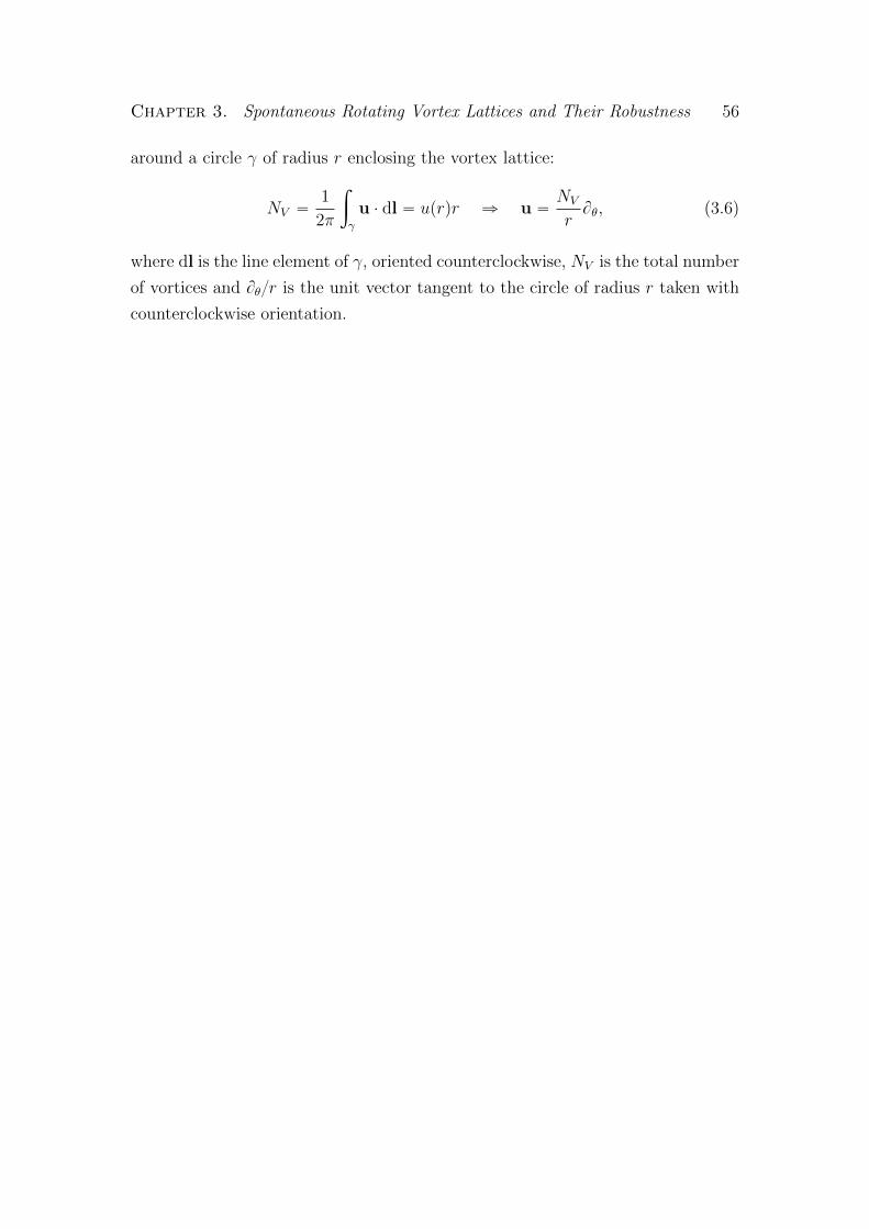
Chapter 3. Spontaneous Rotating Vortex Lattices and Their Robustness 56
around a circle γ of radius r enclosing the vortex lattice:
NV “1
2π
ż
γ
u ¨ dl “ uprqr ñ u “NV
rBθ, (3.6)
where dl is the line element of γ, oriented counterclockwise, NV is the total number
of vortices and Bθr is the unit vector tangent to the circle of radius r taken with
counterclockwise orientation.
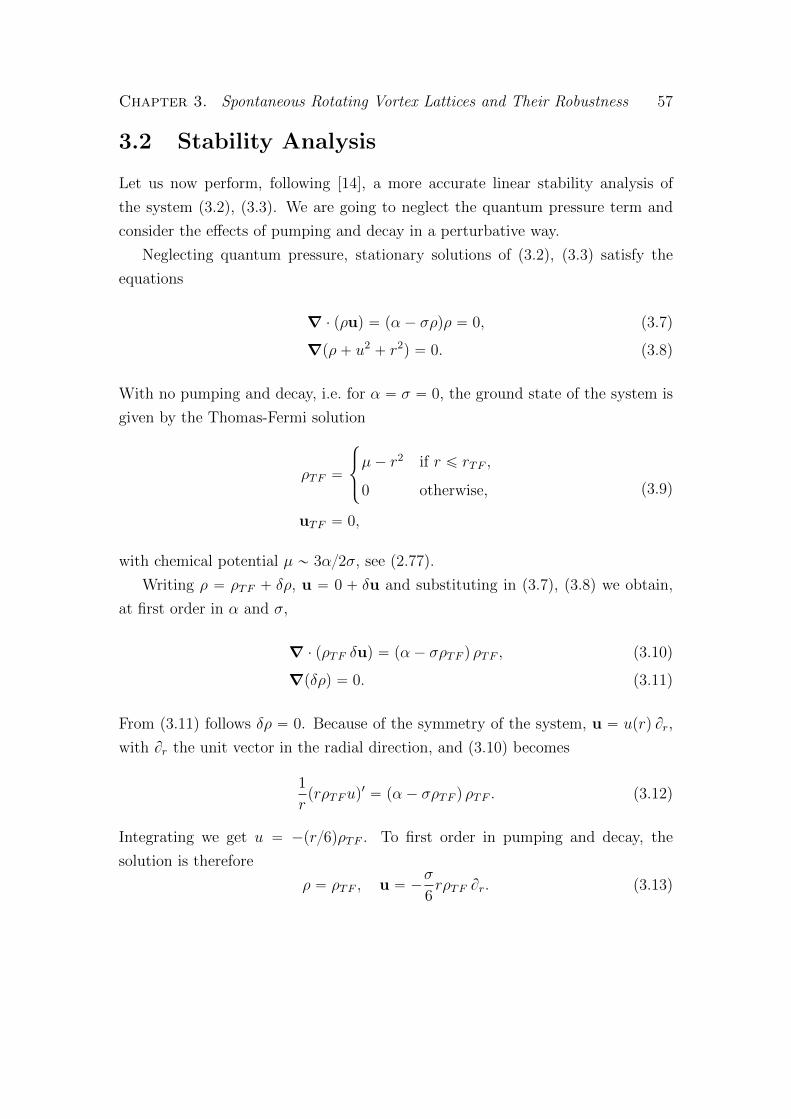
Chapter 3. Spontaneous Rotating Vortex Lattices and Their Robustness 57
3.2 Stability Analysis
Let us now perform, following [14], a more accurate linear stability analysis of
the system (3.2), (3.3). We are going to neglect the quantum pressure term and
consider the effects of pumping and decay in a perturbative way.
Neglecting quantum pressure, stationary solutions of (3.2), (3.3) satisfy the
equations
∇ ¨ pρuq “ pα ´ σρqρ “ 0, (3.7)
∇pρ` u2` r2
q “ 0. (3.8)
With no pumping and decay, i.e. for α “ σ “ 0, the ground state of the system is
given by the Thomas-Fermi solution
ρTF “
$
&
%
µ´ r2 if r ď rTF ,
0 otherwise,
uTF “ 0,
(3.9)
with chemical potential µ „ 3α2σ, see (2.77).
Writing ρ “ ρTF ` δρ, u “ 0 ` δu and substituting in (3.7), (3.8) we obtain,
at first order in α and σ,
∇ ¨ pρTF δuq “ pα ´ σρTF q ρTF , (3.10)
∇pδρq “ 0. (3.11)
From (3.11) follows δρ “ 0. Because of the symmetry of the system, u “ uprq Br,
with Br the unit vector in the radial direction, and (3.10) becomes
1
rprρTFuq
1“ pα ´ σρTF q ρTF . (3.12)
Integrating we get u “ ´pr6qρTF . To first order in pumping and decay, the
solution is therefore
ρ “ ρTF , u “ ´σ
6rρTF Br. (3.13)

Chapter 3. Spontaneous Rotating Vortex Lattices and Their Robustness 58
Consider now the perturbation, carrying angular momentum s,
ρprq Ñ ρprq ` hprq eipsθ´ωtq, uprq Ñ uprq ` vprq eipsθ´ωtq. (3.14)
Substituting in (3.2), (3.3), neglecting quantum pressure1 and writing ω “ ω0`δω
we have, at first order in v and h,
i pω0 ` δωq h eipsθ´ωtq “∇ ¨ pρv eipsθ´ωtq ` hu eipsθ´ωtqq ` p2σρ´ αqh eipsθ´ωtq,
i pω0 ` δωq v eipsθ´ωtq “∇ˆ
h
2eipsθ´ωtq ` u ¨ v eipsθ´ωtq
˙
.
(3.15)
Switching to polar coordinates pr, θq and using (2.68) we have
i pω0 ` δωq h “1
r
d
drprρ vrq `
isρ vθr
` p2σρ´ αqh`1
r
d
drpru hq,
i pω0 ` δωq vr “1
2
dh
dr`
d
drpu vrq,
i pω0 ` δωq vθ “is
2rh`
isu
rvr.
(3.16)
At zeroth order in pumping and decay, ρ “ ρTF , u “ α “ σ “ 0, hence
iω0 h “1
r
d
drprρTF vrq `
isρTFr
vθ, (3.17)
iω0 vr “1
2
dh
dr, (3.18)
iω0 vθ “is
2rh. (3.19)
Substituting (3.18) and (3.19) in (3.17) we get the hypergeometric ODE
1
2r
d
dr
ˆ
rρTFdh
dr
˙
´s2ρTF
2r2h “ ´ω2
0h. (3.20)
1The treatment given here does not apply to arbitrary perturbations but only to those havinga length scale such that neglecting quantum pressure is justified. However a more completetreatment would only be needed if without quantum pressure the system had no instabilities,and that is not the case.

Chapter 3. Spontaneous Rotating Vortex Lattices and Their Robustness 59
The general solution of (3.20) is
h “ C1
´
´µ
r2
¯s2
2F 1
ˆ
a1, b1; 1´ s;r2
µ
˙
` C2
ˆ
´r2
µ
˙s2
2F 1
ˆ
a2, b2; 1` s;r2
µ
˙
,
(3.21)
where C1, C2 are arbitrary constants, 2F1pa, b; c; zq is the hypergeometric function
2F1 “
8ÿ
k“0
paqkpbqkpcqk
zk
k!, (3.22)
with
pqqk “
$
&
%
1 if n “ 0,
qpq ` 1q ¨ ¨ ¨ pq ` n` 1q if k ą 0,(3.23)
and
a1 “1
2
ˆ
1´ s´b
1` s2 ` 2ω20
˙
, b1 “1
2
ˆ
1´ s`b
1` s2 ` 2ω20
˙
,
a2 “1
2
ˆ
1` s´b
1` s2 ` 2ω20
˙
, b2 “1
2
ˆ
1` s`b
1` s2 ` 2ω20
˙
.
(3.24)
Since equation (3.21) is invariant under the transformation sÑ ´s we can without
any loss of generality consider the case s ą 0. Then in order for h to be regular
at r “ 0 we need to take C1 “ 0. In order for 2F1pa, b; c; r2µq to be bounded as
r2 Ñ µ we need the series (3.22) to terminate after a finite number of terms. This
is possible if a2 “ ´n, with n a positive integer, which implies
ω0,ns “a
sp1` 2nq ` 2npn` 1q. (3.25)
Therefore (3.20) has the eigenfunctions
hRnsprq “ rs 2F1p´n, s` 1;n` s` 1; r2q, (3.26)
with eigenvalues (3.25). Note that hRns is real, therefore hR˚ns “ hRns. To this order,
the velocity (right) eigenfunctions vRr,ns, vRθ,ns are related to hRns by (3.18) and (3.19).
Let us now see how non-zero values of α and σ affect the eigenvalues (3.25).

Chapter 3. Spontaneous Rotating Vortex Lattices and Their Robustness 60
Rewrite (3.16) in the form
ipL` αδLqpψRns ` δψRnsq “ pω0,ns ` δωnsqpψRns ` δψ
Rnsq, (3.27)
where the operators iL and iδL are
iL “ i
¨
˚
˝
0 ´1r
ddrprρTF ´ is
rρTF
´12
ddr
0 0
´ is2r
0 0
˛
‹
‚
, (3.28)
iα δL “ i
¨
˚
˝
´2σρTF ` α ´1r
ddrpru 0 0
0 ´ ddrpu 0
0 ´ isru 0
˛
‹
‚
, (3.29)
and ψRns “ phRns, v
Rr,ns, v
Rθ,nsq
T denotes a right eigenfunction of iL. At first order in
the perturbation,
δωns ψRns “ piL´ ω0,nsq δψ
Rns ` iα δLψRns. (3.30)
If iL were self-adjoint, we could find δωns as in standard perturbation theory,
multiplying (3.30) by pψRnsq˚, integrating over the whole domain, and making use
of the identityż
d2x pψRnsq˚iL “ ω0,ns
ż
d2x pψRnsq˚. (3.31)
However, since iL is not self-adjoint, left eigenfunctions are generally not the

Chapter 3. Spontaneous Rotating Vortex Lattices and Their Robustness 61
complex conjugate of right eigenfunctions.2 Instead we have
δωns
ż
d2xψLns ψRns “ iα
ż
d2xψLnsδLψRns `ż
d2xψLns piL´ ω0,nsq δψRns, (3.32)
where the integral is over the disk of radius rTF “?µ,
ż
d2x “
ż
?µ
0
r dr
ż 2π
0
dθ. (3.33)
In order to solve for δωns, we need to find the left eigenfunctions. Since left
and right eigenfunctions have the same eigenvalues, we need to impose that, for
any ψ,
I “
ż
d2xψLns iLψ “ ω0,ns
ż
d2xψLnsψ (3.34)
so that the last term in (3.32) vanishes. Using (3.28) and writing ψ “ ph, vr, vθqT ,
2Left and right eigenvalues are always equal. Suppose vL is a right eigenvector (columnvector) of a linear operator A with eigenvalue λL and vR a right eigenvector (row vector) witheigenvalue λR,
vLA “ λLvL, AvR “ λRvR.
Taking the adjoint of the first equation we have
A:`
vL˘:“
`
λL˘˚ `
vL˘:.
Left eigenvalues of A therefore satisfy the equation
det´
A: ´`
λL˘˚I¯
“`
det`
A´ λLI˘˘˚
“ 0,
which has the same solutions as the equation for the right eigenvalues
det`
A´ λRI˘
“ 0.
Therefore λL “ λR “ λ and
A:`
vL˘:“ λ
`
vL˘:,
AvR “ λvR.
If A “ A: then we also have vL “ pvRq:, but this is not generally true.

Chapter 3. Spontaneous Rotating Vortex Lattices and Their Robustness 62
ψLns “ phLns, v
Lr,ns, v
Lθ,nsq we have
I “
ż
d2x
„
hLns
ˆ
´i
r
d
drprρTF vrq `
s
rρTF vθ
˙
´ vLr,nsi
2
dh
dr` vLθ,ns
s
2rh
. (3.35)
Using (3.17), (3.18), (3.19), one can verify that (3.34) is satisfied provided that
hLns “`
hRns˘˚“ hRns, vLr,ns “ 2ρTF
`
vRr,ns˘˚, vLθ,ns “ 2ρTF
`
vRθ,ns˘˚. (3.36)
The shift in frequency δωns is then, up to first order in α and σ,
δωns “ iα
ş
d2xψLns δLψRnsş
d2xψLns ψRns
. (3.37)
Let us evaluate (3.37) explicitly. To first order in pumping and decay, ρ and u
are given by (3.13). Therefore the denominator of (3.37) is
ż
d2xψLnsψRns “
ż
d2x´
|hRns|2` 2ρTF
`
|vRr,ns|2` |vRθ,ns|
2˘
¯
“
ż
d2x
˜
`
hRns˘2`
ρTF2ω2
0,ns
ˆ
dhRnsdr
˙2
`s2ρTF
`
hRns˘2
2ω20,nsr
2
¸
,
(3.38)
having used (3.18), (3.19). Since pρTF rqp?µq “ pρTF rqp0q “ 0, integrating the
second term by part,
ż
d2xψLnsψRns
“ 2π
ż
?µ
0
ˆ
hRns ´1
2rω20,ns
d
dr
ˆ
ρTF rdhRnsdr
˙
´ρTF
2ω20,ns
d2hRnsdr2
`s2ρTFh
2ω20,nsr
2
˙
rhRns
“ 2
ż
d2x`
hRns˘2,
(3.39)
having used (3.20) for the last equality.

Chapter 3. Spontaneous Rotating Vortex Lattices and Their Robustness 63
The numerator of (3.37) is, using (3.29), (3.18), (3.19),
iα
ż
d2xψLnsδLψRns “
“ 2πi
ż
dr r
ˆ
pα ´ 2σρTF q`
hRns˘2´
hRnsr
d`
r u hRns˘
dr´
ρTF2ω2
0,ns
dhRnsdr
d
dr
ˆ
udhRnsdr
˙
´s2u ρTF2ω2
0,ns r2hRns
dhRnsdr
˙
.
(3.40)
Since up0q “ up?µq “ 0, integrating by parts the second and third terms we obtain
iα
ż
d2xψLns δLψRns
“
ż
d2x”
pα ´ 2σρTF q`
hRns˘2
` udhRnsdr
ˆ
hRns `1
2ω20,ns r
d
dr
ˆ
ρTF rdhRnsdr
˙
´s2ρTF
2ω20,ns r
2hRns
˙
ı
“ i
ż
d2x pα ´ 2σρTF q`
hRns˘2,
(3.41)
having used (3.20). Therefore
δωns “i
2
ş
d2x pα ´ 2σρTF q`
hRns˘2
ş
d2x phRnsq2 “
i
2
`
α ´ 2σµ` 2σ@
r2D˘
“iα
2
ˆ
3
µ
@
r2D
´ 2
˙
,
(3.42)
having used the relation µ “ 3αp2σq to eliminate σ and defined
@
r2D
“
ş
d2x r2`
hRns˘2
ş
d2x phRnsq2 . (3.43)
As we can see from equation (3.42), any mode that transfers density to large radius,
and therefore has a large expectation value of r2, has a positive imaginary part
and therefore destabilises the system.

Chapter 3. Spontaneous Rotating Vortex Lattices and Their Robustness 64
In order to evaluate xr2y multiply equation (3.20) by r2ρTF dhRnsdr obtaining
1
2
d
dr
ˆ
rρTFdhRnsdr
˙2
“
ˆ
s2ρ2TF
2´ ω2
0,nsr2ρTF
˙
d`
hRns˘2
dr. (3.44)
Since pρTF rqp0q “ pρTF rqp?µq “ 0, hRnsp0q “ 0, integrating by parts,
0 “1
2
ż
?µ
0
drd
dr
ˆ
ρTF rdhRnsdr
˙2
“
ż
?µ
0
dr
ˆ
s2ρ2TF
2´ ω2
0,ns ρTF r2
˙
d`
hRns˘2
dr
“ ´
ż
?µ
0
drd
dr
ˆ
s2ρ2TF
2´ ω2
0,ns ρTF r2
˙
`
hRns˘2.
(3.45)
It follows
ps2` 2ω2
0,nsq
ż
?µ
0
r dr r2phRnsq
2“ µpω2
0,ns ` s2q
ż
?µ
0
r drphRnsq2, (3.46)
hence@
r2D
“ µs2 ` ω2
0,ns
s2 ` 2ω20,ns
, (3.47)
and
δωns “iα
2
ˆ
s2 ´ ω20,ns
s2 ` 2ω20,ns
˙
“iα
2
ˆ
s2 ´ sp1` 2nq ´ 2npn` 1q
s2 ` 2sp1` 2nq ` 4npn` 1q
˙
. (3.48)
For any fixed n, there is always an s, e.g. s " n, such that (3.48) has a positive
imaginary part. A similar analysis shows that the instability is still present if the
relaxation term η in (2.32) has a non-zero value [14].

Chapter 3. Spontaneous Rotating Vortex Lattices and Their Robustness 65
3.3 Robustness
In this section, based on [14], three different kinds of perturbations are considered:
non-circular geometry of the trap, disorder and changes to the modelling equation.
3.3.1 Elliptical Deformations of the Trap
Figure 3.2: Density (colour map) and superfluid streamlines (arrows) for differentsizes of the pumping spot, whose boundary is denoted by a red ellipse. Left(δ “ 0.9, R “ 7): the surface instability leads to a spontaneously formed latticewith vortices moving along elliptical trajectories. Right (δ “ 0.9, R “ 4): if thepumping spot is smaller than rTF the instability does not appear.
Consider equation (3.1) with the circular trap replaced by an elliptical one,
r2Ñ
x2
δ2` δ2y2. (3.49)
The parameter δ, is related to the eccentricity ε of the ellipse by the relation
ε “a
1´ 1δ4. Pumping is constant inside the ellipse x2δ2 ` δ2y2 “ R2. Since
we are considering pumping at twice threshold, the value of α outside the pumping

Chapter 3. Spontaneous Rotating Vortex Lattices and Their Robustness 66
spot is the same as the one inside but with the opposite sign: with respect to (3.1),
αÑ α
„
Θ
ˆ
R2´
ˆ
x2
δ2` δ2y2
˙˙
´Θ
ˆˆ
x2
δ2` δ2y2
˙
´R2
˙
, (3.50)
where Θ is the Heaviside function.
Figure 3.3: The averaged orbits of three vortices (green, magenta and orangeellipses) superimposed over the density profile of the condensate at the momentwhen the vortex tracing has been started. The initial positions of the tracedvortices are denoted by green, magenta and orange crosses. The red, solid ellipsemarks the boundary of the pumping spot.
As in the circular case, the surface instability appears only if R ą rTF , see
figure 3.2. We have investigated the effects of a varying δ while keeping R “ 7
fixed. For not too eccentric traps, a rotating vortex lattice with vortices moving
along elliptical orbits still forms, as shown in figure 3.3.
The vortices orbits have been found by tracing the positions of individual vor-
tices from a time step to the following one and averaging over several revolutions.
The position of a vortex at time t` δt has been found by searching for a minimum
of the density taking the position of the vortex at time t as the starting point of

Chapter 3. Spontaneous Rotating Vortex Lattices and Their Robustness 67
Figure 3.4: Left (δ “ 0.85): the regular vortex lattice is broken up, with some vor-tices still moving along regular elliptic orbits. Right (δ “ 0.80): as δ decreases, therotating lattice gives way to a fragmented state with vortices continually enteringand leaving the cloud.
the search. Because vortices have a definite sense of rotation, the motion is not
symmetric around the major axis, and the resulting lattice is tilted with respect
to the trap.
For a sufficiently eccentric geometry, a steady array of vortices fails to form.
There is a critical δ „ 0.85 for which some vortices still move on elliptical orbits,
see figure 3.4, left panel. At δ “ 0.8, the behaviour is entirely chaotic, with
vortices continually entering and leaving the cloud, see figure 3.4, right panel,
causing fragmentation of the condensate.
In the limit of extreme eccentricity, the condensate tries to establish a density
profile of approximately uniform width along the trap major axis, leading to a less
fragmented condensate at δ À 0.2, see figure 3.5. Instability towards the entrance
of vortices is still present: vortices entering and leaving the cloud cause transverse
oscillations. As illustrated in the bottom right panel of figure 3.5, vortices of
opposite signs may be present. The distribution of vortices of different sign may

Chapter 3. Spontaneous Rotating Vortex Lattices and Their Robustness 68
Figure 3.5: Top left (δ “ 0.25): in a highly eccentric trap, the condensate triesto establish a profile of approximately uniform width along the trap major axis— the vertical direction in the figure. Instability towards the entrance of vorticesleads to transverse oscillations. Note that the vertical axis has been rescaled inorder to accommodate the extreme eccentricity. Top right (δ “ 0.1): extremeeccentricity suppresses fragmentation of the cloud. Transverse oscillations developat the midpoint. Bottom left (δ “ 0.1): spontaneously entering vortices causean effective pressure gradient, pushing the region of perturbations towards oneend of the trap. The final position of the perturbation is shown. Bottom right(δ “ 0.1): vortices of both signs are present in the perturbed region. Arrowsindicate circulation.

Chapter 3. Spontaneous Rotating Vortex Lattices and Their Robustness 69
lead to a net effective pressure in the condensate pushing the perturbation along
the length of the condensate until the pressure gradient disappears. This effect
is illustrated in the bottom left panel of figure 3.5 which shows the final position
of the region of perturbations. Note that a true stationary state is not obtained:
oscillations are still present.
3.3.2 Effects of Disorder on the Rotating State
In the samples used in experiments disorder is always present [79]. We take this
into account by including a disorder term Vdispxq in the potential Vextpxq:
V pxq Ñ V pxq ` Vdispxq. (3.51)
This disorder potential is modelled as a Gaussian random field with real-space
correlation function
xVdispxqVdispx1qy “ V 2
0 exp
ˆ
´|x´ x 1|2
2ξ2
˙
, (3.52)
where the amplitude V0 measures the disorder strength, and ξ its correlation length.
The Gaussian random field Vdispxq can be constructed by taking the Fourier
sum
Vdispxq “1
2
ÿ
i,j
aij exp`
i pki x` kj y ` φijq˘
, (3.53)
with k´i “ ´ki, k´j “ ´kj, φ´i´j “ ´φij. The phases φij are random numbers
in the interval r0, 2πq. The amplitudes aij “ a´i´j are sampled from a Gaussian
distribution with zero mean and standard deviation
sij “ v0 exp“
´l2c`
k2i ` k
2j
˘‰
. (3.54)
The relation between the parameters v0 and lc, defined for computational con-
venience, and the physical disorder strength V0 and correlation length ξ can be

Chapter 3. Spontaneous Rotating Vortex Lattices and Their Robustness 70
found by noting that
xaijauv eipφij`φuvqy “ δiuδjv xa2ije
2φijy ` δi´uδj´v xa2ijy “ δi´uδj´v s
2ij
“ δi´uδj´v v20 exp
`
´ 2l2c pk2x ` k
2yq˘
.(3.55)
It follows
xVdispxqVdispx1qy “
1
4
ÿ
ij
ÿ
uv
xaijauveipφij`φuvqyeipkix`kjy`kux
1`kvy1q
“1
4
ÿ
ij
s2ije
ipkipx´x1q`kjpy´y
1qq
»1
4p∆kq2
ż
R2
v20e´2l2cpk2x`k2yqeipkipx´x
1q`kjpy´y1qqdkxdky
“v2
0
4p∆kq2π
2l2cexp
”
´px´ x1q2
8l2c
ı
,
(3.56)
where ∆k is the numerical Fourier mode spacing and we have replaced k-space
sums by integrals. Comparing (3.52) with (3.56) we have
ξ “ 2lc, V0 “v0
a
π2
2lc∆k. (3.57)
Varying V0 and ξ we find that the formation of a vortex lattice is sensitive to
the disorder strength, with the lattice being destroyed for V0 ą Vcrit » 6.5. For
the stress trap of [10] our estimate translates in a critical disorder Vcrit » 0.4 meV,
subject to uncertainties in the estimates of experimental quantities as well as to
effects not accounted for in our model, such as relaxation mechanisms. When the
disorder strength exceeds Vcrit the behaviour is chaotic and no stationary state
forms. However, the critical amount of disorder is only weakly dependent on the
disorder correlation length ξ, as illustrated by the nearly horizontal border in the
pV0, ξq-diagram of figure 3.6.

Chapter 3. Spontaneous Rotating Vortex Lattices and Their Robustness 71
Figure 3.6: The figure is based on a particular realisation of the random potentialVdis, different realisations giving very similar results. Top: a rotating vortex latticeforms also in the presence of weak disorder (a), but is destroyed by a disorderstronger than Vcrit, leading to a chaotic state (b). Bottom: the boundary betweenvortex-lattice and chaotic regimes in the pV0, ξq parameter space. The choices ofpV0, ξq leading to the states (a) and (b) are indicated in the diagram. The vortexlattice is strongly sensitive to the amount of disorder, whereas the correlationlength is only of marginal importance.
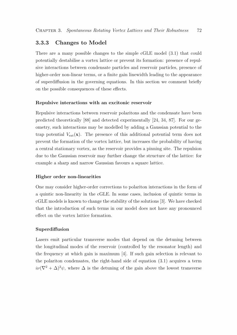
Chapter 3. Spontaneous Rotating Vortex Lattices and Their Robustness 72
3.3.3 Changes to Model
There are a many possible changes to the simple cGLE model (3.1) that could
potentially destabilise a vortex lattice or prevent its formation: presence of repul-
sive interactions between condensate particles and reservoir particles, presence of
higher-order non-linear terms, or a finite gain linewidth leading to the appearance
of superdiffusion in the governing equations. In this section we comment briefly
on the possible consequences of these effects.
Repulsive interactions with an excitonic reservoir
Repulsive interactions between reservoir polaritons and the condensate have been
predicted theoretically [88] and detected experimentally [24, 34, 87]. For our ge-
ometry, such interactions may be modelled by adding a Gaussian potential to the
trap potential Vextpxq. The presence of this additional potential term does not
prevent the formation of the vortex lattice, but increases the probability of having
a central stationary vortex, as the reservoir provides a pinning site. The repulsion
due to the Gaussian reservoir may further change the structure of the lattice: for
example a sharp and narrow Gaussian favours a square lattice.
Higher order non-linearities
One may consider higher-order corrections to polariton interactions in the form of
a quintic non-linearity in the cGLE. In some cases, inclusion of quintic terms in
cGLE models is known to change the stability of the solutions [3]. We have checked
that the introduction of such terms in our model does not have any pronounced
effect on the vortex lattice formation.
Superdiffusion
Lasers emit particular transverse modes that depend on the detuning between
the longitudinal modes of the reservoir (controlled by the resonator length) and
the frequency at which gain is maximum [4]. If such gain selection is relevant to
the polariton condensates, the right-hand side of equation (3.1) acquires a term
iνp∇2 ` ∆q2ψ, where ∆ is the detuning of the gain above the lowest transverse

Chapter 3. Spontaneous Rotating Vortex Lattices and Their Robustness 73
mode. Such mechanisms have not been extensively discussed in the context of
polariton condensation, but the essence appears for example in [30]. Our numerical
simulations show that although the lattice survives for small values of ν, the rings
of vortices are shifted to the boundary of the condensate. The lattice disappears
for ν ą 0.1.

Chapter 4
Polariton Gyroscope
Polariton condensates allow for a high degree of experimental control. For example,
it is possible to engineer any external potential and to vary pumping in space and
time. In response to slight changes in the environment, e.g. when flows exceed some
critical velocity, when fluxes interact, when pumping powers exceed a threshold
for pattern forming instabilities, polariton condensates nucleate quantised vortices.
Therefore, one could prepare the system in a state slightly below the criticality
for vortex formation so that a tiny external perturbation will take it over the
criticality, leading to a macroscopic and easily detectable response.
This mechanism can be exploited for the construction of a polariton gyroscope.
Superfluid helium gyroscopes have already been shown to provide sensitive means
for detecting absolute rotations [7, 71], but require very low temperatures for
operation. Compared to superfluid helium gyroscopes, polariton-based ones offer
the advantage of potentially operating at room temperatures and of allowing easy
experimental control of many of their properties.
Section 4.1 introduces the apparatus. Section 4.2 discusses the role of the
external potential in controlling the vortex formation mechanism in a simplified
1-dimensional configuration, where analytical estimates for the condensate wave
function can be made. Section 4.3 illustrates the 2-dimensional model and presents
the results of numerical simulations.
4.1 The Apparatus
The spectrum of low-energy excitations of a polariton condensate is purely imagi-
nary for low momentum, see appendix A.1, therefore a direct application of Lan-
dau’s criterion for superfluidity would give a vanishing critical velocity. However
theoretical studies taking into account the non-equilibrium properties of the system
and results of recent experiments both indicate that polariton condensates share
with superfluids the ability of flowing with very low friction at small velocities
[1, 89].
74

Chapter 4. Polariton Gyroscope 75
The basic setup of our gyroscope is similar to that proposed for superfluid
helium gyroscopes [71]: an annulus filled with superfluid having a partition with
a small opening, see figure 4.1. We denote by R1 the inner radius of the annulus
and by R2 the outer radius. We assume that R2 ´R1 ! R1, and denote by R the
mean radius pR2 `R1q2.
If an annulus filled with polariton condensate is rotated counterclockwise about
a central axis with angular velocity Ω “ Ω Bz, the condensate experiences negligible
friction with boundaries and remains motionless. If a partition is inserted into the
annulus, a rotation of the apparatus sets the condensate in motion with a speed
given in first approximation by the rigid body value ΩR [71]. If the partition has a
small opening (weak link) of width δ, the flow is not significantly affected far from
it but a flow in the direction opposite to that of rotation is generated through the
opening. To leading order, the velocity across the aperture is given by U “ ΩR2δ,
with corrections due to the non-zero compressibility of a polariton fluid. Typical
values of R and δ for existing apparatuses are R „ 0.1 m, δ „100 nm, providing
an amplification factor Rδ „ 106.
If U exceeds some critical value Uc, vortices are nucleated and can be detected
as phase slips. In the case of superfluid 4He Uc „ 50 m/s. However for polariton
condensates Uc is of the order of equilibrium sound speed [89], given, for typical
values of the condensate density, by 1 – 5 µm/ps = 1 – 5 ¨106 m/s. Therefore
the high critical velocity of polariton condensates could limit the sensitivity of the
apparatus.
However, and here is the novelty of the approach that we propose, the veloc-
ities needed to start vortex nucleation can be greatly reduced by using pumping
strength as a control parameter and by engineering an external potential through
the weak link, see figure 4.1. Such a potential, which accelerates the condensate
and allows to control the vortex nucleation process, can be prepared either by us-
ing a combination of etching [28, 49, 9] and stress induced traps [10], or by directly
defining blue-shifted trap potentials via spatial light modulators [85].
Even in the absence of any externally applied flow, velocity fluxes connecting
regions where the density is low (at the potential peak) to regions where the den-
sity is high (at the potential dip) will be generated; in between them there will
be a point where the condensate speed takes its maximum value. Close to such a

Chapter 4. Polariton Gyroscope 76
Ω
U
PumpingU
Vext
Figure 4.1: Schematic of the apparatus: an annulus filled with polariton conden-sate having a partition with a weak link. If the flow across the link is high enough,vortices are generated. The inset shows a cross section of the external potentialthrough the weak link.
point, the density has a local minimum (Bernoulli effect). A slight change of some
experimentally accessible parameter, e.g. an increase of the potential strength, or
a decrease of the pumping intensity, will further lower the density. If the pertur-
bation is large enough, the density minimum will reach zero and a vortex pair will
be emitted, as we illustrate in section 4.3.
The procedure for measuring rotations follows: having prepared a potential
such that the system is in a slightly subcritical configuration for the range of rota-
tion speeds that one intends to measure, the pumping strength is varied, recording
the moment at which vortices start being nucleated. From this, once the appara-
tus has been calibrated, one can deduce the back-flow through the weak link and,
therefore, the rotational velocity.
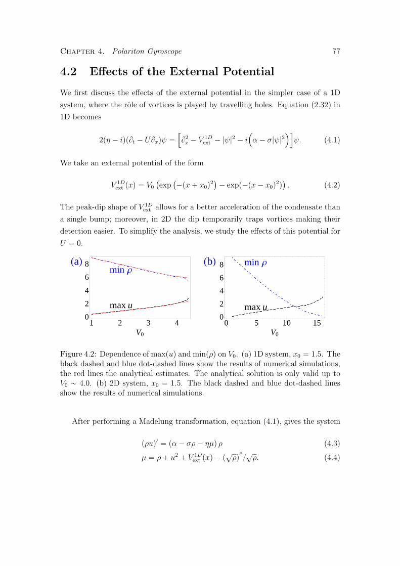
Chapter 4. Polariton Gyroscope 77
4.2 Effects of the External Potential
We first discuss the effects of the external potential in the simpler case of a 1D
system, where the role of vortices is played by travelling holes. Equation (2.32) in
1D becomes
2pη ´ iqpBt ´ UBxqψ “”
B2x ´ V
1Dext ´ |ψ|
2´ i
´
α ´ σ|ψ|2¯ı
ψ. (4.1)
We take an external potential of the form
V 1Dext pxq “ V0
`
exp`
´px` x0q2˘
´ expp´px´ x0q2q˘
. (4.2)
The peak-dip shape of V 1Dext allows for a better acceleration of the condensate than
a single bump; moreover, in 2D the dip temporarily traps vortices making their
detection easier. To simplify the analysis, we study the effects of this potential for
U “ 0.
min Ρ
max u
1 2 3 40
2
4
6
8
V0
min Ρ
max u
0 5 10 150
2
4
6
8
V0
HaL HbL
Figure 4.2: Dependence of max(u) and min(ρ) on V0. (a) 1D system, x0 “ 1.5. Theblack dashed and blue dot-dashed lines show the results of numerical simulations,the red lines the analytical estimates. The analytical solution is only valid up toV0 „ 4.0. (b) 2D system, x0 “ 1.5. The black dashed and blue dot-dashed linesshow the results of numerical simulations.
After performing a Madelung transformation, equation (4.1), gives the system
pρuq1 “ pα ´ σρ´ ηµq ρ (4.3)
µ “ ρ` u2` V 1D
ext pxq ´ p?ρq2
?ρ. (4.4)

Chapter 4. Polariton Gyroscope 78
The speed u takes its maximum at some point between the maximum, close to
´x0 and and the minimum, close to x0, of Vext. As follows from (4.4), which is a
generalised Bernoulli equation, in proximity of the speed maximum the density has
a local minimum. The numerical results displayed in figure 4.2 show that maxpuq
V0=1
V0=2
V0=3
V0=4
-4 -2 0 2 4-0.5
0.0
0.5
1.0
1.5
2.0
x
u
-4 -2 0 2 4
6789
101112
xΡ
HaL HbL
Figure 4.3: (a) Numerical (black dashed lines) and analytical estimates (red solidlines) of the condensate velocity as V0 is increased from 1 to 4. (b) Numericalsolutions for ρ with V0 “ 1.4, 2.0, 2.6, 3.2, 3.8, 4.4. Higher values of V0 correspondto lower values of min(ρ). In both figures x0 “ 1.5.
is an increasing function of V0 and min(ρ) a decreasing one.
This behaviour can be verified analytically by deriving an approximate solution
of the system (4.3), (4.4). For very small V0 it is natural to expect a dip-peak
density profile, that is inverted with respect to that of the potential; however,
for higher values of V0, there will be an additional minimum due to the Bernoulli
effect. Therefore we take an ansatz for the density of the form
ρ “α
σ ` η`B expp´bpx´ x3q
2q ` C expp´cpx´ x1q
2q ´Q expp´qpx´ x2q
2q,
(4.5)
where b, B, c, C, q,Q, x1, x2, x3 are free parameters. Substituting in (4.3) and inte-

Chapter 4. Polariton Gyroscope 79
Figure 4.4: Travelling holes, identified by the localised low-density blue region,form around x “ 0, and travel up to x „ 1.5. The process repeats periodically intime. (V0 “ 4.8, x0 “ 1.5, α “ 4).
grating we have
ρu “
?πασ
2pσ ` ηq
«
Q?q
erf p?qx3q ´
B?berfp?bx1q ´
C?cerf
`?cx2
˘
ff
´
c
π
2
σ
2
«
B2
?berfp?
2bx1q `C2
?cerfp?
2cx2q `Q2
?q
erfpa
2qx3q
ff
`?πσ
«
´ EpB,C, b, c, x1, x2q ` EpB,Q, b, q, x1, x3q
` EpC,Q, c, q, x2, x3q
ff
,
(4.6)
where xi ” x´ xi, xij ” xi ´ xj and
EpB,C, b, c, xi, xjq“BC?b` c
exp
ˆ
´b c x2
ij
b` c
˙
erf
ˆ
bxi ` cxj?b` c
˙
. (4.7)
Let Vextpxq be the potential obtained substituting ρ and u from (4.5) and (4.6)

Chapter 4. Polariton Gyroscope 80
in (4.4) and which contains the unknown parameters B,C,Q, b, c, q, x1, x2, x3. The
values of these parameters can be fixed by requiring Vextpxq to fit the original
potential V 1Dext pxq. A comparison of the analytical and numerical solutions for u is
shown in panel (a) of figure 4.3, while numerical solutions for ρ corresponding to
various values of V0 are shown in panel (b).
The dependence of max(u) and min(ρ) on V0 is mostly linear up to V0 “ 4,
see figure 4.2 panel (a). However, for V0 ą Vc „ 4.4, a deviation from the linear
regime quickly leads to the loss of stability of the stationary solutions. The time
dependent solutions found for V0 ą 4.4 are characterised by the periodic emission
of travelling holes [57], which travel for a short time before dissipating, see figure
4.4. As a hole is emitted, the density vanishes in correspondence of the point of
emission.
As we can see, varying an experimentally tunable parameter, in this case the
strength of the potential, leads to an easily detectable response of the system, in
this case the emission of travelling holes. As we shall see, similar mechanisms
operate in 2D.

Chapter 4. Polariton Gyroscope 81
4.3 The Model in 2D
In two dimensions we have the equation
Figure 4.5: Real space plots of the zero level of real (black continuous line) andimaginary (grey dashed line) part of ψ superimposed over the contour plot of ρ.Regions of higher density are in warmer colours. (a) (α “ 4, V0 “ 16.8, x0 “ 1.5,U “ 0): a slightly subcritical configuration. (b) (α “ 4, V0 “ 16.8, x0 “ 1.5,U “ 0.2): a slightly supercritical configuration at the moment of vortex pairformation. A red arrow shows the direction of the flow; a red dot marks the pointwhere the vortex pair is being generated.
2pη ´ iq pBt `U ¨∇qψ “”
∇2´ V 2D
ext ´ |ψ|2´ i
´
α ´ σ|ψ|2¯ı
ψ, (4.8)
where U „ ΩR is the bulk speed of the condensate, and
V 2Dext px, yq “ V0
`
expp´ppx` x0q2` y2
qq ´ expp´ppx´ x0q2` y2
qq˘
. (4.9)
The dependence of max(u) and min(ρ) on V0 is similar to the one we observed
in the 1-dimensional case, see figure 4.2 panel (b). When V0 exceeds some critical
value, stationary solutions again become unstable. In two dimensions the outcome
of this instability is the nucleation of vortex pairs. There is, however, one notable

Chapter 4. Polariton Gyroscope 82
difference with the 1D case: while in the latter the emission of travelling holes sets
in at a finite value of minpρq, in 2D there are stationary solutions all the way down
to min(ρ)“ 0, see the right panel of figure 4.2.
Figure 4.6: The 3D plots show the density of the condensate, with the externalpotential superimposed in yellow. The 2D contour plots give the projection of thedensity values on the x-y plane, with regions of higher density in warmer colours.The direction of the flow is from the left to the right. (a) (V0 “ 14, x0 “ 1.5, α “ 4,U “ 0.4): an supercritical state. A vortex pair has been temporarily trapped bythe dip in the potential. (b) (V0 “ 14, x0 “ 1.5, α “ 4, U “ 0): a subcriticalstationary solution.
If the system is close enough to criticality, vortex nucleation can be initiated
also by a small increase of the external velocity U or by a decrease of the pumping

Chapter 4. Polariton Gyroscope 83
strength α. An example of the process is illustrated in figure 4.5, where the onset
of vortex nucleation is caused by an increase in U . Representatives of supercritical
and subcritical states are shown in figure 4.6.
Vortex nucleation
No vortices
3. 3.5 4. 4.5
0.
0.2
0.4
0.6
Α
M
4.00 4.010.1
0.8
10-3
Figure 4.7: The main plot shows part of the boundary between supercritical andsubcritical regions of phase space with respect to the parameters M “ UUc, withUc the equilibrium sound speed, and α for V0 “ 14, x0 “ 1.5. The inset has beenobtained with a different value of the potential strength, V0 “ 16.8, x0 “ 1.5 andgives an idea of the attainable resolution for small values of M .
In many experimental configurations, the most convenient control parameter
is the pumping strength α. Figure 4.7 shows the critical values of α which start
vortex nucleation for fixed V0 and different values of M “ UUc. The boundary
Upαq between subcritical and supercritical behaviour is, for M À 0.5, nearly linear,
hence the sensitivity of the apparatus scales linearly with α or, equivalently, with
the bulk density αpσ ` ηq of the condensate.
For appropriate choices of V0, in our numerical simulations the system showed
a clear transition between subcritical and supercritical states down to velocities

Chapter 4. Polariton Gyroscope 84
U „ 10´4Uc, with Uc “a
µm the equilibrium sound speed, corresponding to a
minimum detectable angular velocity of „ 10´4 Hz, close to the Earth angular
velocity of „ 7 ¨ 10´5 Hz. A proper discussion of the apparatus sensitivity, which
would require to consider the dependence of the critical speed Uc on the temper-
ature and on the geometry of the aperture and to account for noise sources, is
outside the scope of this work, whose aim is to illustrate the basic idea. Improv-
ing on the basic setup discussed here, e.g. by considering external potentials of a
shape leading to an even greater reduction of the critical velocity for vortex nucle-
ation, it should be possible to greatly enhance the apparatus sensitivity, possibly
matching that of superfluid helium gyroscopes, which, according to a conservative
estimate, can in principle detect angular velocities as small as „ 10´7 Hz [71], com-
parable with current-technology FOG devices, but at the advantage of potentially
operating at room temperature.

Chapter 5
Influence of the Pumping
Geometry on the Dynamics
Recent experiments have shown that polaritons injected at two spatially separated
pump spots organise themselves so to produce a system which behaves very simi-
larly to a 1-dimensional quantum harmonic oscillator [85]. Subsequent experiments
with polaritons injected at multiple pump spots have revealed the importance of
the number of pumps and of their distances in determining the dynamical be-
haviour of the system [26]. In fact, as the distance between pumps is varied, the
system shows a transition from a phase-locked but freely flowing regime to a fully
trapped state.
Section 5.1 recapitulates the results of [85]. Section 5.2 discusses the results
presented in [26]. I have contributed to the theoretical work leading to [26] and
performed all the numerical simulations.
5.1 A Quantum Harmonic Oscillator
Consider a system where polaritons are injected at two different pump spots. Be-
cause of the repulsive interactions between polaritons and reservoir excitons, the
polaritons at each spot will feel an effective potential of approximately Gaussian
shape, see figure 5.1, panel (a). Descending the respective potential hills, the two
condensates soon come into contact and lock in phase so that the resulting system
can be described by a single wave function.
The phase-locking mechanism can be understood by analysing the temporal
dynamics of the phases of the two condensates. Let ψ1 “?ρ1 exppi φ1q, ψ2 “
?ρ2 exppi φ2q be the condensates wave functions. It is convenient to factor out a
global phase χ by writing φ1 “ χ` φ2, φ2 “ χ´ φ2. Since we are interested in
the time evolution of φ1, φ2, we neglect spatial dynamics and consider the coupled
85

Chapter 5. Influence of the Pumping Geometry on the Dynamics 86
Figure 5.1: Image taken from [85]. (a) The experimental setup: two pump spotsof diameter 1 µm distant 20 µm from each other. The resulting potential (in red),combined with the effects of polariton-polariton interactions, produces quantumoscillator states, like the one shown at the top of the panel. (b) Energy spectrumalong the line connecting the two pump spots superimposed over the shape of theeffective potential. (c) Contour plots of the observed condensate density showingvarious harmonic oscillator modes. (d) Dependence of the energy on the quantumnumber. (e) Hermite-Gaussian fit of the n “ 5 state.
equations
2i Btψ1 “ rρ1 ` p1´ uqρ2 ` ipα ´ σρ1qsψ1 ` Jψ2, (5.1)
2i Btψ2 “ rρ2 ` p1´ uqρ1 ` ipα ´ σρ2qsψ2 ` Jψ1, (5.2)
where the term 1 ´ u, with u ă 1, represents the repulsive interactions between
the two condensates and J is the Josephson coupling constant. Multiplying (5.1)
by?ρ1 expp´ipχ`φ2qq, (5.2) by
?ρ2 expp´ipχ´φ2qq and taking the sum yields
i Btpρ1 ` ρ2q ´ 2pρ1 ` ρ2q 9χ´ pρ1 ´ ρ2q9φ
“ pρ1 ` ρ2q2´ 2uρ1ρ2 ` 2J
?ρ1ρ2 cosφ` i
“
x2pρ1 ` ρ2q ´ σpρ
21 ` ρ
22q‰
.(5.3)

Chapter 5. Influence of the Pumping Geometry on the Dynamics 87
Defining
R “ρ1 ` ρ2
2, z “
ρ1 ´ ρ2
2(5.4)
and separating real and imaginary part one obtains the equations
2R 9χ` z 9φ “ ´2R2` upR2
´ z2q ´ J
?R2 ´ z2 cosφ, (5.5)
9R “ αR ´ σpR2` z2
q. (5.6)
Similarly, multiplying (5.1) by?ρ1 expp´ipχ ` φ2qq, (5.2) by
?ρ2 expp´ipχ ´
φ2qq, taking the difference and separating real and imaginary part yields
9z “ zpα ´ 2σRq ´ J?R2 ´ z2 sinφ, (5.7)
R 9φ` 2z 9χ “ ´2Rz. (5.8)
Eliminating 9χ from (5.5), (5.8) we obtain the equation
9φ “ ´uz `Jz
?R2 ´ z2
cosφ. (5.9)
For our system uR " J , R " z therefore (5.6) reduces to R “ ασ and (5.9)
to 9φ “ ´uz. Hence
:φ “ ´u 9z “ uαz `uJα
σsinφ
“ ´α 9φ`uJα
σsinφ.
(5.10)
Therefore the phase difference φ “ φ1´ φ2 decays exponentially with time scale α
and we can describe the system in terms of a single wave function ψ.
If the pumping power is high enough, the combined effects of the exciton-
induced potential and of the repulsive polariton-polariton interactions result in an
effective potential
Veff “ Vex ` |ψ|2 (5.11)
which is remarkably quadratic, see panel (b) of figure 5.1. As a consequence,
the polariton condensate behaves like a “macroscopic” (the separation between
the pumps is of the order of 10 µm) 1-dimensional quantum oscillator, see figure
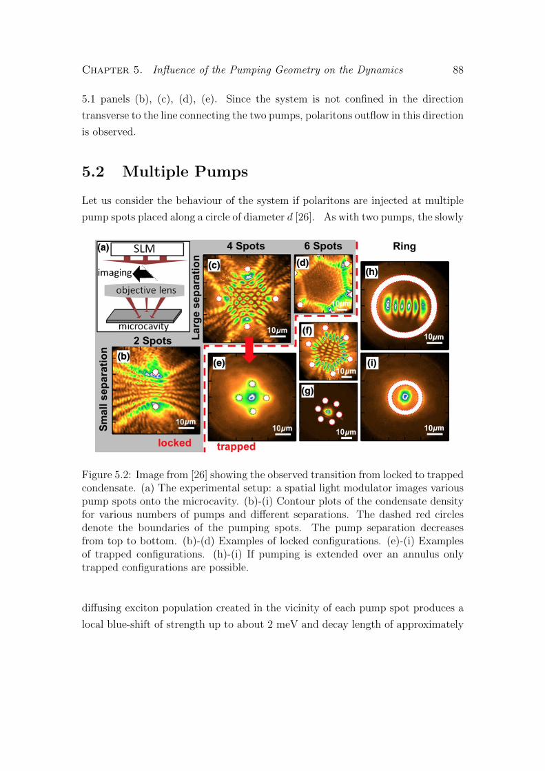
Chapter 5. Influence of the Pumping Geometry on the Dynamics 88
5.1 panels (b), (c), (d), (e). Since the system is not confined in the direction
transverse to the line connecting the two pumps, polaritons outflow in this direction
is observed.
5.2 Multiple Pumps
Let us consider the behaviour of the system if polaritons are injected at multiple
pump spots placed along a circle of diameter d [26]. As with two pumps, the slowly
Figure 5.2: Image from [26] showing the observed transition from locked to trappedcondensate. (a) The experimental setup: a spatial light modulator images variouspump spots onto the microcavity. (b)-(i) Contour plots of the condensate densityfor various numbers of pumps and different separations. The dashed red circlesdenote the boundaries of the pumping spots. The pump separation decreasesfrom top to bottom. (b)-(d) Examples of locked configurations. (e)-(i) Examplesof trapped configurations. (h)-(i) If pumping is extended over an annulus onlytrapped configurations are possible.
diffusing exciton population created in the vicinity of each pump spot produces a
local blue-shift of strength up to about 2 meV and decay length of approximately

Chapter 5. Influence of the Pumping Geometry on the Dynamics 89
Figure 5.3: Figure from [26] showing the dependence of the power threshold on thenumber and geometry of pump spots. The different regimes are denoted by theRoman numerals I (pumps effectively overlapping, no trap), II (trapped configura-tion) and III (locked configuration). (a) Dependence of the condensation thresholdon the number of pumps and their separation. (b) Phase diagram from the numer-ical simulations (dashed lines). Colours correspond to the threshold values in (a).(c) Data replotted as injected power per spot vs nearest distance between pumpspots. (d) Condensation threshold vs number of pump spots. The pump spots arearranged along a circle of diameter d “ 50 µm.

Chapter 5. Influence of the Pumping Geometry on the Dynamics 90
4 µm. The resulting potential can be modelled by a sum of Gaussians centred at
the pump positions,
V pxq “ V0
Nÿ
i“1
exp
ˆ
´|x´ xi|
2
2l2d
˙
, (5.12)
where N is the total number of pumps, xi is the position of the centre of the i-th
pump, V0 » 2 meV is the depth of the trap at the centre of the pump spot and
ld is the characteristic length over which excitons diffuse. Condensates forming
in correspondence of the different pump spots are accelerated by this potential,
interact and phase-lock, forming a single coherent condensate.
The behaviour of the system is highly sensitive to the number of pumps and
their distances. In fact, if d is less then some critical distance dc „ 30 µm, the con-
densate flips from a freely flowing but phase-locked regime to a spatially trapped
configuration, see figures 5.2 and 5.3. A higher pumping power facilitates the
transition and a larger number of pumps leads to a larger value of dc.
For d ą dc the condensate is in the locked regime (III). The system is not
trapped and polaritons outflow is observed. The cooperative behaviour of conden-
sates produced at different spots is evident from figure 5.3, panel (c), which shows
how the power per pump needed to reach the condensation threshold is, for N ą 2,
less than the single pump value of 11 mW, and from figure 5.3, panel (d), which
shows a sublinear increase with N of the total power need to obtain condensation.
For d ă dc the condensate undergoes a turbulent phase in which vortices are
continuously nucleated and destroyed. If d is further reduced, the system enters
a new stable configuration, the trapped regime (II). The condensate is now fully
confined and no polariton outflow is observed. This regime can be clearly observed
in figure 5.3, panel (a), as a pronounced drop in the threshold power. Within
the trapped regime, larger values of d generate a higher variety of 2D harmonic
oscillator states, see figure 5.2 panels (f), (h), while smaller values of d lead to a
Gaussian-shaped ground state, see figure 5.2 panels (e), (g).
Finally, for even smaller distances (d ă 12 µm), the potentials generated at
different pump spots overlap so much that the resulting potential has no central
minimum, but rather expels the condensate (regime III). The transition to this

Chapter 5. Influence of the Pumping Geometry on the Dynamics 91
different behaviour shows up as an increase in the threshold power in figure 5.3,
panel (a). As expected, in the limit d Ñ 0 the power threshold becomes equal to
that of a single pump.
Figure 5.4: Image from [26] showing the shape of the trap for (a) N “ 3, (b)N “ 4, (c) N “ 6. Panels (d) - (e) show a cross section of the potentials (a) -(c) along a line passing through the trap centre (blue dashed line) and throughtwo neighbouring pumps (red dashed line). Black arrows mark the effective trapdepth.
Two extreme cases show a different behaviour: for N “ 2 no fully trapped
state is possible, while if pumping is extended to an annulus only the trapped
configuration is admitted.
The observed behaviour can be partly understood by looking at the shape of
the trap as a function of d and N . For a fixed value of d, the trap is very shallow
if N is small, see figure 5.4, and polaritons can easily leak out from the gaps in
between pumps. This, as can be seen in figure 5.3, panel (c), leads to an increase in
the power per pump needed to obtain polariton condensation. As N is increased,
the gaps in the trap close, and the centre of the trap acquires a deep potential
minimum of circular shape which better supports the trapped configuration. If
N is kept fixed and d is decreased the trap becomes shallower. Eventually the

Chapter 5. Influence of the Pumping Geometry on the Dynamics 92
different pumps overlap so much that the trap disappears completely and what is
left is a single potential hill.
Figure 5.5: Figure from [26]. Comparison between experimental data (a)-(c) andresults of numerical simulations (d)-(f). The intermediate regime occurring inpassing from the locked to the trapped regime is characterised by a chaotic dy-namics with vortices continuously forming and annihilating. Experimental imagesare averaged over time and cannot show the dynamics of individual vortices. Tocompare with experiments, panel (e) shows dynamics averaged in time, while pan-els (d) and (f) show single snapshots of stationary configurations.
Quantum pressure plays a fundamental role in determining the transition from
locked to trapped configuration by preventing the condensate from accumulating
at the centre of the trap if d ą dc. Polariton outflows from different pumps create
standing waves whose wavelength ξ, which is inversely proportional to the veloc-
ity of the outflow, sets the length scale over which significant density fluctuations
occur. When pump spots are well separated the outflow velocity is large and ξ is
comparable with the healing length (2.39) of the system, which is approximately

Chapter 5. Influence of the Pumping Geometry on the Dynamics 93
1 µm. Quantum pressure is then important and, as revealed by numerical sim-
ulations, see figure 5.6 panels (c) and (d), generates a repulsive potential which
prevents the condensate from accumulating at the bottom of the trap. As pumps
get closer, the wavelength of density fluctuations becomes larger and quantum
pressure becomes negligible. At that point, the condensate accumulates in the
centre of the trap.
The experimental behaviour and the transition from locked to trapped regime
are well reproduced by numerical simulations of equation (2.32), see figure 5.5.
In the simulations, the potential caused by the repulsive interactions between
polaritons and reservoir excitons is modelled as Vextpxq “ V0 fpxq, with
fpxq “Nÿ
i“1
exp`
´wpx´ xiq2˘
, (5.13)
where w “ 0.03, matching the experimental diffusion length ld „ 4 µm. Polariton
gain, non-linear loss and relaxation are concentrated near the pumps and are best
fit by the choice of parameters
α “ fpxq, σ “ 0.3fpxq, η “ 0.1fpxq. (5.14)
The key role played by quantum pressure in the transition from locked to
trapped state can be clearly seen in figure 5.6: for d ą dc quantum pressure
generates a repulsive potential which prevents the condensate from reaching the
centre of the trap, see panel (c). As the distance between pumps is reduced the
quantum pressure contribution drops and the condensate density at the centre of
the trap increases, see panel (d).

Chapter 5. Influence of the Pumping Geometry on the Dynamics 94
Figure 5.6: Figure taken from [26]. Left: numerically obtained velocity profiles(grey scale and arrows) for the locked (a) and trapped (b) regimes. Red crossesdenote the pump positions ad white contours show the polariton density. Right:cross sections of (a) and (b) along the red dashed lines showing the pump-inducedpotential (V ), the quantum pressure (QP) and the condensate density (ρ). In (c)and (d) the blue dashed line marks the centre of the pump spot. Black arrowsshow the points at which the condensate density is highest.

Part II
Geometrical Models of Matter
95

Chapter 6
Background Material
Section 6.1 reviews some useful material on self-dual and Einstein manifolds. Sec-
tion 6.2 briefly introduces the geometrical models of matter framework [6]. Section
6.3, presents gravitational instantons, and in particular the ALF Ak´1 and ALF
Dk subclasses whose role as models for charged multi-particle systems is studied
in chapters 7 and 8. Other reference material has been put in appendix B.
6.1 Geometrical Preliminaries
In this section we briefly review the definitions of self-dual and Einstein manifolds
and some of their properties. A highly rigorous mathematical presentation can
be found in [12], while [66] is more in line with the notation and style used in
theoretical physics.
6.1.1 Self-duality
Let pM, gq be an oriented Riemannian manifold of dimension n. Denote by ΩppMq
the space of smooth differential p-forms on M . For α, β P ΩppMq denote by p, q
the product
pα, βq “ pβ, αq “1
p!αa1...apβ
a1...ap . (6.1)
The squared L2-norm ||α||2 of a p-form α is the positive definite quantity1
||α||2 “ pα, αq. (6.2)
The squared L2-norm of a vector-valued form is defined as the sum of the L2-norm
of its independent components. For example, the squared L2-norm ||R||2 of the
1We are assuming that M is a Riemannian manifold. For a Lorentzian manifold (6.2) is notpositive definite.
96

Chapter 6. Background Material 97
curvature 2-form R is given by
||R||2 “ÿ
aăb
||Rab||2“
ÿ
aăb
pRab,Rabq. (6.3)
The Hodge star operator ˚ : ΩppMq Ñ Ωn´ppMq, defined by2
α ^ ˚β “ pα, βq η, (6.4)
with η the canonical volume form of pM, gq, is an isomorphism between ΩppMq
and Ωn´ppMq. In components
p˚αqap`1...an “1
p!αa1...apηa1...apap`1...an . (6.5)
A form α is called self-dual (anti self-dual) if ˚α “ α (˚α “ ´α).
In four dimensions, ˚2|Ω2pMq “ Id. Therefore one has the decomposition
Ω2pMq “ Ω2`
pMq ‘ Ω2´pMq, (6.6)
where Ω2`pMq (Ω2´pMq) is the subspace of Ω2pMq consisting of self-dual (anti
self-dual) 2-forms. Note that reversing the orientation of M maps ˚ to p´1q ¨ ˚ and
therefore interchanges self-dual and anti self-dual forms.
Let M be a smooth manifold of dimension n. The tangent space E “ TpM at a
point p P M is a representation space for the structure group GLpEq „ GLpn,Rqof TM . The dual space E˚ is a representation space for the dual representation,
and the various tensor product spaces constructed out of E and E˚ are represen-
tation spaces for the appropriate tensor products of representations. If M has a
Riemannian structure it is possible to reduce the structure group from GLpn,Rqto Opnq. If M is also oriented, it is possible to further reduce it to SOpnq.
2Unfortunately different definitions of the Hodge star, differing by a sign, are used in theliterature.

Chapter 6. Background Material 98
The curvature 2-form R of a Riemannian oriented manifold M of dimension n,
R “ Rabeab eb “
1
2Rabcde
ab eb b ec ^ ed
“1
4Rabcde
a^ eb b ec ^ ed,
(6.7)
with Rabcd the components of the Riemann tensor, is at each point p P M an
element of S2pE ^ Eq, the vector space of p0, 4q tensors having the symmetries
Rabcd “ Rcdab, Rabcd “ ´Rbacd, Rabcd “ ´Rabdc. (6.8)
In addition, it satisfies the Bianchi identity
Rapbcdq “ 0, (6.9)
where parentheses denote symmetrisation with respect to the enclosed indices.
Denote by CE the subspace of S2pE^Eq which satisfies properties (6.8), (6.9).
For n ě 4, we have the following orthogonal decomposition of CE into Opnq-
irreducible modules [12],
R “ R
2npn´ 1qg ¯g `
1
n´ 2g ¯z `W , (6.10)
where W is the Weyl tensor, R is the scalar curvature, z is proportional to the
trace-free Ricci tensor and
ph ¯kqabcd “ hackbd ` kachbd ´ habkcd ´ kabhcd. (6.11)
In components,
Rabcd “R
npn´ 1qpgacgbd´gabgcdq`
`
gaczbd`zacgbd´gabzcd´zabgcd˘
`Wabcd, (6.12)
with Rab “ Rcacb the Ricci tensor, R “ Ra
a the scalar curvature and
zbd “1
n´ 2
ˆ
Rbd ´R
ngbd
˙
. (6.13)

Chapter 6. Background Material 99
The decomposition (6.10) is also SOpnq-irreducible if n ą 4. If n “ 4 it
is possible to further decompose the Weyl tensor into its self-dual and anti self-
dual parts W˘. A self-dual manifold (anti self-dual manifold)3 is an oriented
Riemannian 4-manifold with self-dual (anti self-dual) Weyl tensor, ˚Wab “ Wa
b
(˚Wab “ ´Wa
b). In components,
1
2Wa ef
b ηefcd “ ˘Wabcd. (6.14)
A conformally flat manifold, i.e. whose Weyl tensor vanishes, is obviously self-
dual. Another class of self-dual manifolds, which will be of interest for us later, are
hyperkahler 4-manifolds. A hyperkahler manifold is a complex manifold M which
admits covariantly constant complex structures I, J , K satisfying the quaternionic
relations I2 “ J2 “ K2 “ ´1, IJ “ ´JI “ K, JK “ ´KJ “ I,KI “ ´IK “ J
and such that the metric is Hermitian with respect to I, J , K.
6.1.2 Einstein Manifolds
An Einstein manifold is a Riemannian manifold pM, gq whose Ricci tensor Rab
satisfies
Rab “ k gab, (6.15)
with k P R a constant. Einstein manifolds are homogeneous at the curvature level
and can be viewed as the higher dimensional analogues of surfaces with constant
Gaussian curvature.
The scalar curvature R “ Raa of an Einstein manifold of dimension n is the
constant R “ k n. If k “ 0 then M is called Ricci-flat. 4-dimensional hyperkahler
manifolds are Ricci flat [12].
The following theorem, a proof of which can be found in [12], is used in the
classification of compact gravitational instantons discussed in section 6.3.
Let M be a compact self-dual Einstein manifold with scalar curvature R.
• If R ą 0, then M is isometric to S4 with the round metric or to CP 2 with
3In the mathematical literature, a manifold with self-dual Weyl tensor is also known as halfconformally flat. In the physical literature, the term self-dual manifold often refers to a manifoldhaving a self-dual Riemann tensor.

Chapter 6. Background Material 100
the Fubini-Study metric.
• If R “ 0, then M is either flat or its universal covering is a K3 surface with
the Calabi-Yau metric.

Chapter 6. Background Material 101
6.2 Geometric Models of Matter
The name of this section is taken from the 2012 paper [6] where the idea of mod-
elling particles with 4-dimensional manifolds has been first presented. This section
is not meant to be exhaustive, but only to summarise those ideas and notions that
will be referred to in the following chapters. Some discussion of the physical and
mathematical motivations for the model hypotheses is given in chapter 9.
According to [6], a particle is described by a 4-dimensional Riemannian oriented
manifold. The four dimensions are purely spatial. Time, and therefore dynamics,
still need to be included in the picture. The manifold is also assumed to be
complete, self-dual and Einstein.
If the particle is electrically charged, then its modelling manifold is non-compact
and describes not only the particle, but also the empty space in which the particle
resides. In order to recover the usual description of empty 3-space, flat R3, the
manifold is required to approach asymptotically a circle fibration over R3 (or its
quotient by some finite group).
If the particle is electrically neutral, the modelling manifold is instead supposed
to be compact. In order to describe how the particle sits in empty space it is
necessary to fix a preferred embedded 2-surface S where the 4-manifold intersects
physical 3-space. The surface S appears as the “boundary” of the particle for an
external observer.
Conserved quantum numbers of a particle are encoded in the topology of the
modelling manifold. In particular, if M models an electrically charged particle,
the self-intersection number of the base of its asymptotic fibration gives minus
the electric charge. It was initially proposed that the signature of M represents
the baryon number of the modelled particle, however, as remarked in [36], this
identification is not believed to hold anymore.
A manifold modelling an elementary particle is supposed to be rotationally
symmetric, therefore should has an SOp3q or SUp2q group of isometries. The
group action should preserve the extra structure: in the non-compact case it should
be asymptotically a bundle map covering the usual SOp3q action on R3, in the
compact case it should fix the preferred embedded 2-surface.
Concrete examples were made in [6] for a number of particles: the electron

Chapter 6. Background Material 102
is modelled by the Taub-NUT manifold [62], the proton by the Atiyah-Hitchin
manifold [5, 39], the neutron by CP 2 with the Fubini-Study metric.

Chapter 6. Background Material 103
6.3 Gravitational Instantons
A gravitational instanton is a 4-dimensional hyperkahler (therefore self-dual and
Ricci-flat) complete manifold. This definition is not universally agreed upon: some
authors insist that gravitational instantons are not compact. Some decay condition
is usually imposed on the curvature tensor of non-compact gravitational instantons,
typically that the L2-norm of the curvature 2-form is finite.
Gravitational instantons have been first considered by Hawking in an attempt
to construct a theory of quantum gravity analogous to Yang-Mills gauge theories
[46].4 In gauge theories self-dual solutions of the Yang-Mills equations, like BPST
instantons, are particularly important since they are absolute minima within their
topological type of the Yang-Mills action. The curvature 2-form of gravitational
instantons is self-dual5, therefore they also are absolute minima of the Yang-Mills
action. However, this fact is not as important as in Yang-Mills theories, where the
field equations are derived from the Yang-Mills functional, since the field equations
obeyed by the curvature 2-form of an Einstein manifold are not derived from the
Yang-Mills functional, but rather from the Euclidean Hilbert-Einstein action
ż
M
˚R, (6.16)
with R the scalar curvature of M .
Using the theorem reported in section 6.1.2, the classification of compact grav-
itational instantons is quickly obtained: the only compact hyperkahler manifolds
are, up to a finite covering, diffeomorphic to the flat torus or a K3 surface.
In the non-compact, topologically finite case, all known gravitational instantons
fall into four categories characterised by the asymptotic behaviour of the metric:
ALE, ALF, ALG and ALH. It is conjectured that all gravitational instantons fall
into one of these families [19].
4Note that the current definition of a gravitational instanton is slightly different from theoriginal one given by Hawking. As a consequence, manifolds like the Euclidean Schwarzschildsolution, which is not self-dual, are not considered gravitational instantons any more.
5As discussed in section 6.1.1, gravitational instantons are self-dual manifolds according tomathematicians’ use of the term: the Weyl tensor is self-dual. However, since they are alsoRicci-flat, the Riemann tensor reduces to the Weyl tensor.

Chapter 6. Background Material 104
In order to present the different families, we first need to give some details on
the topological and metric structure of gravitational instantons [33, 45]. Consider a
compact connected orientable 4-manifold M with connected boundary BM . Then
M “M z BM admits a decomposition M “ C Y N where C is a compact subset
of M and N is diffeomorphic to the open annulus BM ˆ p0,8q. Assume that BM
is the total space of a smooth fibration π : BM Ñ B with fibre F . Let x be a
boundary defining function, i.e. x “ 0, dx ‰ 0 on BM . Set r “ 1x and consider
the behaviour of the metric tensor g in a neighbourhood U of BM . The metric of
ALF gravitational instantons is of fibred boundary type, that is
g “ dr2` r2π˚h` k (6.17)
in U , with h a metric tensor on B and k a symmetric tensor on BM which restricts
to a metric tensor on each fibre F . In order for the curvature decay condition
to be satisfied, k must be a flat metric on F so that F is a connected compact
orientable flat manifold.
A simple example is given by the gravitational instanton A0 of the ALF family.
As discussed in section 6.3.1, ALF A0 has the topology of R4, which can be decom-
posed as R4 “ t0uY pS3 ˆ p0,8qq. The manifold S3 is the total space of the Hopf
fibration, discussed in 7.1.2, which has base S2 and fibre S1. Therefore, in the
notation used above, M is a 4-ball, BM “ S3, M “ R4, C “ t0u, N “ S3ˆp0,8q,
B “ S2, F “ S1.
The classification of non-compact gravitational instantons is based on the di-
mension of F :
• M is ALE (asymptotically locally Euclidean) if dimpF q “ 0.
• M is ALF (asymptotically locally flat) if dimpF q “ 1. Then F is diffeomor-
phic to S1.
• M is ALG (by induction) if dimpF q “ 2. Then F is diffeomorphic to the
2-torus.
• M is ALH (again by induction) if dimpF q “ 3. Then F is diffeomorphic to
one of the 6 flat orientable 3-manifolds.

Chapter 6. Background Material 105
A characterisation in terms of volume growth can also be given [20, 61]. The
volume growth of a geodesic ball of radius r is proportional to
• r4 for ALE manifolds,
• r3 for ALF manifolds,
• ra, 2 ď a ă 3 for ALG manifolds,
• ra, a ă 2 for ALH manifolds.
Only ALF gravitational instantons have the asymptotic properties required to
model a particle. We consider them in more detail in section 6.3.1.
In the following we will often make use of the Hausel-Hunsicker-Mazzeo com-
pactification XM of a gravitational instanton M which is obtained by collapsing
the fibres of M at infinity [45]. Equivalently, XM “M Y S where S is a 2-surface
diffeomorphic to the base of the asymptotic fibration of M . It is natural to think
of S as representing the spatial infinity of M .
In general XM is a stratified space, but if fibres are topologically 2-spheres, as
happens for ALF gravitational instantons, then XM is a manifold [45].
To continue with the example of ALF A0, which is homeomorphic to C2, in
agreement with the relation CP 2 “ C2YCP 1 we have XA0 “ CP 2, S “ CP 1 „ S2.
6.3.1 ALF Gravitational Instantons
All known ALF gravitational instantons fall into two infinite subfamilies, indexed
by a non-negative integer k: of type Ak and of type Dk. It is conjectured that
these two families exhaust the ALF class of gravitational instantons [19].
Topology
The Ak´1, k ě 1 and Dk, k ě 3, manifolds arise as the minimal resolution of
Kleinian singularities of cyclic and dihedral type, i.e. as a particular desingulari-
sation of the quotient of C2 by the action of a finite subgroup Γ of SU(2).
The finite subgroups of SUp2q are the cyclic group Zk of order k, the binary
dihedral group D˚k of order 4k, the binary tetrahedral group of order 24, the

Chapter 6. Background Material 106
binary octahedral group of order 48 and the binary icosahedral group of order
120. It is interesting to note that while there are ALE gravitational instantons
corresponding to all the possible finite subgroups of SUp2q [56], there are ALF
gravitational instantons corresponding only to the cyclic (type Ak´1) and binary
dihedral (type Dk) subgroups.
ALE and ALF gravitational instantons of the same class have the same topol-
ogy, but differ at the metric level. Topologically, they retract onto a configuration
of 2-spheres intersecting according to the Cartan matrix of the corresponding Lie
algebra. Outside a compact set containing these 2-spheres they are homeomorphic
to C2Γ where Γ “ Zk for Ak´1, k ě 1 and Γ “ D˚k´2 for Dk, k ě 3.6 This gives
large r hypersurfaces the structure of a circle bundle. The bundle structure will be
important for the calculation of the electric charge and will be examined in more
detail in chapter 7.
Small values of k need a separate description: A0, also known as the Taub-
NUT manifold, has the topology of C2; D0 retracts onto RP 2 and is not simply
connected; D1 retracts onto S2; D2 is the minimal resolution of singularities of
pR3 ˆ S1qZ2. Outside a compact set, the asymptotic topologies of D0 (D1) and
D4 (D3) are the same, but the orientation is opposite [13].
Topological Invariants
Let us compute the Euler number χ and the signature τ of ALF gravitational
instantons. A definition of these quantities is given in appendix B.1.
The Euler number χpMq of a manifold M can be calculated as the alternating
sum of the Betti numbers bipMq “ dim pH ipMkqq of M . The de Rham cohomology
groups of an ALF gravitational instanton are
HppMkq “
$
’
’
’
&
’
’
’
%
R if p “ 0,
Rk if p “ 2,
0 otherwise,
(6.18)
6Not that D˚1 „ Z4. However the Z4-actions on the A3 and D3 manifolds are different.

Chapter 6. Background Material 107
where Mk is either Ak, k ě 0, or Dk, k ě 1. Hence
χpMkq “
4ÿ
i“1
bipMkq “ k ` 1. (6.19)
We can double check the value of χpAkq using the generalised Gauss-Bonnet
theorem (B.3). Since the integral of the curvature form over Ak, calculated in
appendix B.4, isż
Ak
||R||2 η “ 8π2pk ` 1q , (6.20)
and there are no boundary contributions, we verify that χpAkq “ k ` 1. It is
interesting to note that, since χpDkq “ χpAkq, the integral of ||R||2 η over Dk is
also given by 8π2pk ` 1q.
The signature τpMq of a manifold is
τpMq “ dim`
H2`pMq
˘
´ dim`
H2´pMq
˘
, (6.21)
where H2`pMq (H2´pMq) is the subspace of H2pMq consisting of self-dual (anti
self-dual) forms, see appendix B.1 for more details. The sign of τpMq depends on
the orientation chosen on M . Our choices of orientation for Ak and Dk are given
in (6.47) and (6.48).
Signature can be also calculated as the integral of a polynomial in the curvature
2-form. For a manifold M with self-dual curvature 2-form, Hirzebruch’s signature
theorem (B.10) gives
τpMq “1
12π2
ż
M
||R||2 η ` b. d., (6.22)
where b. d. stands for the contribution from the boundary at infinity. For both
Ak and Dk gravitational instantons the boundary contribution is pk ´ 2q3, see
(B.14), therefore
τpMkq “ pk ´ 2q3` 2pk ` 1q3 “ k, (6.23)
where Mk is either Ak or Dk.
As noted in [36], according to the original proposal [6] τpMq gives the baryon
number of the particle modelled by M . For both Ak and Dk, τ “ k. The fact

Chapter 6. Background Material 108
that, for k ą 0, the signature of Ak does not agree with the baryon number of a
system of k ` 1 electrons suggested dropping the identification of signature with
baryon number.
Hausel-Hunsicker-Mazzeo Compactification
The topology of the Hausel-Hunsicker-Mazzeo compactification of ALF Ak´1 grav-
itational instantons has been calculated in [33]. The result is given by the following
theorem.
Let pM, gq be an ALF gravitational instanton such that one of its Kahler forms
ω “ dβ is exact and its Hausel-Hunsicker-Mazzeo compactification XM is simply
connected. Take on XM the orientation induced by any of the complex struc-
tures on pM, gq. Let k “ dim pL2H2pMqq, where L2H2pMq is the space of square-
integrable harmonic 2-forms on M , then there is a homeomorphism of oriented
topological manifolds
XM „
#
S4 if k “ 0,
#k CP2 otherwise,(6.24)
where #k CP2 is the connected sum of k complex projective planes taken with the
orientation opposite to the one induced by the standard complex structure. The
case XM “ S4 is realised by the flat space R3 ˆ S1 while the compactification of
Ak´1 is #k CP2 [33].
The compactification of the Atiyah-Hitchin manifold, and therefore of D1,
which differs from the Atiyah-Hitchin manifold only at the metric level, is CP 2,
the compactification being achieved by gluing an RP 2 at infinity [6]. The compact-
ification of Dk is likely to be the connected sum of k complex projective planes,
but this has not been proved yet.
The Gibbons-Hawking Ansatz
Coming to the metric structure of ALF gravitational instantons, both the exact
Ak´1 and the asymptotic Dk metrics can be expressed in the form known as the

Chapter 6. Background Material 109
Gibbons-Hawking ansatz [37],
ds2“ V pdr2
` r2dΩ2q ` V ´1
pdψ ` αq2 , (6.25)
where dΩ2 “ dθ2 ` sin2 θ dφ2, r P r0,8q, θ P r0, πs, φ P r0, 2πq are spherical
coordinates and ψ is an angle whose range depends on the precise form of V . Note
that the metric dr2 ` r2dΩ2 is the flat metric on R3. The 1-form α is locally such
that dα “ ˚3dV , with ˚3 the Hodge dual with respect to this flat metric. More
explicitly
BxV “ Byαz ´ Bzαy,
ByV “ Bzαx ´ Bxαz,
BzV “ Bxαy ´ Byαx.
(6.26)
It follows that V is a harmonic function.
The Gibbons-Hawking ansatz gives a self-dual metric. This is a consequence
of the following result. Let pM, gq be a Riemannian manifold, teiu an orthonormal
frame, teiu the orthonormal coframe and define the self-dual 2-forms
β1“ e4
^ e1´ e2
^ e3, β2“ e1
^ e3´ e2
^ e4, β3“ e4
^ e3´ e1
^ e2. (6.27)
If dβi “ 0 for i “ 1, 2, 3, then (M , g), with
g “ e1b e1
` e2b e2
` e3b e3
` e4b e4, (6.28)
is a hyperkahler manifold, hence self-dual with respect to the orientation opposite
to the one induced by the complex structure [32]. Note that the 2-forms tβiu form
a basis for the space of self-dual 2-forms.
An orthonormal basis of the cotangent space with respect to the metric (6.25)
is given by
e1“?V dx, e2
“?V dy, e3
“?V dz, e4
“1?Vpdψ ` αq . (6.29)

Chapter 6. Background Material 110
Since, for example,
dβ1“ dα ^ dx´ dV ^ dy ^ dz “
´
pByαz ´ Bzαyq ´ BxV¯
dy ^ dz ^ dx
“
´
pdα ´ ˚3dV qyz dy ^ dz¯
^ dx “ 0,(6.30)
it follows that the closure condition for the 2-forms βi is equivalent to the relation
dα “ ˚3dV. (6.31)
p2p1
p3
p
p1 p2
p3
1Ak
1Ak
R3 1Ak
Figure 6.1: The structure of an Ak ALF gravitational instanton illustrated fork “ 3. The manifold Ak can be viewed as the union of a circle bundle over R3ztpiuand k ` 1 points tpiu. The inverse image by πAk of several subsets of R3 is shownin the figure in cyan colour. The inverse image of the NUTs p1, p2, p3 is a singlepoint, while the inverse image of an ordinary point p is a circle. The inverse imageof a line connecting two NUTs, the dashed line between p1 and p2 in the figure,is a cylinder with the circles at both ends collapsed to a point, topologically a2-sphere.

Chapter 6. Background Material 111
Ak´1 metric
The metric of the Ak´1 family, whose members are also known as multi Taub-NUT
gravitational instantons [37], is
ds2“ V
`
dr2` r2dΩ2
˘
` V ´1pdψ ` αq2 (6.32)
with
V “ 1`kÿ
i“1
µ
||p´ pi||, (6.33)
where µ ą 0 is a constant. The point p has spherical coordinates pr, θ, φq and tpiu
are the positions of k distinct points in R3, the NUTs. If px, y, zq are the Cartesian
coordinates of the point p and pxi, yi, ziq are the Cartesian coordinates of pi, then
||p´ pi|| “a
px´ xiq2 ` py ´ yiq2 ` pz ´ ziq2.
In order for (6.32) to be free from conical singularities, ψ needs to have the
range ψ P r0, 4πµq. In fact the metric near a NUT is approximately that of single
Taub-NUT,
ds2„
´
1`µ
r
¯
`
dr2` r2dΩ2
˘
`
´
1`µ
r
¯´1
pdψ ` µ cos θ dφq2 , (6.34)
with r the distance from the NUT. Substituting r “ ρ2p4µq one obtains
ds2„ dρ2
`ρ2
4
`
dΩ2` pdpψµq ` cos θ dφq2
˘
, (6.35)
which, provided that ψµ P r0, 4πq, is the flat metric on R4 expressed in terms of
the radial variable r and the Euler angles ψµ, θ, φ on SUp2q.
Geometrically a NUT is a fixed point of the action of the Killing vector BBψ
on the manifold [38]. Excluding the NUTs Ak is a circle bundle over R3, with a
projection πAk mapping each circle to its base-point in R3. We can extend πAk to
a map, which we will denote by the same symbol, defined on the whole of Ak by
letting it act trivially on the NUTs. A schematic picture of Ak and of the action
of πk is given in fig. 6.1.
Note that an ALF Ak gravitational instanton has k ` 1 NUTs. Since it is
notationally more convenient to deal with k NUTs we frequently work with Ak´1

Chapter 6. Background Material 112
instead of Ak.
The metric of the Dk family is, with the exception of D0 and D1, known only
implicitly [21]; the D2 metric is presented as an approximation to the K3 metric in
[47]. However, for large r the following asymptotic approximation is known [18]:
ds2“ V
`
dr2` r2dΩ2
˘
` V ´1pdψ ` αq2 , (6.36)
with
V “ 1´2µ
||p||`
kÿ
i“1
µ
2
ˆ
1
||p´ pi||`
1
||p` pi||
˙
. (6.37)
In (6.37) t˘piu are 2k distinct points in R3, dα “ ˚3dV , θ P r0, πs, φ P r0, 2πq,
ψ P r0, 2πµq, and there is the additional Z2 identification
pθ, φ, ψq „ pπ ´ θ, φ` π,´ψq. (6.38)
Note that (6.37) is given by the superposition of a NUT of negative weight located
at the origin and 2k NUTs at t˘piu, and is symmetric under inversion in the origin.
Close to each NUT pi the metric (6.36) is well approximated by the A0 metric.
For r Ñ 8 the positions of the NUTs become irrelevant and the metric has
the leading asymptotic form (6.36) with V given by
V “ 1`pk ´ 2qµ
r, (6.39)
where r “ ||p||.
If all the NUTs are very distant from the origin then (6.37), at large distances
from both the origin and the NUTs, i.e. for 0 ! r ! ||pi||, reduces to
V „ 1´2µ
r(6.40)
The metric (6.36) with V given (6.40) is the asymptotic form of the D0 metric.
Therefore, if all the NUTs are far from the origin, Dk resembles a central D0
surrounded by 2k A0-like NUTs.
From the moduli space description of Dk [22, 23] follows that it is possible to
set pk “ 0 without making the manifold singular or altering its topology. Doing

Chapter 6. Background Material 113
so, equation (6.37) becomes
V “ 1´µ
||p||`
k´1ÿ
i“1
µ
2
ˆ
1
||p´ pi||`
1
||p` pi||
˙
. (6.41)
If the other 2pk ´ 1q NUTs are far from the origin, then (6.41), at large distances
from both the origin and the NUTs, i.e. for 0 ! r ! ||pi||, i ‰ k, reduces to
V „ 1´µ
r. (6.42)
The metric (6.36) with V given by equation (6.42) is the asymptotic form of
the Atiyah-Hitchin metric, the maximally symmetric member of the D1 family.7
Therefore, if a pair of NUTs sits at the origin and all the other are far from it, Dk
resembles a central Atiyah-Hitchin manifold surrounded by 2pk´1q A0-like NUTs.
The parameter µ has the physical dimensions of a length and is related to the
length of the circles in the asymptotic fibration which is 4π µ for Ak´1 and 2π µ
for Dk. It is natural to choose the value of µ so that the asymptotic length of the
circles is 2π, that is
µ “
$
&
%
12
for Ak´1,
1 for Dk.(6.43)
We anticipate here that with the choice (6.43) of µ asymptotically
pdψ ` αqAk´1“ ωk, (6.44)
pdψ ` αqDk “ ω2pk´2q, (6.45)
see equations (7.48), (7.55). In (6.44) pdψ ` αqAk´1is the 1-form comparing in
the Ak´1 metric (6.32); in (6.45) pdψ ` αqDk is the (different) 1-form comparing
in the asymptotic Dk metric (6.36). In both cases ωl is given by the 1-form (7.41)
discussed in chapter 7.
7The D1 family, whose asymptotic metric is parametrised by p1, has been studied by Dancer[27]. Members of the D1 family generally have only a Up1q group of isometries. The Atiyah-Hitchin manifold is obtained for p1 “ 0 and has instead an SOp3q group of isometries.

Chapter 6. Background Material 114
Orientation
A Kahler 4-manifold with Kahler form β has a canonical orientation, β^β, induced
by its complex structure. A hyperkahler manifold has three Kahler forms β1, β2,
β3, but they all induce the same orientation. For Ak, these forms are given by
(6.27), and the induced orientation is, in (r, ψ, θ, φ) coordinates,
β1^ β1
“ β2^ β2
“ β3^ β3
“ 2V r3 sin2 θ dr ^ dθ ^ dφ^ dψ. (6.46)
We want to take the orientation opposite to the one induced by the complex
structure. For Ak it is
orAk “ dψ ^ dr ^ dθ ^ dφ. (6.47)
For Dk it is
orDk “ dr ^ dψ ^ dθ ^ dφ. (6.48)

Chapter 7
Asymptotic Topology and Charge
According to [6], there are two different definitions of the electric charge of a
particle modelled by a non-compact manifold M . The first one is minus the self-
intersection number of the surface representing infinity in the Hausel-Hunsicker-
Mazzeo compactification XM of M . More precisely, if S is the base of the asymp-
totic fibration, and therefore XMzS “ M , then charge is given by minus the self-
intersection number of S in XM . The second definition is minus the first Chern
number of the asymptotic circle fibration of M .
The two definitions are equivalent provided that the asymptotic fibration is
oriented, i.e. provided that the structure group is Up1q „ SOp2q. This is the
case for the Ak´1 family. However, if the asymptotic fibration is not oriented, as
happens for the Dk family, then it is not possible to define its first Chern number
C1. However, it is possible to construct a double cover Dk of Dk which has an
oriented asymptotic fibration. Charge can be then computed as minus one half of
the first Chern number of the double cover asymptotic fibration.
While the charge definition in terms of the self-intersection number is more
satisfactory as it applies to both families without the need of any additional con-
struction, the definition in terms of C1 is closer to physics as it can be viewed as a
generalisation of Gauss’ flux theorem. For this reason, I have chosen to compute
the electric charge of Ak´1 and Dk by calculating the first Chern number of the
relevant fibration, as I originally did in [36].
Section 7.1 contains a detailed explanation of the charge definition in terms
of C1. Section 7.2 illustrates the charge computation for Ak´1 and Dk. The
equivalence between the two charge definitions in the case of Ak´1 gravitational
instantons is discussed in appendix B.2. Some background material on principal
bundles and characteristic classes has been summarised in appendix B.3.
115

Chapter 7. Asymptotic Topology and Charge 116
7.1 Definition
7.1.1 Motivation
The dynamical Maxwell equations for an electric field E, in 3-dimensional vector
notation, are
∇ ¨ E “ 4πρe. (7.1)
The electric charge Qe contained in a volume V is then
Qe “
ż
V
ρe dV “1
4π
ż
V
∇ ¨ E dV “1
4π
ż
BV
E ¨ dσ, (7.2)
where dV and dσ are the natural volume elements of V and BV , the latter taken
with the orientation induced by the external unit vector perpendicular to BV .
If the volume V is the whole of R3, we can consider its “boundary” to be the
2-sphere at infinity S28 “ limRÑ8 S
2R. Therefore electric charge can be calculated
by integrating the flux of E at infinity,
Qe “1
4π
ż
S28
E ¨ dσ. (7.3)
Since in [6] the roles of electric and magnetic fields are reversed, electric charge
is given by the appropriate generalisation of a relation similar to (7.3) but involving
the magnetic field B. Let us then consider the behaviour of a particle having non-
zero magnetic charge. The magnetic field generated by a point particle of magnetic
strength g is
B “g
r3r. (7.4)
Because of the radial direction of B in (7.4) and the r´2 dependence of its modulus,
one can apply Gauss theorem and relate the magnetic charge contained in a volume
V with the flux of B obtaining an expression exactly analogous to (7.3).
However, a fundamental property of electric charge is its quantisation. We will
derive below the Dirac quantisation condition which states that, for a monopole
of strength g and an electrically charged particle of charge q, in units such that
the charge of the proton is one, the condition 2 qg P Z must hold. Therefore, if q
is integer, 2g, rather than g, is also an integer. For this reason, it is preferable to
Chapter 7. Asymptotic Topology and Charge 117
define the magnetic charge of a monopole of strength g to be 2g, and the analogous
of (7.3) reads
Qm “1
2π
ż
S28
B ¨ dσ. (7.5)
For future use, we would like to rewrite (7.5) in a more geometrical form. In
order to do this, it is convenient to make use of the exterior calculus formalism.
Let B “ B5 be the 1-form associated to the magnetic field B via the canonical iso-
morphism induced by the flat metric gp3q on R3, F “ ˚3B be the 2-form1 obtained
applying the Hodge operator induced by gp3q on B. If Ba are the components of
B with respect to a coordinate basis tBBxau, then
B “ Bbgp3qab dxa, F “
1
2
b
detpgp3qqBc εcab dxa ^ dxb, (7.6)
where εabc is the Levi-Civita symbol in three dimensions.
For the magnetic field of a point particle (7.4), using spherical coordinates
r, θ, φ, we have
B “g
r2dr, F “ g sin θ dθ ^ dφ, (7.7)
therefore (7.5) can be rewritten simply as
Qm “1
2π
ż
S28
F. (7.8)
The 2-form F is closed, i.e. dF “ 0, but not exact2, i.e. it cannot be written
as the exterior derivative of a globally defined 1-form. In fact, suppose there were
a globally defined 1-form A such that F “ dA. Then, using Stokes’ theorem, we
would have
2π Qm “ limRÑ8
ż
S2R
dA “ limRÑ8
ż
BS2R
A “ 0, (7.9)
in contradiction with the fact that the particle has magnetic charge 2g as one
readily obtains by directly calculating the integral (7.8).
1The 2-form F is the usual electromagnetic field-strength 2-form of a stationary magneticfield in a frame where the electric field vanishes.
2Indeed F is 4πg times the canonical volume form of S2, which is homotopically equivalentto R3zt0u, therefore it is a non-trivial element of H2
`
R3zt0u˘
.

Chapter 7. Asymptotic Topology and Charge 118
However, it is possible to locally express F as the exterior derivative of a 1-
form. Since F does not depend on the radial variable r, it is convenient to work
on S2, and introduce the two gauge potentials
AN
AS
+
“ ´g pcos θ ¯ 1q dφ, (7.10)
with AN singular for θ “ π, AS singular for θ “ 0. The exterior derivative of both
AN and AS is F .
If we work with the local potentials AN and AS, Stokes’ theorem applied to
(7.8) yields the right result. Write SN for the upper hemisphere of S28 and SS for
the lower hemisphere, so that SN Y SS “ S28, SN X SS “ S1. Note that both SN
and SS have S1 as their boundary, but with opposite orientations. Then
Qm “1
2π
ż
S28
F “1
2π
ż
SN
dAN `1
2π
ż
SS
dAS
“1
2π
ż
BSN
AN `1
2π
ż
BSS
AS “1
2π
ż
S1
pAN ´ ASq
“1
2π
ż
S1
2g dφ “ 2g.
(7.11)
We can now derive Dirac’s quantisation condition. Consider the wave func-
tions ψN and ψS, defined on SN and SS, of a particle with electric charge e. Since
AN “ AS ` 2g dφ, the wave functions ψN and ψS are related by the gauge trans-
formation ψN “ ψS expp2i eg φq. In order for ψN to be single-valued, working in
units such that e “ 1, we must have 2g “ l P Z.
The adequate generalisation of (7.8) to the more complicated topologies of ALF
gravitational instantons is given by minus the first Chern number of the asymptotic
fibration of these manifolds, to be discussed in the next section.
7.1.2 Formalisation
Some background material on connection on principal bundles has been discussed
in appendix B.3, for more details see [64], [65] or [66].
Manifolds modelling charged particles have asymptotic hypersurfaces with the

Chapter 7. Asymptotic Topology and Charge 119
topology of a circle bundle P over a boundaryless 2-surface S. Provided that the
structure group of P is Up1q, the appropriate generalisation of (7.8) is ´C1pP q,
where C1pP q, the first Chern number of P , is given by3
C1pP q “ ´1
2π
ż
S
F. (7.12)
In (7.12) F is the field strength associated to any connection on P .
According to [6], in the geometric models of matter framework the roles of
electric and magnetic fields are reversed, so it is the electric charge Q to be given
by ´C1pP q.
Let us see how the formalism works in the case of the Hopf bundle PH , a Up1q-
bundle over S2 with total space S3. We will see in the next section that the Hopf
bundle models the asymptotic structure of A0, the manifold describing an electron.
Consider S3 as a submanifold of C2, S3 “ tpz1, z2q P C2 | |z1|2 ` |z2|2 “ 1u. The
Hopf projection π : S3 Ă C2 Ñ S2 is the restriction to S3 of the surjective map4
pz1, z2q ÞÑ
`
2Re`
z1z2˘
, 2Im`
z1z2˘
, |z1|2´ |z2
|2˘
. (7.13)
Points with the same ratio z1z2 are mapped to the same point of S2. This gives
S3 the structure of a Up1q-bundle over S2 with projection π and right action
σ : S3 ˆ Up1q Ñ S3 given by complex number multiplication:
σ`
pz1, z2q, exppiwq
˘
“ pz1 exppiwq, z2 exppiwqq. (7.14)
In order to calculate C1pPHq using (7.12) we need to define a connection ω
on PH . As discussed in appendix B.3, for each u P PH the tangent space VuPH
3The definition (7.12) of the first Chern number is only valid for principal bundles with anAbelian structure group. For such bundles the field strength F is a globally defined 2-form onS. The general case is discussed in appendix B.3.
4We recall that the Hopf projection π can be expressed in terms of the stereographic projectionfrom the north pole φN : S2 Ă R3 Ñ R2 as πpz1, z2q “ φ´1
N pz1z2q, with
φN px1, x2, x3q “
ˆ
x1
1´ x3,
x2
1´ x3
˙
, φ´1N pzq “
ˆ
2z
1` |z|2,|z|2 ´ 1
|z|2 ` 1
˙
P S2 Ă Cˆ R „ R3.
Chapter 7. Asymptotic Topology and Charge 120
to the fibre over u, known as the vertical space at u, can be defined without any
additional structure. However there is no canonical way of choosing a complement
HuPH of VuPH in TuPH . A connection on PH is equivalent to a smooth choice
of such a complement for all u P PH . The vector space HuPH is known as the
horizontal space at u.
Since different connections give the same first Chern number, we are free to
make a simple choice for ω. The embedding of S3 in C2 „ R4 given by the inclusion
suggests a natural choice for HuPH : the real orthogonal complement of VuPH in
TuPH with respect to the Euclidean metric on R4. Let u “ pu1, u2q P S3. The
vertical space at u is
VuPH “ tpu1, u2
qi w |u1, u2P C, w P up1q „ Ru. (7.15)
If a, b P C, their real inner product is given by Re pa bq. Therefore a P TuPH is
in the real orthogonal complement of VuPH provided that Re`
i uw a˘
“ 0 for all
w P R, i.e. if and only if Impu1a1 ` u2a2q “ 0. Therefore the horizontal space at u
is
HuPH “ Ker`
Impz1dz1` z2dz2
q˘ˇ
ˇ
u. (7.16)
The connection ω equivalent to the choice (7.16) of horizontal subspaces of
TuPH has, for each u P PH , HuPH as its kernel. It is therefore given by
ω “ r Im`
z1dz1` z2dz2
˘
, (7.17)
where r, a priori a real function of z1, z2, still needs to be determined.
In order to fix r, let us check the two properties which must be satisfied by
a connection form. As discussed in appendix B.3, the connection form ω on a
principal bundle P with structure group G and right action σ needs to satisfy
equations (B.33), (B.34) which for convenience we rewrite here5:
σ˚gω “ adg´1 ˝ ω, (7.18)
ωpw#q “ w, (7.19)
5Since the Lie algebra of Up1q is simply R, in passing from (B.34) to (7.19) we have switchedto a lowercase notation for its elements (W Ñ w).
Chapter 7. Asymptotic Topology and Charge 121
where g P G, w P g, w# is the fundamental vector field associated to w, σ˚gω
denotes the pullback of ω by σg “ σp¨, gq and adg denotes conjugation by g.
In our case P “ PH , G “ Up1q and σ is given by (7.14). Since Up1q is Abelian,
(7.18) reduces to the condition σ˚gω “ ω which is satisfied provided that r is
invariant under the Up1q-action, i.e. such that rpz1 exppiwq, z2 exppiwqq “ rpz1, z2q.
Equation (7.19) requires ω to act as the identity on the fundamental vector
field generated by an element w of g and therefore fixes the normalisation of ω.
Let t ÞÑ exppiwtq, with w P up1q „ R, be a curve on Up1q. The value of w# at u is
w#puq “
d
dt
ˇ
ˇ
ˇ
ˇ
t“0
σ`
u, exppiwtq˘
“d
dt
ˇ
ˇ
ˇ
ˇ
t“0
pu1, u2qeitw “ i pu1, u2
qw, (7.20)
where u “ pu1, u2q P S3, therefore
ωupw#puqq “ r Im
´
`
z1dz1` z2dz2
˘
ˇ
ˇ
ˇ
u
`
ipu1, u2qw
˘
¯
“ rRe`
u1u1w ` u2u2w˘
“ r`
|u1|2` |u2
|2˘
w “ r w.(7.21)
It follows r “ 1.
The connection on PH that we have found is therefore the 1-form
ω “ Im`
z1dz1` z2dz2
˘
, (7.22)
We now want to rewrite ω in a form which makes clear its relation with
the gauge potentials AN and AS given in (7.10). Introduce local coordinates
ψ P r0, 2πq, θ P r0, πs, φ P r0, 2πq on π´1 pS2ztpN , pSuq, where pS “ p0, 0,´1q

Chapter 7. Asymptotic Topology and Charge 122
is the south pole of S2 and pN “ p0, 0, 1q the north pole, via6
z1“ cos
ˆ
θ
2
˙
exp
ˆ
i
ˆ
ψ `φ
2
˙˙
,
z2“ sin
ˆ
θ
2
˙
exp
ˆ
i
ˆ
ψ ´φ
2
˙˙
.
(7.23)
In these coordinates the Hopf map is
pψ, θ, φq ÞÑ psin θ cosφ, sin θ sinφ, cos θq, (7.24)
and ω is given by
ω “ dψ `1
2cos θ dφ on π´1
`
S2ztpN , pSu
˘
. (7.25)
Expression (7.25) is not defined for θ “ 0, π. In order to get a globally defined
expression for ω we need to use two different coordinate patches, UN “ S2ztpSu,
US “ S2ztpNu. Defining the angles
ψN “ ψ `φ
2P r0, 2πq, ψS “ ψ ´
φ
2P r0, 2πq, (7.26)
we have
ω “
$
&
%
dψN `12pcos θ ´ 1qdφ on π´1 pUNq,
dψS `12pcos θ ` 1qdφ on π´1 pUSq.
(7.27)
Pulling back ω to UN , US via appropriately chosen cross-sections of PH we can
recover the gauge potentials (7.10).
The standard local trivialisations ΨN,S : π´1pUN,Sq Ñ UN,S ˆ S1 of the Hopf
6Usually the parametrisation (7.23) of S3 in terms of Euler angles is given by
z1 “ cos
ˆ
θ
2
˙
exp
ˆ
i
2
´
ψ ` φ¯
˙
,
z2 “ sin
ˆ
θ
2
˙
exp
ˆ
i
2
´
ψ ´ φ¯
˙
.
with ψ P r0, 4πq. Since it is convenient for us to fix the length of the asymptotic fibres of Ak´1
and Dk to be 2π, we prefer to work with an angle ψ in the range r0, 2πq.

Chapter 7. Asymptotic Topology and Charge 123
bundle are
ΨNppz1, z2
qq “ pπppz1, z2qq, ψNppz
1, z2qqq “
ˆ
πppz1, z2qq,
z1
|z1|
˙
,
ΨSppz1, z2
qq “ pπppz1, z2qq, ψSppz
1, z2qqq “
ˆ
πppz1, z2qq,
z2
|z2|
˙
,
(7.28)
with inverses
Ψ´1N
`
rz1, z2s, g
˘
“`
z1, z2˘ |z1|
z1g “
ˆ
|z1|, z2 |z
1|
z1
˙
g,
Ψ´1S
`
rz1, z2s, g
˘
“`
z1, z2˘ |z2|
z2g “
ˆ
z1 |z2|
z2, |z2
|
˙
g,
(7.29)
where rz1, z2s denotes a point in CP 1 „ S2 and g P S1.
The associated local cross-sections, see appendix B.3, sN,S : UN,S Ñ π´1 pUN,Sq
are
sNprz1, z2
sq “ Ψ´1N prz
1, z2s, 1q “
ˆ
|z1|, z2 |z
1|
z1
˙
,
sSprz1, z2
sq “ Ψ´1S prz
1, z2s, 1q “
ˆ
z1 |z2|
z2, |z2
|
˙
.
(7.30)
In terms of the angular coordinates (θ, φ)
sNpθ, φq “
ˆ
cos
ˆ
θ
2
˙
, sin
ˆ
θ
2
˙
e´iφ˙
,
sSpθ, φq “
ˆ
cos
ˆ
θ
2
˙
eiφ, sin
ˆ
θ
2
˙˙
.
(7.31)
Pulling back ω via sN,S one gets the local gauge potentials
pA1qN “ s˚Nω
pA1qS “ s˚Sω
+
“1
2pcos θ ¯ 1q dφ. (7.32)
with pA1qN singular for θ “ π, pA1qS singular for θ “ 0. Comparing (7.32) with
(7.10) we see that the gauge potentials (7.32) are equal to those of a magnetic
monopole of charge one (g “ 12).

Chapter 7. Asymptotic Topology and Charge 124
The curvature form Ω associated to the connection form ω is the 2-form
Ω “ dω “ ´1
2sin θ dθ ^ dφ.7 (7.33)
Pulling back F via sN,S one obtains the field strengths FS “ s˚S Ω, FN “ s˚N Ω.
Since FN “ FS on US X UN , we can define a 2-form F , globally defined on S2, as
F “
$
&
%
s˚S Ω on US
s˚N Ω on UN“ ´
1
2sin θ dθ ^ dφ. (7.34)
Let us finally compute the first Chern number of the Hopf bundle:
C1pPHq “ ´1
2π
ż
S2
F “1
4π
ż
S2
sin θ dθ dφ “ 1. (7.35)
7Note that Ω, a priori a 2-form on S3, is actually a 2-form globally defined on S2. Moreformally we should say that Ω “ π˚F , where F is a 2-form on S2 and π is the Hopf bundleprojection. This is not a coincidence: as discussed in appendix B.3, the curvature form of aprincipal G-bundle P over B can be identified with an (adP )-valued 2-form FΩ globally definedon B. If G is Abelian, then FΩ univocally determines a g-valued 2-form F globally defined onB.

Chapter 7. Asymptotic Topology and Charge 125
7.2 Ak´1 and Dk Charge and Particle Interpre-
tation
Let us start computing the electric charge of Ak´1. We first need to understand
the topology of large r hypersurfaces. If k “ 1, the topology is that of C2. A large
r hypersurface has the topology of S3 “ tpz1, z2q P C2| |z1|2 ` |z2|2 “ 1u which
is a circle bundle over S2, the Hopf bundle PH described in section 7.1.2. As we
calculated in (7.35), C1pPHq “ 1, therefore QA0 “ ´1.
If k ą 1, outside a compact set the topology is that of C2Zk, where the action
of Zk is generated by
pz1, z2q ÞÑ exp
ˆ
i2π
k
˙
pz1, z2q. (7.36)
Extend the coordinates (7.23) ψ P r0, 2πq, θ P r0, πs, φ P r0, 2πq to the whole of C2
introducing an additional radial variable r P r0,8q,
z1“ r cos
ˆ
θ
2
˙
exp
ˆ
i
ˆ
ψ `φ
2
˙˙
,
z2“ r sin
ˆ
θ
2
˙
exp
ˆ
i
ˆ
ψ ´φ
2
˙˙
.
(7.37)
Since the Zk-action generated by (7.36) leaves r invariant, we can focus on what
happens to a fixed, large r hypersurface. The ratio z1z2 is also left invariant by
the Zk-action, hence the Hopf fibration π descends to a map, which we will still
denote with π : S3Zk Ñ S2, and the base of the asymptotic fibration is still S2.
Because of the identification (7.36), ψ „ ψ`2πk, hence ψ is periodic with period
2πk. Therefore, the fibre is again a circle, but with length 2πk. In conclusion, for
all k ě 1, the topology of a large r hypersurface in Ak´1 is that of a Up1q-bundle
over S2.
In order to calculate C1, it is convenient to consider the following 1-form, which
appears in the asymptotic metrics of both Ak´1 and Dk and generalises (7.22),
ωl “ l Im`
z1dz1` z2dz2
˘
. (7.38)
The 1-form ωl is a connection form defined on a Up1q-bundle having, as we will

Chapter 7. Asymptotic Topology and Charge 126
compute below, first Chern number l. In terms of the coordinates (7.23) ψ P
r0, 2πq, θ P r0, πs, φ P r0, 2πq, ωl is given by
ωl “ dψ `l
2cos θ dφ on π´1
`
S2ztpN , pSu
˘
. (7.39)
The 1-form (7.39) is not well defined if θ “ 0, π. In order to obtain a 1-form
globally defined on S2 consider the two open sets UN “ S2ztpSu, US “ S2ztpNu
and introduce the angles
ψN “ ψ `l
2φ, ψS “ ψ ´
l
2φ, (7.40)
with ψN , ψS P r0, 2πq. Then
ωl “
$
&
%
dψN ` pAlqN on π´1 pUNq,
dψS ` pAlqS on π´1 pUSq.(7.41)
The gauge potentials pAlqN , pAlqS are
pAlqNpAlqS
+
“l
2pcos θ ¯ 1q dφ, (7.42)
with pAlqN singular for θ “ π, pAlqS singular for θ “ 0. The connection form ωl is
instead globally defined on the total space of the fibration. For l “ 0, ω0 is a flat
connection on the trivial bundle S2 ˆ Up1q. For l “ 1 we recover the Hopf bundle
connection (7.27).
The field strength associated to ωl is the 2-form
Fl “ d pAlqS “ d pAlqN “ ´l
2sin θ dθ ^ dφ, (7.43)
globally defined on S2.
The first Chern number of a Up1q-fibration over S2 with connection form ωl is
l, in fact
C1 “ ´1
2π
ż
S2
Fl “l
4π
ż
S2
sin θ dθ ^ dφ “ l. (7.44)

Chapter 7. Asymptotic Topology and Charge 127
For ALF Ak´1 and Dk gravitational instantons we can identify l by rewriting
the asymptotic form of the metric in a way that explicitly shows ωl. For Ak´1,
with µ chosen as in (6.43), asymptotically (6.33) becomes V „ 1`kp2rq, therefore
locally α „ pk2q cos θ dφ. Hence, rescaling
ψN “ ψ `k
2φ, ψS “ ψ ´
k
2φ, (7.45)
ψN , ψS P r0, 2πq, the metric (6.32) asymptotically can be written
ds2„
$
&
%
V pdr2 ` r2dΩ2q ` V ´1´
dψN `k2pcos θ ´ 1qdφ
¯2
for θ, φ P UN
V pdr2 ` r2dΩ2q ` V ´1´
dψS `k2pcos θ ` 1qdφ
¯2
for θ, φ P US
“ V pdr2` r2dΩ2
q ` V ´1pωkq
2 .
(7.46)
Hence l “ k and the charge QAk´1of Ak´1 is
QAk´1“ ´k. (7.47)
Note that, comparing (7.46) with (6.32), we can see that asymptotically8
dψ ` α „ ωk. (7.48)
Consider now Dk. For k ě 3, outside a compact set the topology is that of the
quotient C2D˚k´2, where D˚k is the binary dihedral group of order 4k. The group
8For reference we give the values of various expressions for generic µ. The angle ψ appearingin the metric (6.32) has the range r0, 4πµq. Asymptotically
V „ 1`kµ
r, α „ kµ cos θ dφ, dψ ` α „ 2µωk,
ds2 „ V pdr2 ` r2dΩ2q ` 4µ2V ´1 pωkq2,
with ωk still given by (7.41). The rescaling (7.45) becomes
ψN “ψ
2µ`k
2φ, ψS “
ψ
2µ´k
2φ.
Of course the value of the first Chern number of Ak´1 does not depend on the choice of µ.

Chapter 7. Asymptotic Topology and Charge 128
D˚k´2, k ě 3, has two generators, g1 and g2, whose action on C2 is given by
g1 ¨ pz1, z2
q “ ei2πp2pk´2qqpz1, z2
q “ eiπpk´2qpz1, z2
q, (7.49)
g2 ¨ pz1, z2
q “ ipz2,´z1q. (7.50)
The generator g1 generates the cyclic subgroup Z2pk´2q. The generators satisfy the
relations pg1q2pk´2q “ e “ pg2q
4, pg1qk´2 “ pg2q
2, pg2qpg1qpg2q´1 “ pg1q
´1. Note that
pg2q2 ¨ pz1, z2q “ ´pz1, z2q.
The D˚k´2 action leaves |z1|2 ` |z2|2 unchanged, therefore we can concentrate
on its action on a large sphere S3 Ă C2. The action of g1 leaves the ratio z1z2
unchanged, and gives the identification ψ „ ψ ` πpk ´ 2q on the fibres. The
action (7.50) of g2, expressed in the (ψ, θ, φ) coordinates (7.23), results in the
identification
pψ, θ, φq „ p´ψ, π ´ θ, π ` φq, (7.51)
so that the range of ψ is halved and opposite points on the base S2 are identified.
The base of the asymptotic fibration is therefore RP 2. The fibre is S1 and the
length of the fibre is πpk ´ 2q.
As remarked in section 6.3, for k “ 0 (k “ 1) the asymptotic topology is the
same as for k “ 4 (k “ 3) but the orientation is opposite, and for k “ 2 the
asymptotic topology is that of pR3 ˆ S1qZ2. Therefore in all cases we have the
identification (7.51) and the topology of a large r hypersurface is that of a fibre
bundle over RP 2 with fibre S1.
Since the structure group of the fibration is Op2q, it is not possible to define
its first Chern number. Charge, however, can still be computed by considering a
double cover Dk of Dk where the identification (7.51) is lifted, so that the base of
the fibration becomes S2 and the structure group Up1q. Then QDk is minus half
the first Chern number of the asymptotic fibration in Dk. Using (6.39), with µ
chosen as in (6.43), one has α „ pk ´ 2q cos θ dφ. Rescaling
ψN “ ψ ` pk ´ 2qφ, ψS “ ψ ´ pk ´ 2qφ, (7.52)
ψN , ψS P r0, 2πq, we find that the leading asymptotic form of the metric (6.36) can
Chapter 7. Asymptotic Topology and Charge 129
be written
ds2„ V pdr2
` r2dΩ2q ` V ´1
`
ω2pk´2q
˘2, (7.53)
with V given by (6.39). Therefore l “ 2pk ´ 2q. Dividing by 2 to pass from Dk to
Dk, we get the charge
QDk “ ´1
2¨ 2pk ´ 2q “ 2´ k. (7.54)
Note that, comparing (7.53) with (6.36), we can see that asymptotically9
dψ ` α „ ω2pk´2q. (7.55)
The asymptotic topology of Ak´1 and Dk is that of Up1q-bundles over S2. Such
bundles are classified by their Chern number l P Z. For l “ 1 we have the Hopf
bundle PH . It has total space S3 and a connection form is given by (7.22). For
l ą 1 the total space is the lens space Lpl, 1q “ S3Zl, the Zl action being generated
by (7.36), and a connection form is given by (7.38). Let us see how the structure
of these bundles differs, for l ą 1, from that of the Hopf bundle.
A local trivialisation of S3Zl needs to be invariant under the Zl identification
pz1, z2q „ exp pi 2πlq pz1, z2q. Therefore, the local trivialisations (7.28) of the Hopf
bundle need to be modified to
ΨNppz1, z2
qq “ pπppz1, z2qq, ψNppz
1, z2qqq “
˜
πppz1, z2qq,
ˆ
z1
|z1|
˙l¸
,
ΨSppz1, z2
qq “ pπppz1, z2qq, ψSppz
1, z2qqq “
˜
πppz1, z2qq,
ˆ
z2
|z2|
˙l¸
,
(7.56)
9For reference we give the values of various expressions for generic µ. The angle ψ appearingin the metric (6.36) has the range r0, 2πµq. Asymptotically
V „ 1` pk ´ 2qµ
r, α „ pk ´ 2qµ cos θ dφ, dψ ` α „ µω2pk´2q,
ds2 „ V pdr2 ` r2dΩ2q ` µ2V ´1`
ω2pk´2q
˘2,
with ωk still given by (7.41). The rescaling (7.45) becomes
ψN “ψ
µ` pk ´ 2qφ, ψS “
ψ
µ´ pk ´ 2qφ.
Of course the value of the first Chern number of Dk does not depend on the choice of µ.

Chapter 7. Asymptotic Topology and Charge 130
with inverses Ψ´1N,S : UN,S ˆ S
1 Ñ π´1pUN,Sq
Ψ´1N
`
rz1, z2s, g
˘
“`
z1, z2˘ |z1|
z1g1l,
Ψ´1S
`
rz1, z2s, g
˘
“`
z1, z2˘ |z2|
z2g1l,
(7.57)
where rz1, z2s denotes a point in CP 1 „ S2 and g P S1.
The associated local sections are still given by (7.30). Since any local trivial-
isation Ψ on a principal G-bundle P needs to satisfy the relation, see appendix
B.3,
Ψpσpu, gqq “ Ψpuqg, (7.58)
where σ : P ˆGÑ P is the right action of G on P , it follows that the Up1q-action
σ on S3Zl is given by
σ`
pz1, z2q, g
˘
“`
g1lz1, g1lz2˘
. (7.59)
The transition function gSN : UN X US Ñ G is
gSNprz1, z2
sq “ ψSppz1, z2
qq`
ψNppz1, z2
qq˘´1
“z2
|z2|
|z1|
z1“ exp p´i l φq , (7.60)
where pz1, z2q is any point on π´1prz1, z2sq and in the last equality we have used
(7.23).
We can double check the normalisation of the connection form (7.38) following
the same procedure that we used for the Hopf bundle, see equation (7.21). Let t ÞÑ
exppiw tq, with w P up1q „ R, be a curve on Up1q. The value of the fundamental
vector field w# associated to w at a point u “ pu1, u2q P S3Zl is
w#puq “
d
dt
ˇ
ˇ
ˇ
ˇ
t“0
σ pu, exp piw tqq “d
dt
ˇ
ˇ
ˇ
ˇ
t“0
u exp
ˆ
i
lw t
˙
“iw
lpu1, u2
q, (7.61)

Chapter 7. Asymptotic Topology and Charge 131
therefore
pωlqu pw#q “ l Im
“`
z1dz1` z2dz2
˘ˇ
ˇ
u
ˆ
d
dtpu1, u2
q exp
ˆ
it
lw
˙˙
“ l Im
„
`
u1dz1` u2dz2
˘
ˆ
i u1
lw,i u2
lw
˙
“ p|u1|2` |u2
|2qw “ w.
(7.62)
An alternative way to understand why the Up1q-action on a Up1q-bundle of
Chern number l must depend on l is to look at the orbit of a point u P S3Zlunder the Up1q-action σu : Up1q Ñ Up1q, where the Up1q on the right is the fibre
over πpuq, given by
σupeiαq “
`
u1, u2˘
eiα. (7.63)
Note that σu is the right action σ : S3 ˆ Up1q Ñ S3 of the Hopf bundle with
the first argument held fixed. By definition of a principal bundle, σu should be a
diffeomorphism. However, if the length of the fibres of the Hopf bundle is fixed to
be 2π, the length of the fibres in S3Zl is 2πl, and the map σu is not injective,
but l-to-one. In order to make it injective, we need to take the l-th root of it,
obtaining the action σupeiαq “ pu1, u2q exp piαlq, which is the action (7.59) with
the first argument held fixed.
Let us finally come to the particle interpretation of these manifolds. The charge
(7.47) of Ak´1 is k times that of an electron (A0) and suggests to consider Ak´1 as
a model for k electrons, an interpretation supported by the fact that the metric
(6.32), looks like A0 close to each NUT.
The charge (7.54) ofDk agrees both with that of a proton and k´1 electrons and
with that of a particle of charge `2 and k electrons. Indeed, Dk can describe both.
If none of the NUTs is at the origin, then Dk can be seen as the superposition of a
particle of charge +2 (D0) and k electrons (A0). Because of the Z2 identification
(6.38), the terms in (6.37) corresponding to the A0 NUTs come in mirror symmetric
pairs, with each pair contributing charge ´1. If one pair of NUTs is moved to the
origin, we can instead view Dk as the superposition of a proton (Atiyah-Hitchin
manifold) and k ´ 1 electrons.
For both Ak´1 and Dk, Q depends only on the asymptotic topology of the

Chapter 7. Asymptotic Topology and Charge 132
manifold, and its value would be the same for a different NUTs configuration
giving the same Chern number. But this is reasonable: for a system of charged
particles, the dominant part of the asymptotic field depends only on the total
charge and not on the details of the configuration.

Chapter 8
Geometry and Energy
While conserved quantum numbers of particles are encoded in the topology of
the corresponding manifolds, we expect dynamical properties to be described by
their geometry. In this chapter we present some attempts at the construction
of an energy functional for ALF Ak´1 and Dk gravitational instantons based on
the geometrical properties of these manifolds. Sections 8.1 and 8.2 are devoted
to two approaches, the calculation of the Yang-Mills functional for a curvature
2-form and the calculation of the Euclidean version of the Komar mass, that do
not yield suitable energy functionals. However, since they are natural avenues to
be explored and since the constructions involved are interesting, we have chosen to
include them here. Section 8.3 presents two other approaches which successfully
reproduce the Coulomb energy of the particle systems modelled by Ak´1 and Dk,
and which have been presented in [36].
8.1 A Yang-Mills Functional on Ak´1
The connection form ωk can be extended to a 1-form
ω1 “ V ´1pdψ ` αq . (8.1)
Its exterior derivative Ω1 is given by
Ω1 “ dω1 “ d`
V ´1pα ` dψq
˘
“ ´V ´2dV ^ pα ` dψq ` V ´1dα. (8.2)
As we will show below, Ω1 is self-dual and square integrable so it is natural to
consider the associated Yang-Mills functional. First, however, we need to check
that ω1 and Ω1 are well-defined at the NUTs. In order to do so we start by rewriting
α and dα in a more convenient form.
133

Chapter 8. Geometry and Energy 134
The forms α, dα can be written
α “1
2
kÿ
j“1
z ´ zj||p´ pj||
px´ xjq dy ´ py ´ yjq dx
px´ xjq2 ` py ´ yjq2, (8.3)
dα “ ´1
2
kÿ
j“1
1
||p´ pj||3
´
px´ xjq dy ^ dz ` py ´ yjq dz ^ dx` pz ´ zjq dx^ dy¯
.
(8.4)
Here px, y, zq are the Cartesian coordinates of a point p P R3, pxj, yj, zjq are the
Cartesian coordinates of the NUT pj and
||p´ pj|| “b
px´ xjq2 ` py ´ yjq2 ` pz ´ zjq2. (8.5)
Introducing spherical coordinates pri, θi, φiq centred in pi,
ri “ ||p´ pi|| , θi “z ´ zi||p´ pi||
, φi “ arctan
ˆ
y ´ yix´ xi
˙
(8.6)
and using the relation dφ “ px dy ´ y dxqpx2 ` y2q, we get the more convenient
expressions
α “1
2
ÿ
i
cos θi dφi, (8.7)
dα “ ´1
2
ÿ
i
sin θi dθi ^ dφi. (8.8)
Because of Dirac string singularities, the forms αi “ p12q cos θi dφi are only locally
defined, but their exterior derivatives dαi are global objects.
Regularity of ω1 and Ω1 at NUTs
Suppose rk “ ||p´ pk|| Ñ 0. Since the NUTs are located at different points, ri ‰ 0
for all i ‰ k. We can see from expressions (8.7), (8.8) that α, dα are regular at the
NUTs. Therefore, we need only to check the quantities V ´1, V ´2 dV appearing in
(8.1) and (8.2).
Consider the slightly more general expressions V ´n, V ´n dV . Take spherical

Chapter 8. Geometry and Energy 135
coordinates centred in pk, see (8.6), so that r “ rk. Since, for small r,
V ´n “
˜
1`ÿ
i‰k
1
2ri`
1
2r
¸´n
“ p2rqn
«
1` 2 r
˜
1`ÿ
i‰k
1
2ri
¸ff´n
“ p2rqn
«
1´ 2n r
˜
1`ÿ
i‰k
1
2ri
¸ff
`Oprn`2q,
(8.9)
denoting by γ and c the quantities, finite for r “ 0,
γ “ÿ
i‰k
d
ˆ
1
2ri
˙
, c “ 1`ÿ
i‰k
1
2ri, (8.10)
we have
V ´n “ p2rqn `Oprn`2q, (8.11)
dV “ γ ´dr
2r2, (8.12)
V ´ndV “ ´2n´1`
rn´2´ 2n c rn´1
˘
dr `Oprnq. (8.13)
Comparing with (8.1), (8.2) we conclude that ω1, Ω1 are regular at NUTs.
Asymptotic behaviour of ω1 and Ω1
In the limit of large r “ ||p|| we already know, see (6.44), that if µ is chosen as in
(6.43) then dψ ` α „ ωk. Since asymptotically V „ 1, using expression (7.39) for
ωk, we have
ω1 „ ωk “1
2pdψ ` k cos θ dφq , (8.14)
Ω1 „ ´k
2sin θ dθ ^ dφ. (8.15)
Chapter 8. Geometry and Energy 136
Calculation of the Yang-Mills functional for Ω1
Although it ultimately does not provide an energy functional, it is interesting to
consider the integral of the squared L2-norm of Ω1 over Ak´1,
ż
Ak´1
||Ω1||2η, (8.16)
for at least two reasons. The first is the fact that (8.16) is equal to the pure
Yang-Mills energy functional for Ω1. The second is the fact that Ω1 is, up to
multiplication by a constant, the unique form in L2H2 pAk´1q, the space of square-
integrable harmonic 2-forms on Ak´1, which is exact but not L2-exact [45].
The integrand can be written
||Ω1||2η “ Ω1 ^ ˚Ω1. (8.17)
However Ω1 is self-dual, in fact, expanding the exterior derivatives and making use
of the relation dα “ ˚3dV , it can be written in the form
Ω1 “ ´1
V 2
`
BzV β1´ ByV β
2` BxV β
3˘
, (8.18)
where β1, β2, β3 are the self-dual 2-forms (6.27). Therefore
||Ω1||2η “ Ω1 ^ ˚Ω1 “ Ω1 ^ Ω1
““
´V ´2dV ^ pα ` dψq ` V ´1dα‰
^“
´V ´2dV ^ pα ` dψq ` V ´1dα‰
“ ´2V ´3dα ^ dV ^ dψ “ ´2V ´3dV ^ ˚3dV ^ dψ
“ d`
V ´2˚3 dV ^ dψ
˘
´ V ´2d ˚3 dV ^ dψ
(8.19)
having used dα^dα “ 0, dV ^α^dα “ 0, as both expressions, being independent
of ψ, are 4-forms on R3, dV ^ dV “ 0, as dV is a form of odd degree, and
dα “ ˚3dV . Since
d ˚3 dV “ 4V ηR3 “ 4
˜
1`kÿ
i“1
1
2 ||p´ pi||
¸
ηR3 “ 2πkÿ
i“1
δp||p´ pi||q ηR3 , (8.20)

Chapter 8. Geometry and Energy 137
with 4 the Laplacian and ηR3 the canonical volume form with respect to the
Euclidean metric on R3, the last term in (8.19) can be rewritten
´V ´2d ˚3 dV ^ dψ “ ´2π V ´2kÿ
i“1
δp||p´ pi||q ηR3 ^ dψ. (8.21)
Let us finally evaluate the integral (8.16). Because of the Dirac deltas,
´2π
ż
Ak´1
1
V 2
ÿ
i
δp||p´ pi||q ηR3 ^ dψ9ÿ
i
˜
||p||
V 2
ˇ
ˇ
ˇ
ˇ
pi
¸
. (8.22)
The contribution of each NUT pi can be evaluated taking spherical coordinates
centred at pi, so that ||p´ pi|| “ ||p|| “ r, and using (8.11),
˜
||p||
V 2
ˇ
ˇ
ˇ
ˇ
pi
¸
“ r2p2rq2
ˇ
ˇ
r“0“ 0, (8.23)
therefore (8.21) can be safely dropped from the integral and (8.16) reduces to
ż
Ak´1
||Ω1||2η “
ż
Ak´1
d`
V ´2˚3 dV ^ dψ
˘
. (8.24)
In order to evaluate (8.24) we restrict the integral to the compact manifold with
boundary
ARk´1 “ tu P Ak´1 |ˇ
ˇ
ˇ
ˇπAk´1puq
ˇ
ˇ
ˇ
ˇ ď Ru, (8.25)
where R " ||pi|| for all i and πAk´1is the projection mapping each circle to its
base-point in R3, apply Stokes’ theorem and finally take the limit RÑ 8:
ż
Ak´1
||Ω1||2η “ lim
RÑ8
ż
ARk´1
||Ω1||2η “ lim
RÑ8
ż
BARk´1
V ´2˚3 dV ^ dψ. (8.26)
On BARk´1, ˚3dV “ dα „ ´pk2q sin θ dθ ^ dφ, V „ 1 with corrections of order
OpR´1q, therefore
V ´2˚3 dV ^ dψ „ ´
k
2sin θ dψ ^ dθ ^ dφ`OpR´1
q. (8.27)

Chapter 8. Geometry and Energy 138
Sinceż
BARk´1
dψ ^ dθ ^ dφ “ ´
ż π
0
dθ
ż 2π
0
dφ
ż 2π
0
dψ, (8.28)
where the minus sign is due to our choice of the orientation dψ ^ dr ^ dθ ^ dφ
on Ak´1, see (6.47), which induces the orientation ´dψ ^ dθ ^ dφ on BARk´1, the
integral (8.16) finally evaluates to
ż
Ak´1
||Ω1||2η “ ´
k
2limRÑ8
ż
BARk´1
´
sin θ dψ ^ dθ ^ dφ`OpR´1q
¯
“k
2
ż π
0
sin θ dθ
ż 2π
0
dφ
ż 2π
0
dψ “ 4π2k.
(8.29)
This quantity does not depend on the NUTs positions and cannot represent the
interaction energy of Ak´1.

Chapter 8. Geometry and Energy 139
8.2 Komar Mass
An asymptotically flat solution pM, gq of Einstein equations admits a notion of
total energy, the ADM mass [86]. If pM, gq is stationary spacetime, i.e. it has
a timelike Killing vector field, an equivalent but simpler expression is given by
the Komar mass [86]. Actually the Komar mass can be defined for a slightly
more general class of spacetimes: let pM, gq be a spacetime having an asymptotic
timelike Killing vector ξ, normalised so that asymptotically ξaξa “ ´1. The Komar
mass MK of M is
MK “ ´1
4π
ż
S28
˚ p∇ξq , (8.30)
where ∇ is the Levi-Civita connection on M associated to g.
ALF Ak´1 and Dk gravitational instantons have, at least asymptotically, a
Killing vector. It is therefore interesting to calculate their Komar mass. We first
need to adapt the definition of MK to the Riemannian signature. Dropping the
requirement, now meaningless, of ξ being timelike and changing the overall sign,
since the normalisation of ξ at infinity is now ξaξa “ `1, we define the Komar
mass of a Riemannian 4-manifold having an asymptotic Killing vector ξ to be
MK “1
4π
ż
S28
˚ p∇ξq . (8.31)
Note that, because of the Killing equation, ∇aξb is antisymmetric in a, b and
is therefore a 2-form,
p∇ξqab “1
2
`
dξ5˘
ab, (8.32)
where ξ5 is the 1-form canonically associated to the vector field ξ via the metric.
In components`
ξ5˘
a” ξa “ gabξ
b. (8.33)
The Hodge dual of ∇ξ is therefore
˚p∇ξq “?g
2
`
dξ5˘ab
ε|ab| |cd| dxc^ dxd, (8.34)
where the notation |ab| means that we are only summing over a ă b.
ALF Ak´1 gravitational instantons have a global Killing vector ξ “ BBψ. The

Chapter 8. Geometry and Energy 140
associated 1-form is
ξ5 “ δbψ gbadxa“ gaψdxa “ V ´1
pdψ ` αr dr ` αθ dθ ` αφ dφq
“ V ´1pdψ ` αq “ ω1.
(8.35)
Since Ω1 “ dω1 is self-dual,
˚ p∇ξq “ 1
2˚ dω1 “
1
2Ω1. (8.36)
Asymptotically Ω1 „ ´pk2q sin θ dθ ^ dφ therefore
MK “1
8π
ż
S28
Ω1 “ ´1
8π
ż
S28
k
2sin θ dθ ^ dφ “ ´
k
4. (8.37)
While ALF Dk gravitational instantons have no globally defined Killing vec-
tor, they have, since the metric is asymptotically of multi Taub-NUT form, an
asymptotic Killing vector, again given by BBψ, which is sufficient for our pur-
poses. However since the base of the asymptotic fibration of a Dk gravitational
instanton is RP 2 rather than S2 and since the 2-form dξ5 is not invariant under
the identification (6.38), we need to work with their double cover Dk introduced
in section 7.2. Proceeding similarly as we did for Ak´1 and using the asymptotic
relation Ω1 „ p2´ kq sin θ dθ ^ dφ we then have
MK “1
8π
ż
S28
p2´ kq sin θ dθ ^ dφ “2´ k
2. (8.38)
As we can see, the Komar mass also does not depend on the NUTs positions
and cannot represent the interaction energy of ALF gravitational instantons.

Chapter 8. Geometry and Energy 141
8.3 Area and Gaussian Curvature of Minimal 2-
cycles
So far we have focused on geometrical entities defined over the whole 4-manifold.
However ALF gravitational instantons have non-trivial 2-dimensional substruc-
tures: H2pMk,Zq “ Zk where Mk stands for either Ak or Dk [33, 45]. Geometry
allows one to select preferred representatives among the 2-cycles generating the
homology: those of minimal area. The two energy functionals we propose in this
section are built from either the area or the Gaussian curvature of these preferred
2-cycles.
Let us start with Ak´1, k ě 2. There is a basis of k ´ 1 ordered, independent
generators of H2pAk´1,Zq that are related to the simple roots of the Lie algebra
Ak´1 and intersect according to its Cartan matrix.
A very natural way of building representatives of these 2-cycles as submanifolds
of minimal area has been shown in [81]: consider the two NUTs pi, pi`1 and orient
the coordinate axes so that the line between pi and pi`1 lies along the x-axis. At
each point along this line there is a circle of radius 1V pxq parametrised by ψ.
Since at the NUTs the radius collapses to zero, the surface defined by the union of
all these circles, which we denote by Si,i`1, is topologically a 2-sphere, see figure
6.1. Its (unoriented) area is given by
ż 2π
0
V ´1dψ
ż xi`1
xi
V dx “ 2π|xi`1 ´ xi| “ 2π ||pi`1 ´ pi|| , (8.39)
a constant factor times the Euclidean distance between the two NUTs. If instead
of a line we had taken any other curve connecting pi and pi`1, the area would have
been the same constant factor times the Euclidean length of the curve, hence the
2-cycle built above is of minimal area.
Evidently, this construction can be done for any pair of distinct NUTs pi,
pj, resulting in the minimal 2-cycle Si,j. While tS1,2 , . . . , Sk´1,ku is a basis for
H2pAk´1,Zq, all pairs of distinct NUTs play an equal role in Ak´1 and it would
be unnatural to consider only the basis 2-cycles. The natural choice is to consider
instead all the minimal 2-cycles connecting pairs of distinct NUTs. Such a choice

Chapter 8. Geometry and Energy 142
is invariant under the Weyl group of the Lie algebra Ak´1, the symmetric group
Sk.The sets tpiu, i “ 1, . . . , k, of NUT positions and teiu, i “ 1, . . . , k, of canonical
basis vectors of Rk have the same cardinality and so a one-to-one correspondence
pi Ø ei can be established between them. A possible choice for the set of all roots
of Ak´1 is t˘pei ´ ejq, i ‰ j “ 1, . . . , ku. The root ei ´ ej is associated with Si,j
and its negative with the same 2-cycle taken with the opposite orientation, Sj,i.
Our first proposal for an energy functional is simply to take π times the sum
of the inverse areas of the minimal 2-cycles Si,j:
Ep1qAk´1
“
kÿ
iăj“1
1
||pi ´ pj||. (8.40)
Our second proposal for an energy functional still involves the 2-cycles Si,j.
The endpoints of these 2-cycles, the NUTs pi and pj, are geometrically preferred
points. It is therefore interesting to calculate the Gaussian curvature Ki,j of Si,j
at the points pi and pj. Without loss of generality, we can relabel these points so
that i “ 1, j “ 2 and orient the axes so that p1 “ px1, 0, 0q, p2 “ px2, 0, 0q. The
metric on S1,2 is that of a surface of revolution,
ds2“ V dx2
` V ´1dψ2. (8.41)
Its Gaussian curvature K1,2 is independent of ψ and is given by [29],
K1,2 “ ´1
2
B2pV ´1q
Bx2. (8.42)
In evaluating (8.42) at p1 we take advantage of the fact that many terms are
zero. Introduce the shorthand notation di “ ||p´ pi||, d0 “ ||p||, dij “ ||pi ´ pj||
and group the terms in V ´1 under a common denominator:
V ´1“
f
f ` g,
f “kź
l“1
dl, g “1
2
kÿ
l“1
d1 . . . pdl . . . dk,
(8.43)

Chapter 8. Geometry and Energy 143
where terms with a hat are to be omitted. Then
K1,2 “ ´1
2
ˆ
fxxg ´ fgxxpf ` gq2
˙
`
ˆ
fx ` gxpf ` gq3
˙
´
fxg ´ fgx
¯
. (8.44)
In the limit pÑ p1 one has
dl Ñ
$
&
%
dl1 for l ‰ 1,
0 otherwise,
BdlBx
Ñ
$
&
%
px1 ´ xlqdl1 for l ‰ 1,
1 otherwise,
B2dlBx2
Ñ
$
&
%
py2l ` z
2l qd
3l1 for l ‰ 1,
0 otherwise.
(8.45)
Therefore in this limit
f Ñ 0,
fx Ñ d21 . . . dk1,
fxx Ñ 2pd2 . . . dkqx|p1 ,
g Ñ1
2d21 . . . dk1,
gx Ñ1
2pd2 . . . dkqx
ˇ
ˇ
ˇ
ˇ
p1
`1
2
kÿ
i“2
d21 . . .xdi1 . . . dk1,
and the expression for K1,2pp1q simplifies to
K1,2pp1q “ ´1
2g2
´
fxxg ´ 2fxpfx ` gxq¯
“ ´1
2
4
pd21 . . . dk1q2
«
2pd21 . . . dk1qx ¨1
2d21 . . . dk1 ´ 2pd21 . . . dk1q
2
´ 2d21 . . . dk1
ˆ
1
2pd21 . . . dk1qx `
1
2pd31 . . . dk1 ` d21d41 . . . dk1 ` . . .q
˙
ff
“ 4
ˆ
1`1
2d21
`1
2d31
` . . .`1
2dk1
˙
. (8.46)

Chapter 8. Geometry and Energy 144
More generally, for any 2-cycle Si,j,
Ki,jppiq “ 4
˜
1`1
2d1i
`1
2d2i
` . . .`y1
2dii` . . .`
1
2dki
¸
. (8.47)
Equation (8.47) does not involve the point pj in any particular way, so Ki,jppiq “
Ki,lppiq for any l ‰ i. Therefore we define
Kppiq “ Ki,lppiq (8.48)
for any 2-cycle Si,l with l ‰ i. Summing over all the NUTs, dividing by four, and
reverting to the original notation dij “ ||pi ´ pj|| we get
Ep2qAk´1
“1
4
kÿ
i“1
Kppiq “ k `kÿ
iăj“1
1
||pi ´ pj||. (8.49)
Expressions (8.40) and (8.49) are very similar. In both cases the Coulomb
interaction energy of a system of k like-charged particles is reproduced and the
construction, which involves only pairs of electrons, does not run into self-energy
problems. The only difference between Ep1qAk´1
and Ep2qAk´1
is that the latter contains
an additive constant equal to the number of electrons.
It seems natural to relate the length of the asymptotic circles to the classical
electron radius re “ e2pmec2q, where e and me are the charge and rest mass of the
electron. Equation (8.49) is dimensionless. In dimensional form, with µ “ re2,
and multiplying by an overall constant factor mec2, we get
Ep2qAk´1
“ kmec2`
kÿ
iăj“1
e2
||pi ´ pj||, (8.50)
the sum of the rest masses and the interaction energy of k electrons.
Consider now the Dk family, k ě 2. Since our analysis is based on equation
(6.36), which holds only asymptotically, we expect the energy functionals that we
derive to be accurate if all the pi are far from the origin.
In order to construct Ep1qDk
, we need to sum the inverse areas of the 2-cycles
corresponding to all the roots of the Dk Lie algebra. A possible choice of roots is

Chapter 8. Geometry and Energy 145
t˘pei ˘ ejq, i ă j “ 1, . . . , ku.1 As before, we have the correspondence pi Ø ei,
hence the 2-cycles S˘i,˘j, connecting the NUTs ˘pi to the NUTs ˘pj, correspond
to the roots ˘ei˘ ej. Multiplying by π and summing the inverse areas, we obtain
Ep1qDk“
kÿ
iăj“1
ˆ
1
||pi ´ pj||`
1
||pi ` pj||
˙
. (8.51)
As mentioned in section 7.2, we can relate Dk to either k ´ 1 electrons and a
proton or k electrons and a particle of charge +2. However, (8.51) contains only
interaction terms of electron-electron type, i.e. involving the distances ||pi ˘ pj||,
i ‰ j, and no interactions of proton-electron type, which involve the distances
||pi ´ 0|| and should come with the opposite sign. Therefore Ep1qDk
is not a suitable
energy functional for Dk ALF gravitational instantons.
Consider instead Ep2qDk
. As before, the Gaussian curvature of a 2-cycle Sij can
be calculated using (8.42). Relabel the points so that i “ 1, j “ 2 and orient the
axes so that p1 “ px1, 0, 0q and p2 “ px2, 0, 0q. Set pi`k “ ´pi, i “ 1, . . . , k, and
write
V ´1“
f
f ` g ` h,
f “2kź
l“0
dl, g “ ´f
d0
, h “1
4
2kÿ
i“1
d0 d1 . . . pdi . . . d2k,
(8.52)
where di “ ||p´ pi||, d0 “ ||p||, dij “ ||pi ´ pj||. The Gaussian curvature of the
2-cycle S1,2 is
K1,2 “ ´1
2
ˆ
fxxpg ` hq ´ fpgxx ` hxxq
pf ` g ` hq2
˙
`
ˆ
fx ` gx ` hxpf ` g ` hq3
˙
´
fxpg ` hq ´ fpgx ` hxq¯
.
(8.53)
In the limit pÑ p1, using (8.45) where l can now take the values l “ 0, 1, . . . , 2k,
1The cases k “ 2, 3 are degenerate. For k “ 3, the Lie algebra D3 is isomorphic to A3. Theequivalence can be checked by verifying that the Cartan matrix of D3 associated to the orderedset of simple roots te2 ´ e3, e1 ´ e2, e2 ` e3u is equal to the Cartan matrix of A3. Similarly onecan show that D2 is isomorphic to A1 ˆA1.

Chapter 8. Geometry and Energy 146
one has
f, g Ñ 0,
hÑ1
2d0 1d2 1 . . . d2k 1,
fx Ñ d0 1d2 1 . . . d2k 1,
gx Ñ ´2 d2 1 . . . d2k 1,
hx Ñ1
2pd0d2 . . . d2kqx|p1 `
1
2
2kÿ
i“2
d0 1d2 1 . . . xdi 1 . . . d2k 1,
fxx Ñ 2 pd0d2 . . . d2kqx|p1 ,
gxx Ñ ´4 pd2 . . . d2kqx|p1 .
(8.54)
The Gaussian curvature K1,2 evaluated at p1 is then, using the relations d1j “
||p1 ´ pj|| if j ď k, d1j “ ||p1 ` pj|| if k ` 1 ď j ď 2k, d01 “ ||p1||,
K1,2pp1q “ 4”
1´2
||pi||`
1
2
ˆ
1
||p1 ´ p2||`
1
||p1 ` p2||
˙
` . . .
`1
2
ˆ
1
||p1 ´ pk||`
1
||p1 ` pk||
˙
ı
.
(8.55)
More generally, the Gaussian curvature of the 2-cycle Si,j, i ‰ j, i ‰ j`k, j ‰ i`k,
in the limit pÑ pi is
Ki,jppiq “ 4
˜
1´2
||pi||`
1
2
kÿ
l“1, l‰i
ˆ
1
||pl ´ pi||`
1
||pl ` pi||
˙
¸
. (8.56)
Equation (8.56) does not involve pj in any particular way, so we can again define
Kppiq “ Ki,jppiq (8.57)
for any 2-cycle Si,j with i ‰ j, i ‰ j ` k, j ‰ i ` k. Note that Kppiq “ Kppi`kq.
Since pi is identified with pi`k, we sum Kppiq4 over pi for i “ 1, . . . , k only,

Chapter 8. Geometry and Energy 147
obtaining
Ep2qDk“
1
4
kÿ
i“1
Kppiq “ k ´kÿ
i“1
2
||pi||`
kÿ
iăj“1
ˆ
1
||pi ´ pj||`
1
||pi ` pj||
˙
. (8.58)
If ||pi ´ pj|| ! ||pi||, ||pj||, the term 1 ||pi ` pj|| is negligible, and (8.58) reduces
to an additive constant, equal to the number of electrons, plus the Coulomb inter-
action energy of k electrons and a particle of charge `2. If all the pi are far from
the origin, corrections to Ep2qDk
due to the different behaviour of the exact metric
near the origin are small and we expect them to be related to the rest mass of the
positively charged particle. In dimensional form, with µ “ re, and multiplying by
an overall constant factor mec2,
Ep2qDk“ kmec
2´
kÿ
i“1
2e2
||pi||`
kÿ
iăj“1
ˆ
e2
||pi ´ pj||`
e2
||pi ` pj||
˙
. (8.59)
Let us now see what happens to Ep2qDk
in the limit pk Ñ 0, with all the other
NUTs maintaining their positions. We cannot take this limit directly in (8.58),
but we can calculate the Gaussian curvature of the 2-cycles S˘i,˘j using the metric
(6.36) with V as in (6.41). Nothing particular happens to the 2-cycles tS˘i,˘j, i, j “
1, . . . , k ´ 1, i ‰ ju. The 2-cycles tS˘i,˘k, i “ 1, . . . , k ´ 1u now connect the points
t˘piu to the origin. Their geometry near the origin is not described accurately by
the metric (6.36), but the description is accurate near pi. The Gaussian curvature
at the point pi ‰ 0 of any 2-cycle Si,j, i ‰ j, i ‰ j ` k, j ‰ i` k, calculated using
(8.42), with V as in (6.41), is
Kppiq “ 4
˜
1´1
||pi||`
1
2
k´1ÿ
l“1, l‰i
ˆ
1
||pl ´ pi||`
1
||pl ` pi||
˙
¸
. (8.60)
Therefore, neglecting the contribution of the origin, we have
Ep2qDk
ˇ
ˇ
ˇ
pk“0“
1
4
k´1ÿ
i“1
Kppiq “ k ´ 1´k´1ÿ
i“1
1
||pi||`
k´1ÿ
iăj“1
ˆ
1
||pi ´ pj||`
1
||pi ` pj||
˙
.
(8.61)

Chapter 8. Geometry and Energy 148
In dimensional form,
Ep2qDk
ˇ
ˇ
ˇ
pk“0“ pk ´ 1qmec
2´
k´1ÿ
i“1
e2
||pi||`
k´1ÿ
iăj“1
ˆ
e2
||pi ´ pj||`
e2
||pi ` pj||
˙
. (8.62)
We expect the contribution of the origin to modify the rest mass term; the
interaction terms in (8.62) can be recognised as the Coulomb interaction energy
of a proton and k ´ 1 electrons.

Chapter 9
A Model Under Construction
The geometric models of matter framework is both recent and innovative, therefore
some of the assumptions made in [6] are likely to change in the future. For example,
the initially proposed identification of baryon number with signature has been
dropped. This is partly a consequence of the disagreement between the signature
of ALF Ak´1, k ą 0, gravitational instantons and the baryon number of a system
of k electrons.
In this chapter I give some discussion of the model hypotheses and of possible
future developments. Section 9.1 considers the physical and mathematical mo-
tivations for the assumptions made in [6]. Section 9.2 presents an idea for the
construction of multi-particle models starting from single-particle ones. Section
9.3 is devoted to a comparison with the Kaluza-Klein theory.
9.1 A Discussion of the Hypotheses
The assumptions made in the geometric models of matter framework on the struc-
ture of a manifold modelling a particle fall into three different categories: hypothe-
ses about the topology of the manifold, hypotheses about its geometry and other
symmetry requirements.
The main topological hypothesis is 4-dimensionality. Increasing the number of
space or spacetime dimensions has proved in the past to be a key step in the uni-
fication of seemingly unrelated phenomena. Maxwell unified theory of electricity
and magnetism relies on the spacetime model of special relativity, which brings
together 3-space and time. While not as successful as a physical theory, Kaluza-
Klein idea of a 5-dimensional spacetime with a “circular” space dimension provides
a unified description of classical gravitational and electromagnetic interactions.
It is a well known fact that dimension four is quite unlike any other dimension
as there is “enough space” to have highly non-trivial topologies, but not enough
space to “disentangle” them [80]. As a consequence, the topological and differential
categories are very different. In our theory topological constructions play a very
149

Chapter 9. A Model Under Construction 150
important role, so it is vital to have a framework which allows for a variety of
topologies rich enough to relate with the multivarious world of particle physics.
Four dimensions are special also at the geometrical level allowing, as we have
seen in section 6.1.1, to decompose the Weyl tensor into its self-dual and anti
self-dual parts.
Another key topological assumption is the distinction between compact and
non-compact manifolds. Each category has its own “asymptotic” requirements:
non-compact manifolds, describing charged particles, need to have an asymptotic
circle fibration over R3; compact manifolds, describing electrically neutral particles,
need to have a preferred embedded surface. This distinction can be understood
by remembering that electromagnetic interactions are long-ranged, while strong
and weak ones are short-ranged. Therefore, it is not to be unexpected that only
electric charge leaves its imprint at infinity, hence that only electrically charged
particles are modelled by non-compact manifolds.
The most important geometrical assumption is self-duality.1 Smooth 4-mani-
folds are too general a class to work with, so one needs to identify an appropriate
subclass. Self-dual 4-manifolds are a natural choice for several reasons. First, the
connected sum of self-dual manifolds admits, modulo some technical conditions, a
self-dual metric, thus potentially allowing to describe particle decay processes in
terms of gluing and separation of self-dual 4-manifolds. Second, the curvature 2-
form of a self-dual manifold minimises the Yang-Mills functional. Third, a self-dual
4-manifold allows for the introduction of Penrose’s twistor space, which permits
the use of a vast range of mathematical techniques. Systems of particles inter-
acting via strong forces might need to be modelled by non-self-dual 4-manifolds
though. In fact, while ALF gravitational instantons provide models for single pro-
ton, proton and electrons and multi-electron systems, there seems to be no space
for a multi-proton model, a fact that suggests that self-duality might not hold if
strong-interactions are present.
Another important geometrical assumption is the Einstein condition.2 It is
1Self-duality is a condition invariant under conformal isometries, therefore it does not involvethe full Riemannian structure but just the conformal one.
2The Einstein condition also does not involve the full Riemannian structure: if g is an Einsteinmetric and g “ Ω´2g, with Ω a smooth positive function, then g is Einstein provided that thetraceless part of ∇2Ω is zero.

Chapter 9. A Model Under Construction 151
still unclear whether this condition needs to hold for all our models or only in
special cases. On one hand, the Einstein condition is a “homogeneity” requirement
limiting the behaviour of the curvature tensor. It is similar to the assumption of
constant Gaussian curvature for surfaces, and seems particularly adequate when
dealing with single particles or with systems predominantly composed by identical
particles. On the other hand, Einstein manifolds are stationary points of the
Euclidean Hilbert-Einstein action, a very natural and important functional, and
this suggests that the Einstein condition might be of a more fundamental character.
Finally, additional symmetry requirements might be needed in specific cases.
For example, models of single elementary particles need to be invariant under
an SOp3q or SUp2q group of transformations. This is not only dictated by the
observed rotational invariance of elementary particles, but it is also necessary in
order to be able to define spin structures on the manifolds [6].

Chapter 9. A Model Under Construction 152
9.2 Gluing Particles
The distinction between compact and non-compact manifolds has some unappeal-
ing consequences. First, there are two possible ways of modelling an electrically
neutral particle: either as a compact manifold, or as a non-compact one having
a trivial asymptotic fibration. An example of the former is the neutron [6], an
example of the latter is the vacuum, represented by the trivial bundle R3 ˆ S1,
but also ALF D2, which has a non-trivial particle content.
One way out of this unpleasant duplication of possibilities is to argue that
electrically neutral single particles are modelled by compact manifolds, but that
this needs not to hold for multi-particle systems whose total charge is zero. This
is a viable position, but it should be kept in mind that the distinction between
single particles and particle systems is not really a clear cut one. For example, the
neutron can be considered a composite system of quarks.
Second, compact manifolds do not have a natural asymptotic region and “glu-
ing” them to empty space is more complicated [6].
Third, the natural compactification (the Hausel-Hunsicker-Mazzeo one, see sec-
tion 6.3) of the manifolds representing the electron and the proton is topologically
the same (CP 2) as the model for the neutron. Since the compactification of a
manifold seems to have some physical significance, for example both definitions of
the electric charge make use of it, this is not very satisfactory.
I will now describe a modified framework, still at a preliminary stage, which
tries to solve these difficulties. I propose to model all particles, no matter their elec-
tric charge, by non-compact manifolds. Electrically neutral particles have a trivial
asymptotic circle fibration. The compactification of all single-particle manifolds
is topologically CP 2, as it is for the electron and the proton. A multi-particle
system compactifies to the connected sum of many CP 2s, consistently with the
case of Ak´1.
Within this framework, it is possible to give a simple prescription for building
multi-particle models starting from single-particle ones. Let us consider the simple
example of a system consisting of two electrons first. Gluing the non-compact
manifolds representing each electron is a possibility, but one that would require
to specify how to identify the asymptotic regions of the manifolds. Especially for

Chapter 9. A Model Under Construction 153
manifolds corresponding to particles with different charges, and therefore different
asymptotic behaviours, this might be very difficult to do in a consistent way.
Let us try instead to glue the compactified manifolds. Recall that if M is a
non-compact manifold modelling a particle having an asymptotic circle fibration
over a 2-surface S, then the compactification XM of M is the smooth boundaryless
manifold XM “ M Y S. For an electron, M “ A0, XA0 “ CP 2 and S “ CP 1.
Since we are dealing with two electrons, it will be convenient to denote by M1 (M2)
the non-compact manifold corresponding to the first (second) electron, by X1 (X2)
the compactification of M1 (M2), and by S1 (S2) the compactifying 2-surface.
A natural way of “gluing” X1 and X2 is to take their connected sum3 X1#X2.
The 2-cycles S1, S2 generate the middle dimension homology of X1#X2. Since
taking the connected sum of two manifolds perturbs them only locally,
S1 ¨ S1|X1#X2“ S1 ¨ S1|X1
“ 1, (9.1)
S2 ¨ S2|X1#X2“ S2 ¨ S2|X2
“ 1, (9.2)
S1 ¨ S2|X1#X2“ S2 ¨ S1|X1#X2
“ 0, (9.3)
where Si ¨ Sj|X denotes the intersection number of Si and Sj in X, see appendix
B.2. The 2-cycle S1 (S2) represents spatial infinity for the first (second) electron,
but, as we can see from (9.3), S1 and S2 do not intersect in X1#X2, therefore each
electron has its own separate copy of spatial infinity. Two interacting electrons
should share the same notion of infinity, so, in order to get a model for the com-
posite system, we need to somehow connect S1 and S2.4 We propose to do so by
removing from X1#X2 a 2-surface S satisfying the two following properties:
• S “contains an equal mixture” of S1 and S2, thus “connecting” the separate
infinities of the two electrons without treating any of them in a preferred
way.
3To construct the connected sum M1#M2 of two compact 4-manifolds M1, M2 first remove a4-ball from each of them, obtaining two manifolds M1, M2 with boundary S3, then identify M1
and M2 along their boundaries.4It often happens in physics that non-interacting and interacting systems are modelled by
different mathematical structures. For example, the phase space of two non-interacting systemsis simply the product of the single phase spaces but this is generally not true if the systems areinteracting.

Chapter 9. A Model Under Construction 154
• The self-intersection number of S in X1#X2 is
S ¨ S|X1#X2“ S1 ¨ S1|X1
` S2 ¨ S2|X2“ 2, (9.4)
so that the electric charge of the composite system is the sum of the electric
charges of its constituents — recall that the electric charge of a manifold
M having an asymptotic fibration with base S is given by minus the self-
intersection number of S in XM , where XM is the compactification of M .
Both conditions are satisfied if we take S “ S1#S2. Taking the connected
sum clearly connects S1 and S2 in a symmetric way. In general, if S1, S2 are 2n-
dimensional compact oriented submanifolds of a 4n-dimensional compact oriented
manifold X then
pS1#S2q ¨ pS1#S2q|X “ S1 ¨ S1|X ` 2S1 ¨ S2|X ` S2 ¨ S2|X . (9.5)
In our case, using (9.1), (9.2), (9.3), we find S ¨ S|X1#X2“ 2 so that (9.4) is
satisfied.
We have shown the construction in the case of two electrons, but it applies
more generally to non-compact manifolds M1, M2 with oriented Hausel-Hunsicker-
Mazzeo compactifications X1, X2 and oriented compactifying surfaces S1, S2. The
non-compact manifold M modelling the composite system is
M “ pX1#X2qzS, (9.6)
with
S “ S1#S2. (9.7)
By construction, S1 ¨ S2|X1#X2“ 0, S1 ¨ S1|X1#X2
“ S1 ¨ S1|X1, S2 ¨ S2|X1#X2
“
S2 ¨ S2|X2, therefore (9.5) implies the additivity of electric charge,
S ¨ S|X1#X2“ S1 ¨ S1|X1
` S2 ¨ S2|X2. (9.8)
The case in which either or both of S1, S2 is non-orientable awaits a more careful
investigation.

Chapter 9. A Model Under Construction 155
It easy to verify that the construction works well if we glue more than two
electrons. It is also reassuring to see that gluing the vacuum to any particle
gives back the particle. In fact, denoting by v the vacuum, with compactification
Xv “ S4 and compactifying surface Sv “ CP 1 „ S2, by p the particle, with
compactification Xp and compactifying surface Sp, and by v ` p the composite
system, we have
v ` p “ pXv#Xpq z pSv#Spq “`
S4#Xp
˘
z`
S2#Sp˘
“ XpzSp,
pSv#Spq ¨ pSv#Spq|Xv#Xp“ S2 ¨ S2|S4 ` Sp ¨ Sp|Xp “ Sp ¨ Sp|Xp .
(9.9)
An esthetically pleasant aspect of this idea is the fact that all particles are
described by non-compact manifolds and all single-particle models have the same
compactification. It is also interesting to note that the surface compactifying
the electron is S2, which has the simplest topology for a compact orientable 2-
manifold, and that the surface compactifying the proton is RP 2, which has the
simplest topology for a compact non-orientable 2-manifold. This suggests that par-
ticle generations might be obtained by removing surfaces with more complicated
topologies, the surfaces being orientable in the case of leptons and non-orientable
in the case of baryons. For example, the topological manifold modelling a muon
might be CP 2zT 2, and the one modelling a tauon CP 2z pT 2#T 2q.
Chapter 9. A Model Under Construction 156
9.3 Relations with Kaluza-Klein Theory
There are many similarities between the geometric models of matter framework
and Kaluza-Klein theory, so we devote this section to a brief comparison of the two
models. Many presentation of Kaluza-Klein theory are available in the literature,
see e.g. [42, 70], therefore we will only give the shortest summary here.
In its original form [50, 54], Kaluza-Klein theory is simply vacuum general
relativity in five dimensions with the additional requirements that the metric tensor
is independent of one of the spatial coordinates x4. Therefore the Kaluza-Klein
action isż
M
b
| detpgp5qab q|R
p5q, (9.10)
where M is a Lorentzian 5-manifold with metric tensor gp5qab independent of x4,
and Rp5q its scalar curvature. Solutions of Kaluza-Klein theory are therefore Ricci-
flat (as 5-dimensional manifolds) Lorentzian 5-manifolds having a globally defined
spacelike Killing vector field.
A possible physical explanation for the x4-independence is that the fourth
spatial dimension is compact and very small, for example a circle of small radius.
Then exciting field modes along the fourth dimension would require extremely
high energies and low-energy dynamics would be sensitive to only three spatial
dimensions.
Kaluza-Klein theory provides a unified description of classical electromagnetic
and gravitational interactions. In fact the action (9.10), when decomposed accord-
ing to a 4-dimensional viewpoint, gives the 4-dimensional Einstein-Hilbert action
for a gravitational field coupled to an electromagnetic field and a scalar field. Un-
fortunately the original Kaluza-Klein model is not a physical theory since test
particles turn out to have rest masses proportional to their charges.
A metric of the form
ds2“ ´dt2 ` g
p4qab dxadxb, (9.11)
where gp4qab is a Ricci-flat 4-dimensional metric, is a Ricci-flat 5-dimensional metric.
Therefore the metrics of both ALF Ak´1 and Dk gravitational instantons can
be trivially extended, by taking the product with a flat temporal dimension, to

Chapter 9. A Model Under Construction 157
solutions of vacuum Einstein equations in five dimensions.
Gravitational instantons of the ALF Ak´1 family have a globally defined Killing
vector field, therefore they are (the spatial part of) solutions of Kaluza-Klein the-
ory. In this respect they have been examined in [42, 78]: they represent k Abelian
magnetic monopoles which are not interacting.
Gravitational instantons of the ALF Dk family, however, admit a Killing vector
field only asymptotically, thus violating the requirement of global independence
from the fourth spatial dimension which is assumed in Kaluza-Klein theory. In this
respect the geometrical models of matter framework extends Kaluza-Klein theory
since it allows for a larger class of manifolds.5
The biggest difference between the two models is however to be found in their
dynamics. In the geometric models of matter framework Ak´1 models k electrons,
therefore the appropriate dynamics cannot be that of k non-interacting magnetic
monopoles which follows from the Kaluza-Klein action (9.10).
The energy functionals constructed in section 8.3 are a first step towards a
dynamical framework supporting the interpretation of Ak´1 as a model for a system
of k electrons, but we are still far from a complete understanding of how to include
time and dynamics in the picture. Whether this is to be achieved starting from
a 5-dimensional spacetime and an action, different from the Einstein-Hilbert one,
which suitably generalises the constructions of section 8.3, or via some totally
different route, is a problem for the future.
5As discussed in section 9.1, in the geometric models of matter framework manifolds arerequired to be Einstein but not necessarily Ricci-flat. All the examples that we have consideredare Ricci-flat, but, for example, the model for the neutron proposed in [6], CP 2 with the Fubini-Study metric, has positive scalar curvature.

Part III
Appendices
158

Appendix A
Polaritons
A.1 Excitation Spectrum
In this appendix we derive the dispersion relation for low-energy excitations of a
polariton condensate.
Consider equation (2.32) with no external potential,
2ip1` iηqBtψ “´
´∇2` |ψ|2 ` ipα ´ σ|ψ|2q
¯
ψ (A.1)
Since for α “ σ “ η “ 0 equation (A.1) reduces to the GPe, we write ψ as the
sum of the Thomas-Fermi solution ψTF and a small correction term,
ψ “ ψTF
”
1` ε´
u exp pik ¨ x´ iωtq ` v: exp´
´ik ¨ x´ iωt¯¯ ı
exp
ˆ
´i
2µt
˙
,
(A.2)
with ψTF given by
ψTF “?µ “
c
α
σ ` η. (A.3)
Substituting (A.2) in (A.1) and keeping terms up to first order in ε we obtain a
linear system in u, u:, v, v: with coefficients matrix
˜
µp1` iσq Apkq ` 2ωp1´ iηq
A˚pkq ´ 2ωp1` iηq µp1´ iσq
¸
“ 0, (A.4)
with
Apkq “ k2` µp1` i σq. (A.5)
In order for (A.4) to have non-trivial solutions, we need to impose that the
determinant of the matrix on the left-hand side vanishes. Doing so we obtain the
dispersion relation
ω “1
2p1` η2q
´
˘a
fpkq ´ i`
α ` η k2˘
¯
, (A.6)
159
Appendix A. Polaritons 160
with
fpkq “ k4` 2µp1´ σηq k2
´ α2. (A.7)
For non-zero η the result (A.6) has never appeared in the literature.
For α “ σ “ η “ 0 (A.6) reduces to the well known Bogoliubov dispersion
relation,
ωBogpkq “
d
k2
2
ˆ
k2
2` µ
˙
. (A.8)
For η “ 0 (A.6) gives
ωpkq “ ´iα
2˘
c
ω2Bogpkq ´
α2
4, (A.9)
the same spectrum as that obtained in [88] starting from a different model for the
condensate.
For small values of k the real part of ω is zero, so a direct application of
Landau’s criterion for superfluidity would give a vanishing critical speed. However,
as a consequence of the non-equilibrium properties of polariton condensates, drag
is highly suppressed if the flow velocity is less than some critical velocity of the
order of the equilibrium sound speed c “a
µm [89].

Appendix A. Polaritons 161
A.2 Madelung Transformation
In this appendix we explicitly derive Madelung equations, which in dimensionless
form are given by (2.34), (2.35), starting from our main equation, (2.28), which
we rewrite here for reference
i~p1` iηq 9ψ “ ´~2
2m∇2ψ ` Vextψ ` g|ψ|
2ψ ` i`
Γ´ κ|ψ|2˘
ψ. (A.10)
First write ψ in polar coordinates as
ψ “?n exp
ˆ
i~mφ
˙
. (A.11)
Consider the equation obtained multiplying (A.10) by ψ˚ and the complex conju-
gate equation,
i~p1` iηqψ˚ 9ψ “ ´~2
2mψ˚∇2ψ ` Vext|ψ|
2` g|ψ|4 ` ipΓ´ κ|ψ|2q|ψ|2, (A.12)
´i~p1´ iηqψ 9ψ˚ “ ´~2
2mψ∇2ψ˚ ` Vext|ψ|
2` g|ψ|4 ´ ipΓ´ κ|ψ|2q|ψ|2. (A.13)
Summing (A.12) and (A.13) we obtain
i~pψ˚ 9ψ ´ ccq ´ ~ηpψ˚ 9ψ ` ccq “ ´~2
2mpψ˚∇2ψ ` ccq ` 2Vext|ψ|
2` 2g|ψ|4, (A.14)
where cc stands for complex conjugate. Now use the relations
ψ˚ 9ψ ` cc “ Btn,
ψ˚ 9ψ ´ cc “ 2i n Btφ,
ψ˚∇2ψ ´ cc “∇ ¨ pψ˚∇ψ ´ ccq “ 2i∇ ¨ pn∇φq,
ψ˚∇2ψ ` cc “∇ ¨ pψ˚∇ψ ` ccq ´ 2∇ψ ¨∇ψ˚
“∇ ¨
´
2?n∇
?n¯
´ 2´
ˇ
ˇ∇?nˇ
ˇ
2` n |∇φ|2
¯
“ 2?n∇2
?n´ 2n |∇φ|2 ,
(A.15)

Appendix A. Polaritons 162
to get, writing ρ “ mn, the dimensional form of (2.35),
~mBtφ`
~η2mBt log ρ “
~2
2m2
1?ρ∇2?ρ´
~2
2m2|∇φ|2 ´
Vext
m´
g
m2ρ. (A.16)
Taking the gradient of (A.16) and using u “ p~mq∇φ we obtain
ρ
ˆ
B
Bt` u ¨∇
˙
u “ ´ρ
m∇Vext ´∇
ˆ
gρ2
2m2
˙
`~
2m
„
~ ρm
∇ˆ
1?ρ∇2?ρ
˙
´ ηB
Bt∇ log ρ
(A.17)
Note that in the limit ~Ñ 0 (A.17) becomes Euler’s equation for a classic inviscid
compressible fluid with pressure
p “g
2m2ρ2. (A.18)
Subtracting (A.13) from (A.12) we obtain
i~pψ˚ 9ψ ` ccq ´ ~ηpψ˚ 9ψ ´ ccq “ ´~2
2mpψ˚∇2ψ ´ ccq ` 2i
`
Γ´ κ|ψ|2˘
|ψ|2. (A.19)
Using again (A.15) along with ρ “ mn, u “ p~mq∇φ we get the dimensional
form of (2.34),
Btρ`∇ ¨ pρuq ´ 2ηρ Btφ “2
~
´
Γ´ κρ
m
¯
ρ. (A.20)
For η “ 0, (A.20) is the continuity equation for a fluid with a source and a sink.

Appendix A. Polaritons 163
A.3 Dimensionless Units
It is generally convenient to work with dimensionless equations. In this appendix
we give the dimensionless form of various equations employing oscillator units,
useful when there is a preferred time scale 1ω and a preferred mass scale m. In
terms of these quantities we can also construct a length scale,a
~pmωq, and an
energy scale, ~ω. In our case m „ 7 ¨ 10´5me, with me the electron mass, is the
effective mass of polaritons. If the polariton condensate is confined in an harmonic
trap of frequency ω then ω´1 is the time scale. Otherwise, a convenient time scale
is the polariton lifetime τ „ 5 ps.
Writing x “a
~pmωqx1, t “ t1ω, x1 and t1 being dimensionless, and substi-
tuting in (2.28) we obtain
2i p1` iηqBψ
Bt1“
„
´p∇1q2 ` 2Vext
~ω`
2g
~ω|ψ|2 ` i
ˆ
2Γ
~ω´
2κ
~ω|ψ|2
˙
ψ. (A.21)
If we set ε “ ~ω2 and define the dimensionless quantities V 1ext “ Vextε, α1 “ Γε,
σ1 “ κg, ψ1 “a
2gp~ωqψ we recover (2.32),
2i p1` iηq B1tψ1“
”
´p∇1q2 ` V 1ext ` |ψ1|2` i
´
α1 ´ σ1 |ψ1|2¯ı
ψ1. (A.22)
For a stationary solution, setting µ1 “ µε we recover (2.33),
µ1p1` iηqψ1 “”
´p∇1q2 ` V 1ext ` |ψ1|2` i
´
α1 ´ σ1 |ψ1|2¯ı
ψ1. (A.23)
In dimensionless form, Madelung equations (A.16), (A.20) become (2.34), (2.35),
B1tρ1`∇1
¨ pρ1u1q ´ 2ηρ1B1tφ “ pα1´ σ1ρ1qρ1, (A.24)
2B1tφ` η B1t logpρ1q “ ´pu1q2 ´ ρ1 ´ V 1ext `
1?ρ1p∇1q2
a
ρ1, (A.25)
where ρ1 “ 2g ρp~ωq and u1 “a
mp~ωqu “ ∇1φ. For a stationary solution

Appendix A. Polaritons 164
B1tρ1 “ 0, 2B1tφ “ ´µ
1 and we recover (2.36), (2.37),
∇1¨ pρ1u1q “ pα1 ´ σ1ρ1 ´ ηµ1qρ1, (A.26)
µ1 “ pu1q2 ` ρ1 ` V 1ext ´1?ρ1p∇1q2
a
ρ1. (A.27)
Finally, the dimensionless healing length λ1, equilibrium speed of sound c1s, and
pressure p1 are given by
λ1 “1?ρ1
c1s “
c
ρ1
2, p1 “
pρ1q2
4. (A.28)

Appendix A. Polaritons 165
A.4 Some Details on the Numerical Techniques
Numerical simulations of equation (2.32),
2ip1` iηqBtψ “´
´∇2` Vextpxq ` |ψ|
2` ipα ´ σ|ψ|2q
¯
ψ, (A.29)
have been performed by discretising the system and using a fourth-order finite
differences algorithm for the spatial derivatives, and a fourth-order Runge-Kutta
method for temporal evolution. The code has been written in Fortran 90.
Denoting by pi, jq a point on the computational grid, by ψi,j the value of ψ
at that point, having suppressed the temporal dependence of ψ from the notation
since it plays no role in the calculation of spatial derivatives, and by h the grid
spacing, the Laplacian ∇2ψ has been numerically computed as
p∇2ψqi,j “1
h2
ˆ
´ 5ψi,j `4
3pψi´1,j ` ψi`1,jq ´
1
12pψi´2,j ` ψi`2,jq
`4
3pψi,j´1 ` ψi,j`1q ´
1
12pψi,j´2 ` ψi,j`2q
˙
,
(A.30)
using either reflective or periodic boundary conditions.
Let us denote by δt the time step, by ψt the value of ψ at time t and by 9ψt
the value of Btψ at time t, having suppressed the spatial dependence of ψ from
the notation. The value of 9ψt can be calculated, given the value of ψt, by using
equation (A.29), which, for notational convenience, we write below as 9ψt “ Fpψtq.The value of ψt`δt has been numerically computed, given the values of ψt and 9ψt,
using the following Runge-Kutta algorithm1,
a “ ψt `δt
29ψt, α“Fpaq
b “ ψt `δt
2α, β“Fpbq
g “ ψt ` δt β, γ “FpΨq
ψt`δt “ ψt `δt
6
´
9ψt ` 2α ` 2β ` γ¯
. (A.31)
1In the actual code a smaller number of variables has been used to reduce memory usage.

Appendix A. Polaritons 166
In order to be able to modify parameter values on the fly, without having to
recompile the code, a specific interface has been written. It defines a Fortran
derived data type consisting of three structures: a keyword for the parameter, a
pointer to the corresponding variable in the code and a default value. Parameters
can be set by specifying the keyword and the desired value, separated by white-
space, either on a file or on the command line, in any order. If no value is specified
the default one is used. Dynamically allocated arrays have been used to be able to
change values on the fly even to quantities, like the lattice spacing, which determine
the dimension of the arrays used in the program.
The output of the simulations has been analysed using the computer algebra
system Mathematica, which has also been used to generate most of the figures.

Appendix B
Geometric Models of Matter
B.1 Topological Invariants
Two of the most important topological invariants of a 4-manifold are its Euler
number χ and its signature τ . In this appendix we review their definition and an
alternative expression in terms of the integral of a polynomial in the curvature
2-form.
B.1.1 Euler Number
Let M be a smooth manifold of dimension n. Define the i-th Betti number of M
bipMq “ dim`
H ipMq
˘
, (B.1)
where H ipMq is the i-th de Rham cohomology group of M . The Euler number
χpMq is the alternating sum of the Betti numbers of M ,
χpMq “nÿ
i“0
p´1qi bipMq. (B.2)
It is clear from the definition that χpMq is independent of the orientation of M .
If M is a compact boundaryless Riemannian manifold, the generalised Gauss-
Bonnet theorem [15, 66] expresses χpMq in terms of the integral of a polynomial
in the curvature 2-form R,
χpMq “1
8π2
ż
M
||R||2 η, (B.3)
where the L2-norm ||R||2 of R is
||R||2 “ÿ
aăb
||Rab||2“
ÿ
aăb
pRab,Rabq. (B.4)
167

Appendix B. Geometric Models of Matter 168
Note that
||R||2 η “ÿ
aăb
Rab ^ ˚Rab (B.5)
If M has a non-empty boundary there is an additional contribution to (B.3)
coming from BM , a hypersurface integral involving products of the second funda-
mental form of the boundary with R [41].
Gravitational instantons can be viewed as manifolds with a boundary at infin-
ity, but the boundary contribution vanishes [40] and the Euler number, calculated
in chapter 6, equation (6.19), is still given by (B.3).
B.1.2 Signature
The signature of a bilinear form is the number of its positive eigenvalues minus
the number of the negative ones. Let M be a compact oriented 4-manifold. The
bilinear form
µ : H2pMq ˆH2
pMq Ñ R, (B.6)
µ prαs, rβsq “
ż
M
α ^ β, (B.7)
is symmetric and, by Poincare duality, non degenerate. The signature of M is
defined to be the signature of the bilinear form µ.
If M is a Riemannian manifold it is possible to split H2pMq into the direct
sum of positive and negative ˚ eigenspaces, see section 6.1.1. Define
b2`“ dim
`
H2`pMq
˘
, b2´“ dim
`
H2´pMq
˘
. (B.8)
Since µ is positive definite on H2`pMq and negative definite on H2´pMq, an equiv-
alent expression for τpMq is
τpMq “ b2`pMq ´ b2´
pMq. (B.9)
The signature changes sign if the orientation of M is reversed as doing so inter-
changes self-dual and anti self-dual forms.
The Hirzebruch signature theorem [15, 66] expresses τpMq in terms of the

Appendix B. Geometric Models of Matter 169
integral of a polynomial in the curvature 2-form R. For a compact manifold
τpMq “1
12π2
ż
M
˜
ÿ
aăb
Rab ^Rab
¸
. (B.10)
If R is self-dual
τpMq “1
12π2
ż
M
||R||2 η. (B.11)
If M has a non-empty boundary there are additional terms contributing to
(B.11). One is a hypersurface integral on BM , but there is also a non-local spectral
contribution [41].
For ALF gravitational instantons the result is [40]
τpMq “1
12π2
ż
M
||R||2 η ` 4 ξ12 ´ 1`1
3|Γ|, (B.12)
where Γ is the relevant subgroup of SOp3q (Γ “ Zk`1 for ALF Ak, Γ “ D˚k´2 for
ALF Dk), |Γ| is the order of Γ and
ξ12 “
$
&
%
k2´112k
if Γ “ Zk,4k2`12k´1
48kif Γ “ D˚k .
(B.13)
For both ALF Ak and Dk gravitational instantons one then has
4 ξ12 ´ 1`1
3|Γ|“k ´ 2
3. (B.14)
Appendix B. Geometric Models of Matter 170
B.2 Equivalence of Charge Definitions
In this appendix we show the equivalence between the two charge definitions dis-
cussed in chapter 7 when applied to an ALF Ak´1 gravitational instanton.
We first need to define, following [43], the self-intersection number of a sub-
manifold. Let S be a submanifold of M . A smooth map f : S ÑM is transversal
to S if for all p P S X fpSq, one has
TpS ‘ pf˚qp pTpSq “ TpM. (B.15)
One can think of fpSq as a deformation of S which is is never tangent to S, see
figure B.1. Two submanifolds A, B of M such that
TpA‘ TpB “ TpM (B.16)
for all p P AXB are said to be transversal. If A, B are transversal then AXB is
a submanifold of M having codimension codimpAq ` codimpBq.
The self-intersection number S ¨ S|M of a compact oriented 2-surface S em-
bedded in an oriented 4-manifold M is the number
S ¨ S|M “ÿ
pPSXfpSq
np, (B.17)
where np “ `1 if the orientation TpS‘pf˚qp pTpSq is equivalent to the orientation
of TpM , np “ ´1 otherwise. Since S and fpSq are transversal, S X fpSq is a 0-
manifold, that is a collection of isolated points. With the further assumption that
S is compact, this collection must be finite and the sum (B.17) is well-defined. The
self intersection number (B.17) does not depend on the choice of the transverse
map f [43]. Note that the concept of self-intersection of a surface has no intrinsic
meaning but depends on the embedding of S in M .
If S is a submanifold of M , the normal bundle NSM of S is the complement
in TM of the tangent space to S,
NSM “TM |STS
. (B.18)

Appendix B. Geometric Models of Matter 171
Note that NSM needs not to be the orthogonal complement of TS and that it
is defined even for manifolds without a Riemannian structure. A section of the
normal bundle is a smooth map f : S Ñ NSM . Zeros of f are points where
S, identified with the zero section of NSM , and fpSq intersect, see figure B.1.
Therefore a transverse deformation of S can be seen as a transverse section of the
normal bundle NSM of S.
Figure B.1: A transverse deformation fpSq of S can be seen as a transverse sectionf of the normal bundle NSM of S. The surface S is naturally identified with thezero section of NSM . Zeros of f correspond to intersection points between S andits deformation fpSq.
We will need the following result [69]. Suppose that E Ñ S is a smooth
oriented real vector bundle of rank m over the smooth compact oriented manifold
S of dimension m. Suppose that f : S Ñ E is a smooth section that is transversal
to the zero section of E. Then
S ¨ fpSq “
ż
S
epEq, (B.19)
where epEq is the Euler class of E.
Consider the asymptotic fibration of an ALF Ak´1 gravitational instanton. A
neighbourhood of infinity has the topology of a disk bundle over S28, see figure B.2.
This disk bundle can be extended to a rank 2 vector bundle by letting the transition
functions act on the whole of R2. The resulting vector bundle is the normal bundle
of S28 in the compactification of Ak´1. Taking m “ 2, E “ NS2
8XAk´1
, XAk´1being
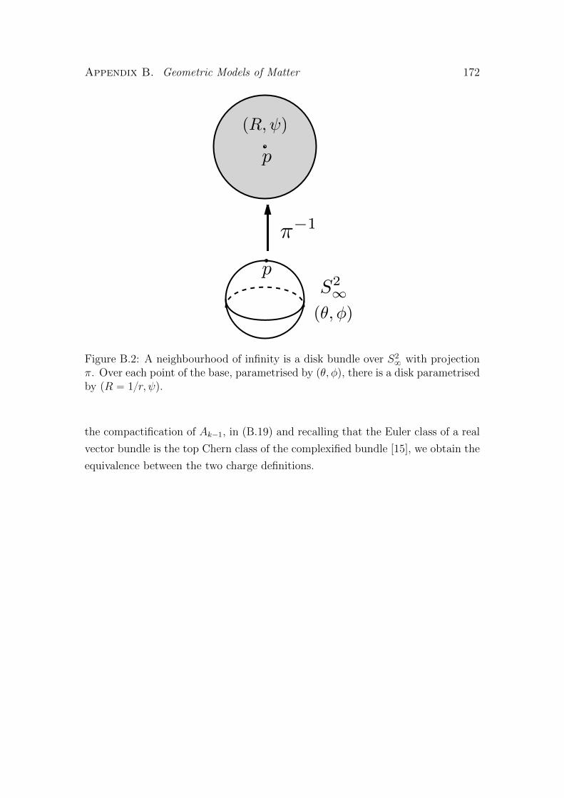
Appendix B. Geometric Models of Matter 172
1
(,)
S2
p
(R,)
p
Figure B.2: A neighbourhood of infinity is a disk bundle over S28 with projection
π. Over each point of the base, parametrised by pθ, φq, there is a disk parametrisedby pR “ 1r, ψq.
the compactification of Ak´1, in (B.19) and recalling that the Euler class of a real
vector bundle is the top Chern class of the complexified bundle [15], we obtain the
equivalence between the two charge definitions.

Appendix B. Geometric Models of Matter 173
B.3 Principal Bundles, Connection and Curva-
ture
This appendix gives a very brief review of connections on principal bundles, mainly
following [64], [65].1
B.3.1 Principal Bundles
Let B be a smooth manifold and G a Lie group. A (smooth) principal G-bundle
P over B is a triple pP, π, σq where P is a smooth manifold, π : P Ñ B a smooth
surjective map and σ : P ˆGÑ P a right action of G on P such that
1. σ preserves the fibres of π:
πpσpu, gqq “ πpuq (B.20)
for all u P P , g P G.
2. P is locally trivial, i.e. for each p0 P B there exists an open neighbourhood
V of p0 in B and a diffeomorphism Ψ : π´1pV q Ñ V ˆ G of the form
Ψpuq “ pπpuq, ψpuqq, with ψ “ π2 ˝ Ψ : π´1pV q Ñ G, where π2 denotes
projection onto the second component, such that
ψpσpu, gqq “ ψpuqg (B.21)
for all u P π´1pV q and g P G.
Note that (B.20) implies
Ψ´1pp, gq “ σ
`
Ψ´1pp, eq, g
˘
(B.22)
for all p P B, g P G, with e the identity element of G. P is called the total space of
the bundle, B the base of the bundle. The pair pV,Ψq is called a local trivialisation.
When there is no danger of confusion we will simply write P for pP, π, σq.
1Note, however, that some signs are different. In particular we use Hermitian rather thananti-Hermitian generators of Lie algebras.

Appendix B. Geometric Models of Matter 174
Let pU,ΨUq, pV,ΨV q be two local trivialisations and consider the quantity
ΨV pΨ´1U pp, gqq “ pp, ψV pΨ
´1U pp, gqqq “ pp, ψV pσpΨ
´1U pp, eq, gqqq
“ pp, ψV pΨ´1U pp, eqq gq “ pp, gV Uppq gq.
(B.23)
The function gV U “ ψV pΨ´1U p¨, eqq : U X V Ñ G is called the transition function
between U and V . Note that gV Uppq can be rewritten as
gV Uppq “ ψV puq pψUpuqq´1, (B.24)
where u is any point in the fibre π´1ppq. In fact
ψV pΨ´1U pp, eqq “ ψV pΨ
´1U pp, ψUpuqpψUpuqq
´1qq “ ψV pσpΨ
´1U pp, ψUpuqq, pψUpuqq
´1qq
“ ψV pΨ´1U pp, ψUpuqqq pψUpuqq
´1“ ψV puq pψUpuqq
´1.
(B.25)
If pP, π, σq, pP 1, π1, σ1q are two principal bundles over the manifolds B and B1,
a map f : P Ñ P 1 is called a principal bundle map provided that σ1 ˝ f “ f ˝ σ.
If B “ B1, a principal bundle map f which is also a diffeomorphism is called an
principal bundle isomorphism. A principal G-bundle over B isomorphic to the
product B ˆG is a trivial principal bundle.
Let pP, π, σq be a principal G-bundle over B and pV,Ψq a trivialising neigh-
bourhood. A local cross-section (shortly, a local section) of P on V is a smooth
map sV : V Ñ π´1pV q such that sV ˝ π “ Id|V . Two local cross-sections sU , sV of
P are related by the equation
sU “ σpsV , gV Uq. (B.26)
If V “ B then sV is a global section. Principal bundles admit global sections if
and only if they are trivial.
Lie groups have a preferred element, the identity, which gives a canonical way
to associate a local section to a local trivialisation. If pV,Ψq is a trivialising neigh-
bourhood, define an associated local section sV by sV ppq “ Ψ´1pp, eq. Conversely,
a local cross-section sV on V determines, since the right action of G on itself is
Appendix B. Geometric Models of Matter 175
free and transitive, a local trivialisation pV,Ψq via ΨpσpsV ppq, gqq “ pp, gq.
B.3.2 Vector Bundles and Associated Vector Bundles
Let B be a smooth manifold, V a vector space. A (smooth) vector bundle E over B
is a pair pE, πq where E is a smooth manifold and π : E Ñ B a smooth surjective
map such that
1. E is locally trivial, i.e. for each p0 P B there exists an open neighbourhood
U of p0 in B and a diffeomorphism Φ : π´1pUq Ñ U ˆ V of the form Φpuq “
pπpuq, φpuqq.
2. For all p P B the map φ|π´1ppq : π´1ppq Ñ V is a vector space isomorphism.
The pair pU,Φq is called a local trivialisation. The rank of E is the dimension of
V .
Let pU,ΦUq, pV,ΦV q be two local trivialisations of a vector bundle E, v P Vand consider the quantity
ΦV pΦ´1U pp, vqq “ pp, φV pΦ
´1U pp, vqqq “ pp, γV Uppq vq. (B.27)
For any fixed p P U X V the function γV Uppq “ φV pΦ´1U pp, ¨qq : V Ñ V is a
vector space isomorphism, therefore γV Uppqmust be an element of GLpk,Rq, where
k “ dimpVq. The map γV U : U XV Ñ GLpk,Rq is the transition function between
U and V . The group GLpk,Rq is called the structure group of V .
If a vector bundle E of rank k has some additional structure then it might be
possible to reduce the structure group G to a subgroup of GLpk,Rq. For example,
if E has a metric then it is always possible to reduce G to Opkq. A vector bundle
is orientable if it is possible to reduce G to GLpk,Rq`, the subgroup of GLpk,Rqconsisting of matrices with positive determinant. The tangent bundle TM of a
manifold M is orientable if and only if M is orientable. The structure group of an
orientable vector bundle endowed with a metric can be reduced to SOpkq.
Let pP, πP , σq be a principal G-bundle over B, V be a vector space and ρ :
GˆV Ñ V a representation of G on V . It is possible to construct a vector bundle
E with base B, fibre V and structure group G, called the vector bundle associated

Appendix B. Geometric Models of Matter 176
to P via ρ (shortly, the associated vector bundle), as follows. The total space is
the quotient
E “ P ˆρ V “P ˆ V„
, (B.28)
where if u, u1 P P , ξ, ξ1 P V , then pu, ξq „ pu1, ξ1q if it exists g P G such that
u “ σpu, gq and ξ “ ρpg´1, ξq. The projection π on P ˆρ V is given by
πpru, ξsq “ πP puq, (B.29)
where ru, ξs denotes an equivalence class in P ˆρ V .
A local trivialisation pU,Ψq of P induces a trivialisation pU,Φq of P ˆρ V , with
Φ given by
Φpru, ξsq “ pπP puq, ρpψpuq, ξq. (B.30)
The inverse is
Φ´1ppp, ξqq “
“
Ψ´1pp, eq, ξ
‰
. (B.31)
If pU,ΨUq, pV,ΨV q are two local trivialisations of P , gUV is the transition function
between V and U on P , pU,ΦUq, pV,ΦV q are the corresponding local trivialisations
on P ˆρ V , then the transition function γUV on P ˆρ V is given by
γUV ppqv “ ρ pgUV ppq, vq . (B.32)
If P is a principal G-bundle, V “ g, ρ “ ad, the associated vector bundle P ˆad g
is called the adjoint bundle and denoted by adP .
B.3.3 Connection Form
Let pP, π, σq be a principal G-bundle over B. A connection form ω : TP Ñ g is a
g-valued 1-form such that, for all W P g, g P G
σ˚gω “ adg´1 ˝ ω, (B.33)
ωpW#q “ W. (B.34)
Here ad : Gˆ gÑ Endpgq is the adjoint representation of G on g and adg : gÑ g
is defined by adgpW q “ adpg,W q. For a matrix Lie group, adgpW q “ gWg´1. The

Appendix B. Geometric Models of Matter 177
map σg : P Ñ P is given by σgpuq “ σpu, gq. The vector field W#, defined by
W#puq “
d
dt
ˇ
ˇ
ˇ
ˇ
t“0
σ`
u, ei tW˘
, (B.35)
is the fundamental vector field on P determined by W P g.
A connection form ω is defined on the total space of the principal bundle P .
Given a local section sV , it is possible to pull ω back to a 1-form locally defined
on the base B of the fibration. The latter is usually called a gauge potential. If sU
and sV are two local cross-sections, the corresponding gauge potentials AU “ s˚Uω
and AV “ s˚V ω are related by the expression
AU “ g´1V U AV gV U ` g´1
V U dgV U , (B.36)
If P is a G-bundle over B and u P P , the vertical subspace VuP of TuP is
defined, without need of any additional structure, as the space tangent to the fibre
at u. However, there is no canonical way of choosing a complement of VuP in
TuP . The required extra structure is given by a connection form ω: the horizontal
subspace HuP of TuP is defined to be the kernel of ωu. For any u P P then
TuP “ HuP ‘ VuP. (B.37)
In fact, by the homomorphism theorem, TuP “ Ker pωuq‘Im pωuq “ HuP‘g. The
spaces g and VuP are isomorphic, an isomorphism being the map W ÞÑ W#puq,
where W P g and W# is the fundamental vector field associated to W . Given
v P TuP , we denote by vH its horizontal part and by vV its vertical part. We say
that v P TuP is vertical if vH “ 0.
Let P be a principal G-bundle, ω a connection on P , α P ΩkpP, gq, the space
of g-valued k-forms on P . The covariant exterior derivative dωα of α is defined
by the equation
dωα pu1, . . . , ukq “ dαppu1qH , . . . , pukqHq, (B.38)
where tuiu are k vector fields on P . If α P ΩkpP, gq then dωα P Ωk`1pP, gq.

Appendix B. Geometric Models of Matter 178
B.3.4 Curvature Form
The curvature form Ω associated to a connection form ω is the g-valued 2-form
Ω “ dωω. (B.39)
An equivalent expression is given by
Ω “ dω ` ω ^ ω. (B.40)
The curvature form Ω satisfies the Bianchi identity
dωΩ “ 0. (B.41)
Note that if G is Abelian then dωω “ dω, the ordinary exterior derivative.
We can obtain 2-forms locally defined on B by pulling back Ω with respect
to local sections of P . If sU : U Ñ P is a local section of P , the field strength
FU P Ω2pU, gq associated to Ω with respect to the local section sU is the pullback
FU “ s˚UΩ. Using (B.40) we see that
FU “ s˚UΩ “ dAU ` AU ^ AU . (B.42)
Note that in (B.40) d is acting on forms defined on P , while in (B.42) it is acting
on forms defined on B.
The transformation property (B.36) of AU induces the following transformation
for FU :
FU “ g´1V U FV gV U . (B.43)
Unless P is trivial or G is Abelian, we can see from (B.43) that there is no globally
defined field strength on B. However if G is Abelian, then FUi “ FUj for any local
sections sUi , sUj of P and we can define a form F P Ω2pB, gq as
F |p “ FU |p (B.44)
where pU,Ψq is any local trivialisation of P such that p P U .
Whether or not G is Abelian it is possible to construct from Ω a globally defined

Appendix B. Geometric Models of Matter 179
2-form FΩ which, however, takes values not in g but in adP . In order to do so we
first we need to give some definitions.
Let V be a vector space, and denote by ΩkpP,Vq, the space of V-valued k-
forms on P . A form α P ΩkpP,Vq is called horizontal if it vanishes when any of
its argument is vertical. If ρ : Gˆ V Ñ V is a representation of G on V , α is said
to be ρ-equivariant if
ρ˚gα “ ρpg´1qα, (B.45)
where ρg “ ρpg, ¨q and ρpg´1qα denotes the action of ρpg´1q on α induced by ρ.
The subspace of ΩkpP,Vq given by horizontal ρ-equivariant k-forms is isomor-
phic to the space ΩkpB,P ˆρ Vq of pP ˆρ Vq-valued k-forms on B, where P ˆρ Vdenotes the vector bundle associated to P [64]. An isomorphism is
α ÞÑ rs, s˚αs, (B.46)
where s is an arbitrary local section of P .
It is evident from (B.41) and the definition of covariant exterior derivative that
Ω is horizontal. It is also ad-equivariant, in fact
σ˚g dω “ d`
σ˚gω˘
“ d padg´1 ˝ ωq “ adg´1 ˝ dω, (B.47)
σ˚g pω ^ ωq “ σ˚gω ^ σ˚gω “ padg´1 ˝ ωq ^ padg´1 ˝ ωq “ adg´1 ˝ pω ^ ωq , (B.48)
so that summing
σ˚gΩ “ adg´1 ˝ Ω. (B.49)
Therefore we can identify Ω with a adP -valued 2-form FΩ on B.
Let sU , sV be two local sections of P . Since FΩ is globally defined on B,
FΩ “ rsU , s˚UΩs “ rsU , FU s
“ rsV , s˚V Ωs “ rsV , FV s “ rσpsU , gUV q, FV s “ rsU , adgUV FV s
“ rsU , gUV FV g´1UV s “ rsU , g
´1V U FV gV U s,
(B.50)
that is FU “ g´1V U FV gV U , which is the transformation law (B.43). Therefore a
collection of field strengths associated to different local trivialisations which are

Appendix B. Geometric Models of Matter 180
related by (B.43), fit together to give a globally defined 2-form FΩ on B, however
such a form takes values on adP rather then g.
If G is Abelian then adg “ Id for all g P G and adP is the trivial vector bundle
B ˆ g. Since field strengths relative to different local trivialisation are equal, we
can write
FΩ “ rs, s˚F s, (B.51)
with F P Ω2pB, gq the globally defined g-valued 2-form on B (B.44). The curvature
form Ω can be written Ω “ π˚PF . In local coordinates one simply has Ω “ FΩ “ F .
B.3.5 Characteristic Classes
In order for the integral over B of a quantity constructed out of FΩ to be well
defined, this quantity needs to be invariant under the transformation (B.43). An
example of invariant quantity is TrpFΩq since TrpFUq “ Trpg´1V U FV gV Uq “ TrpFV q.
More generally, one can consider invariant polynomials in FΩ, i.e. polynomials Psatisfying Ppg´1Wgq “ PpW q for all g P G, W P g. If P is of degree k, then
PpFΩq P Ω2kpB, gq.
Let FΩ, F 1Ω be the adP -valued 2-forms associated to (the curvature of) two
different connections and let P be an invariant polynomial of degree k. It can be
shown that
dPpFΩq “ 0, (B.52)
PpFΩq ´ PpF 1Ωq “ dα, (B.53)
where α P Ω2k´1pB, gq [65]. A consequence of (B.53) is that, provided that B has
no boundary,ż
B
PpFΩq “
ż
B
PpF 1Ωq. (B.54)
A Characteristic class c of a principal bundle P is the cohomology class rPpFΩqs
determined by some particular invariant polynomial P . Because of (B.53), c does
not depend on the chosen connection on P . In fact, characteristic classes measure
topological properties of P . The characteristic class relevant for the electric charge

Appendix B. Geometric Models of Matter 181
definition in chapter 7 is the first Chern class c1pP q, given by2
c1pP q “
„
´1
2πTr pFΩq
. (B.55)
The integral of c1pP q over the base B of P is an integer C1pP q known as the first
Chern number of P .
2Note that we are using Hermitian generators for the Lie algebra.

Appendix B. Geometric Models of Matter 182
B.4 Calculation of R and ||R||2 for Ak´1
In this appendix we compute the curvature 2-form R of Ak´1 working with an
orthonormal coframe, following the standard method described e.g. in [63].
The metric of Ak´1 is
ds2“ V
`
dx2` dy2
` dz2˘
` V ´1pdψ ` αq2 , (B.56)
with
V “ 1`1
2
kÿ
i“1
1
||p´ pi||, (B.57)
an harmonic function. We choose the orthonormal coframe
e1“
1?Vpdψ ` αq ,
e2“?V dx,
e3“?V dy,
e4“?V dz.
(B.58)
The corresponding volume element is
η “ e1^ e2
^ e3^ e4
“ V dψ ^ dx^ dy ^ dz, (B.59)
Since we are working in an orthonormal frame, tensor components with different
indices positioning have the same value.
The connection form ω can be calculated making use of the relations
dei ` ωij ^ ej“ 0. (B.60)

Appendix B. Geometric Models of Matter 183
The result is
ω12 “ ´
1
2V 32
`
BxV e1´ BzV e
3` ByV e
4˘
,
ω13 “ ´
1
2V 32
`
ByV e1` BzV e
2´ BxV e
4˘
,
ω14 “ ´
1
2V 32
`
BzV e1´ ByV e
2` BxV e
3˘
,
ω23 “ ´
1
2V 32
`
BzV e1´ ByV e
2` BxV e
3˘
,
ω24 “ ´
1
2V 32
`
´ByV e1´ BzV e
2` BxV e
4˘
,
ω34 “ ´
1
2V 32
`
BxV e1´ BzV e
3` ByV e
4˘
.
(B.61)
The curvature 2-form R is given by
Rik “ dωik ` ω
ij ^ ω
jk. (B.62)
R is related to the Riemann tensor Rabcd by the relation
Rab “1
2Rabcd e
c^ ed. (B.63)
Since R is self-dual with respect to the orientation (B.59), it satisfies the relations
R12 “ R34, R13 “ ´R24, R14 “ R23. (B.64)
Self duality of R and the symmetry Rabcd “ Rcdab of the Riemann tensor imply
that each of the 2-forms Rab is self-dual, that is
pRabq12 “ pRabq34 , pRabq13 “ ´pRabq24 , pRabq14 “ pRabq23 . (B.65)

Appendix B. Geometric Models of Matter 184
The result is
R12 “ R34 “1
2V 3
`
V BxxV ´ 2pBxV q2` pByV q
2` pBzV q
2˘ `
e1^ e2
` e3^ e4
˘
`1
2V 3pV BxyV ´ 3BxV ByV q
`
e1^ e3
´ e2^ e4
˘
`1
2V 3pV BxzV ´ 3BxV BzV q
`
e1^ e4
` e2^ e3
˘
,
R13 “ R42 “1
2V 3pV BxyV ´ 3BxV ByV q
`
e1^ e2
` e3^ e4
˘
`1
2V 3
`
V ByyV ´ 2pByV q2` pBxV q
2` pBzV q
2˘ `
e1^ e3
´ e2^ e4
˘
`1
2V 3pV ByzV ´ 3ByV BzV q
`
e1^ e4
` e2^ e3
˘
,
R14 “ R23 “1
2V 3pV BxzV ´ 3BxV BzV q
`
e1^ e2
` e3^ e4
˘
`1
2V 3pV ByzV ´ 3ByV BzV q
`
e1^ e3
´ e2^ e4
˘
`1
2V 3
`
V BzzV ´ 2pBzV q2` pBxV q
2` pByV q
2˘ `
e1^ e4
` e2^ e3
˘
.
(B.66)
The squared L2-norm ||R||2 of R is given by
||R||2 η “ 1
2R^ ˚R “ 1
2R^R “
4ÿ
aăb“1
Rab ^Rab
“ 2 pR12 ^R12 `R13 ^R13 `R14 ^R14q
“ 24ÿ
aăb“1
´
pR12abq2` pR13abq
2` pR14abq
2¯
η
“ 4”
pR1212q2` pR1313q
2` pR1414q
2` 2
`
pR1213q2` pR1214q
2` pR1314q
2˘
ı
η.
(B.67)

Appendix B. Geometric Models of Matter 185
Substituting (B.66) gives
||R||2 “ 1
V 4
´
pBxxV q2` pByyV q
2` pBzzV q
2` 2pBxyV q
2` 2pByzV q
2` 2pBzxV q
2¯
`6
V 5
´
pBxV q2BxxV ` pByV q
2ByyV ` pBzV q
2BzzV
´ 2BxV ByV BxyV ´ 2ByV BzV ByzV ´ 2BzV BxV BzxV¯
`6
V 6
´
pBxV q2` pByV q
2` pBxV q
2¯2
.
(B.68)
Integral of ||R||2 η over A0
On A0 is more convenient to use the coordinates (r, θ, φ, ψ) (7.37) in terms of
which V “ 1` 1p2rq and
ds2“ V pdr2
` r2dΩ2q ` V ´1
ˆ
dψ `1
2cos θ dφ
˙2
. (B.69)
We choose the orthonormal coframe
ε1 “1?V
ˆ
dψ `1
2cos θ dφ
˙
,
ε2 “?V dr,
ε3 “?V r dθ,
ε4 “?V r sin θ dφ.
(B.70)
The corresponding volume element is
η “ ε1 ^ ε2 ^ ε3 ^ ε4 “ r2V sin θ dψ ^ dr ^ dθ ^ dφ. (B.71)
The bases (B.58) and (B.70) are related by the transformation ea1
“ Λa1
a εa,
where
Λ “
¨
˚
˚
˚
˚
˝
1 0 0 0
0 sin θ cosφ cos θ cosφ ´ sinφ
0 sin θ sinφ cos θ sinφ cosφ
0 cos θ ´ sin θ 0
˛
‹
‹
‹
‹
‚
. (B.72)

Appendix B. Geometric Models of Matter 186
Since, denoting with unprimed (primed) indices the components of R with respect
to the basis tεau (tea1
u),
Rab “ Rab “
`
Λ´1˘a
a1Ra1
b1 Λb1
b, (B.73)
we have
R12 “ R34 “4
p1` 2rq3`
ε1 ^ ε2 ` ε3 ^ ε4˘
,
R13 “ R42 “ ´2
p1` 2rq3`
ε1 ^ ε3 ´ ε2 ^ ε4˘
,
R14 “ R23 “ ´2
p1` 2rq3`
ε1 ^ ε4 ` ε2 ^ ε3˘
.
(B.74)
The squared L2-norm of R is
||R||2 “ 96
p1` 2rq6. (B.75)
The integral of ||R||2 η over A0 is
ż
A0
||R||2 η “ż 2π
0
dφ
ż 2π
0
dψ
ż π
0
sin θ dθ
ż 8
0
96
p1` 2rq6r2
ˆ
1`1
2r
˙
dr
“ 8π2
ż 8
0
48r
p1` 2rq5dr “ 8π2,
(B.76)
having used (8.28).
Direct integration of ||R||2 η over Ak´1 is not a viable if k ą 2, so let us repeat
the calculation using a different method which can be applied for any value of k.
Write
||R||2 η “ ´ 48r
p1` 2rq5sin θ dr ^ dψ ^ dθ ^ dφ
“ d
ˆ
1` 8r
p1` 2rq4sin θ ` fpθ, φ, ψq
˙
^ dψ ^ dθ ^ dφ
“ d
„ˆ
1` 8r
p1` 2rq4sin θ ` fpθ, φ, ψq
˙
dψ ^ dθ ^ dφ
“ dY ,
(B.77)

Appendix B. Geometric Models of Matter 187
where f is an arbitrary function of the angular variables, and
Y “ˆ
1` 8r
p1` 2rq4sin θ ` fpθ, φ, ψq
˙
dψ ^ dθ ^ dφ. (B.78)
Having written ||R||2 η as a total derivative, we can calculate its integral over A0
using Stokes’ theorem. However in order to do so, Y needs to be well-defined on
the whole of A0. Since the angular coordinates are ill-defined for r “ 0, we need
to take fpθ, φ, ψq “ ´ sin θ.
The 3-form Y is not compactly supported so, proceeding in a similar way as
we did when calculating the integral (8.24) in chapter 8, we first restrict it to the
compact manifold with boundary
AR0 “ tu P A0 | ||πA0puq|| ď Ru, (B.79)
where R " 1 and πA0 is the projection from A0 to R3 mapping each circle to its
base-point, apply Stokes’ theorem and finally take the limit for RÑ 8:
ż
A0
||R||2 η “ limRÑ8
ż
AR0
d pY dψ ^ dθ ^ dφq “ limRÑ8
ż
BAR0
Y dψ ^ dθ ^ dφ
“ ´8π2 limRÑ8
ˆ
1` 8R
p1` 2Rq4´ 1
˙
“ 8π2,
(B.80)
having used (8.28).
Integral of ||R||2 η over Ak´1
Since H2pAk´1q “ 0, we know that ||R||2 η is exact. Let us try to write its primitive
as
||R||2 η “ ||R||2 r2V sin θ dψ ^ dr ^ dθ ^ dφ
“ Y dr ^ dψ ^ dθ ^ dφ “ dY ^ dψ ^ dθ ^ dφ
“ d pY dψ ^ dθ ^ dφq ,
(B.81)

Appendix B. Geometric Models of Matter 188
where
Y “ ´ ||R||2 V r2 sin θ,
Y “ż
Y pr, θ, φq dr.(B.82)
Clearly Y is determined up to an arbitrary function fpθ, φ, ψq which we will de-
termine imposing that the Y is well defined on Ak´1. Restricting the integral to
the compact manifold with boundary
ARk´1 “ tu P Ak´1 |ˇ
ˇ
ˇ
ˇπAk´1puq
ˇ
ˇ
ˇ
ˇ ď Ru, (B.83)
where R " ||pi|| for all i, we have
ż
Ak´1
||R||2 η “ limRÑ8
ż
ARk´1
d pY dψ ^ dθ ^ dφq “ limRÑ8
ż
BARk´1
Y dψ ^ dθ ^ dφ.
(B.84)
Y is a complicated function of r, θ, φ, ψ but we can easily estimate its large r
behaviour up to OpR´1q corrections which vanish in the limit RÑ 8. At large r,
V „ 1` kp2rq and (B.68) reduces to 96k2pk ` 2rq6, so asymptotically
Y “ ´48k2r
pk ` 2rq5sin θ dr ^ dψ ^ dθ ^ dφ,
Y “ˆ
k2 k ` 8r
pk ` 2rq4sin θ ` fpθ, φ, ψq
˙
dψ ^ dθ ^ dφ.
(B.85)
Since (B.85) is only valid asymptotically, we need to check that Y is well-defined
not at r “ 0, but at the NUTs positions. Near a NUT pi, up to corrections
vanishing in the r Ñ pi limit, Y is given by (B.78) but with spherical coordinates
centred at pi,
Y “ˆ
´1` 8 ||p´ pi||
p1` 2 ||p´ pi||q4sin θi ` fpθ, φ, ψq
˙
dψ ^ dθ ^ dφ, (B.86)
where θi “ arccosppz ´ ziq ||p´ pi||q. The 3-form (B.86) is ill-defined at p “ pi
unless fpθ, φ, ψq “ ´ sin θi. Therefore we need to take, summing over all the

Appendix B. Geometric Models of Matter 189
NUTs,
f “ ´kÿ
i“1
sin θi. (B.87)
Asymptotically f “ ´k sin θ, therefore
ż
Ak´1
||R||2 η “ k limRÑ8
ż
BARk´1
ˆ
kk ` 8r
pk ` 2rq4´ 1
˙
sin θ dψ ^ dθ ^ dφ
“ ´8π2k limRÑ8
ˆ
kk ` 8R
pk ` 2Rq4´ 1
˙
“ 8π2 k.
(B.88)

Bibliography
[1] A. Amo, J. Lefrere, S. Pigeon, C. Adrados, C. Ciuti, I. Carusotto, R. Houdre,
E. Giacobino, and A. Bramati. Superfluidity of polaritons in semiconductor
microcavities. Nature Phys., 5:805–810, 2009.
[2] A. Amo, S. Pigeon, D. Sanvitto, V. G. Sala, R. Hivet, I. Carusotto,
F. Pisanello, G. Lemenager, R. Houdre, E. Giacobino, C. Ciuti, and A. Bra-
mati. Polariton superfluids reveal quantum hydrodynamic solitons. Science,
332:1167–1170, 2011.
[3] I. Aranson and L. Kramer. The world of the complex Ginzburg-Landau equa-
tion. Rev. Mod. Phys., 74:99–143, 2002.
[4] F. Arecchi, S. Boccaletti, and P. Ramazza. Pattern formation and competition
in nonlinear optics. Phys. Rep., 318:1–83, 1999.
[5] M. Atiyah and N. J. Hitchin. The geometry and dynamics of magnetic
monopoles. Princeton University Press, 1988.
[6] M. Atiyah, N. S. Manton, and B. J. Schroers. Geometric models of matter.
Proc. R. Soc. Lond. A, 468:1–28, 2012.
[7] O. Avenel, P. Hakonen, and E. Varoquaux. Detection of the rotation of the
Earth with a superfluid gyrometer. Phys. Rev. Lett., 78:3602–3605, 1997.
[8] V. Bagnato and D. Kleppner. Bose-Einstein condensation in low-dimensional
traps. Phys. Rev. A, 44:7439–7441, 1991.
[9] D. Bajoni, P. Senellart, E. Wertz, I. Sagnes, A. Miard, A. Lemaıtre, and
J. Bloch. Polariton laser using single micropillar GaAs-GaAlAs semiconductor
cavities. Phys. Rev. Lett., 100:047401, 2008.
190

BIBLIOGRAPHY 191
[10] R. B. Balili, V. Hartwell, D. W. Snoke, L. Pfeiffer, and K. West. Bose-Einstein
condensation of microcavity polaritons in a trap. Science, 316:1007–1010,
2007.
[11] V. L. Berezinskii. Destruction of long-range order in one-dimensional and
two-dimensional systems having a continuous symmetry group ii Quantum
systems. Sov. Phys. JETP, 34:610–616, 1972.
[12] A. L. Besse. Einstein manifolds. Springer, 1987.
[13] O. Biquard and V. Minerbe. A Kummer construction for gravitational in-
stantons. Commun. Math. Phys., 308:1–24, 2011.
[14] M. Borgh, G. Franchetti, J. M. J. Keeling, and N. G. Berloff. Robustness and
observability of rotating vortex lattices in an exciton-polariton condensate.
Phys. Rev. B, 86:035307, 2012.
[15] R. Bott and L. W. Tu. Differential forms in algebraic topology. Springer,
1982.
[16] V. A. Brazhnyi and V. V. Konotop. Theory of nonlinear matter waves in
optical lattices. Modern Phys. Lett. B, 18:627–551, 2004.
[17] L. V. Butov and A. V. Kavokin. The behaviour of exciton-polaritons. Nature
Photon., 6, 2012.
[18] G. Chalmers, M. Rocek, and S. Wiles. Degeneration of ALF Dn metrics. J.
High Energy Phys., 01:009, 1999.
[19] S. Cherkis. Self-dual gravitational instantons. Talk given at the AIM workshop
“L2-cohomology in geometry and physics”, Palo Alto, USA, 2004.
[20] S. Cherkis. Doubly-periodic monopoles and their moduli spaces. Talk given
at the BIRS workshop “Advances in hyperkahler and holomorphic symplectic
geometry”, Nanff, Canada, 2012.
[21] S. A. Cherkis and N. J. Hitchin. Gravitational instantons of type Dk. Com-
mun. Math. Phys., 260:299–317, 2005.

BIBLIOGRAPHY 192
[22] S. A. Cherkis and A. Kapustin. Singular monopoles and supersymmetric
gauge theories in three dimensions. Nucl. Phys. B, 525:713–728, 1998.
[23] S. A. Cherkis and A. Kapustin. Singular monopoles and gravitational instan-
tons. Commun. Math. Phys., 203:215–234, 1999.
[24] G. Christmann, G. Tosi, N. G. Berloff, P. Tsotsis, P. S. Eldridge, Z. Hat-
zopoulos, P. G. Savvidis, and J. J. Baumberg. Polariton ring condensates and
sunflower ripples in an expanding quantum liquid. Phys. Rev. B, 85:235303,
2012.
[25] S. Coleman. There are no Goldstone bosons in two dimensions. Commun.
Math. Phys., 31:259–264, 1973.
[26] P. Cristofolini, A. Dreismann, G. Christmann, G. Franchetti, N. G. Berloff,
P. Tsotsis, Z. Hatzopoulos, P. G. Savvidis, and J. J. Baumberg. Optical
superfluid phase transitions and trapping of polariton condensates. Phys.
Rev. Lett., 110:186403, 2013.
[27] A. S. Dancer. A family of hyperkahler manifolds. Quart. J. Math. Oxford,
45:463–478, 1994.
[28] G. Dasbach, M. Schwab, M. Bayer, and A. Forchel. Parametric polariton scat-
tering in microresonators with three-dimensional optical confinement. Phys.
Rev. B, 64:201309, 2001.
[29] M. P. do Carmo. Differential geometry of curves and surfaces. Prentice-Hall,
1976.
[30] T. D. Doan, H. T. Cao, D. B. Tran Thoai, and H. Haug. Microcavity polariton
kinetics for bosonic condensation and lasing in ii-vi compound materials. Phys.
Rev. B, 74:15316, 2006.
[31] T. D. Doan and D. B. Tran Thoai. Suppression of the bottleneck in semicon-
ductor microcavities. Solid State Commun., 123:427–430, 2002.
[32] M. Dunajski. Solitons, Instantons, and Twistors. Oxford University Press,
2010.

BIBLIOGRAPHY 193
[33] G. Etesi. The topology of asymptotically locally flat gravitational instantons.
Phys. Lett. B, 641:461–465, 2006.
[34] L. Ferrier, E. Wertz, R. Johne, D. D. Solnyshkov, P. Senellart, I. Sagnes,
A. Lemaıtre, G. Malpuech, and J. Bloch. Interactions in confined polariton
condensates. Phys. Rev. Lett., 106:126401, 2011.
[35] G. Franchetti, N. G. Berloff, and J. J. Baumberg. Exploiting quantum coher-
ence of polaritons for ultra sensitive detectors, 2012, arXiv:1210.1187v2.
[36] G. Franchetti and N. S. Manton. Gravitational instantons as models for
charged particle systems. J. High Energy Phys., 03:072, 2013.
[37] G. Gibbons and S. W. Hawking. Gravitational multi-instantons. Phys. Lett.
B, 78:430–432, 1978.
[38] G. Gibbons and S. W. Hawking. Classification of gravitational instanton
symmetries. Commun. Math. Phys., 66:291–310, 1979.
[39] G. Gibbons and N. S. Manton. Classical and quantum dynamics of BPS
monopoles. Nucl. Phys. B, 274:183–224, 1986.
[40] G. Gibbons, C. Pope, and H. Romer. Index theorem boundary terms for
gravitational instantons. Nucl. Phys. B, 157:377–386, 1979.
[41] P. B. Gilkey. The boundary integrand in the formula for the signature and
Euler characteristic of a Riemannian manifold with boundary. Adv. Math.,
15:334–360, 1975.
[42] D. J. Gross and M. J. Perry. Magnetic monopoles in Kaluza-Klein theories.
Nucl. Phys. B, 226:29–48, 1983.
[43] V. Guillemin and A. Pollack. Differential topology. AMS Chelsea Publishing,
2010.
[44] P. S. Hagan. Spiral waves in reaction-diffusion equations. SIAM J. Appl.
Math, 42:762–786, 1982.

BIBLIOGRAPHY 194
[45] T. Hausel, E. Hunsicker, and R. Mazzeo. Hodge cohomology of gravitational
instantons. Duke Math. J., 122:153–165, 2004.
[46] S. W. Hawking. Gravitational instantons. Phys. Lett. A, 60:81–83, 1977.
[47] N. J. Hitchin. Twistor construction of Einstein metrics. In Global Riemannian
geometry (Durham, 1983), Ellis Horwood Ser. Math. Ellis Horwood, 1984.
[48] K. Huang. Statistical Mechanics. John Wiley & Sons, 1987.
[49] R. I. Kaitouni, O. El Daıf, A. Baas, M. Richard, T. Paraiso, P. Lugan, T. Guil-
let, F. Morier-Genoud, J. Ganiere, J. Staehli, V. Savona, and B. Deveaud.
Engineering the spatial confinement of exciton polaritons in semiconductors.
Phys. Rev. B, 74:155311, 2006.
[50] T. Kaluza. Zum unitatsproblem der physik. Sitz. Preuss. Akad. Wiss. Phys.
Math. K, 1:966–972, 1921.
[51] J. Kasprzak, M. Richard, S. Kundermann, A. Baas, P. Jeambrun, J. M. J.
Keeling, F. Marchetti, M. H. Szymanska, R. Andre, J. L. Staehli, V. Savona,
P. B. Littlewood, B. Deveaud, and L. S. Dang. Bose-Einstein condensation
of exciton polaritons. Nature, 443:409–414, 2006.
[52] J. M. J. Keeling and N. G. Berloff. Spontaneous rotating vortex lattices in a
pumped decaying condensate. Phys. Rev. Lett., 100:250401, 2008.
[53] J. M. J. Keeling and N. G. Berloff. Exciton–polariton condensation. Contemp.
Phys., 52:131–151, 2011.
[54] O. Klein. Quantentheorie und funfdimensionale relativitatstheorie. Zeits.
Phys., 37:895–906, 1926.
[55] J. M. Kosterlitz and D. J. Thouless. Ordering, metastability and phase tran-
sitions in two-dimensional systems. J. Phys. C, 6:1181–1203, 1973.
[56] B. P. Kronheimer. The construction of ALE spaces as hyper-Kahler quotients.
J. Differ. Geom., 29:665–683, 1989.

BIBLIOGRAPHY 195
[57] J. Lega and S. Fauve. Traveling hole solutions to the complex Ginzburg-
Landau equation as perturbations of nonlinear Schrodinger dark solitons.
Physica D, 102:234–252, 1997.
[58] G. Malpuech, Y. G. Rubo, F. P. Laussy, P. Bigenwald, and A. V. Kavokin.
Polariton laser: thermodynamics and quantum kinetic theory. Semicond. Sci.
Technol., 18:S 395, 2003.
[59] N. Manton and P. Sutcliffe. Topological Solitons. Cambridge University Press,
2004.
[60] N. D. Mermin and H. Wagner. Absence of ferromagnetism or antiferromag-
netism in one- or two-dimensional isotropic Heisenberg models. Phys. Rev.
Lett., 17:1307, 1966.
[61] V. Minerbe. On the asymptotic geometry of gravitational instantons. Ann.
Sci. Ec. Norm. Sup., 43:1–39, 2010.
[62] C. W. Misner. The flatter regions of Newman, Unti, and Tamburino’s gener-
alized Schwarzschild space. J. Math. Phys., 4:924–937, 1963.
[63] C. W. Misner, K. S. Thorne, and J. A. Wheeler. Gravitation. W. H. Freeman,
1973.
[64] G. L. Naber. Topology, geometry and gauge fields, volume 1. Springer, 2010.
[65] G. L. Naber. Topology, geometry and gauge fields, volume 2. Springer, 2010.
[66] M. Nakahara. Geometry, Topology and Physics. Taylor & Francis, 2003.
[67] B. Nelsen, G. Liu, M. Steger, D. Snoke, R. Balili, K. West, and L. Pfeiffer.
Coherent flow and trapping of polariton condensates with long lifetime, 2012,
arXiv:1209.4573.
[68] J. C. Neu. Vortices in complex scalar fields. Physica D, 43:385–406, 1990.
[69] L. Nicolaescu. Intersection theory, 2011, http://www3.nd.edu/~lnicolae/
TopicsFall2011-Intersect.pdf.

BIBLIOGRAPHY 196
[70] J. M. Overduin and P. S. Wesson. Kaluza-Klein gravity. Phys. Rep., 283:303–
378, 1997.
[71] R. Packard and S. Vitale. Principles of superfluid-helium gyroscopes. Phys.
Rev. B, 46:3540–3549, 1992.
[72] L. M. Pismen. Vortices in Nonlinear Fields. Oxford University Press, 1999.
[73] L. M. Pismen and A. A. Nepomnyashchy. On interaction of spiral waves.
Physica D, 54:183–193, 1992.
[74] L. Pitaevskii and S. Stringari. Bose-Einstein Condensation. Clarendon Press,
2003.
[75] A. Posazhennikova. Colloquium: weakly interacting, dilute Bose gases in 2D.
Rev. Mod. Phys., 78:1111–1134, 2006.
[76] P. H. Roberts and N. G. Berloff. The nonlinear Schrodinger equation as a
model of superfluidity. In C. F. Barenghi, R. J. Donnelly, and W. F. Vinen, ed-
itors, Quantized Vortex Dynamics and Superfluid Turbulence. Springer, 2001.
[77] D. S. Rokhsar. Vortex stability and persistent currents in trapped Bose gases.
Phys. Rev. Lett., 79:2164–2167, 1997.
[78] P. Ruback. The motion of Kaluza-Klein monopoles. Commun. Math. Phys.,
107:93–102, 1986.
[79] V. Savona. Effect of interface disorder on quantum well excitons and micro-
cavity polaritons. J. Phys.: Condens. Matt., 19:295208, 2007.
[80] A. Scorpan. The Wild World of 4-Manifolds. American Mathematical Society,
2005.
[81] A. Sen. A note on enhanced gauge symmetries in M- and string theory. J.
High Energy Phys., 09:001, 1997.
[82] I. A. Shelykh, A. V. Kavokin, Y. G. Rubo, T. C. H. Liew, and G. Malpuech.
Polariton polarization-sensitive phenomena in planar semiconductor micro-
cavities. Semicond. Sci. Technol., 25:013001, 2010.

BIBLIOGRAPHY 197
[83] M. Sich, D. N. Krizhanovskii, M. S. Skolnick, A. V. Gorbach, R. Hartley,
D. V. Skryabin, E. A. Cerda-Mendez, K. Biermann, R. Hey, and P. V. San-
tos. Observation of bright polariton solitons in a semiconductor microcavity.
Nature Photon., 6:50–55, 2011.
[84] K. Staliunas and V. J. Sanchez-Morcillo. Transverse Patterns in Nonlinear
Optical Resonators. Springer, 2003.
[85] G. Tosi, G. Christmann, N. G. Berloff, P. Tsotsis, T. Gao, Z. Hatzopoulos,
P. G. Savvidis, and J. J. Baumberg. Sculpting oscillators with light within a
nonlinear quantum fluid. Nature Phys., 8:190–194, 2012.
[86] R. M. Wald. General Relativity. University of Chicago Press, 1984.
[87] E. Wertz, L. Ferrier, D. D. Solnyshkov, R. Johne, D. Sanvitto, A. Lemaıtre,
I. Sagnes, R. Grousson, A. V. Kavokin, P. Senellart, G. Malpuech, and
J. Bloch. Spontaneous formation and optical manipulation of extended po-
lariton condensates. Nature Phys., 6:860–864, 2010.
[88] M. Wouters and I. Carusotto. Excitations in a nonequilibrium Bose-Einstein
condensate of exciton polaritons. Phys. Rev. Lett., 99:140402, 2007.
[89] M. Wouters and I. Carusotto. Superfluidity and critical velocities in nonequi-
librium Bose-Einstein condensates. Phys. Rev. Lett., 105:020602, 2010.
[90] M. Wouters, T. C. H. Liew, and V. Savona. Energy relaxation in one-
dimensional polariton condensates. Phys. Rev. B, 82:245315, 2010.