PATTERN FORMATION IN COUPLED

NETWORKS WITH INHIBITION AND GAP

JUNCTIONS

by

Fatma Gurel Kazancı

B.S. Mathematics, Middle East Technical University, 2000

Submitted to the Graduate Faculty of

the School of Arts and Sciences in partial fulfillment

of the requirements for the degree of

Doctor of Philosophy

University of Pittsburgh

2007

UNIVERSITY OF PITTSBURGH

SCHOOL OF ARTS AND SCIENCES

This dissertation was presented

by

Fatma Gurel Kazancı

It was defended on

January 30

and approved by

G. Bard Ermentrout, Department of Mathematics

Jonathan Rubin, Department of Mathematics

William Troy, Department of Mathematics

Nathan Urban, Department of Biological Sciences, CMU

Dissertation Director: G. Bard Ermentrout, Department of Mathematics

ii

PATTERN FORMATION IN COUPLED NETWORKS WITH INHIBITION

AND GAP JUNCTIONS

Fatma Gurel Kazancı, PhD

University of Pittsburgh, 2007

G. Bard Ermentrout, Dissertation Director

In this dissertation we analyze networks of coupled phase oscillators. We consider systems

where long range chemical coupling and short range electrical coupling have opposite effects

on the synchronization process. We look at the existence and stability of three patterns of

activity: synchrony, clustered state and asynchrony.

In Chapter 1, we develop a minimal phase model using experimental results for the

olfactory system of Limax. We study the synchronous solution as the strength of synaptic

coupling increases. We explain the emergence of traveling waves in the system without a

frequency gradient. We construct the normal form for the pitchfork bifurcation and compare

our analytical results with numerical simulations.

In Chapter 2, we study a mean-field coupled network of phase oscillators for which a

stable two-cluster solution exists. The addition of nearest neighbor gap junction coupling

destroys the stability of the cluster solution. When the gap junction coupling is strong

there is a series of traveling wave solutions depending on the size of the network. We see

bistability in the system between clustered state, periodic solutions and traveling waves. The

iii

bistability properties also change with the network size. We analyze the system numerically

and analytically.

In Chapter 3, we turn our attention to a very popular model about network synchroniza-

tion. We represent the Kuramoto model in its original form and calculate the main results

using a different technique. We also look at a modified version and study how this effects

synchronization. We consider a collection of oscillators organized in m groups. The addition

of gap junctions creates a wave like behavior.

iv

TABLE OF CONTENTS

PREFACE . . . . . . . . . . . . . . . . . . . . . . . . . . . . . . . . . . . . . . . . . ix

1.0 INTRODUCTION . . . . . . . . . . . . . . . . . . . . . . . . . . . . . . . . . 1

2.0 SYNCHRONY AND TRAVELING WAVES . . . . . . . . . . . . . . . . 5

2.1 Introduction . . . . . . . . . . . . . . . . . . . . . . . . . . . . . . . . . . . 5

2.2 Motivation: Limax Model . . . . . . . . . . . . . . . . . . . . . . . . . . . 7

2.3 The Biophysical Model and Reduction . . . . . . . . . . . . . . . . . . . . 10

2.3.1 The spatial equations . . . . . . . . . . . . . . . . . . . . . . . . . . 15

2.4 Linear Stability Analysis for Synchronous Solution . . . . . . . . . . . . . . 17

2.5 Existence and Stability of the Traveling Wave . . . . . . . . . . . . . . . . 23

2.6 Numerical Results . . . . . . . . . . . . . . . . . . . . . . . . . . . . . . . 26

2.7 Conclusions . . . . . . . . . . . . . . . . . . . . . . . . . . . . . . . . . . . 32

3.0 CLUSTERING IN COUPLED NEURAL OSCILLATORS . . . . . . . . 35

3.1 Introduction . . . . . . . . . . . . . . . . . . . . . . . . . . . . . . . . . . . 35

3.2 The Base Model . . . . . . . . . . . . . . . . . . . . . . . . . . . . . . . . . 37

3.2.1 Application . . . . . . . . . . . . . . . . . . . . . . . . . . . . . . . . 42

3.3 The Full Model with Gap Junctions . . . . . . . . . . . . . . . . . . . . . . 46

3.4 Numerical Results . . . . . . . . . . . . . . . . . . . . . . . . . . . . . . . 47

v

3.5 Conclusions . . . . . . . . . . . . . . . . . . . . . . . . . . . . . . . . . . . 53

4.0 ASYNCHRONY . . . . . . . . . . . . . . . . . . . . . . . . . . . . . . . . . . 58

4.1 Introduction . . . . . . . . . . . . . . . . . . . . . . . . . . . . . . . . . . . 58

4.2 The Kuramoto Model . . . . . . . . . . . . . . . . . . . . . . . . . . . . . . 59

4.3 Kuramoto Model with Gap Junctions . . . . . . . . . . . . . . . . . . . . . 66

4.4 Conclusions . . . . . . . . . . . . . . . . . . . . . . . . . . . . . . . . . . . 71

5.0 DISCUSSION . . . . . . . . . . . . . . . . . . . . . . . . . . . . . . . . . . . . 72

APPENDIX A. PHASE MODEL REDUCTION . . . . . . . . . . . . . . . . . 74

A.1 Phase Model and Averaging . . . . . . . . . . . . . . . . . . . . . . . . . . 74

A.2 Biophysical Model and Coupling Functions . . . . . . . . . . . . . . . . . . 77

APPENDIX B. NORMAL FORM CALCULATION . . . . . . . . . . . . . . 79

BIBLIOGRAPHY . . . . . . . . . . . . . . . . . . . . . . . . . . . . . . . . . . . . 84

vi

LIST OF FIGURES

2.2.1 Oscillatory behavior of the neurons . . . . . . . . . . . . . . . . . . . . . . . 9

2.3.1 Coupling functions computed using XPPAUT . . . . . . . . . . . . . . . . . 13

2.3.2 A plot of J(x) . . . . . . . . . . . . . . . . . . . . . . . . . . . . . . . . . . . 18

2.6.1 Transition from synchrony to traveling wave. . . . . . . . . . . . . . . . . . . 28

2.6.2 Evolution of the solution to the discrete phase model . . . . . . . . . . . . . 30

2.6.3 Behavior of the conductance-based model . . . . . . . . . . . . . . . . . . . 31

2.6.4 Behavior of 20 phase oscillators in a line . . . . . . . . . . . . . . . . . . . . 33

3.2.1 Possible values for p are graphed as φ varies from 0 to 2π . . . . . . . . . . . 43

3.2.2 Eigenvalues for the system in 3.5 . . . . . . . . . . . . . . . . . . . . . . . . 45

3.3.1 Relation between ggap and N . . . . . . . . . . . . . . . . . . . . . . . . . . 48

3.4.1 Two-cluster solution . . . . . . . . . . . . . . . . . . . . . . . . . . . . . . . 49

3.4.2 Bifurcation diagram for parameter ggap . . . . . . . . . . . . . . . . . . . . . 51

3.4.3 Bifurcation diagrams for various N values . . . . . . . . . . . . . . . . . . . 52

3.4.4 Traveling waves and other patterns with 10 oscillators. . . . . . . . . . . . . 54

3.4.5 Periodic orbits close to homoclinic . . . . . . . . . . . . . . . . . . . . . . . 55

3.4.6 Double traveling wave and double zig-zag patterns . . . . . . . . . . . . . . 56

4.1.1 Illustrative figure of a collection of oscillators . . . . . . . . . . . . . . . . . 60

vii

4.3.1 Asynchronous solution with gap junctions . . . . . . . . . . . . . . . . . . . 70

viii

PREFACE

I would like to thank the members of my thesis committee, Prof. Troy, Prof. Rubin and

Prof. Urban. I learned a great deal from Prof. Troy and Prof. Rubin during the classes I

have taken with them. Their contribution to my education process is invaluable.

I also thank Prof. Riviere, Prof. Hastings, Prof. Yotov and Prof. Lennard for their

guidance throughout the years. It is an honor to be a student in any of your classes. My

special thanks also goes to Ms. Cathy Duane-Lennard, I was honored to work with you.

I am in debt to my Ph.D advisor, Prof. Bard Ermentrout for everything I have learned

from him. I wish that this process never ends and hopefully we continue collaborating in

the future. I will miss his teaching style, jokes and more than ever his never ending energy

and hunger for science. I thank him for introducing to me to this field and for supporting

me during my education in many ways.

I would also like to thank the wonderful staff of the Math Department, especially Drew

Porvaznik and Molly Williams for helping me with all the little details along my studentship.

I thank all my student friends at Pitt. Special thanks goes to Monika and Alfy (survivors

from class of 2001); fellow fifth floor residents Angela, Jyotsna, Carolina and Evandro for the

lovely conversations and their friendship; ex-Pitt students Lerna, Atife, Songul, Huseyin and

Meryem for the comfort of conversing in Turkish and good food; and my dear officemates:

ix

Stephanie, Aushra and Jon for maintaining a peaceful study environment and for their

friendship. Thanks for all the good times. You will be missed greatly.

I would like to extend my many thanks to my family, my mom, dad, brothers, sisters,

nieces, nephews, extended family and my friends both from Pittsburgh and Turkey. Your

love, support and prayers keeps me going. Last but not least, I would like to thank my

husband, Caner, for always supporting me, helping me whenever I needed help and always

being there for me. I couldn’t have done it without you.

I would like to dedicate my thesis to the memory of my grandfather Mashar Erol who

passed away in 2000. He would have been very happy to see this day.

x

1.0 INTRODUCTION

Study of the human brain has been the interest of researchers for centuries. The anatomy

of human brain is fairly well-known. This vast complex contains more than one hundred

billion neurons which are connected to other neurons via electrical and/or chemical synapses.

Advances in experimental methods and imaging techniques enabled researchers to learn the

architecture in different areas of the brain. However, there is still a long way to go before

we fully understand how the brain functions and generates various rhythms. Collaboration

among scientists from both experimental and theoretical backgrounds is needed to solve

this big puzzle. Mathematical modeling is useful in combining the physiological information

and neural function. Models developed for specific areas help us gain insight into how that

particular part works and hopefully leads us to theories that are applicable to similar systems.

For computational purposes, neurons can be considered as intrinsic oscillators. Each

neuron is coupled to others via electrical and/or chemical synapses. Often times when we

try to model a system, we have limited information about the parameters. We also want to

make a model that is small enough so that we can perform efficient numerical simulations

or mathematically analyze it but large enough to capture the important features of the

system. We will use phase models to represent the systems we study. These models can be

used to explain biophysical data showing synchronization in areas of brain, wave activity or

1

formation of other stable patterns of activity.

Oscillations are seen throughout the nervous system ranging from slow oscillations (< 5

Hz) observed during sleep to fast oscillations (> 20 Hz) that are associated with seizures.

Coupled oscillators are used to model central pattern generators that are responsible for

locomotion. There are several patterns we can observe in an oscillatory networks such

as synchrony, asynchrony, clusters and traveling waves. Definition of synchrony can be

ambiguous. We say that the network is synchronized when the oscillators are both frequency

and phase locked. In-phase synchrony means that there is no difference between individual

phases. Asynchrony is the state where phases of the oscillators are distributed on S1. When

coupling is strong enough, this solution tends to lose stability. A clustered state is observed

when oscillators are organized in groups and within the group, there is no phase difference.

As the number of the clusters increase it gets harder for the clustered solution to be stable.

Traveling waves can be categorized as phase-locked solutions as the phase differences don’t

change but the individual phases do as time evolves.

Networks of coupled neural oscillators exhibit a variety of activity patterns depending on

the properties of the coupling. There is clear experimental evidence for the existence of elec-

trical and chemical synapses in neocortical inhibitory networks [26]. The effect of each type

of coupling in isolation is well-studied. Depending on the nature of the neural oscillation,

inhibition can be either synchronizing or desynchronizing. van Vreeswijk et al. showed that

with non-instantaneous synapses, inhibition can synchronize a network [56]. On the other

hand, Kopell and Ermentrout used a model network where long distance inhibitory coupling

favored anti-phase behavior between two mutually coupled oscillators [17]. Electrical cou-

pling between oscillators is established via gap junctions. In numerous computational and

2

theoretical studies, it has been shown that electrical coupling can either promote synchrony

or anti-synchrony [55, 5, 8], depending on the shape of the action potential and the nature

of the oscillator. For example, in the presence of CBX, a blocker for electrical synapses,

Bou-Flores and Berger report that they have seen more synchronized activity in a network

of inspiratory motoneurons [6].

Recently, the combined effects of these couplings have been an area of theoretical interest

[46, 42, 4, 49]. In these papers, both the inhibition and the gap junctions encouraged

synchronization. Coupling was between pairs of oscillators or in all-to-all coupled networks.

In this thesis, we investigate pattern formation in a network of coupled neurons with

both types of coupling. Throughout the thesis, we look at the case where chemical coupling

has desynchronizing effects and electrical coupling has synchronizing effects. There are dif-

ferent ways to look at the spatial interactions between synchronizing and anti-synchronizing

influences. The equations we are interested can be written as:

dθjdt

=1

N

N∑

k=1

Hsyn(θk − θj) +m∑

l=−m

wlHgap(θj+l − θj)

where wl = w−l are non-negative and Hsyn, Hgap are T - periodic in their argument. m

represents the scope of gap junctions. For simplicity, we will work in a ring of oscillators

to avoid boundary effects. The function Hsyn favors the anti-phase state for pairwise inter-

actions so that T/2 is a stable fixed point for a pair. Similarly, Hgap favors synchrony. We

imagine Hsyn is synaptic coupling and Hgap is gap junctional so that the former are long

range and the latter local. We show that θj = Ωt + 2πnj/N is a solution for the system

given above for a correctly chosen Ω.

In Chapter 1, we derive a phase model from a biophysical model for neurons in the

olfactory lobe of Limax. The model has the form given above. We show that synchrony

3

(n = 0) and traveling wave (n = 1) are solutions to this system. We determine their

stability as the system parameters change. Normal form for the bifurcation from synchrony

is calculated. Our analytical results are justified using numerical simulations. This part of

the thesis has recently appeared in a scientific journal [29].

In Chapter 2, we investigate the possibility of clustered solutions in a system with similar

structure to the one studied in Chapter 1. The only difference is the scope of the gap

junctions is restricted to only nearest neighbors. We see that the system supports a stable

two-cluster solution when the strength of local gap junction coupling is small. For larger

values of gap junction coupling, the traveling wave solution is stable. We go through linear

stability analysis and compute the bifurcation diagrams numerically. We show that the

system exhibits bistability in some regions for the bifurcation parameter. We are in the

process of writing a paper on our findings for this section.

In Chapter 3, we take another approach and study the stability of asynchronous solution.

We first review the Kuramoto Model. We extend the Kuramoto model to include local

coupling between oscillators. We are able to generalize the results found in previous chapters.

We also present a different way of computing the critical coupling strength for transition from

asynchrony to a synchronous solution. This chapter serves as a step for future research as

the work presented is preliminary.

4

2.0 SYNCHRONY AND TRAVELING WAVES

2.1 INTRODUCTION

In most of theoretical studies, neurons are represented as oscillators. About 30 years ago,

studying coupled oscillators in a system with more than two oscillators was almost impossible.

Arthur Winfree argued that a system with an asymptotically stable limit cycle attractor can

be represented using only one variable: the phase of the oscillator on the limit cycle [59]. An

autonomous differential equation is said to have an asymptotically stable limit cycle if the

perturbations from the limit cycle solution returns to the oscillation as t → ∞. There may

be a shift in the time course due to time-translation invariance of the periodic solution. The

periodic trajectory remains unchanged by translation in time. For an oscillator with period

T , we identify t = 0 with the time of peak value for the oscillating variable and we return

to the same value at t = T [50]. Specifying the time coordinate, we are able to define the

phase of the periodic solution. Once the reference point is chosen, the phase can be defined

uniquely.

For the uncoupled system, no additional information about the intrinsic properties of

the oscillators is needed to use the phase model for representing the system. In the case

of a coupled system, where the coupling is weak enough, we can use a similar formulation

5

to represent the network by a phase model where the interactions between the oscillators is

represented through phase differences. Details of the theory can be found in [60, 44, 34, 38].

This was suggested by Arthur Winfree, proven by John Guckenheimer and has been used by

Neu, Kuramoto, Ermentrout, Kopell and many others over the years [25, 28, 43, 47].

Our aim in this chapter is to explore what happens in spatially distributed networks

when one form of coupling (here, electrical coupling via gap junctions) encourages synchrony

but the other form of coupling (synaptic inhibition) encourages, at least pairwise, anti-

phase locking. More specifically, we suppose that the synchronous coupling is local and the

desynchronizing coupling is long range. Since electrical junctions require that membranes of

the cells to be in direct contact, we expect that gap junction coupling is spatially localized.

In contrast, chemical inhibition might be expected to have longer range. We study the

bifurcation to patterns in a general network of oscillators with long range desynchronizing

coupling and short range synchronizing coupling. The strength of the former coupling is a

parameter which when increased causes the synchronous state to lose stability. We determine

the critical values for this parameter via linear stability analysis and the direction of the

bifurcation via a normal form calculation. To make the analysis possible and to avoid the

confound of boundary effects, we forgo the linear chain and work on a circular domain.

Numerical results of the chain produce similar behavior, but the analysis is considerably

more difficult. The normal form calculation is made somewhat more difficult by the presence

of a zero eigenvalue arising from translation invariance. Our method is to first reduce the

biophysical model that serves as our motivation to a chain of phase-coupled oscillators on

which we can apply the general theory. Thus, in the first section, after introducing the

biophysical model, we compute the interaction functions under the assumption of weak

6

coupling. We show that for this model, gap junctions are synchronizing while chemical

inhibition is desynchronizing. Next, we analyze the bifurcation of patterned states from

synchrony in a continuum chain of phase-oscillators. We find a novel phase-locked state

which is patterned but not a traveling wave. We numerically illustrate the transition to

traveling waves as predicted in the reduced system and provide conditions for the stability

of the traveling wave.

2.2 MOTIVATION: LIMAX MODEL

In a series of papers, Ermentrout et al. explored oscillations and waves in the olfactory lobe

of Limax maximus [15, 13]. Our motivation comes from their work: we provide mathematical

analysis for the activity patterns they have observed in this particular system and extend it

to more general systems.

In the first paper they use a minimal phase model to describe the network, whereas in the

last paper they propose a conductance-based model. Since little is known about the currents

responsible for the generation of the oscillations, we return to using a phase model but we

compute the interaction functions using the conductance-based model. Phase models have

proven to be useful tools when the biophysical properties of the cells and/or the synaptic

interactions between cells are not well known. They have been successfully implemented in

explaining experimental results such as for the lamprey swim CPG [58]. Transition from

a biophysical model for the uncoupled neurons to a phase model can be done when the

original system has an asymptotically stable limit cycle solution. When we consider the case

of weak coupling a similar transition allows us to represent the system in terms of phase

7

differences. Details of the theory behind phase models and weak coupling can be found in

[34]. Statements of the main theorems are given in Appendix A.

In [13], Ermentrout et al. describe a model network that consists of a spatially dis-

tributed network of bursting and non-bursting cells. They arrange each type of cell on a

one-dimensional array that consists of 21 cells. Each bursting cell receives nearest neighbor

gap-junction coupling, equal coupling through inhibition from 5 neighbors on each side and

synaptic excitation from the local non-bursting cell. Each non-bursting cell receives local in-

hibition from the bursting cell and recurrent excitation from 3 neighbors on each side. When

only a single bursting cell is considered, oscillatory behavior can be seen. The dynamics of

a single bursting cell is given by three currents: leak, potassium and T-type calcium. They

take a gradient for the leak potential, Eleak = −80 mV at the apical end and Eleak = −83

mV at the basal end. The frequency of oscillations vary from 0.8 to 1.5 Hz. Figure (2.2.1)

represents the oscillations when Eleak = −82 mV.

In the Limax model, the inhibition is global in that each cell inhibited all the other cells

in the network while the gap junctions were only between nearest neighbors. We show below,

that inhibition is desynchronizing for the slug model and that gap junctions synchronize, so

the slug model serves as an example of a spatially distributed network in which the two

types of coupling work in opposition. Ermentrout and Kopell [17] explored the effects of one

or two long range desynchronizing interactions between cells that were coupled with local

synchronizing interactions. Various types of waves were found via direct analytic calculations

which were possible due to the simple form of the coupling. There are several mechanisms

for wave propagation in coupled neural networks. One mechanism is having a pacemaker-

like region that generates the wave. Another mechanism is to have a frequency gradient,

8

0 1000 2000 3000 4000 5000−80

−70

−60

−50

−40

−30

−20

−10

time (ms)

mem

bran

e po

tent

ial (

mV)

Figure 2.2.1: Uncoupled bursting cells oscillate with a frequency ranging from 0.8 Hz to 1.5

Hz depending on the value of leak potential. Here Eleak = −82 mV and the period of the

oscillations is about 860 ms.

9

like we have in the above system. Under resting conditions the Limax lobe produces slow

periodic traveling waves of electrical activity. Experimentally, the wave of activity is biased

to move in one direction because of an intrinsic gradient in the frequency of the bursting cells.

Furthermore, the authors discovered that even in the absence of a gradient in frequency, it

was possible to generate waves in an otherwise homogeneous network. With large enough

gap junction coupling (or small enough inhibition), the network synchronized. However,

with weak electrical coupling the network becomes desynchronized, breaking into clusters

of cells with different phase-lags. At intermediate coupling strengths, the network produces

waves.

2.3 THE BIOPHYSICAL MODEL AND REDUCTION

The biophysical model introduced in [13] consists of bursting and non-bursting cells in the

procerebral lobe of Limax. The bursting cells oscillate at about 1 Hz and are responsible

for the electrical wave observed in the lobe. The nonbursting cells fire only in the presence

of extrinsic stimuli. Thus, since we are only interested in the genesis of the wave, we focus

on the bursting cells. Each cell is an intrinsic oscillator and, in the model, two types of

synapses coupled the oscillating neurons: chemical inhibition and electrical or gap junctions.

The membrane potential for each bursting cell obeys the following equations:

CdV

dt= −IL − IK − ICa − Igap − Isyn

where each term is a current due respectively to the leak, the potassium channels, the calcium

channels, the gap junction coupling, and the synaptic inhibition. We used the parameters

10

given in Appendix A. The gap junction coupling is over nearest neighbors and depends on

the voltage difference between the pre and post-synaptic cells:

Igap = ggap(Vpost − Vpre).

Here, “post” refers to the cell receiving the connection from “pre” cell. The inhibition, Isyn

is global - every cell inhibits every other cell. Each synaptic interaction adds a current of

the form:

Isyn = gsynspre(Vpost − Esyn)

where Esyn = −78 mV and the synaptic conductance obeys an equation of the form

dspredt

= 0.1/(1 + exp(−(Vpre + 45)/5)) − spre/100.

Networks of coupled oscillators are generally difficult to analyze. However, the method of

averaging has proven to be very useful for studying synchronization between oscillators [49].

That is, if we assume that the conductances ggap, gsyn are sufficiently small, it is possible to

reduce a network of coupled oscillators to a system of phase models where each oscillator

is represented by its scalar phase and interactions are through the differences in the phases

[59, 44, 25]. Let Vi be the membrane potential of the ith cell and si be the synaptic component

of the ith cell. If

−Isyn,i = −gsyn∑

j

wijsj(Vi − Esyn)

is the synaptic current into the ith cell and wij is the weight of the connection between cell

i and j, which is taken to be 1/N where N is the number of oscillators, then with the weak

coupling assumption, the phase interactions will take the form:

(2.1) −Isyn,i = gsyn∑

j

wijHsyn(θj − θi)

11

where

Hsyn(φ) =1

T

∫ T

0

V ∗(t)s(t+ φ)(Esyn − V (t)) dt.

V ∗(t) is the voltage component for the T−periodic solution to the adjoint equation for the

stable limit cycle. V (t), s(t) are the voltage and synaptic components respectively. For the

gap junction coupling, we find:

(2.2) −Igap,i = ggap∑

j

zijHgap(θj − θi)

where

Hgap(φ) =1

T

∫ T

0

V ∗(t)(V (t+ φ) − V (t)) dt.

The weights, zij, satisfy zij = f(|i − j|) where f is a decreasing function in its argument.

The phase of each oscillator, θi obeys the reduced dynamics:

θ′i = 1 − Isyn,i − Igap,i

where the two currents are given by equations (2.1) and (2.2). The phase of each oscillator

maps directly onto the potential (or other oscillating variable for the system) of each bursting

cell once the zero phase is chosen. A standard choice of zero phase is the peak of the

membrane potential.

Figure 2.3.1 shows both Hsyn and Hgap for the Limax model evaluated numerically using

XPPAUT [22] along with their approximations using the 0, 1, 2 order terms of the Fourier

expansion. The Fourier approximations of these functions are used in the remaining part

of this chapter. They can be found in Appendix A. Note that, Hsyn(0) 6= 0, Hgap(0) = 0,

H ′syn(0) < 0, and H ′

gap(0) > 0 for the functions graphed in Figure 2.3.1.

12

(a) (b)

Figure 2.3.1: Coupling functions are computed using XPPAUT. Approximations are esti-

mated from the Fourier expansion. (a) shows Hsyn and its approximation and (b) shows

Hgap and its approximation. The functions are plotted over a period of the oscillations and

the dashed blue line marks half period.

13

To interpret the meaning of these inequalities, consider a pair of identical cells:

θ′1 = 1 + gsynHsyn(θ2 − θ1) + ggapHgap(θ2 − θ1)

θ′2 = 1 + gsynHsyn(θ1 − θ2) + ggapHgap(θ1 − θ2).

Let φ = θ2 − θ1. Then

φ′ = gsyn[Hsyn(−φ) −Hsyn(φ)] + ggap[Hgap(−φ) −Hgap(φ)] ≡ F (φ).

Phase-locked states for this first order equation are those where φ does not change, i.e.

the phase difference between the two oscillators is fixed. They are roots of the function F (φ)

and they are stable if F ′(0) < 0. Clearly, F (φ) is the sum of odd parts of the functions Hsyn

and Hgap. Since any odd periodic function has at least two fixed point, φ = 0 and φ = T/2,

there will always exist phase-locked states. These may not be the only phase-locked solutions

and the stability has to be determined for the particular choice of interaction functions.

Synchronous solution (φ = 0) imply that both membranes fire together. In our case, the

stability condition for synchrony is as follows:

gsynH′syn(0) + ggapH

′gap(0) > 0.

Since the conductances, gsyn, ggap are non-negative, H ′syn(0) < 0 and H ′

gap(0) > 0, synchrony

is stable if the gap junctions dominate. Anti-phase solutions (φ = T/2) are exactly one

cycle apart. This anti-phase solution will be stable for the coupled pair if F ′(T/2) < 0 or

equivalently

gsynH′syn(T/2) + ggapH

′gap(T/2) > 0.

As seen in Figure 2.3.1 by the dashed vertical lines at T/2, anti-phase is stable for synaptic

and unstable for gap junction coupling. In the models considered by Lewis and Rinzel, both

14

synaptic and electrical coupling encourage stable synchrony [46]. Thus, the interaction of

networks will lead to synchronous behavior. In contrast, for the intrinsic dynamics in the

Limax model, electrical coupling encourages synchrony but synaptic inhibition opposes it.

Our goal in the rest of this chapter is to explore the consequences of these differences in a

one-dimensional spatially organized array of N oscillators.

2.3.1 The spatial equations

We introduce a discrete model where we have all-to-all synaptic coupling and local gap

junction coupling. The equations can be written down as

(2.3)dθjdt

= ω +gsynN

N∑

k=1

Hsyn(θk − θj) + ggap

m∑

`=−m

J`Hgap(θj+` − θj), j=1, . . . , N

where θj represents the phase of oscillator j, ω is the intrinsic frequency for all the oscillators,

gsyn is the synaptic coupling strength , ggap is the strength of electrical coupling and Hsyn,

Hgap are the functions describing synaptic and gap junction coupling , respectively. We note

that the key point in the weak coupling assumption is that the effects of different types of

coupling are linear and additive. Thus, only the ratio of gsyn and ggap in the phase model

matter. The factor 1N

in front of the synaptic coupling contribution guarantees that the

model also works when we allow N → ∞. The weights J` are taken to be non-negative and

we assume that J−` = J`. m represents the scope of gap junction coupling. We also note

that m << N , since we assume gap junction coupling is local. Henceforth, we assume the

period of the oscillators (and thus of the coupling functions) is 2π. The function Hsyn favors

the anti-phase state for pairwise interactions so that π is a stable fixed point for a pair of

oscillators coupled with only synaptic coupling. The function Hgap favors the in-phase state

15

for pairwise interactions so that 0 is a stable fixed point for a pair of oscillators coupled with

only gap junction coupling. This is equivalent to saying that

A1. H ′syn(0) < 0

A2. H ′gap(0) > 0

For simplicity, we also need the following:

A3. Hsyn(0) = 0

A4. Hgap(0) = 0

Note that, A4 holds automatically for gap junctions since a cell cannot be coupled to

itself via gap junctions. If Hsyn(0) = κ 6= 0, then let θj = θj + Ωt where Ω = ω + gsynκ. We

write

dθjdt

=gsynN

N∑

k=1

Hsyn(θk − θj) + ggap

m∑

`=−m

J`Hgap(θj+` − θj), j=1, . . . , N

where Hsyn(φ) = Hsyn(φ)−κ. We can see that, Hsyn(0) = 0, so w.l.o.g, we assume Hsyn(0) =

0.

We also make a normalization assumption on J` by taking

A5*.∑m

l=−m J` = 1

For the purposes of calculations, it is much easier to work with the continuum analogue

of equation (2.3), so our analysis will be on a continuum version of the network. We also

arrange the oscillators on a ring (instead of an array) to avoid boundary effects. Without

loss of generality we assume the array was of length 2π and when wrapped around a ring

16

x = 0 and x = 2π represents the same point. Hence, from now on, we study this model

∂θ

∂t= ω +

gsyn2π

∫ 2π

0

Hsyn(θ(y) − θ(x)) dy

+ggap

∫ 2π

0

J(x− y) Hgap(θ(y) − θ(x)) dy(2.4)

where analogous assumptions are made as to the discrete model. We remark that the con-

tinuum model can be derived from the discrete model in the limit as N → ∞ with suitable

a normalization assumption on the function J`. One difference is in the discrete model, θj

was a function of time and the discrete index, j, whereas it is now a function of time and

space. We assume J(x) is a non-negative, symmetric kernel around 0 and the normalization

condition is

A5.∫ 2π

0J(y) dy = 1.

In our numerical simulations, we used a truncated version of J(x) =∑∞

n=−∞ exp(−(x +

2πn)2)/√π (see Figure 2.3.2).

2.4 LINEAR STABILITY ANALYSIS FOR SYNCHRONOUS SOLUTION

We want to study the spatial interactions between synchronizing and anti-synchronizing

influences. We start with the synchronous state and study its stability. The synchronous

state is where all of the oscillators have the same phase. Note that if we assume heterogeneity

in the intrinsic frequencies, synchrony is not a solution to the system. If we have homogeneity,

θ(x, t) = Ωt is a solution to (2.4) where Ω = ω+ gsynHsyn(0) represents the frequency of the

17

Figure 2.3.2: A plot of J(x) where the sum was taken over n = −2,−1, 0, 1, 2.

18

network. To determine the stability of synchrony, we let θ(x, t) = Ωt + ψ(x, t) and write

∂ψ

∂t=

gsyn2π

∫ 2π

0

H ′syn(0) [ψ(y) − ψ(x)] dy

+ggap

∫ 2π

0

J(x− y) H ′gap(0) [ψ(y) − ψ(x)] dy +O

(|ψ|2

)(2.5)

If we only keep the linear terms above, we can see that ψ(x, t) = einx eλnt solves (2.5) with

the appropriate choice of λn. Let In =∫ 2π

0J(s) e−ins ds, and substitute ψ(x, t) into (2.5) to

get

λn = −gsyn H ′syn(0) + ggap H

′gap(0) [In − 1](2.6)

for n 6= 0. For n = 0, λ0 = 0. We choose J(x) so that we have I1 ≥ 1 and I1 > I2 > · · · >

In > In+1 > . . . . This means that the first Fourier mode dominates. The Gaussian kernel

shown in Figure 2.3.2 satisfies this criterion as does, for example, the periodic version of an

exponential kernel, exp(−|x|). With this assumption, it is easy to see that the first eigenvalue

to cross over to positive values would be λ1. We call n = 1 the most unstable mode. To find

the critical value of gsyn, we solve for λ1 = 0 which gives us

g∗syn =ggap H

′gap(0) [I1 − 1]

H ′syn(0)

(2.7)

Here ∗ is used to denote the value of gsyn at the bifurcation point. To study the stability

of the bifurcating solutions we need to find the normal form for the bifurcation. We prove

the following theorem.

19

Theorem 1 The system (2.4) with the assumptions A1-A5 has a pitchfork bifurcation at

g∗syn and the corresponding normal form is:

0 = ζz2z + ηz

The coefficients ζ and η are:

ζ = 12B1,3 − 3B2,3 − 9B0,3 + 2C B0,2 − 2CB2,2

η = −g2α1

where

Bn,j =

∫ 2π

0

Aj(y′) einy

′

dy′

Aj(x) =g∗syn2π

αj + ggap βj J(x)

C =2B1,2 − B2,2 −B0,2

B2,1 − B0,1

with αj =Hj

syn(0)

j!and βj =

Hjgap(0)

j!for j = 1, 2, . . . . Here f j(x0) represents the ith derivative

at x0 for f = Hsyn, Hgap and g2 appears in the perturbation expansion for gsyn.

Proof: We use a perturbation expansion for the solution ψ and gsyn as

(2.8) θ(x, t) = Ω(ε) t+ ψ(x, ε)

where

(2.9) Ω(ε) = Ω + ε Ω1 + ε2 Ω2 + ε3 Ω3 + . . .

20

(2.10) ψ(x, ε) = ε ψ1(x) + ε2 ψ2(x) + ε3 ψ3(x) + . . .

and

gsyn = g∗syn + ε g1 + ε2 g2

We define a linear operator L as follows

Lψ =g∗syn2π

∫ 2π

0

H ′syn(0)[ψ(y, ε) − ψ(x, ε)]dy

+ggap

∫ 2π

0

J(x− y)H ′gap(0)[ψ(y, ε) − ψ(x, ε)]dy

=g∗syn2π

∫ 2π

0

H ′syn(0)[ψ(x− y′, ε) − ψ(x, ε)]dy′

+ggap

∫ 2π

0

J(y′)H ′gap(0)[ψ(x− y′, ε) − ψ(x, ε)]dy′(2.11)

with the substitution y′ = x − y. It is easy to notice that e±ix, 1 are in the null space of

L and L is self-adjoint (here and in Appendix B, we use 1 to denote the constant function

which is 1 for all x). We need to find the Taylor expansions of Hsyn and Hgap around 0 for

the full system

Hsyn(x) = Hsyn(0) +H ′syn(0) x +

H ′′syn(0)

2x2 +

H ′′′syn(0)

6x3 + . . .

= α1 x+ α2 x2 + α3 x

3 + . . .

Hgap(x) = Hgap(0) +H ′gap(0) x +

H ′′gap(0)

2x2 +

H ′′′gap(0)

6x3 + . . .

= β1 x + β2 x2 + β3 x

3 + . . .

21

Substitute θ in the form given in (2.8) into (2.4)

Ω(ε) =(g∗syn + εg1 + ε2g2)

2π

∫ 2π

0

α1 [ψ(x− y′, ε) − ψ(x, ε)] dy′

+(g∗syn + εg1 + ε2g2)

2π

∫ 2π

0

α2 [ψ(x− y′, ε) − ψ(x, ε)]2 dy′

+(g∗syn + εg1 + ε2g2)

2π

∫ 2π

0

α3 [ψ(x− y′, ε) − ψ(x, ε)]3 dy′

+ggap

∫ 2π

0

J(y′) β1 [ψ(x− y′, ε) − ψ(x, ε)] dy′

+ggap

∫ 2π

0

J(y′) β2 [ψ(x− y′, ε) − ψ(x, ε)]2 dy′

+ggap

∫ 2π

0

J(y′) β3 [ψ(x− y′, ε) − ψ(x, ε)]3 dy′ +O(

|ψ|4)

(2.12)

Let Aj(x) =g∗syn

2παj + ggap βj J(x) for j = 1, 2, 3 and Q(x) =

∫ 2π

0[α1(ψ(x − y′, ε) −

ψ(x, ε)) +α2(ψ(x− y′, ε)− ψ(x, ε))2 +α3(ψ(x− y′, ε)− ψ(x, ε))3] dy′ which lets us to rewrite

(2.12) as

Ω(ε) =

∫ 2π

0

A1(y′) [ψ(x− y′, ε) − ψ(x, ε)] dy′

+

∫ 2π

0

A2(y′) [ψ(x− y′, ε) − ψ(x, ε)]2 dy′

+

∫ 2π

0

A3(y′) [ψ(x− y′, ε) − ψ(x, ε)]3 dy′

+εg1

2πQ(x) + ε2

g2

2πQ(x) +O

(

|ψ|4)

(2.13)

We match the coefficients of powers of ε terms from both sides of the equation (2.13). This

allows us to compute the coefficients for the normal form. The rest of the calculations are

given in Appendix B. The normal form for the bifurcation is:

0 = ζz2z + ηz

22

where ζ = 12B1,3 − 3B2,3 − 9B0,3 + 2CB0,2 − 2CB2,2 − 2CB2,2 and η = −g2α1. Note that

η is positive since α1 < 0 from our assumptions. So, depending on the sign of ζ, we can

determine the stability of the new solutions.

In our case, we compute ζ = −210.09 and η = 105g2 which tells us that we have a

supercritical pitchfork bifurcation. Thus, the new solution bifurcating from synchrony is

stable.

2.5 EXISTENCE AND STABILITY OF THE TRAVELING WAVE

Next, we look at the existence and stability of the traveling wave, θ(x, t) = Ωt + x. Substi-

tuting θ back into (2.4) gives us

(2.14) Ω = ω +gsyn2π

∫ 2π

0

Hsyn(y)dy + ggap

∫ 2π

0

J(y)Hgap(y)dy

Without loss of generality, we can assume that the average of Hsyn is zero and let I =

∫ 2π

0J(y)Hgap(y)dy. Equation (2.14) reduces to Ω = ω + ggapI. Note that the value of the

frequency is irrelevant to the stability calculation since the right hand sides always involve

terms of the form θ(x, t) − θ(y, t) so that adding Ct to θ where C is any constant, has no

effect. We prove the following theorem about the stability of the traveling wave.

Theorem 2 The traveling wave solution, θ(x, t) = Ωt + x, is a stable solution to 2.4 if we

have

23

Re(λn) = −1

2gsynnbn + 2πggap

−n−1∑

m=−∞

m

4[(cmfn+m − dmen+m) − (cmfm − dmem)]

−2πggap

−1∑

m=−n

m

4[(cmfn+m + dmen+m) + (cmfm − dmem)]

−2πggap

∞∑

m=1

m

4[(cmfn+m − dmen+m) − (cmfm − dmem)]

≤ 0

for n > 0 where

Hsyn(y) =∞∑

n=0

an cosny + bn sinny

Hgap(y) =∞∑

n=0

cn cosny + dn sinny

J(y) =∞∑

n=0

en cosny + fn sinny

Proof: Letting θ(x, t) = Ωt + x + ψ(x, t), we write

∂ψ

∂t=

gsyn2π

∫ 2π

0

H ′syn(y) [ψ(x+ y) − ψ(x)] dy

+ggap

∫ 2π

0

J(−y) H ′gap(y) [ψ(x+ y) − ψ(x)] dy +O

(|ψ|2

)(2.15)

ψ(x, t) = einxeλnt solves (2.15) up to linear order. We solve for λn to get

(2.16) λn =gsyn2π

∫ 2π

0

H ′syn(y)[e

iny − 1]dy + ggap

∫ 2π

0

J(−y) H ′gap(y)[e

iny − 1]dy

We look at the real part of λn, for Hsyn, Hgap and J real-valued,

Re(λn) =gsyn2π

∫ 2π

0

H ′syn(y)[cosny − 1]dy + ggap

∫ 2π

0

J(−y) H ′gap(y)[cosny − 1]dy

24

When n = 0, λ0 = 0 which corresponds to translation invariance. We need Re(λn) ≤ 0

for n 6= 0. Also, we want to make our analysis as general as possible. For this reason we

use the complex Fourier series expansion for Hsyn, Hgap and J . Let J(y) =∑∞

k=−∞ αkeiky,

Hsyn(y) =∑∞

l=−∞ βleily, Hgap(y) =

∑∞

m=−∞ γmeimy where α−k = αk, β−l = βl and γ−m = γm.

Substituting these in 2.16 gives

λn = −igsynnβ−n + 2πiggap

∞∑

m=−∞

[mγm(α−(n+m) − α−m)]

If we look at the real part of λn, we see that

Re(λn) = −1

2gsynnbn + 2πggap

−n−1∑

m=−∞

m

4[(cmfn+m − dmen+m) − (cmfm − dmem)]

−2πggap

−1∑

m=−n

m

4[(cmfn+m + dmen+m) + (cmfm − dmem)]

−2πggap

∞∑

m=1

m

4[(cmfn+m − dmen+m) − (cmfm − dmem)](2.17)

where Hsyn, Hgap, and J are given with the Fourier expansion with coefficients a0 = 2β0,

c0 = 2γ0, e0 = 2α0, an = βn + β−n, bn = i(βn − β−n), cn = γn + γ−n, dn = i(γn − γ−n),

en = αn + α−n and en = i(αn − α−n).

In our case, the traveling wave is always stable. Substituting into 2.17, we see that

Re(λn) ≤ −50gsyn − 824.27ggap ≤ 0 for all positive values of gsyn, and ggap. We also note

that a traveling wave in the opposite direction, θ(x, t) = Ωt− x is also a solution to (2.14).

We close this section with some comments on the existence and stability of traveling

waves in the discrete system for local gap junction coupling. Consider a discrete ring:

dθjdt

= ω +

m∑

i=−m

aiH(θj+m − θj)

25

where m N and N is the number of oscillators. The coupling constants ai are non-

negative. Suppose that H is 2π−periodic and H ′(x) > 0 for −r < x < r and r > 0. Then,

it follows from [19] that the synchronous state is asymptotically stable. Now, consider a

traveling wave:

θj = Ωt + 2πj/N.

This satisfies the discrete model if and only if

Ω = ω +

m∑

i=−m

aiH(2πi/N).

If m/N is sufficiently small, then

H ′(±2πm/M) > 0

since H ′(x) is positive in some neighborhood of 0. Thus, again from [19] the traveling wave

is asymptotically stable. Figure 2.3.1b shows that H ′gap(x) > 0 over more than half the cycle

surrounding the origin. Thus, we can pick m as large as N/4 and still be assured that the

traveling wave is stable. This shows that there is bistability between traveling waves and

synchrony in the discrete model with small enough synaptic coupling.

2.6 NUMERICAL RESULTS

In this section we (i) show that the bifurcation theory developed for the continuum model

appears to hold for the discrete model by numerically simulating the latter, (ii) numerically

extend the local bifurcation analysis to get the full picture for the discrete phase-model, (iii)

numerically simulate the conductance-based model and show similar patterns as found via

26

our analysis, and (iv) compute the bifurcation diagram for a line of 20 oscillators which are

not connected in a ring.

Figure 2.6.1 depicts the steady-state relative phases for a ring of 20 phase-oscillators

using the interaction functions shown in figure 2.3.1. The strength of the gap junction

coupling is fixed as ggap = 1 and gsyn is varied along the vertical axis. Simulations are

done by starting the relative phases close to synchrony and then letting them evolve until

a steady state is reached. Figure 2.6.1(a) shows this steady state (color-coded) for each

value of gsyn examined. We remark that in the phase model, the absolute values of the

coupling parameters is irrelevant and only their ratio matters. Figure 2.6.1(b) shows vertical

cross sections from part (a) to more clearly illustrate different types of solutions observed

for various gsyn values. For example, when gsyn = 0.3, there is no difference in phases of

the oscillators indicating that the system is synchronized. In contrast, between gsyn ≈ 0.35

and gsyn ≈ 0.87, the solution is the patterned state which bifurcates from the synchronous

state as described in section 3. As ρ increases beyond 0.87, the patterned state (which

qualitatively resembles a cosine wave) disappears and leaves a traveling wave as the only

solution. The traveling wave is, in fact, stable for all values of gsyn shown in the diagram so

that for gsyn < 0.87, there is bistability. The loss of stability of the synchronous state occurs

at gsyn ≈ 0.35 which is very close to the value predicted in section 2 of 0.3476.

To give the reader some intuition for the patterns, we depict the spatio-temporal patterns

in terms of their absolute phase in Figure 2.6.2. As we increase the relative coupling strength,

we see the transition from synchrony to a stable patterned state (compare 2.6.2(a) to (b)).

This is the state which arises via the pitchfork bifurcation calculated in section 2. As

we further increase gsyn, the patterned state disappears and produces traveling waves; the

27

g syn

0 0.2 0.4 0.6 0.8 1−3

−2

−1

0

1

2

3

4

gsyn

X1X5X10X15X19

gsyn ≈ 0.34

gsyn ≈ 0.87

(a) (b)x0 x19

1

0

0.6

0.8

0.2

0.4

0 6.28

Figure 2.6.1: Transition from synchrony to intermediate state and then to traveling wave.

(a) illustrates an array plot of the relative phases of the oscillators as gsyn is increased and

ggap = 1. For small amounts of synaptic coupling, synchrony is stable. Around gsyn = 0.35,

synchrony loses stability and a stable sinusoidal pattern emerges. This pattern also becomes

unstable around gsyn = 0.87. There is a stable traveling wave solution for all the values

of the parameter gsyn for any fixed value of ggap. The system has bistability between the

traveling wave and synchrony and the traveling wave and the intermediate state.

(b) displays vertical cross sections from the left panel as gsyn is increased and ggap = 1. The

bifurcation from synchrony and the intermediate state can be seen in more detail here.

28

transition from the patterned state to the waves is shown in figure 2.6.2(c). Finally, for

larger gsyn, only the traveling wave remains.

The analytic calculations along with the numerical calculations of the phase reduced

model show that as the inhibition increases, the synchronous state loses stability to a pat-

terned state in which the relative phases are close to a cosine wave. Further increases in the

inhibition result in a deepening of this pattern followed by a transition to a traveling wave.

In figure 2.6.3, we show the result of a simulation of the biophysical model as the synaptic

inhibition increases. To match the theory, we have made the connections periodic so that

the last cell is coupled to the first. Figure 2.6.3(a) shows a clear phase pattern in which

the oscillators at the end lag the ones in the middle. This corresponds to the patterned

state shown in figure 2.6.2(b) and figure 2.6.1(a), when gsyn/ggap ≈ 0.4. For a larger amount

of inhibition, the behavior becomes quite complicated and after a long transient begins a

transition to traveling waves as shown in figure 2.6.3(b). Thus, the phase model provides a

very good description of the full biophysical model and has the advantage of being simple

enough to analyze.

We conclude this section with some comments on the simplification to a ring of oscillators

instead of a line as in the original model. The main reason for assuming a ring is that the

analytic calculations are then possible. If, instead of a ring, we consider a line of oscillators

and choose the coupling functions so that the synchronous state exists, we can explore the

stability and bifurcations as the anti-synchronous (synaptic inhibition) coupling increases.

Rather than attempt these calculations analytically, we instead display numerical simulations

for the phase model with all-to-all synaptic coupling and nearest neighbor gap junction

coupling. Figure 2.6.4 shows the behavior for a line of 20 oscillators. By considering a linear

29

(a) (b)

(c) (d)

0

30

0

30

0 0

30 30

time

time

time

time

x0 x19 x19

x19x19x0 x0

x0

0 6.28

Figure 2.6.2: Evolution of the solution to the discrete phase model is shown as we change

gsyn while ggap is kept at the value 0.03. (a) shows synchronous solution when gsyn = 0.01,

(b) shows the intermediate state when gsyn = 0.02, (c) shows the transition to the traveling

wave solution when gsyn = 0.03, and (d) shows the traveling wave solution when gsyn = 0.04.

30

0 200

1600

time

time

1600

00 20cell number cell number

(a) (b)

−85 5mV

Figure 2.6.3: Behavior of the conductance-based model for gsyn = 0.03 and gsyn = 0.07.

Voltage is plotted for each oscillator.

31

array, the symmetry in the ring model was broken and we are able to use AUTO bifurcation

package [12]. We depict two pitchfork bifurcations. The first emerges as a stable supercritical

bifurcation. The pattern is like a half of a cosine wave as opposed to the full cycle seen in a

ring. The ring of oscillators can be imagined as a pair of lines joined symmetrically through

the midline. Thus, we expect that the first bifurcation would be “half” of that seen in the ring

(See curve 1 in Figure 2.6.4(b)). As gsyn increases, this branch seems to approach a solution

which looks like a traveling wave (Figure 2.6.4(b) curves 2,3). There is no true traveling

wave in the line due to the boundary conditions, however, the solutions in the figure look

like traveling waves. A second branch bifurcates supercritically but it inherits the instability

of the synchronous branch, so that it is unstable. The shape of this solution is shown by

curve 4 in Figure 2.6.4(b). As these solutions were unstable, they were not continued beyond

gsyn = 0.5. Thus, while the details are somewhat different, the ultimate result is the same

for both a ring and a linear array: as gsyn increases, synchrony loses stability and for large

enough gsyn there is a traveling wave. The traveling wave exists for all values of gsyn in the

ring model but not for the linear array.

2.7 CONCLUSIONS

In this chapter, we have shown that the combination of long range inhibitory synaptic cou-

pling with local gap junction coupling was sufficient to induce a destabilization of the syn-

chronous state. A new state which is not a traveling wave, but rather, a spatially organized

phase shift stably appears and is lost as the amount of long range inhibitory coupling in-

creases. Numerical solutions indicate that the only remaining attracting state is a traveling

32

(a) (b)

Figure 2.6.4: Behavior of 20 phase oscillators in a line as the synaptic coupling increases.(a)

The relative phase of oscillator 10; ggap = 1 and the interaction functions are same as in the

ring model, (b) Spatial profiles with various solutions from (a). u refers to the solution being

unstable and s means the solution is stable.

33

wave. Our mathematical results concern a network on a ring; the original motivation for

this problem is the slug olfactory lobe which is actually a line of oscillators. However, it is

known from earlier work [41] that boundary effects are enough to induce patterns of phases

which depend very strongly on the choices of boundary conditions at the edges. To avoid

this difficulty, we have considered periodic boundary conditions which eliminate questions

about the behavior at the edges. In spite of this simplifying assumption, we see that the

linear array and the ring behave similarly at least when the inhibition is sufficiently large

compared to electrical coupling.

A number of studies have investigated interactions between electrical coupling and synap-

tic coupling between neural oscillators. This problem is important since inhibitory interneu-

rons in the mammalian neocortex appear to be coupled with both types of interactions.

These networks may act as the “pacemakers” for 40 Hz oscillations observed the cortex dur-

ing various cognitive tasks [57]. Most theoretical explorations involve either pairs of cells

or globally coupled networks. In most instances, both the synaptic and the electrical cou-

pling encourage synchrony so that there is not a chance for pattern formation. However,

[8] has shown that gap junctions can either stabilize or destabilize synchrony depending on

the shape of the action potential while [49] have shown that the intrinsic currents also affect

whether or not electrical coupling is synchronizing. Combining coupling which destabilizes

with coupling that stabilizes synchrony can be expected to produce other patterns of activity

besides waves. Such patterns may play some role in cortical processing of information and

may confer certain computational advantages [14].

34

3.0 CLUSTERING IN COUPLED NEURAL OSCILLATORS

3.1 INTRODUCTION

Globally coupled oscillators have been studied extensively [2, 7, 51, 52, 53] . Such systems

arise in natural and physical environments such as flashing fireflies, chirping crickets, multi-

mode lasers and networks of oscillatory neurons. The analysis is simple enough in the case

of mean-field coupling where the interactions among oscillators is represented by an average

or effective interaction. In such a system, there is a lack of spatial structure and one would

expect that the types of activity patterns observed should also be simple. However, it has

been shown that even in a network of identical oscillators with global coupling, it is possible

to go from synchrony to clustered states and to asynchrony [3, 27, 31, 48]. In these papers,

the network dynamics were explored by using simple sinusoidal coupling functions or by

adding noise to the system.

In this chapter, we want to study a system of coupled ring oscillators with inhibitory

all-to-all connections which exhibits a stable two-cluster state. We add spatial structure by

nearest neighbor gap junctions. We still have a symmetric network since the oscillators are

organized on a ring. Gap junction coupling has a synchronizing effect on the oscillators by

itself.

35

In the following section, we describe the model with only all-to-all coupling and go

through the stability analysis for the two-cluster state. The analysis is similar to the work

done in [31]. They consider a network of synaptically coupled Hodgkin-Huxley neurons whose

interactions are described using a phase model. They find n-cluster solutions with n > 1

where the network breaks up into n subgroups inside which the oscillators are phase-locked.

For the choice of coupling function and model parameters, they observe pairs of unstable

two cluster states that are connected by heteroclinic orbits.

In Section 3.3, we provide an extension to the model given in Section 3.2 by adding a

small amount of gap junction coupling. We find a traveling wave solution which is stable

for a wide range of values of the parameter ggap and loses its stability at a Hopf bifurcation.

There are other stable solutions possible for the system and we explore them as well.

In the fourth section we numerically simulate a network of oscillators and justify our

analytical results from previous sections. We simulate networks with various sizes and look

at the changing behavior. Our broad aim in this chapter is to show that even a simple

network with electrical and chemical coupling can exhibit a large variety of activity patterns.

Simplicity of the network architecture doesn’t mean simplicity in the behavior we get from

the network.

36

3.2 THE BASE MODEL

We start our analysis by recapping the work in [31]. Consider a globally coupled network of

identical phase oscillators given by the equation

(3.1)dθjdt

= ω +gsynN

N∑

k=1

Hsyn(θk − θj) for j = 1, .., N

where θj represents the phase of oscillator j and ω is the intrinsic frequency of the

network. Without coupling, each oscillator is moving around its limit cycle with frequency

ω. The case where the oscillators have different frequencies has also been studied but we will

not consider it in this section. Hsyn is the function representing the inhibitory interactions

between the oscillators for which gsyn is the strength of coupling. We will give details about

the coupling functions once we establish the general results. We are interested in clustered

solutions to (3.1). We look at the case where m of the oscillators have phase θA = Ωt and

the remaining N −m have phase θB = Ωt + φ with φ ∈ [0, 2π]. By letting p = mN

, we can

rewrite (3.1) as

θ′

A = ω + gsyn(pHsyn(0) + (1 − p)Hsyn(θB − θA))

θ′

B = ω + gsyn(pHsyn(θA − θB) + (1 − p)Hsyn(0))

which then becomes

Ω = ω + gsyn(pHsyn(0) + (1 − p)Hsyn(φ))

Ω = ω + gsyn((1 − p)Hsyn(0) + pHsyn(−φ))

37

Subtracting the first equation from the second, we get

(3.2) 0 = gsyn((1 − p)Hsyn(0) + pHsyn(−φ) − pHsyn(0) − (1 − p)Hsyn(φ))

Regrouping the terms in (3.2), we can solve for p

(3.3) p =Hsyn(0) −Hsyn(φ)

2Hsyn(0) −Hsyn(−φ) −Hsyn(φ)≡ F (φ)

where F (π) = 1/2. Given Hsyn and φ, we can determine the size of the clusters according

to (3.3). So far, we have established the existence of two-cluster states. One could also look

at other n-cluster states but we limit our analysis to two-cluster states and study the stability.

We look at the linearization about the two-cluster state. Let θj = Ωt + yj where yj are

small perturbations, we get

(3.4)dyjdt

=gsynN

N∑

k=1

H′

syn(θk − θj)(yk − yj) for j = 1, ..N

which can be written as two separate equations

y′

j =gsynN

m∑

k=1

H′

syn(0)(yk − yj) +gsynN

N∑

k=m+1

H′

(φ)(yk − yj) for j = 1, .., m

y′

j =gsynN

m∑

k=1

H′

(−φ)(yk − yj) +1

N

N∑

k=m+1

H′

(0)(yk − yj) for j = m + 1, .., N

38

Letting α = H ′syn(0), β = H ′

syn(φ), γ = H ′syn(−φ), ξ = −(m − 1)α − (N − m)β,

ν = −mγ − (N −m− 1)α and

A =

ξ α · · · α

α ξ · · · α

......

. . ....

α · · · α ξ

,

B = α~1m×(N−m) ,

C = γ~1(N−m)×m and

D =

η α · · · α

α η · · · α

......

. . ....

α · · · α η

we can write (3.4) as:

(3.5) y′ = gsynMy

where y =

[

y1 y2 · · · yN

]T

and M = 1N

A B

C D

. In order to determine the stability

of the two-cluster state, we need to find the eigenvalues of the matrix M . A similar analysis

was done in [31]. We state the following theorem:

39

Theorem 3 The eigenvalues of the matrix M in 3.5 are:

λ1 = −pα− (1 − p)β

λ2 = −pγ − (1 − p)α

λ3 = −pγ − (1 − p)β

λ4 = 0

where p = mN

. The algebraic multiplicities of λ1, λ2, λ3 and λ4 are m− 1, N −m− 1, 1 and

1, respectively.

Proof: The original system has translation invariance, which means that if θj = Ωt is

a solution, then so is θj + φ. The zero eigenvalue, λ4, corresponds to this property. The

associated eigenvector is found as

v4 =

[

1 1 · · · 1

]T

.

λ1, λ2 are the eigenvalues that correspond to fluctuations within a cluster, whereas λ3 cor-

responds to fluctuations between the two clusters. The associated eigenvector for λ3 has the

form

v3 =

[

1 · · · 1 x · · · x

]T

40

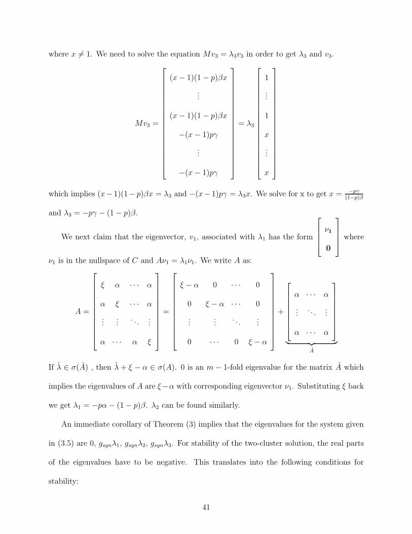
where x 6= 1. We need to solve the equation Mv3 = λ3v3 in order to get λ3 and v3.

Mv3 =

(x− 1)(1 − p)βx

...

(x− 1)(1 − p)βx

−(x− 1)pγ

...

−(x− 1)pγ

= λ3

1

...

1

x

...

x

which implies (x− 1)(1− p)βx = λ3 and −(x− 1)pγ = λ3x. We solve for x to get x = −pγ(1−p)β

and λ3 = −pγ − (1 − p)β.

We next claim that the eigenvector, v1, associated with λ1 has the form

ν1

0

where

ν1 is in the nullspace of C and Aν1 = λ1ν1. We write A as:

A =

ξ α · · · α

α ξ · · · α

......

. . ....

α · · · α ξ

=

ξ − α 0 · · · 0

0 ξ − α · · · 0

......

. . ....

0 · · · 0 ξ − α

+

α · · · α

.... . .

...

α · · · α

︸ ︷︷ ︸

A

If λ ∈ σ(A) , then λ + ξ − α ∈ σ(A). 0 is an m− 1-fold eigenvalue for the matrix A which

implies the eigenvalues of A are ξ−α with corresponding eigenvector ν1. Substituting ξ back

we get λ1 = −pα− (1 − p)β. λ2 can be found similarly.

An immediate corollary of Theorem (3) implies that the eigenvalues for the system given

in (3.5) are 0, gsynλ1, gsynλ2, gsynλ3. For stability of the two-cluster solution, the real parts

of the eigenvalues have to be negative. This translates into the following conditions for

stability:

41

• pα + (1 − p)β > 0

• pγ + (1 − p)α > 0

• pγ + (1 − p)β > 0

3.2.1 Application

In the previous chapter, we developed a phase model to explain the occurrence of traveling

waves in the olfactory lobe of Limax. The oscillators were coupled through all-to-all in-

hibitory synaptic coupling and local electrical coupling via gap junctions. Here, we want to

use the ideas and intuition from that paper and look at the contradicting effects of these two

couplings on the system. To accommodate what we want to achieve, we use the coupling

functions computed from the biophysical model in [13] with a slight modification. We only

change the coefficient of sin(2x) from −5 to 5. The coupling functions are:

Hsyn(x) = 35 + 200 cos(x) + 32 cos(2x) − 95 sin(x) + 5 sin(2x)

Hgap(x) = 87 − 50 cos(x) − 37 cos(2x) + 295 sin(x) − 65 sin(2x)

We remind the reader that the choice of coupling functions will determine what kind of

solutions we get. Changing the coefficient of sin(2x) in this manner allows for the existence

and stability of two-cluster states. Figure 3.2.1 represents the relation between p and φ. For

values of φ ranging from 0 to 2π, we are able to find the size of each cluster using (3.3).

From now on, we want to look at equal size clusters, so p = 1/2. In the case of different

size clusters, the Implicit Function Theorem can be used to get stability conditions for the

solutions. Substituting the value of p in (3.2) we get:

0 =gsyn2

[Hsyn(−φ) −Hsyn(φ)]

42

0 1 2 3 4 5 60

0.2

0.4

0.6

0.8

1

φ

p

Figure 3.2.1: Possible values for p are graphed as the phase difference, φ varies from 0 to 2π

43

Let g(x) = Hsyn(−x) −Hsyn(x). Hsyn is a 2π-periodic function so, 0 and π are fixed points

for g. For two oscillators, we need to have H ′syn(0) > 0 for the stability of the synchronous

state and H ′syn(π) > 0 for the stability of the two-cluster state which corresponds to the

anti-phase locked solution. The synchronous state was studied in ??.

Next, we compute the eigenvalues for the linearized system in order to determine the

stability of the two-cluster state with (p, φ) = (1/2, π). Figure 3.2.2 represents the values

of the eigenvalues for each possible value for the pair (p, φ). As we can see from the figure,

there is a small window of values of φ around π, where all the eigenvalues are negative. From

our stability conditions we need to satisfy:

• H ′syn(0) +H ′

syn(π) > 0,

• H ′syn(0) +H ′

syn(−π) > 0 and

• H ′syn(π) +H ′

syn(−π) > 0.

Since Hsyn is 2π-periodic, we have H ′syn(π) = H ′

syn(−π). We also know that H ′syn(0) < 0

and the last stability condition can be rewritten as H ′syn(π) > 0. Thus, the stability condition

in our case is:

• H ′syn(0) +H ′

syn(π) > 0

• H ′syn(π) > 0

• H ′syn(0) < 0

44

0 1 2 3 4 5 6−15

−10

−5

0

5

10

15

20

25

φ

λ1λ2λ3

Figure 3.2.2: Eigenvalues for the system in 3.5 are computed for all possible values of (p, φ).

45

3.3 THE FULL MODEL WITH GAP JUNCTIONS

Once we have a system with stable two-cluster state solutions, we want to see what hap-

pens to these solutions as we add small amounts of nearest neighbor gap junction coupling.

Equation (3.1) becomes

(3.6)dθjdt

=gsynN

N∑

k=1

Hsyn(θk − θj) + ggap[Hgap(θj+1 − θj) +Hgap(θj−1 − θj)]

where Hgap and ggap represent the gap junction coupling function and its strength, respec-

tively. Hsyn by itself promotes asynchrony, whereas Hgap has synchronizing effects. The

coupling functions are derived from the biophysical model given in [13], hence, Hsyn repre-

sents the synaptic inhibition between bursting neurons.

In Chapter 2, we looked at a network where the scope of the gap junctions extended

beyond the nearest neighbors. We found that in that case, a traveling wave was a stable

solution for all the values of the parameters. We want to see if this holds here also. We start

by noting that the traveling wave solution, θj = Ωt + 2πjN

, satisfies (3.6) where

Ω =gsynN

N∑

l=1

Hsyn(δl) + ggap(Hgap(δ) +Hgap(δ))

where δ = 2πN

. Given N , Hsyn, Hgap, gsyn and ggap, we can determine Ω uniquely up to sign.

We want to study the stability of the traveling wave solution. In order to avoid edge effects,

we assume the oscillators are arranged on a ring. The linearized system can be written as:

(3.7)dyjdt

=gsynN

N∑

l=1

H ′syn(δl)(yj+l − yj) + ggap[H

′gap(δ)(yj+1 − yj) +H ′

gap(−δ)(yj−1 − yj)]

The solutions for (3.7) are of the form yj = eλmteiδmj where j = 1, . . . , N , m = 0, . . . , N−

1. Solving for λm gives us:

46

λm =gsynN

N∑

l=1

H ′syn(δl)(e

iδml − 1) + ggap[H′gap(δ)(e

iδm − 1) +H ′gap(−δ)(e−iδm − 1)]

To determine the stability, we look at the real parts of λm. For m = 0, we have λ0 = 0

which corresponds to translation invariance. For m 6= 0, we need to use the Fourier series

expansions of H ′syn, and H ′

gap. Using the approximations for the coupling functions we see

that Re(λ2) becomes 0 when ggap = 0.0746gsyn for 20 oscillators. The imaginary part of λ2

is nonzero which means there is a Hopf bifurcation at this point. Considering different size

networks changes the value of ggap where the Hopf bifurcation occurs. Figure 3.3.1 displays

the values of critical coupling strength as N changes. For small networks, the traveling wave

is stable for a wide range of parameters, whereas as the network size grows, it loses stability

early on.

3.4 NUMERICAL RESULTS

In this section we numerically simulate a system of oscillators coupled with inhibition and

nearest neighbor gap junctions. The oscillators are arranged on a ring to avoid boundary

effects. Considering a linear array instead of the ring doesn’t change the qualitative behavior

of the system by a significant amount. Throughout this section, gsyn = 0.1. We vary ggap

between 0 and 0.1. In Section 3.2, we showed the existence and stability of two-cluster states

in the absence of gap junction coupling. Figure 3.4.1 displays the simulations done with 20

oscillators when ggap = 0. In Figure 3.4.1(a), random initial conditions lead to a solution

where half of the oscillators have the same phase and the rest are π apart. There are multiple

47

10 30 50 70 90 110 130 150 170 1900

0.1

0.2

0.3

0.4

0.5

0.6

0.7

0.8

number of oscillators

g gap

y=c*N2

Figure 3.3.1: Relation between ggap and N is shown by the blue ∗’s. The red line is the

curve that fits the data with y = cN 2 and c = 0.00002. gsyn is fixed at 0.1 throughout the

computation.

48

x[1..20]

time

40

0

0

6.28

time

40

0x[1..20]

(a) (b)

Figure 3.4.1: Two-cluster solution in a network with 20 oscillators where xj = θj − θ1.

(a) Random initial conditions converge to a two-cluster solution where the phase difference

between oscillators is either 0 or π. The number of oscillators in each cluster is the same.

(b) The two-cluster is solution is represented in this form for convenience.

49

ways to organize N oscillators in two equal-sized clusters. For computational convenience,

we consider the trivial case where the first N/2 oscillators are in one cluster and the rest

belongs to the other cluster. Such a solution is displayed in Figure 3.4.1(b). The two-cluster

solution is stable when there is no gap junction coupling present or when the coupling is

weak. Increasing ggap beyond 0.003491 results in a transcritical bifurcation as one of the

eigenvalues of the stability matrix crosses over to positive real axes.

When ggap = 0.1, there are several stable solutions to the system. One of them is the

traveling wave. This solution loses stability as ggap decreases. For N = 20, a Hopf bifurcation

occurs at ggap = 0.007463. To determine the stability of the periodic solutions, we can either

compute the coefficients for the normal form or we can use AUTO bifurcation package [12].

Figure 3.4.2 displays the whole bifurcation diagram. There is a region of bistability where we

have stable two-cluster state and stable periodic orbits. By perturbing the system enough,

we switch between these solutions.

We have seen that the value of ggap where the Hopf bifurcation occurs depends on the size

of the network. Figure 3.4.3 is a drawing that shows how the bifurcation diagram changes

as N changes. gc is the value of ggap where the two-cluster state becomes unstable and

gh is where the Hopf bifurcation is observed. We notice that regions of bistability change

drastically as N increases.

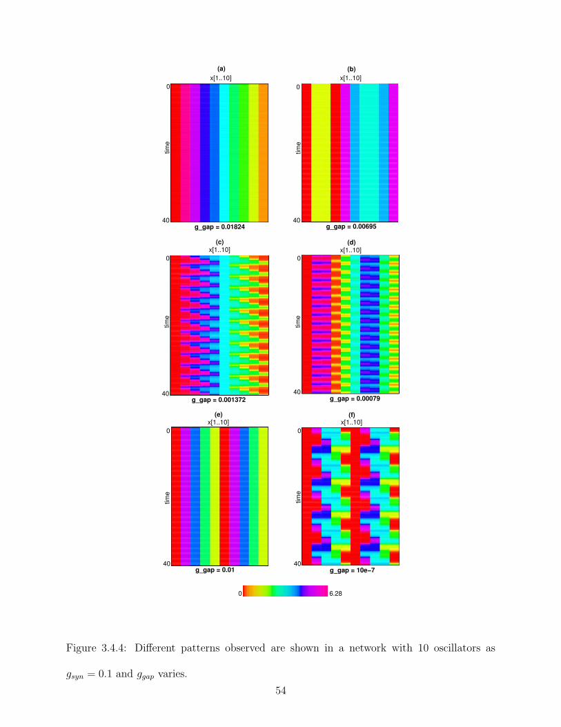
We now look at the simulations with 10 oscillators. Different from the other simulations

we see that there is also a patterned solution when ggap = 0.1. In Figure 3.4.4(a), we see a

regular traveling wave solution whereas panel (b) displays the plot for the patterned state.

Periodic orbits look like zig-zag patterns (panel (c)) and they eventually are replaced by

solutions that look like the ones in panel (d). There is another traveling wave solution for

50

x7

g_gap

HB

periodic orbits

2−cluster solution

STW

periodic orbits

region ofbistability

Figure 3.4.2: Bifurcation diagram as ggap varies for a system with 20 oscillators. Two-

cluster state becomes unstable at ggap = 0.003491. Branch of solutions bifurcating from

two-cluster state are drawn. Traveling waves become unstable through a Hopf bifurcation

at ggap = 0.007463. The periodic orbits are stable and they terminate at a homoclinic point.

There is a region where both the two-cluster state and periodic orbits are stable.

51

cggh gh

gh

ggap ggap

ggap

cg

cg

−1

4

−1

−1

4

4

X4 X8

X16

0 0.1

0.1

0.10

0

N = 10 N = 20

N = 40

Figure 3.4.3: Sketches of bifurcation diagrams for various N values. gc is the value of

ggap where the two-cluster state becomes unstable and gh is where the Hopf bifurcation is

observed. For N = 10, gc = 0.02759, gh = 0.001823; N = 20, gc = 0.003491, gh = 0.007463;

N = 40, gc = 0.003771, gh = 0.03045.

52

ggap = 0.01, where we see two waves in the ring (panel (e)). These become unstable at

another Hopf point where ggap is very close to 0. A new pattern of periodic solutions are

observed after this point (panel (f)).

Repeating the simulations with other N values, results in similar plots. We note that

it is possible to get waves going in both directions (clockwise and counter-clockwise). The

periodic zig-zag solutions doesn’t change in appearance, but the periodic solutions that we

get near the termination of the zig-zag patterns can be different. Figure 3.4.5 contains such

solutions where N = 20. With more oscillators, it is easier to see that the bifurcation from

the double traveling wave results in double zig-zag patterns. Figure 3.4.6 shows the transition

from traveling wave to periodic solutions.

3.5 CONCLUSIONS

We studied a system of globally coupled oscillators given in (3.1). Types of solutions possible

depends on the coupling function Hsyn. A widely studied example of such systems is the

Kuramoto model where the coupling is sinusoidal. To get the existence of n-cluster states

with n > 1, one needs to consider a coupling function with higher harmonics. We computed

Hsyn from a biophysical model and used an approximation by considering the dominant

Fourier modes. We have seen stable two-cluster states with equal cluster sizes π apart from

one another. It was also possible to see some different size clusters with p close to 1/2. We

focused our attention on the previous case.

Previous studies looked at globally coupled phase oscillators with addition of noise. Here

53

x[1..10]x[1..10]

x[1..10] x[1..10]

x[1..10] x[1..10]0 0

0

4040

40

0

40

00

4040

0 6.28

time

time

time

time

time

time

g_gap = 0.01824 g_gap = 0.00695

g_gap = 0.001372 g_gap = 0.00079

g_gap = 0.01 g_gap = 10e−7

(a) (b)

(c) (d)

(e) (f)

Figure 3.4.4: Different patterns observed are shown in a network with 10 oscillators as

gsyn = 0.1 and ggap varies.

54

x[1..20]0

40

x[1..20]0

40

time

time

(b)(a)

0 6.28

Figure 3.4.5: Before the periodic zig-zag solutions terminate, there is a new pattern observed.

For N = 20, (a) ggap = 0.00095 and (b) ggap = 0.0011.

55

x[1..20]0

40

time

0 6.28

Figure 3.4.6: A double traveling wave solution bifurcates into double zig-zag patterns for

N = 20 and ggap = 0.001.

56

we took a different path and added local gap junction coupling. Each oscillator was coupled

to its nearest neighbors via gap junctions. In pairwise connections, Hgap had a synchronizing

effect. The overall system behavior changed drastically as we added local gap junctions. Two-

cluster state lost its stability as we tuned ggap up and the system produced traveling waves.

We found that depending on the network size, the system displayed bistability between the

traveling wave and two-cluster solution and/or between the periodic zig-zag solution and

two-cluster solution. Changing the network size had drastic effects on network behavior in

this rather simple setting. In summary, we were able to analyze a system that has been long

studied with a twist and found very interesting behavior. We also want to point out that

our work has focused on the interplay of traveling waves and cluster solutions whereas other

studies on similar networks analyzed the synchronous solution and clusters of varying sizes

[3, 27, 31].

57

4.0 ASYNCHRONOUS SOLUTION

4.1 INTRODUCTION

Synchronization in populations of interacting elements has been the subject of study in

physical, biological, chemical settings. The goal is to find the underlying mechanism that

is responsible for collective behavior among the members of the given population. One way

of looking at the problem is to consider the elements as phase oscillators and study the

phase as time evolves. We demonstrated such examples in the previous chapters. In this

chapter, we examine a well-studied model for globally coupled phase oscillators. Kuramoto

analyzed a network of phase oscillators coupled through the sine of their phase differences

[43]. Without coupling each oscillator runs along the limit cycle attractor with an arbitrary

frequency. This model, which is simple yet non-trivial, has been the subject of many studies

to this date.

Since our aim is to analyze the effects of chemical and electrical coupling, we will study a

variation of the Kuramoto model with local gap junctions. We start this chapter by reviewing

the original model. In Section 4.2 we study the stability of asynchronous state in which the

phase of oscillators take on values in the interval [0, 2π] with equal probability. We calculate

the critical coupling strength where the asynchronous state becomes unstable for the original

58

and noise added systems.

In Section 4.3, we look at a collection of m groups of oscillators with each group consist-

ing of N members. Inside a group, the coupling structure is similar to what we have been

studying so far: each oscillator is connected to the rest of the oscillators in the group via a

combination of synaptic inhibition and gap junctions. Within groups, we assume each oscil-

lator in the collection is coupled to the rest of the oscillators in the collection via synaptic

inhibition and the oscillators in neighboring groups are coupled via gap junctions. Figure

4.1.1 displays an illustration of the network structure. We will study the stability of asyn-

chronous state as the coupling strength and noise in the system changes. We present our

numerical results in this section along with the analytical findings.

4.2 THE KURAMOTO MODEL

Collective synchronization can be seen in biological or physical examples such as flashing

fireflies, pacemaker cells in the heart and arrays of lasers. Winfree proposed that synchro-

nization can be studied in large networks of interacting limit-cycle oscillators where the

coupling between oscillators is weak [60]. His ideas were later used by Kuramoto to come

up with a general form for the dynamics of almost identical weakly coupled limit-cycle os-

cillators. Kuramoto’s model can be written down generally as follows:

θj = ωj +

N∑

k=1

Kjk(θk − θj), j=1, . . . , N(4.1)

where the dynamics of each oscillator is given by the phase of the oscillator , θj. ωj is the

natural frequency of oscillator j. The frequencies ωj are constant in time and distributed

59

12Group 1

Group 2Group 3

Group 4

Group 5

Group 6Group 7

Group 8

H

H21

H33

H33

g

g

oscillators

Figure 4.1.1: An illustrative figure of a collection of oscillators organized in m = 8 groups.

Each group consists of N = 12 oscillators. The red solid arrows represent the gap junction

coupling between groups, i.e, each oscillator in Group 1 is connected to each oscillator in

Group 2 and Group 3. The synaptic coupling is global in the sense that each oscillator in

the collection is coupled to the rest of the oscillators in the collection (black dashed lines

represent the synaptic coupling). Within each group the synaptic and gap junction coupling

is represented by a function Hjj for j = 1, 2, .., 8 (red dashed lines represent this combination

coupling).

60

according to some probability density g(ω). Without loss of generality we assume that

g(ω) is symmetric about the mean value 0. The form of coupling taken by Kuramoto is

Kjk = KN

sin(θk − θj). Using mean-field theory, we can analyze the system. The complex

order parameter r is defined as

reiψ =1

N

N∑

k=1

eiθk(4.2)

Multiplying both sides by e−iθj and taking the imaginary parts results in

r sin(ψ − θj) =1

N

N∑

k=1

sin(θk − θj)

Thus, the Kuramoto model can be written as

θj = ωj +Kr sin(ψ − θj)(4.3)

where Kr is the mean-field strength and ψ is the mean phase. If r is independent of time,

solving (4.3) and substituting the solutions in (4.2) gives us a self-consistent equation for r.

This tells us that there is a phase transition at some critical value of the coupling strength.

The order parameter is zero for K < Kc and becomes nonzero afterwards. Macroscopic

oscillations are seen after the transition point. They are later entrained to one collective

oscillation. In other terms, there is a critical value of the coupling strength below which the

asynchronous state is stable and later as we increase K, the oscillators are synchronized and

r approaches 1. Kuramoto’s original analysis uses the self consistency condition for r and an

assumption about the distribution to solve for Kc. The reader is referred to review papers

for details of Kuramoto’s original derivation and other approaches [1, 53].

We will give the derivation using Strogatz’s approach of using a probability density

function ρ(θ, ω, t) in the limit of infinitely many oscillators. For each natural frequency ω,

61

we imagine a continuum of oscillators distributed on the circle. Let ρ(θ, ω, t)dθ to denote is

the fraction of oscillators with phase that lies in the interval [θ, θ+dθ]. The equation for the

order parameter given in (4.2) can be written as an average over phase and frequency

(4.4) reiψ =

∫ 2π

0

∫ ∞

−∞

eiθρ(θ, ω, t)g(ω)dωdθ.

ρ is non-negative, 2π-periodic in θ and satisfies the normalization condition

(4.5)

∫ 2π

0

ρ(θ, ω, t)dθ = 1

for all values of the natural frequency ω and t. Note that the oscillators move with velocity

(4.6) v(θ, ω, t) = ω +Kr sin(ψ − θ).

We derive a continuity equation for the oscillator density by

(4.7)∂ρ

∂t+

∂

∂θ(ρv) = 0

Using (4.4) and (4.6), (4.7) can be written as:

(4.8)∂ρ

∂t=

∂

∂θ

[

ρ

(

ω +K

∫ 2π

0

∫ ∞

−∞

sin(θ′ − θ)ρ(θ′, ω′, t)g(ω′)dω′dθ′)]

This equation is the continuum limit for the Kuramoto model. We will study the existence

and stability of asynchronous solution for the Kuramoto model using (4.8). Asynchronous

solution is the case where each phase in [0, 2π] is taken by the oscillators with same prob-

ability. In this case r = 0 and ρ = 1/2π. Substituting ρ in (4.8) we see that this is

indeed a solution to the Kuramoto model. Next, we study the stability of this solution. Let

62

ρ(θ, ω, t) = 12π

+ ν(θ, ω, t) in (4.7) where ν is a small perturbation from the asynchronous

solution. We study the linear stability problem by neglecting the nonlinear terms in ν

∂ν

∂t= − ∂

∂θ

[

ων +K

2π

∫ ∞

−∞

g(ω)dω

∫ 2π

0

ν(φ, ω, t) sin(φ− θ)dφ

]

(4.9)

Solutions to (4.9) are of the form ν(θ, ω, t) = eλtΨ(ω)eiθ.

Substituting this into (4.9) gives us

λΨ(ω)eiθeλt = −iωΨ(ω)eiθeλt

+K

2π

∫ ∞

−∞

g(ω)dω

∫ 2π

0

eiθeλtΨ(ω) cos(φ− θ)dφ(4.10)

Canceling eλt from both sides of the equation and letting φ′ = φ − θ, we rewrite (4.10)

as

λΨ(ω)eiθeλt = −iωΨ(ω)eiθeλt +K

2πeiθeλt

∫ ∞

−∞

Ψ(ω)g(ω)dω

∫ 2π−θ

−θ

eiφ′

cos(φ′)dφ′

We can now cancel out eiθ. Note that∫ 2π−θ

−θf(φ)dφ =

∫ 2π

0f(φ)dφ for a 2π-periodic function

f . The final form of the equation is:

λΨ(ω) = −iωΨ(ω) +K

2π

∫ ∞

−∞

Ψ(ω)g(ω)dω

∫ 2π

0

eiφ′

cos(φ′)dφ′(4.11)

Noticing that∫ 2π

0eiφ

′

cos(φ′)dφ′ = π and letting A =∫∞

−∞Ψ(ω)g(ω)dω, we rewrite (4.11)

as:

λΨ(ω) = −iωΨ(ω) +K

2A

63

Solving for Ψ(ω) gives us the equation

Ψ(ω) =K

2

A

(λ+ iω)

Substituting Ψ(ω) in the equation for A, we now can write

A =

∫ ∞

−∞

g(ω)KA

2(λ+ iω)dω

⇔ 1 =K

2

∫ ∞

−∞

g(ω)

λ+ iωdω

If we take g(ω) to be even and unimodal, we see that there is at most one solution for λ

which is real when exists. We write the last equation as

1 =K

2

∫ ∞

−∞

g(ω)(λ− iω)

λ2 + ω2dω

⇔ 1 =K

2

∫ ∞

−∞

λg(ω)

λ2 + ω2dω − i

K

2

∫ ∞

−∞

ωg(ω)

λ2 + ω2dω

and note that the second integral in the last equation is zero. The final form of the

equation is

(4.12) 1 =K

2

∫ ∞

−∞

λg(ω)

λ2 + ω2dω

Equation (4.12) implies that the eigenvalue λ ≥ 0 so the asynchronous state is not linearly

stable. For values of λ→ 0+ the integral∫∞

−∞

λg(ω)λ2+ω2dω → πg(0) , so we recover the value of

the critical coupling strength, Kc, found by Kuramoto in the form

(4.13) 1 =1

2Kcπg(0)

64

Strogatz proves the neutral stability of the asynchronous solution using this method in

his paper with Mirollo [54]. Sakaguchi also studied the Kuramoto model and its extension

by allowing fluctuations in natural frequencies [51].

Here is the equation governing the phase changes:

θi = ωi + ξi(t) +K

N

N∑

j=1

sin(θj − θi)(4.14)

where ξi’s are white noise processes with zero mean and σ2 as power spectral density. We

use similar analysis as before to write down the continuity equation

(4.15)∂ρ

∂t=σ2

2

∂2ρ

∂θ2− ∂

∂θ(ρν)

After these modifications, the results given earlier change slightly

λ ¯Ψ(ω) = −iωΨ(ω) +K

2A− σ2

2Ψ(ω)

Let D = σ2/2, and solve for Ψ(ω)

Ψ(ω) =K

2

A

λ+ iω +D

Substitute this into the equation for A to get

A =K

2

∫ ∞

−∞

A

λ+ iω +Dg(ω)dω

⇔ 1 =K

2

∫ ∞

−∞

g(ω)

(λ+D + iω)dω(4.16)

Solutions to (4.16) are the eigenvalues for the linear stability problem for the Kuramoto

model with noise. When random noises are added, the mutual entrainment (synchronization)

becomes less clear. Thus, the random noises make the critical coupling strength Kc larger

without any quantitative change with respect to phase transition. For further details on the

calculations, the reader is referred to [54, 9, 51].

65

4.3 KURAMOTO MODEL WITH GAP JUNCTIONS

In this section, we extend the Kuramoto model to allow for local coupling between oscillators.

We consider a network of mN oscillators organized in m groups with each group consisting of

N oscillators. The oscillators are globally coupled via synaptic inhibition. The gap junction

coupling is local in the sense that each oscillator is connected to other oscillators in the

nearest neighbor groups and the group to which it belongs. So each oscillator makes 3N

electrical synapses (see Figure 4.1.1). For m = 2, 3, the coupling is all:all. For m > 3, we

write down a set of equations for the network:

(4.17)dθijdt

= ξij(t) +1

N

N∑

l=1

(m∑

k=1

Hjk(θlk − θij)

)

i=1, . . . , N j=1, . . . , m

where ξij’s are white noise processes with zero mean and σ2 is the power spectral density,

Hjk’s are the coupling functions (their form will be given explicitly later in the section). Note

that (4.17) differs from the Kuramoto model in the sense that we do not have the arbitrary

natural frequencies. Instead, heterogeneity is introduced via the noise process.

As in Section 4.2, we want to study the existence and stability of the asynchronous solu-

tion. We will use the probability density approach. Let ρ(θ1, θ2, . . . , θm, t) be the probability

distribution for oscillators in m groups having phases θ1, . . . , θm at time t. ρ satisfies the

normalization condition

∫ 2π

0

. . .

∫ 2π

0

ρ(θ1, θ2, . . . , θm, t)dθ1 . . . dθm = 1

66

which is a generalized form of (4.5). ρ is 2π-periodic in its first m arguments. From Sak-

aguchi’s formulation [51], we can write down a Fokker-Planck equation for ρ

∂ρ

∂t=

σ2

2(∂2ρ

∂θ21

+ · · ·+ ∂2ρ

∂θ2m

)

−m∑

j=1

∂

∂θj

ρ(Θ, t)

∫ 2π

0

. . .

∫ 2π

0

ρ(Φ, t)

m∑

k=1

Hjk(θk − θj)dφ1 . . . dφm

(4.18)

where Θ = (θ1, . . . , θm) and Φ = (φ1, . . . , φm). We define the marginal distribution for θi:

ρi(θ) =

∫ 2π

0

. . .

∫ 2π

0

ρ(φ1, . . . , φi−1, θ, φi+1, . . . , φm)∏

φj:j 6=i

dφj

Let us illustrate the case where m = 2. We rewrite (4.18) as:

∂ρ

∂t=

σ2

2(∂2ρ

∂θ21

+∂2ρ

∂θ22

)

− ∂

∂θ1

ρ(θ1, θ2)

∫ 2π

0

∫ 2π

0

ρ(φ1, φ2) [H11(φ1 − θ1) +H12(φ2 − θ1)] dφ1dφ2

− ∂

∂θ2

ρ(θ1, θ2)

∫ 2π

0

∫ 2π

0

ρ(φ1, φ2) [H21(φ1 − θ2) +H22(φ2 − θ2)] dφ1dφ2

(4.19)

Integrating both sides of the equation (4.19) with respect to θ1 and θ2 and using the defini-

tions for marginals, we can write (4.19) as a system of two partial differential equations:

∂ρ1(θ1)

∂t=

σ2

2

∂2ρ1(θ1)

∂θ21

− ∂

∂θ1

[

ρ1(θ1)

∫ 2π

0

ρ1(φ1)H11(φ1 − θ1)dφ1

]

− ∂

∂θ1

[

ρ1(θ1)

∫ 2π

0

ρ2(φ2)H12(φ2 − θ1)dφ2

]

∂ρ2(θ2)

∂t=

σ2

2

∂2ρ2(θ2)

∂θ22

− ∂

∂θ2

[

ρ2(θ2)

∫ 2π

0

ρ1(φ2)H21(φ1 − θ2)dφ1

]

− ∂

∂θ2

[

ρ2(θ2)

∫ 2π

0

ρ2(φ2)H22(φ2 − θ2)dφ2

]

Let’s define H11 = H22 ≡ H and H12 = H21 ≡ G so that H is the function representing

interactions within a group and G represents interactions between groups. Two solutions to

the system given can be characterized as follows:

67

• ρ1(θ) = ρ2(θ) ⇒ Group 1 and Group 2 are in-phase synchronized

• ρ1(θ) = ρ2(θ − π) ⇒ Group 1 and Group 2 are anti-phase synchronized

In order to study the existence and stability of the asynchronous state, we write down

the system given above in the following form

(4.20)

∂ρj(θ, t)

∂t=σ2

2

∂2ρj∂θ2

− ∂

∂θ

ρj(θ)

[∫ 2π

0

ρj(φ)Hjj(φ− θ)dφ+

∫ 2π

0

ρk(φ)Hjk(φ− θ)dφ

]

for j = 1, 2. Note that the derivation of these equations for m > 2 is similar. It is easy

to see that ρj(θ) = 1/2π is a solution to (4.20). We take a perturbation of the asynchronous

solution, ρj(θ, t) = 12π

+ νj(θ, t), and write the equation for the linear stability problem

excluding nonlinear terms

∂νj∂t

=σ2

2

∂2νj∂θ2

− ∂

∂θ

[νj(θ2)Hjj + Hjk

]

− ∂

∂θ

[1

2π

∫ 2π

0

Hjj(φ− θ)νj(φ) +Hjk(φ− θ)νk(φ)

]

(4.21)

where Hjj and Hjk are the average values of the coupling functions over a period. The

solutions to (4.21) are of the form νj = eλteinθvj where vj is a constant. Substituting νj

into (4.21) and using the information about the periodicity of the functions Hjk, we get an

equation for the eigenvalue λ

λvj = −σ2n2

2vj − inΩjvj +

1

2π

∫ 2π

0

m∑

k=1

H ′jk(φ)vke

inφdφ

where Ωj =∑

k Hjk. If the coupling functions satisfy Hjk = Hj−k (mod m), the eigen-

value problem can be rewritten as

(4.22) λnvj = −(inΩj +σ2n2

2)vj +

m−1∑

k=0

αj−k(n)vk

68

where

αj−k(n) =1

2π

∫ 2π

0

H ′jk(φ)einφdφ

is the nth complex Fourier term for the function H ′jk. If we were to write this equation as a

linear system λv = Av, the matrix A has a special structure. It is a circulant matrix and

the eigenvectors have the following form:

vT = [1 e2πij/m . . . e2πi(m−1)j/m]T

Thus, we derive the equation for the eigenvalues as

λn = −inΩ − n2σ2

2+ α(l, n)

with α(l, n) =∑m−1

k=0 αk(n)e2πkl/m. If we look at the real parts of the eigenvalues, we see

that the stability of the asynchronous solution depends on the interplay between the noise

strength and the harmonic terms for the coupling function.

We now present some simulation results with 600 oscillators. The oscillators are divided

into 6 groups with equal size and the coupling structure is described above. We chose a

simple form for the coupling functions: global coupling function is chosen as − sin(x) and

local coupling is k sin(x) where k is a positive coupling strength. Figure 4.3.1 displays the

results of the simulations where actual phases of the oscillators are plotted in time. In

panel (a), we see that asynchrony is a solution in the absence of gap junction coupling. By

adding small amounts of gap junctions (k 6= 0), we see the emergence of a traveling wave-like

solution where the oscillators in in the same group tend to synchronize to the same phase

while preserving a phase difference among different groups (panel (b)). Increasing the gap

junction coupling strength makes this pattern more visible (panel (c)). In panel (d), we

present the case with no noise added where we get a regular traveling wave solution.

69

6.280

Oscillator # Oscillator #

Oscillator # Oscillator #

6001

600600

6001

1

10 10

1010

10

00

0

(b)(a)

(c) (d)

time

time

time

time

Figure 4.3.1: A network of 600 oscillators organized in 6 equisized groups. (a) Asynchronous

solution with D = σ2/2 = 0.05 and k = 0, (b) Gap junction coupling disrupts the asyn-

chronous solution, k = 0.01, (c) for k = 0.04 the traveling wave like solution becomes more

visible, (d) traveling wave solution with no noise and k = 0.04.

70

4.4 CONCLUSIONS

In this chapter, we have studied one of the most widely studied models for globally coupled

oscillators. Since the time the Kuramoto model was introduced in 1975, there have been

many papers published about the model and its extensions. Despite the simple form of the

model, it displays rich behavior and there are still open problems related to the model.

We first reviewed the Kuramoto model and its version with added noise. We looked

at the linear stability problem for the asynchronous solution. The original model lacks

spatial structure. By adding local gap junctions, we saw that the asynchronous state loses

stability and traveling wave solutions emerge. In the original model, the asynchronous state

becomes unstable as the coupling strength increases and the oscillators become synchronous

or partially synchronous. We don’t see synchrony in our case but the gap junction coupling

helps synchronize the oscillators belonging to the same group and create a phase difference

with the other groups.

This chapter is still work in progress and we will continue to study this case in depth.

71

5.0 DISCUSSION

In this thesis, we examine a network of phase oscillators coupled through electrical and

chemical synapses. We study how each type of coupling effects the stability of synchrony,

clustered state and asynchrony.

In the first chapter, we study the synchronous solution. Our work is inspired by earlier

studies done with Limax where traveling waves were observed without a frequency gradient.

We use a phase model to represent the interactions between oscillators. The electrical and

chemical synapses have counter acting effects on synchrony. Global inhibition supports anti-

phase synchrony and local gap junctions promote in-phase synchrony when a pair of identical

oscillators are considered. In the absence of synaptic inhibition, the system is synchronized

with no phase lag, but as the strength of the synapses increase there is a bifurcation to a

state where there is a localized stable pattern of activity is observed. We derive the normal

form equation for the bifurcation. Further increasing the coupling strength results in another

bifurcation where the intermediate state transitions to the traveling wave. This traveling

wave solution exists and is stable for all values of the parameters. Our numerical results

support the analytical results found in this chapter and we are able to explain the existence

of traveling waves in a seemingly homogeneous, symmetric system.

In the second chapter, we study the clustered solutions where the oscillators are divided

72

into subgroups with similar activity patterns. The model we consider is similar in structure

to the model in the first chapter with very few modifications. We specifically look at the

two-cluster state where half of the oscillators have the same phase and they differ by the

same amount from the rest of the oscillators. This solution is stable when there is no gap

junction coupling, and loses stability with the addition of even a small amount. Since we

know the existence of traveling wave solutions from the previous chapter, we look for them

here. We see that the traveling wave solution becomes unstable via a Hopf bifurcation. We

compute the bifurcation diagrams for various network sizes. The system exhibits bistability

depending on the network size.

In the last chapter, we look at a modified version of the Kuramoto model where we allow

for local coupling. We go over the Kuramoto model and study the existence and stability

of asynchronous solution. We see that the asynchronous solution loses stability and again

the network goes to a traveling wave solution. This is different than the outcome with

the original Kuramoto model where synchronous solution emerges as the coupling strength

increases.

In this work, we have seen that inhibition and gap junction coupling do not necessarily

have a complementary effects on network behavior of coupled oscillators. We have observed

that addition of local gap junctions enrich the dynamics of a symmetric globally coupled

network with synaptic coupling. Gap junctions support the emergence of traveling waves.

We have looked at the problem from three different perspectives and traveling wave behavior

was dominant in each of them. We have shown that pattern formation can be observed even

in a network with a simple architecture.

73

APPENDIX A

A.1 PHASE MODEL AND AVERAGING

We study the effects of electrical and chemical coupling in a network of phase oscillators.

The phase model we study in Chapter 2 is derived from a biophysical model. Since we will

use this reduction throughout the thesis, we state the theorems that enable us to proceed

this way. The first theorem was proven by Art Winfree and John Guckenheimer in 1970s

and it has been implemented by many researchers since then [25, 28, 34, 43, 47].

Theorem 4 Phase Model

Let the following equation

(A.1) X = F (X), X ∈ Rm

represent a dynamical system which has an exponentially stable limit cycle γ ∈ Rm with

period 2π so that every trajectory γ with an initial point ˆγ(0) in a small neighborhood of γ

stays in that neighborhood as t→ ∞. Then, the dynamical system given by

(A.2) θ = 1, θ ∈ S1

is a canonical model for all systems that are represented by ( A.1).

74

Proof of this theorem can be found in [34]. A model is canonical if there is a continuous

change of variables that transforms any other model from the family into this one [34]. The

use of canonical models has many advantages. First, these models are simpler than the

original dynamical system. We can derive the canonical model even when F is not given

explicitly. The only requirement is that the system has a limit cycle attractor. We have

to keep in mind that these models only tell us the local behavior. In order to get global

information, one needs to use other tools.

Since we are studying coupled oscillators we need a modified version of Theorem 4. There

are several types of coupling: pulsatile, strong and weak. In the case of weak coupling, the

system can be written as:

(A.3) Xi = Fi(Xi, λ) + εGi(X, λ, ρ, ε), i=1, . . . , n

where ε is small enough. Assume that there is a value of the parameter λ such that the

uncoupled system

(A.4) Xi = Fi(Xi, λ), Xi ∈ Rn

has a stable limit cycle attractor γi ∈ Rn. As we showed in Theorem (4), we can describe

the activity on the limit cycle in terms of the phase θ ∈ S1 of oscillation

θi = Ωi(λ)

where Ωi is the natural frequency of the oscillations. Similarly, we can define the behavior

of the coupled system with:

θi = Ωi(λ) + εgi(θ, λ, ρ, ε), i=1, . . . , n

75

The latter has been proven using different approaches over the years. Winfree used phase

response curves and Malkin’s theorem uses the Fredholm Alternative to solve the adjoint

problem. We will only discuss Malkin’s method here.

Theorem 5 Malkin’s Theorem for Weakly Coupled Oscillators

Consider the weakly coupled system

Xi = Fi(Xi) + εGi(X), texti = 1, . . . , n

where the uncoupled system (ε = 0) has stable 2π-periodic limit cycle solutions γi ∈ Rn. Let

τ = εt be slow time and let φi(τ) ∈ S1 be the phase deviation from the natural oscillation

γi(t), t ≥ 0. The vector of phase deviations φ = (φ1, . . . , φn)T ∈ T n is a solution to

φ′i = Hi(φ− φi, ε), i=1, . . . , n

where ′ = d/dτ , the vector φ− φi = (φ1 − φi, . . . , φn − φi)T and the function

Hi(φ− φi, 0) =1

2π

∫ 2π

0

Qi(t)TGi(γ(t+ φ− φi))dt

where Qi(t) ∈ Rn is the unique non-trivial 2π- periodic solution to the system

Q′i = −DFi(γi(t))Qi

satisfying the normalization condition Qi(0)TFi(γi(0)) = 1.

Weak coupling allows us to use the method of averaging to reduce the model to a system

of phase equations. In this approach, each oscillator is represented by a single variable, phase,

that lies on S1. Interactions between two connected oscillators depends on the difference of

phases.

76

A.2 BIOPHYSICAL MODEL AND COUPLING FUNCTIONS

We use the biophysical model given in [13]. Each uncoupled bursting cell in the Limax model

has the form:

CdV

dt= −IL − IK − ICa

= −gL(V − EL) − gKn4(V − EK) − gCam

2h(V − ECa)

where n, h obey the equations:

dn

dt= .075[an(V )(1 − n) − bn(V )n]

dh

dt= 1.125(h∞(V ) − h)/τh(V )

with

an(V ) = .032(−48 − V )/(exp(−(48 + V )/5) − 1)

bn(V ) = .5 exp(−(43 + V )/40)

h∞(V ) = 1/(1 + exp((V + 86)/4))

τh(V ) = if (V < (−80))

then (exp((V + 470)/66.6))

else (28 + exp((V + 25)/− 10.5))

The activation gate for the T-type calcium current has the form:

m(V ) = 1/(1 + exp(−(V + 60)))

The parameters are C = 2.66, gK = 5, gL = 0.024, gCa = 2, EK = −90, ECa = 140,

EL = −82, and Esyn = −78.

77

Using this model in XPPAUT [22], we compute one full cycle of the periodic orbit. Once

we have a nice periodic orbit, we use the Averaging tool under Numerics menu to compute

the adjoint. The adjoint is then used by XPPAUT to get the interaction functions. We

take the dominating terms which are usually the first 2 or 3 terms that appear in the Data

Viewer. For detailed examples, the reader is referred to the manual for XPPAUT [22].

In our case, the approximations of coupling functions are as follows:

Hsyn(x) = 35 + 200 cos(x) + 32 cos(2x) − 95 sin(x) − 5 sin(2x)

Hgap(x) = 87 − 50 cos(x) − 37 cos(2x) + 295 sin(x) − 65 sin(2x)

78

APPENDIX B

To calculate the normal form for the bifurcation, we match the “ε” terms from (2.12):

Ω1 =

∫ 2π

0

A1(y′) [ψ1(x− y′) − ψ1(x)] dy

′ ≡ L ψ1

We integrate both sides of the equation with respect to x to get Ω1 = 0. If we solve

Lψ1 = 0, we get that ψ1(x) = zeix + ze−ix without loss of generality. Next, we look at

ε2terms

Ω2 = L ψ2 +

∫ 2π

0

A2(y′) [ψ1(x− y′) − ψ1(x)]

2 dy′

+g1α1

2π

∫ 2π

0

[ψ1(x− y′) − ψ1(x)] dy′(B.1)

Substitute ψ1 in the above equation and multiply both sides of the equation by 1 and

integrate w.r.to x

∫ 2π

0

Ω2 dx = 8π z z [B0(A2) − B1(A2)]

Ω2 = 4z z [B0(A2) −B1(A2)]

79

where Bn(Aj) =∫ 2π

0Aj(y

′) e±iny′

dy′ , j = 1, 2, 3. Now, we multiply ( B.1) by e−ix

0 = −2π g1 α1 z

which implies g1 = 0. So, we can write gsyn = g∗syn + ε2g2 and we solve for ψ2

0 = L ψ2 + (z2e2ix + z2e−2ix) [B2(A2) +B0(A2) − 2B1(A2)](B.2)

We now propose that ψ2 = C z2e2ix + C z2e−2ix and substitute back in ( B.1)

0 = [B2(A1) − B0(A1)] (C z2e2ix + C z2e−2ix)

+[B(A2) +B0(A2) − 2B1(A2)] (z2e2ix + z2e−2ix)

Looking at the coefficients of z2 term gives

C =2B1(A2) − B2(A2) − B0(A2)

B2(A1) −B0(A1)(B.3)

We have to make sure here that the denominator is non-zero. This is easy to see since

B2(A1) − B0(A1) = 0 would imply that g∗syn = gSβ1(I2−1)α2

which is not true since g∗syn =

ggapβ1(I1−1)α2

and I1 > I2.

Next, we look at “ε3” terms

80

Ω3 = L ψ3 +

∫ 2π

0

A3(y′) [ψ1(x− y′) − ψ1(x)]

3 dy′

+2

∫ 2π

0

A2(y′) [ψ1(x− y′)ψ2(x− y′) + ψ1(x)ψ2(x)] dy

′

−2

∫ 2π

0

A2(y′) [ψ1(x− y′)ψ2(x) + ψ1(x)ψ2(x− y′)] dy′

+g2α1

2π

∫ 2π

0

[ψ1(x− y′) − ψ1(x)] dy′(B.4)

Let’s look at the terms in ( B.4) closely

[ψ1(x− y′) − ψ1(x)]3 = [zeixe−iy

′

+ ze−ixeiy′ − zeix − ze−ix]3

= z3e3ixe−3iy′ + 3z2zeixe−iy′

+ 3zz2e−ixeiy′

+ z3e−3ixe3iy′

−3z3e3ixe−2iy′ − 3z2zeixe−2iy′ − 6z2zeix

−6zz2e−ix − 3zz2e−ixe2iy′ − 3z3e−3ixe2iy

′

+3z3e3ixeiy′

+ 3z2zeixeiy′

+ 6z2zeixe−iy′

+6zz2e−ixeiy′

+ 3zz2e−ixe−iy′

+ 3z3e−3ixeiy′

−z3e3ix − 3z2zeix − 3zz2e−ix − z3e−3ix

Let T = [ψ1(x− y′)ψ2(x− y′) + ψ1(x)ψ2(x) − ψ1(x− y′)ψ2(x) − ψ1(x)ψ2(x− y′)], then

81

T = [(zeixe−iy′

+ ze−ixeiy′

)(Cz2e2ixe−2iy′ + Cz2e−2ixe2iy′

)

+(zeix + ze−ix)(Cz2e2ix + Cz2e−2ix)

−(zeixe−iy′

+ ze−ixeiy′

)(Cz2e2ix + Cz2e−2ix)

−(zeix + ze−ix)(Cz2e2ixe−2iy′ + Cz2e−2ixe2iy′

)

= Cz3e3ixe−3iy′ + Czz2e−ixeiy′

+ Cz2zeixe−iy′

+Cz3e−3ixe3iy′

+ Cz3e3ix + Czz2e−ix

+Cz2zeix + Cz3e−3ix − Cz3e3ixe−iy′ − Czz2e−ixe−iy

′

−Cz2zeixeiy′ − Cz3e−3ixeiy

′

−Cz3e3ixe−2iy′ − Czz2e−ixe2iy′

−Cz2zeixe−2iy′ − Cz3e−3ixe2iy′

Substituting ψ1 and ψ2 in ( B.4) and using the expansions for [ψ1(x− y′) − ψ1(x)]3 and

T , we then multiply both sides of B.4 by 1 and integrate w.r.to x to get Ω3 = 0. Next,

multiply both sides by e−ix and integrate with respect to x

0 = z2z

∫ 2π

0

A3(y′) [9e−iy

′

+ 3eiy′ − 3e−2iy′ − 9] dy′

+2C z2z

∫ 2π

0

A2(y′) [e−iy

′ − eiy′ − e−2iy′ + 1] dy′ − g2α1z

we can simplify this as follows

0 = z2 z[12B1(A3) − 3B2(A3) − 9B0(A3) + 2C B0(A2) − 2CB2(A2)] − g2α1z

82

by letting ζ = 12B1(A3)− 3B2(A3)− 9B0(A3) + 2C B0(A2)− 2CB2(A2) and η = −g2α1

we have the normal form at the bifurcation point as

0 = ζz2z + ηz

83

BIBLIOGRAPHY

[1] J. A. Acebron, L. L. Bonilla, C. J. Perez, F. Ritort and R. Spigler, The Kuramoto

Model: a simple paradigm for synchronization phenomena, Reviews of Modern

Physics 77(1) (2005) pp.137-185

[2] P. Ashwin and J. W. Swift, The Dynamics of n Weakly Coupled Oscillators, J.

Nonlinear Sci. 2 (1992) pp.69-108

[3] M. Banaji, Clustering in Globally Coupled Oscillators, Dynamical Systems 17(3)

(2002) pp.263-285

[4] T. Bem and J. Rinzel, Short Duty Cycle Destabilizes a Half-center Oscillator,but

Gap Junctions Restabilize the Anti-phase Pattern, J. Neurophysiol. 91 (2004)

pp.693-703

[5] T. Bem, Y. LeFeuvre, J. Simmers and P. Meyrand, Electrical Coupling Can Prevent

Expression of Adult-like Properties in an Embryonic Neural Circuit, J. Neurophys-

iol. 87 (2002) pp.538-547

[6] C. Bou-Flores and A. J. Berger, Gap junctions and Inhibitory Synapses Modulate

Inspiratory Motoneuron Synchronization, Neurophysiol. 85 (2001) pp.1543-1551

[7] E. Brown, P. Holmes and J. Moehlis, Globally Coupled Oscillator Networks, In:

Perspectives and problems in Nonlinear Science: A celebratory Volume in Honor

of Larry Sirovich, editors:E. Kaplan and J. Marsden and K. Sreenivasan, Springer,

New York, (2003) pp.183-215

[8] C. C. Chow and N. Kopell, Dynamics of Spiking Neurons With Electrical Coupling,

Neural Comp. 1 (1994) pp.313-321

84

[9] J. D. Crawford, Amplitude Expansions for Instabilities in Populations of Globally

Coupled Oscillators, J. Stat. Phys. 74 (1994) pp.1047-1084

[10] J. D. Crawford, Scaling and Singularities in the Entrainment of Globally Coupled

Oscillators, Phys. Rev. Lett. 74(21) (1995) pp.4341-4344

[11] J. D. Crawford and K. T. R. Davies, The Behavior of Rings of Coupled Oscillators

, Physica D 125 (1999) pp.1-46

[12] E. Doedal, AUTO: A program for the automatic bifurcation analysis of autonomous

systems, Congr. Numer. 30 (1981) pp. 265-284

[13] B. Ermentrout, J. W Wang, J. Flores and A. Gelperin, Model for Transition from

Waves to Synchrony in the Olfactory Lobe of Limax, J. Comput. Neurosci. 17 (2004)

pp.365-383

[14] G. B. Ermentrout and D. Kleinfeld, Travelling Electrical Waves in Cortex:Inside

from Phase Dynamics and Speculation on a Computational Role, Neuron 29 (2001)

pp.33-44

[15] B. Ermentrout, J. Flores and A. Gelperin, Minimal Model of Oscillations and Waves

in the Limax Olfactory Lobe with Tests of the Model’s Predictive Power, J. Neuro-

physiol. 79 (1998) pp.2677-2689

[16] B. Ermentrout, J. W Wang, J. Flores and A. Gelperin, Model for Olfactory Dis-

crimination and Learning in Limax procerebrum Incorporating Oscillatory Dynam-

ics and Wave Propagation, J. Neurophysiol. 85 (2001) pp.1444-1452

[17] G. B. Ermentrout and N. Kopell, Inhibition-Produced patterning in Chains of Cou-

pled Nonlinear Oscillators, Siam J. Appl. Math. 54(2) (1994) pp.478-507

[18] G. B. Ermentrout, Neural Networks as Spatio-Temporal Pattern-Forming Systems,

Rep. Prog. Phys. 12 (2000) pp.1643-1678

[19] G. B. Ermentrout, Stable periodic solutions to Discrete and Continuum Arrays of

Weakly Coupled Nonlinear Oscillators, Siam J. Appl. Math. 52(6) (1992) pp.1665-

1687

85

[20] G. B. Ermentrout, The Behavior of Rings of Coupled Oscillators, J. Math. Biology

23 (1985) pp.55-74

[21] Ermentrout, G.B n:m Phase-Locking of Weakly Coupled Oscillators J. Math. Biol-

ogy 12, 327-342 (1981)

[22] B. Ermentrout, Simulating, Analyzing, and Animating Dynamical Systems: A

Guide to XPPAUT for Researchers and Students, Software Environ Tools 14, SIAM,

Philadelphia, 2002

[23] G.B. Ermentrout, Stable small amplitude solutions in reaction diffusion systems,

Quart Appl Math, 39 (1981), pp.61-86

[24] B. Ermentrout, Type I membranes, phase resetting curves, and synchrony, Neural

Comput. 8 (1996), pp. 979-1001

[25] G. B. Ermentrout and N. Kopell, Multiple Pulse Interactions and Averaging in

Systems of Coupled Neural Oscillators,J. Math. Biol. 29(3) (1991) pp.195-217

[26] M. Galarreta and S. Hestrin A network of Fast-spiking Cells in the Neocortex Con-

nected by Electrical synapses, Nature 402 (1999) pp.72-75

[27] D. Golomb, D. Hansel, B. Shraiman and H. Sompolinsky, Clustering in Globally

Coupled Phase Oscillators, Phys. Rev. A 45(6) (1992) pp.3516-3530

[28] J. Guckenheimer, Isochrons and phaseless sets, J. Math. Biol. 1 (1975) pp.259-271

[29] F. Gurel Kazanci and G. B. Ermentrout, Pattern formation in an Array of oscil-

lators with Electrical and Chemical Coupling, Siam J. Appl. Math. 67(2) (2007)

pp.512-529

[30] D. Hansel, G. Mato and C. Meunier, Phase Dynamics for Weakly Coupled Hodgkin-

Huxley Neurons, Europhys. Letters 23 (1993) p. 367

[31] D. Hansel, G. Mato and C. Meunier, Clustering and Slow Switching in Globally

coupled Phase Oscillators Phys. Rev. E 48(5) (1993) pp.3470-3477

[32] D. Hansel, G. Mato, and C. Meunier, Synchrony in excitatory neural networks,

Neural Comput, 7 (1995), pp. 307-337

86

[33] D. Hansel and G. Mato, Existence and Stability of Persistent States in large neu-

ronal networks, Phys rev Lett, 86 (2001) pp. 4175-4178

[34] F. C. Hoppensteadt and E. M. Izhikevich, Weakly Connected Neural Networks,

Springer, New York, 1997

[35] Izhikevich E. M. Class 1 Neural Excitability, Conventional Synapses, Weakly Con-

nected Networks, and Mathematical Foundations of Pulse-Coupled Models . IEEE

Transactions On Neural Networks,10:499-507 (1999)

[36] Izhikevich E. M. Neural Excitability, Spiking, and Bursting. International Journal

of Bifurcation and Chaos. 10:1171-1266 (2000).

[37] Izhikevich E. M. Subcritical Elliptic Bursting of Bautin Type. SIAM Journal on

Applied Mathematics, 60:503-535 (2000)

[38] Izhikevich E. M., Dynamical Systems in Neuroscience:The Geometry of Excitability

and Bursting, Chapter 10, MIT Press, Cambridge, Mass., 2007

[39] N. Kopell, Toward a Theory of Modeling Central Pattern Generators, In: A Cohen,

ed. Neural Control of Rhythmic Movements in Vertebrates, John Wiley, New York,

(1998) pp.396-413

[40] N. Kopell and G. B. Ermentrout, Phase Transitions and Other Phenomena in

Chains of Coupled Oscillators, Siam J. Appl. Math. 50(4) (1990) pp.1014-1052

[41] N. Kopell and G. B. Ermentrout, Symmetry and Phaselocking in Chains of Weakly

Coupled Oscillators, Comm. Pure Appl. Math. 39 (1986) pp.623-660

[42] N. Kopell and B. Ermentrout, Chemical and Electrical Synapses Perform Comple-

mentary Roles in the Synchronization of Interneuronal Networks, Proc. Natl. Acad.

Sci. 101(43) (2004) pp.15482-15487

[43] Y. Kuramoto, Self-entrainment of a population of coupled nonlinear oscillators, In:

Proceedings of the international symposium on mathematical problems in theoret-

ical physics, ed H. Araki, Lecture notes in physics 39, Springer, New York, (1975)

pp.420-422

87

[44] Y. Kuramoto, Chemical Oscillations, Waves and Turbulence, Springer, Berlin,

(1984)

[45] Yuri Kuznetsov, Elements of Applied Bifurcation Theory, Springer-Verlag, New

York, 1998

[46] T. J. Lewis and J. Rinzel, Dynamics of Spiking Neurons Connected by Both In-

hibitory and Electrical Coupling, J. Comput. Neurosci. 14 (2003) pp.283-309

[47] J. C. Neu, Coupled Chemical Oscillators, Siam J. Appl. Math. 37(2) (1979) pp.307-

315

[48] K. Okuda, Variety and generality of Clustering in Globally Coupled Oscillators,

Physica D 63 (1993) pp.424-436

[49] B. Pfeuty, G. Mato, D. Golomb and D. Hansel, The Combined Effects of Inhibitory

and Electrical Synapses in Synchrony, Neural Comp. 17 (2005) pp.633-670

[50] J. Rinzel and B. Ermentrout, Analysis of Neural Excitability and Oscillations,

Chapter 7 In: Methods in Neuronal Modeling: From ions to networks, C. Koch

and I. Segev eds., MIT Press, Cambridge, MA, 1998

[51] H. Sakaguchi, Cooperative Phenomena in Coupled Oscillator Systems under Exter-

nal Fields, Prog. Theor. Phys. 79(1) (1988) pp.39-46

[52] H. Sakaguchi and Y. Kuramoto, A soluble Active Rotator Model Showing Phase

Transitions via Mutual Entrainment, Prog. Theor. Phys.76(3) (1986) pp.576-581

[53] S. H. Strogatz, From Kuramoto to Crawford: Exploring the Onset of Synchroniza-

tion in Populations of Coupled Oscillators, Physica D 143 (2000) pp.1-20

[54] S. H. Strogatz and R. E. Mirollo, Stability of incoherence in a population of coupled

oscillators, J. Stat. Phys. 63 (1991) pp.613-635

[55] R. D. Traub, Model of synchronized population bursts in electrically coupled in-

terneurons containing active dendrites, J. Comput. Neurosci. 2 (1995) pp.283-289

[56] C. van Vreeswijk and L.F. Abbott and G. B. Ermentrout, When Inhibition not

Excitation Synchronizes Neural Firing, J. Comput. Neurosci. 1 (1994) pp.313-321

88

[57] M. A. Whittington, R. D. Traub, N. Kopell, B. Ermentrout and E. H. Buhl, In-

hibition Based Rhythms:Experimental and Mathematical Observations on Network

Dynamics, Int. J. Psychophysiol. 38 (2000) pp.315-336

[58] T. Williams, K. Sigvardt, N. Kopell, B. Ermentrout and M. Remler, Forcing of

Coupled nonlinear oscillators:studies of intersegmental coordination of the lamprey

locomotor central pattern generator, J. Neurophysiology. 64 (1990) pp.862-871

[59] A. T. Winfree, Biological Rhythms and the behavior of populations of coupled oscil-

lators, J. Theor. Biol. 16 (1967) pp.15-42

[60] A. T. Winfree, The Geometry of Biological Time, Springer, New York, (1980)

89