Pattern-based Integration of System Optimization in Mechatronic System Design

Wenqiang Yuan1 Yusheng Liu1* Jianjun Zhao2* Hongwei Wang3 (1. State Key Lab. of CAD&CG, Zhejiang University, Hangzhou, P.R. China, 310058) (2. School of Mechnical Science & Engineering, HUST, Wuhan, P.R.China, 430074) (3. School of Engineering, University of Portsmouth, Portsmouth, UK, PO1 3DJ)

Abstract

Model-Based Systems Engineering (MBSE) is a promising methodology for the design of complex mechatronic systems. There are some tools developed to support MBSE in complex system design and modeling. However, none of them has got the functionality of supporting system optimization. This work is precisely motivated by this gap and aims to develop effective methods to support automatic system optimization for MBSE. Specifically, a pattern-based method is proposed to support the integration of system optimization into mechatronic system design. In such a method, optimization problems, their solving methods and computation results are formally defined in each pattern based on the System Modeling Language (SysML). In addition, a model description scheme termed an optimization profile is proposed based on SysML to include the components for formalizing different kinds of optimization problems and optimization methods. After an optimization profile is created for an optimization problem, system optimization methods can be chosen automatically from the pattern library based on a semantic similarity evaluation. Then, optimization results are provided to users to support decision-making and the pattern library is updated using the relevant information obtained in this process. A system design example is used to demonstrate the feasibility and effectiveness of proposed methods. Keywords: Pattern-based integration; System design; System optimization; Semantic similarity; Complex mechatronic systems; SysML

1. Introduction

The design of mechatronic systems is increasingly complicated as it involves considerations of constraints from multiple domains such as mechanical, control, electrical and software [1]. The Model-Based Systems Engineering (MBSE) has been widely accepted by mechatronic system designers ascribed to its key advantages [2]. With the help of the standard system modeling languages such as SysML [3], a mechatronic system can be represented as diagram-based models used to describe its requirements, structure and behavior. To verify the system design results, some research has been done on the integration of system simulation and system design [4-5].

Based on simulation results, system designers can compare the behavior of a system to see whether the given requirements have been met. However, it is not a trivial issue to obtain an optimal system design solution by solely using the simulation-based verification process.

Generally, the system optimization process plays a

significant role for mechatronic system design [6-7]. It can

improve design solutions and thus decrease production cost.

Nevertheless, there are some deficiencies in existing research

on the integration between system design and system

optimization. Firstly, a more complete and compatible

representation method is needed to facilitate the integration

between system design and system optimization. Secondly, the

useful engineering semantics of real mechatronic systems is

overlooked and should be considered and represented during

the integration process. Thirdly, the key issue of selecting the

most appropriate optimization method for a given problem is

also overlooked.

To the best of the authors’ knowledge, it retains an open problem in mechatronic system design to implement effective transfer of information between design models, optimization models and optimization algorithms. To support automatic system optimization during the system design process [8-9], two problems need to be solved. The first one is the automatic identification of design parameters for establishing a formalized optimization model. The second one is on how to find feasible optimization methods for specific problems effectively and efficiently. Additionally, it is also necessary to establish the correlations between the parameters in the design models and the variables in the optimization models.

In this study, a pattern-based method is proposed for the effective integration of system optimization into mechatronic system design using a Meta-Object Facility (MOF) based on SysML[10]. A SysML-based scheme termed an optimization profile is proposed to formalize the definition of optimization problems and optimization methods. In addition, a semantics-based similarity evaluation method is proposed to find feasible optimization methods used in the existing patterns for solving specific optimization problems. In this scheme, a pattern serves

* Corresponding author. Tel : 0086-571-88206681 Fax: 0086-571-888206680 Email address: ysliu@cad.zju.edu.cn; zhaojj@hust.edu.cn

1

the purpose of reserving the knowledge about the correlations between optimization problems and optimization methods. This research involves two primary hypotheses. Firstly, the modeled mechatronic system must have useful semantic information. Secondly, the modelled mechatronic system model must have a find granularity to present the relevant attributes of its main components to provide a basis for the subsequent optimization process.

The rest of this paper is organized as follows. In next section, related work is reviewed. In Section 3, the structure of a pattern is defined and an overview of the proposed pattern-based approach is described in detail. The sub-profiles for describing an optimization problem based on SysML together with the engineering semantics are introduced in Section 4. The sub-profiles for describing an optimization method based on SysML is detailed in Section 5. The integration of system optimization into mechatronic system design is presented in Section 6. The implementation of the proposed approach in a case study is given in Section 7. Finally, the conclusions of this work are given in Section 8 along with a brief introduction to future work.

2. Related Work

System design methodologies are of great importance for mechatronic systems. In particular, some computational design synthesis methods have been developed, such as the agent-based, graph-grammar-based and genetic-algorithm-based methods [11-14]. Additionally, some optimization methods have been applied to mechatronic systems optimization [15-16]. However, little research has been done on the automatic integration of system optimization into system design.

Recently, due to the good extendibility of SysML, a plug-in named ParaMagic was developed for the MBSE tool MagicDraw to make use of the powerful computational and analysis capabilities of Mathematica and Excel [17]. By defining profiles based on the parametric diagram of SysML, necessary information for both numerical calculation at the model layer and numerical instances at the model instance layer was extracted and then transferred to Mathematica to solve a model. However, this method has two main drawbacks: (1) the information obtained from the solution cannot be reused; and (2) designers using this method must be familiar with the Mathematica software.

B. I. Min et al. proposed a process of integrating design optimization for MBSE based on SysML and defined a profile for the integration of SysML and the ModelCenter software package [18-19]. In this way, model analysis and design exploration can be performed so as to achieve the integration of

system design and optimization. However, MocelCenter has some limitations. For example, its integration process is quite complicated since complex parameter mapping is adopted and complex file formats are used. Additionally, detailed engineering semantics of complex product systems are not utilized during this process and information about the results of the optimization process cannot be reused to facilitate the system design process.

The work on the integration of system design and simulation based on SysML can provide some inspiration. To evaluate the correctness of design model through system simulation, Y. Vanderperren and W. Dehaene proposed two possible integration methods between UML/SysML and MATLAB/Simulink, i.e., co-simulation and integration based on a common underlying executable language [20]. S. Turki and T. Soriano developed an method in which activity diagram was used to represent the continuous dynamic behavior of mechatronic systems so as to support system analysis based on the Bond graph[21]. Similarly, A. Pop et al. [22] proposed the ModelicaML profile as an integration between Modelica [23] and UML [24] which enables users to specify the requirements and conduct Modelica-based simulations in a unified manner. Models created using this profile may be executed in the Modelica-based platforms such as MapleSim, SystemModeler, OpenModelica and JModelica. In contrast to the previous methods, T. A. Johnson et al. [25] introduced an approach for modeling continuous system dynamics in SysML based on the language mapping between SysML and Modelica. Based on their work, a new standard, the SysML4Modelica profile, was proposed to represent the Modelica constructs. Recently, A. Qamar et al. extended SysML as a bridge between the detailed design models of different domains [26], e.g., mechanical design models and control design models, to make the parameters more transferrable between different domains.

3. An Overview of the Pattern-Based Integration Method

3.1. Definition of the Pattern Scheme

Generally, differences exist in the various definitions of the term pattern in different contexts. In this study, a solution pattern scheme is defined to facilitate the integration of system optimization into mechatronic system design. As shown in Fig. 1, a pattern includes four main parts, namely basic pattern information, description of the design problem, description of the final design solution and performance of solution in terms of two main indictors (i.e. the effect part in Fig. 1).

2

(1) The ‘basic information’ part involves some basic information including pattern ID and pattern name, both of which are textual. With a unique value, the pattern ID attribute is used to differentiate different patterns. For a pattern name it can in theory include arbitrary symbols such as numbers and letters. However, to indicate its meaning, it is usually composed of a combination of the abbreviations of the problem concerned and the solution developed.

PatternBasic

informationProblem

descriptionEffectSolution

description

ID

Name

Variable semantics

Objective semantics

Problem type Method name

Initial values

Constraint semantics

Method feature

Method parameters

Robustness

Time complexity

Number of variable

Tag

Variable boundary

Fig. 1. The structure of a pattern.

(2) The ‘problem description’ part is used to describe an optimization problem. This part mainly includes two aspects. The first aspect is for the purpose of describing the structure of the optimization model, including the fields of problem type, tag, variable boundary and number of variables. The variable boundary field sets up the value ranges for the design variables so as to constrain design space exploration. The tag field is to record the characteristics of the optimization model using a series of digits. The tag information also determines the value of the problem type field. These fields are used to determine the type of the optimization problem, and the definitions of these parts based on SysML are described in detail in Section 5.1. The second aspect is used to describe the semantics of the optimization model, including the fields of variable semantics, objective semantics and constraint semantics. The semantic information of a mechatronic system is useful for describing the optimization problem derived from it and thus can facilitate the retrieval of similar patterns when an optimization problem is given. In this work, the optimization ontology proposed in [27] is extended to represent engineering semantics for mechatronic systems, which will be discussed in detail in Section 4.2.

(3) The ‘solution description’ part is used to describe all the possible optimization methods for a system design problem. In each pattern, several fields are employed to describe the related information of an optimization method selected for the corresponding optimization problem, including method name,

initial values, method parameters and problem scale. The field of initial values is used to record the given initial values of the variables of an optimization problem while the field of method parameters is meant to record configurations of parameters in an optimization algorithm employed. They are the primary characteristics of an algorithm and may have great influences on the solving results when different configurations are used. The field of problem scale is meant to describe the main feature of an optimization algorithm. In this study, it mainly refers to the scale of a suitable optimization problem and the number of optimization variables concerned. Different methods need to be selected for problems with different quantities of variables. For example, the Newton method has an outstanding performance in the optimization problems with a small number of variables. To measure the scale of the optimization problem qualitatively, the scale of optimization variables is roughly classified into three categories: Small (1 to 4 variables), Middle ( 5 to 15 variables) and Large ( more than 15 variables), according to [28]. This field can give excellent suggestion when selecting a suitable pattern.

Moreover, criteria of optimality are also very important for optimization methods. In this study, the three criteria as follows are considered [29].

Criterion 1: The difference between two consecutive variable vectors during iteration is small enough. That is:

( 1)|| ||k kp ε+ − ≤X X (1)

Criterion 2: The difference between two consecutive function values during iteration is small enough. That is:

( 1)|| ( ) ( )||k kpf f ε+ − ≤X X (2)

Criterion 3: With regard to unconstrained problems, the objective function is a first order equation which is continuous and differentiable and whose gradient value approximates to zero sufficiently. That is:

|| ( )||kpf ε≤X (3)

In addition, the maximum number of iteration needs to be configured for the meta-heuristics optimization methods.

(4) The ‘effect’ part is meant to record the computational performance and quality of results of the method used in a pattern. The performance indicators are evaluated when specific optimization methods are applied to the optimization problem concerned. To evaluate the performances both qualitatively and quantitatively, two specific aspects need to be considered. The first one is robustness which considers the influence of the optimization results produced by the same method for the optimization problems that belong to the same type but have some differences in terms of design semantics. The robustness performance indicator is True in some intervals and False in

3

other intervals for the parameters of the optimization problems. The second one is computational complexity which shows the cost of a chosen method in terms of computation time.

3.2. Flowchart of The Pattern-Based Integration Method

The proposed method is to some extent inspired by Min’s work described in [18]. However, this work only involves implementation of the integration between system design and optimization based on SysML and the ModelCenter package. In this study, a set of related profiles are defined and thus it is easy for the proposed method to be extended for other analysis models and tools. Moreover, the proposed approach is more intelligent with higher efficiency ascribed to the exploitation of the semantics defined in the profile and the pattern mechanism.

As shown in Fig. 2, the proposed method mainly includes four steps as follows: (1) Optimization problem model construction. To construct the

optimization problem model automatically, all the design variables and constraints defined in the design model are extracted in the first place. Then, the optimization problem model can be established automatically after optimization objectives and additional constraints are specified by the designer. In this work, an optimization profile is proposed to explicitly describe the types of optimization objectives and constraints. The semantics for the elements of an optimization problem are also specified in this step.

(2) Optimization method selection. The feasible optimization methods for a given optimization problem are determined by reusing the knowledge about existing optimization problem patterns. Among all the feasible patterns, the designer can choose the most suitable one by taking account of the similarity value and its performance.

(3) Optimization running and evaluation. The optimization of a given problem using the chosen methods is performed in this step. The optimization results are fed back into the system design model. Designers can then make informed decisions based on an analysis of the optimization results.

(4) Pattern library updating. This includes creation of new patterns and insertion of these patterns into the pattern library as well as the updating of existing patterns. Since the design and optimization processes in real design

problems tend to be very complicated, it is common that the above-mentioned steps are conducted iteratively. Meanwhile, the design parameters may be changed dynamically by the designers during the design process so that the interactive adjustment of the optimization model is also necessary.

4. Sub-profile of optimization problems

To support pattern-based integration of system optimization into mechatronic system design, the semantics related to optimization problems should first be extended at the meta-model layer based on the SysML extension mechanisms.

Generally, there are two methods to extend SysML for specific applications, namely the ‘heavy-weight’ method and the ‘light-weight’ method. The former creates new constructs for SysML whereas the latter defines stereotypes to extend the constructs that already exist in SysML. In this study, the light-

SysML-based system design model

Optimization problem construction

Extraction of optimization variables

Input of optimization objectives & constraints

Construction of optimization problem

Optimization solving

Optimization result feedback

Problem optimization

Maintenance of the pattern library

Optimization problem Profile

Pattern Library.

Retrieval Machine

Optimization method Lib

Description of optimization method

Similarity assessment between the given problem & those in library

Optimization method determination

Fig. 2. A flowchart of the proposed method.

4

weight extension method is used because it can be implemented easily with the existing MBSE tools. As such, it is unnecessary to develop new tools to support the newly defined constructs.

4.1. Sub-profile for elements related to an optimization problem

As mentioned above, the typical standard optimization problem model contains three types of elements, namely optimization objective, optimization constraint and optimization variable. To facilitate the automatic integration of system optimization, the semantics of optimization problems should be represented for each type of element. The proposed sub-profile for specifying the semantics of optimization problem and the meaning of each stereotype are shown in Table 1. In essence, the sub-profile gives a SysML-based representation of the semantics of an optimization problem. After the optimization constraints and objectives are given by the user and the optimization constraints and variables are extracted from the system design model, the optimization problem model can be defined with explicit semantics by using this sub-profile.

Table 1 Sub-profile for specifying the optimization problem model. Stereotype Name Semantics «OptimizationVariable» All the variables to be optimized

«OptimizationObjective» The given optimization objectives

«LinearEqualConstraint» The linear equality conditions

«LinearInEqualConstraint» The linear inequality conditions

«NonLinearEqualConstraint» The nonlinear equality conditions

«NonLinearInEqualConstraint» The nonlinear inequality conditions

«InitialValue» Initial values of the related optimization variables

4.2. Stereotypes for specifying the type of optimization problems

To facilitate automatic and intelligent selection of optimization methods for an optimization problem, it is

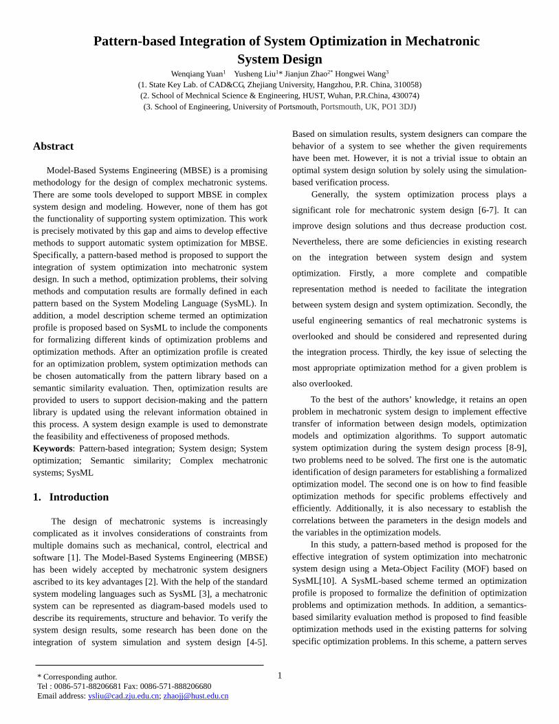
necessary to describe more details for an optimization problem based on the specification of the elements related to an optimization problem discussed in Section 4.1. To achieve this goal, a stereotype «Problem» is proposed based on the SysML meta-class, and another stereotype, «ProblemInstance», is used to represent the semantics of the related optimization instance. Information structure of the stereotypes is shown in Fig. 3.

Fig. 3. Stereotype for defining an optimization problem.

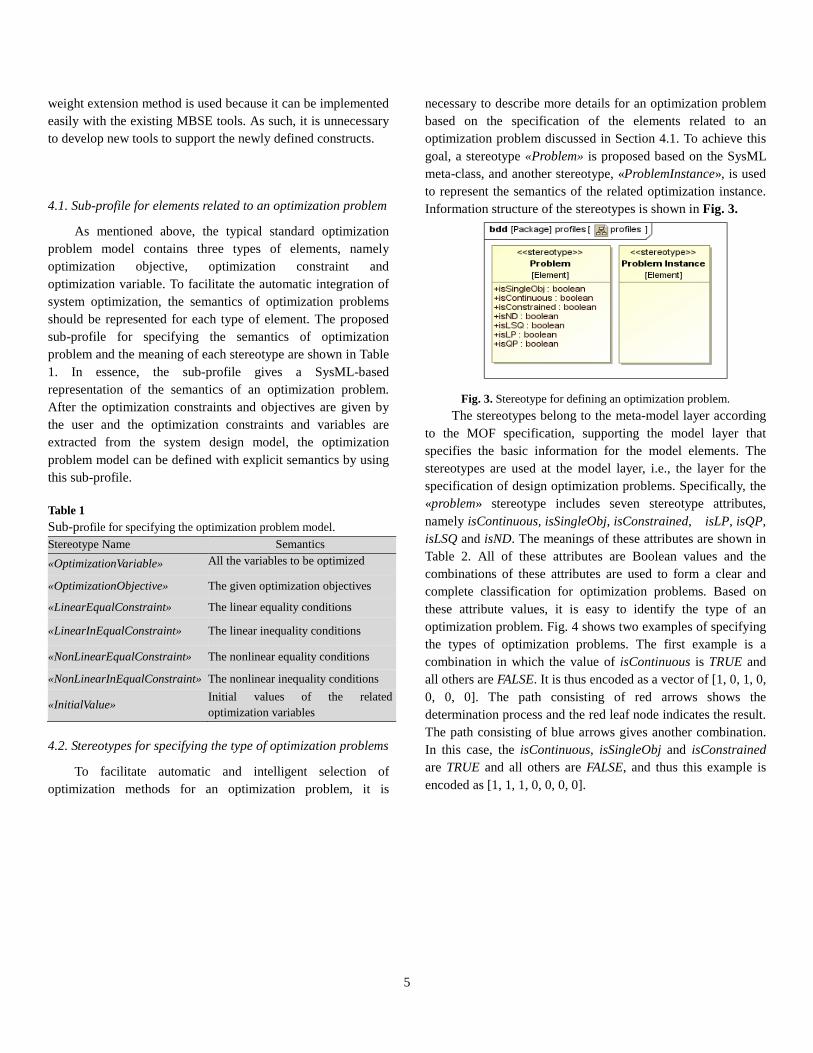
The stereotypes belong to the meta-model layer according to the MOF specification, supporting the model layer that specifies the basic information for the model elements. The stereotypes are used at the model layer, i.e., the layer for the specification of design optimization problems. Specifically, the «problem» stereotype includes seven stereotype attributes, namely isContinuous, isSingleObj, isConstrained, isLP, isQP, isLSQ and isND. The meanings of these attributes are shown in Table 2. All of these attributes are Boolean values and the combinations of these attributes are used to form a clear and complete classification for optimization problems. Based on these attribute values, it is easy to identify the type of an optimization problem. Fig. 4 shows two examples of specifying the types of optimization problems. The first example is a combination in which the value of isContinuous is TRUE and all others are FALSE. It is thus encoded as a vector of [1, 0, 1, 0, 0, 0, 0]. The path consisting of red arrows shows the determination process and the red leaf node indicates the result. The path consisting of blue arrows gives another combination. In this case, the isContinuous, isSingleObj and isConstrained are TRUE and all others are FALSE, and thus this example is encoded as [1, 1, 1, 0, 0, 0, 0].

5

Fig. 4. Examples of different types of optimization problems.

Table 2 Meanings of the stereotype attributes. Attribute Meaning

isSingleObj Indicates if it is a single- or multiple-objective optimization problem

isContinuous Indicates if it is a discrete or continuous problem

isConstrained Indicates whether it is a constrained problem isND Indicates if it is a non-differentiable problem IsLSQ Indicates whether it is a linear square quadratic

problem IsLP Indicates whether it is a linear programming

problem IsQP Indicates whether it is a quadratic programming

problem

To further illustrate the defined stereotypes in this part and the following sections, the inverted pendulum system is used as an example since it is a simple but classical mechatronic product. To keep the inverted pendulum upright, a motor is applied to move the cart back and forth horizontally. This problem aims to achieve two objectives, namely motion range of the inverted pendulum and energy cost of the motor. As a consequence, the value of isSingleObj is FALSE. Continuous variables of the rod length and motor voltage are considered and thus the value of isContinuous is TRUE. Two constraints are also considered: one is to restrict the electricity capacity and another is for keeping the dynamical equivalence of the pendulum. Thus, the value of isConstrained is TRUE. The values of another four tags isLP, isQP, isLSQ and isND are FALSE. On this basis, a continuous constrained multi-objective optimization problem can be constructed, with the corresponding tag values [1, 0,1, 0, 0, 0, 0].

Fig. 5. Inverted pendulum system.

4.3. Engineering semantics description in the pattern

The semantic description of mechatronic systems in the pattern is quite important for the selection of effective and efficient optimization algorithms. In this work, an ontology-based method is developed by extending the general optimization ontology developed by P. Witherell et al. [27].

The basic elements in the optimization ontology are firstly extended. Additionally, mechatronic systems often contain components from multiple domains such as mechanical, electrical, thermal and hydraulic. Developing a complete definition of the mechatronic system semantics is beyond the scope of this paper. As an example, a part of the mechanical-related extended optimization model classes are tabulated in Table 3 [30-32]. It is noteworthy that the same terms in Table 3 can be used as either a variable, constraint or objective function according to specific requirements. It can be seen from Table 3 that the mechanical-related mechatronic semantics used in this study are classified into four types: mechanism kinematics, mechanism dynamics, dynamical performance and structure and shape parameters. For each of these different types, there are various terms that are used to further differentiate the mechatronic system semantics. Other terms can be added for

6

the related types according to their semantics. Each term has one corresponding number. Again, the emphasis of this work is not to develop a complete ontology for mechatronic systems but to develop an effective ontology-based scheme to describe the engineering semantics in mechatronic systems design and optimization.

Table 3

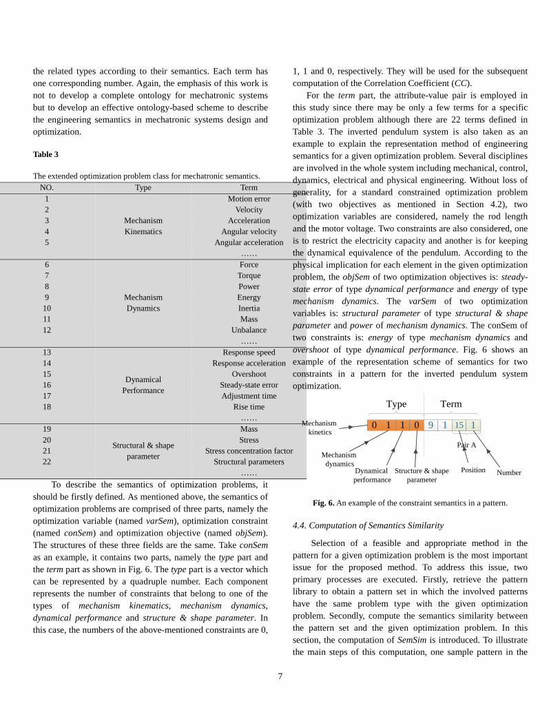
The extended optimization problem class for mechatronic semantics. NO. Type Term

1

Mechanism Kinematics

Motion error 2 Velocity 3 Acceleration 4 Angular velocity 5 Angular acceleration ……

6

Mechanism Dynamics

Force 7 Torque 8 Power 9 Energy

10 Inertia 11 Mass 12 Unbalance

…… 13

Dynamical Performance

Response speed 14 Response acceleration 15 Overshoot 16 Steady-state error 17 Adjustment time 18 Rise time

…… 19

Structural & shape parameter

Mass 20 Stress 21 Stress concentration factor 22 Structural parameters

…… To describe the semantics of optimization problems, it

should be firstly defined. As mentioned above, the semantics of optimization problems are comprised of three parts, namely the optimization variable (named varSem), optimization constraint (named conSem) and optimization objective (named objSem). The structures of these three fields are the same. Take conSem as an example, it contains two parts, namely the type part and the term part as shown in Fig. 6. The type part is a vector which can be represented by a quadruple number. Each component represents the number of constraints that belong to one of the types of mechanism kinematics, mechanism dynamics, dynamical performance and structure & shape parameter. In this case, the numbers of the above-mentioned constraints are 0,

1, 1 and 0, respectively. They will be used for the subsequent computation of the Correlation Coefficient (CC).

For the term part, the attribute-value pair is employed in this study since there may be only a few terms for a specific optimization problem although there are 22 terms defined in Table 3. The inverted pendulum system is also taken as an example to explain the representation method of engineering semantics for a given optimization problem. Several disciplines are involved in the whole system including mechanical, control, dynamics, electrical and physical engineering. Without loss of generality, for a standard constrained optimization problem (with two objectives as mentioned in Section 4.2), two optimization variables are considered, namely the rod length and the motor voltage. Two constraints are also considered, one is to restrict the electricity capacity and another is for keeping the dynamical equivalence of the pendulum. According to the physical implication for each element in the given optimization problem, the objSem of two optimization objectives is: steady-state error of type dynamical performance and energy of type mechanism dynamics. The varSem of two optimization variables is: structural parameter of type structural & shape parameter and power of mechanism dynamics. The conSem of two constraints is: energy of type mechanism dynamics and overshoot of type dynamical performance. Fig. 6 shows an example of the representation scheme of semantics for two constraints in a pattern for the inverted pendulum system optimization.

0 1 1 0 9 1 15 1Mechanism kinetics

Mechanism dynamics

Dynamical performance

Structure & shape parameter

Position Number

Type Term

Pair A

Fig. 6. An example of the constraint semantics in a pattern.

4.4. Computation of Semantics Similarity

Selection of a feasible and appropriate method in the pattern for a given optimization problem is the most important issue for the proposed method. To address this issue, two primary processes are executed. Firstly, retrieve the pattern library to obtain a pattern set in which the involved patterns have the same problem type with the given optimization problem. Secondly, compute the semantics similarity between the pattern set and the given optimization problem. In this section, the computation of SemSim is introduced. To illustrate the main steps of this computation, one sample pattern in the

7

pattern set is used (termed the pattern of interest), whose problem description is a similar optimization problem to the inverted pendulum system and has the same type with the given optimization problem. The difference between the given optimization problem and the pattern of interest is that the latter has one more optimization variable (the cart mass whose semantics is the mass of type mechanism dynamics) and one more constraint ( the velocity restriction for the cart whose semantics is the velocity of type mechanism kinematics). The whole process will be described in Section 6. In this study, the ontology-based semantic similarity measure is used [33].

The computation of SemSim consists of two parts: Correlation Coefficient (CC) and Common Part Coefficient (CPC). The former reflects the degree of correlation between the two parts while the latter intuitively reflects their degree of similarity. The calculation of CC is based on the type of semantic information whereas CPC is based on the terms of semantic information described in Table 3.

4.4.1. Computation of CC

As discussed in Section 4.3, the type part of an optimization variable, constraint and objective is a vector of a quadruple number. Each component represents the number of constraints corresponding to the type of mechanism kinematics, mechanism dynamics, dynamical performance and structure & shape parameter, respectively. Therefore, the vector’s length is 12 for the optimization problem of the inverted pendulum system, as shown on the top part of Fig. 7. With regard to the case in Section 4.3, it has 2 optimization variables. The number of optimization variables with the semantics of mechanism kinematics, mechanism dynamics, dynamical performance and structural & shape parameter are 0, 1, 0 and 1, respectively. Similarly, the number of optimization constraints and objectives with various semantics are also specified using this structure. Meanwhile, the bottom part of Fig. 7 shows the semantics vector of the pattern of interest.

0 1 0 1 0 1 1 0 0 1 1 0

Mechanism kinematics

Mechanism dynamics

Dynamical performance

Structural & shape parameter

0 2 0 1 1 1 1 0 0 1 1 0

Given optimization problem of inverted pendulum system

Comparative pattern

Optimizationvariable

Optimizationconstraint

Optimizationobjective

Fig. 7. An example of semantic information for computing CC.

Given two vectors X and Y (with X representing the semantics of the given optimization problem of the inverted

pendulum system and Y representing the semantics stored in the pattern of interest), then CC can be calculated using the following formula:

1

2 2

1 1

( )( )=

( ) ( )

N

i ii

N N

i ii i

X X Y YCC

X X Y Y

=

= =

− −

− −

∑

∑ ∑

(4)

In the above formula, N is the length for both X and Y.

X and Y are the means of X and Y, respectively. It is obvious

that CC is within the interval [-1, 1]. If the value is pretty large,

X and Y are highly correlated and therefore they are quite

similar in terms of semantics. The Person analysis method can

reflect the correlation degree about two vectors well and its

effectiveness has been proved in various studies of this method

[34-35]. Another advantage of the Person analysis method is its

computational simplicity, which is useful especially when the

pattern library is large.

According to the above formula, the computation value of CC for the given optimization problem of the inverted pendulum system and the pattern of interest is 0.72, which means they are highly correlated. This result is logical since just a slight difference exists between them.

4.4.2. Computation of CPC

In Table 3, each type may contain several terms. For example, there are terms of motion error, velocity, acceleration, angular velocity and angular acceleration for the type of mechanism kinematics. Similar to CC, assume that vectors X and Y represent the semantics information of the given optimization problem and the pattern of interest, respectively, then CPC can be calculated as follows:

( , )( , )

CT X YCPCTT X Y

= (5)

( , )CT X Y represents the number of common terms of X and Y while ( , )TT X Y represents the number of total terms of X and Y. This metric addresses the term part of the semantics and can directly reflect the common parts of two vectors in terms of percentage. Different from CC, CPC can measure similarity with a finer granularity. Moreover, its computation process is quite simple and efficient. With regard to this example, CT is 6 and TT is 14, CPC is 0.43. SemSim is the sum of CC and CPC. Therefore, the SemSim value is 1.15 for this

8

example. For each retrieved pattern, the corresponding SemSim is computed and a SemSim set is thus obtained. Finally, the SemSim set is normalized and ranked in a descending order in terms of the SemSim value.

4.5. Process of formulating a system optimization problem model based on design model

The integration of system optimization into mechatronic system design requires the formulation of a formal optimization problem model based on the system design model. The algorithm for the formulation of an optimization problem is described as follows: (1) Extract the model blocks of system components that

contain the semantics information needed for formulating an optimization problem. These components’ attributes are obtained, and then the extracted design information is transferred to the optimization process. In addition, the constraints are also extracted from the system design model if they are specified as well.

(2) Select the appropriate attributes from the various system components as the optimization variables according to specific design optimization requirements.

(3) Specify the optimization constraints and the optimization objectives based on the defined optimization variables. Both linear and nonlinear constraints are specified based on the physical rules embodied by a mechatronic system. The type of the optimization problem can be uniquely determined according to the specification of optimization conditions and objectives.

(4) Determine the mechatronic system semantics based on the extracted design information by using the semantic information shown in Table 1. The optimization variables, optimization constraints and optimization objectives specified in Step 3 are extracted automatically. For each element, its type is determined first. Then, its corresponding term is also determined for the selected type. The mechatronic system semantics plays an important role in the construction of the optimization problem model since they are used to retrieve the most feasible patterns from the pattern library.

Specify the initial states of the optimization problem in the form of a vector that contains all the optimization variables. In some cases, this step is not required and default values can be given.

5. Sub-profile of optimization methods

Once the sub-profile for optimization problems is established, the next step is to formalize the description of optimization methods. This description will facilitate the selection of feasible optimization methods for a given optimization problem. Selection of feasible methods for an optimization problem means that they can solve the given problem effectively and efficiently. Thus, a pattern would only be feasible if there is at least one feasible method within its description.

5.1. Sub-profile for optimization methods

The information structure of the optimization methods sub-profile is shown in Fig. 8. The optimization method specification contains five items, namely a method name, a method ID, an ‘input part’ which represents an input model, a ‘parameter part’ which represents a parameter model and a ‘result part’ which represents a return model. Specifically, the input model defines the input specification of the optimization problem model. The type of this specification is Set since it may contain many items as introduced in Section 4. The return model reflects the return specification of an optimization method. Certain items are also defined such as the result name, result type, error name and error type. The error item is a flag for an optimization method to indicate specific information such as warnings.

The parameter model defines the parameter specification of a specific optimization method and includes three fields: the name, the type and the value interval. In particular, the value interval of one parameter can be either an interval or just a numerical value. The parameter model is referenced by the input model and the return model and thus the parameters in these models must also be formally defined.

9

Fig. 8. The optimization method profile.

In this study, certain stereotypes are defined to express the relationships between different methods. The common part of a stereotype is used to record the attribute of the common item number, which is the same in different methods. Similarly, the specific part of a stereotype is used to record the attribute of the specific item number.

The data types used in the definition of parameters are shown in Fig. 9. The GeneralForm is associated with the String primitive type and is inherited by the Vector type and the Matrix type. This means it is essentially a String and can be expanded to many different forms. The type of a parameter can be a Vector or a Matrix depending on the specific problem where the parameter is defined.

Fig. 9. The data types used in the method definition.

5.2. Rrepresentation of an optimization method using the sub-profile

To facilitate the automatic selection of feasible optimization methods for a given system optimization problem, the optimization method concerned must also be formally

represented. To the best of the authors’ knowledge, there is no uniform classification for various optimization methods. Some of them are general-purpose and can be used for most optimization problems while the others are problem-specific. The classification method used in [25] is adopted in this study.

Furthermore, there are various optimization methods for each problem-specific category. The category for the constrained methods is represented in Fig. 10. Each block represents one specific method according to the sub-profile described in Section 5.1. In this case, the constrained block is stereotyped with a common part whose item number is assigned the value 3, which indicates all the methods inherited from the constrained method have these three items: (1) the vector x for representing the optimization variables; (2) the real variable minf for representing the return value; and (3) the item GeneralForm, f, for representing the optimization objective, which can be a vector, a matrix or a string. For the block stereotyped with the specific part, this kind of method contains not only the inherited items but also several specific items. For example, the Outside Point Penalty Function method contains three common items x, minf and f and five specific items: the constraint matrix A and vector b, the initial value of the penalty parameter c1, the ratio coefficient of the penalty parameter p and the initial point x0.

10

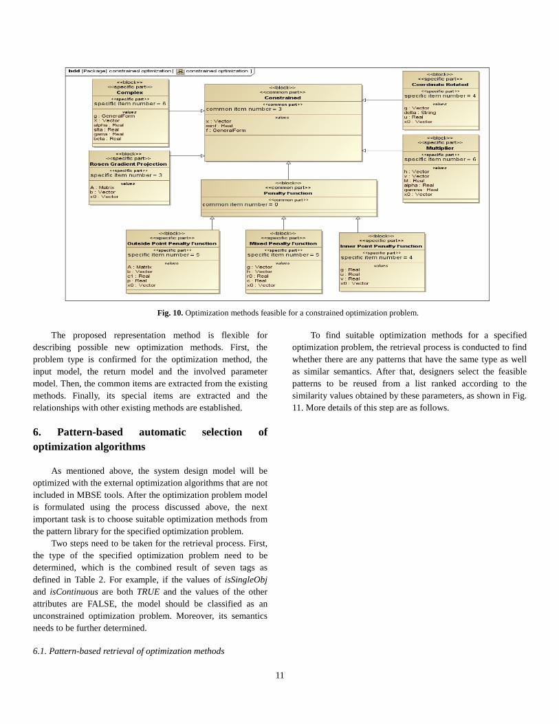
Fig. 10. Optimization methods feasible for a constrained optimization problem.

The proposed representation method is flexible for

describing possible new optimization methods. First, the problem type is confirmed for the optimization method, the input model, the return model and the involved parameter model. Then, the common items are extracted from the existing methods. Finally, its special items are extracted and the relationships with other existing methods are established.

6. Pattern-based automatic selection of optimization algorithms

As mentioned above, the system design model will be optimized with the external optimization algorithms that are not included in MBSE tools. After the optimization problem model is formulated using the process discussed above, the next important task is to choose suitable optimization methods from the pattern library for the specified optimization problem.

Two steps need to be taken for the retrieval process. First, the type of the specified optimization problem need to be determined, which is the combined result of seven tags as defined in Table 2. For example, if the values of isSingleObj and isContinuous are both TRUE and the values of the other attributes are FALSE, the model should be classified as an unconstrained optimization problem. Moreover, its semantics needs to be further determined.

6.1. Pattern-based retrieval of optimization methods

To find suitable optimization methods for a specified optimization problem, the retrieval process is conducted to find whether there are any patterns that have the same type as well as similar semantics. After that, designers select the feasible patterns to be reused from a list ranked according to the similarity values obtained by these parameters, as shown in Fig. 11. More details of this step are as follows.

11

The specified optimization

problem

Type of specified optimization

problem

Pattern library

Semantics of specified

optimization problem

Semantics of one pattern

Type of one pattern

Calculate SemSim

Same or last

pattern?

Is the last pattern?

Feasible patterns

Corresponding SemSim

No

No

Yes

Yes

Input

The type determination

process

The semantics determination

process

OutputFeasible patterns

Fig. 11. The pattern-based retrieval process.

(1) Determine the type of the specified optimization problem and the type of one pattern from the pattern library.

(2) Compare the type of the specified optimization problem and the type of the current pattern. If they are the same, the current pattern is considered as a feasible pattern and Step 3 will be executed. If no feasible pattern exists, designers have to select the optimization methods according to their experience. In this case, a new pattern is created and then added to the pattern library.

(3) Extract the semantics of the current pattern and analyze its meaning to classify the type for each element using the information in Table 3.

(4) Calculate the semantic similarity (SemSim) between the semantics of the specified optimization problem and those of some feasible patterns from the library. The detailed calculation process will be described in Section 6.2.

(5) Repeat Steps 2 and 3 for each pattern in the pattern library and sort the patterns according to the SemSim values. The output of this process then contains the ranked patterns and their corresponding SemSim values.

6.2. The solving of optimization problems

After some feasible patterns are obtained, one appropriate pattern can be chosen based on the SemSim value and

optimization performance, the corresponding optimization method stored in the chosen pattern can be applied to the optimization problem. The following steps are taken to solve the given optimization problem: (1) Specify the initial values of parameters of the selected

optimization method; (2) Specify the initial state for the optimization problem; (3) Run the external optimization algorithm and obtain

optimization results. Then, update the system design model based on the optimization results.

6.3. Maintenance of the pattern library

After an optimization problem is solved using a particular optimization method, the pattern library should be updated and maintained. If no feasible patterns are found in the pattern library for the given optimization problem, an appropriate optimization method will be chosen by designers to solve the optimization problem. In this case, a pattern with new type of optimization problem is then generated and inserted into the pattern library. If some feasible patterns are found in the pattern library, the optimization problem will be solved by using the optimization method in the feasible patterns and thus a pattern with the same type but different parameter values in other fields will also be added to the pattern library.

7. Implementation and a case study

The proposed methods and algorithms have been implemented based on the MagicDraw 16.5 MBSE tool, MATLAB and MySQL. Specifically, the APIs of MagicDraw 16.5 are used to implement the necessary functions. MATLAB is used to run the optimization methods, and the MySQL database management system is used to store the pattern library.

7.1. A system design example

In this study, a real-world mechatronic design problem is used to test the proposed approach. In De Silva et al. [36], a Continuously Variable Transmission (CVT) is presented in which transmission ratio can be continuously changed within an established range and thereby produces smooth outputs. This pinion-rack CVT is composed of many conventional mechanical elements such as a gear pinion, one circular cam, two pairs of racks and two sliders. The pinion-rack CVT changes its transmission ratio when the distance between the input and output rotation axes is changed. This distance is called "offset" and will be denoted as "e". Inside the CVT, an offset mechanism is integrated. Fig. 12 shows the CVT prototype used in this study.

12

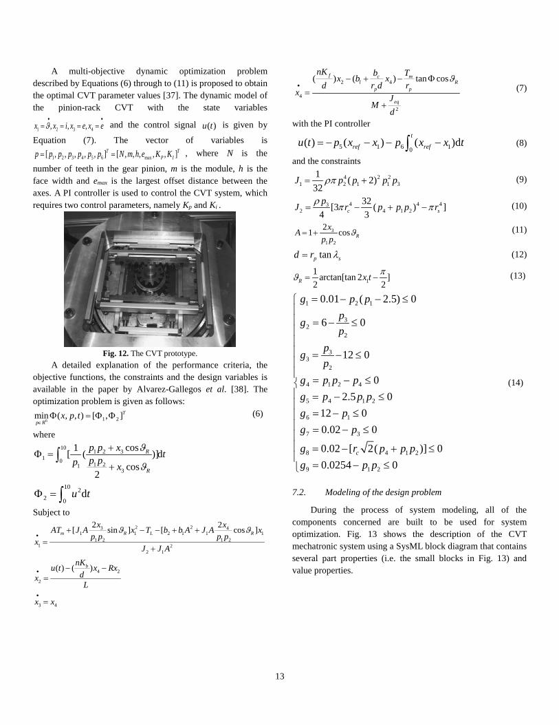
A multi-objective dynamic optimization problem described by Equations (6) through to (11) is proposed to obtain the optimal CVT parameter values [37]. The dynamic model of the pinion-rack CVT with the state variables

1 2 3 4, , ,x x i x e x eϑ• •

= = = = and the control signal ( )u t is given by

Equation (7). The vector of variables is

1 2 3 4 5 6 max[ , , , , , ] [ , , , , , ]T TP Ip p p p p p p N m h e K K= = , where N is the

number of teeth in the gear pinion, m is the module, h is the face width and emax is the largest offset distance between the axes. A PI controller is used to control the CVT system, which requires two control parameters, namely Kp and Ki .

Fig. 12. The CVT prototype.

A detailed explanation of the performance criteria, the objective functions, the constraints and the design variables is available in the paper by Alvarez-Gallegos et al. [38]. The optimization problem is given as follows:

6 1 2min ( , , ) [ , ]T

p Rx p t

∈Φ = Φ Φ (6)

where 10 1 2 3

1 0 1 213

cos1[ ( )]dcos

2

R

R

p p x tp pp x

ϑ

ϑ

+Φ =

+∫

10 22 0

du tΦ = ∫

Subject to 2 23 4

1 1 2 1 1 11 2 1 2

1 22 1

2 2[ sin ] [ cos ]m R L Rx xAT J A x T b b A J A x

p p p pxJ J A

ϑ ϑ•

+ − − + +=

+

4 2

2

( ) ( )bnKu t x RxdxL

• − −=

3 4x x•

=

2 4

4

2

( ) ( ) tan cosf c ml R

p p

eq

nK b Tx b xd r d r

x JM

d

ϑ•

− + − Φ=

+

(7)

with the PI controller

5 1 6 10( ) ( ) ( )d

t

ref refu t p x x p x x t= − − − −∫ (8)

and the constraints

4 2 21 2 1 1 3

1 ( 2)32

J p p p pρπ= + (9)

4 4 432 4 1 2

32[3 ( ) ]4 3c spJ r p p p rρ π π= − + − (10)

3

1 2

21 cos RxA

p pϑ= + (11)

tanp sd r λ= (12)

11 arctan[tan 2 ]2 2R x t πϑ = − (13)

1 2 1

32

2

33

2

4 1 2 4

5 4 1 2

6 1

7 3

8 4 1 2

9 1 2

0.01 ( 2.5) 0

6 0

12 0

02.5 0

12 00.02 0

0.02 [ 2( )] 00.0254 0

c

g p ppgp

pgp

g p p pg p p pg pg p

g r p p pg p p

= − − ≤ = − ≤ = − ≤ = − ≤ = − ≤

= − ≤ = − ≤ = − + ≤

= − ≤

(14)

7.2. Modeling of the design problem

During the process of system modeling, all of the components concerned are built to be used for system optimization. Fig. 13 shows the description of the CVT mechatronic system using a SysML block diagram that contains several part properties (i.e. the small blocks in Fig. 13) and value properties.

13

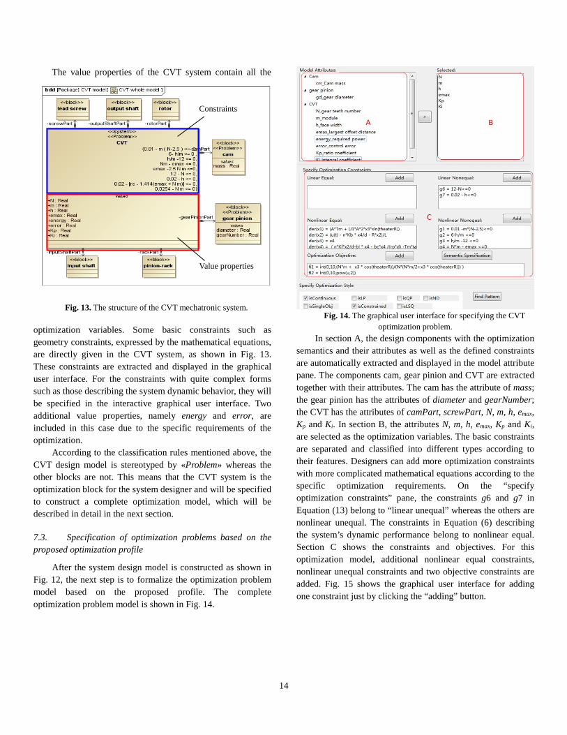
The value properties of the CVT system contain all the

optimization variables. Some basic constraints such as geometry constraints, expressed by the mathematical equations, are directly given in the CVT system, as shown in Fig. 13. These constraints are extracted and displayed in the graphical user interface. For the constraints with quite complex forms such as those describing the system dynamic behavior, they will be specified in the interactive graphical user interface. Two additional value properties, namely energy and error, are included in this case due to the specific requirements of the optimization.

According to the classification rules mentioned above, the CVT design model is stereotyped by «Problem» whereas the other blocks are not. This means that the CVT system is the optimization block for the system designer and will be specified to construct a complete optimization model, which will be described in detail in the next section.

7.3. Specification of optimization problems based on the proposed optimization profile

After the system design model is constructed as shown in Fig. 12, the next step is to formalize the optimization problem model based on the proposed profile. The complete optimization problem model is shown in Fig. 14.

Fig. 14. The graphical user interface for specifying the CVT

optimization problem. In section A, the design components with the optimization

semantics and their attributes as well as the defined constraints are automatically extracted and displayed in the model attribute pane. The components cam, gear pinion and CVT are extracted together with their attributes. The cam has the attribute of mass; the gear pinion has the attributes of diameter and gearNumber; the CVT has the attributes of camPart, screwPart, N, m, h, emax, Kp and Ki. In section B, the attributes N, m, h, emax, Kp and Ki, are selected as the optimization variables. The basic constraints are separated and classified into different types according to their features. Designers can add more optimization constraints with more complicated mathematical equations according to the specific optimization requirements. On the “specify optimization constraints” pane, the constraints g6 and g7 in Equation (13) belong to “linear unequal” whereas the others are nonlinear unequal. The constraints in Equation (6) describing the system’s dynamic performance belong to nonlinear equal. Section C shows the constraints and objectives. For this optimization model, additional nonlinear equal constraints, nonlinear unequal constraints and two objective constraints are added. Fig. 15 shows the graphical user interface for adding one constraint just by clicking the “adding” button.

Fig. 13. The structure of the CVT mechatronic system.

Value properties

Constraints

14

Fig. 15. The interface for adding a new constraint.

7.4. Specification of mechatronic semantics

To specify the mechatronic semantics for the optimization model, a new user interface as shown in Fig. 16 is provided to the designers when they click the “semantic specification” button in Fig. 14.

Fig. 16. Specification of mechatronic semantics.

On the variable semantics pane, the optimization variables can be specified by assigning a domain value. In this case, h and emax belong to the mechanical system while Kp and Ki

belong to the controller. On the “constraints semantics” pane, the optimization

constraints can be specified by first determining their classifiers and then their detailed semantic information. Specifically, the constraints in Equation (14) are classified into structural & shape parameters and their semantic information belongs to inertia. For the constraints in Equation (7), they are classified into dynamic performance and are thus specified with the mechatronic semantics of torque, power and force.

On the “objectives semantics” pane, the first constraint in Equation (5) is classified as mechanism kinematics and

response speed is specified as its semantic information while the second constraint is dynamical performance and steady-state error is specified as its semantic information.

7.5. Solving of optimization problem based on pattern

To evaluate the problem solving process, the following three cases are considered. First, assume that the given optimization problem is new and thus there is no feasible pattern in the pattern library with the same type. In this case, designers have to select optimization methods for this new optimization problem. The second case is that feasible patterns can be found for the given optimization problem. In this case it will be solved with the support of pattern-based selection of optimization methods. The third case is similar to the second one except that different initial instances are considered. For each of the three cases a new pattern will be created and added into the pattern library.

The tag attributes of the «Problem» stereotype are displayed in the pane in the form of a series of checking button. After the mechatronic semantics is specified, the type of the optimization problem should be specified by clicking those checking buttons.

After the “find pattern” button is clicked, the process of pattern retrieval is started. Designers then can compare the records of the pattern library and their performance data to make decisions. If no suitable patterns have been found, the optimization methods corresponding to this optimization type are listed. One of the optimization methods would be used to solve the optimization problem.

To illustrate the three cases mentioned above, three optimization instances of the CVT system with different configurations are shown in Fig. 17. Specifically, the energy and error value properties are the candidates of the optimization objectives and these instances correspond to different optimization problems specified before. To illustrate the pattern-based selection method, over one hundred patterns have been created and stored in the library, as shown in Fig. 18. It can be seen that each pattern has a full set of fields (with different values) including several optimization problems with different types and optimization methods with different features and configurations. The type information can be inferred by the value of the tag field.

15

Fig. 17. Three CVT instances with different initial values.

Fig. 18. Examples of patterns in the library.

7.5.1. Optimization problems without feasible patterns

The first case is a constrained optimization problem with a single objective for which instance A is used. In instance A, the tag attribute combination is as follows: isContinuous, isSingleObj and isConstrained are TRUE and the others are FALSE. In addition, its tag attribute in the pattern library is [1, 1, 1, 0, 0, 0, 0]. Only the first objective remains after the optimization problem is specified and six attributes N, m, h, emax, Kp and Ki are selected as the optimization variables. All the constraint equations are selected when the optimization constraints are added. After these elements are determined, their semantic specifications will be completed.

The result of the selection process is that no feasible pattern will be obtained since there is no such a pattern that has exactly the same problem type as this case. Therefore, the optimization methods corresponding to this type presented in Section 6 are found and listed, as shown in Fig. 19.

In this case, the inner point penalty function is selected to solve the specified optimization problem and it is configured firstly by specifying the penalty factor u as 8.0 and the contraction factor v as 0.5, as shown in Fig. 20. Then, the specified optimization problem is solved and a new pattern is created and the related information such as the type and detailed semantic information, the optimization method and its optimization performance is saved.

Fig. 19. Methods defined in the profile for constrained problems.

16

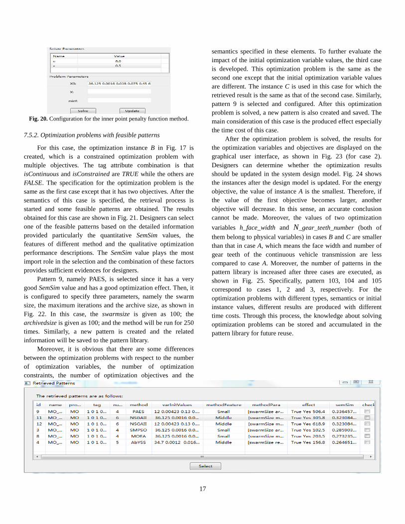
Fig. 20. Configuration for the inner point penalty function method.

7.5.2. Optimization problems with feasible patterns

For this case, the optimization instance B in Fig. 17 is created, which is a constrained optimization problem with multiple objectives. The tag attribute combination is that isContinuous and isConstrained are TRUE while the others are FALSE. The specification for the optimization problem is the same as the first case except that it has two objectives. After the semantics of this case is specified, the retrieval process is started and some feasible patterns are obtained. The results obtained for this case are shown in Fig. 21. Designers can select one of the feasible patterns based on the detailed information provided particularly the quantitative SemSim values, the features of different method and the qualitative optimization performance descriptions. The SemSim value plays the most import role in the selection and the combination of these factors provides sufficient evidences for designers.

Pattern 9, namely PAES, is selected since it has a very good SemSim value and has a good optimization effect. Then, it is configured to specify three parameters, namely the swarm size, the maximum iterations and the archive size, as shown in Fig. 22. In this case, the swarmsize is given as 100; the archivedsize is given as 100; and the method will be run for 250 times. Similarly, a new pattern is created and the related information will be saved to the pattern library.

Moreover, it is obvious that there are some differences between the optimization problems with respect to the number of optimization variables, the number of optimization constraints, the number of optimization objectives and the

semantics specified in these elements. To further evaluate the impact of the initial optimization variable values, the third case is developed. This optimization problem is the same as the second one except that the initial optimization variable values are different. The instance C is used in this case for which the retrieved result is the same as that of the second case. Similarly, pattern 9 is selected and configured. After this optimization problem is solved, a new pattern is also created and saved. The main consideration of this case is the produced effect especially the time cost of this case.

After the optimization problem is solved, the results for the optimization variables and objectives are displayed on the graphical user interface, as shown in Fig. 23 (for case 2). Designers can determine whether the optimization results should be updated in the system design model. Fig. 24 shows the instances after the design model is updated. For the energy objective, the value of instance A is the smallest. Therefore, if the value of the first objective becomes larger, another objective will decrease. In this sense, an accurate conclusion cannot be made. Moreover, the values of two optimization variables h_face_width and N_gear_teeth_number (both of them belong to physical variables) in cases B and C are smaller than that in case A, which means the face width and number of gear teeth of the continuous vehicle transmission are less compared to case A. Moreover, the number of patterns in the pattern library is increased after three cases are executed, as shown in Fig. 25. Specifically, pattern 103, 104 and 105 correspond to cases 1, 2 and 3, respectively. For the optimization problems with different types, semantics or initial instance values, different results are produced with different time costs. Through this process, the knowledge about solving optimization problems can be stored and accumulated in the pattern library for future reuse.

17

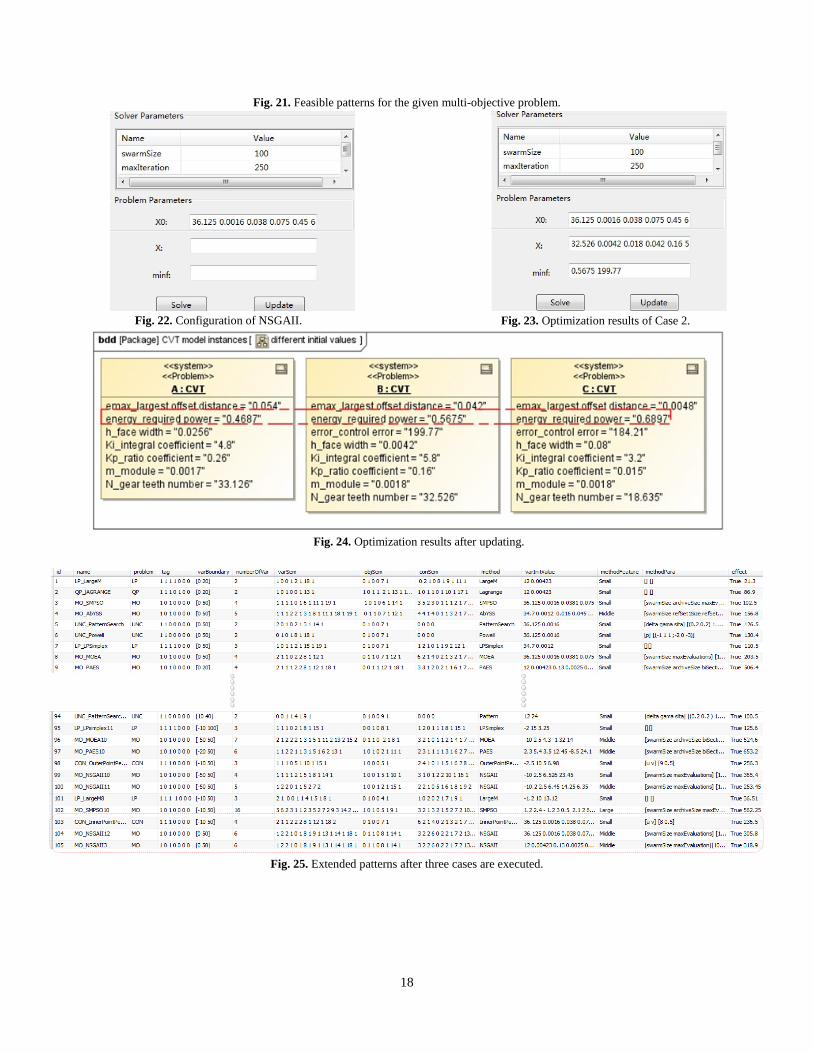
Fig. 21. Feasible patterns for the given multi-objective problem.

Fig. 22. Configuration of NSGAII.

Fig. 23. Optimization results of Case 2.

Fig. 24. Optimization results after updating.

Fig. 25. Extended patterns after three cases are executed.

18

8. Conclusions and future work

In this paper, a pattern-based method for the integration of system optimization into mechatronic system design is proposed based on the SysML extension mechanism. The whole process is demonstrated and the proposed method is evaluated based on the CVT example. The main contributions of this work are summarized as follows: (1) The pattern concept is introduced to capture and reuse the

knowledge about understanding optimization problems and selecting optimization methods by exploiting the semantic information of complex mechatronic systems. The fields in the pattern structure are defined and described in detail.

(2) A new profile for complex system optimization is proposed to realize the automatic integration of system optimization into complex mechatronic system design based on an extension of SysML. It includes three sub-profiles for describing optimization problems, engineering semantics and optimization methods, respectively. Using these sub-profiles, rich mechatronic engineering semantics can be described and utilized in the formulation of optimization problems.

(3) A semantics-based similarity evaluation method is proposed for retrieving and selecting feasible optimization methods from the pattern library. Two parameters, i.e., the correlation coefficient and the common part coefficient are proposed to measure the semantic distance between two optimization problems. The computation of semantics similarity is shown using an example of the inverted pendulum system. In addition, the whole reasoning process is also demonstrated in the experiment section. The case study has demonstrated the effectiveness of the

proposed method. All the key tasks such as the extraction of design information from the system design model, the construction of the complete optimization model and the retrieval of feasible optimization methods are completed satisfactorily. However, it is still in an early stage and there are also some limitations in this work. The mechatronic semantics defined in this work is still not comprehensive. It contains only partial information of the semantics specific to mechanical engineering. A complete definition of the semantic information for mechatronic systems will be considered in our future work. Meanwhile, there is still no unique classification standard for different types of optimization problems and various optimization methods. Another area that should be improved and refined is the completeness of the mechatronic ontology and the semantics-based similarity evaluation. More guidelines should be considered in the selection of optimization methods

and similarity evaluation. In addition, the scale of the pattern library is still not large but the number of patterns keeps increasing as more and more case studies are completed.

Acknowledgment The authors appreciate the supports from the National

Science Foundation of China (Grant Nos. 61572427 and 61370182), the National Key Technology Support Program (Grant No. 2014BAD04B00) and the Key Project of Science and Technology of Zhejiang Province (Grant No. 2014C01052).

References

[1] Michelle B, David H. System design: new product development for mechatronic, Aberdeen Group, Benchmark report. 2008.

[2] Fisher J, Model-Based Systems Engineering: A New Paradigm. INCOSE Insight. 1998;1 (3): 3-16.

[3] Object Management Group (OMG). Systems Modeling Language specification. <http.//www.omg.org/spec/ SysML/1.2/PDF>, 2014 (accessed 12.27.2014).

[4] Vanderperren Y, Dehaene W. From UML/SysML to Matlab/Simulink: current state and future perspectives. Proc. of design, automation and test in Europe (DATE). Munich, Germany, Mar. 6-10. 2006.

[5] SysML-Modelica integration working group, SysML Modelica transformation specification version 1.0, 2010. <http://www.omgwiki.org/OMGSysML/doku.php?id=sysml-modelica:sysml_and_modelica_integration>, 2014 (accessed 12.30.2014).

[6] Kaveh A, Laknejadi K. A new multi-swarm multi-objective optimization method for structural design. Advances in Engineering Software. 2013; 58:54-69.

[7] Gustavo RZ, Antonio JN, Juan JD. Integrating a multi-objective optimization framework into a structural design software. Advances in Engineering Software. 2014; 76:161-170.

[8] Dentsoras JA. Problem-dependent search for optimal parameter instantiation order in design spaces. ADV ENG INFORM. 2009;23 (4): 474-482.

[9] Geyer P. Component-oriented decomposition for multidisciplinary design optimization in building design. ADV ENG INFORM.2009; 23 (1): 12-31.

[10] Meta-object Facility. < http://www.omg.org/mof/>, 2015 (accessed 1.27.2015).

[11] Cagan J, Campbell MI, Finger S. A framework for computational design synthesis--model and applications. Journal of computing and information science in

19

engineering. 2005 ; 5:171-181. [12] Helms B, Shea K, Hoisl F. A framework for

computational design synthesis based on graph-Grammars and function-behavior-structure. ASME IDETC/CIE’2009, San Diego, California, USA, Aug. 30 – Sept. 2. 2009.

[13] Alber R, Rudolph S A generic approach for engineering design grammars. AAAI Technical report SS-03-02. 2008.

[14] Sim YW, Crowder R, Robinson M. An agent-based approach to modeling integrated product teams undertaking a design activity. ASME IDETC/CIE’2009, San Diego, California, USA, Aug. 30 – Sept. 2, 2009.

[15] DF J, SK M. Multiobjective meta-heuristics: an overview of the current state-of-the-art. Eur J. Oper. Res. 2002; 137(1):1-9.

[16] Coello C. A comprehensive survey of evolutionary multiobjective optimization techniques. Knowl Inform Syst. 1999; 1(3):169-308.

[17] Nomagic. <http://www.nomagic.com/text.php>, 2015 (accessed 1.27.2015).

[18] Min BI, Kerzhner AA, Paredis CJJ. Process integration and design optimization for model-based systems engineering with SysML. IDETC/CIE 2011.

[19] ModelCenter. <http://www.phoenix-int.com/software/ phx_modelcenter. php.>, 2015 (accessed 1.27.2015).

[20] Vanderperren Y, Dehaene W. From UML/SysML to Matlab/Simulink : current state and future perspectives. Proc. of design, automation and test in Europe (DATE). Iunich, Germany, Mar. 6-10. 2006.

[21] Turki S, Soriano T. A SysML extension for bond graphs support. 5th Int. Conf. on technology and automation, Thessaloniki, Greese, Oct. 15-16, 2005.K. Ulrich, S. Eppinger. Product Design and Development. McGraw-Hill, New York. 1995.

[22] Pop A, Akhvlediani D, Fritzson P. Towards unified systems modeling with the ModelicaML UML profile. International workshop on Equation-Based Object-Oriented Languages and Tools, Linköping University Electronic Press, Berlin, Germany. 2007.

[23] Modelica Association. Modelica language specification, <htttp://www.modelica.org/documents/ModelicaSpec31.pdf.>, 2009 (accessed 12.5.2009).

[24] Unified modeling language. <http://www.uml.org/>, 2014 (accessed 12.27.2014).

[25] Johnson TA, Paredis CJJ, Burkhart R. Modeling continuous system dynamics in SysML. in ASME International Mechanical Engineering Congress and

Exposition ASME, Seattle, WA. 2007. [26] Qamar A, Torngren M, Wikander J. Integrating Multi-

Domain Models for the Design and Development of Mechatronic Systems. 7th European Systems Engineering Conference EuSEC, Stokholm. 2010.

[27] Witherell P, Krishnamurty S, Grosse IR. Ontologies for Supporting Engineering Design Optimization. Journal of Computing and Information Science in Engineering. 2007; 7:141- 150.

[28] Gong L, Wang ZL. Mastering Matlab optimality computation, second ed., Publishing house of electronics industry, Beijing. 2012.

[29] Shi WP, Liu YX, Guo SH. Convergence criteria of optimality algorithms.

[30] Yang JH. The kinematics and dynamics of mechanism. Mechanical engineering press, Beijing, China. 1987.

[31] Xu YY. The dynamics of mechanical systems. Mechanical engineering press, Beijing, China. 1990.

[32] Liang DP, Li BL. The dynamic measurement technology of mechanical engineering parameters, Beijing, China. 1995.

[33] Lee W, Shah N. Comparison of Ontology-based Semantic-Similarity Measure. AMIA Symposium Proceedings. 2008.

[34] Kelly HZ, Kernal T, Stuart GS. Correlation and simple linear regression. Radiology. 2003; 227:617-628.

[35] Kenji F, Francis RB, Arthur G. Statistical consistency of kernel canonical correlation analysis. Journal of Machine Learning Research. 2007; 8:361-383.

[36] Silva D, Solejsi M. Kinematic analysis and design of a continuously variable transimission. Mechanism and Machine Theory . 2009; 29(1): 149-167.

[37] Alvarez-Gallegos J, Cruz-Villar C, Portialla-Flores E. Parametric Optimal design of a pinion-rack based continuously variable transmission. In: Proceedings of the 2005 IEEE/ASME International Conference on Advanced Intelligent Mechatronic, Monterey, California, USA. 2005; 899-904.

[38] Alvarez-Gallegos J, Cruz-Villar C, Portilla-Flores E. Evolutionary dynamic optimization of a continuously variable transmission for mechanical efficiency maximization. In: A. Gelbukh, A. de Albornoz, H. Terashima-Marin, MICAI 2005: Advances in Artificial Intelligence, Lectures Notes in Artificial Intelligence, Springer. 2005; 3789: 1093-11

20