patrick t. brandt associate professor - computational...
TRANSCRIPT
RACING HORSES: CONSTRUCTING AND EVALUATING FORECASTS IN
POLITICAL SCIENCE1
Patrick T. BrandtAssociate Professor
School of Economic, Political, and Policy Science, University of Texas, Dallas800 W. Campbell Road, GR31, Dallas, TX 75080-3021
Phone: 972-883-4923, Fax: 972-883-6297, Email: [email protected]
John R. FreemanProfessor
Department of Political Science, University of Minnesota1414 Social Sciences Bldg; 267 19th Ave. South; Mpls, MN 55455
Phone: 612-624-6018, Fax: 612-624-7599, Email: [email protected]
Philip A. SchrodtProfessor
Department of Political Science, Pennsylvania State University227 Pond Laboratory, University Park, PA 16802-6200
Phone: 814-863-8978, Fax: 814-863-8979, Email: [email protected]
1Paper presented at the 28th Summer Meeting of the Society for Political Methodology, Princeton University, July2011. This research is supported by the National Science Foundation, award numbers SES 0921051, SES 0921018,and SES 1004414. We thank Michael D. Ward for comments. The authors are responsible for the paper’s contents.

Brandt, Freeman & Schrodt Racing Horses
1 Introduction
In recent years, political forecasting has become a more common exercise. These forecasts
range from predictions of election outcomes (Campbell 2000, 2010a) to forecasts of political insta-
bility (O’Brien 2010, Goldstone, et al. 2010). They are intended to aid campaign managers, political
observers, policy makers. The analysts who produce them often compare, either implicitly or ex-
plicitly, the performance of their forecasting models to that of competing models. If the model is
successful, they declare it the winner, as if their horse had beaten its competitors in a race.1
Meanwhile, scholars in disciplines as diverse as statistics, meteorology and finance are con-
ducting formal forecasting competitions. Their works illuminate important methodological chal-
lenges such as striking a balance between judgmental and model-based forecasts and choosing
between nonstructural and structural (theory laden) functional forms. These forecasters address
important design issues as well: measuring initial conditions and coping with data vintaging, us-
ing in-sample and out-of-sample data (recursively) in evaluations, and deciding whether and how
to make forecasts across breakpoints. Their exercises use a combination of scoring rules and other
tools—tools that include interval, density, and spatial evaluations of forecasts—and have shown
that a suite of methods is needed to determine which forecasting model is the best performer.
Table 1 summarizes some of these features of meteorological and macroeconomic forecasting in
relation to two kinds of forecasts that are increasingly common in political science.2
Unfortunately, the horse races found in political science are less rigorous than those conducted
in many other disciplines. We generally ignore critical modeling and design issues. Some leading
forecasters in international relations forecasters produce prediction that are “off on time.” That is,
the predictions do not indicate when an event will occur nor how much uncertainty is associated
with the prediction (see Brandt, et al. 2010). In general, political science also uses an antiquated
set of tools to evaluate our point forecasts, typically Mean Absolute Error (MAE) and Root Mean
Squared Error (RMSE). Such point forecasts contain no information about estimation and other
kinds of uncertainty (Tsay and Wallace 2000: 235). Also, metrics like RMSE fail the reliability
criterion (Armstrong and Collopy 1992).
Consider the Political Instability Task Force’s (PITF) claim to outperform a model based on
Fearon and Laitin’s (2003) theory of civil war. Goldstone, et al. (2010) report that its model yields
a higher percentage of correct predictions. But how precise is this percentage? What are the con-
fidence intervals for the PITF and Fearon-Laitin predictions? Is there substantial overlap among
1Campbell (2000) argues that forecasting contributes to political science; Schrodt (2010), basing his argumentson the logical positivists Hempel and Quine, goes further to assert that unless validated by prediction, models, eventhose lovingly structured with elaborate formalisms and references to wizened authorities, are merely “pre-scientific.”
2The interest (advances in) risk management in the 1990s resulted in finance adopting many of the tools used inmeteorology. To keep things more simple in Table 1, we stress the contrasts between meteorological, macroeconomic,and political forecasting. A short but useful history of macroeconomic forecasting can be found in Clements andHendry (1995: Section 1.3) These authors also produce a typology of 216 cases of macroeconomic forecasts, casesdistinguished by such things as whether the forecasting model is or is not claimed to represent the data generatingprocess and whether linearity is or is not assumed.
2
Brandt, Freeman & Schrodt Racing Horses
these confidence intervals? If yes, how do we incorporate this overlap in our evaluation of the two
models? What forecast densities are associated with each model and how do we include an evalu-
ation of these densities in this horse race? The answers to these questions are important because
Diebold et al. (1998) show that if we can find the correct density for the data generating process,
all forecast users (for example policy makers) will prefer to use it regardless of their loss functions.
In general, political scientists have not incorporated, in any systematic way, judgmental ap-
proaches to constructing forecasting models or to modeling important break points (nonlinear-
ities) in political processes. Our forecasting competitions are poorly designed, with ambiguous
or ad hoc guidelines for the choice of training sets, forecast benchmarks, and other design ele-
ments. In addition, forecasters in political science have generally ignored the probabilistic nature
of the forecasts inherent in estimation and evaluation. This is why the southeast corner of Table
1 is blank: the appropriate tools, to our knowledge, have not been applied in our discipline. As
we will demonstrate, because of these shortcomings, we often draw the wrong inferences about
model performance. We often declare the wrong horse victorious.
This paper shows how to improve forecasting in political science. It is divided into five parts.
The next three sections review the issues involved in (2) building a sound forecasting model, (3),
comparing forecasts, and (4), actually judging model performance. Section 4 will also discuss
the value of a new suite of evaluative tools. The tools include the Continuous Rank Probability
Score, Verification Rank Histogram and Sharpness Diagram. Forecasts in international relations
(political instability and conflict early warning) are critically evaluated throughout sections 2, 3
and 4.3
Section 5 of the paper illustrates how to use the new suite of designs and tools to improve
competitions between forecasting models, first in a stylized Monte Carlo analysis and then in a
horse race between conflict early warning models for the China-Taiwan “Cross-Straits” dyad. The
Monte Carlo analyses highlight the pitfalls of relying on point forecasts and conventional metrics
like RMSE to pick winners. The conflict early warning investigation compares the performance
of a collection of time series models including univariate autoregressions (AR) and multiequation
models including Bayesian, and Markov-Switching Bayesian vector autoregressive models (VAR,
BVAR, MS-BVAR models, respectively).
In Section 6 of the paper, our conclusion, we summarize our results and lay the groundwork for
the sequel to this paper, a review of how best to pool models to enhance forecasting (Montgomery
and Nylan 2010; Montgomery, et al. 2011; Geweke and Amisano 2011).
3In the longer version of this paper, available from the authors, we also critically evaluate the election forecastingliterature at the end of parts 2, 3, and 4.
3
Brandt, Freeman & Schrodt Racing Horses
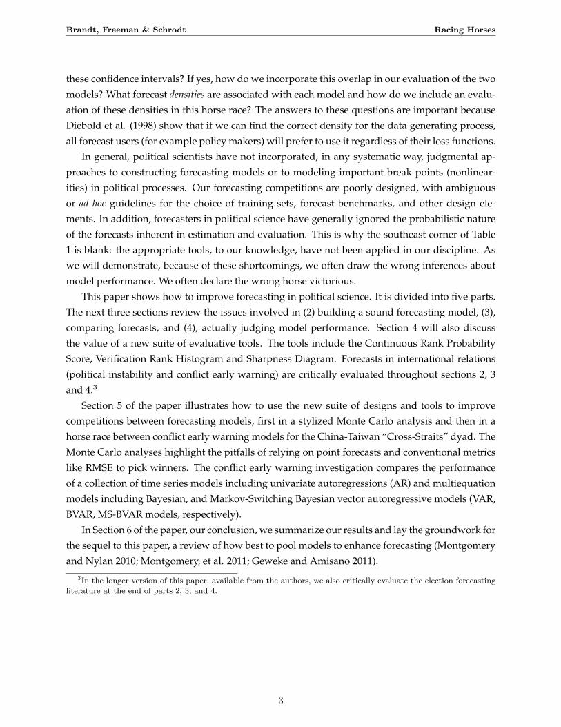
Meteorology Macro- Conflict[Finance] Economic Election Early Warning
2. FORECASTCONSTRUCTION Federal Reserve Cook’s Political
Judgmental vs. Elicita- Green Book Report vs Seats-In- The Call/ICG vs.Model-based tion vs. BVAR Trouble Model PITF
(Non)structural (B)VARvs.NNS, Seats In Trouble vs. PITF vs.Fearon-functional form DSGE Models Referendum Models Laitin Models
Model training Variability Prior Stan-Tradeoff dardzation
3. DESIGNINGMODEL RACES
Measurement- Initial/Boundary Data Datament Conditions Vintaging Vintaging
In-vs.Out-of Sequential Updating; One Election SequentialSample Fixed-Event Design Ahead Ex Ante Ex Post
(Public Domain)
Breakpoints Weather Regimes, Business Realignments ConflictRST Models Cycles Phase Shifts
Benchmark Metrics/ Climatological Thiel’s U2 Thiel’s U2Naive Models NMSE
4. EVALUATIONEvaluation RMSE,MAE MAE,RMSE RMSE ROC
Metrics(Point) MAE Curves
Interval Scoring Fan Charts none noneRules LRcc
Density VRHs,CRPS LPSs,PITs none nonePITs
Spatial MST none none none
Table 1: Selected Features of Forecasting Competitions in Three Disciplines. Numbers of majortopics correspond to section in which they are discussed. Notes. Seats In Trouble and ReferendumModels are the forecasting models proposed by Campbell (2010) and by Lewis-Beck and Tien(2010), respectively. ICG, PITF, (B)VAR, NNS, DSGE, RST, CRPS, RMSE, NMSE, MAE, LRcc,VRH, LPS, PIT, and MST denote International Crisis Group, Political Instability Task Force,(Bayesian) Vector Autoregression, New Neoclassical Synthesis Models, Dynamic Stochastic GeneralEquilibrium Models, Regime-switching space-time method, Continuous Rank Probability Score,Root Mean Square Error, Normalized Mean Square Error, Mean Absolute Error, Likelihood RatioTest for joint Coverage and Independence of Interval Forecasts, Verification Rank Histogram, LogPredictive Score, Probability Integral Transform, and Minimum Spanning Tree Rank Histogram,respectively.
4

Brandt, Freeman & Schrodt Racing Horses
2 Raising and Training Horses: Constructing Forecasts
2.1 Judgmental vs. Model-based Forecasts
Judgmental forecasts are expert opinions collected by elicitation and surveys. These opinions
often are aggregated by various rules like Bayesian updating and mechanisms such as prediction
markets.4 The now vast literature on elicitation shows that many humans are not good forecasters.
Humans tend, for example, to have difficultly supplying variances for their subjective probability
distributions. Humans also have incentives to “hedge” or not report their true estimates of the
probabilities of events. Aggregation is nonetheless assumed to reflect the collective wisdom and
thus provide more accuracy in forecasting than do individual forecasts. Thus, for example, for
many years, meteorologists worked to devise elicitation schemes for generating weather forecasts
(Murphy and Winkler 1974; Garthwaite et al. 2005). Surveys of economists’ predictions of infla-
tion and other macroeconomic aggregates are regularly published in such works as the Federal
Reserve’s Green Book and the Survey of Professional Forecasters (SPF).5
In meteorology a distinction is drawn between model-based and climatological forecasts. Model-
based forecasts are based on reductionist models—first principles of behavior—from physics and
other natural sciences. They are often solved numerically for particular initial conditions and
boundary conditions supplied by the forecaster. An ensemble model-based prediction system is
a collection of initial conditions and boundary conditions supplied by different weather centers
for simulation with one model. An example of such a model used in weather forecasting is the
Fifth Generation Penn State/National Center for Atmospheric Research Mesoscale Model, MM5.
Climatological forecasts are based observed frequencies of weather over selected periods of time.
They sometimes are called reference forecasts (Gneiting and Raftery 2007: 362).
In the social sciences, a key distinction is between nonstructural and structural models. Specif-
ically, some models are considered tools for forecasting a data generating process (DGP) whereas
others are meant to be theoretical representations of that DGP. This distinction figures prominently
in macroeconomics (Clements and Hendry 1995). Macroeconomists often run horse races be-
tween collections of models of each type, for instance, between nonstructural models like unre-
stricted vector autoregressions (UVARs) and Bayesian vector autoregressions (BVARs) and struc-
tural models of the New Neoclassical Synthesis (NNS) and Dynamic Stochastic General Equilib-
rium (DSGE) types. The latter types of models presumably provide stronger “microfoundations”
for macroeconomic forecasts (Smets and Wouters 2007). Judgment-based forecasts may be in-
4For a recent review of the literature on elicitation with reference to applications in the study of political networkssee Freeman and Gill (2010). Important references in this literature include Garthwaite et al. (2005), Chaloner andDuncan (1993), and Tetlock (2006). A useful review of prediction markets is Wolfers and Zitzewitz (2004). One ofthe classic defenses of aggregation is Surowieki’s (2004) book, The Wisdom of Crowds. Work on the Condorcet JuryTheorem is also relevant (e.g., Austin Smith and Banks (1996)).
5The Greenbook is a single forecast produced by the staff of the Board of Governors of the Federal Reserve Systemin Washington D.C. The SPF is a quarterly survey of 30-50 professional forecasters. It is administered by the FederalReserve Bank of Philadelphia (Wieland and Wolters 2010: fn. 3). For a brief description of similar surveys see Ibid.fn. 8. Fildes (1995) is a review of the judgment “industry” in macroeconomics.
5

Brandt, Freeman & Schrodt Racing Horses
cluded in such comparisons. Wieland and Wolters (2010) found that judgment-based forecasts
from surveys of economists performed better in the short-term than model based forecasts pre-
sumably because experts were better able to take into account high frequency data.
Both these distinctions are too strong. In fact, BVARs explicitly incorporate judgment in mod-
eling, for example through the use of informed priors such as those developed at the Minnesota
Federal Reserve Bank in the 1980s. Second, nonstructural models are still theoretically informed,
and they often are interpreted as the reduced form of an unknown structural model. For these
reasons, the lines between judgment-based and model-based forecasts and between nonstructural
and structural models are less clear than is often portrayed in the literature.6
Meteorological and macroeconomic forecasters are sensitive to the fact that both human and
atmospheric systems display discontinuities. These require models that account for nonstation-
arity and also, as we explain the next section, for the determination of break points of various
kinds. In meteorological forecasting, the nonstationarity is in the error fields of models (Berrocal,
et al. 2007: 1391, 1400). Provision is made for changes in weather regimes due to such things as
pressure differences over sea and land as well as topography. Gneiting et al. (2006)’s forecasts of
wind speed at an energy center on the the Washington-Oregon state line use a regime-switching
space-time (RST) technique, a technique that has different models for westerly and easterly flows
along the Columbia River Gorge.7
In the case of the macroeconomic models, forecasters take into account the facts that economic
processes may be long memoried (and cointegrated) and agents may reoptimize their behaviors
under certain conditions. As a consequence markets may exhibit cycles and jumps. Forecasting
models must allow for these possibilities.8
2.2 Model Training
Just as one trains horses to compete in races, one must train experts and models. Scholars
who work with elicitation techniques devote much effort to training experts how to produce their
subjective probability distributions. This can involve pencil and paper exercises or visual exer-
cises using probability wheels or computer graphics.9 For modelers, “training” amounts to the
6See, for example, Sims writings on the value of nonstructural macroeconomic models (1986, 2005). Importantcitations on BVAR include Doan et al. (1980), Litterman (1986), Sims and Zha (1998); see also Robertson andTallman (1999). For a discussion of idea of VARs as reduced form applied to political science see Freeman et al.(1989). A still deeper distinction here is between predictability and forecastability (Clements and Hendry 1995:Chapter 2.). The former has to do with the relationship between a variable and an information set—the density ofthe variable depends on the information set. The latter depends on our knowledge of how to use the informationset to make a successful prediction, more specifically the structure of the DGP. Predictability is a necessary but notsufficient condition for the ability to forecast.
7Gneiting, et al. (2006) do not model the switching. Rather they determine the direction of the wind from areading at a nearby weather station. See ibid. for citations to additional meteorological methods and models thatallow for weather regime switching.
8The need to account for nonstationarity in economic processes is a major theme of Clements and Hendry 1995.9Freeman and Gill (2010) review these training schemes and then propose and test a computer based, visual
elicitation tool for supplying missing data in social networks. See also Kadane and Wolfson 1998, O’Hagan 1998, and
6
Brandt, Freeman & Schrodt Racing Horses
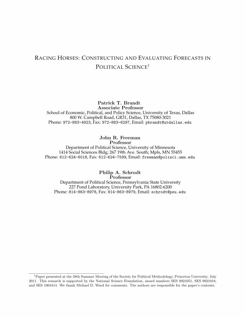
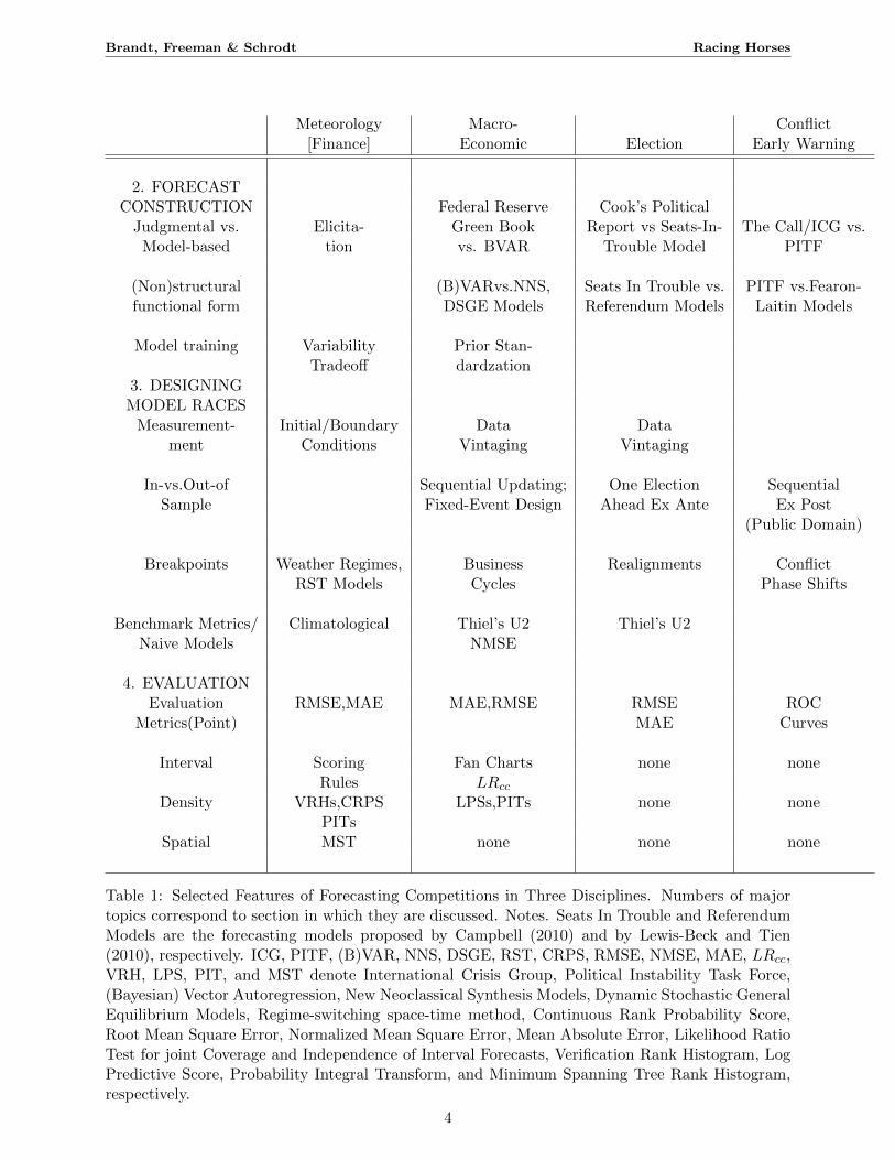
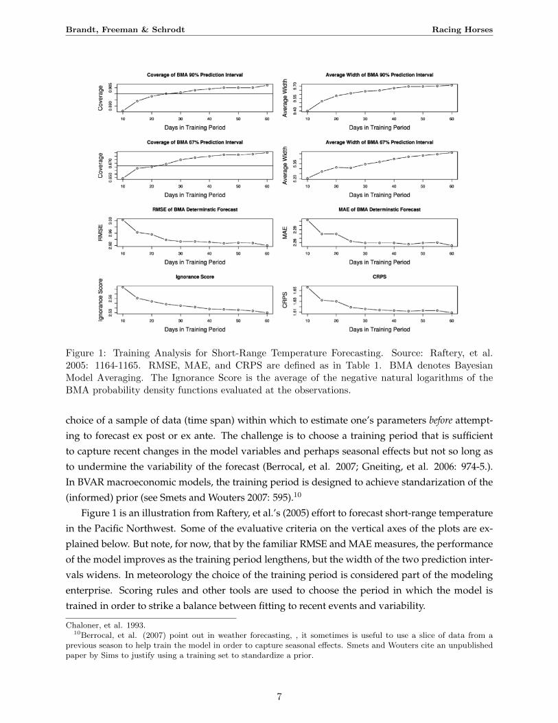
Figure 1: Training Analysis for Short-Range Temperature Forecasting. Source: Raftery, et al.2005: 1164-1165. RMSE, MAE, and CRPS are defined as in Table 1. BMA denotes BayesianModel Averaging. The Ignorance Score is the average of the negative natural logarithms of theBMA probability density functions evaluated at the observations.
choice of a sample of data (time span) within which to estimate one’s parameters before attempt-
ing to forecast ex post or ex ante. The challenge is to choose a training period that is sufficient
to capture recent changes in the model variables and perhaps seasonal effects but not so long as
to undermine the variability of the forecast (Berrocal, et al. 2007; Gneiting, et al. 2006: 974-5.).
In BVAR macroeconomic models, the training period is designed to achieve standarization of the
(informed) prior (see Smets and Wouters 2007: 595).10
Figure 1 is an illustration from Raftery, et al.’s (2005) effort to forecast short-range temperature
in the Pacific Northwest. Some of the evaluative criteria on the vertical axes of the plots are ex-
plained below. But note, for now, that by the familiar RMSE and MAE measures, the performance
of the model improves as the training period lengthens, but the width of the two prediction inter-
vals widens. In meteorology the choice of the training period is considered part of the modeling
enterprise. Scoring rules and other tools are used to choose the period in which the model is
trained in order to strike a balance between fitting to recent events and variability.
Chaloner, et al. 1993.10Berrocal, et al. (2007) point out in weather forecasting, , it sometimes is useful to use a slice of data from a
previous season to help train the model in order to capture seasonal effects. Smets and Wouters cite an unpublishedpaper by Sims to justify using a training set to standardize a prior.
7

Brandt, Freeman & Schrodt Racing Horses
2.3 Constructing Forecasts in International Relations
There is plenty of punditry in international relations. Expert predictions of intra- and interna-
tional conflict are offered regularly by many nongovernmental organizations such as The Call and
The International Crisis Group. Few examples of systematic elicitation exist, but model based fore-
casts are increasingly common, notably the CIA-funded PITF and the Defense Advanced Research
Projects Agency (DARPA) Integrated Conflict Early Warning System (ICEWS; O’Brien 2010). The
PITF (Goldstone, et al, 2010) essentially treat their model as nonstructural; they compare its per-
formance to a more structural models such as that Fearon and Laitin’s model (2003) of civil war
onsets as well as to other nonstructural models such as the Beck et al.’s (2000) neural net model.
In Goldstone, et al. (2010: 200), the PITF uses a 200 country-year training set but provides little
justification for using this data set for training; no set of analyses paralleling those in Figure 1
are reported. ICEWS used a six-year training set (1998-2004) and then evaluated forecasts out-of-
sample for 2005-2006, but no justification was provided for this choice of samples, and the error
bounds were not provided for the forecasts.
Some efforts join judgmental and model based forecasts. Bueno de Mesquita (2010) uses ex-
pert opinion to calibrate his expected utility forecasting model, but he does not report employing
systematic elicitation methods. By all indications he makes no effort to gauge, let alone incorpo-
rate, his experts’ uncertainty about key parameters into his rational choice models (on this point
see Brandt, et al. 2011). BVAR models have been used recently to forecast Israeli-Palestinian rela-
tions by Brandt and Freeman (2006) and by Brandt, Colaresi and Freeman (2008). However, these
investigators make no provision for conflict phase shifts (breakpoints) in spite of the voluminous
literature arguing that conflicts like those in the Levant exhibit regularly exhibit such shifts, as
well as earlier empirical work demonstrating such shifts in cluster-analytical studies (Schrodt and
Gerner 2000).
3 Designing Horse Races
3.1 Measurement
Forecasting is plagued with familiar problems like measurement error and temporal aggrega-
tion. If variables are measured with error, forecasts are likely to be inaccurate. Temporal aggrega-
tion can mask causal relationships and thereby make it difficult to forecast accurately. Practically
speaking, the usefulness of a forecast may diminish if only highly temporally aggregated mea-
sures are available.
Meteorological forecasters also face numerous measurement challenges, along with the fur-
ther complication that their forecasts are three dimensional: they predict weather in space both
horizontally and vertically. To set the initial and boundary conditions as well as the parameters
for their models, weather forecasters construct grids for various geographical coverages and for
8
Brandt, Freeman & Schrodt Racing Horses
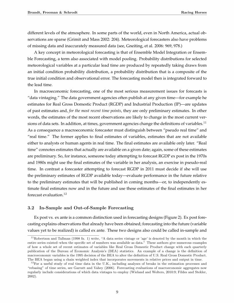
different levels of the atmosphere. In some parts of the world, even in North America, actual ob-
servations are sparse (Grimit and Mass 2002: 204). Meteorological forecasters also have problems
of missing data and inaccurately measured data (see, Gneiting, et al. 2006: 969, 978.)
A key concept in meteorological forecasting is that of Ensemble Model Integration or Ensem-
ble Forecasting, a term also associated with model pooling. Probability distributions for selected
meteorological variables at a particular lead time are produced by repeatedly taking draws from
an initial condition probability distribution, a probability distribution that is a composite of the
true initial condition and observational error. The forecasting model then is integrated forward to
the lead time.
In macroeconomic forecasting, one of the most serious measurement issues for forecasts is
“data vintaging.” The data government agencies often publish at any given time—for example he
estimates for Real Gross Domestic Product (RGDP) and Industrial Production (IP)—are updates
of past estimates and, for the most recent time points, they are only preliminary estimates. In other
words, the estimates of the most recent observations are likely to change in the most current ver-
sions of data sets. In addition, at times, government agencies change the definitions of variables.11
As a consequence a macroeconomic forecaster must distinguish between “pseudo real time” and
“real time.” The former applies to final estimates of variables, estimates that are not available
either to analysts or human agents in real time. The final estimates are available only later. “Real
time” connotes estimates that actually are available on a given date; again, some of these estimates
are preliminary. So, for instance, someone today attempting to forecast RGDP ex post in the 1970s
and 1980s might use the final estimates of the variable in her analysis, an exercise in pseudo-real
time. In contrast a forecaster attempting to forecast RGDP in 2011 must decide if she will use
the preliminary estimates of RGDP available today—evaluate performance in the future relative
to the preliminary estimates that will be published in coming months—or, to independently es-
timate final estimates now and in the future and use these estimates of the final estimates in her
forecast evaluation.12
3.2 In-Sample and Out-of-Sample Forecasting
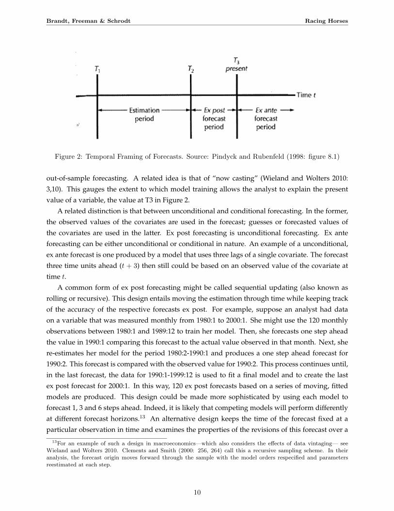
Ex post vs. ex ante is a common distinction used in forecasting designs (Figure 2). Ex post fore-
casting explains observations that already have been obtained; forecasting into the future (variable
values yet to be realized) is called ex ante. These two designs also could be called in-sample and
11Robertson and Tallman (1998 fn. 1) write, “A data series vintage or ’age’ is denoted by the month in which theentire series existed–when the specific set of numbers was available as data.” These authors give numerous examplesof how a whole set of recent estimates of variables like Real Gross Domestic Product change with each quarterlypublication of the Bureau of Economic Analysis’s (BEA) statistics. An example of a change is the definition ofmacroeconomic variables is the 1995 decision of the BEA to alter the definition of U.S. Real Gross Domestic Product.The BEA began using a chain weighted index that incorporates movements in relative prices and output in time.
12For a useful study of real time data in the U.K., including analyses of breaks in the estimation processes and“rebasing” of time series, see Garratt and Vahey (2006). Forecasting evaluations of macroeconomic aggregates nowregularly include considerations of which data vintages to employ (Wieland and Wolters, 2010:9; Fildes and Stekler,2002).
9
Brandt, Freeman & Schrodt Racing Horses
Figure 2: Temporal Framing of Forecasts. Source: Pindyck and Rubenfeld (1998: figure 8.1)
out-of-sample forecasting. A related idea is that of “now casting” (Wieland and Wolters 2010:
3,10). This gauges the extent to which model training allows the analyst to explain the present
value of a variable, the value at T3 in Figure 2.
A related distinction is that between unconditional and conditional forecasting. In the former,
the observed values of the covariates are used in the forecast; guesses or forecasted values of
the covariates are used in the latter. Ex post forecasting is unconditional forecasting. Ex ante
forecasting can be either unconditional or conditional in nature. An example of a unconditional,
ex ante forecast is one produced by a model that uses three lags of a single covariate. The forecast
three time units ahead (t + 3) then still could be based on an observed value of the covariate at
time t.
A common form of ex post forecasting might be called sequential updating (also known as
rolling or recursive). This design entails moving the estimation through time while keeping track
of the accuracy of the respective forecasts ex post. For example, suppose an analyst had data
on a variable that was measured monthly from 1980:1 to 2000:1. She might use the 120 monthly
observations between 1980:1 and 1989:12 to train her model. Then, she forecasts one step ahead
the value in 1990:1 comparing this forecast to the actual value observed in that month. Next, she
re-estimates her model for the period 1980:2-1990:1 and produces a one step ahead forecast for
1990:2. This forecast is compared with the observed value for 1990:2. This process continues until,
in the last forecast, the data for 1990:1-1999:12 is used to fit a final model and to create the last
ex post forecast for 2000:1. In this way, 120 ex post forecasts based on a series of moving, fitted
models are produced. This design could be made more sophisticated by using each model to
forecast 1, 3 and 6 steps ahead. Indeed, it is likely that competing models will perform differently
at different forecast horizons.13 An alternative design keeps the time of the forecast fixed at a
particular observation in time and examines the properties of the revisions of this forecast over a
13For an example of such a design in macroeconomics—which also considers the effects of data vintaging— seeWieland and Wolters 2010. Clements and Smith (2000: 256, 264) call this a recursive sampling scheme. In theiranalysis, the forecast origin moves forward through the sample with the model orders respecified and parametersreestimated at each step.
10
Brandt, Freeman & Schrodt Racing Horses
series of steps; this is called fixed-event forecasting (see Clements and Hendry 1998: 3.2.3).
3.3 More on Breakpoints
Forecasters often assume there is a single causal mechanism—the DGP—that persists over
time. When this mechanism changes, forecasts will suffer from “turning points” and other kinds of
errors (Feldes and Stekler 2002). Moreover, while the addition of causal variables may improve the
performance of a forecasting model when the DGP is constant, the addition of noncausal variables
may improve the forecast when the mechanism is changing (Clements and Hendry 1995: 47ff).
Some researchers try to cope with this problem by introducing contextual variables that control
for such changes (Aron and Meulbauer 2010). Another approach is to employ intercept corrections
(Clements and Hendry 1995). A more challenging approach is to build forecasting models with
explicit nonlinear causal mechanisms to actually predict phase shifts or structural breaks in the
DGP.
From a design standpoint, it is common in macroeconomics for forecasters to evaluate their
models’ abilities to forecast in and across business cycles. For instance, Smets and Wouters (2007)
fit their models during the Great Inflation of 1966:2-1979:2 and during the Great Moderation of
1984:1-2004:4. Wieland and Wolters (2010) fit their forecasting models for U.S. economy for peri-
ods before and after turning points identified by the National Bureau of Economic Research.
3.4 Benchmarks and Naıve Models
Many forecasters include in their designs benchmarks and/or naıve models of various kinds.
A common benchmark is the “no change forecast.” The idea is that useful forecasts, at a mini-
mum, should be able to outperform a forecast of no change in the variable of interest. One of the
most well-known benchmark measures is Thiel’s U (1966: 27-28). Suppose that Pi and Oi are the
predicted and observed values of a variable for some set of data i = 1, . . .,n. Then Thiel’s U or
“inequality coefficient,” is defined as
U2 =
∑ni=1(Pi −Oi)
2∑ni=1O
2i
. (1)
If there is no error in any of the forecasts, U = 0; if the forecasts are for no change in the variables,
U = 1. If the forecasts are actually worse than the forecast of no change, U ≥ 1. Related measures
that use the same benchmark model, essentially the flat forecast function of the random walk
model, are explained below.14 A related idea is that of normalized mean square error, ENMSE .
14Equation (1) is the original definition of U (Thiel 1966); the coefficient is expressed as a second degree polynomial.Despite this formulation, as will be explained in the next subsection, the numerator in the expression on the rightside of the equation is called the root mean square error score. Thiel (1966:28) gives the example of the quotienton the right side of the formula equaling .63. This means that 63% of the root mean square error would have beenobserved had the forecast had been for no change in the variable of interest. For a further discussion of Thiel’s U andits application in macroeconomics see Armstrong and Collopy 1992, Clements and Hendry 1998: 3.2.4, and Fildes
11

Brandt, Freeman & Schrodt Racing Horses
This measure compares the errors from the point predictions of a model to those produced by
using the mean of the observations in the training set for all predictions.15
Univariate AR and VAR models sometimes are treated as benchmarks for forecasting. One
reason for using AR and VAR models as naıve benchmarks is that some analysts consider them
atheoretical. But it also possible view such models as reduced forms of structural models, and
there is a very large theoretical literature suggesting that most organizational behavior is in fact
strongly autocorrelated.16 For example, Aron and Muelbauer (2010) use these models as bench-
marks in their recent effort to forecast U.S. inflation.
A parallel idea in meteorology is the reference forecast, a climatological as opposed to a model-
based forecast. Reference forecasts are used to calculate skill scores for competing models.17 In-
terestingly, meteorological forecasters also sometimes use AR and VAR models as benchmarks
forecasting tools (Gneiting, et al. 2006).
3.5 Designing Horse Races in International Relations
While data vintaging seems not to be a problem for international relations forecasters, mea-
surement error and temporal aggregation are.18 One of the main variables used in the PITF fore-
casting model is based on the POLITY IV measures of democracy, and these measures recently
have been shown to be plagued by measurement error (Treier and Jackman 2008). The forecasting
model used by the PITF also is highly temporally aggregated; its forecasts are for two year hori-
zons. Hence it does not tell policy makers much about the prospects for violence and instability
in the short-term. Some short-term forecasting tools have no time metric such as predictions for
events “some time in the future” (Bueno de Mesquita 2010). Applications of time series models
like BVAR, on the other hand, are much more temporally disaggregated and hence potentially of
more value to policy makers (Brandt and Freeman 2006, Brandt et al. 2011).
International relations forecasters use ex post and ex ante designs, although no forecasters we
are aware of employ an ex ante conditional designs. The PITF (Goldstone, et al. 2010: 200ff)
and Stekler 2002.15Formally we have
ENMSE =
∑t(y
t − yt)2∑t(y
t −meantrain)2(2)
where yt is the observation at time t, yt is the point prediction at time t, and meantrain is the mean of theobservations of yt in the training set. Weigand and Shi (2000) use this metric in conjunction with two approaches todensity forecasting in their analysis of S & P 500 stock returns.
16The idea of using ARIMA models as benchmarks for macroeconomic forecasting models was suggested years agoby Dhrymes, et al. (1972).
17Skill scores are described in more detail below. Gneiting and Raftery (2007: 362) write that ”a reference forecastis typically a climatological forecast, that is, an estimate of the marginal distribution of the predictand. For example,a climatological probabilistic forecast for maximum temperature on Independence Day in Seattle, Washington mightbe a smoothed version of the local historical record of July 4 maximum temperatures.” For another application seeRaftery, et al. 2005, esp. pps. 1157, 1166.
18However, see Lebovic (1995) for an extended discussion of the vintaging issues in at least one form of IR data,published military expenditure estimates by the United States Arms Control and Disarmament Agency.
12
Brandt, Freeman & Schrodt Racing Horses
employed a design that appears to be of the sequential updating type. But, in fact, it is more id-
iosyncratic. To show that an analyst armed with their model in 1994 could do a good job forecast-
ing instability in the period 1995-2004, the PITF takes the model they constructed from a random
subsample of country years for the entire data period 1995-2004, fits an unconditional logit model
to data for the period 1955-1994, and then uses it to sequentially forecast all country-years from
1995-2004. In other words, the PITF assumes that somehow their hypothetical analyst in 1994 was
informed by information from the period they forecast ex post. Also, unlike some parallel work
in macroeconomic forecasting, the PITF does not keep the estimation time span constant in their
sequential forecasting. Rather, the time span of the data used to estimate their forecasting model
increases as each year of data is added to the analyst’s sample. Why this design is preferred to the
more conventional form of sequential updating described above is not explained by the PITF. 19
The idea of break points is at the heart of conflict research. For decades scholars have argued
that conflicts shifts back and forth between different phases. These phase shifts have been inter-
preted as multiple equilibria of games of incomplete information and attributed to the invasion of
dynamic versions of such games by certain strategies (Diehl, 2006), to path dependent sequences
of cooperative and conflictual events (Schrodt and Gerner 2000, Huth and Allee 2002a), to multiple
equilibria in strategies played by audiences and elites in two-level games in (non)democracies (Ri-
oux 1998, Huth and Allee 2000b, Rousseau 2005), and to psychological triggers that produce dif-
ferent types of cooperative and conflictual behavior (Keashly and Fisher 1996, Sense and Vasquez
2008). Unfortunately, we know of no forecasting models that incorporate these and other sources
of phase shifts.20
4 Forecast Evaluation
This is a critical topic that, put simply, has not been studied by most political scientists. Con-
sider the most simple, textbook version of a forecasting model: the linear, two variable (structural)
regression model with constant coefficients (Pindyck and Rubenfeld 1998: Chapter 8). Say this
model is Yt = α+ βXt + εt and that εt ∼ N(0, σ2). The estimate of the model’s error variance is
s2 =1
T − 2
T∑i=1
(Yi − Yi)2. (3)
19This description of the PITF is inferred from is a somewhat cryptic passage on page 200 of the Goldstone etal article (2010). What is difficult to interpret is the ability of an analyst in 1994 to specify a forecasting modelusing some data that he or she could not have observed yet (20 instability onsets and 180 control cases that occurredbetween 1995 and 2004). Second, as regards the hypothetical training set he would have used from 1994 onwards, itis not clear that it is advisable for an analyst to gradually expand the time span of the data set as he sequentiallyforecasts into the future (rather than keeping the span of the data used for estimation constant). No defense of thisdesign feature is offered by the PITF in this passage of their article.
20Recently Park (2010) has proposed break point models to study presidential use of force and certain topics ininternational political economy. But Park’s models only allow for one way state transitions to some terminal state. Hismodels do not allow for state transitions back and forth between states, as we would expect in intra and internationalconflict.
13

Brandt, Freeman & Schrodt Racing Horses
Figure 3: Forecasts From The Simple, Two Variable Regression Model. Source: Pindyck andRubenfield 1998: Section 8.3
For the one step ahead point estimate at T + 1, the estimated forecast error variance is:
s2f = s2[1 +1
T+
(XT+1 − X)2∑Ti=1(Xt − X)2
] (4)
The normalized error is YT+1−Yt+1
sfwhich is t distributed with T − 2 degrees of freedom. The 95%
confidence interval for the forecast at T + 1, YT+1, is:
YT+1 − t.05sf ≤ YT+1 ≤ YT+1 + t.05sf . (5)
This basic forecasting model is depicted in Figure 3. The least squares estimates of the co-
efficients of the model are denoted by α and β. The confidence interval is represented by the
solid lines. This interval shows that, even though the forecast may be presented as a point (fixed
value), YT+1, there is a band of uncertainty associated with it; the forecast errors are assumed to
be drawn from a particular probability distribution. The forecast is a probability density, under
the normality assumption, is centered at Yt+1.21
The problem is that many political scientists only report and evaluate the point forecast, and
even then they do this uncritically, for instance, by the use of measures like root mean square
forecast error that are highly sensitive to outliers. Political scientists do not incorporate into their
21Tay and Wallis (2000: 235) stress that “a density forecast is implicit in standard construction and interpretationof a symmetric prediction interval.”
14

Brandt, Freeman & Schrodt Racing Horses
forecast evaluations either the confidence interval or the forecast density. This hampers our ability
to evaluate the relative performance of our models, especially nonlinear models that are needed
for early warning international conflicts (nonlinear models that allow for conflict phase shifts). As
we explain below, the absence of interval and density forecasting in political science also weakens
the decision theoretic underpinnings of our analyses.
There are essentially three kinds of forecasting and evaluation. In the first, forecasts can be
presented as fixed points; a wide range of evaluation metrics are used to compare these points and
our observations. Forecasts as intervals around the fixed points are the second type; evaluations
are then counts (tests) of the number of times the observations fall into the intervals. In the third
type, forecasts are probability mass functions (densities); evaluations are scores (tests) according to
rules for comparing forecasts with the observed frequencies (distributions) of observations. In the
following subsections, we review each type of forecast evaluation. Then, once again, we critically
evaluate international relations forecasting showing why and how our evaluations should employ
the full suite of evaluative tools.
4.1 Evaluation Metrics for Point Forecasts
More than a dozen metrics for evaluating point forecasts have been studied in the literature.
Armstrong and Collopy (1992) evaluated a collection of metrics for eleven models and for 90 an-
nual and 101 quarterly time series. The six metrics they emphasized were Root Mean Square Error
(RMSE), Percent Better (PB), Mean Absolute Percent Error (MAPE), Median Absolute Percent Er-
ror (MdAPE), Geometric Mean Relative Absolute Error (GMRAE) and Median Relative Absolute
Percent Error (MdRAE). Relative error was defined in terms of a random walk benchmark. The
formulae for these and some related metrics are given in the Appendix.22
Armstrong and Collopy stressed two criteria. The first was reliability. This is the extent to
which a metric produces the same model ranking over a set of horizons and time series. Con-
struct validity was the second metric. It is a measure of how well the metric captures the true
performance of a forecasting model. Armstrong and Collopy conclude that the GMRAE is most
useful for choosing model parameters, the MdRAE is preferred for choosing among parameter-
ized models for a small number of time series, and the MdAPE is most useful for choosing among
parameterized models for a large number of time series. While they note that decision makers find
RMSE easy to interpret—albeit if our experience with generations of students is any indication,
they are probably not interpreting the full impact of squaring the error correctly—they recommend
against the use of RMSE. This metric, which often is also called root mean squared forecast error,
RMSFE, proved highly unreliable in their study (due to its sensitivity to outliers).23
22Recall that a pure random walk has a flat forecast function. The unconditional expectation of the random walk isa constant (y0). The conditional expectation of a random walk is its current value; for a random walk model writtenyt+1 = yt + εt, Etyt+1 = Et[yt + εt] = yt. See, for instance, Enders (2010: 184ff).
23The eleven forecasting tools used by Amstrong and Collopy are a subset of the twenty four tools that wereevaluated in Makridakis, et al. (1982). These include “extrapolation” methods as well as forecasting models (on
15
Brandt, Freeman & Schrodt Racing Horses
In their assessment of the use of the point forecasts in macroeconomics, Clements and Hendry
(1998: Chapter 2) explain as “First Principles” the optimality of conditional expectation, and how
under certain conditions, for a given information set, conditional expectation is unbiased; it pro-
duces minimum mean squared forecast error. They show this for different step-ahead forecasts for
AR(1), ARMA, and VAR(1) models. They also explain why this predictor is optimal for squared
error loss functions (loss functions that put greater emphasis on large vs. small errors and which
associate a equal loss with over and under prediction;ibid. Section 3.2.1). Clements and Hendry
propose the general forecast error second moment matrix and its determinant, denoted by GFESM,
as an (invariant) measure of forecast accuracy. Nonetheless, the use of the RMSFE is still common
in macroeconomics, for example in the recent forecasting efforts by Centre for Economic Policy
Research (Aron and Muelbauer 2010, Wieland and Wolters 2010).
Two additional point forecast criteria should be mentioned. When the variable of interest is bi-
nary in nature, Receiver-Operator Characteristic Curves (ROC curves) sometimes are used. These
curves plot the relative frequency of Type I and Type II errors as a function of the cut points that
determine each value of the binary variable. The intention of the ROC curve is to provide a cal-
ibration of the test based on the relative cost to the decision maker from each kind of error. In
recent years, one is also seeing the ROCs area under curve (AUC) measures used to assess overall
predictive accuracy. As Sing, et al. (2009:3) note, “[AUC] is equal to the value of the Wilcoxon-
Mann-Whitney test statistic and also the probability that the classifier will score a randomly drawn
positive sample higher than a randomly drawn negative sample.” An AUC of 0.5 indicates that
the model is only performing as well as chance. Ulfelder [2011] observes that in political forecast-
ing,“An AUC of 0.5 is what you’d expect to get from coin-flipping. A score in the 0.70s is good; a
score in the 0.80s is very good; and a score in the 0.90s is excellent.”24
The other criteria is termed “rationality testing.” This is the practice of fitting simple regression
models for observed and forecasted values of variables and then testing the joint condition of a
zero intercept and a value of unity for the coefficient on the forecasted values. That is, one fits the
regression:
yt+k = a+ byft (k) + µt (6)
where yt+k is the observed value at time t at forecast horizon k, yft (k) is the forecasted value at time
t+k, µt is a iid normally distributed error term with zero mean. It is rational to use the forecasted
values if a=0 and b=1 and the error term in (6) is not serially correlated.25
this distinction see Chatfield 1993: 122-123). Other criteria considered by Armstrong and Collopy include Under-standability, Sensitivity (how performance changes with changes in model parameters) and Relationship to DecisionMaking. They are careful to note in their conclusion that their results may differ for evaluating a model’s performanceon a single time series and also that their design did not include ”turning points.”
24http://dartthrowingchimp.wordpress.com/2011/06/09/forecasting-popular-uprisings-in-2011
-how-are-we-doing/. Accessed 10-Jun-2011.25See Fildes and Stekler (2002: esp. 440). They describe several tests for rationality and also discuss the necessary
and sufficient conditions for a forecast to be rational. See also Clements and Hendry (1998: Section 3.2.2.)
16

Brandt, Freeman & Schrodt Racing Horses
Figure 4: Fan Chart for Inflation Forecast of the Bank of England. Source: Gneiting 2008: 320
4.2 Interval Forecasts
Interval forecasts are used when the full predictive distribution for a variable is not available.
They are a special case of a more general type of evaluation called quantile prediction (Gneiting
and Raftery 2007: 370). Interval forecasts recognize the uncertainty attached to point forecasts and
provide decision makers with an idea of the range of values a random variable might take at some
future date. As such they are useful for contingency planning and other purposes.
The key concept is the “prediction interval” or PI.26 PIs differ from conventional confidence
intervals insofar as PIs are an estimate of the range of unknown future values of a random variableat the time a forecast is made. Confidence intervals, in contrast, represent the range of what
usually are assumed to be fixed but unknown parameters. PIs now are regularly published for
the macroeconomic forecasts of economic institutes and central banks. An example is the Bank of
England’s inflation forecasts (Figure 4).27
For example, assume that we want to make a forecast of a random variable, Xt, k steps ahead,
Xn+k, and that we have realizations of Xt for times t = 1, . . . , n. Denote these observations by
x1, . . . , xn. Denote our point forecast at n + k by xn(k). In order to construct a 100(1 − α)%-ile
26The following paragraph is a summary of Chatfield (1993, especially pps. 121-124). See also, Chatfield (2001)and Taylor (1999).
27Chatfield (2001) repeats the list of reasons from his (1993) article on why PIs often are not used. But Clementsand Hendry (1998: Chapter 1, fn. 6) say that, like the Bank of England, the U.K. Institute for Economic and SocialResearch also publishes PIs for its forecast. Clements and Hendry note that the Bank of England’s chart is knownfor its “rivers of blood.”
Much work has been devoted to understanding how PIs differ for stationary or nonstationary processes. Forstationary processes, as the forecast horizon becomes longer and longer, var[en(k)] tends to the variance of DGP. Sothe PI will have finite width as k increases (Chatfield 1993: 133). In contrast, for nonstationary DGPs, there is noupper bound to the width of the PI. Clements and Hendry (1998: chapters 6, 11) investigate interval forecasting forthis case. A forecast based on cointegrated series will have PIs with finite limiting PMSE. See Lutkepohl (2006).
17

Brandt, Freeman & Schrodt Racing Horses
PI for Xn+k, we usually use the expression xn(k) ± zα2
√var[en(k)] where en(k) is the conditional
forecast error corresponding to our point prediction and zα2
is the respective percentile point of the
standard normal distribution.28 This equation assumes that the forecast is unbiased or, E[en(k)] =
0 and that the prediction mean squared error (PMSE) E[en(k)2], is equal to var[en(k)]. Once more,
the forecast errors are assumed to normally distributed.
Chatfield (1993) analyzes the effects of parameter uncertainty on the estimation of the PIs. He
stresses the challenges of evaluating the var[en(k)], especially when, as is often the case, there
is no analytic expression for the true model PMSE.29 His review includes a critical evaluation of
approximations, empirical, simulation, and resampling methods for estimating var[en(k)]. Chat-
field recommends against using certain approximations. The problem of PIs typically being too
narrow looms large in Chatfield’s discussion. He traces this problem to model uncertainty and
other issues and recommends using 90% (or perhaps 80%) PIs to avoid tail problems (1993: 489).
Christoffersen (1998) develops likelihood ratio tests to evaluate the unconditional coverage and
independence of a series of out-of-sample interval forecasts.30
While interval forecasts were not widely used in the 1980s and early 1990s, they have become
more common in finance and economics. Christofferson’s (1998) work is expressly motivated by
the challenges of risk analysis in general and of modeling the volatility of financial time series in
particular. ARCH and similar models suggest that unconditional forecasting models will produce
intervals that are too wide in times of tranquility and too narrow in times of turbulence in financial
markets. To address this problem, Christoffersen shows how his tests can be applied to evaluate
the PIs produced by dynamic risk models. In this context, he shows, contrary to the conventional
wisdom of the 1990s, that PIs can be too wide as well as too narrow and that a single forecasting
model can produce PIs suffering from both problems during the same (ex post) forecasts.
28Formally, en(k) = Xn+k − xn(k). So en(k) is a random variable.29For some models, an expression for var[en(k)] can be derived. An example is the simple AR(1) without a constant.
The expression in this case is
E[en(k)2] =σ2ε (1− α2k)
(1− α2)(7)
where σ2ε is the variance of the error term in the AR(1) model, α is the AR(1) coefficient, and k is the forecast
horizon. For further derivations of true PMSE for selected models see Chatfield 1993: Section 4.2, Clements andHendry Chapter 4, and, for selected, multivariate and simultaneous equation models, Lutkepohl 2006.
30Briefly, for an observed sample path of a time series yt, (yt)Tt=1, a series of interval forecasts is denoted by
[(Lt|t−1(p), Ut|t−1(p))]Tt=1 where Lt|t−1(p) and Ut|t−1(p) are the lower and upper bounds of the ex ante intervalforecast for time t made at time t−1 with coverage probability p. Christoffersen defines an indicator variable, It thatis 1 when the realization is in the interval and 0 otherwise. He then defines a sequence of interval forecasts as efficientwith respect to information set Ψt if E[It|Ψt−1] = p for all t. He proves that testing E[It|Ψt−1] = E[It|It−1, . . . , It] = pfor all t, is equivalent to testing that the sequence It is iid Bernoulli with parameter p. He defines a sequence ofinterval forecasts as having correct conditional coverage in this sense. Christoffersen goes on to derives three likelihoodratio tests for interval forecasts: for unconditional coverage (LRuc), for independence (LRind), and for coverage andindependence jointly (LRcc). In order to address the problem of model uncertainty, Christoffersen designed his teststo be model (method) and distribution free.
18
Brandt, Freeman & Schrodt Racing Horses
4.3 Evaluating Probabilistic Forecasts: Scoring Rules and the Concepts Cali-
bration and Sharpness
The case for probabilistic forecasting forecasting was made in a classic paper by Dawid (1984).31.
The idea is to elicit from an assessor (judgmental forecasting) or produce from a model a probabil-
ity density (mass function) over future quantities or events. For example, for continuous random
variables, a density forecast is “a complete description of the uncertainty associated with a pre-
diction, and stands in contrast to a point forecast, which by itself, contains no description of the
associated uncertainty” (Tay and Wallis 2000: 235). Decision theory shows that while in general it
is impossible to rank two incorrect forecast densities for two forecast users, if the forecast density
corresponding to the true data generating process can be found, all forecast users will prefer that
density regardless of the loss functions they employ.32 In addition, density forecasts help analysts
discriminate between linear and nonlinear models (Clements and Smith 2000) and cope with low
signal to noise ratios in time series data (Weigand and Shi 2000).33
The evaluation criteria for probabilistic forecasts include calibration and sharpness. Calibra-
tion is the statistical consistency between the distributional forecasts and observations. Sharpness
deals with the “concentration of [the] predictive distribution and is a property only of the fore-
casts” (Gneiting and Raftery 2007: 359). The goal of probabilistic forecasting is to achieve a high
degree of sharpness subject to calibration.34
Among the tools used in these evaluations are scoring rules. These assign a number that rep-
resents the degree of association between the predictive distribution and observed events. Those
scores are used to rank the success of forecasters and of models and are an integral part of what
meteorologists call “forecast verification.” A scoring rule is “proper” if it gives an assessor an in-
centive to reveal her true probability mass function (density) rather than to “hedge (supply equal
probabilities for each event, for example). Model fitting can be interpreted as the application of
31Precursors are Rosenblatt, (1952) and Pearson (1933)32Tay and Wallis (2000: 236) explain that different loss functions may lead to different optimal point forecasts if
the true density is asymmetric.Briefly, Diebold, et al. (1998) explain the advantages of finding the forecast density corresponding to the true data
generating process. They compare the action choice for what is believed to be the correct density, p(y), for a variableyt with realizations ytmt=1 with the action choice for what is the true data generating process, f(y). They showthat, if two decision makers have different loss functions, and, if neither of two forecast densities j and k, pj(y) andpk(y), are correct, it not possible to rank these densities. One decision maker might prefer to use pj(y) while theother decision maker might prefer to use density pk(y). They give an example in which the true density is Nor(0, 1),the two incorrect densities are Nor(0, 2) and Nor(1, 1), and one decision maker bases her choice on the forecast meanwhile the other bases his decision on the error in the forecast of the uncentered second moment. But, again, if theycan find the true forecast density, in their illustration, Nor(0, 1), these and all other decision makers will prefer touse it. See Diebold, et al. 1998: 865-866 for a fuller, formal development of this result.
33For instance, Clements and Smith (2000) explain why point metrics usually don’t show nonlinear models to besuperior at forecasting in comparison to linear models. They then show how density forecast evaluation methodscan be used to compare the performance of linear and nonlinear models (AR and SETAR) and linear and nonlinearmultivariate models (VAR and Nonlinear VAR).
34See also Raftery, et al. 2005. Hamill (2001: 551-552) equates the concepts of calibration and “reliability”.Gneiting, et al. 2007 develop three concepts of calibration: probabilistic, exceedance and marginal. We focus on thefirst of these here.
19

Brandt, Freeman & Schrodt Racing Horses
Rule Form Range
Quadratic Q(r, d) 1−∑
i(ri − di)2 [-1,1]
Brier PS(r, d) 1−Q(r, d) [0,2]
Spherical S(r, d)∑i ridi
(∑i r
2i )
12
[0,1]
Logarithmic L(r, d) ln(∑
i diri) (−∞, 0]
Table 2: Four Well Known (Proper) Scoring Rules for Discrete Random Variable Forecasts
optimum score estimators, a special case of which is maximum likelihood.35
There are several well known scoring rules for discrete random variables.36 Consider a vari-
able that produces n discrete and mutually exclusive events, E1, . . . , En. Say that an assessor sup-
plies at time t a judgmental, probabilistic forecast about the values the variable will assume at
time t + 1. This probabilistic forecast is in the form of a row vector r = (r1, . . . , rn) where ri is
her elicited probability that event i will occur. Let her true assessment be represented by the row
vector p = (p1, . . . , pn). Finally let the row vector d = (d1, . . . , dn) denote the actual observation at
t + 1 so that, if event i is realized, di = 1 and dj = 0 for j 6= i. Then an assessor (judgmental fore-
caster) is considered perfect in the normative sense if her probability vector, r, is “coherent”—it
satisfies the laws of probability—and her vector corresponds completely to her true beliefs (r = p).
The idea of a proper scoring rule is one that makes it rationale for this last condition to be satisfied
(r = p), or a rule for which reporting p maximizes the assessor’s expected score (utility).
Some examples of such rules are described in Table 2; all of these are proper rules. For instance,
the logarithmic scoring rule was suggested by Good (1952). It is sometimes called an “ignorance
score.” It also is a “local rule” insofar as its value depends only on the probability assigned to
outcome that actually is observed, not on the probabilities assigned to outcomes that are not ob-
served.37
As an illustration, consider the event that precipitated the Gulf War: Iraq’s invasion of Kuwait.
Suppose that there were only three possibilities (n = 3): ground invasion, air attack, and no inva-
sion. Suppose that through an elicitation tool, forecasters A and B supplied the vectors (.35, .60,
35Gneiting and Raftery (2007) provide a theory of proper scoring rules on general probability spaces. They explainthe relationships between these rules and information measures and entropy functions. As regards estimation, theyexplain how proper scoring rules suggest useful loss functions from which optimum scoring estimators can be derived.Finally, they explain the link between proper scoring rules and Bayesian decision analysis.
36The following passage is a condensation of Winkler and Murphy (1968: 753-5). A more general treatment ofscoring rules for forecasting models of discrete variables is Gneiting and Raftery 2007: Section 3.
37For example, to show that the quadratic scoring rule, Q(r, d) in Table 2, is proper, Winkler and Murphy (1968:754) note that the assessors expected score for this rule is:
E(Q) =∑j
pjQj(r, d) =∑j
p2j −∑j
(rj − pj)2, (8)
which is maximized when r = p. They also show that the spherical and logarithmic rules also are proper.
20

Brandt, Freeman & Schrodt Racing Horses
Forecaster Q(r, d) Brier PS S(r, d) L(r, d)
A .215 .785 .503 -1.050B .265 .735 .518 -1.204
Table 3: Illustrative Scores for Two Hypothetical Forecasters for Iraq’s Behavior in 1991. ForecasterA: (.35, .60,. 05); Forecaster B: (.30, .35, .35).
.05) and (.30, .35,and .35), respectively. Iraq launched a ground invasion of Kuwait, so event E1
was realized. As Table 3 shows, forecaster B would have received a higher score according to the
quadratic and spherical scoring rules whereas forecaster A would have received a higher score
according to the logarithmic score. The Brier PS score, because its interpretation is the reverse of
the quadratic score, also would rank forecaster B more proficient than forecaster A. These rank-
ings reflect the fact that the logarithmic scoring rule emphasizes the assessed probability only of
the event that actually occurred whereas the other rules incorporates all the assessed probabilities
relative to this realization.38
For evaluating forecasts of ordered categories of a discrete random variable, the Ranked Prob-
ability Score (RPS) often is used. The RPS includes an evaluation of the “distance” between the
realization and the relative probabilities assigned by a forecaster to the different (ordered) cate-
gories of events. Assume that there are K such categories and that the assessor’s forecast is the
row vector (p1, . . . , pK). Then the scoring rule for when each observation j actually occurs is:
Sj =3
2− 1
2(k − 1)
K−1∑i=1
[(i∑
n=1
pn)2 + (K∑
n=i+1
pn)2]− 1
K − 1
K∑i=1
|i− j|pi. (9)
Sj ranges from 0 for the worse possible forecast to 1 for the best forecast. It also is a proper scoring
rule.39
For example, say that a particular intra state conflict moves back and forth between four con-
flict phases.40 Call the count of conflictual events at time t, Ct. And assume that the phases are
defined by an ordered set of categories of such counts. To be more specific, for phase 1: Ct = 0-10;
phase 2: Ct = 11-20; phase 3: Ct= 20-30; and phase 4: Ct > 40. When asked what phase the con-
flict will be in in (t+1) analyst A provides the forecast (.1, .3, .5, .1) while analyst B provides the
forecast (.5, .3, .1, .1). The scores according to this rule for the two analysts are reported in Table
4. Note that, if the highest phase of the conflict is realized, phase 4, analyst A scores .67 while his
counterpart scores .43. This is because analyst A assigns more overall probability to phases 3 and
38When the quadratic score implies the best performance, Q(r, d) = 1, PS = 1 − 1 = 0. Conversely, when theQ(r, d) = −1, Brier PS = 1 − −1 = 2. For an exposition of the Brier score and its relation to Finetti’s work instatistics, see Seidenfeld 1985: 287.
39The classic paper on the RPS is Epstein (1969). Epstein derives the rule from in a decision theoretic frameworkthat represents costs and losses associated with preparing for and experiencing meteorological events. Seemingly inresponse to practice of hedging, Epstein also derives a version of the scoring rule for the case in which assessors assignequal probability to all K categories.
40The following example is based on the weather illustration in the original Epstein article (1969).
21

Brandt, Freeman & Schrodt Racing Horses
Observed Analyst A Analyst Bcategory (.1,.3,.5,.1) (.5,.3,.1,.1)
1 .61 .902 .87 .903 .94 .704 .67 .43
Table 4: Rank Probability Scores for Conflict Phase Forecasts by Two Hypothetical Analysts
4 than analyst B. Conversely, if phase 1 or 2 is realized, analyst B would perform better since he
assigns more probability to these phases than analyst A.
Suppose the analyst or model produces a predictive density function (PDF ) for future val-
ues of a variable. In the case of human subjects this might be accomplished by means of certain
kinds of elicitation.41 Predictive densities might be obtained from models either by making dis-
tributional assumptions about estimation uncertainty or, as is increasingly common, by means of
computation (Brandt and Freeman 2006, 2009). In this case evaluative tools differ according to
whether they are based on binary scoring rules which are defined on the probability space (unit
interval) or on payoff functions that are defined on the space of values of the variable of interest
(real line).42
There are limiting versions for the three scoring rules of the first type we described above for
discrete variables.43 Assume x is the observed value of the variable we are trying to forecast and
that r(x) is a probability density supplied by the analyst or model. Then the continuous analogues
of the earlier scoring rules are, respectively:
Quadratic: S(r(x)) = 2r(x)−∫ ∞−∞
r2(x)dx (10)
Logarithmic: S(r(x)) = log[r(x)] (11)
Spherical: S(r(x)) =r(x)
[∫∞−∞ r
2(x)dx]12
. (12)
These rules also are strictly proper and each has distinct properties. For example, the logrithmic
rule penalizes low probability events; it is highly sensitive to extreme values. As we explain in
Appendix 2, these rules can be generalized into a collection of formulae for predictive densities all
of which are based on a simple binary form of scoring.
One of the most widely used scoring rules is the Continuous Rank Probability Score (CRPS).
The CRPS is defined as follows (Hersbach 2000: 560-1): let the forecast variable of interest again
be denoted by x, the observed value of the variable by xa, and the analyst’s (or model’s) PDF by
41A review of these elicitation methods and an application to terrorist network analysis is Freeman and Gill (2010).42On this distinction see Matheson and Winkler (1976: 1092, 1095). These authors also use the distinction
probability-oriented and value-oriented in this context. See Figures 9 and 10 in Appendix 2.43These examples come from Matheson and Winkler (1976: 1089)
22
Brandt, Freeman & Schrodt Racing Horses
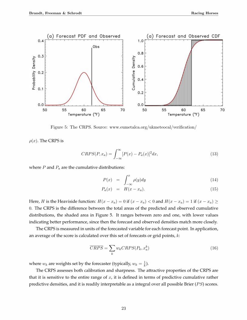
Figure 5: The CRPS. Source: www.eumetalca.org/ukmeteocal/verification/
ρ(x). The CRPS is
CRPS(P, xa) =
∫ ∞−∞
[P (x)− Pa(x)]2dx, (13)
where P and Pa are the cumulative distributions:
P (x) =
∫ x
−∞ρ(y)dy (14)
Pa(x) = H(x− xa). (15)
Here, H is the Heaviside function: H(x− xa) = 0 if (x− xa) < 0 and H(x− xa) = 1 if (x− xa) ≥0. The CRPS is the difference between the total areas of the predicted and observed cumulative
distributions, the shaded area in Figure 5. It ranges between zero and one, with lower values
indicating better performance, since then the forecast and observed densities match more closely.
The CRPS is measured in units of the forecasted variable for each forecast point. In application,
an average of the score is calculated over this set of forecasts or grid points, k:
CRPS =∑k
wkCRPS(Pk, xka) (16)
where wk are weights set by the forecaster (typically, wk = 1k ).
The CRPS assesses both calibration and sharpness. The attractive properties of the CRPS are
that it is sensitive to the entire range of x, it is defined in terms of predictive cumulative rather
predictive densities, and it is readily interpretable as a integral over all possible Brier (PS) scores.
23
Brandt, Freeman & Schrodt Racing Horses
Approaches to computing the CRPS are discussed in Gneiting and Raftery (2007: Section 4.2).44
Verification rank histograms (VRHs) or Talagrand diagrams are one of the main tools used to
assess calibration. Gneiting, et al. (2007: 252) call the VRH the “cornerstone” of forecast evalua-
tion. Hamill (2001: 551) explains the idea behind the the VRH for forecasting ensembles:
. . . if ensemble relative frequency suggests P per cent probability of occurrence
[of an event], the event truly ought to to have P probability of occurring. For this
probability to be reliable [calibrated], the set of ensemble member forecast values at
a given point and the true state (the verification) ought to be able to be considered
random samples from the same probability distribution. This reliability [calibration]
then implies in turn that if a n-member ensemble and the verification are pooled into
a vector and sorted from lowest to highest, then the verification is equally likely to
occur in each of the n + 1 possible ranks. If the rank of the verification is tallied and
the process repeated over many independent sample points, a uniform histogram over
the possible ranks should result.
For each forecast the rank of the observed value is tallied relative to the sorted (ranked) ensem-
ble forecasts. The population rank j then is the fraction of times that the observed value (“truth”),
when compared to the ranked ensemble values, is between ensemble member j − 1 and j. For-
mally, rj = P (xj−1 ≤ V < xj) where V is the observed value, x is a sorted ensemble forecast of
the indicated rank and P is the probability. If the ensemble distribution is calibrated, these ranks
will produce a uniform histogram.
A related concept is the probability integral transform (PIT). This is defined in terms of realiza-
tions of time series and their one step ahead forecasts. Let ytmt=1 be a series of realizations from
the series of conditional densities f(yt|Ωt−1)mt=1 where Ωt−1 is the information set. If a series of
one-step ahead density forecasts, pt−1(yt)mt=1 coincides with f(yt|Ωt−1)mt=1 the series of PITs of
ytmt=1 with respect to pt−1(yt)mt=1 is i.i.d. U(0, 1) or,
ztmt=1 =
∫ yt
−∞pt−1(u)du
m
t=1
∼ U(0, 1). (17)
The CRPS is defined, in part, in terms of the PIT—via the forecast density. For a collection of
forecasts and series of observed values of a variable, PIT values can be calculated for a set of
forecasts and then these values arranged in a VRH.45
The VRH is used in the two ways: first it is expressed either in terms of familiar relative
44The properties of the CRPS and how it can be decomposition into a reliability, uncertainty, and resolution partare discussed in Hersbach (2000). He explains the connection between the CRPS and the Brier (PS) score and how,for a collection of deterministic forecasts, the CRPS is equivalent to MAE. Gneiting and Raftery (2007) develop thedecision theory for this and the other scores in probability spaces. They also note that atmospheric scientists use theCRPS “negative orientation:” CRPS ∗ (F, x) = −CRPS(F, x). Later in their article the authors explain how theCRPS can be built up from predictive quantiles.
45The definition of the PIT in this paragraph is from Diebold, et al. (1999, 1998). An explanation of how the PITis at the heart of Dawid’s prequential principle is Gneiting, et al. (2007: 244).
24

Brandt, Freeman & Schrodt Racing Horses
Figure 6: Verification Rank Histogram. Source: Gneiting, et al. 2005
frequencies or its continuous analogue, a histogram density with Figure 6 illustrating the first
kind of VRH; see the Appendix for an explanation of the second. Visually, a U-shaped VRH
indicates that the forecasting model is underdispered (too little variability, prediction intervals
are too wide) while a hump-shaped VRH indicates the forecasting model is overdispersed (too
much variability, prediction intervals are too narrow).46 Sometimes a cdf plot is used instead of
the VRH. If the VRH is uniform, its cdf ought to be approximately a 45 degree line (see Clements
and Hendry 2000: 249ff). The χ2 test can be used to assess uniformity; other tests are available for
this purpose such as the Kolmogorov-Smirnov test (Diebold, et al. 1998; Tay and Wallis 2000). For
time series data, it is important to establish, before testing for uniformity, that PITs are i.i.d. using
a correlogram (Diebold, et al. (1998, 1999); Clements and Hendry (2000); Gneiting, et al. (2007:
Section 4.1.)). Hamill (2001) shows that the VRH can be flat despite the fact that the forecasts
suffer from conditional bias. Sampling from the tails of distributions, from different regimes, and
across space without accounting for covariance at grid points all can produce mistaken inferences
from the shape of the VRH. Hamill recommends forming the VRH from samples separated in both
space and time. Diebold, et al. (1998), Diebold, et al. (1999) and Clements and Smith (2000) show
how the PIT and VRHs can be applied in multi-step and multivariate forecasts.47
On the basis of Hamill’s critique of the VRH and an examination of spread-error plots for some
sample data, Gneiting, et al. (2005) and Gneiting, et al. (2007) recommend that an assessment of
46Hamill (2001) provides some simple examples to illustrate how the VRH can reveal over and underdispersion. Heform VRHs by taking draws from truth in the form of a N(0,1) distribution and from biased (incorrect) ensemblesin the form of a collection of normal distributions N(µ, σ) for which µ 6= 0 and(or) σ 6= 1. See also Gneiting, et al.(2007: Section 1).
47The extension of the PIT in multivariate analysis involves decomposing each period’s forecast into its conditionals.See Diebold, et al. (1999: 881) and Clements and Smith (2000:862-3)
25
Brandt, Freeman & Schrodt Racing Horses
sharpness be included in the evaluation of probabilistic forecasts. Recall sharpness has to do with
the concentration of the predictive distribution. Gneiting, et al. (2007) summarize the prediction
intervals with box plots to gauge sharpness of competing meteorological models.
Probabilistic forecasting became prevalent in the late 1990s.48 It is now at the heart of forecast
verification in meteorology. Meteorologists use a suite of the tools described above to evaluate
such forecasts. For instance, Gneiting, et al. (2006) use the CRPS, PIT and RMSE to evaluate the
RST model. Gneiting, et al. (2007) use a combination of calibration tests (PIT) and box plots along
with MAEs, log scores, and CRPS to rank three algorithms for forecasting windspeed. 49 Proba-
bilistic forecasting is employed in finance to study high frequency exchange rate series (Diebold,
et al. 1998) and stock returns (Weigand and Shi 2000), and to evaluate portfolios (Tay and Wallis
2000). The PIT, logarithmic scoring and MSE are used in these studies. Clements and Smith (2000)
use the PIT and VRH as well as some related statistical tests to study a two variable model of
the U.S. macroeconmoy. Some more recent work in macroeconomics uses the log predictive score
(Geweke and Amisano 2009).
4.4 Evaluating Forecasts in International Relations
International relations forecasters expressly run horse races. The PITF goes to great lengths to
compare the performance of its model with those of its competitors (Goldstone, et al. 2010). The
problems with the forecast evaluations of the PITF are a) they only use point evaluation to gauge
the accuracy of competing models and b) they make almost no provision for estimation uncer-
tainty. Accuracy assessments are based on percent correctly predicted under strong assumptions
about cut-points for (un)conditional logit models on the one hand, and comparisons of point based
decile rankings of country probabilities of instability. No other metrics are employed. Equally im-
portant, with the exception of the occasional calculation of confidence intervals for odds ratios
(ibid. Table 1), the PITF never incorporates estimation uncertainty in its analysis; no error bands
are reported either for its percent correctly predicted or its rank comparisons. Claims about the
victories of its models over those based on the work of Fearon and Latin, neural network set-ups,
and other competitors therefore are difficult to evaluate. Earlier critiques of the PITF (King and
Zeng 2001) explain how decision theory can be used to determine cut points, how scoring rules
like ROC curves can be employed in forecast evaluation, and how confidence intervals can be con-
structed for relative risk and first differences. However, these critiques do not do go far enough in
incorporating estimation and other kinds of uncertainty. For example, they do not provide error
48Fildes and Stekler’s (2002) claim that probabilistic forecasting has not caught on in the natural and social sciencesis simply inaccurate. See, for instance, the piece by Gneiting and Rafterty (2005) in Science, and the Introductionto the special issue of the Journal of Forecasting by Timmerman (2000). Diebold, et al. (1998) explain how theuse of probabilistic forecasting increased due to the interest in assessing financial portfolios and improvements inrecalibration methods, more specifically, because, in financial management, the tails and other features of the forecastdistribution are of special interest (VaR).See also the introduction to Geweke and Amisano (2009).
49The information about forecast verification at the University of Washington research center can be found athttp://isis.apl.washington.edu/bma/index.jsp. See also http://probcast.washington. edu
26
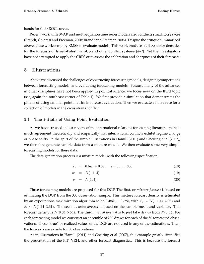
Brandt, Freeman & Schrodt Racing Horses
bands for their ROC curves.
Recent work with BVAR and multi-equation time series models also conducts small horse races
(Brandt, Colaresi and Freeman, 2008; Brandt and Freeman 2006). Despite the critique summarized
above, these works employ RMSE to evaluate models. This work produces full posterior densities
for the forecasts of Israeli-Palestinian-US and other conflict systems (ibid). Yet the investigators
have not attempted to apply the CRPS or to assess the calibration and sharpness of their forecasts.
5 Illustrations
Above we discussed the challenges of constructing forecasting models, designing competitions
between forecasting models, and evaluating forecasting models. Because many of the advances
in other disciplines have not been applied in political science, we focus now on the third topic
(see, again the southeast corner of Table 1). We first provide a simulation that demonstrates the
pitfalls of using familiar point metrics in forecast evaluation. Then we evaluate a horse race for a
collection of models in the cross straits conflict.
5.1 The Pitfalls of Using Point Evaluation
As we have stressed in our review of the international relations forecasting literature, there is
much agreement theoretically and empirically that international conflicts exhibit regime change
or phase shifts. In the spirt of the simple illustrations in Hamill (2001) and Gneiting et al (2007),
we therefore generate sample data from a mixture model. We then evaluate some very simple
forecasting models for these data.
The data generation process is a mixture model with the following specification:
xi = 0.5wi + 0.5vi, i = 1, . . . , 300 (18)
wi = N(−1, 4) (19)
vi = N(1, 4). (20)
Three forecasting models are proposed for this DGP. The first, or mixture forecast is based on
estimating the DGP from the 300 observation sample. This mixture forecast density is estimated
by an expectations-maximization algorithm to be 0.48wi + 0.52vi with wi ∼ N(−1.14, 4.98) and
vi ∼ N(1.11, 3.61). The second, naıve forecast is based on the sample mean and variance. This
forecast density is N(0.04, 5.54). The third, normal forecast is to just take draws from N(0, 1). For
each forecasting model we construct an ensemble of 200 draws for each of the 50 forecasted obser-
vations. These “true” or realized values of the DGP are not used in any of the estimations. Thus,
the forecasts are ex ante for 50 observations.
As in illustrations in Hamill (2011) and Gneiting et al (2007), this example greatly simplifies
the presentation of the PIT, VRH, and other forecast diagnostics. This is because the forecast
27

Brandt, Freeman & Schrodt Racing Horses
Mixture Naıve Normal
RMSE 2.79 3.33 2.58MAE 2.25 2.68 2.10
CRPS 1.44 1.37 1.53Logarithmic(IGN) 2.65 2.29 3.82
Table 5: Forecasting model assessment measures.
performance measures are not confounded by the presence of serial correlation which can greatly
affect perceived forecast performance. The three models also forecast (nearly) the same mode, so
we can focus on the distributional fit of the true model versus its inferior competitors.
Table 5 presents the average RMSE, MAE, CPRS, and ignorance (IGN) measure for the forecast
ensembles for each model.50 The best forecasting performance on each metric is highlighted in
bold.
The key conclusion based on these forecast performance metrics is that the “true model” is never thewinning horse. The forecasting performance of the true model is nearly the same as the “winner”,
but the mixture model is never in fact the winner. This illustrates the earlier point that using a
single metric like the familiar RMSE or MAE tells us little about forecasting performance.
More useful is a comparison based on the PIT or the VRH. Figure 7 presents these plots. Recall
that better fitting models have uniform PIT and VRH histograms. Models that have underdis-
persed forecasts have U-shaped plots; those, that are humped indicate overdispersion. The PIT
plots show that the normal forecast is underdispersed:the forecast ensemble variability is lower
than that observed in the data. Both the mixture and naıve forecast have flatter PIT plots. We
see here why the average CRPS is slightly better for the naıve model: it covers the tails of the
distribution slightly better than the mixture model, but not by much.
The VRH gives the number of times a forecast in the ensemble is greater than the observed
value. This is why the histogram’s x-axis runs from 0 to 200, since forecast ensemble could theo-
retically never or always be above the true value.51 Here, the VRH of the normal forecast deviates
from uniformity, while the VRH’s of the mixture and naıve forecasts are closer to uniformity. For-
mally, one can test for the distributional equivalence we are analyzing here using a Komolgorov-
Smirnov test for whether the VRH is uniform. Employing this test, the p-values are 0.13 for the
mixture forecast, 0.95 for the naıve forecast, and 0.02 for the normal forecast. So we have strong
evidence against the forecast distribution being N(0, 1), but cannot make a clear choice between
the mixture and naıve forecasts, since both have uniform VRHs.52
50The ignorance metric is the negative log density of the forecast errors, evaluated at the observed data. Smallervalues thus indicate more agreement between the forecast and the observed data.
51So for example, consider the VRH in the southeast corner of Figure 7, the VRH for the N(0,1) forecast. The firstbar in the VRH has height 14. This means that 14 times in the forecasting exercise (out of 50 total) none of the 200forecasts in a given ensemble were larger than the true value taken from the DGP.
52We can apply the Komolgorov-Smirnov test to assess the uniformity of the PITs as well. For each forecast modelthe PIT deviates from uniformity based on this test.
28

Brandt, Freeman & Schrodt Racing Horses
PIT from mixture forecast
Predicted Probability
Den
sity
0.0 0.4 0.8
01
23
4
PIT from naive forecast
Predicted ProbabilityD
ensi
ty
0.0 0.4 0.8
01
23
4
PIT from N(0,1) forecast
Predicted Probability
Den
sity
0.0 0.4 0.8
01
23
4
VRH from mixture forecast
Rank of observations in ensemble
Fre
quen
cy
0 50 100 200
02
46
810
VRH from naive forecast
Rank of observation in ensemble
Fre
quen
cy
0 50 100 200
01
23
45
67
VRH from N(0,1) forecast
Rank of observation in ensemble
Fre
quen
cy
0 50 100 2000
24
68
12
Figure 7: PIT Histograms and VRH plots for Three Forecasting Models of a Mixture DGP
What we learn this example is that the forecast performance, even of the odds-on favorite
horse (in this case the DGP) may not be that good. Ranking forecasts purely based on a metric
like RMSE, MAE, or even CRPS can give a false sense of the forecast quality. As we see here, the
losing horse—the mixture forecast—is nearly as good as the naıve model and in fact performs just
as well on the VRH metric that assesses the entire density. The benefit of the PIT and the VRH
is that they both can show us how well calibrated and how sharp the forecasts are as well, since
they provide information about the forecast density comparison. So while we could rank horses
by how many races they win alone, the size of their winning margin is important in forecasting as
well.
5.2 Conflict forecasting example
We turn here to applying the forecast performance metrics we have discussed and illustrated
earlier to see which forecasting models do a better job predicting intra- and international conflict
data. This example is significantly more complicated and shares more the features of the discus-
29

Brandt, Freeman & Schrodt Racing Horses
sions in Section 4 since the data are dynamic and multivariate.
The data for our example come from the Event Data Project (EDP) at Penn State which is the
successor to the earlier Kansas Event Data (KEDS) project.53 The case we focus on here are 478,950
machine coded events between China and Taiwan for the period 1 January 1998 to 6 March 2011.54
These are coded using the CAMEO event data coding format (Gerner, Schrodt and Yilmaz 2009)
that classifies the events in a dyadic relationship (Chinese events toward Taiwan, etc.) as well as
into material and verbal conflict / cooperation. The data are first aggregated into monthly time
series for the number of events directed by the China toward Taiwan and Taiwan toward China
according to the following scheme:
• Verbal Cooperation: The occurrence of dialogue-based meetings (i.e. negotiations, peace talks),
statements that express a desire to cooperate or appeal for assistance (other than material
aid) from other actors. CAMEO categories 01 to 05.
• Material Cooperation: Physical acts of collaboration or assistance, including receiving or send-
ing aid, reducing bans and sentencing, etc. CAMEO categories 06 to 09.
• Verbal Conflict: A spoken criticism, threat, or accusation, often related to past or future po-
tential acts of material conflict. CAMEO categories 10 to 14.
• Material Conflict: Physical acts of a conflictual nature, including armed attacks, destruction
of property, assassination, etc. CAMEO categories 15 to 20.
We then subtract the number of material and verbal conflict events from the number of coop-
erative events to construct four time series that summarize the relationships. Under this scaling,
positive values indicate cooperation and negative values indicate conflict. The data series are
China material actions toward Taiwan (C2TM), China verbal actions toward Taiwan (C2TV), Tai-
wan material actions toward China (T2CM), and Taiwan verbal actions toward China (T2CV).
Figure 8 presents the series under analysis for forecasting.
Our forecasting evaluation design for these data incorporates most of the issues we raise above.
First, we are looking at models for a multivariate, dynamic system, and not a single equation
design. Second, our goal is to compare the results of several forecasting models across multiple
metrics: we will use three different forecasting models over two forecasting horizons. Third, the
design is of the ex ante unconditional form: we will set aside a subset of the data for our forecast
performance evaluation. Finally, the forecasts are evaluated using the methods — CRPS, PITs,
VRHs — outlined earlier.
Specifically, data from January 1998 to March 2010 (T = 147) are used to estimate 6 and 12
month ex ante forecasts in the balance of 2010 and into early 2011. Three forecasting models are
53http://eventdata.psu.edu54By “China” we mean the People’s Republic of China and its other state actors. “Taiwan” is used to refer to The
Republic of China and its affiliated actors.
30
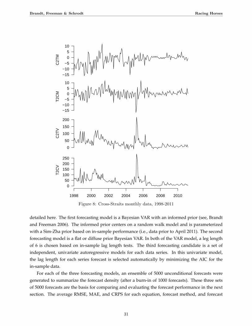
Brandt, Freeman & Schrodt Racing Horses
1998 2000 2002 2004 2006 2008 2010
−15
−10
−5
0
5
10
C2T
M
−15−10
−505
10
T2C
M
0
50
100
150
200
C2T
V
050
100150200250
T2C
V
Figure 8: Cross-Straits monthly data, 1998-2011
detailed here. The first forecasting model is a Bayesian VAR with an informed prior (see, Brandt
and Freeman 2006). The informed prior centers on a random walk model and is parameterized
with a Sim-Zha prior based on in-sample performance (i.e., data prior to April 2011). The second
forecasting model is a flat or diffuse prior Bayesian VAR. In both of the VAR model, a leg length
of 6 is chosen based on in-sample lag length tests. The third forecasting candidate is a set of
independent, univariate autoregressive models for each data series. In this univariate model,
the lag length for each series forecast is selected automatically by minimizing the AIC for the
in-sample data.
For each of the three forecasting models, an ensemble of 5000 unconditional forecasts were
generated to summarize the forecast density (after a burn-in of 1000 forecasts). These three sets
of 5000 forecasts are the basis for comparing and evaluating the forecast performance in the next
section. The average RMSE, MAE, and CRPS for each equation, forecast method, and forecast
31

Brandt, Freeman & Schrodt Racing Horses
horizon, relative to the true ex ante realizations of the data, are reported in Table 6. Entries in bold
are those that are considered “optimal” for each criteria. Several of the pitfalls of evaluating and
comparing forecasts that were discussed above become evident in this table.
First, the oft-heard time-series-forecasting mantra that univariate forecasts are superior to mul-
tivariate (system) forecasts is seen in the 6 and 12 period forecast comparisons across the models.
There is evidence that the RMSE and MAE are smaller for some or all of the series in the univariate
versus the BVAR models. As will be shown below, this is because these pooled univariate model
forecasts are overconfident and do not do a good job predicting events in the tail of the forecast
densities. Also, as the forecast horizon doubles, the “optimal” properties of the univariate-based
forecasts deteriorates since the multivariate BVAR models can better capture the important cross-
equation correlations that use this information to better predict the relevant time series.
However, a comparison of the conclusions from the equation-by-equation RMSE and MAE
statistics and the CRPS statistics leads to different conclusions. The CRPSs for the models indicate
that the forecast densities for the two BVAR models are superior for the C2TM and T2CM series
which summarize material conflict in the Straits. This is not the case for the two verbal conflict
zeries, where lower CRPSs are again observed in the univariate model. These failures in forecast-
ing coverage over the different horizons—which are the source of the results in Table 6—are more
evident in a graphical presentation of the forecasts and their error bands. Figure 9 presents the
three forecasts for each model over the two forecast horizons.
What becomes evident here is the same conclusions as Table 6: some of the forecasting models
do better than others for some of the variables. For instance, the two BVAR models have 68%
forecast intervals that cover the true data well for the C2TM and T2CM series, which is why these
have better CRPSs than those seen in the univariate model. The reverse is seen in the C2TV and
T2CV series, where there is evidence that the univariate forecasts have slightly better coverage
of the realized data. The forecast densities show us how and when these forecasting methods
succeed and fail. In the parlance of this paper, they tell us which horses are in the lead and by how
much.
The underlying issues in comparing the forecasting densities across the forecasting models
and horizons are ones of calibration and sharpness. Assessing the calibration and sharpness are
the job of the PIT and the VRH. Recall that the PIT measures how well the density of the forecasts
matches the actual density of the data. This is assessed using equation (17) from the earlier section.
Note however that in the present context, the forecast density is a three-dimensional object: a
multivariate prediction a series of conditional vectors over time. In terms of computing the PIT,
one can then marginalize the PIT density over the variables, time, etc. Since our interest is the
holistic evaluation of the forecasts, we choose the toughest case: the forecast density over the
entire six or twelve period forecast horizon (rather than one-step ahead at a time). This is a very
hard test since as Figure 9 already shows that the forecast density coverages are quite poor for
some of the variables for some of the models.
32

Brandt, Freeman & Schrodt Racing Horses
kM
od
elR
MS
EM
AE
CR
PS
C2T
MT
2C
MC
2TV
T2C
VC
2TM
T2C
MC
2TV
T2C
VC
2TM
T2C
MC
2TV
T2C
V
6B
VA
Rin
form
ed6.8
99.7
047
.30
38.5
75.
367.
3937
.21
29.6
81.72
2.19
11.0
78.98
6B
VA
Rfl
at6.8
111
.47
48.7
848
.70
5.31
8.87
37.9
236
.68
1.74
2.66
11.2
110
.89
6U
niv
aria
te2.39
3.07
10.01
9.71
1.70
2.80
9.07
7.80
3.93
7.23
6.01
9.38
12B
VA
Rin
form
ed7.47
10.72
52.4
245
.06
5.76
8.20
41.1
834
.90
1.75
2.41
12.2
710
.45
12
BV
AR
flat
7.4
612
.34
54.0
355
.56
5.80
9.58
42.2
942
.72
1.78
2.85
12.5
612
.78
12
Un
ivar
iate
20.
8432.
9820.69
38.63
16.1
926
.23
16.40
30.79
4.80
7.78
6.80
9.67
Tab
le6:
Per
form
an
ceof
the
thre
eC
ross
-str
aits
fore
cast
ing
mod
els
over
fore
cast
ing
hor
izon
k.
For
ecas
tev
alu
atio
ns
bas
edon
anen
sem
ble
of
5000
fore
cast
for
each
mod
elfo
rea
cheq
uat
ion
bas
edon
aver
age
Root
Mea
nS
qu
ared
Err
or(R
MS
E),
aver
age
Mea
nA
bso
lute
Err
or(M
AE
),an
dC
onti
nu
ou
sR
an
kP
rob
abil
ity
Sco
re(C
RP
S).
Entr
ies
inb
old
for
each
fore
cast
hor
izon
and
vari
able
are
con
sid
ered
“opti
mal
”.
33
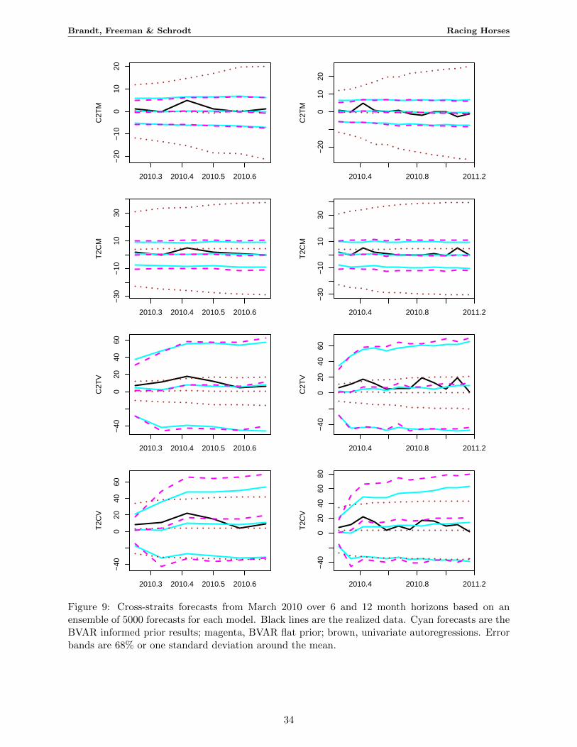
Brandt, Freeman & Schrodt Racing Horses
C2T
M
2010.3 2010.4 2010.5 2010.6
−20
−10
010
20
T2C
M
2010.3 2010.4 2010.5 2010.6
−30
−10
1030
C2T
V
2010.3 2010.4 2010.5 2010.6
−40
020
4060
T2C
V
2010.3 2010.4 2010.5 2010.6
−40
020
4060
C2T
M
2010.4 2010.8 2011.2
−20
010
20
T2C
M2010.4 2010.8 2011.2
−30
−10
1030
C2T
V
2010.4 2010.8 2011.2
−40
020
4060
T2C
V
2010.4 2010.8 2011.2
−40
020
4060
80
Figure 9: Cross-straits forecasts from March 2010 over 6 and 12 month horizons based on anensemble of 5000 forecasts for each model. Black lines are the realized data. Cyan forecasts are theBVAR informed prior results; magenta, BVAR flat prior; brown, univariate autoregressions. Errorbands are 68% or one standard deviation around the mean.
34

Brandt, Freeman & Schrodt Racing Horses
Figure 10 shows the PIT plots for each model over the 6 and 12 period forecast horizons. These
PIT values show the rather poor performance of the candidate forecasting models over the differ-
ent forecast horizons. Given the results of Table 6 this is to be expected: In each model at least one
of the series is poorly forecast, the forecast density matrix is mis-centered. This is clearly evident
in the PIT plots where we see a serious skew to he left and poor coverage in the middle and higher
parts of the forecast density.
The conclusion then from the earlier forecast density and now the PIT plots is that the BVAR
and univariate forecasts are poorly calibrated. This will also be evident when we look at the
combined calibration and sharpness in the VRH plots. Figure 11 plots the VRH for each model
and forecast horizon over the vector of forecast variables and periods. Here the relevant forecast
ensemble is the 5000 vectorized forecasts for the four variables over the forecast horizon (so the
length is 24 [48] for the 6 [12] period horizon) for each model. This gives us up to 24 ranked
forecasts for the 6 period model and up to 48 ranked forecasts for the 12 period model.
The VRH plot in Figure 11 gives the clearest explanation of the forecast performance over all
of the measures discussed. It shows which forecasts do better with respect to calibration and
sharpness. In the main, there is good evidence from the VRHs that the two BVAR forecasts are
well calibrated: the central tendencies of the VRHs for these models over both forecast horizons
are symmetric and correctly centered. The univariate forecast VRHs show that the forecast den-
sities from these models are off-center, or poorly calibrated (a fact already noted). What is more
important however, is that the univariate forecasts are very underdispersed. They are too con-
centrated and do not generate enough forecasts with low and high ranks compared to either the
BVAR-based models or the theoretical expectation of a uniform VRH. There is no evidence based
on a Komolgorov-Smirnov test that any of the VRHs in Figure 11 are uniform.
In terms of declaring a “winner” in this horserace, the conclusion is as nuanced as a horse
race handicapper would expect. Some horses are projected to run better on grass, others on turf.
Some horses do better in dry conditions and others when it rains. The odds-maker knows this
and can project winners using this information. Carrying this over to conflict forecasting for the
Cross-straits case, similar results are evident. First, using the RMSE or MAE criteria alone does
not properly assess the calibration or the sharpness of the forecasts. Second, the PIT only tells
us part of the story. Unlike in the mixture example, the Cross-Straits data shows that the way
we marginalize the PIT across variables and time does not make it apparent which forecast in
an ensemble is performing poorly. While we know from Figure 9 which models predict which
series better over each horizon, even a seemingly holistic assessment can confound forecast per-
formance. Finally, as the VRH plots illustrate, we can find some evidence that will let us handicap
the winners across forecasting models. The BVAR model performance is definitely superior to that
of the univariate models. This gives us a clear route to improving the forecast performance that
was not present in the comparisons of RMSE and MAE alone.
35
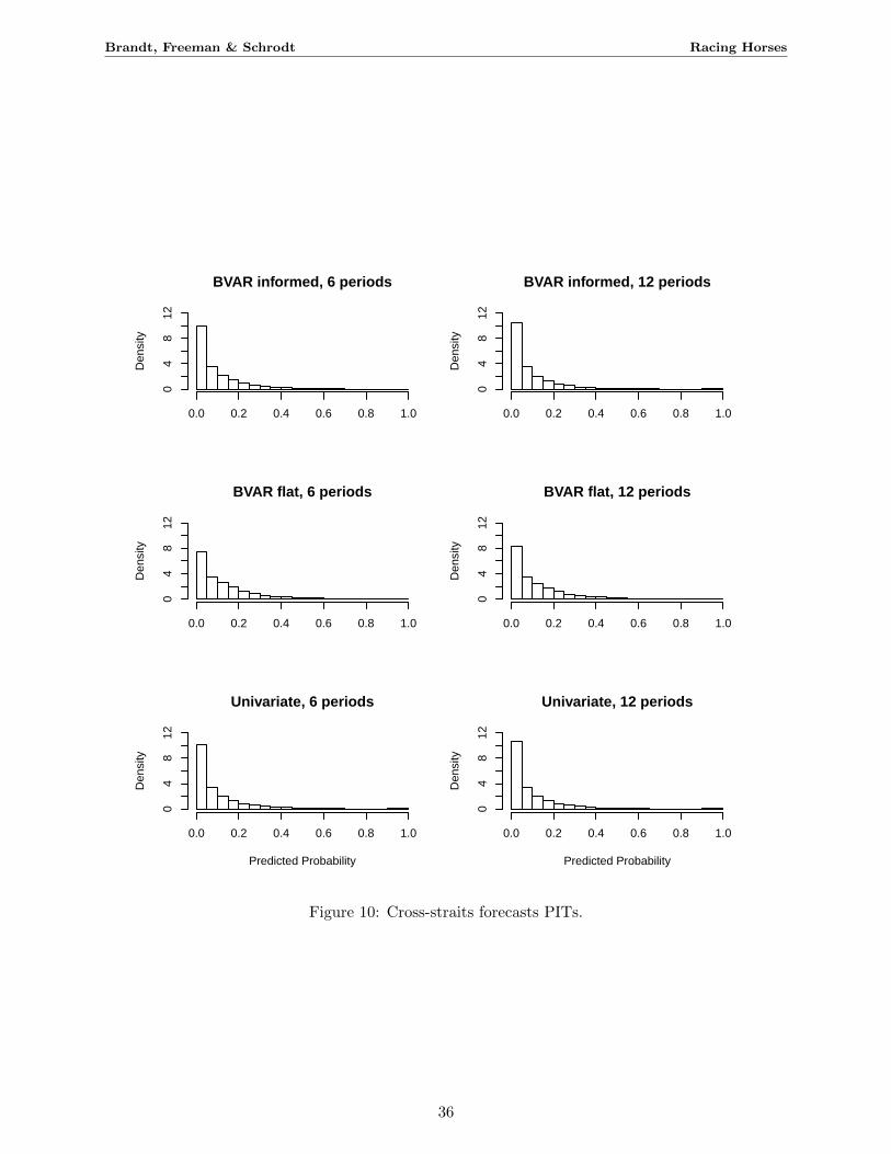
Brandt, Freeman & Schrodt Racing Horses
BVAR informed, 6 periods
Den
sity
0.0 0.2 0.4 0.6 0.8 1.0
04
812
BVAR flat, 6 periods
Den
sity
0.0 0.2 0.4 0.6 0.8 1.0
04
812
Univariate, 6 periods
Predicted Probability
Den
sity
0.0 0.2 0.4 0.6 0.8 1.0
04
812
BVAR informed, 12 periods
Den
sity
0.0 0.2 0.4 0.6 0.8 1.0
04
812
BVAR flat, 12 periods
Den
sity
0.0 0.2 0.4 0.6 0.8 1.0
04
812
Univariate, 12 periods
Predicted Probability
Den
sity
0.0 0.2 0.4 0.6 0.8 1.0
04
812
Figure 10: Cross-straits forecasts PITs.
36
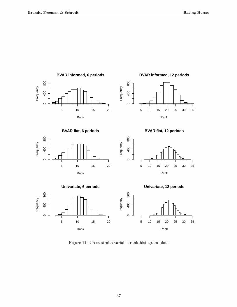
Brandt, Freeman & Schrodt Racing Horses
BVAR informed, 6 periods
Rank
Fre
quen
cy
5 10 15 20
040
080
0
BVAR flat, 6 periods
Rank
Fre
quen
cy
5 10 15 20
040
080
0
Univariate, 6 periods
Rank
Fre
quen
cy
5 10 15 20
040
080
0
BVAR informed, 12 periods
RankF
requ
ency
5 10 15 20 25 30 35
040
080
0BVAR flat, 12 periods
Rank
Fre
quen
cy
5 10 15 20 25 30 35
040
080
0
Univariate, 12 periods
Rank
Fre
quen
cy
5 10 15 20 25 30 35
040
080
0
Figure 11: Cross-straits variable rank histogram plots
37

Brandt, Freeman & Schrodt Racing Horses
6 Conclusion: Summary and Directions for Future Research
The pure and simple truth is rarely pure and never simple.
Oscar Wilde
In summary, we hope to have established three primary results in this paper. First, the so-
phisticated assessment of forecasts is important on both theoretical and practical grounds. For the
theoretical perspective, accurate forecasting is the defining characteristic of any scientific modeling
exercise. Models that are purely heuristic, explanatory or descriptive may have their place in our
academic discourse, but from the perspective of the philosophy of science, these are pre-scientificand as such indistinguishable from astrology, alchemy or mythology. Prediction is therefore some-
thing we need to take seriously.
However, because political science involves forecasting the behavior of complex, open sys-
tems, the models we will be evaluating are necessarily stochastic, and we are always making pre-
dictions about distributions, not points. This makes the problem of evaluating a prediction more
difficult than the predictions of deterministic systems—for example trying to predict the locations
of a comet and a spacecraft attempting to rendezvous with it—where simpler point predictions are
adequate. Despite this fact, unfortunately, there has been a tendency in political forecasting to use
methods such as RMSE and MAE which are more primarily useful in evaluating point predictions,
but, as we have demonstrated, can be quite misleading when used to evaluate distributions.
Second, by virtue of the fact that other fields—notably economics and meteorology– also have
dealt with predicting complex, open systems, there exists a rich set of tools for dealing with this
problem. We discussed a wide variety of these, along with some of their advantages and disad-
vantages. As is clear from that discussion, there is no single answer to this issue, and usually a
research will want to explore multiple indicators of forecasting accuracy.
Finally, we illustrate these issues both with idealized simulation results and with a compar-
ison of the results of multiple models that were used to model behavior in the China-Taiwan
“Cross-Straits” case. These examples demonstrate that the various measures can be used not only
to evaluate existing models, but also to provide guidance on how the models might be further
refined, for example by showing the existence of systematic bias and underdispersion in the es-
timates. These methods could be readily applied to other political forecasts, such as those of the
PITF, which are currently evaluated using point-prediction methods.
6.1 Summary of arguments and results
The use of a suite of tools in forecast evaluation
Directions for future research
-Spatial forecasting (see appendix)
-Teaming Horses–Model Pooling. Model ensembles in meteorology; ensemble Bayesian model
38

Brandt, Freeman & Schrodt Racing Horses
averaging (Raftery, et al. 2005, Berrocal et al 2007)Model averaging in macroeconomics (Geweke
and Amisano 2010) Model averaging in political science (Montgomery and Nylan 2010; Mont-
gomery, et al. 2011)
39
Brandt, Freeman & Schrodt Racing Horses
References
Abramowitz, Alan I. 2010 “How Large a Wave? Using the Generic Ballot to Forecast the 2010
Midterm Elections” PS: Political Science and Politics October: 631-632.Anderson, Jeffrey L. 1996. “A Method for Producing and Evaluating Probabilistic Forecasts from
Ensemble Model Integrations.” Journal of Climate 9: 1518-1530.Armstrong, J. Scott, Editor. 2001 Principles of Forecasting: A Handbook for Researchers and Practioneers
Boston: Kluwer Publishers.Armstrong, J.Scott and Fred Collopy. 1992 “Error Measures for Generalizing About Forecasting
Methods: Empirical Comparisons” International Journal of Forecasting 8(1): 69-80.Aron, Janine and John Meulbauer. 2010. “New Methods for Forecasting Inflation, Applied to the
U.S.” Discussion paper no. 7877. Centre for Economic Policy Research (CEPR). Oxford.Austen-Smith, David and Jeffrey Banks. 1996. “Information Aggregation, Rationality, and the
Condorcet Jury Theorem” The American Political Science Review 90(1): 34-45.Berrocal, Veronica J., Adrian E. Raftery, and Tilman Gneiting. 2007. ”Combining Spatial Statis-
tical and Ensemble Information in Probabilistic Weather Forecasts.” Monthly Weather Review135(April): 1386-1402.
Bafumi, Joseph, Robert S.Erikson, and Christopher Wlezien, 2010. ”Forecasting House Seats from
Generic Congressional Polls: The 2010 Midterm Elections” PS: Political Science and Politics Oc-
tober: 633-636.Beck, Nathaniel. 2000. “Evaluating Forecasts and Forecasting Models of the 1996 Presidential
Election.” In Before the Vote: Forecasting American National Elections James E. Campbell and
James C. Garand (eds.). Thousand Oaks, Ca.: Sage Publications, Inc.Beck, Nathaniel, Gary King, and Langche Zeng. 2000. “Improving Quantitative Studies of Inter-
national Conflict: A Conjecture.” American Political Science Review 94: 21-36.Bagozzi, Benjamin 2011. “Forecasting Civil Conflict with Zero-Inflated Count Models.” Manuscript.
Pennsylvania State University.Bueno de Mesquita, Bruce. 2010. “A New Model for Predicting Policy Choices: Prelminary Tests”
Conflict Management and Peace ScienceBrandt, Patrick T., John R. Freeman, and Philip A. Schrodt. 2010. ”Real Time, Time Series Fore-
casting of Inter- and Intra-state Political Conflict” Conflict Management and Peace ScienceBrandt, Patrick T. and John R. Freeman. 2009. ”Modeling Macro Political Dynamics.” Political
Analysis 17:113-142.Brandt, Patrick T., Michael Colaresi, and John R. Freeman. 2008. “The Dynamics of Reciprocity,
Accountability and Credibility.” Journal of Conflict Resolution 52(3): 343-374.Brandt, Patrick T. and John R. Freeman. 2006. “Advances in Bayesian Time Series Modeling and
the Study of Politics: Theory Testing, Forecasting and Policy Analysis” Political Analysis 14(1):
1-36.Campbell, James E. 2000. ”The Science of Forecasting Presidential Elections.” In Before the Vote:
Forecasting American National Elections, James E. Campbell and James C. Garand (eds.). Thou-
sand Oaks, Ca.: Sage Publications, Inc.
40

Brandt, Freeman & Schrodt Racing Horses
Campbell, James E. 2010a. “Forecasting of the 2010 Midterm Elections: Editor’s Introduction” PS:Political Science and Politics October: 625-626.
Campbell, James E. 2010b. “Seats in Trouble Forecast of the 2010 Elections to the U.S. House” PS:Political Science and Politics October: 627-630.
Chaloner, Kathryn M., Timothy Church, Thomas A. Louis, and John P. Matts. 1993. “Graphical
Elicitation of a Prior Distribution for a Clinical Trail.” The Statistician 42(4): 341-53.Chaloner, Kathryn M., and G. T. Duncan. 1983. “Assessment of a Beta Prior Distribution: PM
Elicitation.” The Statistician 32(1/2): 174-80.Chatfield, Chris. 1993. “Calculating Interval Forecasts” Journal of Business and Economic Statistics
11(2): 121-135.Chatfield, Chris 2001 “Prediction Intervals for Time-Series Forecasting.” In Principles of Forecasting:
A Handbook for Researchers and Practioneers J. Scott Armstrong Ed. Boston: Kluwer.Christoffersen, Peter F. 1998. “Evaluating Interval Forecasts.” International Economic Review 39(4):
841-862.Clements, Michael P. and Jeremy Smith. 2000. “Evaluating the Forecast Densities of Linear and
Non-Linear Models; Applications to Output Growth and Unemployment” Journal of Forecast-ing 19: 255-276.
Clements, Michael P. and David F. Hendry, 1998 Forecasting Economic Time Series NY: Cambridge
University Press.Cuzan, Alfred G. 2010. “Will the Republicans Retake the House in 2010?” PS: Political Science and
Politics October: 639-641.
bibitem Dawid, A. P. 1984. “Statistical Theory: A Prequential Approach.” Journal of the RoyalStatistical Society Ser. A. 147: 278-292.Dhyrmes, P. J., et al. 1972 “Criteria for Evaluation of Econometric Models.” Annals of Economic and
Social Measurement 1: 291-334.Diebold, Francis X., Jinyong Hahn, and Anthony S. Tsay. 1999. “Multivariate Density Forecast
Evaluation and Calibration in Financial Risk Management: High Frequency Returns on For-
eign Exchange.” The Review of Economics and Statitics 81(4): 661-673.Diebold, Francis X., Todd A. Gunther, and Anthony S. Tay. 1998. “Evaluating Density Forecasts
With Applications to Financial Risk Management.” International Economic Review 39(4): 863-
883.Doan, Thomas, Robert Litterman, and Christopher Sims. 1984 “Forecasting and Condition Projec-
tions Using Realistic Prior Distributions.” Econometric Reviews 3:1-100.Enders, Walter. 2010 Applied Time Series Analysis NY. Wiley.Fearon, James and David Laitin. 2003. “Ethnicity, Insurgency, and Civil War.” American Political
Science Review 97: 75-90.Fildes, Robert and Herman Stekler 2002. “The State of Macroeconomic Forecasting” Journal of
Macroeconomics 24: 435-468Fildes, Robert (Editor) 1995. World Index of Economic Forecasts Fourth Edition. U.K.: Gower, Alder-
shot, and Hampshire.
41

Brandt, Freeman & Schrodt Racing Horses
Fraley, Chris, Adrian E. Raftery, Tilman Gneiting, and J. McLean Sloughter. 2009. “EnsembleBMA:
An R Package for Probabilistic Forecasting using Ensembles and Bayesian Model Averaging.”
Technical Report no. 516R. Department of Statistics, University of Washington. Seattle, Wash-
ington.Freeman, John R. and Jeff Gill. 2010. “Dynamic Elicited Priors for Updating Covert Networks.”
Manuscript. Washington University-St. Louis.Freeman, John R., Jude C. Hays, and Helmut Stix. 2000. “Democracy and Markets: The Case of
Exchange Rates.” The American Journal of Political Science 44(3): 449-468. Working paper number
39. Working paper series of the Austrian National Bank.Freeman, John R., John T. Williams and Tse-min Lin. 1989. “Vector Autoregression and the Study
of Politics” American Journal of Political Science 33:842-877.Garratt, Anthony and Shawn P. Vahey. 2006. “UK Real-Time Macro Data Characteristics.” The
Economic Journal 116: F119-F135.Garthwaite, Paul H., Joseph B. Kadane, and Anthony O’Hagan. 2005. “Statistical Methods for
Eliciting Probability Distributions.” Journal of the American Statistical Association 100(170): 680-
700.Geweke, John and Gianni Amisano. 2009. ”Optimal Prediction Pools.” Working paper no. 1017.
European Central Bank. Frankfurt, Germany.Gerner, Deborah J. and Philip A. Schrodt and Omur Yilmaz. 2009 Conflict and Mediation Event
Observations (CAMEO) Codebook http://eventdata.psu.edu/data.dir/cameo.htmlGill, Jeff and Walker, Lee. 2005. “Elicited Priors for Bayesian Model Specifications in Political
Science Research.” Journal of Politics 67, 841-872.Gneiting, Tilman. 2008. “Editorial: Probabilistic Forecasting.” Journal of the Royal Statistical Society
A, 172, Part 2: 319-321.Gneiting, Tilman, Fadoua Balabdaoui, and Adrian E. Raftery. 2007. “Probabilistic Forecasts, Cali-
bration and Sharpness.” Journal of the Royal Statistical Society 69(Pt.2): 243-268.Gneiting, T., K. Larson, K. Westrick, M. G. Genton, E. Aldrich. 2006. “Calibrated probablistic fore-
casting at the Stateline wind energy centre: the regime-switching space-time (RST) method.”
Journal of the American Statistical Association 101: 968-979.Gneiting, T. and A. Raftery. 2006. “Strictly Proper Scoring Rules, Prediction and Estimation.”
Journal of the American Statistical Association 102(477): 359-378.Gneiting, Tilman and Adrian E. Raftery. 2005. “Weather Forecasting with Ensemble Methods.”
Science 310(October)248-249.Goldstone, Jack A., Robert H. Bates, David L. Epstein, Ted Robert Gurr, Michael B. Lustik, Monty
G. Marshall, Jay Ulfelder, and Mark Woodward. 2010. ”A Global Model for Forecasting Politi-
cal Instability.” American Journal of Political Science 54(1): 190-208.Good, I.J. 1952. “Rational Decisions.” Journal of the Royal Statistical Society Ser. B, 14: 107-114.Grell, Georg A., Jimy Dudhia, and David R. Stauffer. 1995. A Description of the Fifth-Generation Penn
State/ NCAR Mesoscale Model (MM5) NCAR/TN-398+STR National Center for Atmospheric
Research: Boulder, CO.
42
Brandt, Freeman & Schrodt Racing Horses
Grimit, Eric P. and Clifford F. Mass. 2002. “Initial Results of a Mesoscale Short-Range Ensemble
Forecasting System over the Pacific Northwest.” Weather and Forecasting 17(April): 192-205.Hamill, Thomas M. 2001. “Notes and Correspondence. Interpretation of Rank Histograms for
Verifying Ensemble Forecasts.” Monthly Weather Review 129: 550-560.Hays, Jude C., John R. Freeman, and Hans Nesseth. 2003. “Exchange Rate Volatility and Democ-
ratization in Emerging Market Countries.” International Studies Quarterly 47(2): 203-228.Hersbach, Hans. 2000. ”Decomposition of the Continuous Ranked Probability Score for Ensemble
Prediction Systems” Weather and Forecasting 15(October): 559-570.Huth, Paul K. and Todd L. Allee. 2002a. “Domestic Political Accountability and the Escalation
and Settlement of International Disputes.” Journal of Conflict Resolution 46(6): 754-790.Huth, Paul K. and Todd L. Allee. 2002b. The Democratic Peace and Territorial Conflict in the Twentieth
Century Ann Arbor, MI. University of Michigan Press.Kadane, Joseph B., and Lara J. Wolfson. 1998. “Experiences in Elicitation.” Journal of The Royal
Statistical Society, Series D 47(1): 3-19.Keashly, L. and R. J. Fisher. 1996. “A Contingency Perspective on Conflict Interventions: Theo-
retical and Practical Considerations.” Resolving International Conflict: The Theory and Pratice ofMediation
King, Gary and Langche Zeng. 2001. “Improving Forecasts of State Failure.” World Politics 53:
623-658.Kling, John L. and David A. Bessler. 1989. “Calibration-based Predictive Distributions: An Appli-
cation of Prequential Analysis to Interest Rates, Money, Prices, and Output.” Journal of Business62(4): 477-499.
Klarner, Carl. 2010 “Forecasting the 2010 State Legislative Elections” PS: Political Science and Poli-tics October: 643-648.
Kmenta, J. 1986. Elements of Econometrics New York: Macmillan.Lebovic, James H. 1995. “How Organizations Learn: U.S. Government Estimates of Foreign Mili-
tary Spending.” American Journal of Political Science 39, 4:835-863.Lewis-Beck, Michael S. and Charles Tien. 2010. ”The Referendum MOdel: A 2010 Congressional
Forecast” PS: Political Science and Politics October: 637-638.Lewis-Beck, Michael s. and Charles Tien. 2000. “The Future of Forecasting: Prospective Presiden-
tial Models.” In Before the Vote: Forecasting American National Elections James E. Campbell and
James C. Garand editors. Sage Publications.Leamer, Edward E. 1992. “Bayesian Elicitation Diagnostics.” Econometrica 60(4): 919-42.Litterman, Robert B. 1986. “Forecasting with Bayesian Vector Autoregressions–Five Years of Ex-
perience.” Journal of Business, Economics and Statistics 4:25-38.Lutepohl, Helmut. 2006 New Introduction to Multiple Time Series Analysis Berlin: Springer.Makridakis, S., A. Andersen, R. Carbone, R. Fildes, Hibon, R. Lewandowski, J. Newton, E. Parzen,
and R. Winkler. 1982. “The Accuracy of ExtrapolationTime Series Methods: Results of a Fore-
casting Competition.” Journal of Forecasting 1: 111-153.Matheson, James E. and Robert L. Winkler. 1976. “Scoring Rules for Continous Probability Distri-
butions.” Management Science 22(10): 1087-1096.
43
Brandt, Freeman & Schrodt Racing Horses
Montgomery, Jacob M. and B. Nyhan. 2010. “Bayesian Model Averaging: Theoretical Develop-
ments and Practical Applications.” Political Analysis 18(2): 245-270.Montgomery, Jacob M., Florian Hollenbach, and Michael D. Ward. 2011. “Improving Predictions
Using Ensemble Bayesian Model Averaging” Manuscript. Duke University.Murphy, Allan H. 1972a. “Scalar and Vector Partitions of the Probability Score: Part I: Two State
Situation.” Journal of Applied Meterology 11(March): 273-282.Murphy, Allan H. 1972b. “Scalar and Vector Partitions of the Probability Score: Part II. N-State
Situations.” Journal of Applied Meterology 11(December):1183-1192.Murphy, Allan H. and Robert Winkler. 1974 “Subjective Probability Forecasting Experiments in
Meterology: Some Preliminary Results” Bulletin of the American Meterological Society 55(10):
1206-1216.O’Brien, Sean. 2010. “Crisis Early Warning and Decision Support: Contemporary Approaches
and Thoughts on Future Research.” International Studies Review 12,1: 87-104.O’Hagan, A. 1998. “Eliciting Expert Beliefs in Substantial Practical Applications.” The Statistician
47, 21-35.Park, Jong Hee. 2010. “Structural Change in the the U.S. Presidents’ Use of Force Abroad.” Amer-
ican Journal of Political Science 54(3): 766-782.Pearson, K. 1933 “On a method of determining whether a sample of size n supposed to have been
drawn from a parent population having a known probability integral has probably been drawn
at random.” Biometrika 25: 379-410.Pindyck, Robert S. and Daniel L. Rubinfeld. 1998. Econometric Models and Economic Forecasts Fourth
Edition. New York: MacGraw Hill, Inc.Raftery, Adrian E., Tilman Gneiting, Fadoua Balabdaoui, Michael Polakowski. 2005. “Using
Bayesian Model Averaging to Calibrate Forecast Ensembles.” Monthly Weather Review 133
(May):1155-1174.Rioux, Jean-Sebastien 1998. “A Crisis-Based Evaluation of the Democratic Peace Propositions.”
Canadian Journal of Political Science 31(2): 263-283.Robertson, John C. and Ellis Tallman. 1999. “Vector Autoregressions: Forecasting and Reality.”
Economic Review(Atlanta Federal Reserve Bank) 84(4):4-18.Rosenblatt, M. 1952. “Remarks on a Multivariate Transformation” Annals of Mathematical Statistics
23: 470-472.Rousseau, David L. 2005. Democracy and War: Institutions, Norms, and the Evolution of International
Conflict Stanford, CA. Stanford University Press.Sattler, Thomas, Patrick T. Brandt, and John R. Freeman. 2010. “Democratic Accountability in
Open Economies.” The Quarterly Journal of Political Science 5: 71-97.Schrodt, Philip A. 2010. “Seven Deadly Sins of Contemporary Quantitative Analysis.” Presented
at the American Political Science Association meetings, Washington.Schrodt, Philip A. 2011. “Forecasting Political Conflict in Asia Using Latent Dirichlet Allocation
Models.” Paper presented at the Annual Meeting of the European Political Science Association,
Dublin.
44

Brandt, Freeman & Schrodt Racing Horses
Schrodt, Philip A. and Deborah Gerner. 2000. “Cluster Based Early Warning Indicators for Politi-
cal Change in the Contemporary Levant.” American Political Science Review 94(4): 803-818.Seidenfeld, Tony. 1985. “Calibration, Coherence, and Scoring Rules.” Philosphy of Science 52: 274-
294.Senese, Paul D. and John A. Vasquez. 2008. The Steps to War: An Empirical Study Princeton, NJ.
Princeton University Press.Sims, Christopher A. 2005. “The State of Macroeconomic Policy Modeling: Where Do We Go From
Here?” Macroeconomics and Reality Twenty Five Years Later Conference, Barcelona, Spain.Sims, Christopher A. 1986. “Are Forecasting Models Useful For Policy Analysis.” Quarterly Review
Minneapolis, MN. Federal Reserve Bank of Minneapolis 10: 2-16.Sims, Christopher A. and Tao A. Zha 1998. “Bayesian Methods for Dynamic Multivariate Models.”
International Economic Review 39(4):949-968.Sing, Tobias, Oliver Sander, Niko Beerenwinkel and Thomas Lengauer. 2009. Package ROCR: Visu-
alizing the performance of scoring classifiers. Available at http://cran.r-project.org/web/packages/ROCR/
Version dated 08-Dec-2009.Smets, Frank and Rafael Wouters. 2007. “Shocks and Frictions in U.S. Business Cycles: A Bayesian
DSGE Approach” American Economic Review 97(3):586-606.Surowiecki, J. 2004. The Wisdom of Crowds: Why the Many are Smarter than the Few and Collective
Wisdom Shapes Business, Economics Societies and Nations New York: Doubleday.Tay, Anthony S. and Kenneth F. Wallis. 2000. “Density Forecasting: A Survey” Journal of Forecasting
19: 235-254.Taylor, J.w. 1999. “Evaluating Volatility and Interval Forecasts.” Journal of Forecasting 18: 111-128.Tetlock, Phillip. 2006. Expert Political Judgment: How Good is It? How Can We Know? Princeton:
Princeton University Press.Thiel, Henri. 1966 Applied Economic Forecasting Amsterdam: North-Holland.Timmerman, Allan. 2000. “Density Forecasting in Economics and Finance.” Journal of Forecasting
19: 231-234.Treier, Shawn and Simon Jackman. 2008. “Democracy as a Latent Variable.” American Journal of
Political Science 52(1): 201-217.Weigend, Andreas S. and Shanming Shi. 2000. “Predicting Daily Probability Distributions of S&P
Returns.” Journal of Forecasting 19: 375-392.Wieland, Volker and Maik H. Wolters. 2010. “The Diversity of Forecasts From Macroeconomic
Models of the U.S. Economy.” Discussion paper no. 7870. Centre for Economic Policy Research
(CEPR). Oxford.Winkler, Robert L. 1969. ”Scoring Rules and the Evaluation of Probability Assessors.” American
Statistical Association Journal September: 1073-1078.Winkler, Robert L. and Allan H. Murphy. 1968. “’Good’ Probability Assessors.” Journal of Applied
Meteorology 7(October): 751-758.Wolfers, Justin and Eric W. Zitzewitz. 2004. “Prediction Markets” Journal of Economic Perspectives
18(2): 107-126.
45

Brandt, Freeman & Schrodt Racing Horses
Appendix
Evaluation Metrics. Formulae
The notation is as follows: 55
m: forecasting method
rw: random walk model
h: forecast horizon
s: series being forecast
F: a forecast of a variable
A: actual value (realization) of a variable
H: the number of horizons to be forecast
S: number of series being forecast.
So, for example, Fm,h,s using the forecast for method m at horizon h for series s.
The absolute percentage error (APE) is defined as
APEm,h,s = |Fm,h,s −Ah,s
Ah,s|. (21)
Using this defintion, we can construct formulae for the mean absolute error, MAPE, and Median
absolute error, MdAPE:
MAPEm,h =
∑Ss=1APEm,h,s
Sx100; (22)
For rank ordered APEm,h,s values, MdAPEm,h = the ranked value S+12 if S is odd or the mean
of values S2 and S
2 + 1 if S is even.
Relative absolute error, RAE, is defined as
RAEm,h,s =|Fm,h,s −Ah,s||Frw,h,s −Ah,s|
(23)
where the benchmark model is the random walk hence the use of Frw,h,s in the denominator.56
The geometric mean of the relative absolute forecast error is expressed as
GMRAEm,h = [ΠSs=1RAEm,h,s]
1s (24)
whereas the median relative absolute forecast error is defined like the MdAPE. We first rank
the values of the RAEm,h,s. Then MdRAEm,h = the value S+12 if S is odd and the mean of the
values S2 and S
2 + 1 if S is even.
There are several measures of RAE for the cumulative performance of a model across multiple
55This summary is a condensed version of the appendix in Armstrong and Collopy (1992: 78-79)56Recall from footnote 22 in the text that the forecast function for the pure random walk is flat at any time t.
46
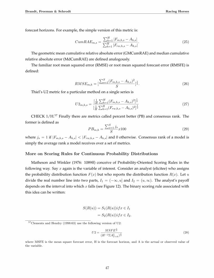
Brandt, Freeman & Schrodt Racing Horses
forecast horizons. For example, the simple version of this metric is:
CumRAEm,s =
∑Hh=1 |Fm,h,s −Ah,s|∑Hh=1 |Frw,h,s −Ah,s|
. (25)
The geometric mean cumulative relative absolute error (GMCumRAE) and median cumulative
relative absolute error (MdCumRAE) are defined analogously.
The familiar root mean squared error (RMSE) or root mean squared forecast error (RMSFE) is
defined:
RMSEm,h = [
∑Ss=1(Fm,h,s −Ah,s)
2
S]12 . (26)
Thiel’s U2 metric for a particular method on a single series is
U2m,h,s =[ 1H
∑Hh=1(Fm,h,s −Ah,s)
2]12
[ 1H
∑Hh=1(Frw,h,s −Ah,s)2]
12
(27)
CHECK 1/H.57 Finally there are metrics called percent better (PB) and consensus rank. The
former is defined as
PBm,h =
∑Ss=1 jsS
x100 (29)
where js = 1 if |Fm,h,s − Ah,s| < |Frw,h,s − Ah,s| and 0 otherwise. Consensus rank of a model is
simply the average rank a model receives over a set of metrics.
More on Scoring Rules for Continuous Probability Distributions
Matheson and Winkler (1976: 1089ff) conceive of Probability-Oriented Scoring Rules in the
following way. Say x again is the variable of interest. Consider an analyst (elicitee) who assigns
the probability distribution function F (x) but who reports the distribution function R(x). Let u
divide the real number line into two parts, I1 = (−∞, u] and I2 = (u,∞). The analyst’s payoff
depends on the interval into which x falls (see Figure 12). The binary scoring rule associated with
this idea can be written:
S(R(u)) = S1(R(u))ifx ∈ I1= S2(R(u))ifx ∈ I2.
57Clements and Hendry (1998:63) use the following version of U2:
U2 =MSFE
12
(H−1ΣA2T+h)
12
(28)
where MSFE is the mean square forecast error, H is the forecast horizon, and A is the actual or observed value ofthe variable.
47

Brandt, Freeman & Schrodt Racing Horses
Figure 12: Probability Oriented Scoring Rules. Source: Matheson and Winkler 1967: Figure 1
The expected value of the predictive distribution reported by the analyst is:
E(S(R(u))) = F (u)S1(R(u)) + [1-F(u)]S2(R(u)).
And the key to showing a scoring rule is proper is to demonstrate that the assigned predic-
tive distribution yields an expected value greater or equal to any revealed predictive distribution.
Hence the analyst has no incentive to hedge.
To generalize this framework, Matheson and Winkler that there is a probability distribution,
G(u), for the cut point that defines the two intervals. This produces an expected score once x is
realized of:
S**(R(.))=Eu|x(S(R(u))) =∫ x
−∞S2(R(u))dG(u) +
∫ ∞xS1(R(u))dG(u).
Before x is realized, the analyst’s expected score is:
E(S∗∗(R(.))) =
∫ ∞−∞
E(S(R(u)))dG(u).
For instance, the payoff for the continuous quadratic rule can now be rewritten:
S∗∗(R(.)) = −∫ x
−∞R2(u)dG(u)−
∫ ∞x
[1−R(u)]2dG(u).
The expected score for this case is:
48
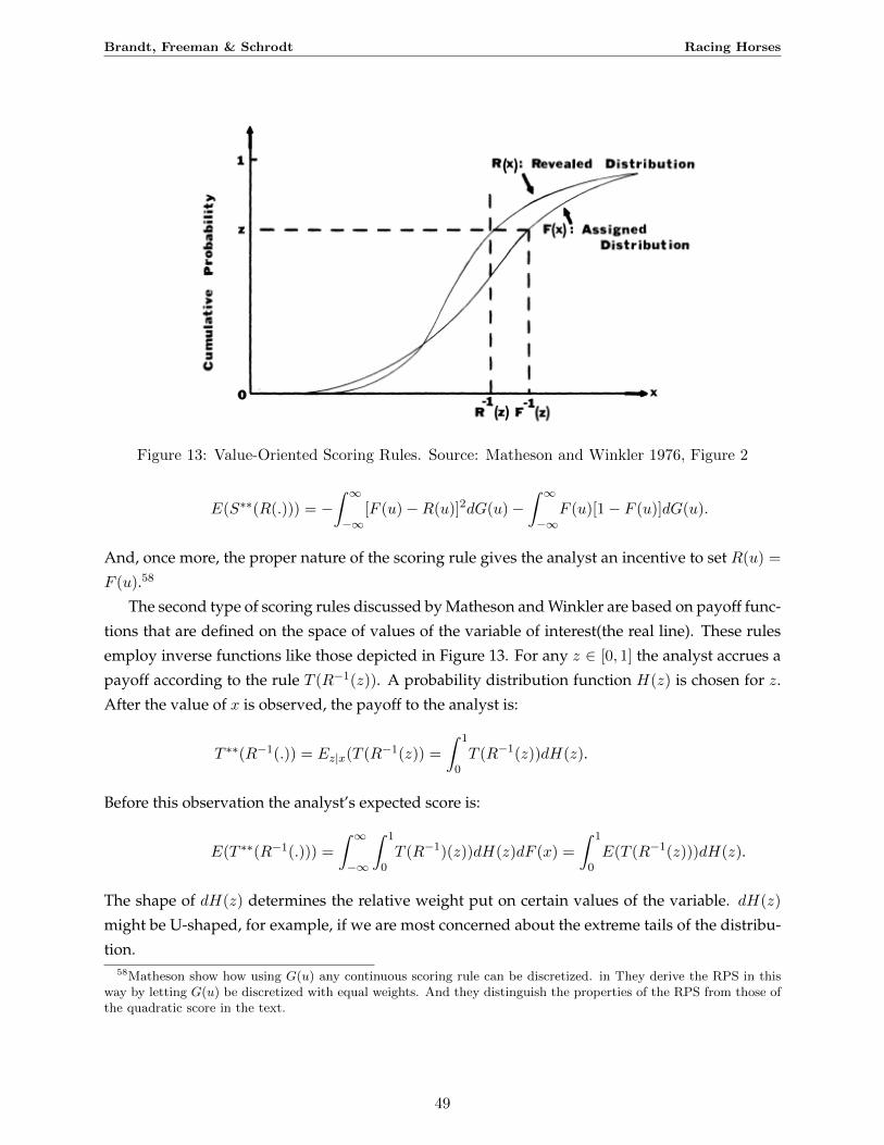
Brandt, Freeman & Schrodt Racing Horses
Figure 13: Value-Oriented Scoring Rules. Source: Matheson and Winkler 1976, Figure 2
E(S∗∗(R(.))) = −∫ ∞−∞
[F (u)−R(u)]2dG(u)−∫ ∞−∞
F (u)[1− F (u)]dG(u).
And, once more, the proper nature of the scoring rule gives the analyst an incentive to set R(u) =
F (u).58
The second type of scoring rules discussed by Matheson and Winkler are based on payoff func-
tions that are defined on the space of values of the variable of interest(the real line). These rules
employ inverse functions like those depicted in Figure 13. For any z ∈ [0, 1] the analyst accrues a
payoff according to the rule T (R−1(z)). A probability distribution function H(z) is chosen for z.
After the value of x is observed, the payoff to the analyst is:
T ∗∗(R−1(.)) = Ez|x(T (R−1(z)) =
∫ 1
0T (R−1(z))dH(z).
Before this observation the analyst’s expected score is:
E(T ∗∗(R−1(.))) =
∫ ∞−∞
∫ 1
0T (R−1)(z))dH(z)dF (x) =
∫ 1
0E(T (R−1(z)))dH(z).
The shape of dH(z) determines the relative weight put on certain values of the variable. dH(z)
might be U-shaped, for example, if we are most concerned about the extreme tails of the distribu-
tion.58Matheson show how using G(u) any continuous scoring rule can be discretized. in They derive the RPS in this
way by letting G(u) be discretized with equal weights. And they distinguish the properties of the RPS from those ofthe quadratic score in the text.
49

Brandt, Freeman & Schrodt Racing Horses
Figure 14: Continuous Analogue of the VRH. Source: Gneiting et al 2005
The Continuous Analogue of the VRH
Proponents of probabilistic forecasting sometimes use the continuous analogue of the VRH. In
fact, they sometimes use both forms of the VRH in the same article (Raftery, et al. 2005). This form
emerges from histogram density estimation (Diebold et al 1999: 664). Figure GG is an illustration.
The key difference between the two versions of the VRH are the scales on the vertical axis (cf.
Figure 6 in the text). For the continuous analogue, the area of each triangle represents the relative
frequency of truth appearing the respective rank. If the unit interval is divided into say 10 bins
(ranks), as in Figure 14 above, the width of the bottom parts of these rectangles is always 0.10.
So say that 100 forecasts are made and that the observed values end up in the first rank 10 times.
Then the relative frequency is 10100 = 0.10. To depict this frequency, the rectangle will have height 1
so the area covered by the first bin is 1× 0.10 = 0.10. Alternatively, say that the forecast ensemble
has too little variability and the observations end up in the first rank 15 times so that that rank one
has relative frequency 0.15. Then the first rectangle in the continuous analogue VRH would have
height 1.5 so that its area is 1.5× 0.10 = 0.15.
Spread error plots such as those shown in Figure 15 are used to assess skill of forecasting
ensembles.They are used in model averaging. It is possible for ensembles to evidence forecasting
skill but still be uncalibrated (see Raftery, et al. 2005: 1155-1156. See also Grimit and Mass 2002).
A Note on Spatial Forecasting
Atmospheric analysis is necessarily three dimensional. the relevant models relate physical
forces like wind speed and temperature at different places and at different levels of the atmo-
sphere. For example, vertical diffusion is a key component of the MM5 model. Meteorological
50
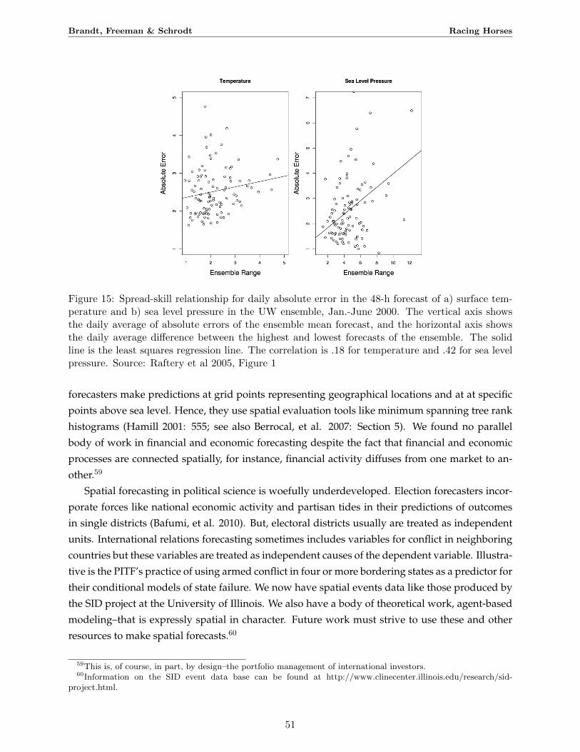
Brandt, Freeman & Schrodt Racing Horses
Figure 15: Spread-skill relationship for daily absolute error in the 48-h forecast of a) surface tem-perature and b) sea level pressure in the UW ensemble, Jan.-June 2000. The vertical axis showsthe daily average of absolute errors of the ensemble mean forecast, and the horizontal axis showsthe daily average difference between the highest and lowest forecasts of the ensemble. The solidline is the least squares regression line. The correlation is .18 for temperature and .42 for sea levelpressure. Source: Raftery et al 2005, Figure 1
forecasters make predictions at grid points representing geographical locations and at at specific
points above sea level. Hence, they use spatial evaluation tools like minimum spanning tree rank
histograms (Hamill 2001: 555; see also Berrocal, et al. 2007: Section 5). We found no parallel
body of work in financial and economic forecasting despite the fact that financial and economic
processes are connected spatially, for instance, financial activity diffuses from one market to an-
other.59
Spatial forecasting in political science is woefully underdeveloped. Election forecasters incor-
porate forces like national economic activity and partisan tides in their predictions of outcomes
in single districts (Bafumi, et al. 2010). But, electoral districts usually are treated as independent
units. International relations forecasting sometimes includes variables for conflict in neighboring
countries but these variables are treated as independent causes of the dependent variable. Illustra-
tive is the PITF’s practice of using armed conflict in four or more bordering states as a predictor for
their conditional models of state failure. We now have spatial events data like those produced by
the SID project at the University of Illinois. We also have a body of theoretical work, agent-based
modeling–that is expressly spatial in character. Future work must strive to use these and other
resources to make spatial forecasts.60
59This is, of course, in part, by design–the portfolio management of international investors.60Information on the SID event data base can be found at http://www.clinecenter.illinois.edu/research/sid-
project.html.
51