1

PaToPa: A Data-Driven Parameter and TopologyJoint Estimation Framework in Distribution Grids

Jiafan Yu, Student Member, IEEE, Yang Weng, Member, IEEE, Ram Rajagopal, Member, IEEE

Abstract—The increasing integration of distributed energyresources (DERs) calls for new planning and operational tools.However, such tools depend on system topology and line pa-rameters, which may be missing or inaccurate in distributiongrids. With abundant data, one idea is to use linear regression tofind line parameters, based on which topology can be identified.Unfortunately, the linear regression method is accurate only ifthere is no noise in both the input measurements (e.g., voltagemagnitude and phase angle) and output measurements (e.g.,active and reactive power). For topology estimation, even witha small error in measurements, the regression-based method isincapable of finding the topology using non-zero line parameterswith a proper metric. To model input and output measurementerrors simultaneously, we propose the error-in-variables (EIV)model in a maximum likelihood estimation (MLE) frameworkfor joint line parameter and topology estimation. While directlysolving the problem is NP-hard, we successfully adapt theproblem into a generalized low-rank approximation problem viavariable transformation and noise decorrelation. For accuratetopology estimation, we let it interact with parameter estimationin a fashion that is similar to expectation-maximization fashionin machine learning. The proposed PaToPa approach does notrequire a radial network setting and works for mesh networks.We demonstrate the superior performance in accuracy for ourmethod on IEEE test cases with actual feeder data from SouthCalifornia Edison.

I. INTRODUCTION

Electric grids are undergoing a revolution towards a moresustainable system. Renewables and other distributed energyresources (DERs) are expected to supply more than 50%of electricity demand by 2050 [?], [?]. While adding newcapabilities, DER penetration raises significant concern aboutthe resilience of power grids, especially in distribution grids.This is because DERs create two-way power flows, whichnegatively impact the stability of distribution grids. Therefore,efficient planning and operational tools are needed for DERsin distribution grids.

Unfortunately, the prerequisite of such planning and op-erational tools may not be satisfied in current distributiongrids. Different from transmission grids, where the topologiesand line parameters are regularly measured and verified, suchsystem information in distribution grids can be inaccurate oreven unavailable. This is because the line parameter profilesin distribution grids are usually only available from gridplanning files and the nameplate values, which are likely to beoutdated. For example, many substation engineers find it hard

J. Yu and R. Rajagopal are with Stanford University, Stanford, CA, 94305USA. e-mail: {jfy, ramr}@stanford.edu

Y. Weng is with Arizona State University, Tempe, AZ, 85287 USA. e-mail:yang.weng@asu.edu

to construct the admittance matrix when using distributionmanagement systems, such as CYME [?]. Furthermore, inmany secondary distribution grids, the topology information isfrequently missing. Finally, the measurement and verificationtools are limited in distribution grids, making it hard forsystem operators to track the updates of the line connections,e.g., the real-time switches in distribution grids. Withoutaccurate topology and line parameters, real-time monitoringand operational planning are hard to achieve for deep DERintegration. Therefore, distribution grid system operators neednew tools to estimate topologies and line parameters.

Fortunately, the ongoing deployment of advanced meteringinfrastructures (AMIs) [?], [?] and micro-phasor measurementunit (µPMU)-type [?] sensors in distribution grids bringsabundant data for topology and line parameter estimation.With the help of GPS timing devices, the existing AMIs couldbe easily upgraded to have phasor measurement capability inthe future. For example, [?], [?], [?], [?], [?], [?] use sucha data-driven idea. But, they assume that line measurementsare always available, which is usually not widely applicablein distribution grids. In addition, [?] requires both node mea-surements and line measurements to estimate line parametersfor a single transmission line. This fact makes it difficultfor line parameter estimation in distribution grids with fewline sensors and with unknown topology. While [?] does nothave this drawback, it ignores the noise in the modeling step.Furthermore, [?] ignores input measurement error. While [?],[?] correctly consider both input and output measurementerrors for line parameter estimation, their models are onlycapable of estimating the parameter of a single transmissionline with line measurements on both sides, which are incapableof estimating the topology of a distribution grid system. [?]renames the joint line and topology estimation as the inversepower flow problem, however, it also does not consider thatmeasurement errors on all variables and only implements a tra-ditional regression model. Furthermore, even with small error,its regression model is not capable of detecting the topologysince almost all elements in the estimated Y admittance matrixare nonzero with small measurement errors.

To accurately model the input-output error and the non-linear power flow equation, we employ the error-in-variables(EIV) model in a maximum likelihood estimation (MLE)problem for parameter estimation [?], [?], [?]. While theproblem is NP-hard, we 1) observe the special structure ofthe power flow equation, 2) transform variables, 3) linearizethe power flow equation at the operating point, and 4) providematrix relaxation to simplify the objective. As a result, ageneralized low-rank approximation problem is obtained [?],

2

[?], [?], [?]. Furthermore, we propose a method with the-oretical performance guarantees, which is based on identitymatrix relaxation of the original covariance matrix. To keepmore information from the original covariance matrix, weimprove the relaxation from identity matrix to diagonal matrixto maintain the heterogeneity of the accuracy of differentmeasurements. For the diagonal matrix relaxation, we use aniterative method to find a local minimum solution. Thoughthere is no theoretical bound for the performance for diagonalmatrix relaxation, we found the approach is super robust fordifferent numerical test cases. In summary, we provide twoapplicable solutions for the NP-hard problem. For risk-averseuse cases, the identity matrix relaxation could be chosen. Foruse cases that only aims to better numerical results in average,the diagonal matrix relaxation is a good option.

After parameter estimation in a supervised learning frame-work, we employ an unsupervised learning model to identifythe topology. The proposed topology update method identifiesthe connected buses and disconnected buses while exchanginginformation with parameter estimation iteratively. The ideais similar to the expectation-maximization algorithm in ma-chine learning, which iterates between maximizing likelihoodfunction in the parameter estimation step and calculating theunknown variables in the expectation step. Such an iterationbetween parameter (Pa) estimation and topology (To) identifi-cation is name the PaToPa training flow in our paper. Finally,for robustness, we also analyze the scenario when there isno angle information for some measurements. In such case,we treat the missing angle information as another source ofmeasurement errors in our EIV model.

We test the proposed approach for joint topology andparameter estimation on different scales of distribution grids,e.g., IEEE 8, 123 bus [?], and systems with bus numberbetween 8 and 123. In all simulations, the estimation results ofPaToPa are compared with the results from other state-of-the-art models. The results reveal that the PaToPa method outper-forms other methods for distribution networks for the accuracyfor both parameter estimation and topology estimation. To testthe PaToPa method’s robustness, we validate the performanceof the model on different level of measurement errors. Thesatisfactory results show how to improve monitoring capabilitywith existing data for renewable integrations.

In summary, our contributions are 1) different than the meth-ods in transmission grids, our proposed parameter estimationdoes not require the topology information, which is a pre-requisite for transmission grid parameter estimation [?], 2)we improve the parameter regression model to tolerate noisesin both input and output measurements for various data indistribution grids, 3) we let subsequent topology estimation toactively interact with parameter estimation for joint estimationwith better performance, and 4) the solution accuracy has atheoretical guarantee for identity matrix relaxation.

The rest of the paper is organized as follows: Section ??provides the problem formulation. Section ?? derives the error-in-variables model for line parameter estimation. Section ??propose two relaxation methods for solving the line parameterestimation problem. Section ?? introduces the PaToPa trainingflow for joint line and parameter estimation. Section ?? numer-

ically demonstrates the superior performance of the proposedmethod. And Section ?? concludes the paper.

II. PROBLEM MODELING FOR JOINT LINE PARAMETERAND TOPOLOGY ESTIMATIONS

AMIs and smart meters provide real/reactive power injec-tions (p, q) and voltage magnitude measurements |v|. µPMU-type measurements can provide voltage phasor information θ.If there is no noise, p, q, |v|, and θ can be linked with theadmittance matrix through the power flow equation [?]:

pi =

n∑k=1

|vi||vk|(Gik cos θik +Bik sin θik), (1a)

qi =

n∑k=1

|vi||vk|(Gik sin θik −Bik cos θik), (1b)

where i = 1, · · · , n. pi and qi are the real and reactive powerinjection at bus i, G and B are the real and imaginary partsof the admittance matrix. |vi| is the voltage magnitude at busi and θik is the phase angle difference between bus i and k.

For parameter estimation, if we directly estimate G andB, there may be overfitting because we ignore the symmetricstructure of G and B and the relationships between the G andB’s diagonal terms and off-diagonal terms. To avoid overfit-ting, we breakdown G and B to estimate the line conductanceg and susceptance b directly. Since the shunt resistance indistribution grid could be neglected, we can express Gik andBik as a function of the line parameters g and b, where gjand bj are the j-th branch’s conductance and susceptance,j = 1, · · · ,m. m is the number of possible branches. Forexample, if branch j connects bus i and k, Gik = Gki = −gj .Also if i-th bus’ neighbors are bus k1, · · · , kl, and all of itsassociated branches are branch j1, · · · , jl, then the diagonalterm Gii =

∑lτ=1 gjτ and Gikτ = −gjτ [?]. Without loss

of generality and to avoid complex notations, we use v torepresent |v| afterwards.

With the relationships discussed above, the power flowequations with respect to line parameters are:

pi =

m∑j=1

gj |sji|(v2i − vuj1vuj2 cos(sji(θuj1 − θuj2))

)− bj |sji|vuj1vuj2 sin

(sji(θuj1 − θuj2)

),

(2a)

qi =

m∑j=1

bj |sji|(vuj1vuj2 cos(sji(θuj1 − θuj2))− v2

i

)− gj |sji|vuj1vuj2 sin

(sji(θuj1 − θuj2)

),

(2b)

where i = 1, · · · , n. m is the number of branches. S ∈ Rm×nis the incidence matrix, e.g., sji ∈ {1,−1, 0}, represents the j-th branch leaves, enters or separates from i-th bus, respectively.U ∈ Rm×2 is another indexing matrix with uj1 and uj2 beingthe “from” and “to” bus number of the j-th branch.

The power flow equation (??) is linear with respect to theline parameters g and b. We then transform the variables fromthe direct measurement v and θ to a new variable matrix X ,where

X =

[C DD −C

], (3)

3

and C,D ∈ Rn×m with elements

cij =|sji|(v2i − vuj1vuj2 cos

(sji(θuj1 − θuj2

))), (4a)

dij =− |sji|vuj1vuj2 sin(sji(θuj1 − θuj2

)). (4b)

By further assigning the vector y = [p; q] containing the realand reactive power injections, the power flow equations couldbe written as a mapping from X to y:

y = X

[gb

](5)

After explicitly defining (??), the data-driven joint lineparameter and topology estimation problem is:• Given: the historical data of P = (p1, · · · ,pT ),Q = (q1, · · · , qT ), V = (v1, · · · ,vT ), and Θ =(θ1, · · · ,θT ),

• Construct: the new variables (X1, · · · , XT ) and(y1, · · · ,yT ),

• Find: the best estimates of g and b.• Then, identify the topology E based on the estimated line

parameters.

III. LINE PARAMETER ESTIMATION THROUGHERROR-IN-VARIABLE MODEL

In this section, we first consider estimating the line pa-rameters for all possible branches and do not consider theestimation of topology. Without loss of generality, we use Xand y to compactly denote the ensemble of all the historicaldata in following context:

X = [X1; · · · ;XT ] (6a)y = [y1; · · · ,yT ]. (6b)

In the noiseless case, X and y follow the power flowequation (??) exactly:

y = X

[gb

], (7)

where X and y contain all historical measurements. Therefore,one can find the line parameters g and b by solving the linearsystem in equation (??).

A. Measurement Error on Output Only

However, measurement errors are unavoidable in practice.To estimate g and b with noises, a new statistical modelis needed. For example, the maximum likelihood estimation(MLE) criteria can be used for line parameter estimation:

{g, b} =arg max

X,y,g,b

P (X,y|X, y), (8a)

subject to y = X

[g

b

]. (8b)

The estimation problem becomes a least-squares problemif the measurement noise solely comes from the dependentvariable y:

y = y? + εy , (9)

where y? is the underlining true value satisfying (??):

y? = X

[gb

]. (10)

If the measurement errors of y are sampled from i.i.d. Gaus-sian random variables, the optimization problem has a closedform solution: [

g?LSb?LS

]:= (XTX)−1XTy. (11)

B. Measurement Errors on Both Input/Output: The EIV Model

However, the assumption that the measurement error onlycomes from the dependent variable yt is incomplete. In ourcase, both power injections pt, qt and voltage phasors vt,θtare measurements with noises, e.g., PMUs’ calibration error.Therefore, the indirect measurement Xt also contains inducedmeasurement error, εXt . In this case, we have such relationshipbetween the measurements and the true values:

y = y? + εy , (12a)X = X? + εX , (12b)

where X? and y? satisfy (??):

y? = X?

[gb

]. (13)

In this case, the objective (??) is closely related to themeasurement error εX . In particular, if the measurement erroris i.i.d. Gaussian random variable, the likelihood functioncould be expressed as a sum of squares. However, due tothe nonlinear variable transformation from the direct mea-surements V and Θ to X , the noises of X are no longerGaussian, which makes the MLE problem NP-hard to solve.In the following, we decorrelate the noise to formulate theproblem as a generalized low-rank approximation problem.

If we assume the direct measurement errors of v and θ areGaussian and denote the unrevealed “true” values of v, θ, andcij at time t as v?t , θ?t , and c?ijt, the measurement error of cijat time t is a nonlinear function of the measurement errors ofv and θ:

εcijt :=cijt − c?ijt=sji(v

2it − vuj1tvuj2t cos(θuj1t − θuj2t))

− sji(v?it2 − v?uj1tv

?uj2t cos(θ?uj1t − θ

?uj2t))

=h(vt,θt, εvt , εθt)

=hij(εφ;φ),

(14)

where φ = [v;θ] represents a row vector containing voltagemagnitudes and phase angles. εφ is the associated directmeasurement error. Similarly, we can express

εdij = lij(εφ;φ). (15)

Since the noises are usually small quantities, we can use thefirst order Taylor’s expansion for noise approximation:

εcijt =hij(εφt;φt)

=h(0;φt) + εTφt∇τ hij(τ ;φt)|τ=0

+O(‖εφt‖

2).

(16)

4

Remark 1. The Big-O notation is a relatively loose butconvenient expression of which the correctness is numericallyproved. In appendix ??, we use the approximation of thetruncated normal distribution to provide a rigorous usage ofthe first-order approximation.

By defining

hij(φ) = ∇τ hij (τ ;φ)|τ=0 , (17a)lij(φ) = ∇τ lij (τ ;φ)|τ=0 , (17b)

we can get the first order approximation of εcij as a functionof φt and εφt :

εcij = hij(φ)T εφ +O(‖εφ‖2), (18a)

εdij = lij(φ)T εφ +O(‖εφ‖2). (18b)

After the linearization and by ignoring the higher orderof error, the measurement errors εcij and εdij are linearcombinations of Gaussian random variables εφ. Therefore,the elements of X is also Gaussian random variables, and thecovariance matrix can be deducted from the covariance matrixof the direct measurement error of v,θ and the gradients hij(·)and lij(·). Subsequently, we can express the log likelihoodin the objective as a parametric norm associated with thecovariance matrix Σ of the multivariate Gaussian randomvariable vec([X,y]− [X, y]):

logP (y, X|y, X) = C −∥∥∥[X,y]−

[X, y

]∥∥∥2

Σ, (19)

where C is a constant normalization factor.The parametric norm is defined below: for any matrix A ∈

Rm×n,‖A‖Σ = vec(A)TΣvec(A), (20)

where Σ ∈ R(mn×mn) is a positive definite matrix, and vec(·)reshapes a m×n sized matrix to a mn× 1 sized vector. Notethat ‖ · ‖Σ is a norm because it satisfies the definition of (1)absolute scalability, (2) triangle inequality.

Furthermore, the nonlinear equality constraint (??) could bewritten as: [

X, y] g

b−1

= 0. (21)

(??) says that there exists an nonzero vector in the null spaceof[X, y

], hence, the matrix

[X, y

]must be non-full rank

matrix. Therefore, we can transform the nonlinear equalityconstraint (??) to a matrix low rank constraint:

Rank([X, y

])< 2m+ 1. (22)

After having these results, we can express the optimiza-tion problem (??) as a generalized low-rank approximation(GLRA) problem [?]:

minX,y

∥∥∥[X,y]−[X, y

]∥∥∥2

Σ, (23a)

subject to Rank([X, y]) < 2m+ 1. (23b)

IV. SOLVING THE GENERALIZED LOW-RANKAPPROXIMATION PROBLEM FOR PARAMETER ESTIMATION

Even if we linearize the objective and express it as aquadratic form associated with the semidefinite matrix Σ,the generalized optimization problem with arbitrary matrixΣ is still very difficult, and the global optimal solution ischallenging to obtain [?]. Therefore, we propose to relax thegeneral Σ to more structured shapes based on the patterns ofthe power flow equation to enable analytical solutions of (??).

A. Identity Matrix Relaxation for Theoretical Guaranteed Sub-Optimal Solution

If we ignore the correlation of the induced measurementerrors of X and y, and assume that their variances are thesame, the covariance matrix Σ is relaxed to an identity matrixI . In this case, the original problem (??) becomes a total leastsquare problem:

minX,y

∥∥∥[X,y]−[X, y

]∥∥∥2

F, (24a)

subject to Rank([X, y]) < 2m+ 1, (24b)

where F is the matrix frobenius norm. (??) has a closed formsolution, called Total Least Square (TLS) [?], [?], [?], [?], [?],[?]:

[g?TLS; b?TLS] = (XTX − σ2T+1I)−1XTy, (25)

where σT+1 is the smallest singular value of the expandedsample matrix [X,y].

In addition, we have the norm equivalence lemma [?]:

Lemma 1. For any two matrix norms ‖·‖Σ1and ‖·‖Σ2

, thereexist c1 and c2 independent of X , such that for any X ,

c1 ‖X‖Σ1≤ ‖X‖Σ2

≤ c2 ‖X‖Σ1. (26)

Therefore, the optimal solution of (??) provides a guaran-teed bound of the original NP-hard problem (??):

Theorem 1. If (X?F ,y

?F ) is an optimal solution of (??) and

(X?,y?) is an optimal solution of (??), we have the propertyof sub-optimality:

‖[X?F ,y

?F ]‖Σ ≤

c2c1‖[X?,y?]‖Σ . (27)

Proof. We have

c1 ‖[X?F ,y

?F ]‖Σ

≤‖[X?F ,y

?F ]‖F

≤‖[X?,y?]‖F≤c2 ‖[X?,y?]‖Σ .

(28)

The first and third inequalities come from Lemma ??, and thesecond inequality is from the optimality of X?

F and y?F withrespect to the optimization problem (??).

5

B. Diagonal Matrix Relaxation for Numerically EnhancedSolution

Based on Theorem ??, the identity matrix relaxation pro-vides a theoretical guarantee of the optimal solution. However,the bound is relatively loose with numerical result. There-fore, we propose another relaxation with better numericalperformance. Furthermore, we can keep the information ofthe heterogeneity of the diagonal elements by relaxing theoriginal matrix norm ‖ ·‖Σ to a diagonal matrix ‖ ·‖Σ. In fact,at lease 2nT blocks are just scalars in the covariance matrixΣ. Therefore, the diagonal relaxation can keep a substantialpart of the original structure of the original matrix, whichmakes it potential to obtain a better result. In practice, weuse an iterative algorithm (??) to find an analytical solutionwith numerically verified performance. To maintain the articleself-contained, the algorithm is compactly described in Ap-pendix ??.

V. PATOPA: JOINT PARAMETER AND TOPOLOGYESTIMATION

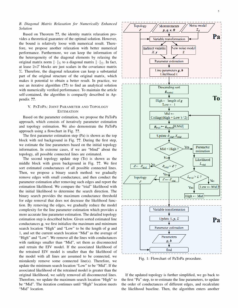
Based on the parameter estimation, we propose the PaToPaapproach, which consists of iteratively parameter estimationand topology estimation. We also demonstrate the PaToPaapproach using a flowchart in Fig. ??.

The first parameter estimation step (Pa) is shown as the topblock with red background in Fig. ??. During the first step,we estimate the line parameters based on the initial topologyinformation. In extreme cases, if we are “blind” about thetopology, all possible connected lines are estimated.

The second topology update step (To) is shown as themiddle block with green background in Fig. ??. We firstsort estimated conductances of all possible connected lines.Then, we propose a binary search method: we graduallyremove edges with small conductance, and then conduct theparameter estimation after removing such edges and report theestimation likelihood. We compare the “trial” likelihood withthe initial likelihood to determine the search direction. Thebinary search provides the maximum conductance thresholdfor edge removal that does not decrease the likelihood func-tion. By removing the edges, we gradually reduce the modelcomplexity for the line parameter estimation which provides amore accurate line parameter estimation. The detailed topologyestimation step is described below. Given sorted estimated lineconductances g, we first initialize the maximum and minimumsearch location “High” and “Low” to be the length of g and1, and set the current search location “Mid” as the average of“High” and “Low”. We remove all the lines with conductanceswith rankings smaller than “Mid”, set them as disconnectedand retrain the EIV model. If the associated likelihood ofthe retrained EIV model is smaller than the likelihood ofthe model with all lines are assumed to be connected, wemistakenly remove some connected line(s). Therefore, weupdate the minimum search location “Low” to be “Mid”. If theassociated likelihood of the retrained model is greater than theoriginal likelihood, we safely removed all disconnected lines.Therefore, we update the maximum search location “High” tobe “Mid”. The iteration continues until “High” location meets“Mid” location.

Measurements

p, q, v, !

Variable transformation

Topology

!

Noise model

"0

Indirect variable

X, y

New noise model

"

Parameter estimation

Descending sort

gsorted

High ← length of g

Low ← 1

Mid ←

Ceiling((High + Low ) / 2)

gtrial ← gsorted[0:Mid]

Update !trial, Xtrial

Mid < High ?

! ← !trial !trial = ! ?

! ← !trial

Topology

!

Line parameters g, b

Likelihood L

Yes

No

Yes

No

Parameter

estimation

Likelihood

Ltrial

Ltrial > L ?

Low ← Mid

High ← Mid

No

Yes

Pa

Parameters

g, b

Parameter estimation

Variable transformation

Update X, y, "

End

Pa

To

Fig. 1: Flowchart of PaToPa procedure.

If the updated topology is further simplified, we go back tothe first “Pa” step, to re-estimate the line parameters, to updatethe order of conductances of different edges, and recalculatethe likelihood baseline. Then, the algorithm enters another

6

round of topology update.If the updated topology is the same as the original topology,

we know the topology cannot be further simplified. Then, weuse the final topology estimation result to conduct anotherparameter estimation (Pa) to generate the final output. Thefinal parameter update step is shown as the bottom block withblue background in Fig. ??.

The algorithm for the proposed PaToPa training flow alsois shown in Algorithm ??. The “UpdateTopo” function in line

Algorithm 1 Parameter and Topology Joint Estimation

1: procedure PATOPA(P,Q, V,Θ,Σ0)2: y ← GENY(P,Q, E)3: X ← GENX(V,Θ, E)4: Σ← GENVAR(Σ0, E)5: E ′ ← Kn6: E ← ∅7: while E 6= E ′ do8: E ← E ′9: X,y,Σ← UPDATEDATA(X,y,Σ, E)

10: g, b← EIV(X,y,Σ)11: i← TOPOEST(X,y, g, b,Σ)12: E ′ ← UPDATETOPO(E , g, i)13: end while14: return E , g, b15: end procedure

12 is just removing the edges based on the threshold i andthe sorted conductance g. The topology estimation algorithm“TopoEst”, which is the key module in Algorithm ??, is shownin Algorithm ?? and is extensively discussed below. Theo-

Algorithm 2 Topology Update

1: procedure TOPOEST(X,y, g, b,Σ)2: l = LIKELIHOOD(X,y, g, b,Σ)3: m← length of g4: n← length of y5: imin, imax = 0,m− 16: while imax > imin + 1 do7: i← imax+imin

28: s← {j} ⊆ {0, · · · ,m− 1} if g[j] ≥ g[i]9: X ← [X[0 : 2n/3, s], X[0 : 2n/3, s+m]]

10: y ← y[0 : 2n/3]11: Xv ← [X[2n/3 : n− 1, s], X[2n/3 : n− 1, s+m]]12: yv ← y[2n/3 : n− 1]13: g, b← EIV(X, y)14: l← LIKELIHOOD(Xv, yv, g, b,Σ)15: if l > l − 0.2|l| then16: imin ← i17: else18: imax ← i19: end if20: end while21: return imin

22: end procedure

rem ?? demonstrates that Algorithm ?? will not mistakenlyremove a connected branch.

Theorem 2. When we set a connected edge to be discon-nected, the log-likelihood of the best fit must be smaller thanthe connected situation when measurement error is small.

Proof. The optimization problem (??) maximizes the log-likelihood

−∥∥∥[X,y]−

[X, y

]∥∥∥2

Σ, (29)

where X and y are measurements. By denoting X = X0+δX ,y = y0+δy, where X0 and y0 are the noiseless values and δXand δy are the measurement noises, we can write the optimallog-likelihood l as a function of the measurement noise δXand δy:

l (δX, δy) . (30)

For noiseless X0 and y0, there exists true line parameters asuch that y0 = X0a, hence the optimal solution of (??) is justX = X0, y = y0, and the optimal log-likelihood l(0, 0) = 0.

We first prove that, if X0, the noiseless value of historicaldata, is full rank, there does not exist a b with the samedimension as a satisfying y0 = XT

0 b if for some i, bi = 0,ai 6= 0. We prove it by contradiction: if there exists sucha b, we have the following: y0 = X0a = X0b. Hence,X0(a − b) = 0. However, since X0 is full rank, the equalityholds only a− b = 0 [?], which contradicts to ai − bi 6= 0.

Actually, if we remove the ith column of X0 and δX in theoptimization problem (??), we can get the optimal solution ofb and the associated log-likelihood:

l2(δX−i, δy), (31)

where δX−i represents the new matrix from removing the ithcolumn of δX . The noiseless case simply says l(0, 0) = 0 >l2(0, 0). The difference is merely determined by the underlyingtrue values X0 and y0. We denote the difference as

τ = l(0, 0)− l2(0, 0). (32)

From [?], the functions l(·) and l2(·) are both continuouseven if the optimization problem is non-convex. Therefore,for any τ > 0, there exists an ε > 0, such that forany δX, δX−i, δy satisfying ‖δX‖F < ε, ‖δX−i‖F < ε,‖δy‖ < ε, we have

‖l (0, 0)− l (δX, δy) ‖ < τ

3, (33)

and‖l2 (0, 0)− l2 (δX−i, δy) ‖ < τ

3. (34)

Therefore, for small enough measurement errors, the loglikelihood of the connected situation is greater than the loglikelihood of the case that a connected edge is assumed to bedisconnected:

l (δX, δy) > l2 (δX−i, δy) . (35)

In Algorithm ??, we use a separate validation set to esti-mate the likelihood to ensure the efficiency, and set a looserlikelihood update criteria: l > l − 0.2‖l‖ of the topologyupdates. In practice, if the measurement error is small enough,removing a connected line in the system model will result in

7

likelihood decrease in order of magnitudes. Therefore, settingup an l − 0.2‖l‖ threshold helps the iteration move forwardwithout introducing errors.

A. Recover Admittance Matrix from Joint Topology and LineParameter Estimation

After we obtain the estimated topology E and the associatedline parameters g, b, we can easily recover the admittancematrix Y with the help of the incidence matrix S and theindexing matrix U introduced in Section ??.

Remark 2. The proposed PaToPa framework works with meshnetworks, in addition to radial networks, since it treats edgesequally without using any radial network properties.

B. Recover Equivalent Admittance Matrix when There arePartial Measurements

In many distribution grids, the measurements are only avail-able at the root level where the substation/feeder transformersare located, and the leaf level where the residential loads anddistributed energy resources are located. In the intermediatelevel buses, no measurements are available. When there areno power injections in hidden buses, the distribution gridcould be treated as an equivalent network with only theroot node and leaf nodes due to the Kron reduction of theadmittance matrix. In detail, for such a network, we canintroduce an equivalent admittance matrix which representsa connected graph among active buses which have non-zeropower injections. For this case, the proposed PaToPa approachcan still learn the equivalent topology and line parameters forthe reduced equivalent network and could be used for furtheranalysis, such as state estimation and power flow analysis.

C. Parameter Estimation without Strict PMU Requirement

When the number of available PMU measurements is re-duced, we need to evaluate the impact and see if (??) is stillcomputable. Due the flexibility of our input error modeling,we can accommodate one or more buses without PMUs withacceptable information loss for parameter estimation. Theunknown phase angle could be effectively treated as anothersource of input noises and the measurement error is the anglebetween zero and the actual value. Since this modification onlychange the observed phase angle, all the following derivation,including the first order Taylor’s expansion could be done inthe same manner.

Since the phase angle differences across buses in distri-bution grids are much smaller than the phase angle dif-ferences in transmission grids, a small error will be intro-duced when we treat the phase angles as zero. For ex-ample, if PMU measurement θui1 is unavailable, it intro-duces error into cij , but cij is still computable via cij =|sji|

(v2i − vuj1vuj2 cos

(sji(0− θuj2

))), so X in (??) is still

computable. After computing the X , the associated covariancematrix Σ could be derived from the first order Taylor’sexpansion (??) at a new position φ, where θuj1 = 0.

In summary, the proposed PaToPa framework is very robustagainst system complexity and measurements constraints.

VI. EXPERIMENTAL RESULTS

A. Numerical Setup

We test our joint topology and line parameter estimationapproach on a variety of settings and real-world data sets. Forexample, we use IEEE 8, 16, 32, 64, 96, 123-bus test feeders.The IEEE 16, 32, 64, 96-bus test feeders are extracted from theIEEE 123-bus system. The voltage and phase angle data arefrom two different feeder grids of Southern California Edison(SCE). The actual voltage and phase angle measurement datafrom SCE are used to generate the power injection data ateach bus on standard IEEE test grids. Gaussian measurementnoises are added to all measurements for the standard IEEEtest grids. The standard deviation of the added measurementerror is computed from the standard deviation of the historicaldata. For example, a 10% relative error standard deviationmeans that the standard deviation of the historical data ofsome measurement is 10 times the standard deviation of themeasurement error. The SCE data set’s period is from Jan.1, 2015, to Dec. 31, 2015. Simulation results are similar fordifferent test feeders. For illustration purpose, we use the 8-bussystem for performance demonstration.

B. Accuracy of Joint Parameter and Topology Estimation

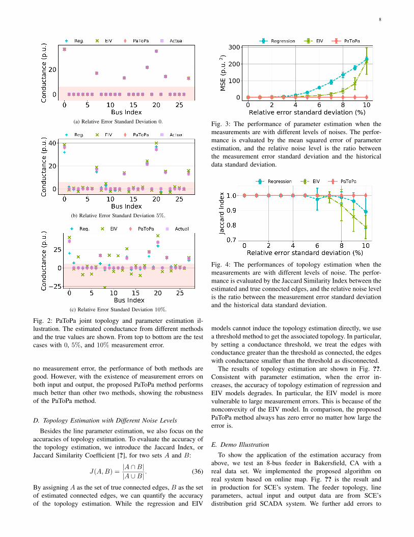
For an 8-bus system, there are 28 potential connections,represented in the x-axis of Fig. ??. Since the IEEE 8-busdistribution grid has a radial structure, there are 7 actual con-nections. For each potential connection, our joint topology andline parameter estimator will provide a parameter estimation,shown in the y-axis. As there is no noise in the setup thatgenerates Fig. ??, we observe a perfect match between theestimated line parameters g (red diamonds) and the underlyingtrue value g? (purple squares). In addition to the accurate lineparameter estimation, a simple threshold in light red shadescan detect the topology perfectly, leading to highly accuratejoint topology and line parameter estimation. When there arenoises in both input (θ, v) measurements and output (p, q)measurements, Fig. ?? and Fig. ?? illustrate the accuracy ofthe proposed PaToPa method. Even for 10% relative errorstandard deviation, when the regression model and EIV modelintroduce huge error, shown in Fig. ??, the propose PaToPamodel successfully captures these noises, leading to the perfecttopology identification and accurate line parameter estimation.

C. Parameter Estimation with Different Noise Levels

To summarize different testing results, we look into thestatistics in error domain. As shown in Fig. ??, when lineparameters are estimated accurately, the topology error issmall. Therefore, we focus on the statistical summary ofline parameter estimation in Fig. ??. For comparison, theperformance of the linear regression is plotted in blue, andthe performance of the EIV model is plotted in green. Foreach error level on the x-axis of Fig. ??, we test the threeapproaches on 30 different historical data sets with 500historical data points. The proposed PaToPa method alwayshas a smaller error than both the regression method and EIVmethod. The associated error bars indicate that when there is

8

(a) Relative Error Standard Deviation 0.

(b) Relative Error Standard Deviation 5%.

(c) Relative Error Standard Deviation 10%.

Fig. 2: PaToPa joint topology and parameter estimation il-lustration. The estimated conductance from different methodsand the true values are shown. From top to bottom are the testcases with 0, 5%, and 10% measurement error.

no measurement error, the performance of both methods aregood. However, with the existence of measurement errors onboth input and output, the proposed PaToPa method performsmuch better than other two methods, showing the robustnessof the PaToPa method.

D. Topology Estimation with Different Noise Levels

Besides the line parameter estimation, we also focus on theaccuracies of topology estimation. To evaluate the accuracy ofthe topology estimation, we introduce the Jaccard Index, orJaccard Similarity Coefficient [?], for two sets A and B:

J(A,B) =|A ∩B||A ∪B|

. (36)

By assigning A as the set of true connected edges, B as the setof estimated connected edges, we can quantify the accuracyof the topology estimation. While the regression and EIV

Fig. 3: The performance of parameter estimation when themeasurements are with different levels of noises. The perfor-mance is evaluated by the mean squared error of parameterestimation, and the relative noise level is the ratio betweenthe measurement error standard deviation and the historicaldata standard deviation.

Fig. 4: The performances of topology estimation when themeasurements are with different levels of noise. The perfor-mance is evaluated by the Jaccard Similarity Index between theestimated and true connected edges, and the relative noise levelis the ratio between the measurement error standard deviationand the historical data standard deviation.

models cannot induce the topology estimation directly, we usea threshold method to get the associated topology. In particular,by setting a conductance threshold, we treat the edges withconductance greater than the threshold as connected, the edgeswith conductance smaller than the threshold as disconnected.

The results of topology estimation are shown in Fig. ??.Consistent with parameter estimation, when the error in-creases, the accuracy of topology estimation of regression andEIV models degrades. In particular, the EIV model is morevulnerable to large measurement errors. This is because of thenonconvexity of the EIV model. In comparison, the proposedPaToPa method always has zero error no matter how large theerror is.

E. Demo Illustration

To show the application of the estimation accuracy fromabove, we test an 8-bus feeder in Bakersfield, CA with areal data set. We implemented the proposed algorithm onreal system based on online map. Fig. ?? is the result andin production for SCE’s system. The feeder topology, lineparameters, actual input and output data are from SCE’sdistribution grid SCADA system. We further add errors to

9

Fig. 5: Joint estimation for an 8-bus feeder in Bakersfield,CA. The relative standard deviation of measurement error is5%., and the topology and parameters are estimated through600 historical data points. For clearness, the online dashboardonly shows the estimated conductance.

all measurement variables. Fig. ?? shows a real-time onlinedashboard with our integrated algorithm running in the backend. The left panel shows the actual topology and the lineconductances in orange. The right panel shows the estimatedtopology and line parameters in blue. Fig. ?? shows that thetopology is reconstructed with 0% error, and the estimated lineparameters have a relative error of merely 1%.

F. The Choice of Matrix Relaxation Methods For PaToPaWe also systematically examine the two matrix relaxation

methods in the proposed PaToPa workflow. In particular, wecompare the log likelihood of the identity matrix relaxationwith the log likelihoods of the diagonal matrix relaxationduring different iterations in computing the results of thegeneralized total least square problem. Fig. ?? shows thelog likelihood of the diagonal matrix relaxation approachfor different iterations. We also plot the log likelihood ofthe identity matrix relaxation approach as a horizontal line.After only two iterations, the log likelihood of the diagonalmatrix relaxation becomes greater than the log likelihood ofthe identity matrix relaxation.

However, we also need to check whether the equality con-straint, or the equivalent norm deficiency constraint is satisfied,during the iterations. The results are shown in Fig. ??. Noticethat the identity matrix relaxation provides the guaranteeof the satisfaction of the norm deficiency constraint, whichshould result infinite condition number. Due to limited digitsin numerical calculation, the condition number for diagonalmatrix relaxation solution is on the scale of 1015. As wecan see, the condition number for diagonal matrix relaxationincreases slowly. The condition number achieve the scale of1015 after 100 iterations.

Fig. ?? and Fig. ?? validates the performance of thediagonal matrix relaxation. Furthermore, we illustrate that therequirement of the number of iterations mainly comes fromthe constraints, rather than the objective function.

G. Computing TimeIn the proposed PaToPa algorithm, the convergence of both

inner binary search and outer iteration is very fast, since

Fig. 6: The improvement of log-likelihood over iterations.While the identify matrix relaxation results an analyticalsolution the diagonal matrix relaxation requires the numericaliteration. After 2-3 iterations, the log-likelihood of the Diago-nal Matrix Relaxation becomes larger than the log likelihoodof the identity matrix relaxation.

0 25 50 75 100 125Number of Iterations

10410810121016

Cond

ition

Num

ber

Identity Matrix RelaxationDiagonal Matrix Relaxation

Fig. 7: The improvement of the condition number over itera-tions. Only after 100 iterations, the condition number of theoptimal solution’s matrix with diagonal matrix relaxation isgreater than the condition number of the optimal solution’smatrix with identity matrix relaxation.

the complexity of both is at the order of logarithm of thenumber of the possible branches. Therefore, the major factoraffecting computing time is the size of training dataset, sincethe matrix size which needs singular value decompositionis proportional to the size of training dataset. We evaluatethe computing time for an 8-bus system with 28 possiblebranches, for training set size from 100 to 500, shown inFig. ?? We use a single 2.6GHz Intel Core i5 CPU and 4 GBmemory for the evaluation. The singular value decompositionis computed by using standard numpy’s linalg.svd method. Fortraining set with length 500, the time cost for proposed PaToPaalgorithm is around 10 seconds. The EIV algorithm also needsperforming singular value decomposition, therefore, the timeconsumption is comparable to PaToPa approach. In contrast,the linear regression only requires matrix inverse. Therefore,the time consumption is less than 0.1 second for 500 trainingsamples. We can further improve the time complexity byimplementing parallel computing and using more specificsingular value decomposition algorithm designated for sparsematrix.

10

100 150 200 250 300 350 400 450 500Number of training points

10−210−1100101

Time co

st (s

)Regression EIV PaToPa

Fig. 8: Time complexity evaluation.

VII. CONCLUSION

Detailed system information such as grid topology and lineparameters are frequently unavailable or missing in distribu-tion grids. This prevents the required monitoring and controlcapability for deep DER integration. We propose to extendthe existing sensor capability (smart meters, µPMUs, andinverter sensors) by using their measurement data for jointtopology and line parameters estimation in distribution grids.Different from other methods which only consider outputmeasurement error and assume the topology is already known,our method correctly address the input-output measurementerror model with out topology requirement. By using theinteraction between input-output noises and nonlinear powerflow equations in parameter estimation,, we build an error-in-variables model in an MLE problem for joint topology and lineparameter estimation. With variable transformation and noisesdecorrelation, we successfully convert the NP-hard problemto a generalized low-rank approximation problem with aclosed form solution. Notably, our proposed approach doesnot require line measurements, making it robust in distributiongrids with a high topology uncertainty. Numerical results onIEEE test cases and real datasets from South California Edisonshow the superior performance of our proposed method.

APPENDIX ALEAST SQUARES AND TOTAL LEAST SQUARES

A. Maximum Likelihood Estimation (MLE) for TraditionalRegressions

Traditionally, the parameter estimation model only includesthe measurement error in the output. We generalize the powerflow equation as a mapping f(·; g, b) : Rn → R from the statex to the dependent variable y. If both the measurements of xand y are noiseless, we have

y = f(x; g, b). (37)

If the measurement noise solely comes from the dependentvariable y, the relationship between the measurements yt andthe state xt at time t is

yt − εyt = y?t = f(xt; g, b). (38)

We usually assume that εyt is independent of time stamp t andthe measurement yt and is sampled from i.i.d. random vari-ables. Under this assumption, given a series of measurementsy = [y1, · · · , yT ] and X = [x1, · · · ,xT ], we can formulate a

Maximum Likelihood Estimation (MLE) problem to find theoptimal estimate of the model parameter a:

g?, b? = arg maxg,b

logP (y|X, g, b). (39)

We can further write the MLE in a more detailed manner:

maxy,g,b

logP (y|y), (40a)

subject to yt = f(xt; g, b). (40b)

Furthermore, if the errors are i.i.d. Gaussian random vari-ables, the log likelihood function is a simple sum of squarefunctions. In addition, if the function f is a linear functionwith respect to [g; b], (??) becomes

miny,g,b

T∑t=1

(yt − yt)2, (41a)

subject to yt = [g; b]Txt. (41b)

The solution to such an MLE problem (??) has a closed-form(Least-Squares) solution:

(g?LS, b?LS) := (XTX)−1XTy. (42)

B. Error-In-Variables: Maximum Likelihood Estimation withMeasurement Errors on All Variables

However, the assumption that the measurement error onlycomes from the dependent variable y is incomplete. In ourcase, both power injections p, q and voltage phasors v,θ aremeasurements. Therefore, the noises on all measurements areunavoidable, e.g., the PMUs’ calibration error. Therefore, themapping relationship (??) turns into:

yt − εyt = f(xt − εxt ; g, b). (43)

Therefore, the MLE problem becomes:

maxX,y,g,b

logP (X,y|X, y), (44a)

subject to yt = f(xt; g, b). (44b)

The difficulty of solving (??) comes from the nonlinearityof (??).

However, when the measurement noise is i.i.d. Gaussiandistributed, and the mapping f is linear, a mature techniquecalled low-rank approximation can be used [?]. In particular,the log of the probability density function for i.i.d. Gaussianvariables is the sum of the measurement error squares. In thiscase, the optimization problem (??) turns into

minX,y,g,b

T∑t=1

‖xt − xt‖2 + (yt − yt)2, (45a)

subject to yt = (g, b)T xt. (45b)

Maximizing the log likelihood is equivalent to minimizingthe sum of the element-wise squares of the matrix [X,y] −[X, y], which is the Frobenius norm. In addition to objectivetransformation, the constraint could be transformed from y =[gT , bT ]x to [X, y][g; b;−1] = 0, meaning [X, y] is rankdeficient and [g; b;−1] lies in the null space.

11

Therefore, we can reformulate the parameter estimationproblem with measurement errors in both input and outputas a low-rank approximation problem for a linear system as:

minX,y‖[X,y]− [X, y]‖2F , (46a)

subject to Rank([X, y]) < n+ 1. (46b)

If the sample matrix [X,y] is full rank, (??) has a closedform solution, called Total Least Square (TLS) ?? [?], [?]:

[g?TLS; b?TLS] = (XTX − σ2T+1I)−1XTy, (47)

where σT+1 is the smallest singular value of the expandedsample matrix [X,y]. However, f is nonlinear for powersystems and the resulting MLE problem (??) is usually NP-hard at a first look.

APPENDIX BTHE APPROXIMATE BEHAVIOR OF THE TRUNCATED

NORMAL DISTRIBUTION AND THE ASSOCIATED MLEPROBLEM

In Section ??, we first use the first-order approximationof the induced measurement error, and then assume that theinduced error random variable is normal. In this section, weprovide a explanation of the detailed approximation procedure.We revisit the relationship between the original measurementerror εφ and the induced measurement error εc:

εc = h(εφ

). (48)

For clearer visualization, without introducing confusions, weremove the subscription i, j for c and h, and the parameter φof the function h compared with the main content.

We first assume that the distribution of the direct measure-ments εφ are sampled truncated normal distribution, truncatedat −d, d from normal distribution mean 0, standard deviationσ. If we denote the random variable of the truncated normaldistribution as Z(d;σ), the cumulative distribution function ofZ(d;σ) is:

F (x;σ, d) =Φ(xσ

)− Φ

(−dσ

)Φ(dσ

)− Φ

(−dσ

) , (49)

where Φ(·) is the cumulative distribution function of standardnormal distribution.

Theorem 3. The truncated normal distribution random vari-able Z(d;σ) converges to the normal distribution with meanzero, standard deviation σ in distribution when d→∞:

limd→∞

Z(d;σ)D−→ N (0, σ) . (50)

Proof. Since

limd→∞

Φ

(d

σ

)= 1, (51a)

limd→∞

Φ

(−dσ

)= 0, (51b)

we havelimd→∞

F (x;σ, d) = Φ(xd

). (52)

Furthermore, the Taylor’s theorem says that

εc = h(0) + ∇h(τ )|τ=0 εφ+1

2εTφ Hf(τ )

∣∣τ=ηεφ

εφ, (53)

where 0 ≤ η ≤ 1, and Hf is the Hessian of the function f .By introducing this expression, we do not need to considerhigher order terms in Taylor’s expansion. If εφ is a truncateddistribution and the truncation range is small enough and thegradient ∇h(τ ) is non-zero when τ = 0, the second orderterm is a higher order error compared with the first orderterm. Therefore, by introducing the two-step approximation:Truncated normal distribution and Taylor’s expansion, we canuse the first-order approximation to express the induced mea-surement error as a linear function of the direct measurementerror.

APPENDIX CDIAGONAL MATRIX RELAXATION FOR GENERALIZED LOW

RANK APPROXIMATION PROBLEM

If we replace the covariance matrix Σ in (??) by a diagonalmatrix Σ, and denote [X,y] − [X, y] = A, [X, y] = A, theobjective function could be written as

∑i

∑j wij(aij−aij)2,

where Σ = diag({wij}). Furthermore, the low-rank constraintcould be interpreted as Ac = 0 for some nonzero c. Therefore,the optimization problem for diagonal matrix relaxation couldbe expressed as:

minA,c

∑i

∑j

wij(aij − aij)2 (54a)

Subject to: Ac = 0, cT c = 1. (54b)

Then, the Lagrangian of the optimization problem (??) is:

L(A, c, l, λ

)=

1

2

∑i

∑j

wij(aij − aij)2 + lT Ac+1

2λ(cT c− 1

)=0.

(55)

By setting the derivatives to zero, we have:

wij(aij − aij) = −licj , (56a)

AT l = cλ, (56b)

Ac = 0, (56c)

cT c = 1. (56d)

We further have λ = 0, since cT AT l = λ = 0. Without lossof generality, we consider that for all i, j, wij > 0. Thenwe define V as the reciprocal matrix of W : vij = 1/vij .We further introduce d = l/‖l‖, σ = ‖l‖. After definingthese, (??) becomes:

A = A− σdiag (d)V diag (c) , (57a)

ATd = 0, (57b)

Ac = 0, (57c)

cT c = 1, (57d)

dTd = 1. (57e)

12

By substituting (??) to (??), we get:

ATd = σdiag (c)V Tdiag (d)d. (58)

By substituting (??) to (??), we get:

Ac = σdiag (d)V diag (c) c. (59)

Then we can define two diagonal matrices:

Dd = diag(V Tdiag (d)d

),

Dc = diag (V diag (c) c) .(60)

After these preparation, the generalized low-rank approxima-tion problem is converted to:

Ac = σDcd, (61a)

ATd = σDdc, (61b)

cT c = 1, (61c)

dTd = 1. (61d)

An iterative method is proposed to solve (??). We firstimplement the QR decomposition for A:

A = [Q1, Q2]

[R0

]. (62)

With the QR decomposition, we can represent d and l by twonew variable z and w:

l = σd = Q1z +Q2w. (63)

Since Dcd ∈ R(A) from (??), we have QT2 Dcd = 0.Therefore, we get the update rule for w from z:

σQT2 Dcd = 0 = QT2 DcQ1z +QT2 DcQ2w

⇒w[k] = −(QT2 D

[k−1]c Q2

)−1 (QT2 D

[k−1]c Q1

)z[k].

(64)

Then we can update l from the definition:

l[k] = Q1z[k] +Q2w

[k], (65a)

x[k] =l[k]∥∥∥l[k]∥∥∥ . (65b)

From (??) we get the update rule for c and σ:

c[k] =R−TQ−1

1 D[k−1]c d[k]∥∥∥R−TQ−1

1 D[k−1]c d[k]

∥∥∥ , (66a)

σ[k] =

∥∥c[k]∥∥∥∥∥R−TQ−1

1 D[k−1]c d[k]

∥∥∥ . (66b)

Then we can compute D[k]d and D[k]

c from d[k] and c[k]. Thealgorithm is shown in Algorithm ?? [?]:

ACKNOWLEDGMENT

The authors thank SLAC National Accelerator Laboratoryand South California Edison for their supports.

Algorithm 3 GLRA for Diagonal Matrix Relaxation

1: procedure PARAMEST(A, Σ)2: W ← matrix

(diag(Σ)

)3: V ← reciprocal (W )4: Initialize c, d5: while Not Converging do6: Dd ← GETDD(d, V )7: Dc ← GETDC(c, V )8: z ← R−TDdc

9: w ← −(QT2 D

[k]c Q2

)−1 (QT2 D

[k]c Q1

)z

10: d← Q1z +Q2w

11: d← d‖d‖

12: c← R−TQ−11 Dcd

13: σ ← 1‖c‖

14: c← σc15: end while16: A← A− σdTV c17: return A18: end procedure

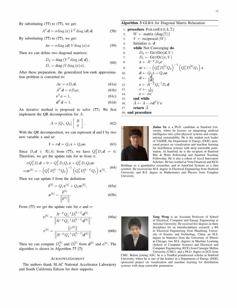
Jiafan Yu is a Ph.D. candidate at Stanford Uni-versity, where he focuses on integrating artificialintelligence into cyber-physical systems and compu-tational sustainability. He is the student tech leaderof VADER, the Department of Energy (DOE) spon-sored project on visualization and machine learningfor distribution systems with deep renewable pene-tration. At Stanford, he is the recipient of StanfordBits & Watts Fellowship and Stanford TeachingFellowship. He is also a cohort of Accel InnovationScholars. He has worked at Virtu Financial and KCG

Holdings as a quantitative researcher, and at AutoGrid Systems as a datascientist. He received his M.S. degree in Electrical Engineering from StanfordUniversity, and B.S. degree in Mathematics and Physics from TsinghuaUniversity.

Yang Weng is an Assistant Professor of Schoolof Electrical, Computer and Energy Engineering atArizona University. He received five degrees in threedisciplines for an interdisciplinary research: a BSin Electrical Engineering from Huazhong Univer-sity of Science and Technology, China, an M.S.degree in Statistics from the University of Illinoisat Chicago, two M.S. degrees in Machine Learning(School of Computer Science) and Electrical andComputer Engineering (ECE) from Carnegie MellonUniversity (CMU), and a Ph.D. degree in ECE from

CMU. Before joining ASU, he is a TomKat postdoctoral scholar at StanfordUniversity, where he is one of the leaders in a Department of Energy (DOE)sponsored project on visualization and machine learning for distributionsystems with deep renewable penetration.

13

Ram Rajagopal is an Associate Professor of Civiland Environmental Engineering and Electrical Engi-neering (by Courtesy) at Stanford University, wherehe directs the Stanford Sustainable Systems Lab(S3L), focused on large scale monitoring, data an-alytics and stochastic control for infrastructure net-works, in particular power and transportation. Hiscurrent research interests in power systems are inintegration of renewables, smart distribution systemsand demand-side data analytics. He has also builtwireless sensing systems and large-scale analytics

for transportation and power networks. He holds a Ph.D. in ElectricalEngineering and Computer Sciences and an M.A. in Statistics, both from theUniversity of California Berkeley. He is a recipient of the Powell FoundationFellowship, Berkeley Regents Fellowship, the NSF CAREER Award, theMakhoul Conjecture Challenge award and best paper awards in variousconferences. He holds more than 30 patents from his work, and has advisedor founded various companies in the fields of sensor networks, power systemsand data analytics.