pass-through in retail and wholesale - columbia …en2198/papers/retail_wholesale.pdfvol. 98 no. 2...

American Economic Review: Papers & Proceedings 2008, 98:2, 430-437

http://www. aeaweb. org/articles.php ?doi=10.1257/aer. 98.2.430

Pass-Through in Retail and Wholesale

By Emi Nakamura*

International economists have long studied retail prices to investigate the central question of how prices respond to exchange rates (e.g., Charles Engel 1993). Retail price data have also

played a key role in assessing empirical models of pricing in industrial organization and empirical macroeconomics. Yet, theoretical pricing models in these literatures have traditionally focused on

manufacturer behavior. Recent empirical work

suggests important differences in price dynam? ics at the retail versus the wholesale level of

production (Pinelopi K. Goldberg and Rebecca Hellerstein 2007; Nakamura 2007; Nakamura and Jon Steinsson 2007). This evidence suggests that

understanding the link between retail and whole? sale prices is key to developing pricing models that can fit the retail price data.1

This paper studies how prices co-move across

products, firms, and locations to gauge the rela? tive importance of retailer versus manufacturer level shocks in determining prices. I make use of a large panel dataset on prices for a cross section of retailers in the United States. I ana?

lyze prices at the barcode, or Universal Product Code (UPC), level for individual stores. I find that only 16 percent of the variation in prices is common across stores selling an identical

product. Sixty-five percent of the price variation is common to stores within a particular retail chain (but not across retail chains), while 17 per

cent is completely idiosyncratic to the store and

product.2 Product categories with frequent tem?

porary "sales" exhibit a disproportionate amount of completely idiosyncratic price variation.

My results suggest that most of the observed

price variation arises from retail-level rather than manufacturer-level demand and supply shocks. However, the behavior of prices is dif? ficult to reconcile with a model in which desired

prices move due to contemporaneous demand and supply shocks, a common set-up in mac?

roeconomics, international economics and industrial organization. This suggests that retail

prices may vary largely as a consequence of

dynamic pricing strategies on the part of retail? ers or manufacturers.3

The analysis I present here regarding the impor? tance of price variation at the level of individual retail stores is related to recent work in macroeco? nomics showing that large "idiosyncratic shocks" are needed to explain retail price fluctuations

(Golosov and Lucas 2007; Peter J. Klenow and

Oleksiy Kryvtsov 2007). In these models, the

"idiosyncratic shocks" driving price dynamics are shocks to manufacturers' productivity. Such

productivity shocks would, however, generate substantial co-movement across prices for the same good at different retail stores. I show that we observe little such co-movement. My results

suggest that we must delve deeper for the source of the large observed fluctuations in retail prices.

I. Data

This paper uses a new dataset on prices from AC Nielsen. The novel feature of the dataset is

* Columbia Business School and Department of Eco?

nomics, Columbia University, 3022 Broadway, New York, NY 10027, and National Bureau of Economic Research

(e-mail: [email protected]). I would like to thank

David Bell, Charles Engel, Tim Erickson, Penny Goldberg, Rebecca Hellerstein, David Hosken, Rob McClelland, John

Greenlees, Ephraim Leibtag, Alice Nakamura, Aviv Nevo, Ariel Pakes, and J?n Steinsson for many useful conversa?

tions related to this project. I would like to thank the US

Department of Agriculture, Economic Research Service

(USDA ERS) for financial support for this project. 1 This work is also closely related to recent papers in

international economics attempting to measure and study the theoretical implications of "distribution margins." See for example, Ariel T Burstein, Joao C. Neves, and Sergio Rebelo (2003).

2 Retailers are, of course, not necessarily the source

of price variation idiosyncratic to particular retail chains, since manufacturers may adjust their prices differently to

different retailers. I discuss this issue in Section III. 3 For example, see Hal R. Varian (1980), Joel Sobel

(1984), Victor Aguirregabiria (1999) and Edward P. Lazear

(1986) for models in which the firm's desired price varies

endogenously. Patrick Kehoe and Virgiliu Midrigan (2007) study an alternative model of sales, in which sales arise due to transitory demand and supply shocks.

430

This content downloaded from 128.59.160.114 on Tue, 16 Jun 2015 22:18:52 UTCAll use subject to JSTOR Terms and Conditions

http://www.jstor.org/page/info/about/policies/terms.jsp

VOL. 98 NO. 2 PASS-THROUGH IN RETAIL AND WHOLESALE 431

its large cross-sectional dimension. The data consist of price and quantity series for about

7,000 grocery stores across the United States. These grocery stores are members of 33 major chains and cover 50 major US cities. The time series coverage is short: the data cover all 12

months of 2004. The dataset includes approxi? mately 100 different UPCs selected within a wide variety of grocery store food categories.4 In total, the dataset consists of about 50 million observations.

Few papers have studied the co-movement of prices across retailers, perhaps because most

price data available to academic researchers cover only a narrow cross section of retailers.5 The most closely related work to the present analysis is Daniel Hosken and David Reiffen

(2004). They show that sales account for a large fraction of the variation in prices, and find sup? port for the view that these transitory price fluctuations reflect temporary changes in retail

margins rather than wholesale price changes.6 The huge cross-sectional dimension of my data

allows me to carry out a more detailed analysis of price variation across products, stores, and cities than has been possible using other data sources. In the case of the US Bureau of Labor Statistics (BLS) CPI Research Database data studied by Hosken and Reiffen (2004), on aver?

age seven price quotes are collected per month for each item category and area. In many cases, BLS price collectors collect different UPCs at different stores for the same product category, implying that often only a single observation is available for a unique UPC at a given point in time.7 Hosken and Reiffen (2004), therefore,

1 4 7 10 13 16 19 22 25 28 31 34 37 40 43 46 49 52 Week

Figure 1. Prices and Regular Prices

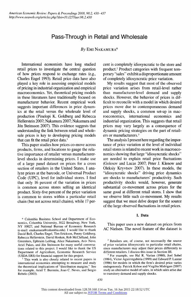
Notes: The figure plots a price series for a 12-pack of 12 ounce Diet Pepsi from a particular store in the dataset. The

regular price is constructed according to the "sale filter"

algorithm described in the text. The missing observations

correspond to weeks when no units were sold.

analyze the role of manufacturers by studying the comovement of prices within narrowly defined

product categories, rather than at the barcode

(UPC) level. My data also have a much greater number of price quotes for identical UPCs at a

given point in time than AC Nielsen "scanner

panel" data based on household surveys.8 It is important to note that the sample of stores

included in the present dataset is not randomly selected. First, not all stores agree to provide AC Nielsen with data, and to share this data in dis?

aggregated form. It is well known that Walmart does not share its data with AC Nielsen. Second, the data included in the dataset were selected to represent the largest US supermarket chains.

Supermarket chains accounting for a small frac? tion of retail sales, such as independent super? markets, are not included.

II. Results

I begin by documenting some basic properties of the price dynamics in the data. Figure 1 depicts

4 The categories are beer, bread, cereal, Cheddar cheese,

crackers, cream cheese, canned soup, coffee, flour, frank?

furters, ice cream, apple juice, margarine, marinara, oil, peanut butter, ravioli, lime diet soft drinks, cola, diet cola, lime soft drinks, other soft drinks, other diet soft drinks,

spaghetti, sugar, and tuna. In each product category, the data set includes the top 1-3 UPC's by national dollar sales value.

5 A substantial amount of academic research has

focused on the Dominick's Finer Foods database from the

University of Chicago Graduate School of Business, which covers a single retail chain.

6 In a related exercise, Ephraim Leibtag et al. (2007) study the synchronization of manufacturer price changes in the US coffee industry. They find substantial co-move?

ment in the timing of price changes across major coffee manufacturers.

7 See Christian Broda and David E. Weinstein (2007) for a discussion of the BLS sampling frame.

8 See, e.g., Broda and Weinstein (2007) for a discussion

of the AC Nielsen scanner panel data. While these data contain a huge number of observations, they reflect a much smaller cross section of prices for identical items, due to the modest size of the household panel, and the fact that consumers select from a huge array of different UPCs and often buy slightly different items.



432 AEA PAPERS AND PROCEEDINGS MAY 2008

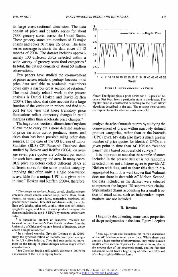
Table 1?Basic Statistics on Prices

Monthly frequency Price variability

All Regular All Regular Median 42.7% 17.5% 15.3% 9.1% Mean 43.9% 19.0% 15.3% 9.2% Sample size 43,006,064 43,006,064 43,006,064 43,006,064

Notes: The underlying data are weekly price observations. The "regular" price series is cal?

culated based on the filter described in the text. The monthly frequency of price change is

the fraction of the time that the weekly price (for a particular store and UPC) differs from the price four weeks earlier. Price variability is calculated by first logging and demeaning at

the store-UPC level and then calculating the standard deviation of this series. The statistics

above are means across product categories.

a typical series from the dataset, along with a

"regular" price series that excludes sales. Since there is no variable in the raw data indicating whether a product is on sale, I identify sales here and elsewhere in the paper using a crude "sale filter." The sale filter labels as a sale any price change that returns either to the original regular price or to a new (repeating) regular price.9

Columns 1 and 2 of Table 1 present summary statistics on the monthly frequency of price change for sale and nonsale price changes. The mean monthly frequency of price change across

categories is 42.7 percent, while the median is 43.9 percent. In most sectors, over half of price changes are associated with the temporary sales identified by the sale filter. The mean frequency of price change for regular prices across product categories is 17.5 percent, while the median is 19.0 percent.

Columns 3 and 4 of Table 1 present statis? tics on price variability. The statistic presented here is the standard deviation of prices for the

weekly price series. The underlying prices are first logged and demeaned by the average price for the store and UPC. The standard deviation, therefore, reflects time series variability of

prices in percentage terms. The table presents the mean and median of these statistics across

product categories. The time series variation in prices over the

course of a year is extremely large. The average standard deviation of log prices for the typical

product (relative to its mean) is about 15.3 per? cent. A comparison between the two columns reveals that a large fraction of the variance in

prices is accounted for by temporary sales. The mean standard deviation of regular prices is 9.2 percent, about two-thirds of the standard deviation including sales.10

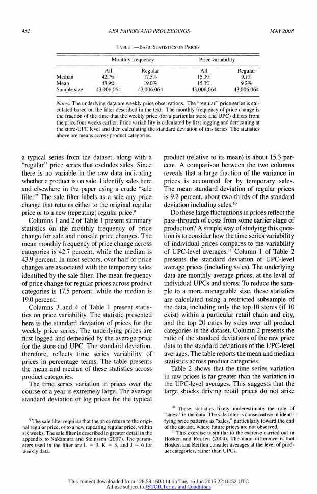
Do these large fluctuations in prices reflect the

pass-through of costs from some earlier stage of

production? A simple way of studying this ques? tion is to consider how the time series variability of individual prices compares to the variability of UPC-level averages.11 Column 1 of Table 2

presents the standard deviation of UPC-level

average prices (including sales). The underlying data are monthly average prices, at the level of individual UPCs and stores. To reduce the sam?

ple to a more manageable size, these statistics are calculated using a restricted subsample of the data, including only the top 10 stores (if 10

exist) within a particular retail chain and city, and the top 20 cities by sales over all product categories in the dataset. Column 2 presents the ratio of the standard deviations of the raw price data to the standard deviations of the UPC-level

averages. The table reports the mean and median statistics across product categories.

Table 2 shows that the time series variation in raw prices is far greater than the variation in the UPC-level averages. This suggests that the

large shocks driving retail prices do not arise

9 The sale filter requires that the price return to the origi? nal regular price, or to a new repeating regular price, within six weeks. The sale filter is described in greater detail in the

appendix to Nakamura and Steinsson (2007). The param? eters used in the filter are L = 3, K = 3, and J = 6 for

weekly data.

10 These statistics likely underestimate the role of "sales" in the data. The sale filter is conservative in identi?

fying price patterns as "sales," particularly toward the end of the dataset, where future prices are not observed.

11 This exercise is similar to the exercise carried out in Hosken and Reiffen (2004). The main difference is that Hosken and Reiffen consider averages at the level of prod? uct categories, rather than UPCs.




at the manufacturer level. Indeed, the common

UPC-level component is likely to be even less variable than is suggested by the analysis above, since some of the idiosyncratic store-level price

movements do not average out, even in this very large sample. In the next section, I consider a

more sophisticated procedure for decomposing the sources of variation in prices.

A. Variance Decompositions

I next consider a simple variance decompo? sition of prices (including sales). I decompose the variation in prices into two broad classes:

(a) price variation common to all items within a product category (e.g., beer) and (b) price variation idiosyncratic to particular UPCs.

Within each of these broad classes, I decompose the price variation into variation that is common across all stores, variation that is common only to stores within the same retail chain, and varia? tion that is completely idiosyncratic to particu? lar stores.12

I estimate the variance decomposition using panel data on prices, where each observation is the monthly average price for an individual UPC at an individual store (e.g., a 12-pack of 12-ounce Diet Pepsi at the Pathmark on 125th Street in New York City).13 These price observations are demeaned by the UPC and store-level mean so that all of the variability is time series variation. The subsample used in the estimation is the same one used to estimate the statistics in Table 2.

I estimate the variance decomposition sepa? rately for each product category and city in the dataset for which a sufficient amount of data are available.14 The categorization described above

implies six distinct sources of price variation

(three sources of variation each within of the

Table 2?Volatility of Prices versus UPC Average

Price variability

UPC Av. Ratio to Av.

Median 3.51% 2.7 Mean 4.28% 3.1 Sample size 1008 346,930

Notes: For each store and UPC, the raw weekly prices (including sales) are averaged within months, then logged and demeaned at the store-UPC level. The "UPC Av." is constructed by averaging this series across all retail stores. "Price Variability" is the standard deviation of this series. "Ratio to Av." is the ratio of price variability for the UPC store series to the price variability for the UPC Av. series. The statistics above are means across product categories.

two categories described above). These compo? nents are estimated using a standard maximum likelihood estimator.15

Table 3 reports the results of the variance

decomposition. Columns 1-3 report the fraction of price variation that is common within a prod? uct category. Column 1 reports the fraction that is common both across all UPCs within a prod? uct category and across all stores in the dataset. Column 2 reports the fraction of the variation that is common within the product category and across stores in a particular retail chain (but not across retail chains). Finally, column 3 reports the fraction of the variation that is common only to a product category and store (but not across

stores).

Columns 4-6 report a similar set of statis? tics for the components of price variation that are idiosyncratic to particular UPCs. Column 4

reports the fraction of UPC-level variation that is common across all stores within the same city. Column 5 reports the fraction of UPC-level vari? ation that is common within a particular retail chain (but not across retail chains). Finally, col? umn 6 reports the fraction of UPC-level varia? tion that is idiosyncratic to a particular store and

UPC. All statistics are calculated by first aver

12 I do not adjust the prices for inflation. CPI inflation was 2.9 percent between January 2004 and January 2005 and therefore has little effect on my results. Over longer time periods, it would be essential to consider a model

allowing for trend inflation. 13 I consider prices averaged over months because this

allows the variance decomposition to capture correla? tions between price changes at retailers in slightly differ? ent weeks, as long as the price changes occur in the same month. The results from the variance decomposition are

very similar if I use prices for the first week of each month rather than monthly average prices. 14

For the model to be identified, there must be at least two retail chains that sell products in the city/product cat?

egory, and at least two UPCs in the product category.

15 The variance decomposition is implemented using a

random effects model with i.i.d. shocks for each of the six

components. These estimates do not account for dynamic correlations, though I analyze monthly average prices to allow for correlations across weeks within a month.

Alternative approaches to estimating variance components models include ANOVA and REML. See, e.g., Baltagi (2005) for an excellent survey of these methods. See Table 3 for a listing of the variance components.




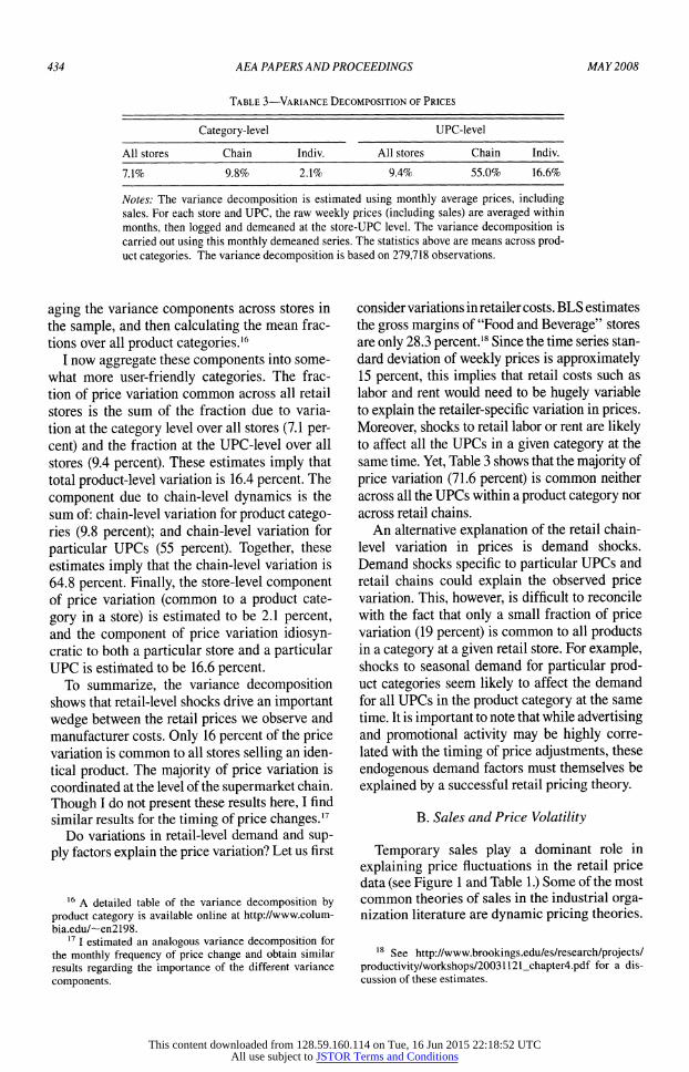
Table 3?Variance Decomposition of Prices

Category-level UPC-level

All stores Chain Indiv. All stores Chain Indiv.

7.1% 9.8% 2.1% 9.4% 55.0% 16.6%

Notes: The variance decomposition is estimated using monthly average prices, including sales. For each store and UPC, the raw weekly prices (including sales) are averaged within

months, then logged and demeaned at the store-UPC level. The variance decomposition is

carried out using this monthly demeaned series. The statistics above are means across prod? uct categories. The variance decomposition is based on 279,718 observations.

aging the variance components across stores in the sample, and then calculating the mean frac? tions over all product categories.16

I now aggregate these components into some?

what more user-friendly categories. The frac? tion of price variation common across all retail stores is the sum of the fraction due to varia? tion at the category level over all stores (7.1 per? cent) and the fraction at the UPC-level over all stores (9.4 percent). These estimates imply that total product-level variation is 16.4 percent. The

component due to chain-level dynamics is the sum of: chain-level variation for product catego? ries (9.8 percent); and chain-level variation for

particular UPCs (55 percent). Together, these

estimates imply that the chain-level variation is 64.8 percent. Finally, the store-level component of price variation (common to a product cate?

gory in a store) is estimated to be 2.1 percent, and the component of price variation idiosyn? cratic to both a particular store and a particular UPC is estimated to be 16.6 percent.

To summarize, the variance decomposition shows that retail-level shocks drive an important wedge between the retail prices we observe and

manufacturer costs. Only 16 percent of the price variation is common to all stores selling an iden? tical product. The majority of price variation is coordinated at the level of the supermarket chain.

Though I do not present these results here, I find similar results for the timing of price changes.17

Do variations in retail-level demand and sup?

ply factors explain the price variation? Let us first

consider variations in retailer costs. BLS estimates the gross margins of "Food and Beverage" stores are only 28.3 percent.18 Since the time series stan? dard deviation of weekly prices is approximately 15 percent, this implies that retail costs such as

labor and rent would need to be hugely variable to explain the retailer-specific variation in prices.

Moreover, shocks to retail labor or rent are likely to affect all the UPCs in a given category at the same time. Yet, Table 3 shows that the majority of

price variation (71.6 percent) is common neither across all the UPCs within a product category nor across retail chains.

An alternative explanation of the retail chain level variation in prices is demand shocks. Demand shocks specific to particular UPCs and retail chains could explain the observed price variation. This, however, is difficult to reconcile with the fact that only a small fraction of price variation (19 percent) is common to all products in a category at a given retail store. For example, shocks to seasonal demand for particular prod? uct categories seem likely to affect the demand for all UPCs in the product category at the same

time. It is important to note that while advertising and promotional activity may be highly corre?

lated with the timing of price adjustments, these

endogenous demand factors must themselves be

explained by a successful retail pricing theory.

B. Sales and Price Volatility

Temporary sales play a dominant role in

explaining price fluctuations in the retail price data (see Figure 1 and Table 1.) Some of the most common theories of sales in the industrial orga? nization literature are dynamic pricing theories.

16 A detailed table of the variance decomposition by

product category is available online at http://www.colum bia.edu/~en2198.

17 I estimated an analogous variance decomposition for

the monthly frequency of price change and obtain similar

results regarding the importance of the different variance

components.

18 See http://www.brookings.edu/es/research/projects/ productivity/workshops/20031121_chapter4.pdf for a dis?

cussion of these estimates.




Freq. Sales

?

? ? ?%

0 10 20 30 40 50 Frac. Residual Variance

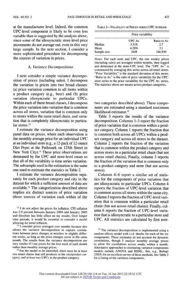
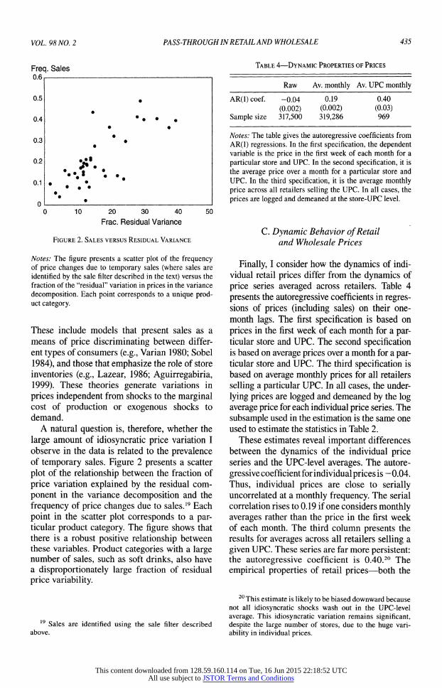
Figure 2. Sales versus Residual Variance

Notes: The figure presents a scatter plot of the frequency of price changes due to temporary sales (where sales are

identified by the sale filter described in the text) versus the fraction of the "residual" variation in prices in the variance

decomposition. Each point corresponds to a unique prod? uct category.

These include models that present sales as a means of price discriminating between differ? ent types of consumers (e.g., Var?an 1980; Sobel

1984), and those that emphasize the role of store inventories (e.g., Lazear, 1986; Aguirregabiria, 1999). These theories generate variations in

prices independent from shocks to the marginal cost of production or exogenous shocks to demand.

A natural question is, therefore, whether the

large amount of idiosyncratic price variation I observe in the data is related to the prevalence of temporary sales. Figure 2 presents a scatter

plot of the relationship between the fraction of

price variation explained by the residual com?

ponent in the variance decomposition and the

frequency of price changes due to sales.19 Each

point in the scatter plot corresponds to a par? ticular product category. The figure shows that there is a robust positive relationship between these variables. Product categories with a large number of sales, such as soft drinks, also have a disproportionately large fraction of residual

price variability.

0.5

0.4

0.3

0.2

0.1

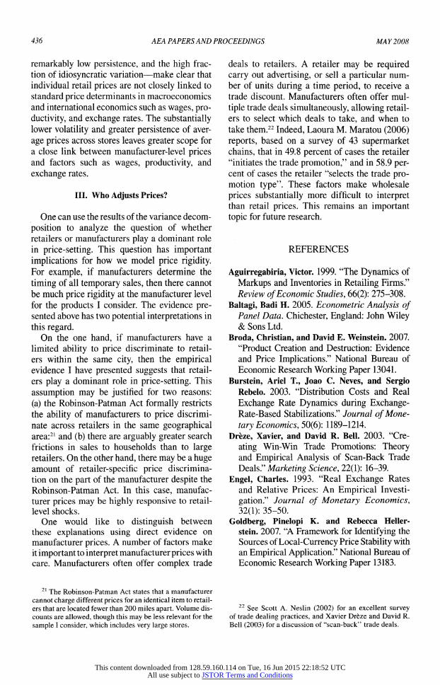
Table 4?Dynamic Properties of Prices

Raw Av. monthly Av. UPC monthly

AR(l)coef. -0.04 0.19 0.40

(0.002) (0.002) (0.03) Sample size 317,500 319,286 969

Notes: The table gives the autoregressive coefficients from

AR(1) regressions. In the first specification, the dependent variable is the price in the first week of each month for a

particular store and UPC. In the second specification, it is

the average price over a month for a particular store and

UPC. In the third specification, it is the average monthly

price across all retailers selling the UPC. In all cases, the

prices are logged and demeaned at the store-UPC level.

C. Dynamic Behavior of Retail and Wholesale Prices

Finally, I consider how the dynamics of indi? vidual retail prices differ from the dynamics of

price series averaged across retailers. Table 4

presents the autoregressive coefficients in regres? sions of prices (including sales) on their one

month lags. The first specification is based on

prices in the first week of each month for a par? ticular store and UPC. The second specification is based on average prices over a month for a par? ticular store and UPC. The third specification is based on average monthly prices for all retailers

selling a particular UPC. In all cases, the under?

lying prices are logged and demeaned by the log average price for each individual price series. The

subsample used in the estimation is the same one used to estimate the statistics in Table 2.

These estimates reveal important differences between the dynamics of the individual price series and the UPC-level averages. The autore?

gressive coefficient for individual prices is -

0.04. Thus, individual prices are close to serially uncorrelated at a monthly frequency. The serial correlation rises to 0.19 if one considers monthly averages rather than the price in the first week of each month. The third column presents the results for averages across all retailers selling a

given UPC. These series are far more persistent: the autoregressive coefficient is 0.40.20 The

empirical properties of retail prices?both the

19 Sales are identified using the sale filter described

above.

20 This estimate is likely to be biased downward because not all idiosyncratic shocks wash out in the UPC-level

average. This idiosyncratic variation remains significant, despite the large number of stores, due to the huge vari?

ability in individual prices.




remarkably low persistence, and the high frac? tion of idiosyncratic variation?make clear that individual retail prices are not closely linked to standard price determinants in macroeconomics and international economics such as wages, pro? ductivity, and exchange rates. The substantially lower volatility and greater persistence of aver?

age prices across stores leaves greater scope for a close link between manufacturer-level prices and factors such as wages, productivity, and

exchange rates.

III. Who Adjusts Prices?

One can use the results of the variance decom?

position to analyze the question of whether retailers or manufacturers play a dominant role in price-setting. This question has important implications for how we model price rigidity. For example, if manufacturers determine the

timing of all temporary sales, then there cannot be much price rigidity at the manufacturer level for the products I consider. The evidence pre? sented above has two potential interpretations in this regard.

On the one hand, if manufacturers have a limited ability to price discriminate to retail? ers within the same city, then the empirical evidence I have presented suggests that retail? ers play a dominant role in price-setting. This

assumption may be justified for two reasons:

(a) the Robinson-Patman Act formally restricts the ability of manufacturers to price discrimi? nate across retailers in the same geographical area:21 and (b) there are arguably greater search frictions in sales to households than to large retailers. On the other hand, there may be a huge amount of retailer-specific price discrimina? tion on the part of the manufacturer despite the

Robinson-Patman Act. In this case, manufac?

turer prices may be highly responsive to retail level shocks.

One would like to distinguish between these explanations using direct evidence on

manufacturer prices. A number of factors make it important to interpret manufacturer prices with care. Manufacturers often offer complex trade

deals to retailers. A retailer may be required carry out advertising, or sell a particular num? ber of units during a time period, to receive a trade discount. Manufacturers often offer mul?

tiple trade deals simultaneously, allowing retail? ers to select which deals to take, and when to take them.22 Indeed, Laoura M. Maratou (2006) reports, based on a survey of 43 supermarket chains, that in 49.8 percent of cases the retailer "initiates the trade promotion," and in 58.9 per? cent of cases the retailer "selects the trade pro? motion type". These factors make wholesale

prices substantially more difficult to interpret than retail prices. This remains an important topic for future research.

21 The Robinson-Patman Act states that a manufacturer cannot charge different prices for an identical item to retail? ers that are located fewer than 200 miles apart. Volume dis? counts are allowed, though this may be less relevant for the

sample I consider, which includes very large stores.

22 See Scott A. Neslin (2002) for an excellent survey of trade dealing practices, and Xavier Dr?ze and David R. Bell (2003) for a discussion of "scan-back" trade deals.

REFERENCES

Aguirregabiria, Victor. 1999. "The Dynamics of

Markups and Inventories in Retailing Firms." Review of Economic Studies, 66(2): 275-308.

Baltagi, Badi H. 2005. Econometric Analysis of Panel Data. Chichester, England: John Wiley & Sons Ltd.

Broda, Christian, and David E. Weinstein. 2007. "Product Creation and Destruction: Evidence and Price Implications." National Bureau of Economic Research Working Paper 13041.

Burstein, Ariel T., Joao C. Neves, and Sergio Rebelo. 2003. "Distribution Costs and Real

Exchange Rate Dynamics during Exchange Rate-Based Stabilizations." Journal of Mone?

tary Economics, 50(6): 1189-1214.

Dr?ze, Xavier, and David R. Bell. 2003. "Cre?

ating Win-Win Trade Promotions: Theory and Empirical Analysis of Scan-Back Trade Deals." Marketing Science, 22(1): 16-39.

Engel, Charles. 1993. "Real Exchange Rates and Relative Prices: An Empirical Investi?

gation." Journal of Monetary Economics,

32(1): 35-50.

Goldberg, Pinelopi K. and Rebecca Heller

stein. 2007. "A Framework for Identifying the Sources of Local-Currency Price Stability with an Empirical Application." National Bureau of Economic Research Working Paper 13183.




Golosov, M. and R. E. Lucas. 2007. "Menu Costs and Phillips Curves." Journal of Political Eco?

nomy, 115,171-99. Hosken, Daniel, and David Reiffen. 2004. "Pat?

terns of Retail Price Variation." RAND Jour? nal of Economics, 35(1): 128-46.

Kehoe, Patrick, and Virgiliu Midrigan. 2007. "Sales and the Real Effects of Monetary Pol?

icy." 2007. Federal Reserve Bank of Minne? sota Working Paper.

Klenow, Peter J., and Oleksiy Kryvtsov. 2007.

"State-Dependent or Time-Dependent Pricing: Does it Matter for Recent US Inflation?" http:// www.klenow.com/KK.pdf.

Lazear, Edward P. 1986. "Retail Pricing and Clearance Sales." American Economic Review, 76(1): 14-32.

Leibtag, Ephraim, Alice Nakamura, Emi Naka? mura, and Dawit Zerom. 2007. "Cost Pass

Through in the US Coffee Industry." United

States Department of Agriculture Economic Research Report 38.

Maratou, Laoura M. 2006. "Bargaining Power

Impact on Off-Invoice Trade Promotions in US Grocery Retailing." PhD diss. Cornell

University. Nakamura, Emi. 2007. "Accounting for Incom?

plete Pass-Through." http://www.columbia. edu/~en2198/papers/passthrough_dynamic. pdf.

Nakamura, Emi, and Jon Steinsson. 2007. "Five Facts about Prices: A R??valuation of Menu Cost Models." http://www.columbia.edu/ ~en2198/papers/fivefacts.pdf.

Neslin, S. A. 2002. "Sales Promotion." Marketing Science Institute, Cambridge, MA.

Sobel, Joel. 1984. "The Timing of Sales." Review

of Economic Studies, 51(3): 353-68.

Var?an, Hal R. 1980. "A Model of Sales." Ameri? can Economic Review, 70(4): 651-59.



pass-through in retail and wholesale - columbia …en2198/papers/retail_wholesale.pdfvol. 98 no. 2...

Documents