PART TWOPART TWO

cha1873X_p02.qxd 3/21/05 1:01 PM Page 104

ROOTS OF EQUATIONS

105

PT2.1 MOTIVATION

Years ago, you learned to use the quadratic formula

x = −b ± √b2 − 4ac

2a(PT2.1)

to solve

f(x) = ax2 + bx + c = 0 (PT2.2)

The values calculated with Eq. (PT2.1) are called the “roots” of Eq. (PT2.2). They repre-sent the values of x that make Eq. (PT2.2) equal to zero. Thus, we can define the root of anequation as the value of x that makes f(x) = 0. For this reason, roots are sometimes calledthe zeros of the equation.

Although the quadratic formula is handy for solving Eq. (PT2.2), there are many otherfunctions for which the root cannot be determined so easily. For these cases, the numericalmethods described in Chaps. 5, 6, and 7 provide efficient means to obtain the answer.

PT2.1.1 Noncomputer Methods for Determining Roots

Before the advent of digital computers, there were several ways to solve for roots of alge-braic and transcendental equations. For some cases, the roots could be obtained by directmethods, as was done with Eq. (PT2.1). Although there were equations like this that couldbe solved directly, there were many more that could not. For example, even an apparentlysimple function such as f(x) = e−x − x cannot be solved analytically. In such instances, theonly alternative is an approximate solution technique.

One method to obtain an approximate solution is to plot the function and determinewhere it crosses the x axis. This point, which represents the x value for which f(x) = 0, isthe root. Graphical techniques are discussed at the beginning of Chaps. 5 and 6.

Although graphical methods are useful for obtaining rough estimates of roots, they arelimited because of their lack of precision. An alternative approach is to use trial and error.This “technique” consists of guessing a value of x and evaluating whether f(x) is zero. Ifnot (as is almost always the case), another guess is made, and f(x) is again evaluated todetermine whether the new value provides a better estimate of the root. The process is re-peated until a guess is obtained that results in an f(x) that is close to zero.

Such haphazard methods are obviously inefficient and inadequate for the requirementsof engineering practice. The techniques described in Part Two represent alternatives thatare also approximate but employ systematic strategies to home in on the true root. Aselaborated on in the following pages, the combination of these systematic methods and

cha1873X_p02.qxd 3/21/05 1:01 PM Page 105

computers makes the solution of most applied roots-of-equations problems a simple andefficient task.

PT2.1.2 Roots of Equations and Engineering Practice

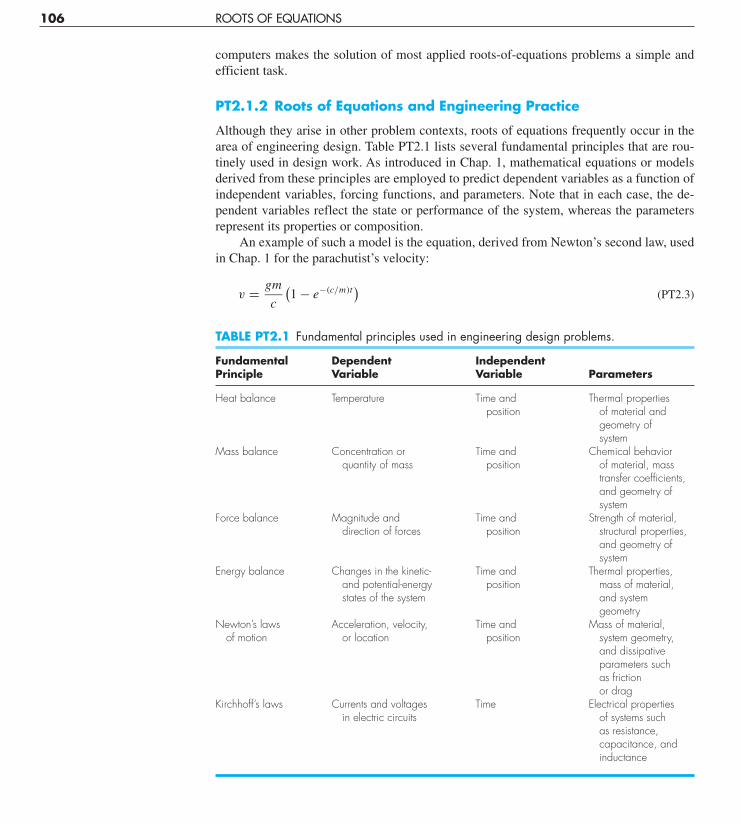
Although they arise in other problem contexts, roots of equations frequently occur in thearea of engineering design. Table PT2.1 lists several fundamental principles that are rou-tinely used in design work. As introduced in Chap. 1, mathematical equations or modelsderived from these principles are employed to predict dependent variables as a function ofindependent variables, forcing functions, and parameters. Note that in each case, the de-pendent variables reflect the state or performance of the system, whereas the parametersrepresent its properties or composition.

An example of such a model is the equation, derived from Newton’s second law, usedin Chap. 1 for the parachutist’s velocity:

v = gm

c

(1 − e−(c/m)t

)(PT2.3)

106 ROOTS OF EQUATIONS

TABLE PT2.1 Fundamental principles used in engineering design problems.

Fundamental Dependent IndependentPrinciple Variable Variable Parameters

Heat balance Temperature Time and Thermal propertiesposition of material and

geometry of system

Mass balance Concentration or Time and Chemical behaviorquantity of mass position of material, mass

transfer coefficients,and geometry ofsystem

Force balance Magnitude and Time and Strength of material,direction of forces position structural properties,

and geometry ofsystem

Energy balance Changes in the kinetic- Time and Thermal properties,and potential-energy position mass of material,states of the system and system

geometryNewton’s laws Acceleration, velocity, Time and Mass of material,

of motion or location position system geometry,and dissipativeparameters suchas friction or drag

Kirchhoff’s laws Currents and voltages Time Electrical propertiesin electric circuits of systems such

as resistance,capacitance, andinductance

cha1873X_p02.qxd 3/21/05 1:01 PM Page 106

where velocity v = the dependent variable, time t = the independent variable, the gravi-tational constant g = the forcing function, and the drag coefficient c and mass m =parameters. If the parameters are known, Eq. (PT2.3) can be used to predict the para-chutist’s velocity as a function of time. Such computations can be performed directlybecause v is expressed explicitly as a function of time. That is, it is isolated on one sideof the equal sign.

However, suppose we had to determine the drag coefficient for a parachutist of a givenmass to attain a prescribed velocity in a set time period. Although Eq. (PT2.3) provides amathematical representation of the interrelationship among the model variables and param-eters, it cannot be solved explicitly for the drag coefficient. Try it. There is no way to re-arrange the equation so that c is isolated on one side of the equal sign. In such cases, c issaid to be implicit.

This represents a real dilemma, because many engineering design problems involvespecifying the properties or composition of a system (as represented by its parameters) toensure that it performs in a desired manner (as represented by its variables). Thus, theseproblems often require the determination of implicit parameters.

The solution to the dilemma is provided by numerical methods for roots of equations.To solve the problem using numerical methods, it is conventional to reexpress Eq. (PT2.3).This is done by subtracting the dependent variable v from both sides of the equation to give

f(c) = gm

c

(1 − e−(c/m)t

) − v (PT2.4)

The value of c that makes f (c) = 0 is, therefore, the root of the equation. This value alsorepresents the drag coefficient that solves the design problem.

Part Two of this book deals with a variety of numerical and graphical methods fordetermining roots of relationships such as Eq. (PT2.4). These techniques can be appliedto engineering design problems that are based on the fundamental principles outlined inTable PT2.1 as well as to many other problems confronted routinely in engineeringpractice.

PT2.2 MATHEMATICAL BACKGROUND

For most of the subject areas in this book, there is usually some prerequisite mathematicalbackground needed to successfully master the topic. For example, the concepts of error es-timation and the Taylor series expansion discussed in Chaps. 3 and 4 have direct relevanceto our discussion of roots of equations. Additionally, prior to this point we have mentionedthe terms “algebraic” and “transcendental” equations. It might be helpful to formally de-fine these terms and discuss how they relate to the scope of this part of the book.

By definition, a function given by y = f(x) is algebraic if it can be expressed in theform

fn yn + fn−1 yn−1 + · · · + f1 y + f0 = 0 (PT2.5)

where fi = an ith-order polynomial in x. Polynomials are a simple class of algebraic func-tions that are represented generally by

fn(x) = a0 + a1x + a2x2 + · · · + an xn (PT2.6)

PT2.2 MATHEMATICAL BACKGROUND 107

cha1873X_p02.qxd 3/21/05 1:01 PM Page 107

where n = the order of the polynomial and the a’s = constants. Some specific examplesare

f2(x) = 1 − 2.37x + 7.5x2 (PT2.7)

and

f6(x) = 5x2 − x3 + 7x6 (PT2.8)

A transcendental function is one that is nonalgebraic. These include trigonometric,exponential, logarithmic, and other, less familiar, functions. Examples are

f(x) = ln x2 − 1 (PT2.9)

and

f(x) = e−0.2x sin(3x − 0.5) (PT2.10)

Roots of equations may be either real or complex. Although there are cases where complexroots of nonpolynomials are of interest, such situations are less common than for polyno-mials. As a consequence, the standard methods for locating roots typically fall into twosomewhat related but primarily distinct problem areas:

1. The determination of the real roots of algebraic and transcendental equations. Thesetechniques are usually designed to determine the value of a single real root on the basisof foreknowledge of its approximate location.

2. The determination of all real and complex roots of polynomials. These methods arespecifically designed for polynomials. They systematically determine all the roots ofthe polynomial rather than determining a single real root given an approximatelocation.

In this book we discuss both. Chapters 5 and 6 are devoted to the first category.Chapter 7 deals with polynomials.

PT2.3 ORIENTATION

Some orientation is helpful before proceeding to the numerical methods for determiningroots of equations. The following is intended to give you an overview of the material inPart Two. In addition, some objectives have been included to help you focus your effortswhen studying the material.

PT2.3.1 Scope and Preview

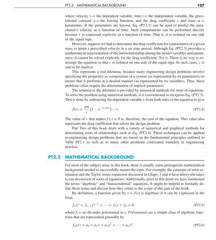
Figure PT2.1 is a schematic representation of the organization of Part Two. Examine thisfigure carefully, starting at the top and working clockwise.

After the present introduction, Chap. 5 is devoted to bracketing methods for findingroots. These methods start with guesses that bracket, or contain, the root and then system-atically reduce the width of the bracket. Two specific methods are covered: bisection andfalse position. Graphical methods are used to provide visual insight into the techniques.Error formulations are developed to help you determine how much computational effort isrequired to estimate the root to a prespecified level of precision.

108 ROOTS OF EQUATIONS

cha1873X_p02.qxd 3/21/05 1:01 PM Page 108

Chapter 6 covers open methods. These methods also involve systematic trial-and-erroriterations but do not require that the initial guesses bracket the root. We will discover thatthese methods are usually more computationally efficient than bracketing methods but thatthey do not always work. One-point iteration, Newton-Raphson, and secant methods aredescribed. Graphical methods are used to provide geometric insight into cases where the

PT2.3 ORIENTATION 109

FIGURE PT2.1Schematic of the organization of the material in Part Two: Roots of Equations.

CHAPTER 5BracketingMethods

PART 2Roots

ofEquations

CHAPTER 6Open

Methods

CHAPTER 7Roots

ofPolynomials

CHAPTER 8EngineeringCase Studies

EPILOGUE

6.5Nonlinearsystems

6.4Multiple

roots

6.3Secant

6.2Newton-Raphson

6.1Fixed-point

iteration

PT 2.2Mathematicalbackground

PT 2.6Advancedmethods

PT 2.5Importantformulas

8.4Mechanicalengineering

8.3Electrical

engineering

8.2Civil

engineering

8.1Chemical

engineering

7.7Libraries and

packages

7.6Other

methods

7.1Polynomials in

engineering

7.2Computing with

polynomials

7.4Muller'smethod

7.5Bairstow's

method7.3

Conventionalmethods

PT 2.4Trade-offs

PT 2.3Orientation

PT 2.1Motivation

5.2Bisection

5.3False

position

5.4Incremental

searches

5.1Graphicalmethods

..

cha1873X_p02.qxd 3/21/05 1:01 PM Page 109

open methods do not work. Formulas are developed that provide an idea of how fast openmethods home in on the root. In addition, an approach to extend the Newton-Raphsonmethod to systems of nonlinear equations is explained.

Chapter 7 is devoted to finding the roots of polynomials. After background sectionson polynomials, the use of conventional methods (in particular the open methods fromChap. 6) are discussed. Then two special methods for locating polynomial roots aredescribed: Müller’s and Bairstow’s methods. The chapter ends with information related tofinding roots with program libraries and software packages.

Chapter 8 extends the above concepts to actual engineering problems. Engineeringcase studies are used to illustrate the strengths and weaknesses of each method and to pro-vide insight into the application of the techniques in professional practice. The applicationsalso highlight the trade-offs (as discussed in Part One) associated with the various methods.

An epilogue is included at the end of Part Two. It contains a detailed comparison of themethods discussed in Chaps. 5, 6, and 7. This comparison includes a description of trade-offs related to the proper use of each technique. This section also provides a summary ofimportant formulas, along with references for some numerical methods that are beyond thescope of this text.

PT2.3.2 Goals and Objectives

Study Objectives. After completing Part Two, you should have sufficient information tosuccessfully approach a wide variety of engineering problems dealing with roots of equa-tions. In general, you should have mastered the techniques, have learned to assess theirreliability, and be capable of choosing the best method (or methods) for any particularproblem. In addition to these general goals, the specific concepts in Table PT2.2 should beassimilated for a comprehensive understanding of the material in Part Two.

Computer Objectives. The book provides you with software and simple computer algo-rithms to implement the techniques discussed in Part Two. All have utility as learning tools.

110 ROOTS OF EQUATIONS

TABLE PT2.2 Specific study objectives for Part Two.

1. Understand the graphical interpretation of a root2. Know the graphical interpretation of the false-position method and why it is usually superior to the

bisection method3. Understand the difference between bracketing and open methods for root location4. Understand the concepts of convergence and divergence; use the two-curve graphical method to

provide a visual manifestation of the concepts5. Know why bracketing methods always converge, whereas open methods may sometimes diverge6. Realize that convergence of open methods is more likely if the initial guess is close to the

true root7. Understand the concepts of linear and quadratic convergence and their implications for the efficiencies

of the fixed-point-iteration and Newton-Raphson methods8. Know the fundamental difference between the false-position and secant methods and how it relates to

convergence9. Understand the problems posed by multiple roots and the modifications available to mitigate them

10. Know how to extend the single-equation Newton-Raphson approach to solve systems of nonlinearequations

cha1873X_p02.qxd 3/21/05 1:01 PM Page 110

Pseudocodes for several methods are also supplied directly in the text. This informa-tion will allow you to expand your software library to include programs that are moreefficient than the bisection method. For example, you may also want to have your ownsoftware for the false-position, Newton-Raphson, and secant techniques, which are oftenmore efficient than the bisection method.

Finally, packages such as Excel, MATLAB software, and program libraries havepowerful capabilities for locating roots. You can use this part of the book to become famil-iar with these capabilities.

PT2.3 ORIENTATION 111

cha1873X_p02.qxd 3/21/05 1:01 PM Page 111