[Year]

Birendra Kumar Project Trainee, IDRBT 3rd Year Undergraduate Integrated M.Sc. Mathematics and Scientific Computing IIT Kanpur Email: biru2k7@gmail.com Project Supervisor: Dr. V. Ravi Associate Professor IDRBT, Hyderabad

SUBMITTED BY

[Type the company name]

[Pick the date]

PARTICLE SWARM OPTIMIZATION BASED NON-

NEGATIVE MATRIX FACTORIZATION AND

APPLICATION TO BANKING

CONTENTS OBJECTIVE

INTRODUCTION

BACKGROUND TO NON-NEGATIVE MATRIX

FACTORIZATION (NMF)

BACKGROUND TO PARTICLE SWARM

OPTIMIZATION (PSO)

PSO ALGORITHM

BACKGROUND TO CREDIT SCORING

REVIEW OF LITERATURE

NMF REVIEW

PSO REVIEW

CREDIT SCORING REVIEW

METHODOLOGY

PROPOSED ALGORITHM

EXPERIMENTS AND RESULTS

CONCLUSION

FUTURE WORK

REFERENCES

OBJECTIVE

The objective of this paper is to implement Non-Negative Matrix factorization (NMF) using Particle Swarm Optimisation (PSO) and apply it to perform feature selection. The hybrid model is used for credit scoring purpose for evaluating the creditworthiness of the credit applicants.

INTRODUCTION

Transparent decision support systems in the finance sector have an important role in the analysis and the decision process. This goal can be achieved only by having a good technical tool to identify creditworthy candidate. The main motivation to apply this approach is to obtain a credit scoring model from a data set that not only have the required performance, but it is relatively interpretable. This objective is achieved through two steps and using complementary soft computing methods. In the first step the original data will be factorize into two non-negative parts using NMF algorithm where PSO will be used to increase the convergence rate and accuracy. And in the second step the reduced data set will be used by different classification algorithms to create a good credit scoring model. The factorization of matrices representing complex multidimensional datasets is the basis of several commonly applied techniques for pattern recognition and unsupervised learning. Similarly to principal components analysis (PCA) or independent component analysis (ICA), the objective of non-negative matrix factorization (NMF) is to explain the observed data using a limited number of basis components, which when combined together approximate the original data as accurately as possible [13]. The distinguishing features of NMF are that both the matrix representing the basis components as well as the matrix of mixture coefficients are constrained to have non-negative entries and that no orthogonality or independence constraints are imposed on the basis components. This leads to a simple and intuitive interpretation of the factors in NMF, and allows the basis components to overlap. The Non-Negative Matrix Factorization (NMF) is an algorithm able to learn a parts-based representation by imposing non negativity constraints that allow only non-subtractive combinations. The idea of using Particle swarm optimisation (PSO) in

finding the non- negative matrix factors came because of fast convergence of PSO over other optimisation techniques. PSO is a population-based optimization tool, which could be implemented and applied easily to solve various function optimization problems, or the problems that can be transformed to function optimization problems. The detailed description of PSO is available in subsequent section.

BACKGROUND TO NON NEGATIVE MATRIX FACTORIZATION

Mathematically, Non-negative Matrix Factorization (NMF) can be described as follows: given an n × m matrix V composed of non-negative elements Vij ≥ 0 where n >> m, the task is to factorize V into a non-negative matrix W of size n × r and another non-negative matrix H of size r × m such that V =WH where r is a pre-specified positive integer that should satisfy the principle r < nm / (n + m). The constrained minimization problem can be put as minimizing the difference between V and WH by: Min f (W, H) = (1/2) ∑ ∑ (Vij – (WH)ij)2

W, H

Subject to Wia≥0 & Hbj≥0 for all i & j. If each column of V represents an object, NMF approximates it by a linear combination of r basis columns in W. The most popular approach to solve this problem seeks to iteratively update the factorization based on a given objective function. This approach is similar to that used in Expectation-Maximization (EM) algorithms and is known as the multiplicative algorithm given below:

NMF Algorithm

input: V ∈ ℝnxm and r = rank

Step 1. Randomize W and H with positive numbers in [0, 1]. Select a cost function to be minimized Step 2. With W fixed, update H, then update W for the updated H. Iterate until the process converges.

Return: W ∈ ℝnxr and H ∈ ℝrxm .

In the above algorithm, the cost function can be of two types,

C1(V,WH) = ||V −WH||f2

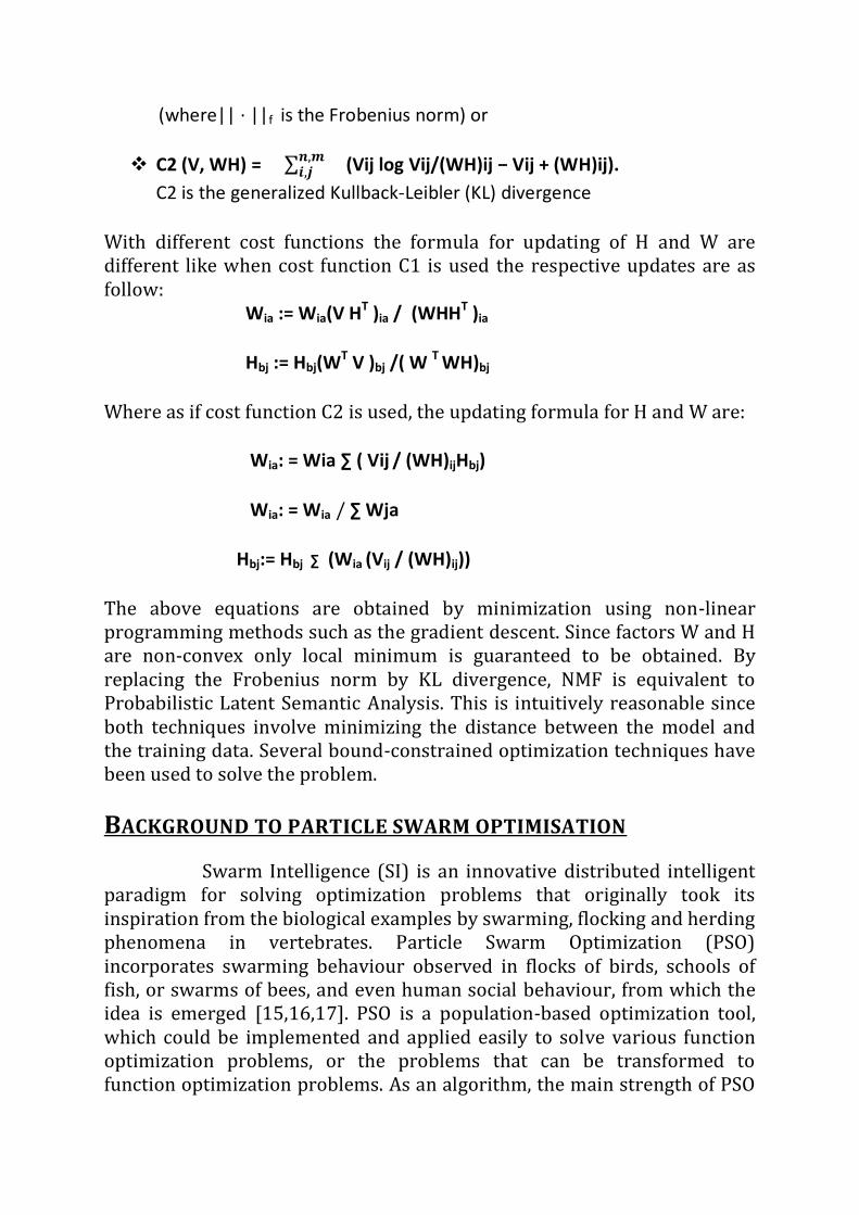
(where|| · ||f is the Frobenius norm) or C2 (V, WH) = 𝒏,𝒎

𝒊,𝒋 (Vij log Vij/(WH)ij − Vij + (WH)ij).

C2 is the generalized Kullback-Leibler (KL) divergence

With different cost functions the formula for updating of H and W are different like when cost function C1 is used the respective updates are as follow: Wia := Wia(V HT )ia / (WHHT )ia

Hbj := Hbj(WT V )bj /( W T WH)bj

Where as if cost function C2 is used, the updating formula for H and W are: Wia: = Wia ∑ ( Vij / (WH)ijHbj) Wia: = Wia / ∑ Wja

Hbj:= Hbj ∑ (Wia (Vij / (WH)ij)) The above equations are obtained by minimization using non-linear programming methods such as the gradient descent. Since factors W and H are non-convex only local minimum is guaranteed to be obtained. By replacing the Frobenius norm by KL divergence, NMF is equivalent to Probabilistic Latent Semantic Analysis. This is intuitively reasonable since both techniques involve minimizing the distance between the model and the training data. Several bound-constrained optimization techniques have been used to solve the problem.

BACKGROUND TO PARTICLE SWARM OPTIMISATION

Swarm Intelligence (SI) is an innovative distributed intelligent paradigm for solving optimization problems that originally took its inspiration from the biological examples by swarming, flocking and herding phenomena in vertebrates. Particle Swarm Optimization (PSO) incorporates swarming behaviour observed in flocks of birds, schools of fish, or swarms of bees, and even human social behaviour, from which the idea is emerged [15,16,17]. PSO is a population-based optimization tool, which could be implemented and applied easily to solve various function optimization problems, or the problems that can be transformed to function optimization problems. As an algorithm, the main strength of PSO

is its fast convergence, which compares favourably with many global optimization algorithms like Genetic Algorithms (GA), Simulated Annealing (SA) and other global optimization algorithms. For applying PSO successfully, one of the key issues is finding how to map the problem solution into the PSO particle, which directly affects its feasibility and performance [16]. In the next section we will see the basic PSO algorithm for solving optimisation problems.

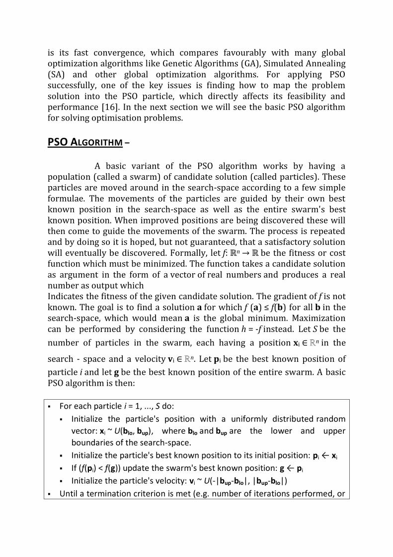
PSO ALGORITHM –

A basic variant of the PSO algorithm works by having a population (called a swarm) of candidate solution (called particles). These particles are moved around in the search-space according to a few simple formulae. The movements of the particles are guided by their own best known position in the search-space as well as the entire swarm's best known position. When improved positions are being discovered these will then come to guide the movements of the swarm. The process is repeated and by doing so it is hoped, but not guaranteed, that a satisfactory solution will eventually be discovered. Formally, let f: ℝn → ℝ be the fitness or cost function which must be minimized. The function takes a candidate solution as argument in the form of a vector of real numbers and produces a real number as output which Indicates the fitness of the given candidate solution. The gradient of f is not known. The goal is to find a solution a for which f (a) ≤ f(b) for all b in the search-space, which would mean a is the global minimum. Maximization can be performed by considering the function h = -f instead. Let S be the

number of particles in the swarm, each having a position xi ∈ ℝn in the

search - space and a velocity vi ∈ ℝn. Let pi be the best known position of

particle i and let g be the best known position of the entire swarm. A basic PSO algorithm is then:

For each particle i = 1, ..., S do:

Initialize the particle's position with a uniformly distributed random

vector: xi ~ U(blo, bup), where blo and bup are the lower and upper

boundaries of the search-space.

Initialize the particle's best known position to its initial position: pi ← xi

If (f(pi) < f(g)) update the swarm's best known position: g ← pi

Initialize the particle's velocity: vi ~ U(-|bup-blo|, |bup-blo|)

Until a termination criterion is met (e.g. number of iterations performed, or

adequate fitness reached), repeat:

For each particle i = 1, ..., S do:

Pick random numbers: rp, rg ~ U(0,1)

Update the particle's velocity: vi ← ω vi + φp rp (pi-xi) + φg rg (g-xi)

Update the particle's position: xi ← xi + vi

If (f(xi) < f(pi)) do:

Update the particle's best known position: pi ← xi

If (f(pi) < f(g)) update the swarm's best known position: g ← pi

Now g holds the best found solution.

The parameters ω, φp, and φg are selected by the practitioner and control

the behaviour and efficacy of the PSO method. In general we take ω as 0ne,

φp and φg as two.

BACKGROUND TO CREDIT SCORING

In the financial industry, consumers regularly request credit to make purchases. The risk for financial institutions to extend the requested credit depends on how well they distinguish the good credit applicants from the bad credit applicants. One widely adopted technique for solving this problem is “Credit Scoring”. Credit scoring is the set of decision models and their underlying techniques that aid lenders in the granting of consumer credit. These techniques decide who will get credit, how much credit they should get, and what operational strategies will enhance the profitability of the borrowers to the lenders. Further, it helps to assess the risk in lending. Credit scoring is a dependable assessment of a person’s credit worthiness since it is based on actual data.

Credit scoring is the most commonly used technique for evaluating the creditworthiness of credit applicants. Its objective is to classify the credit applicants into bad and good customers with respect to their characteristics such as age, income and marital status. Accuracy and transparency are two important criteria that should be satisfied by any credit scoring system. Good accuracy enables correct assessment and thus avoiding any heavy losses associated with wrong predictions while transparency enables financial analysis to understand the decision process. Statistical methods such as linear discriminant analysis (LDA) and logistic regression (LR) are the most commonly used methods in building credit scoring models. However, artificial intelligence like neural networks and

genetic algorithms provide a new alternative to statistical methods in building non-linear, complex and real world systems. Furthermore, techniques using neural networks and genetic algorithms have reported to have achieved higher prediction accuracy than those using LDA and logistic regression and others methods. Many methods have been suggested to develop credit scoring models but the most popular methods adopted in the credit scoring industry are linear discriminant and logistic regression and their variations.

REVIEW OF LITERATURE Various works has been done by different researchers on a variety of research topics using NMF. PSO is also a favourite choice for researchers for solving different kind of optimization problems. These two topics are relatively new than the CREDIT scoring problem. For a long time people are dealing with credit scoring. High investor risk and low consumer satisfaction was the root cause for required improvement in this area. Now researchers are using different techniques for reducing risk and improving satisfaction and they are also successful up to some extent. In the next section we will see how much progress already have been done on these topics.

NON NEGATIVE MATRIX FACTORIZATION Nonnegative Matrix Factorization has been proved to be valuable in many fields of data mining, especially in unsupervised learning. The special point on NMF is its ability to recover the hidden patterns or trends behind the observed data automatically, which makes it suitable for image processing, feature extraction, dimensional reduction and unsupervised learning.

APPLICATION OF NMF

IMAGE PROCESSING Nonnegative Matrix Factorization can trace its

history back to 1970’s, but has attracted lots of attention due to the research of Lee & Seung ([1,2]). In their works, the model was applied to image processing successfully. In image processing, the data can be represented as an n×m nonnegative matrix X, each column of which is an image described by n nonnegative pixel values. Then NMF model can find two factor matrices F and G such that X=FG . F is the so-called basis matrix

since each column can be regarded as a part of the whole such as nose, ear or eye, etc. for facial image data. G is the coding matrix and each row is the weights by which the corresponding image is reconstructed as the linear combination of the columns of F.

CLUSTERING - One of the most interesting and successful applications of

NMF is to cluster data such as text, image or biology data, i.e. discovering patterns automatically from data. Given a nonnegative n×m matrix X, each column of which is a sample and described by n features, NMF can be applied to find two factor matrices F and G such that X = FG, where F is n×r and G is m×r, and r is the cluster number. Columns of F can be regarded as the cluster centroids while G is the cluster membership indicator matrix. In other words, the sample i is of cluster k if Gik is the largest value of the row Gi. The good performance of NMF in clustering has been validated in several different fields including bioinformatics (tumor sample clustering based on microarray data, [3]), community structure detection of the complex network ([4]) and text clustering ([5, 6, 7]).

SEMI SUPERVISED CLUSTERING In many cases, some background

information concerning the pair wise relations of some samples are known and we can add them into the clustering model in order to guide the clustering process. The resulting constrained problem is called semi-supervised clustering. Chen and Rege have incorporated user provided constraints in data clustering [8].

BI-CLUSTERING (CO-CLUSTERING) Bi-clustering was recently introduced

by Cheng & Church [9] for gene expression data analysis. In practice, many genes are only active in some conditions or classes and remain silent under other cases. Such gene-class structures, which are very important to understand the pathology, cannot be discovered using the traditional clustering algorithms. Hence it is very necessary to develop bi-clustering models/algorithms to identify the local structures. Bi-clustering models/algorithms are different from the traditional clustering methodologies which assign the samples into specific classes based on the genes’ expression levels across ALL the samples, they try to cluster the rows (features) and the columns (samples) of a matrix simultaneously. In other words, the idea of bi-clustering is to characterize each sample by a subset of genes and to define each gene in a similar way. As a consequence, bi-clustering algorithms can select the groups of genes that show similar expression behaviours in a subset of samples that belong to some specific classes such as some tumour types, thus identify the local structures of the

microarray matrix data. Binary Matrix Factorization (BMF) was presented for solving bi-clustering problem: the input binary gene-sample matrix X is decomposed into two binary matrices F and G such that X=FGT. The binary matrices F and G can explicitly designate the cluster memberships for genes and samples. Hence BMF offers a framework for simultaneously clustering the genes and samples.

UNDERLYING TRENDS IN STOCK MARKET In the stock market, it has

been observed that the stock price fluctuations does not behave independently of each other but are mainly dominated by several underlying and unobserved factors. Hence try to identify the underlying trends from the stock market data is an interesting problem, which can be solved by NMF. Given an n×m nonnegative matrix X, columns of which is the records of the stock prices during n time points, NMF can be applied to find two nonnegative factors F and G such that X = FGT , where columns of F are the underlying components. Note that identifying the common factors that drive the prices is somewhat similar to blind source separation (BSS) in signal processing. Furthermore, G can be used to identify the cluster labels of the stocks and the most interesting result is that the stocks of the same sector is not necessarily assigned into the same cluster and vice versa, which is of potential use to guide diversified portfolio, in other words, investors should diversify their money into not only different sectors, but also different clusters [10].

DISCRIMINANT FEATURES EXTRACTION IN FINANCIAL DISTRESS DATA

Building appropriate financial distress prediction model based on the extracted discriminative features is more and more important under the background of financial crisis. Ref [11] presents a new prediction model which is indeed a combination of K-means, NMF and support vector machine (SVM). The basic idea is to train a SVM classifier in the reduced dimensional space which is spanned by the discriminative features extracted by NMF, the algorithm of which is initialized by K-means. The details can be found in ref [11]. In summary, NMF can discover the common basis hidden behind the observations and the way how the images are reconstructed by the basis. But further researches have also shown that the standard NMF model does not necessarily give the correct part of whole representations, hence many efforts have been done to improve the sparseness of NMF in order to identify more localized features that are building parts for the whole representation.

PARTICLE SWARM OPTIMIZATION-

Particle Swarm Optimization (PSO), in its present form, has been in existence for roughly a decade, with formative research in related domains (such as social modelling, computer graphics, simulation and animation of natural swarms or flocks) for some years before that; a relatively short time compared with some of the other natural computing paradigms such as artificial neural networks and evolutionary computation. However, in that short period, PSO has gained widespread appeal amongst researchers and has been shown to offer good performance in a variety of application domains, with potential for hybridisation and specialisation, and demonstration of some interesting emergent behaviour.

CREDIT SCORING

Before credit scoring models came into wide use in 1980, human judgment was the sole factor in making decisions who are the good and bad applicants, and then who receive credit. Judgmental method was not only slow but also unreliable because of the human error and bias.

Credit scoring models nowadays are based on statistical or operation research methods. These models are built using payment historical information from thousands of actual consumers. Credit scoring objective is to assign credit applicants to either good customers or bad customers. Therefore credit scoring lies in the domain of the classification problem [12]. The credit scoring model captures the relationship between the historical information and future credit performance. This relation can be described mathematically as follows:

f (x1, x2,..., xm) = yn Where each customer contains attributes: x1, x2,..., xm, yj , denotes the type of customer, for example good or bad is the function or the credit scoring model that maps between the customer features (inputs) and his creditworthiness (output). The task of the credit scoring model (function) is to predict the value of - i.e. the creditworthy of customer i - by knowing the .i.e. the customer features such as: income, age. Many methods have been suggested to develop credit scoring models but the most popular

methods adopted in the credit scoring industry are linear discriminant and logistic regression and their variations [13].

CREDIT SCORING MODEL

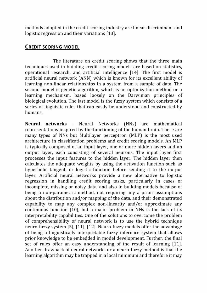
The literature on credit scoring shows that the three main techniques used in building credit scoring models are based on statistics, operational research, and artificial intelligence [14]. The first model is artificial neural network (ANN) which is known for its excellent ability of learning non-linear relationships in a system from a sample of data. The second model is genetic algorithm, which is an optimization method or a learning mechanism, based loosely on the Darwinian principles of biological evolution. The last model is the fuzzy system which consists of a series of linguistic rules that can easily be understood and constructed by humans. Neural networks - Neural Networks (NNs) are mathematical representations inspired by the functioning of the human brain. There are many types of NNs but Multilayer perceptron (MLP) is the most used architecture in classification problems and credit scoring models. An MLP is typically composed of an input layer, one or more hidden layers and an output layer, each consisting of several neurons. The input layer first processes the input features to the hidden layer. The hidden layer then calculates the adequate weights by using the activation function such as hyperbolic tangent, or logistic function before sending it to the output layer. Artificial neural networks provide a new alternative to logistic regression in handling credit scoring tasks, particularly in cases of incomplete, missing or noisy data, and also in building models because of being a non-parametric method, not requiring any a priori assumptions about the distribution and/or mapping of the data, and their demonstrated capability to map any complex non-linearity and/or approximate any continuous function [10], but a major problem in NNs is the lack of its interpretability capabilities. One of the solutions to overcome the problem of comprehensibility of neural network is to use the hybrid technique neuro-fuzzy system [5], [11], [12]. Neuro-fuzzy models offer the advantage of being a linguistically interpretable fuzzy inference system that allows prior knowledge to be embedded in model development. Further, the final set of rules offer an easy understanding of the result of learning [11]. Another drawback of neural networks or a neuro-fuzzy method is that the learning algorithm may be trapped in a local minimum and therefore it may

never find the global solution. Genetic Algorithms are shown [13] to be suitable tools for determining the optimal topology of a neural network. Genetic algorithm -Genetic algorithm (GA) searches for the optimal solution by a number of modifications of strings of bits called chromosomes. The chromosomes are the encoded form of the parameters of the given problem. In successful iterations (generations), the chromosomes are modified in order to find the chromosome corresponding to the maximum of the fitness function. Each generation consists of three phases: reproduction, crossover, and mutation.

Fuzzy system - The term “fuzzy systems” refers mostly to systems that are governed by fuzzy IF–THEN rules such as: IF temperature is cold THEN set output of the heater High The IF part of an implication is called the antecedent whereas the second, THEN part is a consequent. A fuzzy system is a set of fuzzy rules that converts inputs to outputs. The fuzzy inference engine combines fuzzy IF–THEN rules into a mapping from fuzzy sets in the input space X to fuzzy sets in the output space Y based on fuzzy logic principles. The number of rules increases exponentially with the dimension of the input space (number of system variables). This rule explosion is called the principle of dimensionality and is a general problem for mathematical models. For the last five years several approaches based on decomposition (cluster) merging and fusing have been proposed to overcome this problem.

METHODOLOGY In this paper we have chosen Frobenious norm as the cost

function and our objective is to minimize this cost function with non

negativity constraints on factors. Let p denotes the swarm population and

f: ℝn → ℝ be our cost function, V∈ ℝnxm is original normalised data matrix

which we want to factorise, W∈ ℝnxr and H∈ ℝrxm be the two factors where

r<(nm/n+m ) then the proposed algorithm is then:

Proposed Algorithm

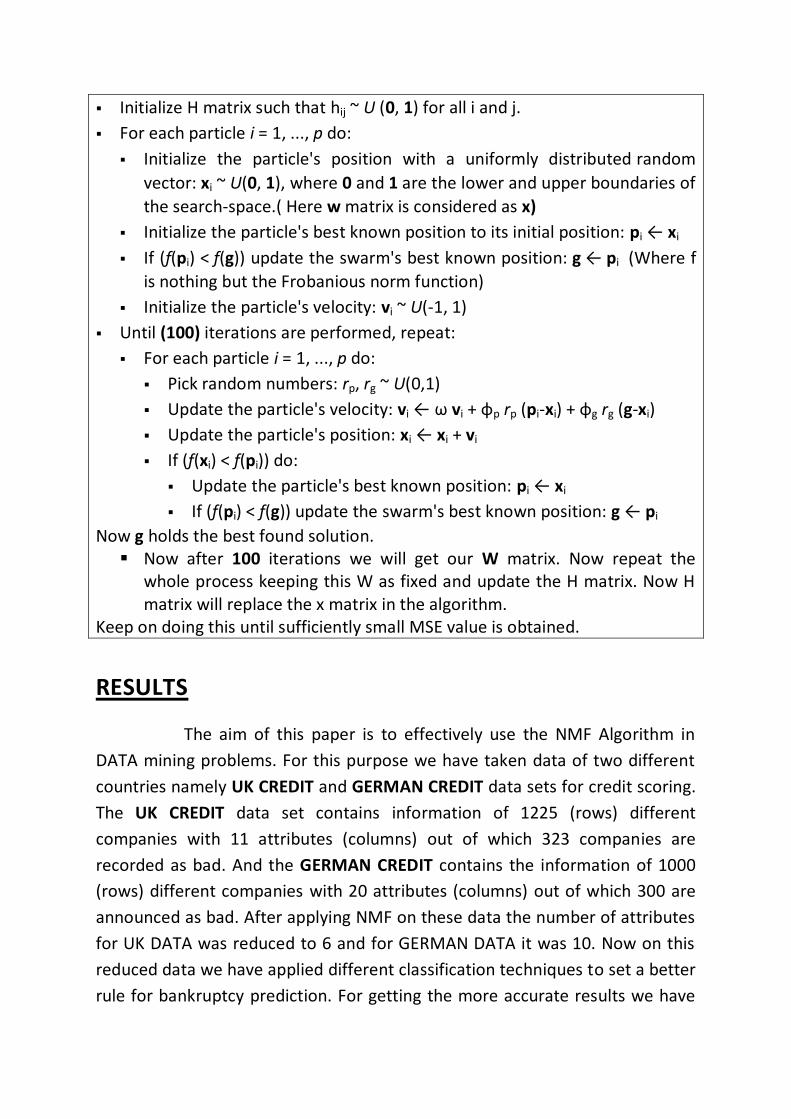
Initialize H matrix such that hij ~ U (0, 1) for all i and j.

For each particle i = 1, ..., p do:

Initialize the particle's position with a uniformly distributed random

vector: xi ~ U(0, 1), where 0 and 1 are the lower and upper boundaries of

the search-space.( Here w matrix is considered as x)

Initialize the particle's best known position to its initial position: pi ← xi

If (f(pi) < f(g)) update the swarm's best known position: g ← pi (Where f

is nothing but the Frobanious norm function)

Initialize the particle's velocity: vi ~ U(-1, 1)

Until (100) iterations are performed, repeat:

For each particle i = 1, ..., p do:

Pick random numbers: rp, rg ~ U(0,1)

Update the particle's velocity: vi ← ω vi + φp rp (pi-xi) + φg rg (g-xi)

Update the particle's position: xi ← xi + vi

If (f(xi) < f(pi)) do:

Update the particle's best known position: pi ← xi

If (f(pi) < f(g)) update the swarm's best known position: g ← pi

Now g holds the best found solution. Now after 100 iterations we will get our W matrix. Now repeat the

whole process keeping this W as fixed and update the H matrix. Now H matrix will replace the x matrix in the algorithm.

Keep on doing this until sufficiently small MSE value is obtained.

RESULTS

The aim of this paper is to effectively use the NMF Algorithm in

DATA mining problems. For this purpose we have taken data of two different

countries namely UK CREDIT and GERMAN CREDIT data sets for credit scoring.

The UK CREDIT data set contains information of 1225 (rows) different

companies with 11 attributes (columns) out of which 323 companies are

recorded as bad. And the GERMAN CREDIT contains the information of 1000

(rows) different companies with 20 attributes (columns) out of which 300 are

announced as bad. After applying NMF on these data the number of attributes

for UK DATA was reduced to 6 and for GERMAN DATA it was 10. Now on this

reduced data we have applied different classification techniques to set a better

rule for bankruptcy prediction. For getting the more accurate results we have

used tenfold cross validation technique. The tenfold result obtained for these

two data sets are as follow:

Classification Method

UK CREDIT data

GERMAN CREDIT data

DT 66.14% 60.8%

MLP 73.0% 61.8%

kNN 67.22% 65.4%

RF 70.29% 64.2%

CART 69.16% 67.9%

SVM 73.63% 70.0%

logistic 73.63% 70.0%

CONCLUSION:-

In this paper we have applied NMF on UK CREDIT data sets and

GERMAN CREDIT data set to achieve our goal of dimension reduction and after

successfully achieving the goal we have applied different classification

algorithms like SVM, PNN, KNN, DECISION TREE, SIMPLE CART and MLP on

these data for credit scoring. In UK data all classification techniques are giving

better results compare to GERMAN data. And LOGISTIC, SVM, MLP and RF are

giving better accuracy than CART and KNN in UK data.

REFERENCES: -

[1] D. D. Lee and H. S. Seung. Learning the parts of objects by non-negative matrix factorization. Nature, 401(6755):788–791, October 1999. [2] Daniel D. Lee and Sebastian H. Seung. Algorithms for non-negative matrix factorization. In Annual Conference on Neural Information Processing Systems, pages 556–562, 2000 [3] J. P. Brunet, P. Tamayo, T. R. Golub, and J. P. Mesirov. Metagenes and molecular pattern discovery using matrix factorization. Proc Natl Acad Sci U S A, 101(12):4164–4169, March 2004. [4]Bo Long, Xiaoyun Wu, Zhongfei Zhang, and Philip S. Yu. Community learning by graph approximation. In Proceedings of the 8th IEEE International Conference on Data Mining. ICDM 2007, 2007. [5]V. Paul Pauca, Farial Shahnaz, Michael W. Berry, and Robert J. Plemmons. Text mining using non-negative matrix factorizations. In Proceedings of the Fourth SIAM International Conference on Data Mining, 2004. [6] Farial Shahnaz, Michael W. Berry, Pauca, and Robert J. Plemmons. Document clustering using nonnegative matrix factorization. Information Processing & Management, 42(2):373– 386, March 2006. [7] Wei Xu, Xin Liu, and Yihong Gong. Document clustering based on non-negative matrix factorization. In SIGIR ’03: Proceedings of the 26th annual international ACM SIGIR conference on Research and development in informaion retrieval, pages 267–273, New York, NY, USA, 2003. ACM Press. [8] Yanhua Chen, Manjeet Rege, Ming Dong, and Jing Hua. Incorporating user provided constraints into document clustering. In ICDM ’07: Proceedings of the 2007 Seventh IEEE International Conference on Data Mining, pages 103–112, Washington, DC, USA, 2007. IEEE Computer Society. [9] Yizong Cheng and George M. Church. Biclustering of expression data. In Proceedings of the Eighth International Conference on Intelligent Systems for Molecular Biology, pages 93–103. AAAI Press, 2000.

[10] Konstantinos Drakakis, Scott Rickard, Ruairi de Frein, and Andrzej Cichocki. Analysis of financial data using non-negative matrix factorization. International Mathematical Forum, 3(38):1853–1870, 2008. [11] Bernardete Ribeiro, Catarina Silva, Armando Vieira, and João Carvalho das Neves. Extracting discriminative features using non-negative matrix factorization in financial distress data. In ICANNGA, pages 537–547, 2009. [12] S. Piramuthu , “Financial credit-risk evaluation with neural and neurofuzzy systems”. European Journal of Operational Research, 112, pp. 310–321 (1999). [13] Desai, V., Crook, J., & Overstreet, G. Credit scoring models in the credit union environment using neural networks and genetic algorithms. IMA Journal of Mathematics Applied in Business and Industry, 8(4), 324–346 (1997). [14] L.C. Thomas, “A survey of credit and behavioral scoring: Forecasting financial risks of lending to customers”, International Journal of Forecasting, vol 16, pp. 149–172 (2000). [15] Kennedy J and Eberhart R (2001) Swarm intelligence. Morgan Kaufmann Publishers, Inc., San Francisco, CA. [16] Clerc M and Kennedy J (2002) The particle swarm-explosion, stability, and convergence in a multidimensional complex space. IEEE Transactions on Evolutionary Computation, 6(1):58-73.

[17]Pang W, Wang K P, Zhou C G, at el. (2004) Fuzzy discrete particle swarm optimization for solving traveling salesman problem. Proceedings of the 4th International Conference on Computer and Information Technology, IEEE CS Press.