particle physics models with four generations -...
TRANSCRIPT
Pro gradu -tutkielmaTeoreettinen fysiikka
Particle physics models with four generations
Hanna Grönqvist2012
Ohjaaja: Prof. Katri HuituTarkastajat: Prof. Katri Huitu
Prof. Paul Hoyer
HELSINGIN YLIOPISTOFYSIIKAN LAITOS
PL 64 (Gustaf Hällströmin katu 2)00014 Helsingin yliopisto

2
Contents
I Perliminaries 5
1 Motivation 7
1.1 Historical overview – the ‘discovery’ of the standard model . . . . . . . . . . . . . . . 7
1.2 Problems of the standard model solved by a fourth generation . . . . . . . . . . . . . 10
1.2.1 Naturalness . . . . . . . . . . . . . . . . . . . . . . . . . . . . . . . . . . . . . 12
1.2.2 Flavor democracy – a solution to the naturalness problem . . . . . . . . . . . 14
1.2.3 Electroweak Precision Data . . . . . . . . . . . . . . . . . . . . . . . . . . . . 15
1.3 Unitarity constraints on the fourth generation . . . . . . . . . . . . . . . . . . . . . . 17
2 The Standard Model 21
2.1 Quantum chromodynamics . . . . . . . . . . . . . . . . . . . . . . . . . . . . . . . . . 21
2.1.1 Gauge fixing and Faddeev–Popov ghosts . . . . . . . . . . . . . . . . . . . . . 22
2.1.2 Renormalization and asymptotic freedom . . . . . . . . . . . . . . . . . . . . 24
2.2 Local SU(2) and U(1) symmetries . . . . . . . . . . . . . . . . . . . . . . . . . . . . 25
2.2.1 Isospin symmetry . . . . . . . . . . . . . . . . . . . . . . . . . . . . . . . . . . 25
2.2.2 Quantum electrodynamics . . . . . . . . . . . . . . . . . . . . . . . . . . . . . 26
2.3 Spontaneous symmetry breaking . . . . . . . . . . . . . . . . . . . . . . . . . . . . . 26
2.3.1 The Higgs mechanism . . . . . . . . . . . . . . . . . . . . . . . . . . . . . . . 27
2.4 The Glashow–Weinberg–Salam model . . . . . . . . . . . . . . . . . . . . . . . . . . 29
2.5 Quark and lepton mixing . . . . . . . . . . . . . . . . . . . . . . . . . . . . . . . . . 31
2.5.1 The quark sector . . . . . . . . . . . . . . . . . . . . . . . . . . . . . . . . . . 31
2.5.2 Beyond the SM: mixing in the lepton sector . . . . . . . . . . . . . . . . . . . 33
II The minimal four–generation model 39
3 Phenomenology of the fourth family 41
3.1 Mixing of the fourth family with the first three ones . . . . . . . . . . . . . . . . . . 41
3.1.1 Sources for constraints . . . . . . . . . . . . . . . . . . . . . . . . . . . . . . . 41
3.1.2 Possible parameter space . . . . . . . . . . . . . . . . . . . . . . . . . . . . . . 43
3.2 Higgs production and partial decay widths . . . . . . . . . . . . . . . . . . . . . . . . 47
3.2.1 Higgs production at hadron colliders . . . . . . . . . . . . . . . . . . . . . . . 47
3.2.2 Branching fractions . . . . . . . . . . . . . . . . . . . . . . . . . . . . . . . . . 51
3.2.3 Searches for the Higgs and the fourth family . . . . . . . . . . . . . . . . . . . 53
3
4 CONTENTS
4 Experimental searches 57
4.1 Search strategies – SM4 quarks . . . . . . . . . . . . . . . . . . . . . . . . . . . . . . 574.1.1 General event topologies . . . . . . . . . . . . . . . . . . . . . . . . . . . . . . 574.1.2 Pair production of fourth family quarks . . . . . . . . . . . . . . . . . . . . . 584.1.3 Single production of fourth family quarks . . . . . . . . . . . . . . . . . . . . 594.1.4 Current experimental bounds . . . . . . . . . . . . . . . . . . . . . . . . . . . 64
4.2 Searches for fourth generation leptons . . . . . . . . . . . . . . . . . . . . . . . . . . 664.2.1 Neutrinos and Higgs at the LHC . . . . . . . . . . . . . . . . . . . . . . . . . 674.2.2 Searches at future lepton colliders . . . . . . . . . . . . . . . . . . . . . . . . . 684.2.3 Existing experimental constraints . . . . . . . . . . . . . . . . . . . . . . . . . 70
4.3 Higgs searches . . . . . . . . . . . . . . . . . . . . . . . . . . . . . . . . . . . . . . . . 714.3.1 Higgs searches at Tevatron . . . . . . . . . . . . . . . . . . . . . . . . . . . . 714.3.2 Higgs searches at the LHC . . . . . . . . . . . . . . . . . . . . . . . . . . . . . 72
5 Experimental exclusion of the minimal SM4 75
III The two Higgs doublet model 79
6 Theory of the 2HDM 81
6.1 Why add another doublet? . . . . . . . . . . . . . . . . . . . . . . . . . . . . . . . . . 816.2 The scalar potential and the field content . . . . . . . . . . . . . . . . . . . . . . . . 826.3 Flavor conservation . . . . . . . . . . . . . . . . . . . . . . . . . . . . . . . . . . . . . 836.4 Yukawa couplings of the type II 2HDM . . . . . . . . . . . . . . . . . . . . . . . . . . 84
7 4F2HDM phenomenology 85
7.1 Higgs production and decay in the 2HDM–II . . . . . . . . . . . . . . . . . . . . . . 857.1.1 Production and decay of the neutral pseudoscalar A0 . . . . . . . . . . . . . . 867.1.2 Production and decay of the light neutral Higgs h0 . . . . . . . . . . . . . . . 887.1.3 The charged Higgs . . . . . . . . . . . . . . . . . . . . . . . . . . . . . . . . . 89
7.2 Searches for the 4F2HDM at the LHC . . . . . . . . . . . . . . . . . . . . . . . . . . 917.2.1 Fourth generation quarks masses . . . . . . . . . . . . . . . . . . . . . . . . . 91
8 Conclusions 95
Appendices 97
A Definitions of electroweak observables 99
B The Goldstone model 101
C Mathematical description of neutrino oscillations 105
D Oblique electroweak parameters 107
E Feynman diagrams for production of fourth family particles 113
F Form factors for A0, h0 branching ratios 117
Bibliography 119
Part I
Perliminaries
5

Chapter 1
Motivation
In this chapter we will shortly review the historical development of the Standard Model of elementaryparticle physics. The aim of the historical overview is to give an idea as to how the current theory wasborn, from theoretical predictions and experimental verification with many unexpected discoveriesleading to reformulations and expansions of the theory. With this section we wish to show the readerthat there have been unexpected events along the way: that there might still be many surprises instore for us and that it might be premature to think that our current view of particle physics iscomplete.
In the second part of this chapter we list some shortcomings of the current model, called the‘standard model’, and give some arguments in favor of adding a fourth family of particles. Ideaspresented in this section will be considered in some detail later on in the text.
1.1 Historical overview – the ‘discovery’ of
the standard model
The observable matter of the universe consists of atoms that are made up of protons, neutrons andelectrons. All of these particles were discovered in the 1930’s, and at the time they were deemed tobe elementary constituents, just as had been thought of atoms before that. Before this the photonhad also been found, the photon being the quantum of the electromagnetic field that ‘binds’ theelectron to the atomic nucleus. The force binding the protons and neutrons of the nucleus wasthought to be mediated by a particle called the ‘pi-meson’, as suggested by Yukawa [1]. WhenPauli predicted the existence of one more particle, the electron neutrino, as a solution to a problem(missing energy in beta decays) [2], it appeared that a complete picture of particle physics had beenestablished.
The situation changed when the muon was discovered some years later, in 1937 [3, 4]. The muonseemed identical to the electron, but with 200 times its mass. It was also very puzzling that thisnew particle seemed to be produced by strong interactions but its interactions with matter wereelectromagnetic. A famous physicist, Rabi, then made a comment conveying the amazement at thissurprise, cited many times since: ‘Who ordered that?’ [5].
Ten years later the charged pion, predicted by Yukawa, was found [6, 7, 8]. At the same timeanother meson was discovered, too [9]. Later it became clear that this was similar to Yukawa’sparticle, but neutral, and so it became known as the ‘neutral pion’ [10]. These new pieces fit intoa beautifully simple theory where electromagnetic interactions are mediated by photons, stronginteractions by π-mesons and weak interactions are described by the Fermi four-fermion interaction;all nuclei are bound states of protons and neutrons, atoms bound states of nuclei and electrons and
7
8 CHAPTER 1. MOTIVATION
the matter fields classified as leptons (electron and its neutrino), mesons (the pions) and baryons(consisting of protons and neutrons).
The beginning of a new decade, the 50’s, opened a new ‘era’ of elementary particle physics [5, 11]:In 1951, cloud chamber observations showed a new neutral particle (Λ), which decayed into aproton and a negative pion; in 1952-1953 the negatively charged Ξ and the charged Σ-particleswere detected in cosmic rays at high altitudes. All of these (later called hyperons) were heavierthan the known nucleons and exhibited an unusual feature: they were produced relatively often innuclear collisions, but then they decayed with long life-times of O(10−10) − O(10−8) s, suggestingthat they were produced in strong interactions but decayed through weak ones. These particles,called ‘strange’ and always produced in pairs led to the discovery of the strange quark [12, 13, 9]. Atheoretical explanation was given both by Nakano and Nishijima [14] in Japan, and independentlyGell-Mann [15] in the USA. As a part of this explanation they introduced a new quantum numbercalled ‘strangeness’, related to other, already established, quantum numbers.
In the following years there was a great accumulation of data on baryon and meson resonancesas a consequence of the completion and running of several particle accelerators. By the mid-1960’s it was realized that the contemporary theory did not suffice as an explanation for the manynew particles that were being discovered. The idea of quarks as the constituents of mesons andbaryons was put forward by Gell-Mann [16] and Zweig [17] in 1964. Further the notion of ‘colorcharge’ was introduced in 1964 by Greenberg [18] and in 1965 by Nambu and Han [19]. Sinceleptons were observed to have a specific pattern, emanating from the discovery of the muon andmuon neutrino [20], a fourth quark was predicted in 1964 by Bjorken and Glashow [21], an ideathat was further worked on by Glashow, Iliopoulos and Maiani [22] in 1970. It was recognizedthat the fourth quark allowed for a theory with flavor conserving neutral currents, but not flavorchanging ones (called the ‘GIM’ mechanism), as explained by two generations related throughCabibbo mixing [23]. This model was consistent with observations and the fourth quark, called‘charm’, was found in 1974 [24, 25, 26, 27]. By this time a renormalizable gauge theory had beendeveloped [28, 29, 30, 31], based on the two ‘generations’ of particles observed thus far, the firstgeneration being the u and d quarks, the electron and its neutrino and the second generationconsisting of the c and s quarks, the muon and its neutrino.
A quantum field theory of strong interactions was formulated in 1973, first suggested by Fritzsch,Gell-Man and Leutwyler [32]. Quarks were deemed to be real particles (as opposed to mere mathe-matical tool) carrying a charge of their own – the ‘color’ charge. In this theory of color interactions,called quantum chromodynamics (QCD), the massless quanta of the color field were named gluons.A very peculiar feature of the theory was discovered not long afterwards – a property later called‘asymptotic freedom’, needed to describe observed properties of the proton [33, 34, 35, 36, 37].
As had been the case for the theory based on just one family of particles, the theory basedon two families suddenly experienced severe problems with the experimental discovery of the taulepton in 1975 [38]. Two years later, in 1977, a fifth quark, named ‘bottom’, was discovered [39, 40].The search for a sixth quark went on for 18 years and it was only when the Fermilab acceleratorTevatron reached sufficiently high energies that the unexpectedly heavy top quark was found in1995 [41, 42], with a mass much larger than that of the bottom quark.
The last particle of the third generation, the tau neutrino was finally found in 2000 [43].
This brief review of the ‘discovery’ of particle physics is meant to show the reader that therehas been an abundance of surprises in the history of particle physics. Especially, the discovery ofparticles belonging to a new generation has already on two occasions, in the case of the second andthe third families, come as a surprise. When the history of new and unexpected discoveries is taken

1.1. HISTORICAL OVERVIEW – THE ‘DISCOVERY’ OF THE STANDARD MODEL 9
into account, it might well be that, even though the situation has been ‘stable’ for many years, westill do not know the whole story.
That there are only three families of particles is an idea that has been generally accepted forsome time. The origin of this idea lies in the precision tests made at LEP, showing with highstatistical significance that the number of light neutrinos is three. This ‘has led to the prevalent,if rather optimistic, belief that ... the number of sequential lepton and quark families has alsobeen determined to be 3’ [44]. But then again ‘this belief hinges on the notion that a heavysequential Dirac neutrino (mν ≫ mZ/2) belonging to a possible fourth generation would necessarilyimply an unnaturally large hierarchy among the Yukawa couplings of different neutrinos with theHiggs boson’ [44]. In sections to come, we will see that the masses of elementary particles aredescribed through the particles’ Yukawa interactions with a field called the Higgs field. ‘Unnaturallylarge hierarchy’ among the couplings here refers to the fact that the known particles have verydifferent masses. ‘Though the naturalness argument is intuitively rather appealing, it is basically aphilosophical outlook and hence is not beyond debate’ [44].
A further similar, more specific argument four the three families of particles is that one wouldnot expect a neutrino to be so heavy as to not be seen in the LEP measurements of the Z boson.This argument has been countered by a wise comment: “the necessarily heavy neutrino mass,mnu4
> mZ/2, would be surprising, but without a theory of neutrino masses we are not really in aposition to judge” [45].
10 CHAPTER 1. MOTIVATION
1.2 Problems of the standard model solved by
a fourth generation
Although the standard model [46, 28, 31] with three generations (to be denoted ‘SM3’) has beenimmensely successful in describing the strong and electroweak interactions of elementary particlesthere are still some issues that it does not cover in a satisfactory way. Many physicists today believethat the SM3 is not the ‘ultimate’ theory, but rather an effective theory which is applicable at lowenergies only. In this sense the SM is thought to be just the low energy limit of a more fundamental,underlying theory. A variety of ‘beyond the standard model’ (BSM) theories have been proposed totake the role of this underlying, more extensive theory. Such BSM models are e.g. theories includingsupersymmetry or extra dimensions or even string theory and grand unified theories. A possibleway to extend the standard model, so that it might better explain observed phenomena is to add asequential fourth chiral family to the three already known families of elementary particles. This isa very simple and perhaps a very ‘natural’ way to extend the SM, and it is the topic of this thesis.This model will henceforth be referred to as ‘SM4’.
The motivation for the development of the various BSM models is the fact that some of thetheoretical aspects of the SM are not well understood, seem to be lacking a fundamental explanationor are not yet experimentally verified. Another problem is that there are some experimentallyobserved phenomena that exhibit some tension with the SM predictions. Amongst these openissues are for example :
1. Origin of mass
2. Quark-lepton symmetry
3. Family replication and number of families
4. Masses and mixing pattern of fermions
5. Violation of parity
6. Baryon asymmetry of the universe
7. Large number of arbitrary parameters
The origin of mass is a question of fundamental importance to particle physics. As we will latersee (in Section 2.3), the masses of all particles are thought to arise from their interactions witha scalar field. These interactions are called ‘Yukawa interactions’ and the scalar field is called the‘Higgs field’. The SM predicts some of the properties of the Higgs particle, the quantum of the Higgsfield, but it does not predict its mass. Short-lived particles that live such a short time that theycannot be directly seen, are instead indirectly observed in detectors through their decay products.A motivation for SM4 is that the presence of a massive fourth generation would affect the Higgsboson cross sections and decay channels.
At the moment there is some tension between the SM fit to and the lower bound on the Higgsboson mass as measured by LEP II. It is not known whether the two anomalies giving rise to thistension arise from unknown physics or if they are just due to systematic errors. If these anomaliesare removed, the SM fit improves, but then the predicted Higgs mass falls into a region alreadyexcluded by LEP giving a contradiction. When the anomalies are present, then the SM fit is badand this situation is not satisfactory either. Interestingly, if a fourth family is added, then the fit
1.2. PROBLEMS OF THE STANDARD MODEL SOLVED BY A FOURTH GENERATION 11
gets better, giving a reason to study such a model. [47] We come later (in Chapter 5) to the issueof an observed 125 GeV boson at the LHC.
A further thing about the fourth family and the origin of mass is that, in addition to theeffect the fourth generation particles have on the Higgs field, they could also be the initiators ofelectroweak symmetry breaking themselves. This would be possible if the Yukawa couplings of thefourth generation particles were found to be very big because then they could dynamically breakthe electroweak symmetry [48].
The idea that there are three SM families has been widely accepted for a long time. This beliefis based on SLAC [49, 50] and LEP [51, 52, 53, 54] data of the width of the Z boson peak. Asnoted in Ref. [54]: “In the standard electroweak model the Z boson is expected to decay withcomparable probability into all species of fermions that are kinematically allowed. The decay rateof the Z into light, neutral, penetrating particles such as neutrinos, that would otherwise escapedetection, can be measured through an increase in the total width ΓZ ”. The visible width fromexperimentally measured decay channels can be subtracted to give the ‘invisible’ width, that of theneutrino channels. The results of the measurements at electron–positron colliders is that there areonly three light (mν ≪ mZ/2) neutrinos [55]:
Number of light neutrino types : 2.9840 ± 0.0082 at 95% C.L. (1.1)
with ‘C.L.’ standing for confidence level (or limit).
The generally accepted conclusion drawn from these results was that there could thus onlyexist three generations of particles in the SM. Yet, as already mentioned in the previous section,this conclusion relies upon the thought that a heavy fourth neutrino would not be ‘natural’, andthat its presence (along with the other, probably heavy, particles of the fourth generation) wouldlead to ‘unnaturally’ large differences in the masses of all the elementary particles. But in fact anunnatural hierarchy is not inevitable for the existence of a heavy fourth neutrino: actually the mostnatural scenario can be implemented in a four family model [44]. This is the case if there are three(nearly) massless neutrinos and a heavy neutrino, as given by the democratic mass matrix in thehypothesis of flavor democracy (see Section 1.2.2). This hypothesis is in agreement with a verysimple conclusion of the Z width (1.1): that there are at least three generations.
As it is, the SM does not give a theoretical prediction for the number of families. Each SM familyis independently anomaly-free and therefore the number of families is completely unrestricted in thesense of theoretical consistency of the model. The only restriction coming from the SM is an upperlimit given by the asymptotic freedom of Quantum Chromodynamics (QCD) [35], which requiresthe number of generations to be less than or equal to eight. There are also some other hintsof an upper limit, namely some considerations that seem to disfavor a fifth sequential family. Ifone assumes flavor democracy, then a fifth family would lead to four massless or nearly masslessneutrinos and one heavy one but this contradicts (1.1), and is therefore improbable. One wouldalso expect mt ≪ mt′ ≪ mt′′ , where mt is the top quark mass (mt ∼ 175 GeV) and t′ and t′′ referto the top type quarks of the fourth and fifth generation respectively. In this scenario mt′ is alreadyclose to the unitarity limit, and therefore the theory is no longer trustworthy for energies as high asmt′′ . [56]
Finally, we note that a fourth family could give an explanation to one of the open questions incosmology, concerning the ratio of matter to antimatter in the observable universe. A fourth familycould contribute with a factor up to O(1010) [57] or possibly from O(1013) to O(1015) [58] to thebaryon asymmetry of the universe, thus giving the observed amount of baryons to antibaryons inthe universe, a ratio that that SM3 predicts to be much too small.
12 CHAPTER 1. MOTIVATION
1.2.1 Naturalness
As far as has been experimentally found to date, there exists three families or generations of particles.In the standard model, to be reviewed in the next chapter, the elementary particles are groupedinto doublets of the SU(2) gauge group.
ith generation : quarks
(uidi
)and leptons
(ℓiνi
), (1.2)
with
ui = u, c, t , di = d, s, b , ℓi = e, µ, τ , νi = νe, νµ, ντ , (1.3)
for i = 1, 2, 3. The quarks of a family form one doublet and the leptons another.The masses of all particles are created in the same way – through the Higgs mechanism. One
might think that this would imply that all masses are of the same order of magnitude, but thisturns out not to be the case. From experiments we know that [59]
(mu ≈ 2.3 MeVmd ≈ 4.8 MeV
),
(mc ≈ 1.3 GeVms ≈ 95 MeV
),
(mt ≈ 173 GeVmb ≈ 4 GeV
), (1.4)
(me ≈ 2.3 MeVmνe < 225 eV
),
(mµ ≈ 1, 275 GeVmνµ < 0.19 MeV
),
(mτ ≈ 173 GeVmντ < 18.2 MeV
). (1.5)
Eqs. (1.4), (1.5) show that the masses of each generation increase, the first generation being thelightest one, the third the heaviest one. The mass gap between sequential generations is often calledthe flavor problem.
The large mass differences are surprising, since one might think that since the masses are gen-erated at the electroweak breaking scale (v ≈ 246 GeV) that they would all be proportional tothis scale. This would be plausible since the masses mf of particles are given by their Yukawacouplings [1] λf , related to the electroweak breaking scale by
mf = λfv√2. (1.6)
This shows that the only ‘natural’ mass scale would be the one given by the top quark, sinceλt ∼ O(1). But from this point of view the masses of the other particles would seem ‘unnatural’.This is what is often called the naturalness problem. The standard model does not provide asatisfactory motivation for the differences in the Yukawa couplings.
Dynamical symmetry breaking
A sequential fourth generation might prove to be a solution to this problem [48]. Non–perturbativedynamics of the system may cause a breaking of symmetry, leading to large differences in scales.The fourth generation is an option for quarks with masses close to the unitarity breaking scalemq4 ∼ 550 GeV (with Yukawa couplings λq4 ∼ 2.5). In this scenario a heavy quark condensate〈q4q4〉 could be responsible for the dynamical symmetry breaking.
Dynamical symmetry breaking is exhibited e.g. in the Nambu–Jona–Lasinio (NJL) model [60,61]. In this model the dynamics of heavy fourth generation quarks is described by a four–fermioninteraction
g2
Λ2(qLqR)(qRqL) , (1.7)
1.2. PROBLEMS OF THE STANDARD MODEL SOLVED BY A FOURTH GENERATION 13
where g is the coupling and Λ the cut–off scale at which new physics enters the game. When gis above some critical value gc the condensation occurs. The subscripts R,L are used to denoteright–handed and left–handed fields, respectively.
Fine–tuning
What is the cut–off scale Λ, the energy scale signaling the domain of new physics?
A modern point of view is that theories, such as the standard model, are but effective theories ofsome more fundamental, underlying ones. The effective theories describe the low–energy regime, sayenergies below a threshold M , whereas the fundamental theory is seen for E > M . The thresholdM is physical in the sense that the whole physical spectrum is contained in E < M . [62]
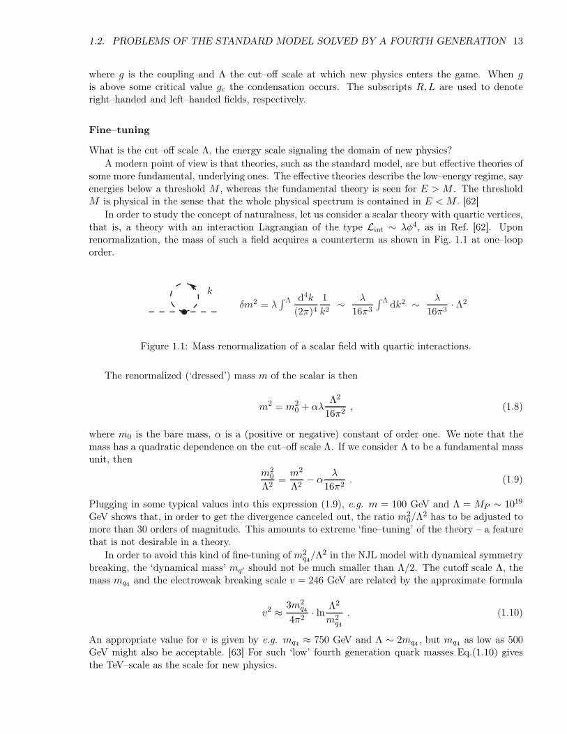
In order to study the concept of naturalness, let us consider a scalar theory with quartic vertices,that is, a theory with an interaction Lagrangian of the type Lint ∼ λφ4, as in Ref. [62]. Uponrenormalization, the mass of such a field acquires a counterterm as shown in Fig. 1.1 at one–looporder.
k
δm2 = λ∫ Λ d4k
(2π)41
k2∼ λ
16π3∫ Λ
dk2 ∼ λ
16π3· Λ2
Figure 1.1: Mass renormalization of a scalar field with quartic interactions.
The renormalized (‘dressed’) mass m of the scalar is then
m2 = m20 + αλ
Λ2
16π2, (1.8)
where m0 is the bare mass, α is a (positive or negative) constant of order one. We note that themass has a quadratic dependence on the cut–off scale Λ. If we consider Λ to be a fundamental massunit, then
m20
Λ2=m2
Λ2− α
λ
16π2. (1.9)
Plugging in some typical values into this expression (1.9), e.g. m = 100 GeV and Λ = MP ∼ 1019
GeV shows that, in order to get the divergence canceled out, the ratio m20/Λ
2 has to be adjusted tomore than 30 orders of magnitude. This amounts to extreme ‘fine–tuning’ of the theory – a featurethat is not desirable in a theory.
In order to avoid this kind of fine-tuning of m2q4/Λ
2 in the NJL model with dynamical symmetrybreaking, the ‘dynamical mass’ mq′ should not be much smaller than Λ/2. The cutoff scale Λ, themass mq4 and the electroweak breaking scale v = 246 GeV are related by the approximate formula
v2 ≈3m2
q4
4π2· ln Λ2
m2q4
. (1.10)
An appropriate value for v is given by e.g. mq4 ≈ 750 GeV and Λ ∼ 2mq4 , but mq4 as low as 500GeV might also be acceptable. [63] For such ‘low’ fourth generation quark masses Eq.(1.10) givesthe TeV–scale as the scale for new physics.
14 CHAPTER 1. MOTIVATION
1.2.2 Flavor democracy – a solution to the naturalness problem
The flavor democracy hypothesis or the democratic mass matrix model was proposed [64] morethan thirty years ago as a solution to some of the problems of the standard model. For threeSM families this approach leads to a number of ‘false’ predictions, such as a low mass for the t–quark [65], but in the case of four families flavor democracy seems fitting since it gives three exactlymassless neutrinos and a heavy neutrino without requiring a large hierarchy among the Yukawacouplings of the fermions of different types [66]. This is the foundation of the hypothesis: the ideathat all fermions of a particular type have equal Yukawa couplings with the Higgs field before thediagonalization of the mass matrix. The three exactly massless neutrinos obtain small masses fromthe slight breaking of democracy.
In order to familiarize ourselves with the ideas of flavor democracy let us consider three differentbases [66, 65]:
− standard Model basis f0 ,
− mass basis fm and
− weak basis fW.In the three family SM quarks are grouped into the following multiplets before symmetry breaking:
u0L
d0L
, u0R , d0R ;
c0L
s0L
, c0R , s0R ;
t0L
b0L
, t0R , b0R . (1.11)
For one family all bases are equal and the Yukawa interaction of, for example, the d–quark massreads
L(d)Y = λd(uL dL)
(φ+
φ0
)dR + h.c. , (1.12)
where λd is the Yukawa coupling and (φ+, φ0)T is the SM Higgs doublet where only the second,neutral component φ0 has a nonzero vacuum expectation value
⟨φ0⟩0= v = 246 GeV (the Higgs
mechanism will be discussed later on, in Section 2.3). The interaction (1.12) leads to a mass termfor the d–quark :
L(d)m = mddd , (1.13)
with md = λd · v/√2.
For n generations the Yukawa couplings form an n× n matrix λij and the Yukawa-term in theSM Lagrangian is a sum over all the flavors. For the down–type quark this interaction reads :
L(d)Y =
n∑
i,j=1
λdij(u0Li d
0Li)
(φ+
φ0
)d0Ri + h.c. , (1.14)
where the quark fields are in the SM basis. Eq. (1.14) gives the mass terms
L(d)m =
n∑
i,j=1
mdij d
0i d
0j , (1.15)
where d1 = d, d2 = s etc and mdij = λdijv/
√2. As will be discussed further on, a bi-unitary
transformation diagonalizes the mass matrix of a given type of fermions and makes the transitionfrom the SM basis to the mass basis.
1.2. PROBLEMS OF THE STANDARD MODEL SOLVED BY A FOURTH GENERATION 15
The basic idea of flavor democracy is that the mass matrix M is fully ‘democratic’ inthe sense that all of its entries have the same value Mij = λv/
√2 ∀ i, j. Such a matrix has two
eigenvalues: a three-fold degenerate eigenvalue Λ1 = 0 and the nonzero Λ2 = 4. For the generic caseof n generations one gets an n× n mass matrix Mf instead of the 4× 4 of SM4. The superscript frefers to the type of fermion considered (up, down, charged lepton, neutrino).
If the model has approximate flavor democracy among the Yukawa couplings then Mf
can be written in terms of the fully democratic matrix described above and a small, democracy-breaking term λM ′
f as [66]
Mf = Y f (M0 + λM ′f ) , (1.16)
where Y f is interpreted as the common Yukawa coupling of fermions of type f and the parameter λis introduced for bookkeeping purposes (as is usually done in perturbative quantum mechanics). λ isassumed to be real and to take values between 0 and 1. The matrixM ′ has entries O(1), and since thefirst three eigenvalues of the fully democratic mass matrix are zero, M ′ gives the first three generationparticles their ‘small’ masses – the deviation of the model from perfect democracy [67, 68, 44].
Again, in the generic case of n generations the first n−1 eigenvalues of M are equal to zero whileone is equal to n so a large hierarchy among the masses of a given species f does not necessarilyrequire a similar hierarchy among the elements of the mass matrix [66, 65].
In order to be able to work with the flavor democracy hypothesis one needs to makethe following assumptions [65]:
1. Before spontaneous symmetry breaking all fermions with the same quantum numbers areindistinguishable so the Yukawa couplings within each type of fermions should be equal:
λdij ≃ λd , λuij ≃ λu , λℓij ≃ λℓ and λνij ≃ λν . (1.17)
This assumption leads to n−1massless particles and one massive particle with mf = n·λfv/√2
for n generations and f = u, d, ℓ, ν.
2. Because there is only one Higgs doublet giving Dirac masses to all four types of fermions itwould seem natural that the Yukawa couplings of different types of fermions be nearly equal:
λd ≃ λu ≃ λℓ ≃ λν . (1.18)
3. A natural value for λ is the SU(2) gauge coupling constant gW . If this were true thenm4 = 2
√2gW v ≈ 450 GeV. On the other hand, if λ = 1 then m4 ≈ 700 GeV, which is close to
the upper limit posed on quark masses by partial wave unitarity (discussed in Section 1.3).
A prediction of the first and second assumptions is that, taking into account the actual massesof the third SM family, namely mντ ≪ mτ < mb ≪ mt, the fourth SM family should exist [65].
1.2.3 Electroweak Precision Data
During the last two decades precision tests have been made at CERN, Fermilab and SLAC. Theresults have provided increasingly precise tests of the SM, so that the SM is now confirmed at at thelevel of virtual quantum effects. The tests also probe the mass scale of the Higgs boson. Even thoughin many cases the agreement between experiment and theory is excellent, there are some observablesof the electroweak precision data (EWPD) that have some tension with the SM predictions. These
16 CHAPTER 1. MOTIVATION
discrepancies may be due to various errors in the measurements, or possibly signals of new physicsbeyond the standard model. Interestingly, it seems that the adding of a fourth generation mightamount to a better agreement with the data. The situation is, however, far from clear.
B physics
Measurements of the b–quark CP–asymmetries, often called B-CP asymmetries have shown severalindications of new physics. During the last years the amount of available data has accumulatedand at the same time the accuracy of some important theoretical calculations has improved. Thesedevelopments make it increasingly apparent that several of the results are difficult to reconcile withSM3 (see e.g. [47, 69, 70, 71]) and provide a test for models going beyond the SM (BSM models).
The problem of the B−CP asymmetries from a phenomenological point of view is that the CKMpicture of CP–violation does not explain all of the experimentally observed phenomena. As will bediscussed later on, in the SM CP-violation is encoded in a few CP violating phases of the quarkmixing matrix, called the CKM matrix. Phenomena not explained by the CKM model are [72] (seeAppendix A for explanations of the parameters) 1:
1. The large difference in direct CP asymmetries is difficult in the SM framework: the direct CPasymmetry is measured to be [75]
∆ACP = ACP (B− → K−π0)−ACP (B
0 → K−π+) = (14.4 ± 2.9)% . (1.20)
Naively this quantity would be expected to vanish but on the other hand it is difficult todraw any conclusions from the value (1.20), since the associated hadronic decays are not fullyunderstood.
2. The need for a non-standard CP-phase has recently been brought up [76, 77] in the study ofBs → ψφ by CDF [78] and D/0 [79] at Fermilab.
Some of the above anomalies may be explained by a fourth generation. The heavyup–type quark of the fourth generation generate a new source of electroweak penguin contributionsince the amplitudes do not obey the decoupling theorem and hence grow as m2
t′ . This might helpto explain two of the anomalies in b→ s transitions and this also helps in explaining the differencein CP asymmetries ∆ACP. [72]
Z-pole anomaly
In addition to the above listed discrepancies in B physics there is a Z-pole observable with a largeanomaly that has been mentioned in the literature [69]: the Z → bb front-back asymmetry Abb
FB
(A.3), which differs by about 3σ from the SM prediction (3.2σ at 99.9% C.L. in 2011 [80], 2.8σ in2006 [81]).
This deviation could be a signal for new physics but there are a few issues that suggest cau-tion [69]:
1 A few years ago there was another parameter that would have been added to this listing; namely the sin 2βparameter (see Eq. (A.2)). In 2008 the SM prediction was approximately 2 − 3 σ larger than the directly measuredvalue (see e.g. [71]). Recent measurements have shifted the parameter towards the SM prediction, and the discrepancyhas vanished. In 2012 the PDG [59] reported the result [73]
β = 0.07+0.06−0.08 , (1.19)
of the HFAG collaboration, which is in agreement with the SM prediction β = 0.018 ± 0.001 [74].
1.3. UNITARITY CONSTRAINTS ON THE FOURTH GENERATION 17
1. the direct determination of Ab (A.5) from the front-back left-right asymmetry ALRFB (A.4),with a deviation of only 0.7σ is consistent with the SM but when Ab is determined fromAb = 4Ab
FB/3Aℓ, with Aℓ the leptonic asymmetry, disagrees by 3.5σ at 99.95% C.L,
2. there is no hint of an Rb anomaly to match the Ab one, so fine-tuning of the left and right-handed Zbb couplings is required as well as an extremely large shift in the right-handedcoupling,
3. Z → bb measurements are known to be difficult.
Another thing to keep in mind is that the deviation could be due to a statistical fluctuation orsubtle systematic error. If the explanation were systematic error Ab
FB should be omitted from theSM fit. In this case the global fit, which is poor with Ab
FB included, becomes excellent, but at thesame time the predicted value of mH gets low values in direct conflict with the search limit 114.4GeV (95% C.L.) [82].
The effective leptonic mixing angle xℓW = sin2 θℓW , extracted from the hadronic asym-metry measurements Ac
FB and QFB agrees with xℓW extracted from AbFB but deviates from the
SM fit (the leptons do not mix in the SM, as we will see). When all measurements are combined,they differ from the SM fit at 99.5% but on the other hand these are the only measurements thatraise the predicted value of mH toward the range required by the search limit. It follows that thedata favors new physics whether the Ab
FB anomaly is genuine or not. In any case an important con-sequence is that the evidence from the SM fit favoring a light Higgs boson becomes less credible. [69]
1.3 Unitarity constraints on the fourth generation
At the quantum level conservation of probability is guaranteed by the unitarity of the scatteringmatrix S, which is generally written as S = 1+ iT with T the matrix describing the interactions ofthe system. The expression for T can be deduced from a given Lagrangian, and its eigenvalues giveinformation about the spectrum of fermion masses. More specifically, the largest eigenvalue of T isused to compute the lowest ‘critical’ value of the mass of fermions. The expression ‘critical mass’is used here to signify the value of mass (mf )crit beyond which the electroweak interactions are nolonger weak, but strong, signaling the breakdown of perturbation theory (the perturbative regimeholds for fermions with mass mf . (mf )crit). At the energy scale of a possible fourth generation thecolor interactions usually denoted as ‘strong interactions’ may actually be weak compared to theelectroweak interactions, due to the asymptotic freedom of QCD. Hence it is conceivable that weakinteractions dominate at the scale of fourth generation masses and that these new particles maybe bound together by the SU(2) × U(1) gauge bosons, giving ‘quarkonia’ and ‘leptonia’ bound byW, Z, H. The long–distance behavior of these states would nevertheless be explained by QCD, sincethe color interactions are known to become strong at small energies, but since the small–distance(high–energy) behavior is dominantly described by the electroweak interactions, these are the onesto study when investigating the validity of perturbation theory, the series expansion in powers ofthe coupling. Perturbation theory is applicable as long as terms of high orders are subleading anddo not overtake the lower–order ones. [83]
A tool used to study unitarity is called ‘partial wave analysis’ – a method which we shall nowbriefly review. This method can be used to bound the masses of a possible fourth generation. Ithas also been used to deduce an upper limit on the Higgs boson mass [84].

18 CHAPTER 1. MOTIVATION
Partial wave analysis
A generic scattering amplitude A may be written in terms of ‘partial waves’ :
A = 16π∞∑
ℓ=0
(2ℓ+ 1)Pℓ(cos θ)aℓ , (1.21)
where the Pℓ(cos θ) are Legendre polynomials and aℓ gives the spin–ℓ partial wave (see e.g. [85]).We recall that the differential cross section of a 2 → 2 scattering is simply
dσ
dΩ=
1
64π2s|A|2 , (1.22)
which, together with equation (1.21) gives the total cross section
σ =8π
s
∞∑
ℓ,ℓ′=0
(2ℓ+ 1)(2ℓ′ + 1)aℓaℓ′
∫ +1
−1d cos θPℓ(cos θ)Pℓ′(cos θ) (1.23)
=16π
s
∞∑
ℓ=0
(2ℓ+ 1)|aℓ|2 , (1.24)
where, going from (1.23) to (1.24) the orthogonality property of the Legendre polynomials has beenused. We note that the cross section of Eq. (1.24) is a sum of positive definite terms. On theother hand, by the optical theorem, the cross section is proportional to the imaginary part of theamplitude in the θ = 0 direction :
σ =1
sℑ [A(θ = 0)] , (1.25)
which together with (1.24) gives
|aℓ|2 = ℑ(aℓ) =⇒ [ℜ(aℓ)]2 +[ℑ(aℓ)−
1
2
]2=
1
4, (1.26)
which is nothing but the equation for a circle of radius1
2– the ‘unitarity circle’ – centered at (0,
1
2)
in the complex aℓ plane. The real part of the partial wave aℓ lies thus in the region
ℜ(aℓ) <1
2∀ℓ . (1.27)
Limits on fermion masses
In the high–energy limit√s≫ mf the amplitudes of 2 → 2 processes simplify, and since this is also
the case of current experiments (notably at the LHC) this is the limit upon which we focus. In thishigh-energy limit the tree–level amplitudes of certain 2 → 2 processes, such as [86]
f f −→ f f , W+W−, ZZ, ZH, HH (1.28)
tend toward the constant value of GFm2f . When mf is very large the constant GFm
2f may become
of the order of unity, signaling the saturation of the tree–level unitarity of the S–matrix. Whenthe S–matrix is saturated already at tree level, this implies that the higher–order corrections needto be relatively large, which in turn implies that the coupling is relatively strong and that one isworking at the limit of the validity of perturbation theory.
1.3. UNITARITY CONSTRAINTS ON THE FOURTH GENERATION 19
This is also seen from the point of view of partial–wave analysis. As noted above, the moststringent bound on the mass of new fermions is given by the largest eigenvalue of the T matrix. Inthe partial wave analysis presented above, the ℓ = 0 partial wave is computed from
a0 =1
32π
∫ +1
−1d cos θT . (1.29)
For quarks (leptons) the smallest critical mass comes from the spin–0 (spin–1) matrix, giving thefollowing tree–level results [83]
mq <4√2 · πGF
1
5 + sin2 θC× 1
Nand (1.30)
mℓ <4√2 · πGF
1
1 + sin2 θC× 1
N, (1.31)
when the particles of a doublet are assumed degenerate: m1 = m2 = m with m1, m2 the masses ofthe particles of an SU(2) doublet. Here GF is the Fermi constant, θC is the Cabibbo angle and Nis the number of nearly degenerate doublets, ‘nearly degenerate’ meaning that the mass differenceof the particles in a given doublet is much smaller than the masses themselves. The doublets of thethree–generation SM are not nearly degenerate, so for a degenerate fourth family N = 1. In theabsence of mixing between doublets, i.e. for θ = 0, these limits read :
mq . 550 GeV and mℓ . 1200 GeV . (1.32)

20 CHAPTER 1. MOTIVATION
Chapter 2
The Standard Model
The standard model of elementary particle physics is a gauge theory – a theory based upon the lo-cal, continuous symmetries of the system, ‘local’ meaning that the parameters of the transformationdepend on the space–time coordinates. Symmetry transformations have a mathematical descriptionin terms of group theory, and more specifically continuous symmetries are described by Lie groups.Each Lie group has an associated Lie algebra, a vector space over some field and where an operatorcalled the Lie bracket has been defined. The standard model is based upon the symmetry group(the gauge group) SU(3)×SU(2)×U(1), where each group of this direct product is associated witha symmetry of the system. SU(3) is the color group, SU(2) and U(1) the isospin and hyperchargesymmetry groups. The theory of quantum chromodynamics (QCD) [36, 37, 34, 87] is based uponthe gauge group SU(3) whereas the Glashow–Weinberg–Salam (GWS) [46, 31, 28, 22] theory ofelectroweak interactions is based on SU(2)× U(1). The SU(2)×U(1) symmetry is broken sponta-neously by the presence of a scalar field, separating the interactions into weak and electromagneticones. This spontaneous symmetry breaking (SSB) generating masses for the standard model par-ticles is called the Higgs mechanism [88, 89, 90] and the associated scalar field is called the Higgsfield.
In the following we give a brief review of the salient features of this theory that in elementaryparticle physics is called the standard model. We start by presenting the theory of strong interactionsbefore going on to the electroweak theory and the breaking of the SU(2)×U(1) symmetry and thegeneration of mass.
2.1 Quantum chromodynamics
The theory that describes the strong interactions that bind together nuclear matter is called quantumchromodynamics (QCD) – from the Greek word ‘chromo’ meaning color. The gauge group SU(3) ofthe theory is often called the ‘color group’, with Nc = 3 the number of colors (the number of degreesof freedom in the fundamental representation) for the case of QCD. The quanta of the gauge field,the ‘gluons’, live in the adjoint representation of the gauge group and hence there are N2
c − 1 = 8of them.
The Lagrangian density of a system must respect the relevant symmetries, for QCD this meansthat the Lagrangian is required to be invariant under SU(3). The Yang–Mills Lagrangian for anon-abelian theory with the Dirac field ψ reads
LQCD = LDirac + LYM = ψ(i /D −m)ψ −GaµµGaµν , (2.1)
21

22 CHAPTER 2. THE STANDARD MODEL
where Gaµν is the field strength tensor
Gaµν = ∂µA
aν − ∂νA
aµ + gfabcAb
µAcν , (2.2)
with Aaµ the gauge field with color index a and Lorentz index µ and g is a constant that is eventually
identified with the gauge coupling. The fabc are the (completely antisymmetric) structure constantsof the SU(3) algebra : [
ta, tb]= ifabctc . (2.3)
The ta are the generators of the algebra.The notation can be abbreviated writing
Gµ ≡ Gaµt
a and Aµ ≡ Aaµt
a , (2.4)
where summation over a is implied.A specific representation of the group is given by the Gell-Mann matrices λa ≡ ta/2, after the
Nobel–prize winning physicist Murray Gell–Mann. The action of the covariant derivative Dµ on ψin (2.1) reads
Dµψ(x) = [∂µ − igAµ(x)]ψ(x) , (2.5)
where we have used the Feynman slash notation
/D ≡ γµDµ , (2.6)
for γµ generators of the Clifford algebra in four dimensions. Matter fields transform in the fundamen-tal representation whereas gauge fields transform in the adjoint (antifundamental) representation.
From the Lagrangian (2.1) and the identities (2.2), (2.4), (2.3) we see that invariance underSU(3) implies that the spinors ψ transform as (see e.g. [91])
ψ(x) → V (x)ψ(x) , (2.7)
where V (x) = eigtaαa(x), αa(x) being a space–time dependent vector whose ath component is mul-
tiplied by the corresponding Lie algebra generator. The gauge field transforms as
Aµ → V (x)
(Aµ +
i
g∂µ
)V †(x) . (2.8)
2.1.1 Gauge fixing and Faddeev–Popov ghosts
Let us for a moment discuss the quantization of a non–abelian field theory in the path integralformalism.
The generating functional of a QFT with a Yang–Mills Lagrangian LYM ≡ LYM (Aaµ) =
−1
4(F a
µν)2 is written as a functional integral over the gauge field Aa
µ
Z ∼∫
DA exp
(i
∫d4x L
)(2.9)
∼∫
DA eiS[Aaµ] , (2.10)
up to a normalization factor. Here the action S is
S[Aa
µ
]≡∫
dtL(Aaµ) =
∫dtd3xL(Aa
µ) , (2.11)
2.1. QUANTUM CHROMODYNAMICS 23
with L the spatial integral of the Lagrangian density L. Since L is invariant under a (non–abelian)gauge transformation, and gauge transformations are continuous, there is an infinite number ofdirections in configuration space along which the Lagrangian is unchanged. The choice of directionin configuration space – the gauge choice – should not affect the physics of the system, so these‘redundant’ degrees of freedom corresponding to the different gauges need to be integrated out of(2.11), since the dynamics is given by the action (or the Lagrangian) through the equations ofmotion. This procedure of choosing direction in phase space is often called gauge fixing.
A clever way to fix the gauge, proposed by Faddeev and Popov [92], is to insert the identity indisguise into the functional integral (2.10)
1 =
∫Dα(x) δ (G(A)) det
(δG(Aα)
δα
). (2.12)
This equation enforces a gauge–fixing condition G(A) = 0 at every spacetime point x. In (2.12) Aα
is the gauge field transformed by a finite gauge transformation
Aαµ ≡ (Aα)aµt
a = eiαata(Ab
µtb +
i
g∂µ
)e−iαctc , (2.13)
with the ta generators of the adjoint representation of SU(3), satisfying
(tb)ac = ifabc . (2.14)
For the determinant in (2.12) it is convenient to write (2.13) in its infinitesimal form
(Aα)aµ = Aaµ +
1
g∂µα
a + fabcAbµα
c (2.15)
= Aaµ +
1
gDµα
a , (2.16)
where one recognizes the covariant derivative Dµ of (2.5) using (2.14). When the generalized Lorentzgauge condition G(A) = ∂µAa
µ(x)−ωa(x), with ωa(x) a Gaussian weight, is chosen the result (2.16)gives
δG(Aα)
δα=
1
g∂µDµ (2.17)
The idea of Faddeev and Popov was to write the determinant of the left–hand side of (2.17)as a functional integral over Grassmannian (i.e. fermionic or anticommuting) fields c, c, with aGaussian integrand
det
(1
g∂µDµ
)=
∫DcDc exp
[i
∫d4x c(−∂µDµ)c
]. (2.18)
The fields c, c that appear in this way are called Faddeev–Popov ghosts or simply ghosts.The ghosts couple to the gauge field through the minimal coupling of the covariant derivativecAµc ∈ cDµc, giving vertices with one external gauge boson and two ghosts. These ghost fields arenot physical since they have no asymptotic states. They arise, however, as intermediate states inloop calculations. They are crucial to getting results that are gauge invariant and need to be takeninto account when renormalizing QCD.
24 CHAPTER 2. THE STANDARD MODEL
2.1.2 Renormalization and asymptotic freedom
Non–abelian gauge theories have a very interesting characteristic, which is not present in the Abeliancase. It turns out that at very high energies the strength of the color interactions, as given by theQCD coupling αs, become weak. This property is called asymptotic freedom [35, 37, 36, 34, 33],signaling the asymptotic tendency
asymptotic freedom : αs(µ2) ≪ 1 when µ2 ≫ Λ2
QCD , (2.19)
with ΛQCD ≃ 200 MeV the QCD ‘cut-off scale’. The coupling αs is related to the gauge coupling gthrough
αs ≡g2
4π. (2.20)
The property (2.19) is extracted from the dependence of the coupling on the energy scale atwhich it is determined. Actually, the physics of a system quite generally depends on the scale atwhich one studies it. For instance, at the low energies in the domain of application of Newtonianmechanics, the orbit of the Earth may at the lowest order be computed by approximating the motionof the Earth around the sun as a classical two–body problem of pointlike particles. However, when‘zooming in’ a little bit one notices that the sun is not pointlike at all, and at this distance scalethe shape and varying density of the sun have to be taken into account. Zooming in yet more onediscerns even details of the Earth, and sees that it is not a pointlike particle either, and that whenwanting to do an even more comprehensive calculation you need to take the finiteness of its sizeinto account, too. [93] (For published notes see e.g. [94] by the same author.)
A similar situation arises in elementary particle physics – the physics of the system dependsupon the energy scale considered. It is well known that some loops diagrams lead to divergences(see e.g. [95]) in quantum field theories. Whenever the divergences come from a finite number ofsubdiagrams they can be ‘absorbed’ into a finite number of so–called counterterms. The procedureof identifying the divergences and grouping them into counterterms is called renormalization. Thisrenders the physical observables finite, since the infinities are canceled by the counterterms. Indoing so, however, one needs to introduce an arbitrary scale µ that is called the renormalizationscale. The finite, renormalized, quantities then depend upon this scale, as does for example thecoupling ‘constant’ αs that is in fact scale–dependent αs ≡ αs(µ
2) and not a constant at all.The dependence of the gauge coupling g on the renormalization scale µ is given by the β–function
(also called the Callan–Symanzik function)
β(g) ≡ ∂g
∂ log(µ/µ0), (2.21)
when the coupling is known at some reference scale µ0. For non–abelian theories the generalexpression at the leading order in perturbation theory reads (see e.g. [96])
β(g) = − g3
(4π)3
(11
3C
(A)2 − 4
3nfC
(r)
)+O(g5) , (2.22)
where C(A)2 is the quadratic Casimir operator for the adjoint representation, C(r) is the Casimir
operator for the representation r and nf is the species of fermions. When the gauge group isSU(N) these are, for the fundamental (F ) and adjoint (A) representations
C(F )(N) =1
2, C
(F )2 =
N2 − 1
2Nand C(A)(N) = C
(A)2 (N) = N . (2.23)
2.2. LOCAL SU(2) AND U(1) SYMMETRIES 25
For QCD with gauge group SU(3) the β–function (2.22) is negative when the number of fermionspecies is nf ≤ 16, which implies that the number of families can be at most four. Since we believethat QCD indeed does exhibit asymptotic freedom the β–function should be negative, meaningthat the coupling diminishes with the energy, this gives an upper limit on the number of fermiongenerations.
2.2 Local SU(2) and U(1) symmetries
Besides the theory of strong interactions just covered, the standard model contains the electroweakinteractions, whose gauge group is SU(2) × U(1). According to Noether’s theorem [97] to eachsymmetry of a system there is related a conserved current and a conserved charge. The conservedcharges of the electroweak theory [98, 46, 31, 28] are the isospin I for SU(2) [99] and hyperchargeY for U(1) – one often sees the notation SU(2)I × U(1)Y . This SU(2) × U(1) symmetry, is notan invariance of the low–energy theory, because it is broken by another field at what is called theelectroweak scale v ≈ 246 GeV. After this symmetry breaking, the isospin and hypercharge are nolonger conserved separately, but combine to form just one conserved charge, the electric charge. Inother words, the SU(2)I × U(1)Y symmetry group is broken down to a subgroup: U(1)Q.
The field that breaks the electroweak symmetry is called the Higgs field [88, 89, 90]. It is ascalar field whose non–zero vacuum expectation value (VEV) is responsible for the breaking of thesymmetry and the generation of mass of the standard model particles. The quantum associatedwith the field, the Higgs boson seems to have been found at the time of writing this report [100, 101].
2.2.1 Isospin symmetry
As already noted in Section 1.2.1, the particles of the standard model come in doublets. A generalfermion doublet Ψ(x) is of the form Ψ(x) = (ψ1(x), ψ2(x))
T , with ψ1, ψ2 complex fields. Underthe SU(2) isospin symmetry group such a doublet transforms as (see e.g. [102])
Ψ(x) → Ψ′(x) = e−iαa(x)taΨ(x) , (2.24)
where the ta are generators of SU(2) and the parameters αa(x) are local. The Pauli matrices σa
give a specific representation of the group such that ta = σa/2. In order for the Dirac Lagrangian
LDirac = ψ(x) (iγµ∂µ −m)ψ(x) (2.25)
to be invariant under the transformation (2.24), the partial derivative ∂µ must be replaced by thecovariant derivative Dµ, given in (2.5). The covariant derivative transforms as the Dirac field (thisis the meaning of a ‘covariant’ derivative)
(DµΨ(x))′ = e−iαa(x)taDµΨ(x) , (2.26)
so the gauge field should transform as
A′aµ t
a = U(α)Aaµt
aU−1(α)− i
g[∂µU(α)]U−1(α) , (2.27)
where U(α) = exp (−iαa(x)ta).Now we are ready to add the Yang–Mills term for the gauge field to get the complete Lagrangian
L = LYM + LDirac = −1
2Tr(FµνFµν) + ψ(x) (iγµDµ −m)ψ(x) , (2.28)
where we see interactions between the matter fields and the gauge bosons appearing from theminimal coupling in the covariant derivative.

26 CHAPTER 2. THE STANDARD MODEL
2.2.2 Quantum electrodynamics
After the breaking of the SU(2)I ×U(1)Y symmetry of the electroweak theory the remaining invari-ant subgroup is U(1). This is however not the same U(1) group as the original one; originally, theU(1)Y symmetry has the associated quantum number that is the hypercharge, whereas the relevantquantum number after the breaking is the electric charge so the one may use the notation U(1)Q.The electric charge Q is in fact a linear combination of the quantum numbers of the two brokensymmetries, namely
Q = I3 +Y
2, (2.29)
with I3 the third generator of the SU(2) isospin algebra[Ii, Ij
]= iǫijkIk (the structure constants
of SU(2) are the components of the completely antisymmetric tensor with three indices).The remaining U(1)Q group gives rise to an Abelian gauge theory called Quantum electrody-
namics (QED), describing the electric and magnetic interactions of matter. It may be derived fromthe free Dirac equation, as done above for the SU(2) gauge theory, simply by replacing the partialderivative in the Dirac term with a covariant one and by also inserting a Yang–Mills term for thegauge field into the Lagrangian. The only difference to the treatment of Eqs. (2.24)–(2.28) is thatsince QED is based on an Abelian gauge group, there is no commutator algebra for the generators(the generators commute) and the transformation matrix that is called U(α) in (2.27) simplifies
UQED(α) = exp (−iα(x)) . (2.30)
The vector αa(x) is now just one real parameter α, reflecting the fact that only one degree of freedomis enough to uniquely determine U(1) transformations. The associated Lagrangian reads
LQED = LDirac + Lγ (2.31)
= ψ(x) (iγµDµ −m)ψ(x) − 1
4FµνFµν (2.32)
= −1
4FµνFµν + ψ(x) (iγµ∂µ −m)ψ(x) − eψ(x)γµψ(x)A
µ(x) , (2.33)
where, in going from (2.31) to (2.32) Eqs. (2.25),(2.28) have been used as has the definition of thecovariant derivative (2.5) in the last equality. The covariant derivative (2.5) simplifies for an Abeliantheory:
Dµψ(x) = (∂µ + ieAµ)ψ , (2.34)
where the parameter α = α(x) of (2.5) actually is the electric charge e (e 6= e(x)), appearing in(2.33) (we have written e instead of Q, as is often done). An important thing to note about theLagrangian (2.33) is that a mass term for the gauge field Aµ is missing. This is so because sucha term would break the gauge symmetry and is thus forbidden. The last term in (2.33) gives thecoupling of the electromagnetic field to matter. It arises from the minimal coupling of the covariantderivative and may also be written as a current Jµ coupling to the gauge field Aµ
eψ(x)γµψ(x)Aµ(x) ≡ Jµ(x)A
µ(x) , (2.35)
with Jµ the Noether current [97].
2.3 Spontaneous symmetry breaking
As long as the SU(2) and U(1) gauge theories presented in the previous section 2.2 do not includemass terms
∼ m2AA
µAµ (2.36)
2.3. SPONTANEOUS SYMMETRY BREAKING 27
for the gauge mediators the theories work well: they are gauge invariant and renormalizable but assoon as one attempts to introduce conventional mass terms for the gauge bosons the theory losesthese characteristics. Experimentally, however, it is known that some of the gauge bosons observedin nature are indeed massive, so there has to be some other means of mass generation besides thead hoc addition of terms like (2.36).
The Goldstone model reviewed in Appendix B provides such a means of mass generation, throughthe appearance of massless bosons that can be interpreted as longitudinal degrees of freedom of thegauge fields. The Goldstone model is the basis for another model where spontaneous symmetrybreaking appears – the Higgs model, a field theory which is invariant under U(1) gauge transforma-tions. The ‘Higgs field’ of this model breaks the SU(2)I × U(1)Y symmetry of the combined weakand electromagnetic interactions of the electroweak theory down to the remaining U(1)Q of QED.
2.3.1 The Higgs mechanism
The Goldstone theorem (see the Appendices, B) is evaded in gauge theories since the proof of thetheorem requires all of the usual axioms of quantum field theory to be valid: manifest Lorentzcovariance, positivity of norms and so on. This is a problem because there is no possible gauge-fixing condition for which a given gauge theory would obey all of the axioms of usual field theories.For example: in covariant gauges states of negative norm (longitudinal photons) arise whereas inaxial gauges Lorentz covariance is not manifest. As it turns out, both of these problems are solvedin the physical spectrum of the theory, where massive vector particles arise without ruining therenormalizability of the theory, as first suggested by Anderson [103, 104]. Englert and Brout [90]and independently Higgs [89, 105] carried out the generalization to relativistic fields. Finally, therenormalizability of gauge field theories in the presence of spontaneous symmetry breaking wasshown by ’t Hooft [30].
Abelian case
The Higgs model is a field theory invariant under U(1) gauge transformations, obtained from theGoldstone model (see Appendix B) by replacing the partial derivatives by covariant ones (2.34) andintroducing a Yang-Mills term FµνF
µν into (B.8) :
L = (Dµφ)†(Dµφ)− µ2φ†φ− λ(φ†φ)2 − 1
4FµνF
µν , (2.37)
with φ the ‘Higgs field’. The ground state of the system corresponds to a minimum of the ‘potential’
V (φ) = µ2φ†φ+ λ(φ†φ)2
= µ2|φ|2 + λ|φ|4 . (2.38)
For λ > 0, which is required for V to have a minimum, two situations arise. For µ2 > 0 the origin|φ|2 = 0 is the point where the state of lowest energy is obtained; here both φ(x) and Aµ(x) vanish.The ground state is clearly invariant (under the gauge group U(1)) and is unique. If, on the otherhand, µ2 < 0 then the potential has the form of a ‘mexican hat’ whose minimum is at
|φ| =√
−µ2
2λ≡ v√
2. (2.39)
The vacuum is now given by any of the points on the ring of radius v/√2 in the complex φ–plane.
(The numerical value of v is ∼ 246 GeV in the SM.)
28 CHAPTER 2. THE STANDARD MODEL
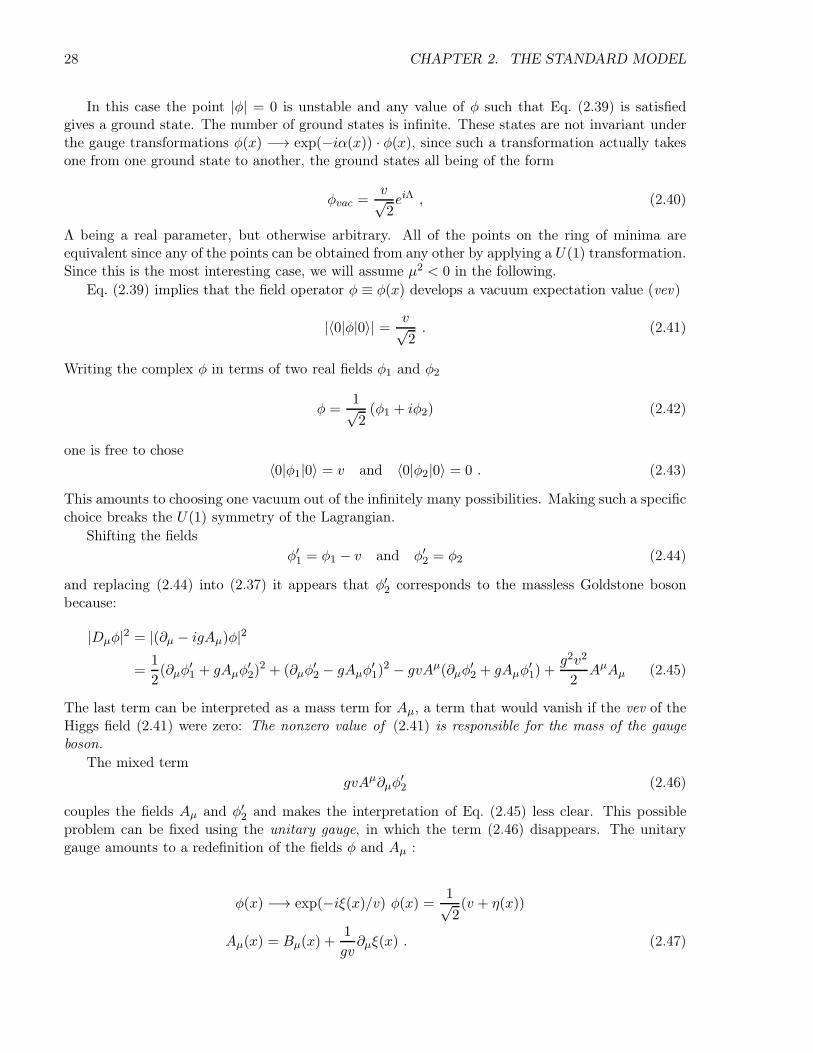
In this case the point |φ| = 0 is unstable and any value of φ such that Eq. (2.39) is satisfiedgives a ground state. The number of ground states is infinite. These states are not invariant underthe gauge transformations φ(x) −→ exp(−iα(x)) · φ(x), since such a transformation actually takesone from one ground state to another, the ground states all being of the form
φvac =v√2eiΛ , (2.40)
Λ being a real parameter, but otherwise arbitrary. All of the points on the ring of minima areequivalent since any of the points can be obtained from any other by applying a U(1) transformation.Since this is the most interesting case, we will assume µ2 < 0 in the following.
Eq. (2.39) implies that the field operator φ ≡ φ(x) develops a vacuum expectation value (vev)
|〈0|φ|0〉| = v√2. (2.41)
Writing the complex φ in terms of two real fields φ1 and φ2
φ =1√2(φ1 + iφ2) (2.42)
one is free to chose
〈0|φ1|0〉 = v and 〈0|φ2|0〉 = 0 . (2.43)
This amounts to choosing one vacuum out of the infinitely many possibilities. Making such a specificchoice breaks the U(1) symmetry of the Lagrangian.
Shifting the fields
φ′1 = φ1 − v and φ′2 = φ2 (2.44)
and replacing (2.44) into (2.37) it appears that φ′2 corresponds to the massless Goldstone bosonbecause:
|Dµφ|2 = |(∂µ − igAµ)φ|2
=1
2(∂µφ
′1 + gAµφ
′2)
2 + (∂µφ′2 − gAµφ
′1)
2 − gvAµ(∂µφ′2 + gAµφ
′1) +
g2v2
2AµAµ (2.45)
The last term can be interpreted as a mass term for Aµ, a term that would vanish if the vev of theHiggs field (2.41) were zero: The nonzero value of (2.41) is responsible for the mass of the gaugeboson.
The mixed term
gvAµ∂µφ′2 (2.46)
couples the fields Aµ and φ′2 and makes the interpretation of Eq. (2.45) less clear. This possibleproblem can be fixed using the unitary gauge, in which the term (2.46) disappears. The unitarygauge amounts to a redefinition of the fields φ and Aµ :
φ(x) −→ exp(−iξ(x)/v) φ(x) = 1√2(v + η(x))
Aµ(x) = Bµ(x) +1
gv∂µξ(x) . (2.47)
2.4. THE GLASHOW–WEINBERG–SALAM MODEL 29
Now the Lagrangian (2.37) may be written
L =1
2[∂µη − igBµ(v + η)]2 − µ2
2(v + η)2 − λ
4(v + η)4 − 1
4(∂µBν − ∂νBµ)
2
= L0 + L1 , (2.48)
with L0 the free Lagrangian density for a massive vector field Bµ with mass M = gv and a scalarmeson η with mass m =
√2µ and
L1 =1
2g2BµB
µη(2v + η)− λv2η3 − 1
4λη4 (2.49)
the interaction Lagrangian. The would-be-Goldstone boson ξ(x) has disappeared from the La-grangian and the massless gauge field Aµ and the scalar field ξ have combined to form a massivevector field Bµ.
Non-abelian case
The generalization of the above mechanism to a case with a non-Abelian gauge field is straightfor-ward. In the Lagrangian (2.37) one just uses the covariant derivative (2.5) instead of (2.34) and thefield strength tensor (2.2).
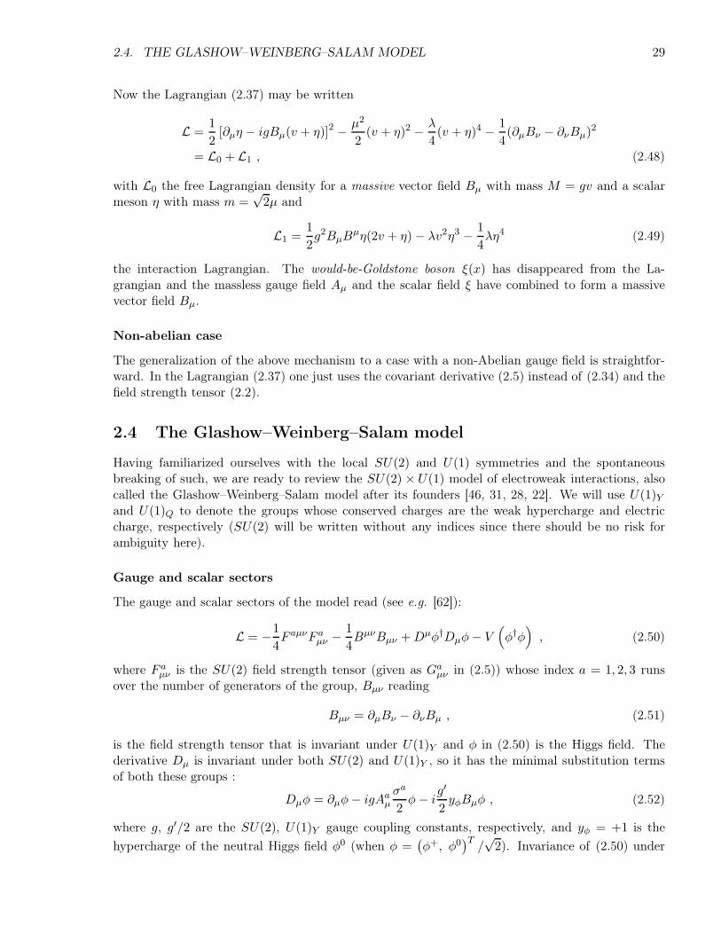
2.4 The Glashow–Weinberg–Salam model
Having familiarized ourselves with the local SU(2) and U(1) symmetries and the spontaneousbreaking of such, we are ready to review the SU(2) × U(1) model of electroweak interactions, alsocalled the Glashow–Weinberg–Salam model after its founders [46, 31, 28, 22]. We will use U(1)Yand U(1)Q to denote the groups whose conserved charges are the weak hypercharge and electriccharge, respectively (SU(2) will be written without any indices since there should be no risk forambiguity here).
Gauge and scalar sectors
The gauge and scalar sectors of the model read (see e.g. [62]):
L = −1
4F aµνF a
µν −1
4BµνBµν +Dµφ†Dµφ− V
(φ†φ), (2.50)
where F aµν is the SU(2) field strength tensor (given as Ga
µν in (2.5)) whose index a = 1, 2, 3 runsover the number of generators of the group, Bµν reading
Bµν = ∂µBν − ∂νBµ , (2.51)
is the field strength tensor that is invariant under U(1)Y and φ in (2.50) is the Higgs field. Thederivative Dµ is invariant under both SU(2) and U(1)Y , so it has the minimal substitution termsof both these groups :
Dµφ = ∂µφ− igAaµ
σa
2φ− i
g′
2yφBµφ , (2.52)
where g, g′/2 are the SU(2), U(1)Y gauge coupling constants, respectively, and yφ = +1 is the
hypercharge of the neutral Higgs field φ0 (when φ =(φ+, φ0
)T/√2). Invariance of (2.50) under

30 CHAPTER 2. THE STANDARD MODEL
SU(2)× U(1)Y gives the infinitesimal transformations of the fields :
δAaµ = −1
g∂µα
a + εabcαbAbµ ,
δBµ = −2
g∂µβ ,
δφ = −iαaσa
2φ− iyφβφ , (2.53)
where αa (a = 1, 2, 3), β are the parameters of the SU(2), U(1)Y transformations. (The choiceα1 = α2 = 0 and α3 = 2β = θ corresponds to the QED U(1) transformation δφ+ = −iθφ+, δφ0 =0.) Taking the scalar potential (2.38) with µ2 = −m2 the ground state of φ is at
〈φ〉 =(
0v√2
), (2.54)
with v given in (2.39). The gauge field mass matrix is obtained from the matrix of the covariantderivative (2.52), which in the ground state 〈φ〉 reads
〈Dµφ〉 =
−ig v√
2· A1
µ−A2µ
2
+i v√2· gA3
µ−g′Bµ
2
. (2.55)
The masses of the gauge bosons come from the terms quadratic in the gauge field and linear inthe Higgs field, and more precisely, of the vev of this term:
⟨Dµφ†Dµφ
⟩. Computing the matrix
product reveals the mass eigenstates :
W±µ =
A1µ ∓ iA2
µ√2
, MW =1
2gv , (2.56)
Z0µ =
gA3µ − g′Bµ√g2 + g′2
, MZ =1
2
√g2 + g′2v , (2.57)
Aµ =g′A3
µ + gBµ√g2 + g′2
, MA = 0 . (2.58)
Only the photon Aµ is massless after the breaking of the SU(2)×U(1)Y symmetry – the remainingsymmetry group is U(1)Q of QED. Both neutral bosons Aµ and Zµ are superpositions of the samegenerators – they depend on the same basis vectors and the mixing angle between them is calledthe Weinberg angle :
sin θW =g′√
g2 + g′2, cos θW =
g√g2 + g′2
, tan θW =g′
g. (2.59)
Substituting (2.59) into (2.57),(2.58) gives the Z boson and the photon in terms of the generatorsand θW :
Zµ = cos θWA3µ − sin θWBµ , (2.60)
Aµ = sin θWA3µ + cos θWBµ . (2.61)
The masses of the gauge bosons and the Weinberg mixing angle can be grouped together to aparameter traditionally denoted as ρ :
ρ =M2
W
M2Z cos2 θW
, (2.62)
2.5. QUARK AND LEPTON MIXING 31
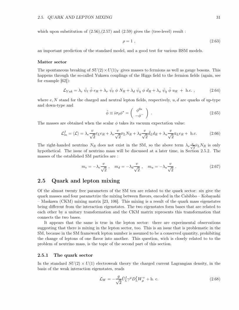
which upon substitution of (2.56),(2.57) and (2.59) gives the (tree-level) result :
ρ = 1 , (2.63)
an important prediction of the standard model, and a good test for various BSM models.
Matter sector
The spontaneous breaking of SU(2)×U(1)Y gives masses to fermions as well as gauge bosons. Thishappens through the so-called Yukawa couplings of the Higgs field to the fermion fields (again, seefor example [62]):
LY uk = λe ψℓ φ eR + λν ψℓ φ NR + λd ψq φ dR + λu ψq φ uR + h.c. , (2.64)
where e,N stand for the charged and neutral lepton fields, respectively, u, d are quarks of up-typeand down-type and
φ ≡ iσ2φ∗ =
(φ0∗
−φ−). (2.65)
The masses are obtained when the scalar φ takes its vacuum expectation value:
Lfm = 〈L〉 = λe
v√2eLeR + λν
v√2νLNR + λd
v√2dLdR + λu
v√2uLeR + h.c. (2.66)
The right-handed neutrino NR does not exist in the SM, so the above term λνv√2νLNR is only
hypothetical. The issue of neutrino mass will be discussed at a later time, in Section 2.5.2. Themasses of the established SM particles are :
me = −λev√2, md = −λd
v√2, mu = −λu
v√2. (2.67)
2.5 Quark and lepton mixing
Of the almost twenty free parameters of the SM ten are related to the quark sector: six give thequark masses and four parametrize the mixing between flavors, encoded in the Cabibbo – Kobayashi– Maskawa (CKM) mixing matrix [23, 106]. This mixing is a result of the quark mass eigenstatesbeing different from the interaction eigenstates. The two eigenstates form bases that are related toeach other by a unitary transformation and the CKM matrix represents this transformation thatconnects the two bases.
It appears that the same is true in the lepton sector: there are experimental observationssuggesting that there is mixing in the lepton sector, too. This is an issue that is problematic in theSM, because in the SM framework lepton number is assumed to be a conserved quantity, prohibitingthe change of leptons of one flavor into another. This question, wich is closely related to to theproblem of neutrino mass, is the topic of the second part of this section.
2.5.1 The quark sector
In the standard SU(2) × U(1) electroweak theory the charged current Lagrangian density, in thebasis of the weak interaction eigenstates, reads
LW = − g√2U ILγ
µDILW
+µ + h. c. (2.68)
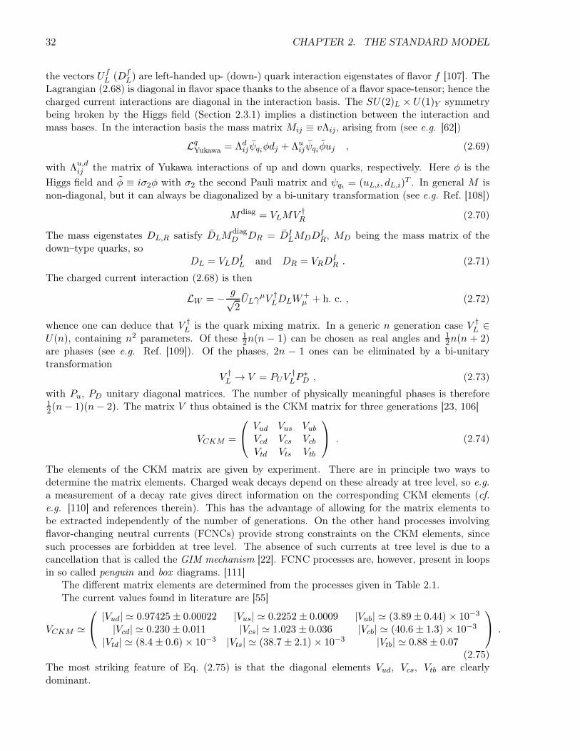
32 CHAPTER 2. THE STANDARD MODEL
the vectors UfL (Df
L) are left-handed up- (down-) quark interaction eigenstates of flavor f [107]. TheLagrangian (2.68) is diagonal in flavor space thanks to the absence of a flavor space-tensor; hence thecharged current interactions are diagonal in the interaction basis. The SU(2)L × U(1)Y symmetrybeing broken by the Higgs field (Section 2.3.1) implies a distinction between the interaction andmass bases. In the interaction basis the mass matrix Mij ≡ vΛij , arising from (see e.g. [62])
LqYukawa = Λd
ijψqiφdj + Λuijψqi φuj , (2.69)
with Λu,dij the matrix of Yukawa interactions of up and down quarks, respectively. Here φ is the
Higgs field and φ ≡ iσ2φ with σ2 the second Pauli matrix and ψqi = (uL,i, dL,i)T . In general M is
non-diagonal, but it can always be diagonalized by a bi-unitary transformation (see e.g. Ref. [108])
Mdiag = VLMV †R (2.70)
The mass eigenstates DL,R satisfy DLMdiagD DR = DI
LMDDIR, MD being the mass matrix of the
down–type quarks, soDL = VLD
IL and DR = VRD
IR . (2.71)
The charged current interaction (2.68) is then
LW = − g√2ULγ
µV †LDLW
+µ + h. c. , (2.72)
whence one can deduce that V †L is the quark mixing matrix. In a generic n generation case V †
L ∈U(n), containing n2 parameters. Of these 1
2n(n − 1) can be chosen as real angles and 12n(n + 2)
are phases (see e.g. Ref. [109]). Of the phases, 2n − 1 ones can be eliminated by a bi-unitarytransformation
V †L → V = PUV
†LP
∗D , (2.73)
with Pu, PD unitary diagonal matrices. The number of physically meaningful phases is therefore12(n− 1)(n − 2). The matrix V thus obtained is the CKM matrix for three generations [23, 106]
VCKM =
Vud Vus VubVcd Vcs VcbVtd Vts Vtb
. (2.74)
The elements of the CKM matrix are given by experiment. There are in principle two ways todetermine the matrix elements. Charged weak decays depend on these already at tree level, so e.g.a measurement of a decay rate gives direct information on the corresponding CKM elements (cf.e.g. [110] and references therein). This has the advantage of allowing for the matrix elements tobe extracted independently of the number of generations. On the other hand processes involvingflavor-changing neutral currents (FCNCs) provide strong constraints on the CKM elements, sincesuch processes are forbidden at tree level. The absence of such currents at tree level is due to acancellation that is called the GIM mechanism [22]. FCNC processes are, however, present in loopsin so called penguin and box diagrams. [111]
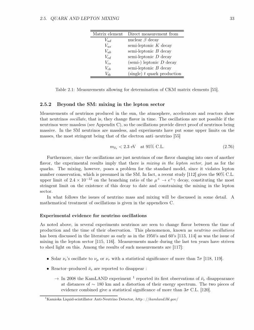
The different matrix elements are determined from the processes given in Table 2.1.The current values found in literature are [55]
VCKM ≃
|Vud| ≃ 0.97425 ± 0.00022 |Vus| ≃ 0.2252 ± 0.0009 |Vub| ≃ (3.89± 0.44) × 10−3
|Vcd| ≃ 0.230 ± 0.011 |Vcs| ≃ 1.023 ± 0.036 |Vcb| ≃ (40.6 ± 1.3) × 10−3
|Vtd| ≃ (8.4 ± 0.6)× 10−3 |Vts| ≃ (38.7 ± 2.1) × 10−3 |Vtb| ≃ 0.88 ± 0.07
.
(2.75)The most striking feature of Eq. (2.75) is that the diagonal elements Vud, Vcs, Vtb are clearlydominant.
2.5. QUARK AND LEPTON MIXING 33
Matrix element Direct measurement from
Vud nuclear β decayVus semi-leptonic K decayVub semi-leptonic B decayVcd semi-leptonic D decayVcs (semi-) leptonic D decayVcb semi-leptonic B decayVtb (single) t quark production
Table 2.1: Measurements allowing for determination of CKM matrix elements [55].
2.5.2 Beyond the SM: mixing in the lepton sector
Measurements of neutrinos produced in the sun, the atmosphere, accelerators and reactors showthat neutrinos oscillate, that is, they change flavor in time. The oscillations are not possible if theneutrinos were massless (see Appendix C), so the oscillations provide direct proof of neutrinos beingmassive. In the SM neutrinos are massless, and experiments have put some upper limits on themasses, the most stringent being that of the electron anti–neutrino [55]
mνe < 2.3 eV at 95% C.L. (2.76)
Furthermore, since the oscillations are just neutrinos of one flavor changing into ones of anotherflavor, the experimental results imply that there is mixing in the lepton sector, just as for thequarks. The mixing, however, poses a problem for the standard model, since it violates leptonnumber conservation, which is presumed in the SM. In fact, a recent study [112] gives the 90% C.L.upper limit of 2.4 × 10⁻¹² on the branching ratio of the µ+ → e+γ decay, constituting the moststringent limit on the existence of this decay to date and constraining the mixing in the leptonsector.
In what follows the issues of neutrino mass and mixing will be discussed in some detail. Amathematical treatment of oscillations is given in the appendices C.
Experimental evidence for neutrino oscillations
As noted above, in several experiments neutrinos are seen to change flavor between the time ofproduction and the time of their observation. This phenomenon, known as neutrino oscillationshas been discussed in the literature as early as in the 1950’s and 60’s [113, 114] as was the issue ofmixing in the lepton sector [115, 116]. Measurements made during the last ten years have strivento shed light on this. Among the results of such measurements are [117]:
• Solar νe’s oscillate to νµ or ντ with a statistical significance of more than 7σ [118, 119].
• Reactor–produced νe are reported to disappear :
→ In 2008 the KamLAND experiment 1 reported its first observations of νe disappearanceat distances of ∼ 180 km and a distortion of their energy spectrum. The two pieces ofevidence combined give a statistical significance of more than 3σ C.L. [120].
1Kamioka Liquid-scintillator Anti-Neutrino Detector, http : //kamland.lbl.gov/
34 CHAPTER 2. THE STANDARD MODEL
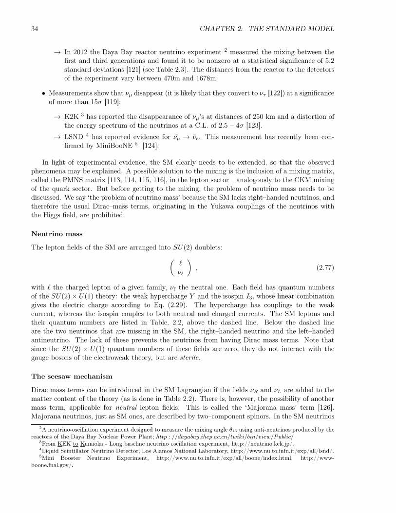
→ In 2012 the Daya Bay reactor neutrino experiment 2 measured the mixing between thefirst and third generations and found it to be nonzero at a statistical significance of 5.2standard deviations [121] (see Table 2.3). The distances from the reactor to the detectorsof the experiment vary between 470m and 1678m.
• Measurements show that νµ disappear (it is likely that they convert to ντ [122]) at a significanceof more than 15σ [119];
→ K2K 3 has reported the disappearance of νµ’s at distances of 250 km and a distortion ofthe energy spectrum of the neutrinos at a C.L. of 2.5 – 4σ [123].
→ LSND 4 has reported evidence for νµ → νe. This measurement has recently been con-firmed by MiniBooNE 5 [124].
In light of experimental evidence, the SM clearly needs to be extended, so that the observedphenomena may be explained. A possible solution to the mixing is the inclusion of a mixing matrix,called the PMNS matrix [113, 114, 115, 116], in the lepton sector – analogously to the CKM mixingof the quark sector. But before getting to the mixing, the problem of neutrino mass needs to bediscussed. We say ‘the problem of neutrino mass’ because the SM lacks right–handed neutrinos, andtherefore the usual Dirac–mass terms, originating in the Yukawa couplings of the neutrinos withthe Higgs field, are prohibited.
Neutrino mass
The lepton fields of the SM are arranged into SU(2) doublets:
(ℓνℓ
), (2.77)
with ℓ the charged lepton of a given family, νℓ the neutral one. Each field has quantum numbersof the SU(2)× U(1) theory: the weak hypercharge Y and the isospin I3, whose linear combinationgives the electric charge according to Eq. (2.29). The hypercharge has couplings to the weakcurrent, whereas the isospin couples to both neutral and charged currents. The SM leptons andtheir quantum numbers are listed in Table. 2.2, above the dashed line. Below the dashed lineare the two neutrinos that are missing in the SM, the right–handed neutrino and the left–handedantineutrino. The lack of these prevents the neutrinos from having Dirac mass terms. Note thatsince the SU(2) × U(1) quantum numbers of these fields are zero, they do not interact with thegauge bosons of the electroweak theory, but are sterile.
The seesaw mechanism
Dirac mass terms can be introduced in the SM Lagrangian if the fields νR and νL are added to thematter content of the theory (as is done in Table 2.2). There is, however, the possibility of anothermass term, applicable for neutral lepton fields. This is called the ‘Majorana mass’ term [126].Majorana neutrinos, just as SM ones, are described by two–component spinors. In the SM neutrinos
2A neutrino-oscillation experiment designed to measure the mixing angle θ13 using anti-neutrinos produced by thereactors of the Daya Bay Nuclear Power Plant; http : //dayabay.ihep.ac.cn/twiki/bin/view/Public/
3From KEK to Kamioka - Long baseline neutrino oscillation experiment, http://neutrino.kek.jp/.4Liquid Scintillator Neutrino Detector, Los Alamos National Laboratory, http://www.nu.to.infn.it/exp/all/lsnd/.5Mini Booster Neutrino Experiment, http://www.nu.to.infn.it/exp/all/boone/index.html, http://www-
boone.fnal.gov/.
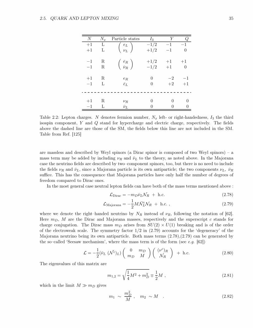
2.5. QUARK AND LEPTON MIXING 35
N Nx Particle states I3 Y Q
+1+1
LL
(eLνL
)−1/2+1/2
−1−1
−10
−1−1
RR
(eRνR
)+1/2−1/2
+1+1
+10
+1 R eR 0 −2 −1−1 L eL 0 +2 +1
+1 R νR 0 0 0−1 L νL 0 0 0
Table 2.2: Lepton charges. N denotes fermion number, Nx left- or right-handedness, I3 the thirdisospin component, Y and Q stand for hypercharge and electric charge, respectively. The fieldsabove the dashed line are those of the SM, the fields below this line are not included in the SM.Table from Ref. [125]
are massless and described by Weyl spinors (a Dirac spinor is composed of two Weyl spinors) – amass term may be added by including νR and νL to the theory, as noted above. In the Majoranacase the neutrino fields are described by two–component spinors, too, but there is no need to includethe fields νR and νL, since a Majorana particle is its own antiparticle; the two components νL, νRsuffice. This has the consequence that Majorana particles have only half the number of degrees offreedom compared to Dirac ones.
In the most general case neutral lepton fields can have both of the mass terms mentioned above :
LDirac = −mDνLNR + h.c. (2.78)
LMajorana = −1
2MN c
LNR + h.c. , (2.79)
where we denote the right–handed neutrino by NR instead of νR, following the notation of [62].Here mD, M are the Dirac and Majorana masses, respectively and the superscript c stands forcharge conjugation. The Dirac mass mD arises from SU(2) × U(1) breaking and is of the orderof the electroweak scale. The symmetry factor 1/2 in (2.79) accounts for the ‘degeneracy’ of theMajorana neutrino being its own antiparticle. Both mass terms (2.78),(2.79) can be generated bythe so–called ‘Seesaw mechanism’, where the mass term is of the form (see e.g. [62])
L = −1
2(νL ¯(N c)L)
(0 mD
mD M
)((νc)RNR
)+ h.c. (2.80)
The eigenvalues of this matrix are
m1,2 =
√1
4M2 +m2
D ∓ 1
2M , (2.81)
which in the limit M ≫ mD gives
m1 ∼ m2D
M, m2 ∼M . (2.82)
36 CHAPTER 2. THE STANDARD MODEL
The mixing angle θ depends on the mass eigenvalues [127]
tan θ =m1
mD=mD
m2=
√m1
m2(2.83)
and in the present limit it reads
tan θ ∼ mD
M. (2.84)
When mD is fixed and M is increased, the mixing angle tends to zero and the two different neutrinostates decouple. The Dirac mass is usually set proportional to the SM mass scale, whereas M isassociated with the scale of BSM physics. We recall that the LEP bounds presented previouslyimply that mν′ & mz/2 while the argument of naturalness restrics the Yukawa coupling of theneutrino to be O(1). This restricts the Dirac component of the fourth generation neutrino mass tomD ≃ O(100 − 500) GeV, which in turn implies that the mixing angle is approximately confinedinto the range [128]:
0.1 . tan θ . 1 . (2.85)
For more than one generation, the above considerations are generalized in a straightforwardmanner (see e.g. [62]). In the general n generation scenario, the mass matrix M is of size n×n andcomplex. An arbitrary M ∈ GL(N,C) is not necessarily positive definite but the operator MM † is.Hence there exists a matrix U ∈ U(N) such that [108]
MM † = Um2DU
† , (2.86)
with m2D = diag(m2
1, ...,m2N ), where m2
i are the eigenvalues of MM †. One can just as well useanother matrix V ∈ U(N) to perform the diagonalization
mD = U †MV . (2.87)
A similar unitary matrix appears in the mass term for the charged leptons [127], we denote thisby Uℓ. The product of the charged and neutral lepton matrices then becomes the analogue of theCKM matrix for the leptons, called the PMNS matrix [113, 114, 115, 116] :
UPMNS ≡ U †ℓU . (2.88)
The PMNS matrix
In order to investigate the leptonic mixing matrix, let us define weak and mass eigenfields νW andνM by
νW ≡
νeνµντ
and νM ≡
ν1ν2ν3
. (2.89)
The states that are physically observed are the ones taking part in interactions, that is, the statesνW . The two different bases in (2.89) are related by
νW = UνM . (2.90)
with U ∈ U(3) for three generations (see also Section 2.5.1 and Appendix C).
The Majorana case differs from the Dirac one in that the Majorana condition ν = νc does notallow a certain number of phases to be absorbed into neutrino phases. Only N phases, equal to the

2.5. QUARK AND LEPTON MIXING 37
number of charged leptons which are Dirac particles, can be absorbed into charged lepton phases,giving 1
2N(N − 1) unabsorbed phases. [127]There are several ways to parametrize the 3× 3 unitary matrix for three generations, depending
on whether the particles are Dirac or Majorana. One of these, perhaps the best known, is theCabibbo – Kobayashi – Maskawa (CKM) representation [23, 106]
UPMNS =
c12c13 s12c13 s13e−iδ
−s12c23 − c12s23s13eiδ c12c23 − s12s23s13e
iδ s23c13s12s23 − c12s23s13e
iδ −c12s23 − s12c23s13eiδ c23c13
×
1
eiα212
eiα312
(2.91)where cij ≡ cos θij, sij ≡ sin θij , the angles θij ∈ [0, π/2], the Dirac CP violating phase δ ∈ [0, π/2]and α21, α31 are the two Majorana CP violating phases [55]. The current values for the parameterssin θij are shown in Table 2.3. The value of the parameter δ is yet unknown.
Parameter Best fit ±1σ
sin2 θ12 0.312+0.017−0.015
sin2 θ230.51 ± 0.060.52 ± 0.06
sin2 θ13 0.092 ± 0.016(stat) ± 0.005(syst)
Table 2.3: Values of the neutrino mixing angles, with the statistical (stat) and systematical (syst)errors given separately for sin2 θ13. For sin2 θ23 the upper (lower) row corresponds to normal (in-verted) neutrino mass hierarchy. sin2 θ12 and sin2 θ23 values from Ref. [129], sin2 θ13 from Ref.[121].

38 CHAPTER 2. THE STANDARD MODEL

Part II
The minimal four–generation model
39

Chapter 3
Phenomenology of the fourth family
In this part we consider adding a sequential fourth generation of elementary particles to the standardmodel, sequential meaning that the fourth family has the same structure as the first three families.This means adding one quark and one lepton doublet to the SM :
quark doublet
(t′
b′
), lepton doublet
(ℓ′
ν ′ℓ
), (3.1)
such that the particles of (3.1) have the same quantum numbers as their counterparts in the firstthree families (the t′ quark is the fourth family ‘equivalent’ to the u, c, t quarks of the first, secondand third families, respectively, and so on). In the Introduction appealing features of this extensionwere considered; in this chapter we will focus on the phenomenological implications of and theexperimental constraints on a fourth family.
3.1 Mixing of the fourth family with the first three ones
As already discussed (see Section 2.5.1), the phenomenon of mixing in the quark sector is wellestablished in the SM. Apparently also the neutrinos ‘mix’ among themselves, as observed in theneutrino oscillations presented above (Section 2.5.2). It may seem natural that since the first threefamilies mix among themselves, that a sequential fourth generation would do so too. The mixingof the fourth family is constrained by both theoretical and experimental considerations, as we shallsee, but it is not ruled out by the already measured CKM matrix elements. The task of measuringwith better precision these parameters and determining the number of fermion families is one of thegoals of the LHC [63, 130]) and further at the ILC [131].
In this section we will often use the notation ‘CKM3’ and ‘CKM4’ to denote the 3× 3 and 4× 4mixing matrices of the three-generation and four-generation models, respectively.
3.1.1 Sources for constraints
CKM Unitarity
The 3 × 3 CKM submatrix is well tested by a variety of processes, as discussed previously (seeSection 2.5.1 and especially Table 2.1). The unitarity of the CKM matrix constrains the elementsof each row and column :
4∑
j=1
|V 2ij | = 1 for fixed i ,
4∑
i=1
|V 2ij | = 1 for fixed j . (3.2)
41
42 CHAPTER 3. PHENOMENOLOGY OF THE FOURTH FAMILY
When the currently measured values of the 3 × 3 matrix are taken into account, the unitarityconstraint (3.2) allows to deduce some of the mixing parameters [132]:
1st row : |Vub′ |2 = 1− |Vud|2 − |Vus|2 − |Vub|2 ≃ 0.0008 ± 0.0011 (3.3)
2nd row : |Vcb′ |2 = 1− |Vcd|2 − |Vcs|2 − |Vcb|2 ≃ −0.003 ± 0.027 (3.4)
1st column : |Vt′d|2 = 1− |Vud|2 − |Vcd|2 − |Vtd|2 ≃ −0.001 ± 0.005 . (3.5)
Requiring Eqs. (3.3)–(3.5) to be valid at 1σ one finds
|Vub′ | . 0.04 , |Vcb′ | . 0.17 , |Vt′d| . 0.08 . (3.6)
All of these are larger than the smallest elements of the CKM matrix, namely |Vub| and |Vtd| (seeEq. (2.75)).
Oblique electroweak corrections
Global fits to electroweak precision data serve to constrain the mixing between third and fourthfamily quarks. The dominant constraint comes from nondecoupling oblique corrections, denoted bythe parameters S, T, U (see Appendix D).
Two of the electroweak (EW) precision observables have a quadratic dependence on the masses ofthe fourth generation fermions and therefore serve to constrain the SM4: the ρ parameter [133, 134,135] correction through the oblique parameter T [136, 137] and the Zbb vertex correction (Fig. 3.1)
Rb =Γ(Z → bb)
Γ(Z → hadrons). (3.7)
This quantity is highly relevant in the study of the fourth generation because, as shown in Fig. 3.1,the Z → bb partial decay width has corrections from fourth–generation quark loops, in addition tothe oblique corrections [86]. This dependence differs from what is expected at 1–loop order in theSM [45]
δρ, δRb |SM ∝ GFm2t , (3.8)
δρ, δRb |SM4 ∝ |Vt′b|2 · (m2t′ −m2
t ) , (3.9)
evaluated from the nondecoupling vertex correction from the t +W diagrams. The correction of(3.9) is the one arising from 3–4 CKM mixing.
These relations serve to constrain the free parameters of the fourth generation, since they bothhave been measured with good precision. Specifically, the value of the rho–parameter is known tobe very close to one [59]:
ρ = 1.0004+0.0003−0.0004 , (3.10)
as obtained from global fits to electroweak precision data.If the mass splitting of the fourth quark doublet is large (m2
b′ ≫ m2t′) then there are also large
corrections proportional to |Vt′b|2m2b′ . [45]
Flavor changing neutral currents
Also processes including flavor changing neutral currents (FCNCs) constrain new–physics models.This is so because FCNCs are absent at tree level in the SM, thanks to the unitarity of the CKMmatrix and the inclusion of just one Higgs doublet (the case of two Higgs doublets will be discussed
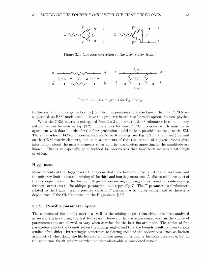
3.1. MIXING OF THE FOURTH FAMILY WITH THE FIRST THREE ONES 43
Z
t′
t′
W
b
b
Z
W
W
t′
b
b
Figure 3.1: One-loop correction to the Zbb –vertex from t′.
b
d
t, c, u W− t, c, u
d
b d
bt, c, u
t, c, u
W−d
b
Figure 3.2: Box diagrams for Bd mixing.
further on) and no new gauge bosons [138]. From experiments it is also known that the FCNCs aresuppressed, so BSM models should have this property in order to be valid options for new physics.
When the CKM matrix is enlargened from 3× 3 to 4× 4, the 3× 3 submatrix loses its unitarynature, as can be seen in Eq. (3.2). This allows for new FCNC processes, which must be inagreement with data in order for the four–generation model to be a possible extension to the SM.The amplitudes of FCNC processes, such as Bd or K mixing (see Fig. 3.2 for the former) dependon the CKM matrix elements, and so measurements of the cross section of a given process givesinformation about the matrix elements when all other parameters appearing in the amplitude areknown. This is an especially good method for observables that have been measured with highprecision.
Higgs mass
Measurements of the Higgs mass – the regions that have been excluded by LEP and Tevatron, andthe unitarity limit – constrain mixing of the third and fourth generations. As discussed above, part ofthe fits’ dependence on the third–fourth generation mixing angle θ34 comes from the nondecouplingfermion corrections to the oblique parameters, and especially T . The T parameter is furthermorerelated to the Higgs mass: a positive value of T pushes mH to higher values, and so there is adependence of the CKM4 entries on the Higgs mass. [139]
3.1.2 Possible parameter space
The elements of the mixing matrix as well as the mixing angles themselves have been analyzedin several studies during the last few years. However, there is some controversy in the choice ofparameters that are allowed to vary when searches for the best fits are made. The choice of freeparameters affects the bounds set on the mixing angles, and thus the bounds resulting from variousstudies often differ. Interestingly, sometimes neglecting some of the observables (such as hadronasymmetry) when doing the fits leads to an improvement in its quality for some observable, but atthe same time the fit gets worse when another observable is considered instead.
44 CHAPTER 3. PHENOMENOLOGY OF THE FOURTH FAMILY
In this section we attempt to review some of the results, emphasizing the choice of data thatis fitted and which variables are left free or possibly left out completely. We note that in light ofrecent results concerning the Higgs boson (see Chapter 5) some of the results below are alreadydated, but will be presented for the sake of academic interest nevertheless.
Quite sizeable mixings seem to be allowed in a study [111] that takes its experimentalconstraints from
(i) tree–level CKM3 elements in such a way as to restrict the CKM4 elements using
|Vi| − 2∆Vi < |VCKM4,i| < |Vi|+ 2∆Vi , (3.11)
where the Vi are the experimental values as given by the PDG [55], the errors being ∆Vi,
(ii) the unitarity of the CKM matrix,
(iii) the following FCNC processes: K,D,Bd and Bs –mixing, the decay b → sγ (see Fig. 3.2 forthe Feynman diagrams for Bd–mixing).
The choice for free and fixed parameters is:
(iv) the CP violating phases δ13, δ14 and δ24 are left unconstrained,
(v) mt′ is varied from 300 to 650 GeV, such that the fourth generation quark masses are relatedthrough
mb′ = mt′ − 55 GeV . (3.12)
Furthermore, some simplifying assumptions are made concerning the QCD corrections below, andany correlations with the lepton mixing matrix are neglected.
This choice of input parameters and experimental constrains seems to favor small mixing of thefourth generation with the other ones, but larger mixings are not excluded – in fact, there seems tobe a region of parameter space where sizeable mixing is allowed. The mixing angles θ14, θ24 and θ34are shown in Table 3.1, for both conservative and aggressive bounds.
Parameter Conservative bound Aggressive bound
θ14 ≤ 0.0535 ≤ 0.0364θ24 ≤ 0.144 ≤ 0.104θ34 ≤ 0.737 ≤ 0.736
Table 3.1: Allowed mixing angles, resulting from the analysis of Ref. [111]. The conservative boundsassume χ2/d.o.f. < 2, while for the aggressive constraints χ2/d.o.f. < 0.5 is required (see Eq. (A.1)for the definition of χ2).
New FCNC processes and the following two kinds of experimental constraints are takeninto account in the analysis of Ref. [138]:
(i) the measured values of CKM3, using conservative bounds (conservative meaning in this casethat the bounds are related to the experimental values that take the largest uncertaintiesinto account, and that the orthonormality constraints on the rows and columns of the CKM3matrix are not taken into account),

3.1. MIXING OF THE FOURTH FAMILY WITH THE FIRST THREE ONES 45
(ii) current bounds for FCNC processes.
When left–right symmetry is assumed (meaning that DL and DR in (2.71) are equal), the largestallowed mixings of the fourth generation may be computed, giving a CKM4 matrix :
V =
0.974 −0.227 0.003 −2.0× 10⁻³
0.227 0.973 −0.040 2.1× 10⁻²
0.007 0.044 0.920 −0.39−3.7× 10⁻⁴ −3.6× 10⁻³ 0.39 0.92
. (3.13)
It is worth noting that the large value of Vtb largely violates the ordinary 3× 3 unitarity conditionof the known mixing matrix. As is seen from Eq. (2.75), this element has not yet been measuredwith very good precision and the error ∆Vtb in (2.75) is quite large so the present situation allowsfor 0.90 ≤ Vtb ≤ 0.94. This is in part due to the insufficient statistics on the production rate ofheavy quarks and also to the small branching ratios of FCNC processes. The branching ratios aresmall not just because the matrix elements are small but because semileptonic top quark decays areenhanced by the same matrix elements. The LHC should allow for more precise measurements ofthe characteristics of heavy quarks, since these are expected to be produced in large numbers. Itmay be possible to reach a sensitivity of 10−5 or 10−6 for FCNC processes at the LHC, in whichcase the proposed matrix (3.13) may be verified or discarded. [138]
The two above reviewed studies are controversial when the experimental constraintsare taken to be those of electroweak precision data (EWPD) [45]. The analysis is based uponglobal fits to the EWPD, instead of focusing on just one observable. The global fits to the dataneed furthermore to be reevaluated entirely – it is not sufficient to use the magnitude of shifts fromthe values of parameters in the SM fit. In this way the minimum of χ2 may be at values that aresignificantly different from the SM fit and furthermore effects arising from statistical fluctuations andsystematic uncertainties are smaller. [45] Global fits, when reevaluated using the same parameterset that the LEP electroweak working group [81], namely varying four SM parameters :
mt, ∆α5, αs and mH , (3.14)
such that mH may vary freely between 10 GeV and 1 TeV. In (3.14) ∆α5 is the five flavor hadroniccontribution to the renormalization of the electromagnetic coupling at the Z–pole (note that mt >mZ so only five flavors contribute) and αs is the strong coupling ‘constant’. The parameter ∆α5 isthe dominant uncertainty in α(mZ). Differing from the LEP EWWG, the W width is neglected,since its precision is poor and this parameter has only a small effect on the results.
Setting the fourth generation quark masses to satisfy (3.12) and choosing m′ν = 100 GeV,
m′ℓ = 145 GeV, the global fits give results as shown in Fig. 3.3 and Table 3.2. Table 3.2 shows that
the limit on |s34| behaves as m−1t′ formt′ ≫ mt. For these fits the Higgs boson mass is mH = 790±30
GeV and the correction from the fourth generation to the oblique parameter T : T4 is 0.47 ± 0.01at 95% confidence level. In all the cases studied in [45] |Vtb| ≃ |Vt′b′ | ≃ | cos θ34| ≥ 0.94 and formt′ ≥ 500 GeV | cos θ34| ≥ 0.99, meaning that mixing between the third and fourth generation mightwell be of the order of Cabibbo mixing of the first two families. However, mixing angles as large asthose reported in [111], [138] are excluded by this analysis.
The upper limits of the mixing angles are not reported to depend sensitively on the choice ofmt′ − mb′ , but no acceptable fits are found for larger mass differences mt′ − mb′ & 100 GeV: at|s34| = 0 the fits are poor (CL(χ2)<0.03), and quickly become worse as |s34| increases. On theother hand, for smaller mass splittings, e.g. at the limiting case of mt′ = mb′ the confidence limits
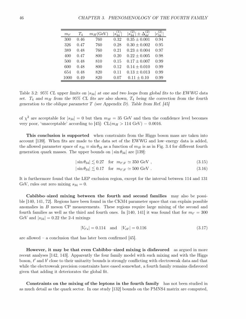
46 CHAPTER 3. PHENOMENOLOGY OF THE FOURTH FAMILY
mt′ T4 mH(GeV) |s(1)34 | |s(2)34 | ±∆(2)tb′ |c(2)34 |
300 0.46 760 0.32 0.35 ± 0.001 0.94326 0.47 760 0.28 0.30 ± 0.002 0.95389 0.48 760 0.21 0.23 ± 0.004 0.97400 0.47 800 0.20 0.22 ± 0.005 0.98500 0.48 810 0.15 0.17 ± 0.007 0.99600 0.48 800 0.12 0.14 ± 0.010 0.99654 0.48 820 0.11 0.13 ± 0.013 0.991000 0.49 820 0.07 0.11 ± 0.10 0.99
Table 3.2: 95% CL upper limits on |s34| at one and two loops from global fits to the EWWG dataset. T4 and mH from the 95% CL fits are also shown, T4 being the correction from the fourthgeneration to the oblique parameter T (see Appendix D). Table from Ref. [45]
of χ2 are acceptable for |s34| = 0 but then mH = 35 GeV and then the confidence level becomesvery poor, ‘unacceptable’ according to [45]: CL(mH > 114 GeV) = 0.0016.
This conclusion is supported when constraints from the Higgs boson mass are taken intoaccount [139]. When fits are made to the data set of the EWWG and low–energy data is added,the allowed parameter space of s34 ≡ sin θ34 as a function of mH is as in Fig. 3.4 for different fourthgeneration quark masses. The upper bounds on | sin θ34| are [139]:
| sin θ34| . 0.27 for mt′,b′ ≃ 350 GeV , (3.15)
| sin θ34| . 0.17 for mt′,b′ ≃ 500 GeV . (3.16)
It is furthermore found that the LEP exclusion region, except for the interval between 114 and 131GeV, rules out zero mixing s34 = 0.
Cabibbo–sized mixing between the fourth and second families may also be possi-ble [140, 141, 72]. Regions have been found in the CKM4 parameter space that can explain possibleanomalies in B meson CP measurements. These regions require large mixing of the second andfourth families as well as the third and fourth ones. In [140, 141] it was found that for mt′ = 300GeV and |s34| = 0.22 the 2-4 mixings
|Vt′s| = 0.114 and |Vcb′ | = 0.116 (3.17)
are allowed – a conclusion that has later been confirmed [45].
However, it may be that even Cabibbo–sized mixing is disfavored as argued in morerecent analyses [142, 143]. Apparently the four family model with such mixing and with the Higgsboson, t′ and b′ close to their unitarity bounds is strongly conflicting with electroweak data and thatwhile the electroweak precision constraints have eased somewhat, a fourth family remains disfavoredgiven that adding it deteriorates the global fit.
Constraints on the mixing of the leptons in the fourth family has not been studied inas much detail as the quark sector. In one study [132] bounds on the PMNS4 matrix are computed,
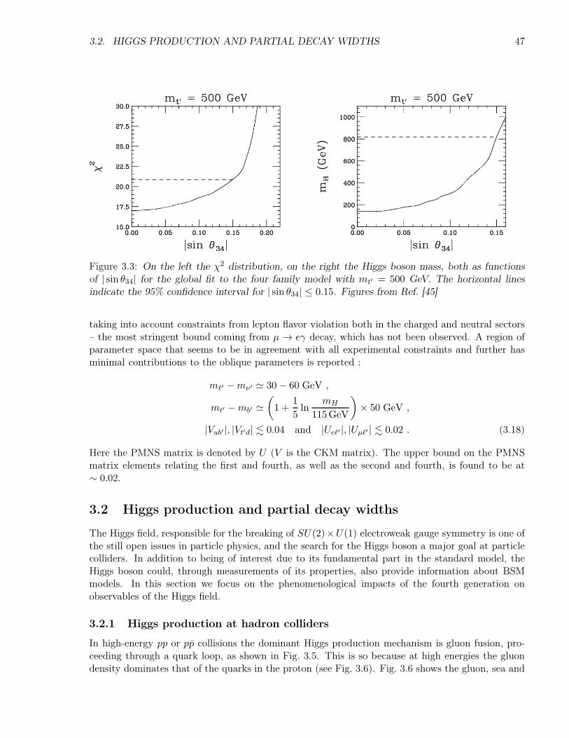
3.2. HIGGS PRODUCTION AND PARTIAL DECAY WIDTHS 47
Figure 3.3: On the left the χ2 distribution, on the right the Higgs boson mass, both as functionsof | sin θ34| for the global fit to the four family model with mt′ = 500 GeV. The horizontal linesindicate the 95% confidence interval for | sin θ34| ≤ 0.15. Figures from Ref. [45]
taking into account constraints from lepton flavor violation both in the charged and neutral sectors– the most stringent bound coming from µ → eγ decay, which has not been observed. A region ofparameter space that seems to be in agreement with all experimental constraints and further hasminimal contributions to the oblique parameters is reported :
mℓ′ −mν′ ≃ 30− 60 GeV ,
mt′ −mb′ ≃(1 +
1
5ln
mH
115GeV
)× 50 GeV ,
|Vub′ |, |Vt′d| . 0.04 and |Ueℓ′ |, |Uµℓ′ | . 0.02 . (3.18)
Here the PMNS matrix is denoted by U (V is the CKM matrix). The upper bound on the PMNSmatrix elements relating the first and fourth, as well as the second and fourth, is found to be at∼ 0.02.
3.2 Higgs production and partial decay widths
The Higgs field, responsible for the breaking of SU(2)×U(1) electroweak gauge symmetry is one ofthe still open issues in particle physics, and the search for the Higgs boson a major goal at particlecolliders. In addition to being of interest due to its fundamental part in the standard model, theHiggs boson could, through measurements of its properties, also provide information about BSMmodels. In this section we focus on the phenomenological impacts of the fourth generation onobservables of the Higgs field.
3.2.1 Higgs production at hadron colliders
In high-energy pp or pp collisions the dominant Higgs production mechanism is gluon fusion, pro-ceeding through a quark loop, as shown in Fig. 3.5. This is so because at high energies the gluondensity dominates that of the quarks in the proton (see Fig. 3.6). Fig. 3.6 shows the gluon, sea and
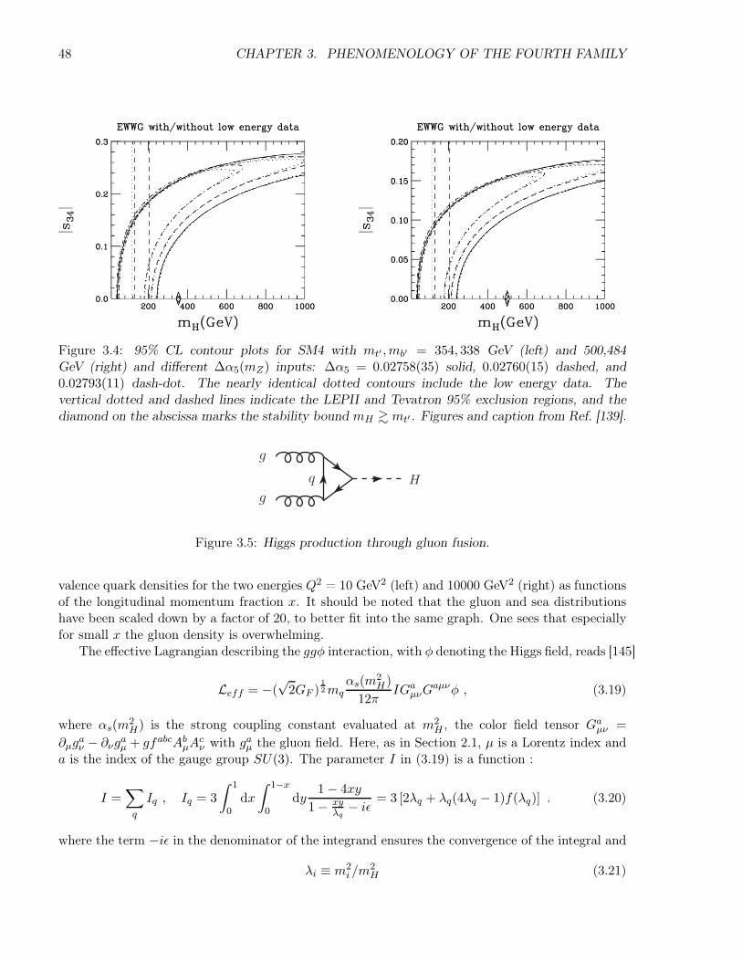
48 CHAPTER 3. PHENOMENOLOGY OF THE FOURTH FAMILY
Figure 3.4: 95% CL contour plots for SM4 with mt′ ,mb′ = 354, 338 GeV (left) and 500,484GeV (right) and different ∆α5(mZ) inputs: ∆α5 = 0.02758(35) solid, 0.02760(15) dashed, and0.02793(11) dash-dot. The nearly identical dotted contours include the low energy data. Thevertical dotted and dashed lines indicate the LEPII and Tevatron 95% exclusion regions, and thediamond on the abscissa marks the stability bound mH & mt′ . Figures and caption from Ref. [139].
g
g
Hq
Figure 3.5: Higgs production through gluon fusion.
valence quark densities for the two energies Q2 = 10 GeV2 (left) and 10000 GeV2 (right) as functionsof the longitudinal momentum fraction x. It should be noted that the gluon and sea distributionshave been scaled down by a factor of 20, to better fit into the same graph. One sees that especiallyfor small x the gluon density is overwhelming.
The effective Lagrangian describing the ggφ interaction, with φ denoting the Higgs field, reads [145]
Leff = −(√2GF )
1
2mqαs(m
2H)
12πIGa
µνGaµνφ , (3.19)
where αs(m2H) is the strong coupling constant evaluated at m2
H , the color field tensor Gaµν =
∂µgaν − ∂νg
aµ + gfabcAb
µAcν with gaµ the gluon field. Here, as in Section 2.1, µ is a Lorentz index and
a is the index of the gauge group SU(3). The parameter I in (3.19) is a function :
I =∑
q
Iq , Iq = 3
∫ 1
0dx
∫ 1−x
0dy
1− 4xy
1− xyλq
− iǫ= 3 [2λq + λq(4λq − 1)f(λq)] . (3.20)
where the term −iǫ in the denominator of the integrand ensures the convergence of the integral and
λi ≡ m2i /m
2H (3.21)
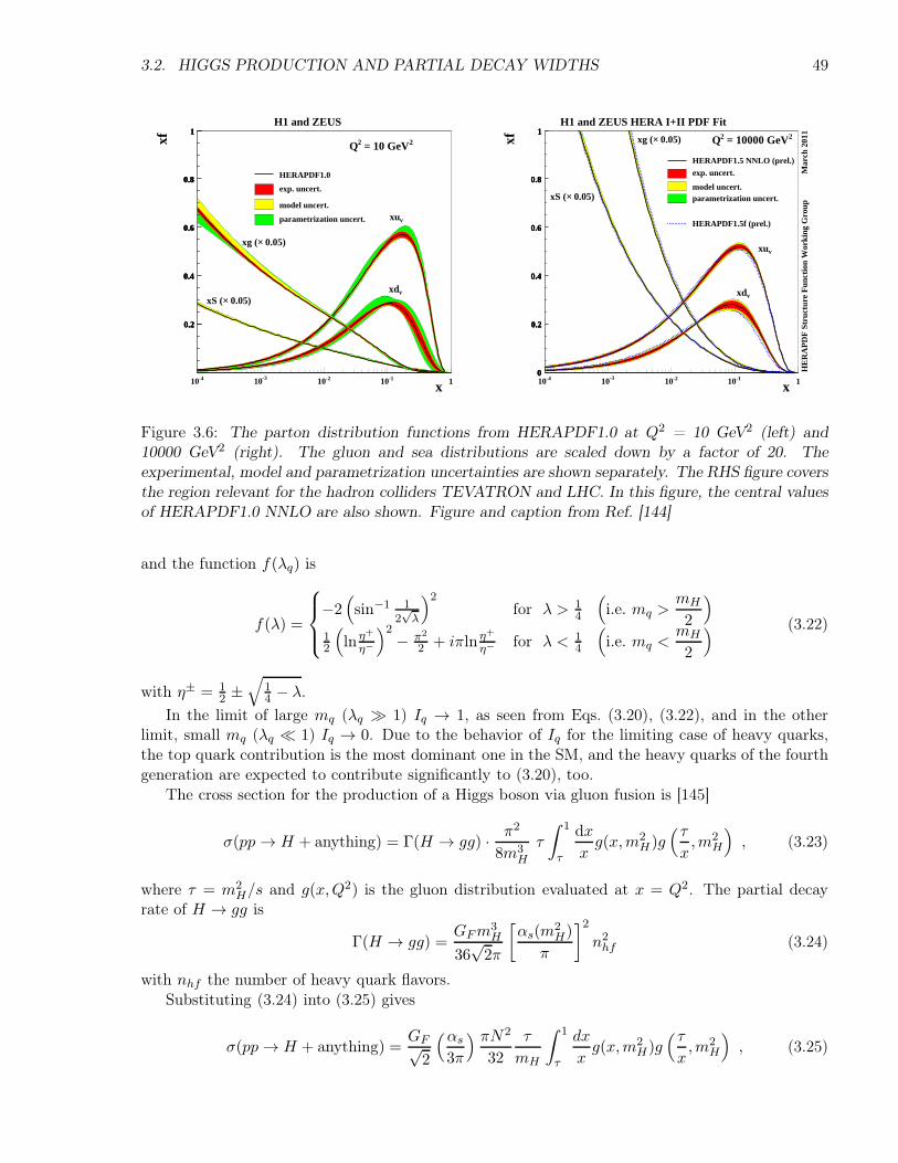
3.2. HIGGS PRODUCTION AND PARTIAL DECAY WIDTHS 49
0.2
0.4
0.6
0.8
1
-410 -310 -210 -110 1
0.2
0.4
0.6
0.8
1
HERAPDF1.0
exp. uncert.
model uncert.
parametrization uncert.
x
xf 2 = 10 GeV2Q
vxu
vxd 0.05)×xS (
0.05)×xg (
H1 and ZEUS
0.2
0.4
0.6
0.8
1
0
0.2
0.4
0.6
0.8
1
-410 -310 -210 -110 10
0.2
0.4
0.6
0.8
1
HERAPDF1.5 NNLO (prel.)
exp. uncert.
model uncert. parametrization uncert.
HERAPDF1.5f (prel.)
x
xf 2 = 10000 GeV2Q
vxu
vxd
0.05)×xS (
0.05)×xg (
HE
RA
PD
F S
truc
ture
Fun
ctio
n W
orki
ng G
roup
Mar
ch 2
011
H1 and ZEUS HERA I+II PDF Fit
0
0.2
0.4
0.6
0.8
1
Figure 3.6: The parton distribution functions from HERAPDF1.0 at Q2 = 10 GeV2 (left) and10000 GeV2 (right). The gluon and sea distributions are scaled down by a factor of 20. Theexperimental, model and parametrization uncertainties are shown separately. The RHS figure coversthe region relevant for the hadron colliders TEVATRON and LHC. In this figure, the central valuesof HERAPDF1.0 NNLO are also shown. Figure and caption from Ref. [144]
and the function f(λq) is
f(λ) =
−2(sin−1 1
2√λ
)2for λ > 1
4
(i.e. mq >
mH
2
)
12
(ln η+
η−
)2− π2
2 + iπln η+
η− for λ < 14
(i.e. mq <
mH
2
) (3.22)
with η± = 12 ±
√14 − λ.
In the limit of large mq (λq ≫ 1) Iq → 1, as seen from Eqs. (3.20), (3.22), and in the otherlimit, small mq (λq ≪ 1) Iq → 0. Due to the behavior of Iq for the limiting case of heavy quarks,the top quark contribution is the most dominant one in the SM, and the heavy quarks of the fourthgeneration are expected to contribute significantly to (3.20), too.
The cross section for the production of a Higgs boson via gluon fusion is [145]
σ(pp → H + anything) = Γ(H → gg) · π2
8m3H
τ
∫ 1
τ
dx
xg(x,m2
H )g(τx,m2
H
), (3.23)
where τ = m2H/s and g(x,Q2) is the gluon distribution evaluated at x = Q2. The partial decay
rate of H → gg is
Γ(H → gg) =GFm
3H
36√2π
[αs(m
2H)
π
]2n2hf (3.24)
with nhf the number of heavy quark flavors.
Substituting (3.24) into (3.25) gives
σ(pp→ H + anything) =GF√2
(αs
3π
) πN2
32
τ
mH
∫ 1
τ
dx
xg(x,m2
H)g(τx,m2
H
), (3.25)
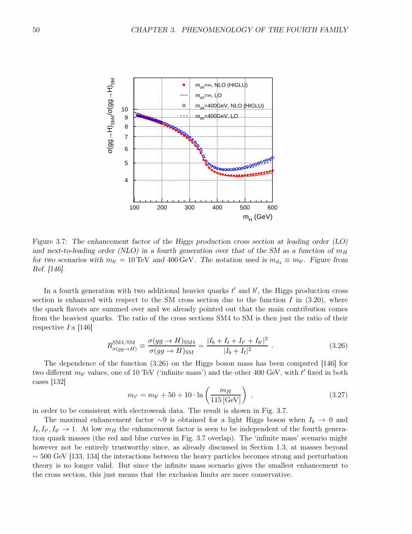
50 CHAPTER 3. PHENOMENOLOGY OF THE FOURTH FAMILY
4
5
6
7
8
910
100 200 300 400 500 600
mH (GeV)
σ(gg
→H
) SM
4/σ(
gg→
H) S
M
md4=∞, NLO (HIGLU)
md4=∞, LO
md4=400GeV, NLO (HIGLU)
md4=400GeV, LO
Figure 3.7: The enhancement factor of the Higgs production cross section at leading order (LO)and next-to-leading order (NLO) in a fourth generation over that of the SM as a function of mH
for two scenarios with mb′ = 10TeV and 400GeV. The notation used is md4 ≡ mb′ . Figure fromRef. [146].
In a fourth generation with two additional heavier quarks t′ and b′, the Higgs production crosssection is enhanced with respect to the SM cross section due to the function I in (3.20), wherethe quark flavors are summed over and we already pointed out that the main contribution comesfrom the heaviest quarks. The ratio of the cross sections SM4 to SM is then just the ratio of theirrespective I:s [146]
RSM4/SMσ(gg→H) ≡
σ(gg → H)SM4
σ(gg → H)SM=
|Ib + It + It′ + Ib′ |2|Ib + It|2
. (3.26)
The dependence of the function (3.26) on the Higgs boson mass has been computed [146] fortwo different mb′ values, one of 10 TeV (‘infinite mass’) and the other 400 GeV, with t′ fixed in bothcases [132]
mt′ = mb′ + 50 + 10 · ln(
mH
115 [GeV]
), (3.27)
in order to be consistent with electroweak data. The result is shown in Fig. 3.7.The maximal enhancement factor ∼9 is obtained for a light Higgs boson when Ib → 0 and
It, It′ , Ib′ → 1. At low mH the enhancement factor is seen to be independent of the fourth genera-tion quark masses (the red and blue curves in Fig. 3.7 overlap). The ‘infinite mass’ scenario mighthowever not be entirely trustworthy since, as already discussed in Section 1.3, at masses beyond∼ 500 GeV [133, 134] the interactions between the heavy particles becomes strong and perturbationtheory is no longer valid. But since the infinite mass scenario gives the smallest enhancement tothe cross section, this just means that the exclusion limits are more conservative.

3.2. HIGGS PRODUCTION AND PARTIAL DECAY WIDTHS 51
(GeV)4
qm200 400 600 800 1000 1200 1400 1600
(pb
)σ
1
10
210
(GeV)hm
120
300
500
1000
Figure 3.8: The Higgs boson production cross section for different Higgs masses as a function ofthe fourth generation quark mass mq′ (the fourth generation quarks are taken to be degenerate).Figure from Ref. [148].
When the fourth generation quarks are very heavy with respect to the Higgs, mq′ ≫ mH ,the Higgs coupling cancels the mass dependence of each of the three propagators of the quarkloop. Hence the ggφ coupling is asymptotically independent of the masses of the fourth generationquarks. [147] This can be seen in Fig. 3.8 for the case of a degenerate fourth generation [148]. It isinteresting to note that for mH ≤ 300 GeV the cross section seems to be independent of mq′ (thethree upmost curves in Fig. 3.8 are nearly horizontal).
3.2.2 Branching fractions
In particle detectors the Higgs will be indirectly seen from its decay products. When the numberof events in the various channels is known, the branching fractions can be computed, giving in turnvaluable information about the couplings. The presence of a fourth generation may affect the Higgsdecays in such a way that the branching fractions differ from those predicted by the standard model.If so, this will be a measurable effect and hence the discovery of the Higgs and the measurementof its branching ratios will give information about the fourth generation and vice versa: the fourthgeneration also affects, through loops, Higgs pair production and the Higgs self coupling.
Higgs decay to two photons
The H → γγ is similar to H → gg considered above (Eq. (3.24)), except that charged leptons,the W boson and the charged Higgs bosons also contribute to the loop. The effective Lagrangian,obtained from the low energy theorem, is then [145]
Leff = − α
8π(√2GF )
1
2 IFµνFµνH (3.28)
and the H → γγ decay rate is
Γ(H → γγ) =GFm
3H
8√2π
(απ
)2|I|2 . (3.29)
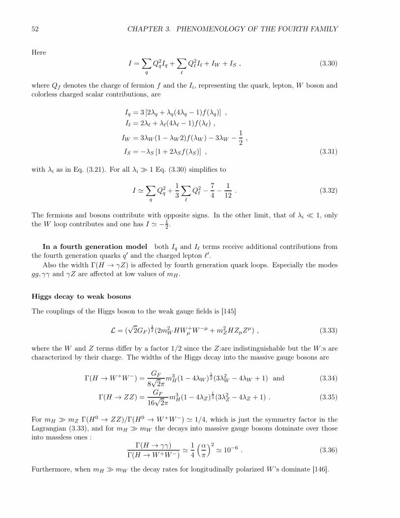
52 CHAPTER 3. PHENOMENOLOGY OF THE FOURTH FAMILY
Here
I =∑
q
Q2qIq +
∑
ℓ
Q2ℓIℓ + IW + IS , (3.30)
where Qf denotes the charge of fermion f and the Ii, representing the quark, lepton, W boson andcolorless charged scalar contributions, are
Iq = 3 [2λq + λq(4λq − 1)f(λq)] ,
Iℓ = 2λℓ + λℓ(4λℓ − 1)f(λℓ) ,
IW = 3λW (1− λW2)f(λW )− 3λW − 1
2,
IS = −λS [1 + 2λSf(λS)] , (3.31)
with λi as in Eq. (3.21). For all λi ≫ 1 Eq. (3.30) simplifies to
I ≃∑
q
Q2q +
1
3
∑
ℓ
Q2ℓ −
7
4− 1
12. (3.32)
The fermions and bosons contribute with opposite signs. In the other limit, that of λi ≪ 1, onlythe W loop contributes and one has I ≃ −1
2 .
In a fourth generation model both Iq and Iℓ terms receive additional contributions fromthe fourth generation quarks q′ and the charged lepton ℓ′.
Also the width Γ(H → γZ) is affected by fourth generation quark loops. Especially the modesgg, γγ and γZ are affected at low values of mH .
Higgs decay to weak bosons
The couplings of the Higgs boson to the weak gauge fields is [145]
L = (√2GF )
1
2 (2m2WHW
+µ W
−µ +m2ZHZµZ
µ) , (3.33)
where the W and Z terms differ by a factor 1/2 since the Z:are indistinguishable but the W :s arecharacterized by their charge. The widths of the Higgs decay into the massive gauge bosons are
Γ(H →W+W−) =GF
8√2πm3
H(1− 4λW )1
2 (3λ2W − 4λW + 1) and (3.34)
Γ(H → ZZ) =GF
16√2πm3
H(1− 4λZ)1
2 (3λ2Z − 4λZ + 1) . (3.35)
For mH ≫ mZ Γ(H0 → ZZ)/Γ(H0 → W+W−) ≃ 1/4, which is just the symmetry factor in theLagrangian (3.33), and for mH ≫ mW the decays into massive gauge bosons dominate over thoseinto massless ones :
Γ(H → γγ)
Γ(H →W+W−)≃ 1
4
(απ
)2≃ 10−6 . (3.36)
Furthermore, when mH ≫ mW the decay rates for longitudinally polarized W ’s dominate [146].
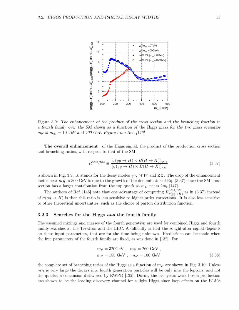
3.2. HIGGS PRODUCTION AND PARTIAL DECAY WIDTHS 53
0
2
4
6
8
10
12
100 200 300 400 500 600
mH (GeV)(σ(g
g→H
)xB
(H→
X))
SM
4/(σ
(gg→
H)x
B(H
→X
))S
M
γγ (md4=10TeV)
γγ (md4=400GeV)
WW, ZZ (md4=10TeV)
WW, ZZ (md4=400GeV)
Figure 3.9: The enhancement of the product of the cross section and the branching fraction ina fourth family over the SM shown as a function of the Higgs mass for the two mass scenariosmb′ ≡ md4 = 10 TeV and 400 GeV. Figure from Ref. [146]
The overall enhancement of the Higgs signal, the product of the production cross sectionand branching ratios, with respect to that of the SM
RSM4/SM ≡ [σ(gg → H)×B(H → X)]SM4
[σ(gg → H)×B(H → X)]SM(3.37)
is shown in Fig. 3.9. X stands for the decay modes γγ, WW and ZZ. The drop of the enhancementfactor near mH ≈ 300 GeV is due to the growth of the denominator of Eq. (3.37) since the SM crosssection has a larger contribution from the top quark as mH nears 2mt [147].
The authors of Ref. [146] note that one advantage of computing RSM4/SMσ(gg→H) as in (3.37) instead
of σ(gg → H) is that this ratio is less sensitive to higher order corrections. It is also less sensitiveto other theoretical uncertainties, such as the choice of parton distribution function.
3.2.3 Searches for the Higgs and the fourth family
The assumed mixings and masses of the fourth generation are used for combined Higgs and fourthfamily searches at the Tevatron and the LHC. A difficulty is that the sought-after signal dependson these input parameters, that are for the time being unknown. Predictions can be made whenthe free parameters of the fourth family are fixed, as was done in [132]. For
mt′ = 320GeV , mb′ = 260 GeV ,
mℓ′ = 155 GeV , mν′ = 100 GeV (3.38)
the complete set of branching ratios of the Higgs as a function of mH are shown in Fig. 3.10. UnlessmH is very large the decays into fourth generation particles will be only into the leptons, and notthe quarks, a conclusion disfavored by EWPD [132]. During the last years weak boson productionhas shown to be the leading discovery channel for a light Higgs since loop effects on the WWφ
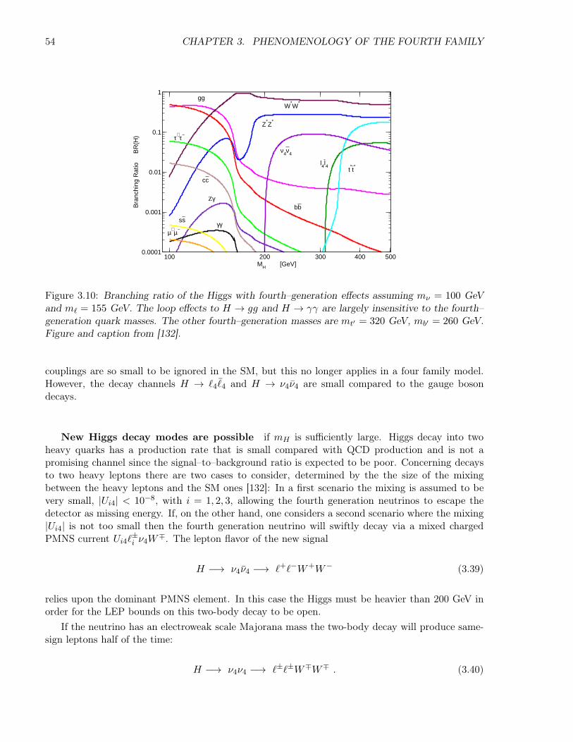
54 CHAPTER 3. PHENOMENOLOGY OF THE FOURTH FAMILY
200 300 400 500100MH [GeV]
0.0001
0.001
0.01
0.1
1
Bra
nchi
ng R
atio
B
R(H
)
γγ
Zγ
ss
µ+µ−
Z*Z
*
W*W
*
l4l4t*t*
gg
bb
τ+τ−
cc
ν4ν4
Figure 3.10: Branching ratio of the Higgs with fourth–generation effects assuming mν = 100 GeVand mℓ = 155 GeV. The loop effects to H → gg and H → γγ are largely insensitive to the fourth–generation quark masses. The other fourth–generation masses are mt′ = 320 GeV, mb′ = 260 GeV.Figure and caption from [132].
couplings are so small to be ignored in the SM, but this no longer applies in a four family model.However, the decay channels H → ℓ4ℓ4 and H → ν4ν4 are small compared to the gauge bosondecays.
New Higgs decay modes are possible if mH is sufficiently large. Higgs decay into twoheavy quarks has a production rate that is small compared with QCD production and is not apromising channel since the signal–to–background ratio is expected to be poor. Concerning decaysto two heavy leptons there are two cases to consider, determined by the the size of the mixingbetween the heavy leptons and the SM ones [132]: In a first scenario the mixing is assumed to bevery small, |Ui4| < 10−8, with i = 1, 2, 3, allowing the fourth generation neutrinos to escape thedetector as missing energy. If, on the other hand, one considers a second scenario where the mixing|Ui4| is not too small then the fourth generation neutrino will swiftly decay via a mixed chargedPMNS current Ui4ℓ
±i ν4W
∓. The lepton flavor of the new signal
H −→ ν4ν4 −→ ℓ+ℓ−W+W− (3.39)
relies upon the dominant PMNS element. In this case the Higgs must be heavier than 200 GeV inorder for the LEP bounds on this two-body decay to be open.
If the neutrino has an electroweak scale Majorana mass the two-body decay will produce same-sign leptons half of the time:
H −→ ν4ν4 −→ ℓ±ℓ±W∓W∓ . (3.40)
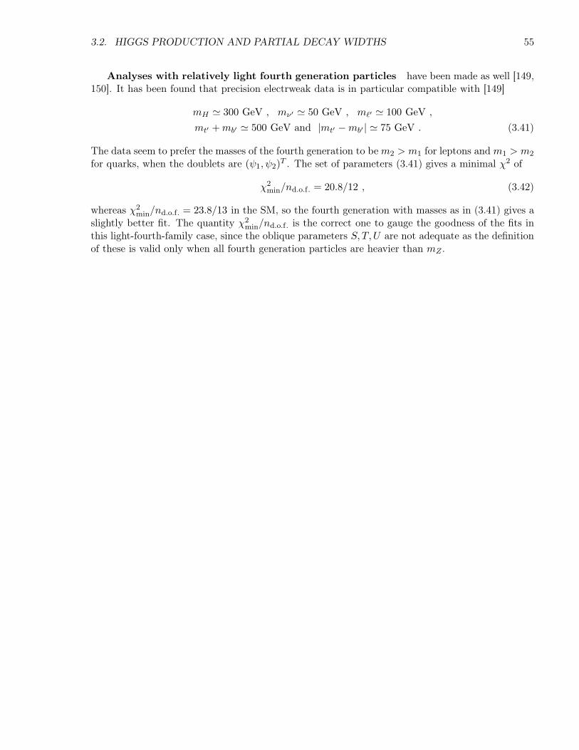
3.2. HIGGS PRODUCTION AND PARTIAL DECAY WIDTHS 55
Analyses with relatively light fourth generation particles have been made as well [149,150]. It has been found that precision electrweak data is in particular compatible with [149]
mH ≃ 300 GeV , mν′ ≃ 50 GeV , mℓ′ ≃ 100 GeV ,
mt′ +mb′ ≃ 500 GeV and |mt′ −mb′ | ≃ 75 GeV . (3.41)
The data seem to prefer the masses of the fourth generation to be m2 > m1 for leptons and m1 > m2
for quarks, when the doublets are (ψ1, ψ2)T . The set of parameters (3.41) gives a minimal χ2 of
χ2min/nd.o.f. = 20.8/12 , (3.42)
whereas χ2min/nd.o.f. = 23.8/13 in the SM, so the fourth generation with masses as in (3.41) gives a
slightly better fit. The quantity χ2min/nd.o.f. is the correct one to gauge the goodness of the fits in
this light-fourth-family case, since the oblique parameters S, T, U are not adequate as the definitionof these is valid only when all fourth generation particles are heavier than mZ .

56 CHAPTER 3. PHENOMENOLOGY OF THE FOURTH FAMILY
Chapter 4
Experimental searches
Running experiments test the standard model and physics beyond the SM. These searches – mainlydone at the LHC and Tevatron – include the fourth generation. At the LHC parton interactions ats ∼ 1 TeV will be produced in significant rates [151] so it is well suited for the search of new, heavyparticles. Specifically, such high–energy parton interactions may produce fourth generation particlesof masses close to the unitarity scale ∼ 500 GeV. In what follows we will review proposed searchstrategies and already existing bounds on the physics of a possible fourth generation. Feynmandiagrams of various production processes are shown in Appendix E.
4.1 Search strategies – SM4 quarks
In this section we will review the searches proposed for finding t′ and b′ quarks, both in single andpair production. We start by reviewing the event topologies [151] and then present studies thatwere made for identifying W bosons originating from heavy quark decays in pp collisions (at theLHC) [130] or in the process eq → t′ν (at the LHeC) [152]. It is of great interest to study both singleand pair production, since the two give different information: pair production allows for precise massmeasurements whereas single production gives information about the mixing of the fourth familywith the others [153]. Measuring both processes allows for a more comprehensive physical picture ofthe fourth generation. Also, the various production mechanisms give different information about thequarks: strong production depends only on the masses of the fourth generation quarks, whereas theelectroweak production and decay modes are mostly sensitive to the mass difference of the quarksand their CKM mixing [154].
4.1.1 General event topologies
For the fourth generation quark masses ∼ 400 − 600 GeV considered throughout this report thedominant decays are into a W boson and a light quark [151]. There are several possibilities for suchdecays:
(i) Q −→ qW
(ii) Q −→ qWW (4.1)
(iii) Q −→ qWWW
(4.2)
Here Q is a heavy quark (either t′ or b′) and q is one of the five lightest quarks (u, d, s, c, b). Thesedifferent channels occur for :
57
58 CHAPTER 4. EXPERIMENTAL SEARCHES
(i) This channel is especially seen for t′ −→ b, s, d + W or b′ −→ c, u + W . When the CKMmixing matrix is such that Vt′b ≪ Vcb′ and/or Vub′ then this is the dominant b′ decay channel.
(ii) This is the dominant b′ decay channel if the process begins by b′ −→ tW , followed by t −→ bW .There is a similar channel for t′, open when mt′ > mb′ +mW and the b′ decays through
b′ −→Wc or Wu such that t′ −→ WWc or WWu. (4.3)
(iii) This is the appropriate channel if t′ −→ Wb′ by process (i) and then b′ decays as in (ii):b′ −→Wt −→WWb.
Under certain conditions there may be important three–body decays. This is the case whenthe mixing between the third and fourth generations is small and the mass splitting between thet′ and b′ quarks is smaller than the W mass. Then the fourth generation quarks may also decaythrough [151]
(iv) Q −→ Q′W ∗ −→ qWW ∗ (4.4)
where W ∗ indicates a virtual W and Q is the heavier fourth generation quark, Q′ the lighter one.If mt′ > mb′ then the above chain gives t′ → b′W ∗ → tWW ∗ → bWWW ∗.
What happens to the W s and the light quarks?The light quarks form jets and the W has the following decays W+ (W−) −→ ℓ+νℓ (ℓ−νℓ) andW± −→ qq, called leptonic and hadronic channels, respectively. Hence a W+W− pair can decayin three distinct ways
leptonic : W+W− −→ ℓ+νℓ ℓ−νℓ
hadronic : W+W− −→ q1q1q2q2 (4.5)
semi− leptonic : W+W− −→ ℓ+νℓqq .
(4.6)
The quarks of the hadronic and semi–leptonic decays give rise to jets, which are a challenge froman experimental point of view. The leptons are easier to identify.
4.1.2 Pair production of fourth family quarks
A few years ago the signal of pair produced quarks decaying weakly was analyzed [130] – the signalbeing f fW+W−, with f typically a bottom or top quark. In this study the focus is on the case ofthe bottom quark, assuming that this (bbW+W−) would be the dominant decay mode of a fourthgeneration quark that has CKM mixings with the other generations.
The t′ quark is assumed to have a mass in the range 600–800 GeV, in which case its width wouldbe approximately 60 · |Vt′b|2 GeV, implying that it is possible that Γt′ < Γt if |Vt′b| is small. Theauthors note that both t′t′ (see Fig. E.1 (a) and (b)) and tt have the same final states and thatit is imperative to have an event selection that significantly reduces the tt background since thett cross section at the LHC is about 500 times larger than that of t′t′. To this aim the followingcharacteristics are demanded for a signal to pass the event selection :
− A lower bound Λtop5 = 2mt′ is put on the scalar pT sum of a number (e.g. five) of the hardestreconstructed objects in the detector,
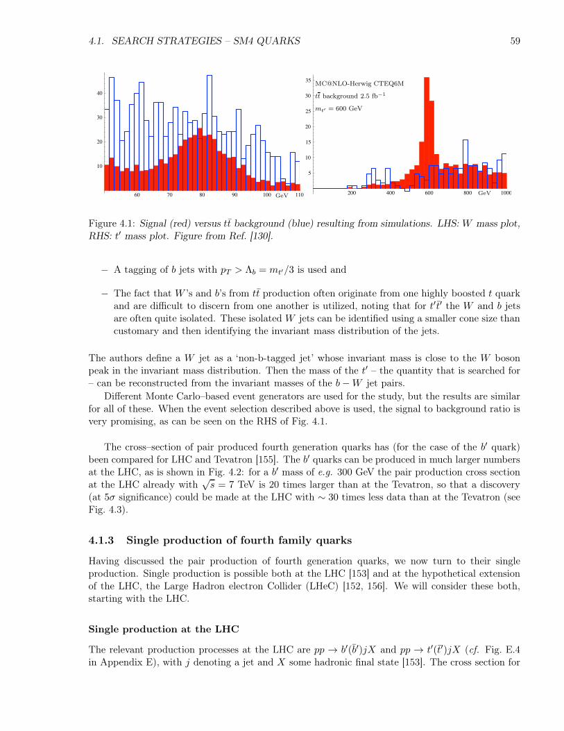
4.1. SEARCH STRATEGIES – SM4 QUARKS 59
Figure 4.1: Signal (red) versus tt background (blue) resulting from simulations. LHS: W mass plot,RHS: t′ mass plot. Figure from Ref. [130].
− A tagging of b jets with pT > Λb = mt′/3 is used and
− The fact that W ’s and b’s from tt production often originate from one highly boosted t quarkand are difficult to discern from one another is utilized, noting that for t′t′ the W and b jetsare often quite isolated. These isolated W jets can be identified using a smaller cone size thancustomary and then identifying the invariant mass distribution of the jets.
The authors define a W jet as a ‘non-b-tagged jet’ whose invariant mass is close to the W bosonpeak in the invariant mass distribution. Then the mass of the t′ – the quantity that is searched for– can be reconstructed from the invariant masses of the b−W jet pairs.
Different Monte Carlo–based event generators are used for the study, but the results are similarfor all of these. When the event selection described above is used, the signal to background ratio isvery promising, as can be seen on the RHS of Fig. 4.1.
The cross–section of pair produced fourth generation quarks has (for the case of the b′ quark)been compared for LHC and Tevatron [155]. The b′ quarks can be produced in much larger numbersat the LHC, as is shown in Fig. 4.2: for a b′ mass of e.g. 300 GeV the pair production cross sectionat the LHC already with
√s = 7 TeV is 20 times larger than at the Tevatron, so that a discovery
(at 5σ significance) could be made at the LHC with ∼ 30 times less data than at the Tevatron (seeFig. 4.3).
4.1.3 Single production of fourth family quarks
Having discussed the pair production of fourth generation quarks, we now turn to their singleproduction. Single production is possible both at the LHC [153] and at the hypothetical extensionof the LHC, the Large Hadron electron Collider (LHeC) [152, 156]. We will consider these both,starting with the LHC.
Single production at the LHC
The relevant production processes at the LHC are pp → b′(b′)jX and pp → t′(t′)jX (cf. Fig. E.4in Appendix E), with j denoting a jet and X some hadronic final state [153]. The cross section for
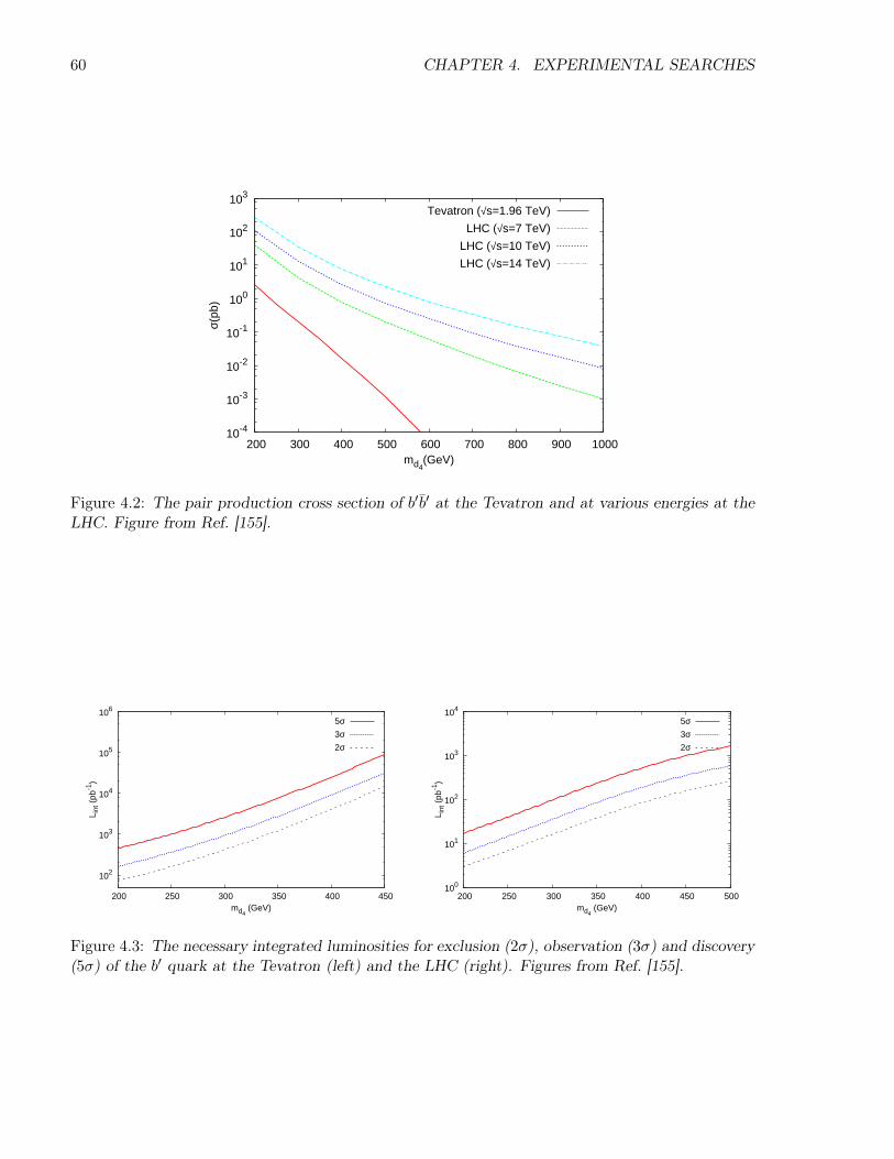
60 CHAPTER 4. EXPERIMENTAL SEARCHES
10-4
10-3
10-2
10-1
100
101
102
103
200 300 400 500 600 700 800 900 1000
σ(pb
)
md4(GeV)
Tevatron (√s=1.96 TeV)
LHC (√s=7 TeV)
LHC (√s=10 TeV)
LHC (√s=14 TeV)
Figure 4.2: The pair production cross section of b′b′ at the Tevatron and at various energies at theLHC. Figure from Ref. [155].
102
103
104
105
106
200 250 300 350 400 450
L int
(pb
-1)
md4 (GeV)
5σ3σ2σ
100
101
102
103
104
200 250 300 350 400 450 500
L int
(pb
-1)
md4 (GeV)
5σ3σ2σ
Figure 4.3: The necessary integrated luminosities for exclusion (2σ), observation (3σ) and discovery(5σ) of the b′ quark at the Tevatron (left) and the LHC (right). Figures from Ref. [155].
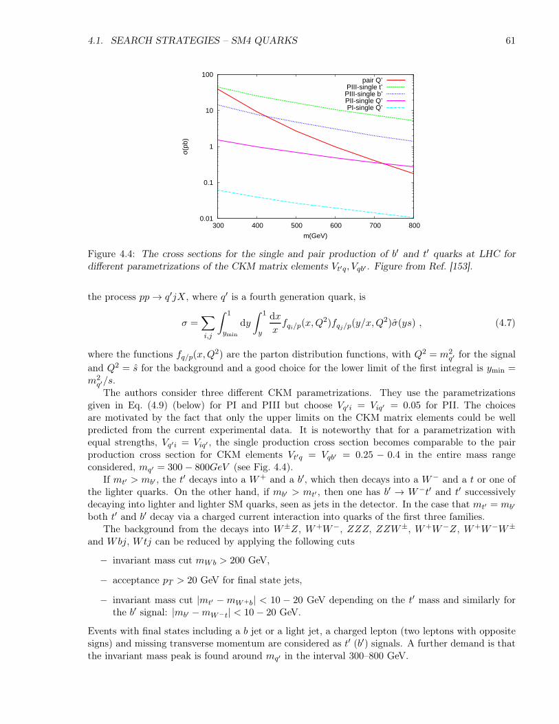
4.1. SEARCH STRATEGIES – SM4 QUARKS 61
0.01
0.1
1
10
100
300 400 500 600 700 800
σ(pb
)
m(GeV)
pair Q’PIII-single t’PIII-single b’PII-single Q’PI-single Q’
Figure 4.4: The cross sections for the single and pair production of b′ and t′ quarks at LHC fordifferent parametrizations of the CKM matrix elements Vt′q, Vqb′ . Figure from Ref. [153].
the process pp→ q′jX, where q′ is a fourth generation quark, is
σ =∑
i,j
∫ 1
ymin
dy
∫ 1
y
dx
xfqi/p(x,Q
2)fqj/p(y/x,Q2)σ(ys) , (4.7)
where the functions fq/p(x,Q2) are the parton distribution functions, with Q2 = m2
q′ for the signal
and Q2 = s for the background and a good choice for the lower limit of the first integral is ymin =m2
q′/s.The authors consider three different CKM parametrizations. They use the parametrizations
given in Eq. (4.9) (below) for PI and PIII but choose Vq′i = Viq′ = 0.05 for PII. The choicesare motivated by the fact that only the upper limits on the CKM matrix elements could be wellpredicted from the current experimental data. It is noteworthy that for a parametrization withequal strengths, Vq′i = Viq′ , the single production cross section becomes comparable to the pairproduction cross section for CKM elements Vt′q = Vqb′ = 0.25 − 0.4 in the entire mass rangeconsidered, mq′ = 300 − 800GeV (see Fig. 4.4).
If mt′ > mb′ , the t′ decays into a W+ and a b′, which then decays into a W− and a t or one ofthe lighter quarks. On the other hand, if mb′ > mt′ , then one has b′ → W−t′ and t′ successivelydecaying into lighter and lighter SM quarks, seen as jets in the detector. In the case that mt′ = mb′
both t′ and b′ decay via a charged current interaction into quarks of the first three families.The background from the decays into W±Z, W+W−, ZZZ, ZZW±, W+W−Z, W+W−W±
and Wbj, Wtj can be reduced by applying the following cuts
− invariant mass cut mWb > 200 GeV,
− acceptance pT > 20 GeV for final state jets,
− invariant mass cut |mt′ −mW+b| < 10 − 20 GeV depending on the t′ mass and similarly forthe b′ signal: |mb′ −mW−t| < 10− 20 GeV.
Events with final states including a b jet or a light jet, a charged lepton (two leptons with oppositesigns) and missing transverse momentum are considered as t′ (b′) signals. A further demand is thatthe invariant mass peak is found around mq′ in the interval 300–800 GeV.
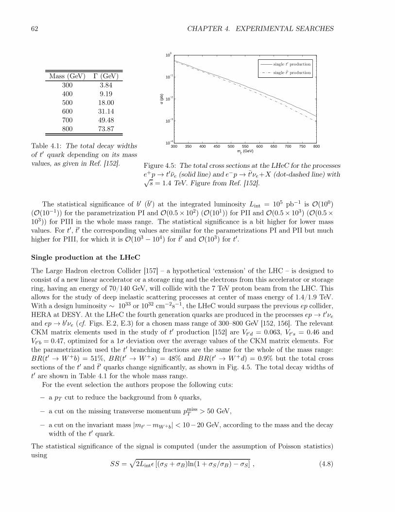
62 CHAPTER 4. EXPERIMENTAL SEARCHES
Mass (GeV) Γ (GeV)
300 3.84400 9.19500 18.00600 31.14700 49.48800 73.87
Table 4.1: The total decay widthsof t′ quark depending on its massvalues, as given in Ref. [152].
300 350 400 450 500 550 600 650 700 750 80010
−4
10−3
10−2
10−1
100
mt’ (GeV)
σ (p
b)
single t′ production
single t′ production
Figure 4.5: The total cross sections at the LHeC for the processese+p→ t′νe (solid line) and e−p→ t′νe+X (dot-dashed line) with√s = 1.4 TeV. Figure from Ref. [152].
The statistical significance of b′ (b′) at the integrated luminosity Lint = 105 pb−1 is O(100)(O(10−1)) for the parametrization PI and O(0.5× 10²) (O(101)) for PII and O(0.5× 10³) (O(0.5×10³)) for PIII in the whole mass range. The statistical significance is a bit higher for lower massvalues. For t′, t′ the corresponding values are similar for the parametrizations PI and PII but muchhigher for PIII, for which it is O(103 − 104) for t′ and O(103) for t′.
Single production at the LHeC
The Large Hadron electron Collider [157] – a hypothetical ‘extension’ of the LHC – is designed toconsist of a new linear accelerator or a storage ring and the electrons from this accelerator or storagering, having an energy of 70/140 GeV, will collide with the 7 TeV proton beam from the LHC. Thisallows for the study of deep inelastic scattering processes at center of mass energy of 1.4/1.9 TeV.With a design luminosity ∼ 1033 or 1032 cm−2s−1, the LHeC would surpass the previous ep collider,HERA at DESY. At the LHeC the fourth generation quarks are produced in the processes ep → t′νeand ep → b′νe (cf. Figs. E.2, E.3) for a chosen mass range of 300–800 GeV [152, 156]. The relevantCKM matrix elements used in the study of t′ production [152] are Vt′d = 0.063, Vt′s = 0.46 andVt′b = 0.47, optimized for a 1σ deviation over the average values of the CKM matrix elements. Forthe parametrization used the t′ branching fractions are the same for the whole of the mass range:BR(t′ → W+b) = 51%, BR(t′ → W+s) = 48% and BR(t′ → W+d) = 0.9% but the total crosssections of the t′ and t′ quarks change significantly, as shown in Fig. 4.5. The total decay widths oft′ are shown in Table 4.1 for the whole mass range.
For the event selection the authors propose the following cuts:
− a pT cut to reduce the background from b quarks,
− a cut on the missing transverse momentum pmissT > 50 GeV,
− a cut on the invariant mass |mt′ −mW+b| < 10−20 GeV, according to the mass and the decaywidth of the t′ quark.
The statistical significance of the signal is computed (under the assumption of Poisson statistics)using
SS =√
2Lintǫ [(σS + σB)ln(1 + σS/σB)− σS] , (4.8)
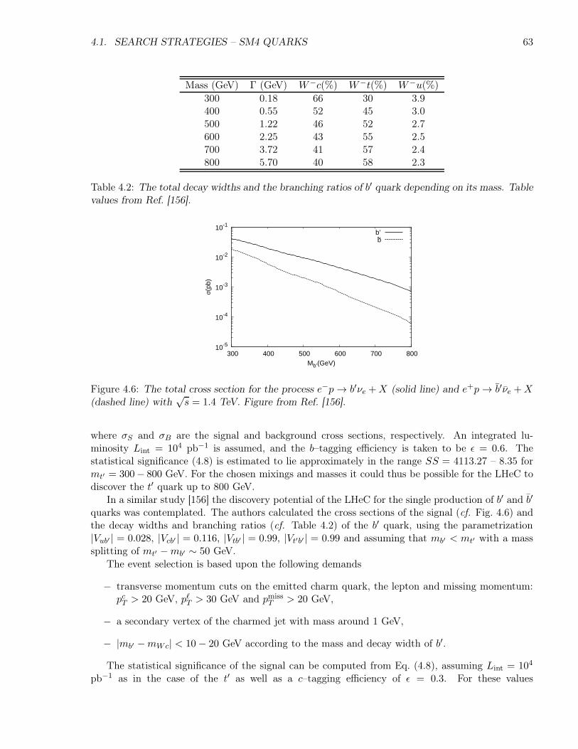
4.1. SEARCH STRATEGIES – SM4 QUARKS 63
Mass (GeV) Γ (GeV) W−c(%) W−t(%) W−u(%)
300 0.18 66 30 3.9400 0.55 52 45 3.0500 1.22 46 52 2.7600 2.25 43 55 2.5700 3.72 41 57 2.4800 5.70 40 58 2.3
Table 4.2: The total decay widths and the branching ratios of b′ quark depending on its mass. Tablevalues from Ref. [156].
10-5
10-4
10-3
10-2
10-1
300 400 500 600 700 800
σ(pb
)
Mb’(GeV)
b’b-’
Figure 4.6: The total cross section for the process e−p→ b′νe +X (solid line) and e+p→ b′νe +X(dashed line) with
√s = 1.4 TeV. Figure from Ref. [156].
where σS and σB are the signal and background cross sections, respectively. An integrated lu-minosity Lint = 104 pb−1 is assumed, and the b–tagging efficiency is taken to be ǫ = 0.6. Thestatistical significance (4.8) is estimated to lie approximately in the range SS = 4113.27 – 8.35 formt′ = 300− 800 GeV. For the chosen mixings and masses it could thus be possible for the LHeC todiscover the t′ quark up to 800 GeV.
In a similar study [156] the discovery potential of the LHeC for the single production of b′ and b′
quarks was contemplated. The authors calculated the cross sections of the signal (cf. Fig. 4.6) andthe decay widths and branching ratios (cf. Table 4.2) of the b′ quark, using the parametrization|Vub′ | = 0.028, |Vcb′ | = 0.116, |Vtb′ | = 0.99, |Vt′b′ | = 0.99 and assuming that mb′ < mt′ with a masssplitting of mt′ −mb′ ∼ 50 GeV.
The event selection is based upon the following demands
− transverse momentum cuts on the emitted charm quark, the lepton and missing momentum:pcT > 20 GeV, pℓT > 30 GeV and pmiss
T > 20 GeV,
− a secondary vertex of the charmed jet with mass around 1 GeV,
− |mb′ −mWc| < 10− 20 GeV according to the mass and decay width of b′.
The statistical significance of the signal can be computed from Eq. (4.8), assuming Lint = 104
pb−1 as in the case of the t′ as well as a c–tagging efficiency of ǫ = 0.3. For these values
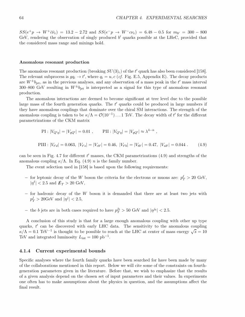
64 CHAPTER 4. EXPERIMENTAL SEARCHES
SS(e+p → W+cνe) = 13.2 − 2.72 and SS(e−p → W−cνe) = 6.48 − 0.5 for mb′ = 300 − 800GeV, rendering the observation of singly produced b′ quarks possible at the LHeC, provided thatthe considered mass range and mixings hold.
Anomalous resonant production
The anomalous resonant production (breaking SU(3)c) of the t′ quark has also been considered [158].The relevant subprocess is gqi → t′, where qi = u, c (cf. Fig. E.5, Appendix E). The decay productsare W±bjet, as in the previous analyses, and any observation of a mass peak in the t′ mass interval300–800 GeV resulting in W±bjet is interpreted as a signal for this type of anomalous resonantproduction.
The anomalous interactions are deemed to become significant at tree level due to the possiblelarge mass of the fourth generation quarks. The t′ quarks could be produced in large numbers ifthey have anomalous couplings that dominate over the chiral SM interactions. The strength of theanomalous coupling is taken to be κ/Λ = O(10−1) . . . 1 TeV. The decay width of t′ for the differentparametrizations of the CKM matrix
PI : |VQ′q| = |VqQ′ | = 0.01 , PII : |VQ′q| = |VqQ′ | ≈ λ4−n ,
PIII : |Vt′d| = 0.063, |Vt′s| = |Vcb′ | = 0.46, |Vt′b| = |Vtb′ | = 0.47, |Vub′ | = 0.044 . (4.9)
can be seen in Fig. 4.7 for different t′ masses, the CKM parametrizations (4.9) and strengths of theanomalous coupling κ/Λ. In Eq. (4.9) n is the family number.
The event selection used in [158] is based upon the following requirements:
− for leptonic decay of the W boson the criteria for the electrons or muons are: pℓT > 20 GeV,|ηℓ| < 2.5 and /ET > 20 GeV,
− for hadronic decay of the W boson it is demanded that there are at least two jets withpjT > 20GeV and |ηj | < 2.5,
− the b jets are in both cases required to have pjbT > 50 GeV and |ηjb | < 2.5.
A conclusion of this study is that for a large enough anomalous coupling with other up typequarks, t′ can be discovered with early LHC data. The sensitivity to the anomalous couplingκ/Λ = 0.1 TeV−1 is thought to be possible to reach at the LHC at center of mass energy
√s = 10
TeV and integrated luminosity Lint = 100 pb−1.
4.1.4 Current experimental bounds
Specific analyses where the fourth family quarks have been searched for have been made by manyof the collaborations mentioned in this report. Below we will cite some of the constraints on fourth-generation parameters given in the literature. Before that, we wish to emphasize that the resultsof a given analysis depend on the chosen set of input parameters and their values. In experimentsone often has to make assumptions about the physics in question, and the assumptions affect thefinal result.
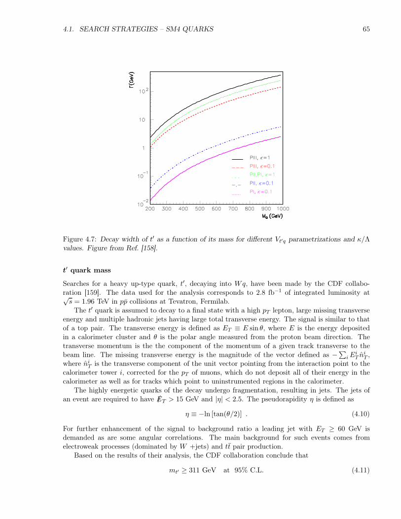
4.1. SEARCH STRATEGIES – SM4 QUARKS 65
Figure 4.7: Decay width of t′ as a function of its mass for different Vt′q parametrizations and κ/Λvalues. Figure from Ref. [158].
t′ quark mass
Searches for a heavy up-type quark, t′, decaying into Wq, have been made by the CDF collabo-ration [159]. The data used for the analysis corresponds to 2.8 fb−1 of integrated luminosity at√s = 1.96 TeV in pp collisions at Tevatron, Fermilab.
The t′ quark is assumed to decay to a final state with a high pT lepton, large missing transverseenergy and multiple hadronic jets having large total transverse energy. The signal is similar to thatof a top pair. The transverse energy is defined as ET ≡ E sin θ, where E is the energy depositedin a calorimeter cluster and θ is the polar angle measured from the proton beam direction. Thetransverse momentum is the the component of the momentum of a given track transverse to thebeam line. The missing transverse energy is the magnitude of the vector defined as −∑iE
iT n
iT ,
where niT is the transverse component of the unit vector pointing from the interaction point to thecalorimeter tower i, corrected for the pT of muons, which do not deposit all of their energy in thecalorimeter as well as for tracks which point to uninstrumented regions in the calorimeter.
The highly energetic quarks of the decay undergo fragmentation, resulting in jets. The jets ofan event are required to have /ET > 15 GeV and |η| < 2.5. The pseudorapidity η is defined as
η ≡ −ln [tan(θ/2)] . (4.10)
For further enhancement of the signal to background ratio a leading jet with ET ≥ 60 GeV isdemanded as are some angular correlations. The main background for such events comes fromelectroweak processes (dominated by W +jets) and tt pair production.
Based on the results of their analysis, the CDF collaboration conclude that
mt′ ≥ 311 GeV at 95% C.L. (4.11)

66 CHAPTER 4. EXPERIMENTAL SEARCHES
The authors note that this result is deduced assuming that the true top mass is 175 GeV but thatthe top quark mass may have been affected by the presence of a heavier t′ and that the conclusionshould the treated with care.
If the fourth generation quarks dominantly mix with the first two generations then t′ and b′ willhave the same signature and the Tevatron observation limit is raised to well over 400 GeV [155] andon the other hand, if a more general, wide range of mixings are considered, a reinterpretation of theCDF results give a lower bound of mt′ &290 GeV [160].
These results have since been improved by the CMS collaboration [161, 162], reporting
mt′ ≥ 450 GeV (semileptonic channel) ,
mt′ ≥ 557 GeV (dilepton channel) . (4.12)
b′ quark mass
CDF has also performed searches for new particles decaying into a Z boson and jets [163], signalinga b′ quark. The data sample used has a luminosity of 1.06 fb−1, collected using Z → ee and Z → µµ.It is assumed that the production mechanisms of the b′ quark would be identical to that of the top,with pair production having the largest cross section. An assumption used for the analysis is thatthe branching ratio of b′ to a Z and a b is 100%.
The main background for such a final state is from SM Z production with jets produced inhigher order QCD processes 1. The optimal kinetic region of the four–generation model drives thefocus of the searches to final states with at least 3 jets, each with a transverse energy ET > 30GeV. Topologies with large numbers of highly energetic jets in the final state allow for a betterseparation of the signal from the standard model Z+jet background, since the generic behavior ofnew signals is that the cross section decreases and the transverse energy spectra become harder asmass increases.
The result of the analysis [163], that mb′ ≥ 268 GeV at 95 % C.L., has been superseded byATLAS [164] and CMS [165] in 2012, reporting
mb′ ≥ 480 GeV and mb′ ≥ 611 GeV , (4.13)
respectively.
4.2 Searches for fourth generation leptons
Pair production of fourth generation leptons
As discussed in Section 2.5.2, neutrinos can have either a Dirac or a Majorana mass – in the mostgeneral case both components are present. The main difference in the pair production of Dirac vs.Majorana neutrinos is the dependence of the cross section on the velocity β. In the case of a Diracmass the cross section has a β–dependence ∼ β(3− β2) while in the Majorana case there is only aterm ∼ β3, implying that the threshold cross section falls more rapidly in the Majorana case as inthe Dirac case. [166]
1Other sources of background may be [163]:– single-Z production in conjunction with jets – ZZ+jets, where one of the Z’s decays to jets– multi-jet events, where two jets fake leptons – WW+jets, where both W ’s decay to leptons– cosmic rays coincident with multi-jet events – tt+jets– WZ+jets, where the W decays to jets.
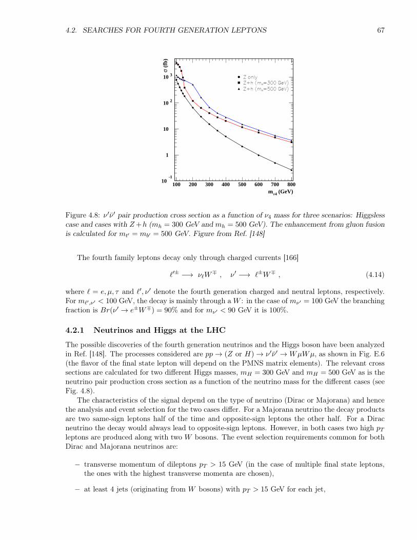
4.2. SEARCHES FOR FOURTH GENERATION LEPTONS 67
10-1
1
10
10 2
10 3
100 200 300 400 500 600 700 800mν4 (GeV)
σ (f
b)
Figure 4.8: ν ′ν ′ pair production cross section as a function of ν4 mass for three scenarios: Higgslesscase and cases with Z+h (mh = 300 GeV and mh = 500 GeV). The enhancement from gluon fusionis calculated for mt′ = mb′ = 500 GeV. Figure from Ref. [148]
The fourth family leptons decay only through charged currents [166]
ℓ′± −→ νℓW∓ , ν ′ −→ ℓ±W∓ , (4.14)
where ℓ = e, µ, τ and ℓ′, ν ′ denote the fourth generation charged and neutral leptons, respectively.For mℓ′,ν′ < 100 GeV, the decay is mainly through a W : in the case of mν′ = 100 GeV the branchingfraction is Br(ν ′ → e±W∓) = 90% and for mν′ < 90 GeV it is 100%.
4.2.1 Neutrinos and Higgs at the LHC
The possible discoveries of the fourth generation neutrinos and the Higgs boson have been analyzedin Ref. [148]. The processes considered are pp→ (Z or H) → ν ′ν ′ →WµWµ, as shown in Fig. E.6(the flavor of the final state lepton will depend on the PMNS matrix elements). The relevant crosssections are calculated for two different Higgs masses, mH = 300 GeV and mH = 500 GeV as is theneutrino pair production cross section as a function of the neutrino mass for the different cases (seeFig. 4.8).
The characteristics of the signal depend on the type of neutrino (Dirac or Majorana) and hencethe analysis and event selection for the two cases differ. For a Majorana neutrino the decay productsare two same-sign leptons half of the time and opposite-sign leptons the other half. For a Diracneutrino the decay would always lead to opposite-sign leptons. However, in both cases two high pTleptons are produced along with two W bosons. The event selection requirements common for bothDirac and Majorana neutrinos are:
− transverse momentum of dileptons pT > 15 GeV (in the case of multiple final state leptons,the ones with the highest transverse momenta are chosen),
− at least 4 jets (originating from W bosons) with pT > 15 GeV for each jet,
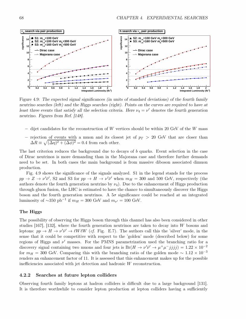
68 CHAPTER 4. EXPERIMENTAL SEARCHES
)-1Integrated Luminosity (fb0 0.2 0.4 0.6 0.8 1 1.2 1.4 1.6 1.8 2
sign
ifica
nce
0
2
4
6
8
10
12
14
search via pair production 4
ν
=100 GeV4νS1: m
=300 GeVh
=100 GeV m4νS2: m
=500 GeVh
=160 GeV m4νS3: m
Dirac caseMajorana case
search via pair production 4
ν
)-1Integrated Luminosity (fb0 0.2 0.4 0.6 0.8 1 1.2 1.4 1.6 1.8 2
sign
ifica
nce
0
2
4
6
8
10
12
14
pair production 4
νh search via
=300 GeVh
=100 GeV m4νS2: m
=500 GeVh
=160 GeV m4νS3: m
Dirac caseMajorana case
pair production 4
νh search via
Figure 4.9: The expected signal significances (in units of standard deviations) of the fourth familyneutrino searches (left) and the Higgs searches (right). Points on the curves are required to have atleast three events that satisfy all the selection criteria. Here ν4 = ν ′ denotes the fourth generationneutrino. Figures from Ref. [148].
− dijet candidates for the reconstruction of W vertices should be within 20 GeV of the W mass
− rejection of events with a muon and its closest jet of pT > 20 GeV that are closer than∆R ≡
√(∆η)2 + (∆φ)2 = 0.4 from each other.
The last criterion reduces the background due to decays of b quarks. Event selection in the caseof Dirac neutrinos is more demanding than in the Majorana case and therefore further demandsneed to be set. In both cases the main background is from massive diboson associated dimuonproduction.
Fig. 4.9 shows the significance of the signals analyzed. S1 in the legend stands for the processpp → Z → ν ′ν ′, S2 and S3 for pp → H → ν ′ν ′ when mH = 300 and 500 GeV, respectively (theauthors denote the fourth generation neutrino by ν4). Due to the enhancement of Higgs productionthrough gluon fusion, the LHC is estimated to have the chance to simultaneously discover the Higgsboson and the fourth generation neutrinos. A 5σ significance could be reached at an integratedluminosity of ∼350 pb−1 if mH = 300 GeV and mν′ = 100 GeV.
The Higgs
The possibility of observing the Higgs boson through this channel has also been considered in otherstudies [167], [132], where the fourth generation neutrinos are taken to decay into W bosons andleptons: pp → H → ν ′ν ′ → ℓWℓW (cf. Fig. E.7). The authors call this the ’silver’ mode, in thesense that it could be competitive with respect to the ’golden’ mode (described below) for someregions of Higgs and ν ′ masses. For the PMNS parametrization used the branching ratio for adiscovery signal containing two muons and four jets is Br(H → ν ′ν ′ → µ+µ−jjjj) = 1.22 × 10⁻²
for mH = 300 GeV. Comparing this with the branching ratio of the golden mode ∼ 1.12 × 10⁻³
renders an enhancement factor of 11. It is assessed that this enhancement makes up for the possibleinefficiencies associated with jet detection and hadronic W reconstruction.
4.2.2 Searches at future lepton colliders
Observing fourth family leptons at hadron colliders is difficult due to a large background [131].It is therefore worthwhile to consider lepton production at lepton colliders having a sufficiently
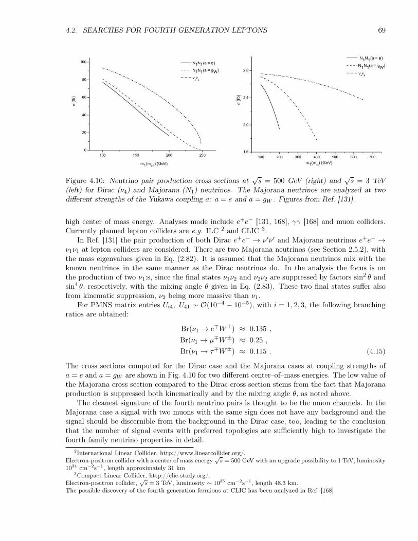
4.2. SEARCHES FOR FOURTH GENERATION LEPTONS 69
Figure 4.10: Neutrino pair production cross sections at√s = 500 GeV (right) and
√s = 3 TeV
(left) for Dirac (ν4) and Majorana (N1) neutrinos. The Majorana neutrinos are analyzed at twodifferent strengths of the Yukawa coupling a: a = e and a = gW . Figures from Ref. [131].
high center of mass energy. Analyses made include e+e− [131, 168], γγ [168] and muon colliders.Currently planned lepton colliders are e.g. ILC 2 and CLIC 3.
In Ref. [131] the pair production of both Dirac e+e− → ν ′ν ′ and Majorana neutrinos e+e− →ν1ν1 at lepton colliders are considered. There are two Majorana neutrinos (see Section 2.5.2), withthe mass eigenvalues given in Eq. (2.82). It is assumed that the Majorana neutrinos mix with theknown neutrinos in the same manner as the Dirac neutrinos do. In the analysis the focus is onthe production of two ν1:s, since the final states ν1ν2 and ν2ν2 are suppressed by factors sin2 θ andsin4 θ, respectively, with the mixing angle θ given in Eq. (2.83). These two final states suffer alsofrom kinematic suppression, ν2 being more massive than ν1.
For PMNS matrix entries Ui4, U41 ∼ O(10−4 − 10−5), with i = 1, 2, 3, the following branchingratios are obtained:
Br(ν1 → e∓W±) ≈ 0.135 ,
Br(ν1 → µ∓W±) ≈ 0.25 ,
Br(ν1 → τ∓W±) ≈ 0.115 . (4.15)
The cross sections computed for the Dirac case and the Majorana cases at coupling strengths ofa = e and a = gW are shown in Fig. 4.10 for two different center–of–mass energies. The low value ofthe Majorana cross section compared to the Dirac cross section stems from the fact that Majoranaproduction is suppressed both kinematically and by the mixing angle θ, as noted above.
The cleanest signature of the fourth neutrino pairs is thought to be the muon channels. In theMajorana case a signal with two muons with the same sign does not have any background and thesignal should be discernible from the background in the Dirac case, too, leading to the conclusionthat the number of signal events with preferred topologies are sufficiently high to investigate thefourth family neutrino properties in detail.
2International Linear Collider, http://www.linearcollider.org/.Electron-positron collider with a center of mass energy
√s = 500 GeV with an upgrade possibility to 1 TeV, luminosity
1034 cm−2s−1, length approximately 31 km3Compact Linear Collider, http://clic-study.org/.
Electron-positron collider,√s = 3 TeV, luminosity ∼ 10
35 cm−2s−1, length 48.3 km.The possible discovery of the fourth generation fermions at CLIC has been analyzed in Ref. [168]
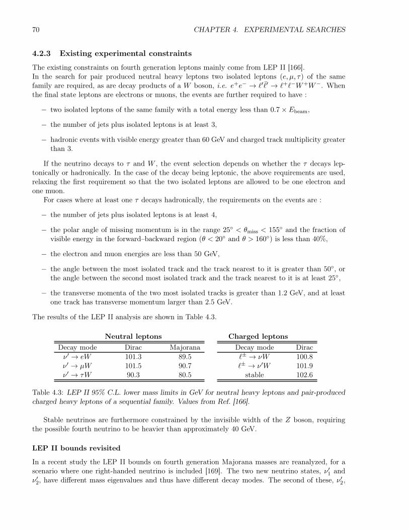
70 CHAPTER 4. EXPERIMENTAL SEARCHES
4.2.3 Existing experimental constraints
The existing constraints on fourth generation leptons mainly come from LEP II [166].In the search for pair produced neutral heavy leptons two isolated leptons (e, µ, τ) of the samefamily are required, as are decay products of a W boson, i.e. e+e− → ℓ′ℓ′ → ℓ+ℓ−W+W−. Whenthe final state leptons are electrons or muons, the events are further required to have :
− two isolated leptons of the same family with a total energy less than 0.7× Ebeam,
− the number of jets plus isolated leptons is at least 3,
− hadronic events with visible energy greater than 60 GeV and charged track multiplicity greaterthan 3.
If the neutrino decays to τ and W , the event selection depends on whether the τ decays lep-tonically or hadronically. In the case of the decay being leptonic, the above requirements are used,relaxing the first requirement so that the two isolated leptons are allowed to be one electron andone muon.
For cases where at least one τ decays hadronically, the requirements on the events are :
− the number of jets plus isolated leptons is at least 4,
− the polar angle of missing momentum is in the range 25 < θmiss < 155 and the fraction ofvisible energy in the forward–backward region (θ < 20 and θ > 160) is less than 40%,
− the electron and muon energies are less than 50 GeV,
− the angle between the most isolated track and the track nearest to it is greater than 50, orthe angle between the second most isolated track and the track nearest to it is at least 25,
− the transverse momenta of the two most isolated tracks is greater than 1.2 GeV, and at leastone track has transverse momentum larger than 2.5 GeV.
The results of the LEP II analysis are shown in Table 4.3.
Neutral leptons
Decay mode Dirac Majorana
ν ′ → eW 101.3 89.5ν ′ → µW 101.5 90.7ν ′ → τW 90.3 80.5
Charged leptons
Decay mode Dirac
ℓ± → νW 100.8ℓ± → ν ′W 101.9
stable 102.6
Table 4.3: LEP II 95% C.L. lower mass limits in GeV for neutral heavy leptons and pair-producedcharged heavy leptons of a sequential family. Values from Ref. [166].
Stable neutrinos are furthermore constrained by the invisible width of the Z boson, requiringthe possible fourth neutrino to be heavier than approximately 40 GeV.
LEP II bounds revisited
In a recent study the LEP II bounds on fourth generation Majorana masses are reanalyzed, for ascenario where one right-handed neutrino is included [169]. The two new neutrino states, ν ′1 andν ′2, have different mass eigenvalues and thus have different decay modes. The second of these, ν ′2,

4.3. HIGGS SEARCHES 71
ν ′1 decay mode Bounds
Wτ 62.1Wµ 79.9We 81.8
Table 4.4: Bounds on ν ′1 mass in GeV for the various decay channels. Values from Ref. [169].
is by assumption heavy (mν′2> mν′
1) and can decay either into ℓW , with ℓ = e, µ, τ or into ν ′1Z.
The first of these modes is suppressed by the small mixing between the fourth generation with theothers and the second mode dominates for most masses. For the lighter neutrino the only openchannel is ν ′1 → ℓW .
The relative branching ratios of the channels depend on the unknown PMNS matrix elements. Inthe limit of complete mass degeneracy (pseudo-Dirac limit), there is phase space suppression of thefirst decay mode of ν ′2 and there may be model-dependent interference effects and other effects likedisplaced vertices. Therefore the authors have chosen to restrict their analysis to mass differencesgreater than 10 GeV. The results of the study are shown in Table 4.4. We see that the the LEP IIbounds 4.3 are altered significantly.
A conclusion drawn is that if a fourth generation exists, relatively light right-handed neutrinosmust exist in order to generate a sufficiently large neutrino mass and that the existence of theseextra states modifies the search strategies for the fourth generation lepton sector.
4.3 Higgs searches
4.3.1 Higgs searches at Tevatron
A study made about ten years ago focused on the discovery of the Higgs boson at the upgradedTevatron, taking into account the four–family model [170]. For a Higgs boson with mass in therange 175 < mH < 300 GeV, the ‘golden’ mode H → ZZ → 4ℓ (cf. Fig. E.7, Appendix E) is themost reliable one for the possible discovery of the Higgs boson. The discovery potential dependsmainly on the available integrated luminosity. The cross section for this process depends on theHiggs boson mass, as shown in Fig. 4.11.
The main background from the pair production of Z bosons, namely pp → ZZX, such thatZ → ℓ+ℓ− is reduced by the reconstruction of the four-lepton invariant mass distribution. Thismode is thus esteemed to allow for :
Tevatron > 3σ observation of the Higgs possible for 175 < mSM4H < 300 GeV. (4.16)
Recently the Tevatron experiments CDF and D/0 have updated their analyses using data of 8.2fb−1 from CDF and 8.1 fb−1 from D/0 [171]. The collaborations searched for the Higgs boson in thedecays H →W+W− and H → ZZ, using all the production processes of the SM, namely gg → H,qq →WH, qq → ZH and vector boson fusion.
Two four–generation scenarios are considered: a ‘low–mass’ scenario and a ‘high–mass’ scenario(see Fig. 4.12). In the former the authors fix the masses of the fourth generation leptons at mν′ = 80GeV and mℓ′ = 100 GeV, in order to have maximum impact on Higgs decay ratios but to evadecurrent experimental limits; in the latter they set mν′ = mℓ′ = 1 TeV, in which case the leptons ofthe fourth generation do not affect the branching ratios at all (they are kinematically inaccessible).
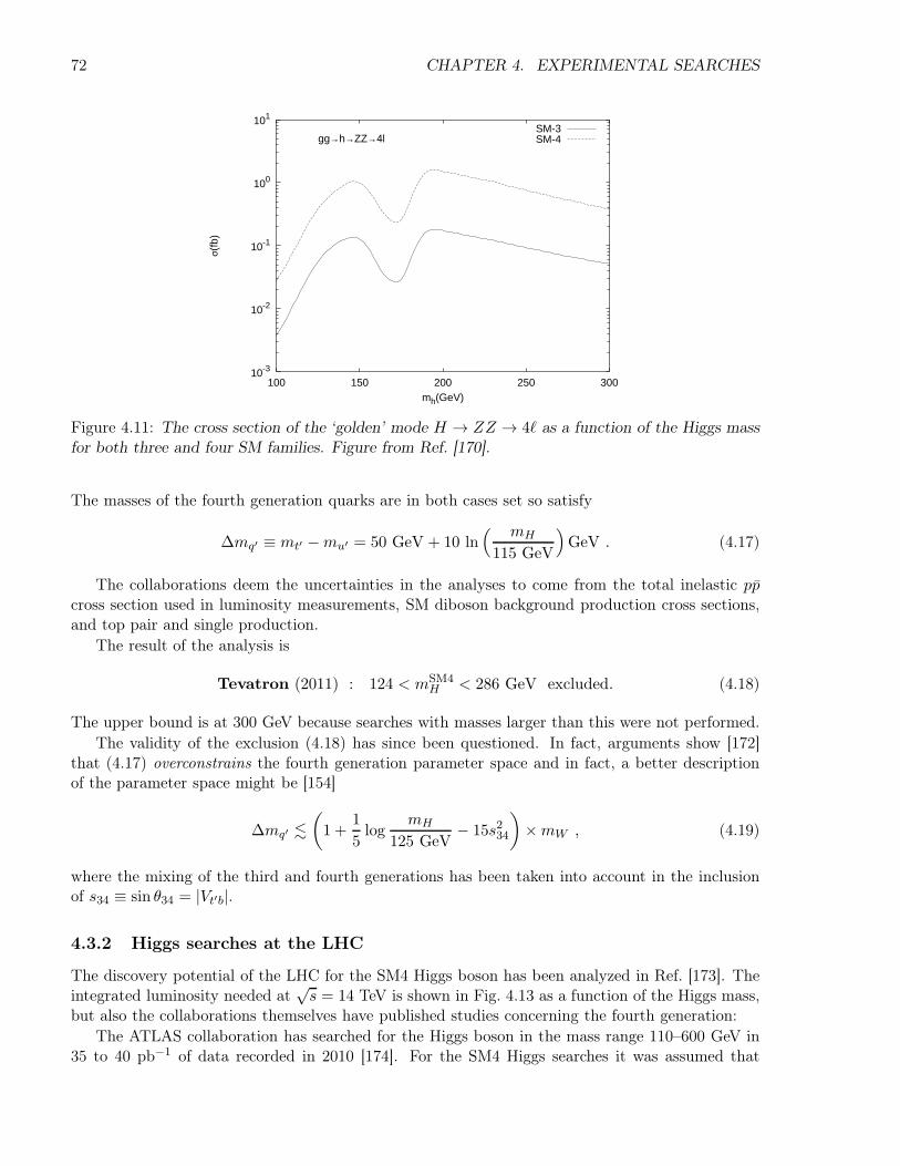
72 CHAPTER 4. EXPERIMENTAL SEARCHES
10-3
10-2
10-1
100
101
100 150 200 250 300
σ(fb
)
mh(GeV)
gg→h→ZZ→4lSM-3SM-4
Figure 4.11: The cross section of the ‘golden’ mode H → ZZ → 4ℓ as a function of the Higgs massfor both three and four SM families. Figure from Ref. [170].
The masses of the fourth generation quarks are in both cases set so satisfy
∆mq′ ≡ mt′ −mu′ = 50 GeV + 10 ln( mH
115 GeV
)GeV . (4.17)
The collaborations deem the uncertainties in the analyses to come from the total inelastic ppcross section used in luminosity measurements, SM diboson background production cross sections,and top pair and single production.
The result of the analysis is
Tevatron (2011) : 124 < mSM4H < 286 GeV excluded. (4.18)
The upper bound is at 300 GeV because searches with masses larger than this were not performed.
The validity of the exclusion (4.18) has since been questioned. In fact, arguments show [172]that (4.17) overconstrains the fourth generation parameter space and in fact, a better descriptionof the parameter space might be [154]
∆mq′ .
(1 +
1
5log
mH
125 GeV− 15s234
)×mW , (4.19)
where the mixing of the third and fourth generations has been taken into account in the inclusionof s34 ≡ sin θ34 = |Vt′b|.
4.3.2 Higgs searches at the LHC
The discovery potential of the LHC for the SM4 Higgs boson has been analyzed in Ref. [173]. Theintegrated luminosity needed at
√s = 14 TeV is shown in Fig. 4.13 as a function of the Higgs mass,
but also the collaborations themselves have published studies concerning the fourth generation:
The ATLAS collaboration has searched for the Higgs boson in the mass range 110–600 GeV in35 to 40 pb−1 of data recorded in 2010 [174]. For the SM4 Higgs searches it was assumed that
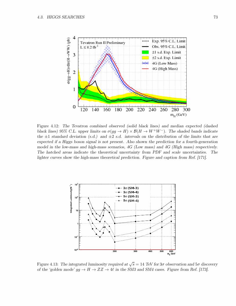
4.3. HIGGS SEARCHES 73
Figure 4.12: The Tevatron combined observed (solid black lines) and median expected (dashedblack lines) 95% C.L. upper limits on σ(gg → H) × B(H → W+W−). The shaded bands indicatethe ±1 standard deviation (s.d.) and ±2 s.d. intervals on the distribution of the limits that areexpected if a Higgs boson signal is not present. Also shown the prediction for a fourth-generationmodel in the low-mass and high-mass scenarios, 4G (Low mass) and 4G (High mass) respectively.The hatched areas indicate the theoretical uncertainty from PDF and scale uncertainties. Thelighter curves show the high-mass theoretical prediction. Figure and caption from Ref. [171].
Figure 4.13: The integrated luminosity required at√s = 14 TeV for 3σ observation and 5σ discovery
of the ‘golden mode’ gg → H → ZZ → 4ℓ in the SM3 and SM4 cases. Figure from Ref. [173].
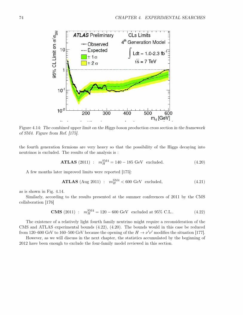
74 CHAPTER 4. EXPERIMENTAL SEARCHES
Figure 4.14: The combined upper limit on the Higgs boson production cross section in the frameworkof SM4. Figure from Ref. [175].
the fourth generation fermions are very heavy so that the possibility of the Higgs decaying intoneutrinos is excluded. The results of the analysis is :
ATLAS (2011) : mSM4H = 140 − 185 GeV excluded. (4.20)
A few months later improved limits were reported [175]:
ATLAS (Aug 2011) : mSM4H < 600 GeV excluded, (4.21)
as is shown in Fig. 4.14.Similarly, according to the results presented at the summer conferences of 2011 by the CMS
collaboration [176]
CMS (2011) : mSM4H = 120 − 600 GeV excluded at 95% C.L.. (4.22)
The existence of a relatively light fourth family neutrino might require a reconsideration of theCMS and ATLAS experimental bounds (4.22), (4.20). The bounds would in this case be reducedfrom 120–600 GeV to 160–500 GeV because the opening of the H → ν ′ν ′ modifies the situation [177].
However, as we will discuss in the next chapter, the statistics accumulated by the beginning of2012 have been enough to exclude the four-family model reviewed in this section.
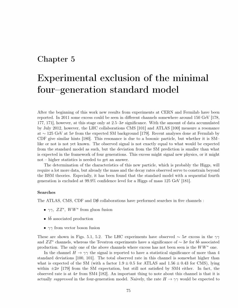
Chapter 5
Experimental exclusion of the minimal
four–generation standard model
After the beginning of this work new results from experiments at CERN and Fermilab have beenreported. In 2011 some excess could be seen in different channels somewhere around 150 GeV [178,177, 171], however, at this stage only at 2.5–3σ significance. With the amount of data accumulatedby July 2012, however, the LHC collaborations CMS [101] and ATLAS [100] measure a resonanceat ∼ 125 GeV at 5σ from the expected SM background [179]. Recent analyses done at Fermilab byCDF give similar hints [180]. This resonance is due to a bosonic particle, but whether it is SM–like or not is not yet known. The observed signal is not exactly equal to what would be expectedfrom the standard model as such, but the deviation from the SM prediction is smaller than whatis expected in the framework of four generations. This excess might signal new physics, or it mightnot – higher statistics is needed to get an answer.
The determination of the characteristics of this new particle, which is probably the Higgs, willrequire a lot more data, but already the mass and the decay rates observed serve to constrain beyondthe BSM theories. Especially, it has been found that the standard model with a sequential fourthgeneration is excluded at 99.9% confidence level for a Higgs of mass 125 GeV [181].
Searches
The ATLAS, CMS, CDF and D/0 collaborations have performed searches in five channels :
• γγ, ZZ∗, WW ∗ from gluon fusion
• bb associated production
• γγ from vector boson fusion
These are shown in Figs. 5.1, 5.2. The LHC experiments have observed ∼ 5σ excess in the γγand ZZ∗ channels, whereas the Tevatron experiments have a significance of ∼ 3σ for bb associatedproduction. The only one of the above channels where excess has not been seen is the WW ∗ one.
In the channel H → γγ the signal is reported to have a statistical significance of more than 4standard deviations [100, 101]. The total observed rate in this channel is somewhat higher thanwhat is expected of the SM (with a factor 1.9 ± 0.5 for ATLAS and 1.56 ± 0.43 for CMS), lyingwithin ±2σ [179] from the SM expectation, but still not satisfied by SM4 either. In fact, theobserved rate is at 4σ from SM4 [182]. An important thing to note about this channel is that it isactually suppressed in the four-generation model. Naively, the rate H → γγ would be expected to
75
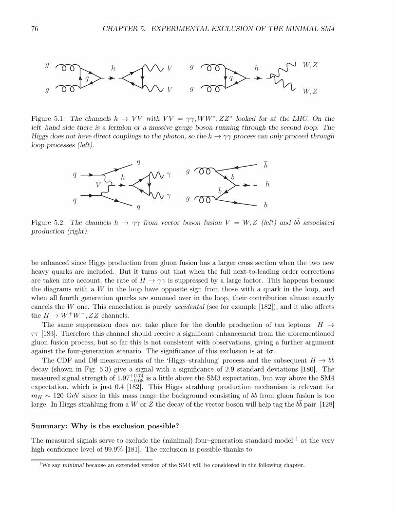
76 CHAPTER 5. EXPERIMENTAL EXCLUSION OF THE MINIMAL SM4
g
g
q
h V
V g
g
qh W,Z
W,Z
Figure 5.1: The channels h → V V with V V = γγ,WW ∗, ZZ∗ looked for at the LHC. On theleft–hand side there is a fermion or a massive gauge boson running through the second loop. TheHiggs does not have direct couplings to the photon, so the h→ γγ process can only proceed throughloop processes (left).
g
gb
b
hb
bγ
γ
hV
q
q
Figure 5.2: The channels h → γγ from vector boson fusion V = W,Z (left) and bb associatedproduction (right).
be enhanced since Higgs production from gluon fusion has a larger cross section when the two newheavy quarks are included. But it turns out that when the full next-to-leading order correctionsare taken into account, the rate of H → γγ is suppressed by a large factor. This happens becausethe diagrams with a W in the loop have opposite sign from those with a quark in the loop, andwhen all fourth generation quarks are summed over in the loop, their contribution almost exactlycancels the W one. This cancelation is purely accidental (see for example [182]), and it also affectsthe H →W+W−, ZZ channels.
The same suppression does not take place for the double production of tau leptons: H →ττ [183]. Therefore this channel should receive a significant enhancement from the aforementionedgluon fusion process, but so far this is not consistent with observations, giving a further argumentagainst the four-generation scenario. The significance of this exclusion is at 4σ.
The CDF and D/0 measurements of the ‘Higgs–strahlung’ process and the subsequent H → bbdecay (shown in Fig. 5.3) give a signal with a significance of 2.9 standard deviations [180]. Themeasured signal strength of 1.97+0.74
−0.68 is a little above the SM3 expectation, but way above the SM4expectation, which is just 0.4 [182]. This Higgs–strahlung production mechanism is relevant formH ∼ 120 GeV since in this mass range the background consisting of bb from gluon fusion is toolarge. In Higgs-strahlung from a W or Z the decay of the vector boson will help tag the bb pair. [128]
Summary: Why is the exclusion possible?
The measured signals serve to exclude the (minimal) four–generation standard model 1 at the veryhigh confidence level of 99.9% [181]. The exclusion is possible thanks to
1We say minimal because an extended version of the SM4 will be considered in the following chapter.

77
q
q
VV
H
b
b
Figure 5.3: The diagram of the ‘Higgs–strahlung’ process with subsequent H → bb decay.
Figure 5.4: Constraints on the SM4 derived from scanning over the fourth generation fermion massesas described in the text. The darker region within the solid borders (light region within the dashedborders) shows the level of exclusion with (without) the γγjj mode. Left: the exclusion limit asa function of the neutrino mass (the other fourth generation fermion masses are scanned) for fixedmh = 125 GeV. Right: the exclusion limit as a function of mh, with all fourth generation massesvaried. Figure and caption from [181].
• gg → h production rate is enhanced by a factor O(10),
• the channel h→ γγ suppressed by a factor O(100),
• at tree level the corrections from the fourth generation to Γ(h → bb) and Γ(h → ZZ∗) aresmall,
• enhancement of H → ττ not seen in experiments
The authors of [181] deduce constraints on the SM4 by minimizing χ2 (A.1) in two differentsettings, depending on the treatment of the mass of the fourth generation neutrino (see Fig. 5.4).They find that for 124 GeV ≤ mh ≤ 127 GeV the SM4 is excluded at a confidence level of morethan 95% and that for the specific mass mh = 125 GeV the exclusion is at 99.9% C.L.
A similar result is obtained in another study, where the authors develop a new method for thecalculation of probabilities in order to evaluate the SM3 and SM4 fits [183]. The new method isnecessary because the SM3 and SM4 are not nested, meaning that the SM3 cannot be obtainedas a special case of SM4 with some parameters fixed. This non–nestedness implies that the usualformulae for computing probabilities in likelihood ratio tests does not work. Hence a new C++framework is developed for this study, where the goodnesses of the SM3 and SM4 fits are evaluated.The χ2–distributions for the two scenarios are shown in Fig. 5.5. The figures show that both in
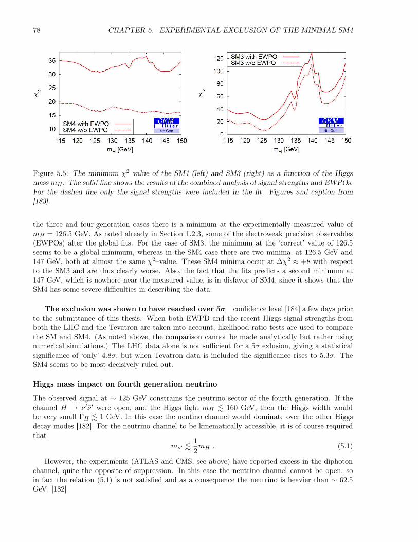
78 CHAPTER 5. EXPERIMENTAL EXCLUSION OF THE MINIMAL SM4
Figure 5.5: The minimum χ2 value of the SM4 (left) and SM3 (right) as a function of the Higgsmass mH . The solid line shows the results of the combined analysis of signal strengths and EWPOs.For the dashed line only the signal strengths were included in the fit. Figures and caption from[183].
the three and four-generation cases there is a minimum at the experimentally measured value ofmH = 126.5 GeV. As noted already in Section 1.2.3, some of the electroweak precision observables(EWPOs) alter the global fits. For the case of SM3, the minimum at the ‘correct’ value of 126.5seems to be a global minimum, whereas in the SM4 case there are two minima, at 126.5 GeV and147 GeV, both at almost the same χ2–value. These SM4 minima occur at ∆χ2 ≈ +8 with respectto the SM3 and are thus clearly worse. Also, the fact that the fits predicts a second minimum at147 GeV, which is nowhere near the measured value, is in disfavor of SM4, since it shows that theSM4 has some severe difficulties in describing the data.
The exclusion was shown to have reached over 5σ confidence level [184] a few days priorto the submittance of this thesis. When both EWPD and the recent Higgs signal strengths fromboth the LHC and the Tevatron are taken into account, likelihood-ratio tests are used to comparethe SM and SM4. (As noted above, the comparison cannot be made analytically but rather usingnumerical simulations.) The LHC data alone is not sufficient for a 5σ exlusion, giving a statisticalsignificance of ‘only’ 4.8σ, but when Tevatron data is included the significance rises to 5.3σ. TheSM4 seems to be most decisively ruled out.
Higgs mass impact on fourth generation neutrino
The observed signal at ∼ 125 GeV constrains the neutrino sector of the fourth generation. If thechannel H → ν ′ν ′ were open, and the Higgs light mH . 160 GeV, then the Higgs width wouldbe very small ΓH . 1 GeV. In this case the neutino channel would dominate over the other Higgsdecay modes [182]. For the neutrino channel to be kinematically accessible, it is of course requiredthat
mν′ .1
2mH . (5.1)
However, the experiments (ATLAS and CMS, see above) have reported excess in the diphotonchannel, quite the opposite of suppression. In this case the neutrino channel cannot be open, soin fact the relation (5.1) is not satisfied and as a consequence the neutrino is heavier than ∼ 62.5GeV. [182]
Part III
The two Higgs doublet model
79


Chapter 6
Theory of the two Higgs doublet model
After the beginning of this work the minimal four-generation standard model has been excluded byexperiments (see the previous chapter). The use of the word ‘minimal’ here refers to the fact that,in the SM4 we have (as is the case of SM3) just included one Higgs doublet in the scalar sector ofthe theory. It might well be that there exist more than one scalar doublet in nature; at present wedo not know. In the rest of this report we will consider the impact of adding another scalar doubletto the four-generation standard model considered previously.
6.1 Why add another doublet?
In this report we have discussed the number of fermion families in the standard model. An interestingthing to note is that even though we know that there are at least three fermion families and two left–handed SU(2) doublets in each family, the SM still has just one scalar doublet (the ‘standard’ Higgsdoublet). However, there is no reason for there to be just one Higgs doublet, and on the contrarythere are some arguments that favor several such doublets. Motivation for models including twoHiggs doublets (2HDM:s) instead of one include [185]
• Supersymmetry (SUSY)Supersymmetry requires at least two Higgs doublets, because scalars come in chiral multipletsand the complex conjugates come in multiplets of opposite chirality – hence there must be atleast two Higgs doublets.
• Cancellation of anomaliesIn the SM the fermion families need to be complete in order for anomalies to be cancelled.In SUSY, the introduction of a single Higgsino (the supersymmetric partner of the Higgs)introduces anomalies. These are cancelled when one introduces a second doublet.
• Axion modelsAccording to axion models in QCD possible CP violating terms (that are experimentallyknown to be very small) in LQCD may be rotated away if the Lagrangian exhibits a globalU(1) symmetry. Such a symmetry exists only if there are two Higgs doublets.
• Baryon asymmetry of the Universe The baryon asymmetry of the Universe is not properlydescribed by the standard model. 2HDMs, however, may explain this asymmetry thanks tothe flexibility of the scalar mass spectrum as well as additional new sources of CP violation.
81
82 CHAPTER 6. THEORY OF THE 2HDM
A very important parameter giving information about the scalar sector is the ρ parameter (2.62)
ρ =
∑ni=1
Ii(Ii + 1)− 1
4Y2i
vi∑n
i=112Y
2i vi
, (6.1)
whose experimental value is known to be very close to one (2.63). Eq. 6.1 shows that both SU(2)singlets with Y = 0 and doublets with Y = ±1 give ρ = 1 because in both these cases I(I+1) = 3
4Y .
6.2 The scalar potential and the field content
Complex scalar doublets have four degrees of freedom so with two (Higgs) doublets Φ1, Φ2 thereare eight. Three of these are just Goldstone bosons that give masses to the W± and Z and theremaining five are the physical scalars – the Higgs fields. Of these five there is a charged scalar(with two physical states), two neutral ones and a pseudoscalar (see e.g. [128]):
(h0, H0, A0, H±) (6.2)
with masses (mh, mH , mA, m±). Here h0, H0, H± are the scalars (CP–even particles) and A0 isthe pseudoscalar (CP–odd).
Whereas the SM Higgs sector has only one free parameter (the Higgs mass) 2HDMs containseveral free parameters and the vacuum structure is much richer. The most general scalar potentialcontains several parameters and it has CP–conserving, CP–violating and charge–violating minima.The potential reads [185]
V = m211Φ
†1Φ1 +m2
22Φ†2Φ2 −m2
12
(Φ†1Φ2 +Φ†
2Φ1
)+λ12
(Φ†1Φ1
)2+λ22
(Φ†2Φ2
)2
+ λ3Φ†1Φ1 Φ
†2Φ2 + λ4Φ
†1Φ2Φ
†2Φ1 +
λ52
[(Φ†1Φ2
)2+(Φ†2Φ1
)2], (6.3)
for Φ1, Φ2 the two doublets of hypercharge +1. All the parameters of the potential are real. Thelarge Yukawa couplings of the fourth generation fields can destabilize the potential (6.3) due to thepossibly very large radiative corrections that they bring [186]. A way to deal with this problem isto assume that the effective potential of the model is stabilized by some new effect near the TeVscale, and that (6.3) is valid below this scale.
A region of parameter space minimizing the potential (6.3) gives the vacuum expectation values
〈Φ1〉0 =1√2
(0v1
), 〈Φ2〉0 =
1√2
(0v2
). (6.4)
For the vacuum (6.4) the fields have the following mass terms in the Lagrangian
Lmassφ± =
[m2
12 − (λ4 + λ5)v1v2] (
φ−1 , φ−2)
v2v1
−1
−1v1v2
(φ+1φ+2
), (6.5)
Lmassη =
m2A
v21 + v22
(η1, η2
)( v22 −v1v2−v1v2 v21
)(η1η2
), (6.6)
Lmassρ = −
(ρ1, ρ2
)
m212
v2v1
+ λ1v21 −m2
12 + λ345v1v2
−m212 + λ345v1v2 m2
12
v1v2
+ λ2v22
(ρ1ρ2
), (6.7)
6.3. FLAVOR CONSERVATION 83
for λ345 = λ3 + λ4 + λ5 and when the doublet Φi is written
Φi =
φ+i
vi + ρa + iηi√2
, i = 1, 2, (6.8)
with charged scalar φ±, pseudoscalar η and neutral scalar ρ. The mass-squared matrices of Eqs. (6.5),(6.6)each have a zero eigenvalue, corresponding to the massless Goldstones that give the masses to theW± and Z, respectively. Besides the zero eigenvalues these matrices also give the physical massesfor the charged and pseudoscalar Higgses:
m2± = [m2
12/(v1v2)− λ4 − λ5](v21 + v22
)(6.9)
m2A =
[m2
12/(v1v2)− 2λ5] (v21 + v22
)(6.10)
The mass matrices of Eqs. (6.5),(6.6),(6.7) can be diagonalized, but in general not simultaneously.We will discuss this in the next section. Two important parameters in the study of 2HDMs are αand β, the angles that diagonalize the mass–squared matrices of the pseudoscalar and charged scalarsector and the neutral scalar sector, respectively. The angle β is defined using the VEVs of the twodoublets Φ1, Φ2
tan β ≡ v2v1
. (6.11)
6.3 Flavor conservation
As already mentioned, the mass–squared matrices of the various Higgs fields may in general not bediagonalized simultaneously. This gives rise to tree–level flavor–changing neutral currents (FCNC).Since FCNCs have not been observed in nature their existence poses a problem for such modelswith several scalar multiplets. In order to illustrate this let us consider the Lagrangian describingthe mass of down–type quarks [185]
LdY = y
(1)ij ψiψjΦ1 + y
(2)ij ψiψjΦ2, (6.12)
where i, j are a family indices. The corresponding mass matrix reads
Mdij = y
(1)ij
v1√2+ y
(2)ij
v2√2. (6.13)
In the SM, with just one Higgs multiplet, the diagonalization of the mass matrix M implies thediagonalization of the Yukawa couplings y. This is not the case of Eq. (6.13), however, where y(1)
and y(2) usually do not have the same set of eigenvectors,and so in general the Yukawa interactions(6.12) will have FCNCs at the tree level (e.g. couplings dsφ). Getting rid of these is customarilydone by introducing some additional, continuous or discrete symmetries. [185]
There are different ways to introduce the symmetries that hinder the FCNCs. One option is tointroduce a discrete symmetry
Φ1 −→ −Φ1 , (6.14)
which is done for example in the so–called type I 2HDM, where Φ1 is chosen to couple to all fieldsof the theory, and Φ2 to none.
Another option is to have transformations
Φ1 −→ − Φ1 , diR −→ − diR , (6.15)
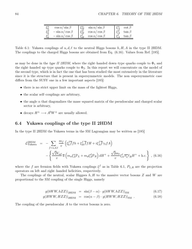
84 CHAPTER 6. THEORY OF THE 2HDM
ξuh cosα/ sin β ξuH sinα/ sin β ξuA cot βξdh − sinα/ cos β ξdH cosα/ cos β ξdA tan βξℓh − sinα/ cos β ξℓH cosα/ cos β ξℓA tan β
Table 6.1: Yukawa couplings of u, d, ℓ to the neutral Higgs bosons h,H,A in the type II 2HDM.The couplings to the charged Higgs bosons are obtained from Eq. (6.16). Values from Ref. [185].
as may be done in the type II 2HDM, where the right–handed down–type quarks couple to Φ1 andthe right–handed up–type quarks couple to Φ2. In this report we will concentrate on the model ofthe second type, which is in fact the one that has been studied the most extensively in the literaturesince it is the structure that is present in supersymmetric models. The non–supersymmetric casediffers from the SUSY one in a few important aspects [185]:
• there is no strict upper limit on the mass of the lightest Higgs,
• the scalar self–couplings are arbitrary,
• the angle α that diagonalizes the mass–squared matrix of the pseudoscalar and charged scalarsector is arbitrary,
• decays H± −→ A0W± are usually allowed.
6.4 Yukawa couplings of the type II 2HDM
In the type II 2HDM the Yukawa terms in the SM Lagrangian may be written as [185]
L2HDMYukawa = −
∑
f=u,d,ℓ
mf
v
(ξfhffh+ ξfHffH + iξfAfγ5fA
)
−√
2Vudv
u(muξ
uAPL +mdξ
dAPR
)dH+ +
√2mℓ
vξℓA νLℓRH
+ + h.c.
, (6.16)
where the f are fermion fields with Yukawa couplings ξf as in Table 6.1, PL,R are the projectionoperators on left and right–handed helicities, respectively.
The couplings of the neutral, scalar Higgses h,H to the massive vector bosons Z and W areproportional to the SM coupling of the single Higgs, namely
g(hWW,hZZ)|2HDM = sin(β − α) · g(hWW,hZZ)|SM (6.17)
g(HWW,HZZ)|2HDM = cos(α− β) · g(HWW,HZZ)|SM . (6.18)
The coupling of the pseudoscalar A to the vector bosons is zero.
Chapter 7
4F2HDM phenomenology
When the second scalar doublet is added to the theory this necessarily affects the production anddecay of the Higgs particles. Already the field content is modified, there are several Higgses, not justone. Also, the couplings of these many scalars are different from the minimal case of the SM. Theproduction and decay probabilities are, as normally done in QFTs, computed from the amplitudes ofthe relevant processes, and these depend on the properties of and the couplings between the fieldsparticipating in the process. What is then experimentally measured in the detectors of particlecolliders are the decay products, and the rates at which different decays are observed. Since thesediffer from model to model the decays, especially through the measured branching ratios, giveinformation about the properties of the decaying particle and allows to distinguish beween variousmodels. That is why we in this section concentrate on the (production and) decay of the fourthgeneration particles and the Higgses of the type–II 2HDM, the model of interest to us.
7.1 Higgs production and decay in the 2HDM–II
An important thing to note about the branching ratios of the extended Higgs sector is that they willnot only depend on the masses but also on the two new parameters α, β that are introduced in thetheory when another scalar doublet is added [128]. Since these two parameters are unknown, theirvalues must be fixed in order to get concrete predictions. This implies that comprehensive analysesare difficult and more specifically that any plot of the branching ratios is necessarily incomplete.
The impact of a fourth generation on SM Higgs production was discussed in Section 3.2. Asnoted before, the dominant production mechanism at hadron colliders is gluon fusion (see Fig. 3.5).In the standard model, the largest contribution comes from a top quark loop, whereas in SM4 thethree heavy quarks t, t′, b′ give the largest contribution. In both these cases the largest contributioncomes from the quarks having the largest Yukawa couplings. Since the bottom quark is quite abit lighter than the top quark, its effect on the gluon fusion process in negligible with respect tothe top. In the four-fermion 2HDM (4F2HDM) model the bottom quark contribution to the loopdiagram 3.5 may for the 2HDM–II be sizeable and even dominate over t in a region of parameterspace.
As the Yukawa couplings of the various Higgses differ, we will present their production anddecays separately. We will only consider the two lightest particles h0 and A0 since these are theones that are most likely to be discovered at particle colliders, and h0 has perhaps already beenfound (see Chapter 5).
85
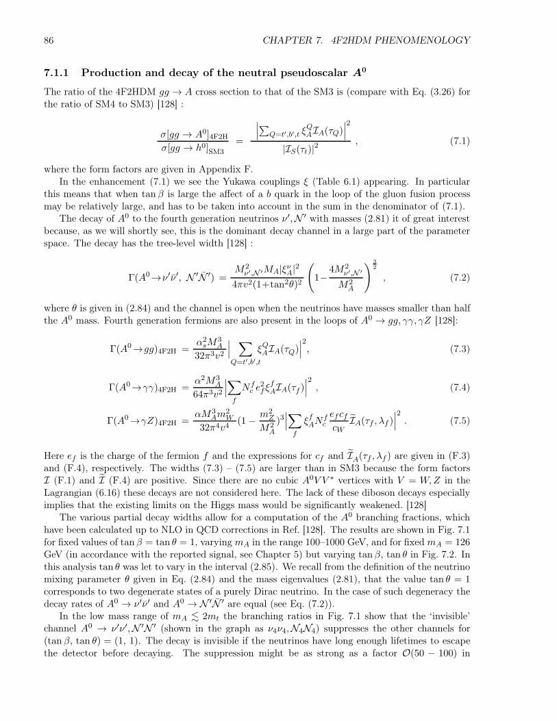
86 CHAPTER 7. 4F2HDM PHENOMENOLOGY
7.1.1 Production and decay of the neutral pseudoscalar A0
The ratio of the 4F2HDM gg → A cross section to that of the SM3 is (compare with Eq. (3.26) forthe ratio of SM4 to SM3) [128] :
σ[gg → A0]4F2Hσ[gg → h0]SM3
=
∣∣∣∑
Q=t′,b′,t ξQAIA(τQ)
∣∣∣2
|IS(τt)|2, (7.1)
where the form factors are given in Appendix F.In the enhancement (7.1) we see the Yukawa couplings ξ (Table 6.1) appearing. In particular
this means that when tan β is large the affect of a b quark in the loop of the gluon fusion processmay be relatively large, and has to be taken into account in the sum in the denominator of (7.1).
The decay of A0 to the fourth generation neutrinos ν ′,N ′ with masses (2.81) it of great interestbecause, as we will shortly see, this is the dominant decay channel in a large part of the parameterspace. The decay has the tree-level width [128] :
Γ(A0→ν ′ν ′, N ′N ′) =M2
ν′,N ′MA|ξνA|24πv2(1+tan2θ)2
(1−
4M2ν′,N ′
M2A
) 3
2
, (7.2)
where θ is given in (2.84) and the channel is open when the neutrinos have masses smaller than halfthe A0 mass. Fourth generation fermions are also present in the loops of A0 → gg, γγ, γZ [128]:
Γ(A0→gg)4F2H =α2sM
3A
32π3v2
∣∣∣∑
Q=t′,b′,t
ξQAIA(τQ)∣∣∣2, (7.3)
Γ(A0→γγ)4F2H =α2M3
A
64π3v2
∣∣∣∑
f
Nfc e
2f ξ
fAIA(τf )
∣∣∣2, (7.4)
Γ(A0→γZ)4F2H =αM3
Am2W
32π4v4(1− m2
Z
M2A
)3∣∣∣∑
f
ξfANfc
ef cfcW
IA(τf , λf )∣∣∣2. (7.5)
Here ef is the charge of the fermion f and the expressions for cf and IA(τf , λf ) are given in (F.3)and (F.4), respectively. The widths (7.3) – (7.5) are larger than in SM3 because the form factorsI (F.1) and I (F.4) are positive. Since there are no cubic A0V V ∗ vertices with V = W,Z in theLagrangian (6.16) these decays are not considered here. The lack of these diboson decays especiallyimplies that the existing limits on the Higgs mass would be significantly weakened. [128]
The various partial decay widths allow for a computation of the A0 branching fractions, whichhave been calculated up to NLO in QCD corrections in Ref. [128]. The results are shown in Fig. 7.1for fixed values of tan β = tan θ = 1, varying mA in the range 100–1000 GeV, and for fixed mA = 126GeV (in accordance with the reported signal, see Chapter 5) but varying tan β, tan θ in Fig. 7.2. Inthis analysis tan θ was let to vary in the interval (2.85). We recall from the definition of the neutrinomixing parameter θ given in Eq. (2.84) and the mass eigenvalues (2.81), that the value tan θ = 1corresponds to two degenerate states of a purely Dirac neutrino. In the case of such degeneracy thedecay rates of A0 → ν ′ν ′ and A0 → N ′N ′ are equal (see Eq. (7.2)).
In the low mass range of mA . 2mt the branching ratios in Fig. 7.1 show that the ‘invisible’channel A0 → ν ′ν ′,N ′N ′ (shown in the graph as ν4ν4,N4N4) suppresses the other channels for(tan β, tan θ) = (1, 1). The decay is invisible if the neutrinos have long enough lifetimes to escapethe detector before decaying. The suppression might be as strong as a factor O(50 − 100) in

7.1. HIGGS PRODUCTION AND DECAY IN THE 2HDM–II 87
Figure 7.1: Decay branching ratios of the CP-odd Higgs boson A0 as functions of its mass MA
for the 4F2HDM-II. The other input parameters are fixed as (tan β, tan θ) = (1, 1). Figure andcaption from [128].
Figure 7.2: Decay branching ratios of the CP-odd Higgs boson A0 with mass MA = 126GeV forthe 4F2HDM-II. Plot-(a): Br
[A0]
as a function of the fourth-family neutrino mixing angle tan θ,with fixed tan β = 1. Plot-(b): Br
[A0]
as a function of tan β, with fixed tan θ = 1. Figure andcaption from [128].

88 CHAPTER 7. 4F2HDM PHENOMENOLOGY
comparison to BR(H → γγ) of SM3 [128]. This invisible channel seems to be dominant at all valuesof tan θ considered as well as for moderate values tan β . 2. Therefore the diphoton channel is thegood one for discovery in the light-mass range, the range in which a new particle has recently beenseen (see Chapter 5). The type-II 2HDM with four generations can explain the observed excess inthis signal. The lack of A0V V ∗ vertices implying the lack of significant BR(A0 → V V ∗) is also inaccordance with the data, lacking a signal in the H →WW ∗ channel. [128]
7.1.2 Production and decay of the light neutral Higgs h0
The case of the light, neutral scalar is more complicated than the previous considerations, becauseh0 mixes with the other neutral scalar, the heavier H0. Hence there is one more free parameter, andthat is the h0 −H0 mixing angle α. There are also two more tree-level decay channels to consider,namely the ones into the massive gauge bosons, since h0 has couplings h0V V ∗ (where V = W,Z)of strength (6.17).
As in the case of A0 also h0 production is enhanced by the fourth generation quarks, which haveYukawa couplings as given in the first row of Table 6.1. For a SM Higgs of the mass of h0, the ratioof the 4F2HDM gluon fusion cross section to that of the SM3 has an expression analogous to thatof Eq. (7.1) in the case of the pseudoscalar [128]:
σ[gg → h0]4F2Hσ[gg → h0]SM3
=
∣∣∣∑
Q=t′,b′,t ξQh IS(τQ)
∣∣∣2
|IS(τt)|2, (7.6)
The ratio (7.6) is moderate due to the couplings ξh (Table 6.1) and if the fourth generation quarksare very heavy with respect to h0 (m2
h ≪ 2m2q′) then the ratio is approximately the same as for
SM4, that is, approximately nine.The CP-even light, neutral Higgs has similar couplings as the single scalar boson of the SM.
The usual tree-level SM decay widths to fermions and massive gauge bosons are just scaled byfactors [128]:
Γ(h0 → f f)∣∣4F2HDM
= |ξfh |2 Γ(h0 → f f)∣∣SM3
, (7.7)
Γ(h0 → V V ∗)∣∣4F2HDM
= sin2(β − α) Γ(h0 → f f)∣∣SM3
, (7.8)
where the factors |ξfh |2, sin2(β − α) follow from Eqs. (6.16), (6.17), respectively.The decays proceeding through loops are :
Γ(h0 → gg)4F2H =α2sM
3h
8π3v2
∣∣∣∑
Q=t,t4,b
4
ξQh IS(τQ)∣∣∣2, (7.9)
Γ(h0 → γγ)4F2H =α2M3
h
16π3v2
∣∣∣∑
f=t,t4,b
4,ℓ4
Nfc e
2fξ
fhIS(τf ) +
1
2sin(β − α)IW (τW )
∣∣∣2, (7.10)
Γ(h0 → γZ0)4F2H =αM3
hm2W
128π4v4
(1− m2
Z
M2h
)3×
∣∣∣∑
f=t,t′,b′,ℓ4
ξfhNfc
ef cfcW
AHf (τf , λf ) + sin(β − α)AH
W (τW , λW )∣∣∣2. (7.11)
As before, the form factors are given in Appendix F. In the decays where the loop couples to theelectromagnetic field, that is, when the decay products include at least one photon (7.10), (7.11), it
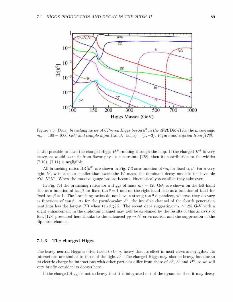
7.1. HIGGS PRODUCTION AND DECAY IN THE 2HDM–II 89
Figure 7.3: Decay branching ratios of CP-even Higgs boson h0 in the 4F2HDM-II for the mass-rangemh = 100 − 1000 GeV and sample input (tan β, tanα) = (1,−3). Figure and caption from [128].
is also possible to have the charged Higgs H± running through the loop. If the charged H± is veryheavy, as would seem fit from flavor physics constraints [128], then its contribution to the widths(7.10), (7.11) is negligible.
All branching ratios BR[h0]
are shown in Fig. 7.3 as a function of mh for fixed α, β. For a verylight h0, with a mass smaller than twice the W mass, the dominant decay mode is the invisibleν ′ν ′,N ′N ′. When the massive gauge bosons become kinematically accessible they take over.
In Fig. 7.4 the branching ratios for a Higgs of mass mh = 126 GeV are shown on the left-handside as a function of tan β for fixed tan θ = 1 and on the right-hand side as a function of tan θ forfixed tan β = 1. The branching ratios do not have a strong tan θ dependece, whereas they do varyas functions of tan β. As for the pseudoscalar A0, the invisible channel of the fourth generationneutrinos has the largest BR when tan β . 2. The recent data suggesting mh ≃ 125 GeV with aslight enhancement in the diphoton channel may well be explained by the results of this analysis ofRef. [128] presented here thanks to the enhanced gg → h0 cross section and the suppression of thediphoton channel.
7.1.3 The charged Higgs
The heavy neutral Higgs is often taken to be so heavy that its effect in most cases is negligible. Itsinteractions are similar to those of the light h0. The charged Higgs may also be heavy, but due toits electric charge its interactions with other particles differ from those of A0, h0 and H0, so we willvery briefly consider its decays here.
If the charged Higgs is not so heavy that it is integrated out of the dynamics then it may decay
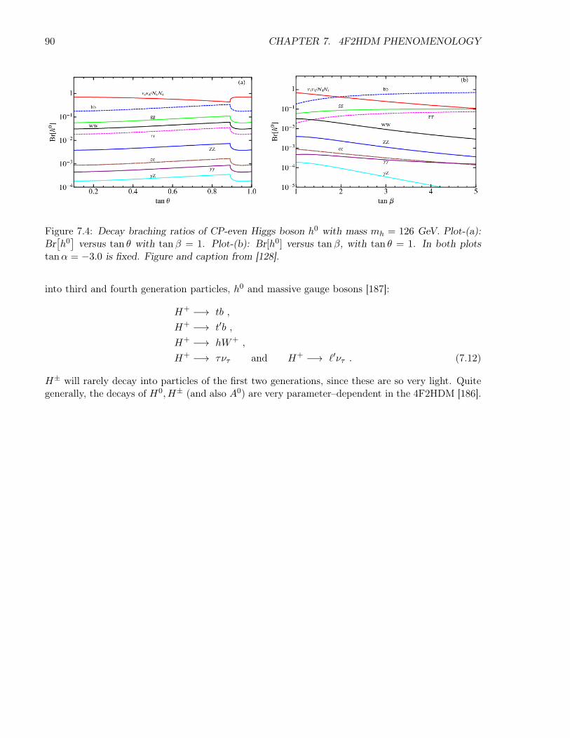
90 CHAPTER 7. 4F2HDM PHENOMENOLOGY
Figure 7.4: Decay braching ratios of CP-even Higgs boson h0 with mass mh = 126 GeV. Plot-(a):Br[h0]
versus tan θ with tan β = 1. Plot-(b): Br[h0] versus tan β, with tan θ = 1. In both plotstanα = −3.0 is fixed. Figure and caption from [128].
into third and fourth generation particles, h0 and massive gauge bosons [187]:
H+ −→ tb ,
H+ −→ t′b ,
H+ −→ hW+ ,
H+ −→ τντ and H+ −→ ℓ′ντ . (7.12)
H± will rarely decay into particles of the first two generations, since these are so very light. Quitegenerally, the decays of H0,H± (and also A0) are very parameter–dependent in the 4F2HDM [186].
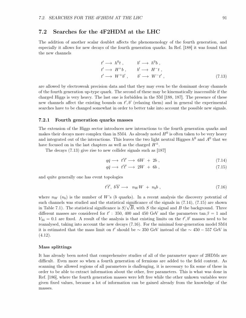
7.2. SEARCHES FOR THE 4F2HDM AT THE LHC 91
7.2 Searches for the 4F2HDM at the LHC
The addition of another scalar doublet affects the phenomenology of the fourth generation, andespecially it allows for new decays of the fourth generation quarks. In Ref. [188] it was found thatthe new channels
t′ −→ h0t , b′ −→ h0b ,
t′ −→ H+b , b′ −→ H−t ,
t′ −→ W+b′ , b′ −→ W−t′ , (7.13)
are allowed by electroweak precision data and that they may even be the dominant decay channelsof the fourth generation up-type quark. The second of these may be kinematically inaccessible if thecharged Higgs is very heavy. The last one is forbidden in the SM [188, 187]. The presence of thesenew channels affect the existing bounds on t′, b′ (relaxing them) and in general the experimentalsearches have to be changed somewhat in order to better take into account the possible new signals.
7.2.1 Fourth generation quarks masses
The extension of the Higgs sector introduces new interactions to the fourth generation quarks andmakes their decays more complex than in SM4. As already noted H0 is often taken to be very heavyand integrated out of the interactions. This leaves the two light neutral Higgses h0 and A0 that wehave focused on in the last chapters as well as the charged H±.
The decays (7.13) give rise to new collider signals such as [187]
qq −→ t′t′ −→ 6W + 2b , (7.14)
qq −→ t′t′ −→ 2W + 6b , (7.15)
and quite generally one has event topologies
t′t′, b′b′ −→ nWW + nbb , (7.16)
where nW (nb) is the number of W ’s (b quarks). In a recent analysis the discovery potential ofsuch channels was studied and the statistical significance of the signals in (7.14), (7.15) are shownin Table 7.1). The statistical significance is S/
√B, with S the signal and B the background. Three
different masses are considered for t′ : 350, 400 and 450 GeV and the parameters tan β = 1 andV34 = 0.1 are fixed. A result of the analysis is that existing limits on the t′, b′ masses need to bereanalysed, taking into account the new decays (7.16). For the minimal four-generation model SM4it is estimated that the mass limit on t′ should be ∼ 350 GeV instead of the ∼ 450 − 557 GeV in(4.12).
Mass splittings
It has already been noted that comprehensive studies of all of the parameter space of 2HDMs aredifficult. Even more so when a fourth generation of fermions are added to the field content. Asscanning the allowed regions of all parameters is challenging, it is necessary to fix some of these inorder to be able to extract information about the other, free parameters. This is what was done inRef. [186], where the fourth generation masses were left free while the other unkown variables weregiven fixed values, because a lot of information can be gained already from the knowledge of themasses.
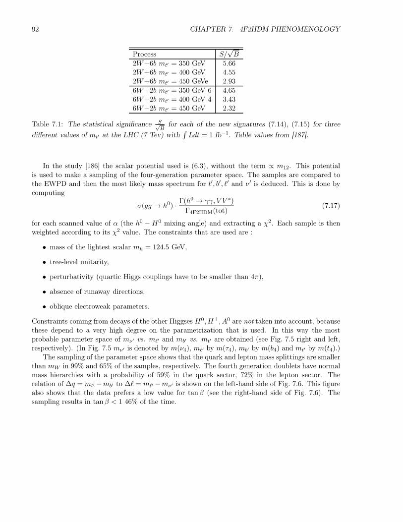
92 CHAPTER 7. 4F2HDM PHENOMENOLOGY
Process S/√B
2W+6b mt′ = 350 GeV 5.662W+6b mt′ = 400 GeV 4.552W+6b mt′ = 450 GeVe 2.93
6W+2b mt′ = 350 GeV 6 4.656W+2b mt′ = 400 GeV 4 3.436W+2b mt′ = 450 GeV 2.32
Table 7.1: The statistical significance S√B
for each of the new signatures (7.14), (7.15) for three
different values of mt′ at the LHC (7 Tev) with∫Ldt = 1 fb−1. Table values from [187].
In the study [186] the scalar potential used is (6.3), without the term ∝ m12. This potentialis used to make a sampling of the four-generation parameter space. The samples are compared tothe EWPD and then the most likely mass spectrum for t′, b′, ℓ′ and ν ′ is deduced. This is done bycomputing
σ(gg → h0) · Γ(h0 → γγ, V V ∗)
Γ4F2HDM(tot)(7.17)
for each scanned value of α (the h0 −H0 mixing angle) and extracting a χ2. Each sample is thenweighted according to its χ2 value. The constraints that are used are :
• mass of the lightest scalar mh = 124.5 GeV,
• tree-level unitarity,
• perturbativity (quartic Higgs couplings have to be smaller than 4π),
• absence of runaway directions,
• oblique electroweak parameters.
Constraints coming from decays of the other Higgses H0,H±, A0 are not taken into account, becausethese depend to a very high degree on the parametrization that is used. In this way the mostprobable parameter space of mν′ vs. mℓ′ and mb′ vs. mt′ are obtained (see Fig. 7.5 right and left,respectively). (In Fig. 7.5 mν′ is denoted by m(ν4), mℓ′ by m(τ4), mb′ by m(b4) and mt′ by m(t4).)
The sampling of the parameter space shows that the quark and lepton mass splittings are smallerthan mW in 99% and 65% of the samples, respectively. The fourth generation doublets have normalmass hierarchies with a probability of 59% in the quark sector, 72% in the lepton sector. Therelation of ∆q = mt′ −mb′ to ∆ℓ = mℓ′ −mν′ is shown on the left-hand side of Fig. 7.6. This figurealso shows that the data prefers a low value for tan β (see the right-hand side of Fig. 7.6). Thesampling results in tan β < 1 46% of the time.
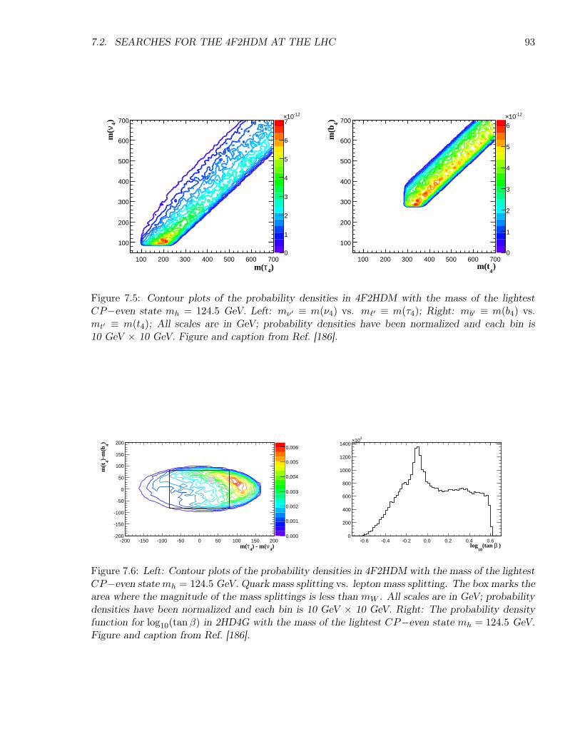
7.2. SEARCHES FOR THE 4F2HDM AT THE LHC 93
)4τm(100 200 300 400 500 600 700
) 4νm
(
100
200
300
400
500
600
700
0
1
2
3
4
5
6
7-1210×
)4
m(t100 200 300 400 500 600 700
) 4m
(b
100
200
300
400
500
600
700
0
1
2
3
4
5
6
-1210×
Figure 7.5: Contour plots of the probability densities in 4F2HDM with the mass of the lightestCP−even state mh = 124.5 GeV. Left: mν′ ≡ m(ν4) vs. mℓ′ ≡ m(τ4); Right: mb′ ≡ m(b4) vs.mt′ ≡ m(t4); All scales are in GeV; probability densities have been normalized and each bin is10 GeV × 10 GeV. Figure and caption from Ref. [186].
)4
ν) - m(4
τm(-200 -150 -100 -50 0 50 100 150 200
) 4)-
m(b
4m
(t
-200
-150
-100
-50
0
50
100
150
200
0.000
0.001
0.002
0.003
0.004
0.005
0.006
)β(tan 10
log-0.6 -0.4 -0.2 0.0 0.2 0.4 0.6
0
200
400
600
800
1000
1200
1400310×
Figure 7.6: Left: Contour plots of the probability densities in 4F2HDM with the mass of the lightestCP−even state mh = 124.5 GeV. Quark mass splitting vs. lepton mass splitting. The box marks thearea where the magnitude of the mass splittings is less than mW . All scales are in GeV; probabilitydensities have been normalized and each bin is 10 GeV × 10 GeV. Right: The probability densityfunction for log10(tan β) in 2HD4G with the mass of the lightest CP−even state mh = 124.5 GeV.Figure and caption from Ref. [186].

94 CHAPTER 7. 4F2HDM PHENOMENOLOGY
Chapter 8
Conclusions
In this thesis we have reviewed particle physics models with four generations of elementary particles.The motivation for studying such extensions of the standard model (SM) comes from the SM lackingexplanations for a number of phenomena observed in nature. Some of these issues are of fundamentalnature, such as the baryon asymmetry of the universe or the reason for family replication and thenumber of families. Other issues are of specific experimental nature: measurements whose resultscannot be accommodated in the SM (see Section 1.2.3 for details). An appealing feature of thefour-family models is that they agree with electroweak precision data and flavor observables. Forcertain observables, the agreement is even better in the four-generation scenario than it is in theSM.
Also, the nature of electroweak symmetry breaking and the origin of mass have been uncertainfor a long time, but at the moment the physics community is living exciting times, as a resonancehas just been observed (see Chapter 5). This resonance is presumably the much sought-after Higgsparticle. Its characteristics are not yet known, so whether it is standard model–like is not clear. Thefew pieces of information that lead to the discovery already suffice, however, to severely constrainmodels that incorporate new physics beyond the SM. Specifically, since the beginning of this work,the model which has been a major part of this work – the SM with four generations of elementaryparticles but just one scalar doublet (SM4) – has been excluded with a very high level of certainty (seeChapter 5). This is exciting in the sense that the SM4 is now the first of the popular new physics–models whose minimal version has been ruled out. (Some BSM models incorporate new physics atsuch scales that it is questionable whether they can be verified or excluded in the foreseeable future.)Just a few days before this thesis was submitted, the experimental exclusion of the SM4 was shownto have reached the very decisive statistical significance of 5.3σ (see Chapter 5 and Ref. [184]). Thisis possible thanks to the non-decoupling property of the fourth generation: the loop correctionsfrom the fourth generation do not tend towards zero when the masses of the particles are increased.
Pushing the extension further, following the exclusion of the minimal version, a perhaps ‘next-to-minimal’ model is one in which a scalar doublet is added to the SM along with the sequentialfourth family. This four-fermion two Higgs doublet model (4F2HDM), which is phenomenologicallyricher than the minimal one, can accommodate the new data from the LHC. The experimentalexclusion of the SM4 relies in part on the enhancement of Higgs production through gluon fusion inSM4 as opposed to the SM. In the two doublet model the light, neutral Higgses dominantly decayinto the fourth generation neutrinos in a large region of parameter space. (This decay, of course,requires that the neutrinos be kinematically accessible to the Higgs.)
Interestingly, these decays are invisible if the lifetime of the fourth generation neutrinos is largerthan the scale of the detector. The other, subdominant channels then get event rates that could
95
96 CHAPTER 8. CONCLUSIONS
match the observations. The partial decay widths depend on the parameters of the model, and inthe 4F2HDM notably upon the parameters tan β (giving the ratio of vacuum expectation values ofthe two scalar doublets) and tan θ (the neutrino mixing angle) and since the values of these are asyet unknown, no quantitative predictions can be made. Quite generally, given the number of freeparameters in the models with two Higgs doublets, it is difficult to perform comprehensive analysescovering the whole of the possible parameter space.
Precision measurements of the recently observed resonance – most likely the Higgs – are currentlybeing performed and more statistics will be accumulated in the near future. Hopefully, the newdata may soon give answers to some of the questions mentioned in this thesis.

Appendices
97

Appendix A
Definitions of electroweak observables
The following definitions are found for example in Ref. [189].
• The parameter χ2 is often used as a measure of the deviation from the central values of thetree level bounds of the global SM fit [111]
χ2
#(d.o.f.)≡ 1
n
∑
i=ud,us,ub,cd,cs,cb
( |VCKM4,i| − |Vi|∆Vi
)2
, (A.1)
where n is the number of considered degrees of freedom (d.o.f.).
• For the Z-pole measurements there are several observables that can be considered. Theone of interest to us is the observable sin 2β :
β = arg
(VcdV
∗cb
VtdV∗tb
), (A.2)
where Vij are the matrix elements of the CKM matrix.
• The front-back asymmetry AqqFB for a quark of flavor q is defined as
AqqFB =
σqF − σqBσqF + σqB
, (A.3)
where the cross-sections are integrated over the full forward (F) and backward (B) hemispheres,‘forward’ (‘backward’) meaning that the quark, rather than the antiquark, is produced atpositive (negative) cos θ.
• The left-right forward-backward asymmetry of a given event :
ALRFB =(σF − σB)L − (σF − σB)R(σF + σB)L + (σF + σB)R
× 1
〈|P|〉 , (A.4)
where the subscripts L,R define the helicities (left, right) of the initial-state particle and thebeam polarization P is taken as positive for right-handed beam helicity, negative for left and〈|P|〉 is the average of the absolute value of the polarization of the beam.
99
100 APPENDIX A. DEFINITIONS OF ELECTROWEAK OBSERVABLES
• The asymmetry parameter Af is defined for a fermion f and it is given by a relationbetween the couplings of left (L) and right (R) handed helicity states: gLf and gRf thecouplings of the left and right-handed ones, respectively, or equally well by a relation betweenthe axial (A) and vectorial (V) couplings gV f = gLf + gRf and gAf = gLf − gRf :
Af =g2Lf − g2Rf
g2Lf + g2Rf
=2gV fgAf
g2V f + g2Af
. (A.5)
• The average charge of all particles in a jet, called ‘jet charge’, gives information aboutthe charge of the original quark. The jet charge can be defined as
Qh =
∑i qip
κ||i∑
i pκ||i
, (A.6)
where the sum is over all charged particles in the hemisphere with charge qi and longitudinalmomentum with respect to the thrust axis p||i and κ is a parameter (usually fixed to have avalue between 0.3 and 1). Jet events are divided into two hemispheres by the plane perpen-dicular to the thrust axis. The jet charge in the forward (backward) hemisphere is denoted byQF (QB). Therefore QFB = QF −QB can be thought of as the forward-backward charge flow,which gives an effective observable, allowing for a derivation of the average charge asymmetry.
• The b-quark partial width of the Z-pole, normalized to the total hadronic width of theZ-peak, is
Rb =Γbb
Γhad, (A.7)
where Γbb is the width of the Z → bb decay and
Γhad =∑
q 6=t
Γqq (A.8)
is the hadronic width of the Z-pole (the top quark is excluded in the sum (A.8) because it iskinematically inaccessible: mt > mZ).
• The value for the effective leptonic mixing angle sin2 θℓeff, is derived from the experi-mental observables Af , given in Eq. (A.5) and
ALR =2(1 − 4 sin2 θfeff)
1 + (1− 4 sin2 θfeff)2
(A.9)
provided that the ratio of the vectorial to axial coupling of the given type of fermion is
gV f
gAf= 1− 2Qf
T f3
sin2 θfeff = 1− 4|Qf | sin2 θfeff . (A.10)
Appendix B
The Goldstone model
In this section we first review the Goldstone model, a field theory invariant under global U(1)transformations. This model necessarily leads to massless bosons – not photons – which are notobserved in nature, making them an undesirable and unphysical feature of the model. These bosonsare absent when spontaneous symmetry breaking is applied to a theory that is invariant under alocal symmetry transformation, i.e., to a gauge theory. In a gauge theory these so-called Nambu-Goldstone or Goldstone bosons have an interpretation as the longitudinal modes of the vector fields,making the vector fields behave as if they were massive. We will follow the presentations given inRefs. [190, 102, 191].
Non-invariance of the gound state
Consider a system whose Lagrangian density L possesses a particular symmetry, meaning that itis invariant under the corresponding group of symmetry transformations. When classifying theenergy levels of the system, there are two distinct cases: A given energy level can be non-degeneratemaking the corresponing energy eigenstate unique. In this case the eigenstate is invariant under thesymmetry goup of L. On the other hand the energy level might be degenerate and the correspondingenergy eigenstates are not invariant and transform linearly amongst themselves under the symmetrytransformations of L. A particular eigenstate is the state of lowest energy, the vacuum. A non-degenerate vacuum is unique and posesses the symmetries of L; on the other hand, when it isdegenerate there is no unique state to represent the vacuum. A vacuum may then be arbitrarilychosen and due to degeneracy it will not be invariant under the symmetries of L, it is asymmetric.This is called spontaneous symmetry breaking.
Non-invariance in the Hamiltonian formalism
Whenever an interaction posseses some symmetry a given problem is often simplified considerably.Exact symmetries (such as electric charge conservation) are fairly rare in nature, and one oftenassumes the system to be such that it is just a small piece of the Hamiltonian H or LagrangianL density that violates a particular symmetry whereas the rest of H or L is invariant. (This isthe case in the SM: strong interactions conserve parity, isospin and strangeness, but at the sametime electromagnetic interactions violate isospin and weak interactions violate isospin, parity andstrangeness, so a hierarchy of forces arise.)
Let a system be described by such a Hamiltonian that can be written in parts as
H = H0 + λH1 , (B.1)
101
102 APPENDIX B. THE GOLDSTONE MODEL
where H0 is invariant under some group of transformations wheras H1 is not and λ is a parameter.When there is an element U of the symmetry group that leaves the Hamiltonian H0 invariant, then
UH0U† = H0 , (B.2)
and U connects states that form an irreducible representation of the group
U |A〉 = |B〉 . (B.3)
It follows that the energies of states related in the way of (B.3) are equal :
EA = 〈A|H0|A〉 = 〈B|H0|B〉 = EB . (B.4)
This is just a statement of the degeneracy of the states |A〉 and |B〉, and so the symmetry of theHamiltonian is manifest in the degeneracy of the energy eigenstates that correspond to the irreduciblerepresentations of the symmetry group.
When the formalism of creation and annihilation operators is used, the states |A〉 and |B〉 canbe related to the ground state |0〉 through some creation operators φA and φB
|A〉 = φA|0〉 , |B〉 = φB |0〉 (B.5)
which satisfy
UφAU† = φB . (B.6)
Hence Eq. (B.3) is satisfied only if
U |0〉 = |0〉 . (B.7)
When Eq. (B.7) is not satisfied the equality in Eq. (B.3) is violated and the symmetry consequenceof the degenerate energy levels no longer hols. This situation is often referred to as a sponta-neous symmetry breakdown. The Hamiltonian (or Lagrangian) is still invariant under the symmetrytransformation even though the symmetry is no longer manifest in the degenerate energy levels.
Goldstone’s theorem
Let us consider the Lagrangian density of a complex scalar field φ(x) :
L = (∂µφ∗)(∂µφ)− µ2φφ∗ − λ(φφ∗)2 , (B.8)
called the Goldstone Lagrangian density. This density is invariant under the U(1) group of globaltransformations
φ(x) −→ φ′(x) = e−iαφ(x) , (B.9)
with α an arbitrary parameter that does not depend on the spacetime coordinates x. The kineticterm in (B.8) is positive and vanishes only if φ(x) is constant. The ground state of the system isobtained at the minimum of the ‘potential’
V (φ) ≡ µ2φφ∗ + λ(φφ∗)2 . (B.10)
As V (φ) depends on φ and φ∗ only through φφ∗ = |φ|2 we can ease the notation by defining
ρ ≡ φφ∗ , (B.11)

103
so that (B.10) becomes a functional of ρ
V (φ) → V (ρ) = µ2ρ+ λρ2 . (B.12)
The potential has a minimum only if λ > 0, which we therefore take to be true. Interpreting µ2 asa conventional mass term > 0, the potential has a symmetric ground state at φ = 0. This groundstate is unique and symmetric under (B.9). On the other hand, if µ2 < 0 the minimum is at
ρ = −µ2
2λ, (B.13)
which implies that there exists a whole ring of radius |φ| = √ρ in the complex φ plane whose points
give the minumum of the potential V . Defining
v ≡√
−µ2λ
, (B.14)
the ring of minima is at
|φ| = v√2. (B.15)
The point φ = 0 is now unstable, whereas the number of stable points satisfying Eq. (B.15) isinfinite. Each of the points in the ground state can be reached from another ground state point bya U(1) transformation. For a point on the real axis
φ(x) =1√2[v + ξ(x) + iχ(x)] , (B.16)
with ξ, χ ∈ ℜ and ξ = χ = 0 in the ground state. Substituting this into the Godstone Lagrangian(B.8) and ignoring constant terms gives
L =1
2(∂µξ)
2 +1
2(∂µχ)
2 − λv2ξ2 − λvξ(ξ2 + χ2)− 1
4λ(ξ2 + χ2)2 . (B.17)
Interpreting the Lagrangian (B.17) as one describing a quantum field theory with two basic fields ξand χ, we see that there is no mass term for the field χ, but that there is a mass term of the usualform −1
2m2ξξ
2 for ξ with
m2ξ = 2λv2 . (B.18)
What has happened is that starting with an L, constructed from a complex scalar field φ(x),invariant under U(1) and with µ2 < 0 we have ended with two fields: a massless field χ and a fieldξ whose mass (B.18) has been generated ‘spontaneously’.
When the Lagrangian (B.8) is generalized from one to n real scalar fields φj :
L =∑
j
1
2(∂µφj)(∂
µφj)−1
2µ2φjφj − λ(φjφj)
2
(B.19)
its symmetry group is the n-dimensional orthogonal group O(n) with 12n(n − 1) generators. The
symmetry group mixes the fields with each other. The gound state is again the ‘ring’ at∑
j φjφj =
−µ2/4λ when µ2 < 0. Thinking of the fields φj as components of a vector Φ, then the ground statefixes the length of this vector but leaves its direction arbitrary. Therefore one is free to choose justone of the components of Φ to be nonzero, say the nth one. All other vacua can then be obtainedfrom this chosen one by an O(n) transformation. (Physically, the various equivalent ground states
104 APPENDIX B. THE GOLDSTONE MODEL
differ according to the number of Goldstone bosons (of zero energy and momentum) that theycontain.) The difference to the previously considered case is that the chosen a vacuum state
Φvac =
00...0v
(B.20)
is now invariant under a nontrivial subgroup of O(n), namely under O(n − 1), that mixes then − 1 first components amongst themselves but does not touch the nth component. The groupO(n− 1) has 1
2 (n− 1)(n− 2) generators. Thus the difference in the number of geenrators betweenthe original group O(n) and the residual group O(n − 1) equals n − 1. These correspond to then− 1 ‘broken generators’ of the original symmetry group, playing the role of the Goldstone bosonsor the longitudinal polarizations of vector bosons.
Repeating the calculation of Eqs. (B.16)–(B.18) one sees that there is still just one massivefield and that the n − 1 other fields, called ‘Goldstones’, remain massless. The above consideredcases are examples of the Goldstone theorem [192] (also [193, 60, 61]) viable for any symmetry group:
For every broken generator in a spontaneous symmetry breakingthere exists a massless scalar boson.
Appendix C
Mathematical description of neutrino
oscillations
Neutrino flavor change is the process να → νβ, such that α 6= β, i. e. a neutrino with flavor αbecomes one with a different flavor, β. This quantum mechanical phenomenon happens both forneutrinos propagating in vacuum and in matter. In most experiments neutrinos are produced bycharged current weak interactions. A neutrino beam is a superposition of various particle eigen-states, which evolve differently as the beam propagates and the probability of finding differenteigenstates in the beam varies with time. This phenomenon, which is a consequence of neutrinomixing, is called neutrino oscillation.
Let us consider charged current interactions, resulting in charged antileptons ℓ and neutrinos νℓ.The neutrinos participating in weak interactions are in the interaction basis, which is different fromthe mass eigenstates [194]. A physically observable state in the interaction basis is generally asuperposition of the matter states να with masses mα :
|νℓ〉 =∑
α
Uℓα|να〉 , (C.1)
where U ∈ U(N) is the amplitude of the process (see also Section 2.5.2). Let us for simplicityassume that all neutrinos in the beam have the same three–momentum p. Since the masses of thecomponents differ the energies of the various components cannot be equal, as follows from
E2α = p2 +m2
α , pα = p ∀ α . (C.2)
The evolution of states is given by standard quantum mechanics (see e.g. [195]), so that at a timet the beam has evolved from the initial state at t = 0 to
|νℓ(t)〉 =∑
α
e−iHαtUℓα|να〉 =∑
α
e−iEαtUℓα|να〉 , (C.3)
with |να〉 ≡ |να(t = 0)〉. This result (C.3) holds under the assumption that neutrinos are stableparticles.
As already noted in (C.2), the different Eα’s are not equal. The superposition (C.3) is differentfrom (C.1). The amplitude of a state νℓ′ in the state |νℓ(t)〉 is
〈νℓ′ |νℓ(t)〉 =∑
α,β
〈νβ|U †βℓ′e
−iEαtUℓα|να〉 (C.4)
105

106 APPENDIX C. MATHEMATICAL DESCRIPTION OF NEUTRINO OSCILLATIONS
and the probability of finding the state νℓ′ is
Pνℓνℓ′ (t) = |〈νℓ′ |νℓ(t)〉|2
=∑
α,β
|UℓαU∗ℓ′αU
∗ℓβUℓ′β| cos
[(Eα − Eβ)t− ϕℓℓ′αβ
], (C.5)
where we have used the fact that the mass eigenstates are orthonormal, 〈νℓ′ |νℓ〉 = δℓ′ℓ and ϕℓℓ′αβ isdefined as
ϕℓℓ′αβ = arg(UℓαU∗ℓ′αU
∗ℓβUℓ′β) . (C.6)
Neutrinos are usually ultrarelativistic, so
Eα ≃ |p|+ m2α
2|p| . (C.7)
In the ultrarelativistic limit t may be replaced by the distance traveled at that time, say x (sincev ≃ c = 1), giving the probability (C.5)
Pνℓνℓ′ (t) =∑
α,β
|UℓαU∗ℓ′αU
∗ℓβUℓ′β| cos
(2πx
Lαβ− ϕℓℓ′αβ
), (C.8)
with
Lαβ ≡ 4π|p|∆m2
αβ
(C.9)
and∆m2
αβ ≡ m2α −m2
β . (C.10)
The oscillation lengths |Lαβ | give a distance scale over which the effects of oscillation are discernible.For all distances x 6= n · Lαβ , n ∈ Z, the effects of oscillation are nontrivial.
Experimental values
In order to cite values given in the literature [55] for the above parameters we need to specify theotherwise completely arbitrary numbering of the neutrinos, νi. We choose to identify |∆m2
21| withthe smaller of the neutrino mass differences squared and for convenience that m1 < m2 so that∆m2
21 > 0. Which other mass difference is chosen as the second independent parameter does notreally matter, since in fact |∆m2
21| ≪ |∆m231(32)|, |∆m2
21|/|∆m231(32)| ≈ 0.03 and ∆m2
31 ≃ ∆m232 (for
motivation, see Ref. [55]). The current values of the parameters are shown in Table C.1, where theupper (lower) row corresponds to normal (inverted) neutrino mass hierarchy, where ‘normal’ and‘inverted’ mass hierarchies correspond to |∆m2
31| > |∆m232| and |∆m2
32| > |∆m231|, respectively.
Parameter Best fit ±1σ
∆m221
[10−5eV2
]7.59+0.20
−0.18
∆m231
[10−3eV2
] 2.4 ± 0.09
−(2.34+0.10
−0.09
)
Table C.1: Values of neutrino mixing parameters ∆m2αβ. For ∆m2
31 the upper (lower) row corre-sponds to normal (inverted) neutrino mass hierarchy. Values from Ref. [129]
Appendix D
Oblique electroweak parameters
While the SU(2)×U(1)Y gauge theory of electroweak interactions is widely accepted the mechanismresponsible for the breaking SU(2)L × U(1)Y → U(1)Q, called the Higgs sector, is still a mystery.There is a multitude of alternative models (several Higgs doublets, technicolor etc.), but none ofthe particles predicted by these models have yet been discovered directly 1, so it is important tomake use of indirect information from current measurements. The most important constraints comefrom the measurement of weak interaction parameters, which are typically measured at a very highprecision: typically to a part per mil [196].
The most general Higgs models allow for large deviations from the SM predictions. In the 70’s itwas noted that in the SM there is a ‘natural’ tree–level quantity called the ρ–parameter (2.62) thatcan be used to restrict models that break the electroweak symmetry. The theoretically predictedvalue for the ρ–parameter is unity (2.63) in the SM, a value that is in agreement with experiment(the deviation is smaller than 1%), so it is reasonable to assume that the corrections to this relationarise from radiative corrections only [137]. The radiative corrections are sensitive to new particlesgoing through the loops.
Later it was noted that the effects of vacuum–polarization diagrams, as in Fig. D.1, so–calledoblique corrections, could also be used as a tool to scrutinize new–physics models in a generalway [197] and this idea was incorporated into a complete theory of weak radiative corrections [198,199, 200].
In many studies about the fourth generation these oblique corrections are used to constrainthe parameter space of the SM4. A possible fourth generation affects many amplitudes throughloop diagrams, and for the Z and W bosons the effects of new heavy quarks and leptons enteronly through vacuum–polarization diagrams. In this section we will consider the physics of thesediagrams in some detail, following the presentation given in Ref. [137]
Vacuum polarizations affect the gauge interactions indirectly by modifying the gaugeboson propagators. This is why they are called ‘oblique’ corrections as opposed to ‘direct’ vertexand box corrections, which directly affect the form of the interaction. The vacuum polarizationamplitudes are defined as ΠXY (q
2), with (XY ) = (11), (22), (33), (3Q) and (QQ), by
igµνΠXY (q2) + (qµqν terms) ≡
∫d4x e−iqx〈Jµ
X(x)JνY (0)〉 . (D.1)
1At the time of finishing this report, in July 2012, a resonance has been seen at ∼ 125 GeV by the ATLAS [100]and CMS [101] collaborations at the LHC and also by D0 and CDF at the Tevatron [180]. The observed decays hintat this being the Higgs boson.
107
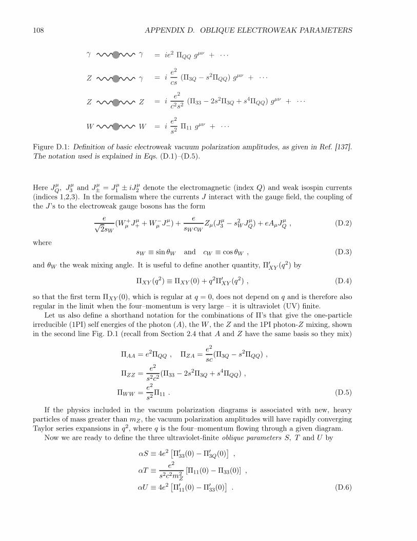
108 APPENDIX D. OBLIQUE ELECTROWEAK PARAMETERS
γ γ
Z γ
Z Z
W W
= ie2 ΠQQ gµν + · · ·
= ie2
cs(Π3Q − s2ΠQQ) g
µν + · · ·
= ie2
c2s2(Π33 − 2s2Π3Q + s4ΠQQ) g
µν + · · ·
= ie2
s2Π11 g
µν + · · ·
Figure D.1: Definition of basic electroweak vacuum polarization amplitudes, as given in Ref. [137].The notation used is explained in Eqs. (D.1)–(D.5).
Here JµQ, J
µ3 and Jµ
± = Jµ1 ± iJµ
2 denote the electromagnetic (index Q) and weak isospin currents(indices 1,2,3). In the formalism where the currents J interact with the gauge field, the coupling ofthe J ’s to the electroweak gauge bosons has the form
e√2sW
(W+µ J
µ+ +W−
µ Jµ−) +
e
sW cWZµ(J
µ3 − s2WJ
µQ) + eAµJ
µQ , (D.2)
wheresW ≡ sin θW and cW ≡ cos θW , (D.3)
and θW the weak mixing angle. It is useful to define another quantity, Π′XY (q
2) by
ΠXY (q2) ≡ ΠXY (0) + q2Π′
XY (q2) , (D.4)
so that the first term ΠXY (0), which is regular at q = 0, does not depend on q and is therefore alsoregular in the limit when the four–momentum is very large – it is ultraviolet (UV) finite.
Let us also define a shorthand notation for the combinations of Π’s that give the one-particleirreducible (1PI) self energies of the photon (A), the W , the Z and the 1PI photon-Z mixing, shownin the second line Fig. D.1 (recall from Section 2.4 that A and Z have the same basis so they mix)
ΠAA = e2ΠQQ , ΠZA =e2
sc(Π3Q − s2ΠQQ) ,
ΠZZ =e2
s2c2(Π33 − 2s2Π3Q + s4ΠQQ) ,
ΠWW =e2
s2Π11 . (D.5)
If the physics included in the vacuum polarization diagrams is associated with new, heavyparticles of mass greater than mZ , the vacuum polarization amplitudes will have rapidly convergingTaylor series expansions in q2, where q is the four–momentum flowing through a given diagram.
Now we are ready to define the three ultraviolet-finite oblique parameters S, T and U by
αS ≡ 4e2[Π′
33(0) −Π′3Q(0)
],
αT ≡ e2
s2c2m2Z
[Π11(0)−Π33(0)] ,
αU ≡ 4e2[Π′
11(0) −Π′33(0)
]. (D.6)

109
Several different notations for these parameters appear in the literature. The above parameters arewritten in terms of e, θW and mZ since these are some of the most accurately measured parametersof electroweak interactions and serve as good reference points. Of the three listed in (D.6), theS and T parameters divide the contribution of electroweak radiative corrections into pieces whichhave a distinct physical significance:
S is isospin-symmetric and gives a part of the momentum dependence of Π33, the part that isultraviolet finite,
T obtains contributions only from effects that violate a global SU(2) symmetry called a custodialsymmetry.
In fact S can be pictured as measuring the total size of the new sector while T measures the totalisospin-breaking induced by this new sector. U is often predicted to be very small.
Provided that the mass scale of new physics is high and that the main contribution from itmostly comes from virtual loops to the electroweak observables, then the three oblique parametersprovide a representation of the discrepancies expected from nonstandard physics. All neutral-currentand low-energy observables depend only on S and T , whereas the only accurately measured weakinteraction observable that depends on U is mW .
The use of S,T,U is convenient as it allows for the predictions from various models to becompared with electroweak precision data. For a given model, the prediction of any electroweakobservable O is [172]
O = OSM,ref(MH,ref,mt,ref) + cSS + cTT + cUU , (D.7)
where OSM,ref is the SM prediction of the observable in the SM and cS , cT , cU are constants. TheSM reference depends on MH and mt, which take fixed values, and includes all known higher–orderelectroweak corrections. The parameters cS , cT , cU can be found in the literature [55] for the fullset of electroweak observables. Because these have been measured with such high precision, theoblique parameters of various BSM models are restricted by the relation (D.7).
As can be seen from (D.7), S, T and U all vanish in the SM. As our interest in this report is inthe physics of SM4 we note that each extra fermion doublet that is put into the theory contributesadditively to both S and T , because the contribution from a fermion doublet (u, d) is [137]
S(xu, xd) =Nc
6π
[1− Y log
(xuxd
)], (D.8)
T (xu, xd) =Nc
16πs2W (1− s2W )
[xu + xd −
2xuxdxu − xd
log
(xuxd
)], (D.9)
U(xu, xd) =Nc
6π
[−5x2u − 22xuxd + 5x2d
3(xu − xd)2+x3u − 3x2uxd − 3xuxd + x2d
(xu − xd)3log
(xuxd
)], (D.10)
where xf ≡ m2f/m
2Z , Nc is the number of colors (Nc=3 for quarks and Nc=1 for leptons) and Y
is the hypercharge of the doublet. The total contribution to the S, T, U parameters from a fourthgeneration is obtained when both quark and lepton doublets are taken into account in the relations(D.8)–(D.10) and the mixing with the third family (which is assumed dominant – mixings to the
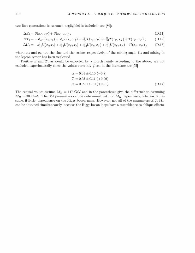
110 APPENDIX D. OBLIQUE ELECTROWEAK PARAMETERS
two first generations is assumed negligible) is included, too [86]:
∆S4 = S(xt′ , xb′) + S(xℓ′ , xν′) , (D.11)
∆T4 = −s234T (xt, xb) + s234T (xt′ , xb) + s234T (xt, xb′) + c234T (xt′ , xb′) + T (xℓ′ , xν′) , (D.12)
∆U4 = −s234U(xt, xb) + s234U(xt′ , xb) + s234U(xt, xb′) + c234U(xt′ , xb′) + U(xℓ′ , xν′) , (D.13)
where s34 and c34 are the sine and the cosine, respectively, of the mixing angle θ34 and mixing inthe lepton sector has been neglected.
Positive S and T , as would be expected by a fourth family according to the above, are notexcluded experimentally since the values currently given in the literature are [55]
S = 0.01± 0.10 (−0.8)
T = 0.03± 0.11 (+0.09)
U = 0.09± 0.10 (+0.01) (D.14)
The central values assume MH = 117 GeV and in the parenthesis give the difference to assumingMH = 300 GeV. The SM parameters can be determined with no MH dependence, whereas U hassome, if little, dependence on the Higgs boson mass. However, not all of the parameters S, T,MH
can be obtained simultaneously, because the Higgs boson loops have a resemblance to oblique effects.
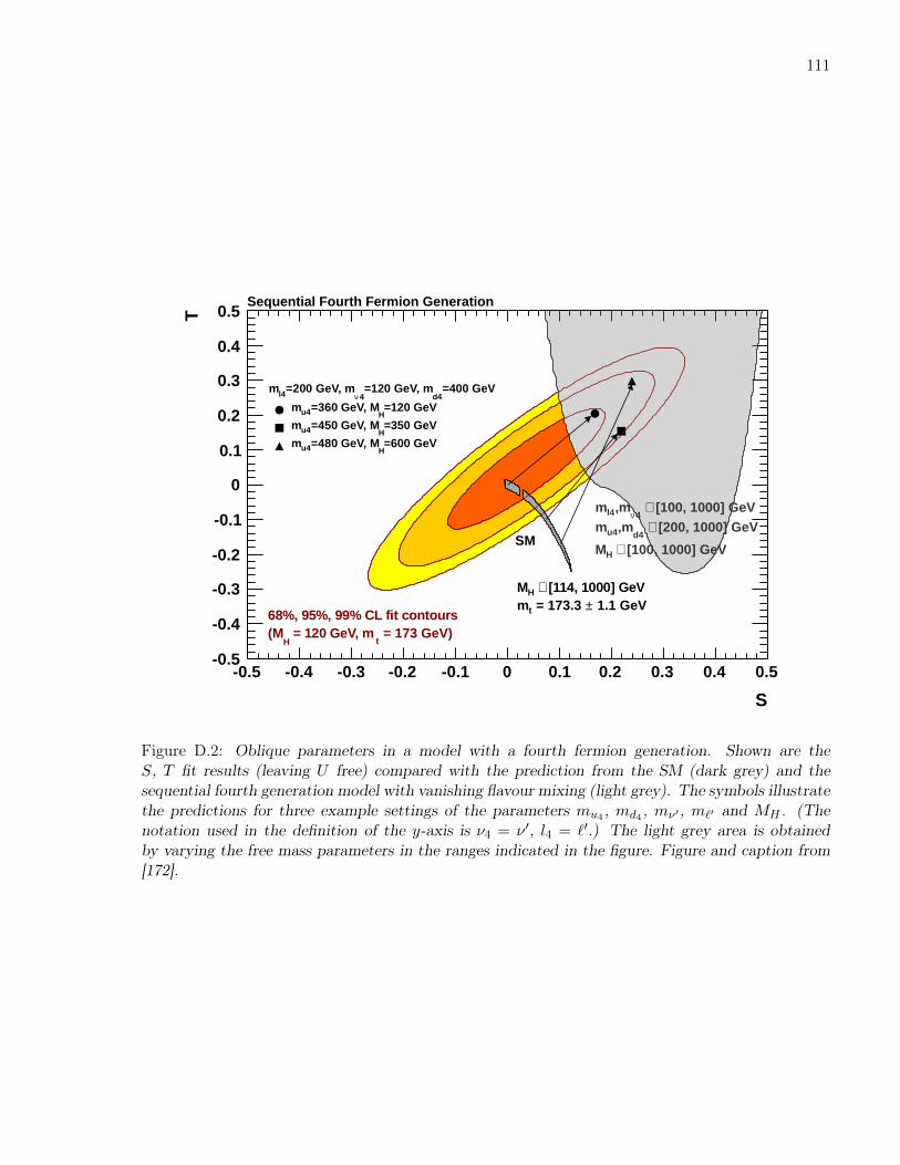
111
S
-0.5 -0.4 -0.3 -0.2 -0.1 0 0.1 0.2 0.3 0.4 0.5
T
-0.5
-0.4
-0.3
-0.2
-0.1
0
0.1
0.2
0.3
0.4
0.5
SM
[114, 1000] GeV∈ HM 1.1 GeV± = 173.3 tm
[100, 1000] GeV∈ 4ν
,ml4m [200, 1000] GeV∈
d4,mu4m
[100, 1000] GeV∈ HM
=400 GeVd4
=120 GeV, m4ν
=200 GeV, ml4m
=120 GeVH
=360 GeV, Mu4m
=350 GeVH
=450 GeV, Mu4m
=600 GeVH
=480 GeV, Mu4m
Sequential Fourth Fermion Generation
68%, 95%, 99% CL fit contours = 173 GeV)
t = 120 GeV, m
H(M
Figure D.2: Oblique parameters in a model with a fourth fermion generation. Shown are theS, T fit results (leaving U free) compared with the prediction from the SM (dark grey) and thesequential fourth generation model with vanishing flavour mixing (light grey). The symbols illustratethe predictions for three example settings of the parameters mu4
, md4 , mν′ , mℓ′ and MH . (Thenotation used in the definition of the y-axis is ν4 = ν ′, l4 = ℓ′.) The light grey area is obtainedby varying the free mass parameters in the ranges indicated in the figure. Figure and caption from[172].
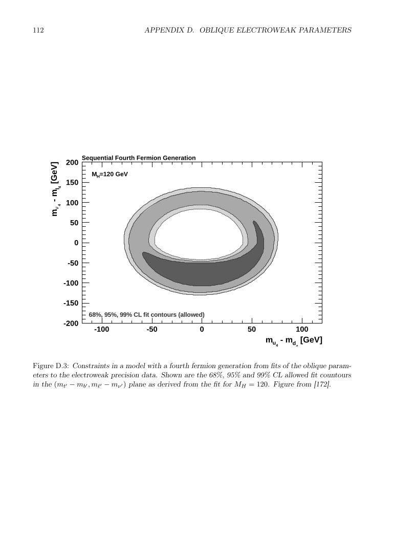
112 APPENDIX D. OBLIQUE ELECTROWEAK PARAMETERS
[GeV]4
d - m4um
-100 -50 0 50 100
[GeV
]4l
- m
4νm
-200
-150
-100
-50
0
50
100
150
200Sequential Fourth Fermion Generation
68%, 95%, 99% CL fit contours (allowed)
=120 GeVHM
Figure D.3: Constraints in a model with a fourth fermion generation from fits of the oblique param-eters to the electroweak precision data. Shown are the 68%, 95% and 99% CL allowed fit countoursin the (mt′ −mb′ ,mℓ′ −mν′) plane as derived from the fit for MH = 120. Figure from [172].

Appendix E
Feynman diagrams for production of
fourth family particles
t′, b′
t′, b′
(a)
q
g
W
q′
t′, b′
t′, b′(b)
q
g
W
q′
t′, b′
b, t(c)
Figure E.1: Production of fourth generation quarks. (a) Strong pair production of heavy quarks atleading order, (b) 2 → 3 Born diagrams contributing to t′b′ and t′b′ and (c) t′b and tb′ t–channelelectroweak production. The amplitude of (c) us suppressed if the 3–4 CKM mixing is small.Diagrams as in [154].
e+
qW+
νe
t′ b
(a)W+
e−
qW−
t′
νe
b
W−(b)
Figure E.2: The diagrams for single production of fourth family t′ (a) and t′ (b) quarks in epcollisions, as given in Ref. [152].
113

114APPENDIX E. FEYNMAN DIAGRAMS FOR PRODUCTION OF FOURTH FAMILY PARTICLES
e−
qW+
νe
b′ c
(a)W−
e+
qW+
b′
νe
c
W+
(b)
Figure E.3: The diagrams for single production of fourth family b′ (a) and b′ (b) quarks in epcollisions, as given in Ref. [156].
q
qW+
Q′
q′
q
q′W+
Q′
q′′
q
q
W+ Q′
q′′
(a) (b) (c)
Figure E.4: The diagrams for single production of fourth family quarks Q in pp collisions. Diagramsas in Ref. [153].
qi
g
qiqj
W±
(a)
qi
g
qj
W±
qj
(b)
qi
g
t′
W±
qj
(c)
qi
g
t′qj
W±
(d)
Figure E.5: The diagrams for gqi → W+qj subprocesses including t′qg anomalous vertices. qi is aquark from the proton and qj is a quark of any flavor depending on the charged current interaction.For W−qj final states one may change the direction of the current lines and replace the outgoingquarks with incoming antiquarks. Diagrams and caption from Ref. [158].
q
q
Z ν ′
ν ′
g
g
qh
ν ′
ν ′
Figure E.6: The ν ′ pair production of via netral current (left) and Higgs interaction (right). Dia-grams as in Ref. [148].

115
g
g
qh
Z
Z
ℓ
ℓ
ℓ
ℓg
g
qh
ν ′
ν ′ℓ
W
W
ℓ
Figure E.7: The ‘golden’ (left) and ‘silver’ (right) modes for the discovery of a heavy Higgs boson.For the golden mode ℓ = e, µ while for the silver mode ℓ = µ only. Diagrams as in Ref. [167].

116APPENDIX E. FEYNMAN DIAGRAMS FOR PRODUCTION OF FOURTH FAMILY PARTICLES
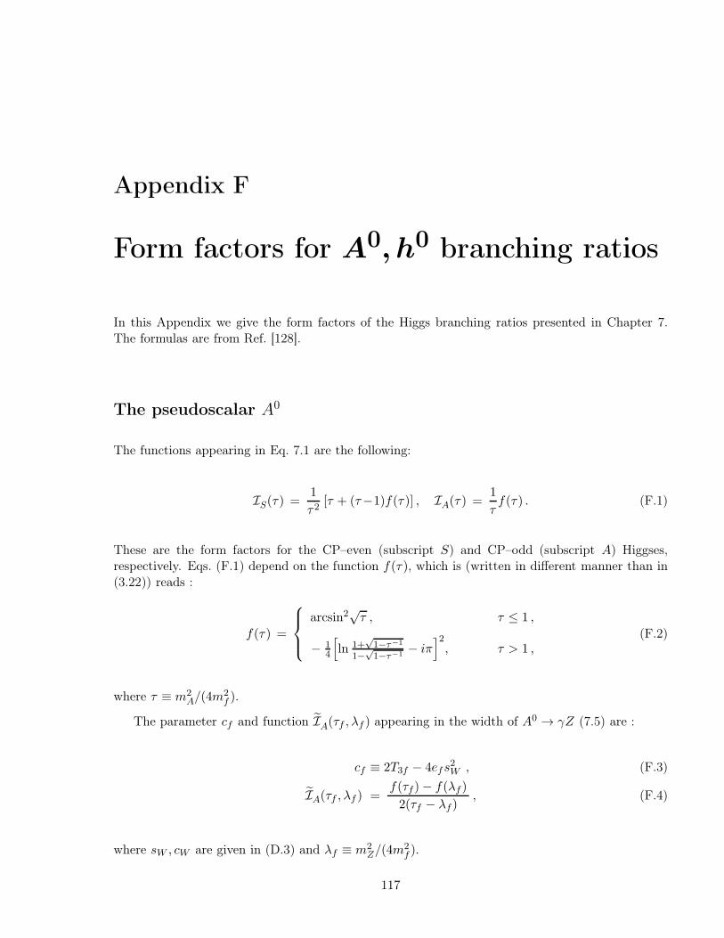
Appendix F
Form factors for A0, h0 branching ratios
In this Appendix we give the form factors of the Higgs branching ratios presented in Chapter 7.The formulas are from Ref. [128].
The pseudoscalar A0
The functions appearing in Eq. 7.1 are the following:
IS(τ) =1
τ2[τ + (τ−1)f(τ)] , IA(τ) =
1
τf(τ) . (F.1)
These are the form factors for the CP–even (subscript S) and CP–odd (subscript A) Higgses,respectively. Eqs. (F.1) depend on the function f(τ), which is (written in different manner than in(3.22)) reads :
f(τ) =
arcsin2√τ , τ ≤ 1 ,
− 14
[ln 1+
√1−τ−1
1−√1−τ−1
− iπ]2, τ > 1 ,
(F.2)
where τ ≡ m2A/(4m
2f ).
The parameter cf and function IA(τf , λf ) appearing in the width of A0 → γZ (7.5) are :
cf ≡ 2T3f − 4efs2W , (F.3)
IA(τf , λf ) =f(τf)− f(λf )
2(τf − λf ), (F.4)
where sW , cW are given in (D.3) and λf ≡ m2Z/(4m
2f ).
117
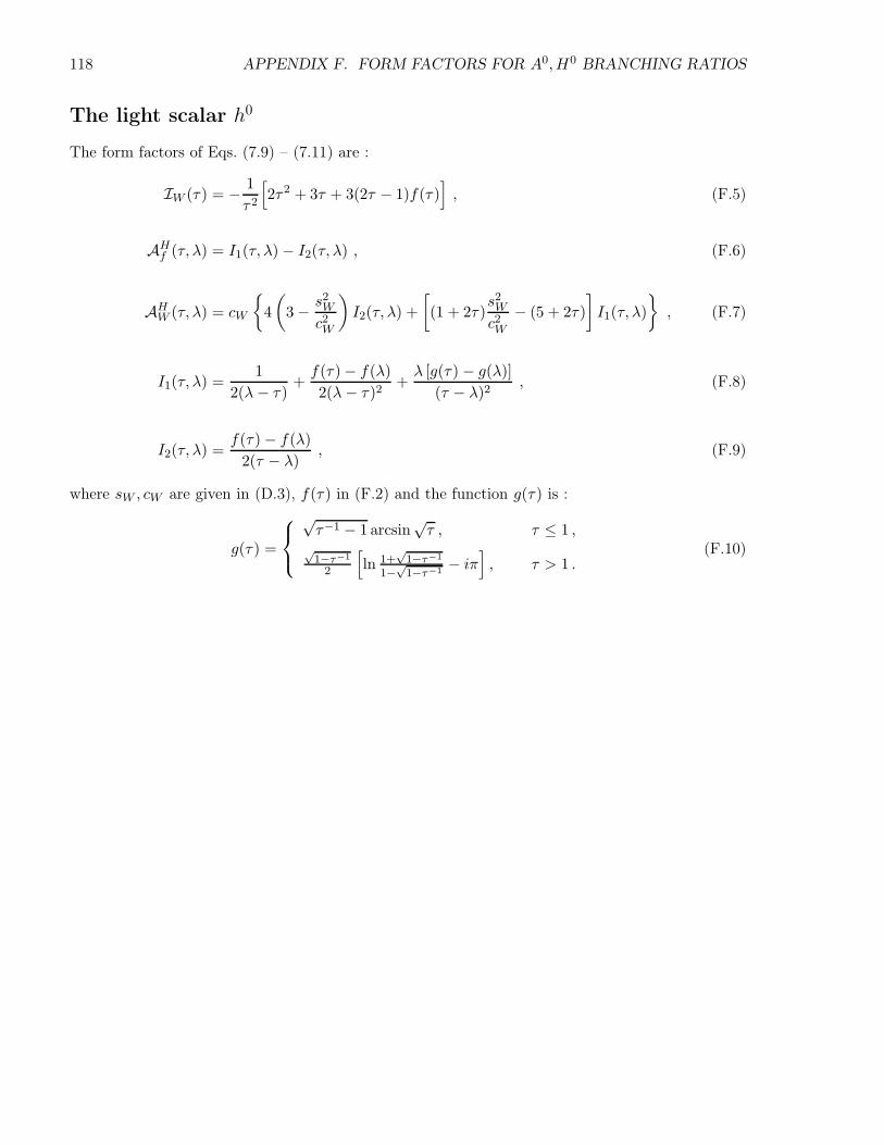
118 APPENDIX F. FORM FACTORS FOR A0,H0 BRANCHING RATIOS
The light scalar h0
The form factors of Eqs. (7.9) – (7.11) are :
IW (τ) = − 1
τ2
[2τ2 + 3τ + 3(2τ − 1)f(τ)
], (F.5)
AHf (τ, λ) = I1(τ, λ)− I2(τ, λ) , (F.6)
AHW (τ, λ) = cW
4
(3− s2W
c2W
)I2(τ, λ) +
[(1 + 2τ)
s2Wc2W
− (5 + 2τ)
]I1(τ, λ)
, (F.7)
I1(τ, λ) =1
2(λ− τ)+f(τ)− f(λ)
2(λ− τ)2+λ [g(τ) − g(λ)]
(τ − λ)2, (F.8)
I2(τ, λ) =f(τ)− f(λ)
2(τ − λ), (F.9)
where sW , cW are given in (D.3), f(τ) in (F.2) and the function g(τ) is :
g(τ) =
√τ−1 − 1 arcsin
√τ , τ ≤ 1 ,
√1−τ−1
2
[ln 1+
√1−τ−1
1−√1−τ−1
− iπ], τ > 1 .
(F.10)

Bibliography
[1] Hideki Yukawa. On the interaction of elementary particles. Proc. Phys. Math. Soc. Jap., 17:48–57,1935.
[2] W. Pauli. Letter to Lise Meitner on December 4. For a copy of the letter, see the Pauli letters collection:http://cdsweb.cern.ch/record/83282/files/ , 1930.
[3] Seth H. Neddermeyer and Carl D. Anderson. Note on the nature of cosmic-ray particles. Phys. Rev.,51(10):884–886, May 1937.
[4] J. C. Street and E. C. Stevenson. New evidence for the existence of a particle of mass intermediatebetween the proton and electron. Phys. Rev., 52(9):1003–1004, Nov 1937.
[5] Rabi, I. I. 1937. Cited in e.g. Cahn, R. N. and Goldhaber, G. The Experimental Foundations of Particle
Physics. Cambridge University Press, 1989.
[6] C. M. G. Lattes, H. Muirhead, G. P. S. Occhialini, and C. F. Powell. Processes involving chargedmesons. Nature, 159:694–697, 1947.
[7] C. M. G. Lattes, G. P. S. Occhialini, and C. F. Powell. Observations on the tracks of slow mesons inphotographic emulsions. 1. Nature, 160:453–456, 1947.
[8] C. M. G. Lattes, G. P. S. Occhialini, and C. F. Powell. Observations on the tracks of slow mesons inphotographic emulsions. 2. Nature, 160:486–492, 1947.
[9] G. D. Rochester and C. C. Butler. Evidence for the existence of new unstable elementary particles.Nature, 160:855–857, December 1947.
[10] J. Steinberger, W. K. H. Panofsky, and J. Steller. Evidence for the production of neutral mesons byphotons. Phys. Rev., 78:802–805, 1950.
[11] Jagdish Mehra and Helmut Rechenberg. The historical development of quantum theory. SpringerVerlag New York, Inc., 2001.
[12] L. Leprince-Ringuet and M. L’héritier. Existence probable d’une particule de masse 990 m0 dans lerayonnement cosmique. Comptes Rendus Acad. Sciences de Paris, page 618, séance du 13 Dec 1944.
[13] R. Brown, U. Camerini, P.H. Fowler, H. Muirhead, and D. M. Ritson. Observations with electron-sensitive plates exposed to cosmic radiation. Nature, 163:82–87, January 1949.
[14] T. Nakano and K. Nishijima. Charge Independence for V -particles. Prog. Theor. Phys., 10:581–582,1953.
[15] M. Gell-Mann. Isotopic Spin and New Unstable Particles. Phys. Rev., 92:833–834, 1953.
[16] Murray Gell-Mann. A Schematic Model of Baryons and Mesons. Phys. Lett., 8:214–215, 1964.
[17] George Zweig. CERN report 8182 / Th.401. Unpublished, 1964.
[18] O. W. Greenberg. Spin and Unitary Spin Independence in a Paraquark Model of Baryons and Mesons.Phys. Rev. Lett., 13:598–602, 1964.
[19] M. Y. Han and Yoichiro Nambu. Three-triplet model with double SU(3) symmetry. Phys. Rev.,139:B1006–B1010, 1965.
119
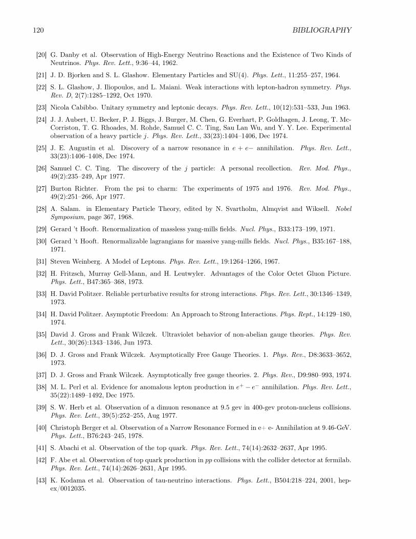
120 BIBLIOGRAPHY
[20] G. Danby et al. Observation of High-Energy Neutrino Reactions and the Existence of Two Kinds ofNeutrinos. Phys. Rev. Lett., 9:36–44, 1962.
[21] J. D. Bjorken and S. L. Glashow. Elementary Particles and SU(4). Phys. Lett., 11:255–257, 1964.
[22] S. L. Glashow, J. Iliopoulos, and L. Maiani. Weak interactions with lepton-hadron symmetry. Phys.
Rev. D, 2(7):1285–1292, Oct 1970.
[23] Nicola Cabibbo. Unitary symmetry and leptonic decays. Phys. Rev. Lett., 10(12):531–533, Jun 1963.
[24] J. J. Aubert, U. Becker, P. J. Biggs, J. Burger, M. Chen, G. Everhart, P. Goldhagen, J. Leong, T. Mc-Corriston, T. G. Rhoades, M. Rohde, Samuel C. C. Ting, Sau Lan Wu, and Y. Y. Lee. Experimentalobservation of a heavy particle j. Phys. Rev. Lett., 33(23):1404–1406, Dec 1974.
[25] J. E. Augustin et al. Discovery of a narrow resonance in e + e− annihilation. Phys. Rev. Lett.,33(23):1406–1408, Dec 1974.
[26] Samuel C. C. Ting. The discovery of the j particle: A personal recollection. Rev. Mod. Phys.,49(2):235–249, Apr 1977.
[27] Burton Richter. From the psi to charm: The experiments of 1975 and 1976. Rev. Mod. Phys.,49(2):251–266, Apr 1977.
[28] A. Salam. in Elementary Particle Theory, edited by N. Svartholm, Almqvist and Wiksell. Nobel
Symposium, page 367, 1968.
[29] Gerard ’t Hooft. Renormalization of massless yang-mills fields. Nucl. Phys., B33:173–199, 1971.
[30] Gerard ’t Hooft. Renormalizable lagrangians for massive yang-mills fields. Nucl. Phys., B35:167–188,1971.
[31] Steven Weinberg. A Model of Leptons. Phys. Rev. Lett., 19:1264–1266, 1967.
[32] H. Fritzsch, Murray Gell-Mann, and H. Leutwyler. Advantages of the Color Octet Gluon Picture.Phys. Lett., B47:365–368, 1973.
[33] H. David Politzer. Reliable perturbative results for strong interactions. Phys. Rev. Lett., 30:1346–1349,1973.
[34] H. David Politzer. Asymptotic Freedom: An Approach to Strong Interactions. Phys. Rept., 14:129–180,1974.
[35] David J. Gross and Frank Wilczek. Ultraviolet behavior of non-abelian gauge theories. Phys. Rev.
Lett., 30(26):1343–1346, Jun 1973.
[36] D. J. Gross and Frank Wilczek. Asymptotically Free Gauge Theories. 1. Phys. Rev., D8:3633–3652,1973.
[37] D. J. Gross and Frank Wilczek. Asymptotically free gauge theories. 2. Phys. Rev., D9:980–993, 1974.
[38] M. L. Perl et al. Evidence for anomalous lepton production in e+ − e− annihilation. Phys. Rev. Lett.,35(22):1489–1492, Dec 1975.
[39] S. W. Herb et al. Observation of a dimuon resonance at 9.5 gev in 400-gev proton-nucleus collisions.Phys. Rev. Lett., 39(5):252–255, Aug 1977.
[40] Christoph Berger et al. Observation of a Narrow Resonance Formed in e+ e- Annihilation at 9.46-GeV.Phys. Lett., B76:243–245, 1978.
[41] S. Abachi et al. Observation of the top quark. Phys. Rev. Lett., 74(14):2632–2637, Apr 1995.
[42] F. Abe et al. Observation of top quark production in pp collisions with the collider detector at fermilab.Phys. Rev. Lett., 74(14):2626–2631, Apr 1995.
[43] K. Kodama et al. Observation of tau-neutrino interactions. Phys. Lett., B504:218–224, 2001, hep-ex/0012035.
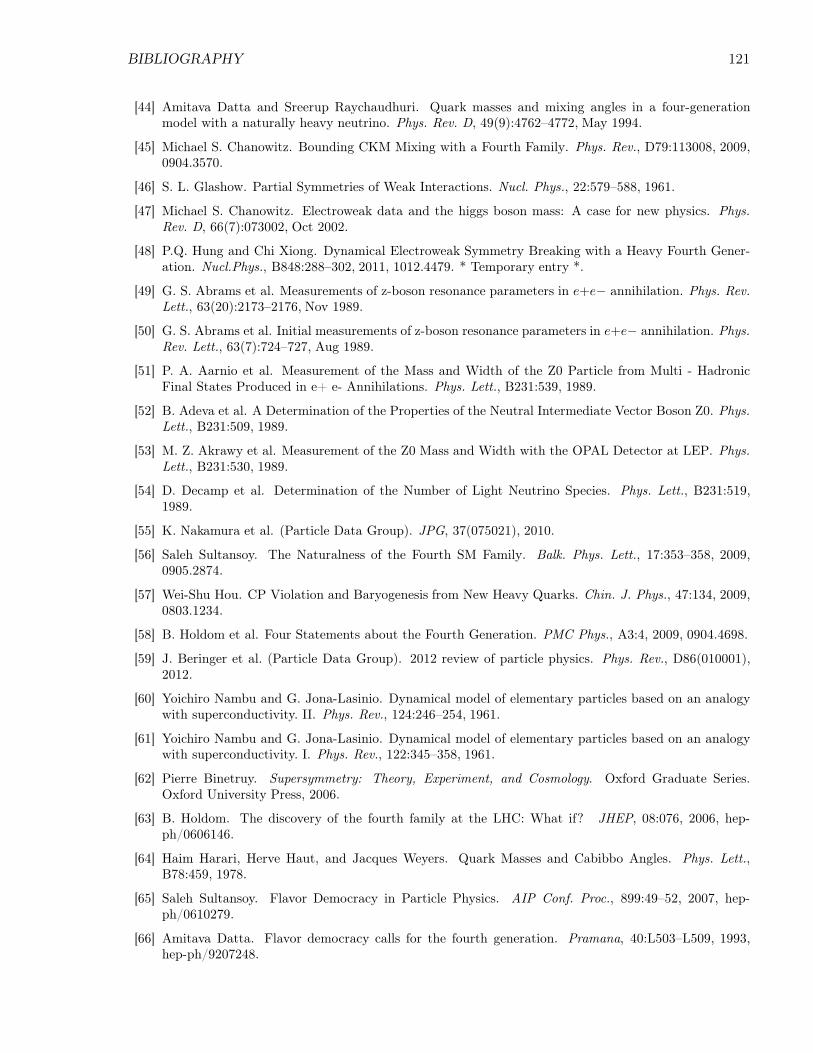
BIBLIOGRAPHY 121
[44] Amitava Datta and Sreerup Raychaudhuri. Quark masses and mixing angles in a four-generationmodel with a naturally heavy neutrino. Phys. Rev. D, 49(9):4762–4772, May 1994.
[45] Michael S. Chanowitz. Bounding CKM Mixing with a Fourth Family. Phys. Rev., D79:113008, 2009,0904.3570.
[46] S. L. Glashow. Partial Symmetries of Weak Interactions. Nucl. Phys., 22:579–588, 1961.
[47] Michael S. Chanowitz. Electroweak data and the higgs boson mass: A case for new physics. Phys.
Rev. D, 66(7):073002, Oct 2002.
[48] P.Q. Hung and Chi Xiong. Dynamical Electroweak Symmetry Breaking with a Heavy Fourth Gener-ation. Nucl.Phys., B848:288–302, 2011, 1012.4479. * Temporary entry *.
[49] G. S. Abrams et al. Measurements of z-boson resonance parameters in e+e− annihilation. Phys. Rev.
Lett., 63(20):2173–2176, Nov 1989.
[50] G. S. Abrams et al. Initial measurements of z-boson resonance parameters in e+e− annihilation. Phys.
Rev. Lett., 63(7):724–727, Aug 1989.
[51] P. A. Aarnio et al. Measurement of the Mass and Width of the Z0 Particle from Multi - HadronicFinal States Produced in e+ e- Annihilations. Phys. Lett., B231:539, 1989.
[52] B. Adeva et al. A Determination of the Properties of the Neutral Intermediate Vector Boson Z0. Phys.
Lett., B231:509, 1989.
[53] M. Z. Akrawy et al. Measurement of the Z0 Mass and Width with the OPAL Detector at LEP. Phys.
Lett., B231:530, 1989.
[54] D. Decamp et al. Determination of the Number of Light Neutrino Species. Phys. Lett., B231:519,1989.
[55] K. Nakamura et al. (Particle Data Group). JPG, 37(075021), 2010.
[56] Saleh Sultansoy. The Naturalness of the Fourth SM Family. Balk. Phys. Lett., 17:353–358, 2009,0905.2874.
[57] Wei-Shu Hou. CP Violation and Baryogenesis from New Heavy Quarks. Chin. J. Phys., 47:134, 2009,0803.1234.
[58] B. Holdom et al. Four Statements about the Fourth Generation. PMC Phys., A3:4, 2009, 0904.4698.
[59] J. Beringer et al. (Particle Data Group). 2012 review of particle physics. Phys. Rev., D86(010001),2012.
[60] Yoichiro Nambu and G. Jona-Lasinio. Dynamical model of elementary particles based on an analogywith superconductivity. II. Phys. Rev., 124:246–254, 1961.
[61] Yoichiro Nambu and G. Jona-Lasinio. Dynamical model of elementary particles based on an analogywith superconductivity. I. Phys. Rev., 122:345–358, 1961.
[62] Pierre Binetruy. Supersymmetry: Theory, Experiment, and Cosmology. Oxford Graduate Series.Oxford University Press, 2006.
[63] B. Holdom. The discovery of the fourth family at the LHC: What if? JHEP, 08:076, 2006, hep-ph/0606146.
[64] Haim Harari, Herve Haut, and Jacques Weyers. Quark Masses and Cabibbo Angles. Phys. Lett.,B78:459, 1978.
[65] Saleh Sultansoy. Flavor Democracy in Particle Physics. AIP Conf. Proc., 899:49–52, 2007, hep-ph/0610279.
[66] Amitava Datta. Flavor democracy calls for the fourth generation. Pramana, 40:L503–L509, 1993,hep-ph/9207248.

122 BIBLIOGRAPHY
[67] S. Atag et al. Fourth SM family, breaking of mass democracy, and the CKM mixings. Phys. Rev. D,54(9):5745–5749, Nov 1996.
[68] A. K. Ciftci, R. Ciftci, and S. Sultansoy. Fourth standard model family neutrino at future linearcolliders. Phys. Rev. D, 72(5):053006, Sep 2005.
[69] Michael S. Chanowitz. Z → bb Decay Asymmetry: Lose-Lose for the Standard Model. Phys. Rev.
Lett., 87(23):231802, Nov 2001.
[70] Enrico Lunghi and Amarjit Soni. Footprints of the Beyond in flavor physics: Possible role of the TopTwo Higgs Doublet Model. JHEP, 09:053, 2007, 0707.0212.
[71] Enrico Lunghi and Amarjit Soni. Possible Indications of New Physics in B(d)-mixing and in sin(2beta) Determinations. Phys. Lett., B666:162–165, 2008, 0803.4340.
[72] Amarjit Soni, Ashutosh Kumar Alok, Anjan Giri, Rukmani Mohanta, and Soumitra Nandi. TheFourth family: A Natural explanation for the observed pattern of anomalies in B− CP asymmetries.Phys.Lett., B683:302–305, 2010, 0807.1971.
[73] D. Asner et al. Averages of b-hadron, c-hadron, and tau-lepton Properties. 2010, 1010.1589.
[74] J. Charles et al. CP violation and the CKM matrix: Assessing the impact of the asymmetric Bfactories. Eur.Phys.J., C41:1–131, 2005, hep-ph/0406184.
[75] Heavy flavor averaging group (HFAG): http://www.slac.stanford.edu/xorg/hfag/.
[76] M. Bona et al. First Evidence of New Physics in b <—> s Transitions. PMC Phys., A3:6, 2009,0803.0659.
[77] Alexander Lenz and Ulrich Nierste. Theoretical update of B(s - anti-B(s) mixing. JHEP, 06:072, 2007,hep-ph/0612167.
[78] T. Aaltonen et al. First Flavor-Tagged Determination of Bounds on Mixing-Induced CP Violation inB0_s→ J/ψφ Decays. Phys.Rev.Lett., 100:161802, 2008, 0712.2397.
[79] V.M. Abazov et al. Measurement of B0_s mixing parameters from the flavor-tagged decay B0_s →J/ψφ. Phys.Rev.Lett., 101:241801, 2008, 0802.2255.
[80] The four LEP experiments ALEPH, DELPHI, L3 and OPAL. LEP Electroweak Working Group,Status of May 2001.
[81] Precision electroweak measurements on the Z resonance. Phys. Rept., 427:257–454, 2006, hep-ex/0509008.
[82] The four LEP experiments ALEPH, DELPHI, L3 and OPAL. LEP Electroweak Working Group,Status of July 2010.
[83] Michael S. Chanowitz, M.A. Furman, and I. Hinchliffe. Weak Interactions of Ultraheavy Fermions. 2.Nucl.Phys., B153:402, 1979.
[84] Benjamin W. Lee, C. Quigg, and H. B. Thacker. Weak Interactions at Very High-Energies: The Roleof the Higgs Boson Mass. Phys. Rev., D16:1519, 1977.
[85] Abdelhak Djouadi. The Anatomy of electro-weak symmetry breaking. I: The Higgs boson in thestandard model. Phys.Rept., 457:1–216, 2008, hep-ph/0503172.
[86] Amol Dighe, Diptimoy Ghosh, Rohini M. Godbole, and Arun Prasath. Large mass splittings for fourthgeneration fermions allowed by LHC Higgs exclusion. Phys.Rev., D85:114035, 2012, 1204.3550.
[87] Frank Wilczek. Quantum chromodynamics (QCD): The modern theory of the strong interaction. Ann.
Rev. Nucl. Part. Sci., 32:177–209, 1982.
[88] Peter W. Higgs. Broken symmetries, massless particles and gauge fields. Phys. Lett., 12:132–133, 1964.
[89] Peter W. Higgs. Broken symmetries and the masses of gauge bosons. Phys. Rev. Lett., 13:508–509,1964.
BIBLIOGRAPHY 123
[90] F. Englert and R. Brout. Broken symmetry and the mass of gauge vector mesons. Phys. Rev. Lett.,13:321–322, 1964.
[91] D. Bailin and A. Love. Introduction to quantum field theory. Graduate student series in physics.Institute of physics publishing Bristol and Philadelphia, revised edition, 1986.
[92] L.D. Faddeev and V.N. Popov. Feynman Diagrams for the Yang-Mills Field. Phys.Lett., B25:29–30,1967.
[93] Vincent Rivasseau. Lecture notes - advanced quantum field theory. Ecole Normale Supérieure, Paris75005, France, 2012.
[94] Vincent Rivasesau. From perturbative to constructive renormalization. Princeton Series in Physics,2nd edition, May 1991.
[95] F.J. Dyson. Divergence of perturbation theory in quantum electrodynamics. Phys.Rev., 85:631–632,1952.
[96] Michael E. Peskin and Daniel V. Schroeder. An introduction to quantum field theory. Westview PressAdvanced book program, 1995.
[97] Emmy Noether. Invariant Variation Problems. Gott. Nachr., 1918:235–257, 1918, physics/0503066.
[98] S. L. Glashow. . PhD thesis, Harvard University, 1958. Ph.D. thesis.
[99] Chen-Ning Yang and Robert L. Mills. Conservation of Isotopic Spin and Isotopic Gauge Invariance.Phys.Rev., 96:191–195, 1954.
[100] Georges Aad et al. Observation of a new particle in the search for the Standard Model Higgs bosonwith the ATLAS detector at the LHC. 2012, 1207.7214.
[101] Serguei Chatrchyan et al. Observation of a new boson at a mass of 125 GeV with the CMS experimentat the LHC. Phys.Lett.B, 2012, 1207.7235.
[102] Ta-Pei Cheng and Ling-Fong Li. Gauge theory of elementary particle physics. Oxford Science Publi-cations. Oxford University Press, 1984.
[103] Philip W. Anderson. Plasmons, gauge invariance, and mass. Phys. Rev., 130:439–442, 1963.
[104] P. W. Anderson. Random-phase approximation in the theory of superconductivity. Phys. Rev.,112:1900–1916, 1958.
[105] Peter W. Higgs. Spontaneous Symmetry Breakdown without Massless Bosons. Phys. Rev., 145:1156–1163, 1966.
[106] Makoto Kobayashi and Toshihide Maskawa. CP Violation in the Renormalizable Theory of WeakInteraction. Prog. Theor. Phys., 49:652–657, 1973.
[107] Frederick J. Gilman and Yosef Nir. Quark mixing: The ckm picture. Ann. Rev. Nucl. Part. Sci.,40:213–238, 1990.
[108] M. L. Mehta. Random matrices and the statistical theory of energy levels. Academic Press, 1967.
[109] Howard Georgi. Lie algebras in particle physics. Westview Press Advanced book program, 1999.
[110] M. Battaglia et al. The CKM matrix and the unitarity triangle. Workshop, CERN, Geneva, Switzer-land, 13-16 Feb 2002: Proceedings. 2003, hep-ph/0304132.
[111] Markus Bobrowski, Alexander Lenz, Johann Riedl, and Jurgen Rohrwild. How much space is left fora new family of fermions? Phys. Rev., D79:113006, 2009, 0902.4883.
[112] J. Adam et al. New limit on the lepton-flavour violating decay mu -> e gamma. 2011, 1107.5547.
[113] B. Pontecorvo. Mesonium and antimesonium. Sov. Phys. JETP, 6:429, 1957.
[114] B. Pontecorvo. Neutrino experiments and the question of leptonic-charge conservation. Sov. Phys.
JETP, 26:984–988, 1968.
124 BIBLIOGRAPHY
[115] Y. Katayama, K. Matumoto, S. Tanaka, and E. Yamada. Possible unified models of elementaryparticles with two neutrinos. Prog. Theor. Phys., 28:675, 1962.
[116] Ziro Maki, Masami Nakagawa, and Shoichi Sakata. Remarks on the unified model of elementaryparticles. Prog. Theor. Phys., 28:870–880, 1962.
[117] M. C. Gonzalez-Garcia. Global analysis of neutrino data. Phys. Scripta, T121:72–77, 2005, hep-ph/0410030.
[118] Y. Suzuki. Super-Kamiokande: Present and future. Nucl. Phys. Proc. Suppl., 137:5–14, 2004.
[119] Y. Suzuki. Super-Kamiokande results on neutrino oscillations. Phys. Scripta, T121:23–28, 2005.
[120] K. Eguchi et al. First results from KamLAND: Evidence for reactor anti- neutrino disappearance.Phys. Rev. Lett., 90:021802, 2003, hep-ex/0212021.
[121] F.P. An et al. Observation of electron-antineutrino disappearance at Daya Bay. Phys.Rev.Lett.,108:171803, 2012, 1203.1669.
[122] M. H. Ahn et al. Search for electron neutrino appearance in a 250-km long- baseline experiment. Phys.
Rev. Lett., 93:051801, 2004, hep-ex/0402017.
[123] M. H. Ahn et al. Indications of Neutrino Oscillation in a 250 km Long- baseline Experiment. Phys.
Rev. Lett., 90:041801, 2003, hep-ex/0212007.
[124] A. A. Aguilar-Arevalo et al. Event Excess in the MiniBooNE Search for ν_µ → ν_e Oscillations.Phys. Rev. Lett., 105:181801, 2010, 1007.1150.
[125] Stuart Raby and Richard Slansky. Neutrino Masses - How to add them to the Standard Model. Los
Alamos Science, (25), 1997.
[126] Ettore Majorana. Theory of the Symmetry of Electrons and Positrons. Nuovo Cim., 14:171–184, 1937.
[127] Chung Wook Kim and Aihud Pevsner. Neutrinos in Physics and Astrophysics, volume 8. HarwoodAcademic Publisher, Contemporary Concepts in Physics, 1993.
[128] Ning Chen and Hong-Jian He. LHC Signatures of Two-Higgs-Doublets with Fourth Family. JHEP,1204:062, 2012, 1202.3072.
[129] Thomas Schwetz, Mariam Tortola, and J. W. F. Valle. Global neutrino data and recent reactor fluxes:status of three-flavour oscillation parameters. New J. Phys., 13:063004, 2011, 1103.0734.
[130] B. Holdom. t’ at the LHC: The physics of discovery. JHEP, 03:063, 2007, hep-ph/0702037.
[131] A. K. Ciftci, R. Ciftci, and S. Sultansoy. The fourth SM family neutrino at future linear colliders.Phys. Rev., D72:053006, 2005, hep-ph/0505120.
[132] Graham D. Kribs, Tilman Plehn, Michael Spannowsky, and Timothy M. P. Tait. Four generations andHiggs physics. Phys. Rev., D76:075016, 2007, 0706.3718.
[133] Michael S. Chanowitz, M. A. Furman, and I. Hinchliffe. Weak Interactions of Ultraheavy Fermions. 2.Nucl. Phys., B153:402, 1979.
[134] Michael S. Chanowitz, M. A. Furman, and I. Hinchliffe. Weak Interactions of Ultraheavy Fermions.Phys. Lett., B78:285, 1978.
[135] M. J. G. Veltman. Limit on Mass Differences in the Weinberg Model. Nucl. Phys., B123:89, 1977.
[136] Michael E. Peskin and Tatsu Takeuchi. A New constraint on a strongly interacting Higgs sector. Phys.
Rev. Lett., 65:964–967, 1990.
[137] Michael E. Peskin and Tatsu Takeuchi. Estimation of oblique electroweak corrections. Phys. Rev. D,46(1):381–409, Jul 1992.
[138] Johana A. Herrera, Richard H. Benavides, and William A. Ponce. Flavor changing neutral currentswith a fourth family of quarks. Phys. Rev., D78:073008, 2008, 0810.3871.
BIBLIOGRAPHY 125
[139] Michael S. Chanowitz. Higgs Mass Constraints on a Fourth Family: Upper and Lower Limits on CKMMixing. Phys. Rev., D:035018, 2010, 1007.0043.
[140] Wei-Shu Hou, Makiko Nagashima, and Andrea Soddu. Enhanced K(L) –> pi0 nu anti-nu from directCP violation in B –> K pi with four generations. Phys. Rev., D72:115007, 2005, hep-ph/0508237.
[141] Wei-Shu Hou, Makiko Nagashima, and Andrea Soddu. Large time-dependent CP violation in B/s0 sys-tem and finite D0 - anti-D0 mass difference in four generation standard model. Phys. Rev., D76:016004,2007, hep-ph/0610385.
[142] Jens Erler and Paul Langacker. Precision Constraints on Extra Fermion Generations. Phys. Rev. Lett.,105:031801, 2010, 1003.3211.
[143] Wei-Shu Hou and Chien-Yi Ma. Flavor and CP Violation with Fourth Generations Revisited. Phys.
Rev., D82:036002, 2010, 1004.2186.
[144] Ringaile Placakyte. Parton Distribution Functions. 2011, 1111.5452.
[145] Vernon Barger and Roger Phillips. Collider Physics. Addison-Wesley Publishing Company, Frontiersin Physics, 1987.
[146] X. Ruan and Z. Zhang. Impact on the Higgs Production Cross Section and Decay Branching Fractionsof Heavy Quarks and Leptons in a Fourth Generation Model. 2011, 1105.1634.
[147] T. Aaltonen et al. Combined Tevatron upper limit on gg->H->W+W- and constraints on the Higgsboson mass in fourth-generation fermion models. Phys. Rev., D82:011102, 2010, 1005.3216.
[148] T. Cuhadar-Donszelmann, Muge Karagoz, V. E. Ozcan, S. Sultansoy, and G. Unel. Fourth FamilyNeutrinos and the Higgs Boson. JHEP, 10:074, 2008, 0806.4003.
[149] V. A. Novikov, L. B. Okun, Alexandre N. Rozanov, and M. I. Vysotsky. Mass of the Higgs versusfourth generation masses. JETP Lett., 76:127–130, 2002, hep-ph/0203132.
[150] Hong-Jian He, Nir Polonsky, and Shu fang Su. Extra families, Higgs spectrum and oblique corrections.Phys. Rev., D64:053004, 2001, hep-ph/0102144.
[151] David Atwood, Sudhir Kumar Gupta, and Amarjit Soni. Detecting Fourth Generation Quarks atHadron Colliders. JHEP, 1206:105, 2012, 1104.3874.
[152] O. Cakir, A. Senol, and A. T. Tasci. Single Production of Fourth Family t′ Quarks at LHeC. Europhys.
Lett., 88:11002, 2009, 0905.4347.
[153] O. Cakir, H. Duran Yildiz, R. Mehdiyev, and I. Turk Cakir. Single Production of Fourth FamilyQuarks at the LHC. Eur. Phys. J., C56:537–543, 2008, 0801.0236.
[154] Mathieu Buchkremer, Jean-Marc Gerard, and Fabio Maltoni. Closing in on a perturbative fourthgeneration. JHEP, 1206:135, 2012, 1204.5403.
[155] M. Sahin, S. Sultansoy, and S. Turkoz. A Search for the Fourth SM Family: Tevatron still has aChance. 2010, 1009.5405.
[156] O. Cakir and V. Cetinkaya. Single Production of Fourth Family b’ Quark at the Large Hadron electronCollider. Mod. Phys. Lett., A25:2571–2577, 2010, 0912.2041.
[157] J. B. Dainton, M. Klein, P. Newman, E. Perez, and F. Willeke. Deep inelastic electron nucleonscattering at the LHC. JINST, 1:P10001, 2006, hep-ex/0603016.
[158] I. T. Cakir, H. Duran Yildiz, O. Cakir, and G. Unel. Anomalous resonant production of the fourthfamily up type quarks at the LHC. Phys. Rev., D80:095009, 2009, 0908.0123.
[159] David Cox. Search for a heavy top t′ ⇒Wq in top events. 2009, 0910.3279.
[160] Christian J. Flacco, Daniel Whiteson, and Matthew Kelly. Fourth generation quark mass limits inCKM-element space. 2011, 1101.4976.
126 BIBLIOGRAPHY
[161] Michael M.H. Luk. Searches For Fourth Generation Quarks With The CMS Detector. 2011, 1110.3246.
[162] Serguei Chatrchyan et al. Search for heavy, top-like quark pair production in the dilepton final statein pp collisions at
√s = 7 TeV. 2012, 1203.5410.
[163] T. Aaltonen et al. Search for New Particles Leading to Z+jets Final States in p anti-p Collisions ats**(1/2) = 1.96-TeV. Phys. Rev., D76:072006, 2007, 0706.3264.
[164] Georges Aad et al. Search for down-type fourth generation quarks with the ATLAS detector in eventswith one lepton and hadronically decaying W bosons. Phys.Rev.Lett., 109:032001, 2012, 1202.6540.
[165] Serguei Chatrchyan et al. Search for heavy bottom-like quarks in 4.9 inverse femtobarns of pp collisionsat sqrt(s) = 7 TeV. JHEP, 1205:123, 2012, 1204.1088.
[166] P. Achard et al. Search for heavy neutral and charged leptons in e+ e- annihilation at LEP. Phys.
Lett., B517:75–85, 2001, hep-ex/0107015.
[167] S. Sultansoy and G. Unel. ’ Silver ’ mode for the heavy Higgs search in the presence of a fourth SMfamily. 2007, 0707.3266.
[168] R. Ciftci, A. K. Ciftci, E. Recepoglu, and S. Sultansoy. Fourth SM family manifestations at CLIC.Turk. J. Phys., 27:179–186, 2003, hep-ph/0203083.
[169] Linda M. Carpenter and Arvind Rajaraman. Revisiting Constraints on Fourth Generation NeutrinoMasses. Phys. Rev., D82:114019, 2010, 1005.0628.
[170] O. Cakir and S. Sultansoy. The fourth SM family enhancement to the golden mode at the upgradedTevatron. Phys. Rev., D65:013009, 2002, hep-ph/0106312.
[171] Doug Benjamin et al. Combined CDF and D0 upper limits on gg->H W+W- and constraints on theHiggs boson mass in fourth-generation fermion models with up to 8.2 fb-1 of data. 2011, 1108.3331.
[172] M. Baak et al. Updated Status of the Global Electroweak Fit and Constraints on New Physics. 2011,1107.0975.
[173] N. Becerici Schmidt, S.A. Cetin, S. Istin, and S. Sultansoy. The Fourth Standart Model Family and theCompetition in Standart Model Higgs Boson Search at Tevatron and LHC. Eur.Phys.J., C66:119–126,2010, 0908.2653.
[174] Georges Aad et al. Limits on the production of the Standard Model Higgs Boson in pp collisions atsqrt(s) =7 TeV with the ATLAS detector. 2011, 1106.2748. * Temporary entry *.
[175] A. Nisati. Higgs searches in ATLAS. Talk given at the XXV International Symposium on Lepton
Photon Interactions at High Energies, Mumbai, India, 2011.
[176] Andrey Korytov. Combined results on SM Higgs Search with the CMS Detector. talk given at EPS
2011, Grenoble, July 2011.
[177] S. A. Cetin, T. Cuhadar-Donszelmann, M. Sahin, S. Sultansoy, and G. Unel. Impact of the relativelylight fourth family neutrino on the Higgs boson search. 2011, 1108.4071.
[178] Juste, A. for the ATLAS, CDF, CMS and D0 collaborations. Searches for the Higgs boson. Plenary
talk at DPF, Brown University, Providence, 2011.
[179] CMS Collaboration and ATLAS Collaboration. Cern experiments observe particle consistent withlong-sought higgs boson. CERN Press Release PR17.12 04.07.2012.
[180] Updated Combination of CDF and D0 Searches for Standard Model Higgs Boson Production with upto 10.0 fb−1 of Data. 2012, 1207.0449.
[181] Eric Kuflik, Yosef Nir, and Tomer Volansky. Implications of Higgs Searches on the Four GenerationStandard Model. 2012, 1204.1975.
[182] Abdelhak Djouadi and Alexander Lenz. Sealing the fate of a fourth generation of fermions. 2012,1204.1252.
BIBLIOGRAPHY 127
[183] Otto Eberhardt, Alexander Lenz, Andreas Menzel, Ulrich Nierste, and Martin Wiebusch. Status ofthe fourth fermion generation before ICHEP2012: Higgs data and electroweak precision observables.2012, 1207.0438.
[184] Otto Eberhardt, Geoffrey Herbert, Heiko Lacker, Alexander Lenz, Andreas Menzel, et al. Impact ofa Higgs boson at a mass of 126 GeV on the standard model with three and four fermion generations.2012, 1209.1101.
[185] G.C. Branco, P.M. Ferreira, L. Lavoura, M.N. Rebelo, Marc Sher, et al. Theory and phenomenologyof two-Higgs-doublet models. Phys.Rept., 516:1–102, 2012, 1106.0034.
[186] Leo Bellantoni, Jens Erler, Jonathan J. Heckman, and Enrique Ramirez-Homs. Masses of a FourthGeneration with Two Higgs Doublets. 2012, 1205.5580.
[187] Michael Geller, Shaouly Bar-Shalom, and Gad Eilam. The Need for New Search Strategies for FourthGeneration Quarks at the LHC. 2012, 1205.0575.
[188] Shaouly Bar-Shalom, Soumitra Nandi, and Amarjit Soni. Two Higgs doublets with 4th generationfermions - models for TeV-scale compositeness. Phys.Rev., D84:053009, 2011, 1105.6095.
[189] Konstantin Matchev. TASI lectures on precision electroweak physics. pages 51–98, 2004, hep-ph/0402031.
[190] F. Mandl and G. Shaw. Quantum field theory. John Wiley & Sons, The Atrium, Southern Gate,Chrichester, West Sussex PO 19 8SQ, England, revised edition edition, 2005.
[191] E. Leader and E. Predazzi. An introduction to gauge theories and modern particle physics, volume 1of Cambridge monographs on particle physics, nuclear physics and cosmology 3. Cambridge UniversityPress, 1996.
[192] J. Goldstone. Field Theories with Superconductor Solutions. Nuovo Cim., 19:154–164, 1961.
[193] Jeffrey Goldstone, Abdus Salam, and Steven Weinberg. Broken Symmetries. Phys. Rev., 127:965–970,1962.
[194] Pierre Binetruy. Lecture notes - Théories de jauge des intéractions éléctrofaibles. Lectures given atthe Ecole normale supérieure (Paris 75005, France), academic year 2011-2012.
[195] J. J. Sakurai. Modern Quantum Mechanics. Addison-Wesley Publishing Company, revised edition,1994.
[196] ALEPH Collaboration et al. Precision Electroweak Measurements and Constraints on the StandardModel. 2010, 1012.2367.
[197] M. E. Peskin, B W. Lynn, and R. G. Stuart. in Physics at LEP, LEP Jamboree, CERN Report No.
CERN-96-02, 1986.
[198] Dallas C. Kennedy. Renormalization of electroweak gauge interactions. Invited lectures given at 1991Theoretical Advanced Studies Inst., Boulder, CO, Jun 2-28, 1991.
[199] D. C. Kennedy and B. W. Lynn. Electroweak Radiative Corrections with an Effective Lagrangian:Four Fermion Processes. Nucl. Phys., B322:1, 1989.
[200] M. Kuroda, G. Moultaka, and D. Schildknecht. Direct one loop renormalization of SU(2)-L x U(1)-Yfour fermion processes and running coupling constants. Nucl. Phys., B350:25–72, 1991.